survey instruments and the reports of consumption expenditures

Motivation Main Contributions Data Identification Estimation Results Implications for empirical work Conclusions

Survey Instruments and the Reports of

Consumption Expenditures: Evidence from theConsumer Expenditure Surveys

Erich Battistin1 Mario Padula2

1University of Padova and IRVAPP

2University “Ca’ Foscari” of Venice and CSEF

University of CassinoMay 12 2011

Battistin and Padula: Padova and Ca’ Foscari

Survey Instruments and the Reports of Consumption Expenditures: Evidence from the Consumer Expenditure Surveys


Roadmap

The fundamental problem of measuring spending and CEXdata.

Conditions to point-identify the distribution of the effects ofsurvey instruments on the reporting of expenditures.

Some evidence on these effects.

Guidelines for empirical research using CEX data.




Motivation

In many countries expenditures are collected either by diariesor by retrospective questions.

Diaries improve the reporting of smaller, less salientpurchases, whereas recall interviews yield better data on lessfrequent and more salient purchases.

Neither diary nor recall data alone can provide a reliablemeasure of total expenditure.




Why the Consumer Expenditure Surveys (CEX)?

Two separate components with independent samples: theDiary Survey (DS) and the Interview Survey (IS).

Almost unique example of a large scale surrvey with thischaracteristic.

The IS and the DS overlap for nearly all categories ofconsumption for which information is collected using differentmethodologies (recall questions and diaries, respectively).

Surveys explicitly designed by the BLS to measure differenttypes of expenditure: neither survey is expected to representall aspects of consumption.




Why should we bother?

20

25

30

35

80

85

90

95

10

0

1982 1984 1986 1988 1990 1992 1994 1996 1998 2000 2002 2004

Median Median absolute deviation

Survey change: 1988

Food at grocery from the Diary SurveyEffects of survey changes

22

24

26

28

30

75

80

85

90

95

1982 1984 1986 1988 1990 1992 1994 1996 1998 2000 2002 2004

Median Median absolute deviation

Survey change: 1988

Food at grocery from the Interview SurveyEffects of survey changes

The recall question on food changed in 1988 (from usual monthlyto usual weakly spending). The reporting of expenditures is thusvery sensitive to the characteristics of the survey instrumentexploited.




Why should we bother?.5

.6.7

.8.9

1982 1984 1986 1988 1990 1992 1994 1996 1998 2000 2002 2004

Diary Survey Interview Survey

Weighted figures to account for compositional differences between samples

seasonally adjusted quarterly observationsStandard deviation of logs

Opposite policy conclusions depending on the survey instrument considered

(see Attanasio, Battistin and Ichimura, 2007, and Attanasio, Battistin, Padula,

2010).




Why should we bother?

Coefficient of variationWages Family Earnings




Main Contributions

The DS and IS samples are independent, but we provideconditions to combine them to get superior micro-data onhousehold spending using the most reliable survey modeaccording to BLS (and international) standards across allexpenditure categories.Identification of any functional of the improved measure oftotal spending (i.e. not just its mean).Characterize the effects of changing the collection mode(recall questions vs diaries) on the reporting of expenditures.Make use of multiple measurements of food spending topoint identify the distribution of these effects.




What we find

For food spending the diary and interview instruments areroughly rank preserving, in the sense that the relative positionof households in the expenditure distribution is unaffected bythe collection mode.The mean effect of changing the survey instrument (fromrecall questions to diaries) is roughly stable over time butheterogeneous with respect to several householdscharacteristics (age, education and ethnicity of the head, andhousehold composition).The effect of the survey instrument has become more dispersein the population over the years for the reporting of food.




The Consumer Expenditure Surveys

The Consumer Expenditure Surveys

US Consumer Expenditure Survey (CEX), 1982-2003, run by theBureau of Labor Statistics.

IS: rotating sample, about 5,000 CU each quarter.

DS: repeated cross-section, about 5,000 CU each year.

Both samples were increased to 7,500 from 1999, the response ratesare around 80 percent.

Common sampling frame, based on the 1980 and 1990 Censuses




The definition of expenditure categories

The definition of expenditure categoriesFood and Non-Alcoholic Beverages at Home D goodsFood and Non-Alcoholic Beverages Away from Home D goodsAlcoholic Beverages (at home and away from home) D goodsNon-Durable Goods and Services D goods

Newspapers and MagazinesNon-durable Entertainment ExpensesHousekeeping Services (DS only)Personal Care (DS only)

Housing and Public Services R goodsHome Maintenance ServicesPublic UtilitiesMiscellaneous Home Services

Tobacco and Smoking Accessories R goodsClothing, Footwear and Services R goods

Clothing, FootwearServices

Heating Fuel, Light and Power R goodsTransportation (including gasoline) R goods

Fuel for TransportationTransportation Equipment Maintenance and RepairPublic TransportationVehicle Rental and Misc. Transportation Expenses




The working sample

The working sample

Family consumption is adjusted using the OECD equivalence scale.

Real expenditures are obtained using the Current Price Indexpublished by the BLS.




The working sample

Table 1: Sample selection

Sample size before selecting out Diary sample Interview sample

Households with incomplete income response 141,061 1,529,483Non-urban households 109,166 1,274,674

Household heads aged less than 25 and more than 65 98,380 1,150,827Self-employed household head 71,486 835,453

57,608 670,292




The working sample

Table 2: Summmary statistics

1982-1987 1988-1990 1991-1995 1996-2000 2001-2003

Diary Interview Diary Interview Diary Interview Diary Interview Diary InterviewAge≤ 35 0.419 0.405 0.388 0.378 0.360 0.348 0.321 0.324 0.294 0.292(35 − 45] 0.271 0.276 0.306 0.310 0.329 0.323 0.329 0.327 0.323 0.315(45 − 55] 0.176 0.183 0.188 0.197 0.202 0.215 0.238 0.240 0.257 0.260> 55 0.134 0.136 0.118 0.116 0.108 0.114 0.112 0.109 0.125 0.133Family typeH/W only 0.172 0.157 0.174 0.157 0.163 0.156 0.158 0.158 0.160 0.157H/W, oldest child 6- 0.106 0.095 0.102 0.093 0.096 0.087 0.082 0.077 0.076 0.073H/W, oldest child 6-17 0.218 0.216 0.215 0.211 0.222 0.210 0.217 0.208 0.209 0.198H/W, oldest child 18+ 0.090 0.107 0.079 0.098 0.081 0.088 0.078 0.084 0.082 0.087All other H/W 0.043 0.047 0.044 0.046 0.045 0.049 0.049 0.048 0.050 0.051Other households 0.371 0.377 0.384 0.396 0.393 0.411 0.415 0.425 0.422 0.432EthnicityWhite 0.859 0.858 0.860 0.850 0.851 0.840 0.830 0.830 0.824 0.821Black 0.104 0.103 0.101 0.110 0.106 0.117 0.113 0.118 0.122 0.120Other 0.037 0.039 0.038 0.040 0.043 0.043 0.057 0.052 0.055 0.059EducationHigh school dropout 0.153 0.156 0.126 0.136 0.108 0.120 0.103 0.109 0.099 0.105High school graduate 0.311 0.308 0.308 0.309 0.301 0.300 0.264 0.267 0.250 0.260College dropout 0.248 0.240 0.257 0.260 0.262 0.258 0.197 0.198 0.197 0.191At least college graduate 0.288 0.296 0.309 0.295 0.328 0.322 0.435 0.425 0.454 0.444




The general setup

The general setup

Let Y1 and Y0 be the potential reports using recall questions anddiaries, respectively.

The difference Y1 − Y0 thus defines the casual effect of the surveyinstrument on the reporting of expenditures.

Let D be the a dummy for the survey instrument implemented,where D = 1 for recall questions (IS) and D = 0 for diaries (DS).

Let X be a set of characteristics of the household interviewed.

Assumption 1. For all values x there is:

(Y0,Y1)⊥D|X = x ,

e(x) ≡ P[D = 1|X = x ] ∈ (0, 1),

where e(x) is the propensity score.




The general setup

Assumption 1

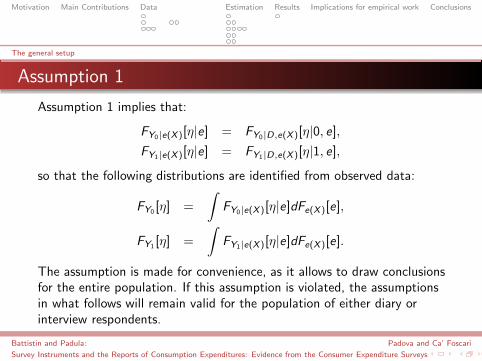
Assumption 1 implies that:

FY0|e(X )[η|e] = FY0|D,e(X )[η|0, e],

FY1|e(X )[η|e] = FY1|D,e(X )[η|1, e],

so that the following distributions are identified from observed data:

FY0 [η] =

∫FY0|e(X )[η|e]dFe(X )[e],

FY1 [η] =

∫FY1|e(X )[η|e]dFe(X )[e].

The assumption is made for convenience, as it allows to draw conclusionsfor the entire population. If this assumption is violated, the assumptionsin what follows will remain valid for the population of either diary orinterview respondents.




Food Expenditure

Food Expenditure

Three measurements of food spending available by pooling DS and ISdata:

Information on food expenditure is collected in either surveycomponent of the CEX using the same sequence of recall questionsabout usual spending over a specified period of time. This results inthe same survey instrument (i.e. recall questions) applied toindependent samples of (similar) households.

This information is then complemented in the DS by detailedrecords on food spending coming from the two weeks diary. Thisresults in different survey instruments (i.e. recall questions anddiaries) applied to the same households.




Food Expenditure

Survey Recall Question Diary

DS X XIS X




Testing assumption 1

Testing assumption 1

H0 : FY1|D,e(X )[η|0, e] = FY1|D,e(X )[η|1, e]

The null implies exchangeability of observed expenditure w.r.t. D

Random permutation to compute

p ≡ PrH0{|T∗| ≥ |Tobs |},

Bootstrap: to produce

1

100

100∑j=1

pj ,




Rank invariance

Rank invariance

Amounts to assuming that households who are highly ranked when theyfill diaries are equally ranked if they are interviewed using recall questions.

60th percentile

0.2

.4.6

.81

7 7.5 8 8.5 9

IS data DS data

Cumulative expenditure distributions by survey instrument




Slippages from rank invariance

Figure 1: Slippages from rank invariance, Years 1982-1987

0.5

11.

5de

nsity

−1 −.5 0 .5 1slippages

Distribution of slippages from rank invariance

01

23

01

23

01

23

−1 −.5 0 .5 1 −1 −.5 0 .5 1

−1 −.5 0 .5 1 −1 −.5 0 .5 1

1st decile 2nd decile 3rd decile 4th decile

5th decile 6th decile 7th decile 8th decile

9th decile 10th decile

dens

ity

slippages

raw valuesDistribution of slippages by values of true ranks





Figure 2: Slippages from rank invariance, Years 2001-2003

0.5

11.

5de

nsity

−1 −.5 0 .5 1slippages

Distribution of slippages from rank invariance

01

23

01

23

01

23

−1 −.5 0 .5 1 −1 −.5 0 .5 1

−1 −.5 0 .5 1 −1 −.5 0 .5 1

1st decile 2nd decile 3rd decile 4th decile

5th decile 6th decile 7th decile 8th decile

9th decile 10th decile

dens

ity

slippages

raw valuesDistribution of slippages by values of true ranks





Random slippages from rank invariance

Assumption 2. For all values of e(x) define: U1 = U0 + V whereV is a random variable that describes slippages whose distribution issuch that:

FV |U0,D,e(X )[η|u0, 0, e] = FV |U0,e(X )[η|u0, e]





Figure 3: The estimated distribution of slippages conditional U0

Years 1982-1987 Years 2001-2003

01

23

01

23

−1 −.5 0 .5 1 −1 −.5 0 .5 1

u0=0 u0=0.4

u0=0.6 u0=1

beta family of distributionsDistribution of slippages by values of true ranks

01

23

01

23

−1 −.5 0 .5 1 −1 −.5 0 .5 1

u0=0 u0=0.4

u0=0.6 u0=1

beta family of distributionsDistribution of slippages by values of true ranks




The distribution of slippages is the same across expenditure groups

Using the distribution of slippages

Assumption 3. For all values of e(x) and u0 the conditional distributionFV |U0,e(X )[η|u0, e] is the same across expenditure groups.




The distribution of slippages is the same across expenditure groups

Testing Assumption 3

VD=UD1 − UD

0

VR=UR1 − UR

0

H0 : FVD |e(X ),UD

0[η|e, uD0 ] = FVR|e(X ),UR

0[η|e, uR0 ]




Estimating the distribution of the survey effects

and on other expenditure categories

FV |U0,D,e(X )[η|u0, 0, e]

50 random draws from the fitted distribution of slippages and used therelationships:

U0 = FY |D,e(X )[Y0|0, e], Y1j = F−1Y |D,e(X )[U0 + Vj |1, e], j = 1, . . . , 50

to impute recall measurements Y1j onto the DS sample, and therelationships:

U1 = FY |D,e(X )[Y1|1, e], Y0j = F−1Y |D,e(X )[U1 − Vj |0, e], j = 1, . . . , 50

to impute diary measurements Y0j onto the IS sample.

∆j ≡ (Y1 − Y0j )D + (Y1j − Y0)(1− D), j = 1, . . . , 50

FY1−Y0 [η] ≡

∫

1

50

50∑

j=1

(

F∆j |e(X )[η|e])

dFe(X )[e].




Food

.88

.9.9

2.9

4.9

6Ite

rqua

rtile

rang

e

.05

.1.1

5.2

.25

Mea

n an

d m

edia

n

1988 1991 1994 1997 2000 2003

Mean Median75th−25th percentile




D goods

.96

.98

11.

021.

041.

06In

terq

uarti

le ra

nge

−.1

−.05

0.0

5M

ean

and

med

ian

1988 1991 1994 1997 2000 2003





R goods

1.42

1.44

1.46

1.48

1.5

Inte

rqua

rtile

rang

e

.05

.1.1

5.2

.25

.3M

ean

and

med

ian

1988 1991 1994 1997 2000 2003





Summarizing

Records collected using recall questions on Food overstate diaries ofabout 18 to 25 percentage points depending on the year considered,the 25th − 75th range steadily increases over time, pointing to achange of about 5 percentage points over the period considered.

For both D and R goods the mean and median survey effect aredecreasing. The median effect are negative for the former andpositive for the latter, the 25th − 75th range increasing for theformer, and non-monotonic for the latter.

For Food and D goods, the two instruments are leading toincreasingly dissimilar reports, for R to increasingly similar.




Food at home: heterogeneity in the effect of the surveyinstrument

1988-1990 1991-1995 1996-2000 2001-2003

Age≤ 35 0.218 0.191 0.249 0.238

(0.030)*** (0.025)*** (0.025)*** (0.031)***(35 − 45] 0.099 0.089 0.127 0.141

(0.031)** (0.025)*** (0.025)*** (0.031)***(45 − 55] 0.063 0.044 0.049 0.011

(0.032)* (0.026) (0.025) (0.031)EthnicityBlack 0.117 0.134 0.115 0.212

(0.029)*** (0.023)*** (0.022)*** (0.028)***Other -0.007 -0.060 0.010 -0.020

(0.044) (0.034) (0.030) (0.038)Poor 0.126 0.094 0.116 0.086

(0.024)*** (0.020)*** (0.020)*** (0.024)***Y1 0.581 0.596 0.610 0.590

(0.017)*** (0.014)*** (0.014)*** (0.017)***




D goods: heterogeneity in the effect of the surveyinstrument

1988-1990 1991-1995 1996-2000 2001-2003

Age< 35 0.008 0.011 0.013 0.013

(0.011) (0.009) (0.008) (0.011)(35, 45] -0.001 0.002 0.000 0.003

(0.011) (0.010) (0.008) (0.010)(45, 55] -0.002 -0.002 -0.003 -0.004

(0.011) (0.010) (0.008) (0.010)EthnicityBlack 0.037 0.052 0.061 0.051

(0.011)*** (0.009)*** (0.008)*** (0.010)***Other 0.014 0.016 0.027 0.010

(0.016) (0.014) (0.011)** (0.013)Poor 0.044 0.044 0.037 0.031

(0.010)*** (0.007)*** (0.007)*** (0.009)***Y1 0.647 0.629 0.619 0.626

(0.011)*** (0.012)*** (0.011)*** (0.011)***




R goods: heterogeneity in the effect of the surveyinstrument

1988-1990 1991-1995 1996-2000 2001-2003

Age< 35 0.019 0.036 0.054 0.054

(0.029) (0.025) (0.025)* (0.025)*(35, 45] 0.005 0.012 0.038 0.038

(0.028) (0.025) (0.023)* (0.025)(45, 55] -0.011 -0.008 0.003 0.002

(0.031) (0.026) (0.024) (0.026)EthnicityBlack 0.031 0.030 0.032 0.005

(0.028) (0.024) (0.018)* (0.027)Other 0.055 0.045 0.065 0.001

(0.047) (0.039) (0.029)* (0.036)Poor 0.084 0.093 0.102 0.103

(0.027)** (0.023)*** (0.021)*** (0.028)***Y1 0.478 0.460 0.518 0.513

(0.023)*** (0.022)*** (0.020)*** (0.022)***




Additional results

Additional results

For Food and D goods the probability of diaries understating recallincreases with income.

This is more so in recent years.




Interquartile range

.7.8

.91

1.1

.7.7

5.8

.85

1980 1985 1990 1995 2000 2005Year

Combined ISDS




Median absolute deviation from the median

.35

.4.4

5.5

.55

.34

.36

.38

.4.4

2

1980 1985 1990 1995 2000 2005Year

Combined ISDS




Conclusions

The collection mode for expenditure data significantly exacerbatesthe relative importance of survey errors.

The effects are sizeable, and imply that data drawn from recall anddiaries are not perfect substitute.

Reports form diary and recall need to be integrated, not only toprovides totals and means, but also to compute other moments ofthe consumption distribution.

Integrating diary and recall measures to produce micro-data on totalconsumption is made possible by exploiting an assumption of rankinvariance.




Interview Survey

Before 1988:

(1a) Since the 1st of (month, 3 months ago), what has been yourusual monthly expense at the grocery store or supermarket?

(1b) About how much of this amount was for non food items, suchas paper products, detergents, home cleaning supplies, petfoods and alcoholic beverages?

After 1988: usual monthly is replaced with usual weekly




Diary Survey

Before 1988:(1a) Since the 1st of (month, 3 months ago), have you and other members of your CU shopped at the

grocery store? (Monthly, Weekly, Never) followed by: How many times per (week, month) did youshop at the grocery store?

(1b) What was the usual amount of your purchase per visit?(1c) About how much of this amount was for food and nonalcoholic beverages?(1d) About how much of this amount was for non food items, such as paper products, detergents,

home cleaning supplies, pet foods and alcoholic beverages?

After 1988:(1a,now 3a) Since the 1st of (month, 3 months ago), what was your usual weekly expense at the grocery store

or supermarket?(1b,now 3b) About how much of this amount was for non food items, such as paper products, detergents,

home cleaning supplies, pet foods and alcoholic beverages?(1c,now 3c) Have you (or any members of your CU) purchased any food or nonalcoholic beverages from places

other than grocery stores, such as home delivery, specialty stores, bakeries, convenience stores,dairy stores, vegetable stands, or farmers markets?

(1d) What was your usual weekly expense at these places?




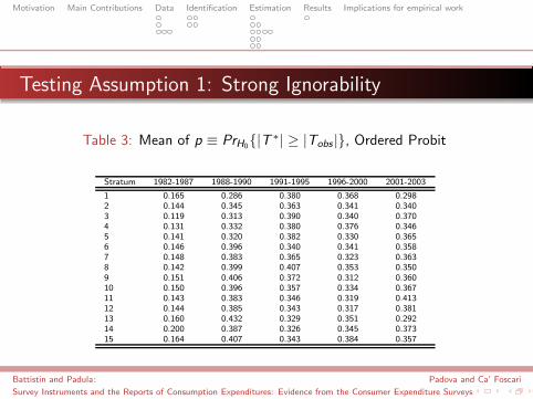
Testing Assumption 1: Strong Ignorability

Table 3: Mean of p ≡ PrH0{|T∗| ≥ |Tobs |}, Ordered Probit

Stratum 1982-1987 1988-1990 1991-1995 1996-2000 2001-2003

1 0.165 0.286 0.380 0.368 0.2982 0.144 0.345 0.363 0.341 0.3403 0.119 0.313 0.390 0.340 0.3704 0.131 0.332 0.380 0.376 0.3465 0.141 0.320 0.382 0.330 0.3656 0.146 0.396 0.340 0.341 0.3587 0.148 0.383 0.365 0.323 0.3638 0.142 0.399 0.407 0.353 0.3509 0.151 0.406 0.372 0.312 0.36010 0.150 0.396 0.357 0.334 0.36711 0.143 0.383 0.346 0.319 0.41312 0.144 0.385 0.343 0.317 0.38113 0.160 0.432 0.329 0.351 0.29214 0.200 0.387 0.326 0.345 0.37315 0.164 0.407 0.343 0.384 0.357




Testing Assumption 1: Strong Ignorability

Table 4: Mean of p ≡ PrH0{|T∗| ≥ |Tobs |}, Mann-Whitney

Stratum 1982-1987 1988-1990 1991-1995 1996-2000 2001-2003

1 0.144 0.267 0.370 0.358 0.2842 0.115 0.331 0.376 0.334 0.3143 0.095 0.323 0.400 0.337 0.3524 0.105 0.337 0.385 0.374 0.3585 0.117 0.318 0.379 0.330 0.3656 0.125 0.392 0.351 0.347 0.3457 0.121 0.392 0.374 0.324 0.3488 0.123 0.412 0.399 0.347 0.3679 0.135 0.428 0.397 0.311 0.37110 0.133 0.401 0.363 0.336 0.37111 0.125 0.380 0.335 0.314 0.41412 0.127 0.386 0.349 0.326 0.39413 0.149 0.441 0.319 0.351 0.27614 0.196 0.374 0.331 0.344 0.35115 0.150 0.411 0.368 0.396 0.350




Testing Assumption 3: Common distribution for slippages

Table 5: Mean of p ≡ PrH0{|T∗| ≥ |Tobs |}, Ordered Probit

Stratum 1982-1987 1988-1990 1991-1995 1996-2000 2001-2003

1 0.451 0.469 0.489 0.494 0.4762 0.475 0.501 0.479 0.490 0.4783 0.477 0.477 0.510 0.512 0.5174 0.452 0.509 0.501 0.487 0.4805 0.464 0.525 0.498 0.462 0.4806 0.452 0.488 0.499 0.491 0.5567 0.466 0.476 0.493 0.502 0.5138 0.451 0.490 0.488 0.493 0.4989 0.430 0.491 0.502 0.519 0.47610 0.466 0.502 0.498 0.491 0.51311 0.461 0.493 0.501 0.483 0.48812 0.452 0.504 0.497 0.512 0.48813 0.462 0.472 0.495 0.510 0.48614 0.427 0.535 0.495 0.487 0.48615 0.430 0.511 0.519 0.515 0.443




Testing Assumption 3: Common distribution for slippages

Table 6: Mean of p ≡ PrH0{|T∗| ≥ |Tobs |}, Mann-Whitney

Stratum 1982-1987 1988-1990 1991-1995 1996-2000 2001-2003

1 0.463 0.441 0.479 0.486 0.4612 0.481 0.503 0.466 0.488 0.4743 0.513 0.468 0.501 0.499 0.4914 0.471 0.517 0.500 0.507 0.4775 0.474 0.515 0.497 0.454 0.4646 0.494 0.491 0.471 0.491 0.5207 0.485 0.462 0.480 0.502 0.5018 0.463 0.484 0.468 0.473 0.4969 0.449 0.484 0.492 0.523 0.47110 0.466 0.493 0.501 0.488 0.50611 0.488 0.490 0.478 0.461 0.48412 0.468 0.488 0.491 0.498 0.47713 0.476 0.464 0.488 0.490 0.46614 0.458 0.497 0.493 0.488 0.47215 0.443 0.503 0.509 0.512 0.457



survey instruments and the reports of consumption expenditures

Documents