surface topography mission (stm) sral/mwr l2 … · and gen_cor_ran_01 algorithms ......

CLS 8-10 Rue Hermès - Parc Technologique du Canal - 31520 Ramonville St-Agne - FRANCE

Telephone 05 61 39 47 00 Fax 05 61 75 10 14

SENTINEL-3 Products and Algorithms Definition (S3PAD)

Surface Topography Mission (STM) SRAL/MWR L2 Algorithms Definition, Accuracy

and Specification [SD-03] [SD-07]

Reference: CLS-DOS-NT-09-119

Nomenclature: S3PAD-RS-CLS-SD03-00017

Issue: 8 rev 0

Date: 1 June 2011

Surface Topography Mission (STM) SRAL/MWR L2 Algorithms Definition, Accuracy and Specification

[SD-03] [SD-07]

CLS-DOS-NT-09-119 Iss :8.0 - date: 01/06/11 - Nomenclature : S3PAD-RS-CLS-SD03-00017 i.2

Proprietary information: no part of this document may be reproduced divulged or used in any form without prior permission from CLS.

Chronology Issues:

Issue: Date: Reason for change:

1rev0 20/04/2009 Draft issue

2rev0 31/07/2009 Adding algorithms specifications. Part of the PDR package

3rev0 10/11/2009 Accounting for the conclusions of the PDR meeting (RIDs 56, 57, 102, 103, 104, 106, 107, 108, 109, 137, 138, 139, 147, 148, 151, 153, 156, 158, 159, 161, 164, 166, 168, 169, 170, 171, 173, 189, 203, 204)

4rev0 31/03/2010 Proposal of routines from public libraries instead of NAG in ALT_RET_OCE_01 algorithm

Specifications of innovative algorithms selected during PDR (from SD-04).

Algorithms GEN_ENV_TID_02/04/05 updated.

Updates for CDR package.

5rev0 30/06/2010 Correction of the condition for eq. 15 in ALT_MAN_TIM_01 algorithm

Ordering the algorithms based on the name convention (CDR RID#138) – all sections

Accounting for CDR RID#65 – section 2.5.6

Accounting for CDR RID#70 for CLS algorithms – sections 2.20.3.3, 2.20.4.3 and 2.46.4.3Modification of the conditions for post-classification correction (step 5) in GEN_ENV_SUR_02 algorithm

Accounting for CDR RID#68 regarding the use of librairies – section 2.32.2

Modification of the processing for GEN_ENV_DIS_01 algorithm

Accounting for CDR RID#71 – section 2.10

Accounting for CDR RID#70 for MSSL algorithms – sections 2.6, 2.10, 2.12, 2.16, 2.17, 2.18, 2.22, 2.23, 2.29, 2.31, 2.39, 2.40



Accounting for CDR RID#139 – section 1.3.1

6rev0 30/09/2010 Modification of ALT_RET_ICE_02, ALT_PHY_RAN_01


[SD-03] [SD-07]



Chronology Issues:

Issue: Date: Reason for change:

and GEN_COR_RAN_01 algorithms

Clarification of the naming of the output of GEN_COR_RAN_02 algorithm (fluctuations of the sea surface topography)

Modification of the output “Number of elementary measurements in the averaged measurement” of ALT_MAN_TIM_01 algorithm

7rev0 12/01/2011 Update for TRR0

Correction of algorithm RAD_PHY_GEN_02 (inversion in the neural network inputs) – section 2.55

Correction of algorithm ALT_MAN_TIM_01 (equations 35, 36 and 37) – section 2.13

Correction of the origin of the ECMWF model coefficients in GEN_COR_RAN_01 algorithm (section 2.35)

8rev0 01/06/2011 Update for QR

Correction of algorithm ALT_PHY_GEN_02 (condition on the latitude threshold)) – section 2.19

Correction of ALT_PHY_GEN_03 – section 2.20

People involved in this issue:

Written by (*):

JP DUMONT

F SOULAT

A VERNIER

D BROCKLEY (MSSL)

Date + Initials:( visa ou ref)

Checked by (*):

A BLUSSON


Approved by (*): L AMAROUCHE


Application authorized by (*) :

P FEMENIAS (ESA)

N. PICOT (CNES)


*In the opposite box: Last and First name of the person + company if different from CLS


[SD-03] [SD-07]



Index Sheet :

Context: /

Keywords: /

Hyperlink: /

Distribution:

Company Means of distribution Names

ESA Electronic file P. FEMENIAS, H. REBHAN, C. LODDO

CNES Electronic file N. PICOT, J. LAMBIN, F. MERCIER

CLS Notification L. AMAROUCHE, JP. DUMONT, F. SOULAT, P. SICARD, A. BLUSSON, G. DIBARBOURE, JJ. VALETTE, S. LABROUE

ACS Electronic file PL. MANTOVANI, M. ANTONACCI

UCL/MSSL Electronic file S. BAKER, D. BROCKLEY

EUMETSAT Electronic file H. WILSON

List of tables and figures

List of tables:

List of figures:

Figure 1 - Data Management and scientific core of the algorithms 2

Figure 2 - SAR ocean retracker global software structure 52

Figure 3 - Geographical masks: in blue for winter and in red for summer. 77


[SD-03] [SD-07]



List of items to be defined or to be confirmed

List of TBC:

List of TBD:

Open source for fitting method. ....................................................................... 55


[SD-03] [SD-07]



Applicable documents / reference documents

The issue and date of the AD and RD are provided in the CIDL (AD 4).

AD 1 : GMES Sentinel-2 and Sentinel-3 Products and Algorithms Definition – Statement of Work GMES-DFPR-EOPG-SW-07-0008

AD 2 : Surface Topography Mission (STM) – L0 and L1b Products Specifications [SY-04] S4-IF-CLS-SY-00061

AD 3 : Guidelines for Sentinel-3 GMES Products Definition GMESPH-DME-TEC-TNO09-E

AD 4 : Surface Topography Mission (STM) Products and Algorithms Definition Configuration Items Data List [MD-09] S3PAD-CS-CLS-MD09-00006

AD 5 : Surface Topography Mission (STM) Products and Algorithms Definition Lists of Acronyms and Abbreviations [MD-06] S3PAD-LI-CLS-MD06-00004

AD 6 : Surface Topography Mission (STM) Products and Algorithms Definition Schedules and Deliverables [MD-03] S3PAD-SC-CLS-MD03-00002

AD 7 : Surface Topography Mission (STM) – L0 and L1b SRAL Algorithms Definition, Accuracy and Specification [SY-24] S3-RS-CLS-SY-00017

AD 8 : Surface Topography Mission (STM) - L2 Mechanisms Specification [SD-07] S3PAD-RS-CLS-SD07-00024

AD 9 : Surface Topography Mission (STM) - SRAL/MWR L2 Input/Output Data Definition [SD-09] S3PAD-RS-CLS-SD09-00018

AD 10 : Surface Topography Mission (STM) – SRAL/MWR L2 Processing Chain Specification [SD-07] S3PAD-RS-CLS-SD07-00022

AD 11 : Surface Topography Mission (STM) – SRAL/MWR L2 Data Management Algorithms Specification [SD-07] S3PAD-RS-CLS-SD07-00023


[SD-03] [SD-07]



AD 12 : A Quality Assurance Framework for Earth Observation - Key Guidelines Version: 2.0 – September 2008

AD 13: Surface Topography Mission (STM) - SRAL/MWR L2 Interface Requirements Definition S3PAD-RS-CLS-SD12-00044

AD 14: Surface Topography Mission (STM) - Algorithms Nomenclature S3PAD-RS-CLS-SD03-00025

RD 1 : GMES Sentinel-3 Topography Mission Products and Algorithms Definition : Technical Proposal AO/1-5428/07/I-EC, CLS-DOS-PR-07-046

RD 2 : ENVISAT-Ice Detailed Processing Model Document, Issue 3 Rev. 6 12133/96/NL-GS-DPM

RD 3 : Definition of the RA-2 Level 2 Ocean and Ice Retracking Algorithms, Issue 1 Rev. 0 PO-NT-RAA-003-CLS

RD 4 : RA-2 Retracking Comparisons over Ocean Surfaces, Issue 3 Rev. 1 CLS.OC/NT/95.028

RD 5 : The Art of Scientific Computing in C (Edition 2). William H. Press, Brian P. Flaneery, Saul A. Teukolsky, William T. Vetterling Numerical Recipes

RD 6 : Algorithm Definition, Accuracy and Specification – Bibli_Alti : Altimeter Level 1b Processing SALP-ST-M2-EA-15596-CN

RD 7 : Algorithms Specifications (Ocean and Ice2 FDGDR Processing), Issue 3 Rev. 5 PO-SP-RAA-0006-CLS

RD 8 : Algorithm Definition, Accuracy and Specification – Bibli_Alti : Altimeter Level 2 Processing SALP-ST-M2-EA-15598-CN

RD 9 : NAG Fortran Library Manual – Mark 18 12133/96/NL-GS-DPM

RD 10 : Minutes of the CLS Sentinel-3 PAD PM6 Meeting S3PAD-MN-CLS-MD05-00050


[SD-03] [SD-07]



Contents

1. Introduction .................................................................................. 1

1.1. Aim ....................................................................................... 1

1.2. Definitions .............................................................................. 1

1.3. General rules .......................................................................... 1

1.4. Correspondence with SD documents .............................................. 2

2. Algorithms Definition and Specification ............................................... 3

2.1. ALT_COR_BAC_01 - To compute the corrected retracked backscatter coefficients ................................................................................... 3

2.2. ALT_COR_GEN_01 - To compute the modeled instrumental corrections on the retracked parameters (Ku-band) ............................................... 4

2.3. ALT_COR_GEN_02 - To compute the modeled instrumental corrections on the retracked parameters (C-band) ................................................. 6

2.4. ALT_COR_MIS_01 - To compute the corrected squared mispointing angle8

2.5. ALT_COR_RAN_01 - To compute the Doppler correction .................... 9

2.6. ALT_COR_RAN_02 - To compute the General Doppler Correction (all) . 10

2.7. ALT_COR_RAN_03 - To compute the corrected retracked altimeter ranges ....................................................................................... 12

2.8. ALT_COR_RAN_04 - To compute the sea state biases ...................... 13

2.9. ALT_COR_RAN_05 - To compute the dual-frequency ionospheric corrections ................................................................................. 14

2.10. ALT_COR_RAN_06 – To calculate the applicable set of corrections (LRM Ice; SAR Sea-Ice, Margin) ................................................................ 16

2.11. ALT_COR_SWH_01 - To compute the corrected retracked significant waveheights ................................................................................ 17

2.12. ALT_MAN_INT_01 – To perform short-arc along-track interpolation ... 18

2.13. ALT_MAN_TIM_01 – To compute 1-Hz time tags ............................ 20

2.14. ALT_MAN_WAV_02 – To discriminate waveforms .......................... 22

2.15. ALT_PHY_BAC_01 - To compute the retracked backscatter coefficients24


[SD-03] [SD-07]



2.16. ALT_PHY_BAC_02 - To compute the backscatter coefficient (SAR, Sea-Ice, Margin) ................................................................................. 25

2.17. ALT_PHY_BAC_03 - To compute the backscatter coefficient (LRM, Ice)26

2.18. ALT_PHY_GEN_01 - To compute the elevation and location of echoing points (LRM, Ice ; SAR, Margin)......................................................... 27

2.19. ALT_PHY_GEN_02 - To compute the rain flag .............................. 28

2.20. ALT_PHY_GEN_03 - To compute the rain rate .............................. 30

2.21. ALT_PHY_RAN_01 - To compute the retracked altimeter ranges ...... 31

2.22. ALT_PHY_RAN_02 – To compute the surface height anomaly (SAR, Sea-Ice) ........................................................................................... 32

2.23. ALT_PHY_RAN_03 – To compute the freeboard ............................ 33

2.24. ALT_PHY_SNR_01 - To compute the SNR from the estimates of the amplitude and of the thermal noise level of the waveforms .................... 34

2.25. ALT_PHY_SWH_01 - To compute SWH from the retracked composite Sigma ........................................................................................ 35

2.26. ALT_PHY_WIN_01 - To correct the backscatter coefficients for atmospheric attenuation and to compute the 10 meter altimeter wind speed36

2.27. ALT_RET_ICE_01 – To perform the ice-1 (OCOG) retracking (SAR sea-ice, margin ; LRM ice) .................................................................... 37

2.28. ALT_RET_ICE_02 - To perform the ice-2 retracking (LRM) ............... 39

2.29. ALT_RET_ICE_03 – To perform the “function fit” retracking (SAR, Sea-Ice) ........................................................................................... 42

2.30. ALT_RET_ICE_04 - To merge MLE4 results into the ice chain (LRM Ice)44

2.31. ALT_RET_ICE_05 - To perform the SAR ice-margin WW retracking (SAR ice margin) ................................................................................. 45

2.32. ALT_RET_OCE_01 - To perform the ocean retracking (LRM) ............ 47

2.33. ALT_RET_OCE_02 - To perform ocean/coastal zone retracking (SAR) . 51

2.34. GEN_COR_ORB_01 - To derive the orbital altitude rate with respect to the reference MSS/geoid ................................................................ 56

2.35. GEN_COR_RAN_01 - To compute the 10 meter wind vector, the surface pressure and the mean sea surface pressure from ECMWF model, the dry and wet tropospheric “operational” corrections (ocean surfaces) and the dry and wet tropospheric “pseudo-operationnal” corrections (continental surfaces) 57

2.36. GEN_COR_RAN_02 - To compute the high frequency fluctuations of the


[SD-03] [SD-07]



sea surface topography from MOG2D model ........................................ 62

2.37. GEN_ENV_BAT_01 - To compute the ocean depth / land elevation .... 63

2.38. GEN_ENV_DIS_01 - To compute distance to shore ......................... 64

2.39. GEN_ENV_ECH_01 - To determine the echo direction (SAR, Margin) .. 65

2.40. GEN_ENV_ECH_02 - To determine the echo direction (LRM, Ice) ...... 68

2.41. GEN_ENV_GEO_01 - To compute the geoid height ......................... 70

2.42. GEN_ENV_MDT_01 - To compute the mean dynamic topography height71

2.43. GEN_ENV_MET_01 - To compute the inverted barometer effect ....... 72

2.44. GEN_ENV_MSS_01 - To compute the mean sea surface height .......... 73

2.45. GEN_ENV_SUR_01 - To determine the radiometer surface type ........ 74

2.46. GEN_ENV_SUR_02 - To compute the Ocean/Sea-Ice flag and Classes Memberships ............................................................................... 76

2.47. GEN_ENV_SUR_03 - To compute the Continental Ice flag ................ 78

2.48. GEN_ENV_TID_01 - To compute the solid earth and the equilibrium long period ocean tide heights ......................................................... 80

2.49. GEN_ENV_TID_02 - To compute the non equilibrium long period ocean tide height .................................................................................. 82

2.50. GEN_ENV_TID_03 - To compute the diurnal and semidiurnal elastic ocean tide height and the load tide height (solution 2 – 11 waves) ............ 84

2.51. GEN_ENV_TID_04 - To compute the diurnal and semidiurnal elastic ocean tide height and the load tide height (solution 1 – 28 components) ... 86

2.52. GEN_ENV_TID_05 - To compute the pole tide height ..................... 88

2.53. RAD_PHY_ATT_01 - To compute the SRAL sigma0 atmospheric attenuations ................................................................................ 90

2.54. RAD_PHY_GEN_01 - To compute the MWR geophysical parameters at SRAL time tag .............................................................................. 91

2.55. RAD_PHY_GEN_02 - To compute the wet troposphere correction at SRAL time tag (using SST and Gamma parameters) ................................ 92

2.56. RAD_PHY_GEN_03 – To compute the wet tropospheric composite correction .................................................................................. 93

2.57. RAD_PHY_TEM_01 – To co-localize the radiometer pixels ............... 95


[SD-03] [SD-07]



Annexe A - List of acronyms ............................................................... 97


[SD-03] [SD-07]

CLS-DOS-NT-09-119 Iss :8.0 - date: 01/06/11 - Nomenclature : S3PAD-RS-CLS-SD03-00017 1


1. Introduction

1.1. Aim

This document is aimed at defining and specifying the “scientific” algorithms used in the Level 2 processing of the Sentinel-3 Surface Topography Mission SRAL and MWR data, which is defined in the L2 Processing Specification document (AD 10).

These definitions and specifications has been carried out in the frame of the definition of Data Products, Level 2 Processing Algorithms and associated Data Processing Prototypes for the ESA Sentinel-3 mission, within the context of Global Monitoring for Environment and Security (GMES), awarded by ESA to a consortium composed of CLS, UCL/MSSL and ACS, led by CLS (see AD 1).

1.2. Definitions

1.2.1. General Terminology

“Scientific” algorithms represent the core of the processing. They are dissociated from “Data management” algorithms (see AD 11), ensuring functions such as data acquisition, data selection and preparation, units conversions, general checks, products generation, processing management, etc., which strongly depend on the format of the input and output data.

The Definition of the altimeter Level 2 scientific algorithms, provided in this document, consists of the identification and the description of their main functions. It will provide the reader with an overview of the procedures and a global understanding of the algorithms.

The Specifications of the altimeter Level 2 scientific algorithms, provided in this document, together with the specifications of the data management algorithms as well as the corresponding interfaces documents, are intended for the team in charge of the software development.

1.2.2. Instrument Data Levels

See AD 9 – Section 1.2.1.

1.2.3. Anciliary/Auxiliary and Dynamic/Static Data*


1.2.4. Altimeter Terminology


1.3. General rules

1.3.1. Algorithms Description

Each scientific algorithm is described, using the following items:

Name and identifier of the algorithm (see AD 14)

Heritage (mission for which the algorithm is used or derived)

Function

Algorithm Definition:


[SD-03] [SD-07]



Input data

Output data

Mathematical statement

As previously mentioned, only the scientific core of each algorithm is specified in this document. For each algorithm, the input data (1) identified in the "Algorithm definition" section corresponds to the input data required for the global processing (Data Management and Scientific Core), while the input data (2) identified in the "Algorithm specification" section corresponds to the data requested for the scientific core only.

Data ManagementData ManagementScientific coreScientific core

Algorithm

(1) (2)Data ManagementData Management

Scientific coreScientific core

Algorithm

(1) (2)

Figure 1 - Data Management and scientific core of the algorithms

The general information necessary for a global understanding of the algorithm within the overall processing is provided in the “Algorithm definition” sections.

1.3.2. Basic rules

The following basic rules are applied to the specification of the algorithms:

Elementary functions that are common to several algorithms (also called “mechanisms”) are specified in the L2 Mechanisms Specification document.

The input and output data are always identified by a precise description, an explicit name (that could be used in the coding phase), a unit and, if necessary, a reference system

Regarding the errors that may occur during the processing functions (for example, negative argument for logarithmic or square root functions), the algorithms systematically output an execution status. The building and the management of this information will be defined during the architectural design of the software.

Regarding the representation of tables, the following conventions are used in the following:

X[N1:N2] represents a one-dimension table whose elements are X(i) (or Xi) with i [N1, N2]

X[N1:N2][M1:M2] represents a two-dimension table whose elements are X(i,j) (or Xij) with i [N1,N2] and j [M1,M2]

And so on

Regarding the representation of complex signals, two conventions are used in the following:

Either distinct real and imaginary parts ("I" and "Q")

Or complex signal "IQ" corresponding to I+jQ

1.4. Correspondence with SD documents

The correspondence between this document and the SD documents is described in AD 4 and AD 5.


[SD-03] [SD-07]



2. Algorithms Definition and Specification

2.1. ALT_COR_BAC_01 - To compute the corrected retracked backscatter coefficients

2.1.1. Heritage

Jason-1, Jason-2

2.1.2. Function

To compute the corrected retracked backscatter coefficients (main and auxiliary bands).

2.1.3. Algorithm Definition

2.1.3.1. Input data

Altimeter configuration data

Backscatter coefficient:

Retracked backscatter coefficient and associated validity flag

Instrumental correction:

Backscatter modeled instrumental coefficient correction

AGC instrumental errors correction

Internal calibration correction

Processing parameters (SAD):

Backscatter coefficient system bias

2.1.3.2. Output data

Corrected retracked backscatter coefficients

Net instrumental correction

2.1.3.3. Mathematical statement

The estimates of the retracked backscatter coefficients are already corrected through the scaling factors for Sigma0 evaluation, for the AGC errors and the internal calibration (see AD 7). The two following corrections are added:

the modeled instrumental correction

the system bias

(1) 2 states: "valid" or "invalid" (2) Value to be selected according to the processed band (altimeter configuration data)


[SD-03] [SD-07]



2.2. ALT_COR_GEN_01 - To compute the modeled instrumental corrections on the retracked parameters (Ku-band)

2.2.1. Heritage

TOPEX/POSEIDON, Jason-1, Jason-2

2.2.2. Function

To compute the modeled corrections of the instrumental errors on the altimetric estimates (altimeter range, altimeter range rate, significant waveheight, backscatter coefficient and square of the mispointing angle - (main band), using correction tables depending on significant waveheight and signal to noise ratio.


2.2.3.1. Input data


Signal to noise ratio:

Signal to noise ratio and associated validity flag

Significant waveheight:

Significant waveheight and associated validity flag

Instrumental correction tables (SAD) (1):

Main band altimeter range correction table

Main band significant waveheight correction table

Main band backscatter coefficient correction table

Main band squared mispointing angle correction table


Default value for the inputs of the correction tables


Main band altimeter range modeled instrumental correction

Main band significant waveheight modeled instrumental correction

Main band backscatter modeled instrumental coefficient correction

Main band squared mispointing modeled instrumental coefficient correction


Principle

The imperfections of the altimeter components lead to errors on the altimetric estimates. To provide accurate measurements, a complete knowledge of these errors (source and quantization of their effects) is required.

(1) Including features such as lower bound, upper bound and step for each input


[SD-03] [SD-07]



The following errors are accounted for:

errors of the on-board software

errors due to the low-pass filtering

errors due to the leakage spikes

errors due to the on-board FFT

errors due to the PTR

Nevertheless, the linearity of these errors is not obvious at all, and a separate correction for each effect is probably not consistent with the instrument behavior. An integrated modeling of these errors is thus necessary.

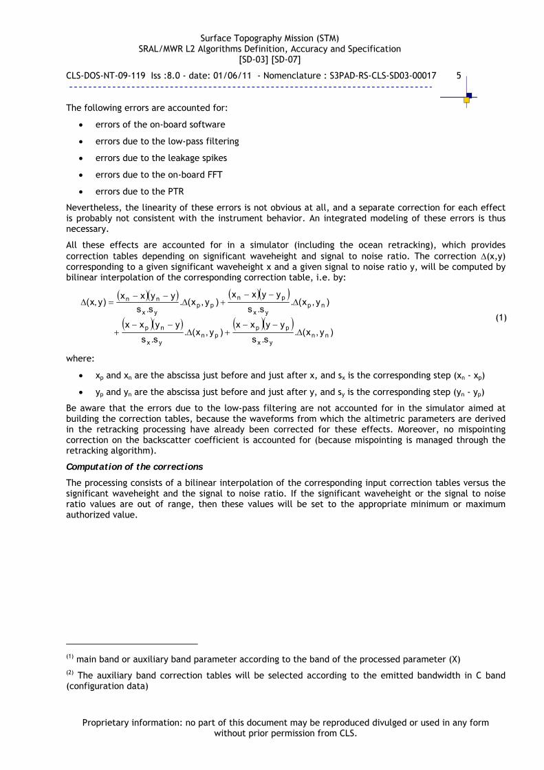
All these effects are accounted for in a simulator (including the ocean retracking), which provides correction tables depending on significant waveheight and signal to noise ratio. The correction (x,y) corresponding to a given significant waveheight x and a given signal to noise ratio y, will be computed by bilinear interpolation of the corresponding correction table, i.e. by:

)y,x(.

s.s

yyxx)y,x(.

s.s

yyxx

)y,x(.s.s

yyxx)y,x(.

s.s

yyxx)y,x(

nnyx

pppn

yx

np

npyx

pnpp

yx

nn

(1)

where:

xp and xn are the abscissa just before and just after x, and sx is the corresponding step (xn - xp)

yp and yn are the abscissa just before and just after y, and sy is the corresponding step (yn - yp)

Be aware that the errors due to the low-pass filtering are not accounted for in the simulator aimed at building the correction tables, because the waveforms from which the altimetric parameters are derived in the retracking processing have already been corrected for these effects. Moreover, no mispointing correction on the backscatter coefficient is accounted for (because mispointing is managed through the retracking algorithm).

Computation of the corrections

The processing consists of a bilinear interpolation of the corresponding input correction tables versus the significant waveheight and the signal to noise ratio. If the significant waveheight or the signal to noise ratio values are out of range, then these values will be set to the appropriate minimum or maximum authorized value.

(1) main band or auxiliary band parameter according to the band of the processed parameter (X) (2) The auxiliary band correction tables will be selected according to the emitted bandwidth in C band (configuration data)


[SD-03] [SD-07]



2.3. ALT_COR_GEN_02 - To compute the modeled instrumental corrections on the retracked parameters (C-band)

2.3.1. Heritage


2.3.2. Function

To compute the modeled corrections of the instrumental errors on the altimetric estimates (altimeter range, altimeter range rate, significant waveheight and backscatter coefficient - (auxiliary band), using correction tables depending on significant waveheight and signal to noise ratio.


2.3.3.1. Input data


Signal to noise ratio:

Signal to noise ratio and associated validity flag



Instrumental correction tables (SAD) (1):

Auxiliary band altimeter range correction tables

Auxiliary band significant waveheight correction tables

Auxiliary band backscatter coefficient correction tables


Default value for the inputs of the correction tables


Auxiliary band altimeter range modeled instrumental correction

Auxiliary band significant waveheight modeled instrumental correction

Auxiliary band backscatter modeled instrumental coefficient correction


Principle

The imperfections of the altimeter components lead to errors on the altimetric estimates. To provide accurate measurements, a complete knowledge of these errors (source and quantization of their effects) is required.

The following errors are accounted for:

errors of the on-board software

(1) Including features such as lower bound, upper bound and step for each input


[SD-03] [SD-07]



errors due to the low-pass filtering

errors due to the leakage spikes

errors due to the on-board FFT

errors due to the PTR

Nevertheless, the linearity of these errors is not obvious at all, and a separate correction for each effect is probably not consistent with the instrument behavior. An integrated modeling of these errors is thus necessary.

All these effects are accounted for in a simulator (including the ocean retracking), which provides correction tables depending on significant waveheight and signal to noise ratio. The correction (x,y) corresponding to a given significant waveheight x and a given signal to noise ratio y, will be computed by bilinear interpolation of the corresponding correction table, i.e. by:

)y,x(.

s.s

yyxx)y,x(.

s.s

yyxx

)y,x(.s.s

yyxx)y,x(.

s.s

yyxx)y,x(

nnyx

pppn

yx

np

npyx

pnpp

yx

nn

(1)

where:

xp and xn are the abscissa just before and just after x, and sx is the corresponding step (xn - xp)

yp and yn are the abscissa just before and just after y, and sy is the corresponding step (yn - yp)

Be aware that the errors due to the low-pass filtering are not accounted for in the simulator aimed at building the correction tables, because the waveforms from which the altimetric parameters are derived in the retracking processing have already been corrected for these effects. Moreover, no mispointing correction on the backscatter coefficient is accounted for (because mispointing is managed through the retracking algorithm).

Computation of the corrections

The processing consists of a bilinear interpolation of the corresponding input correction tables versus the significant waveheight and the signal to noise ratio. If the significant waveheight or the signal to noise ratio values are out of range, then these values will be set to the appropriate minimum or maximum authorized value.

(1) main band or auxiliary band parameter according to the band of the processed parameter (X) (2) The auxiliary band correction tables will be selected according to the emitted bandwidth in C band (configuration data)


[SD-03] [SD-07]



2.4. ALT_COR_MIS_01 - To compute the corrected squared mispointing angle

2.4.1. Heritage

Jason-1, Jason-2

2.4.2. Function

To compute the corrected squared mispointing angle (main band).


2.4.3.1. Input data


Squared mispointing angle:

Retracked squared mispointing angle and associated validity flag


Squared mispointing modeled instrumental correction (main band)


Squared mispointing system bias


Corrected retracked square of the mispointing angle


The modeled instrumental correction and system bias are added to the input squared mispointing angle.

(1) 2 states: "valid" or "invalid"


[SD-03] [SD-07]



2.5. ALT_COR_RAN_01 - To compute the Doppler correction

2.5.1. Heritage

Jason-1 (Poseidon-2), Jason-2, ENVISAT

2.5.2. Function

To compute the Doppler corrections on the altimeter range.


2.5.3.1. Input data

Orbit:

Orbital altitude rate


Altimeter instrumental characterization data, i.e. for each band (Ku, C):

Emitted frequency

Pulse duration

Emitted bandwidth

Sign of the slope of the transmitted chirp


Ku-band Doppler correction

C-band Doppler correction


For each band, the Doppler correction to be added to the altimeter range is computed by:

'h.B

T.f.hDoppler (1)

where:

h' is the altitude rate

f is the emitted frequency

T is the pulse duration

B is the emitted bandwidth

= 1 is the sign of the slope of the transmitted chirp

(1) Value to be selected according to the processed band


[SD-03] [SD-07]



2.6. ALT_COR_RAN_02 - To compute the General Doppler Correction (all)

2.6.1. Heritage

Envisat, Cryosat2

2.6.2. Function

This algorithm determines the generalised Doppler correction to range, due to the effects of the

spacecraft orbit and due to line of sight variations arising over sloping surfaces. This is known as

the generalised-Doppler range correction.


2.6.3.1. Input data

Slope corrected latitude:

Slope corrected longitude:

Slope corrected height: h

Orbit (DAD)

Values extracted via the CFI [CFI-S-01]; see reference for methods.

Position of the satellite in the ITER frame: P

Velocity of the satellite in the ITER frame: v

Geophysical constants

Speed of light: c

Altimeter instrumental characterization data

Wavelength: c

Chirp slope: cS


General Doppler correction: generalD


Calculate the line of sight vector from the spacecraft to the echoing point

Using the CFI supplied functions, convert the echoing point coordinates from geodetic to Cartesian ITER reference frames

Form the line of sight unit vector: l

Calculate the component of the spacecraft velocity in the line of sight vector

lv

sv

Calculate the generalised Doppler correction:


[SD-03] [SD-07]



cc

sgeneral

Scv

D


[SD-03] [SD-07]



2.7. ALT_COR_RAN_03 - To compute the corrected retracked altimeter ranges

2.7.1. Heritage

Jason-1, Jason-2

2.7.2. Function

To compute the corrected retracked altimeter ranges (main and auxiliary bands).


2.7.3.1. Input data


Altimeter range:

Retracked altimeter range and associated validity flag

Instrumental corrections:

Doppler corrections on the altimeter range (computed at L1b and L2 levels)

Modeled instrumental correction on the retracked altimeter range

USO drift correction

Internal path correction

Platform data:

Distance antenna – COG


Altimeter range system bias


Corrected retracked altimeter range



The L1b estimates of the retracked altimeter range are already corrected through the tracker range estimates, for the USO frequency drift and the internal path correction (see AD 7). The three following corrections are added:


the system bias

the distance antenna – COG

In addition for both LRM and SAR modes, the Doppler correction corresponding to the L1b processing at the measurement location is first removed from the altimeter range and the Doppler correction estimated during the L2 processing (cf.ALT_COR_RAN_01 - To compute the Doppler correction) is then applied.

(1) 2 states: "valid" or "invalid"


[SD-03] [SD-07]



2.8. ALT_COR_RAN_04 - To compute the sea state biases

2.8.1. Heritage

TOPEX/Poseidon, ERS-1, ERS-2, Jason-1, Jason-2, ENVISAT

2.8.2. Function

To compute the sea state bias in the main and in the auxiliary frequency bands. The sea state bias is the difference between the apparent sea level as "seen" by an altimeter and the actual mean sea level.


2.8.3.1. Input data


Significant waveheight (main band)

Associated validity flag

Wind speed:

Wind speed corrected for atmospheric attenuation (W)

Sea state bias table (SAD)


Sea state bias in main and in auxiliary bands


The SSB is bilinearly interpolated from a SAD table that is provided as a function of significant waveheight (main band) and of wind speed, with same values for the main and the auxiliary bands.

(2) Value to be selected according to the processed band and the emitted bandwidth (altimeter configuration data) (1) Two states : “valid”, or “invalid” (1) I = 0 for the main band, I = 1 for the auxiliary band


[SD-03] [SD-07]



2.9. ALT_COR_RAN_05 - To compute the dual-frequency ionospheric corrections

2.9.1. Heritage

Jason 1, Jason 2, ENVISAT

2.9.2. Function

To combine the altimeter ranges in the main and auxiliary frequency bands, so as to derive the main band ionospheric correction and the auxiliary band ionospheric correction. The altimeter ranges are first corrected for sea state bias before being combined.


2.9.3.1. Input data

Altimeter range:

Corrected altimeter range (main and auxiliary bands)

Associated validity flag (main and auxiliary bands)

Sea state bias:

Sea state bias correction (main and auxiliary bands)

Altimeter instrumental characterization data:

Main and auxiliary band emitted frequencies


Ionospheric correction (main and auxiliary bands)


The following formulae assume input parameters in mm.

The main band and auxiliary band sea state bias corrections are first added to the input main band and auxiliary band altimeter ranges to correct them, because these corrections may be different for the two frequencies. Let RMain and RAux be the corresponding corrected values.

The range R corrected for ionospheric delay is given for the two frequencies by the following equations:

Main_Alt_IonoRR Main (1)

uxIono_Alt_ARR Aux

where the ionospheric corrections Iono_alt_Main and Iono_alt_Aux are obtained (in mm) by using the first order expansion of the refraction index:

2Main_f

TEC.40300Main_Alt_Iono (Main band) (2)

2Aux_f

TEC.40300Aux_Alt_Iono (Auxiliary band)

where f_Main and f_Aux are the emitted frequencies (in Hz), and where TEC is the columnar total electron content of the ionosphere, expressed in electrons/m2.

Combining equations (1) and (2) leads to:


[SD-03] [SD-07]



AuxMainAux

AuxMainKu

RR.fAux_Alt_Iono

RR.fMain_Alt_Iono

(3)

with: 22

2

MainAux_fMain_f

Aux_ff

(4)

22

2

AuxAux_fMain_f

Main_ff

For LRM mode, the algorithm is run from 20-Hz Ku- and C- band altimeter estimates.

For SAR mode, it is run from 20-Hz Ku-band altimeter estimates and 20-Hz C-band filtered estimates (computed by linear regression of 1-Hz related estimates, at the Ku-band time tag).

S3PAD-RS-CLS-SD03-00017

(1) Two states : “valid”, or “invalid”


[SD-03] [SD-07]



2.10. ALT_COR_RAN_06 – To calculate the applicable set of corrections (LRM Ice; SAR Sea-Ice, Margin)

2.10.1. Heritage

Cryosat2

2.10.2. Function

A single corrections value is created by summing all of the applicable meteorological and geophysical corrections.


2.10.3.1. Input data

Corrections

GIM Ionospheric Correction (IONO)

Inverse Barometric (IB)

Ocean Tide (OT)

Loading Tide (OLT)

Solid Earth Tide (SET)

Polar Tide (PT)

Model Wet Tropospheric (WET)

Model Dry Tropospheric (DRY)

Corrections status flags

Application flags and model choices

Surface type


Corrections: C


Select an ocean tide model (GOT or FES) based on PCONF flag

Form the summed correction as

Ocean or Sea-Ice : DRY + WET + IB + IONO + OT + OLT + SET + PT

Land : DRY + WET + IONO + OLT + SET + PT Extract snow depth and sea-ice concentration from aux files with bilinear interpolation

Note that the Mog2d is not appropriate over these surfaces and the radiometer wet correction is not available.


[SD-03] [SD-07]



2.11. ALT_COR_SWH_01 - To compute the corrected retracked significant waveheights

2.11.1. Heritage

Jason-1, Jason-2

2.11.2. Function

To compute the corrected retracked significant waveheights (main and auxiliary bands).





Retracked significant waveheight and associated validity flag


Significant waveheight modeled instrumental correction


Significant waveheight system bias


Corrected retracked significant waveheight



The two following corrections are added to the input significant waveheights:


the system bias

(1) 2 states: "valid" or "invalid" (2) Value to be selected according to the processed band and the emitted bandwidth (altimeter configuration data)


[SD-03] [SD-07]



2.12. ALT_MAN_INT_01 – To perform short-arc along-track interpolation

2.12.1. Heritage

Cryosat2

2.12.2. Function

An estimation of the height of the sea surface that would be present in the absence of sea ice is performed.

This algorithm needs continuous data i.e. from across the Arctic. Therefore as an input to this processor we need data that is either not partitioned at the pole or multiple datasets to provide continuity.



For all records

Sea surface height anomaly: shah

Surface type: surfd

Processing parameters:

Maximum interpolation time delta from current time: ir


Interpolated sea-surface height anomaly: shah


For each record, select those records that are of ocean type and which have a timestamp within the interpolation delta of the timestamp of the current record, and form arrays:

1N:0h isha surface height anomaly

1N:0t isha timestamp

where iN is the count of records found and skipping the current record if this value is too small.

Perform a linear fit to the selected records

i

shai

sha itN1

t

i

shai

sha ihN1

h

i

2i

2sha

ishashaisha

1tNit

htNit

b

sha1sha0 tbhb


[SD-03] [SD-07]



Sample the fitted function at the current location and assign the result as the sea-surface height anomaly at this location.

tbbth 10sha


[SD-03] [SD-07]



2.13. ALT_MAN_TIM_01 – To compute 1-Hz time tags

2.13.1. Heritage

None

2.13.2. Function

To build the averaged measurements from sets of continuous elementary measurements and to compute their time-tags.



For each elementary measurement (LRM mode, SAR mode Ku-band, SAR mode C-band):

Time tag {ti}

Processing parameter (SAD):

Duration of the averaged measurement (t)


For each averaged measurement:

Time tag

Operating mode (LRM, SAR, LRM and SAR)

Number of elementary measurements in the averaged measurement (for each frequency band)

For each elementary measurement:

Index of the associated averaged measurement


The averaged (so-called 1-Hz) measurements time-tags are built from the reference time (01-01-2000 0h) an a duration (t, processing parameter close to 1 second) as shown in the figure below. This strategy is used to guarantee a single definition of the 1-Hz measurements, independent of the existing elementary (so-called 20-Hz) measurements, avoiding thus a change of 1-Hz datation in case of reprocessing (e.g. NRT processing from a given data set vs STC processing with additional measurements , …).

The 20-Hz measurements (time tags ti) belonging to a given 1-Hz measurement (time-tag T) are the

measurements such as :2t

Tt2t

T i

.

The number of 20-Hz measurements per 1-Hz measurement is computed, and an operating mode (LRM, SAR or both modes) is associated to each 1-Hz measurement.

The possible gaps of elementary measurements within the data set, leading to empty 1-Hz measurements are managed.


[SD-03] [SD-07]



20-Hz meas.

Origin Time

1-Hz meas.

k.t t t

LRM Operating Mode SAR Operating Mode

Time

20-Hz Ku-band measurements in LRM operating mode

20-Hz Ku-band measurements in SAR operating mode

20-Hz C-band measurements in SAR operating mode

1-Hz measurements

1 Seconds elapsed sine 01-01-2000 0h 2 “LRM” or “SAR” or “LRM and SAR”


[SD-03] [SD-07]



2.14. ALT_MAN_WAV_02 – To discriminate waveforms

2.14.1. Heritage

Cryosat2

2.14.2. Function

Records must be assigned a surface type classification based upon the record contents. This enables surface type specific processing to occur later in the algorithm chain.



Power waveform: binsN:1P

Beam behaviour parameters: bbN:1

Processing parameters

Min/max bounds for each classification metric for each surface type: surfmetricsmaxsurfmetricsmin N:1N:1M,N:1N:1M

Sea-ice concentration for the current location and time (SAD/DAD)

This is used as one of the classification metrics for the current location. The dataset is indexed for the current location via a CFI call.


Surface type classification: surfd

Open ocean

Sea-ice

Lead

Unclassified


Form a classification vector of classification metrics metricsN:1M from the results of applying a set of

classification functions to the values within the record and the values from auxiliary datasets.

Current metrics are:

Waveform peakiness (from power waveform)

Sea-ice concentration

The list of metrics is to be updated following Cryosat2 commissioning.

Determine whether this classification vector falls within one of a set of surfN non-overlapping regions

within an Nmetrics-dimensional classification space

If it does, assign the surface type represented by that region to the record

If it does not, assign the ‘unclassified’ type to that record


[SD-03] [SD-07]



The regions are defined as boxes with their minimum and maximum extent in each dimension found from surfmetricsmaxsurfmetricsmin N:1N:1M,N:1N:1M


[SD-03] [SD-07]



2.15. ALT_PHY_BAC_01 - To compute the retracked backscatter coefficients

2.15.1. Heritage

Jason-1, ENVISAT, Jason-2

2.15.2. Function

For each elementary measurement, to compute the retracked estimates of the backscatter coefficient (main and auxiliary bands).



Scaling factor:

Scaling factor for sigma0 evaluation (corrected in level 1b processing)

Retracking outputs (amplitude):

Amplitude

Execution flag (valid / invalid)


Backscatter coefficient and associated validity flag


For each elementary measurement in both bands, the backscatter coefficient is computed using (1), where Pu represents the amplitude estimate output by the retracking algorithm and where Kcal is the scaling factor for Sigma0 evaluation.

)P(log.10K u10cal0 (1)

The validity of the retracked backscatter coefficients is determined from the retracking execution flags. Default values are provided in case of invalidity of the retracked backscatter coefficient estimates.

(1) 2 states: "valid" and "invalid" (3) Must be set to "valid" for the ice-1 and sea-ice parameters


[SD-03] [SD-07]



2.16. ALT_PHY_BAC_02 - To compute the backscatter coefficient (SAR, Sea-Ice, Margin)

2.16.1. Heritage

Cryosat2

2.16.2. Function

To calculate the backscatter value for the surface, 0 .

We start with the baseline for this algorithm as described below. However, a new study about to start with ESA for Cryosat2 will produce a new method for this algorithm that we intend to use later.



Retracked waveform power estimate: fitP

Scaling factor from L1b: Kcal


Linear bias: refb

Multiplicative bias: refa


Backscatter: 0


Backscatter is refreffit100 baPlog10 + Kcal


[SD-03] [SD-07]



2.17. ALT_PHY_BAC_03 - To compute the backscatter coefficient (LRM, Ice)

2.17.1. Heritage

Cryosat2

2.17.2. Function

To calculate the backscatter value for the surface 0 .



Retracked waveform power estimate: fitP

Scaling factor from L1b: Kcal


Linear bias: refb

Multiplicative bias: refa


Backscatter: 0


Backscatter is refreffit100 baPlog10 + Kcal


[SD-03] [SD-07]



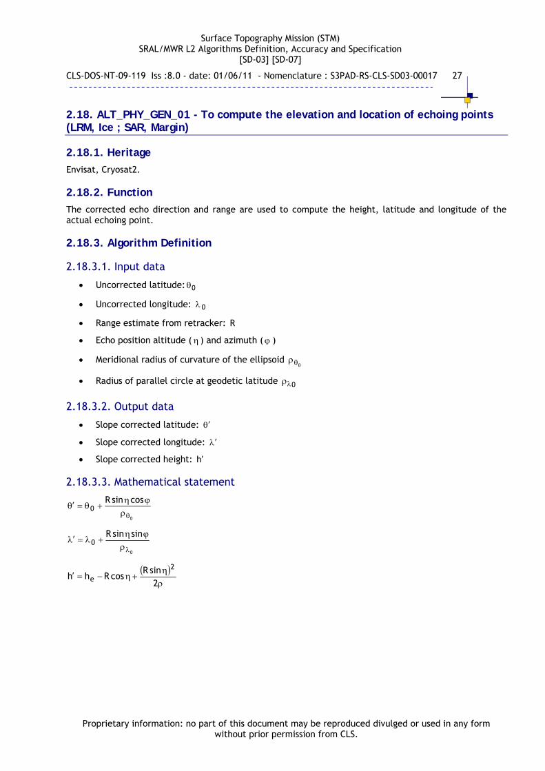
2.18. ALT_PHY_GEN_01 - To compute the elevation and location of echoing points (LRM, Ice ; SAR, Margin)

2.18.1. Heritage

Envisat, Cryosat2.

2.18.2. Function

The corrected echo direction and range are used to compute the height, latitude and longitude of the actual echoing point.



Uncorrected latitude: 0

Uncorrected longitude: 0

Range estimate from retracker: R

Echo position altitude ( ) and azimuth ( )

Meridional radius of curvature of the ellipsoid 0

Radius of parallel circle at geodetic latitude 0


Slope corrected latitude:

Slope corrected longitude:

Slope corrected height: h


0

cossinR0

0

sinsinR0

2

sinRcosRhh

2

e


[SD-03] [SD-07]



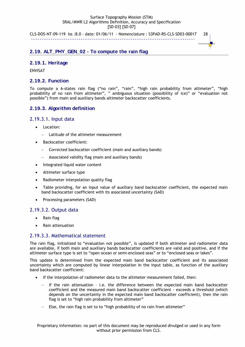
2.19. ALT_PHY_GEN_02 - To compute the rain flag

2.19.1. Heritage

ENVISAT

2.19.2. Function

To compute a 6-states rain flag (“no rain”, “rain”, “high rain probability from altimeter”, “high probability of no rain from altimeter”, ” ambiguous situation (possibility of ice)” or “evaluation not possible”) from main and auxiliary bands altimeter backscatter coefficients.

2.19.3. Algorithm definition


Location:

Latitude of the altimeter measurement


Corrected backscatter coefficient (main and auxiliary bands)

Associated validity flag (main and auxiliary bands)

Integrated liquid water content

Altimeter surface type

Radiometer interpolation quality flag

Table providing, for an input value of auxiliary band backscatter coefficient, the expected main band backscatter coefficient with its associated uncertainty (SAD)

Processing parameters (SAD)


Rain flag

Rain attenuation


The rain flag, initialized to “evaluation not possible”, is updated if both altimeter and radiometer data are available, if both main and auxiliary bands backscatter coefficients are valid and positive, and if the altimeter surface type is set to “open ocean or semi-enclosed seas” or to “enclosed seas or lakes”.

This update is determined from the expected main band backscatter coefficient and its associated uncertainty which are computed by linear interpolation in the input table, as function of the auxiliary band backscatter coefficient:

If the interpolation of radiometer data to the altimeter measurement failed, then:

If the rain attenuation – i.e. the difference between the expected main band backscatter coefficient and the measured main band backscatter coefficient - exceeds a threshold (which depends on the uncertainty in the expected main band backscatter coefficient), then the rain flag is set to “high rain probability from altimeter”

Else, the rain flag is set to to “high probability of no rain from altimeter”


[SD-03] [SD-07]



Else if the rain attenuation exceeds the above-mentionned threshold and if the integrated liquid water content from the radiometer exceeds some given threshold, then:

If the latitude exceeds a given threshold, then the rain flag is set to “ambiguous situation”

Else, the rain flag is set to “rain”

Else, the rain flag is set to “no rain”

The input main and auxiliary bands backscatter coefficients to be used are not corrected for atmospheric attenuation.

(1) Set to "SRAL" or "SRAL+MWR" (2) 4 states (“open ocean or semi-enclosed seas”, “enclosed seas or lakes”, “continental ice”, “land”). (3) Two states : “valid”, or “invalid” (4) 4 states: “good”, “interpolation with gap”, “extrapolation”, or “fail”

(5) Six states : “no rain”, “rain”, “high rain probability from altimeter”, “high probability of no rain from altimeter”, ” ambiguous situation (possibility of ice)” or “evaluation not possible”


[SD-03] [SD-07]



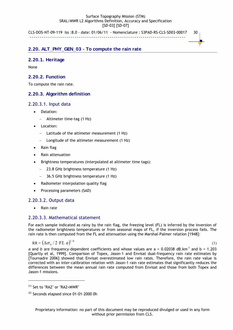
2.20. ALT_PHY_GEN_03 - To compute the rain rate

2.20.1. Heritage

None

2.20.2. Function

To compute the rain rate.



Datation:

Altimeter time-tag (1 Hz)

Location:

Latitude of the altimeter measurement (1 Hz)

Longitude of the altimeter measurement (1 Hz)

Rain flag

Rain attenuation

Brightness temperatures (interpolated at altimeter time tags):

23.8 GHz brightness temperature (1 Hz)





Rain rate


For each sample indicated as rainy by the rain flag, the freezing level (FL) is inferred by the inversion of the radiometer brightness temperatures or from seasonal maps of FL, if the inversion process fails. The rain rate is then computed from the FL and attenuation using the Marshal-Palmer relation [1948]:

RR = baFL /10 2/ (1)

a and b are frequency-dependent coefficients and whose values are a = 0.02038 dB.km-1 and b = 1.203 [Quartly et al, 1999]. Comparison of Topex, Jason-1 and Envisat dual-frequency rain rate estimates by [Tournadre 2006] showed that Envisat overestimated low rain rates. Therefore, the rain rate value is corrected with an inter-calibration relation with Jason-1 rain rate estimates that significantly reduces the differences between the mean annual rain rate computed from Envisat and those from both Topex and Jason-1 missions.

(1) Set to "RA2" or "RA2+MWR" (2) Seconds elapsed since 01-01-2000 0h


[SD-03] [SD-07]



2.21. ALT_PHY_RAN_01 - To compute the retracked altimeter ranges

2.21.1. Heritage

Jason-1, Jason-2, ENVISAT

2.21.2. Function

For each elementary measurement, to compute the retracked estimates of the altimeter range (main and auxiliary bands).



Tracker range:

Tracker range (corrected in the level 1b processing)

Retracking outputs:

Epoch


Universal constants (SAD):

Light velocity


Altimeter range and associated validity flag


For each elementary measurement in main and auxiliary bands, the altimeter range is computed using (1), where ht represents the input tracker range and where is the epoch estimate output by the retracking algorithm.

thh (1)

The validity of the retracked altimeter ranges is determined from the retracking execution flags. Default values are provided in case of invalidity of the retracked altimeter range estimates.

(3) Six states : “no rain”, “rain”, “high rain probability from altimeter”, “high probability of no rain from altimeter”, ” ambiguous situation (possibility of ice)” or “evaluation not possible” (4) 4 states: “good”, “interpolation with gap”, “extrapolation”, or “fail”


[SD-03] [SD-07]



2.22. ALT_PHY_RAN_02 – To compute the surface height anomaly (SAR, Sea-Ice)

2.22.1. Heritage

Cryosat2

2.22.2. Function

Provide a surface height anomaly relative to the mean sea surface and corrected for retracker height error and other effects.



Platform altitude: eh

Range corrected for fitting retracker: fitR

Mean sea surface: MSSh


Surface height: h

Sea surface height anomaly: shah


The surface height is calculated as fite Rhh

This gives the surface height anomaly MSSsha hhh


[SD-03] [SD-07]



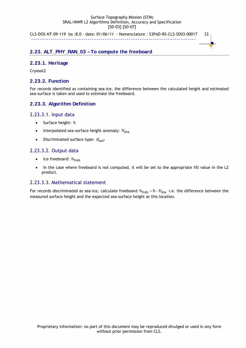
2.23. ALT_PHY_RAN_03 – To compute the freeboard

2.23.1. Heritage

Cryosat2

2.23.2. Function

For records identified as containing sea-ice, the difference between the calculated height and estimated sea-surface is taken and used to estimate the freeboard.



Surface height: h

Interpolated sea-surface height anomaly: shah

Discriminated surface type: surfd


Ice freeboard: frebh

In the case where freeboard is not computed, it will be set to the appropriate fill value in the L2 product.


For records discriminated as sea-ice, calculate freeboard shafreb hhh i.e. the difference between the

measured surface height and the expected sea-surface height at this location.


[SD-03] [SD-07]



2.24. ALT_PHY_SNR_01 - To compute the SNR from the estimates of the amplitude and of the thermal noise level of the waveforms

2.24.1. Heritage


2.24.2. Function

To compute the signal to noise ratio (main and auxiliary bands) from the estimates of the amplitude and of the thermal noise level of the waveforms.




AGC:

Corrected AGC: AGCc

Retracking outputs (power):

Amplitude of the waveforms (Pu ) and associated validity flag

Thermal noise level of the waveforms (Pn) and associated validity flag


Minimum value of AGC requested to set SNR to AGC in case of null thermal noise: AGCmin

Bias between SNR and AGC: Bias


Signal to noise ratio


For each band, the signal to noise ratio is computed by:

n

u10 P

Plog.10SNR (1)

The input validity flags are managed. Moreover, if the thermal noise level is set to 0, the signal to noise ratio is set to AGCc + Bias (if AGCc exceeds a threshold, AGCmin), or otherwise to Pu (in dB) (i.e. that Pn is set to the amplitude resolution of the analysis window).



[SD-03] [SD-07]



2.25. ALT_PHY_SWH_01 - To compute SWH from the retracked composite Sigma

2.25.1. Heritage

Jason-1, ENVISAT, Jason-2

2.25.2. Function

For each elementary measurement, to derive the estimates of the significant waveheight (main and auxiliary bands) from the retracked estimates of the composite Sigma.




Retracking outputs (composite Sigma):

Composite Sigma



Sampling interval of the analysis window

Ratio between the PTR width and the sampling interval of the analysis window


Light velocity




For each elementary measurement in main and auxiliary bands, the significant waveheight SWH is computed as follows:

2p

2c.c2SWH (1)

where: c is the composite Sigma (expressed in time units) p is the PTR width (expressed in time units) c is the light velocity

The validity of the significant waveheights is determined from the retracking execution flags.



[SD-03] [SD-07]



2.26. ALT_PHY_WIN_01 - To correct the backscatter coefficients for atmospheric attenuation and to compute the 10 meter altimeter wind speed

2.26.1. Heritage

GEOSAT, TOPEX/POSEIDON, ERS-1, ERS-2, ENVISAT

2.26.2. Function

To correct the backscatter coefficients for atmospheric attenuation and to compute the altimeter wind speed from the corrected Ku-band backscatter coefficient and the Ku-band significant waveheight.




Ku-band ocean backscatter coefficient

C-band ocean backscatter coefficient

Ku-band ocean backscatter coefficient validity flag

C-band ocean backscatter coefficient validity flag

Atmospheric attenuation:

Ku-band backscatter coefficient atmospheric attenuation

C-band backscatter coefficient atmospheric attenuation

Backscatter coefficient to wind speed conversion (SAD, look-up table)


Backscatter coefficients (both bands) corrected for atmospheric attenuation

Wind speed corrected for atmospheric attenuation


First, atmospheric attenuation is added to the backscatter coefficient to correct it (in both bands). Then the wind speed is computed (in m/s) from a model depending on the Ku-band corrected backscatter coefficient.


[SD-03] [SD-07]



2.27. ALT_RET_ICE_01 – To perform the ice-1 (OCOG) retracking (SAR sea-ice, margin ; LRM ice)

2.27.1. Heritage

Envisat, Cryosat2.

2.27.2. Function

A standard OCOG retracking is performed on the power waveform.

The OCOG retracking method is the same for all forms of this algorithm, however the processing parameters may be tuned independently. This tuning is performed by loading a set of processing parameters that are appropriate to the mode and surface type.



Power waveform: 1N:0P s

trR tracker range from L1b

CoG correction CoGd

Applicable geophysical and meteorological corrections C


bind size of a range window bin in metres

TPi nominal tracking point


OCOG Retracker range correction : OCOGR

OCOG Retracker range estimate : OCOGR

OCOG Retracker power estimate : OCOGP


Calculate OCOG amplitude as

1N

0i

2

1N

0i

4

OCOGs

s

]i[P

]i[P

P

Search the power waveform array to locate the index of first bin containing more power than

OCOGP as 0i

Calculate OCOG retrack bin 1iPiP

1iPP1ii

00

0OCOG0OCOG


[SD-03] [SD-07]



The OCOG range correction is binTPOCOGOCOG diiR

Calculate the OCOG corrected range as CoGOCOGtrOCOG dCRRR


[SD-03] [SD-07]



2.28. ALT_RET_ICE_02 - To perform the ice-2 retracking (LRM)

2.28.1. Heritage

ENVISAT, Jason-2

2.28.2. Function

To perform the ice-2 retracking (the so-called ice_erf algorithm) on the waveforms.



Altimeter configuration data and quality information

Waveform:

Waveform (128 FFT samples for Ku and C bands)


Altimeter instrumental characterization data for the preparation of data for the ice-2 retracking




Light velocity


For each band, the following 20-Hz parameters:

Epoch or "range offset":

Width of the leading edge: L

Amplitude: Pu

Mean amplitude: Pt

Thermal noise level: Pn

Slope of the first part of the logarithm of the trailing edge: sT1

Slope of the second part of the logarithm of the trailing edge: sT2

Slope of the first part of the logarithm of the trailing edge for mispointing estimation: sT1m (Ku band only)


Mean quadratic error between the normalized waveform and its model

Quality information, such as an execution flag (valid / invalid)


[SD-03] [SD-07]




The ice-2 retracking algorithm is performed on the Ku and on the C band waveforms. The only difference in the retracking of Ku and C waveforms is the processed data (waveform, processing and instrumental parameters). A single description is thus given below.

Background

The ice-2 retracking algorithm is based on the ENVISAT RA-2 ice-2 retracking. The aim of the ice-2 retracking algorithm is to make the measured waveform coincide with a return power model, according to Least Square estimators.

The expression of the return power as a function of time is given Brown (Brown, 1977):

nTL

u Pt.sexp.t

erf1.2

P)t(Vm

(with:

x

0

t dte.2

)x(erf2

) (1)

where the parameters to be estimated are:

: the epoch

L : the width of the leading edge

Pu : the amplitude

sT : the slope of the logarithm of the trailing edge

Pn : the thermal noise level (to be removed from the waveform samples)

Basic principle and main steps of the processing (see RD 3)

The basic principle and the main steps of the processing are defined hereafter.

Identification of the waveform validity:

The validity of the waveform is determined from the input waveform quality information. The retracking is then performed only if the input waveform is valid.

Waveform normalization and leading edge identification:

Depending on the option for thermal noise determination (processing parameter), the thermal noise level (Pn) is either the input noise power measurement (NPM), or it is computed from an arithmetic average of samples of the first plateau, or it is a default value (processing parameter).

Pn is removed from the waveform samples which is then normalized (i.e. divided by an estimate of the maximum amplitude of the useful signal). Finally, the beginning and the end of the leading edge are identified from an analysis of the shape of the waveform (accounting in particular for the frequent case of a trailing edge with a positive slope), and an estimation window is built around the detected leading edge.

Coarse estimation stage (, L):

A coarse estimation of the epoch () of the waveform in the estimation window and of the width of the leading edge (L), is then derived from Least Square estimators by fitting the processed waveform to a mean return power model with a flat trailing edge. This fit is performed in the estimation window i.e. around the leading edge of the waveform. These estimates are the values which minimize the residual in the estimation window, between the normalized waveform and the corresponding model. For each possible value of (corresponding to a position varying between the beginning and the end of the estimation window, with a predefined step) and of L (varying between two thresholds, with a predefined step):

The normalized model (Vmn) is computed in the estimation window


[SD-03] [SD-07]



The amplitude Pu of the normalized waveform is estimated by minimizing the mean quadratic error between the normalized waveform (Vn) and the weighted normalized model (Pu.Vmn) in the estimation window (linear regression between the waveform and the normalized model)

The residual R between Vn and Pu.Vmn is computed in the estimation window

The estimates are updated if R is smaller than the previous minimum value

Fine estimation stage (, L, Pu):

A fine estimation of , L and Pu (amplitude) is finally derived. The coarse and fine estimation stages are very similar. The particularities of the fine estimation process are the following: the simulated values of andL correspond to a position and a width, centered on the coarse estimates, with left and right deviations equal to the half of the coarse resolutions, and with predefined steps (smaller than those used in the coarse estimation process).

The estimated amplitude is provided in output.

Estimation of the slope of the logarithm of the trailing edge (sT1, sT2):

The estimation of the slope of the logarithm of the trailing edge is intentionally fully decorrelated from the estimation of the other parameters (, L, Pu), because slopes variations may be very important from a waveform to another, and because the uncertainty on its estimate is very important due to speckle effects. Indeed, over ice surfaces, the slope of the trailing edge depends on several parameters among which the slope and the curvature of the overflown surface, the signal due to the penetration of the radar wave in the snow pack (Legresy and Remy, 1997), and of course instrumental features (e.g. antenna). The slope is estimated by linear regression of the logarithm of the normalized waveform samples in two windows part of the trailing edge: the first one (sT1) just after the end of the leading edge with a predefined width, and the second one (sT2) in a contiguous window with a predefined width. The first estimation is aimed at pointing out a possible volume signal existing at the end of the leading edge.

For Ku band, a third slope (sT1m) is estimated as sT1, with an other predefined width aimed at pointing out a mispointing angle over ocean surfaces.

Estimation of the mean amplitude (Pt):

The mean amplitude of the waveform is estimated by an arithmetic average of the waveform samples (thermal noise level removed) in a window limited by the beginning of the leading edge and the end of the first window used in the slope estimation.

Finally, outputs are converted (the epoch is referred to the analysis window, the amplitude Pu is denormalized, etc.)

(1) Value to be selected according to the processed band, the emitted bandwidth and the operating RF subsystem (Ku bandwidth and RF subsystem identifiers) (2) Values to be selected according to the processed band and the emitted bandwidth (Ku bandwidth identifier)


[SD-03] [SD-07]



2.29. ALT_RET_ICE_03 – To perform the “function fit” retracking (SAR, Sea-Ice)

2.29.1. Heritage

Cryosat2

2.29.2. Function

The power waveform is retracked by fitting a function that models the expected power return to the waveform.

The retracking method is the same for both the sea-ice and ice-sheet forms of this algorithm, however the processing parameters may be tuned independently.





CoG correction CoGd





Initialisation values for function parameters (may be static from configuration files or dynamic from prior waveform QA or OCOG retracking): 1N:0

Amplitude 0a0

Tracking point 1t0 ( fiti when expressed in bins)

Sigma of Gaussian 2

Exponential 3k

iterN maximum number of iterations to perform

2finish stop iterating if the fit converges to this level

iterr stop iterating if the improvement in the fit is less that this ratio

stuckN stop iterating if the fit does not improve for this many consecutive iterations


Final (fitted) value of function parameters: 1N:0

Retracker waveform power estimate: fitP

Retracker range correction: fitR


[SD-03] [SD-07]



Retracker range estimate: fitR

Retracker quality measurement: 2fit


Fit ,tftP by non-linear least-squares method (Levenberg-Marquard).

The fitted function ,tf is a three-part piecewise function:

Leading edge

20tt

01 ea,tf

Linking function

2

02

0b

302

b

tt1

ttct2

c4k5tt

ct2

c2k3

02 ea,tf

, where

2b kt

bktc

Trailing edge 0ttk03 ea,tf

tt

ttt

tt

for

for

for

)t(P

)t(P

)t(P

tP

b

b0

0

3

2

1

(note that 0t and bt

are defined above)

The range correction for the fitted retracker is

binTPfitfit diiR

The range corrected for the fitted retracker is CoGfittrfit dCRRR


[SD-03] [SD-07]



2.30. ALT_RET_ICE_04 - To merge MLE4 results into the ice chain (LRM Ice)

2.30.1. Heritage

2.30.2. NoneFunction

Usage of the CryoSat retracker CFI has been removed as the software is no longer supported. The functionality will be replaced by using the results of the MLE4 retracker (which are read from the input L2 file). This algorithm now simply maps the MLE4 results onto the variables previously filled by the CFI retracker.

The processing is described below.



CoG correction CoGd


MLE4 retracking ‘epoch’: 4MLER

MLE4 power estimate: 4MLEP


MLE4 Retracker range estimate: RCFI

MLE4 power estimate: CFIP


Calculate the MLE4 corrected range as CoGMLEtrCFI dCRRR 4


[SD-03] [SD-07]



2.31. ALT_RET_ICE_05 - To perform the SAR ice-margin WW retracking (SAR ice margin)

2.31.1. Heritage

Cryosat2.

2.31.2. Function

A model of the SAR mode waveform is fitted to the received power. The amplitude and retracking offset are derived from analysis of the fitted waveform. The method is that used for waveforms received in the SARin degraded case for CryoSat where the phase and coherence information is unavailable.





CoG correction CoGd






WW Retracker range correction: WWR

WW Retracker range estimate: WWR

WW Retracker power estimate: WWP


The retracking algorithm has been designed to exploit least squares fitting of a semi-analytical model of the echo. The echo model is a modified gaussian of the form:

tfaetP

where f is a 5-part piecewise continuous function whose form addresses different regions of the

echo thus:

ntt wherentgmttgtf 0001

203

1032

10210102 tttnt wherett-tbtt-tbtt-tbbtf

102010

3 ttttt wherettt

1tf


[SD-03] [SD-07]



30103

1032

102104 ttttt wherett-tatt-tatt-t1

tf

30

21

0

tt

5 ttt wheretta

celogtf

0

A Levenberg-Marqhart non-linear least-squares fit is performed to derived the parameters t,c,n,,,a . Then:

)Pmax(aPWW

TPbinWW itdR

CoGWWtrWW dCRRR


[SD-03] [SD-07]



2.32. ALT_RET_OCE_01 - To perform the ocean retracking (LRM)

2.32.1. Heritage

Jason-2

2.32.2. Function

To perform the ocean retracking (hereafter called “ocean-3” retracking from Jason heritage) on the waveforms (main and auxiliary bands), i.e. to estimate the altimetric parameters (epoch, composite Sigma, amplitude, square of the mispointing angle).

In this algorithm, the resolution of the set of m linear equations is based on a least-square method and utilizes the standard routine “F04AMF” of the NAG library, simulated by the routines “dgeqrf” and “dormqr” from the public LAPACK library (www.netlib.org/lapack) and the routines "dtrsm", "dgemv" and "dnrm2" from the BLAS library (www.netlib.org/blas). Thus, a wrapper (provided by CLS) will be used to call these routines with the interfaces expected from the “F04AMF” routine of the NAG library.




Waveform:

Waveform

Waveform validity flag

Off-nadir angle:

Off-nadir angle (square value)

Orbit:

Orbit altitude (20-Hz)


Altimeter instrumental characterization data for the preparation of data for the ocean retracking

Abscissa of the reference sample for tracking


Antenna beamwidth

Ratio between the PTR width and the sampling interval of the analysis window



Light velocity

Earth radius


For each band, the following 20-Hz parameters:


[SD-03] [SD-07]



Epoch:

Composite Sigma: c

Amplitude: Pu


Square of the mispointing angle: 2 (relevant for Ku-band only)

Mean quadratic error between the normalized waveform and its model

Number of iterations

Quality information, such as an execution flag (valid / invalid)


The ocean-3 retracking algorithm is performed on the Ku-band and on the C-band waveforms. For each 20-Hz measurement, the Ku-band waveform must be processed first, because the Ku-band estimate of the square of the mispointing angle is requested on input of the processing of the C-band waveform.

Background

The aim of the ocean-3 retracking algorithm is to make the measured waveform coincide with a return power model, according to weighted Least Square Estimators derived from Maximum Likelihood Estimators. Regarding mispointing, the return power model accounts for the second order terms. Moreover, within the Ku-band ocean-3 retracking, the square of the off-nadir angle is estimated together with the three standard altimetric parameters (epoch, composite Sigma and amplitude).

The expression of the return power as a function of time is given by Amarouche (Amarouche, 2003). Accounting for a skewness coefficient (s: processing parameter), and assuming a Gaussian Point Target Response, it is given by:

n222

3c

322

3

c

ss22

u

211

3c

311

3

c

ss11u

Puexpw2

uerf16

uerf1vexp2

PA

uexpw2

uerf16

uerf1vexpAP)t(Vm

(1)

with:

x

0

t dte.2

)x(erf2

2sin4

expA , )2

(sin.)2(Log

2 02

e

, o = antenna beamwidth

2sin.

R

h1h

c.

4

e

,

2cos.

R

h1h

c4

e

, 8

2

1

, 2

with: c = velocity of light, h = mean (raw) satellite altitude, Re = earth radius

p = PTR width (expressed in time), sc2SWH (significant waveheight), 2s

2p

2c

c

2c1

12

tu

,

2tv

2c1

11 , 13u23u2w 2c

211c1

211


[SD-03] [SD-07]



c

2c2

22

tu

,

2tv

2c2

22 , 13u23u2w 2c

222c2

22 2

and where the parameters to be estimated are:

: the epoch

c : the composite Sigma

Pu : the amplitude

: the mispointing angle (Ku-band only)

Pn : the thermal noise level (estimated from an arithmetic average of samples of the first plateau)

Basic principle

The problem to solve is the estimation of a set of N=4 parameters ={1=,2=c,3=Pu,4=2} for Ku-band, and N=3 parameters ={1=,2=c,3=Pu} for C-band. The system to solve results from the maximization of the logarithm of the likelihood function (), i.e. from the system:

0)(Ln)(C (2)

where C is the total cost function and is the gradient function.

This system is reduced to weighted Least Square Estimators, and is equivalent to set the Least Square function 2 to 0, where the merit function 2 is defined by:

2

i i

ii2 Vm_V

(3)

where V represents the measured waveform, and where the weighting function is {i} = {Vmi}.

This system may also be represented by the following set of N equations:

0Vm

.VVm

k

i

i2i

ii

(4)

An iterative solution is obtained by developing the total cost function in a Taylor series at the first order about an initial set ={01=,02=c0,03=Pu0,40=2

0} of estimates (for C-band, 40 is the Ku-band estimate of the square of the mispointing angle, and the square of the mispointing angle is not estimated) :

.gn1n (5)

with: BD)BB( 1T (valued to the current values n)

k

i

iik

Vm.

1B

, ii

i1i VVm.

1D

and where g is a loop gain (positive value, unique to the parameter being estimated).

Using {i} = {Vmi}, the Least Square Estimators method described above would put the most weight on the regions with the least power, i.e. on the regions with the least information regarding the parameters to be estimated. For this reason, the weighting function is superseded by a factor constant over a waveform ({i} = ). In order to normalize the residuals ({Vmi-Vi}), this factor is set to the current estimate of the amplitude.

Main steps of the processing


[SD-03] [SD-07]



The main steps of the nominal processing are the following:

Identification of the waveform validity:

The validity of the waveform is determined from the input waveform quality information. The retracking is then performed only if the input waveform is valid.

Thermal noise estimation:

The thermal noise level (Pn) is computed from an arithmetic average of samples of the first plateau (in a predefined gate).

Initialization:

A default value of the epoch (processing parameter) is used when the instrument is operating in closed loop, while this default value is superseeded by the estimate of the epoch output by “ALT_MAN_RET_04 - To initialise the LRM ocean retracking” for the processed band when the instrument is operating in closed loop.

Estimation (weighted Least Square fit):

The fine estimates of the epoch (), the composite Sigma (c), the amplitude (Pu) and for the Ku-band the square of the off-nadir angle (2), are derived from the iterative process defined previously, which is initialized from default values , c0, Pu0 and 2

0 (input processing parameters, except 2

0 for C-band, which is the Ku-band estimate of the square of the mispointing angle) for each waveform.

This estimation process is stopped when the value of the mean quadratic error between the normalized waveform (i.e. the waveform from which Pn is removed and weighted by 1/Pu) and the corresponding model built from the estimates is stable enough, with a minimum number of iterations performed, or when a maximum number of iterations is reached.

(1) Value to be selected according to the processed band (5) Square_Mis_IN is used only if the mispointing option (processing parameter) is set to "No Estimation" (4) Min_Iter is greater or equal to 2 (6) 2 states: "Estimation" (the square of the mispointing angle is estimated) or "No Estimation" (the square of the mispointing angle is not estimated) (7) Relevant only if the mispointing option (processing parameter) is set to "Estimation", otherwise the output is set to the input value (Square_Mis_In) in the processing (8) M=4 if Mis_Option is set to "Estimation", M=3 if Mis_Option is set to "No Estimation" (1) 3 states: "Model", "Derivatives" or "Model and Derivatives" (2) 2 states: "Estimation" or "No Estimation"


[SD-03] [SD-07]



2.33. ALT_RET_OCE_02 - To perform ocean/coastal zone retracking (SAR)

2.33.1. Heritage

None

2.33.2. Function

To fit the theoretical multi-looked waveform model to one 20-Hz Level 1B SAR waveform using the Levenberg-Marquardt method and to retrieve geophysical variables and fitting quality information.



L1b SAR mode waveforms

Universal constants

Instrumental characterization data



Epoch relative to central gate position

RMS height of specular points with reference to MSL

Maximum Received Power

Squared Mispointing Angle

Inverse of the variance of ocean surface total slope (1/MSS)

Abscissa of first WF sample for which to compute the theoretical DDM

Abscissa of last WF sample for which to compute the theoretical DDM

Thermal noise

Least square fitting routine exit flag

Number of iterations on exiting least square fitting loop

Sum of squared residuals on exiting least square fitting loop


The algorithm consists of the following functional units:

An initialisation unit, INIT, which checks various flags and prepares the waveform measurements according to the specification set by the user in the processing parameters related to INIT.

A fitting unit, FIT, which performs the least-square fitting of the SAMOSA theoretical SAR waveform model to the measured waveforms, according to the specification set by the user in the FIT related processing parameters.

The fitting unit relies on two mechanisms (i.e., functional units) to perform the computation of, respectively, the single-look (SL) and multi-look (ML) theoretical waveforms. The SL unit depends


[SD-03] [SD-07]



solely on input data, while the ML unit is also controlled through the processing parameters of the ML mechanism.

The overall structure of the algorithm is illustrated in Figure 2.

Figure 2 - SAR ocean retracker global software structure

Mathematical assumptions for the derivation of the analytical expression of the Single-Look Model

The analytical expression of the Single-Look Model is derived from convolving three terms:

W , fa PFS , fa SR , fa c

2

Pz

c2

(1)

The flat surface impulse response, PFS , fa , the radar system point target response SR , fa and the


[SD-03] [SD-07]



surface probability density function, Pz . The system point target response is composed of two squared sinc functions, both approximated by Gaussian functions for simplification.

SR , fa sinc2 T fa sinc2 su (2)

SR , fa exp fa

2

2 v2

exp

2

2 p2

(3)

p p

Br

prB (4)

v p

1

T (5)

We have used Least Squares (LS) to do such approximation, achieving a perfect fit in the main lobe of the sinc2 by a Gaussian function when p 0.366.

rB corresponds to the time resolution defined by the receiver bandwidth.

rB =1

BW (6)

and T corresponds to the along-track boxcar (Na/PRF, where Na is the number of echoes per burst). Single-Look Model

The single-look model analytical expression for no across-track curvature effects and no across-track mispointing angle is given by:

W (, fa ) W0 exp fa a 2

2 a2

exp

( m 2)2

4 2 m m 2 /2

m 2

2 c /hK1/ 4

14 2

m 2 2

m 2 0

m 2

2 c /hI1/ 4

1

4 2 m 2 2

I1/ 4

1

4 2 m 2 2

m 2 0

(7)

where I and K are the modified Bessel functions of the first (I) and second (K) kind. The variables in the equation above are described in the table below.

The single-look model in Eq. 7 is a 2D matrix representing the distribution of power in Delay and Doppler space (hence, Delay-Doppler Maps; DDM).


[SD-03] [SD-07]



Symbol Single-look Model Variables Equation Label Units

Range gate or delay time with respect mean sea level (related to the epoch)

t t0 (8) [s]

f a Doppler bin, or Doppler frequency (each scatterer is related to an along-

track position xa; x0corresponds to the altimeter along track position [Raney, 1998]

fa 2Vs

0hx0 xa (9) [Hz]

W 0 Single-looked model amplitude factor (see section 3.4.2.1) (10) [Watts/s]

a Along-track mean that results from applying FFT a

2Vs

0 2 cos2 sin2

(11) [Hz]

v Standard deviation derived from approximating the radar system point target response along-track sinc2 by a Gaussian function

v2

p

T

2

(12) [Hz2]

b Standard deviation from the along-track flat surface impulse response b

2 2 2Vs

2

02 2 cos2

(13) [Hz2]

a Standard deviation that result from convolving the system flat surface impulse response and the radar point target response along-track

a2 v

2 b2

(14) [Hz2]

m Variable related to mispointing angle and MSS m

c

h 2 cos2 (15) [Hz]

Standard deviation derived from the convolution of the ocean surface p.d.f and the system point target response

2 prB 2 2 s

c

2

(16) [s2]

Single-Look model variables

Amplitude factor Wo

The amplitude factor multiplying is given by:

W0 Pu exp 2 sin2 2

2 cos2 sin2 2

(17)

Pu PtG02 0 0 0

3c

4 4 2L ph

3Vs

1

21

prB v b

1

a

(18)

Multi-Look Model

For the generation of the multi-look waveforms we need to account for: Neff and Beam_Ang_Stack_TS; both are provided for each elementary record (approximately 20-Hz waveform) in the SAR L1b product.


[SD-03] [SD-07]



Neff corresponds to the number of effective looks for a given elementary record. This number represents the number of looks used for multi-looking at the present ground cell location. Neff can differ from the maximum number of looks available in principle, because some looks may not be suitable due to low Signal to Noise Ratio (SNR).

Beam_Ang_Stack_TS is the array of angles of the Doppler beams used for multi-looking for the given elementary record. It provides in radians the value of the angle of all beams staring at the ground resolution cell. This array can be easily related to the Doppler frequency of each effective burst bin used for multi-looking.

First, we will calculate for each angle in Beam_Ang_Stack_TS, the corresponding Doppler frequency:

Dopp_Freq_Stack_TS(n) 2Vs

0

cos(Beam_Ang_Stack_TS(n)) 1 n Neff (19)

This will define the Doppler bins of each burst that must be selected and added to the stack before incoherent integration. The final expression for the multi-looked waveform is given by:

WML W , Dopp_ Freq_ Stack _TS(n) n1

Neff

(20)


[SD-03] [SD-07]



2.34. GEN_COR_ORB_01 - To derive the orbital altitude rate with respect to the reference MSS/geoid

2.34.1. Heritage

Jason-1, Jason-2

2.34.2. Function

To derive the orbital altitude rate with respect to the MSS/geoid from the orbital altitude rate with respect to the reference ellipsoid and from the map of slopes of the MSS/geoid with respect to the reference ellipsoid.



Pass:

Pass number of the measurement (indicating if the pass is ascending or descending)

Location:

Latitude

Longitude

Orbit:

Orbital altitude rate with respect to the reference ellipsoid

Map of the slopes of the reference MSS/geoid with respect to the reference ellipsoid (SAD)


Orbital altitude rate with respect to the reference MSS/geoid


The orbital altitude rate with respect to the reference MSS/geoid is the sum of the two following parameters:

The input orbital altitude rate with respect to the reference ellipsoid

The slope of the reference MSS/geoid with respect to the reference ellipsoid, which is derived by bilinear interpolation of the slopes of the input map to the measurement location, accounting for the pass direction (ascending or descending).

(1) Two values are provided for each point of the grid: one for the ascending passes, the other for the decending passes


[SD-03] [SD-07]



2.35. GEN_COR_RAN_01 - To compute the 10 meter wind vector, the surface pressure and the mean sea surface pressure from ECMWF model, the dry and wet tropospheric “operational” corrections (ocean surfaces) and the dry and wet tropospheric “pseudo-operationnal” corrections (continental surfaces)

2.35.1. Heritage

Jason-1

2.35.2. Function

To compute at the altimeter time tag and location the 10 meter wind vector components U (zonal component) and V (meridian component), the surface pressure and mean sea level pressure from the ECMWF meteorological model fields, the wet tropospheric corrections due to gases of the troposphere (ocean surfaces), to remove the climatological pressure from the surface pressure and to derive the dry tropospheric corrections due to gases of the troposphere from this surface pressure to which a model of S1 and S2 pressure variability is added (ocean surfaces), to compute the wet and dry tropospheric corrections using a vertical integration of the meteo 3D parameters (continental surfaces).



Datation:

Altimeter time tag

Location:

Latitude of the measurement

Longitude of the measurement

Altitude

Tracker range

Geophysical corrections

Meteorological data (DAD):

Meteorological data: U and V components of the 10 meter wind vector, surface pressure and mean sea level pressure. For each of these parameters, the data consist of two data files, 6 hours apart, bracketing the time of measurement (each file, excepted the mean sea surface pressure, contains the parameter given on the so-called Gaussian grid (quasi-regular in latitude, non-regular in longitude).

Humidity and temperature profiles from the vertical levels

Table providing the latitudes of the model grid points

Table providing the number of grid points in longitude for each model latitude

Climatological pressure files (SAD)

The data consists of four data files, corresponding to 0h, 6h, 12h and 18h. Each file contains the climatological pressure referenced to the sea on a cartesian grid, for each of the twelve months of the year.

S1 and S2 tide grids of monthly means of global amplitude and phase (SAD)


[SD-03] [SD-07]





U-component of the 10 meter model wind vector

V-component of the 10 meter model wind vector

Dry tropospheric “operational” and “pseudo-operational” corrections: hdry and hdry-pseudo

Model wet tropospheric “operational” and “pseudo-operational” corrections: hwet and hwet-pseudo

Surface pressure (climatological pressure removed)

Mean sea level pressure


The wet tropospheric correction, the two components U and V of the 10 meter model wind vector, the surface pressure and the mean sea surface pressure at the altimeter measurement are obtained by linear interpolation in time between two consecutive (6 hours apart) ECMWF model data files, and by bilinear interpolation in space from the four nearby model grid values (excepted for the mean sea surface pressure). The ECMWF model grid is quasi-regular in latitude and non-regular in longitude (the number of grid points in longitude increases towards lower latitudes).

The climatological pressure (0h, 6h, 12h and 18h for each month) is then removed from the surface pressure.

Then, the dry/wet tropospheric corrections are computed as follows :

“operational corrections” : both corrections described below are computed at the “sea level reference” so that coastal points do not suffer from interpolation between ocean and continental points corrections, the drawback being that the non ocean points will be affected with unrealistic values :

The dry tropospheric correction is derived from the mean sea level pressure (climatological pressure removed) to which a model of S1 and S2 pressure variability (R D Ray and R M Ponte, 2003) is added.

The wet troposhperic correction is computed from a “surface“ reference that is the mean sea level pressure and the calculation is based on equation (21) described below.

“pseudo-operational corrections” : for both corrections, the computation consists in a vertical integration of the 3D meteo parameters performed for each along-track altimeter measurement. The real altitude of the surface terrain along-track is deduced from the altimeter range. This surface altitude is then used inside the 3D meteo fields in order to determine the altitude of the real surface within the model:

The dry tropospheric correction is computed from equation (15) described below, which requires a value of the surface pressure at the real surface altitude and a value of the gravity at the altitude/latitude of the measurement point for each model layer.

The wet tropospheric correction is computed from equation (21) described below, whoch requires a value of the surface pressure at the real surface altitude, a value of the gravity at the altitude/latitude of the measurement point for each model layer and a value of specific humidity and temperature (given by the 3D ECMWF meteo fields) for each model layer.

Hereafter are detailed the mathematical statement to compute the surface pressure map and the wet tropospheric correction map. The input data for computing these maps are the model surface pressure, and the specific humidity and temperature profiles from the vertical levels of the ECMWF model.

Definitions of the refractive index and of the wet and dry tropospheric corrections


[SD-03] [SD-07]



The excess propagation path, also called path delay, induced by the neutral gases of the atmosphere between the backscattering surface and the satellite is given by:

h = dz 1) - (n(z)Hsat

Hsurf (1)

where n(z) is the index of refraction of air, Hsurf and Hsat are respectively the altitudes of the surface and of the satellite above mean sea level.

The index of refraction is conveniently expressed in terms of the refractivity N(z), defined as:

10-6 N(z) = n(z) - 1 (2)

N(z) is given by Bean and Dutton (1966):

N(z) = 77.6 T

Pd + 72 T

e + 3.75 105

2T

e (3)

where Pd is the partial pressure of dry air in hPa (1 hPa = 100 Pa), e is the partial pressure of water vapor in hPa, and T is temperature in K.

As the partial pressure of dry air is not easily measured, it is desirable to obtain an expression function of the total pressure of air. For deriving it, we have to consider that the dry air and the water vapor are ideal gases, i.e., they obey to the Mariotte-Gay Lussac law:

For dry air: dd

d

M

RT

ρ

P (4)

For water vapor: ww M

RT

ρ

e (5)

where d and w are the volumic masses of dry air and water vapor respectively, Md and Mw are the molar masses of dry air (28.9644 10-3 kg) and water vapor (18.0153 10-3 kg) respectively, R is the universal gas constant (8.31434 J.mole-1.K-1).

Combining (4), (5) and (3) leads to:

N(z) = 77.6 Rd

d

M

ρ + 72 R

w

w

M

ρ + 3.75 105

2T

e (6)

The volumic mass of wet air is the sum of the volumic masses of dry air and water vapor:

= d + w (7)

Introducing the volumic mass of wet air given by (7) into (6) leads to:

N(z) = 77.6 RdM

ρ + (72 - 77.6

d

w

M

M) R

w

w

M

ρ + 3.75 105

2T

e (8)

Reintroducing (5) into (8) leads to the final expression of refractivity N(z):

N(z) = 77.6 RdM

ρ + (72 - 77.6

d

w

M

M)

T

e + 3.75 105

2T

e (9)

Combining this expression with (1) and (2) leads to the following equation for h:

h = 77.6 10-6 dM

Rdz

Hsat

Hsurf + (72 - 77.6

d

w

M

M)10-6 dz

T

eHsat

Hsurf + 3.75 10-1 dz

T

eHsat

Hsurf2 (10)


[SD-03] [SD-07]



The first term is called the dry tropospheric correction hdry:

hdry = 77.6 10-6 dM

Rdz

Hsat

Hsurf (11)

The sum of the two remaining terms is called the wet tropospheric correction hwet:

hwet = (72 - 77.6 d

w

M

M)10-6 dz

T

eHsat

Hsurf + 3.75 10-1 dz

T

eHsat

Hsurf2 (12)

Introducing the numerical values for Md and Mw into (12), and multiplying hwet by –1 to get a negative quantity to be added to the altimeter range, leads to the following equation for hwet in m:

hwet = -23.7 10-6 dz T

eHsat

Hsurf - 3.75 10-1 dz

T

eHsat

Hsurf2 (13)

Calculation of the dry tropospheric correction as function of the surface pressure

It is commonly assumed that the atmosphere is in hydrostatic equilibrium, i.e. g being the acceleration due to gravity:

dz

dP= - g (14)

Combining (11) and (14) leads to the following equation for hdry, where Psurf is the atmospheric pressure at the ground surface:

hdry = 77.6 10-6 dM

R dP

g

1Psurf

0 (15)

The acceleration of gravity is a function of latitude and altitude. This function can be modeled by:

z 0.00031 - )cos(2 0.0026 - 1.gg 0 (16)

where is the latitude, z is altitude in km, and g0 = 9.80665 m/s2

The variation of g with altitude is small and can be neglected by considering a mean value for g = 9.783 m/s2 constant with altitude. This leads to the final expression for hdry:

)2cos(0026.01.P 277.2h urfsdry (17)

(17) is the expression obtained by Saastamoinen (1972), where Psurf is in hPa, and hdry is in mm and is set here with a negative sign to be added to the altimeter range. Computing the dry tropospheric correction from (15) instead of from (17) (i.e., taking into account the variation of g with altitude, as given by (16)), leads to differences below the 1-mm level in dry tropospheric correction (below the 0.5-mm level for latitudes less than 50°).

Note In GEN_COR_RAN_01 algorithm, the dry tropospheric correction will be computed as described in (17) but using a surface pressure which is the interpolated surface pressure Psurf from which the climatological pressure is removed (over the ocean only) and to which a model of S1 and S2 waves pressure variability (R D Ray and R M Ponte, 2003) is added.


[SD-03] [SD-07]



Calculation of the surface pressure map

The main input for (17) is the atmospheric pressure at the ground surface, Psurf. As the ECMWF model surface is not the true Earth surface, it is necessary to correct the model surface pressure Psol for the height difference between the ECMWF model surface height Hsol and the true surface height H. The true surface height H is given by the TerrainBase Digital Elevation Model, interpolated to the ECMWF model grid points. Then, Psurf is derived from Psol using (18):

γ R

g aM

sol

solsolsolsurf T

)H - γ(H T . P P

(18)

Where is the mean vertical gradient of temperature (6.5°/km), and Tsol is the air temperature at the model surface, interpolated from the air temperature for the first model level:

1)

P

P(

g M

Rγ1 . T T

lev

sol

alevsol (19)

Note In GEN_COR_RAN_01 algorithm, the climatological pressure is removed to the surface pressure to be output. This removal is performed for measurements over the ocean only because the climatological pressure is referenced to the sea (null altitude).

Calculation of the wet tropospheric correction map:

The humidity variable output by the model is the specific humidity q, given by :

q = wd

w

ρ ρ

ρ

(20)

Thus, (13) must be rewritten as function of q. After introducing (5), (7), (14) and (20) into (13), one gets:

hwet = -23.7 10-6 wM

Rdp q

g

1Psurf

Psat - 3.75 10-1

wM

Rdp

T

q

g

1Psurf

Psat (21)

As done for the dry tropospheric correction calculation, the expression for g given by (16) is then introduced in (21), and the variation of g with altitude is neglected by considering a mean value for g = 9.797 constant with altitude (which corresponds to a mean height of 3 km). This leads to the final expression for hwet:

hwet = - { 1.116454 10-3 dp qPsurf

Psat + 17.66543928 dp

T

qPsurf

Psat } x )2cos(0026.01 (22)

The wet tropospheric correction map is computed from (22), where the integrals are evaluated from the surface pressure Psurf defined above up to the model vertical level pressure Psat above which humidity is negligible (typically 200 hPa). In (22), pressures are in hPa, temperature is in K, specific humidity q is in kg/kg and hwet is in m.

(1) 2 states : “2 maps nominal” or “1 map”


[SD-03] [SD-07]



2.36. GEN_COR_RAN_02 - To compute the high frequency fluctuations of the sea surface topography from MOG2D model

2.36.1. Heritage

Jason-1, Jason-2, ENVISAT

2.36.2. Function

To compute the fluctuations of the sea surface topography at the altimeter time tag and location from MOG2D model.



Datation:

Altimeter time tag

Location:



MOG2D data: sum of the high frequency variability of the sea surface height and of the low frequency part of the inverted barometer effect (DAD).

The data consists of two data files, 6 hours apart, bracketing the time of measurement (each file containing the parameter given on regular grid).


Fluctuations of the sea surface topography (sum of the high frequency variability of the sea surface height and of the low frequency part of the inverted barometer effect) at the altimeter measurement time tag and location


MOG2D parameter (sum of the high frequency variability of the sea surface height and of the low frequency part of the inverted barometer effect) at the altimeter measurement are obtained by linear interpolation in time between two consecutive (6 hours apart) MOG2D model data files, and by bilinear interpolation in space from the four nearby model grid values.


[SD-03] [SD-07]



2.37. GEN_ENV_BAT_01 - To compute the ocean depth / land elevation

2.37.1. Heritage

TOPEX-Poseidon, Jason-1, Jason-2, ENVISAT

2.37.2. Function

To compute the ocean depth or land elevation from a bathymetry / topography file.



Location:



Surface type (“open ocean or semi-enclosed seas”, “enclosed seas or lakes”, “continental ice”, or “land”)

Bathymetry / topography file (SAD)


Ocean depth / land elevation


The ocean depth / land elevation is obtained by bilinear interpolation in space from the input bathymetry/topographygrid values. If the surface type of the altimeter measurement is set to “open ocean or semi-enclosed seas”, only grid points having negative altitude are used in the interpolation. If no such grid points with negative altitude are found, then the four grid points having positive altitude are used. If the altimeter measurement is set to “enclosed seas or lakes”, “continental ice”, or “land”, all grid points are used in the interpolation, regardless of their altitude.

(1) 4 states (“open ocean or semi-enclosed seas”, “enclosed seas or lakes”, “continental ice”, “land”).


[SD-03] [SD-07]



2.38. GEN_ENV_DIS_01 - To compute distance to shore

2.38.1. Heritage

None

2.38.2. Function

To compute the distance between the measurement location (over sea surface) and the closest point of the coastline.



Location, i.e. latitude and longitudes

Distance to shore table (SAD)


Distance to shore at altimeter location


The input SAD table provides the theoretical distance to shore on a lat/lon grid. This algorithms consists of getting the distance to shore of the grid point closest to the measurement location.


[SD-03] [SD-07]



2.39. GEN_ENV_ECH_01 - To determine the echo direction (SAR, Margin)

2.39.1. Heritage

Cryosat2.

2.39.2. Function

This function takes the standard method of slope correction that is used for LRM data and accounts for the effect of the footprint shape in SAR mode. The altitude and azimuth that is calculated by the standard method is projected into the across-track plane. This is used to determine the actual altitude and azimuth of the echoing point within the SAR footprint.





Satellite altitude: eh

Fitting retracker range estimate: fitR

Slope model(s) (SAD)

Orbit (DAD)

Values extracted via the CFI [CFI-S-01]; see reference for methods.

Position of the satellite in the ITER frame: P

Velocity of the satellite in the ITER frame: v

Boresite vector of the satellite in the ITER frame: b


Semi-major axis of the reference ellipsoid: ea

Flattening coefficient of the ellipsoid: e


Echo position altitude ( SAR ) and azimuth ( SAR )



Flag application of correction


Calculate the meridional radius of curvature of the ellipsoid for the nadir location

23

022

2e

sine1

e1a0


[SD-03] [SD-07]



Slope model Cartesian frame coordinates are given by:

2sincos2X

0200

2sinsin2Y

0200

Calculate the radius of parallel circle at geodetic latitude

022

0e0

sine1

cosa

Range derivatives in local co-ordinates can then be found by interpolating the appropriate slope model (for the current location) to get Y,Xsx and Y,Xsy and calculating:

YY,Xs

XY,Xs

h1

sxl

yxe

x0x 0

YY,Xs

XY,Xs

cosh1

syl

yx0e

y0y 0

Echo direction angles uncorrected for SAR mode are given as

Azimuth xyLRM ssatan

Altitude 2y

2xLRM ssasin

Calculate the geodetic coordinates of echo point:

LRM2

LRM2

0 cossincos00

00

0

LRMLRMfit0LRM

cossinR

0

LRMLRMfit0LRM

sinsinR

2

sinRcosRhh

2LRMfit

LRMfiteLRM

Form the uncorrected echo vector e

:

Convert echo position h,, to Cartesian E

using CFI [CFI-S-01]

PEe

Calculate the across-track component of the uncorrected echo vector:

SAR corrected echo vector

v

vvevd

(will be in across-track plane)

Corrected azimuth SAR is then calculated using the boresight vector:


[SD-03] [SD-07]



Get the component of the SAR corrected echo vector in the plane normal to the boresight

b

bbdba

Calculate the azimuth angle from the Z axis of the frame (North)

a

a

z

SAR acos

Corrected altitude is

bd

bd

acosSAR


[SD-03] [SD-07]



2.40. GEN_ENV_ECH_02 - To determine the echo direction (LRM, Ice)

2.40.1. Heritage

Cryosat2, ENVISAT

2.40.2. Function

This function is the standard method of slope correction that is used for LRM data.





Satellite altitude: eh

Fitting retracker range estimate: fitR

Slope model(s) (SAD)


Semi-major axis of the reference ellipsoid: ea

Flattening coefficient of the ellipsoid: e


Echo position altitude ( SAR ) and azimuth ( SAR )



Flag application of correction


Calculate the meridional radius of curvature of the ellipsoid for the nadir location

23

022

2e

sine1

e1a0

Slope model Cartesian frame coordinates are given by:

2sincos2X

0200

2sinsin2Y

0200


[SD-03] [SD-07]



Calculate the radius of parallel circle at geodetic latitude

022

0e0

sine1

cosa

Range derivatives in local co-ordinates can then be found by interpolating the approprate slope model (for the current location) to get Y,Xsx and Y,Xsy and calculating:

YY,Xs

XY,Xs

h1

sxl

yxe

x0x 0

YY,Xs

XY,Xs

cosh1

syl

yx0e

y0y 0

Echo direction angles are given as

Azimuth xyLRM ssatan

Altitude 2y

2xLRM ssasin


[SD-03] [SD-07]



2.41. GEN_ENV_GEO_01 - To compute the geoid height

2.41.1. Heritage

TOPEX-Poseidon, ERS-1, ERS-2, Jason-1, Jason-2, ENVISAT

2.41.2. Function

To compute the height of the geoid above the reference ellipsoid at the location of the altimeter measurement, from the geoid input file.



Location:



Geoid (geographical grid, SAD)


Interpolation window size


Height of the geoid.


The height of the geoid is computed at the altimeter measurement by spline or bilinear interpolation in latitude and longitude of the grid values at the altimeter measurement.


[SD-03] [SD-07]



2.42. GEN_ENV_MDT_01 - To compute the mean dynamic topography height

2.42.1. Heritage

Jason-2, Jason-1

2.42.2. Function

To compute the height of the mean dynamic topography (MDT) at the location of the altimeter measurement, from the MDT input file.



Location:



MDT value and accuracy (geographical grid, SAD)



MDT offset


Height of the mean dynamic topography

MDT interpolation flag

MDT accuracy


The height of the MDT is computed at the altimeter measurement using a squared window of NxN MDT grid points (typically N = 6) centered on the altimeter point. Spline functions are calculated within the window as function of grid point latitude for each MDT column. Each of these spline functions is evaluated at the altimeter latitude. The resulting values are then used for calculating a spline function of grid point longitude. The height of the MDT is derived by evaluating the spline at the altimeter longitude. When one MDT grid point has a default value (grid point over land), then a lower N value is tried. If spline interpolation fails (because N < 4), then bilinear interpolation is performed. An offset may be added to the computed height of the MDT.

A MDT flag is also derived. It addresses the quality of the interpolation by providing the number of grid cells used during the spline (or bilinear) interpolation process. The accuracy is also provided at the location of the measurement by the MSS accuracy map (calibrated formal errors) using a bi-linear interpolation.


[SD-03] [SD-07]



2.43. GEN_ENV_MET_01 - To compute the inverted barometer effect

2.43.1. Heritage

TOPEX/Poseidon, Jason-1, Jason-2, ENVISAT

2.43.2. Function

To compute the sea surface height correction due to atmospheric loading (the so-called inverted barometer effect), using a non constant mean reference pressure.



Surface atmospheric pressure:

Surface atmospheric pressure p

Mean sea surface atmospheric pressure over the global oceans P

Processing parameter (SAD)


Inverted barometer height


The inverted barometer height correction (H_Baro) is computed (in mm) according to the following formula:

pp.bBaro_H (1)

where b = 9.948 mm/hPa, p is the surface atmospheric pressure at the location and time of the altimeter measurement, and p is the global mean sea level atmospheric pressure, computed from the surface pressure field the closest in time from the altimeter measurement.


[SD-03] [SD-07]



2.44. GEN_ENV_MSS_01 - To compute the mean sea surface height

2.44.1. Heritage

TOPEX-Poseidon, ERS-1, ERS-2, Jason-1, Jason-2, ENVISAT

2.44.2. Function

To compute the height of the mean sea surface (MSS) at the location of the altimeter measurement, from the MSS input file.



Location:



MSS value and accuracy (geographical grid, SAD)



MSS offset


Height of the mean sea surface above the reference ellipsoid.

MSS interpolation flag

MSS accuracy


The height of the MSS is computed at the altimeter measurement using a squared window of NxN MSS grid points (typically N = 6) centered on the altimeter point. Spline functions are calculated within the window as function of grid point latitude for each MSS column. Each of these spline functions is evaluated at the altimeter latitude. The resulting values are then used for calculating a spline function of grid point longitude. The height of the MSS is derived by evaluating the spline at the altimeter longitude. When one MSS grid point has a default value (grid point over land), then a lower N value is tried. If spline interpolation fails (because N < 4), then bilinear interpolation is performed. An offset may be added to the computed height of the MSS.

A MSS flag is also derived. It addresses the quality of the interpolation by providing the number of grid cells used during the spline (or bilinear) interpolation process. The accuracy is also provided at the location of the measurement by the MSS accuracy map (calibrated formal errors) using a bi-linear interpolation.


[SD-03] [SD-07]



2.45. GEN_ENV_SUR_01 - To determine the radiometer surface type

2.45.1. Heritage

ERS-1/2 (MWR), ENVISAT (MWR), Jason-1 (JMR)

2.45.2. Function

To determine if the surface type corresponding to the radiometer measurement is over land or over ocean. Two surface types are derived: one for the brightness temperatures and the other one for the radiometer path delay.



Location:

Latitude of the radiometer measurement

Longitude of the radiometer measurement

Land/sea mask file (SAD)

Processing parameters (SAD) :

Characteristics of the reference ellipsoid (semi-major axis, flattening)

Radial ground distance data :

The radial ground distance from the sub-satellite point along nadir at which land contamination would be sufficient to corrupt the subsequent path delay estimate by approximately 0.5 cm (used to flag the path delay)

The radial ground distance from the sub-satellite point along nadir from which land contamination of path delay is lower with along-track averaging than without (used to flag the radiometer main beam brightness temperatures for their proper selection in the along-track averaging procedure).


Land fraction of the radiometer measurement for path delay flag

Land fraction of the radiometer measurement for main beam brightness temperatures flag


The mathematical statement is detailed in Ruf, 1999a. From the antenna pattern characteristics and an approximate path delay retrieval algorithm, a single radial ground distance from the sub-satellite point along nadir can be estimated at which land contamination would be sufficient to corrupt the subsequent path delay estimate by approximately 5 mm. This distance is 50 km. It is therefore recommended that path delay retrievals within 50 km of land be flagged as possibly contaminated. On the other hand, as path delay retrievals at distances from land greater than approximately 25 km have lower error with along track averaging than without, it is also recommended that brightness temperature samples be eliminated from the along track averaging algorithm when they are within 25 km from land. This 25-km distance is different from the 50-km distance at which the path delay algorithm begins to degrade. The difference is due to the fact that, even with degraded performance, it is still preferable to maintain along track averaging between 25 and 50 km from land in order to maximize the partial cancellation of brightness temperature errors in the path delay algorithm. The present algorithm thus outputs two radiometer


[SD-03] [SD-07]



surface type flags. The first one acts as a path delay quality flag : it corresponds to the 50-km distance. The second one is only used for proper selection of main beam brightness temperatures in the along track averaging algorithm : it corresponds to the 25-km distance.

Each of these two distances is translated into the number of grid points of the land/sea mask file to include in a search for land presence around the location of the radiometer measurement (note that the same land/sea mask file is used in the altimeter processing to determine the surface type for the altimeter). The percentage of grid points within this search area that are set to “continental ice” or “land” is then determined. Subsequent computations will assume that if this percentage is > 0, then the measurement is contaminated by land.

(1) The surface type value is the percentage of grid points set to “continental ice” or “land” within the distance Dmin_PD (2) The surface type value is the percentage of grid points set to “continental ice” or “land” within the distance Dmin_TB


[SD-03] [SD-07]



2.46. GEN_ENV_SUR_02 - To compute the Ocean/Sea-Ice flag and Classes Memberships

2.46.1. Heritage

ENVISAT

2.46.2. Function

To compute a 6-states ocean/sea-ice flag indicating open water or sea-ice type (i.e. first-year ice, multi-year ice, wet ice, ambiguous / mixture of type) along with an additional “not evaluated” state in case of failure. This information is completed with the 4 memberships values (between 0 and 1) associated to the 4 classes (open water, first-year ice, multi-year ice, and wet ice) to allow user to set their own threshold on the membership value.



Datation:


Location:





Backscatter coefficient corrected for atmospheric attenuation (main band)

Associated validity flag (main band)







Ocean/Sea-ice flag

Memberships value associated to the 4 classes (open water, first-year ice, multi-year ice, and wet ice)


The state of the flag (i.e. the open water/sea-ice type) is derived from a set of measurements that includes the Ku-band backscatter coefficient and the two brightness temperatures.

First, this set is used to compute the input parameters vector x

(x1, x2, x3) of the clustering algorithm as:

x 1 = average of TB,


[SD-03] [SD-07]



x 2 = Ku-band σ0

x 3 = TB difference defined as (TB_36.5 – TB_23.8).

Then, the location and time of the measured data is used to identify the concerned polar region (i.e. Arctic or Antarctic) and the season (i.e. winter or summer) in order to determine the appropriate mask (seeFigure 3) that specifies where the algorithm has to be used.

Figure 3 - Geographical masks: in blue for winter and in red for summer.

The classes’ memberships are computed from a matrix of tie-point M ( 1pt

, 2pt

, …) that was specified

during the development phase (i.e. determination of the number of cluster and the coordinates of the tie-point associated to each cluster in the input space, see “References”). The tie-point matrix defines a partition of the input space into a given number of clusters.

Standard Euclidean distances are used to compute the different membership values between a given

observation x

and each tie-point vector pit

of the clustering algorithm.

Then the observation x

is assigned to the cluster with the closest tie-point vector in term of distance

which can also be said as: the observation x

is assigned to the cluster with the highest computed membership. The state of the flag can be set.

Finally, the validity mask and a post-classification correction are applied for specific known cases of bad classification.

(1) Set to "RA2" or "RA2+MWR" (2) Day of the year (3) 4 states (“open ocean or semi-enclosed seas”, “enclosed seas or lakes”, “continental ice”, “land”) (4) Two states : “valid”, or “invalid” (5) 4 states: “good”, “interpolation with gap”, “extrapolation”, or “fail”


[SD-03] [SD-07]



2.47. GEN_ENV_SUR_03 - To compute the Continental Ice flag

2.47.1. Heritage

None

2.47.2. Function

To compute a 14-state flag indicating the type of the ice-sheet snow facies (“0: not evaluated”, “1: Greenland type 1”, “2: Greenland type 2”, “3: Greenland type 3”, “4: Greenland type 4”, “5: Greenland type 5”, “6: Greenland type 6”, “11: Antarctica type 1”, “12: Antarctica type 2”, “13: Antarctica type 3”, “14: Antarctica type 4”, “15: Antarctica type 5”, “16: Antarctica type 6”, “17: Antarctica type 7”)



Datation:


Location:





Backscatter coefficient corrected for atmospheric attenuation (main band)

Associated validity flag (main band)

Backscatter coefficient corrected for atmospheric attenuation (auxiliary band)

Associated validity flag (auxiliary band)







Ice-sheet snow facies type flag

(6) 6 states : “0: ocean”, “1: first-year sea-ice”, “2: wet ice”, “3: multi-year sea-ice”, “4: ambiguous / mixture of type” or “5: not evaluated” (7) Values between 0 and 1


[SD-03] [SD-07]




The state of the flag (i.e. the ice-sheet snow facies type) is derived from a set of measurements that includes the two backscatter coefficients and the two brightness temperatures.

First, this set is used to compute the input parameters vector x

(x1, x2, x3, x4) of the clustering algorithm as:

x 1 = Ku-band σ0,

x 2 = average of TB,

x 3 = ratio of TB defined as (TB_23.8 – TB_36.5) / (TB_23.8 + TB_36.5),

x 4 = σ0 difference defined as (Ku σ0 – C σ0).

Then, the location of the measured data is used to identify the concerned ice-sheet (i.e. Greenland or

Antarctica) in order to use the appropriate matrix of tie-point M ( 1pt

, 2pt

, …) among the two available

ones that were specified during the development phase (i.e. determination of the number of cluster and the coordinates of the tie-point associated to each cluster in the input space, see “References”). Each tie-point matrix defines a partition of the input space into a given number of clusters.

Standard Euclidean distances are computed between a given observation x

and each tie-point vector

pit

of the selected clustering algorithm.

Then the observation x

is assigned to the cluster with the closest tie-point vector in term of distance

which can also be said as: the observation x

is assigned to the cluster with the highest computed membership. The state of the flag can be set.

(1) Set to "RA2" or "RA2+MWR" (2) 4 states (“open ocean or semi-enclosed seas”, “enclosed seas or lakes”, “continental ice”, “land”) (3) Two states : “valid”, or “invalid” (4) Two states : “valid”, or “invalid” (5) 4 states: “good”, “interpolation with gap”, “extrapolation”, or “fail” (6) 14 states : “0: not evaluated”, “1: Greenland type 1”, “2: Greenland type 2”, “3: Greenland type 3”, “4: Greenland type 4”, “5: Greenland type 5”, “6: Greenland type 6”, “11: Antarctica type 1”, “12: Antarctica type 2”, “13: Antarctica type 3”, “14: Antarctica type 4”, “15: Antarctica type 5”, “16: Antarctica type 6”, “17: Antarctica type 7”


[SD-03] [SD-07]



2.48. GEN_ENV_TID_01 - To compute the solid earth and the equilibrium long period ocean tide heights

2.48.1. Heritage

TOPEX/Poseidon-1, Jason-1, Jason-2, ENVISAT

2.48.2. Function

To compute the solid earth tide height and the height of the equilibrium long period ocean tide.



Datation:

Altimeter time tag

Location:



Cartwright and Edden tables of tide potential amplitudes of the 6 astronomical variables at the reference epoch (22 May 1960 at 12H).

Frequencies i and phases i at 0h on 1/1/1900, of 5 astronomical variables, respectively the mean longitude of the moon, the mean longitude of the sun, the mean longitude of the lunar perigee, the negative of the mean longitude of the lunar ascending node and the mean longitude of the solar perigee


Love numbers


Height of the solid Earth tide

Height of the equilibrium long period ocean tide


The gravitational potential V induced by an astronomical body can be decomposed into harmonic constituents s, each characterized by an amplitude, a phase and a frequency. Thus, the tide potential can be expressed as:

2n sn )s(VV (1)

where the tide potential of constituents Vn(s), is given by:

odd)nm(for.m)s(t).s(sin.W).s(c.g)s(V

even)nm(for.m)s(t).s(cos.W).s(c.g)s(V

mn

n

0mnn

mn

n

0mnn

(2)


[SD-03] [SD-07]



where the phase (s).t + (s) of constituents at altimeter time tag t (relative to the reference epoch), is given by a linear combination of the corresponding phases of the 6 astronomical variables i.t + i:

6

1iiii t.).s(k)s(t).s(

where is the altimeter longitude, where nmW is the associated Legendre polynomial (spherical harmonic)

of degree n and order m ( )(sinW nm , with altimeter latitude), and where g is gravity.

The Cartwright and Edden tables provide for degree n=2 and order m=0,1,2, and for degree n=3 and order m=0,1,2,3 the ki(s) coefficients and the amplitudes cn(s) for each constituent s (only amplitudes exceeding about 0.004 mm have been computed by Cartwright and Tayler (1971), and Cartwright and Edden (1973)). This allows for the potential to be computed.

The solid Earth tide height and the height of the equilibrium long period ocean tide are both proportional to the potential. The proportionality factors are the so-called Love number Hn and Kn.

The solid Earth tide height H_solid is thus:

g

V.H

g

V.HSolid_H 3

32

2 (4)

with: H2 = 0.609 H3 = 0.291 g = 9.80 V2 = V20 + V21 + V22

V3 = V30 + V31 + V32 + V33

The height of the static equilibrium long period ocean tide H_Equi is thus:

g

V.KH1

g

V.KH1Equi_H 30

3320

22 (5)

with: K2 = 0.302 K3 = 0.093

The above described tide contributions do not take into account the permanent tide.


[SD-03] [SD-07]



2.49. GEN_ENV_TID_02 - To compute the non equilibrium long period ocean tide height

2.49.1. Heritage

Jason-1, Jason-2

2.49.2. Function

In “GEN_ENV_TID_01 – To compute the solid earth and the equilibrium long period ocean tide heights”, the long period waves of the tidal spectrum are computed using a specific algorithm derived from the works of Cartwright et al. This algorithm uses 15 equilibrium long period waves. Besides, FES2004 is distributed with 4 dynamical long period waves (Mf, Mm, Mtm, Msqm). The aim of this algoritm is to provide a correction to the long period ocean tide height (provided by GEN_ENV_TID_01), which will replace the 12 equilibrium waves Mm, Mf , Mtm, Msqm, Mm’, Mf’, Mf’’, Mf’’’, Mtm’, Mtm’’, Msqm’ and msqm’ of the Cartwright algorithm by the 4 dynamical waves Mf, Mm, Mtm, Msqm of the FES2004 solution (Msqm is not included in the Cartwright algorithm).

This correction, called the “non equilibrium long period ocean tide height”, is the difference between the sum of 4 dynamical long period tide from the harmonic components algorithm (using model FES) and the sum of the 12 equilibrium waves (using Cartwright algorithm).



Datation:

Altimeter time tag

Location:



Harmonic coefficients maps of 4 long period waves: Mf, Mm, Mtm, Msqm) (SAD)

The frequencies and the phases at 0h on 1/1/1900 of five astronomical variables, respectively the mean longitude of the moon, the mean longitude of the sun, the mean longitude of the lunar perigee, the negative of the mean longitude of the lunar ascending node and the mean longitude of the solar perigee.

The frequencies of the 12 tidal waves


Non equilibrium long period ocean tide height (i.e. correction of the equilibrium long period tidal wave by the dynamical long period wave)


In the following we only take into account the long period components of the tidal spectrum. The semi-diurnal and diurnal part of the tidal spectrum is computed by “GEN_ENV_TID_03 - To compute the diurnal and semidiurnal elastic ocean tide height and the load tide height (solution 2 – 11 waves)”.

The height of the ocean tide (semi-diurnal, diurnal tidal waves) is the sum of N tidal constituents hi:

)sin().,(B)cos().,(A.Fh iiiiii (i=1,N) (1)


[SD-03] [SD-07]



with: iiii UXt. Fi is the tidal coefficient of amplitude nodal correction (depends only on the altimeter time) Ui is the tidal phase nodal correction (depends only on the altimeter time) Xi is the tidal astronomical argument (depends only on the altimeter time) i is the tidal frequency t, and are respectively the altimeter time tag, latitude and longitude

Ai(,) and Bi(,) are harmonic coefficients bilinearly interpolated at the altimeter location (,) from the input harmonic coefficients map given by the FES2004 model by Lyard & Lefèvre, et al. (2006). Harmonic coefficients A and B are tidal amplitude x cos(phase) and tidal amplitude x sin(phase) respectively.

N = 12 tidal constituents are used.

(1) The harmonic coefficients have to be converted from 10-4 m to m, excepted those which are set to a default value


[SD-03] [SD-07]



2.50. GEN_ENV_TID_03 - To compute the diurnal and semidiurnal elastic ocean tide height and the load tide height (solution 2 – 11 waves)

2.50.1. Heritage


2.50.2. Function

To compute the sum total of the diurnal and semidiurnal ocean tide from the harmonic components algorithm (using model FES) . The ocean tide height does not include the load tide height.

To compute the height of the diurnal and semi-diurnal tidal loading induced by the ocean tide predicted by the model that was also used to compute the ocean tide height (solution 2).

To add the ocean tide and the load tide to compute the elastic ocean tide.

To add the height of the equilibrium long period ocean tide (issued from “GEN_ENV_TOD_01 – To compute the solid earth and the equilibrium long period ocean tide heights”) to the elastic ocean tide, to compute the geocentric ocean tide that is provided in output.



Datation:

Altimeter time tag

Location:




Harmonic coefficients maps of the principal tidal waves (SAD)

Load tide harmonic coefficients maps of the principal tidal waves (SAD)

Frequencies i and phases i at 0h on 1/1/1900, of 5 astronomical variables, respectively the mean longitude of the moon, the mean longitude of the sun, the mean longitude of the lunar perigee, the negative of the mean longitude of the lunar ascending node and the mean longitude of the solar perigee


The admittance parameters


Geocentric ocean tide height (solution 2)

Height of the tidal loading (solution 2)


The height of the ocean tide (semi-diurnal and diurnal tidal waves) is the sum of N tidal constituents hi:


[SD-03] [SD-07]





Ai(,) and Bi(,) are harmonic coefficients bilinearly interpolated at the altimeter location (,) from the input harmonic coefficients map given by the FES2004 model by Lyard & Lefèvre, et al. (2006). Harmonic coefficients A and B are tidal amplitude x cos(phase) and tidal amplitude x sin(phase) respectively. N = 29 tidal constituents are used. Among these 29 tidal constituents, 11 principal ones are given in input amplitudes and phases maps, the 18 remaining ones are computed by admittance from the principal constituents 1 to 9, using processing parameters.

The height of the tidal loading is the sum of N constituents hi:

)sin().,(D)cos().,(C.Fh iiiiii (i=1,N) (2)

Ci(,) and Di(,) are harmonic coefficients bilinearly interpolated at the altimeter location (,) from the input harmonic coefficients map. This map has been computed from Francis and Mazzega’s method (1991): this method consists of evaluating a convolution integral over the loaded region (the oceans) with a kernel (so-called Green’s function) which is the response of the media (the Earth) to a point mass load. The used ocean tide model is the FES2004 model (computations made by O. Francis).

The height of the geocentric ocean tide height is the sum of the height of the ocean tide, the height of the tidal loading and the height of the equilibrium long period ocean tide (input of the algorithm)

(1) The harmonic coefficients have to be converted from 10-4 m to m, excepted those which are set to a default value (1) Solution 2


[SD-03] [SD-07]



2.51. GEN_ENV_TID_04 - To compute the diurnal and semidiurnal elastic ocean tide height and the load tide height (solution 1 – 28 components)

2.51.1. Heritage


2.51.2. Function

To compute the sum total of the diurnal and semidiurnal ocean tide from the GOT00 (see “References”) harmonic components algorithm (using GOT00 model) . The ocean tide height does not include the load tide height.

To compute the height of the diurnal and semi-diurnal tidal loading induced by the ocean tide predicted by the model that was also used to compute the ocean tide height (solution 1: GOT00 harmonic components).

To add the ocean tide and the load tide to compute the elastic ocean tide.

To add the height of the equilibrium long period ocean tide (issued from "GEN_ENV_TID_01 : To compute the solid earth and the equilibrium long period ocean tide heights”) to the elastic ocean tide, to compute the geocentric ocean tide that is provided in output.



Datation:

Altimeter time tag

Location:




Harmonic coefficients maps of the principal tidal waves (SAD)

Load tide harmonic coefficients maps of the principal tidal waves (SAD)

The frequencies and the phases at 0h on 1/1/1900 of five astronomical variables, respectively the mean longitude of the moon, the mean longitude of the sun, the mean longitude of the lunar perigee, the negative of the mean longitude of the lunar ascending node and the mean longitude of the solar perigee


The admittance parameters


Geocentric ocean tide height (solution 1 = GOT00 harmonic components)

Height of the tidal loading (solution 1 = GOT00 harmonic components)


[SD-03] [SD-07]




The height of the ocean tide (semi-diurnal and diurnal tidal waves) is the sum of N tidal constituents hi:



Ai(,) and Bi(,) are harmonic coefficients bilinearly interpolated at the altimeter location (,) from the input harmonic coefficients map given by the GOT00 model (Ray, 1999). Harmonic coefficients A and B are tidal amplitude x cos(phase) and tidal amplitude x sin(phase) respectively.

The height of the tidal loading is the sum of N constituents hi:

)sin().,(D)cos().,(C.Fh iiiiii (i=1,N) (2)

Ci(,) and Di(,) are harmonic coefficients bilinearly interpolated at the altimeter location (,) from the input harmonic coefficients map. This map has been computed from Ray (1999). N = 26 tidal constituents were used. Among these 26 tidal constituents, 8 principal ones were given in input amplitudes and phases maps, the 18 remaining ones were computed by admittance from the principal constituents 1 to 8, using admittance coefficients.

Two additional principal waves (S1 and M4) are taken into account, leading thus to a total number of 28 components.

The height of the geocentric ocean tide height is the sum of the height of the ocean tide, the height of the tidal loading and the height of the equilibrium long period ocean tide (input of the algorithm)

(1) The harmonic coefficients have to be converted from 10-4 m to m, excepted those which are set to a default value


[SD-03] [SD-07]



2.52. GEN_ENV_TID_05 - To compute the pole tide height

2.52.1. Heritage

TOPEX/Poseidon, Jason-1, Jason-2, ENVISAT

2.52.2. Function

To compute the geocentric tide height due to polar motion.



Datation:

Altimeter time tag

Location:



Surface type (“open ocean or semi-enclosed seas”, “enclosed seas or lakes”, “continental ice”, or “land”)

Pole location data (DAD):

Date

x (along the 0° meridian - arc second)

y (along the 90°W meridian - arc second)


Average pole position (arc second): x_avg, y_avg

Scaled amplitude factor: A


Height of the pole tide: H_Pole


The Earth’s rotational axis oscillates around its nominal direction with apparent periods of 12 and 14 months. This results in an additional centrifugal force which displaces the surface. The effect is called the pole tide. It is easily computed if the location of the pole is known (Wahr, 1985), by:

)sin().avg_yy()cos().avg_xx().2sin(.APole_H (1)

where H_Pole is expressed in m, and where and are respectively the longitude and latitude of the measurement. x and y are the nearest previous pole location data relative to the altimeter time.

A is the scaled amplitude factor in m:

A = - )K + (1 . 3600 x 180

. g 2R

2

22 open ocean or semi-enclosed seas (2)


[SD-03] [SD-07]



A = - 2

22H .

3600 x 180 .

g 2R

over other surfaces (enclosed seas or lakes, land, continental ice) (3)

where is the nominal earth rotation angular velocity in radian/s, R is the earth radius in m, g is gravity

in m/s2, 3600 x 180

is a conversion factor from arc second to radian, H2 and K2 are Love numbers (H2 =

0.609, K2 = 0.302). Over ocean, A = -69.435 10-3.

(1) 4 states (“open ocean or semi-enclosed seas”, “enclosed seas or lakes”, “continental ice”, “land”).


[SD-03] [SD-07]



2.53. RAD_PHY_ATT_01 - To compute the SRAL sigma0 atmospheric attenuations

2.53.1. Heritage

ENVISAT

2.53.2. Function

To compute the altimeter backscatter coefficient (Sigma0) atmospheric attenuation in both bands.



Brightness temperatures:

Radiometer brightness temperatures

Land flag:

Radiometer land flag

Backscatter coefficient





Backscatter coefficient two-way atmospheric attenuation for Ku band

Backscatter coefficient two-way atmospheric attenuation for C band


As for the ENVISAT mission, the Ku-band and C-band backscatter coefficient two-way atmospheric attenuations are computed from the MWR 23.8 GHz and 36.5 GHz brightness temperatures (interpolated at the SRAL time tag) and from the Ku-band sigma0, using a neural network function.

For non nominal cases (failure of the interpolation of radiometer data to altimeter time-tags, or MWR measurement over land, or brightness temperatures out-of-range, or invalid backscatter coefficient), the backscatter coefficient two-way atmospheric attenuations are computed (in dB) by:

c.20sigma_Att (1)

where c is the opacity in dB, given by:

limC_Liq_Cloud.limC_Vap. LP0c (2)

Vap_Clim and Cloud_Liq_Clim are climatological values for water vapor content in g.cm-2 and for cloud liquid water content in kg.m-2.. 0, p and L are calculated – for Ku and C bands – by using the analytical expressions for the oxygen, water vapor and non-raining clouds absorption coefficients given in Ulaby et al. (1981). The US Standard atmosphere was used to compute the oxygen opacity 0. The Arctic, US Standard and Tropical atmospheres were used to compute the water vapor opacity and finally p was derived by regression against the columnar water content of the three atmospheres. L was computed assuming a constant mean cloud temperature of 275 K.


[SD-03] [SD-07]



2.54. RAD_PHY_GEN_01 - To compute the MWR geophysical parameters at SRAL time tag

2.54.1. Heritage

ERS-1, ERS-2, ENVISAT

2.54.2. Function

To compute the MWR geophysical parameters (wet tropospheric correction, water vapor and cloud liquid water contents) at SRAL time tag.



Brightness temperatures:

Radiometer brightness temperatures

Backscatter coefficient





Radiometer wet tropospheric correction

Water vapor content

Cloud liquid water content


As for the ENVISAT mission, the MWR geophysical parameters (wet tropospheric correction, water vapor and cloud liquid water contents) are computed from the MWR 23.8 GHz and 36.5 GHz brightness temperatures (interpolated at the SRAL time-tag) and from the Ku-band sigma0, using a neural network function.

(1) Set to "SRAL" or "SRAL+MWR" (1) Two states : “valid”, or “invalid”


[SD-03] [SD-07]



2.55. RAD_PHY_GEN_02 - To compute the wet troposphere correction at SRAL time tag (using SST and Gamma parameters)

2.55.1. Heritage

ENVISAT

2.55.2. Function

To compute the wet tropospheric correction from the radiometer brightness temperatures, from the Ku-band backscattering coefficient, from the sea surface temperature and from the lapse rate (decreasing rate of the atmosphere temperature with altitude).



Time

Location

Radiometer measurements :

Brightness temperature at 23.8 GHz interpolated at the altimeter time tag

Brightness temperature at 36.5 GHz interpolated at the altimeter time tag


Altimeter measurement :

Ku-band ocean backscattering coefficient not corrected for the atmospheric attenuation

Ku-band ocean backscattering coefficient validity flag


Additional physical information

Sea surface temperature (4 seasonal tables, 2° resolution)

Lapse rate (climatological table, 1° resolution)


Wet tropospheric correction


The wet tropospheric correction is computed from the 5 inputs using a neural network function.

(1) Two states : “valid”, or “invalid” (2) 4 states (“open ocean or semi-enclosed seas”, “enclosed seas or lakes”, “continental ice”, “land”). (3) Set to "SRAL" or "SRAL+MWR"


[SD-03] [SD-07]



2.56. RAD_PHY_GEN_03 – To compute the wet tropospheric composite correction

2.56.1. Heritage

CNES/CLS PISTACH Jason-2 project.

2.56.2. Function

To compute a wet tropospheric correction based on both radiometer and model corrections over areas where the radiometer wet troposphere correction is missing or supposed as invalid due to the proximity of emerged lands: coastal areas and/or radiometer gaps in open oceans. The overall principle of this correction is to take advantage of the dynamics of the model correction where the radiometer correction cannot be used.

For example, in the basic ocean/land transition case, the composite wet tropospheric correction takes:

the values of the radiometer correction when the satellite if far enough from the shoreline (50 km for Jason-2, adjustable for S3),

the values of the model correction plus an offset that corresponds to the bias between the radiometer and the model correction at the place of the last valid radiometer correction.



Coastal configuration type (SAD)

Model wet tropospheric correction

Radiometer wet tropospheric correction



Composite wet tropospheric correction


The composite wet tropospheric correction is computed for an entire track segment.

The radiometer correction and the model correction must be computed over the entire track segment before starting the processing of the composite wet tropospheric correction. The coastal configuration type is also assumed to be defined for the considered track segment.

The methodology identifies several configuration types combining both the geographical position of the measurement relative to the coasts and/or the validity of the radiometer correction.

Description of the various configuration:

OPEN_OCEAN: o the nadir of the satellite is far enough (about ~50km) from the closest emerged land o the radiometer wet tropospheric correction is present and valid o then the composite correction is equal to the radiometer correction:

Composite_Correction(i) = Radiometer_Correction(i)


[SD-03] [SD-07]



COASTAL_PATH: o the entire track segment is too close from any emerged land. Therefore, there is no valid

radiometer correction in the immediate vicinity of the measurement locations o then the composite correction is equal to the model correction:

Composite_Correction(i) = Model_Correction(i)

TRANSITION: o One end of the track segment holds a valid radiometer wet tropospheric correction (open

ocean end) o The other end of the track segment is located near the coasts, o Then, the composite correction is equal to the values of the model correction plus an

offset that corresponds to the bias between the radiometer and the model correction at open ocean end:

Composite_Correction(i) = Model_Correction(i) – DeltaModRad

where

DeltaModRad = Model_Correction – Radiometer_Correction at the open ocean end of the segment

SHORT_HOLE: o Some radiometer wet tropospheric corrections are missing or are invalid along a short (<

~200km) track segment o Then the composite correction is interpolated along the track segment based on the valid

radiometer wet corrections at each end of the segment:

Composite_Correction(i) = Radiometer_Correction(SegmentStartIndex)

+ ( i - SegmentStartIndex) * Inc

where

Inc = ( Radiometer_Correction(SegmentEndIndex) –

Radiometer_Correction(SegmentStartIndex) )

/ (SegmentEndIndex – SegmentStartIndex)

LARGE_HOLE: o Some radiometer wet tropospheric corrections are missing or are invalid along a large (>

~200km) track segment, too large so that the radiometer correction cannot be interpolated

o The model correction is used instead but is “detrented” so that each end of the segment fit the nearby valid radiometer wet tropospheric corrections:

Composite_Correction(i) = Model_Correction(i) + (i-SegmentStartIndex) * Slope

+ Radiometer_Correction(SegmentStartIndex)

– Model_Correction(SegmentStartIndex)

where

Slope = ( (Radiometer_Correction(SegmentEndIndex)

- Radiometer_Correction(SegmentStartIndex) )

- (Model_Correction(SegmentEndIndex)

- Model_Correction(SegmentStartIndex)) )

/ (SegmentEndIndex – SegmentStartIndex)


[SD-03] [SD-07]



2.57. RAD_PHY_TEM_01 – To co-localize the radiometer pixels

2.57.1. Heritage

Envisat

2.57.2. Function

To perform the co-location of radiometer measurements from the two channels



Radiometer time tags for the two channels

Brightness temperatures for the two channels

Latitude, Longitude of the channel 1 measurement

Minimum number of measurement to be skipped (shift)

Number of measurements to be checked to account satellite altitude and velocity variations (N_Dshift)


Co-located Brightness temperature for the two channels

Latitude, Longitude of the co-located measurements

Time tag of the co-located measurements


Principle

Co-location involves pairing radiometer measurements from the two channels which coincide over the same point on the Earth’s surface. This is done by matching forward and backward channels with the same or very similar latitude and longitude.

A first approximation of the number of measurements to skip for alignment of the two channels is evaluated using the satellite altitude and velocity and the viewing angles of the channels. Moreover, due to the satellite altitude and velocity variations, it is possible that a variation in localisation could occur. For this reason, a check in the “N_Dshift” measurements after the “expected” one shall be performed to find the best fit in terms of datation.

Main steps of the processing


[SD-03] [SD-07]



The 23.8 GHz channel is looking forward and therefore the location is first available for Channel 1 and then for channel 2. Hence, for every measurement of channel 1 – starting from the first valid data, the corresponding one of Channel 2 is searched in the record about “shift” samples far from the actual.

First the calculated shift is applied in order to account the mean value of skipped measurement due to the “hard” mispointing of the two feeds.

j = i + shift

where “i” is the actual index of the channel 1 measurement and “j” is the actual index of the channel 2 measurement about which the correct data will be found

Then, being the evaluation of the shift made, a certain variation of this value is expected inside a fixed range due to the satellite altitude and velocity variations. So all the time tags of the data inside this range are checked in order to find the closest to the 23.8 GHz one:

k)h2(jTime_Tag_ch1(i)Time_Tag_cmin with k=0,N_Dshift

where N_Dshift is the number of measurement to be checked to account the satellite altitude and velocity variations

Let j+k0 be the index of the channel 2 measurement closest to the actual channel 1 measurement.

Finally, the co-located brightness temperatures, the time tag and the location are computed using the indexes i and j+k0.


[SD-03] [SD-07]



Annexe A - List of acronyms

ACQ Acquisition

AD Applicable Document

CAL Calibration

CLS Collecte Localisation Satellites

COG Centre Of Gravity

GNSS Global Navigation Satellite System

GPRW Gain Profile Range Window

GPS Global Positioning System

HK Housekeeping

ISP Instrument Source Packets

LRM Low Resolution Mode

MDS Measurement Data Set

MWR MicroWave Radiometer

NA Not Applicable

NRT Near Real Time

NTC Non Time Critical

OB On-Board

POD Precise Orbit Determination

PTR Point Target Response

RD Reference Document

RTN Real Time Navigation

SAR Synthetic Aperture radar

SRAL SAR Radar Altimeter

STC Short Time Critical

STM Surface Topography Mission

TAI International Atomic Time

TBC To Be Confirmed

TBD To be defined

USO Ultra Stable Oscillator

For any acronym that does not appear in this list, please refer to AD 5.

surface topography mission (stm) sral/mwr l2 … · and gen_cor_ran_01 algorithms ......

Documents