surface soil moisture estimation from the synergistic use...

www.elsevier.com/locate/rse

Remote Sensing of Environment 86 (2003) 30–41

Surface soil moisture estimation from the synergistic use of the

(multi-incidence and multi-resolution) active microwave

ERS Wind Scatterometer and SAR data

M. Zribi*, S. Le Hegarat-Mascle, C. Ottle, B. Kammoun, C. Guerin

CETP/IPSL, 10/12, Avenue de l’Europe, 78140, Velizy, France

Received 27 September 2002; received in revised form 14 February 2003; accepted 17 February 2003

Abstract

This paper presents an original methodology to retrieve surface ( < 5 cm) soil moisture over low vegetated regions using the two active

microwave instruments of ERS satellites. The developed algorithm takes advantage of the multi-angular configuration and high temporal

resolution of theWind Scatterometer (WSC) combined with the SAR high spatial resolution. As a result, a mixed target model is proposed. The

WSC backscattered signal may be represented as a combination of the vegetation and bare soil contributions weighted by their respective

fractional covers. Over our temperate regions and time periods of interest, the vegetation signal is assumed to be principally due to forests

backscattered signal. Then, thanks to the high spatial resolution of the SAR instrument, the forest contribution may be quantified from the

analysis of the SAR image, and then removed from the total WSC signal in order to estimate the soil contribution. Finally, the Integral Equation

Model (IEM, [IEEE Transactions on Geoscience and Remote Sensing, 30 (2), (1992) 356]) is used to estimate the effect of surface roughness

and to retrieve surface soil moisture from the WSC multi-angular measurements. This methodology has been developed and applied on ERS

data acquired over three different Seine river watersheds in France, and for a 3-year time period. The soil moisture estimations are compared

with in situ ground measurements. High correlations (R2 greater than 0.8) are observed for the three study watersheds with a root mean square

(rms) error smaller than 4%.

D 2003 Elsevier Science Inc. All rights reserved.

Keywords: Soil moisture; ERS wind scatterometer; ERS/SAR; Forest; Bare soil; IEM

1. Introduction attractive challenge. Actually, during the last 3 decades,

Surface soil moisture plays a crucial role on the con-

tinental water cycle, more specifically on the partition of

precipitation between surface runoff and infiltration (Beven

& Fisher, 1996; De Roo, Offermans, & Cremers, 1996) and

in partitioning the incoming radiation between latent and

sensible heat fluxes. As a consequence, soil moisture influ-

ences the atmospheric water vapor fluxes and consequently

the precipitation. Different numerical weather forecasting

models have demonstrated the high sensitivity of the pre-

dicted estimation of rainfall to soil moisture conditions

(Betts, Ball, Beljaars, Miller, & Viterbo, 1996). Therefore,

the ability of measuring soil surface characteristics on a large

scale from space with a sufficient repetitiveness is an

0034-4257/03/$ - see front matter D 2003 Elsevier Science Inc. All rights reserv

doi:10.1016/S0034-4257(03)00065-8

* Corresponding author. Tel.: +33-1-39-25-48-23; fax: +33-1-39-25-

47-78.

E-mail address: [email protected] (M. Zribi).

considerable efforts have been devoted to develop remote

sensing techniques for characterising the spatial and tempo-

ral variability of soil moisture over large regions (Ulaby,

Moore, & Fung, 1986) especially active and passive micro-

wave techniques as well as interpretation tools (Jackson,

Schmugge, & Engman, 1996).

Passive sensors measure the natural thermal emission of

the land surface at microwave wavelengths using very

sensitive radiometers. The remote-sensed signal depends

on the soil dielectric properties and therefore on its water

content. The poor spatial resolution of the existing instru-

ments (of the order of hundred kilometers for the SSMI/

platform, Paloscia, Macelloni, Santi, & Koike, 2001; Prigent,

Rossow, Matthews, & Marticorena, 1999) prevent land

applications but the future sensor SMOS (Soil Moisture

and Ocean Salinity, Kerr et al., 2001), an L-band interfero-

metric radiometer is a very promising tool for this purpose

with a spatial resolution around 30 km.

ed.

M. Zribi et al. / Remote Sensing of Environment 86 (2003) 30–41 31

Active sensors, particularly the Synthetic Aperture Radar

(SAR) onboard the European Remote Sensing satellite

(ERS), with a spatial resolution better than 50 m has been

largely used in the last past years. The backscattered radar

signal depends strongly on soil moisture and roughness for a

bare soil (Ulaby et al., 1986). For sparse vegetation, the

measured signal depends on the vegetation characteristics

and on the soil backscattering signal attenuated by the

vegetation layer (Prevot et al., 1993; Ulaby, Aslam, &

Dobson, 1982). In the case of dense vegetation like forests,

the soil contribution is generally very weak, particularly at

high incidence angles (Fung, 1994; Ulaby et al., 1986).

Many models have been developed to understand the physics

of the interaction between the radar signal and the surface or

the vegetation parameters (Fung, 1994; Ogilvy, 1991). For

bare soils, the small perturbation model (SPM) for example,

which is valid for smooth soil surfaces, and the Kirchoff

approximation, valid for rough surfaces have been widely

used. A further example is the IEM (Integral Equation

Model) developed by Fung et al. (1992) which has been

validated by different experimental studies (Rakotoarivony,

Taconet, Vidal-Madjar, & Benallegue, 1996; Wu, Chen, Shi,

& Fung, 2001). In parallel to these theoretical models, some

empirical approaches have been developed (Dubois, Van

Zyl, & Engman, 1995; Oh, Sarabandi, & Ulaby, 1992; Shi,

Wang, Hsu, O’Neill, & Engmann, 1997; Zribi & Dechambre,

2002). Among them, the linear approach, linking soil surface

moisture to radar signal, calibrated and validated with SAR

(ERS, SIRC, RADARSAT,. . .) measurements is widely used

(Cognard et al., 1995; Quesney et al., 2000).

Recently, some new studies (Frison & Mougin, 1996;

Jarlan, Mougin, Frison, Mazzega, & Hiernaux, 2002; Mag-

agi & Kerr, 1997; Wagner, Lemoine, Borgeaud, & Rott,

1999; Woodhouse & Hoekman, 2000) focus on another

microwave captor, the ERS wind scatterometer, which was

first designed to measure wind speed and direction over the

sea surface. The instrument (Fig. 1) consists of three anten-

nae producing three beams looking 45j forward, 45j side-

ways, and 45j backward with respect to the satellite’s orbit

Fig. 1. ERS wind scatterometer geometry.

direction. The incidence angle u varies over the instrument

swath from 18j to 47j for the midbeam antenna and from

25j to 59j for the forebeam and aftbeam antennae, giving

thus three measurements for each resolution cell. The sensor

operates at 5.3 GHz and VV polarisation like the SAR

instrument. Its spatial resolution is around 50 km, and

measurements are available every 3–4 days. Because of its

poor spatial resolution, this signal is difficult to interpret over

land. Nevertheless, some methodologies have been proposed

for estimating either the soil water content or the vegetation

amount from WSC data analysis taking advantage of the

multi-incidence capabilities and the high temporal resolu-

tion. In the different studies (e.g. Woodhouse & Hoekman,

2000), the estimation of soil moisture is based on a simple

model with an incoherent combination of vegetation and

bare soil contributions, weighted by their respective percent-

age within the scatterometer cell. The vegetation contribu-

tion is calculated using physical or empirical models

(Magagi & Kerr, 2001). Our approach in this paper is similar,

except that WSC signal inversion is done using additional

SAR information. The SAR data are used to estimate the

vegetation contribution in the WSC signal. In our regions of

interest (agricultural areas integrating patches of forests and

during winter months), the vegetation contribution comes

down to the forested areas backscattered signal. This con-

tribution may then be estimated from the keen analysis of the

SAR high spatial resolution images and removed from the

WSC signal in order to obtain the equivalent ‘‘non-forested

areas’’ signal. In the case of agricultural lands, where the

non-forested areas are mainly crop fields, this ‘‘non-forested

areas’’ signal is related to soil features (soil roughness and

moisture) during a large time period. To separate these two

effects, we propose first to estimate surface roughness using

two incidence angle WSC measurements. Therefore, the

inversion can be performed on the only remaining unknown

parameter, the soil moisture.

The paper is organised as follows. In Section 2, the

proposed methodology to retrieve soil moisture is described.

Section 3 presents the application over three agricultural

watersheds: the watersheds under study and the database

including satellite and ground truth measurements are first

presented. Then, the results both in terms of forest signal

modelling and soil moisture retrieval are shown. Finally,

Section 4 gathers our conclusions.

2. Methodology

Under the assumption that the WSC backscattering signal

is the result of the different target contributions included in

the resolution cell, it can be decomposed in the sum of the

forested areas contribution and the other areas input. Forested

areas (as some other types of vegetation) induce a component

of volume scattering while the different types of bare soils

induce a component of surface scattering. Using the three

antennas of WSC, only small azimuthal effects are observed

Fig. 2. IEM simulations of the backscattering coefficient difference Dr(between 30j and 20j) behaviour versus soil moisture and roughness

parameters for a bare soil surface.

M. Zribi et al. / Remote Sensing of Environment 86 (2003) 30–4132

over the tested sites in this paper (less than 0.5 dB). Therefore,

as for other studies over continental surfaces (Frison &

Mougin, 1996, Magagi & Kerr, 1997, Woodhouse & Hoek-

man, 2000,. . .), we do not consider the azimuthal angle as a

main parameter in our approach. For different surfaces, the

measured radar signal depends then on polarisation and

incidence angle. In particular, soil contribution is more

important at low incidence angles (which makes high inci-

dence angles better designed for vegetation characterisation).

In this paper, we propose a simplified backscatter model

adapted to the analysis of the WSC instrument measure-

ment. Each cell is described as the mixture of the two land

cover types:

– ‘‘Forest’’;

– ‘‘Others’’ than forest, such as agricultural fields or bare

soils.

These two contributions weighted by their respective

cover fractions sum up incoherently to give the measured

signal r0(h):

r0ðhÞ ¼ Cr0forest þ ð1� CÞr0

others ð1Þ

where rforest0 is the backscattering coefficient for forested

areas, C the equivalent fractional forest cover, and rothers0 the

backscattering coefficient of the non-forested areas. It will

be shown in the following how the ‘‘forest’’ signal may be

quantified from the SAR image interpretation and intro-

duced in Eq. (1) to estimate the backscattered signal by the

other surfaces.

2.1. Forest contribution modelling and removing

The backscattered signal over vegetation depends both

on the viewing geometry and on the vegetation character-

istics (total biomass,. . .). Then, over temperate forests

mostly composed of deciduous trees, one can expect that

the radar signal presents a seasonal variation and an inci-

dence dependence. Therefore, a parameterisation of the

forest signal has been searched based on the previous

SAR data analysis. It has been assumed that the forest

signal depends on two variables: time and incidence angle.

The yearly cycle of the forested areas can be modelled by a

circular function (sinus or cosinus) with a 12-month period,

a mean value hrforest0 i, an offset B and an amplitude A,

which have to be determined empirically:

r0forestðtÞ ¼ r0

forest

� �þ Asin

2p12

t þ B

� �ð2Þ

with t being the considered month.

Concerning the incidence angle dependency, many stud-

ies (e.g. Frison & Mougin, 1996; Kennett & Li, 1989) have

shown an approximately linear relationship between the

forest signal and the incidence angle. Following this mod-

elling (validated further by the data analysis in Section

3.2.1), we write:

hr0forestiðhÞ ¼ Dh þ E ð3Þ

where D and E are coefficients which have to be empirically

determined.

Combining Eqs. (2) and (3), rforest0 writes:

r0forestðh; tÞ ¼ Dh þ E þ Asin

2p12

t þ B

� �ð4Þ

Now, from Eq. (1), we have:

r0othersðhÞ ¼

ðr0 � Cr0forestðh; tÞÞ

1� Cð5Þ

Thus, if C (the cover fraction of forests) is known, the ‘‘non-

forested areas’’ contribution rother in the measured signal

could be computed.

2.2. Soil roughness estimation

Different analytical and empirical models have been

developed to understand the backscattering behaviour of

soil surfaces. Bare soil backscattering signal depends on the

two parameters: soil roughness and dielectric constant, this

latter being linked to soil moisture. Now, different studies

(Boisvert et al., 1997; Wegmuller, Matzler, & Schanda,

1989; Zribi & Dechambre, 2002) have shown that the

difference Dr between signal measurements (in dB) taken

at two different incidence angles is essentially linked to soil

roughness and depends only weakly on soil moisture. Fig. 2

shows simulations of Dr (with incidence angles, respec-

tively, equal to 20j and to 30j) for three different values ofsoil moisture: 10%, 20% and 30%, and three different cases

of soil roughness. These simulations have been obtained

from the IEM (Integral Equation Model, Fung et al., 1992,

Appendix A). From Fig. 2, soil moisture effect appears

Fig. 3. IEM simulations of backscattering coefficient versus incidence

angle, for rms height ranging from 0.3 to 1 cm, and Mv = 10%.

Fig. 4. IEM simulations of backscattering coefficient versus surface soil

moisture for different rms heights (VV polarisation, 23j).


negligible in comparison with roughness effect on Dr.Therefore, we can write:

r0ðh1Þ � r0ðh2Þcf ðroughnessÞ ð6Þ

For WSC data analysis, it means that the simultaneous

measurements performed with two different incidence

angles present a difference only dependent on soil rough-

ness. In our case, the two different incidence angles corre-

spond to the midbeam and forebeam antennae since the

aftbeam acquisitions are often missing).

Then, IEM simulations of the backscattering coefficient

have been performed for different kinds of surfaces present-

ing different root mean square (rms) heights (which is the

key parameter for characterising soil roughness in IEM, cf.

Appendix A), ranging from 0.3 to 1 cm for a constant water

content. The results plotted in Fig. 3 clearly show that the

different curves are very close for incidence angles around

15j. In comparison to what happens at high incidence

angles, the slopes of the curves corresponding to different

roughness show a large dynamic at low incidences. From

these results, we use the slope of the curves at low incidence

angles, as the differentiating parameter for roughness esti-

mation: the higher the soil rms height, the lower the slope.

Consequently, the different incidence angle WSC measure-

ments may be used to estimate this slope parameter and to

deduce the soil roughness class. Since, two incidence meas-

urements are acquired simultaneously on the same grid point,

the soil roughness can be estimated by fitting the r0 angular

differences to the IEM predictions. In order to obtain a better

accuracy, the minimisation is performed on a large number of

couples of data acquired over a time period during which it

can be assumed that the surface roughness at this scale is

constant. If n is this number of couples of data, the cost

function to be minimised is the following:

F ¼Xni¼1

½ðri1ðh

i1Þ � ri

2ðhi2ÞÞ � ðri

IEMðhi1Þ � ri

IEMðhi2ÞÞ

2

ð7Þ

where the superscript i denotes the ith measurement, r1i (h1

i)

and r2i (u2

i) are the WSC backscattering coefficients at

incidence angles h1i and h2

i , and rIEMi (h1

i) and rIEMi (h2

i ) cor-

respond to the IEM simulations at the same incidence angles.

2.3. Soil moisture estimation

Different experimental studies performed with the SAR/

ERS instruments (Cognard et al., 1995; Quesney et al.,

2000; Wang et al., 1997) have shown that for a given soil

roughness, the soil moisture effect on the radar signal

acquired over bare soil surfaces is approximately linear up

to volumetric soil moisture values around 35–40%, and

therefore can be written:

r0dB ¼ a:Mv þ b ð8Þ

where rdB0 is the radar cross-section in dB, Mv is the volum-

etric surface soil moisture, a and b are empirical constants.

IEM simulations have been performed to analyse the

links between soil moisture and rdB0 and to evaluate the

chances to inverse the surface soil water content. Fig. 4

shows IEM simulations of the backscattering coefficient

versus the surface soil moisture for different rms heights and

in the configuration of the SAR instrument (VV polar-

isation, incidence angle of 23j). The results clearly state

that the radar signal saturates quickly with Mv for values

greater than 25%. For Mv values ranging from 5% to 20%,

IEM simulations could be approximated linearly and the

fitted slope is independent of the surface roughness. The

slope value obtained (0.28) shows a very good agreement

with (Quesney et al., 2000) the empirical results. The IEM

ability to model radar sensitivity to surface soil moisture

was checked for VV polarisation, and an incidence angle of

23j (ERS2/SAR features). The IEM model simulations

were used to generalize this result and then to estimate the

(hdB0 ,Mv) slope (i.e., the a parameter in Eq. (8)) for different

incidence angles. Then, we have:

r0dBðhÞ ¼ aðhÞMv þ r0

IEM;Mv0þ b ð9Þ

where rdB0 (h) is the backscattering value for a dielectric

surface, Mv the soil moisture, a(h) is deduced from the IEM

Fig. 5. Summary of the soil moisture inversion algorithm.

Fig. 6. Location of the studied watersheds: Grand Morin, Petit Morin, and

Serein.

Table 1

Main features of studied watersheds: Grand Morin, Serein, and Petit Morin:

soil texture class: (rough: clay < 18% and sand>65%, medium: 18%<

clay < 35% and sand>15%, or clay < 18% and 15%< sand < 65%, medium-

fine: clay < 35% and sand < 15%, fine: 35%< clay < 60%), main parental

material (1) alluvial or glacial depositing, (2) carbonate rocks and dolomite,

(3) sandy rocks and detrital formations, (4) silty rocks, (5) crystalline and

magmatic or volcanic rocks, 6: marl and clayey rocks

Watershed Grand Morin Serein Petit Morin

Size (km2) 1190 1120 605


simulations, rIEM,Mv0

0 is the IEM backscattering simulation

value for a given soil moisture Mv0 and the considered

roughness parameter (estimated as explained in Section

2.2), and b is a constant used to fit IEM model with real

measurements. In our study, based on empirical studies made

on our experimental sites (Quesney et al., 2000, Le Hegarat

et al., 2002), we take Mv0 = 10% and b =� 9.6 dB.

In summary, having estimated soil roughness from n

couples of measurements, we can get rIEM,Mv0

0 from the

IEM model. Then, inverting Eq. (9), we can retrieve the

Mv values corresponding to each couple of measurements

performed at the different incidence angles. The method-

ology is summed up in Fig. 5.
Soil texture (%) rough: 1 rough: 18 rough: 1
medium: 36 medium: 9 medium: 43

medium-fine: 59 medium-fine: 53 medium-fine: 41

fine: 4 fine: 20 fine: 11

Main parental depositing: 12 depositing: 3 depositing: 19

material (%) carbonate and

dolomite: 26

carbonate and

dolomite: 41

carbonate and

dolomite: 45

sandy rocks

and detrital: 1

sandy rocks

and detrital: 0

sandy rocks

and detrital: 1

silty rocks: 57 silty rocks: 0 silty rocks: 31

crystalline and

volcanic: 0

crystalline and

volcanic: 27

crystalline and

volcanic: 4

marl and clayey

rocks: 4

marl and clayey

rocks: 29

marl and clayey

rocks: 0

Main kinds of forest: 27 forest: 26 forest: 28

vegetation (%) wheat: c 35 grassland: c 28 wheat: c 25

peas: 9F 2 wheat: 11F 2 peas: 9F 2

colza: 5F 2 colza: 11F 2 colza: 9F 2

corn: 7F 2 barley: 6F 2 corn: 4F 2

barley: 5F 2 barley: 5F 2

3. Application and results

3.1. Studied areas and database

3.1.1. Studied areas

The methodology was applied over three different French

watersheds for which ERS/SAR, WSC, and ground-truth

data were available: the Grand Morin, the Serein, and the

Petit Morin. They are all sub-basins of the Seine river’s

catchment (cf. Fig. 6). The Petit Morin basin borders the

Grand Morin. The Serein watershed is located southern.

These three basins are agricultural areas including forests

and grassland areas (mainly pasture lands). Table 1 (Le

Hegarat-Mascle, Zribi, Alem, Weisse, & Loumagne, 2002)

gives the main features of these three watersheds: size, soil

type, and land cover percentages. The crop percentages may

slightly vary from one year to the next because of the crop

rotation cycles practised in these agricultural regions. We

note that, in the case of these three watersheds, the forested

areas amount to nearly 30% of the whole area. Soil compo-

sition is about the same for the Grand Morin and the Petit

Fig. 7. SAR image compositions of the three studied watersheds: (a) Grand Morin, (b) Petit Morin, and (c) Serein.


Fig. 8. Forest backscattering signal evolution versus time, cases of the

Grand Morin and Petit Morin watersheds.

M. Zribi et al. / Remote Sensing of E36

Morin, but it is different in the case of the Serein watershed.

It may also be noted that these watersheds are rather flat

areas: over the Grand Morin, 96% of the watershed has a

zero to small slope ( < 8%); over the Serein, 69% of the

watershed has a zero to small slope, 14% a small slope

( < 15%) and 17% a rather large slope ( < 25%); and for the

Petit Morin, 100% of the watershed has a zero to small slope.

In the case of the Serein, the area where the slope is greater

than 8% is covered by forests.

3.1.2. Database

The data used in this study have been acquired during

three vegetation cycles (from 1999 to 2001). We remind that

in the case of North European agricultural sites, the agricul-

tural year lasts from November (beginning of soil works in

particular for winter crops) to October of the following year

(end of harvest).

On the one hand, ERS/WSC data from ERS2 mission

from January 1996 to 2001 were analysed. The ERS/WSC

main features have already been recalled in Section 1. On

the other hand, ERS2/SAR images were used to estimate the

forest backscattering signal. The ERS/SAR main features

are: wavelength kc 5.6 cm (C band: frequency fc 5.3

GHz), VV polarisation system, incidence anglec 23 j in

the middle of the swath, spatial resolution: 25 25 m2, pixel

size 12.5 12.5 m2. For the 3 studied years, the total

number of ERS/SAR images acquired per watershed is

equal to 20. Fig. 7 shows examples of colour compositions

of ERS images, respectively acquired over the Grand Morin,

the Petit Morin, and the Serein watersheds.

At the same dates as SAR data acquisitions, ground truth

campaigns were carried out. These measurements include

soil moisture gravimetric measurements. They were per-

formed over about 10 test fields within the watershed.

Moreover, for the Petit Morin and the Grand Morin, water-

sheds, daily measurements from TDR (Time Domain

Reflectivity) probes were also acquired.

In order to estimate the forest fractional cover (parameter

C in Eq. (1)) and to quantify the forest SAR signal,

classifications of the ERS/SAR series were performed. The

classification method, which is applied to a multi-date

feature vector, is unsupervised: class feature estimation is

done using the fuzzy c-means algorithm (Bezdek, Ehrlich, &

Full, 1984), followed by a classical Bayesian classification

(Le Hegarat-Mascle et al., 2000). According to Le Hegarat-

Mascle et al. (2002), the consideration of 7 to 11 acquisition

dates (depending on the studied watershed) led to very good

classification results in terms of discrimination of the main

land cover types, i.e. forest, grass land areas, agricultural

fields at bare soil state or with vegetation cover. Classifica-

tion results are interpreted and validated using both ground

truth measurements (for each watershed, the land use was

plotted on a map corresponding to a subpart of the water-

shed) and CORINNE land cover database (Giordano et al.,

1990) in which the classes ‘‘broad-leaved forests’’, ‘‘conif-

erous forest’’, and mixed forest’’ have been gathered.

3.2. Results

3.2.1. Signal over forested areas

From SAR series classification, the temporal evolution of

the radar signal for each class was retrieved, and particularly

for the forest one. This latter class is the most stable along the

year: it presents only weak amplitude fluctuation around a

mid value. Fig. 8 illustrates the temporal variation of the

forest class from 01/1999 to 01/2001, for the Grand Morin

and Petit Morin watersheds. The cyclic evolution of the SAR

signal is clearly shown and confirmed the assumptions made

in Section 2. The maximum value is observed in winter

(December or January) and the lowest value is reached

around July. Indeed, during winter, the soil component in

the backscattered signal (due to leaves, needles, branches,

trunks and soil) is significant, and the backscattering signal

increases with soil moisture. On the opposite, during the

vegetative period (particularly in summer), the influence of

the soil surface is negligible and the volume scattering is the

dominant mechanism contributing to the backscattering

coefficient. From these results, it is possible to fit the annual

variations of the backscattering coefficient over forested

areas by a sinusoidal function as proposed in Section 2.1.

Fig. 8 illustrates the comparison between the observed

SAR and the fitted model given by Eq. (10). For the three

studied watersheds, the mean forest signal hrforest0 i has

approximately the same level: around � 6.75 dB. Since

the maximum is reached in December, the time offset Eq.

(2) may be set to p/2. Finally, from the results presented in

Fig. 8, the amplitude is taken equal to 1 dB. Therefore, in

our case Eq. (2) writes:

r0forestðtÞ ¼ �6:75þ sin½2p=12ðt þ 3Þ ð10Þ

This model is valid at the SAR incidence, i.e. around 23j.To generalize this model at other incidences, the coefficients

D and E of Eq. (3) have to be determined. For this purpose,

only the WSC cells which have a percentage of forest larger

than 65%, calculated from CORINE land cover database are

considered. In Fig. 9, the WSC/ERS radar signal measure-

nvironment 86 (2003) 30–41

Fig. 9. Forest backscattering signal versus incidence angle.


ments are plotted against the incidence angle, for the 3 years

of data. The area considered for these measurements is the

Eastern part of France (about 8j in latitude and 6j in

longitude). The linear approximation of this data set is:

r0forestðhÞ ¼ �0:1069 h � 5:0178 ð11Þ

giving a correlation coefficient R2 equal to 0.81 and a rms

value equal to 0.55. We also note the rather small signal

dynamics at fixed incidence angle: about 2 dB. Combining

Fig. 10. ‘‘Non-forest’’ WSC signal versus incidence angle for two periods:

(a) December–January and (b) May–June.

Eqs. (10) and (11), we obtain the empirical coefficients A, B,

D, and E of Eq. (4):

r0forestðh; tÞ ¼ �0:1069h � 4:3þ sin½2p=12ðt þ 3Þ ð12Þ

Using Eqs. (5) and (12), the forest contribution in the

measured WSC signal can be removed. Remaining contri-

bution corresponds to all other land uses and particularly

bare soils. Fig. 10a and b show the ‘‘non-forested areas’’

WSC signal for two periods: (a) December–January and (b)

May–June. In the case of the summer period, we clearly

observe the very weak value of the slope, due to the fact that

scattering is mainly vegetation (dense at this period) volume

scattering. In the case of the winter period, the effect of the

soil surface is more significant as we have successfully

remove the forest contribution. It seems to be the case since

the signal dynamic at a given incidence angle has increased

(now equal to 6 dB instead of the previous 2 dB of Fig. 9), as

well as the slope for small incidence angles, due to the high

decrease of the coherent part in rough surface backscattering.

3.2.2. Soil moisture retrieval

For the considered sites, like for most of Northern

Europe watersheds, from August to February, most of the

Fig. 11. Comparison of retrieved and ground measurements of surface soil

moisture: (a) Grand Morin watershed and (b) Petit Morin watershed.


non-forested areas are agricultural fields either at bare soil

state or with very sparse vegetation. During March–April

months, sparse vegetation appears and May–July months

correspond to the dense vegetation period. During this last

period, it is not possible to retrieve soil moisture. Here, the

retrieval of surface soil moisture was only performed during

the August–February period.

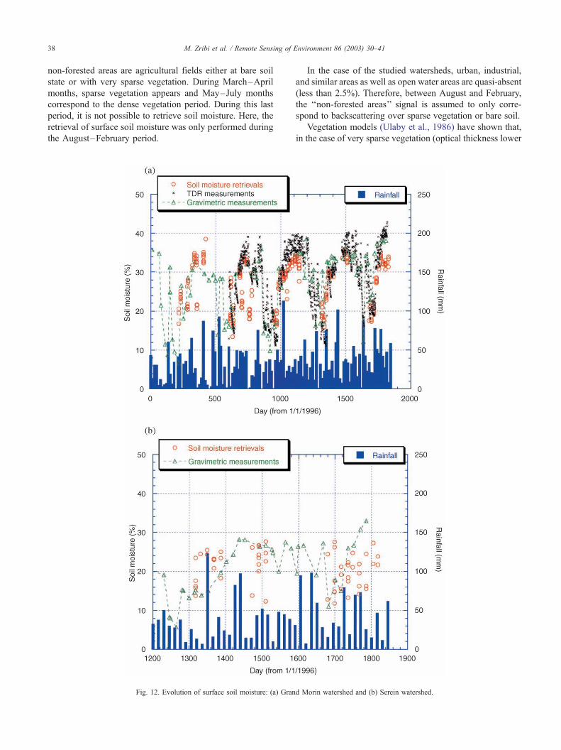
Fig. 12. Evolution of surface soil moisture: (a) Gran

In the case of the studied watersheds, urban, industrial,

and similar areas as well as open water areas are quasi-absent

(less than 2.5%). Therefore, between August and February,

the ‘‘non-forested areas’’ signal is assumed to only corre-

spond to backscattering over sparse vegetation or bare soil.

Vegetation models (Ulaby et al., 1986) have shown that,

in the case of very sparse vegetation (optical thickness lower

d Morin watershed and (b) Serein watershed.


than 0.1) and in a first approximation, the backscattering

signal at low incidence angles only depends on bare soil

features. Inversely to the contribution from vegetation,

which is fairly stable with the incidence angle, the bare soil

backscattering coefficient decreases rapidly with the inci-

dence angle. To ensure both that the considered signal is

principally dependent on soil moisture and not on vegetation

features, and a high dependence of the backscattering slope

function with the incidence angle, only the low incidence

angles are kept in the soil moisture inversion process. Then,

the WSC measurements at incidence angles lower than 30jwere kept and the methodology described in Section 3.2.2

was applied.

Fig. 11 shows the soil moisture retrievals in the cases of

the Grand Morin and the Petit Morin watersheds during

August–February periods and the 3 years studied (1996–

1998). Soil moisture estimations are compared with ground

truth data acquired by TDR measurements. Each watershed

is covered by different WSC cells (eight in the case of the

Grand Morin and four in the case of the Petit Morin). At a

given date, the plotted soil moisture estimations correspond

to the different estimations obtained on each of these cells.

The ground-truth TDR data are also represented on the

graph. Fig. 11 clearly shows the good performance of the

proposed method on the retrieval of soil moisture during

winter months. The correlation coefficients R2 are greater

than 0.8 and rms errors are lower than 3.5% for the two

watersheds. We also observe a bi-modal structure of our

database: high (>30%) and low soil moistures (around

20%). Since it could increase the computed correlation

coefficient (but does not affect the rms error), it may be

interesting to valid our approach also on some data sets

showing more uniformly distributed soil moistures.

Finally, Fig. 12 shows, for the 3-year time period and the

Grand-Morin and Serein watersheds, the time variation of

the soil moisture retrievals compared to ground truth meas-

urements. A small discrepancy (generally lower than 5%)

may be observed between volumetric soil moisture measure-

ments performed with TDR probes and gravimetric ones. It

is probably mainly due to the fact that TDR are very local

measurements whereas gravimetric ones are averaged over

the watershed, and/or to a small error in the estimation of the

bulk soil density. Fig. 12 shows that the annual cycle of soil

moisture is quite well retrieved by ERS data: high moisture

level for winter rainy period (November–February) and a

lower level for dry period (end of Summer). However, for

some dates (day 699 for example), a large difference

between measurements and estimations (about 10%) is

observed. This is probably due to WSC/ERS calibration,

since it is observed for all the tested cells. The data are also

compared to rainfall observations: high soil moistures are

associated to rainfall events, and the dry periods correspond

to a decrease in soil moisture. Unfortunately, the selection of

incidence angles lower than 30j limits the number of

measurements (approximately two measurements per month

remain).

For the Serein watershed, since no daily TDR measure-

ments are available, the comparison is done with the

gravimetric measurements for some dates. Consequently,

the conclusions for this site are only qualitative.

4. Conclusion

This paper presents a methodology to monitor soil

moisture at large scale over sparse vegetation or bare soils

areas, based on the synergistic use of the two active micro-

wave instruments of the ERS satellites (the wind scatter-

ometer and the SAR). The WSC signal is represented as the

incoherent sum of backscattered signals by different patches

of land uses. Over agricultural areas, the two main land uses,

which can be distinguished, are forests and agricultural

lands. The two contributions may be weighted by their

respective fractional cover. More specifically, for the period

of August–February, agricultural lands are mostly com-

posed of bare soils or sparse vegetation covers such as

wheat fields before raising, but not permanent grassland

areas which are generally too dense. Therefore, we consider

that the radar WSC signal is an incoherent sum of forest and

bare soil effects. Thanks to the high resolution SAR

imagery, the forest signal evolution can be retrieved for 2

years over the studied region. A cyclic behaviour is

observed, and the forest signal is modelled as a function

of time and incidence angle. The fraction of forest within

each WSC cell has been known from classification imagery

interpretation and the backscattered signal over bare soils

can be retrieved. IEM model is used to model the behaviour

of backscattering over bare soil. It is shown that the differ-

ence between radar simulations acquired simultaneously

with two different incidence angles are quasi-independent

of soil moisture. Therefore, we propose to use measure-

ments acquired with midbeam and forebeam antennae to

estimate roughness parameters. Then, soil moisture is

retrieved using a semi-empirical backscattering relationship

(linear approximation based on the IEM). Retrieved soil

moistures for different cell measurements over the studied

watersheds are compared with experimental data. They

show a good agreement with correlation coefficients R2

greater than 0.8 and root mean square errors lower than

3.5%. Among the restrictions, we must note that the method

described here is specifically developed for agricultural

regions principally composed of forests and cultivated areas.

Future studies are carried out to generalize this approach for

other regions concerned by other types of forests or a higher

percentage of grassland areas.

Acknowledgements

The authors would like to thank P.L. Frison for his help

concerning the processing of the WSC data. We also thank

CERSAT for providing us with the ERS scatterometer data.


Thanks to the European AIMWATER program, where the

SAR data as well as the soil moisture in situ measurements

have been acquired (no. ENV4-CT98-0740).

Appendix A

IEM (Fung et al., 1992) is based on analytical solutions

of the integral equations for tangential surface fields on a

dielectric interface. The model can be applied for different

types of soil surfaces. In IEM, the soil roughness is

characterised by two parameters: the root mean square

(rms) height, and the correlation length.

For the wave numbers, surface rms heights and surface

correlation lengths within the domain validity of the model

(small and moderate roughness surfaces), the backscattering

coefficient r0 can be written:

r0pp ¼

k2

2exp½�2k2z s

2Xln¼1

s2nAInppA2 W

ðnÞð�2kx; 0Þn!

; p ¼ h; v

ð16Þ

Where kz = k cos hi, kx = k sin hi, hi is the incident angle, k

the wave number, and s the rms height of surface. Ippn is a

function of the incidence angle, soil dielectric constant, s,

and the Fresnel reflection coefficient. W (n) (� 2kx,0) is the

Fourier transform of the nth power of the surface correlation

function.

This IEM version (Wu et al., 2001) introduces the transi-

tional function in which the Fresnel reflection coefficient

Rp(T) is not evaluated for an incidence angle hi, but for anangle ranging from hi to the normal incidence. It writes:

RpðTÞ ¼ RpðhiÞ þ tRpðhspÞ � RpðhiÞbcp; p ¼ h; v ð17Þ

where Rp (hi) is the Fresnel reflection coefficient calculated

at the incidence angle, Rp (hsp) is the Fresnel reflection

coefficient calculated at the specular angle and cp is a

transition function dependent on polarisation, incidence

angle, and surface parameters.

The IEM input parameters are the dielectric constant

derived from the surface volumetric moisture content and

the soil texture (Hallikanen, Ulaby, Dobson, El-Rayes, &

Wu, 1985), and the correlation function of surface heights,

or its corresponding spectrum. In the case of agricultural soil

studies, an exponential correlation function generally gives

a good fit with the majority of experimental surfaces.

References

Betts, A. K., Ball, J. H., Beljaars, A. C. M., Miller, M. J., & Viterbo, P. A.

(1996). The land surface-atmosphere interaction: a review based on

observational and global modeling perspectives. Journal of Geophysi-

cal Research, 101(D3), 7209–7225.

Beven, K. J., & Fisher, J. (1996). In J. B. Stewart, E. T. Engman, R. A.

Feddes, & Y. Kerr (Eds.), Remote sensing and scaling in hydrology,

scaling in hydrology using remote sensing. Chichester, England: John

Wiley & Sons.

Bezdek, J. C., Ehrlich, R., & Full, W. (1984). FCM: the fuzzy c-means

algorithm. Computer and Geoscience, 10(2–3), 191–203.

Boisvert, J. -B., Gwyn, Q. H. J., Chanzy, A., Major, D. -J., Brisco, B., &

Brown, R. -J. (1997). Effect of surface soil moisture gradients on mod-

eling radar backscattering from bare fields. International Journal of

Remote Sensing, 18(1), 153–170.

Cognard, A. -L., Loumagne, C., Normand, M., Olivier, P., Ottle, C., Vidal-

Madjar, D., Louahala, S., & Vidal, A. (1995). Evaluation of the ERS1/

Synthetic Aperture Radar capacity to estimate surface soil moisture: two

year results over the Naizin watershed. Water Resources Research, 31,

975–982.

De Roo, P. J., Offermans, R. J. E., & Cremers, N. H. (1996). LISEM: a

single-event, physically based hydrological and soil erosion model for

drainage basins. II: sensitivity analysis, validation and application. Hy-

drological Processes, 10, 1119–1126.

Dubois, P. C., Van Zyl, J., & Engman, T. (1995). Measuring soil moisture

with imaging radars. IEEE Transactions on Geoscience and Remote

Sensing, 33(4), 915–926.

Frison, P. L., & Mougin, E. (1996). Use of ERS-1 wind scatterometer data

over land surfaces. IEEE Transactions on Geoscience and Remote Sens-

ing, 34, 1–11.

Fung, A. K. (1994). Microwave scattering and emission models and their

applications. Norwood, MA: Artech House.

Fung, A. K., Li, Z., & Chen, K. S. (1992). Backscattering from a randomly

rough dielectric surface. IEEE Transactions on Geoscience and Remote

Sensing, 30(2), 356–369.

Giordano, A., et al. (1990). CORINE soil erosion risk and important land

resources. Publication of the European Communities, 13233, EN.

Hallikanen, M. T., Ulaby, F. T., Dobson, M. C., El-Rayes, M., & Wu, L.

(1985). Microwave dielectric behavior of wet soil—Part I: empirical

models and experimental observations. IEEE Transactions on Geosci-

ence and Remote Sensing, 23(1), 25–34.

Jackson, T. -J., Schmugge, J., & Engman, E. -T. (1996). Remote sensing

applications to hydrology: soil moisture. Hydrological Sciences, 41(4),

517–530.

Jarlan, L., Mougin, E., Frison, P. L., Mazzega, P., & Hiernaux, P. (2002).

Analysis of ERS wind scatterometer time series over Sahel (Mali).

Remote Sensing of Environment, 81, 404–415.

Kennett, O. G., & Li, F. K. (1989). Seasat over land scatterometer data. Part

I: global overview of the Ku-band backscatter coefficient. IEEE Trans-

actions on Geoscience and Remote Sensing, 27, 592–605.

Kerr, Y. H., Waldteufel, P., Wigneron, J. -P., Martinuzzi, J. M., Font, J., &

Berger, M. (2001). Soil moisture retrieval from space: the soil moisture

and ocean salinity (SMOS) mission. IEEE Transactions on Geoscience

and Remote Sensing, 39(8), 1729–1735.

Le Hegarat-Mascle, S., Quesney, A., Vidal-Madjar, D., Taconet, O., Nor-

mand, M., & Loumagne, C. (2000). Land cover discrimination from

multitemporal ERS images and multispectral LANDSAT images: a

study case in an agricultural area in France. International Journal of

Remote Sensing, 21, 435–456.

Le Hegarat-Mascle, S., Zribi, M., Alem, F., Weisse, A., & Loumagne, C.

(2002). Soil moisture estimation from ERS/SAR data: toward an opera-

tional methodology. IEEE Transactions on Geoscience and Remote

Sensing, 40(12), 1–12.

Magagi, R. D., & Kerr, Y. H. (1997). Retrieval of soil moisture and veg-

etation characteristics by use of ERS-1 wind scatterometer over arid and

semi-arid areas. Journal of Hydrology, 188–189, 361–384.

Magagi, R. D., & Kerr, Y. H. (2001). Estimating surface soil moisture and

soil roughness over semiarid areas from the use of the copolarization

ratio. Remote Sensing of Environment, 75(3), 432–445.

Ogilvy, O. (1991). Theory of wave scattering from random rough surfaces.

Bristol: Adam Hilger.

Oh, Y., Sarabandi, K., & Ulaby, F. T. (1992). An empirical model

and an inversion technique for radar scattering from bare soil


surfaces. IEEE Transactions on Geoscience and Remote Sensing, 30(2),

370–381.

Paloscia, S., Macelloni, G., Santi, E., & Koike, T. (2001). A multifrequency

algorithm for the retrieval of soil moisture on a large scale using micro-

wave data from SMMR and SMM/I satellite. IEEE Transactions on

Geoscience and Remote Sensing, 39(8), 1655–1666.

Prevot, L., Dechambre, M., Taconet, O., Vidal-Madjar, D., Normand, M.,

& Galle, S. (1993). Estimating the characteristics of vegetation canopies

with airborne radar measurements. International Journal of Remote

Sensing, 14(15), 2803–2818.

Prigent, C., Rossow, W. B., Matthews, E., Marticorena, B., 1999. Micro-

wave radiometric signatures of different surface types in deserts. Jour-

nal of Geophysical Research, 104(D10), 147–12, 158–12.

Quesney, A., Le Hegarat-Mascle, S., Taconet, O., Vidal-Madjar, D.,

Wigneron, J. P., Loumagne, C., & Normand, M. (2000). Estimation

of watershed soil moisture index from ERS/SAR data. Remote Sensing

of Environment, 72, 290–303.

Rakotoarivony, L., Taconet, O., Vidal-Madjar, D., & Benallegue, M.

(1996). Radar backscattering over agricultural bare soils. Journal of

Electromagnetic Waves and Applications, 10(2), 187–209.

Shi, J., Wang, J., Hsu, A. Y., O’Neill, P. E., & Engmann, T. (1997).

Estimation of bare surface soil moisture and surface roughness param-

eter using L-band SAR image data. IEEE Transactions on Geoscience

and Remote Sensing, 35(5), 1254–1265.

Ulaby, F. T., Aslam, A., & Dobson, M. C. (1982). Effects of vegetation

cover on the radar sensitivity to soil moisture. IEEE Transactions on


Ulaby, F. T., Moore, R. K., & Fung, A. K. (1986). Microwave remote

sensing active and passive. Norwood, MA: Artech House.

Wagner, W., Lemoine, G., Borgeaud, M., & Rott, H. (1999). A study of

vegetation cover effects on ERS Scatterometer data. IEEE Transactions

on Geoscience and Remote Sensing, 37(2), 938–948.

Wang, J., Hsu, A., Shi, J. C., O’Neil, P., & Engman, T. (1997). Estimating

surface soil moisture from SIR-C measurements over the Little Washita

River watershed. Remote Sensing of Environment, 59, 308–320.

Wegmuller, U., Matzler, C., & Schanda, E. (1989). Microwave signature of

bare soil. Advances in Space Research, 9(1), 307–316.

Woodhouse, I. H., & Hoekman, D. H. (2000). Determining land surface

parameters from the ERS-1 wind-scatterometer. IEEE Transactions on


Wu, T. D., Chen, K. S., Shi, J., & Fung, A. K. (2001). A transition model

for the reflection coefficient in surface scattering. IEEE Transactions on


Zribi, M., & Dechambre, M. (2002). A new empirical model to retrieve soil

moisture and roughness from C-band radar data. Remote Sensing of

Environment, 84, 42–52.

surface soil moisture estimation from the synergistic use...

Documents