surface finite element method for pattern formation on evolving

J. Math. Biol.DOI 10.1007/s00285-011-0401-0 Mathematical Biology

The surface finite element method for patternformation on evolving biological surfaces

R. Barreira · C. M. Elliott · A. Madzvamuse

Received: 5 May 2010 / Revised: 4 December 2010© Springer-Verlag 2011

Abstract In this article we propose models and a numerical method for patternformation on evolving curved surfaces. We formulate reaction-diffusion equations onevolving surfaces using the material transport formula, surface gradients and diffusiveconservation laws. The evolution of the surface is defined by a material surface veloc-ity. The numerical method is based on the evolving surface finite element method. Thekey idea is based on the approximation of � by a triangulated surface �h consistingof a union of triangles with vertices on �. A finite element space of functions is thendefined by taking the continuous functions on �h which are linear affine on each sim-plex of the polygonal surface. To demonstrate the capability, flexibility, versatility andgenerality of our methodology we present results for uniform isotropic growth as wellas anisotropic growth of the evolution surfaces and growth coupled to the solutionof the reaction-diffusion system. The surface finite element method provides a robustnumerical method for solving partial differential systems on continuously evolvingdomains and surfaces with numerous applications in developmental biology, tumourgrowth and cell movement and deformation.

R. BarreiraEscola Superior de Tecnologia do Barreiro/IPS, Rua Américo da Silva Marinho-Lavradio,2839-001 Barreiro, Portugale-mail: [email protected]

C. M. ElliottMathematics Institute and Centre for Scientific Computing, University of Warwick,Coventry CV4 7AL, UKe-mail: [email protected]

A. Madzvamuse (B)Department of Mathematics, University of Sussex, Falmer, Brighton, BN1 9QH, UKe-mail: [email protected]

123

R. Barreira et al.

Keywords Pattern formation · Evolving surfaces · Surface finiteelement method · Reaction-diffusion systems · Activator-depleted model

Mathematics Subject Classification (2000) 35K57 · 35K58 · 37C60 · 65M60 ·9108 · 9208

1 Introduction

The purpose of this paper is to formulate reaction-diffusion equations on evolvingsurfaces and to propose a novel numerical approach based on the surface finite ele-ment method. The context is that of pattern formation on a growing biological sur-face modelled by reaction-diffusion equations following the classical paper of Turing(1952). Such equations exhibit diffusion-driven instability of spatially uniform struc-tures leading to spatially non-uniform patterns. Many mathematical models basedupon this work were later developed and analysed motivated by applications such aspattern formation in hydra, sequential pattern formation in vertebrates, coat mark-ings of animals and pigmentation patterns on butterfly wings, amongst others. For anoverview we refer the reader to Murray (2002).

The original work of Turing did not take into account growth and changes in geom-etry. However, these factors are important in the development of patterns observed innature. Pattern formation on growing domains has been widely studied. For exampleCrampin et al. (1999) considers domain growth for a one-dimensional domain andshows that it may be a mechanism for increasing the robustness of pattern formationwith respect to the initial conditions. In the context of understanding the evolution of thestripes observed in the fish Pomacanthus (Kondo and Asai 1995), a two-dimensionalgrowing planar domain was considered in Maini et al. (1997). See also Madzvamuseet al. (2009) where the Turing diffusively-driven instability conditions are general-ised to reaction-diffusion systems with slow, isotropic domain growth. The numericalmethod proposed in this article is a tool to explore such reaction kinetics on evolvingsurfaces.

Much interesting work has been carried out for growing planar domains. How-ever in applications to biological forms it is natural to consider pattern formation onan evolving curved surface which is the boundary of a growing three-dimensionaldomain. For example we refer to Aragón et al. (1999) and Barrio et al. (2004) wherethe effects of curvature in the selection of patterns on a stationary sphere and growingcones were studied. Another initial study is the work in Chaplain et al. (2001) whichpresents a numerical method for the problem of pattern formation on spherical sur-faces with applications to solid tumour growth. Their numerical method is based onparameterising the surface over a sphere and then using the method of lines.

Our approach is based on the surface finite element method which is a naturalextension of the finite element method (Madzvamuse et al. 2003) and is capable ofhandling complex geometries and shapes (Dziuk and Elliott 2007a,b; Eilks and Elliott2008; Barrett et al. 2008; Barreira 2009; Elliott and Stinner 2010). The idea is to trian-gulate the surface and approximate the system of partial differential equations usingpiece-wise linear surface finite element spaces based on the triangulation. In this paperwe are interested in evolving surfaces. In this instance the vertices of the triangulation

123

The surface finite element method for pattern formation

are moved with a velocity which is either prescribed or is governed by some evolutionlaw. In order to do this we need to formulate an appropriate conservation law on thesurface. The evolving surface finite element method exploits the special features ofthis conservation law when written in an appropriate variational form.

The reaction-diffusion equations on evolving surfaces are formulated in Sect. 2.Within this framework we establish appropriate notation for surface gradients whichis key to deriving from first principles reaction-diffusion systems on evolving sur-faces. For illustrative purposes we consider the well-studied activator-depleted sub-strate model (Gierer and Meinhardt 1972; Prigogine et al. 1968; Schnakenberg 1979)also known as the Brusselator model as a reaction-kinetic candidate for exploration.Similarly, any other plausible reaction kinetics can be easily treated in this framework.We also discuss the formulation of models for surface growth.

In Sect. 3 we present the evolving surface finite element method applied to reac-tion-diffusion systems on evolving surfaces which change shape. A feature of thevariational formulation is that certain geometric quantities such as the mean curvatureand normal of the surface do not appear. This is then taken advantage of in a naturalway by the finite element method. In this approach no transformations or parameteri-sations are required in formulating either the reaction-diffusion system or the surfacefinite element method. Discretising in space results in a system of nonautonomousordinary differential equations which is discretised in time. In particular because thisapplication involves semilinear parabolic equations we linearise nonlinear kineticsfollowing Madzvamuse (2006) to obtain a linear algebraic system. This system is thensolved using the GMRes algorithm (Golub and Van Loan 1996).

In Sect. 4 we present Turing patterns on fixed and evolving surfaces. We demon-strate the general applicability of the surface finite element method which has thecapability of handling anisotropic growth that might result from biological models.Our results confirm that incorporating domain growth enhances the pattern selectionprocess. The methodology is also applicable to models which couple the surface evo-lution to the reaction-diffusion system on the surface. This is illustrated in Sect. 5 withan application to modelling growth of solid tumours. Some concluding remarks aremade in Sect. 6.

Examples of other articles which also consider the numerical solution of surfacepartial differential equations include (Greer et al. 2006; Calhoun and Helzel 2009;Dziuk and Elliott 2010; Lefevre and Mangin 2010; Elliott et al. 2010). The article(Deckelnick et al. 2005) is a review of differing approaches to the computation ofevolving surfaces.

1.1 Software package

The computations described here were carried-out in the framework of the finite ele-ment software package ALBERTA (Schmidt and Siebert 2005).

2 Derivation of the reaction-diffusion equations on an evolving surface

Because we are dealing with surface partial differential equations we need theconcepts of hypersurfaces and surface gradients. We establish the notation to

123

R. Barreira et al.

be used throughout the paper in the next section following the accounts inDeckelnick et al. (2005),Dziuk and Elliott (2007a,b) and the references therein. A fea-ture of this approach is the avoidance of the use of parameterisations and charts.

2.1 Surface gradients

A subset � ⊂ R3 is called a C2-hyper-surface if it can be locally represented as the

graph of a C2-function over an open subset of R2. For convenience we will assume

that � can be globally represented as the zero level set of a function d, that is, thereexists an open set U ⊂ R

3 and a function d ∈ C2(U) such that

U ∩ � = {x ∈ U : d(x) = 0} , and ∇d(x) �= 0, ∀ x ∈ U ∩ �.

The tangent space at x ∈ � is the linear subspace of R3 that is orthogonal to ∇d(x)

(and is independent of the particular choice of d). A C2-hyper-surface is called ori-entable if there exists a vector field ν ∈ C1(R3) such that ν(x) is orthogonal to thetangent space and |ν(x)| = 1 for all x ∈ �. The orientation of � is determined bychoosing the normal ν to be in the direction of increasing d and we define the unitnormal vector field by

ν(x) = ∇d(x)

|∇d(x)| .

One possible choice for d is the signed distance function to � and in that case|∇d(x)| = 1, ∀ x ∈ �.

We define the tangential gradient of a function η which is differentiable in an openneighbourhood of � by

∇�η(x) = ∇η(x) − ∇η(x) · ν(x)ν(x), x ∈ �,

where ∇ denotes the usual gradient in R3. Note that ∇�η has three components and

that although the definition relies on extending η off the surface, ∇�η depends onlyon the surface values of η. We will use the following notation

∇�η(x) = (D1η(x), D2η(x), D3η(x)

).

If η is twice differentiable in an open neighbourhood of �, then the Laplace-Beltramioperator is defined as the tangential divergence of the tangential gradient:

��η(x) = ∇� · ∇�η(x) =3∑

i=1

Di Diη(x).

2.2 Reaction-diffusion systems on evolving surfaces

Let �(t) be an evolving two-dimensional hypersurface in R3 bounding a time-

dependent domain �(t) with unit outward pointing normal ν. Let the velocity of

123


material points on �(t) be denoted by v := V ν + vT where ν is the unit outwardpointing normal to �(t), V is the normal velocity and vT is a velocity field tangentialto the surface and hence orthogonal to ν. We follow the derivation in Dziuk and Elliott(2007a, 2010).

Let u be a vector of scalar concentration fields {ui }mi=1. For each concentration we

have a mass conservation law which balances the rate of change of the concentrationin an evolving material region with the outward flux and a net reactive production ratefi (u). Let R(t) be an arbitrary material portion of �(t) where each point moves withthe material velocity. According to the mass balance conservation law,

d

dt

∫

R(t)

ui = −∫

∂R(t)

qi · μ +∫

R(t)

fi (u), (1)

where, for each component i , qi and fi (u) are, respectively, the surface flux throughthe boundary of R(t) and the net production rate within the surface. The componentsof q normal to � do not contribute to the flux so we can assume q is a tangent vector.Using integration by parts it follows that

∫

∂R(t)

q · ν =∫

R(t)

∇� · q +∫

R(t)

q · νH =∫

R(t)

∇� · q.

On the other hand, for the left-hand side of (1), we use the transport formula (cf. Dziukand Elliott 2007b)

d

dt

∫

R(t)

η =∫

R(t)

∂•η + η∇� · v

for any material region of the surface evolving with the material velocity v where

∂•η := ηt + v · ∇η (2)

denotes the material derivative. Again observe that although this definition uses stan-dard derivatives of η which may be obtained by using an extension of η off the surface,the material derivative only depends on values of η on the time dependent surface.

Combining the two equations results in

∫

R(t)

∂•ui + ui∇� · v + ∇� · qi =∫

R(t)

fi (u).

Since R(t) is arbitrary for all time t , we conclude that

∂•ui + ui∇� · v + ∇� · qi = fi (u), on �(t). (3)

For the constitutive law relating the flux to the concentrations, assuming no cross-diffusion between the chemical species, we set D to be a diffusivity tensor (a diagonal

123

R. Barreira et al.

matrix diffusion coefficients) and assume that the chemical species diffuse accordingto Fick’s law

qi = −Di j∇�u j , (4)

where Di j = diδi j , with δi j representing the usual Kronecker delta function. Then (3)becomes

∂•ui + ui∇� · v = ∇�(Di j∇�u j ) + fi (u), on �(t).

In vector form, the system of reaction-diffusion equations on an evolving surface �(t)takes the form

∂•u + u∇� · v = D��u + f (u), (5)

where D = diag(di ). This system is supplemented with zero-flux boundary condi-tions if the boundary of �(t) is non-empty and the initial conditions

u(·, 0) = u0(·) on �(0) (6)

where the components of u0(·) are prescribed positive bounded functions.

Remark 1 Equation (5) is similar to the model investigated in Madzvamuse et al.(2005) for the planar case if we replace derivatives by tangential derivatives. Note thatin the planar case there is no normal velocity and v = vT .

Remark 2 Note that this derivation of the equation is for an arbitrary velocity fieldv which could depend on the surface �(t) itself and the solutions of the reaction-diffusion system.

2.3 Illustrative models

– Reaction kinetics

For simplicity we focus in this paper on the development of patterns modelled bya two component system so that u = (u, w) where u and w are the concentrationsof two chemical specimens. There are numerous models each of which leads to aparticular form of the reaction terms f1 and f2 in (5). We refer to Maini et al. (1997)for a review of commonly used reaction kinetics and their motivation. For illustrativepurposes we consider the activator-depleted substrate model (Gierer and Meinhardt1972; Prigogine et al. 1968; Schnakenberg 1979) also known as the Brusselator modelgiven by

f (u) = ( f1, f2)T =

(γ (a − u + u2w), γ (b − u2w)

)T(7)

123


where γ, a and b are positive constants. Observe that there is a unique solution tof (u) = 0 given by

u = a + b , w = b/(a + b)2 (8)

which corresponds to a unique steady state of (5) on a stationary surface. For a givenmodel, there may be a set of parameters, whose values belong to the Turing space,for which the model on fixed domains exhibits spatial pattern formation due to diffu-sion-driven instability of spatially uniform structures. For example on fixed domains,Murray (2002), summarises necessary conditions on the parameters a, b and d basedon linear stability analysis for Turing diffusion-driven instability to occur for the caseof the activator-depleted model.

Domain growth increases the range of biological morphogen pairings which havethe potential to induce Turing patterning compared to a fixed domain (Madzvamuse2009). It is now possible to suggest and investigate, for example, activator-activatoror short-range inhibition, long-range activation as paradigms for biological patternformation on growing domains. More generally, there exists a larger family of reactionkinetics capable of generating diffusively-driven instability patterns in the presence ofdomain growth (Madzvamuse 2009). Such models can be easily incorporated underthe surface finite element formulation. In this paper we restrict our attention to (7).

– Surface growthWe focus on three growth models for the evolution of the surface.– Isotropic growth

Here we assume that each material point on the surface undergoes the sameprescribed dilation so that if X (t) denotes a material point on �(t) then

X (t) = ρ(t)X0 (9)

where the dilation factor ρ(t) is a positive growth function satisfying the prop-erty that ρ(0) = 1. Note that in general such a surface growth involves both anormal velocity and a tangential velocity. However in the case of a sphere wemay write

X (t) = ρ(t)R0ν (10)

where ν is an arbitrary vector on the unit sphere so that the material velocity is

v(X (t), t) = X = V ν, with V = R0ρ(t)

and ν is the unit normal to the evolving surface.– Anisotropic growth

Here we are interested in a prescribed velocity law associated with non-isotropic growth. As an illustrative example we consider the following sur-face: let φ(x, t) be the prescribed level set function

φ(x, t) = x21 + x2

2 + a(t)2G(x23/L(t)2) − a(t)2 (11)

123

R. Barreira et al.

and the surface �(t) be described by the zero level set of φ. Different surfacesmay be obtained by prescribing the non-negative shape functions G(·), a(·)and L(·) with G(0) = 0 and G(1) = 1.

• Tangential and normal motionFor the given surface, material points may move in the tangential as well asthe normal direction. We set the surface �(t) to comprise material points(X (t), Y (t), Z(t)) and parameterise in the following way: given Z(0) ∈[−L(0), L(0)] choose (X (0), Y (0)) to lie on the circle

X (0)2 + Y (0)2 = a(0)2(1 − G(Z(0)2/L(0)2))

and

Z(t) = Z(0)L(t)

L(0), X (t) = X (0)

a(t)

a(0)and Y (t) = Y (0)

a(t)

a(0)

(12)

so that

φ(X (t), Y (t), Z(t), t) = 0.

• Normal motionOn the other hand we may choose material points on the same surfacebut such that the velocity of material points, v(X (t), Y (t), Z(t)), is in thenormal direction

v(x, t) = V (x, t)ν(x, t), ν(x, t) = ∇φ(x, t)

|∇φ(x, t)| and V (x, t) = − φt (x, t)

|∇φ(x, t)| .

– Chemically-driven surface evolutionWe envisage that the complex mathematical models for pattern formation onevolving surfaces will couple the growth process to surface concentration of species(or chemical concentrations) leading to the law of the form

V = g(u, ν, H) (13)

for the normal velocity where H is the mean curvature of the surface. Here weuse the definition of mean curvature to be the sum of the two principle curva-tures (Deckelnick et al. 2005) and the convention that the mean curvature of asphere is positive when the normal is oriented outwards of the ball. Actually onecould consider more general laws in which other geometric quantities such as theLaplace–Beltrami operator acting on the mean curvature (Elliott and Stinner 2010).Equations such as (13) arise naturally when the surface is energetic (Deckelnicket al. 2005). In addition to (13) there may also be an equation for the tangentialvelocity. In this paper we focus on an example for which the motion is in the normaldirection only.

123


3 Surface finite element method

In this section we present the surface finite element method applied to reaction-diffu-sion systems on evolving surfaces.

3.1 Variational formulation

For an arbitrary i

∂•ui + ui∇� · v = di��ui + fi (u). (14)

Let ϕ(·, t) ∈ H1(�(t)) be a test function. Multiplying (14) by ϕ and integrating over�(t) leads to

∫

�(t)

fi (u)ϕ =∫

�(t)

∂•uiϕ + uiϕ∇� · v − di

∫

�(t)

ϕ��ui

=∫

�(t)

∂•uiϕ + uiϕ∇� · v + di

∫

�(t)

∇�ui · ∇�ϕ −∫

∂�(t)

ϕ∇�ui · μ.

(15)

The last term vanishes if ∂�(t) = ∅ or ∂�(t) �= ∅ but ϕ = 0 or ∇�ui · μ = 0 on∂�(t). Hence, assuming any of these conditions holds we have

∫

�(t)

fi (u)ϕ =∫

�(t)

∂•uiϕ + uiϕ∇� · v + di

∫

�(t)

∇�ui · ∇�ϕ

=∫

�(t)

∂•(uiϕ) − ui∂•ϕ + uiϕ∇� · v + di

∫

�(t)

∇�ui · ∇�ϕ

= d

dt

∫

�(t)

uiϕ −∫

�(t)

ui∂•ϕ + di

∫

�(t)

∇�ϕ · ∇�ui . (16)

The variational form seeks to find ui ∈ H1(�(t)) satisfying

d

dt

∫

�(t)

uiϕ −∫

�(t)

ui∂•ϕ + di

∫

�(t)

∇�ϕ · ∇�ui

=∫

�(t)

fi (u)ϕ, ∀ϕ ∈ H1(�(t)). (17)

123

R. Barreira et al.

3.2 Evolving surface finite element method

We approximate �(t) by �h(t), a triangulated surface whose vertices lie on �(t),i.e. �h(t) = Th(t) = ⋃

k Tk(t), where each Tk(t) is a triangle. The diameter of thelargest triangle in the initial surface is denoted by h. We choose the vertices of thetriangulation to evolve with the material velocity so that

X j (t) = v(X j (t), t) (18)

and it is easy to see that X j (t) lies on �(t) if v is the exact material velocity. Weassume �h(t) is smooth in time. For each t we define a finite element space

Sh(t) ={φ ∈ C0(�h(t)) : φ

∣∣∣Tk

is linear affine for each Tk ∈ Th(t)

}.

For each t ∈ [0, T ] we denote by{χ j (·, t)

}Nj=1 the moving nodal basis functions and

by X j (t), j = 1, . . . , N the nodes. These functions will satisfy

χ j (·, t) ∈ C0(�h(t)), χ j (Xi (t), t) = δi j , χ j (·, t)∣∣Tk

is linear affine,

and on Tk ∈ Th(t)

χ j∣∣e = λk, for each e ∈ Th(t)

where k = k(Tk, j) and (λ1, λ2, λ3) are the barycentric coordinates.On �h(t) we define the discrete material velocity

vh =N∑

j=1

X j (t)χ j (19)

and the discrete material derivative

∂•hφ = φt + vh · ∇φ. (20)

Proposition 1 (Transport property) On �h(t), for each j = 1, . . . , N,

∂•hχ j = 0

and for each φ = ∑Nj=1 γ j (t)χ j ∈ Sh(t) then ∂•

hφ = ∑Nj=1 γ j (t)χ j .

Proof See Dziuk and Elliott (2007a).

We seek approximations Ui (·, t) ∈ Sh(t) to ui , for i = 1, 2. Since{χ j (·, t)

}Nj=1 is

the basis of Sh(t) we know for each Ui (·, t) ∈ Sh(t) and each t ∈ [0, T ] that there

123


exist unique αi = {α1

i (t), . . . , αNi (t)

}satisfying

Ui (·, t) =N∑

j=1

αji (t)χ j (·, t).

Substituting Ui (·, t), �h(t) and φ ∈ Sh(t) for ui , �(t) and ϕ in (17) we obtain

d

dt

∫

�h(t)

N∑

j=1

αji,tχ jφ −

∫

�(t)

N∑

j=1

αji,tχ j∂

•hφ +

∫

�h(t)

N∑

j=1

αj1χ jφ∇�h · vh

+ di

∫

�h(t)

N∑

j=1

αji (t)∇�h χ j · ∇�h(t)φ =

∫

�h

f1φ, (21)

for all φ ∈ Sh(t) and taking φ = χk, k = 1, . . . , N and using the transport propertyof the basis functions we obtain

d

dt(M(t)αi ) + diS(t)αi = Fi (t) (22)

where M(t) is the evolving mass matrix

M(t) jk =∫

�h(t)

χ jχk,

S(t) is the evolving stiffness matrix

S(t) jk =∫

�h(t)

∇�h χ j · ∇�h χk

and Fi is the right hand side Fi j = ∫

�h(t)fi (U)χ j .

Remark 3 The simple form of the system (22) is a consequence of the evolution oftriangle vertices by the material velocity (18). This is a Lagrangian discretisation.

3.3 Time discretization

For simplicity we restrict the description to the two component system u = (u, w)

with kinetics given by (7) and d1 = 1, d2 = d. We discretise in time using a uniformtime step τ . We represent by (U n, W n) the solution at time nτ and �n = �(nτ). Let

123

R. Barreira et al.

U 0, W 0 ∈ Sh(0) be given. For n = 0, . . . , nT , solve the nonlinear system

⎧⎪⎪⎪⎪⎪⎪⎪⎪⎪⎪⎪⎪⎪⎨

⎪⎪⎪⎪⎪⎪⎪⎪⎪⎪⎪⎪⎪⎩

1τ

∫

�n+1h

U n+1χn+1j + ∫

�n+1h

∇�nhU n+1 · ∇�n

hχn+1

j

= 1τ

∫

�nU nχn

j + ∫

�n+1h

f1(U n+1, W n+1

)χn+1

j ,

1τ

∫

�n+1h

W n+1χn+1j + d

∫

�n+1h

∇�nhW n+1 · ∇�n

hχn+1

j

= 1τ

∫

�nW nχn

j + ∫

�n+1h

f2(U n+1, W n+1

)χn+1

j ,

(23)

for all j = 1, . . . , N . To linearise f1(U n+1, W n+1

)we assume slow deformation

of the evolving surface which allows us to write(U n+1

)2 ≈ U nU n+1 (Madzvamuse2006).

Using this linearisation, we can derive the following fully discrete algorithm:

Let U0, W 0 ∈ Sh(0) be given. For n = 0, . . . , nT solve the linear system

⎧⎪⎪⎪⎪⎪⎪⎪⎪⎪⎪⎪⎪⎪⎪⎪⎨

⎪⎪⎪⎪⎪⎪⎪⎪⎪⎪⎪⎪⎪⎪⎪⎩

(1τ + γ

) ∫

�n+1h

Un+1χn+1j + ∫

�n+1h

∇�nh

Un+1 · ∇�nhχn+1

j

−γ∫

�n+1h

Un W nUn+1χn+1j = 1

τ

∫

�nUnχn

j + γ a∫

�nh

χnj ,

1τ

∫

�n+1h

W n+1χn+1j + d

∫

�n+1h

∇�nh

W n+1 · ∇�nhχn+1

j

+γ∫

�n+1h

(Un+1

)2W n+1χn+1

j = 1τ

∫

�nW nχn

j + γ b∫

�nh

χnj ,

(24)

for all j = 1, . . . , N . Using a matrix representation we have,

⎧⎪⎪⎨

⎪⎪⎩

((1τ + γ

)Mn+1 + Sn+1 − γMn+1

1

)Un+1 = 1

τ MnUn + Fn1 ,

(1τ Mn+1 + dSn+1 + γMn+1

2

)Wn+1 = 1

τ Mn Wn + Fn2 ,

(25)

with

Mni j =

∫

�nh

χni χn

j , Mn1 i j =

∫

�nh

Un W nχni χn

j , Mn2 i j =

∫

�nh

(Un+1

)2χn

i χnj ,

(26)Sn

i j =∫

�nh

∇�nhχn

i · ∇�nhχn

j , Fn1 i = γ a

∫

�nh

χni , Fn

2 i = γ b∫

�nh

χni ,

where χni ∈ Sn

h ={χ ∈ C0 (�h(nτ)) : χ j

∣∣e is linear affine for each e ∈ Th(nτ)

}.

123


Remark 4 The method requires a triangulation of the initial surface. For example, thesphere is triangulated in the following way. A very coarse triangulation is obtainedby hand using 6 points placed uniformly on the sphere. This triangulation is thensuccessively refined uniformly by subdividing each triangle into two. New verticesare then projected onto the surface of the sphere. This process is implemented inALBERTA which requires an algorithm for the projection of a point onto the surfacewhich is readily available for a sphere. This refinement is repeated until an acceptablemaximum mesh size is obtained.

Remark 5 We observe that various convergence results and error bounds have beenproved for the surface finite element. See Dziuk (1988); Dziuk and Elliott (2007a,b,2010) and the references cited therein.

4 Turing patterns

4.1 Turing patterns on fixed surfaces

As mentioned earlier we focus on the kinetics (7) with d1 = 1 and d2 = d. We begin bydescribing some simulations on a fixed surface. We choose the surface to be a sphereand fix the parameters a, b and d whilst varying γ . We also investigate the effect ofrefining the mesh for one of the examples.

4.1.1 The effect of varying γ

We use the following parameters: for the kinetics a = 0.1, b = 0.9 and for the dif-fusion coefficient, d = 10. Initial conditions are taken as small random perturbationsaround the homogeneous state (1, 0.9) which is a steady state for a stationary sur-face. Notice that this choice of parameter values satisfy the conditions necessary fordiffusion-driven instability on a fixed surface. Hence, we use the same parameters as(Madzvamuse 2006) on a static unit sphere in three simulations in which we vary onlyγ (see Table 1) in order to observe its effect on patterning. We point out that the initialconditions used were exactly the same for the three experiments. The results for theconcentrations u and w at t = 10 are displayed in Fig. 1. The colours red and orangerepresent high values in concentration while blue represents lower values.

As we can see in Fig. 1, the effect of varying γ while keeping all other parametersfixed is that the complexity of the pattern increases as γ increases. It must be noted thatγ represents the scale length, increasing γ is equivalent to increasing surface size. The

Table 1 Parameters used tosimulate reaction-diffusionEq. (5) on the unit sphere

Experiment d γ a b h Timestep End time

1 10 30 0.1 0.9 0.055 0.001 10

2 10 200 0.1 0.9 0.055 0.001 10

3 10 500 0.1 0.9 0.055 0.001 10

123

R. Barreira et al.

Fig. 1 Colour version online: concentration values u and w on a unit sphere at t = 10 for the choicesa = 0.1, b = 0.9, d = 10 and γ = 30, 200, 500. Red and orange colours represent high values inconcentration while blue represent lower values

same effect was observed in the numerical computations presented in Madzvamuseand Maini (2007) and Chaplain et al. (2001) for example, although in this last one theparameter values for a, b and d are different from the ones used in our work. Noticethat regions with high values of u correspond to low values of w and vice versa, i.e.the solution profiles of u and w are in opposite phase. From now onward we showonly solutions profiles corresponding to the concentration u.

4.1.2 The effect of mesh refinement

Here we demonstrate that the discretisation is accurate and robust by simulating theabove example with γ = 200 using different triangulations. An initial triangulation ofthe sphere with h ≈ 0.055 is uniformly refined twice by reducing the mesh size by afactor of 2. The time step is also refined by a factor of 2. All other parameter values areheld constant. The initial concentration is generated by a random perturbation aroundthe uniform steady state. Thus in order to compare solutions the simulations for thetwo refined meshes use an interpolation of the solution for the initial coarse mesh att = 0.1. In Table 2 we present the parameters used for each simulation. We observein Fig. 2 that the patterns are robust and quantitatively similar as h is varied. Also inFig. 3 we display the evolution of the maximum and minimum values that the discretesolution u attains on the sphere as a function of time for each simulation. The graphsindicate convergence as the mesh sizes decrease.

123


Table 2 Parameters used fornumerically solving thereaction-diffusion system (5) ona unit sphere using threedifferent triangulations

h Elements γ a b Timestep

0.0723 16384 200 0.1 0.9 2 × 10−3

0.0550 32768 200 0.1 0.9 1 × 10−3

0.0362 65536 200 0.1 0.9 5 × 10−4

Fig. 2 Colour version online: concentration values u obtained at t = 10 using three different triangulationsas shown in Table 2

4.2 Turing patterns on evolving surfaces

To demonstrate the applicability, flexibility, versatility and generality of our ESFEMwe illustrate in this section two different scenarios describing surface evolution. Thefirst example is that of an evolving sphere which grows at a logistic rate; that is theradius of the sphere grows exponentially in the initial stages and then saturates to alimiting finite fixed value at later stages of growth. This growth profile is plausiblefrom the biological perspective since all organisms grow to a finite fixed size duringthe later stages of growth. Other types of isotropic growth profiles such as exponentialor linear can be easily treated in this framework. Our second example demonstratesthe generality of our method by dealing with non-isotropic growth.

123

R. Barreira et al.

Fig. 3 Colour version online: evolution of minimum and maximum values of u for each of the threetriangulations. M1 is the coarser mesh (16384 elements), M3 is the most refined one (65536 elements)

4.2.1 Example 1: Logistic growth

For illustrative purposes we consider an evolving sphere given by (10) with initial unitradius. The sphere evolves according to the logistic growth function ρ(t) defined by

ρ(t) = ert

1 + 1K (ert − 1)

, (27)

where r > 0 and K > 1. Here r is the growth rate of the surface and K is the limitingfinal fixed size of the radius.

Figure 4 illustrates transient numerical solutions corresponding to the u concen-tration on an evolving sphere whose growth is defined by (27). Initial conditions aretaken as small random perturbations around the uniform steady state (1.0, 0.9). Snap-shot transient solutions are captured at times t = 10, 30 and 50 where the sphere

Fig. 4 Colour version online: numerical results illustrating the transient solutions corresponding to theu concentration on a continuously evolving sphere defined by (10). The sphere evolves according to thelogistic growth function (27). Model and numerical parameter values are given in Table 3

123


Table 3 Parameters used forreaction-diffusion simulation ona surface growing according tologistic growth

d γ a b K r Timestep Solver Solver Tol.

10 200 0.1 0.9 1.5 0.1 5 × 10−4 GMRes 10−9

is continuously evolving. At time t = 50, surface evolution is switched-off and thesolutions are allowed to evolve to an inhomogeneous steady state on the final staticsphere. The solution at time t = 70 appears to be a re-orientation (through rotation)of the transient solution at time t = 50.

We now consider the model equations on a static sphere whose radius is obtainedfrom the logistic growth function at time t = 50. For this numerical experiment, initialconditions at time t = 0 are taken as small random perturbations around the uniformsteady state as above. In Fig. 5 we illustrate the evolution of the inhomogeneous steadystate in the absence of surface evolution. A detailed bifurcation analysis on evolvingsurfaces is warranted in order to understand the differences between the patterns inFig. 4d and Fig. 5d and this is the subject of current studies.

4.2.2 Example 2: Anisotropic growth

Figure 6 illustrates the results of the implementation of the ESFEM applied to thereaction-diffusion system (5) where the surface �(t) is given by (11) and (12) withthe shape functions being

⎧⎨

⎩

L(t) = L0β+(1−β)e−r t ,

a(t) = a0(1 + α(1 − e−kt )

),

G(s) = s2p,

(28)

where L0 = 0.5, a0 = 0.1, α = 0.8, β = 0.3, r = 0.5, k = 0.5 and p = 5. The restof the parameters are listed in Table 4. Initial conditions are prescribed to be smallrandom perturbations around the uniform steady state obtained on a fixed surface.

We use a triangulation of the initial surface with 32700 elements and such that thelargest triangle diameter is h ≈ 0.0215. The initial triangulation was obtained using aC package Gnu triangulated surfaces (GTS) (http://gts.sourceforge.net/).

Fig. 5 Colour version online: numerical results illustrating the spatially inhomogeneous solutions corre-sponding to the u concentration on a static sphere of radius approximately 1.5 (the limiting radius of thelogistic growth function). Model and numerical parameter values are given in Table 3

123

http://gts.sourceforge.net/

R. Barreira et al.

Fig. 6 Colour version online:numerical transient solutionscorresponding to the uconcentration values at timest = 0, 0.1, 1.6, 1.64, 1.68 and2.75 on a surface evolvingaccording to anisotropic growthdefined by equations (11) and(28)

Table 4 Parameters used forreaction-diffusion simulation onan evolving surface (anisotropicgrowth)

d γ a b Timestep Solver Solver Tol.

100 500 0.1 0.9 5 × 10−4 GMRes 10−9

Fig. 7 Colour version online: detail of the mesh surrounding a breaking spot (at t = 1.64) for the patternformation on a surface evolving according to anisotropic growth

Figure 6 illustrates the results of our simulation with model parameter values inTable 4. Initially no patterns are observed, then spot-period doubling bifurcation startsto emerge with further evolution of the surface. Period doubling in spots occurs throughpeak splitting, a process studied in Crampin et al. (2002). Furthermore, similar bifurca-tion sequences were observed on two-dimensional growing domains with exponentialgrowth, see Madzvamuse and Maini (2007). In Fig. 7 detail of the mesh surrounding

123


a breaking spot is shown. It is clear that there is enough refinement to resolve theinterface between higher and lower concentration regions.

5 Pre-pattern theory applied to the growth of solid tumours

In this section we illustrate the application of ESFEM to a system coupling surfaceevolution with surface reaction-diffusion by considering a model for tumour growth.It is not our purpose to go deep into the biological motivation for the model of tumourgrowth or give an extensive background. We refer to Chaplain et al. (2001) for anoverview and provide just a brief description. We begin with a description of themodel, followed by a description of the numerical approach and finally present somenumerical simulations.

5.1 Model formulation

The model comprises the reaction-diffusion system (5) with activator-depleted kineticsof the form (7) and surface growth law of the form (13). Here u denotes the growth-promoting factor and w denotes the growth-inhibiting factor (Crampin et al. 1999).Furthermore, we consider the surface evolution to be governed by the normal velocityof the form

V = δu − εH (29)

where δ is a growth rate and ε may be considered to be a parameter which models thesurface tension of the tumour surface. We may also view ε as a small mathematicalparameter which regularises the evolution law. This is useful because it is easy tosee that even in the simple case of the surface velocity being constant in the normaldirection it is possible for smooth surfaces to develop corners in a short time.

Note that (29) is an equation for forced mean curvature flow of a surface (Dziukand Elliott 2010). In the paper (Chaplain et al. 2001) numerical simulations of thereaction-diffusion system were carried-out on a stationary sphere in a pre-patterningstage and then the solution was used to show how the surface might grow initiallyin preferred directions with a model such as (29) for ε = 0. The numerical methodof Chaplain et al. (2001) applied was based on the method of lines with sphericalharmonics. An advantage of ESFEM is that we only need the positions of the trianglevertices in order to compute, resulting in an attractive flexibility of the method.

5.2 Numerical method

The numerical algorithm consists of two steps: given �nh , Xn, Un

h ∈ Snh find Xn+1 and

Un+1h by solving:

123

R. Barreira et al.

1.

(1

τMn + εSn

)Xn+1 = 1

τMXn + Gn, (30)

where Xn denotes the nodal coordinates at time n and Mn and Sn are blockmass and stiffness matrices whose blocks are determined by the mass and stiff-ness matrices for the triangulated surface �n

h , respectively, and

Gni =

∫

�n

δ(Unh )1ν

nχi . (31)

Here the normal νn is computed separately for each face of the triangle.2. The newly computed coordinates of the triangle vertices Xn+1 are used to calcu-

late the mass and stiffness matrices at time level n +1. Then the following system

Table 5 Parameters used in thesimulation of tumour growth

d γ a b t δ ε Timestep Solver Solver Tol.

10 30 0.1 0.9 5. 0.1 0.01 0.001 GMRes 10−9

Fig. 8 Colour version online: concentration of the growth factor u for the tumour model with γ = 30

123


Fig. 9 Colour version online:initial and final triangulation forthe example of tumour modelwith (γ = 30)

(recalling (25)) is solved:

⎧⎨

⎩

(( 1τ

+ γ)Mn+1 + Sn+1 − γMn+1

1

)Un+1 = 1

τMnUn + Fn

1 ,(

1τMn+1 + dSn+1 + γMn+1

2

)Wn+1 = 1

τMn Wn + Fn

2 .(32)

5.3 Numerical results

The parameter values have been chosen to illustrate the effectiveness of ESFEM inhandling a problem for which the evolution of the surface depends on the solutionof the surface reaction-diffusion system. Initial conditions are prescribed as smallrandom perturbations around the homogeneous state (u(·, 0), w(·, 0)) = (1.0, 0.9).The initial surface is the unit sphere and this is approximated using a triangulation

123

R. Barreira et al.

Fig. 10 Colour version online: concentration of the growth factor u for the tumour model with γ = 200

with 32768 elements for which h ≈ 0.055. The rest of the parameters are given inTable 5.

In Fig. 8 we show a few snap-shots of the simulation of tumour growth by showingat the indicated times the tumour surface patterned by the concentration of the growthfactor u. As expected we observe that regions of higher values of u correspond toregions of higher growth evolution of the surface.

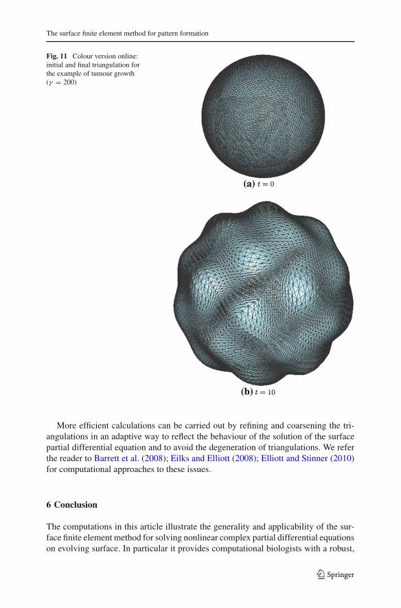
More complex structures for the tumour surface are obtained by increasing thevalue of γ . This is a consequence of the increase in complexity of the patterns of u onthe surface. Results are presented in Fig. 10 where all the parameters are the same as inTable 5 apart from the change of γ from 30 to 200. The initial and final triangulationsare displayed in Fig. 11.

5.3.1 Mesh adaptivity and remeshing

In principle after some time, since the vertices of triangles evolve according to thevelocity law, it is possible that triangulations of evolving surfaces may not be appro-priate for the simulation. For example they could degenerate in the sense of the appear-ance of very small angles. On the other hand the triangulation may not resolve thefeatures of the solution in subdomains where the concentrations change rapidly. Itis also possible that the topology of the surface could change as a consequence ofpinching-off and self-intersection. In the simulations presented in this paper a suit-ably uniformly refined initial triangulation was sufficient for the calculations. As canbe seen from the depicted final triangulations the evolving surfaces were adequatelyapproximated.

123


Fig. 11 Colour version online:initial and final triangulation forthe example of tumour growth(γ = 200)

More efficient calculations can be carried out by refining and coarsening the tri-angulations in an adaptive way to reflect the behaviour of the solution of the surfacepartial differential equation and to avoid the degeneration of triangulations. We referthe reader to Barrett et al. (2008); Eilks and Elliott (2008); Elliott and Stinner (2010)for computational approaches to these issues.

6 Conclusion

The computations in this article illustrate the generality and applicability of the sur-face finite element method for solving nonlinear complex partial differential equationson evolving surface. In particular it provides computational biologists with a robust,

123

R. Barreira et al.

stable, accurate and a highly flexible method to model arbitrary surface evolution.Future developments should include:

– Adaptivity and remeshing.– Application to complex models.– Development of methods for surface topology change.– Systematic study of particular systems.– Linkage to solutions of equations holding in bulk domains.– Bifurcation analysis on evolving surfaces.

Acknowledgments Part of RB’s research was carried out at the Department of Mathematics of the Uni-versity of Sussex supported by a Graduate Teaching Assistantship. RB has also used the computationalresources of the Center for Mathematics and Fundamental Applications of the University of Lisbon. AMwould like to acknowledge grant financial support from the LMS (R4P2), EPSRC (EP/H020349/1), theRoyal Society Travel grant (R4K1) and the Royal Society Research Grant (R4N9). The research of CMEhas been supported by the UK Engineering and Physical Sciences Research Council (EPSRC), GrantEP/G010404.

References

Aragón JL, Barrio RA, Varea C (1999) Turing patterns on a sphere. Phys Rev E 60:4588–4592Barreira R (2009) Numerical solution of non-linear partial differential equations on triangulated surfaces,

D.Phil Thesis, University of SussexBarrett JW, Garcke H, Nürnberg (2008) Parametric approximation of Willmore flow and related geometric

evolution equations. SIAM J Sci Comput 31:225–253Barrio RA, Maini PK, Padilla P, Plaza RG, Sánchez-Garduno F (2004) The effect of growth and curvature

on pattern formation. J Dyn Diff Equ 4:1093–1121Calhoun DA, Helzel C (2009) A finite volume method for solving parabolic equations on logically cartesian

curved surface meshes. SIAM J Sci Comput 6:4066–4099Chaplain MAJ, Ganesh M, Graham IG (2001) Spatio-temporal pattern formation on spherical surfaces:

numerical simulation and application to solid tumour growth. J Math Biol 42:387–423Crampin EJ, Gaffney EA, Maini PK (2002) Mode doubling and tripling in reation-diffusion patterns on

growing domains: a piecewise linear model. J Math Biol 44:107–128Crampin EJ, Gaffney EA, Maini PK (1999) Reaction and diffusion on growing domains: scenarios for

robust pattern formation. Bull Math Biol 61:1093–1120Deckelnick KP, Dziuk G, Elliott CM (2005) Computation of Geometric PDEs and Mean Curvature Flow.

Acta Numerica 14:139–232Dziuk G (1988) Finite Elements for the Beltrami operator on arbitrary surfaces. Lecture Notes in

Mathematics, Partial differential equations and calculus of variations, vol 1357. Springer, Berlin,pp 142–155

Dziuk G, Elliott CM (2007) Finite elements on evolving surfaces. IMA J Num Anal 27:262–292Dziuk G, Elliott CM (2007) Surface finite elements for parabolic equations. J Comp Math 25:430–439Dziuk G, Elliott CM (2010) An Eulerian approach to transport and diffusion on evolving surfaces. Comput

Vis Sci 13:17–28Dziuk G, Elliott CM (2010) L2 estimates for the evolving surface finite element method. Math Comp

(submitted)Eilks C, Elliott CM (2008) Numerical simulation of dealloying by surface dissolution via the evolving

surface finite element method. J Comp Phys 227:9727–9741Elliott CM, Stinner B (2010) Modeling and computation of two phase geometric biomembranes using

surface finite elements. J Comp Phys 229:6585–6612Elliott CM, Stinner B, Styles VM (2010) Numerical computation of advection and diffusion on evolv-

ing diffuse interfaces. IMA J Num Anal. Advance Access published on 11 May 2010. doi:10.1093/imanum/drq005

Gierer A, Meinhardt H (1972) A theory of biological pattern formation. Kybernetik 12:30–39Golub GH, Van Loan CF (1996) Matrix Computations. JHU Press, Baltimore

123

http://dx.doi.org/10.1093/imanum/drq005

http://dx.doi.org/10.1093/imanum/drq005


Greer J, Bertozzi AL, Sapiro G (2006) Fourth order partial differential equations on general geometries.J Comput Phys 216:216–246

Kondo S, Asai R (1995) A reaction-diffusion wave on the skin of the marine anglefish, Pomacanthus. Nature376:765–768

Lefevre J, Mangin J-F (2010) A reaction-diffusion model of the human brain development. PLoS ComputBiol 6:e1000749

Madzvamuse A, Maini PK, Wathen AJ (2003) A moving grid finite element method applied to a modelbiological pattern generator. J Comp Phys 190:478–500

Madzvamuse A, Wathen AJ, Maini PK (2005) A moving grid finite element method for the simulation ofpattern generation by Turing models on growing domains. J Sci Comp 24(2):247–262

Madzvamuse A (2006) Time-stepping schemes for moving grid finite elements applied to reaction-diffusionsystems on fixed and growing domains. J Comput Phys 216:239–263

Madzvamuse A, Maini P (2007) Velocity-induced numerical solutions of reaction-diffusion systems oncontinuously growing domains. J Comput Phys 225:100–119

Madzvamuse A (2009) Turing instability conditions for growing domains with divergence free mesh veloc-ity. Nonlinear Anal Theory Methods Appl 12:2250–2257

Madzvamuse A, Gaffney EA, Maini PK (2009) Stability analysis of non-autonomous reaction-diffusionsystems: the effects of growing domains. J Math Biol 61:133–164

Maini PK, Painter KJ, Chau HNP (1997) Spatial pattern formation in chemical and biological systems.Faraday Trans 93:3601–3610

Murray JD (2002) Mathematical biology I and II, 3rd edn. Springer, BerlinPlaza RG, Sánchez-Garduño F, Padilla P, Barrio RA, Maini PK (2004) The effect of growth and curvature

on pattern formation. J Dynam Diff Eqs 16(4):1093–11214Prigogine I, Lefever R (1968) Symmetry breaking instabilities in dissipative systems. II. J Chem Phys

48:1695–1700Schnakenberg J (1979) Simple chemical reaction systems with limit cycle behaviour. J Theor Biol 81:389–

400Schmidt A, Siebert KG (2005) Design of adaptive finite element software: the finite element toolbox

ALBERTA, vol 42. Lecture notes in computational science and engineering. Springer, BerlinTuring A (1952) The chemical basis of morphogenesis. Phil Trans R Soc Lond B 237:37–72

123

surface finite element method for pattern formation on evolving

Documents