surface charges, holographic renormalization, and lifshitz spacetime … · surface charges,...

Surface Charges, Holographic Renormalization,

and Lifshitz Spacetime

Kristian Holsheimer

M.Sc. Thesis

Abstract

Two distinct holographic methods are introduced and applied in order to study field the-ories with a quadratic dispersion at strong coupling. The first holographic method is theone introduced by Brown & Henneaux almost 25 years ago, in which the Virasoro algebrais derived from purely classical Einstein gravity. The second method is the holographicrenormalization group in the Hamilton–Jacobi canonical formalism, which spawned fromthe AdS/CFT correspondence. Several fun examples of these methods are used to get a feelfor them, which include Strominger’s consistency check relating the Bekenstein–Hawkingentropy to the Cardy formula of the BTZ black hole. Both methods are finally applied tothe study of Lifshitz spacetime, which is a spacetime that has anisotropic scale invariance.The anisotropy is closely related to deviations from a linear dispersion; this thesis focuseson the case of quadratic dispersion E ∼ p2.

Although most techniques that are discussed emanated from string theory, they seem tobe valid alongside any consistent quantum theory of gravity. Basic knowledge of quantumfield theory, general relativity, group theory, and conformal field theory is presumed.

Under supervision of:

Prof. Jan de Boer

Instituut voor Theoretische FysicaUniversiteit van AmsterdamThe Netherlands

Prof. Alexander Maloney

McGill UniversityPhysics DepartmentMontreal QC, Canada

Enjoy!

Contents

Introduction 7

1 Surface Charges in AdS3 9

1.1 Metrics and Global Symmetries of AdS3 . . . . . . . . . . . . . . . . . . . 11

1.2 Asymptotic Symmetries and Surface Charges . . . . . . . . . . . . . . . . . 16

1.3 Brown–Henneaux 1986 . . . . . . . . . . . . . . . . . . . . . . . . . . . . . 20

1.4 Strominger’s Application of Cardy’s Formula . . . . . . . . . . . . . . . . . 24

2 Holographic Renormalization in Hamilton–Jacobi Formalism 29

2.1 Hamilton–Jacobi Formulation of Gravity . . . . . . . . . . . . . . . . . . . 31

2.2 Expanding The Hamilton Constraint . . . . . . . . . . . . . . . . . . . . . 34

2.3 From Radial to RG Flow . . . . . . . . . . . . . . . . . . . . . . . . . . . . 39

3 Lifshitz/Schrodinger Asymptotics 43

3.1 Lifshitz Spacetime with Schrodinger Symmetry . . . . . . . . . . . . . . . . 45

3.2 Holographic Renormalization of Lifshitz . . . . . . . . . . . . . . . . . . . 49

Appendix 55

A Killing–Cartan Metrics . . . . . . . . . . . . . . . . . . . . . . . . . . . . . 55

B Hamilton–Jacobi Formalism . . . . . . . . . . . . . . . . . . . . . . . . . . 57

C Gauss–Codazzi Equations . . . . . . . . . . . . . . . . . . . . . . . . . . . 60

D Temporal and Radial Gravitational Hamiltonian . . . . . . . . . . . . . . . 65

E Hamilton–Jacobi surface charges. . . . . . . . . . . . . . . . . . . . . . . . 74

F Code For Computing Surface Charges . . . . . . . . . . . . . . . . . . . . . 78

Index 84

Bibliography 86

Samenvatting Non-Technical Summary in Dutch 91

Acknowledgements

I would like to thank my advisors Jan de Boer and Alex Maloney, and the nice people atMcGill for the warm welcome. I especially thank Kyriakos Papadodimas, Balt van Rees,and Omid Saremi for answering virtually any physics related question that popped in myhead. I also thank Marco Baggio for many useful discussions. Finally, I would like to thankmy family for being so supportive.

Cheers!

Introduction

AdS/CFT correspondence. Gauge/gravity dualities such as the celebrated anti-DeSitter/conformal field theory correspondence [1–3] are concrete realizations of ’t Hooft andSusskind’s holographic principle [4]. Maldacena’s AdS/CFT conjecture [1] states that thereis an exact equivalence between string theory on an AdS background and a conformallyinvariant quantum field theory on the conformal boundary of AdS. This correspondence isholographic in nature, as it relates a theory in d+1 dimensions to a theory in d dimensions.In order to make the correspondence more tangible, one can take suitable limits such thatthe string-theory side is well approximated by ordinary (super)gravity, i.e. such that itis weakly coupled. The AdS/CFT correspondence relates the weakly-coupled regime onone side to the strongly-coupled regime on the other, so the corresponding boundary fieldtheory in the ‘suitable limits’ is necessarily strongly coupled.i

Holographic renormalization. It turns out that the radial coordinate on the gravityside is closely related to the renormalization group scale in the boundary theory. Thisrealization has spawned an interesting field of study known as holographic renormalization,cf. [7, 8]. The main idea in holographic renormalization is to find renormalized correlationfunctions in the strongly-coupled boundary QFT by doing computations on the gravityside of the correspondence. Namely, the QFT correlation functions typically have UVdivergences, which are translated to IR (large radius r) divergences on the gravity side.The name of the game is then to remove these large-r divergences, hence to renormalizethe QFT correlators holographically.

Anisotropic scaling. Apart from the well-known AdS/CFT correspondence, there hasbeen a lot of interest in studying field theories by building phenomenological models bymeans of gravity duals. Such studies go by the name AdS/QCD or AdS/condensed matter(for obvious reasons). In this thesis we will discuss a phenomenological gravity dual toa generic field theory at a Lifshitz-like fixed point. Instead of the usual scale-invariancexµ → λxµ, such theories are invariant under dilatations of the form (t, xi) → (λz t , λ xi).Such scaling is known as Lifshitz-like scaling, see e.g. [9]. The parameter z is known as

iIt should be mentioned that this thesis does not contain an elementary introduction to AdS/CFT. Forsuch a review on AdS/CFT we refer to e.g. [5] and for an in-depth treatment see the classic ‘MAGOO’review [6].

8 Introduction

the dynamical critical exponent; it can roughly be seen as the exponent in the dispersionrelation E ∼ pz. The holographic dictionary for these theories is still not very well under-stood; first steps have been made in [9–14]. We shall focus on the case where the criticaldynamical exponent is z = 2 (quadratic dispersion).

Structure of this thesis. We will set out to find a holographic description of theseLifshitz-like theories using two distinct methods. One of the first things that one triesto do in these phenomenological approaches is to match the symmetries of the QFT withthe Killing symmetries of the proposed gravity dual. In the first method this is done bymatching the symmetry algebra of the boundary QFT with the symmetries in the bulk bymeans of a Poisson-bracket realization in terms of so-called surface charges. The secondmethod is a formulation of holographic renormalization that uses the Hamilton–Jacobi (asopposed to Lagrangian) canonical formalism [8, 15].

This thesis is divided into three chapters. Chapter 1 introduces the surface-charge methodintroduced by Brown & Henneaux [16, 17] in the mid-80’s. This chapter also reviewsa result that is very interesting in its own right, which is the matching of the entropycalculated from a 2D CFT (at high temperature) and the Bekenstein–Hawking entropy ofits 3D gravity dual.

Chapter 2 reviews the Hamilton–Jacobi formalism in the context of Einstein gravity andsubsequently of holographic renormalization. A method of expanding the resulting equa-tions is formulated and a brief review is given of the holographic derivation of the Callan–Symanzik equation. A sample calculation is done to illustrate the power of the method,the outcome of which precisely agrees with the main result of Chapter 1.

Finally, in Chapter 3, we will apply both methods. The application of the first methodseeks to find a Poisson-bracket realization of the symmetries of the Lifshitz gravity dual.For the application of the second method, we have the somewhat modest goal of findinga match between counterterms generated with the Hamilton–Jacobi method and a resultfrom the literature [13].

Chapter 1

Surface Charges in AdS3

3D gravity. At first glance, pure Einstein gravity in three spacetime dimensions seemstrivial, because it has no local propagating degrees of freedom. This is can be seen by thefollowing counting argument. Let us consider Einstein gravity in n spacetime dimensions.The induced metric (and its canonical conjugate) has n(n−1)/2 independent components.On the other hand, there are n constraint equations that need to be satisfied by physicalsolutions; in the Hamiltonian formulation these are the Hamilton and momentum con-straints. The number of local physical degrees of freedom, i.e. the total number of degreesof freedom minus the number of constraints, is n(n− 3)/2, which obviously vanishes whenn = 3.

The most generic form of the Riemann tensor in low-dimensional gravity is rather con-strained by its symmetries. The Riemann tensor in any number of dimensions n can bedecomposed in terms of the metric tensor gµν , the Ricci tensor Rµν (and its trace), andthe conformal Weyl tensor Cµνρσ (which is traceless and conformally invariant).i

Rµνρσ =1

n− 2(gµρRνσ − gµσRνρ + gνσRµρ − gνρRµσ)

− 1

(n− 2)(n− 1)(gµρgνσ − gµσgνρ)R + Cµνρσ

(1.1)

Now, let us focus on the case of n = 3 spacetime dimensions, in which case the conformalWeyl tensor vanishes identically [18]. From this it follows that the Riemann tensor on asolution of the vacuum Einstein equations, Rµν = 1

2(R− 2Λ)gµν, is maximally symmetricii

Rµνρσ = Λ (gµρgνσ − gµσgνρ) (n = 3, on-shell) (1.2)

Note that this is essentially the same expression that one would obtain from the Gauss–Codazzi equations associated with the embedding of an n-dimensional spherical or hy-

iSee e.g. [18, 19] for a review.iiTaking the trace of the Einstein equation yields R = 6Λ when n = 3, so that Rµν = 2Λgµν .

10 Chapter 1. Surface Charges in AdS3

perbolic space (depending on the sign of Λ) in n + 1-dimensional Minkowski space (cf.Appendix C).

If we take Λ = 0 for the moment, we see another manifestation of the locally trivial propertyof 3D gravity. Namely, the geodesic equation in the Newtonian limit (with T µν ≈ uµuν Φ)in n spacetime dimensions is given by [18]

~x = −2n− 3

n− 2~∇Φ (1.3)

The right-hand side of (1.3) vanishes when n = 3, so there will be no gravitational forceacting on our classical particles. In other words, the Newtonian limit is trivial if Λ = 0.iii

In view of these facts, it was rather surprising when it was found that there exists a black-hole solution to pure Einstein gravity (with Λ < 0) in three dimensions. This black hole isoften called the BTZ black hole after the authors of [20]. The reason for the existence ofthis black hole has to do with the fact that, even though the 3D theory is locally trivial,globally it is not.

Structure of this chapter. In the first section, Section 1.1, we will discuss some basicproperties of Lorentzian and Euclidean three-dimensional AdS. We also discuss two othersolutions to 3D Einstein gravity with a negative cosmological constant: thermal AdS andthe BTZ black hole. One may wonder how these can be non-trivially related to ordinary(Euclidean) AdS if the Riemann tensor is necessarily maximally symmetric (1.2). Webasically follow [21, 22] and see that these solutions can be generated by making periodicidentifications in the original vacuum AdS solution, which is equivalent to taking a quotientof the group of isometries of ordinary AdS.

In Sections 1.2 and 1.3, we proceed with a discussion of Brown & Henneaux’s first hintat the AdS3/CFT2 correspondence dating back to 1986 [16]. Section 1.2 introduces thebasic notion of so-called asymptotic symmetries and surface-charge generators. Section1.3 will then discuss Brown & Henneaux’s main result, which basically states that thesesurface-charge generators of the asymptotic symmetries of AdS3 form two copies of theVirasoro algebra at the boundary. They even found an explicit expression for the centralcharge, namely c = 3ℓ/2G. Needless to say, this is a very nice result indeed.

This will lead us on to studying the BTZ black hole in Section 1.4. We will compute theblack hole entropy both from the gravity side through the Bekenstein–Hawking entropy[23, 24] as well as from the field theory side through Cardy’s formula [25]. Cardy’s formulagives the leading-order contribution to the entropy in terms of the central charge. We willstudy Strominger’s result [26], where he found that the two calculations of the entropyare in precise agreement when one plugs the Brown–Henneaux central charge into Cardy’sformula. In the process of deriving Cardy’s formula, we will briefly go over modularinvariance as well, since it is an essential requisite.

iiiIn order to get a non-trivial Newtonian limit, one must add extra terms to the action, see e.g. [18].

§1.1. Metrics and Global Symmetries of AdS3 11

1.1 Global Symmetries of AdS3

In the following two chapters we will be dealing with three-dimensional anti-De Sitterspacetime AdS3 quite extensively. It is therefore useful to have a solid understandingof what it really is and what its symmetries are. We construct some often-used metricsfrom the hyperbolic embedding constraint and we will analyze their global symmetries(isometries). We will use the notion of a Killing–Cartan metric, which is introduced insome detail in Appendix A.

Lorentzian AdS3. Let us start with ordinary Lorentzian AdS3. It is easiest to think ofAdS3 as being embedded in R2,2. Let xµ ∈ R2,2 be the coordinate on the full space andya be the coordinate on the embedded hypersurfacei. An embedding of a hypersurface canbe described by a constraint Φ(x) = constant as well as by parametric relations xµ(y), cf.Appendix C. The embedding of AdS3 into R2,2 is given by

−(x0)2 − (x1)2 + (x2)2 + (x3)2 = −ℓ2 ⇔

x0 = ℓ cosh ρ cos tℓ

x1 = ℓ cosh ρ sin tℓ

x2 = ℓ sinh ρ cosϕ

x3 = ℓ sinh ρ sinϕ

(1.4)

The parameter ℓ is the three-dimensional AdS curvature radius and it is related to thecosmological constant through Λ = −1/ℓ2. The coordinates ya = (t, ϕ, ρ) on the hyper-surface range over t ∈ [0, 2πℓ), ϕ ∈ [0, 2π) and ρ ∈ [0,∞). The induced metric on thisthree-dimensional hypersurface is the AdS3 metric in global coordinates,

ds2 = − cosh(ρ)2dt2 + ℓ2 sinh(ρ)2dϕ2 + ℓ2dρ2 (1.5)

Another set of coordinates that is often used is obtained by defining a new radial coordinater = ℓ sinh ρ, which yields

ds2 = −(

1 +r2

ℓ2

)

dt2 + r2dϕ2 +

(

1 +r2

ℓ2

)−1

dr2 (1.6)

This will turn out to be a very useful set of coordinates. The time coordinate is periodic,which violates causality. This is usually taken care of by taking the universal cover instead,whose full domain is t ∈ (−∞,∞), ϕ ∈ [0, 2π), and r ∈ [0,∞).ii

To find the isometries of AdS3, we recast the aforementioned embedding constraint in thefollowing suggestive form.

det g = 1, where g ≡ ℓ−2

(

x0 − x2 −x1 + x3

x1 + x3 x0 + x2

)

∈ SL2(R) (1.7)

iFor this codimension-one embedding, the indices run over µ = 0, 1, 2, 3 and a = 0, 1, 2.iiSee e.g. Appendix A.5 of Carlip’s book [18] for a brief review of the concept of covering spaces.


The metric on the group manifold of SL2(R) is given by the Killing–Cartan metric (cf.Appendix A)

ds2 =1

2tr(

g−1 dg)2

(1.8)

The Killing–Cartan metric is invariant under group actions both from the left g → kl gand the right g → gkr, where kl, kr ∈ SL2(R) are rigid. The left- and right-actions actindependently of one another, so the isometry group of Lorentzian AdS3 consists of twocopies denoted SL2(R)l × SL2(R)r.

Euclidean AdS3. We get a Euclidean signature by Wick-rotating Lorentzian AdS3, sothe metric is an analytic continuation of the one above.

ds2 =

(

1 +r2

ℓ2

)

dt2 + r2dϕ2 +

(

1 +r2

ℓ2

)−1

dr2 (1.9)

The isometry group of this space is a little different though. Similar to the Lorentziancase, Euclidean AdS3 can be embedded in R

1,3 by the constraint

−(x0)2 + (x1)2 + (x2)2 + (x3)2 = −ℓ2 (1.10)

Notice the important change of sign coming from the Wick rotation x1 → −ix1. To findthe isometries of Euclidean AdS3, we write the constraint as det g = 1 with

g ≡ ℓ−2

(

x0 − x2 ix1 + x3

−ix1 + x3 x0 + x2

)

∈ SL2(C)/SU(2) (1.11)

In this case we mod out by SU(2), because the above g is Hermitian, which means that itcan always be written as g = hh† for some h ∈ SL2(C). The SU(2) factor is most easilyexposed by noticing the invariance under h → hu, with u ∈ SU(2). The metric on thecoset SL2(C)/SU(2) is given by the Killing–Cartan metric ds2 = 1

2tr (g−1 dg)

2. This time,

it is invariant under actions from the left on h, not g itself. In other words, h → kl h withkl ∈ SL2(C) leaves the metric invariant. The group element itself transforms as g → kl gk

†l

under h → kl h. Notice that, in a sense, the right-action on g is no longer independent ofthe left-action, namely kr = k†

l. We conclude that the isometry group of Euclidean AdS3

is a single copy of SL2(C).

Generating excitations by taking quotients of the isometry group. We shouldalways keep in mind that 3D Einstein gravity is only non-trivial globally, which meansthat the permitted excitations should be topological. One could think of the vacuum asthe space with the maximal amount of symmetry. Seen in this light, one could generateexcitations by effectively reducing the amount of symmetry. This can be done by makingisometry-group identifications, i.e. by taking a quotient. What this statement means ismost easily understood by looking at specific examples.


In the two examples that follow, we continue working in Euclidean signature. In that case,the metric is given by the Killing–Cartan metric on the SL2(C)/SU(2) coset in terms of g.In both examples, we start out with the following element in the coset (cf. [27])

g =

ρ+zz

ρ

z

ρ

z

ρ

1

ρ

∈ SL2(C)/SU(2) (1.12)

which is Hermitian, so it is indeed restricted to the coset. The identifications that will bemade are g ∼ kgk† with some matrix k ∈ SL2(C), which shall be specified shortly. Thecorresponding Killing–Cartan metric is given by

ds2 =1

2tr(

g−1 dg)2

=dρ2 + dz dz

ρ2(1.13)

with ρ ∈ (0,∞), z ∈ C and z is its complex conjugate.

Thermal AdS3. The first excitation that we generate with this method is so-calledthermal AdS. We wish to reduce the isometry group by modding out by g ∼ kgk† for somearbitrary k ∈ SL2(C). The matrix k itself is defined up to conjugation with SL2(C), so wemay choose k to be diagonal without loss of generality. We will thus mod out by

g ∼ kgk† with k =

(

eiπ τ 00 e−iπ τ

)

⇔ (z, ρ) ∼ (e2πi τ z , eiπ(τ−τ) ρ) (1.14)

Notice that the exponent in the ρ-identification reduces to iπ(τ − τ ) = −2π Im(τ). Thequantity τ ∈C is known as a modular parameter, which is discussed more elaborately inSection 1.4. In order to see what happens physically when we mod out by (1.14), we mustrelate the coordinates (z, z, ρ) to the (t, ϕ, r) from the Euclidean-AdS metric (1.9). Let usdefineiii

z = ei(ϕ+it) (1.15)

Notice that this specific relation between (z, z) and (t, ϕ) is not obviously justified; wewill give the justification for it shortly. The relation (1.15) yields the following periodicidentification on t and ϕ.

(t, ϕ) ∼ (t+ β , ϕ+ θ) and ϕ ∼ ϕ+ 2π (1.16)

where we decomposed the complex modular parameter as 2πτ = θ + iβ. The parameterβ ∈R should be interpreted as the inverse temperature and θ∈R is the so-called angular

iiiWe choose our units such that ℓ = 1 for the moment. Factors of ℓ can be restored by dimensionalanalysis at any point.


potential. The second identification in (1.16) is the usual one for a polar angle and naturallyfollows from z = e2πi z.

We will now check that (1.15) is indeed justified. Plugging (1.15) into the metric (1.13)gives us a metric in terms of t, ϕ, and ρ (not r).

ds2 =dρ2 + e−2t(dt2 + dϕ2)

ρ2(1.17)

We want to work towards getting the metric (1.9), so we identify r2 with whatever multipliesdϕ2, i.e. r ≡ e−t/ρ. Notice that the above identifications (t, ρ) ∼ (t + β, e−βρ) does notaffect the proper radial coordinate r. At this point, we have the following metric in termsof (t, ϕ, r).

ds2 =(

1 + r2)

dt2 + r2dϕ2 +dr2

r2+

2

rdt dr (1.18)

To get rid of the off-diagonal piece gtr, one can shift the time coordinate t → t + f(r),where f(r) = 1

2log(1 + r−2) follows from setting gtr to zero. Plugging this into the above

metric gives us exactly what we were looking for, namely

ds2 =(

1 + r2)

dt2 + r2dϕ2 +(

1 + r2)−1

dr2 (1.19)

Then, after restoring factors of ℓ, we indeed get the same metric as Euclidean global AdS(1.9)

ds2 =

(

1 +r2

ℓ2

)

dt2 + r2dϕ2 +

(

1 +r2

ℓ2

)−1

dr2

but with the crucial difference that now we have introduced an additional identification(t, ϕ) ∼ (t+β, ϕ+ θ) on top of just ϕ ∼ ϕ+2π. In conclusion, we have given AdS3 a finitetemperature and angular momentum by taking a quotient with respect to some arbitraryconstant matrix k ∈ SL2(C).

The BTZ black hole. The BTZ black hole metric can be obtained by taking another setof coordinates in (1.12) with the same identifications (1.14), cf. [21, 22].

z =

(

r2 − r2+r2 − r2−

)1/2

exp

[

r+ + r−ℓ

(ϕ′ + it′/ℓ)

]

ρ =

(

r2+ − r2−r2 − r2−

)1/2

exp

[

r+ ϕ′ + r− it′/ℓ

ℓ

]

(1.20)

The metric (1.13) in terms of these (t′, ϕ′, r) coordinates is the Euclidean BTZ metric

ds2 =(r2 − r2+)(r

2 − r2−)

r2ℓ2dt′2 +

r2ℓ2

(r2 − r2+)(r2 − r2−)

dr2 + r2(

dϕ′ +r+|r−|r2ℓ

dt′)2

(1.21)


The outer horizon r+ is real-valued, while the inner horizon r− is imaginary, r− = i|r−|,which is a corollary of Wick-rotating to Euclidean signature. We mod out by some k ∈SL2(C) as before, so that the periodicities in terms of t′ and ϕ′ become

(t′, ϕ′) ∼ (t′ + β ′ , ϕ′ + θ′) and ϕ′ ∼ ϕ′ + 2π (1.22)

with

θ′ + iβ ′ = 2πτ ′ =2πiℓ

r+ + r−(1.23)

The second identification, ϕ′ ∼ ϕ′ + 2π, follows directly from noticing that z = e2πiz.

These are the metrics that we will work with in this chapter. For a more complete treatmentof this subject, see e.g. Carlip’s book [18], Kraus’ lecture notes [27], or the BTZ follow-uppaper [21].

Comparing modular parameters. We saw that thermal AdS3 and the BTZ black holecan be derived from the same Killing–Cartan metric on the coset SL2(C)/SU(2). We willnow relate the modular parameters τ and τ ′, which respectively correspond to thermal-AdSand BTZ. In order to do this, we must find out what the periodicities are of the cylindricalcoordinates (t, ϕ) and (t′, ϕ′). It is useful to work in complex coordinates,

w ≡ ϕ+ it

ℓand w′ ≡ ϕ′ + i

t′

ℓ(1.24)

in terms of which the periodic identifications areiv

w ∼ w + 2π ∼ w + 2πτ and w′ ∼ w′ + 2π ∼ w′ + 2πτ ′ (1.25)

We would like to see what the unprimed periodicities are in terms of the primed ones, sowe need to relate w to w′. When we compare the two realizations of z in (1.15) and (1.20),we see that

w′ =r+ + r−

ℓw +

1

2log

(

r2 − r2+r2 − r2−

)

(1.26)

Plugging the unprimed periodicities w ∼ w + 2π ∼ w + 2πτ into this relation gives

w′ ∼ w′ + 2πτ ′ ∼ w′ + 2πτ ′τ (1.27)

It follows from the second identification that the product of the two parameters must beτ ′τ = ±1 in order to restore w′ ∼ w′+2π. We thus find a relation between the two modularparameters.

τ ′ = −1

τ(1.28)

where we have chosen the negative sign for later convenience. We will put this result togood use in Section (1.4).

ivRemember that 2πτ = θ + iβ/ℓ and 2πτ ′ = θ′ + iβ′/ℓ. Also, τ ′ was given explicitly in terms of theinner and outer horizon in (1.23).


1.2 Asymptotic Symmetries and Surface Charges

We will now formally derive the notion of asymptotic symmetries and surface charges. Inthis section, we will explain the following two statements. Firstly, in the context of generalrelativity, asymptotic symmetries are deformations of spacetime that act non-trivially atinfinity. Secondly, surface charges are generators of asymptotic deformations and they forma projective representation of the algebra of asymptotic symmetries.i

In order to correctly explain these statements, we must first specify what ‘spacetime atinfinity’ is. We can then define the notion of surface charges as generators of arbitrarydeformations. After that, we can define asymptotic symmetries, because by that time wewill know what ‘acting non-trivially at infinity’ means. Finally, we discuss how the surfacecharges of the asymptotic symmetries form a projective representation of the asymptoticsymmetry algebra. Let us get started.

Asymptotic boundary conditions. Before we can talk about how deformations act onthe asymptotic structure of a space, we need to pin down what we actually mean by ‘asymp-totic structure of a space’. We follow Henneaux & Teitelboim’s definition of an asymptoticstructure. In their paper [28], they give a natural definition of (four-dimensional) ‘asymp-totically anti-De Sitter space’ by posing invariance under the isometry group of AdS4,namely O(2, 3). They figured out what the most lenient boundary conditions are thatclose under O(2, 3) actions. We expect that this strategy can, in principle, be applied toother spaces as well by simply replacing the AdS4 isometry group with the isometry groupof the space in question.

The boundary conditions are basically restrictions on the allowed finite deformations ofsome background geometry. Let us denote the metric on the background geometry by gµνand the deformation by hµν , so that the deformed metric is gµν = gµν +hµν . The boundaryconditions are of the form

hµν ∼ O(rn) (1.29)

where r is some well-defined radial coordinate and n is some integer. By the above notationwe actually mean that each component of the deviation has its own r-dependence, i.e.h00 ∼ O(rn1), h01 ∼ O(rn2), etc.

Surface charges. Consider an asymptotic deformation ζµ that acts on the metric asgµν → gµν + Lζgµν . Such a deformation can be generated by a corresponding charge de-noted Qζ . In order to find an explicit expression for such a charge Qζ , we will work inthe Hamiltonian formulation of general relativity (GR), which is introduced is consider-able detail in Appendix D. Other, more sophisticated, covariant formulations have been

iLoosely speaking, ’asymptotic’ is jargon for ‘at infinity’. In the cases discussed in this thesis, theasymptotic region is located at spatial infinity.

§1.2. Asymptotic Symmetries and Surface Charges 17

developed by people such as Barnich, Brandt, and Compere, cf. [29–31].

We have seen in Appendix D that the GR Hamiltonian generically has the form

H =

∫

Σt

ddy√q{

N H +Na Ha

}

+

∮

∂Σt

dd−1θ√γ{

N Hbndy +Na Hbndy

a

}

(1.30)

The Hamiltonian generates time translations in the standard canonical formalism. Theabove Hamiltonian is a slight generalization of this idea, because it actually generates aflow along the flow vector tµ = N nµ + Na eµa .

ii This becomes more obvious when we gofrom the normal/tangent basis to the full-spacetime basis. We thus write

H = nµ Hµ and Ha = eµa Hµ (1.31)

as the normal and tangent component of the same (d+ 1)-dimensional object Hµ. We dothe same for the boundary quantities

Hbndy = nµ Qµ and Hbndy

a = eµa Qµ (1.32)

One should keep in mind that the latter two quantities are not constraints, i.e. they donot necessarily vanish on shell. The reason for using the letter Q instead of something likeHbndy will become apparent shortly. Writing things on this basis gives the more intuitive

H =

∫

Σt

ddy√qHµt

µ +

∮

∂Σt

dd−1θ√γQµt

µ(1.33)

It now seems natural to define other generators by replacing the flow vector tµ by a genericvector ζµ, thus defining the generator of Lζ (Lie transport) as

Qζ =

∫

Σt

ddy√qHµζ

µ +

∮

∂Σt

dd−1θ√γQµζ

µ(1.34)

in such a way that Qt = H . This charge Qζ depends on the fields and their canonicallyconjugate momenta. One is typically interested in charges of solutions to the field equa-tions, for which the constraints vanish, Hµ = 0. The piece that remains is the one comingfrom the boundary.

Qζ =

∮

∂Σt

dd−1θ√γQµζ

µ (on-shell) (1.35)

Because this on-shell charge contains only the surface piece, it is often called the ‘surfacecharge’ itself. The sole purpose of the quantity Qµ is to make sure that we have a well-defined variational principle from the Hamiltonian (1.33). More precisely, the Qµ is defined

iiNote that this notation for the tangent basis vector eµa may be confusing; it is not a Vielbein. See(C.7) for the definitions of nµ and eµa .


in such a way that its variation exactly cancels the unwanted surface terms from thevariation of the bulk constraints Hµ. In order to identify what comprises this Qµ, however,we cannot blindly rely on the analysis in Appendix D, for there it is assumed that δqab = 0at ∂Σt. We wish to be less restrictive and roughly allow for δqab ∼ hab, which is dictatedby the boundary conditions (1.29). This means that the surface terms in the Hamiltonian(D.20) will not cancel all surface terms coming from the variation of the bulk constraintsHµ with respect to the metric. We thus need to vary the bulk piece and keep all surfaceterms that emerge.

The variation of the bulk piece of (1.34) can be computed relatively easily, which will bedone explicitly in the next section. The generic expression for the bulk variation lookssomething likeiii

δ

∫

Σt

ddy√qHµζ

µ =

∫

Σt

ddy√q{

( . . . )ab δqab + ( . . . )ab δpab}

+

∮

∂Σt

dd−1θ√γ { . . . }

(1.36)

The surface term Qµ is then defined though its variation, which must precisely cancel theabove surface term, i.e.

δ

∫

Σt

ddy√qQµζ

µ = −∮

∂Σt

dd−1θ√γ { . . . } (1.37)

Using the on-shell expression (1.35), we conclude that

δQζ = −∮

∂Σt

dd−1θ√γ { . . . } (on-shell) (1.38)

In order to find Qζ itself, we need to (functionally) integrate this relation somehow. Thisis where the story get interesting. Notice first of all that, because of this integration,there must be a constant of integration sitting in Qζ . The appearance of this constant ofintegration gives rise to the a possible realization of a central term in the algebra of theQζ ’s. This is great, but it comes at a price, because integrating (1.38) is not an easy task.In fact, there is no general way of doing the integration for arbitrary spacetimes. All theknown cases tackle this problem by linearizing in terms of the deviation hµν from somebackground gµν .

Asymptotic symmetry group. A deformation ζµ whose surface charge vanishes is calleda trivial deformation and ‘acts trivially at infinity’. An asymptotic symmetry is defined tobe a non-trivial deformation that respects the boundary conditions (1.29). The asymptoticsymmetries form an algebra, which is often loosely called the ‘asymptotic symmetry group’.

iiiRemember from Appendix C and D that qab is the induced metric on the hypersurface Σt and pab isits conjugate momentum.

§1.2. Asymptotic Symmetries and Surface Charges 19

The asymptotic symmetry group of a space M will be denoted ASG(M). In conclusion,we have

ASG(M) :={

ξµ∣

∣

∣Lξ respects b.c. and Qξ 6= 0

}

(1.39)

which clearly depends heavily on the asymptotic boundary conditions (1.29). The asymp-totic symmetry group contains the isometry group as a subgroup. Notice that the adjective‘asymptotic’ in all of this has to do with the fact that the on-shell charge only contains asurface term ∼∂Σt at spatial infinity, see Figure D.1.

Surface-charge algebra. The integrability issue mentioned above also affects the validityof the surface charges’ being proper representations of the asymptotic symmetry group. Forthe case of asymptotically AdS3 spaces, Brown & Henneaux [17] showed that the surfacecharges indeed form a proper representation (under appropriate boundary conditions). Infact, they showed that it is a projective representation of the asymptotic symmetry algebra{ζ}; it allows for a central extension. In other words, their Poisson brackets (or rather Diracbrackets) areiv

{

Qζ [g] , Qη[g]}

= Q[ζ,η][g] + Cζη (1.40)

where Cζη is a central charge and the surface-charge generators are defined such that

Qζ [g] = 0 for any ζµ Q0[g] = 0 for any gµν = gµν + hµν (1.41)

We find the Brown–Henneaux central charges by evaluating (1.40) on the background, i.e.hµν = 0.

Cζη = Qζ [Lηg] = −Qη[Lζ g] (1.42)

where we used the canonical relation {Qζ , Qη} = δηQζ and we also used the fact that thevariation of the metric is a Lie derivative, δηgµν = Lηgµν .

v

This introduction of surface charges has been rather formal thus far. In the next sectionwe will move straight on to the best known example of this, for which we will explicitlycalculate an algebra of surface charges. There is an omission that must be mentioned.We will not prove the fact that the Poisson bracket algebra of surface charges is a properrepresentation of the asymptotic symmetry group, see [17].

ivWe mentioned above that the surface charges functionally depend on the geometry gµν , which is nowexplicitly indicated by Qζ [g].

vThe variation of the other asymptotic transformation, δηζ = [ζ, η], leads to Q[ζ,η][g], which vanishesby (1.41). Other contributions are subleading in 1/r, which vanish as the limit r → ∞ is taken.


1.3 Brown–Henneaux 1986

In this section we review Brown & Henneaux’s seminal paper [16] in considerable detail.The main idea of [16] is to study the asymptotic symmetry group of AdS3 and to find thesurface charge representation explicitly.

We have seen in Section 1.1 that the isometry group of global AdS3 is SL2(R)L × SL2(R)R.The asymptotic symmetry group turns out to be an infinite-dimensional extension of thecorresponding isometry algebra sl2(R)L × sl2(R)R. Namely, the asymptotic symmetriescomprise the conformal algebra in two dimensions, i.e. Virasoro with no central charge.We will see that the surface-charge representation of the asymptotic symmetry group willturn out to be projective with central charge c = 3ℓ/2G.

Surface charges for pure Einstein gravity on AdS3. Let us work in the (t, ϕ, r)coordinates from the global-AdS metric (1.6), which we write here again for convenience.

gµν dxµdxν = −

(

1 +r2

ℓ2

)

dt2 + r2dϕ2 +

(

1 +r2

ℓ2

)−1

dr2 (1.43)

This is the background on which we will define our surface charges. The boundary condi-tions (1.29) for asymptotically AdS3 spaces in these coordinates are

(hµν) =

htt htϕ htr

hϕϕ htr

hrr

=

O(1) O(1) O(r−3)O(1) O(r−3)

O(r−4)

(1.44)

Geometries are said to be (locally) asymptotically AdS3 when they respect these boundaryconditions. It is more convenient to go back to the normal/tangent basis, cf. (1.31), whendoing actual calculations in the Hamiltonian formalism. The bulk term from (1.34) forpure gravity is

Hµ ζµ = H ζ + Ha ζ

a (1.45)

where we have written the deformation on the normal/tangent basis as well, ζµ = ζ nµ +ζa eµa . The GR Hamiltonian is given in (D.20), in which the Hamilton and momentumconstraints are found to be given by

H = −R − 2Λ

2κ+ 2κ

(

pabpab − 1

d− 1p2)

Ha = −2∇bpab (1.46)

The variation of the bulk piece of the surface charge (1.34), δ∫

ddy√qHµζ

µ, can be straight-

§1.3. Brown–Henneaux 1986 21

forwardly computed and is given by∫

Σt

ddy√q{

( . . . )ab δqab + ( . . . )ab δpab}

−∮

∂Σt

dσc

{

1

2κGabcd

(

ζ∇dδqab −∇dζ δqab

)

+(

2ζapbc − ζcpab)

δqab + 2ζa δpac

}

(1.47)

where the surface element is dσa = dd−1θ√γ ra and we introduced Gabcd ≡ qc(aqb)d − qabqcd.

The surface-charge density Qµ is then defined in such a way that the variation of thesurface piece in (1.34) precisely cancels the surface term that emerges from varying thebulk piece, so that

δQζ =

∮

∂Σt

dσa

{

1

2κGabcd

(

ζ∇bδqcd −∇bζ δqcd

)

+(

2ζbpac − ζapbc)

δqbc + 2ζb δpab

}

(1.48)

As we mentioned on page 18, the trick is now to integrate this equality. Using the boundaryconditions (1.44), Henneaux & Teitelboim [28] did this integration and obtained

Qζ [g] =

∮

∂Σt(∞)

dσa

{

1

2κGabcd

[

∇bhcd − hcd∇b

]

ζ + 2pab ζb

}

+ O(h2) (1.49)

for any hµν = gµν − gµν that respects (1.44). By ∂Σt(∞) we mean the r → ∞ limit of ∂Σt.The barred quantities depend on the background metric gµν from (1.43). The momentumpab is the canonical conjugate of the induced metric qab = eµae

νb gµν , where gµν = gµν + hµν

is the deformed metric.i In other words, pab contains the deformation.

Interestingly, the above charge Qζ contains the charge defined by Brown & York in [32].

QBY

ζ ≡∮

∂Σt

dσa τab ζb =

∮

∂Σt

dσa 2pab ζb (1.50)

where we use the definition of the so-called Brown–York stress tensor

τab ≡ 2√q

δScl

δqab

∣

∣

∣

∣

∂Σt

= 2pab∣

∣

∣

∂Σt

(1.51)

The Hamilton–Jacobi canonical formalism is used to relate the derivative with respect tothe surface metric to the canonical momentum, see also Appendix B and Section 2.1. Thus,the charge (1.49) is more general than the Brown–York charge, as it does not only generatedeformations along the leaf ∼ ζa but also in the direction of the temporal flow ∼ ζ .

iNote that the notation is a little awkward, because we use the letter h for the deviation hµν as wellas its pull-back onto Σt, i.e. hab = eµae

νb hµν . Again, see (C.7) for the definition of eµa .


The asymptotic symmetry group of AdS3. Solving the Killing equations Lξgµν = 0asymptotically gives the general form of the asymptotic symmetries ξ = ξµ∂µ.

ξt = ℓ(

T + T)

+ℓ3

2r2(

∂2T + ∂2T)

+O(r−4)

ξϕ =(

T − T)

+ℓ2

2r2(

∂2T − ∂2T)

+O(r−4)

ξr = −r(

∂T + ∂T)

+O(r−1)

(1.52)

where we introduced the following notation.

T = T (t/ℓ+ ϕ) ∂ ≡ 1

2(ℓ∂t + ∂ϕ)

T = T (t/ℓ− ϕ) ∂ ≡ 1

2(ℓ∂t − ∂ϕ)

(1.53)

The asymptotic Killing vector ξµ∂µ can be decomposed into a T -dependent term and aT -dependent one, i.e.

ξ = λ[T ] + λ[T ] + (subleading in 1r) (1.54)

where

λ[T ] =

(

2T +ℓ2

r2∂2T

)

∂ − ∂T r∂r

λ[T ] =

(

2T +ℓ2

r2∂2T

)

∂ − ∂T r∂r

(1.55)

It is convenient to write out the deformations on a Fourier basis. We define, for all n ∈ Z,

λn ≡ λ[ein(t/ℓ+ϕ)] λn ≡ λ[ein(t/ℓ−ϕ)] (1.56)

which must span the asymptotic symmetry algebra. These modes λn and λn obey theconformal algebra

[λm, λn] = i(m− n)λm+n [λm, λn] = i(m− n)λm+n [λm, λn] = 0 (1.57)

The algebra of global symmetries of AdS3 consists of two copies of the Mobius algebrasl2(R) = {λ−1, λ0, λ1}. Thus, the asymptotic symmetry algebra that corresponds to theboundary conditions (1.44) is an infinite-dimensional extension of the isometry algebra.Let us denote the surface charge that generates λn (λn) at infinity by Ln (Ln), i.e.

Ln ≡ QλnLn ≡ Qλn

(1.58)

From [17], we know that the algebra of surface charges is isomorphic to the algebra ofasymptotic deformations up to a central extension, so the central charge is the only thingthat remains to be computed.ii

iiWe will not prove this statement here, cf. [17].

§1.3. Brown–Henneaux 1986 23

Brown–Henneaux central charge of AdS3. The central charge is computed via (1.42).We find that

Cλmλn=

ℓ

8Gm(m2 − 1)δm+n,0

Cλmλn=

ℓ

8Gm(m2 − 1)δm+n,0

Cλmλn= 0

(1.59)

which means that we now end up with the full Virasoro algebra

{Lm, Ln} = (m− n)Lm+n +c

12m(m2 − 1)δm+n,0

{Lm, Ln} = (m− n)Lm+n +c

12m(m2 − 1)δm+n,0

{Lm, Ln} = 0

(1.60)

where the central charge is

c =3ℓ

2G(1.61)

This is the famous result by Brown and Henneaux. We have effectively gone from apurely classical theory in three dimensional (curved) spacetime to a quantum mechanicaldescription of a CFT in two (flat) dimensions. This is closely connected to the AdS/CFTcorrespondence [1–3].

Some calibration. All charges were defined with respect to global AdS. In order to makethe conventions fit the analysis in the next section, we shift L0 by c/24, i.e. we redefine

L0 ≡ LBrown–Henneaux

0 − c

24(1.62)

This means in particular that L0 = −c/24 on global AdS.


1.4 Strominger’s Application of Cardy’s Formula

In this section we will go over Strominger’s paper [26], in which it is shown that theBekenstein–Hawking entropy of a three-dimensional black hole is in precise agreementwith the entropy that is obtained by basic CFT reasoning.

Bekenstein–Hawking entropy of the BTZ black hole. The metric of a BTZ blackhole is given by i

ds2btz = −(r2 − r2+)(r2 − r2−)

r2ℓ2dt2 +

r2ℓ2

(r2 − r2+)(r2 − r2−)

dr2 + r2(

dϕ+r+r−r2ℓ

dt)2

(1.63)

where r+ and r− are related to the mass M and the angular momentum J of the blackhole via

r+ − r−√8ℓG

=√ℓM + J

r+ + r−√8ℓG

=√ℓM − J (1.64)

We have chosen r− ≤ r+ without loss of generality. In order to find the Bekenstein–Hawking entropy, we need to find the radius at which the horizon is located, which we getby setting the lapse N = 1/

√−gtt to zero and solving for r.ii The lapse vanishes at r = r±and since r− ≤ r+, we find that the horizon is located at r = r+. The Bekenstein–Hawkingentropy [23, 24] is then

S =2πr+4G

= 2π

√

ℓ

8G(ℓM + J) + 2π

√

ℓ

8G(ℓM − J) (1.65)

CFT ground state energies. The Virasoro zero-modes (1.58) of the BTZ black hole are

L0[gBTZ] =1

2(ℓM + J) and L0[gBTZ] =

1

2(ℓM − J) (1.66)

There is an important distinction to be made between a BTZ black hole with M = J = 0and global AdS3, which can be viewed as a BTZ black hole with J = 0 and M = −1/8G.We see thatiii

ds2btz = −r2

ℓ2dt2 +

ℓ2

r2dr2 + r2dϕ2 (for J = 0 and M = 0), (1.67a)

ds2btz = −(

1 +r2

ℓ2

)

dt2 +

(

1 +r2

ℓ2

)−1

dr2 + r2dϕ2 (for J = 0 and M = − 1

8G) (1.67b)

iSee (1.21) for the Euclidean version. The inner and outer radii r− and r+ are both real-valued inLorentzian signature.

iiNote that, just like for a Kerr black hole, setting gtt = 0 would yield the ergosphere radius instead ofthe proper horizon radius.

iiiNote that for M = J = 0 we have r+ = r− = 0, while for J = 0 and M = −1/8G we have r− = 0 andr+ =

√−ℓ2

§1.4. Strominger’s Application of Cardy’s Formula 25

The first one looks like the AdS3 metric on the Poincare patch, apart from the fact that ϕis not periodically identified in proper Poincare coordinates. The second is AdS3 in globalcoordinates (1.6). These different “ground states” have a nice interpretation on the CFTside. Namely, in a theory with superconformal symmetry it is known that the Ramondground state and the Neveu–Schwarz ground state have different L0 and L0 eigenvalues.In our convention, the Ramond ground state has vanishing L0 and L0 eigenvalues, whichcorresponds to the M = 0 BTZ black hole, i.e. Poincare-AdS. In constrast, the NS groundstate has L0 |0NS〉 = L0 |0NS〉 = − c

24|0NS〉, which corresponds to a BTZ black hole with

ℓM = −c/12 = −ℓ/8G, i.e. global AdS. We used Brown & Henneaux’s result c = 3ℓ/2Gfrom the previous section. In short, we should remember the following slogan for non-rotating BTZ black holes.

R vacuum ∼ Poincare-AdS3 (M = 0)

NS vacuum ∼ global AdS3 (M = − 1

8G)

(1.68)

Modular invariance. The conformal boundary of asymptotically AdS3 geometries isa cylinder. We can define complex coordinates on this cylinder analogous to the barredand unbarred notation that we introduced in (1.53); they are related by means of a Wickrotation t → it.

w = ϕ+ it

ℓ∂ =

∂

∂w=

1

2(∂ϕ − iℓ∂t)

w = ϕ− it

ℓ∂ =

∂

∂w=

1

2(∂ϕ + iℓ∂t) (1.69)

Since ϕ is periodic, we should identify w ∼ w+2π. We give the system a finite temperatureby making the imaginary-time direction periodic as well, so that the identifications are

w ∼ w + 2π ∼ w + 2πτ, with Re(τ) =θ

2πand Im(τ) =

β

2πℓ(1.70)

where β = 1/T is to be interpreted as the inverse temperature (the factors of 2π areconventional). The quantity θ is the canonical conjugate of the angular momentum J ,just as β is H ’s conjugate; θ is sometimes called the angular potential, in analogy with achemical potential. The complex number τ is called the modular parameter. There arecertain transformations that change the modular parameter in such a way that the shapeof the torus remains unchanged. These are known as modular transformations and theyform a group that is isomorphic to SL2(Z)/Z2 (we will not prove this statement here). Anexample of modular transformations are so-called Dehn twists depicted in Figure 1.1. Thetwo Dehn twists T : τ 7→ τ + 1 and U : τ 7→ τ/(τ + 1) can be combined to generate allmodular transformations. However, a more convenient choice of independent generatorsthat is usually chosen is

T : τ 7→ τ + 1 and S : τ 7→ −1

τ(1.71)


Re(w/2π)

Im(w/2π)

0 1

τ τ + 1

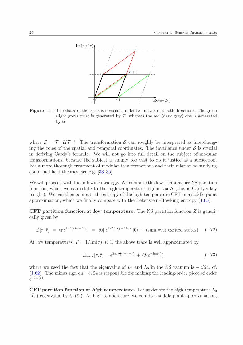
Figure 1.1: The shape of the torus is invariant under Dehn twists in both directions. The green(light grey) twist is generated by T , whereas the red (dark grey) one is generatedby U .

where S = T −1UT −1. The transformation S can roughly be interpreted as interchang-ing the roles of the spatial and temporal coordinates. The invariance under S is crucialin deriving Cardy’s formula. We will not go into full detail on the subject of modulartransformations, because the subject is simply too vast to do it justice as a subsection.For a more thorough treatment of modular transformations and their relation to studyingconformal field theories, see e.g. [33–35].

We will proceed with the following strategy. We compute the low-temperature NS partitionfunction, which we can relate to the high-temperature regime via S (this is Cardy’s keyinsight). We can then compute the entropy of the high-temperature CFT in a saddle-pointapproximation, which we finally compare with the Bekenstein–Hawking entropy (1.65).

CFT partition function at low temperature. The NS partition function Z is generi-cally given by

Z[τ, τ ] = tr e2πi (τL0−τ L0) = 〈0| e2πi (τL0−τ L0) |0〉 + (sum over excited states) (1.72)

At low temperatures, T = 1/Im(τ) ≪ 1, the above trace is well approximated by

Zlow-T [τ, τ ] = e2πic24

(−τ+τ) + O(e−Im(τ)) (1.73)

where we used the fact that the eigenvalue of L0 and L0 in the NS vacuum is −c/24, cf.(1.62). The minus sign on −c/24 is responsible for making the leading-order piece of ordere+Im(τ).

CFT partition function at high temperature. Let us denote the high-temperature L0

(L0) eigenvalue by ℓ0 (ℓ0). At high temperature, we can do a saddle-point approximation,

§1.4. Strominger’s Application of Cardy’s Formula 27

such that the leading-order behavior is given byiv

logZhigh-T [τ, τ ] ≃ S(ℓ0, ℓ0) + 2πi(

τℓ0 − τ ℓ0)

(1.74)

where ℓ0 and ℓ0 are functions of τ and τ , respectively, that extremize the right-hand side.This is an example of a Legendre transformation, which in this case replaces dependenceon ℓ0 (ℓ0) by dependence on τ (τ ).

Entropy. In order to get an expression for the entropy, one can do the inverse Legendretransformation

S(ℓ0, ℓ0) ≃ logZhigh-T [τ, τ ] − 2πi(

τℓ0 − τ ℓ0)

(1.75)

In this case, τ and τ are functions of ℓ0 and ℓ0 that extremize the right-hand side.

Like we mentioned above, the derivation of Cardy’s formula hinges on the fact that wehave modular invariance. This means explicitly that we can relate the above generalexpression for the high-T partition function to the one that is obtained from the modularlytransformed low-T partition function (1.73).

logZhigh-T [τ, τ ] ≃ logZlow-T [− 1τ,− 1

τ] = 2πi

c

24

(

1

τ− 1

τ

)

(1.76)

When we plug this into (1.75) we get

S(ℓ0, ℓ0) ≃ 2πic

24

(

1

τ− 1

τ

)

− 2πi(

τℓ0 − τ ℓ0)

(1.77)

Cardy’s formula. The last step in deriving Cardy’s formula is to extremize (1.77) withrespect to τ and τ and then to plug the result back into (1.77). We find the extremalvalues for τ and τ .

τ(ℓ0) = i

√

c

24ℓ0τ (ℓ0) = −i

√

c

24ℓ0(1.78)

We have chosen the signs for the roots such that the temperature 1/Im(τ) is positive.When we plug these back into (1.77) we finally arrive at Cardy’s formula.

S ≃ 2π

√

c

6ℓ0 + 2π

√

c

6ℓ0 (1.79)

ivTo see how the entropy S enters the story, it is nice to think of this trace in the following classicalsetting. When one diagonalizes the Hamiltonian H , the trace is just a sum over energy-eigenvalues ε. Thephase-space degeneracy is accounted for by the density of states ρ(ε) = eS(ε), i.e. ρ(ε) counts the numberof states with energy ε, which is exactly the logarithm of the entropy S(ε). Thus, the entropy enters theexponent through tr e−βH =

∫

dε eS−βε.


This formula, which was first found by Cardy [25], gives the entropy of a CFT in thehigh-temperature regime. The key in obtaining the Cardy formula is the fact that we havemodular invariance, which tells us in particular that we can relate a torus with modularparameter τ to one that has a modular parameter −1/τ , thus relating a theory at lowtemperature Im(τ) ∼ ∞ to one at high temperature Im(τ) ∼ 0.

Strominger’s application of Cardy’s formula. In Section 1.1 we saw that thermalAdS3 and the BTZ black hole can be derived from the same Killing–Cartan metric on thecoset SL2(C)/SU(2), cf. (1.12). Moreover, we saw in (1.28) that the modular parametersof their (conformal) boundaries are related by S : τ 7→ −1/τ , which is precisely the samerelation that we used in the above derivation of Cardy’s formula! All we need to donow is simply plug in the Brown–Henneaux central charge c = 3G/2ℓ and the L0 and L0

eigenvalues of BTZ from (1.66), ℓ0 = ℓM + J and ℓ0 = ℓM −J . The entropy from Cardy’sformula (1.79) is

S = 2π

√

ℓ

8G(ℓM + J) + 2π

√

ℓ

8G(ℓM − J) (1.80)

which is exactly the same as the Bekenstein–Hawking entropy from (1.65).

In conclusion, we find precise agreement between the entropy calculated from the conformalfield theory side and from the gravity side.

SCardy = SBekenstein–Hawking (1.81)

This result is striking mainly because of the vastly different way the separate sides areobtained. It hints at a full duality between quantum gravity in asymptotically AdS3

spaces and (super)conformal field theories defined on its conformal boundary, althoughsuch a complete duality at the level of partition functions is not (yet) proved, see e.g. [36].

Chapter 2

Holographic Renormalization inHamilton–Jacobi Formalism

Holographic renormalization. In this chapter we will review various aspects of holo-graphic renormalization. As the title of the chapter suggests, we will work in the Hamilton–Jacobi canonical formalism. As we discussed in the Introduction on page 7, the idea ofholographic renormalization is basically to compute correlators in the strongly-coupled fieldtheory on the boundary and remove its UV divergences by removing the corresponding IR(large-r) divergences on the gravity side of the correspondence.

One can move away from the conformally-invariant fixed point by turning on finite (relevantor marginal) perturbations on the boundary. According to the holographic dictionary,such perturbations are sourced by normalizable modes of the classical fields in the bulk.In practice, one adds matter fields like scalars, vectors etc. (depending on the desiredperturbation) to the gravitational action. The boundary is then put at a finite radiusr = r0, so that the divergences are exposed in terms of the regulator r0. The divergencesare subtracted by appropriate counterterms, so that finally the limit r0 → ∞ can be taken.

Structure of this chapter. We start off with a brief review of the application of theHamilton–Jacobi formalism to GR in Section 2.1. This includes a nice side track thatclosely resonates with the definition of the ADM mass at the end of Appendix D, which isbased on a seminal paper by Brown & York [32].

In Section 2.2, we review De Boer, Verlinde, and Verlinde’s Hamilton–Jacobi formulationof holographic renormalization [15], which includes a method for expanding the Hamiltonconstraint. As a nice warp-up example for the real stuff in Section 3.2, we calculate Brown& Henneaux’s AdS3 central charge c = 3G/2ℓ with the freshly acquired techniques.

There is a close connection between the radial coordinate r and the energy scale µ in the

30 Chapter 2. Holographic Renormalization in Hamilton–Jacobi Formalism

field theory on the (cut-off) boundary. In this sense, we expect that the radial flow in thebulk translates to an RG flow in the space of couplings on the boundary. This will be thetopic of Section 2.3.

§2.1. Hamilton–Jacobi Formulation of Gravity 31

2.1 Hamilton–Jacobi Formulation of Gravity

We will now introduce the Hamilton–Jacobi canonical formalism applied to gravity. Wehave included the Hamilton–Jacobi (HJ) formalism for a point-particle in Appendix B torefresh (or introduce) the reader’s knowlegde on the subject.

Φ(0)

Φ(r)

Φ(r) + δΦ(r)

r

r + δr

Figure 2.1: In this figure, Φ denotes the collection of fields like the metric tensor, form fieldsetc. The (active) variations of the fields Φ(r) → Φ(r) + δΦ(r) are induced by a(passive) variation of the foliation parameter r → r + δr.

Hamilton–Jacobi equation for gravity (temporal foliation). The HJ formalismappears to be tailor-made for describing bulk dynamics in terms of data on the boundary(and vice versa). A schematic view of the setup is shown in Figure 2.1. The Hamilton–Jacobi equations of motion for a classical point-particle are

H = −δScl

δt(2.1a)

pa =δScl

δqa(2.1b)

All the above quantities are evaluated at the varying endpoint t, cf. Appendix B. In generalrelativity, the above HJ equations (2.1) are generalized to

H = 0 (2.2a)

pab =1√q

δScl

δqab(2.2b)

which is depicted in Figure 2.2. The generalization of the second HJ equation (2.2b) israther obvious and taken from Brown & York’s paper [32]. In generalizing the first HJ


equation, one might have expected something like H = −δScl/δt. The foliation parametert, however, does not have an absolute meaning because of general covariance (as opposedto the classical case). This means that δScl/δt must vanish for generally covariant theoriesand we are left with the constraint H = 0.

pab

HΣf

Figure 2.2: A pictorial motivation of the generalized HJ equations; f = t for a temporal foli-ation and f = r for a radial one (cf. Appendix D). The momentum pab generatestransformations tangent to Σf , while H generates (in principle) a flow along theflow vector fµ. This is matches the nature of the point-particle’s HJ formalism, cf.Appendix B.

A radial foliation. We now turn to De Boer, Verlinde, and Verlinde’s (dBVV) radialfoliation [15], cf. Appendix D. In dBVV’s Hamilton–Jacobi method of holographic renor-malization, the radial coordinate gets the special role that is usually laid out for the timecoordinate. So, instead of studying the dynamics of time-like hypersurfaces like ADM did,dBVV studied radial evolution of equal-r slices. Note that by an ‘equal-r slice’, we mean ahypersurface whose embedding constraint, φ = constant, is given by φ(xµ) = r.i A genericmetric is then written as

ds2 = N2dr2 + qab(dya +Nadr)(dyb +N bdr) (2.3)

where qab is the induced metric along the equal-r hypersurface Σr, which generally dependson both the foliation parameter r and the intrinsic coordinates ya. We may always fix thegauge by setting the lapse and shift to some specified values, the most common one beingN = 1 and Na = 0. The radial dBVV Hamiltonian will then correspond to a radialflow rµ = N nµ +Na eµa instead of the standard ADM Hamiltonian’s time-like flow tµ. Inmost cases, the radial coordinate (foliation parameter) r is chosen to be the logarithm of a

iSee Appendix D if this does not sound familiar.

§2.1. Hamilton–Jacobi Formulation of Gravity 33

‘proper’ radial coordinate, such that the AdS metric is given in terms of Gaussian normalcoordinates. At large r, the metric tends to

ds2 = dr2 + e2r/ℓ ηab dyadyb (2.4)

which means that shifting r 7→ r + a acts as a rigid scaling on the hypersurface and thedBVV Hamiltonian can be seen as the generator of such shifts.

The Hamilton–Jacobi equations. Let us formally denote the collection of fields by Φ.The way the HJ equations are usually written down is obtained by plugging the second HJequation into the first, i.e.

H(Φ, δScl

δΦ, r) = 0 with H =

∫

Σt

ddy√q(

N H +Na Ha

)

(2.5)

Solving the HJ equation comes down to solving the radial Hamilton and momentum con-straints, H = 0 and Ha = 0, cf. Appendix D. The momentum constraint is exactly therequirement that the boundary (Brown–York) stress tensor (1.51) is conserved on shell,ii

0 = Ha = 2∇b pab = ∇b τab (2.6)

In other words, the momentum constraint requires that the on-shell action is invariantunder local diffeomorphisms on the hypersurface Σr, which can be automatically satisfiedby choosing a suitable Ansatz. The name of the game is to solve the Hamilton constraint,

H(Φ, δScl

δΦ, r) = 0 (2.7)

In principle, there are still surface terms that need to be taken into account. However, weassume the hypersurface Σr to be compact (∂Σr = ∅) throughout this chapter, so that weneed not worry about surface terms.iii

iiThe momentum contraint contains more terms in the presence of matter fields, see e.g. (D.26) and(D.33).

iiiFor example, we could assume that the induced metric qab has Euclidean signature. The topology ofthe d-dimensional hypersurface Σr (r ∼ ∞) at finite temperature is S1 × Sd−1. In Lorentzian signature,we would get a surface term proportional to the trace of the extrinsic curvature on ∂Σr at t = ±∞, whichis closely related the ADM mass term in (D.16). There is, of course, a whole array of additional issueswhen one works in Lorentzian signature, cf. [37].


2.2 Expanding The Hamilton Constraint

We will now discuss De Boer, Verlinde, and Verlinde’s (dBVV) approach to holographicrenormalization [8, 15], which was refined and extended in e.g. [38–40].

Splitting up the on-shell action. We will now proceed with dBVV’s analysis of solvingthe Hamilton–Jacobi equation (2.5) in the holographic context. An important assumptionthat we will make is one may split up the on-shell action as Scl = Sloc + Γ, where Sloc con-tains only local power-law divergent terms and Γ contains the remainder. This non-localremainder will turn out to comprise the effective action of the theory on the cut-off bound-ary. Γ has no power-law divergences (by definition), but it may still be logarithmicallydivergent. The regularization of Γ is fairly straightforward and, in fact, it turns out to beinessential for determining the conformal anomaly.

Premises for a derivative expansion. It is very useful to do a derivative expansionin order for the calculation to be manageable. We expand the local piece in the on-shellaction, such thati

Scl = S(0)loc + S

(2)loc + · · ·+ S

(d)loc + Γ (2.8)

where d+ 1 is the number of spacetime dimensions. The term S(d)loc is only there when d is

even.ii We shall use the following premises for expanding the Hamilton constraint.

1. S(n)loc contains all terms that involve n derivatives ∂a.

iii

2. Sloc consists of only local covariant (and gauge-invariant) expressions in terms of thefields and their derivatives at the cut-off boundary.

3. Sloc contains all power-law divergences Scl.

4. Sloc is universal, i.e. it has the same form for any solution with the same asymptotics.

These are basically Martelli & Muck’s expansion premises [39], except for the first one.

Their first premise reads “S(n)loc has exactly n/2 inverse (induced) metrics”. The reason for

iThere is a subtle difference between our convention for what Γ is, which comes from [39], and the

convention from dBVV’s original paper [15]. The two are related through ΓdBVV = Γ+ S(d)loc .

iiThe reason why the expansion of Sloc is only done up to level d has to with the fact that we implicitlyassume that our space tends to AdS at r ∼ ∞. Namely, the volume form (read:

√q) asymptotically goes

as ed r/ℓ for AdSd+1. For odd d, Sd−1loc is the last term.

iiiThis premise may seem too restrictive for us to also apply to anisotropically-scaling spacetimes. How-ever, in the next section we will explicitly show that there is no real obstruction when the space asymptotesto Lifshitz spacetime.

§2.2. Expanding The Hamilton Constraint 35

not picking this method of expanding is simply that it does not reproduce the requiredresult when we consider asymptotically Lifshitz spacetimes in Section 3.2.

The (cut-off) boundary momenta Π(x), conjugate to the fields Φ(x) at the boundary, aregiven in terms a derivative of the on-shell action with respect to the fields themselves (notΦ).

Π∣

∣

Σr=

1√q

δSloc

δΦ

∣

∣

∣

∣

Σr

(2.9)

which is similar to (B.5). The above expansion naturally induces an expansion for Π,

Π = Π(0) +Π(2) + · · ·+Π(d) +Π(Γ) (2.10)

To be more specific, the fields that one typically encounters (apart from fermions) are theinduced metric qab, a scalar φ, and a one-form Aa. Their respective canonical momentaare

pab =1√q

δScl

δqabπ =

1√q

δScl

δφEa =

1√q

δScl

δAa(2.11)

The full Hamilton constraint is given in (D.34), which can also be expanded with the abovepremises,

H = H(0) +H(2) + · · ·+H(d) +H(Γ) (2.12)

The contribution at level n = 2k is given by

H(n) =∑

i+j=n

{

−2κ(

qacqbd − 1d−1

qabqcd)

p(i)ab p

(j)cd − 1

2π(i)π(j) − 1

2E(i)aE(j)

a

}

− L(n)

(2.13)

where L(n) is the nth-level term in the expansion for the Lagrangian restricted to the bound-ary. This boundary Lagrangian plays the role of the potential in the (radial) Hamiltonian;it is defined to contain all of the non-‘kinetic’ terms (no radial derivatives or their associatedmomenta).

L =1

2κ

(

R− 2Λ)

+ Lmatter (2.14)

Check out (D.34) to see what Lmatter is for a self-interacting scalar and a massive vector.Keep in mind that, unlike in the original ADM picture, the ‘dynamics’ is actually in termsof radial (not temporal) evolution. One should beware of the fact that the crossterms in(2.13), i.e. terms with i 6= j, appear twice.


The last thing that we need is an expression for H(Γ) from (2.12). We use the fact that

Γ has the same power-law behavior as S(d)loc by construction (even though it may also be

logarithmically divergent). We thus get H(Γ) by combining Γ and S(0)loc in (2.13), i.e.

H(Γ) = −4κ(

qacqbd − 1

d− 1qabqcd

)

p(0)ab p

(Γ)cd − π(0)π(Γ) − E(0) aE(Γ)

a (2.15)

It should be clear that there is no such thing as L(Γ).

Warm-up example: pure gravity in 3 spacetime dimensions. Let us work out asimple example to see how the formalism that we have just laid out works in practice. TheAnsatz for Sloc for pure gravity in d + 1 = 3 spacetime dimension that is compatible withthe above premises is (in the pure-radial gauge N = 1, Na = 0)

Sloc =1

2κ

∫

Σr′

d2y√q {c1 + c2R + . . .} (2.16)

where ci ∈ R. The boundary Lagrangian is simply L = (R − 2Λ)/2κ. The expansion forSloc and L is

S(0)loc =

1

2κ

∫

d2y√q c1 L(0) = −Λ

κ(2.17a)

S(2)loc =

1

2κ

∫

d2y√q c2R L(2) =

R

2κ(2.17b)

The only canonical momentum that we need to compute is pab, whose expansion followsfrom plugging the expanded Scl into (2.11).

p(0)ab = − c1

4κqab p

(2)ab =

c22κ

(

Rab −1

2qabR

)

(2.18)

When we plug these into the expanded Hamilton constraint (2.13), we get

H(0) =1

2κ

(

c212+ 2Λ

)

H(2) = − 1

2κR (2.19)

The Hamilton constraint H = 0 is satisfied at level zero if we let c1 = −2√−Λ = −2/ℓ,

where ℓ is the AdS curvature radius like we had before.iv At second level, though, weimmediately see a problem arising. Namely, there is no dependence on c1 or c2 in H(2),which means that we cannot put it to zero in the same way. This is where the effectiveboundary action Γ comes into play. Notice that the full expansion in 3 dimensions is

H = H(0) +H(2) +H(Γ) (2.20)

ivWe chose the negative root so that Scl has a negative cosmological constant.

§2.2. Expanding The Hamilton Constraint 37

so we note that Γ should be such that H(Γ) = −H(2), which implies thatv

qab2√q

δΓ

δqab= − ℓ

16πGR (2.21)

We recognize the trace of our (unregulated) boundary stress tensor on the left-hand side,so we see that this is the familiar expression of the Weyl anomaly in a two-dimensionalCFT. We get the central charge c by relating this to the standard form T a

a = −(c/24π)R,so that we find

c =3ℓ

2G(2.22)

which is the exact same central charge that we got from the Brown–Henneaux procedurein the previous chapter, which is a nice consistency check.

Logarithmic divergence. We were a little hasty in calling Γ the effective boundaryaction. We should have made sure that it has no logarithmic divergence first.vi To revealany logarithmic dependence in Γ, one can do an infinitesimal rescaling r → r + ε, see e.g.[39]. The difference is

Γ(r + ε)− Γ(r) = ε

∫

d2y (∂rqab)δΓ

δqab+O(ε2)

=ε

ℓ

∫

d2y 2qabδΓ

δqab+O(ε2)

= −ε

∫

d2y√qH(Γ) +O(ε2) ⇒ ∂rΓ ≃ −

∫

d2y√qH(Γ)

(2.23)

We used that the induced metric asymptotes to AdS at r ∼ ∞, from which it follows that∂rq

ab ≃ (2/ℓ) qab. The anomalous piece of the Hamilton constraint H(Γ) is proportional tothe Ricci scalar and it is well known that the combination

√qR is Weyl invariant in two

dimensions, thus also independent of r (to leading order).vii The above expression can thenbe integrated to get

Γ = −r

∫

d2y√qH(Γ) + (finite piece) (2.24)

The renormalized effective boundary action is obtained by

Γren = limr→∞

{

Γ + r

∫

d2y√qH(Γ)

}

(2.25)

vWe use the notation κ ≡ 8πG, cf. Appendix C.viBy ‘logarithmic’, we mean logarithmic in er/ℓ, which is the same as power-law in r. The transformation

r → r + λ looks like a translation in terms of r, but it is of course a dilatation when exponentiated.viiThe anomalous Hamilton constraint has a different form in a higher number of dimensions, but the

fact that√qH(Γ) is Weyl invariant remains true.


The metric and the anomalous Hamilton constraint can be renormalized by rescaling it as

qab → qren

ab = limr→∞

e−2r/ℓ qab and H(Γ) → H(Γ)ren

= limr→∞

e2r/ℓ H(Γ)(2.26)

The proper Weyl anomaly is then given by

qabren

2√qren

δΓren

δqabren

= − ℓ

16πGR[qren] (2.27)

which gives the same central charge as before. The reason for the coincidental answers ofthe renormalized and unrenormalized anomalies can be seen related to the fact that bothsides of the unrenormalized anomaly are precisely equally divergent, a fact that may notbe generically true.

§2.3. From Radial to RG Flow 39

2.3 From Radial to RG Flow

The study of holographic RG flows relies on the identification of two seemingly distinctnotions of flow: the radial flow in the bulk gravity theory and the RG flow in the effective(cut-off) boundary theory. This identification follows from the standard AdS/CFT dictio-nary, which in particular states that the IR of the bulk theory corresponds to the UV onthe boundary (and vice versa) [7]. In other words, the RG scale of the effective theory thatlives on Σr goes as µ ∼ er/ℓ at r ∼ ∞. In this section we will make a precise connectionbetween the radial flow in the bulk and RG flow on the boundary.

Domain-wall geometries. We will now study the radial evolution of so-called domainwall solutions. The metric is a generalization of the AdS metric (2.4) given in terms ofsome function f(r).

ds2 = dr2 + ef(r) ηab dyadyb (2.28)

AdS obviously corresponds to f(r) = 2r/ℓ. The above metric is a solution to the fieldequations that come from varying the action

S = Sgrav + Sφ =

∫

M

dd+1x√g

{

1

2κ

(

R− 2Λ)

− 1

2∂µφ ∂µφ− V (φ)

}

+1

2κ

∮

∂M

ddy√q 2K

(2.29)

Given that the potential can be written in terms of some other function of the scalar U(φ)according to

V (φ) = (...)U ′(φ)2 − (...)U(φ)2 (2.30a)

the field equations are

φ = (...)U ′(φ) f = (...)U(φ) (2.30b)

The ellipses represent numerical factors and by the dot on e.g. φ we mean Lie differentiationalong the radial flow vector rµ∂µ, which is just (logarithmic) radial differentiation ∂r in thepure-radial gauge N = 1, Na = 0. We will now show these equations are easily obtainedwith the HJ method laid out in the previous two sections.

Solving the Hamilton constraint. We set out to solve the Hamilton constraint comingfrom the above action (2.29). The boundary Lagrangian is L = Lgrav +Lφ, which are givenin (D.34) by

Lgrav =1

2κ

∫

Σr

ddy√q{

R− 2Λ}

(2.31a)

Lφ = −∫

Σr

ddy√q

{

1

2∂aφ ∂aφ+ V (φ)

}

(2.31b)


The Ansatz for the local part of the on-shell action follows from the premises on page 34.

Sloc =

∫

Σr

ddy√q {U + ΦR +M ∂aφ ∂aφ+ . . .} (2.32)

where U(φ), Φ(φ), and M(φ) are ordinary functions of φ. We truncated the series in sucha way that we can read off the first two levels in the derivative-like expansion. This doesnot mean that we have all the information that we need in any number of dimensions d,but it will suffice for deriving (2.30). The expansion for the boundary Lagrangian (2.31)and the local on-shell action Sloc also follow from the premises.

S(0)loc =

∫

ddy√q U L(0) = −Λ

κ+ V (φ) (2.33a)

S(2)loc =

∫

ddy√q{

ΦR +M ∂aφ∂aφ}

L(2) =R

2κ− 1

2∂aφ ∂aφ (2.33b)

The canonical momenta at lowest (most divergent) level are

p(0)ab = −1

2qab U π(0) = U ′ (2.34)

and at second level, they are

p(2)ab = Φ

(

Rab − 12qab R

)

+(

M − Φ′′)∂aφ ∂bφ+(

− 12M + Φ′′)qab ∂cφ ∂cφ

+ Φ′(qab∇c∇c −∇(a∇b)

)

φ

π(2) = Φ′ R +M ′ ∂aφ ∂aφ+ 2M ∇a∇aφ

(2.35)

When we plug these into the expanded Hamilton constraint (2.13), up to level two, we get

H(0) = d2d−2

κU2 − 12(U ′)2 + V (φ) (2.36a)

H(2) =[

d−2d−1

κUΦ− U ′Φ′ − 12κ

]

R

+ [−2κUΦ′ − 2U ′M ] ∇a∇aφ

+[

d−2d−1

κUM − 2κUΦ′′ − U ′M ′ + 12

]

∂aφ ∂aφ

(2.36b)

We see that the level-zero Hamilton constraint H(0) = 0 yields the (fake) superpotentialrelation (2.30a). The field equations (2.30b) are directly obtained from the Hamiltonequation q = ∂H/∂p at the boundary, i.e. with the momenta given by (2.11).

φ = π ≈ U ′ qab = −4κ(

pab − 1d−1

qab p)

≈ −2κU qab (2.37)

The first field equation in (2.30b) is indeed already sitting there. The second one comesfrom noticing that the domain-wall metric (2.28) implies qab = f qab.

§2.3. From Radial to RG Flow 41

The Callan–Symanzik equation. In order to complete the connection between theradial flow and boundary RG flow we will now review a derivation of the Callan–Symanzikequation from purely holographic reasoning. Because it is not essential for the remainderof this text, our treatment will be rather shallow, see [8] for a more complete analysis.The derivation requires the ‘AdS/CFT master equation’ (see e.g. [2]), which relates theeffective action Γ to the generating functional of the boundary CFT. It formally looks like

Γ[Φ] =⟨

e∫ddy

√qΦ·O

⟩

bndy

(2.38)

This Γ is the same one as Γ = Scl −Sloc that we saw before. In [8], the notion of a physicalscale µ = exp f(r) is introduced, such that qab = µ δab. Via (2.37) we see that µ = −2κU µ.The beta function for φ is then defined as the usual logarithmic derivative

βφ ≡ µ∂

∂µφ =

1

2κ

U ′

U(2.39)

where we assumed that f(r) is invertible. We use (2.38) together with the commutationrelation [ΦI , δ/δΦJ] = −δIJ to arrive at the Callan–Symanzik equation

(

µ∂

∂µ+ βφ

∂

∂φ

)

〈O(y1) · · ·O(yn)〉+n

∑

i=1

γi 〈O(y1) · · ·O(yi) · · ·O(yn)〉 (2.40)

where γi is the anomalous dimension of the operator O(yi) which is sourced by φ(yi).Admittedly, we have been rather sloppy in this last paragraph. For instance, we havenot properly defined the partial derivatives. Again, we refer the reader to De Boer’slecture notes on HJ holography [8] for a more thorough treatment of this topic. In theselecture notes, an arbitrary number of scalars is taken, which is closer to the nature of therenormalization group, since one typically has a space of couplings that has more thanone dimension. The result is very nice nonetheless; we explicitly see a strong result fromordinary RG arise by just plugging in the level-zero Hamilton constraint. Of course, the‘AdS/CFT master equation’ appeared somewhat mysteriously and has not been justified.However, a satisfactory justification of it is beyond the scope of this thesis.

Chapter 3

Lifshitz/Schrodinger Asymptotics

Schrodinger spacetime. Over the past two years or so, there has been a lot of interestin extending the well-known AdS/CFT correspondence [1–3] to condensed matter appli-cations, see e.g. [41–43] for an overview. A subclass of these so-called AdS/CMT set-upsconsists of using holographic duals to study theories at a Schrodinger-invariant UV fixedpoint.i By Schrodinger-invariant we mean invariant under the group of symmetries of thefree Schrodinger equation i∂t = −∇2/2m. This so-called Schrodinger group is introduced inSection 3.1. Son [10] and (Koushik) Balasubramanian & McGreevy [11] published their pa-pers on so-called Schrodinger spacetime around the same time. The metric on Schrodingerspacetime typically looks like

ds2 = −r4 dt2 +dr2

r2+ r2

(

2dξ dt+ d~x2)

(3.1)

which can be obtained by some discrete light-cone quantization (DLCQ) procedure [44].The isometry group of (3.1) is the Schrodinger group. In fact, the metric (3.1) was derivedfrom the observation that the Schrodinger group is the DLCQ of the Poincare group [10].One of the standard properties of holographic dualities is that they relate theories of co-dimension one. Because of this DLCQ procedure, the duality is between two theoriesof co-dimension two (the ξ coordinate gets interpreted as the particle number densityoperator M). This is reminiscent of the study of null hypersurfaces in standard GR. Insome cases such as [11], a generic value for the so-called dynamical critical exponent z isallowed. The critical dynamical exponent gives us a measure for anisotropy in the scalingbehavior. In other words, a system that scales anisotropically with z 6= 1 is invariant undersimultaneously rescaling xi 7→ λxi and t 7→ λzt. The critical dynamical exponent roughlyenters the dispersion relation as H ∼ P z; we will focus on the case where z = 2. The storyof Schrodinger spacetimes was further developed in e.g. [12, 45, 46].

iKeep in mind that holographic dualities typically relate the UV of the boundary theory to the IR ofthe bulk theory.

44 Chapter 3. Lifshitz/Schrodinger Asymptotics

This chapter is a first step towards a new way of looking at Schrodinger holography. Themain idea is the following.ii In a conformal field theory, the conformal algebra picks up afinite central charge upon quantization. This central charge for AdS3 was obtained in theprevious two chapters using two distinct methods, which both led to c = 3ℓ/2G. Similarly,in a theory with Schrodinger symmetry, the Schrodinger algebra also has a central charge.This time, the central charge is the mass density operator, which for example can bethe mass m that appears in the Schrodinger equation i∂t = −∇2/2m. An importantimplication of viewing the mass density operator as a central charge is that it removes theneed for having the extra ξ dimension.

The first attempt towards finding a finite central charge M is by use of the Brown–Henneaux procedure from Chapter 1, which is pursued in Section 3.1. The second attempt,in Section 3.2, is made by using holographic renormalization techniques from Chapter 2.In both cases, we will not work with Schrodinger spacetime, but with so-called Lifshitzspacetime [9], given by

ds2 = −r4 dt2 +dr2

r2+ r2 d~x2 (3.2)

i.e. discarding the ξ direction and thus turning the holographic duality back into a codimension-one duality. In contrast to Schrodinger spacetime (3.1), the Lifshitz geometry does not haveGalilean boosts K : x 7→ x+ vt as an isometry.

Why Lifshitz spacetime? The reason for using Lifshitz instead of Schrodinger has todo with the fact that we do not need (or want) the Galilean boosts to be exact symmetriesof our background. Namely, as we will discuss in Section 3.1, one can only obtain a centralcharge c from [A,B] = c if both A and B are not exact isometries. The central chargethat we will be looking for comes from the commutator of a Galilean boost K and aspatial translation P , i.e. [K,P ] = M . This means that both K and P cannot be exactKilling symmetries of (3.2). Hence, losing Galilean boosts when choosing Lifshitz in favorof Schrodinger is not a bad thing; it is required. We must, of course, also break spatial-translation invariance. Moreover, it must also be shown that K and P are still approximate(asymptotic) symmetries. We will discuss these issues in Section 3.1.

A disclaimer. The topics in this chapter are work in progress. The notes in red are thepoints that I’m still working on. Even though I have not finished the analysis, I would stilllike to share some of my thoughts on these subjects.

iiThis is Prof. Maloney’s idea.

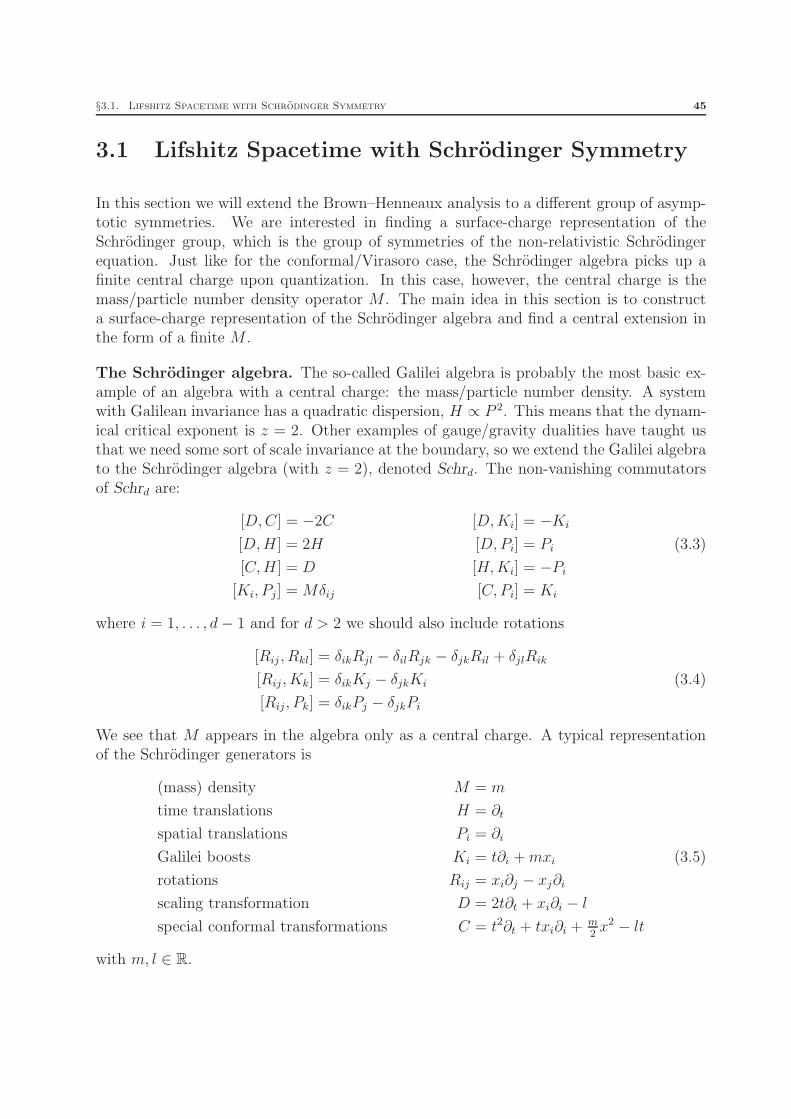
§3.1. Lifshitz Spacetime with Schrodinger Symmetry 45

3.1 Lifshitz Spacetime with Schrodinger Symmetry

In this section we will extend the Brown–Henneaux analysis to a different group of asymp-totic symmetries. We are interested in finding a surface-charge representation of theSchrodinger group, which is the group of symmetries of the non-relativistic Schrodingerequation. Just like for the conformal/Virasoro case, the Schrodinger algebra picks up afinite central charge upon quantization. In this case, however, the central charge is themass/particle number density operator M . The main idea in this section is to constructa surface-charge representation of the Schrodinger algebra and find a central extension inthe form of a finite M .

The Schrodinger algebra. The so-called Galilei algebra is probably the most basic ex-ample of an algebra with a central charge: the mass/particle number density. A systemwith Galilean invariance has a quadratic dispersion, H ∝ P 2. This means that the dynam-ical critical exponent is z = 2. Other examples of gauge/gravity dualities have taught usthat we need some sort of scale invariance at the boundary, so we extend the Galilei algebrato the Schrodinger algebra (with z = 2), denoted Schrd. The non-vanishing commutatorsof Schrd are:

[D,C] = −2C [D,Ki] = −Ki

[D,H ] = 2H [D,Pi] = Pi (3.3)

[C,H ] = D [H,Ki] = −Pi

[Ki, Pj] = Mδij [C, Pi] = Ki

where i = 1, . . . , d− 1 and for d > 2 we should also include rotations

[Rij , Rkl] = δikRjl − δilRjk − δjkRil + δjlRik

[Rij , Kk] = δikKj − δjkKi (3.4)

[Rij, Pk] = δikPj − δjkPi

We see that M appears in the algebra only as a central charge. A typical representationof the Schrodinger generators is

(mass) density M = m

time translations H = ∂t

spatial translations Pi = ∂i

Galilei boosts Ki = t∂i +mxi (3.5)

rotations Rij = xi∂j − xj∂i

scaling transformation D = 2t∂t + xi∂i − l

special conformal transformations C = t2∂t + txi∂i +m2x2 − lt

with m, l ∈ R.


Asymptotically Lifshitz spacetimes. We are looking for a spacetime that, first ofall, is physical. In other words, it should consistently solve the field equations of sometheory. On top of that, the asymptotic symmetry algebra of the metric should contain theSchrodinger algebra. Like we mentioned before, we are looking to find the (mass) densityoperator from the Poisson (Dirac) bracket {QKi

, QPj} = Mδij . As was noted in [16], there

is an important restriction to the metrics that we are allowed to choose. If the asymptoticsymmetries are exact isometries of the background space M, all central charges vanishexactly. In other words, if either ζ or η sits in iso(M), all Cζη vanish. To see this, we notethat the central charge from (1.42),

Cζη = Qζ [Lηg] = −Qη[Lζ g]

vanishes because the Lie derivative of the metric with respect to an isometry vanishesidentically (by definition).

We will thus look for a background geometry M such that the algebra of its isomorphisms isa proper subalgebra of the asymptotic symmetry algebra, i.e. iso(M) ⊂ asg(M). Anotherthing we are looking for is the property that the asymptotic symmetry algebra covers theSchrodinger algebra, i.e. Schrd ⊆ asg(M). In summary, we would like to have the followinghierarchy of algebras.

iso(M) ⊂ Schrd ⊆ asg(M) (3.6)

and the generators whose brackets ought to give the central charge must sit in the coset

Schrd/iso(M) (3.7)

The Lifshitz background Ansatz. Motivated by the above criteria, we choose a slightlyadjusted version of Kachru, Liu, and Mulligan’s [9] Lifshitz spacetime solution for ourbackground.

gµν dxµdxν = −

(

r4 +r2

x2 + y2

)

dt2 +dr2

r2+ r2

(

dx2 + dy2)

(3.8)

We adjustment is the second term in gtt, which was put there in order to break the sym-metry under spatial translations generated by P . The isometries of (3.8) are {H,D,C},which span a subgroup of the Schrodinger group. Interestingly, this subgroup is isomorphicto the Mobius group SL2(R). The metric (3.8) should be a solution to the Einstein–Procaaction

∫

dr (Lgrav + LA) (cf. (D.16) and (D.30)), together the corresponding Proca field

Aµ dxµ = r2 dt (3.9)

These don’t solve the field equations! Maybe drop the r4 term in gtt? (this would mostlikely change the ASG too)

§3.1. Lifshitz Spacetime with Schrodinger Symmetry 47

Killing’s equation is solved in the asymptotic region r ∼ ∞ by any ξ that is of the form

ξ = f i,i ∂t + f i

,t ∂i −1

2f i

,it r∂r (3.10)

where f is an arbitrary function of xi = (x, y) and t only. In order to see that the asymptoticsymmetry group contains the Schrodinger algebra, we write f(x, t) as a power series in x

f i(x, t) = f i(0, t) + f i,j(0, t) x

j +1

2!f i

,jk(0, t) xjxk + . . . (3.11)

In the temporal foliation that will follow, we can choose to put our hypersurface Σt at anyvalue of t. We expand the function f(x, t) around t = 0 up to second order. We see thatthe piece linear in xi already contains all Schrodinger generators. We use the coefficientssuch that the connection with the corresponding Schrodinger generators (3.5) is clear. Forexample, the coefficient H ∈ R corresponds to the generator H = ∂t.

i

f i(x, t) = const. + P i t+Ki t2 +[

H + (D δij +R ǫij)t+ (C δij + .. ǫij)t2]

xj + . . . (3.12)

The main thing that should be taken from this expression is that the asymptotic symmetrygroup contains the Schrodinger group.ii We see in particular that the Galilean boosts andspatial translations emerge as symmetries at the asymptotic level, even though they arenot isometries. This means that the criteria (3.6) are indeed satisfied.

Asymptotically Lifshitz boundary conditions. Let us define (locally) asymptoticallyLifshitz spacetime to be a spacetime whose metric gµν = gµν + hµν respect the asymptoticboundary conditions,

(hµν) =

htt htr htx hty

hrr hrx hry

hxx hxy

hyy

=

O(r2) O(r−1) O(r2) O(r2)O(r−2) O(r−1) O(r−1)

O(r2) O(r2)O(r2)

(3.13)

Comparing these to the background metric itself at r ∼ ∞,

(gµν) ≈

−r4 0 0 0r−2 0 0

r2 0r2

(3.14)

we see that the deviations are not necessarily subleading. This is no real obstruction, forexample, this is also the case in Strominger et al.’s Kerr/CFT paper [47]. These boundary

iTo be more precise, ξ ∝ ∂t is obtained by setting all coefficients but H ∈ R to zero.iiFor those who are interested, we see in (3.10) that ξi = f i(0, t)+ f(0, t)i,jx

j + .. . The matrix f(0, t)i,j

is then decomposed into its trace ∼ δij , anti-symmetric ∼ ǫij , and traceless-symmetric ∼ σij pieces. Thelatter of which does not contribute, because it only appears contracted with the vector xi. (By the way, Idon’t know what the .. ǫij in the last term corresponds to (its corresponding generator is txi∂j − txj∂i).)


conditions are chosen such that any ξ of the form (3.10) is an asymptotic symmetry (att ∼ 0), which obviously includes the Schrodinger transformations (3.12). The boundaryconditions are obtained by relating hµν ∼ Lξgµν . This however, does not yield a boundarycondition for hrr, because Lξgrr vanishes identically for all ξ. Using the fact that theasymptotic symmetries should map the deviations onto themselves, hµν ∼ Lξhµν , willthen give the hrr boundary condition.

Since Lifshitz spacetime is not a solution to pure Einstein, but rather Einstein–Proca, weneed to do the same for the Proca field as well. The boundary conditions for the deviationsαµ = Aµ − Aµ read

(αµ) =(

αt αr αx αy

)

=(

O(r2) O(r3) O(r2) O(r2))

(3.15)

where, similar to the metric, the boundary condition for αt was obtained by requiringαµ ∼ Lξαµ.

Einstein–Proca surface charges on the Lifshitz background. We must add thecontribution from the Proca field Aµ to the surface charges Qζ(h). Using the Proca Hamil-tonian (D.33), our best guess at what the surface charge looks like is

Qζ(h) =

∮

∂Σt(∞)

dσa

{

1

2κGabcd

[

∇bhcd − hcd∇b

]

ζ + 2pab ζb + EaN ζ + EaAbζb

}

(3.16)

Before I start computing charges, I need to get the following issue out of the way. Namely,there is something terribly wrong with the above boundary conditions: they allow fordeviations htt from the background (3.8) at order r2, which means that the term that weneed in order to break the invariance under spatial translations can be ‘gauged away’. To bemore specific, the integration δQ → Q allows us to pick any background that is consistentwith the boundary conditions (3.13). Consequently, the (possible) central charge shouldnot depend on which one of these backgrounds we pick. In particular, we can pick KLM’sLifshitz spacetime (which is Pi-invariant), so the central charge M must be zero.

I have been playing around trying to fix this issue by making sure that P -invariance isbroken a leading order, but I have not yet found such a metric (+ Proca field) with thisproperty that solve the field equations (and still has an ASG that contains the Schrodingergroup). Though I feel like it’s not impossible...

§3.2. Holographic Renormalization of Lifshitz 49

3.2 Holographic Renormalization of Lifshitz

In view of the previous section, one would like to find a term in the on-shell action thatwould source the mass density operator proportional to [Ki, Pj]. However, for now we willbe satisfied with finding out the structure of the local counterterms sitting in Sloc for theEinstein–Proca action

∫

dr (Lgrav +LA). We will compare a simple result with that of Ross& Saremi [13] as a consistency check.

An additional effective dimension. The expansion truncates at marginal level S(d)loc

in the case of AdSd+1, (d even). This has to do with the fact that the volume form ofAdSd+1 scales as

√g ∼ ed r (the lapse scales as 1) in the asymptotic region. For KLM’s

d-dimensional Lifshitz spacetime [9] with z = 2, henceforth denoted Lifd,

ds2/ℓ2 = −r4 dt2 +dr2

r2+ r2 d~x2 with ~x ∈ R

d−2 (3.17)

or in Gaussian normal coordinates with ℓ = 1,

ds2 = dr2 − e4r dt2 + e2r d~x2 with ~x ∈ Rd−2 (3.18)

the volume form on Lifd scales as√g ∼ ed r, which is the same as AdSd+1. We will focus

on Lif4, which means that the expansion is truncated at S(4)loc , just like in AdS5. For this

reason, we could expect possible anomalous terms to appear, even though we are workingin an even number of spacetime dimensions.

Notice that the field content on this background inherits this additional effective dimension,so the analysis need not be altered in a very crude way. One may wonder, however, whetherfirst premise of the isotropic expansion on page 34 is justified. It turns out that it is, whichwe explain below.

Equivalence of isotropic and anisotropic expansion. The derivative expansion (page34) is inherently isotropic, i.e. it treats ∂t and ∂i on equal footing. Lifshitz spacetime, on theother hand, does not possess this isotropic property. We must thus show that expandingisotropically will yield the exact same equations as expanding anisotropically.

Let us temporarily alter the first expansion premise from page 34, such that it reflectsLifshitz’s anisotropy. The anisotropic premise would read

S(n) contains ns spatial and nt temporal derivatives in such a way that ns + 2nt = n.

Let us give a sketch of the reason why this anisotropic premise would still yield the sameequations in the expansion as the old isotropic one. This is most easily explained using theexample from Section 2.3. For conciseness, let us focus on the kinetic term of the scalar


field only.i

∂aφ ∂aφ = qtt (∂tφ)2 + qij ∂iφ ∂jφ (3.19)

These separate terms will respectively contribute at level 4 and 2 in the anisotropic ex-pansion. The Ansatz for the local piece of the on-shell action was given in (2.32). Let usinstead write down an Ansatz that is not necessarily isotropic,

Sloc = ... + M1(φ) ∂tφ ∂tφ + M2(φ) ∂iφ ∂iφ + ...

In turns out that the Hamilton constraint then contains two identical coefficients at differ-ent levels involving M1(φ) andM2(φ). The expanded Hamilton constraint that correspondsto the above Sloc looks like

ii

H(2) = ... +(

d−2d−1

κUM2 − 2κUΦ′′ − U ′M ′2 +

12

)

∂iφ ∂iφ + ...

H(4) = ... +(

d−2d−1

κUM1 − 2κUΦ′′ − U ′M ′1 +

12

)

∂tφ ∂tφ + ...

See (2.36b) for the same Hamilton constraint in the isotropic case. The main point isthis. We see that both M1 and M2 must solve the exact same constraint. Thus, restoringisotropy/Lorentz-invariance by setting M1 = M2 is obviously consistent and most likelyinevitable. So even if one were to choose an anisotropic Ansatz, Lorentz invariance isrestored by solving the Hamilton constraint.

There are two conclusions from this: the anisotropic expansion yields the same constraintsas the old isotropic one and Lorentz invariance pops up even if we allow for an anisotropicAnsatz. The fact that we have Lorentz invariance is not very surprising, because at finite rbulk covariance is still preserved. It is only in the limiting case r → ∞ that the (asymptotic)symmetry group changes. This is also related to Horava’s idea of a radially varying speedof light. For example, the metric on a radial hypersurface that is induced by pulling back(3.18) is invariant under Lorentz transformations where the speed of light is c = er, whichis finite at finite r.

Solving the Hamilton constraint for Lif 4. We will now move on to the main topicof this section. We would like to solve the Hamilton constraint coming from the Einstein–

iWe assume that we may consistently set the embedded shift to zero, N i = −qit/qtt = 0.iiIn order to arrive at this result, one needs to do an embedded temporal foliation, e.g. the Gauss–

Codazzi equations yield (d)R = (d−1)R− k2 + kijkij where kij ∼ ∂tγij is the embedded extrinsic curvature.


Proca action.iii

Sgrav + SA =

∫

M

dd+1x√g

{

R− 2Λ

2κ− 1

4FµνF

µν − m2

2AµA

µ

}

+1

2κ

∮

∂M

ddy√q 2K (3.20)

whose corresponding boundary Lagrangian is given by

Lgrav + LA =1

2κ

(

R− 2Λ)

− 1

4FabF

ab − m2

2AaA

a (3.21)

Let us introduce α ≡ −AaAa − 1, which is a deviation from the background of order

α ∼ O(e−2r), [13]. The deviation is defined such that α = 0 on the Lifshitz background.The most general Ansatz for the local-term action in terms of the canonical variables is

Sloc =

∫

Σr

ddy√q{

F (α) + (derivative terms)}

(3.22)

where we only wrote down the term that contributes to the Hamilton constraint level zero.iv

A consistency check. We will do a consistency check with a basic result from Ross &Saremi (RS) [13]; we check if their F (α) is compatible with ours. RS’s function F (α) (fromSection 2 of [13]) is given by

F (α) = −4− 2√−A2 = −4− 2

√α + 1 = −6− α+

1

4α2 + ... (3.23)

RS’s conventions are such that κ = 1/2, Λ = −5, and m = 2, which we will adopthenceforth.

At level zero (most divergent), we have

S(0)loc =

∫

ddy√q F (α) and L(0) = −Λ

κ+

m2

2(α + 1) (3.24)

The expanded momenta that follow from the above expansion are

p(0)ab = −1

2F (α) qab − AaAb F

′(α) and E(0)a = −2Aa F

′(α) (3.25)

iiiWe get rid of the N and ∇aEa terms in (D.34) by first integrating out N , which comes down to

substituting N = ∇aEa/m2. We choose our Ansatz for Sloc to be manifestly covariant, such that ∇bτab =

2∇bpab = 0. This is nice, because the momentum constraint yields

0 = Ha = −2∇bpab −Aa∇bEb = −Aa∇bE

b ⇒ ∇aEa = 0

I’m not very confident that this reasoning is valid.ivThe coefficients of the other terms are all functions of the Lorentz-scalar quantity α.


Instead of turning straight to the Hamilton constraint, we will start with the Hamiltonequation qab = δH/δpab at level zero,v

qLif

ab ≃ −2p(0)ab + p(0) qLif

ab (3.26)

where qLif

ab is the induced metric on the Lifshitz background, i.e. qLif

ab dyadyb = −e4t dt2 +

e2t d~x2. The tt-component and ij-components on the Lifshitz background (α = 0) respec-tively give

c0 + 2c1 + 8 = 0 and c0 − 2c1 + 4 = 0 (3.27)

which indeed return the expected values c0 = −6 and c1 = −1. The HJ method finallyproduces

F (α) = −6 − α + c2 α2 (3.28)

which agrees with (3.23). Remember that the deviations are of order α ∼ O(e−2r), whilethe volume form is of order

√q ∼ O(e4r). Thus, the term quadratic in α is marginal, which

means that fixing c0 and c1 suffices to remove the divergences. RS defined their F (α) forthis purpose only, so it would have sufficed to determine F (α) only up to linear order. Inother words, one can freely add to the action any term proportional to α2 = (AaA

a + 1)2.

How about the level-zero Hamilton constraint? We use the recipe outlined in Section 2.2to get

H(0) =3

8F 2 − 1

2(α+ 1)F ′F − 1

2(α2 − 2α− 3)(F ′)2 − 2α− 12 = 0 (3.29)

We assume that we may write the function as a power series,

F (α) = c0 + c1 α + c2 α2 + ... (3.30)

which we plug back into (3.29). At lowest level, we have

H(0) =3

8c20 −

1

2c0 c1 +

3

2c21 − 12 +

(

−(c0 − 6c1)c2 +1

4c0 c1 +

1

2c21 − 2

)

α + O(α2)

(3.31)

We now notice that when we plug in the values c0 = −6 and c1 = −1, the constant andlinear terms vanish identically.

H(0) = O(α2) (3.32)

vThe reason for doing this is that the Hamilton constraint turns out not to fix the value of c0. We willcheck the consistency of the level-zero Hamilton constraint shortly though.


So the Hamilton constraint is consistent with the answers that we got from the Hamiltonequation qab = δH/δpab. In principle, one can determine c2, c3, etc. from this, but likewe just mentioned this is not needed for removing divergences. Nevertheless, it would beinteresting to exactly obtain the square-root behavior from (3.23). However, one finds twopossible values c2 = −1

4and c2 =

512, which both do not fit RS’s c2 =

14.

Concluding remarks. We have managed thus far to construct a relatively systematicway to find the counterterms that cancel the UV divergences in a class of strongly coupledQFT’s at a fixed point that exhibit Lifshitz-like scaling. The analysis is of course farfrom complete and there is much to be done. For example, one should continue the aboveprogram at level two and four.

One could also try to see if one can get an actual RG flow by adding a scalar field to theProca–Einstein theory, which should give something analogous to (2.37) already at levelzero.

The initial objective to find an operator that corresponds to [K,P ] with a finite expectationvalue is also to be explored. It would be very interesting to find a Lifshitz analogue of AdS’sconformal anomaly.

Appendix

A Killing–Cartan Metrics

The metric on a compact simple Lie group manifold can be obtained from combininggroup elements into the product of two so-called bi-invariant Cartan one-forms. It shouldbe noted that this section is not intended as a thorough mathematical treatment of theabove statement. It mainly serves as a motivation for obtaining the generalized form ofthe (thermal) AdS3 and BTZ metrics discussed and their isometries in Section 1.1. Thedefinitions in this section are mostly taken from Chapter 18 and 21 of Frankel’s book [48].

Generalized action. There is a generalized notion of group-action on elements of the(co)tangent space about some point g on the group manifold. Such actions are sometimesreferred to as induced group-actions. Generalized left-action by some group element h ∈ Gdenoted as Lh. Note that the left-action is simply Lh(g) = hg when g ∈ G. However,instead of left-actions on the group itself, we can also consider the left-action on the tangentspace in g, so that Lh∗ : TgG → ThgG. This ∗ notation is used to keep in mind that it actsas a push-forward. Similarly, L∗

h : T ∗gG → T ∗

hgG acts on cotangent spaces as a pull-back.The right-action Rh is defined in an obviously similar fashion.

Maurer–Cartan forms. Maurer–Cartan forms are defined to be left-invariant objects.They are defined as θ : TgG → TeG such that, for v ∈ TgG a tangent vector at g,θ(v) = Lg−1∗(v). In other words, a Maurer–Cartan form takes a tangent vector v ∈ TgGfor any g and pushes it forward to the Lie algebra g ≡ TeG. Left-invariance, L∗

g(θ) = θ,then simply follows by using the definition for θ plus the fact that L∗

g is a pull-back, sothat for any v ∈ TgG

L∗h(θ)(v) = θ

(

Lh∗(v))

=(

L(hg)−1 ◦ Lh

)

∗(v) = Lg−1∗(v) = θ(v) (A.1)

The Maurer–Cartan form is not right-invariant though; it transforms in the adjoint rep-resentation, R∗

h(θ) = adh−1(θ). This follows from the fact that the right-transformedMaurer–Cartan form acts as a conjugation R∗

h(θ) : TgG → Th−1ghG. Let v ∈ TgG, then

R∗h(θ)(v) = θ

(

Rh∗(v))

=(

L(gh)−1 ◦Rh

)

∗(v) =(

Lh−1 ◦ Lg−1 ◦Rh

)

∗(v) = adh−1(θ)(v) (A.2)

56 Appendix

In the last equality we used that left- and right-actions commute.

The Killing–Cartan metric. A metric tensor is defined as the inner product of basisvectors on some tangent space TgG. For instance, on a chart with coordinates xµ, the basisvectors are the generators ∂µ, so thati

gµν ≡ 〈∂µ, ∂ν〉g (A.3)

So what we need is a well-defined inner product like the one above. We obtain this by firstdefining an inner product on the algebra g ≡ TeG, which in turn induces a metric at anypoint g by pushing it forward to the algebra with the Maurer–Cartan form. For this, weuse so-called Killing–Cartan inner product, which is defined for any matrix group G as

〈u, v〉e ≡1

2tr(u · v) with u, v ∈ TeG (A.4)

where the dot · stands for matrix multiplication. In particular, we can let u and v be thegenerators T a and T b, then it follows that

⟨

T a, T b⟩

e=

1

2

∑

cd

facdf bdc(A.5)

with fabc the structure constants. This induces an inner product at a general g ∈ G byuse of the Maurer–Cartan form θ.

〈u, v〉g = 〈θ(u), θ(v)〉e (A.6)

When we take v = u and θ(u) = g−1dg a Maurer–Cartan matrix, then we get the metric

ds2 =1

2tr[θ2] =

1

2tr[

(g−1dg)2]

(A.7)

This metric is automatically left-invariant under G, since it is made out of Maurer–Cartanforms. If G is a simply connected (compact and connected) group manifold, then themetric is also right-invariant. Such a metric is called bi-invariant.

The above form of the Killing–Cartan metric is the one that we will use in practice. Itgives a neat connection between a metric and its underlying isometry group. We applythis result in particular in Section 1.1.

iNote that we use the letter g for both the metric tensor and the group element.

§B. Hamilton–Jacobi Formalism 57

B Hamilton–Jacobi Formalism

In order to refresh our knowledge of the Hamilton–Jacobi formalism we will consider thesimplest example, namely that of a classical point particle in one dimension. Note that wewill not discuss anything profound in this section; the mere aim is to remind ourselves ofthe formal structure of the Hamilton–Jacobi formalism in classical mechanics. The mainconcept that we will use in Chapter 2 of the main text is the possibility of expressingthe dynamics in terms of boundary data. Most of this section is taken from the book byGoldstein et al. [49].

0 x

φ(x)

(a) Initial situation.

0 x

φ(x)

(b) Active transformation.

0 x

φ(x)

(c) Passive transformation.

Figure B.1: The active transformation φ(x) → φ(x) in (b) is equivalent to the passive oneφ(x) → φ(x) in (c), which means that φ(x) = φ(x). Notice that actively shiftingthe field to the right corresponds to doing a passive transformation to the left, i.e.active and passive transformations work in each other’s opposite direction.

Active versus passive transformations. Before we start, it is nice to get an importantthing straight, and that is the distinction between active and passive transformations.Suppose we have some function φ(x) that we wish to transform. There are two waysto go about doing this, namely we can actively move it or to to (passively) change theunderlying coordinate frame. In Figure B.1, we see that actively transforming in onedirection is equivalent to passively transforming in the opposite direction. Two equivalentways of infinitesimally transforming the function φ are then

x → x = x+ δx or φ(x) → φ(x) = φ(x− δx) (B.1)

In terms of infinitesimal changes of the function itself, i.e. φ → φ+ δφ, we see that

δφactive = −δφpassive (B.2)

We will use this last property in the derivation of the Hamilton–Jacobi equation below.

Derivation of the Hamilton–Jacobi equation of motion. Let us start out with thefollowing action describing the propagation from a time t′ = 0 to t′ = t.

S[q] =

∫ t

0

dt′L(q(t′), q(t′), t′) (B.3)

58 Appendix

where the dependence on time t′ is explicit. In the more familiar canonical formalisms, likethe Lagrangian or Hamiltonian formalisms, the variations at the endpoints t′ = 0 and t′ = tare taken to vanish, i.e. δq(0) = δq(t) = 0. In obtaining the Hamilton–Jacobi equationsof motion, we take a different route. We still let δq(0) = 0, but we will allow for a generic(infinitesimal) variation at q(t) → q(t) + δq(t) as is illustrated in Figure B.2.

q(0)

q(t) + δq(t)

q(t)q(t′)

q(t′) + δq(t′)

Figure B.2: One of the endpoints gets shifted in the Hamilton–Jacobi approach. Notice thatthe whole path gets shifted q(t′) → q(t′) + δq(t′) upon shifting the endpoint q(t).

Let us denote the action evaluated on the classical path by Scl. The variation of Scl aroundthe classical path q(t′) is given by

δScl =

∫ t

0

dt′{

∂Lcl

∂qδq +

∂Lcl

∂qδq +

∂Lcl

∂t′δt′

}

=

∫ t

0

dt′{

∂Lcl

∂q− ∂

∂t′

(

∂Lcl

∂q

)}

δq +

(

∂Lcl

∂qδq + Lcl δt

′)

∣

∣

∣

∣

∣

t

0

=∂Lcl

∂q(t) δq(t) + Lcl δt (B.4)

where we use the fact that the classical path q(t′) satisfies the Euler–Lagrange equation.This is already a very interesting result, because it means that we may express the canonicalmomentum p ≡ ∂L/∂q in terms of a (functional) derivative of the classical action withrespect to the position at the endpoint,

p(t) =δScl

δq(t)(B.5)

We will call this one the second Hamilton–Jacobi equation. In order to derive the firstHamilton–Jacobi equation, we go one step further and pick up where we left off in (B.4).In order to relate the two terms in the last line, we rewrite the active transformationq → q + δq in terms of the passive transformation t → t+ δt, i.e.

δq(t) = q(t− δt)− q(t) = −q(t)δt (B.6)

Plugging this into (B.4) yields first Hamilton–Jacobi equation

δScl = (−p q + Lcl) δt ⇔ Hcl(q(t), p(t), t) = −δScl

δt(B.7)

§B. Hamilton–Jacobi Formalism 59

One often combines the two HJ equations into a single equation,

δScl

δt= −Hcl

(

q(t), ∂Scl

∂q(t), t

)

(B.8)

The Hamilton–Jacobi equation depends only on the ‘boundary’ data, a fact that will be veryuseful in the context of the holographic renormalization group, cf. Chapter 2. Furthermore,the Hamilton–Jacobi equation should be read as a single functional differential equationfor the on-shell action Scl.

Functional dependence of the classical action. Let us get another possible sourceof confusion out of the way. It is clear from (B.4) that the on-shell action is a functionalthat depends explicitly on both q(t) and t. The first HJ equation follows from the total tvariation and the second one follows from the q variation.

Scl = S[qcl(t), t] (B.9)

To emphasize that Scl depends on the classical path, we adorned the path q(t) with thesubscript ‘cl’. We did not do the same throughout the above derivation in order to keepthe formulas tidy.

60 Appendix

C Gauss–Codazzi Equations

In this section we will review the established method of describing space- and time-likehypersurfaces in a covariant manner. The cherry on top of the hypersurface cake is def-initely the Gauss–Codazzi equations. Namely, they relate the degrees of freedom of theembedding space to those intrinsic (and perpendicular) to a hypersurface in a concise andgenerally covariant way. Most of what is treated in this section is taken from Poisson’sbook [50].i

Convention and notation. Unless stated otherwise, we work in Euclidean signature toavoid some obnoxious subtleties. Covariant derivatives of vectors V µ and one-forms Aµ aregiven by

∇µVν = ∂µV

ν + ΓνµλV

λ and ∇µAν = ∂µAν − ΓλµνAλ (C.1)

where the Christoffel symbols

Γρµν =

1

2gρλ (−∂λgµν + ∂µgλν + ∂νgµλ) (C.2)

comprise the affine connection, in terms of which the Riemann tensor is given by

Rρσµν = ∂µΓ

ρνσ + Γρ

µλΓλνσ − (µ ↔ ν) (C.3)

The Ricci tensor is Rµν ≡ Rλµλν and the Ricci scalar is R ≡ gκλRκλ, so that the Einstein

tensor is Gµν = Rµν − 12gµνR. The Einstein field equations are

Gµν = κTµν where T µν ≡ 2√g

δSmatter

δgµνand κ ≡ 8πG (C.4)

which comes from varying the action

S =1

2κ

∫

M

dd+1x√g R +

1

κ

∮

∂M

ddy√q K + Smatter (C.5)

The boundary integral of the trace of the extrinsic curvature K = qabKab is the Gibbons–Hawking term needed for Lgrav to be a proper Lagrangian density in the canonical sense.The extrinsic curvature Kab, the induced metric qab, and the coordinates ya will be definedshortly. It must be noted that the variation of the Ricci tensor is generically given by

gµν δRµν =[

−gµν∇λ∇λ +∇µ∇ν]

δgµν (C.6)

iWe will not go into null hypersurfaces, since they involve some additional subtleties (and we will notencounter them in this work). See e.g. Chapter 3 of Poisson’s book.

§C. Gauss–Codazzi Equations 61

which is related to the Gibbons–Hawking term through Gauss’ law (see e.g. §4.1.4 of [50]).The variation of the metric is not a proper tensor, δgµν = −gµκgνλδg

κλ, which requiressome caution.

We use the following notation for our indices. Greek indices run over all spacetime coor-dinates µ, ν, .. = 1, .., d+1, roman indices from the beginning of the alphabet run over thecoordinates on the hypersurfaces a, b, .. = 1, .., d in the first foliation. We say ‘first folia-tion’, because we can also have a second (embedded) foliation; such quantities are labeledby roman indices from the middle of the alphabet and run over i, j, .. = 1, .., d− 1.

nµ

eµa

Induced metric and extrinsic curvature. A hypersurface can bewritten in two equivalent ways: as a constraint Φ(xµ) = 0 or as a set ofparametric equations xµ = xµ(ya). The constraint is often used to getthe unit vector nµ normal to the hypersurface, whereas the parametricrelations give the vector(s) eµa tangent to hypersurface. The normal andtangent vectors are depicted in the figure on the right and they are givenby

nµ ∝ ∂µΦ and eµa =∂xµ

∂ya(C.7)

The ‘constant’ of proportionality in nµ is |gµν∂µΦ∂νΦ|−1/2, which is obtained from thenormalization condition gµνnµnν = ∓ 1. The red/grey minus-plus sign indicates whetherthe hypersurface has a time-like unit normal (−), like in ADM’s temporal foliation, ora space-like one (+), as in dBVV’s radial foliation. We will also encounter terms in ourcalculations that carry a ± , by which we mean − ∓ . We always have orthogonalitybetween the unit normal and the tangent vectors, nµe

µa = 0 for all a. Note that the

tangent vectors do not have unit length in general. The tangent vectors can be used toproject, or pull back, a (d + 1)-tensor onto the hypersurface, turning it into a d-tensor.The most basic instance of such a projection is the pull-back of the metric itself onto thehypersurface.

qab = eµaeνbgµν (C.8)

This qab is known as the induced metric, since the existence of gµν induces a metric on thehypersurface. The completeness relation that is also obeyed gives the full (inverse) metricin terms of a tangent piece involving qab and a normal piece involving nµ.

gµν = qab eµaeνb ∓nµnν (C.9)

where qab is the inverse of the induced metric and nµ = gµνnν . All quantities intrinsic tothe hypersurface can be obtained from qab in a way that is similar to how we calculatedquantities from the full spacetime metric gµν . However, in order to relate these intrinsicquantities like the Ricci scalar to the full-spacetime Ricci scalar we need some more infor-mation. This information should involve how the hypersurface is embedded into the full

62 Appendix

spacetime, i.e. extrinsic quantities. This is described by the extrinsic curvature, which isgiven by the amount of change in qab as one moves in the normal direction. More pre-cisely, the extrinsic curvature is given by (1/2 times) the Lie derivative of the metric inthe direction of n = nµ∂µ, pulled back onto the hypersurface.

Kab =1

2eµae

νb Lngµν or equivalently Kab = eµae

νb∇(µnν) (C.10)

The latter may not be obviously symmetric under µ ↔ ν, though this symmetry is easilyexposed by using the Leibniz rule and nµe

µa = 0. In mathematical lingo, the induced metric

and extrinsic curvature are called the first and second fundamental forms respectively.

The Gauss–Weingarten equation. To find the equations relating the intrinsic andextrinsic quantities in terms of the full-spacetime quantities we start out with the usefulidentity known as the Gauss–Weingarten equation, which gives an explicit expression forthe derivative of a tangent basis vector projected along the tangent direction, eλa∇λe

µb . It

may come as some surprise that this quantity will not be purely tangential, even thoughit is ‘projected’ along the hypersurface. The non-tangential piece will turn out to beproportional to the extrinsic curvature Kab. In order to keep the reasoning clear, let usintroduce some generic vector V µ that is tangent to the hypersurface, i.e. nµV

µ = 0 andV µ = eµaV

a. Of course, at some point we will let V µ → eµa , but because the tangent basisvectors are also used for projecting onto the hypersurface it is easy to lose the overview ofthe calculation.ii The derivative of V µ along the hypersurface is given by

eλa∇λVµ =

[

qbceµb eλc ∓nµnλ

]

eκa∇κVλ =[

qbceκaeλc∇κVλ

]

eµb ∓[

eκanλ∇κVλ

]

nµ (C.11)

So the tangent derivative of a tangent vector is not necessarily tangent as well, since itapparently has a component along nµ. The covariant derivative ∇µ induces a covariantderivative that is purely intrinsic to the hypersurface by pulling it back onto the hypersur-face. This induced covariant derivative is denoted by ∇a. For any V µ (not just tangentvectors) we have

∇aVb ≡ eκaeλb∇κVλ (C.12)

where V a is the tangent piece in the decomposition V µ = V aeµa ∓V nµ. This inducedcovariant derivative can equivalently be defined analogous to (C.1) and (C.2) in terms qabinstead of gµν . The first term on the right-hand side of (C.11) is simply (∇aV

b)eµb . Let usturn to the second term. We use the Leibniz rule and the fact that we chose V µ to be tan-gent to the hypersurface so that nµV

µ = 0 in order to write nλ∇κVλ = −V λ∇κnλ. Throughthe tangential property V µ = eµbV

b we recognize the extrinsic curvature eλaeνb∇λnν = Kab,

so that we end up with

eλa∇λVµ =

(

∇aVb)

eµb ±(

KabVb)

nµ (C.13)

iiAs a notational note, in cases where it may otherwise lead to confusion, we give the full (d+1)-vectorsa tilde while we leave d-vectors (on the tangent basis) untouched.

§C. Gauss–Codazzi Equations 63

So the non-tangent (normal) piece of the tangent derivative of a tangent vector is propor-tional to the extrinsic curvature Kab. We note that {eµ1 , .., eµd} is a collection of d tangentvectors, so we simply let V µ → eµa in the above relation. Equivalently, we can let V b → δba.We finally end up with

eλa∇λeµb = Γc

abeµc ±Kabn

µ (C.14)

This is known as the Gauss–Weingarten equation. The extrinsic curvature is sometimesdefined to be the normal component of eλa∇λe

µb .

The Gauss–Codazzi equations. We are interested in relating the intrinsic Riemanntensor to the full-spacetime one. The Riemann tensor is the measure for the failure of thecovariant derivative of a (constant) vector V µ to be parallelly transported.

[∇µ,∇ν ]Vρ = Rρ

σµν Vσ and [∇a,∇b]V

c = RcdabV

d (C.15)

So we should take the second tangent derivative and subtract by some permutation likea ↔ b. We can take the tangent derivative of (C.14) and then use the Gauss–Weingartenequation itself again to rewrite the resulting equation into something useful. This ‘some-thing useful’ will be in fact the Gauss–Codazzi equations. So let us start with the tangentderivative of the Gauss–Weingarten equation (C.14).

eκa∇κ

(

eλb∇λeµc

)

= eκa∇κ

(

Γdbce

µd ±Kbcn

µ)

(C.16)

Let us first rewrite the left-hand side first. The pieces that will be rewritten by use of theGauss–Weingarten equation (C.14) are underlined.

eκa∇κ

(

eλb∇λeµc

)

= eκaeλb∇κ∇λe

µc + eκa∇κe

λb∇λe

µc


µc +∇λe

µc

(

Γdabe

λd ±Kabn

λ)


µc + Γd

ab (Γecde

µe ±Kcdn

µ) ±Kabnλ∇λe

µc

(C.17)

Now, let us turn to the right-hand side of (C.16).

eλa∇λ

(

Γdbce

µd ±Kbcn

µ)

= ∂aΓdbce

µd + Γd

bceλa∇λe

µd ± ∂aKbcn

µ ±Kbceλa∇λn

µ

= ∂aΓdbce

µd + Γd

bc (Γeade

µe ±Kadn

µ) ± ∂aKbcnµ ±Kbce

λa∇λn

µ(C.18)

which combine into

eκaeλb∇κ∇λe

µc =

(

∂aΓdbc + Γe

bcΓdae − Γe

abΓdce

)

eµd ±(

∂aKbc + ΓdbcKad − Γd

abKcd

)

nµ

±Kbceλa∇λn

µ ∓Kabnλ∇λe

µc

(C.19)

Like we mentioned above, the Riemann tensor may be obtained through the commutatorof covariant derivatives. So we should replace ∇κ∇λ in (C.19) by the commutator [∇κ,∇λ],

64 Appendix

which translates to subtracting a permutation a ↔ b from the right-hand side. It thenfollows that

eκaeλb e

νc R

µνκλ = eµd R

dcab ∓ (∇bKac −∇aKbc)n

µ ∓(

Kaceλb∇λn

µ −Kbceλa∇λn

µ)

(C.20)

This expression relates the Riemann tensor of the full spacetime to the intrinsic Riemanntensor and the extrinsic curvature. We get the Gauss–Codazzi equations by decomposing(C.20) into its tangent and normal components. By ‘decomposing’ we mean contractingwith ee µ and nµ, respectively. We then end up with the Gauss–Codazzi equations.

eκaeλb e

µc e

νd Rκλµν = Rabcd ∓ (KadKbc −KacKbd) (C.21a)

nκeλaeµb e

νc Rκλµν = ∇bKac −∇cKab (C.21b)

To get the first Gauss–Codazzi equation we used eµdeνa∇νnµ = Kad and for the second

one we used nµ∇λnµ = ∇λ(nµn

µ)/2 = 0, because nµ is normalized to one. We have alsorelabeled some indices.

Relation between the Ricci scalars. It is useful to relate the Ricci scalars of theembedding space and the hypersurface, since that is the quantity that appears in theEinstein–Hilbert action. The Ricci scalar can be written using the completeness relationgµν = qabeµae

νb ∓nµnν .

R = gκλgµνRκµλν =(

qabqcdeκaeλb e

µc e

νd ∓ 2qabnκnλeµae

νb

)

Rκµλν (C.22)

We immediately see that the first term in the parentheses can easily be rewritten using thefirst Gauss–Codazzi equation (C.21a).

qabqcdeκaeλb e

µc e

νdRκµλν = R ∓

(

KabKab −K2)

(C.23)

The second term, on the other hand, requires some work. We use the completeness relationagain in order to get

2qabnκnλeµaeνb Rκµλν = 2nκnλ (gµν ±nµnν) Rκµλν

= 2nκnλRµκµλ

= 2nλ (∇κ∇λ −∇λ∇κ)nκ

= 2∇κ

(

nλ∇λnκ − nκ∇λn

λ)

− 2(

∇κnλ∇λnκ −∇κnκ∇λn

λ)

= 2∇κ

(


λ)

− 2(

KabKab −K2)

(C.24)

We used the Leibniz rule in the fourth line and ∇κnκ∇λn

λ = K2 and ∇κnλ∇λnκ = KabKab

in the last line. Combining these two terms we end up with the relations between the Ricciscalars

R = R ∓(

K2 −KabKab

)

∓ 2∇κ

(


λ)

(C.25)

The last term on the right-hand side becomes a boundary term in the action, which isclosely related to the Gibbons–Hawking term. This is the starting point of the next section.

§D. Temporal and Radial Gravitational Hamiltonian 65

D Temporal and Radial Gravitational Hamiltonian

The Arnowitt–Deser–Misner (ADM) formalism [51] is a Hamiltonian approach to generalrelativity. Constructing a Hamiltonian is useful for finding generalized notions of conservedquantities such as the ADM mass and angular momentum. The Hamiltonian formulationof gravity depends a key role throughout this entire thesis. Spacetime is foliated into aninfinite stack of constant-time hypersurfaces, where a time-like flow brings us from onehypersurface to the next. This picture is somewhat altered in Hamilton–Jacobi gravity.In HJ gravity, we foliate spacetime along a radial flow instead. These two situations aredepicted in Figure D.1 and D.2 and we will treat them in parallel. Just like the previoussection is most of this is taken from Poisson’s book [50].

The ADM decomposition. In ADM’s picture, spacetime M is foliated into a stackof ‘constant-time’ hypersurfaces Σt, in other words M = R×Σt, cf. Figure D.1. In theDe Boer, Verlinde, Verlinde’s (dBVV) picture spacetime is foliated in terms of ‘constant-radius’ hypersurfaces Σr asM = R×Σr .

i We can define a scalar function Φ(xµ) = f , whichdescribes every hypersurface through Φ = constant. The parameter f ∈ {t, r} is calledthe foliation parameter. Unlike we had before, the parametric relations xµ = xµ(f, ya)depend on d+1 parameters instead of d. This has to do with the fact that we are foliatingspacetime instead of describing only a single hypersurface. Similar to before, the normaland tangent vectors to the hypersurface Σf are

nµ = N∂µΦ and eµa =∂xµ

∂ya∣

∣

∣

f fixed

(D.1)

The normalization factor of the normal vector N ≡ |gµν∂µΦ∂νΦ|−1/2 is known as the lapsefunction. In the case of a foliation, there is another interesting vector, which is known asthe flow vector.

fµ =∂xµ

∂f

∣

∣

∣

ya fixed

(D.2)

This vector points in the direction of increasing ‘time’ f = t or ‘radius’ f = r and it isnormalized according to fµ∂µΦ = 1. Notice the abuse of notation, using f for both thefoliation parameter and the flow vector f = fµ∂µ. However, it will be clear from the contextwhich one of the two we mean. It is important to realize that fµ does not necessarily pointin same direction as the unit normal nµ.

fµ = Nnµ +Naeµa (D.3)

The tangent piece Na is called the shift function. Note that the normal component Nfollows from the definitions (D.2) and (D.1), which yield fµnµ = ∓N . Combining the

iNote that this puts a rather strong condition on the topological properties of M. In dBVV’s case itsuffices to assume that this foliation is accurate in the asymptotic region r ∼ ∞.

66 Appendix

above expressions, we see that dxµ = eµadya + fµdf span the cotangent space. The metric

will thus be written as

ds2 = N2df 2 + qab (dya +Nadf)

(

dyb +N bdf)

(D.4)

In matrix notation, the metric and its inverse are given by

(gµν) =

(

N2 +NcNc Na

Nb qab

)

and (gµν) = N−2

(

1 Na

N b qabN2 +NaN b

)

(D.5)

Some may introduce the ADM decomposition starting out with this metric.

Foliations and notations. It is also useful to define the following cascade of embeddings.

Σt

Σ∞

Σ−∞

∂Σt

Σ

(a) Spatial hypersurfaces.

nµ

nµ

nµ

ra

nµ = eµara

(b) Normal vectors.

Figure D.1: The normal vector at t = −∞ points inward instead of outward, which must becompensated for by an extra minus sign. The normal vector nµ on Σ = R×∂Σt isorthogonal to nµ on Σt at any value of t. Also note that in n spacetime dimensions,there are n− 3 suppressed dimensions in this figure.

ADM foliation manifold metric intr. curv. extr. curv. normal tangent

full spacetime M gµν Rµνκλ

spatial hypersurface Σt qab Rabcd Kab nµ eµa

spatial boundary Σ qab Kab nµ eµahypersurf. boundary ∂Σt γij kij ra eai


Σ0 Σr Σ∞

Σ+

Σ−

Σ+r

Σ−

r

Σ+∞

Σ−

∞

(a) Radial hypersurfaces.

nµ

ta

tanµ = eµata

(b) Normal vectors.

Figure D.2: The normal vector nµ on Σ± = R×Σ±r is orthogonal to nµ on Σr at any value

of r. Also note that in n spacetime dimensions, there are again n − 3 suppresseddimensions in this figure.

dBVV foliation manifold metric intr. curv. extr. curv. normal tangent

full spacetime M gµν Rµνκλ

radial hypersurface Σt qab Rabcd Kab nµ eµa

time-like hypersurf. Σ± qab K±ab nµ eµa

hypersurface edges Σ±r γij k±

ij ta eai

The gravitational Lagrangian. A Hamiltonian is generally obtained by taking theLegendre transform of the Lagrangian that removes the dependence on the (generalized)velocity in favor of a canonical momentum, e.g. H = pq − L. So we must first specifywhat the generalization of the velocity q is in the gravitational action. The gravitationalequivalent of a point-particle’s position q is the induced metric qab on the constant-time orconstant-radius hypersurface Σf . We define the generalized velocity qab as the Lie derivativealong the flow vector fµ∂µ.

qab ≡ Lfqab (D.6)

We have Lfqab = eµaeνbLfgµν , because the tangent vectors can be parallelly transported

along fµ, so they commute with Lie differentiation. Notice then that qab looks very muchlike the extrinsic curvature Kab = 1

2eµae

νbLngµν , except for a factor of two and, more im-

portantly, the fact that the derivative is taken along fµ instead of nµ. There is an extra

68 Appendix

factor of N and a completely separate piece coming from Na in (D.3), which follows from

Lfgµν = ∇µfν +∇νfµ

= ∇µ (Nnν) +∇µ (eµaN

a) + (µ ↔ ν)

= ∇µNnν +N∇µnν +∇µ (eµaN

a) + (µ ↔ ν)

(D.7)

Just like we had in the previous section, ∇µ is the covariant derivative in the full spacetime,while ∇a is its induced cousin. Projecting along eµae

νb gives

qab = 2NKab +∇aNb +∇bNa (D.8)

We saw that we can use the Gauss–Codazzi equations split up the Riemann tensor in termsof intrinsic quantities ∼ qab and extrinsic quantities ∼Kab. Since we now know that thegeneralized velocity qab and the extrinsic curvature Kab are very closely related, the firststep towards finding the gravitational Hamiltonian is plugging in the contracted Gauss–Codazzi equation (C.25) into the Einstein–Hilbert Lagrangian. This will yield a properLagrangian as a function of (qab, qab).

2κ SEH =

∫

M

dd+1x√g(

R− 2Λ)

=

∫

M

dd+1x√g(

R +K2 −KabKab − 2Λ)

+ 2

∮

∂M

(

nλ∇λnκ − nκ∇λnλ)

dσκ

(D.9)

We must be careful with describing the boundary ∂M. Let us focus on the boundary termin (D.9) for the moment. When we split up the spacetime boundary as ∂M = Σ−∞∪Σ∞∪Σ(temporal) or ∂M = Σ∞ ∪ Σ+ ∪ Σ− (radial), we can write the surface integral using thenormal vectors depicted in Figure D.1. The surface elements for the temporal foliation are

dσκ =

nκ√q ddy on Σ∞

−nκ√q ddy on Σ−∞

nκ√

q ddy on Σ

(temporal foliation) (D.10)

and the surface elements in the radial foliation are

dσκ =

{

nκ√q ddy on Σ∞

nκ√

q ddy on Σ± (radial foliation) (D.11)

Remember that 2nκ∇λnκ = ∇λ(nκnκ) = 0, ∇λn

λ = K and nκnκ = 0, so that

2

∮

∂M

(

nλ∇λnκ − nκ∇λnλ)

dσκ

=

∫

Σ−∞

ddy√q 2K −

∫

Σ∞

ddy√q 2K − 2

∫

Σ

ddy√

q nκnλ∇κnλ (temporal)

−∫

Σ∞

ddy√q 2K − 2

∫

Σ±

ddy√

q nκnλ∇κnλ (radial)

(D.12)


By∫

Σ± we mean the sum of∫

Σ+ and∫

Σ−. We now wish to relate these surface terms tothe Gibbons–Hawking term, which we must also split up into integrals over the same threepieces of ∂M. We use the same surface elements (D.10). Because of the sign issue comingfrom the fact that nµ points inward at t = −∞, we have K = ∇λn

λoutward

= −∇λnλ at t =

−∞. This sign issue is absent at t = ∞. The Gibbons–Hawking term is somewhat differentat the spatial boundary Σ, namely instead of K we have K, where Kab = eµa e

νb∇µnν . The

Gibbons–Hawking term thus becomes

2κ SGH =

−∫

Σ−∞

ddy√q 2K +

∫

Σ∞

ddy√q 2K +

∫

Σ

ddy√

q 2K (temporal)

∫

Σ∞

ddy√q 2K +

∫

Σ±

ddy√

q 2K± (radial)

(D.13)

Notice that we did not have the above sign issue in the radial foliation. Adding thisGibbons–Hawking term to the Einstein–Hilbert term (D.9) makes all of the unhattedterms cancel, but the hatted ones do not exactly cancel. Let us rewrite the (temporal)Σ integrand of the Einstein–Hilbert term plus the Gibbons–Hawking term (times 1/2) asfollows.

K − nµnν∇µnν =(

qabeµa eνb − nµnν

)

∇µnν

= (gµν − nµnν − nµnν)∇µnν

=(

qabeµaeνb − nµnν

)

∇µnν

= qabeµaeνb ∇µnν

= qab∇arb

=(

γijeai ebj + rarb

)

∇arb

= γijeai ebj∇arb = k

(D.14)

We can repeat these steps in a similar fashion for the radial foliation, for which we obtaintwo boundary remainders k±.

The Lagrangian we have obtained in this way is still a proper Lagrangian, because theembedded extrinsic curvatures k and k± should not be viewed as canonical variables, cf.the discussion in [32]. The gravitational Lagrangian is defined through writing the actionas an integral over f .

Sgrav = SEH + SGH =

∫ ∞

−∞df Lgrav (D.15)

70 Appendix

such that the gravitational Lagrangian is

2κ Lgrav =

∫

Σt

ddy N√q{

R− 2Λ ∓(

K2 −KabKab

)

}

+

∮

∂Σt

dd−1θ N√γ 2k (temporal)

∮

Σ±r

dd−1θ N√γ 2k± (radial)

(D.16)

where we used the contracted Gauss–Codazzi equation (C.25) that relates the Ricci scalarsand

√g = N

√q and

√q = N

√γ. We have succeeded in writing the Lagrangian in the

proper canonical form. We can use this form of the action to define the Hamiltonian bymeans of a Legendre transformation, which we will do now.

The gravitational Hamiltonian. The Legendre transformation in the gravitational caseis a direct generalization of the 1D point particle’s H(p, x) = px− L(x, x).

Hgrav(q, p) =

∫

Σt

ddy√q pabqab − Lgrav(q, q) with pab ≡ 1√

q

δLgrav

δqab (D.17)

Recall that qab was defined as the Lie derivative of the induced metric along the flow vectorfµ in (D.6), i.e. qab = Lfqab. The lapse and the shift are Lagrange multipliers, becausethey have no canonical conjugate like N and Na. The gravitational Lagrangian (D.16)clearly depends on qab, but its dependence on qab is not so obvious; it depends on Kab

instead. We must thus express the derivative in the definition of pab as

δ

δqab=

∂Kcd

∂qab

δ

δKcd=

1

2N

δ

δKab(D.18)

so that the canonical momentum is

pab = ± 1

2κ

(

Kab − qabK)

(D.19)

After plugging this into (D.17) we finally end up with the gravitational Hamiltonian

Hgrav = Hbulk +Hbndy (D.20a)

which is more explicitly given by

Hgrav =

∫

Σf

ddy√q(

NH +NaHa

)

+

∮

∂Σt or Σ±r

dd−1θ√γ(

NHbndy +NaHbndy

a

)

(D.20b)

The so-called Hamilton and momentum constraint functions are respectively

H = −R − 2Λ

2κ± 2κ

(

pabpab −1

d− 1p2)

and Ha = −2∇bpab (D.20c)


and the boundary terms are

Hbndy =

{

k/κ (temp.)

k±/κ (rad.)and Hbndy

a =

{

2rbpab (temp.)

2tbpab (rad.)(D.20d)

The equations of motion consist of the Hamilton constraint H = 0 and the momentumconstraints Ha = 0 together with the Hamiltonian evolution equations qab = δHgrav/δp

ab

and pab = −δHgrav/δqab.

The variation of the above boundary terms cancel all boundary terms that arise fromvarying the bulk piece when one assumes δN = δNa = δqab = 0 at the boundary (with norestriction on δpab at the boundary as it is conjugate to qab). Just like in the Gibbons–Hawking story, the derivatives of these variations are not fixed.

The matter-field Hamiltonians. In Chapter 2 we will need the Hamiltonian for thematter fields as well. In the literature, the gauge N = 1, Na = 0 is often picked beforegoing through the Legendre transformation etc., though there is nothing that tells us thatthis is justified. For example, the lesson one may learn from the gravitational case is that,if one had chosen the mass gauge N = 1, Na = 0, the ‘ADM’ angular momentum [52]would have been impossible to compute. Let us repeat the above steps for a scalar field φand a one-form Aµ, whose Lagrangians are respectively given by

Lφ = −∫

ddy√q N

{

1

2∂µφ ∂µφ+ V (φ)

}

(D.21a)

LA = −∫

ddy√q N

{

1

4F µνFµν +

m2

2AµAµ

}

(D.21b)

The scalar is often called self-interacting because of V (φ) and the massive one-form isknown as a Proca field. The respective phase-space variables in terms of which theseLagrangians are defined are (φ, φ) and (Aa, Aa). The dot again represents Lie differentiationalong the flow vector fµ∂µ and Aa ≡ eµaAµ is the pull-back of the (d+ 1)-dimensional one-form onto the hypersurface. The first step is to rewrite the above Lagrangians in such away that the dependence on the above phase-space variables becomes explicit. We chooseto follow the gravitational case rather closely, so we will take an intermediate step first. Inthis step we first write all quantities out on the normal/tangent basis {nµ, eµa} before goingto the flow/tangent basis {fµ, eµa}.

The scalar-field Hamiltonian. By using the definition of the induced derivative (C.12)and the completeness relation gµν = qab eµae

νb ∓nµnν we immediately see that the kinetic

term splits up into

∂µφ ∂µφ = ∂aφ ∂aφ ∓ (nµ∂µφ)2 (D.22)

On the other hand, we have

φ ≡ Ltφ = N nµ∂µφ+Na eµa∂µφ ⇒ nµ∂µφ =1

N

(

φ−Na ∂aφ)

(D.23)

72 Appendix

which implies that

Lφ = −∫

ddy√q

{

∓ 1

2N

(

φ−Na ∂aφ)2

+N

(

1

2∂aφ ∂aφ− V (φ)

)}

(D.24)

This formulation enables us to calculate φ’s canonical momentum π.

π ≡ 1√q

δLφ

δφ= ± 1

N

(

φ−Na ∂aφ)

⇒ φ = ±N π +Na∂aφ (D.25)

Putting this all together will return the Hamiltonian for φ.

Hφ =

∫

ddy√q πφ − Lφ =

∫

ddy√q

{

N

(

± 1

2π2 +

1

2∂aφ∂aφ

)

+Na(

π∂aφ)

+ V (φ)

}

(D.26)

The one-form Hamiltonian. Let us repeat the above story one more time. We againuse the completeness relation to rewrite the Lagrangian on the normal/tangent basis.

F µνFµν = F abFab ∓ 2(

LnAa − ∂aN)(

LnAa − ∂aN

)

(D.27)

where we abbreviated the normal component of the one-form by N ≡ nµAµ and we pre-viously defined Aa = eµaAµ as its tangent component. The first thing that we shouldnotice is that the normal derivative of this normal component LnN does not appear inthe Lagrangian. This implies that there will be no canonical conjugate to N , so it mustbe non-dynamical. Let us continue.

Aa ≡ LtAa = N (LnAa − ∂aN ) + ∂a(

N N +N b Ab

)

(D.28)

or conversely,

LnAa − ∂aN =1

N

[

Aa − ∂a(

N N +N b Ab

)

]

(D.29)

which is now ready to be plugged back into (D.27) to get the Lagrangian that is explicitlywritten in terms of (Aa, Aa).

LA = −∫

ddy√q

{

∓ 1

2N

[

Aa − ∂a(

N N +N b Ab

)

]2

+N

[

1

4F abFab +

m2

2

(

AaAa ∓N 2

)

]}

(D.30)

By the square of the first square-bracket term, contraction of the index a is implied. Likewe mentioned above, we see that N is non-dynamical, because the Lagrangian indeed hasno N -dependence. The canonical momentum conjugate to Aa is

Ea ≡ 1√q

δLA

δAa

= ± 1

N

[

Aa − ∂a(

N N +N b Ab

)

]

(D.31)


or again, conversely,

Aa = ±N Ea + ∂a(

N N +N b Ab

)

(D.32)

We use this expression in the last step, where we do the actual Legendre transformationand get the Hamiltonian.

HA =

∫

ddy√q EaAa − LA

=

∫

Σt

ddy√q

{

N

(

± 1

2EaE

a +1

4F abFab +

m2

2

(

AaAa ∓N 2

)

−N∇aEa

)

+Na(

−Aa∇bEb)

}

+

∮

∂Σt

dd−1θ√γ{

N (N raEa) +Na

(

AarbEb)

}

(temporal)

∮

Σ±r

dd−1θ√γ{

N (N taEa) +Na

(

AatbEb)

}

(radial)

(D.33)

The full Hamilton constraint. For future reference, let us write out explicitly theHamilton constraint for the Einstein–Hilbert action in the presence of matter fields.

H = T − L + (surface terms) (D.34a)

where the respective kinetic and potential pieces are given byii

T = ±[

2κ(

pabpab −1

d− 1p2)

+1

2π2 +

1

2EaE

a

]

L =1

2κ

(

R − 2Λ)

− 1

2∂aφ∂aφ − 1

4F abFab − m2

2

(

AaAa ∓N 2

)

+ N∇aEa

(D.34b)

Remember that the + (−) sign corresponds to a time-like (space-like) foliation.

iiThe potential piece is actually −L, whose unusual choice of sign is chosen such that L may be inter-preted as a Lagrangian (it is the Lagrangian restricted to the hypersurface).

74 Appendix

E Hamilton–Jacobi surface charges.

In this section I’d like to mention a thought that I had while writing this thesis. It shouldbe mentioned beforehand that the following analysis is rather rough around edges...

It seems to me that the Hamilton–Jacobi formalism is more natural for defining surfacecharges than Regge & Teitelboim’s Hamiltonian approach [16, 17, 52] or the fully covariantLagrangian approach [29–31]. The main advantage is that obtaining the ‘integrated’ surfacecharge Qζ does not rely heavily on the specific boundary conditions, as I will show here.

The gravitational generalization to the HJ equations of motions can be written as (δScl/δt =0 in the classical case)

H =δScl

δt

∣

∣

∣

∣

Σt

(E.1a)

pab =1√q

δScl

δqab

∣

∣

∣

∣

Σt

(E.1b)

I’d like to view the Hamiltonian H , which can be seen as the generator of an infinitesimalflow along the flow vector tµ, as a special case of a generator Qζ that generates a flow alonga generic vector ζµ.

Qζ [g] ≡ ζµδ

δxµS[q(ya, t), t] =

∫

Σt

ddy (Lζqab)δS

δqab+

∫

dt

∫

Σt

ddy ζµ∂L∂xµ (E.2)

where I have made the distinction between implicit spacetime dependence (first term) andexplicit spacetime dependence (second term). The induced metric qab = eµae

νb gµν and the

metric gµν itself are taken to be in the class of metrics of the form gµν = gµν + hµν , wherehµν obey the Brown–Henneaux-like asymptotic boundary conditions (1.29). The barredmetric gµν is a solution to the field equations; it is the analogue of a point particle’s classicalpath. The first term in the square brackets can be simplified by noticing that there is onlyan explicit dependence on the foliation parameter t, so that

ζµ∂L

∂xµ= ζµ

∂t

∂xµ

∂L

∂t= N−1nµ ζ

µ ∂L

∂t(E.3)

where used the definition of the unit normal, (D.1). The charge is defined in such a way

§E. Hamilton–Jacobi surface charges. 75

that Qt = H , namelyi

Qt[g] =

∫

Σt

ddy (Ltqab)δS

δqab−

∫

dt

∫

Σt

ddy∂L∂t

=

∫

Σt

ddy√q qab p

ab − L∣

∣

Σt

= H∣

∣

Σt

(E.4)

This Hamiltonian is zero on shell, so Qt vanishes weakly whenever g = g.

Equivalence to the Brown–Henneaux charge. For the case of pure Einstein gravityon asymptotically AdS3 spaces, Brown & Henneaux [16] found the following surface chargethrough Regge & Teitelboim’s method [52].

Qζ [g] =

∮

∂Σt(∞)

dσa

{

1

2κGabcd

[

∇bhcd − hcd∇b

]

ζ + 2pab ζb

}

+ O(h2) (E.5)

This expression was given before in (1.49). This result was obtained by a careful integrationthat takes δQζ to Qζ , which is done by taking into account the specific asymptotic boundaryconditions for asymptotically AdS3 spaces, cf. Section 1.3.

The implicit-dependence term: Brown–York charge. I will now derive this preciseform of the charge in the HJ formalism, which does not require such an integration and infact follows quite straightforwardly from linearized gravity. Let us start by showing thatthe first piece in the definition (E.2) reduces to the pab-term in (E.5). I also show thatthis charge is just the quasi-local charge defined by Brown & York [32]. The so-calledBrown–York stress tensor is defined as

τab ≡ 2√q

δScl

δqab

∣

∣

∣

∣

Σt

= 2pab (E.6)

in terms of which the Brown–York charge, which generates deformations along the hyper-surface Σt (cf. Figure D.1), is defined as

QBY

ζ≡

∫

Σt

dσa τab ζb (E.7)

We give the deformation vector a hat to fit the notation of Chapter 1 and the surfaceelement is dσa = dd−1θ

√γ ra like before (see also Appendix D). The first term in the

Hamilton–Jacobi charge (E.2) can be rewritten as∫

Σt

ddy (Lζqab)δScl

δqab=

∫

Σt

ddy√q τab ∇aζb =

∮

Σt

dσa τab ζb (E.8)

iRemember that nµ tµ = −N .

76 Appendix

where we used (E.1b) together with the definition of the Brown–York tensor as well as thefact that it is conserved on shell, ∇aτ

ab = 0.ii We also did some straightforward rewriting,

Lζqab = eµaeνb Lζgµν = eµae

νb (∇µζν +∇νζµ) = ∇aζb +∇bζa (E.9)

Check out Appendix C if this does not look familiar. In conclusion, we indeed find that theimplicit-dependence term in the Hamilton–Jacobi charge (E.2) reduces to the Brown–Yorkcharge, which is exactly the term proportional to 2pab = τab sitting in the Brown–Henneauxcharge (E.5).

The explicit-dependence term. Let us take the standard gauge N = 1, Na = 0, suchthat the zero-component of xµ is precisely the foliation parameter, i.e. x0 = t.iii BecauseS[q(t)] depends on t only, the deformation gets projected onto the normal componentζ ≡ ζµnµ, i.e.

∫

Σt

ddy (Lζqab)δS

δqab=

∫

Σt

ddy√q ζ

∂L∂t

=1

2κ

∫

Σt

ddy√q ζ R(1) +O(h2)

=1

2κ

∫

Σt

ddy√q ζ Gabcd∇a∇bhcd +O(h2)

=1

2κ

∮

Σt

dσa Gabcd

(

ζ∇bhcd − hcd∇bζ)

+O(h2) + another bulk term

(E.10)

where Gabcd ≡ qa(cqd)b − qabqcd like before. We used the linearized Ricci scalar, R(1) =Gabcd∇a∇bhcd, because qab = qab + hab. This gives the first term in the Brown–Henneauxcharge (E.5).

Concluding remark. In conclusion, the Hamilton–Jacobi charge reduces to the Brown–Henneaux charge when we replace the Einstein metric gµν to a class of linearly deformedmetrics gµν = gµν + hµν .

iiThis is just the momentum constraint in the Hamiltonian picture, i.e. 0 = Ha = 2∇b pab, cf. (D.20).iiiRemember the difference between the foliation parameter of the constraint surface φ(xµ) = t and the

flow vector tµ = N nν + Na eµa , where eµa ≡ ∂xµ/∂ya with ya the coordinates intrinsic to Σt; eµa is not a

Vielbein.

§E. Hamilton–Jacobi surface charges. 77

I don’t yet know what to do with the ‘another bulk term’, which is

1

2κ

∫

Σt

ddy√q Gabcd hcd∇a∇b ζ (E.11)

Maybe one could assume that the deformation is a massless scalar field or something?? (Ihaven’t given this much thought.)

I also discarded the ADM term, which would most likely contribute too.

78 Appendix

F Code For Computing Surface Charges

Brown-Henneaux ChargesKristian Holsheimer

note: Don' t use the symbols d, g, i, k, l, m, or n.

� Define a metric and an appropriate background (like Minkowski or (anti-)De Sitter):

$Assumptions = And@t Î Reals, Φ Î Reals, r Î Reals, 0 £ Φ £ 2 Π, r > 0, Α Î Reals, A Î Reals, R Î Reals, R > 0D;coordinates = 8t, Φ, r<;

metricoriginal = ::- Α2 +r2

R2, A Α, 0>, 9A Α, r2, 0=, :0, 0, Α

2+r2 - A2

R2

-1

>>;

metric = metricoriginal;

background = ::- 1 +r2

R2, 0, 0>, 90, r2, 0=, :0, 0, 1 +

r2

R2

-1

>>;

MatrixForm@metricDMatrixForm@backgroundD

-r2

R2- Α2 A Α 0

A Α r2 0

0 01

-A2+r2

R2+Α2

-1 -r2

R20 0

0 r2 0

0 01

1+r2

R2

brown-henneaux-surface-charges.nb 1

§F. Code For Computing Surface Charges 79

� Evaluate this cell!!!

H* definition of the 'normal' metric *Linvmetric := FullSimplify@Inverse@metricDD;d = Length@metric@@1DDD;

totalmetric =

TableBTableBKroneckerDelta@m, 2 d - n + 1D

+ IfB m - d +1

2n - d +

1

2< 0,

0,If@m £ d,metric@@m, nDD,invmetric@@d - n, d - mDDDF,8m, 1, 2 d<F,8n, 1, 2 d<F;

g@m_, n_D := totalmetric@@-m, -nDD;

H* definition of the global�asymptotic metric *Lglobal = background;invglobal := FullSimplify@Inverse@globalDD;

totalglobal =

TableBTableBKroneckerDelta@m, 2 d - n + 1D

+ IfB m - d +1

2n - d +

1

2< 0,

0,If@m £ d,global@@m, nDD,invglobal@@d - n, d - mDDDF,8m, 1, 2 d<F,8n, 1, 2 d<F;

glob@m_, n_D := totalglobal@@-m, -nDD;

H* definition of the induced 'normal' metric *Linducedmetric := Table@metric@@i, jDD, 8i, 2, d<, 8j, 2, d<D;invinducedmetric := Inverse@inducedmetricD;totalinducedmetric =

TableBB


80 Appendix

BTableBKroneckerDelta@m, 2 Hd - 1L + 1 - nD

+ IfB m - d -1

2n - d -

1

2< 0,

0,If@m £ Hd - 1L,inducedmetric@@m, nDD,invinducedmetric@@Hd - 1L - n, Hd - 1L - mDDDF,8m, 1, 2 Hd - 1L<F,8n, 1, 2 Hd - 1L<F;

gind@m_, n_D := If@Hm n < 0L ê HAbs@mD � 1ê Abs@nD � 1L,Print@"Sum runs over invalid values of the indices of gij."D; Abort@D,If@m < 0,totalinducedmetric@@-m - 1, -n - 1DD,totalinducedmetric@@-m + 1, -n + 1DDDD;

H* induced global metric *Linducedglobal := Table@global@@i, jDD, 8i, 2, d<, 8j, 2, d<D;invinducedglobal := Inverse@inducedglobalD;

totalinducedglobal =

TableBTableBKroneckerDelta@m, 2 Hd - 1L + 1 - nD

+ IfB m - d -1

2n - d -

1

2< 0,

0,If@m £ Hd - 1L,inducedglobal@@m, nDD,invinducedglobal@@Hd - 1L - n, Hd - 1L - mDDDF,8m, 1, 2 Hd - 1L<F,8n, 1, 2 Hd - 1L<F;

globind@m_, n_D := If@Hm n < 0L ê HAbs@mD � 1ê Abs@nD � 1L,Print@"Sum runs over invalid values of the indices of gij."D; Abort@D,If@m < 0,totalinducedglobal@@-m - 1, -n - 1DD,totalinducedglobal@@-m + 1, -n + 1DDDD;

H* differentiation and connections *Lpd@n_, func_D := If@n < 0,

D@func, coordinates@@-nDDD,Print@"Lower the index on ¶m manually."D; Abort@DD;

B



gamma@k_, l_, m_D := IfBk > 0ì l < 0ì m < 0,

SumB1

2g@k, iD Hpd@l, g@m, -iDD + pd@m, g@l, -iDD - pd@-i, g@l, mDDL, 8i, 1, d<F,

PrintA"Sum runs over invalid values of the indices of Gijk. HgL"E; Abort@DF;

gammainduced@k_, l_, m_D := IfBk > 0ì l < 0ì m < 0,

SumB1

2gind@k, iD Hpd@l, gind@m, -iDD + pd@m, gind@l, -iDD - pd@-i, gind@l, mDDL, 8i, 2, d<F,

PrintA"Sum runs over invalid values of the indices of Gijk. HgindL"E; Abort@DF;

gammaglob@k_, l_, m_D := IfBk > 0ì l < 0ì m < 0,

SumB1

2glob@k, iD Hpd@l, glob@m, -iDD + pd@m, glob@l, -iDD - pd@-i, glob@l, mDDL, 8i, 1, d<F,

PrintA"Sum runs over invalid values of the indices of Gijk. HglobL"E; Abort@DF;

gammaglobind@k_, l_, m_D := IfBk > 0ì l < 0ì m < 0,

SumB1

2globind@k, iD Hpd@l, globind@m, -iDD + pd@m, globind@l, -iDD - pd@-i, globind@l, mDDL, 8i, 2, d<F,

PrintA"Sum runs over invalid values of the indices of Gijk. HglobindL"E; Abort@DF;

H* these definitions only works for Gijk,

no raised or lowered indices Hwhich make no sense anywayL. i.e. the2nd and 3rd indices should always be summed over negative values. *L

H* define the canonical conjugate to some metric with some induced metric-tensor *Lpitotal = TableB

SumB -Det@metricD gamma@1, -k, -lD gind@i, kD gind@j, lD, 8k, 2, d<, 8l, 2, d<F- Sum@gamma@1, -m, -nD gind@m, nD gind@-k, -lD gind@i, kD gind@j, lD, 8k, 2, d<, 8l, 2, d<, 8m, 2, d<, 8n, 2, d<D

, 8i, 2, d<, 8j, 2, d<F;

pi@m_, n_D := IfAHm < 0ê n < 0L ê HAbs@mD � 1ê Abs@nD � 1L,PrintA"Sum runs over invalid values of the indices of Πij."E; Abort@D,pitotal@@m - 1DD@@n - 1DDE;

H* define adm's Gijkl *L

Gtotal = TableB1

2Det@inducedglobalD

Hglobind@i, kD globind@j, lD + globind@i, lD globind@j, kD - 2 globind@i, jD globind@k, lDL, 8i, 2, d<, 8j, 2, d<, 8k, 2, d<, 8l, 2, d<F;

G@i_, j_, k_, l_D :=IfAHi < 2ê j < 2ê k < 2ê l < 2L, PrintA"Sum runs over invalid values of the indices of Gijkl."E; Abort@D,Gtotal@@i - 1DD@@j - 1DD@@k - 1DD@@l - 1DDE


82 Appendix

Gtotal@@i - 1DD@@j - 1DD@@k - 1DD@@l - 1DDE;

H* induced deformation vectors *L

vecind@vec_D := JoinB:vec@@1DD

-g@1, 1D>,

Table@vec@@jDD + vec@@1DD Sum@g@-1, -iD gind@i, jD, 8i, 2, d<D, 8j, 2, d<DF;

H* integrand of the charge, i.e. surface integral *Lintegrand@vec_D := H

Sum@G@i, j, k, dD H

vecind@vecD@@1DD Hpd@-k, gind@-i, -jDD- Sum@gammaglobind@m, -k, -iD gind@-m, -jD + gammaglobind@m, -k, -jD gind@-m, -iD, 8m, 2, d<D

L+ pd@-k, vecind@vecD@@1DDD Hglobind@-i, -jD - gind@-i, -jDL

L, 8i, 2, d<, 8j, 2, d<, 8k, 2, d<D +2 Sum@gind@-i, -jD vecind@vecD@@iDD pi@j, dD, 8i, 2, d<, 8j, 2, d<D

L;

H* Lie derivative of a metric Hor any other H0,2L-tensorL *LlieD@vec_, metric_D := Table@Sum@

vec@@lDD pd@-l, metric@@m, nDDD+ pd@-m, vec@@lDDD metric@@l, nDD+ pd@-n, vec@@lDDD metric@@l, mDD

, 8l, 1, d<D, 8m, 1, d<, 8n, 1, d<D;

� The ADM-like charges of `metricoriginal':

ADM's mass:

Ξ = 81, 0, 0<;Integrate@Limit@integrand@ΞD, r ® ¥D, 8Φ, 0, 2 Π<D

2 Π 1 +A2

R2- Α2

Regge-Teitelboim's angular momentum:

Ξ = 80, -1, 0<;Integrate@Limit@integrand@ΞD, r ® ¥D, 8Φ, 0, 2 Π<D-4 A Π Α

These are exactly the charges (4.12) of the Brown-Henneaux paper. Let' s see if we can get the central charges from (5.6).

� Give the asymptotic Killing vectors:

aa@n_D := :R 1 -n2 R2

2 r2CosB

n t

RF Cos@n ΦD, - 1 +

n2 R2

2 r2SinB

n t

RF Sin@n ΦD, r n SinB

n t

RF Cos@n ΦD>;

bb@n_D := :R 1 -n2 R2

2 r2SinB

n t

RF Sin@n ΦD, - 1 +

n2 R2

2 r2CosB

n t

RF Cos@n ΦD, r n CosB

n t

RF Sin@n ΦD>;

cc@n_D := :R 1 -n2 R2

2 r2SinB

n t

RF Cos@n ΦD, 1 +

n2 R2

2 r2CosB

n t

RF Sin@n ΦD, r n CosB

n t

RF Cos@n ΦD>;

dd@n_D := :R 1 -n2 R2

2 r2CosB

n t

RF Sin@n ΦD, 1 +

n2 R2

2 r2SinB

n t

RF Cos@n ΦD, r n SinB

n t

RF Sin@n ΦD>;

$Assumptions = $Assumptionsì And@p Î Integers, q Î IntegersD;



� In order to compute the central charge we deform the background metric with respect to the above asymptotic symmetries(see discussion on page 222 of B-H paper):

metricnew = FullSimplify@background - lieD@aa@pD, backgroundDD �. t ® 0;metric = metricnew;MatrixForm@metricD

-1 -r2

R2

p R I2 I-1+p2M r2+p2 R2M Sin@p ΦD2 r2

p2 R3 I2 r2+R2M Cos@p ΦDr3 Ir2+R2M

p R I2 I-1+p2M r2+p2 R2M Sin@p ΦD2 r2

r2 0

p2 R3 I2 r2+R2M Cos@p ΦDr3 Ir2+R2M 0

R2

r2+R2

� Before continuing, run the `Evaluate this cell!!!' cell again.

This should give the commutator [ J(A) , J(C) ] in Eq. (5.6) of the B-H paper.

Ξ = cc@pD �. t ® 0Normal@Series@integrand@ΞD, 8r, ¥, 0<DD �� RefineIntegrate@%, 8Φ, 0, 2 Π<D

:0, 1 +p2 R2

2 r2Sin@p ΦD, p r Cos@p ΦD>

-2 p R Sin@p ΦD2 + 2 p3 R Sin@p ΦD2

2 p I-1 + p2M Π R

... and it does!


Index

active transformation, 57ADM formalism, 65AdS3

asymptotically AdS3, 20central charge, 23, 37Euclidean AdS3, 12global coordinates, 25Lorentzian AdS3, 11thermal AdS3, 13

angular potential, 14, 25asymptotic symmetry group, 19

Bekenstein–Hawking entropy, 24bi-invariant metric, 56Brown–Henneaux, 20

boundary conditions, 20central charge, 23

Brown–Yorkcharge, 21stress tensor, 21

BTZ black hole, 24

Cardy’s formula, 27conformal algebra, 22

Dehn twist, 25domain wall metric, 39

extrinsic curvature, 61

first fundamental form, 62

Galilei algebra, 45Gauss–Codazzi equations, 64Gauss–Weingarten equation, 62Gibbons–Hawking term, 69gravitational action, 60

group actiongeneralized, 55

Hamilton–Jacobi equationfor a point particle, 57for gravity, 31

Hamiltonian of Einstein gravity, 70holographic renormalization, 29

induced metric, 61

Killing–Cartan metric, 56

Lagrangian of Einstein gravity, 67lapse function, 65Lifshitz spacetime, 46, 49

asymptotic boundary conditions, 47

Maurer–Cartanform, 55

modularinvariance, 25parameter, 25transformation, 25

modular parameter, 13

Neveu–Schwarz vacuum, 25

passive transformation, 57

Ramond vacuum, 25

Schrodingeralgebra, 45group, 43spacetime, 43

second fundamental form, 62shift function, 65

84

surface charge, 16

Virasoro algebra, 23

Weyl’s conformal tensor, 9

85

Bibliography

[1] J. M. Maldacena, “The large N limit of superconformal field theories and supergrav-ity,” Adv. Theor. Math. Phys., vol. 2, pp. 231–252, 1998, arXiv:hep-th/9711200.

[2] E. Witten, “Anti-De Sitter space and holography,” Adv. Theor. Math. Phys., vol. 2,pp. 253–291, 1998, arXiv:hep-th/9802150.

[3] S. S. Gubser, I. R. Klebanov, and A. M. Polyakov, “Gauge theory correla-tors from non-critical string theory,” Phys. Lett., vol. B428, pp. 105–114, 1998,arXiv:hep-th/9802109.

[4] G. ’t Hooft, “Dimensional reduction in quantum gravity,” 1993,arXiv:gr-qc/9310026.

[5] J. de Boer, “Introduction to the AdS/CFT correspondence,” eprint. Prepared for10th International Conference on Supersymmetry and Unification of FundamentalInteractions (SUSY02), Hamburg, Germany, 17-23 Jun 2002.

[6] O. Aharony, S. S. Gubser, J. M. Maldacena, H. Ooguri, and Y. Oz, “Large Nfield theories, string theory and gravity,” Phys. Rept., vol. 323, pp. 183–386, 2000,arXiv:hep-th/9905111.

[7] K. Skenderis, “Lecture notes on holographic renormalization,” Class. Quant. Grav.,vol. 19, pp. 5849–5876, 2002, arXiv:hep-th/0209067.

[8] J. de Boer, “The holographic renormalization group,” Fortsch. Phys., vol. 49, pp. 339–358, 2001, arXiv:hep-th/0101026.

[9] S. Kachru, X. Liu, and M. Mulligan, “Gravity Duals of Lifshitz-Like Fixed Points,”Phys. Rev. D, vol. 78, p. 106005, 2008, arXiv:0808.1725.

[10] D. T. Son, “Toward an AdS/cold atoms correspondence: a geometric realization ofthe Schrodinger symmetry,” Phys. Rev., vol. D78, p. 046003, 2008, arXiv:0804.3972.

[11] K. Balasubramanian and J. McGreevy, “Gravity Duals for Non-Relativistic CFTs,”Phys. Rev. Lett., vol. 101, p. 061601, 2008, arXiv:0804.4053.

86

http://arxiv.org/abs/hep-th/9711200



http://arxiv.org/abs/gr-qc/9310026

http://www-library.desy.de/preparch/desy/proc/proc02-02/Proceedings/pl.6/deboer_pr.pdf




http://arxiv.org/abs/0808.1725



[12] J. Maldacena, D. Martelli, and Y. Tachikawa, “Comments On String Theory Back-grounds With Non-Relativistic Conformal Symmetry,” 2008, arXiv:0807.1100.

[13] S. F. Ross and O. Saremi, “Holographic stress tensor for non-relativistic theories,”2009, arXiv:0907.1846.

[14] M. C. N. Cheng, S. A. Hartnoll, and C. A. Keeler, “Deformations of Lifshitz hologra-phy,” 2009, arXiv:0912.2784.

[15] J. de Boer, E. P. Verlinde, and H. L. Verlinde, “On the holographic renormalizationgroup,” JHEP, vol. 08, p. 003, 2000, arXiv:hep-th/9912012.

[16] J. D. Brown and M. Henneaux, “Central Charges in the Canonical Realization ofAsymptotic Symmetries: An Example from Three-Dimensional Gravity,” Commun.Math. Phys., vol. 104, p. 207, 1986.

[17] J. D. Brown and M. Henneaux, “On the Poisson Brackets of Differentiable Generatorsin Classical Field Theory,” J. Math. Phys., vol. 27, p. 489, 1986.

[18] S. Carlip, Quantum gravity in 2+1 dimensions. Cambridge Univ. Pr., 2002.

[19] S. Carlip, “Quantum gravity in 2+1 dimensions: The case of a closed universe,” LivingRev. Rel., vol. 8, p. 1, 2005, arXiv:gr-qc/0409039.

[20] M. Banados, C. Teitelboim, and J. Zanelli, “The Black Hole in Three-DimensionalSpace-Time,” Phys. Rev. Lett., vol. 69, pp. 1849–1851, 1992, arXiv:hep-th/9204099.

[21] M. Banados, M. Henneaux, C. Teitelboim, and J. Zanelli, “Geometry of the (2+1)black hole,” Phys. Rev., vol. D48, pp. 1506–1525, 1993, arXiv:gr-qc/9302012.

[22] S. Carlip and C. Teitelboim, “Aspects of black hole quantum mechanics andthermodynamics in (2+1)-dimensions,” Phys. Rev., vol. D51, pp. 622–631, 1995,arXiv:gr-qc/9405070.

[23] J. D. Bekenstein, “Black holes and the second law,” Nuovo Cim. Lett., vol. 4, pp. 737–740, 1972.

[24] S. W. Hawking, “Black hole explosions,” Nature, vol. 248, pp. 30–31, 1974.

[25] J. L. Cardy, “Operator Content of Two-Dimensional Conformally Invariant Theories,”Nucl. Phys., vol. B270, pp. 186–204, 1986.

[26] A. Strominger, “Black hole entropy from near-horizon microstates,” JHEP, vol. 02,p. 009, 1998, arXiv:hep-th/9712251.

[27] P. Kraus, “Lectures on black holes and the AdS3/CFT2 correspondence,” Lect. NotesPhys., vol. 755, pp. 193–247, 2008, arXiv:hep-th/0609074.

87











[28] M. Henneaux and C. Teitelboim, “Asymptotically anti-De Sitter Spaces,” Commun.Math. Phys., vol. 98, pp. 391–424, 1985.

[29] G. Barnich and F. Brandt, “Covariant theory of asymptotic symmetries, con-servation laws and central charges,” Nucl. Phys., vol. B633, pp. 3–82, 2002,arXiv:hep-th/0111246.

[30] G. Compere, “Symmetries and conservation laws in Lagrangian gauge theories withapplications to the mechanics of black holes and to gravity in three dimensions,” 2007,arXiv:0708.3153.

[31] G. Barnich and G. Compere, “Surface charge algebra in gauge theories and thermo-dynamic integrability,” J. Math. Phys., vol. 49, p. 042901, 2008, arXiv:0708.2378.

[32] J. D. Brown and J. W. York, Jr., “Quasilocal energy and conserved charges de-rived from the gravitational action,” Phys. Rev., vol. D47, pp. 1407–1419, 1993,arXiv:gr-qc/9209012.

[33] A. N. Schellekens, “Introduction to conformal field theory,” Fortsch. Phys., vol. 44,pp. 605–705, 1996, http://idisk.mac.com/aschellekens-Public/CFT.pdf.

[34] P. H. Ginsparg, “Applied Conformal Field Theory,” 1988, arXiv:hep-th/9108028.

[35] P. Di Francesco, P. Mathieu, and D. Senechal, Conformal field theory. Springer, 1997.

[36] A. Maloney and E. Witten, “Quantum Gravity Partition Functions in Three Dimen-sions,” 2007, arXiv:0712.0155.

[37] B. C. van Rees and K. Skenderis, “Real-time gauge/gravity duality: Prescription,Renormalization and Examples,” JHEP, vol. 05, p. 085, 2009, arXiv:0812.2909.

[38] J. Kalkkinen, D. Martelli, and W. Muck, “Holographic renormalisation and anoma-lies,” JHEP, vol. 04, p. 036, 2001, arXiv:hep-th/0103111.

[39] D. Martelli and W. Muck, “Holographic renormalization and Ward identitieswith the Hamilton-Jacobi method,” Nucl. Phys., vol. B654, pp. 248–276, 2003,arXiv:hep-th/0205061.

[40] M. Fukuma, S. Matsuura, and T. Sakai, “A note on the Weyl anomaly in the holo-graphic renormalization group,” Prog. Theor. Phys., vol. 104, pp. 1089–1108, 2000,arXiv:hep-th/0007062.

[41] S. A. Hartnoll, “Lectures on holographic methods for condensed matter physics,”Class. Quant. Grav., vol. 26, p. 224002, 2009, arXiv:0903.3246.

[42] S. A. Hartnoll, Condensed Matter Applications of AdS/CFT, no. 3, CERN, February2009, http://cdsweb.cern.ch/record/1160617 (on-line video lectures).

88





http://idisk.mac.com/aschellekens-Public/CFT.pdf








http://cdsweb.cern.ch/record/1160617

[43] J. McGreevy, “Holographic duality with a view toward many-body physics,” 2009,arXiv:0909.0518.

[44] N. Seiberg, “Why Is The Matrix Model Correct?,” Phys. Rev. Lett., vol. 79, pp. 3577–3580, 1997, arXiv:hep-th/9710009.

[45] A. Adams, K. Balasubramanian, and J. McGreevy, “Hot Spacetimes for Cold Atoms,”JHEP, vol. 11, p. 059, 2008, arXiv:0807.1111.

[46] C. P. Herzog, M. Rangamani, and S. F. Ross, “Heating up Galilean holography,”JHEP, vol. 11, p. 080, 2008, arXiv:0807.1099.

[47] M. Guica, T. Hartman, W. Song, and A. Strominger, “The Kerr/CFT correspon-dence,” 2008, arXiv:0809.4266.

[48] T. Frankel, The geometry of physics: An introduction. Cambridge Univ. Pr., 1997.

[49] H. Goldstein, C. Poole, and J. Safko, Classical Mechanics. Addison–Wesley, 3rd ed.,2002.

[50] E. Poisson, A Relativist’s Toolkit: The Mathematics of Black-Hole Mechanics. Cam-bridge Univ. Pr., 2004.

[51] S. Arnowitt, S. Deser, and C. W. Misner, “The Dynamics of General Relativity,”1962, arXiv:gr-qc/0405109.

[52] T. Regge and C. Teitelboim, “Role of Surface Integrals in the Hamiltonian Formulationof General Relativity,” Ann. Phys., vol. 88, p. 286, 1974.

89







Samenvatting

Deze doctoraalscriptie behandelt een bepaalde klasse van fysische systemen op twee ver-schillende holografische methoden. Zoals de naam al aanduidt, berusten deze holografischemethoden op het holografisch principe. Dit principe luidt grofweg als volgt. De infor-matie van een fysisch systeem (zoals bijvoorbeeld de positie en snelheden van moleculen)kan worden gerepresenteerd op een (denkbeeldig) vlies dat het systeem omsluit. Dit ideewerd afgeleid in de context van zwarte gaten door de Amerikaanse natuurkundige LeonardSusskind en de Nederlandse Nobelprijswinnaar Gerard ’t Hooft. De uitspraak dat de ho-eveelheid informatie evenredig is met het oppervlak van het omsluitende vlies is bepaaldniet triviaal; men zou immers verwachten dat de informatie van een systeem zou schalenmet het volume.

De verreweg meest concrete uiting van het holografisch principe is dat van zogenaamdeholografische dualiteiten in snarentheorie. De eerste en meest bekende dualiteit wordt vaakaangeduid met de AdS/CFT correspondentie, geıntroduceerd door de Argentijnse natu-urkundige Juan Maldacena in 1998. AdS staat voor de anti-De Sitter ruimte, hetgeen eenruimte is

die op een vrij specifieke manier gekromd is. De correspon-dentie relateerd een zwaartekrachtstheorie in deze anti-De Sitterruimte aan een zogenaamde schaalonafhankelijke kwantumvelden-theorie zonder zwaartekracht op de rand van dezelfde ruimte. Eenschaalonafhankelijke veldentheorie heet in natuurkundig vakjargoncorformal field theory, hetgeen vaak wordt afgekort met CFT. Deschaal waar het hier over gaat is ruwweg de energieschaal. EenCFT is dus een theorie waarin alle grootheden onveranderd bli-jven onder het verschuiven van de energieschaal. We komen terugop het concept van schaalinvariantie in de volgende paragraaf. Degemakkelijkste manier van je deze holografische correspondentievoor te stellen is als een grote bol. De vorm en de inhoud van de

bol wordt beschreven door de zwaartekrachtstheorie in AdS, terwijl de duale theorie op derand niets voelt van de zwaartekracht. De rand is namelijk nagenoeg vlak,i net zoals het

iEinsteins algemene relativiteitstheorie zegt dat zwaartekracht niets anders is dan de kromming van de

Samenvatting 92

aardoppervlak vlak lijkt te zijn, vanwege de enorme afmeting van de aardstraal. Hoewelde theorie op de rand zelf geen zwaartekracht voelt, ondervindt deze toch een effect vande zwaartekrachtstheorie in het inwendige van de bol. Sterker nog, de twee theorien zijnvolkomen equivalent, oftewel elkaars dualen. Het is alsof een van de theorieen in een lach-spiegel kijkt waarbij het niet duidelijk is welke van de twee het origineel is en welke dereflectie.

Stel je eens een biljarttafel voor en werp er vervolgens drie knikkers eenvoor een op. Je kunt je voorstellen dat de kans dat de knikkers metelkaar botsen vrij klein is. Als je dan de beweging van de knikkers indit systeem zou willen beschrijven is het een goede eerste benaderingom de botsingskans te verwaarlozen. De beweging van een van de drieknikkers wordt in zo’n geval niet beınvloed door de andere twee. De beschrijving, ookwel theorie, van de drie knikkers bestaat dan simpelweg uit drie ‘kopieen’ van eenzelfdeeenvoudig te verkrijgen theorie. Zulke beschrijvingen worden in de natuurkunde vrijetheorieen genoemd. De stap naar een algemenere theorie die wel degelijk interactie tussende knikkers onderling toelaat is vervolgens verkregen door de vrije theorie een klein beetjete vervormen. Dit vervormen is vaak nogal technisch, maar het idee is duidelijk: hetdominante gedrag de knikkers is een vrije theorie. Je kunt vervolgens wel nagaan dat hetverwaarlozen van de botsingskans, ook wel interactie genoemd, niet altijd gerechtvaardigdis. Zo ligt het er bijvoorbeeld aan hoe hard je de knikker op de tafel gooit of. We kunnenook, in plaats van knikkers, drie biljartballen over de tafel strooien. De botsingkans isevenredig met de afmeting van de ballen. Kortom, de interactie tussen deze biljartballenis in zulke voorbeelden niet meer zomaar te verwaarlozen. In de natuurkunde praat mendan over sterke versus zwakke interactie. Langzame knikkers interageren zwakker dansnelle knikkers en knikkers interageren zwakker dan biljartballen bij dezelfde snelheid. Devuistregel in de meeste natuurkundige modellen is dat een sterke interactie vaak erg lastigte beschrijven is, omdat de houvast van de vrije theorie dan niet binnen handbereik is.Om de analogie met algemene natuurkundige theorieen volledig te maken zullen we onstaalgebruik even scherpstellen. In de natuurkunde gebruikt men het woord ‘interactie’ vaakals de ‘effectieve afmeting van de ballen’, hetgeen afhangt van de ‘energieschaal’ oftewel ‘desnelheid van de ballen’. In andere woorden, de mate van interactie tussen snelle knikkerskan evengoed beschreven worden door langzame biljartballen.ii

Het leuke van de AdS/CFT correspondentie is niet alleen dat het twee ogenschijnlijkvolledig verschillende theorieen aan elkaar relateert, maar vooral ook dat de ene theorieeen sterke interactie beschrijft, terwijl de ander een zwakke interactie heeft. Om preciezerte zijn, heeft de zwaartekrachtstheorie een zwakke interactie en de schaalonafhankelijketheorie juist een sterke. We hebben zojuist besproken dat een schaalonafhankelijke theorie

ruimte, dus ‘geen zwaartekracht’ is synoniem voor ‘de ruimte is vlak’.iiIedere analogie kent haar grenzen en als je deze laatste zin te letterlijk zou opvatten is deze grens

duidelijk bereikt. Toch is het handig om er op deze manier tegenaan te kijken, zodat je nog wat aan jeboeren verstand hebt.

93 Samenvatting

per definitie niet van haar energieschaal afhangt. In termen van het knikker voorbeeldvertaald zich dat naar de eigenschap dat de effectieve afmeting niet afhangt van hoe hardde knikkers bewegen, hetgeen uiteraard vrij lastig voor te stellen is. De meeste realistischesystemen vertonen echter niet of nauwelijks schaalonafhankelijkheid. De beschrijving vanzo’n theorie met sterke interactie is met het vergeven van de schaalonafhankelijkheid daar-entegen vrijwel onmogelijk geworden. Nu komt AdS/CFT om de hoek kijken. De sterkinteragerende theorie die erg lastig te beschrijven is kunnen we nu interpreteren als detheorie op de rand van de grote bol. We kunnen dan de holografische dualiteit toepassenen overgaan naar de duale theorie in het inwendige van de bol die slechts zwak interageert.In deze stap hebben we sterke interactie zonder zwaartekracht ingeruild voor zwakke in-teractie met zwaartekracht. De duale beschrijving is weliswaar niet altijd eenvoudig, hetis wel haalbaar. Dit is precies de kracht van deze holografische theorieen; het vertaalt eenonmogelijke taak naar een haalbare. Het vervormen van een theorie door middel van zo’nholografische methode valt onder de noemer ‘holografische renormalisatie’.

In mijn scriptie zoek ik voor een holografische beschrijving van een klasse van theorieen diedezelfde symmetrieen hebben als de Schrodinger vergelijking. Dit doe ik en-erzijds door middel van holografische renormalisatie, zoals net uitgelegd, enanderzijds gebruikmakend van een andere methode die conceptueel iets lastigeruit te leggen is, maar in essentie hetzelfde resultaat beoogt.

surface charges, holographic renormalization, and lifshitz spacetime … · surface charges,...

Documents