Supporting Information

Temperature Dependent Excited State Relaxation of a Red

Emitting DNA-Templated Silver Nanocluster. Cecilia Cerretani,a Miguel R. Carro-Temboury,a Stefan Krause,a Sidsel Ammitzbøll Bogha and Tom

Voscha,*

a Nanoscience Center and Department of Chemistry, University of Copenhagen, Universitetsparken

5, 2100 Copenhagen, Denmark. Email: tom@chem.ku.dk

Material and Methods.

Synthesis. The synthesis of DNA-AgNCs was performed using a one-pot method, mixing hydrated

ss-DNA (5’–TTCCCACCCACCCCGGCCC–3’, IDT) with AgNO3 (>99.998 %, Fluka Analytical) in a

solution of 10 mM ammonium acetate buffer in nuclease free water (IDT). After 15 minutes the

silver cations were reduced by 0.5 equivalent of NaBH4 (99.99%, Sigma Aldrich). In the final

solution the concentration ratio of [DNA]:[AgNO3]:[NaBH4] was 20 µM: 200 µM : 100 µM. The

sample was stored in the fridge overnight and was concentrated ~8x using spin filtration (Amicon

Ultra-2 Centrifugal Filter Unit with Ultracel-3 membrane) before injection in the HPLC system.

After HPLC purification, the sample was solvent exchanged by spin filtration into 10 mM NH4OAc

before any measurements. This is because the DNA-AgNCs display a good chemical stability in 10

mM NH4OAc (see also Figure S3).

HPLC purification. The HPLC purification was performed using a preparative HPLC system from

Agilent Technologies with a Agilent Technologies 1260 infinity fluorescence detector and a Kinetex

C18 column (5μm, 100Å, 50 × 4.6 mm). The mobile phase was a gradient mixture of methanol and

water with 35 mM triethylammonium acetate (TEAA). The gradient was varied from 20% to 95%

TEAA in methanol in 19 minutes. In the time range 2-17 min the gradient flow was linear: from

20% to 35% TEAA in methanol. One fraction was collected at ~27% TEAA in MeOH, that is at 9

minutes, using the absorbance signal at 570 nm. The flow rate was 1.3 ml/min. The run was

followed by 6 minutes of washing with 95% TEAA in methanol to remove any remaining sample

from the column.

Steady state absorption and emission spectroscopy. All absorption measurements were carried

out on a Lambda1050 instrument from Perkin Elmer using a deuterium lamp for ultraviolet

Electronic Supplementary Material (ESI) for Chemical Communications.This journal is © The Royal Society of Chemistry 2017

radiation and a halogen lamp for visible and near infrared radiation. Steady-state fluorescence

measurements were done using either a Fluotime300 instrument from PicoQuant with a 561 nm

laser as excitation source, or using a QuantaMaster400 from PTI with a Xenon arc lamp as

excitation source. All fluorescence spectra were corrected for the wavelength dependency of the

detector system.

Time-Correlated Single Photon Counting. Time-resolved fluorescence measurements were

conducted using the Fluotime300 instrument from PicoQuant with a 561 nm laser as excitation

source. All time-resolved data was fitted globally with a tri-exponential reconvolution model

including scatter light contribution and the IRF in Fluofit v.4.6 from PicoQuant. The average decay

time <τ> of a decay curve was calculated as the intensity-weighted average decay time. The

intensity weighted average decay time <τω> was calculated as the average of <τ> over the

emission spectra weighted by the steady state intensity.

Acquisition and analysis of TRES data. Time-resolved emission spectra (TRES) were acquired by

changing the emission monochromator in steps of 5 nm, with an integration time of 60 s per decay

in order to achieve >10000 counts over the emission spectra. All time-resolved data was fitted

globally with a tri-exponential reconvolution model including scattered light contribution and the

IRF in Fluofit v.4.6 from PicoQuant. The obtained TRES was corrected for the detector efficiency

and transformed to wavenumber units by multiplying with the Jacobian1 107/ν2. The TRES was

then interpolated with a spline function using the built-in spaps MATLAB function using a

tolerance of 10-10 (forcing the interpolated curve to go through the data points). The curve was

interpolated using wavenumber steps equivalent to 0.01 nm steps. The emission maxima were

taken as the maxima of the interpolated TRES.

Fitting details for Figure 4.

Figure 4B: χ2 values for the four cycles 5°C : 1.0562 ; 1.0518 ; 1.0485 ; 1.0417

25°C: 1.1584 ; 1.2070 ; 1.1811 ; 1.1737

40°C: 1.2260 ; 1.0505 ; 1.2339 ; 1.1565

Figure 4D: χ2 values for the single decays from 5 °C - 60 °C in steps of 5 °C (see also Figure S8): 1.0092; 1.0512; 0.9562; 1.0857; 1.1296; 0.9220; 0.9819; 1.0339; 1.0494; 1.0215; 1.0390; 1.1515

Figure 4D: Linear fit: Intercept = 2,65891 ± 0,00802, Slope = -0,00705 ± 2,1793x10-4, R2 = 0,99052

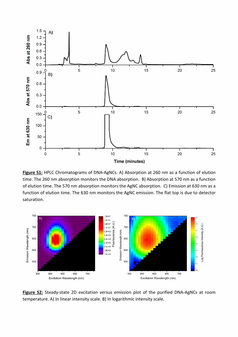
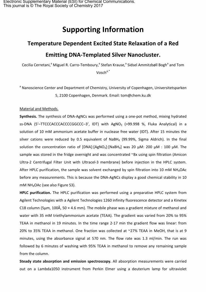
Figure S1: HPLC Chromatograms of DNA-AgNCs. A) Absorption at 260 nm as a function of elution time. The 260 nm absorption monitors the DNA absorption. B) Absorption at 570 nm as a function of elution time. The 570 nm absorption monitors the AgNC absorption. C) Emission at 630 nm as a function of elution time. The 630 nm monitors the AgNC emission. The flat top is due to detector saturation.

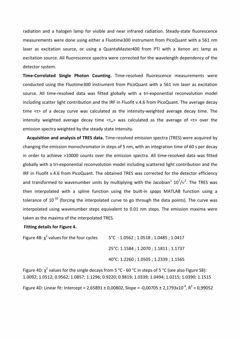
Figure S2: Steady-state 2D excitation versus emission plot of the purified DNA-AgNCs at room temperature. A) In linear intensity scale. B) In logarithmic intensity scale.

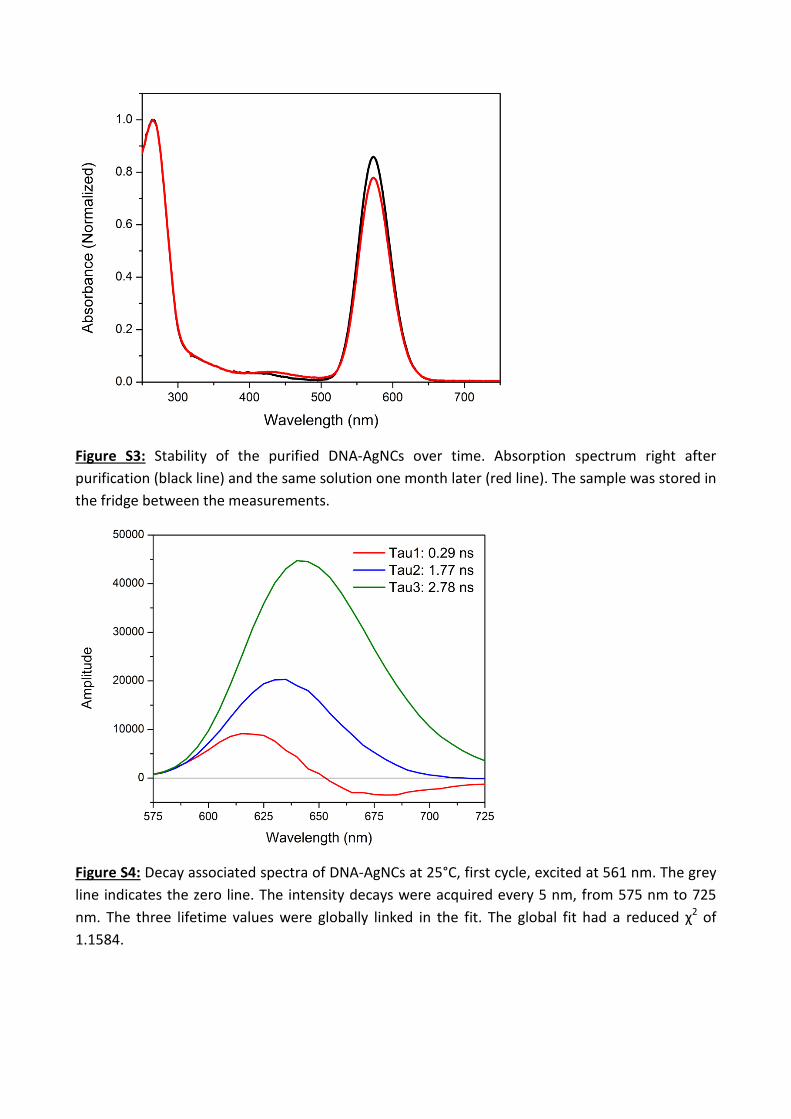
Figure S3: Stability of the purified DNA-AgNCs over time. Absorption spectrum right after purification (black line) and the same solution one month later (red line). The sample was stored in the fridge between the measurements.

Figure S4: Decay associated spectra of DNA-AgNCs at 25°C, first cycle, excited at 561 nm. The grey line indicates the zero line. The intensity decays were acquired every 5 nm, from 575 nm to 725 nm. The three lifetime values were globally linked in the fit. The global fit had a reduced χ2 of 1.1584.

Analysis of QY data and derivation of the QY equations.

The measured QY was plotted against the calculated <τω> for the measurements at different

temperatures (data from Cycle 1) and fitted with a linear model of the form (1)

QY(<τω>)=a<τω>-b

where a,b are positive constants (Fig. SQY). The variable <τω> was plotted against the temperature

T and fitted with a linear model of the form (2)

<τω>(T)=n-mT

where n,m are positive constants (Fig. SQY).

This implies that (3)

QY(T)=p-qT

where p=an-b and q=ma are positive constants. In this way we can relate all the constants of the

predictions derived from the linear regressions and use equations (2) and (3) to evaluate the

previous quantities in an extended temperature range. Note that this is a calculated extrapolation

and that parts of the extrapolation might not be physically realistic.

Fig. SQY A) Linear regression from measured data parameters a=0.77±0.05 ns-1 and b=1.2±0.1. B)

Linear regression from measured data used to extract the parameters m=0.0067±0.0005 ns°C-1

and n=2.74±0.01 ns.

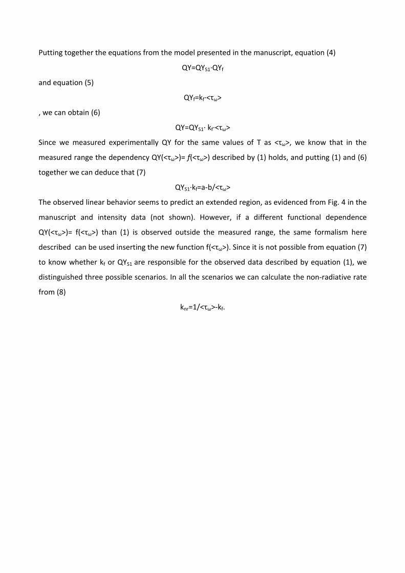
Putting together the equations from the model presented in the manuscript, equation (4)

QY=QYS1·QYf

and equation (5)

QYf=kf·<τω>

, we can obtain (6)

QY=QYS1· kf·<τω>

Since we measured experimentally QY for the same values of T as <τω>, we know that in the

measured range the dependency QY(<τω>)= f(<τω>) described by (1) holds, and putting (1) and (6)

together we can deduce that (7)

QYS1·kf=a-b/<τω>

The observed linear behavior seems to predict an extended region, as evidenced from Fig. 4 in the

manuscript and intensity data (not shown). However, if a different functional dependence

QY(<τω>)= f(<τω>) than (1) is observed outside the measured range, the same formalism here

described can be used inserting the new function f(<τω>). Since it is not possible from equation (7)

to know whether kf or QYS1 are responsible for the observed data described by equation (1), we

distinguished three possible scenarios. In all the scenarios we can calculate the non-radiative rate

from (8)

knr=1/<τω>-kf.

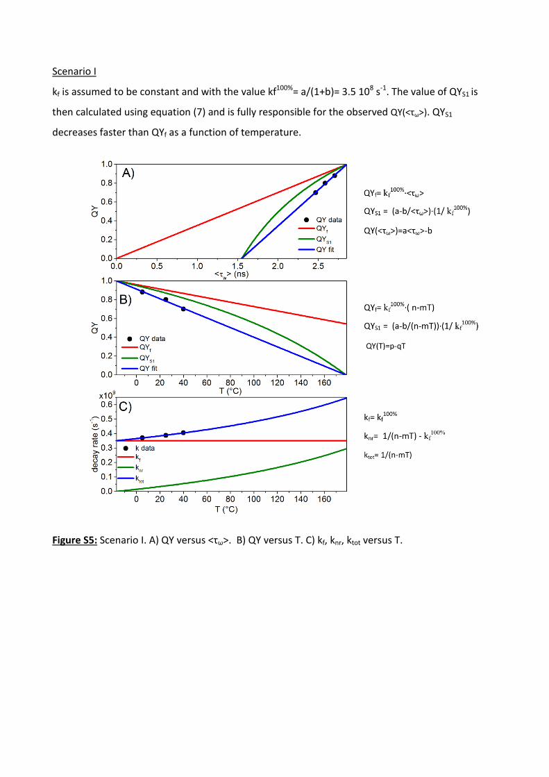
kf is assumed to be constant and with the value kf100%= a/(1+b)= 3.5 108 s-1. The value of QYS1 is

then calculated using equation (7) and is fully responsible for the observed QY(<τω>). QYS1

decreases faster than QYf as a function of temperature.

Scenario I

Figure S5:

Scenario I. A) QY versus <τω>. B) QY versus T. C) kf, knr, ktot versus T.

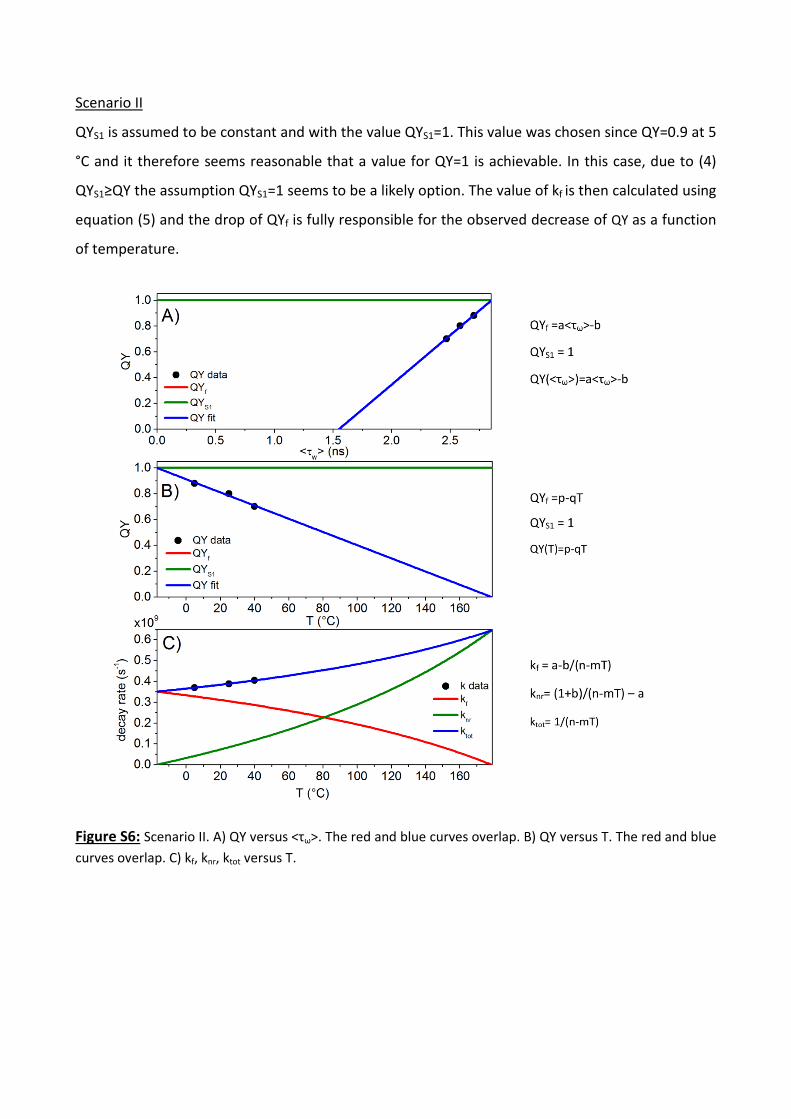
QYS1 is assumed to be constant and with the value QYS1=1. This value was chosen since QY=0.9 at 5

°C and it therefore seems reasonable that a value for QY=1 is achievable. In this case, due to (4)

QYS1≥QY the assumption QYS1=1 seems to be a likely option. The value of kf is then calculated using

equation (5) and the drop of QYf is fully responsible for the observed decrease of QY as a function

of temperature.

Scenario II

Figure S6: Scenario II. A) QY versus <τω>. The red and blue curves overlap. B) QY versus T. The red and blue curves overlap. C) kf, knr, ktot versus T.

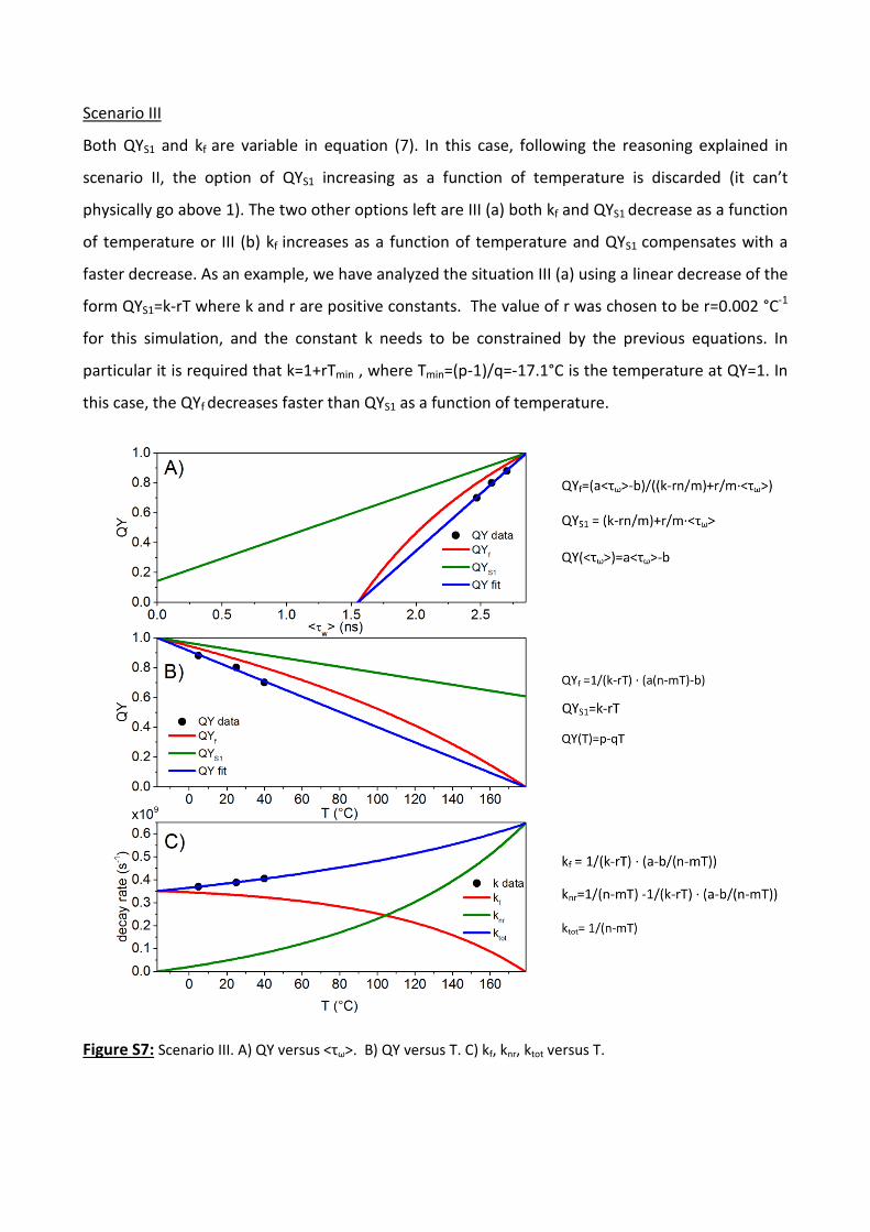
Both QYS1 and kf are variable in equation (7). In this case, following the reasoning explained in

scenario II, the option of QYS1 increasing as a function of temperature is discarded (it can’t

physically go above 1). The two other options left are III (a) both kf and QYS1 decrease as a function

of temperature or III (b) kf increases as a function of temperature and QYS1 compensates with a

faster decrease. As an example, we have analyzed the situation III (a) using a linear decrease of the

form QYS1=k-rT where k and r are positive constants. The value of r was chosen to be r=0.002 °C-1

for this simulation, and the constant k needs to be constrained by the previous equations. In

particular it is required that k=1+rTmin , where Tmin=(p-1)/q=-17.1°C is the temperature at QY=1. In

this case, the QYf decreases faster than QYS1 as a function of temperature.

Scenario III

Figure S7: Scenario III. A) QY versus <τω>. B) QY versus T. C) kf, knr, ktot versus T.

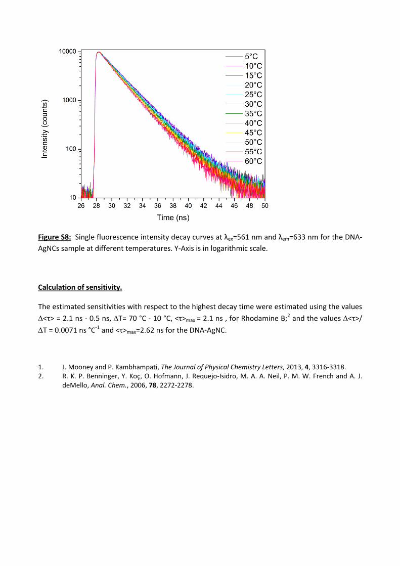
Figure S8: Single fluorescence intensity decay curves at λex=561 nm and λem=633 nm for the DNA-AgNCs sample at different temperatures. Y-Axis is in logarithmic scale.

Calculation of sensitivity.

The estimated sensitivities with respect to the highest decay time were estimated using the values ∆<τ> = 2.1 ns - 0.5 ns, ∆T= 70 °C - 10 °C, <τ>max = 2.1 ns , for Rhodamine B;2 and the values ∆<τ>/ ∆T = 0.0071 ns °C-1 and <τ>max=2.62 ns for the DNA-AgNC.

1. J. Mooney and P. Kambhampati, The Journal of Physical Chemistry Letters, 2013, 4, 3316-3318. 2. R. K. P. Benninger, Y. Koç, O. Hofmann, J. Requejo-Isidro, M. A. A. Neil, P. M. W. French and A. J.

deMello, Anal. Chem., 2006, 78, 2272-2278.