S-1

Supporting Information

Broadly Available Imaging Devices Enable High Quality Low-cost Photometry

Dionysios C. Christodouleas1, Alex Nemiroski1, Ashok A. Kumar1 and George M.

Whitesides1,2,3*

1 Department of Chemistry & Chemical Biology, Harvard University, 12 Oxford Street,

Cambridge, MA 02138, USA

2 Wyss Institute for Biologically Inspired Engineering, Harvard University, 60 Oxford Street,

Cambridge, MA 02138, USA

3 Kavli Institute for Bionano Science & Technology, Harvard University, 29 Oxford Street,

Cambridge, MA 02138, USA

*Corresponding author E-mail: gwhitesides@gmwgroup.harvard.edu

S-2

Experimental procedures

Construction of camera-based photometer. We first constructed a five-sided box from

cardboard and lined the inside with black fabric. A base formed by adhering a sheet of foam

(1” thick) underneath a perfboard provided a surface on which to solder components and fix them

in place. On to this perfboard, we soldered a series circuit consisting of two 9-V batteries

(connected electrically in parallel and in separate battery holders), a toggle switch, a potentiometer

(to adjust brightness), and a planar light source. We finally placed the box on the base and used a

biopsy punch to create a 6-mm hole in the lid of the box, centered on the planar light source, for

the camera. The imaging distance was 15.5 cm. A schematic of the camera-based photometer is

shown in Figure S-2. Although a larger backlight (e.g. from a tablet) could illuminate the whole

plate at once, the camera would have to be moved much farther away to reduce the angular spread

in optical path lengths through the samples.

Preparation of solutions of dyes. We prepared solutions of the dyes with the following

concentrations. Disperse orange 3 (2.81, 8.43, 14.05, 28.10, 42.15, 56.20 μΜ), methyl orange

(0.06, 0.24, 0.50, 1.00, 2.00, 4.00 μΜ), fluorescein (2.00, 4.00, 6.00, 8.00, 10.00, 16.00 μΜ),

DPPH (1.40, 2.81, 5.62, 8.43, 11.24, 16.86, 22.48, 28.10 μΜ), eosin Y (0.54, 1.00, 2.00, 2.69,

6.00, 8.00, 10.00, 13.45 μΜ), rhodamine B (0.16, 0.78, 1.17, 2.91, 3.92, 5.83, 8.74, 11.66 μΜ),

trypan blue (1.04, 2.08, 4.16, 6.24, 8.33, 10.41, 16.65, 20.82 μΜ), prussian blue (1.00, 2.00, 4.00,

6.00, 10.00, 14.04, 19.20 μΜ), malachite green (0.06, 0.24, 0.50, 1.00, 2.00, 4.00 μΜ),

methylene blue (1.00, 2.00, 4.00, 6.00, 8.00, 10.00, 15.70, 21.98 μΜ), chlorophyll b (1.1, 2.2,

4.4, 6.6, 8.8 μΜ).

S-3

Preparation of calibration lines of dyes. We added 400 μL of different solutions into

each well of a 96-well microtiter plate (we prepared one plate per dye) and read the absorbance

on a microplate spectrophotometer at the peak absorbance of these solutions (Table S-2). Then,

we captured the images of the microtiter plates contained these solutions using the flatbed

scanner and the camera-based photometer. We read the RGB values of three pixels (chosen at

random from within the image of each of the wells that contained these solutions) with Image J

or Microsoft Paint and recorded the mean values Ck of each group of RGB values. We

calculated the RGB-resolved absorbance Ak of each sample using Equation 3 of the main text

( and the guidelines for the selection of appropriate color value.

Concentration of solutions of dyes shown in Figure 2. Each row of the 96-well

microtiter plate contained 8 solutions of one of 11 different compounds, the four left columns at

the same, higher concentration and the four right columns at the same, lower concentration (see

Supporting Information for the concentration of the solutions : i) disperse orange 3 (Left: 70.2

μM / Right: 28.1 μM), ii) methyl orange (Left: 29.3 μM / Right: 14.6 μM), iii) fluorescein (Left:

20.0 μM / Right: 10.0 μM), iv) 2,2-diphenyl-1-picrylhydrazyl (DPPH; Left: 16.8 μM / Right: 8.4

μM), v) eosin Y (Left: 8.0 μM / Right: 4.0 μM), vi) rhodamine B (Left: 5.8 μM / Right: 1.4 μM),

vii) trypan blue (Left: 10.4 μM / Right: 6.2 μM), viii) prussian blue (Left: 19.2 μM / Right: 10.0

μM), ix) malachite green (Left: 6.0 μM / Right: 4.0 μM), x) methylene blue (Left: 10.0 μM /

Right: 4.0 μM), xi) chlorophyll b (Left: 8.8 μM / Right: 4.4 μM).

Analytical protocols of the six photometric assays. We summarize the type of assay

(e.g., ELISA, enzymatic assay) used for each test, and special characteristics of the absorbance

)(

)(

10log Bk

Sk

k CC

A

S-4

peaks that are used as an analytical signal in Table S-4. The absorbance spectra of the

chromogenic products of the assays are shown in Figure S-13. The analytical characteristics of

the calibration lines of the assays are shown in Figure S-6. The protocols we followed are the

following:

Lactate assay: We followed the “Instructions for Use” supplied with the Lactate Assay

Kit (BioVision). The kit contained all the necessary reagents (Lactate Assay Buffer, Lactate

Probe, Lactate Enzyme Mix and a 100 nmol/μL Lactic Acid Standard solution). We first

prepared solutions of lactate at different concentrations (40, 80, 120, 160, 200 μg/mL) to

construct a calibration curve. We then diluted the human serum samples (human serum

Innovative Research Inc ) 1:10 with Lactate Assay Buffer. We added 50 μL of standard or

sample per well and then added 50 μL of the Reaction Mix (consisting of 46:2:2 Lactate Assay

Buffer, Lactate Probe, Lactate Enzyme Mix). We covered the wells with a sealing tape and

incubated for 30 minutes in room temperature protected from light. Then, we read the

absorbance on a microplate spectrophotometer at a wavelength of 570 nm and captured an image

of the plate using the flatbed scanner in transmittance mode or the camera-based photometer.

Low-density lipoprotein (LDL) ELISA: We followed the “Instructions for Use” supplied

with the LDL Human ELISA Kit (Abcam). The kit included a 96-well plate, with LDL specific

antibodies immobilized onto each well, and all the necessary stock reagents (LDL standard,

biotinylated LDL, Streptavidin-Peroxidase Complex, Chromogen Substrate, Wash Buffer). We

first prepared working solutions of the necessary reagents. We then prepared solutions of LDL at

different concentrations (6.25, 25, 50, 100, 200 μg/mL) to construct a calibration curve. We also

dilute 1:50 the human serum samples (human serum Innovative Research Inc). We added 25 μL

of standard or sample per well and immediately added 25 μL of biotinylated LDL. We covered

S-5

the wells with a sealing tape and incubated for two hours at 37 ˚C. We then washed each well

five times with 200 μL of wash buffer manually. Then we added 50 μL of the Streptavidin-

Peroxidase Complex to each well and we incubated them for 30 minutes. We then washed each

well five times with 200 μL of wash buffer manually. We then added 50 μL of the Chromogen

Substrate (containing TMB) in each well and we incubated them for 12 minutes. Then we added

50 μL of Stop Solution to each well and immediately read the absorbance on a microplate

spectrophotometer at a wavelength of 450 nm and captured an image of the plate using the

flatbed scanner in transmittance mode or the camera-based photometer.

Anti-Treponema pallidum IgG Human ELISA: We followed the “Instructions for Use”

supplied with the Anti-Treponema pallidum IgG Human ELISA Kit (Abcam). The kit included a

96-well plate, with recombinant Treponema pallidum antigens immobilized onto each well, and

all the necessary stock reagents (IgG Sample Diluent, Stop Solution, Washing Solution,

Treponema pallidum anti-IgG HRP Conjugate, TMB Substrate Solution, Treponema pallidum

Positive Control, Treponema pallidum Cut-off Control, Treponema pallidum Negative Control).

We first prepared working solutions of the necessary reagents. We then dilute 1:10 the human

serum samples (VIROTROL® Syphilis Total Controls, human serum Innovative Research Inc).

We added 100 μL of controls or sample per well and covered the wells with a sealing tape and

incubated for one hours at 37 ˚C. We then washed each well three times with 300 μL of wash

buffer manually. Then we added 100 μL of the Treponema pallidum anti-IgG HRP Conjugate to

each well and we incubated them for 30 minutes. We then washed each well three times with 300

μL of wash buffer manually. We then added 100 μL of the TMB Substrate Solution in each well

and we incubated them for 15 minutes. Then we added 100 μL of Stop Solution to each well and

immediately read the absorbance on a microplate spectrophotometer at a wavelength of 450 nm

S-6

and captured an image of the plate using the flatbed scanner in transmittance mode or the

camera-based photometer.

Cyanomethemoglobin Assay: We followed the “Instructions for Use” supplied with the

Drabkin’s Reagent (Sigma Aldrich). We first prepared the Drabkin’s Solution by reconstituting

one vial of the Drabkin’s Reagent with 1000 mL of water, and adding 0.5 mL of a 30% Brij 35

solution. We then prepared a Cyanmethemoglobin Standard Solution containing 18 mg/mL of

human hemoglobin in Drabkin’s Solution. We prepared solutions of cyanmethemoglobin at

different concentrations (60, 80, 100, 120, 160, 180 mg/mL) to construct a calibration curve. We

also diluted 1:250 the blood samples (Meter Trax Control Level 1, Meter Trax Control Level 2

and Meter Trax Control Level 3) in Drabkin’s Solution and incubated for 15 minutes in room

temperature. We added 350 μL of the solutions per well and then we read the absorbance on a

microplate spectrophotometer at a wavelength of 540 nm and captured an image of the plate

using the flatbed scanner in transmittance mode or the camera-based photometer.

Bicinchoninic acid (BCA) assay: We followed the “Instructions” supplied with the

Micro BCA Protein Assay Kit (Thermo Scientific). We first prepared the Micro BCA Working

Reagent by mixing 25 parts of Micro BCA Reagent MA, 24 parts of Micro BCA Reagent MB

and 1 part of Micro BCA Reagent MC. We diluted the samples (antibodies raised in rabbit,

mouse or goat) 1:50 in Phosphate Buffer Saline, pH 7.4. We then prepared solutions of albumin

at different concentrations (1.0, 5.0, 10.0, 20.0, 40.0 μg/mL) to construct a calibration curve. We

added 150 μL of controls or sample and 150 μL of the Micro BCA Working Reagent in each

well and incubated for 2 hours at 37 ˚C. We then let the solutions to cool to room temperature

and we read the absorbance on a microplate spectrophotometer at a wavelength of 560 nm and

S-7

captured an image of the plate using the flatbed scanner in transmittance mode or the camera-

based photometer.

Griess Assay: We followed the “Instructions” supplied with the Griess Reagent (Sigma

Aldrich). We first prepared the Griess Solution by reconstituting Griess Reagent with 250 mL of

water. We then prepared solutions of nitrite ions at different concentrations (1.0, 7.0, 15.0, 30.0,

60.0 μΜ) to construct a calibration curve. We added 200 μL of controls or samples (tap or

bottled water) and 200 μL of the Griess Reagent in each well and incubated for 15 minutes in

room temperatures. We read the absorbance on a microplate spectrophotometer at a wavelength

of 540 nm and captured an image of the plate using the flatbed scanner in transmittance mode or

the camera-based photometer.

Calculation of RGB-resolved Absorbance using the flatbed scanner. We captured the

images of the microtiter plates contained the samples using the flatbed scanner in transmittance

mode. Using the software bundled with the scanner (Epson), we disabled all automatic correction

functions (Figure S1) and saved all images as Joint Photographic Experts Group (JPEG) files.

We next read the RGB values of three pixels (chosen at random from within the image of each of

the wells that contained solutions of the test compounds) with Image J or Microsoft Paint and

recorded the mean values Ck of each group of RGB values. We finally calculated the RGB-

resolved absorbance Ak of each sample using Equation 3 of the main text

and the guidelines for the selection of appropriate color value.

Calculation of RGB-resolved Absorbance using the camera-based photometer. The

planar light source used in the camera-based photometer was large enough to illuminate 32 wells

)(

)(

10log Bk

Sk

k CC

A

S-8

of a standard 96-microtiter plate, and therefore, we required three separate images (Figure S2A-

C) to capture an entire plate. We adjusted the settings on the camera of the cell-phone (LG

OPTIMUS F3 4G LTE) during image capture to the following: i) Focus: Auto, ii) ISO: 400, iii)

White balance: Auto, iv) Brightness: 0.0, v) Image size: 5M (2560×1920), vi) Color effect:

None. The cell-phone automatically saved images in the Joint Photographic Experts Group

(JPEG) format. After importing the images to a personal computer, we read the RGB values of

three pixels (chosen at random from within the image of each of the wells that contained

solutions of the test compounds) with Image J or Microsoft Paint and recorded the mean values

Ck of each group of RGB values.

To eliminate the influence of the slight spatial gradients in the intensity of light emitted

by the planar light source, we used the following procedure. For each assay, we first captured a

baseline image of 32 wells of a standard 96-microtiter plate filled with blank solutions and then

calculated )(BkC for each well. The relative standard deviation of the )(B

kC values of different

wells in this baseline measurement was ~2 % (N=32 wells). We next captured the sample image

of 32 wells filled with 28 samples and 4 blank solutions. To account for any changes in the white

balance from image to image (cell-phone cameras typically adjust white balance automatically),

we estimated a white balance correction factor W =mean Ck

(B, sample)éë

ùû / mean C

k

(B, baseline)éë

ùû, where

Ck

(B, sample) are the RGB values of the 4 blank solutions in the sample image and Ck

(B, baseline) are the

RGB values of the corresponding wells in the baseline image. We next corrected the color values

of the sample image by Ck

(S ) =WCk

(S , raw) . We finally calculated the RGB-resolved absorbance Ak

of each sample using these corrected values, Equation 3 of the main text ( ),

and the guidelines for the selection of appropriate color value.

)(

)(

10log Bk

Sk

k CC

A

S-9

Estimation of the spectral sensitivity S(λ) and the gamma correction factors γk for

RGB-based images sensors. Each individual pixel sensor of a RGB-based imaging device

employs a CCD or CMOS photodetector with a spectral responsivity R(λ), and red, green and

blue color filters, each with transmittance Fk (λ), where k = {R, G, B}. The total spectral

sensitivity of each pixel sensor is . Although we cannot measure these

individual contributions to Sk (λ) independently, we estimated this function by using an external

light source, a monochromator, and a fiber optic cable to deliver a pseudo delta-function inputs

to the pixel sensors such that , where λn is the central wavelength,

is the total intensity of the narrowband input with index (defined by the

monochromator). We determined the relationship between the measured color values and

sensitivity of each channel to be kk

nknkknnknk TSidSTiC

2

1, ,

where T accounts for all the losses between the monochromator and the RGB detector. Through

an independent measurement of in and with a fiber-coupled spectrophotometer, we estimated Sk

(up to unknown factors of γk, βk, and T) by Equation S-1.

(Eq. S-1)

Because is approximately continuous between the different that we measured, we used

Mathematica to interpolate the collected values and to form the

continuous function . Inspection of Equation 6 from the main text shows that the

unknown linear factors βk and T will drop out and therefore not contribute to the measurement of

absorbance.

Sk l( ) = R l( )Fk l( )

S-10

To calculate the values of γk for the RGB sensor, we first measured the RGB-resolved

absorbance values 𝐴𝑘(𝑚𝑒𝑎𝑠𝑢𝑟𝑒𝑑)for 11 different dyes at different concentrations. We then

calculated the expected RGB-resolved absorbance 𝐴𝑘(𝑒𝑥𝑝𝑒𝑐𝑡𝑒𝑑) by substituting the interpolated

function Sk(λ), given in Equation S-1, into Equation 6, and used the absorption spectra A(λ) of all

the dyes (measured on by a spectrophotometer) to calculate Ak for each color channel by

Equation S-2.

Ak = -g k logL l( )×10-AS (l ) ×

Ck l( )éë ùû1/gk

i l( )l1

l2

ò dl

L l( )×10-AB (l ) ×Ck l( )éë ùû

1/gk

i l( ) dl

l1

l2

ò

é

ë

êêêêê

ù

û

úúúúú

(Eq. S-2)

We plotted all the values of 𝐴𝑘(𝑚𝑒𝑎𝑠𝑢𝑟𝑒𝑑) vs 𝐴𝑘

(𝑒𝑥𝑝𝑒𝑐𝑡𝑒𝑑), and used γk as a single free parameter fit

the data to unity slope (within± 0.001), shown in Figure S-12. Using this approach, we

determined γk for the scanner to be γR = 0.617, γG = 0.472, γB = 0.498, and γk for the camera to be

γR = 0.724, γG = 0.525, γB = 0.778.

Definition of Standard and Peak Absorbance. The spectral intensity of light that

is transmitted by an arbitrary sample is , where is the spectral intensity

of the light source and is the absorbance of the sample at any given wavelength λ. The

transmittance of the sample, relative to free space, therefore, is and

. In general, (known as the Beer-Lambert law),

where is the molar extinction coefficient of the sample, d is the optical path length through

the sample, and c is the concentration of the sample, and is the absorption of the

I l( )

I l( ) = I0 l( )10-A l( )I0 l( )

A l( )

T l( ) = I l( ) / I0 l( ) =10-A l( )

A l( ) = - logT l( ) A l( ) =e l( )×d×c+Ab l( )

e l( )

Ab l( )

S-11

background (or blank). To eliminate the contribution of the background absorption of the

solution (not related to the concentration of the sample), the absorbance is typically defined

relative to a blank solution, as shown in Equation S-3.

(Eq. S-3)

The peak absorbance Apeak occurs at the wavelength λpeak where A is a maximum, and is also

linearly related to c. After calibrating a system with standard concentrations of a known dye,

measuring Apeak enables a highly sensitive determination of an unknown concentration c of the

known dye. This measurement is the standard method of determining the absorbance of a sample

and requires sophisticated equipment (a spectrophotometer) that incorporates a monochromator

or a narrowband filter to isolate the bandwidth of the measurement narrowly around λpeak, and to

tune the value of λpeak to match spectral characteristics the compound being tested.

The narrowband absorbance defined by Eq. S-3 is a special case of the more generalized

broadband absorbance defined by Equation 4 in the main text. The spectral distribution of a

spectrophotometer is controlled by a diffraction grating that disperses the light so that each

element of the photodetector array only receives a very narrow band of wavelengths. We can

approximate this behavior by replacing the broadband spectral sensitivity by a delta-like function

such that 𝑆𝑘(𝜆) → 𝑆𝑘(𝜆)𝛿(𝜆 − 𝜆0), where λ0 is the central wavelength of the light diffracted to

each pixel. Assuming that γk = 1 for the photodetector array, Equation 4 of the main text reduces

to Eq. S-4.

A = As l( )- Ab l( ) = - logIs l( )Ib l( )

é

ëêê

ù

ûúú= e l( )×d ×c

)()(1010log

)(10

)(10log 00

0)(

0

0)(

010

0)(

0)(

0

0

2

1

2

1

BSA

A

A

A

AASLSL

dSL

dSLA

B

S

B

S

(Eq. S-4)

S-12

Choice of RGB color system rather than grayscale or HSV. Although we are free to

explore any of the available methods for representing color intensity, we chose to use the R, G,

or B values because: i) most digital imaging devices use the RGB color system to digitize the

image; ii) RGB values of the pixels of an image are easily read using commonly available

software (e.g. Microsoft Paint, Adobe Illustrator, Image J); iii) RGB values can be considered as

metrics of the total light intensity within certain bandwidths corresponding to the light that

passes through the red, green and blue filters that are present on the surface of the CCD/CMOS

photodetector. The intensity of the gray scale value (x) and the hue (H) component of hue-

saturation-value (HSV) color system are other parameters that have been used in the past to

correlate the color of the sample with the concentration of an analyte.13 These values are simply

linear (gray scale) or nonlinear (hue) combinations of the recorded RGB values, and are defined

by Equation S-5 and Equation S-6.

x = 0.299R + 0.587G + 0.114B, (Eq. S-5)

(Eq. S-6)

Spectral peaks, however, typically overlap most strongly with only one RGB color channel.

Combining these RGB values into grayscale or HSV values, therefore, adds information about

light intensity that is not related to the concentration of the sample, and consequently, makes

these color values less sensitive to changes in concentration than the raw RGB values.

GBifGBRBRGBGR

BGR

BGifGBRBRGBGR

BGR

H

,cos360

,cos

222

1

222

1

S-13

Figure S-1. Screenshots of the control window of the software of the scanner

S-14

Figure S-2. Schematic of the camera-based photometer

S-15

Figure S-3. A-C) Images of a standard microtiter plate containing solutions of 11 chromogenic

dyes inside the camera-based photometer. D) Image of the camera-based photometer

disassembled, including a cell-phone, a microtiter plate containing colored dyes, a folded

cardboard box, and the base.

A

B

C

D

S-16

Figure S-4. An image of a microtiter plate, containing solutions of 11 dyes (one per row;

lowest/twelfth row contains an aqueous blank) in two concentrations (four left columns vs. four

right columns) captured by the CIS scanner in reflectance mode

S-17

Figure S-5. A) Absorbance spectra of disperse orange 3 in ethanolic solution (7.0 μΜ), methyl

orange in aqueous solution (29.3 μΜ), and fluorescein in aqueous solution (20.0 μΜ). B)

Absorbance spectra of DPPH in methanolic solution (16.8 μΜ), eosin Y in aqueous solution

(8.0 μΜ), and rhodamine B in aqueous solution (5.8 μΜ). C) Absorbance spectra of trypan blue

in aqueous solution (10.0 μΜ), prussian blue in aqueous solution (19.2 μΜ), malachine green in

aqueous solution (6.0 μΜ), methylene blue in aqueous solution (10.0 μΜ), and chlorophyll b in

aqueous solution (8.8 μΜ).

A

B

C

S-18

Figure S-6. A screenshot that shows how to use Image J to read the RGB color value of a well

containing a solution. The RGB values are outlined by the red box.

S-19

Figure S-7. A screenshot that shows how to use Microsoft Paint to read the RGB color value of a

well containing a solution. The necessary steps prior to the reading are indicated: 1) choose eye-

dropper tool and select a pixel, 2) select Colors, 3) select Edit Colors, 4) select Define Custom

Colors. Finally, read out the RGB values (outlined by the red box).

S-20

Figure S-8. i) Characterization of the spectrum of the light emitted from the light source of the

flatbed scanner (A) or the planar light source (E). ii) Transmittance spectra of a 10-μΜ

methylene blue solution (sample) and DI water (blank) measured in the microplate

spectrophotometer (B, F). iii) Spectral sensitivity, Sk(λ), of the image sensor of the scanner (C)

and the cell-phone camera (G). iv) The light intensity that reach the CCD/CMOS detector of the

flatbed scanner (D) and the cell-phone camera (H) during the imaging of a 10 μΜ methylene

blue solution (sample) and DI water (blank).

A E

B F

C G

D H

S-21

Figure S-9. Absorbance spectra of the chromogenic products of the following six assays: A)

Lactate assay (lactic acid, 160 μg/mL), B) LDL / Anti-Treponema pallidum Ig ELISAs (blank

solution / cut-off control), C) BCA assay (albumin, 40.0 μg/mL), D) Cyanomethemoglobin assay

(hemoglobin, 160 mg/mL), E) Griess assay (nitrite ions, 60.0 μΜ)

A C B

D E

S-22

Figure S-10. Histograms of green channel of an image of a well (inset) containing a 6.00 μM

Eosin Y solution captured using the flatbed scanner in (A) transmittance mode, (B) reflectance

mode, and (C) a scanner (using CSI technology) in reflectance mode. D) Table containing the

characteristics of the distributions.

A

B

C

D

S-23

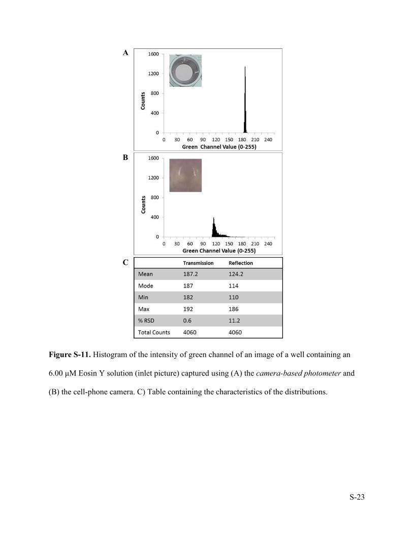
Figure S-11. Histogram of the intensity of green channel of an image of a well containing an

6.00 μM Eosin Y solution (inlet picture) captured using (A) the camera-based photometer and

(B) the cell-phone camera. C) Table containing the characteristics of the distributions.

A

B

C

S-24

Figure S-12. Correlation plots of measured RGB-resolved Absorbance Values of solutions of 11

dyes measured using the scanner (A-C) and the camera-based photometer (D–F) vs the expected

RGB-resolved absorbance values calculated using Equation S-2. Each of plots only show results

from the solutions that absorb most strongly within the bandwidth of the labeled color channel:

plots (A, D) show measurements from solutions of disperse orange 3, methyl orange and

fluorescein; plots (B, E) show measurements from solutions of DPPH, eosin Y and rhodamine B;

plots (C, F) show measurements from solutions of disperse orange 3, methyl orange and

fluorescein.

A

B

C

D

E

F

S-25

Figure S-13. Correlation plots of peak absorbance values (Apeak) of three chromogenic

compounds (methylene blue, DPPH, and methyl orange), which absorb in a different color

channel, measured using the microplate spectrophotometer vs RGB-resolved absorbance values

measured using the flatbed scanner (A) or the camera-based photometer (B). Each data point

corresponds to the mean value of seven measurements

A

B

S-26

Table S-1. Comparison of the analytical characteristics of correlation lines* fitted to the peak

absorbance values (Apeak, measured by the microplate spectrophotometer as the laboratory

standard) vs. the RGB-resolved absorbance values (Ak, measured by flatbed scanner or the

camera-based photometer) for solutions of 11 different dyes.

Compound λmax

†

/ Color channel‡

Peak absorbance vs RGB-resolved absorbance (flatbed scanner)

Peak absorbance vs RGB-resolved absorbance (camera-based

photometer)

Intercept Slope Correlation coefficient Intercept Slope Correlation

coefficient

a×10-3 (±sa)

b×10-3 (±sb)

R a×10-3 (±sa)

b×10-3 (±sb)

R

Disperse orange 3

440 nm /Blue

0.0018 2.2002 0.99998

0.024 1.28 0.99 (± 0.0009) (± 0.0054) (± 0.018) (± 0.10)

Methyl orange

465 nm /Blue

-0.0109 2.346 0.9997 0.037 1.24 0.999 (± 0.0052) (± 0.023) (± 0.026) (± 0.11)

Fluorescein 485 nm /Blue

-0.0283 2.93 0.997 0.0126 2.181 0.997 (± 0.0091) (± 0.12) (± 0.0069) (± 0.076)

DPPH 515 nm /Green

-0.0086 3.085 0.9999 0.044 2.286 0.995 (± 0.0028) (± 0.017) (± 0.020) (± 0.096)

Eosin Y 518 nm /Green

-0.052 16.17 0.996 -0.067 16.51 0.99 (± 0.018) (± 0.60) (± 0.029) (± 0.96)

Rhodamine B

555 nm /Green

-0.026 4.43 0.997 -0.005 5.51 0.997 (± 0.016) (± 0.14) (± 0.015) (± 0.16)

Trypan blue 585 nm /Red

-0.027 3.207 0.998 0.050 2.27 0.99 (± 0.013) (± 0.086) (± 0.026) (± 0.18)

Prussian Blue

605 nm /Red

-0.017 2.635 0.998 0.065 1.316 0.99 (± 0.011) (± 0.069) (± 0.027) (± 0.097)

Malachine green

618 nm /Red

-0.0057 2.884 0.9993 -0.05 2.61 0.99 (± 0.0071) (± 0.050) (± 0.05) (± 0.21)

Methylene blue

662 nm /Red

0.0100 3.532 0.99997 0.010 1.756 0.996 (± 0.0019) (± 0.011) (± 0.015) (± 0.072)

Chlorophyll b

462 nm /Red

-0.0097 2.624 0.9996 0.033 1.40 0.99 (± 0.0050) (± 0.030) (± 0.021) (± 0.11)

*All absorbance values were estimated by the mean value of N = 7 measurements. The regression

equation we used was: A = a + b× Ak.

† The spectral bandwidth is ± 5 nm

‡ The RGB color channel value used for the estimation of the RGB-resolved absorbance values of the

tested solutions

S-27

Table S-2. Comparison of the analytical characteristics of calibration lines† fitted to the peak

absorbance values (Apeak, measured by the microplate spectrophotometer as the laboratory

standard) and the RGB-resolved absorbance values (Ak, measured by flatbed scanner or the

camera-based photometer) vs. concentration of analyte (measured in μM) for solutions of 11

different dyes.

†All absorbance values were estimated by the mean value of N = 7 measurements. The regression

equation we used was: A = a + b× Ak

* The spectral bandwidth is ± 5 nm

*** The RGB color channel value used for the estimation of the RGB-resolved absorbance values of the

tested solutions

S-28

Table S-3. Comparison of the results for the spectrophotometer (laboratory standard) vs. the

flatbed scanner and camera-based photometer in the following six analyses: i) Lactate assay, ii)

LDL ELISA, iii)Anti-Treponema pallidum IgG assay, iv) BCA assay, v) Cyanomethemoglobin

assay, and vi) Griess assay. The values and error bars correspond to the mean and standard

deviations, respectively, of N = 7 measurements. The Anti-Treponema pallidum ELISA only

permits qualitative results. The concentration of nitrite ions in the third sample tested with the

Griess assay was lower than the detection limit of the method and therefore labeled as “Not

Determined” (N.D.).

Assay

λmax†/ Color

Channel‡ Sample

Microplate

spectrophotometer Flatbed Scanner

Camera-based

photometer

Concentration (± SD)

Lactate 570 nm /Green

Serum 1 3.280 ± 0.064 mΜ 3.284 ± 0.042 mΜ 3.223 ± 0.105 mΜ Serum 2 1.078 ± 0.027 mΜ 1.072 ± 0.016 mΜ 1.084 ± 0.037 mΜ Serum 3 2.575 ± 0.052 mΜ 2.594 ± 0.017 mΜ 2.634 ± 0.071 mΜ

LDL ELISA 450 nm /Blue

Sample 1 3.76 ± 0.17 mg/mL 3.75 ± 0.12 mg/mL 3.74 ± 0.17 mg/mL Sample 2 2.35 ± 0.11 mg/mL 2.39 ± 0.12 mg/mL 2.42 ± 0.21 mg/mL Sample 3 4.59 ± 0.31 mg/mL 4.50 ± 0.23 mg/mL 4.61 ± 0.35 mg/mL

Anti-Treponema

pallidum IgG ELISA

450 nm /Blue

Serum 1 positive positive positive Serum 2 positive positive positive

Serum 3 negative negative negative

Bicinchoninic acid (BCA)

560 nm /Green

Sample 1 1.749± 0.026 mg/mL 1.755 ± 0.013 mg/mL 1.716 ± 0.080 mg/mL Sample 2 1.934 ± 0.034 mg/mL 1.890 ± 0.051 mg/mL 1.965 ± 0.084 mg/mL Sample 3 2.999 ± 0.045 mg/mL 2.977 ± 0.041 mg/mL 3.070 ± 0.081 mg/mL

Cyanmethemo-globin

540 nm /Green

Blood 1 94.1± 2.1 mg/mL 93.2 ± 1.4 mg/mL 91.2 ± 5.0 mg/mL Blood 2 175.6 ± 2.8 mg/mL 173.1 ± 2.1 mg/mL 172.3 ± 4.4 mg/mL Blood 3 179.1 ± 1.8 mg/mL 177.1 ± 1.8 mg/mL 177.2 ± 4.3 mg/mL

Griess 540 nm /Green

Water 1 35.90 ± 0.21 mΜ 35.94 ± 0.45 mΜ 34.99 ± 0.99 mΜ Water 2 2.87 ± 0.20 mΜ 2.78 ± 0.10 mΜ 2.92 ± 0.76 mΜ Water 3 ND ND ND

* All absorbance values were estimated by the mean value of N = 7 measurements.

† The spectral bandwidth is ± 5 nm

‡ The RGB color channel value used for the estimation of the RGB-resolved absorbance values of the

tested solutions.

S-29

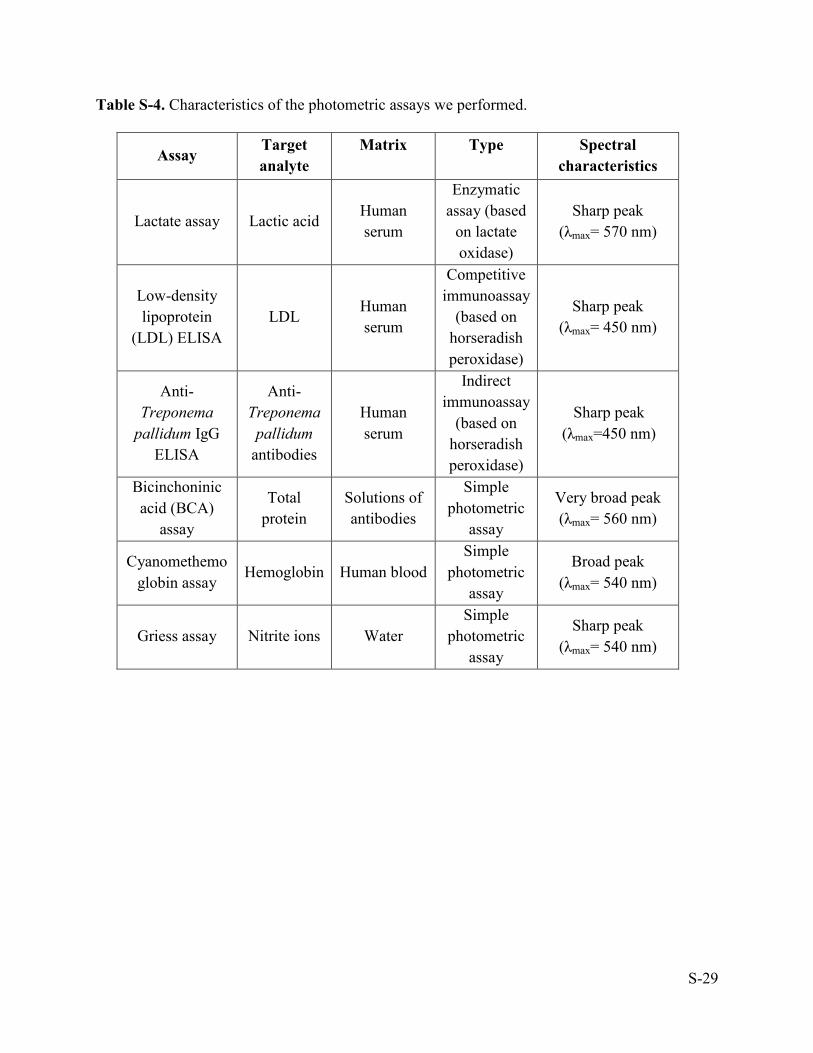
Table S-4. Characteristics of the photometric assays we performed.

Assay Target analyte

Matrix

Type

Spectral characteristics

Lactate assay Lactic acid Human serum

Enzymatic assay (based

on lactate oxidase)

Sharp peak (λmax= 570 nm)

Low-density lipoprotein

(LDL) ELISA LDL

Human serum

Competitive immunoassay

(based on horseradish peroxidase)

Sharp peak (λmax= 450 nm)

Anti-Treponema

pallidum IgG ELISA

Anti-

Treponema pallidum

antibodies

Human serum

Indirect immunoassay

(based on horseradish peroxidase)

Sharp peak (λmax=450 nm)

Bicinchoninic acid (BCA)

assay

Total protein

Solutions of antibodies

Simple photometric

assay

Very broad peak (λmax= 560 nm)

Cyanomethemoglobin assay

Hemoglobin Human blood Simple

photometric assay

Broad peak (λmax= 540 nm)

Griess assay Nitrite ions Water Simple

photometric assay

Sharp peak (λmax= 540 nm)

S-30

Table S-5. Analytical characteristics of calibration lines* for the following five assays: a) Lactate

assay, b) LDL ELISA, c) BCA assay, d) Cyanomethemoglobin assay, and e) Griess assay

Assay λmax† /Color

Channel‡

Microplate

spectrophotometer Flatbed scanner Camera-based photometer Intercept Slope

R2

Intercept Slope R

2

Intercept Slope R

2 a×10

-3

(±sa)

b×10-3

(±s

b)

a×10-3

(±s

a)

b×10-3

(±s

b)

a×10-3

(±s

a)

b×10-3

(±s

b)

Lactate assay (μΜ lactic acid)

570 nm /Green

19.3 4.991 0.9999 18.2 1.39 0.998

-3.75 1.49 0.998 (± 3.1) (± 0.023) (± 4.1) (± 0.031) (± 4.8) (± 0.036) LDL ELISA

(μg/mL LDL) 450 nm /Blue

606 -234 0.99 244 -101 0.992

331 -135 0.95 (± 48) (± 25) (± 10) (± 6.4) (± 35) (± 21) Cyanomethe-

moglobin Assay (mg/mL hemoglobin)

540 nm /Green

1.9 1.797 0.9995

1.9 0.698 0.998

-4.1 0.735 0.998

(± 2.5) (± 0.020) (± 1.5) (± 0.012) (± 1.7) (±0.013)

BCA assay (μg/mL albumin)

560 nm /Green

-1.3 12.07 0.999 0.1 4.819

0.9993 0.1 4.79

0.997 (± 4.7) (± 0.22) (± 1.5) (± 0.073) (± 3.4) (± 0.16) Griess Assay

(μM nitrite ions) 540 nm /Green

-4.3 15.84 0.9999 5.2 5.47

0.999 -3.9 6.00

0.997 (± 1.6) (± 0.05) (± 3.5) (± 0.11) (± 5.6) (± 0.17)