support vector machines h. clara pong julie horrocks 1, marianne van den heuvel 2,francis tekpetey...
Post on 18-Dec-2015
212 views
TRANSCRIPT
Support Vector MachinesSupport Vector MachinesH. Clara PongH. Clara Pong
Julie HorrocksJulie Horrocks11, Marianne Van den Heuvel, Marianne Van den Heuvel22,Francis Tekpetey,Francis Tekpetey3,3, B. Anne Croy B. Anne Croy4.4.
1 Mathematics & Statistics, University of Guelph, 1 Mathematics & Statistics, University of Guelph, 2 Biomedical Sciences, University of Guelph, 2 Biomedical Sciences, University of Guelph, 3 Obstetrics and Gynecology, University of Western Ontario, 3 Obstetrics and Gynecology, University of Western Ontario, 4 Anatomy & Cell Biology, Queen’s University4 Anatomy & Cell Biology, Queen’s University
OutlineOutline
BackgroundBackground Separating Hyper-plane & Basis Expansion Separating Hyper-plane & Basis Expansion Support Vector MachinesSupport Vector Machines SimulationsSimulations RemarksRemarks
BackgroundBackground
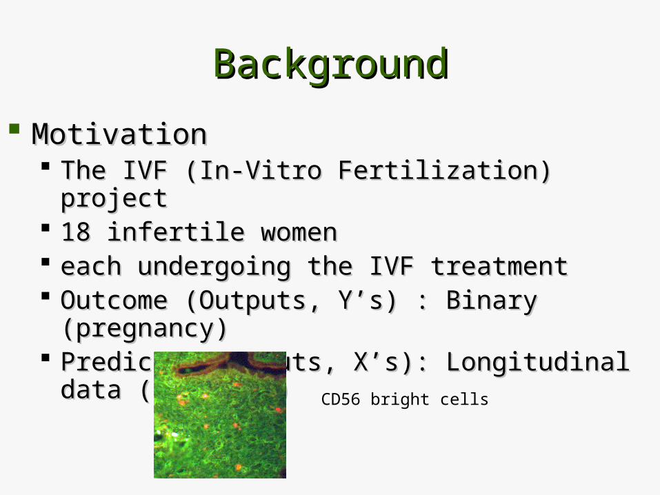
MotivationMotivation The IVF (In-Vitro Fertilization) project The IVF (In-Vitro Fertilization) project 18 infertile women 18 infertile women each undergoing the IVF treatment each undergoing the IVF treatment Outcome (Outputs, Y’s) : Binary (pregnancy)Outcome (Outputs, Y’s) : Binary (pregnancy) Predictor (Inputs, X’s): Longitudinal data (adhesion)Predictor (Inputs, X’s): Longitudinal data (adhesion)
CD56 bright cells
BackgroundBackground
Classification methods methods Relatively new method: Relatively new method: Support Vector MachinesSupport Vector Machines
- V. Vapnik: first proposed in 1979
- Maps input space into a high dimensional feature space input space into a high dimensional feature space
- Constructs a linear classifier in the new feature space feature space
Traditional method:Traditional method: Discriminant Analysis Discriminant Analysis- R.A. Fisher:R.A. Fisher: 1936
- Classify according to the values from the discriminant functions
- Assumption: the predictors X in a given class has a Multi-Normal distribution.
Separating Hyper-planeSeparating Hyper-plane
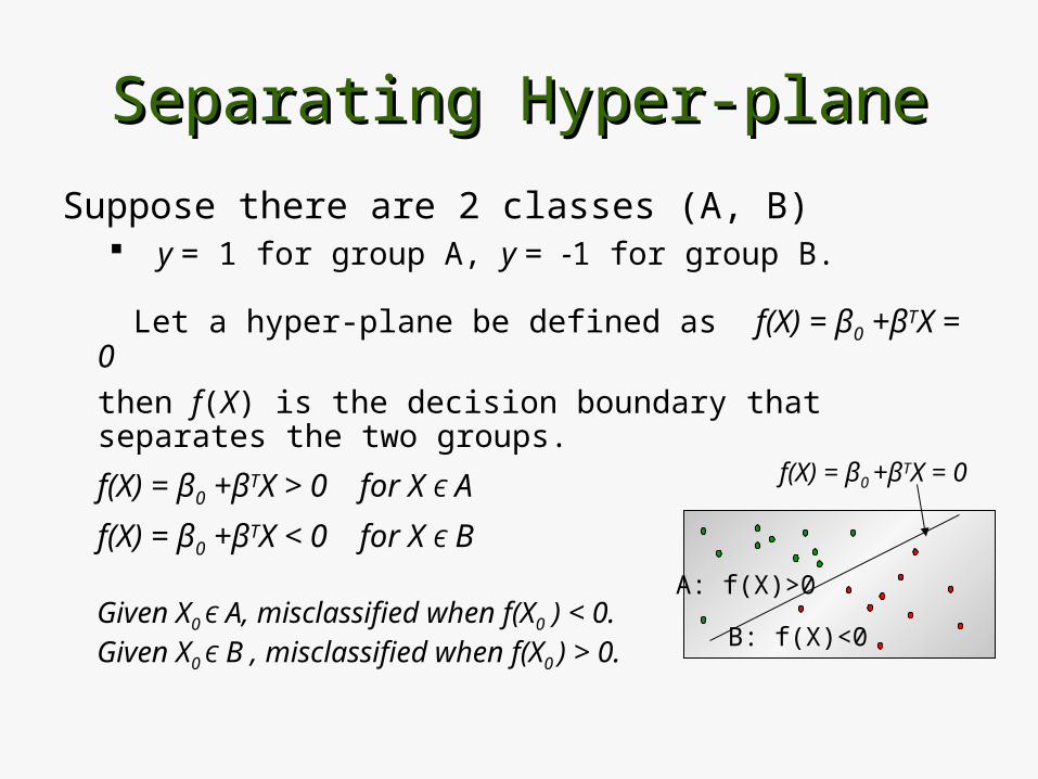
Suppose there are 2 classes (A, B) y = 1 for group A, y = -1 for group B.
Let a hyper-plane be defined as f(X) = β0 +βTX = 0
then f(X) is the decision boundary that separates the two groups.
f(X) = β0 +βTX > 0 for X Є A
f(X) = β0 +βTX < 0 for X Є B
Given X0 Є A, misclassified when f(X0 ) < 0.Given X0 Є B , misclassified when f(X0 ) > 0.
f(X) = β0 +βTX = 0
A: f(X)>0
B: f(X)<0
f(X) = β 0 +βT X = 0
Separating Hyper-planeSeparating Hyper-plane
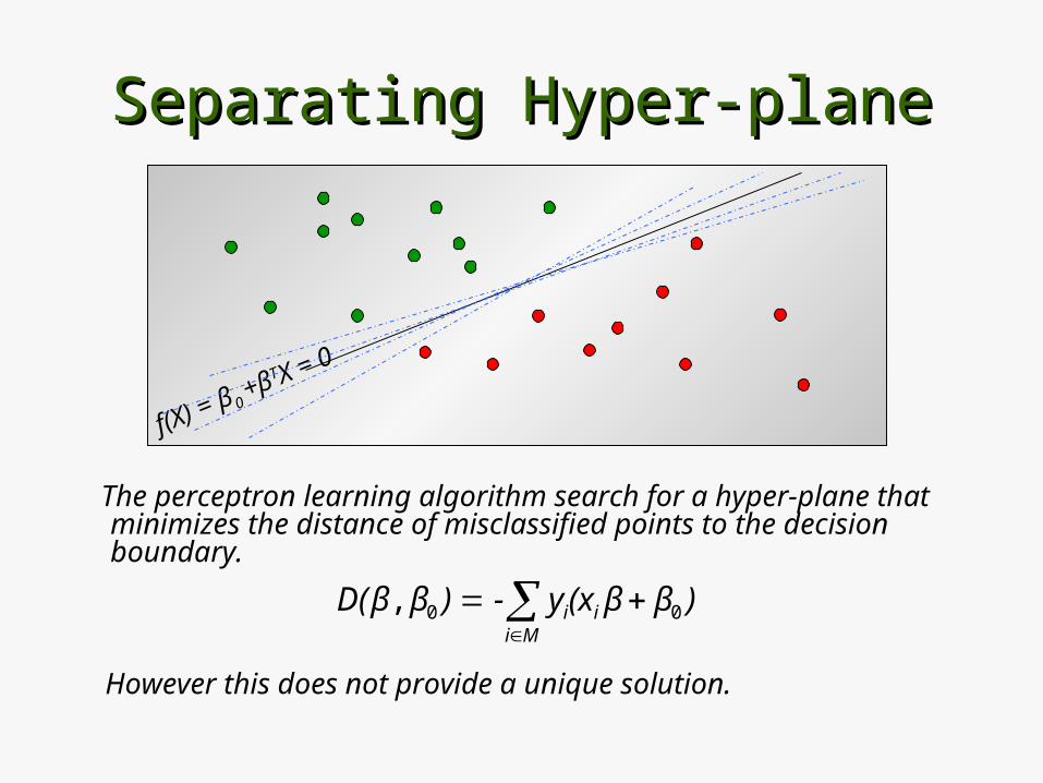
The perceptron learning algorithm search for a hyper-plane that minimizes the distance of misclassified points to the decision boundary.
However this does not provide a unique solution.
Mi
ii )ββ(xy -) βD(β 00,
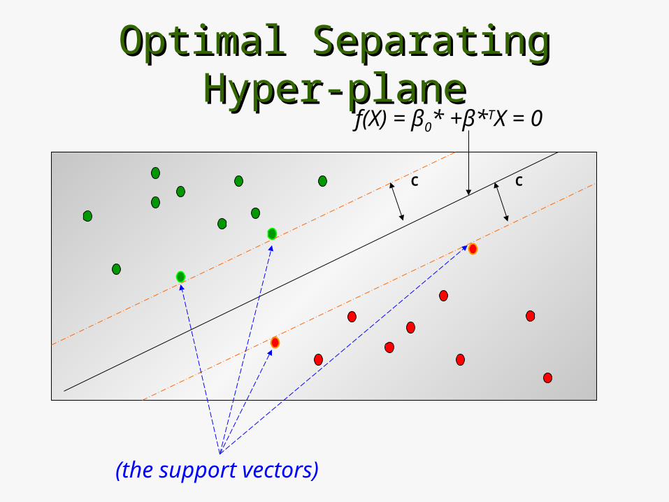
Optimal Separating Hyper-planeOptimal Separating Hyper-plane
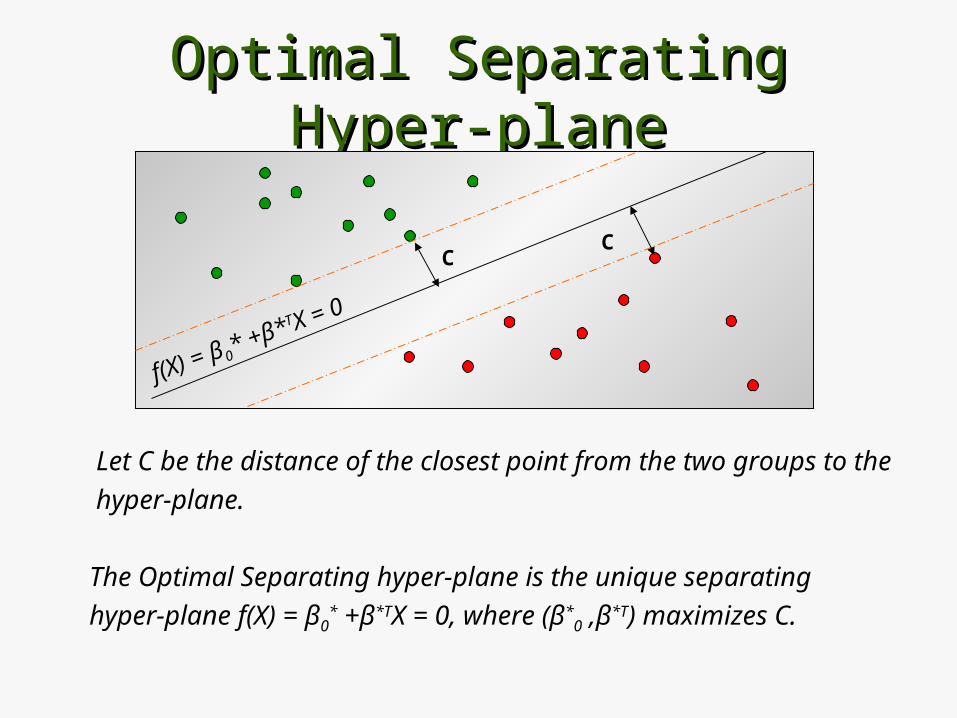
Let C be the distance of the closest point from the two groups to the
hyper-plane.
The Optimal Separating hyper-plane is the unique separating
hyper-plane f(X) = β0* +β*TX = 0, where (β*
0 ,β*T) maximizes C.
f(X) = β0* +β*TX = 0
CC
Optimal Separating Hyper-planeOptimal Separating Hyper-plane
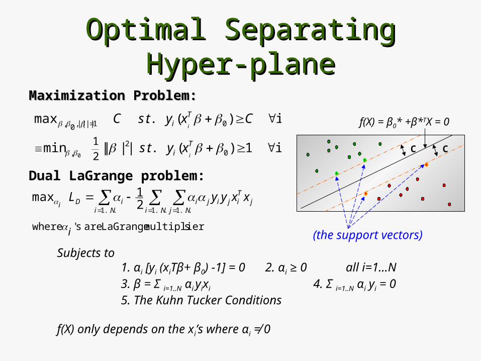
Maximization Problem:Maximization Problem:
C
f(X) = β0* +β*TX = 0
C
(the support vectors)
i 1)( .. ||||min
i )( .. max
02
,
01||||,0,
21
0
Ti
Ti
i
i
xyts
CxytsC
smultiplier LaGrange are s' where
21 max
...1 ...1...1
i
Nij
Tiji
Njji
NiiDi
xxyyL
Dual LaGrange problem:
Subjects to 1. αi [yi (xiTβ+ β0) -1] = 0 2. αi ≥ 0 all i=1…N 3. β = Σ i=1..N αi yixi 4. Σ i=1..N αi yi = 0 5. The Kuhn Tucker Conditions
f(X) only depends on the xi’s where αi ≠ 0
Optimal Separating Hyper-planeOptimal Separating Hyper-plane
C
f(X) = β0* +β*TX = 0
C
(the support vectors)
Basis ExpansionBasis Expansion
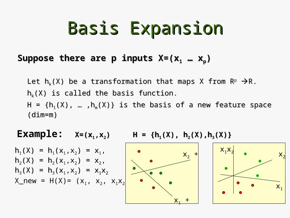
Suppose there are p inputs X=(xSuppose there are p inputs X=(x1 … x … xpp))
Let hLet hkk(X) be a transformation that maps X from R(X) be a transformation that maps X from Rp R.R.
hhkk(X) is called the basis function.(X) is called the basis function.
H = {hH = {h11(X), … ,h(X), … ,hmm(X)} is the basis of a new feature space (dim=m)(X)} is the basis of a new feature space (dim=m)
Example: X=(xX=(x1,x2)) H = {hH = {h1(X), h(X), h2(X),h(X),h3(X)}(X)}
hh1(X) = h(X) = h1(x(x1,x2) = x) = x1,
hh2(X) = h(X) = h2(x(x1,x2) =) = xx2,
hh3(X) = h(X) = h3(x(x1,x2) =) = xx11xx22
X_new = H(X)= (x1, x2, x1x2) x1
x2
x1x2
x1 +
x2 +
Support Vector MachinesSupport Vector Machines
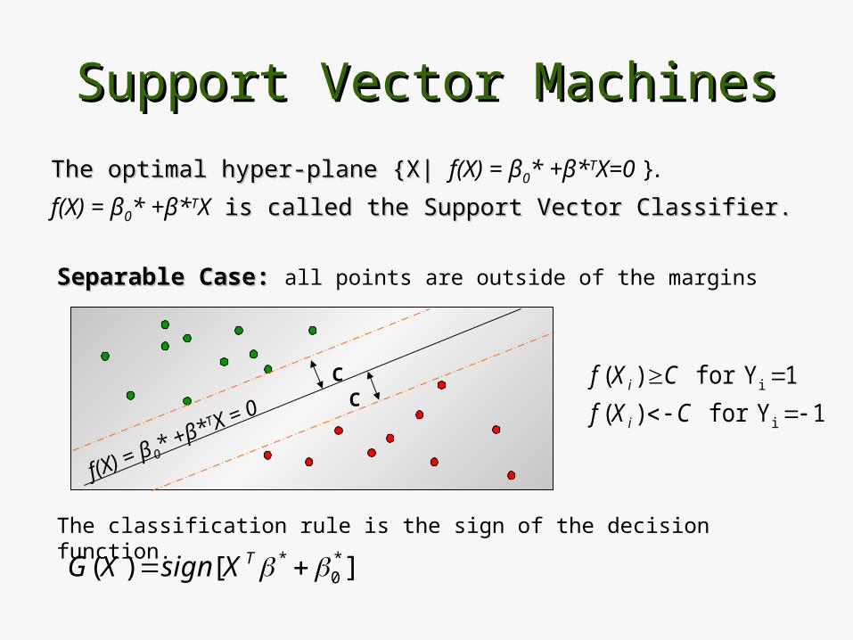
The optimal hyper-plane {X| The optimal hyper-plane {X| f(X) = β0* +β*TX=0 }.
f(X) = β0* +β*TX is called the Support Vector Classifier. is called the Support Vector Classifier.
Separable Case:Separable Case: all points are outside of the margins
The classification rule is the sign of the decision function.
][ )( *0
* TXsignXG
1Yfor )(
1Yfor )(
i
i
CXf
CXf
i
i
f(X) = β 0* +β*TX = 0
CC
Support Vector MachinesSupport Vector Machines
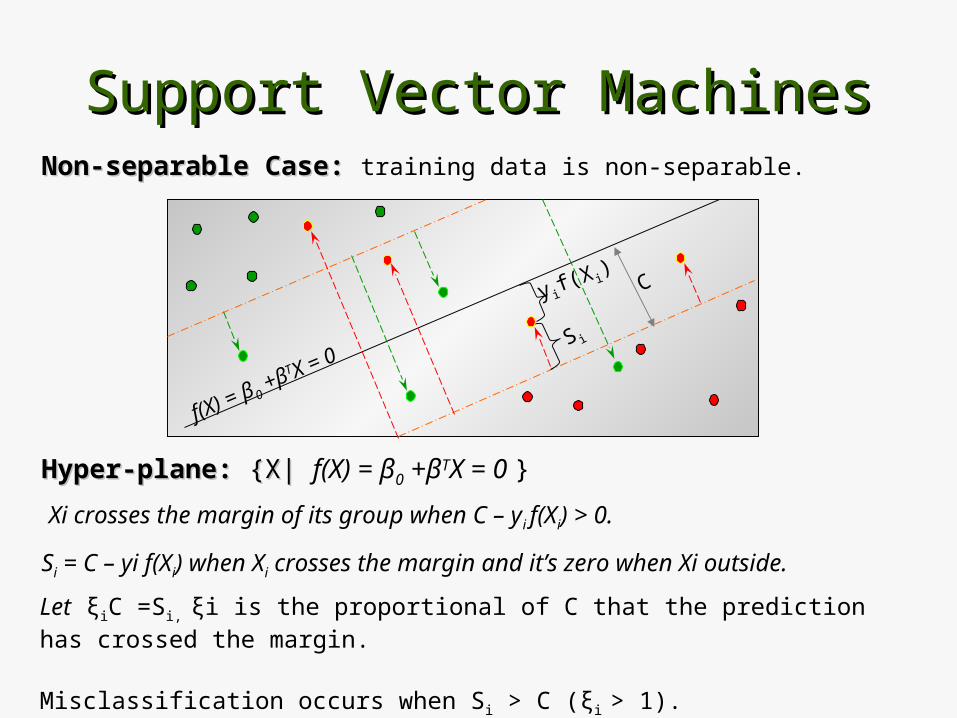
Hyper-plane:Hyper-plane: {X| {X| f(X) = β0 +βTX = 0 }
Non-separable Case:Non-separable Case: training data is non-separable.
f(X) = β 0 +βT X = 0
Si = C – yi f(Xi) when Xi crosses the margin and it’s zero when Xi outside.
Xi crosses the margin of its group when C – yi f(Xi) > 0.
y if(X i)
S i
C
Let ξiC =Si, ξi is the proportional of C that the prediction has crossed the margin.
Misclassification occurs when Si > C (ξi > 1).
Support Vector MachinesSupport Vector Machines
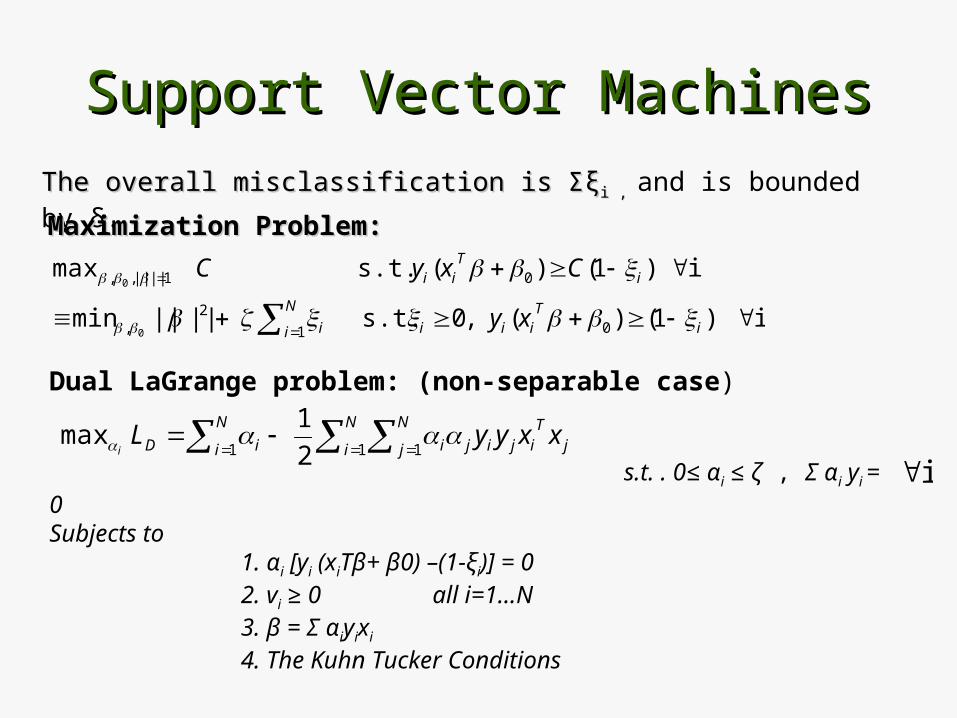
The overall misclassification is The overall misclassification is ΣξΣξi , i , and is bounded by δ.
i )1()( ,0 s.t. ||||min
i )1()( s.t. max
01
2,
01||||,,
0
0
iT
iii
N
i i
iT
ii
xy
CxyC
Maximization Problem:Maximization Problem:
N
i
N
j jT
ijiji
N
i iD xxyyLi 1 11 2
1 max
Dual LaGrange problem: (non-separable case)
s.t. . 0≤ αi ≤ ζ , Σ αi yi = 0Subjects to
1. αi [yi (xiTβ+ β0) –(1-ξi)] = 02. vi ≥ 0 all i=1…N3. β = Σ αiyixi
4. The Kuhn Tucker Conditions
i
Support Vector MachinesSupport Vector Machines
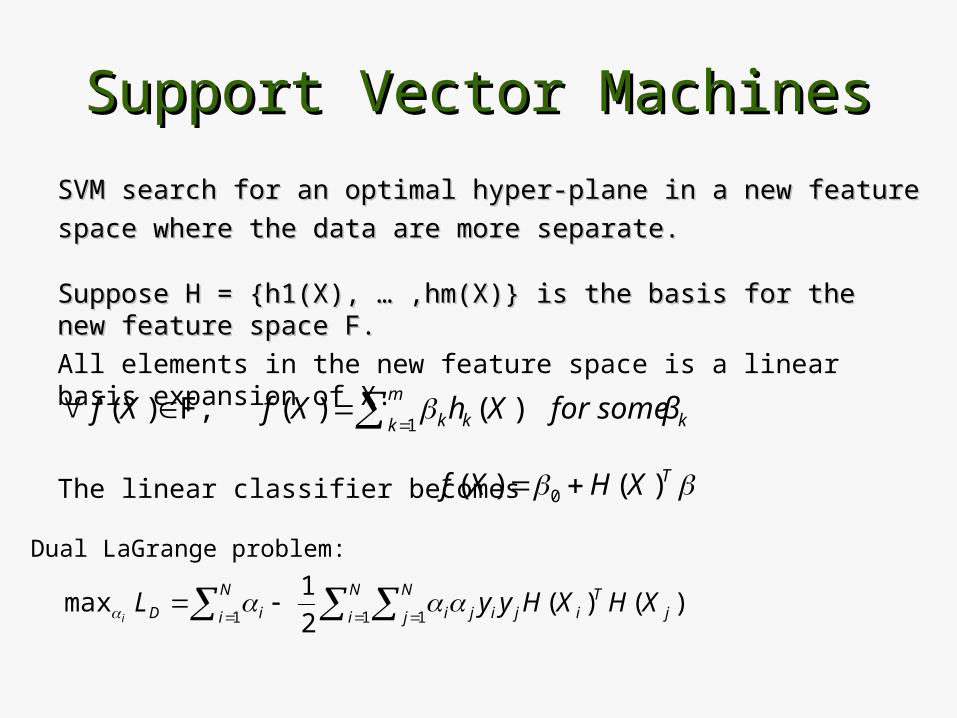
SVM search for an optimal hyper-plane in a new feature SVM search for an optimal hyper-plane in a new feature
space where the data are more separate.space where the data are more separate.
)()( )( 1 k
m
k kk β for some XhXfXf F,
The linear classifier becomes TXHXf )()( 0
N
i
N
j jT
ijiji
N
i iD XHXHyyLi 1 11
)()(2
1 max
Dual LaGrange problem:
Suppose H = {h1(X), … ,hm(X)} is the basis for the new feature space F.Suppose H = {h1(X), … ,hm(X)} is the basis for the new feature space F.
All elements in the new feature space is a linear basis expansion of X.
Support Vector MachinesSupport Vector Machines
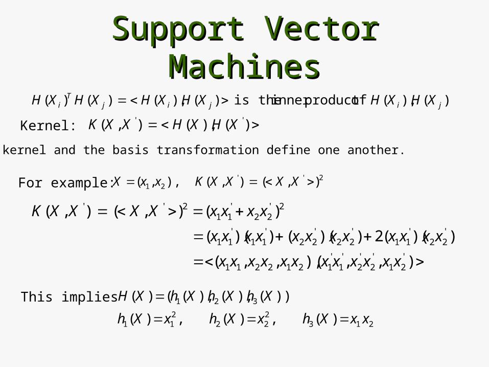
).(),( ofproduct inner theis )(),( )()( jijijT
i XHXHXHXHXHXH
For example: 2''21 ),( ),( ),,( XXXXKxxX
),,(),,,(
))((2))(())((
)(),( ),(
'21
'2
'2
'1
'1212211
'22
'11
'22
'22
'11
'11
2'22
'11
2''
xxxxxxxxxxxx
xxxxxxxxxxxx
xxxxXXXXK
)(),( ),( '' XHXHXXKKernel:
This implies
213222
211
321
)(,)(,)(
))(),(),(()(
xxXhxXhxXh
XhXhXhXH
The kernel and the basis transformation define one another.

Support Vector MachinesSupport Vector Machines
N
i
N
j jijiji
N
i iD XXKyyL1 11
),(2
1
Dual LaGrange function:
This shows the basis transformation in SVM does not need to be define explicitly.
)/||||(exp ),( '' XXXXK
The most common kernels:
1. dth Degree Polynomial:
2. Radial Basis:
3. Neural Network:
d'' ),1( ),( XXXXK
),( tanh ),( 2'
1' CXXCXXK
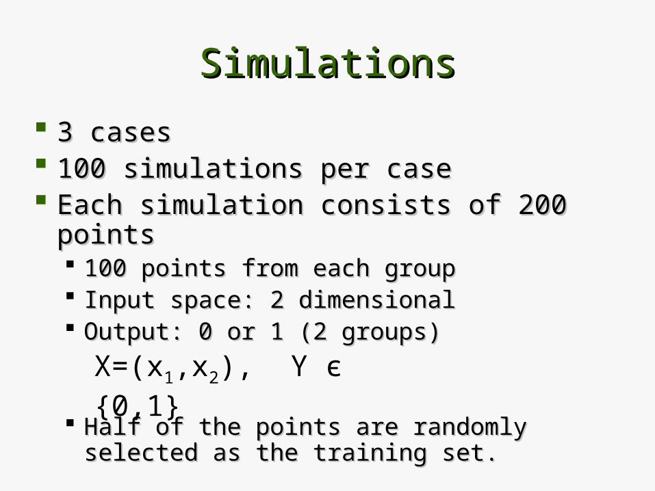
SimulationsSimulations
3 cases3 cases 100 simulations per case100 simulations per case Each simulation consists of 200 points Each simulation consists of 200 points
100 points from each group100 points from each group Input space: 2 dimensionalInput space: 2 dimensional Output: 0 or 1 (2 groups)Output: 0 or 1 (2 groups)
Half of the points are randomly selected as Half of the points are randomly selected as the training set.the training set.
X=(x1,x2), Y є {0,1}
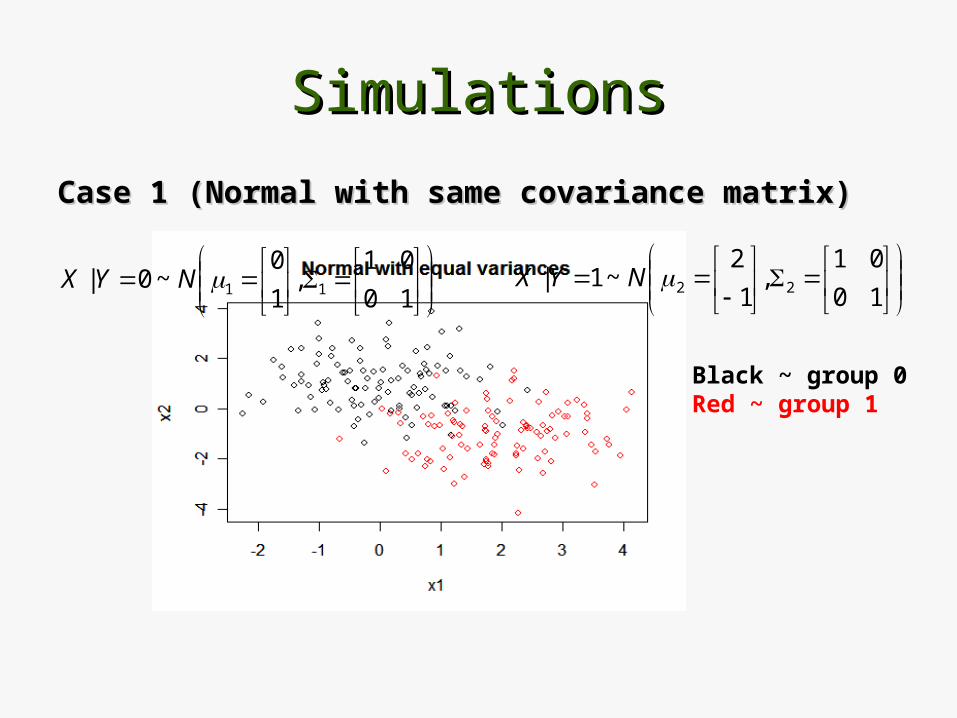
SimulationsSimulations
Case 1 (Normal with same covariance matrix)Case 1 (Normal with same covariance matrix)
Black ~ group 0Red ~ group 1
10
01,
1
0~0| 11NYX
10
01,
1
2~1| 22NYX
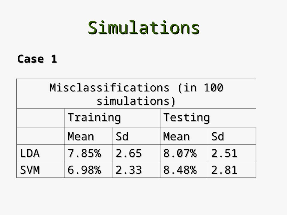
SimulationsSimulations
Case 1Case 1
Misclassifications (in 100 simulations)Misclassifications (in 100 simulations)
TrainingTraining TestingTesting
MeanMean SdSd MeanMean SdSd
LDALDA 7.85%7.85% 2.652.65 8.07%8.07% 2.512.51
SVMSVM 6.98%6.98% 2.332.33 8.48%8.48% 2.812.81
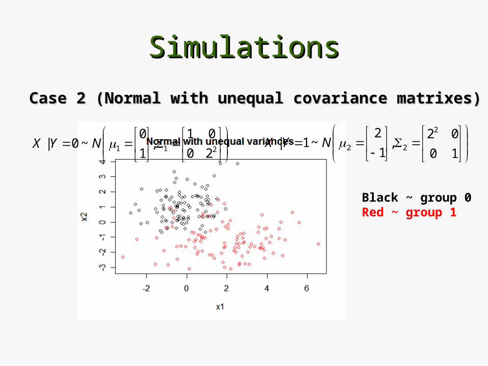
SimulationsSimulations
Case 2 (Normal with unequal covariance matrixes)Case 2 (Normal with unequal covariance matrixes)
Black ~ group 0Red ~ group 1
211 20
01,
1
0~0| NYX
10
02,
1
2~1|
2
22NYX

SimulationsSimulations
Case 2Case 2
Misclassifications (in 100 simulations)Misclassifications (in 100 simulations)
TrainingTraining TestingTesting
MeanMean SdSd MeanMean SdSd
QDAQDA 15.5%15.5% 3.753.75 16.84%16.84% 3.483.48
SVMSVM 13.6%13.6% 4.034.03 18.8%18.8% 4.014.01
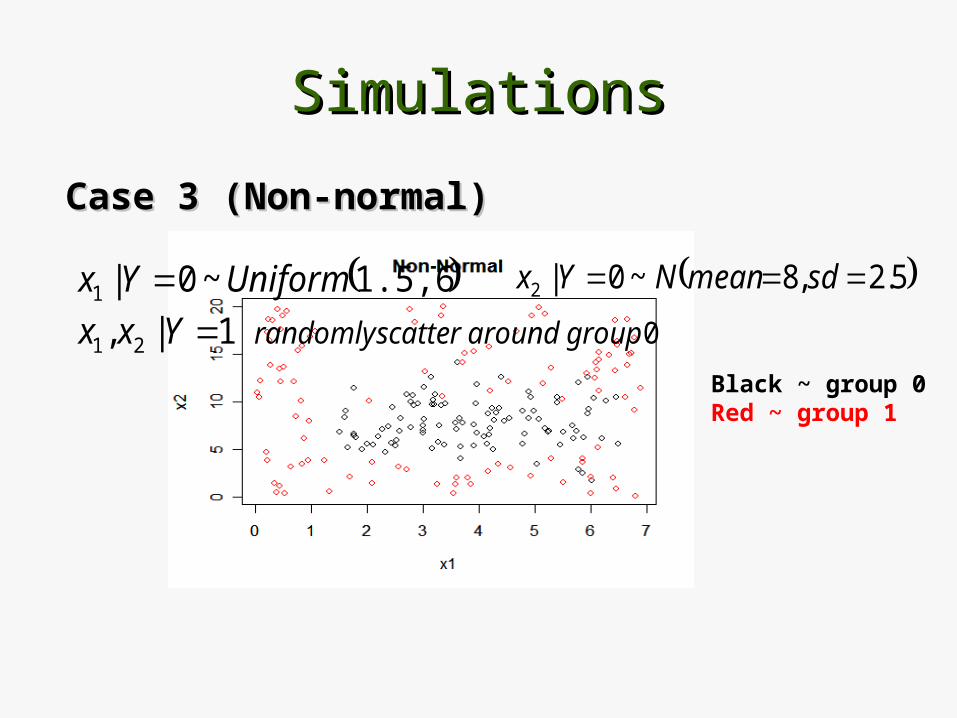
SimulationsSimulations
Case 3 (Non-normal)Case 3 (Non-normal)
Black ~ group 0Red ~ group 1
1.5,6.5 ~0|1 UniformYx 5.2,8~0|2 sdmeanNYx
0 1|, 21 group aroundscatter randomlyYxx
SimulationsSimulations
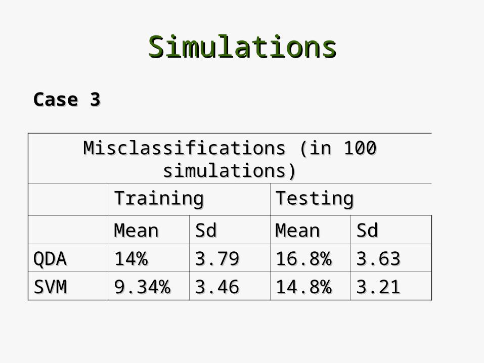
Case 3Case 3
Misclassifications (in 100 simulations)Misclassifications (in 100 simulations)
TrainingTraining TestingTesting
MeanMean SdSd MeanMean SdSd
QDAQDA 14%14% 3.793.79 16.8%16.8% 3.633.63
SVMSVM 9.34%9.34% 3.463.46 14.8%14.8% 3.213.21
SimulationsSimulations
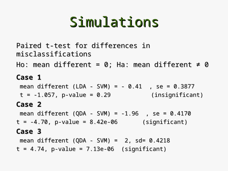
Paired t-test for differences in misclassifications Paired t-test for differences in misclassifications
Ho: Ho: mean different = 0; mean different = 0; Ha: Ha: mean different mean different ≠≠ 0 0
Case 1 Case 1 mean different (LDA - SVM) = - 0.41 , se = 0.3877mean different (LDA - SVM) = - 0.41 , se = 0.3877
t = -1.057, p-value = 0.29 t = -1.057, p-value = 0.29 (insignificant)(insignificant)
Case 2Case 2 mean different (QDA - SVM) = -1.96 , se = 0.4170mean different (QDA - SVM) = -1.96 , se = 0.4170
t = -4.70, p-value = 8.42e-06 t = -4.70, p-value = 8.42e-06 (significant)(significant)
Case 3Case 3 mean different (QDA - SVM) = 2, sd= 0.4218mean different (QDA - SVM) = 2, sd= 0.4218
t = 4.74, p-value = 7.13e-06 t = 4.74, p-value = 7.13e-06 (significant)(significant)
RemarksRemarks
Support Vector MachinesSupport Vector Machines Maps the original input space onto a feature space of higher dimension Maps the original input space onto a feature space of higher dimension No assumption on the distributions of X’sNo assumption on the distributions of X’s
PerformancePerformance The performances of Discriminant Analysis and SVM are similar (when (X|The performances of Discriminant Analysis and SVM are similar (when (X|
Y) has a Normal distribution and share the same Y) has a Normal distribution and share the same ΣΣ))
Discriminant Analysis has a better performanceDiscriminant Analysis has a better performance
(when the covariance matrices for the two groups are different)(when the covariance matrices for the two groups are different)
SVM has a better performanceSVM has a better performance
(when the input (X) violated the distribution assumption)(when the input (X) violated the distribution assumption)
ReferenceReference1. N. Cristianini, and J. Shawe-Taylor An introduction to Support Vector
Machines and other kernel-based learning methods. New York: Cambridge University Press, 2000.
2. J. Friedman, T. Hastie, and R. Tibshirani The Elements of Statistical Learning. NewYork: Springer, 2001.
3. D. Meyer, C. Chang, and C. Lin. R Documentation: Support Vector Machines. http://www.maths.lth.se/help/R/.R/library/e1071/html/svm.html Last updated: March 2006
4. H. Planatscher and J. Dietzsch. SVM-Tutorial using R (e1071-package) http://www.potschi.de/svmtut/svmtut.htm
5. M. Van Den Heuvel, J. Horrocks, S. Bashar, S. Taylor, S. Burke, K. Hatta, E. Lewis, and A. Croy. Menstrual Cycle Hormones Induce Changes in Functional Interac-tions Between Lymphocytes and Endothelial Cells. Journal of Clinical Endocrinology and Metabolism, 2005.