•••

Support Vector Machines for Binary Classification

Understanding Support Vector MachinesSeparable DataNonseparable DataNonlinear Transformation with Kernels

Separable DataYou can use a support vector machine (SVM) when your data has exactly two classes. An SVM classifies data byfinding the best hyperplane that separates all data points of one class from those of the other class. The besthyperplane for an SVM means the one with the largest margin between the two classes. Margin means the maximalwidth of the slab parallel to the hyperplane that has no interior data points.

The support vectors are the data points that are closest to the separating hyperplane; these points are on theboundary of the slab. The following figure illustrates these definitions, with + indicating data points of type 1, and –indicating data points of type –1.

Mathematical Formulation: Primal. This discussion follows Hastie, Tibshirani, and Friedman [1] and Christianiniand Shawe-Taylor [2].

The data for training is a set of points (vectors) x along with their categories y . For some dimension d, the x  ∊ R ,and the y  = ±1. The equation of a hyperplane is

where β ∊ R and b is a real number.

The following problem defines the best separating hyperplane (i.e., the decision boundary). Find β and b thatminimize ||β|| such that for all data points (x ,y ),

The support vectors are the x on the boundary, those for which

For mathematical convenience, the problem is usually given as the equivalent problem of minimizing . This is aquadratic programming problem. The optimal solution enables classification of a vector z as follows:

is the classification score and represents the distance z is from the decision boundary.

Mathematical Formulation: Dual. It is computationally simpler to solve the dual quadratic programming problem.To obtain the dual, take positive Lagrange multipliers α multiplied by each constraint, and subtract from the objectivefunction:

where you look for a stationary point of L over β and b. Setting the gradient of L to 0, you get

(1)

j j jd

j

f (x) = x′β + b = 0

d

j j

y j f (x j) ≥ 1.

j y j f (x j) = 1.

β(ˆβ, ˆb

)

class(z) = sign(z′ˆβ + ˆb

)= sign

(ˆf (z)

).

ˆf (z)

j

LP = 1

2β′β −

j

α j(y j(x j′β + b) − 1),

P P

β

0

=

j

α jy jx j

=

j

α jy j.

•

•

Substituting into L , you get the dual L :

which you maximize over α  ≥ 0. In general, many α are 0 at the maximum. The nonzero α in the solution to the dualproblem define the hyperplane, as seen in Equation 1, which gives β as the sum of α y x . The data points xcorresponding to nonzero α are the support vectors.

The derivative of L with respect to a nonzero α is 0 at an optimum. This gives

In particular, this gives the value of b at the solution, by taking any j with nonzero α .

The dual is a standard quadratic programming problem. For example, the Optimization Toolbox™ quadprog solversolves this type of problem.

Nonseparable DataYour data might not allow for a separating hyperplane. In that case, SVM can use a soft margin, meaning ahyperplane that separates many, but not all data points.

There are two standard formulations of soft margins. Both involve adding slack variables ξ and a penalty parameterC.

The L -norm problem is:

such that

The L -norm refers to using ξ as slack variables instead of their squares. The three solver options SMO, ISDA,and L1QP of fitcsvm minimize the L -norm problem.

The L -norm problem is:

subject to the same constraints.

In these formulations, you can see that increasing C places more weight on the slack variables ξ , meaning theoptimization attempts to make a stricter separation between classes. Equivalently, reducing C towards 0 makesmisclassification less important.

Mathematical Formulation: Dual. For easier calculations, consider the L dual problem to this soft-marginformulation. Using Lagrange multipliers μ , the function to minimize for the L -norm problem is:

where you look for a stationary point of L over β, b, and positive ξ . Setting the gradient of L to 0, you get

These equations lead directly to the dual formulation:

subject to the constraints

P D

LD =

j

α j −1

2

j

k

α jαky jykx j′xk,

j j j

j j j j

j

D j

y j f (x j) − 1 = 0.

j

j

1

minβ,b,ξ

(1

2β′β + C

j

ξ j

)

y j f (x j)

ξ j

≥ 1 − ξ j

≥ 0.

1j

1

2

minβ,b,ξ

(1

2β′β + C

j

ξ2j

)

j

1

j1

LP = 1

2β′β + C

j

ξ j −

j

α j(yi f (x j) − (1 − ξ j)) −

j

μ jξ j,

P j P

β

j

α jy j

α j

α j, μ j, ξ j

=

j

α jy jx j

= 0

= C − μ j

≥ 0.

maxα

j

α j −1

2

j

k

α jαky jykx j′xk

j

y jα j = 0

0 ≤ α j ≤ C .

•

•

•

•

˗

˗

˗

˗

˗

•

•

The final set of inequalities, 0 ≤ α  ≤ C, shows why C is sometimes called a box constraint. C keeps the allowablevalues of the Lagrange multipliers α in a “box”, a bounded region.

The gradient equation for b gives the solution b in terms of the set of nonzero α , which correspond to the supportvectors.

You can write and solve the dual of the L -norm problem in an analogous manner. For details, see Christianini andShawe-Taylor [2], Chapter 6.

fitcsvm Implementation. Both dual soft-margin problems are quadratic programming problems. Internally,fitcsvm has several different algorithms for solving the problems.

For one-class or binary classification, if you do not set a fraction of expected outliers in the data (seeOutlierFraction), then the default solver is Sequential Minimal Optimization (SMO). SMO minimizes the one-norm problem by a series of two-point minimizations. During optimization, SMO respects the linear constraint

and explicitly includes the bias term in the model. SMO is relatively fast. For more details on SMO,

see [3].For binary classification, if you set a fraction of expected outliers in the data, then the default solver is theIterative Single Data Algorithm. Like SMO, ISDA solves the one-norm problem. Unlike SMO, ISDA minimizes bya series on one-point minimizations, does not respect the linear constraint, and does not explicitly include thebias term in the model. For more details on ISDA, see [4].For one-class or binary classification, and if you have an Optimization Toolbox license, you can choose to usequadprog to solve the one-norm problem. quadprog uses a good deal of memory, but solves quadratic programsto a high degree of precision. For more details, see Quadratic Programming Definition (Optimization Toolbox).

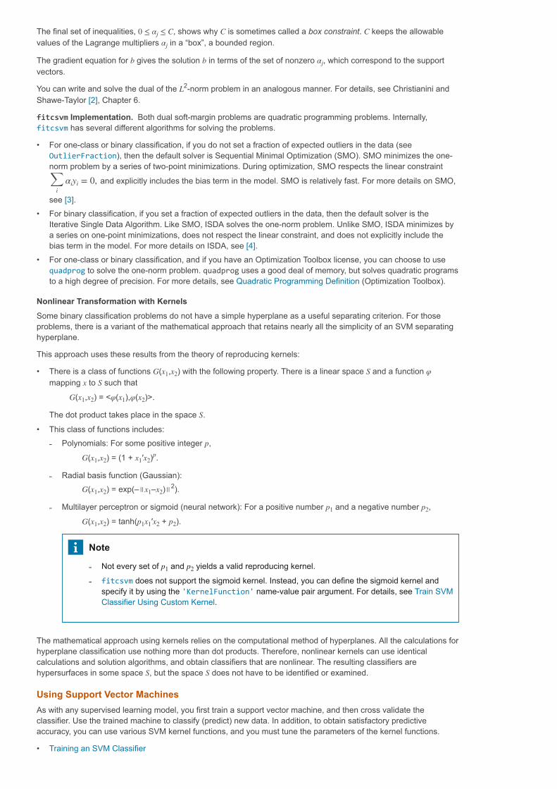
Nonlinear Transformation with KernelsSome binary classification problems do not have a simple hyperplane as a useful separating criterion. For thoseproblems, there is a variant of the mathematical approach that retains nearly all the simplicity of an SVM separatinghyperplane.

This approach uses these results from the theory of reproducing kernels:

There is a class of functions G(x ,x ) with the following property. There is a linear space S and a function φmapping x to S such that

G(x ,x ) = <φ(x ),φ(x )>.

The dot product takes place in the space S.

This class of functions includes:Polynomials: For some positive integer p,

G(x ,x ) = (1 + x ′x ) .

Radial basis function (Gaussian):G(x ,x ) = exp(–∥x –x )∥ ).

Multilayer perceptron or sigmoid (neural network): For a positive number p and a negative number p ,

G(x ,x ) = tanh(p x ′x + p ).

Note

Not every set of p and p yields a valid reproducing kernel.

fitcsvm does not support the sigmoid kernel. Instead, you can define the sigmoid kernel andspecify it by using the 'KernelFunction' name-value pair argument. For details, see Train SVMClassifier Using Custom Kernel.

The mathematical approach using kernels relies on the computational method of hyperplanes. All the calculations forhyperplane classification use nothing more than dot products. Therefore, nonlinear kernels can use identicalcalculations and solution algorithms, and obtain classifiers that are nonlinear. The resulting classifiers arehypersurfaces in some space S, but the space S does not have to be identified or examined.

Using Support Vector MachinesAs with any supervised learning model, you first train a support vector machine, and then cross validate theclassifier. Use the trained machine to classify (predict) new data. In addition, to obtain satisfactory predictiveaccuracy, you can use various SVM kernel functions, and you must tune the parameters of the kernel functions.

Training an SVM Classifier

j

j

j

2

i

αiyi = 0,

1 2

1 2 1 2

1 2 1 2p

1 2 1 22

1 2

1 2 1 1 2 2

1 2

••

••

•

•

•

Classifying New Data with an SVM ClassifierTuning an SVM Classifier

Training an SVM ClassifierTrain, and optionally cross validate, an SVM classifier using fitcsvm. The most common syntax is:

SVMModel = fitcsvm(X,Y,'KernelFunction','rbf',... 'Standardize',true,'ClassNames',{'negClass','posClass'});

The inputs are:

X — Matrix of predictor data, where each row is one observation, and each column is one predictor.Y — Array of class labels with each row corresponding to the value of the corresponding row in X. Y can be acategorical, character, or string array, a logical or numeric vector, or a cell array of character vectors.KernelFunction — The default value is 'linear' for two-class learning, which separates the data by ahyperplane. The value 'gaussian' (or 'rbf') is the default for one-class learning, and specifies to use theGaussian (or radial basis function) kernel. An important step to successfully train an SVM classifier is to choosean appropriate kernel function.Standardize — Flag indicating whether the software should standardize the predictors before training theclassifier.ClassNames — Distinguishes between the negative and positive classes, or specifies which classes to include inthe data. The negative class is the first element (or row of a character array), e.g., 'negClass', and the positiveclass is the second element (or row of a character array), e.g., 'posClass'. ClassNames must be the same datatype as Y. It is good practice to specify the class names, especially if you are comparing the performance ofdifferent classifiers.

The resulting, trained model (SVMModel) contains the optimized parameters from the SVM algorithm, enabling you toclassify new data.

For more name-value pairs you can use to control the training, see the fitcsvm reference page.

Classifying New Data with an SVM ClassifierClassify new data using predict. The syntax for classifying new data using a trained SVM classifier (SVMModel) is:

[label,score] = predict(SVMModel,newX);

The resulting vector, label, represents the classification of each row in X. score is an n-by-2 matrix of soft scores.Each row corresponds to a row in X, which is a new observation. The first column contains the scores for theobservations being classified in the negative class, and the second column contains the scores observations beingclassified in the positive class.

To estimate posterior probabilities rather than scores, first pass the trained SVM classifier (SVMModel) tofitPosterior, which fits a score-to-posterior-probability transformation function to the scores. The syntax is:

ScoreSVMModel = fitPosterior(SVMModel,X,Y);

The property ScoreTransform of the classifier ScoreSVMModel contains the optimal transformation function. PassScoreSVMModel to predict. Rather than returning the scores, the output argument score contains the posteriorprobabilities of an observation being classified in the negative (column 1 of score) or positive (column 2 of score)class.

Tuning an SVM ClassifierUse the 'OptimizeHyperparameters' name-value pair argument of fitcsvm to find parameter values thatminimize the cross-validation loss. The eligible parameters are 'BoxConstraint', 'KernelFunction','KernelScale', 'PolynomialOrder', and 'Standardize'. For an example, see Optimize an SVM Classifier FitUsing Bayesian Optimization. Alternatively, you can use the bayesopt function, as shown in Optimize a Cross-Validated SVM Classifier Using bayesopt. The bayesopt function allows more flexibility to customize optimization.You can use the bayesopt function to optimize any parameters, including parameters that are not eligible to optimizewhen you use the fitcsvm function.

You can also try tuning parameters of your classifier manually according to this scheme:

1. Pass the data to fitcsvm, and set the name-value pair argument 'KernelScale','auto'. Suppose that thetrained SVM model is called SVMModel. The software uses a heuristic procedure to select the kernel scale. Theheuristic procedure uses subsampling. Therefore, to reproduce results, set a random number seed using rngbefore training the classifier.

2. Cross validate the classifier by passing it to crossval. By default, the software conducts 10-fold crossvalidation.

3. Pass the cross-validated SVM model to kfoldLoss to estimate and retain the classification error.

•

•

4. Retrain the SVM classifier, but adjust the 'KernelScale' and 'BoxConstraint' name-value pair arguments.BoxConstraint — One strategy is to try a geometric sequence of the box constraint parameter. Forexample, take 11 values, from 1e-5 to 1e5 by a factor of 10. Increasing BoxConstraint might decrease thenumber of support vectors, but also might increase training time.KernelScale — One strategy is to try a geometric sequence of the RBF sigma parameter scaled at theoriginal kernel scale. Do this by:

a. Retrieving the original kernel scale, e.g., ks, using dot notation: ks =SVMModel.KernelParameters.Scale.

b. Use as new kernel scales factors of the original. For example, multiply ks by the 11 values 1e-5 to 1e5,increasing by a factor of 10.

Choose the model that yields the lowest classification error. You might want to further refine your parameters toobtain better accuracy. Start with your initial parameters and perform another cross-validation step, this time using afactor of 1.2.

Train SVM Classifiers Using a Gaussian KernelThis example shows how to generate a nonlinear classifier withGaussian kernel function. First, generate one class of points inside theunit disk in two dimensions, and another class of points in the annulusfrom radius 1 to radius 2. Then, generates a classifier based on the data with the Gaussian radial basis functionkernel. The default linear classifier is obviously unsuitable for this problem, since the model is circularly symmetric.Set the box constraint parameter to Inf to make a strict classification, meaning no misclassified training points.Other kernel functions might not work with this strict box constraint, since they might be unable to provide a strictclassification. Even though the rbf classifier can separate the classes, the result can be overtrained.

Generate 100 points uniformly distributed in the unit disk. To do so, generate a radius r as the square root of auniform random variable, generate an angle t uniformly in (0, ), and put the point at (r cos(t), r sin(t)).

rng(1); % For reproducibility r = sqrt(rand(100,1)); % Radius t = 2*pi*rand(100,1); % Angle data1 = [r.*cos(t), r.*sin(t)]; % Points

Generate 100 points uniformly distributed in the annulus. The radius is again proportional to a square root, this timea square root of the uniform distribution from 1 through 4.

r2 = sqrt(3*rand(100,1)+1); % Radius t2 = 2*pi*rand(100,1); % Angle data2 = [r2.*cos(t2), r2.*sin(t2)]; % points

Plot the points, and plot circles of radii 1 and 2 for comparison.

figure; plot(data1(:,1),data1(:,2),'r.','MarkerSize',15) hold on plot(data2(:,1),data2(:,2),'b.','MarkerSize',15) ezpolar(@(x)1);ezpolar(@(x)2); axis equal hold off

Try it in MATLAB

2π

Put the data in one matrix, and make a vector of classifications.

data3 = [data1;data2]; theclass = ones(200,1); theclass(1:100) = -1;

Train an SVM classifier with KernelFunction set to 'rbf' and BoxConstraint set to Inf. Plot the decisionboundary and flag the support vectors.

%Train the SVM Classifier cl = fitcsvm(data3,theclass,'KernelFunction','rbf',... 'BoxConstraint',Inf,'ClassNames',[-1,1]); % Predict scores over the grid d = 0.02; [x1Grid,x2Grid] = meshgrid(min(data3(:,1)):d:max(data3(:,1)),... min(data3(:,2)):d:max(data3(:,2))); xGrid = [x1Grid(:),x2Grid(:)]; [~,scores] = predict(cl,xGrid); % Plot the data and the decision boundary figure; h(1:2) = gscatter(data3(:,1),data3(:,2),theclass,'rb','.'); hold on ezpolar(@(x)1); h(3) = plot(data3(cl.IsSupportVector,1),data3(cl.IsSupportVector,2),'ko'); contour(x1Grid,x2Grid,reshape(scores(:,2),size(x1Grid)),[0 0],'k'); legend(h,{'-1','+1','Support Vectors'}); axis equal hold off

fitcsvm generates a classifier that is close to a circle of radius 1. The difference is due to the random training data.

Training with the default parameters makes a more nearly circular classification boundary, but one that misclassifiessome training data. Also, the default value of BoxConstraint is 1, and, therefore, there are more support vectors.

cl2 = fitcsvm(data3,theclass,'KernelFunction','rbf'); [~,scores2] = predict(cl2,xGrid); figure; h(1:2) = gscatter(data3(:,1),data3(:,2),theclass,'rb','.'); hold on ezpolar(@(x)1); h(3) = plot(data3(cl2.IsSupportVector,1),data3(cl2.IsSupportVector,2),'ko'); contour(x1Grid,x2Grid,reshape(scores2(:,2),size(x1Grid)),[0 0],'k'); legend(h,{'-1','+1','Support Vectors'}); axis equal hold off

Train SVM Classifier Using Custom KernelThis example shows how to use a custom kernel function, such as thesigmoid kernel, to train SVM classifiers, and adjust custom kernelfunction parameters.

Generate a random set of points within the unit circle. Label points in the first and third quadrants as belonging to thepositive class, and those in the second and fourth quadrants in the negative class.

rng(1); % For reproducibility n = 100; % Number of points per quadrant r1 = sqrt(rand(2*n,1)); % Random radii t1 = [pi/2*rand(n,1); (pi/2*rand(n,1)+pi)]; % Random angles for Q1 and Q3 X1 = [r1.*cos(t1) r1.*sin(t1)]; % Polar-to-Cartesian conversion r2 = sqrt(rand(2*n,1)); t2 = [pi/2*rand(n,1)+pi/2; (pi/2*rand(n,1)-pi/2)]; % Random angles for Q2 and Q4 X2 = [r2.*cos(t2) r2.*sin(t2)]; X = [X1; X2]; % Predictors Y = ones(4*n,1); Y(2*n + 1:end) = -1; % Labels

Plot the data.

figure; gscatter(X(:,1),X(:,2),Y); title('Scatter Diagram of Simulated Data')

Write a function that accepts two matrices in the feature space as inputs, and transforms them into a Gram matrixusing the sigmoid kernel.

function G = mysigmoid(U,V) % Sigmoid kernel function with slope gamma and intercept c gamma = 1; c = -1; G = tanh(gamma*U*V' + c); end

Save this code as a file named mysigmoid on your MATLAB® path.

Train an SVM classifier using the sigmoid kernel function. It is good practice to standardize the data.

Try it in MATLAB

Mdl1 = fitcsvm(X,Y,'KernelFunction','mysigmoid','Standardize',true);

Mdl1 is a ClassificationSVM classifier containing the estimated parameters.

Plot the data, and identify the support vectors and the decision boundary.

% Compute the scores over a grid d = 0.02; % Step size of the grid [x1Grid,x2Grid] = meshgrid(min(X(:,1)):d:max(X(:,1)),... min(X(:,2)):d:max(X(:,2))); xGrid = [x1Grid(:),x2Grid(:)]; % The grid [~,scores1] = predict(Mdl1,xGrid); % The scores figure; h(1:2) = gscatter(X(:,1),X(:,2),Y); hold on h(3) = plot(X(Mdl1.IsSupportVector,1),... X(Mdl1.IsSupportVector,2),'ko','MarkerSize',10); % Support vectors contour(x1Grid,x2Grid,reshape(scores1(:,2),size(x1Grid)),[0 0],'k'); % Decision boundary title('Scatter Diagram with the Decision Boundary') legend({'-1','1','Support Vectors'},'Location','Best'); hold off

You can adjust the kernel parameters in an attempt to improve the shape of the decision boundary. This might alsodecrease the within-sample misclassification rate, but, you should first determine the out-of-sample misclassificationrate.

Determine the out-of-sample misclassification rate by using 10-fold cross validation.

CVMdl1 = crossval(Mdl1); misclass1 = kfoldLoss(CVMdl1); misclass1

misclass1 = 0.1375

The out-of-sample misclassification rate is 13.5%.

Write another sigmoid function, but Set gamma = 0.5;.

function G = mysigmoid2(U,V) % Sigmoid kernel function with slope gamma and intercept c gamma = 0.5; c = -1; G = tanh(gamma*U*V' + c); end

Save this code as a file named mysigmoid2 on your MATLAB® path.

Train another SVM classifier using the adjusted sigmoid kernel. Plot the data and the decision region, and determinethe out-of-sample misclassification rate.

Mdl2 = fitcsvm(X,Y,'KernelFunction','mysigmoid2','Standardize',true); [~,scores2] = predict(Mdl2,xGrid); figure; h(1:2) = gscatter(X(:,1),X(:,2),Y); hold on h(3) = plot(X(Mdl2.IsSupportVector,1),... X(Mdl2.IsSupportVector,2),'ko','MarkerSize',10); title('Scatter Diagram with the Decision Boundary') contour(x1Grid,x2Grid,reshape(scores2(:,2),size(x1Grid)),[0 0],'k'); legend({'-1','1','Support Vectors'},'Location','Best'); hold off CVMdl2 = crossval(Mdl2); misclass2 = kfoldLoss(CVMdl2); misclass2

misclass2 = 0.0450

After the sigmoid slope adjustment, the new decision boundary seems to provide a better within-sample fit, and thecross-validation rate contracts by more than 66%.

Optimize an SVM Classifier Fit Using Bayesian OptimizationThis example shows how to optimize an SVM classification using thefitcsvm function and OptimizeHyperparameters name-value pair.The classification works on locations of points from a Gaussian mixturemodel. In The Elements of Statistical Learning, Hastie, Tibshirani, and Friedman (2009), page 17 describes the

Try it in MATLAB

model. The model begins with generating 10 base points for a "green" class, distributed as 2-D independent normalswith mean (1,0) and unit variance. It also generates 10 base points for a "red" class, distributed as 2-D independentnormals with mean (0,1) and unit variance. For each class (green and red), generate 100 random points as follows:

1. Choose a base point m of the appropriate color uniformly at random.

2. Generate an independent random point with 2-D normal distribution with mean m and variance I/5, where I is the2-by-2 identity matrix. In this example, use a variance I/50 to show the advantage of optimization more clearly.

Generate the Points and Classifier

Generate the 10 base points for each class.

rng default % For reproducibility grnpop = mvnrnd([1,0],eye(2),10); redpop = mvnrnd([0,1],eye(2),10);

View the base points.

plot(grnpop(:,1),grnpop(:,2),'go') hold on plot(redpop(:,1),redpop(:,2),'ro') hold off

Since some red base points are close to green base points, it can be difficult to classify the data points based onlocation alone.

Generate the 100 data points of each class.

redpts = zeros(100,2);grnpts = redpts; for i = 1:100 grnpts(i,:) = mvnrnd(grnpop(randi(10),:),eye(2)*0.02); redpts(i,:) = mvnrnd(redpop(randi(10),:),eye(2)*0.02); end

View the data points.

figure plot(grnpts(:,1),grnpts(:,2),'go') hold on plot(redpts(:,1),redpts(:,2),'ro') hold off

Prepare Data For Classification

Put the data into one matrix, and make a vector grp that labels the class of each point.

cdata = [grnpts;redpts]; grp = ones(200,1); % Green label 1, red label -1 grp(101:200) = -1;

Prepare Cross-Validation

Set up a partition for cross-validation. This step fixes the train and test sets that the optimization uses at each step.

c = cvpartition(200,'KFold',10);

Optimize the Fit

To find a good fit, meaning one with a low cross-validation loss, set options to use Bayesian optimization. Use thesame cross-validation partition c in all optimizations.

For reproducibility, use the 'expected-improvement-plus' acquisition function.

opts = struct('Optimizer','bayesopt','ShowPlots',true,'CVPartition',c,... 'AcquisitionFunctionName','expected-improvement-plus'); svmmod = fitcsvm(cdata,grp,'KernelFunction','rbf',... 'OptimizeHyperparameters','auto','HyperparameterOptimizationOptions',opts)

|=====================================================================================================| | Iter | Eval | Objective | Objective | BestSoFar | BestSoFar | BoxConstraint| KernelScale | | | result | | runtime | (observed) | (estim.) | | | |=====================================================================================================| | 1 | Best | 0.345 | 0.34358 | 0.345 | 0.345 | 0.00474 | 306.44 | | 2 | Best | 0.115 | 0.3085 | 0.115 | 0.12678 | 430.31 | 1.4864 | | 3 | Accept | 0.52 | 0.36849 | 0.115 | 0.1152 | 0.028415 | 0.014369 | | 4 | Accept | 0.61 | 0.16208 | 0.115 | 0.11504 | 133.94 | 0.0031427 | | 5 | Accept | 0.34 | 0.25453 | 0.115 | 0.11504 | 0.010993 | 5.7742 | | 6 | Best | 0.085 | 0.15841 | 0.085 | 0.085039 | 885.63 | 0.68403 | | 7 | Accept | 0.105 | 0.29711 | 0.085 | 0.085428 | 0.3057 | 0.58118 |

| 8 | Accept | 0.21 | 0.52313 | 0.085 | 0.09566 | 0.16044 | 0.91824 | | 9 | Accept | 0.085 | 0.21356 | 0.085 | 0.08725 | 972.19 | 0.46259 | | 10 | Accept | 0.1 | 0.18961 | 0.085 | 0.090952 | 990.29 | 0.491 | | 11 | Best | 0.08 | 0.16313 | 0.08 | 0.079362 | 2.5195 | 0.291 | | 12 | Accept | 0.09 | 0.15401 | 0.08 | 0.08402 | 14.338 | 0.44386 | | 13 | Accept | 0.1 | 0.34121 | 0.08 | 0.08508 | 0.0022577 | 0.23803 | | 14 | Accept | 0.11 | 0.36934 | 0.08 | 0.087378 | 0.2115 | 0.32109 | | 15 | Best | 0.07 | 0.39858 | 0.07 | 0.081507 | 910.2 | 0.25218 | | 16 | Best | 0.065 | 0.18705 | 0.065 | 0.072457 | 953.22 | 0.26253 | | 17 | Accept | 0.075 | 0.30259 | 0.065 | 0.072554 | 998.74 | 0.23087 | | 18 | Accept | 0.295 | 0.22177 | 0.065 | 0.072647 | 996.18 | 44.626 | | 19 | Accept | 0.07 | 0.24671 | 0.065 | 0.06946 | 985.37 | 0.27389 | | 20 | Accept | 0.165 | 0.1913 | 0.065 | 0.071622 | 0.065103 | 0.13679 | |=====================================================================================================| | Iter | Eval | Objective | Objective | BestSoFar | BestSoFar | BoxConstraint| KernelScale | | | result | | runtime | (observed) | (estim.) | | | |=====================================================================================================| | 21 | Accept | 0.345 | 0.20242 | 0.065 | 0.071764 | 971.7 | 999.01 | | 22 | Accept | 0.61 | 0.3307 | 0.065 | 0.071967 | 0.0010168 | 0.0010005 | | 23 | Accept | 0.345 | 0.2003 | 0.065 | 0.071959 | 0.0010674 | 999.18 | | 24 | Accept | 0.35 | 0.12521 | 0.065 | 0.071863 | 0.0010003 | 40.628 | | 25 | Accept | 0.24 | 0.29768 | 0.065 | 0.072124 | 996.55 | 10.423 | | 26 | Accept | 0.61 | 0.16789 | 0.065 | 0.072068 | 958.64 | 0.0010026 | | 27 | Accept | 0.47 | 0.14131 | 0.065 | 0.07218 | 993.69 | 0.029723 | | 28 | Accept | 0.3 | 0.2961 | 0.065 | 0.072291 | 993.15 | 170.01 | | 29 | Accept | 0.16 | 0.46427 | 0.065 | 0.072104 | 992.81 | 3.8594 | | 30 | Accept | 0.365 | 0.14473 | 0.065 | 0.072112 | 0.0010017 | 0.044287 | __________________________________________________________ Optimization completed. MaxObjectiveEvaluations of 30 reached. Total function evaluations: 30 Total elapsed time: 65.3337 seconds. Total objective function evaluation time: 7.7653 Best observed feasible point: BoxConstraint KernelScale _____________ ___________ 953.22 0.26253 Observed objective function value = 0.065 Estimated objective function value = 0.072112 Function evaluation time = 0.18705 Best estimated feasible point (according to models): BoxConstraint KernelScale _____________ ___________ 985.37 0.27389 Estimated objective function value = 0.072112 Estimated function evaluation time = 0.24085 svmmod = ClassificationSVM ResponseName: 'Y' CategoricalPredictors: [] ClassNames: [-1 1] ScoreTransform: 'none' NumObservations: 200 HyperparameterOptimizationResults: [1x1 BayesianOptimization] Alpha: [77x1 double] Bias: -0.2352 KernelParameters: [1x1 struct]

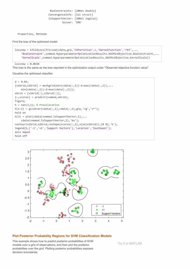
BoxConstraints: [200x1 double] ConvergenceInfo: [1x1 struct] IsSupportVector: [200x1 logical] Solver: 'SMO' Properties, Methods

Find the loss of the optimized model.

lossnew = kfoldLoss(fitcsvm(cdata,grp,'CVPartition',c,'KernelFunction','rbf',... 'BoxConstraint',svmmod.HyperparameterOptimizationResults.XAtMinObjective.BoxConstraint,... 'KernelScale',svmmod.HyperparameterOptimizationResults.XAtMinObjective.KernelScale))

lossnew = 0.0650 This loss is the same as the loss reported in the optimization output under "Observed objective function value".

Visualize the optimized classifier.

d = 0.02; [x1Grid,x2Grid] = meshgrid(min(cdata(:,1)):d:max(cdata(:,1)),... min(cdata(:,2)):d:max(cdata(:,2))); xGrid = [x1Grid(:),x2Grid(:)]; [~,scores] = predict(svmmod,xGrid); figure; h = nan(3,1); % Preallocation h(1:2) = gscatter(cdata(:,1),cdata(:,2),grp,'rg','+*'); hold on h(3) = plot(cdata(svmmod.IsSupportVector,1),... cdata(svmmod.IsSupportVector,2),'ko'); contour(x1Grid,x2Grid,reshape(scores(:,2),size(x1Grid)),[0 0],'k'); legend(h,{'-1','+1','Support Vectors'},'Location','Southeast'); axis equal hold off

Plot Posterior Probability Regions for SVM Classification ModelsThis example shows how to predict posterior probabilities of SVMmodels over a grid of observations, and then plot the posteriorprobabilities over the grid. Plotting posterior probabilities exposesdecision boundaries.

Try it in MATLAB

Load Fisher's iris data set. Train the classifier using the petal lengths and widths, and remove the virginica speciesfrom the data.

load fisheriris classKeep = ~strcmp(species,'virginica'); X = meas(classKeep,3:4); y = species(classKeep);

Train an SVM classifier using the data. It is good practice to specify the order of the classes.

SVMModel = fitcsvm(X,y,'ClassNames',{'setosa','versicolor'});

Estimate the optimal score transformation function.

rng(1); % For reproducibility [SVMModel,ScoreParameters] = fitPosterior(SVMModel);

Warning: Classes are perfectly separated. The optimal score-to-posterior transformation is a step function.

ScoreParameters

ScoreParameters = struct with fields: Type: 'step' LowerBound: -0.8431 UpperBound: 0.6897 PositiveClassProbability: 0.5000

The optimal score transformation function is the step function because the classes are separable. The fieldsLowerBound and UpperBound of ScoreParameters indicate the lower and upper end points of the interval of scorescorresponding to observations within the class-separating hyperplanes (the margin). No training observation fallswithin the margin. If a new score is in the interval, then the software assigns the corresponding observation apositive class posterior probability, i.e., the value in the PositiveClassProbability field of ScoreParameters.

Define a grid of values in the observed predictor space. Predict the posterior probabilities for each instance in thegrid.

xMax = max(X); xMin = min(X); d = 0.01; [x1Grid,x2Grid] = meshgrid(xMin(1):d:xMax(1),xMin(2):d:xMax(2)); [~,PosteriorRegion] = predict(SVMModel,[x1Grid(:),x2Grid(:)]);

Plot the positive class posterior probability region and the training data.

figure; contourf(x1Grid,x2Grid,... reshape(PosteriorRegion(:,2),size(x1Grid,1),size(x1Grid,2))); h = colorbar; h.Label.String = 'P({\it{versicolor}})'; h.YLabel.FontSize = 16; caxis([0 1]); colormap jet; hold on gscatter(X(:,1),X(:,2),y,'mc','.x',[15,10]); sv = X(SVMModel.IsSupportVector,:); plot(sv(:,1),sv(:,2),'yo','MarkerSize',15,'LineWidth',2); axis tight hold off

In two-class learning, if the classes are separable, then there are three regions: one where observations havepositive class posterior probability 0, one where it is 1, and the other where it is the positive class prior probability.

Analyze Images Using Linear Support Vector MachinesThis example shows how to determine which quadrant of an image ashape occupies by training an error-correcting output codes (ECOC)model comprised of linear SVM binary learners. This example alsoillustrates the disk-space consumption of ECOC models that store support vectors, their labels, and the estimated coefficients.

Create the Data Set

Randomly place a circle with radius five in a 50-by-50 image. Make 5000 images. Create a label for each imageindicating the quadrant that the circle occupies. Quadrant 1 is in the upper right, quadrant 2 is in the upper left,quadrant 3 is in the lower left, and quadrant 4 is in the lower right. The predictors are the intensities of each pixel.

d = 50; % Height and width of the images in pixels n = 5e4; % Sample size X = zeros(n,d^2); % Predictor matrix preallocation Y = zeros(n,1); % Label preallocation theta = 0:(1/d):(2*pi); r = 5; % Circle radius rng(1); % For reproducibility for j = 1:n figmat = zeros(d); % Empty image c = datasample((r + 1):(d - r - 1),2); % Random circle center x = r*cos(theta) + c(1); % Make the circle y = r*sin(theta) + c(2); idx = sub2ind([d d],round(y),round(x)); % Convert to linear indexing figmat(idx) = 1; % Draw the circle X(j,:) = figmat(:); % Store the data Y(j) = (c(2) >= floor(d/2)) + 2*(c(2) < floor(d/2)) + ... (c(1) < floor(d/2)) + ... 2*((c(1) >= floor(d/2)) & (c(2) < floor(d/2))); % Determine the quadrantend

Plot an observation.

figure imagesc(figmat)

Try it in MATLAB

α

h = gca; h.YDir = 'normal'; title(sprintf('Quadrant %d',Y(end)))

Train the ECOC Model

Use a 25% holdout sample and specify the training and holdout sample indices.

p = 0.25; CVP = cvpartition(Y,'Holdout',p); % Cross-validation data partition isIdx = training(CVP); % Training sample indices oosIdx = test(CVP); % Test sample indices

Create an SVM template that specifies storing the support vectors of the binary learners. Pass it and the trainingdata to fitcecoc to train the model. Determine the training sample classification error.

t = templateSVM('SaveSupportVectors',true); MdlSV = fitcecoc(X(isIdx,:),Y(isIdx),'Learners',t); isLoss = resubLoss(MdlSV)

isLoss = 0 MdlSV is a trained ClassificationECOC multiclass model. It stores the training data and the support vectors of eachbinary learner. For large data sets, such as those in image analysis, the model can consume a lot of memory.

Determine the amount of disk space that the ECOC model consumes.

infoMdlSV = whos('MdlSV'); mbMdlSV = infoMdlSV.bytes/1.049e6

mbMdlSV = 763.6151 The model consumes 763.6 MB.

Improve Model Efficiency

You can assess out-of-sample performance. You can also assess whether the model has been overfit with acompacted model that does not contain the support vectors, their related parameters, and the training data.

Discard the support vectors and related parameters from the trained ECOC model. Then, discard the training datafrom the resulting model by using compact.

Mdl = discardSupportVectors(MdlSV); CMdl = compact(Mdl); info = whos('Mdl','CMdl');

[bytesCMdl,bytesMdl] = info.bytes; memReduction = 1 - [bytesMdl bytesCMdl]/infoMdlSV.bytes

memReduction = 1×2 0.0626 0.9996

In this case, discarding the support vectors reduces the memory consumption by about 6%. Compacting anddiscarding support vectors reduces the size by about 99.96%.

An alternative way to manage support vectors is to reduce their numbers during training by specifying a larger boxconstraint, such as 100. Though SVM models that use fewer support vectors are more desirable and consume lessmemory, increasing the value of the box constraint tends to increase the training time.

Remove MdlSV and Mdl from the workspace.

clear Mdl MdlSV

Assess Holdout Sample Performance

Calculate the classification error of the holdout sample. Plot a sample of the holdout sample predictions.

oosLoss = loss(CMdl,X(oosIdx,:),Y(oosIdx))

oosLoss = 0

yHat = predict(CMdl,X(oosIdx,:)); nVec = 1:size(X,1); oosIdx = nVec(oosIdx); figure; for j = 1:9 subplot(3,3,j) imagesc(reshape(X(oosIdx(j),:),[d d])) h = gca; h.YDir = 'normal'; title(sprintf('Quadrant: %d',yHat(j))) end text(-1.33*d,4.5*d + 1,'Predictions','FontSize',17)

The model does not misclassify any holdout sample observations.

See Also

••

bayesopt | fitcsvm | kfoldLoss

Related TopicsTrain Support Vector Machines Using Classification Learner AppOptimize a Cross-Validated SVM Classifier Using bayesopt

References[1] Hastie, T., R. Tibshirani, and J. Friedman. The Elements of Statistical Learning, second edition. New York:Springer, 2008.

[2] Christianini, N., and J. Shawe-Taylor. An Introduction to Support Vector Machines and Other Kernel-BasedLearning Methods. Cambridge, UK: Cambridge University Press, 2000.

[3] Fan, R.-E., P.-H. Chen, and C.-J. Lin. “Working set selection using second order information for training supportvector machines.” Journal of Machine Learning Research, Vol 6, 2005, pp. 1889–1918.

[4] Kecman V., T. -M. Huang, and M. Vogt. “Iterative Single Data Algorithm for Training Kernel Machines from HugeData Sets: Theory and Performance.” In Support Vector Machines: Theory and Applications. Edited by Lipo Wang,255–274. Berlin: Springer-Verlag, 2005.