support vector machine for spatial...

Research Article

Support Vector Machine forSpatial Variation

Clio AndrisMassachusetts Institute ofTechnology

David CowenUniversity of South Carolina,Columbia

Jason WittenbachThe Pennsylvania State University

AbstractLarge, multivariate geographic datasets have been used to characterize geographicspace with the help of spatial data mining tools. In our study, we explore the suffi-ciency of the Support Vector Machine (SVM), a popular machine-learning tech-nique for unsupervised classification and clustering, to help recognize hiddenpatterns in a college admissions dataset. Our college admissions dataset holds over10,000 students applying to an undisclosed university during one undisclosed year.Students are qualified almost exclusively by their standardized test scores andschool records, and a known admissions decision is rendered based on these crite-ria. Given that the university has a number of political, social and geographiceconometric factors in its admissions decisions, we use SVM to find implicit spatialpatterns that may favor students from certain geographic regions. We first explorethe characteristics of the applicants in the college admissions case study. Next, weexplain the SVM technique and our unique ‘threshold line’ methodology for bothdiscrete (regional) and continuous (k-neighbors) space. We then analyze the resultsof the regional and k-neighbor tests in order to respond to the methodological andgeographic research questions.

1 Introduction

How to best characterize geographic space, given a large set of geographic descriptors,is an issue that has attracted much attention. While tabular data formats, such as a

Address for correspondence: Clio Andris, Department of Urban Studies and Planning,Massachusetts Institute of Technology, 77 Massachusetts Avenue, Cambridge, MA 02139, USA.Email: [email protected]

bs_bs_banner

Transactions in GIS, 2012, ••(••): ••–••

© 2012 Blackwell Publishing Ltddoi: 10.1111/j.1467-9671.2012.01354.x

spreadsheet, allow some knowledge discovery and sorting, this analysis is not alwayssufficient to visualize and reveal relationships when the number of variables reaches aspecific order of magnitude.

1.1 Pattern Recognition in Spatial Data

In the field of Spatial Statistics, the statistical significance of spatial patterns, geo-graphic adjacency, point patterns, cluster detection can be measured by Moran’s I(Moran 1950) or Geary’s C (Geary 1954), statistics for interaction (Ord 1975), Hot& Cold Spot Detection (Cressie 1992), and LISA (Local Indicators of Spatial Auto-correlation) (Anselin 1995). Also, spatial data mining tools have recently proven to besuccessful in discovering unseen patterns in large, high-dimensional datasets. Thisprocess of Exploratory Data Analysis (EDA) (Tukey 1980) has been approached suc-cessfully through visual data mining (Keim 2002). Applying these paradigms tospatial data, MacEachren and Kraak (1997) initially expressed the needs of Explora-tory Spatial Data Analysis (ESDA). MacEachren et al. (2004) explain that the func-tions of geovisualization are to explore, analyze, synthesize and present, while Guoet al. (2005) add that exploring data should be intuitive, visual and able to supportdecision making. Software such as GeoDA (Anselin et al. 2006) and GeoVISTAStudio (Takatsuka and Gahegan 2002) use interactive selecting and linking and brush-ing (MacEachren and Taylor 1994, Plaisant et al. 1999) to help users find patternsand anomalies.

Other approaches to the problem of finding patterns in high-dimensionalspatial analysis lie in feature reduction methods stemming from the signal processingliterature. These include eigenvector decomposition (Calabrese et al. 2009), formsof principal component analysis and singular value decomposition. Data miningmethods like supervised and unsupervised classification methods, anomaly detec-tion, association rules, and clustering methods (Fayyad et al. 1996, Tan et al. 2006)classify entities based on many features. These geographic problems are shown inapplied research in the work of Miller and Han (2001), and in other work withdecision trees, (Li and Claramunt 2006), rule-based mining (Mennis and Liu 2005),clustering tasks (Jain et al. 1999) and self-organizing maps (Guo et al. 2005). Fewresearchers have used machine learning tools for spatial endeavors, althoughliterature, including the work of Openshaw and Openshaw (1997), supports theirusage.

1.2 Spatial Non-Stationarity

Apart from the issue of high dimensionality, some geographic datasets have implicitelasticities that cannot be described well by dimensionality reduction tools and indices,resulting in a problem of spatial non-stationarity. Spatial non-stationarity is evidencedwhen explanatory variables explain outcomes in only select areas. For example, socialprocesses tend to be non-stationary (e.g. point patterns of disease clusters may arise indifferent areas for different reasons) (Fotheringham et al. 2002).

Processes of non-stationarity and multivariate spatial dependence can be unearthedwith the help of dynamic ESDA environments that link statistical packages with GIS.

2 C Andris, D Cowen and J Wittenbach

© 2012 Blackwell Publishing LtdTransactions in GIS, 2012, ••(••)

Examples include Moran scatterplots (Anselin et al. 2006), multivariate variogramclouds (Cook et al. 1997), and variance-based cross-variograms (Cressie and Wikle1998). Methods such as Bayesian networks and Markov chain/Monte Carlo (MCMC)approaches (Besag and Green 1993) have been known to find important causal/correlated factors of phenomena, given many possible input factors, but have yet tosubstantially integrate into the analysis of spatial-nonstationarity.

Furthermore, statistical techniques need to be applied carefully to variables exhibit-ing spatial dependence (Legendre 1993, Anselin 2002). In traditional regression, staticvariable coefficients universally describe variable relationships across space. Conversely,the study of spatial non-stationarity has allowed for statistical methods that reportchanges in coefficient values as well as parameter values themselves (Foody 2004). Yetthe underlying mechanisms behind spatial non-stationarity often include an exchange ofspatial parameter estimates of independent and dependent variables. Here, the cause ofan observed phenomenon is difficult to untangle, due not only to many candidate causalvariables, but also to the combination of causal variables being the actual cause. The‘recipe’ for the combination of these variables (e.g. variable elasticities) can be exploredwith the help of tools, most notably geographically weighted regression (GWR)(Brunsdon et al. 1996, 1998; Fotheringham et al. 2002). GWR gives insight into howparameter coefficients change over geographic space in order to explain a (changing)dependent variable.

1.3 Introducing the Support Vector Machine

Our experimental tool, the Support Vector Machine (SVM), improves on GWR in ourcase, as we have a binary dependent variable, a feature in which SVM specializes, whileGWR and regression methods excel in analyzing numerical values as dependent vari-ables. To clarify, the dependent variable can be a predicted (i.e. expected) output fromwhich to compare the actual output (such as in OLS Regression) or as an output that isused to retrofit dependent variable coefficients (such as in GWR). Also, our case exhib-its a linear ‘exchange’ between independent variables, (e.g. the unique combination oftwo or more parameters) which is captured well with the SVM discriminant lines, butwould not be captured as well with two independent parameter coefficients. (Note thatthis parameter ‘exchange’ is different from parameter co-linearity). Along the samelines, it is not important which independent variable is playing a more significant role inthe outcome (which is often a significant source of power for GWR), but that it is theimplicit combination of parameters that affects the binary decision. Therefore, wechoose the SVM to improve on the capabilities of GWR under these circumstances.

The output of the SVM (or a similar linear discriminant) is a decision line thatdescribes the relationships between input variables, as well as their leniency or strin-gency on the outcome decision. Meanwhile, the slope of the discriminant line for eachtrained region can reveal whether one variable is adding more weight to the value of thebinary decision. Using the SVM in a spatially-varying context may enhance the toolsetof those with similar spatial dependency datasets, wherein an inter-dependent variablerelationship is at play as well.

With this reasoning at hand, we further explore the sufficiency of SVM in unearth-ing the geographic changes in dependent variables, and combinations of these variables,that predict how the admissions decision process may be inconsistent over geographicspace. SVM is most typically considered a predictive tool in the data mining and

Support Vector Machine for Spatial Variation 3


pattern recognition literature, but here we use its initial training outcome as a lineardiscriminant to describe the geographic ‘biases’ of admitting college students based ontheir application scores. SVM is a machine-learning technique that is a popular methodfor data mining tasks in classification. (Cortes and Vapnik 1995) This research repre-sents one of the first examples of test to evaluate SVM’s applicability to a spatialproblem, as the literature that uses SVM for a geographic problem is limited and incon-clusive (Kanevski et al. 2002).

1.4 Experiment

To empirically test the use of SVM for investigating geographic patterns, we use a casestudy test of geographic differences in college admissions standards with regard toapplicant qualifications. A college admissions dataset for a large university is used, inwhich over 10,000 students applied to the university during one undisclosed admissionscycle year. Although SVM’s utility often lies in its ability to take many variables (i.e.features) into account, we use only two in order to qualify a student for admission: astudent’s grade point average (GPA) and standardized test scores (SAT or ACT), asthese two quantitative variables alone account for over 95% of admissions decisions atthe university – which is not atypical of admissions office practice in large universities(Horn and Flores 2003, Hawkins and Clinedinst 2006). Each applicant is geo-locatedby his or her application ZIP code.

The article proceeds as follows: We first explore the characteristics of the applicantsin the college admissions case study and some possible reasons why there might be atopological inconsistency in the threshold pattern results. Next, we explain the SVMtechnique, the process with which we qualify its utility for our dataset, how we createthreshold lines and respond to the socio-geographic research question on college admis-sions. We then share the results of our analysis of both discrete and continuous (inter-polated) space. We conclude with a brief discussion and propose a few larger researchquestions.

2 The Case Study Question and Dataset

As mentioned, a large university provided us with a large dataset of applicants for oneundisclosed year of traditional fall semester admissions. After removing non-traditionalapplicants (e.g. transfer students), 10,887 remaining applicants are geographically iden-tified by U.S. ZIP code.

2.1 Applicant Qualifications

Undergraduate applicants are evaluated by SAT and GPA. Colloquially, GPA typicallyrepresents a student’s achievement in school, and SAT represents a student’s capacity tothink logically and methodically; a student can be considered accomplished by eithermeasure. The applicants’ average SAT is 1129 (1) (a comparable national average forthe admissions year is 1030, College Board 2007) and average GPA is 3.49. Of theseapplicants, 8,716 (80%) are accepted, and 3,660 (42% of accepted) enrolled in theuniversity.



2.2 Geography of Applicants

The point-density of applicants varies significantly over geographic space. Nine differ-ent ZIP codes, each in South Carolina, produced between 100 and 200 applicants. Themajority of U.S. ZIP codes did not produce an applicant, and over 500 ZIP codes pro-duced a single applicant (Figure 1). The geographic distribution of the applicants showsthe majority of ZIP codes producing applicants in South Carolina, and significant activ-ity in the northeast corridor, mid western cities, Atlanta, Georgia, and Charlotte, NorthCarolina (Figure 2).

In order to better manage the diverse levels of applicant density, we divide theapplicants into 12 regions, by iterating between minimizing the range between regionalnumber of applicants, maintaining census divisions, and following regional associa-tions. To represent the large volume of South Carolina applicants, three regions: Mid-lands (containing Columbia), Lowcountry (containing Charleston and Myrtle Beach)and Upstate (containing Greenville-Spartanburg) were derived from area code bounda-ries altered to align with county boundaries. Three regions are considered “neighborstates”, five are considered to be an “inner ring” or “outer ring”, and one is consideredto be a “far region.” (Figure 3). The final result is 12 regions, with applicant cardinalityranging from 215 to 2,879. (Table 1)

Studying average SAT, GPA and percent accepted from each region providesa graphical synthesis of the premise of this study (Figure 4). The data sparks somecuriosity, as regions like North Carolina and the South have higher acceptance ratesthan Appalachia, although the average scores are lower. The graph also shows thatSouth Carolina regions have lower average SAT values, but still boast relatively highadmissions rates. This may seem puzzling, but we cannot secure a bias, as theseresults decouple the applicant’s criteria from the admissions decision in the process ofaggregate averaging. With consideration of disaggregation and uncertainty in alloca-tion problems in spatial decision support systems (Fotheringham et al. 1995, Aertset al. 2003) we seek out a linear discriminant to sidestep averaging and provide amore accurate representation of the biases or regional preferences in the data set.

Figure 1 A log-linear frequency plot of applicants per U.S. ZIP code shows that themajority of ZIP codes produced few or no applicants, while some produced almost 200applicants



2.3 Competing Hypotheses of Geographic Affirmative Action

The notion of geographic affirmative action proposes that one locale or purportedaddress may entitle him or her to benefits or blockades to admissions. In our experi-ence, we find one school, Hastings Law School in San Francisco, that openly claims toprescribe to affirmative action based on geography, as a student’s hometown can reflecta student’s access to opportunities and economic factors.

Our prediction for the outcome of these admissions thresholds is not necessarilyclear, because there are competing interests involved. Often, large universities arefunded in some way by taxpayers, and local residents without the highest qualificationsexpect admission to the school that is nearby and is the recipient of their tax dollars.

Conversely, it is in the university’s best interest to admit the most qualified stu-dents. Also, in some schools, there may be a difference in tuition depending on fromwhere the student hails (usually in-state or out-of-state) (Marble 1997). We may not beAble to understand the university’s strategy or potential bias, as much is hidden to us,but we may be able to illuminate some spatial patterns in their decisions. Next, weexplain our implementation of the SVM method and our treatment of this method toquantify variations of admissions thresholds in our case study.

Figure 2 The geographic distribution of places that yield applicants (as denoted bya ZIP code centroid), is heavily biased towards the Northeast Corridor and SouthCarolina. Note that number of applicants per ZIP code is not shown here, e.g. a ZIPcode that produces 100 or 1 applicant(s) is graphically identical



Figure 3 Twelve study regions are created, where each will be tested as a singularentity using the SVM tool

Table 1 Applicant summary variables by region

Region Area (States) Applicants Mean SAT Mean GPA % Accepted

South CarolinaLowcountry 1/3 1878 1081 3.41 74.23Midlands 1/3 2879 1101 3.45 77.56Upstate 1/3 1647 1104 3.56 81.78Neighbor StatesGeorgia 1 593 1181 3.59 86.17North Carolina 1 612 1185 3.71 90.36Virginia 1 526 1166 3.32 83.84Near RegionsAppalachian 3 215 1218 3.88 88.84Middle Atlantic 4* 862 1171 3.46 80.74South 4 228 1179 3.64 89.91Far RegionsMidwest 5 506 1200 3.62 85.97New England 7 519 1149 3.36 74.37West 21 282 1216 3.67 83.68



3 Method

Now that we have reviewed motivations, we next explain how patterns can be eluci-dated. Since the applicant’s test scores and school performance are quantitative and theclassifier (admitted / rejected) is binary, this dataset is well suited for tools that producea linear discriminant (Figure 5). The challenge is to find the dividing line for eachregion, and then compare the lines to find the regions that have a higher or lower stand-ard of admissions. Different regional thresholds may admit students that would berejected if from another region.

We use classic Linear Discriminant Analysis (LDA) as a ‘control’, since it is a moretraditional method that has been used previously for geographic endeavors, and test itsutility in providing reliable admissions thresholds against the newer, more experimentalSVM. We explain these methods in greater detail below.

3.1 Linear Discriminant Analysis

Linear discriminant functions (Fisher 1938) categorize entities into two (or more)groups based on their features. Today, it is a popular method of classification, used

Figure 4 Mean SAT score and mean GPA for students in each region are comple-mented by percentage of students accepted. Notably, the percentage of studentsaccepted may not scale with the credentials of the regional applicants



in the fields of artificial intelligence, machine training, economics, biostatistics anddata mining. In linear discriminant analysis (LDA), a linear combination of variablesclassifies an observed item into one of two classes (Ladd 1966). LDA attempts to drawa decision region between classes that tries to seperate clusters as much as possible infeature space (Balakrishnama and Ganapathiraju 1999). Since it has been widelyaccepted and used often in academic literature (Shawe-Taylor and Christianini 2000), itis chosen as a ‘control’ method against which to test how accurately the SVM correctlyclassifies entities.

3.2 Support Vector Machine

SVM has gained notoriety for its success in unsupervised classification. Its applica-tions are diverse: face detection (Osuna et al. 1997), text classification (Chen 2005),financial prediction (Kim 2003), biology (Noble 2006) and document retrieval, filter-ing and categorization (Li and Shawe-Taylor 2003). SVM has been praised as a cross-section of “geometric intuition, elegant mathematics, theoretical guarantees, andpractical algorithms” (Bennett and Campbell 2002). The application of SVM to geo-graphic problems is quite limited, but has been used to classify soil types (Kanevskiet al. 2002).

Duda et al. (2001) define the fundamentals: a linear discriminant function dividesfeature space by a hyperplane decision surface, and the decision boundary is notunique, as many boundaries can split a dataset into two or more classes. The SVMthen iterates and ‘learns’ to classify observations in one of two classes, and creates adecision boundary that spaces itself as far as possible (in geometric feature space) fromrecords.

The SVM finds the largest margin that separates the data into distinct classes andwhose geometric bisector (called a hyperplane) can be considered a discriminant bound-ary. When the data is linearly separable, the margin for any tentative discriminatinghyperplane is defined as the perpendicular distance between the nearest points on eitherside of the hyperplane. Let the variable w be some vector that defines a collection of

Figure 5 Binary discriminant lines separate admitted and rejected students on a2-variable plot



hyperplanes perpendicular to it. Equation (3) shows three such examples (x is an inputvector and b is an offset). With a proper scaling of w and b, these three equations rep-resent the decision boundary (where f(x) = 0), and the parallel boundaries of themargin, on which lie the nearest events on either side of the decision boundary (wheref(x) = +1 and -1). With this setup, the size of the margin is given by Equation (2).Events are not always correctly separated and do not lie inside the margin is given byEquation (3). Thus, the maximum margin hyperplane (MMH) is found by minimizingthe norm of w with respect to the classification constraint (Tan et al. 2006).

� � � � � �w x b w x b w x b• + = − • + = + • + =1 1 0 (1)

Margin = 22�

w(2)

f xw x b

w x b( )�

� �� = • + ≥

− • + ≤ −{ 1 11 1

ifif

(3)

In a linearly-separable case, the MMH is designed to disallow data points fromfalling inside it, amounting to vectors only on the margin (and beyond). Since theadmissions data is not linearly separable (indicating that some applicants are evaluatedon more than SAT and GPA but additional criteria such as essays, recommendations, orclass rank) ‘slack variables’ are introduced, where a new objective function (Equation4) is also subject to constraints (Equation 5), where xi is the slack variable or errorterm. We invite the reader to explore this in detail in Tan et al. (2006) and Cortes andVapnik (1995).

L ww

C ik

i

N

( ) = + ⎛⎝⎜

⎞⎠⎟=

∑� 2

12ξ (4)

f xw x b

w x bii i

i i( )�

� �� = • + ≥ −

− • + ≤ − +{ 1 11 1

ifif

ξξ (5)

Our implementation and use of these tools is explained below.

3.3 Implementation

LDA is implemented in SPSS version 15.0 (SPSS 2006). Canonical linear discriminantcoefficients for the SAT variable, GPA variable and a constant were used to find thedecision lines from the format: 0 = y (coefficient) + x (coefficient) + constant. In align-ment with SVM notation, the coefficients are considered variable weights wi. Forregional and neighborhood analysis, we use SVM methods (“svmtrain” and “svmclas-sify”) from the bioinformatics toolbox in MATLAB (The Mathworks 2003–2011) and



the support vector machine tool from the RapidMiner Environment (Mierswa et al.2006).

3.4 Test for Prediction Accuracy

To determine whether the SVM is well-suited for this type of discriminant analysis, wetest the prediction accuracy of LDA and SVM, as we know the actual decisions of theschool, and can compare these to the predicted values. We used the popular Chi-Squared test to assess contingency of false accepts, true accepts, false rejects and truerejects (Equation 6) (Blalock 1960):

χ22

= −( )∑ f ff

o e

e

(6)

where fo is the observed value of a cell in the contingency matrix and fe is the calculatedexpected value of the cell if the distribution was absolute.

3.5 Divisions for Geographic Grouping

As our question is geographic in nature, we group applicants (as points for the LDAand SVM analysis) by similar location. We take advantage of both discrete (regional)geography described in Section 2.2, and continuous geography.

Regions

In terms of the regional geography, the SVM and LDA are employed on sets of appli-cants in groups of 12 cohesive regions. (Figure 3) As mentioned, these regions arecreated to help explore the applicants’ geography. We train the SVM 100 times tooutput a linear threshold for each individual region and use the average of the thresholdresults, in order to avoid anomalies and overfitting.

K-Neighbors

In addition to regional variation, we also create a smooth surface that allows for amore detailed view of the geographic change in threshold values. We assign each appli-cant to a random place within his or her ZIP code boundary. We then group the appli-cant with his or her nearest 99 Euclidean neighbors and use this subset to the lineardiscriminant LDA or SVM method. We then assign the discriminant line’s threshold asthe threshold at the applicant’s location. Because of the vast differences in applicantdensity, some groups will have all 99 neighbors within the same ZIP code, while otherswill span over 1,000 miles. For this analysis, we only include applicants from the 48contiguous U.S.

3.6 Method for Comparing Thresholds

In order to quantify and compare the lines, we normalize the SAT and GPA variablesto a 0-1 scale and integrate the lines within the normalized 10 x 10 feature space



boundary. In practice, a high threshold line will leave a more significant geometric areabeneath it, which we use to represent the stringency of the threshold. We also note thatthe original lines are useful for describing the regions, as steep slope indicates that GPA(x axis value) may affect the admissions decision more than SAT, and vice versa.

After reviewing the steps of our process, we now discuss the results of the methods’accuracy and the results of the regional test and k-neighbor test.

4 Results

The graphical nature of the SVM (and LDA for comparison) output enables a visualanalysis where we can see that some regions divide the point cloud of applicants insimilar ways, like the South and North Carolina, or very different ways like the Upstateand the West (Figure 6). This chart indicates that with 95% accuracy, a student withthe same SAT and GPA credentials might be rejected depending on his or her region of

Figure 6 SVM (solid line) and LDA (dashed line) discriminant lines lie on a scatter plotof GPA and SAT Variables. A point cloud is included behind the discriminant lines toshow the trend of the data events



origin. A student with a 900 SAT and 3.75 GPA would probably be accepted if he orshe is a resident of South Carolina or Virginia, but not of the West. And points (akaapplicants) in Figure 6 that lie between two SVM threshold lines are subject to such apredicament. The following discussion will help us put these lines into quantitativecontext.

4.1 Accuracy

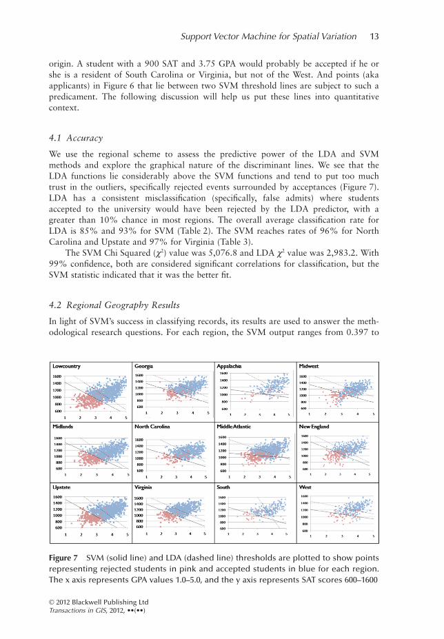
We use the regional scheme to assess the predictive power of the LDA and SVMmethods and explore the graphical nature of the discriminant lines. We see that theLDA functions lie considerably above the SVM functions and tend to put too muchtrust in the outliers, specifically rejected events surrounded by acceptances (Figure 7).LDA has a consistent misclassification (specifically, false admits) where studentsaccepted to the university would have been rejected by the LDA predictor, with agreater than 10% chance in most regions. The overall average classification rate forLDA is 85% and 93% for SVM (Table 2). The SVM reaches rates of 96% for NorthCarolina and Upstate and 97% for Virginia (Table 3).

The SVM Chi Squared (c2) value was 5,076.8 and LDA c2 value was 2,983.2. With99% confidence, both are considered significant correlations for classification, but theSVM statistic indicated that it was the better fit.

4.2 Regional Geography Results

In light of SVM’s success in classifying records, its results are used to answer the meth-odological research questions. For each region, the SVM output ranges from 0.397 to

Figure 7 SVM (solid line) and LDA (dashed line) thresholds are plotted to show pointsrepresenting rejected students in pink and accepted students in blue for each region.The x axis represents GPA values 1.0–5.0, and the y axis represents SAT scores 600–1600



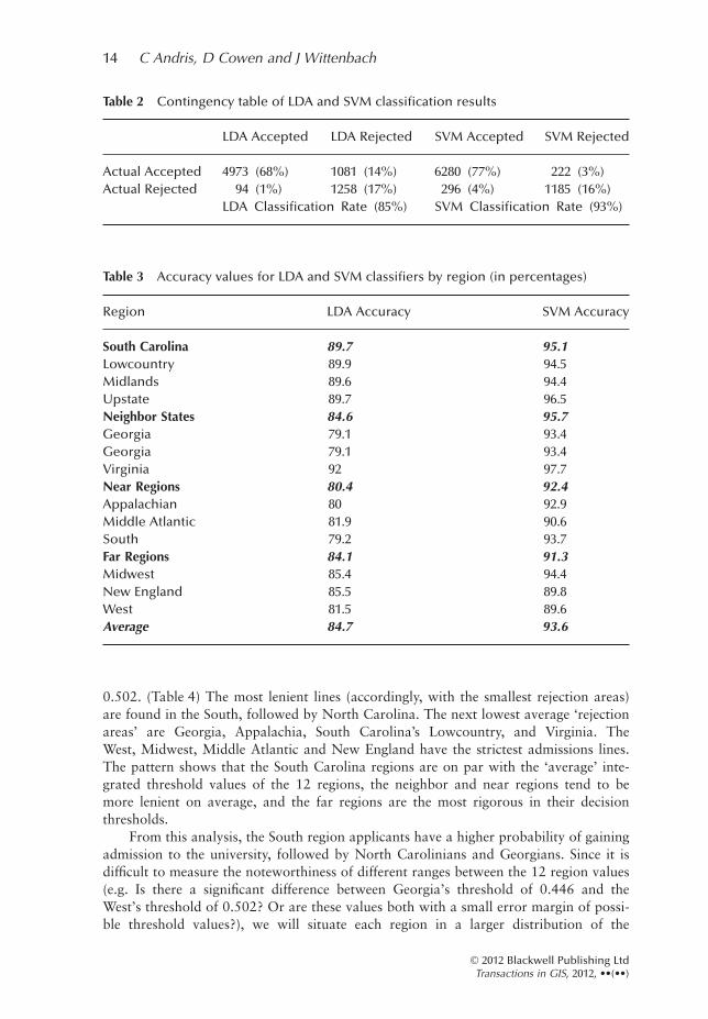
0.502. (Table 4) The most lenient lines (accordingly, with the smallest rejection areas)are found in the South, followed by North Carolina. The next lowest average ‘rejectionareas’ are Georgia, Appalachia, South Carolina’s Lowcountry, and Virginia. TheWest, Midwest, Middle Atlantic and New England have the strictest admissions lines.The pattern shows that the South Carolina regions are on par with the ‘average’ inte-grated threshold values of the 12 regions, the neighbor and near regions tend to bemore lenient on average, and the far regions are the most rigorous in their decisionthresholds.

From this analysis, the South region applicants have a higher probability of gainingadmission to the university, followed by North Carolinians and Georgians. Since it isdifficult to measure the noteworthiness of different ranges between the 12 region values(e.g. Is there a significant difference between Georgia’s threshold of 0.446 and theWest’s threshold of 0.502? Or are these values both with a small error margin of possi-ble threshold values?), we will situate each region in a larger distribution of the

Table 2 Contingency table of LDA and SVM classification results

LDA Accepted LDA Rejected SVM Accepted SVM Rejected

Actual Accepted 4973 (68%) 1081 (14%) 6280 (77%) 222 (3%)Actual Rejected 94 (1%) 1258 (17%) 296 (4%) 1185 (16%)

LDA Classification Rate (85%) SVM Classification Rate (93%)

Table 3 Accuracy values for LDA and SVM classifiers by region (in percentages)

Region LDA Accuracy SVM Accuracy

South Carolina 89.7 95.1Lowcountry 89.9 94.5Midlands 89.6 94.4Upstate 89.7 96.5Neighbor States 84.6 95.7Georgia 79.1 93.4Georgia 79.1 93.4Virginia 92 97.7Near Regions 80.4 92.4Appalachian 80 92.9Middle Atlantic 81.9 90.6South 79.2 93.7Far Regions 84.1 91.3Midwest 85.4 94.4New England 85.5 89.8West 81.5 89.6Average 84.7 93.6



(10,000+) k-neighbor threshold values. We now explore the results of the 99k-neighbors, a more disaggregate analysis where each applicant location is given itsown threshold.

4.3 K-Neighbors and Interpolation Results

For each of the 10,000 plus records created (by training groups of each applicant withhis or her 99 nearest neighbor applicants), the SVM correctly classifies 96% (with astandard deviation of 3.1), with a minimum classification rate of 83% and maximum of100% when training the geographically-clustered groups of 100 applicants, the latter ofwhich is found frequently. (In fact, over 20% of training groups had a classificationaccuracy of over 99%). From these rates, we can see that more granular spatial analysisscopes (99 neighbors versus a ‘region’) are unearthing the phenomenon of clear ‘micro-region’ decisions.

The mean threshold value for k-neighbor decisions is 0.454 (normally distributedwith s.d. 0.034). Given this distribution, each of the 12 regions above fall within onestandard deviation of the mean, except for the South (two standard deviations belowthe mean) and each of the Far Regions (each at 1.5 standard deviations above themean). Statistically, these results indicate that the majority of the 12 regions are foundroughly within the 16th to 84th percentiles of all thresholds. Yet the three far regions areat the 88th, 95th and 95th percentiles of the dataset and the South is near the 5th percen-tile, indicating the significant deviance of these regions from expectation (i.e. the meanof 0.454). Below, we show the results of the k-neighbor analysis.

Table 4 Normalized area under the SVM discriminantline for each region

RegionNormalized Area UnderSVM Line

South Carolina .460Lowcountry 0.448Midlands 0.473Upstate 0.461Neighbor States .440Georgia 0.446North Carolina 0.425Virginia 0.448Near Regions .442Appalachian 0.447Middle Atlantic 0.484South 0.397Far Regions .499Midwest 0.493New England 0.502West 0.502Average .460



In the k-neighbors analysis, the maximum threshold value is 0.537, found on theWest Coast, and minimum is 0.222, found in suburbs north of Baltimore. Results of anIDW interpolated surface show a more refined picture as the data is not clustered byregions, and statistics can transcend state (or sub-state) boundaries (Figure 8). It seemsas though applicants from Alabama, East Mississippi, Southern Florida, Virginia orMiddle Tennessee are more likely to gain admission than other applicants with the samecredentials hailing from other places. Similar to the regional results, we see that thosefrom the West Coast are held to higher standards. Furthermore, pockets of high-standards arise in the Chicago area, Ohio cities, New Jersey, New York and parts ofNew England, including Boston (Figure 9). When comparing these areas with theirneighbors, we find students hailing from these areas are subject to higher thresholdsthan those from Pittsburgh, Pennsylvania; Long Island, New York; Detroit, Michigan;and Rhode Island, and are held to much higher standards than students from Virginia.We also note a curious oasis of admissions leniency in Maryland into southern Pennsyl-vania (Figure 10).

The most geographically-clustered variation in admissions thresholds occurs inSouth Carolina, where applicants from the downtown parts of some of South Caroli-na’s major cities: Columbia, Charleston, Myrtle Beach and Hilton Head, seem to avoidthe higher standards of the suburbs that begin adjacent to the downtown (Figure 11).Conversely, the large metropolitan area Greenville-Spartanburg shows that thres-holds alleviate outside the city, particularly to the south. Especially in the cases ofColumbia and Greenville-Spartanburg, it seems clear that different neighborhoods

Figure 8 A moving window interpolation of the 100-neighborhood zone SVM traininggives a more detailed view of thresholds



(and neighborhood high schools) produce students that are regarded differently in theeyes of this university’s admissions office.

Moreover, applicants from Charlotte, North Carolina (and Atlanta, Georgia,although out of scope but visible in Figure 8) and less so Georgia cities Savannah andAugusta, are given lower thresholds than those directly inside the state line. Charlotte’svalues are among the lowest in the U.S., while some of the most stringent thresholds arefound within miles of Charlotte, but within South Carolina.

4.4 Results in Context

Although we previously visited the threshold values from the 12 regions in context inthe k-neighbor distribution, we are still left with the challenge of determining the sig-nificance between differences in k-neighbor threshold values, as we yet have no ‘global’(or aspatial) sample of admissions thresholds from which to draw.

To situate both the 12-regional and k-neighbor threshold values and intervals in a‘universal’ range of thresholds, we bootstrap the existing dataset to create a new distri-bution of thresholds. For 10,000 trials, we randomly select 100 applicants from allapplicants and train the SVM to output a new randomized decision threshold line.Notably, the randomized distribution does not account for the geographic locale ofeach applicant, and so we consider this distribution a control from which to test thegeographically-grouped threshold values from the regional and k-neighbor analyses.

Figure 9 The 100-neighbor zone SVM results show threshold variations in the North-east and Midwest. Note that each applicant is assigned to a random place within his orher ZIP code boundary



The mean of the aspatial (randomized) distribution is 0.453 (normally distributedwith s.d. 0.022) compared with mean 0.454 of the spatialized k-neighbor training(s.d 0.033). Sample means of the randomized and k-neighbor distributions are quitesimilar, but the standard deviation is higher for the spatialized distribution. To quantifythe difference between these distributions, and therefore isolate the effect of geography,we conducted an unpaired t-test from samples from each population (see Ruxton2006). Our null hypothesis H0 is that there is no significant difference in these distribu-tions. Our competing hypothesis H1 is that there is a significant difference in the distri-butions. The derived critical value is 2.573, which surpasses H1’s critical value of 1.960(confidence level: 95%), evidencing a significant difference in the distributions. Since themean values are comparable, we focus on the larger standard deviation, which is anindicator of significantly more variation in the types of decisions that are made with thespatially-sorted groups.

Furthermore, while training the randomized applicants, the SVM finds more diffi-culty applying a clear rule to the group. The average SVM training accuracy wasslightly higher for the geographically-grouped values (95.9%) than for the randomly-grouped values (94.5%). Qualitatively, the higher accuracy indicates that training theSVM with geographically-grouped sets results in more reliable decision boundaries, or,restated, in similar geographies, applicants are evaluated with a clearer (set of) rule(s).

In summary, we find that there are geographic variations in the stringencies of theadmissions threshold lines at the regional and city level, even down to the neighbor-hood level in the context of the New York Metropolitan Area and South Carolina and

Figure 10 SVM threshold values for Maryland and vicinity show a pocket of leniency inthe Baltimore suburbs that is not apparent in Washington, D.C.



vicinity. Next, we discuss some of the hypotheses driving these patterns and concludeour study.

5 Discussion

In the prior section, we note geographic variation between admissions thresholds. Wecannot explain with certainty why such difference may be occurring, but we were madeaware of some strategic admissions recruiting factors through personal correspondencewith admissions officers from the undisclosed university. Our results show that onehypothesis for variations in admissions thresholds may be that for lenient areas such asBaltimore, the university wants to draw students from more diverse, underrepresentedlocations. Another, perhaps complementary, theory is that students from particular highschools are more likely to enroll in the university because they have older friends or sib-lings who attend(ed) the university. Following the ideas of social ‘trip chaining’, manytimes word-of-mouth or experience (like visiting the sibling or friend) has a profoundeffect on an applicant’s decision to attend a university. This familiarity can reduce thesocial distance (Andris 2011) to the university although he or she may be geographi-cally further away. According to admissions officers at our university, mentioningformer and current students who are from similar locales as potential applicants is a

Figure 11 The most variation over geographic space occurs in South Carolina, whereapplicants from Charlotte and less so Savannah, are given low thresholds, and down-town parts of South Carolina’s major cities seem sheltered from the standards of thesuburban and exurban areas



helpful tactic for drawing new applicants. Loosening admissions rigidity to studentswho are likely to enroll could save the admissions office time and money for recruiting,and could build momentum relatively easily to widen the channels between ‘loyal’ ZIPcodes and the university enough to start attracting higher caliber students. Although wegain some insight into possible mechanisms behind certain admissions choices, there aredeeper ethical, financial and social issues in college admissions with which we do notengage in this article.

In response to the methodological issue posed in this work, we recall that methodsof quantifying spatial non-stationarity such as Geographically Weighted Regression(GWR), could have also been employed. GWR would have told us perhaps the impor-tance of the GPA or SAT values in admitting a student for each region through itsparameterization method. It would have also given us an error value to understand howwell these variables could predict the outcome. However, this method may not haveaccounted as well for the combination of these variables, e.g. that a low GPA and ahigh SAT help exceedingly more than a high GPA and low SAT. The geometric natureof the SVM makes this exchange clearer. Additionally, a method such as GWR wouldbe helpful if considering continuous-variable outcomes, (e.g. how many cancer deathsresult from an independent variable, such as levels of toxic chemicals in waterresources) but since our case study’s dependent variable is binary (admitted or rejected),the SVM can give us a unqiue threshold line that shows the econometric exchange or‘trade off’ of each variable in contributing to the outcome. Also, SVM will have a non-trivial advantage over other methods of quantifying spatial non-stationary when thespatial data are high-dimensional (e.g. 50+ predictor variables).

6 Conclusions

In summary, the objective of this study is to attempt to evaluate SVM based on itsability to provide an improved method of discerning implicit patterns in a collegeadmissions data set that may favor students from certain geographic regions. Harken-ing back to our introduction, we were confronted with the problem of changingdependent and independent variables in space, and a large dataset that perhaps calledfor help from a new data mining method.

The questions driving this study are twofold. First, we attempt to use a new toolfor geographic analysis. The accuracy measurements indicate that the SVM was a bettertool than linear discriminant analysis (LDA) to use for this study, and its findings showthat with distance, acceptance thresholds become stricter. This method was robust to ageographic dataset that varied significantly in the density of applicants per ZIP code,and did not rely on averages or aggregate data to determine whether all applicants wereevaluated for admissions with the same rules. SVM’s efficiency, accuracy and ability tosynthesize an econometric-type dataset renders it attractive and applicable to other geo-graphic studies. Secondly, we gained insight into whether our university has an implicitgeographic bias or preference when accepting students. Regional analysis shows thatstudents from Virginia and North Carolina regions have the most forgiving thresholdlines, with the pockets of leniency near Baltimore, Charlotte, for example. The mostrigorous threshold lines are in the West, followed by the Midwest and New England.More local trends in South Carolina also show urban/suburban variation.

These numbers may not be enough to vindicate the presence of geographic affirma-tive action and assume that the university has a clear bias towards students hailing from



certain regions. However, with the preliminary conclusions, geographic variance ispresent and the SVM method was successful in discerning this pattern.

Acknowledgements

We are thankful for the comments of Drs. Sarah Battersby, Michael Hodgson andDiansheng Guo. This work was funded in part by the National Defense Science andEngineering Graduate (NDSEG) Fellowship under the Army Research Office (ARO).

Note

1 The data for the study was used with SAT scores from the 1600 point scale. Also, nearly 40%of applicants submitted another popular standardized test, the ACT, in such case this numberwas converted to SAT (College Board 2007) and supplanted only if higher.

References

Aerts J, Goodchild M F, and Heuvelink G M 2003 Accounting for spatial uncertainty in optimi-zation with spatial decision support systems. Transactions in GIS 7: 211–30

Andris C 2011 Metrics and Methods for Social Distance. Unpublished Ph.D. Dissertation, Massa-chusetts Institute of Technology

Anselin L 1995 Local indicators of spatial autocorrelation: LISA. Geographical Analysis 27:93–115

Anselin L 2002 Under the hood: Issues in the specification and interpretation of spatial regressionmodels. Agricultural Economics 27: 247–67

Anselin L, Syabri I, and Kho Y 2006 GeoDA: An introduction to spatial data analysis. Geographi-cal Analysis 38: 5–22

Balakrishnama S and Ganapathiraju A 1999 Linear discriminant analysis: A brief tutorial adden-dum to linear discriminant analysis for signal processing problems. In Proceedings of theSoutheastcon ’99 Conference, Lexington, Kentucky: 78–81

Bennett K and Campbell C 2002 Support Vector Machines: Hype or hallelujah? ACM SIGKKDExplorations 2: 1–13

Besag J and Green P 1993 Spatial statistics and Bayesian computation. Journal of the Royal Sta-tistical Society Series B 55: 25–37

Blalock H M 1960 Social Statistics. New York, McGraw-HillBrunsdon C, Fotheringham A S, and Charlton M 1996 Geographically weighted regression:

A method for exploring spatial nonstationarity. Geographical Analysis 28: 281–98Brunsdon C, Fotheringham A S, and Charlton M 1998 Geographically weighted regression.

The Statistician 47: 431–43Calabrese F, Reades J, and Ratti C 2009 Eigenplaces: Segmenting space through digital signatures.

IEEE Pervasive Computing 9: 78–84Chen P 2005 A tutorial on V-support vector machines. Applied Stochastic Models in Business and

Industry 21: 111–36College Board 2007 About the SAT. WWW document, http://www.collegeboard.comCook D, Symanzik J, Majure J J, and Cressie N 1997 Dynamic graphics in a GIS: More examples

using linked software. Computers and Geosciences 23: 371–85Cortes C and Vapnik V 1995 Support-vector networks. Machine Learning 20: 273–97Cressie N 1992 Statistics for spatial data. Terra Nova 4: 613–17Cressie N and Wikle C 1998 The variance-based cross-variogram: You can add apples and

oranges. Mathematical Geology 30: 789–99



Duda R, Hart P, and Stork D 2001 Pattern Classification (Second Edition). New York, JohnWiley and Sons

Fayyad U, Piatetsky-Shapiro G, and Smyth P 1996 From data mining to knowledge discoveryin databases. AI Magazine 17: 37–54

Fisher R A 1938 The statistical utilization of multiple measurements. Annals of Eugenics 8:376–78

Foody G 2004 Spatial nonstationarity and scale-dependency in the relationship between speciesrichness and environmental determinants for the sub-Saharan endemic avifauna. GlobalEcology and Biogeography 13: 315–20

Fotheringham A S, Densham P, and Curtis A 1995 The zone definition problem in location-allocation modeling. Geographical Analysis 27: 60–77

Fotheringham A S, Brundson C, and Charlton M 2002 Geographically Weighted Regression:The analysis for spatially varying relationships. New York, John Wiley and Sons

Geary R 1954 The contiguity ratio and statistical mapping. The Incorporated Statistician 5:115–46

Guo D, Gahegan M, MacEachren A, and Zhou B 2005 Multivariate analysis and geovisualizationwith an integrated geographic knowledge discovery approach. Cartography and GeographicInformation Science 32: 113–32

Hawkins D and Clinedinst M 2006 State of College Admission. Washington D.C., NACAC(available at http://www.nacacnet.org)

Horn C and Flores S 2003 Percent Plans in College Admissions: A Comparative Analysis of ThreeStates’ Experiences. Cambridge, MA, The Civil Rights Project at Harvard University

Jain A K, Murty M N, and Flynn P J 1999 Data clustering: A review. ACM Computing Surveys31: 264–323

Kanevski M, Pozdnukhov A, Maignan M, and Canu S 2002 Advanced spatial data analysisand modelling with support vector machines. IDIAP Research Report 4: 606–16

Keim D A 2002 Information visualization and visual data mining. IEEE Transactions onVisualization and Computer Graphics 7: 1–8

Kim K 2003 Financial time series forecasting using support vector machines. Neurocomputing 55:307–19

Ladd G 1966 Linear probability functions and discriminant functions. Econometrica 34: 873–85

Legendre P 1993 Spatial autocorrelation: Problem or new paradigm? Ecology 74: 1659–73Li X and Claramunt C 2006 A spatial entropy-based decision tree for classification of geographi-

cal information. Transactions in GIS 10: 451–67Li Y and Shawe-Taylor J 2003 The SVM with uneven margins and Chinese document categoriza-

tion. In Proceedings of the Seventeenth Pacific Asia Conference on Language, Informationand Computation (PACLIC17), Singapore: 216–27

MacEachren A and Taylor D 1994 Visualization in Modern Cartography. Oxford, PergamonMacEachren A and Kraak M-J 1997 Exploratory cartographic visualization: Advancing the

agenda. Computers and Geosciences 23: 335–43MacEachren A, Gahegan M. Pike W, Brewer I, Cai G, Lengerich E, and Hardistry F 2004

Geovisualization for knowledge construction and decision support. IEEE Computer Graph-ics and Applications 24: 13–17

Marble D 1997 Applying GIS Technology to the Freshman Admissions Process at a Large Univer-sity. Unpublished Report (available at http://www.esri.com)

Mennis J and Liu J W 2005 Mining association rules in spatio-temporal data: An analysis ofurban socioeconomic and land cover change. Transactions in GIS 9: 5–17

Mierswa I, Wurst M, Klinkenberg R, Scholz M, and Euler T 2006 YALE: Rapid prototyping forcomplex data mining tasks. In Proceedings of the Twelfth ACM SIGKDD International Con-ference on Knowledge Discovery and Data Mining (KDD-06), Philadelphia, Pennsylvania

Miller H and Han J 2001 Geographic Data Mining and Knowledge Discovery. New York, Taylorand Francis

Moran, P A P 1950 A test for the serial independence of residuals. Biometrika 37: 178–81Noble W 2006 What is a support vector machine? Nature Biotechnology 24: 1566–67Openshaw S and Openshaw C 1997 Artificial Intelligence in Geography. New York, John Wiley

and Sons



Ord K 1975 Estimation methods for models of spatial interaction. Journal of the AmericanStatistical Association 70: 120–26

Osuna E, Freund R, and Girosi F 1997 Training support vector machines: An application to facedetection. In Proceedings of the Conference on Computer Vision And Pattern Recognition,San Juan, Puerto Rico

Plaisant C, Shneiderman B, Doan K, and Bruns T 1999 Interface and data architecture for querypreview in networked information systems. ACM Transactions on Information Systems 17:320–41

Ruxton G R 2006 The unequal variance t-test is an underused alternative to Student’s t-test andthe Mann–Whitney U test. Behavioral Ecology 17: 688–90

Shawe-Taylor J and Christianini N 2000 Support Vector Machines and Other Kernel-BasedLearning Methods. Cambridge, Cambridge University Press

SPSS Inc. 2006 SPSS 150 for Windows Release 1501. Chicago, IL, SPSS, Inc.Takatsuka M and Gahegan M 2002 GeoVISTA Studio: A codeless visual programming environ-

ment for geoscientific data analysis and visualization. Computers and Geosciences 28:1131–41

Tan P, Steinbach M, and Kumar V 2006 Introduction to Data Mining. Boston, MA, PearsonThe MathWorks, Inc. 2003–2011 Bioinformatics Toolbox User’s Guide. Natick, MA, The Math-

Works, Inc. (available at http://www.mathworks.com/help/pdf_doc/bioinfo/bioinfo_ug.pdf)Tukey J 1980 We need both exploratory and confirmatory. The American Statistician 34:

23–25



support vector machine for spatial...

Documents