supply the oecd's macroeconomic model john helliwell ... · the supply side in the oecd's...
TRANSCRIPT

THE SUPPLY SIDE IN THE OECD'S MACROECONOMIC MODEL
John Helliwell. Peter Sturm. Peter Jarrett and Gbrard Salow
CONTENTS
1 .
II .
111 .
IV .
V .
VI .
VII .
VIII .
Introduction . . . . . . . . . . . . . . . . . . . . . . . . . . . . 76
The approach in outline . . . . . . . . . . . . . . . . . . . . . . 79
A . The choice of output and input variables . . . . . . . . . . . 82 B . Functional forms and nesting . . . . . . . . . . . . . . . . . 85
The underlying production structure . . . . . . . . . . . . . . . . 82
C . Vintage structure and retrofitting parameter . . . . . . . . . 86 D . Specification of technical progress . . . . . . . . . . . . . . 89
The production decision . . . . . . . . . . . . . . . . . . . . . . 95
A . The theoretical framework . . . . . . . . . . . . . . . . . . 95 B . Empirical estimates of the utilisation rate equation . . . . . . 97
Derived demand equations for capital. energy and labour . . . . . 99
Linking the supply block to price determination . . . . . . . . . . 108
Endogenising labour supply . . . . . . . . . . . . . . . . . . . . 114
Conclusions . . . . . . . . . . . . . . . . . . . . . . . . . . . . 119
Annex A . The production structure: specification and parameter derivation . . . . . . . . . . . . . . . . . . . . . . . . . . . 125
Bibliography . . . . . . . . . . . . . . . . . . . . . . . . . . . . . . . . 128
Glossary . . . . . . . . . . . . . . . . . . . . . . . . . . . . . . . . . . 130
The authors are. respectively. Professor of Economics at the University of British Columbia; Head of Division. Country Studies I; Principal Administrator. Growth Studies Division; and Administrator. Econometric Unit . They gratefully acknowledge the constructive criticism of their colleagues. especially Gerald Holtham. Peter Richardson and Richard Herd .
75

I. INTRODUCTION
There is general agreement that aggregate supply deserves a central role in macroeconomic models, especially when such models are used for medium-term analysis. The more traditional demand-oriented models represent supply factors chiefly through price and wage equations, with the unemployment rate providing the main measure of unutilised supply potential, sometimes supplemented by output relative to some measure, usually exogenous, of potential output'. In "new classical" models, the level of output is supply-determined, but little attention is given to supply determination itself2. A third general class of models seeks to divide macroeconomic experience into two regimes, one being supply-constrained and the other demand-constrained, with sharply different behaviour responses coming into play in the two regimes3.
The previous OECD Secretariat approach to the modelling of aggregate supply was to posit an aggregate three factor production function and, assuming cost minimization by firms, to derive from it consistent factor demand equations for employment, investment and intermediate energy use. A concept of potential output could be derived from the production function. Actual output continued to be proximately demand-determined, but the "gap" between actual and potential output was used as an explanatory variable in price equations. This approach was initially implemented in stand-alone country models and later incorporated into the INTERLINK linked system4. The system thereby had supply features and endoga- nous potential output but remained in some respects a refined version of the demand-oriented models referred to above.
Continuing Secretariat work in this area has attempted to elevate supply factors to central positions, while still paying due attention to aggregate demand. This is done by focussing attention on the disequilibrium adjustment processes that are called into play when there is an imbalance between supply and demand. The aim is to embody the key contributions of the three model types mentioned above in a standardized form. The resulting model (or model block) meets the concern of demand-oriented models of the Keynes-Phillips type for modelling domestic and foreign final demand, as well as embodying the impact of unemployment on wage changes. It shares with the "new classical" models the idea that actual output is
76

basically supply-determined, in the sense that it is the result of explicit choice by producers. It shares with the disequilibriui-n models the recognition that current choices and hence decisions by firms and consumers are constrained by quantities as well as by prices. However, it is considered preferable to model reality as a "mixed" regime in which supply and demand forces operate simultaneously rather than giving the model distinct regimes in which either one or the other dominates absolutely. This is thought to be more realistic (the macro-economy does not have "switches") as well as being more tractable in use. The equilibrium regime thereby becomes a special case in which all exogenous variables follow an anticipated "smooth" path.
How is it possible to have final demand determined by income and relative prices, to have producers directly determine aggregate output and to accept at the same time that prices do not move sufficiently in the short-run to provide continuous equilibrium in markets for goods and factors? One answer lies in the use of inventories and utilisation rates as buffers between aggregate supply and demand, and in the use of resulting differences between actual and desired inventory stocks, and between actual and normal utilisation rates, as key factors leading to changes in prices, production and imports. The use of Inventories as a key channel in the modelling of macroeconomic dynamics has roots in some of the earliest formal models of the business cycle5, but was not implemented in early macroeconomic models - perhaps because of data difficulties (stock building measures in national accounts often include statistical discrepancies). Only in the last 15 years has this approach started to find empirical application.
This paper outlines the empirical implementation of OECD Secretariat work on aggregate supply applied to the country models for the seven largest OECD countries in the INTERLINK system. The equations discussed relate to the description of the underlying long-run production structure, the estimation of the short-term output equation and the derived demands for labour, capital and energy. Specifications and estimation of the price and labour supply equations are considered more briefly. A diagrammatic summary of the block, including principal linkages to the rest of the model, is given in Chart 1.
Most importantly, the inclusion of an explicit output equation means that inventory investment (which was exogenous in the previous version of INTERLINK) is now determined endogenously as production plus imports less final sales. The respecification of price equations integrates price formation more firmly into the supply side, and equations for labour supply complete the logic of the model. Also important, although less likely to influence the main macroeconomic properties of the model, is the replacement of the existing factor demand equations by new ones. These are derived from a three-factor aggregate production function of nested CES
77

CHART 1
THE SUPPLY BLOCK IN CONTEXT
Actual input prices
(Wage - Price block)
Labour force
Participation
I
1 v Desired factor Fixed
Expected + relative +
input prices inputs investment
- t - A
Dual costs
Actual costs
L
-1
_. zl Profitability
Expected profitable
output
Normal
Intensity of factor utilisation
UnernDlovrnent
i;'
~
Aggregate production function
CI Inventory
I I
Final I sales
(demand)
Change in inventories
78

form, as before. However, the vintage nature of the production function has been substantially modified. A rigid putty-clay structure as in the previous model was found to track poorly out of sample and to give rise to instability in certain simulations. Therefore, a more flexible "putty/semi-putty" structure has been specified with an estimated share of the capital stock retrofitted in each period following changes in real energy prices.
11. THE APPROACH IN OUTLINE
At the centre of the supply model is a vector of future output levels that producers consider profitable and permanent enough to justify assembling factories, offices and work teams of sufficient size and number to produce at normal utilisation rates. This level of output is labelled QBSTAR. While in reality it is a vector of future values, in application matters are simplified by assuming a particular planning horizon. Given expected output, producers choose the long-run factor mix combination that will minimize the expected cost of meeting the projected output levels and adopt investment and employment plans to implement these decisions. Of course, these pians are revised as events unfold, but the central idea remains that firms make their plans in the framework of a consistent set of planned output, planned prices and cost-minimizing factor demands.
The second key element of the conception of aggregate supply, which is supported by derived factor demand equations, is that it is costly and time- consuming to adjust the quantities of all the factors of production, which in the present application comprise capital, employed workers and energy6. Because all three factors are quasi-fixed, firms are in general unable to match final demand and desired output exactly, except in the special case where the future evolution of all variables is smooth and foreseeable.
A third key element is the concept of normal or initially expected output (QBSV, from 0 for the output measure, B for business, S for supply and V for the vintage structure built into the synthetic bundle of capital and energy), which measures the quantity of output that would be supplied if the existing quantities of employed factors were used at average utilisation rates. It is defined by inserting actual employment and the vintage bundle of capital and energy into the underlying production function. It differs from many customary measures of potential output, in that it includes only employed workers and combines capital and energy in a vintage bundle. It is possible to use the same production structure to define a more forward-looking potential output series in which vintage effects have been worked
79

out, and actual employment is replaced by some measure of potential employment. However, for the determination of actual output and prices it is the shorter-term measure Q6SV which is most relevant. The actual level of output, QBV, is determined by a behavioural supply equation expressed in terms of the factor utilization rate QBV/QBSV (labelled IFU), as explained in section IV below.
How do suppliers respond when demand or cost conditions evolve unex- pectedly? This is one of the most important questions in applied macroeconomics, yet it is not usually treated very explicitly or consistently in applied macro models. In the model of aggregate supply presented here, firms faced with an unexpected increase (for example) in final demand employ several types of response simultaneously, as they:
Increase production (QBV) by raising the utilization rate of employed factors (IFU); Update forecasts of profitable sales, and adjust their factor demands to levels consistent with the revised output expectations (QBSTAR). Any increase in the quantities of factors employed in the current period will permit an increase in production at normal utilization rates; Reduce inventory stocks fSTOCKV) or lengthen the list of unfilled orders; Increase imports to help maintain stock levels and meet final demand; and
i)
ii)
iii)
iv)
v) Raise prices fPQ6).
The challenge is to model these responses in an integrated and consistent way. In an accounting sense, inventory change is the residual element in the supply system, because any additional final sales not met by increased output or imports, and not deterred by higher prices, are drawn from inventories. In behavioural terms, however, the responses are mutually dependent, because any gap between actual and desired inventories can be expected to influence changes in production, prices and imports, while abnormal utilisation rates are likely t o affect factor demands, prices and perhaps also imports. Thus there is a simultaneous and joint determination by producers of factor demands, output levels, prices and inventory stocks.
In this paper results for four parts of the supply system are presented: the three-factor production structure combining capital, energy and labour to define "normal" output QBSV; the production equations determining the utilization rate IFU; the derived demand equations for labour, investment and energy; and the linkage of the supply structure to the price formation process. In addition, the endogenisation of labour supply via behavioural participation rate equations is
80
discussed. It is appropriate in this initial overview to outline the role of imports in aggregate supply although no empirical work on imports is reported. As explained in the next section, the aggregate output concept, QBV, is defined as private sector value added plus business energy inputs and is produced by a nested production structure in which capital and energy are bundled together and then combined with labour to define normal output QBSV. Conceptually, there is a still higher level in the supply structure in which domestic output QBVand non-energy imports (MNW are combined (e.g. in a CES function) to produce (the utility of) final sales. The derived cost-minimizing import demand ratio is therefore:
MMEV/QBSV = (POB/PMNE)
where e is the long-term elasticity of substitution between domestic and foreign output in final sales, which include private consumption and investment, govern- ment spending on goods and services, and exports. PQB and PMNE are the price indices for QBV and non-energy imports respectively. Following the notion of disequilibrium adjustment, the actual import ratio may reflect some lagged response to changes in expected prices as well as shorter-term variations caused by abnormal utilisation rates or inventory levels.
Although imports combine with domestic output at the highest level in the proposed supply structure, this should not be taken to imply that imports are regarded as typically finished goods, rather than raw materials or intermediate products. Almost all imports (except perhaps for tourist services purchased abroad) involve some domestic value-added and hence are intermediate, rather than final, goods and services. Competition between domestic and foreign value-added takes place a t all stages of completion, and the proposed aggregate supply structure does not, and need not, disaggregate imports by commodity or use. This way of nesting the supply structure is broadly though not entirely consistent with the current treatment of imports in INTERLINK. In future work domestic factor utilisation is to be tested in import equations; inventories and relative prices already feature.
All of the above discussion refers to the modelling of aggregate supply for a national economy. But additional considerations need to govern the treatment of aggregate supply in a multi-country model such as INTERLINK, especially if account is taken of the OECD's interests in sharing and comparing national experiences as well as in assessing the structure and strength of international economic linkages. These interests place a high premium on a supply structure which is simple, yet general enough to be applicable in the same basic form to all member countries. The use of uniform structure and data not only facilitates some international comparisons, but also makes it much easier to model international transmission mechanisms. This is true not only for the standard linkages provided by trade flows,
81

prices, capital flows, exchange rates and interest rates, but also, as is discussed in section 111, for the modelling of the determination and international linkage of technical progress.
Therefore an attempt has been made to combine simplicity and generality in modelling the structure of aggregate supply and estimating comparable equations for each country. This is likely to give equations that fit less closely than those that might be obtained by following country-by-country search procedures to find the best-fitting equation forms for each country. However, it is hoped that this way provides a clearer basis for the making of international comparisons. The pooling of national experiences in the choice of a common supply structure may also provide a more robust basis for forecasting, because the structure and parameters will be less tuned to a particular period of each country's history. At the same time it is possible to go too far in applying a common structure to all countries, because there is also an interest in establishing the size and nature of differences among countries. Therefore, an effort has been made to ensure that there are enough country-specific parameters to identify the most important features of country-specific behav- iour.
111. THE UNDERLYING PRODUCTION STRUCTURE7
A. .The choice of output and input variables
An initial choice to be made concerns the appropriate level of aggregation for supply modelling. The highest feasible level of aggregation has three major advantages. First, it permits the use of comparable data for more countries and reduces data problems, model complexity and the need to forecast any exogenous components of output. Second, it permits a more complete and careful modelling of the disequilibrium adjustment processes that come into play when there is any imbalance between aggregate supply and demand. The third reason for high level aggregation is more a reason for avoiding disaggregation. Any model that goes far in explaining the output potential of individual sectors in terms of their separate inputs of materials, capital, labour and technology then faces the formidable task of modelling changes in inter-industry movements of factors. TQ be sure, an aggregate treatment deals with these questions at the expense of inevitable errors of aggregation. The advantage is that an economic logic can be imposed and tested at the aggregate level with more coherence and completeness than is generally possible or practicable with a constellation of industry supply models8.
82

It is, however, questionable whether the same behavioural assumptions are applicable for resource allocation by general government (e.g. public employment and investment) as for private sector spending behaviour. Given the purpose of INTERbiNK to serve primarily as a short-to-medium term policy simulation model, it was decided to separate the general government from the rest of the economy in the supply side analysis, treating government fixed investment and employment as exogenousg. Finally, housing investment was separated from business fixed investment on the assumption that there, too, behavioural characteristics are suff iciently different from other investment components - and the relative size of housing investment sufficiently large - to justify disaggregation.
Given the analytic advantage of a relatively simple and direct form for the production function, the main question was whether to restrict inputs to aggregate capital and labour or to add energy as a third input. There are good arguments on both sides. Treating energy as a separate factor requires the collection and maintenance of a number of data series, some of which are difficult to obtain, especialjy in a comparable form over a reasonable span of history, for all OECD countries. It also entails a more complicated production structure and the estimation of more parameters. On the other hand, as shown in Chart 2, energy prices moved significantly differently from other prices both before 1973, when they were on a failing trend relative to the price of investment goods, and between 1973 and 1982 (the end of the available energy data used for the estimation of the block), when they were on a sharply rising trend. These changes were large enough, and energy expenditure is sufficiently large in relation to other factors’O as to create the risk of important errors if energy were not given speciai treatment.
The chosen reconciliation of these competing arguments has been to treat energy as a separate factor of production in each of the models of the major seven OECD countries, but to do so in a way that permits application of the same basic model to smaller countries. This allows separate treatment of energy in the countries with the biggest total impact on OECD output and world energy markets, without imposing excessive data difficulties on any subsequent supply modelling for the smaller countries.
Given the decision to include energy, consistent definitions of input and output series had to be constructed. The appropriate energy input and price data were built up from primary data produced by the International Energy Agency and the United States Department of Energy.
In principle, employment and capital stock data should include all business capital and business labour except that used in the production and distribution of energy. Thus far, the capital stock and employment of the energy-producing sector
83

CHART 2
PRICE RATIOS AND FACTOR PROPORTIONS FOR CAPITAL AND ENERGY (1973 s I = 100)
- PENBIUCC IIENBV
United Kingdom 220 - 200 -
180 -
160 -
140 -
Japan 350 -350 350 - 300 -
-
250 250 250 -
200
150 150 150 -
- -
-
- -
100 -- 50 ~ " " l l l l l l l l l l l l ~ ~ ~ ~ ~ l ~ I ~ I ~ I ~ I ~ I ~ .
66 67 68 69 70 71 72 73 74 75 76 77 78 79 80 81 82
240 - 220 - 200 - 180 -
60 62 64 66 68 70 72 74 76 78 80 82
France 200
180
160 -
140 - 120 -
- -
no:-' ' ' I ' I I I ' I ' I ' I ' I ' I ' 1 ' I " ' ' ' I ' I I I ' I ' 1 ' I ' 63 65 67 69 71 73 75 77 79 81
84

have not been excluded . Lack of data has prevented this adjustment from being made, and indeed considerations of model simplicity and data management discourage such adjustments unless they considerably change the results. Experiments with an earlier Canadian model (Helliwell et al., 1985), in which the adjustments were made, suggest that the employment adjustment is so small as to be without consequence, but that the energy capital stock is large enough and subject to a different enough growth path that the adjustment is important. This is likely also to be the case for other OECD countries with large and volatile energy investment. Work is planned to explore the importance of the adjustment and the feasibility of integrating it into INTERLINK for the major countries where it is likely to be most important - notably the United Kingdom, Canada and perhaps also the United States.
Corresponding to the three inputs chosen, the output measure is business value added plus the value of business energy inputs’ l. To bring the output concept as close as possible to factor cost, non-energy net indirect taxes ought to be subtracted from the output measure at market prices. Because the data required to split energy and non-energy indirect taxes are not readily available, total net indirect taxes were deducted, imparting a downward bias on the business gross output measure. On the other hand the rental value of the housing stock was not deducted from the gross output measure, resulting in a distortion in the opposite direction. It has been assumed that the resulting net distortion is sufficiently small as to be inconsequential for the estimation results described below.
B. Functional forms and nesting
The choice of an appropriate functional form depends on several considera- tions. A simple and highly restricted form poses fewer difficulties in estimation and is likely to prove more robust in forecasting, while a more flexible form offers the data more chance to influence the way in which technology is modelled. In the framework presented here the choice is tilted heavily towards simplicity, because the utilisation rate for employed factors can be neither assumed constant nor measured independently of the production structure itself. Hence the three-factor production function cannot be estimated directly, because there is an excluded variable, utilisation, that would bias the parameter estimates. However, if the sample period is sufficiently long and representative, the average utilisation rate can be taken to be normal. Sample averages and long-run cost minimisation conditions can then be used to identify key parameters, and derived factor demand equations can serve to establish the adjustment dynamics.
85

To keep the number of parameters small, a nested production structure almost identical to that in the previous version of INTERLINK was chosen. Capital and energy are bundled together in an inner CES function, and that bundle is combined with efficiency units of labour in a CES outer function. This nesting was tested and supported against alternative separability assumptions at the aggregate level by Artus ( 1 983) and for U.S. manufacturing by Berndt and Wood (4 979).
The general strategy for choosing parameters was to derive them as far as possible from the requirement that the production function should hold on average over the sample period and that the cost-minimizing factor ratios should on average equal the actual factor ratios. This assumption allows the share parameters in the inner and outer CES functions to be determined from observed average factor price and input ratios, given the conventional assumption of constant returns to scalel2.
The following section first describes how the form and parameters of the inner CES function for the bundle of capital and energy were developed and estimated. There follows a discussion of the alternative methods used for modelling technical progress and estimating parameters for the outer CES function. The two-level CES structure appears to be necessary for some countries because of evidence of a rising trend in the share of labour cost in total factor payments, a result that is incompatible with the Cobb-Douglas assumption, unless there is persistent lagged adjustment to an increase in the real wage. For countries with a constant labour share an outer Cobb-Douglas function can be approximated by setting the substitution parameter in the outer CES function close to unity. This permits the maintenance of identical coding for all countries.
C. Vintage structure and the retrofitting parameter
The most important innovation in the bundling of capital and energy presented here lies in its flexible vintage structure, which provides a simple generalisation in which the putty-putty and putty-clay assumptions are both special cases. Early empirical attempts to approximate a vintage model, e.g. Bischoff ( 197 11, used separate distributed lags on relative prices and output changes in estimating factor demand equations. This approach has the disadvantage that it does not permit the identification of the underlying production structure. The earlier supply work for INTERLINK (Artus, 19831, which likewise made use of a capital-energy bundle in an inner CES function, applied a rigid putty-clay model which did not permit any substitution between capital and energy after the capital had been put in place.
The vintage idea has substantial appeal in the modelling of energy use, because many capital goods are built in the light of a particular expected pattern of energy use
86

and often embody fairly fixed energy requirements. However, it is also clear that by such practices as insulation, boiler conversion, process controls and, indeed, by simple changes in operating procedures, it has been possible to change substantially the amount of energy used to operate capital that is already in place. There are accordingly good reasons to develop and apply a putty/semi-putty model that permits some change of energy use, or ‘retrofitting’ after the capital is put in place, but which still maintains a vintage structure. This was achieved by a simple change to the rigid vintage model, adding a single new parameter that takes the value zero when no retrofitting is possible and is equal to one minus the scrapping rate if putty-putty assumptions are applicable.
Given the chosen CES form for combining capital and energy, the cost- minimising ratio of energy (EBSV) to capital MBV) is
(EBSV/KBV)= [XIGAMA. UCC/(XIBETA. PENB)]s (1)
where s is the elasticity of substitution between capital and energy, UCC and PENB are the respective factor prices, and X/B€TA and X/GAMA are the scaling constants in the inner CESfunction. In a putty-putty model with immediate adjustment, energy and capital always bear their cost-minimising relationship to each other, and
EBSV = [XIGAMA.UCC/(XIBETA.PENB)]S. KBV (2)
In a strict putty-clay vintage model with a proportionate scrapping rate, the optimal capital-energy ratio can be applied only to gross investment, and energy demand is given by
EBSV= EBSV(-1). (1-RSCRBJ + IBV . [XIGAMA.UCC/(XIBETA.PENB)]S (3)
where €BSV(- 1 ) is the previous period’s vintage energy requirement. RSCRB is the rate of scrapping, and IBV is business sector gross fixed in~estment ’~.
The flexible vintage model, which is a putty/semi-putty model, assumes that some fraction, XR1, of the previous period‘s capital stock can be retrofitted to embody the latest cost-minimising capital-energy ratio. In the model, therefore, energy requirements to operate the existing capital stock are defined as:
EBSV = EBSV(-I). (1-XRI-RSCRB) + [ lBV+XRl.KBV(- l ) ] . [XIGAMA. UCC/(XIBETA. PENB)]s (4)
The matching definition of the capital-energy bundle is
KEBSV = KEBSV(- 1 ) . (1-XRI-RSCRB) + [IBV+XRl.KBVf- I ) ] . [XIBETA +XIGA MA.[XIGAMA. UCC/(XIBETA. PENB)] s-i]s’~s-’~ (5)
This is equivalent to the putty-putty model if XR1 = 1-RSCRB, and to the putty-clay model if XR1 = 0. Given the non-linear form for the vintage energy
87

Outer CES function
Elasticity of I substitution
Inner CES function
Scale parameters:
United States 1.01 Japan 0.7 Germ any 0.99 France 0.8 United Kingdom 0.6 Italy 0.8 Canada 1.01
I Elasticity of Retrofitting I substitution parameter
0.710 0.35 0.001 0.31 0.597 0.34 0.048 0.38 0.002 0.65 0.019 0.25 0.708 0.35
Scale parameters:
Capital I Country
Energy Capital XIBETA XIGAMA
xR' I Labour energy XOBETA bundle
XOGAMA
0.5 0.45 0.8 0.68 0.5 0.29 0.8 0.16 0.3 0.05 0.5 0.37 0.9 0.05
~
0.87 0.003 0.77 0.109 0.82 0.005 0.86 0.053 0.78 7.E-5 0.77 0.005 0.89 0.065
a) See main text and Annex A for a detailed discussion of how these parameter estimates were derived.
requirement EBSV, the parameters XR7 and s were found by grid search over all pairs of values over the range .05 to 7-RSCRB for XR I and from 0.3 to one for s. The parameter pair which maximized the likelihood function of the regression of actual business energy demand on the synthetic energy requirement was chosen. This procedure requires prior knowledge of the ratio X/GAMA/X/ETA, which is obtained, for any value of s, by the assumption that the actual energy/capital ratios are equal to their cost-minimising values on average over the sample period. The resulting production function parameters, are shown for each country in Table 1. Given XR 1, s and the ratio X/GAMA/X/BETA, the separate values for XIGAMA and XIBETA are obtained by equalising the means of KBV and KEBSV, thereby permitting the definition of a series for CKE, the value of which is the proportionate cost of renting the capital stock in place and providing energy for its operation.
CKE = [XIBETAs.lJCC~l-s~ + XIGAMAs.PENB(7-s~1/(1-s) (6)
To be consistent with the treatment of the input of capital and labour, for which no attempt is made to adjust for cyclical changes in man-hours or machine-hours, EBSV was chosen as the appropriate measure of energy use in the function for normal output (a$SV). If a measure of utilised capital plus energy were required, the coefficients on QSV/CrBSV in the energy demand equations could be used to construct a utilisation rate for the bundle of capital plus energy (cf. section V below). If labour input were adjusted for cyclical changes in hours worked, this adjustment ought to be made for the utilisation rate of the capital-energy bundle also. Because these adjustments to OBSV would still leave a substantial systematic variation
88

in QBV/QBSV, due to other unmeasured and unmeasurable changes in the intensity of factor use, all variations in factor utilisation were treated together when modelling the short-run production decision by the equation for QBV/QBSV, as described below in section IV.
D. Specification of technical progress
The rate of technical progress is defined as the rate of increase in output if all input quantities as well as the intensity with which they are utilised are held constant. Estimating the rate of technical progress empirically is rendered difficult because of the simultaneous changes in output, inputs and utilisation rates. Any estimate of the rate of technical progress which is extracted from the observed input and output data will depend on other key parameters of the assumed production structure and vice versa. To reduce the multiple parameter interactions in estimation, various a priori constraints were therefore imposed on the production structure:
i) Constant returns to scale; ii) Harrod-neutral (pure labour-augmenting) technical progress. This
assumption, although adopted primarily for reasons of convention, does appear plausible in view of the observed steady increase in the real product wage (or real return to labour) in combination with a relatively stable (or declining) real rate of return to capital.
The number of possible permutations of parameter estimates is greatly reduced by these assumptions. As a result the determination of the elasticity of factor substitution in the outer CES function and the degree of factor utilisation is simultaneous with the estimation of the rate of technical progress. The latter is estimated as the rate of increase of labour efficiency, using the mnemonics ELEFF and DELEFFfor the level and annual growth rate of the trend labour efficiency index respectively, while PIM represents the observed labour efficiency index, incorpo- rating cyclical flluctuations, from which DELEFF is estimatedl4. The elasticity of substitution between (efficiency units of) labour and the capital/energy bundle ( Z ) was determined from the regression:
In(QBV/(ETB.ELEFF)) = a0 + Z .In(WSSE/(PQB.ELEFF)) + U (7)
where PQB is the output deflator at factor cost, ETB is business sector employment, and WSSE is the total labour cost per man year. Equation (7) requires the series ELEFF to be known, while in turn the determination of ELEFF requires knowledge of parameter Z (see below). ELEFF and rwere therefore determined by an iterative
89

Table 2. Tests for changes in the rate of labour efficiency growth Estimated coefficients
(t-statistics)
Estimation period Country
United States 6O:Sl-8252
Japan 65:S1-82:S2
Germany 6OS1-8252
France 63:S1-82:S2 (D 0
United Kingdom 63:S1-82:52
Italy 6OS1-8252
Canada 60:S1-82:52
I
a1
0.01 2 (9.7)
0.044 l1.3)
0.036 37.8)
0.041 26.6)
0.01 5 11.9)
0.044 24.5)
0.020 13.3)
II
0.166 (8.6)
0.359 (9.1)
0.141 (8.4)
0.297 (20.6)
0.180 (7.4)
0.306
-0.001 (-7.9)
-0.002 (-7.9)
-0.001 (-6.21
-0.002 -1 7.8)
-0.001 1-6.8)
-0.002 (18.1) (-15.6)
0.233 -0.001 (1 2.8) (-1 1.7)
Ill
C l c2
0.012 1.547 (47.4) (31.9)
0.044 1.387 (96.5) (24.6)
0.036 1.508 (71.0) (11.2)
0.041 1.483 106.0) (23.8)
0.014 1.528 (19.0) 19.0)
0.044 1.268 (92.4) (24.4)
0.020 1.549 (66.2) (33.3)
Reported coefficients are from the following six equations:
I:
II:
111:
Note:
In PIM = a0 + a1 rime
In PIM = bo + bl time + b2 rime2
In PIM = CO + CI time 4- c2 IFUHAT
The variable PIM is the labour efficiency index as defined in footnote 14.
IV
di dz d3
0.184 -0.0000 1.510 (1.9) (-0.6) (20.3)
0.056 -0.0001 1.353 (2.4) (-0.5) (15.5)
0.080 -0.0003 1.206 (5.4) (-3.0) (7.6)
0.130 -0.0006 1.027 (5.3) (-3.7) (7.6)
0.073 -0.0004 1.181 (2.3) (-1.9) (4.7)
0.125 -0.0006 0.941 (5.5) (-3.6) (9.2)
0.044 -0.0002 1.423 (2.8) (-1.5) (15.0)
V
el
0.012 (9.4)
0.042 (21.5)
0.036 (41.9)
0.041 (26.9)
0.016 (1 4.6)
0.043 (24.7)
0.020 (12.8)
IV:
V:
VI:
In PIM = do + dl rime + 4 time2 + d3 IFUHAT
In PIMADJ = eo + et time
In PIMADJ = fo + f1 time + f2 time2
VI
f l f2
0.162 (7.9)
0.323 (7.3)
0.124 (7.41
0.286 (16.2)
0.160 (7.6)
0.297
-0.001 (-7.4)
-0.002 (-6.4)
-0.006 (-5.3)
-0.002 -1 3.9)
-0.001 (-6.8)
-0.002 (15.1) (-12.9)
0.240 -0.0029 (12.8) (-11.8)

procedure, starting with an assumed value of Z = 0.9915. This procedure appears to be inefficient in that it neglects information onzto be obtained from the series on capitai-energy use and the associated cost. However, given the measurement errors associated with both these series, the limited information approach was used. This is a pragmatic approach which confines the effect of errors in capital-energy variables to the estimates of the parameters of the inner CES function.
In all countries there was a slowdown in the crudely measured rate of technical progress during the observation period, due partly to cyclical effects on actual total factor productivity. The mutual interdependence of D€L€ff estimates and the intensity of factor utilisation (IFU) was dealt with by using an iterative procedure: in the first step a proxy for DELEFF was computed as a simple trend coefficient without any capacity utilisation adjustment. The resulting DELEFF proxy was then used to construct If-UHAT, the predicted value of IFU. At the second stage IFUHATwas used jointly with the hypothesised long-run determinants of DELEf-f (see below) to obtain a cyclically adjusted estimate of DELEFF. To avoid simultaneous equations bias, two stage least squares and/or instrumental variable estimation procedures were used for both steps. But even after adjustment for cyclical factors, the slowdown in the measured rate of growth of ELEFF persisted in most countries (using equation VI), with the notable exception of the United States (cf. Table 2)’ 6. That country is also the one with the highest level of total factor productivity (if measured at purchasing power parities rather than actual exchange rates) and the lowest trend rate of growth of total factor productivity. This suggests that there could be a process of international convergence of growth rates of technical progress, with the speed of growth perhaps being positively related to the level difference between the most efficient country and the country concerned. This hypothesis was tested formally by estimating the following equations:
In(PIM/PIM(- I)) = a. + a1 In(ELEFUS(- l) /PlM(- 1 ) ) + U
+ b2 In(lFUHAT/IFUHAi(- 5 ) ) + U
(84
(8b) In(PIM/PIM(- 1 ) ) = bo + bl In(ELEFUS(- l) /PlM(- 1 ) )
In(PIMADJ/PIMADJ(- 1)) = CO + c1 In(EL€FUS(- l)/PiMADJ(- 7)) +- U (8c) __
where ELEFUS is the synthetic labour efficiency index for the United States, computed from the cyclically adjusted estimate of DELEFUS. PIM represents the empirical value (modified by a multiplicative constant) of fL€FF, while PllMADJ represents the same variable adjusted for cyclical fluctuations in the utilisation rate. This adjustment consisted of replacing QBV by QBV/€XP(/FUHAT) in the equation cornpilting PlM (cf. footnote 14 and Annex A). The estimated coefficients from equation ( 8 ) are reported in columns I to ill of Table 3.
91

Table 3. Tests of the catch-up and embodiment hypotheses Estimated coefficients
(t-statistics)
-0.173 (-0.7)
-0.736 W.9)
(0.2)
2.149 (0.8) -0.139 (-0.2)
0.099
Country
0.231 (3.3)
0.198 (3.5)
(4.4)
0.449 (4.0)
0.263 (4.5)
0.223
Estimation - period I
ay
United States (S2 60 to S2 82) n.a.
Japan (S2 65 to S2 82) 0.058 (3.0)
Germany (S2 60 to S2 82) 0.033
France (S2 63 to S2 82) 0.058
United Kingdom (S2 63 to S2 82 0.167
(1.6)
(3.3)
(2.1) Italy
Canada
(S2 60 to S2 82)
(S2 60 to S2 82)
0.050 (3.1)
0.050 I1.4)
Catch-up equations
II b7 b2
n.a. n.a.
0.054 0.990 (3.0) (3.9)
0.031 0.649 (1.4) (1.6)
0.053 1.062 (3.5) (4.1)
0.137 0.610 (1.6) (1.2)
0.047 1.031 (3.2) (4.0)
0.036 1.051 (1.2) (4.8)
- 111 c7
n.a.
0.053 (2.6)
0.047 (1.7)
0.069 (3.9)
0.327 (2.8)
0.054 (3.5)
0.102 (1.8) -
Embodiment equations
IV V d7 e7
-1.930 -0.014 (2.0) (-0.0) 0.015 0.154 (0.1) (1.3)
0.479 0.579 (1.0) (1.2)
0.950 0.591 (1.6) (1.2)
2.117 1.441 (0.7) (0.5)
0.649 0.659 (1.7) (2.2)
-2.189 -0.186 -1.5) (-0.2)
VI f 7 f2
-0.465 1.183 -0.6) (5.6)
(0.1) (0.9)
1.360 0.286 (1.4) (1.0)
0.945 -0.116 (1.6) (-0.5)
2.433 0.212 (0.8) (0.7)
0.744 0.179 (2.0) (1.4)
-1.868 0.203 -1.3) (2.3)
0.01 0.183
Mixed eauations
n.a. n.a. 1 n.a. n.a. n.a.
0.103 (1.5)
0.123 (1.9)
0.072 (1.9)
0.368 (2.6)
0.075 (1.2)
-0.684 (-2.7)
-0.481 (-0.5)
-0.635 (-1.1)
3.370 (1.3)
-1.676 (-2.7)
0.343 (1.9)
0.665 (2.5)
0.979 (3.2)
1.145 (3.3)
0.548 (4.1)
0.186 0.807 0.34 0.464 0.647 (2.1) (0.6) (4.9) (0.4) (5.7)
n.a.: Not applicable.
I In(PlM/PlM(-l)) = a0 + a! ln(ELEFUS(-l)/PlM(-l))
Catchup II ln~PlM/PIM(-l)) = bo + b7 ln~ELEFUS~- l~ /P lM~- l )~ + b2ln(lFUHAT/lFUHAT(-l))
111 ln(PlMADJ/PlMADJ(-l)) = CO + CI In(ELEFUS(-l)/PIMADJ(-l))
IV In(PlM/PIM(- 1 )) = do + dt In(ASV/KBV(-5)1
Embodiment V ln(PlMADJ/PlMADJ(-l)) = eg + er ln(AlBV/KBV(-5))
VI In(PlM/PIM(- 1 I ) =
VII h(PlMADJ/PlMADJ~-l~~ = go + g7 lnnlELEFUS(-l)/PlMADJ(-l)) + g2 In(AIBV/KBV(-!i))
fo + f1 In(AIBV/KBV(-51) + f2ln(lFUHAT/IFUHAT(-lII
Mixed Vlll h(PlM/PlM(-lI) = ho + h7 In(ELEFUS(-l I/PIM(-l)I + hz ln(AlBV/KBV(-5)) + h3ln(lFUHAT/lFUHAT(-lI)

CHART 3
LABOUR EFFICIENCY INDEX
1.4
1.2
1.0
0.8
0.6
-Measured .------Modelled
United Kingdom I I
-
-
- 1.0 -
- 0.8 -
- 0.6 - J- 1 I I I I I I I L u L
0.6 I I I I I I Lw I I I I , I I I I , ~ 1 I I I ,I Id 0.6
60 62 64 66 68 70 72 74 76 78 80
- - - /- -
,.*- -
*.** - -
Japan I I
l l l l l l l l l l l l l l ~
Germany
1.4 1 4 1.4 1.2 -
1.0 -
- 0.8
- 0.6 I I I I I I I I I ~ I I I I I I I I I I I I I I I I I I I I
60 62 64 66 68 70 72 74 76 78 80
France
1.2
1 .o
0.8
0.6
1.2
1.0
0.8
0.6
1.0 1.0
0.8 0.8
60 62 64 66 68 70 72 74 76 78 80
Italy
1.4 1 4 1.4
1.2 -
1.0 - - 0.8
- 0.6 l l l l l l l ~ l l l l l l
60 62 64 66 68 70 72 74 76 78 80
Canada
1.2 t 0.6 bl
I I I I, I~
I I I I I I I I, I
~
I, I I I I I I
d 0.6
60 62 64 66 68 70 72 74 76 78 80
93

In this specification of the catch-up hypothesis the rate of change of labour efficiency (DELEFF) converges to the same constant rate - that of the United States - in all countries. The unconstrained (logarithmic) constant term permits the level of labour efficiency to differ among countries even after convergence in the growth rates has been completed. This seems appropriate, given the likelihood of persistent differences between countries in per capita endowment of resources (including human capital) and cultural characteristics affecting productivity’ 7. The actually measured labour efficiency index and the synthetic index based on estimation of equation (8b) (i.e. purged of cyclical variation) are juxtaposed in Chart 3.
An alternative explanation of the observed slowdown in labour efficiency growth is based on the assumption that technical progress is embodied in new capital goods, i.e. related to gross fixed investment. Because there has been a trend decline in the rate of growth of the gross fixed capital stock in virtually all countries in the sample over the observation period, the embodiment hypothesis is consistent with the observed productivity slowdown and accordingly represents a competing explanation. This hypothesis was formally tested by estimating the following equations:
In(PIM/PIM(-l)) = do + dl In(AIBV/KBV(- 5)) + U (9a)
In(PlMARJ/PlMARJ(- I)) = eo + el In(AIBV/KBV(- 5)) + U (9b)
In(PIIW/PIM(-I)) = f~ i- P I In(AIBV/KBV(- 5)) + f2 ln(lFUHAT/IFUHAT(-I)) + U
where AlBV is a moving average of business gross fixed investment over ten half years (the average length of a full cycle). The resulting coefficient estimates, reported in columns SV to VI of Table 3, are disappointing: the estimated embodiment coefficients are statistically insignificant and for several countries have the wrong sign. lnvariabiy the explanatory power of the catch-up formulation (equations ( 8 ) ) exceeded that of the embodiment equations (equations (9)).
The catch-up and the embodiment hypothesis are not mutually exclusive, and their relative explanatory power was tested by estimating the equations:
h(F/MA5J/PIMADJ(- 7 1 ) = go + 91 h(EL€FUS(- II/PINlADJ(- 7)) + g2(A!BV/KBV(-511 9 U ( 1 Oa)
In(PlM/FlM(- 1 ) ) = ho + hl In(ELEFUS(- l)/PlM(- 1)) + hz In(AIBV/KBV(- 5)) + h3(iFUHAT/IFUHAT(- 1 ) ) i U ( 1 Ob)
The estimates of 92 and h2 were statistically insignificant andlor had the wrong sign, while the catch-up coefficient remained significant in a t least one (and usually both) of the two equations with the right sign for ali countries. On the basis of these results
94

it was decided to include the catch-up formulation for the specification of labour efficiency and to omit terms for embodied technical progress. This means that technical progress remains invariant to simulated shocks to other variables. Because the main behavioural parameters are very similar with and without the catch-up effect (cf. Helliwell, Sturm and Salou, 1 S85), the choice between versions makes a material difference only for medium-term simulations where the difference in labour efficiency growth accumulates substantially.
IV. THE PRODUCTION DECISION
A. The theoretical framework
Once the parameters of the production function have been determined, they can be used to obtain a series for normal or expected current output (QBSV). This series is defined by the production function using as inputs the current values for the capital-energy bundle and for employment, measured in efficiency units. It represents the production level that wouid be forthcoming at average utilisation rates for employed factors. Firms are presumed to make investment and employment plans sufficient to assemble working teams adequate to meet their expectations (as of the time the plans were adopted) of what would be their target levels of output for the current period. Thus QBSV is also a measure of past expectations, partially adjusted in the meantime, of the level of profitable output in the current period.
The ratio of actual to normal output, QBV/QBSV, is the utilisation rate for employed factors. It is also, and equivalently, a measure of total factor productivity, after adjusting for long-term increases in labour efficiency. If primary factor inputs could be instantaneously and costlessly adjusted there would be no movement in QBV/QBSVeven under conditions of uncertain demand and costs. Similarly, if future demand and cost conditions could be forecast with certainty, and if they were not subject to temporary movements, there would be no variation in QBV/QBSVeven if all of the measured factors were costly to adjust. In the model QBV/QBSVis called "//=U", because conceptually it is a measure of the intensity with which actually employed factors are used (i.e. it is a short-term utilisation measure).
Given costs of adjustment, recognition lags and uncertainty about future demand and cost conditions, there are inevitable systematic variations in the utilisation rate, t o an extent determined by the costs of abnormal utilisation relative to those of the other alternative adjustments to changes in demand or cost
95

conditions: changes in imports and inventories, adjustment of other factors and foregone sales. The costs of abnormally high utilisation rates cannot be measured directly, because only eventually do they show up as higher repair expenditures, breakdowns, accidents or inadequate planning for future projects. However, it can be presumed that the normal utilisation rate is deliberately chosen to minimise expected costs. When deciding, in any particular circumstances, the extent to which to respond to an unexpected change in demand or cost conditions, the immediate binary choice facing firms (taking as given, for the moment, the related adjustments of prices, imports, investment and employment) is whether to meet any change in demand by a change in production or a change in inventories. The key factors influencing the choice are sales (representing a shift in the demand function, at given prices), profitability (represented inversely by the the ratio of unit costs to the output price) and the ratio of actual to desired inventories, all entering multiplicatively. Thus, the extent to which, for example, any increase in demand will be satisfied by increased production is influenced by the cost ratio and the adequacy of the current stock of inventories. The cost variable captures to some extent the marginal costs of holding inventories as well as the frequency of firms operating at reduced capacity, or even suspending operations, because of low current profit rates. There is more to be done in separating and specifying the channels by which aggregate costs and profits influence the production and investment decision. For example, the ratio of current to long-run costs (after factor proportions have been optimally adjusted) may have a different impact, especially on investment, than would the ratio of long-run costs to the output price.
How does this framework compare with others used for explaining interrelated factor demands? There is a growing literature on investment and the demand for capital under conditions of uncertainty combined with adjustment costs. Under most assumptions about the nature of the future demand and cost uncertainty and about the nature of the costs of adjustments, the theoretical results suggest an increased stock demand for the fixed factor and more variation in the demand for the variable factor (cf. Pindyck ( 1982) and Abel ( 1983, 1984)). The models referred to treat only capital as being subject to adjustment costs, labour being adjusted freely to permit the underlying production function to hold exactly. In the framework presented here, both labour and the capital-energy bundle are quasi-fixed factors, and there is an additional factor, the utilisation rate, which is free to vary in the short-term but approaches its normal cost-minimising value on average in the longer-run. The result is that uncertainty and costly adjustment combine to ensure that changes in the utilisation rate provide for a large proportion of short-term changes in output. Earlier uses of general factor Utilisation as a separate factor of production include the Canadian RDX2 Model (Helliwell et al., 197 1 ) and the
-
96

interrelated factor demand studies of Nadiri and Rosen ( 1 973). The framework presented here is like that of RDX2 in that it ensures that the utilisation and factor demand decisions are mutually consistent and also satisfy the constraints of the underlying production function.
~ ~ ~~
Estimated coefficients (tstatistics)
a0 a1 a2 a3 a4 Sample
B. Empirical estimates of the utilisation rate equation
Regression statistics
R2 DW SEE
The supply equation is specified in log-linear form with the factor utilisation rate as the dependent variable:
In(QBV/QBSV) = a0 + a1 In(CQB) + a2 In((SALES-a4.(MGSV-MESV))/QBSV) + a3 In(STOCKV(- l ) /QBSV) + U ( 1 1)
where SALES represents final sales (final domestic demand plus exports), STOCKV represents the end-of-period level of inventories, MGSV-MESV is real non-energy
0.25 6OS2-82S2 (i)
(i)
0.93 6OS2-82S2 (9.3)
0.40 6382-8282 (3.0)
(2.8)
(i)
(i)
1.00 66S1-82S2
0.44 6382-8282
1.00 61S1-82S2
0.25 6OS2-82S2
Table 4. Output supply equations
0.98 0.9 0.0055
0.96 0.7 0.0096
0.84 0.9 0.01 12
0.94 1.1 0.0060
0.76 0.7 0.0144
0.85 0.6 0.0123
0.96 1.3 0.0077
In(QBV/QBSV) = a0 + a1 In(CQB) + a2 In((SALES - a,(MGSV-MESV))/QBSV) + a3 In(STOCKV(- l)/QBSV)
Non-linear estimation: 2SLS
United States
Japan
Germany
France
United Kingdom
Italya
Canada
-0.08 -0.30 0.96 -0.05 (-94.0) (-20.0) (i) (i)
(-3.4) (-1 0.3) (i) (-3.9) -0.21 -0.25 0.75 -0.20
-0.14 -0.15 0.93 -0.14 (-1.1) (-1.6) (7.1) (-1.3)
-0.12 -0.24 0.83 -0.04 (-4.0) (-9.0) (1 3.2) (-4.4)
-0.15 -0.13 0.70 -0.09 (-1.5) (-2.4) (i) (-0.9)
(-22.9) (-4.9) (1 3.4) (i) -0.13 -0.1 1 0.71 -0.05
-0.26 -0.32 0.64 -0.12 (-6.2) (-1 1.2) (27.7) (-3.6)
(i) Coefficient imposed. a) The Italian equation was actually estimated and these are the results which are given for a4=0.25: it was only at the
last minute that a4= 7 was imposed, but no further estimation was subsequently undertaken.
97

CHART 4
INTENSITY OF FACTOR UTILISATION EQUATION
Actual - --.--.-Predicted
i 1.08 1.08 r United Kingdom United States 1.08 r -
1.06 - - 1.04
60 62 64 66 68 70 72 74 76 78 80 82
1.08
1.06
1.04
1.02
r Japan Italy
1.04 -
- 0.96 - - 0.92
1 1 1 1 1 1 1 , 1 , 1 , 1 , 1 , ~ 1 ~ , ~ , ~ , ~ ( ~ , ~ ( ~ , ~ ,
65 67 69 71 73 75 77 79 81
1.08
1.04
1.00
0.96
0.92 I,r,l,l,l,l,l,l,l,l,lllllllllllllllfllll 0.92 60 62 64 66 68 70 72 74 76 78 80 82
7 1.08 Germany Canada 7 1.06 1.08 r 1.06 r 1.04 -
- 0.96
0.94 -
0.92 - 0.92 '.O6 r 1 l.06
60 62 64 66 68 70 72 74 76 78 80 82
France
- 1.04 -
0.92 - Jl l l l l l l l l l l l l l l f l I I I I I I I I I I I I , I , I I I I l l l l l , 60 62 64 66 68 70 72 74 76 78 80 82
1.04 - 1.02 -
- 0.98
0.96 -
98

imports of goods and services, and COB is the ratio of actual unit costs to output price1*, 19. Equations for all countries were estimated using two-stage least squares on semi-annual data, over a sample period that starts in the second semester of 1960, or as soon as possible thereafter, and ends in the second semester of 1982. All of the equations estimated embody the catch-up model results (but no embodiment term) for the labour efficiency index as reported in column 2 of Table 3. Results reported in Table 4 are based on the production structure parameters reported in Table 1, featuring an elasticity of substitution between labour and the capital-energy bundle below unity for most countries.
Unconstrained estimation of the output equation produces highly significant coefficient estimates (of correct sign) for the cost and sales variables. When any parameter values were imposed prior to estimation it was either due to convergence or other problems in simulation. In addition, the estimated share of non-energy imports to be subtracted fell strictly within the zero-one range for only three countries in free estimation. For the United States and Canada nominal values of 0.25 for a4 and for Japan and Italy maximum values of unity were imposed prior to final estimation. The inventory coefficient, however, was insignificant in three or four out of the seven equations and had a wrong (positive) sign in the case of the United States and Italy. For these countries, the output equation was accordingly re-estimated, with a coefficient of - 0.05 imposed on the inventory variable, corresponding to the size of that coefficient from a pooled regression including all countries. The closeness of fit of the utilisation rate equation is shown in Chart 4; in general, the fit is quite tight, supporting the behavioural hypotheses described above. The United Kingdom model is the least satisfactory, probably because of the imposition of a;, = .7 which was made necessary in order for the model to converge in simulation (the freely estimated parameter was about 0.84).
V. DERIVED DEMAND EQUATIONS FOR CAPITAL, LABOUR AND ENERGY
In keeping with the view that labour and capital are both relatively fixed factors of production, comparable derived demand equations are specified for both of them. Starting with demand for capital the desired capital stock is basically defined by
KBSTAR = QBSTAR . KQBSTAR (12)
where QBSTAR is the desired future output level and KQBSTAR is the expected cost-minimising ratio of capital to normal output QBSV, derived from the underlying production structure and relative expected input prices. More exactly,
99

KBSTAR = ((XIBETA + XIGAMA . (XIGAMA/XIBETA)S-l . (PENB/UCC)l-s)s/(l-s)) . QBSTAR . ((XOGAMA + (XOBETA Z. ((XOGAMA.(WSSE/ELEFF)/(XIBETAS . UCC1-s)
+ (XIGAMAs . ( P E N L ~ ~ - ~ ) l l ( 1 -s ) ) ) ) l-z 1)) C/l1- 5 ) )
The expectation formation mechanism generating QBSTAR is a modified
(14)
is the expected future output relevant for planning input quantities; is the weight attached to actual output; is the average semi-annual growth rate of the labour force in efficiency units over the preceding five years; and is the cost dual coming out of the production structure.
adaptive expectations process:
QBSTAR = Q B W . QBSv('-w). LFG4 . (PQB/CKEL).
Where: QBSTAR
W LFG
CKEL
The inclusion of the ratio PQB/CK€L. in the definition of expected profitable future (or "desired") output strengthens the response of aggregate supply to profitability: the higher is the sales price relative to normal cost, the larger will desired output be. W is a parameter in the model. Its empirical value was chosen with a view to minimizing the standard error of the corresponding factor demand equations as well as to giving reasonable simulation properties. The final values of Ware:
United States 1.8 Japan 1.25 Germany 1.0 France 1.0 United Kingdom 1.0 Italy 1.0 Canada 1.5
The QBSTAR equation can be rewritten with a term in IFU to the power W- 7 replacing the QBSV term to the power 7-W. Therefore values of W in excess of unity mean that values of IFU in excess of unity raise output expectations (and thereby factor demands) given the current level of QBV. However, such values do mean that output expectations do not return to previously expected normal output in level terms.
For the investment function a dynamic adjustment specification was used which assumes that actual factor quantities adjust gradually to desired factor inputs. This specification has the attractive property that the equality of actual to desired input can be imposed as a long-run equilibrium condition, while the short-run adjustment dynamics are determined by the observed (disequilibrium) data. Additional variables can easily be added either t o modify the imposed steady state equilibrium or to influence the dynamic adjustment path. For investment demand the hypothesis that the speed of adjustment is influenced by the unit cost or profitability variable and/or the prevailing factor utilisation rate was tested, leading to the following investment equation:
100

In(lBV/IBV(-l)) = a. + a1 ln(KBSTAR/KBSTAR(- 1)) + a2 In(KBSTAR(- I)/IBV(- I ) ) + a3 In(KBSTAR(- l)/KBV(-- 1 ) ) + a4 PROFR + a5 In(lFU) + U
(15)
where KBV represents the business gross fixed capital stock, and PROFR is a transformation of the unit cost indicator COB into a capital profitability measure such that its sample mean is zero, i.e. PROFR >, =, < 0 depending on whether the gross operating surplus per unit of gross fixed capital is bigger, equal to, or smaller than its average over the sample period20. Specification ( 15) is, intentionally, consistent with the increasing theoretical and applied literature suggesting that Tobin's 9 theory of investment is especially likely to be applicable under conditions of uncertainty combined with costly factor adjustment2'.
The investment equation presented above implies that when profitability is at its normal value (and PROFR therefore equals zero) the capital stock will converge to
Table 5. Business fixed investment equations
In(lBV/lBV(- 1) ) = a0 + a1 In(KBSTAR/KBSTAR(- 1 ) ) + a2 In(KBSTAR(- l)/lBV(- 1 ) )
+ a3 ln(KBSTAR(-l)/KBV(-l)) + a4 PROFR + a5 In(lFU) + U
Estimated coefficients (?-statistics)
an a7 a7 a.? ar as Samole
United States
Japan
Germany
France
United Kingdom
Italy
Canada
-0.26 (-50.2)
-0.56 (-5.1)
-
-0.73 (-3.2)
-1.44 (-2.7)
-0.60 (-3.5)
-
0.74 (3.1)
0.1 9 (0.8)
0.26 (0.6)
1.16 (3.5)
0.94 (3.4)
0.20 (0.9)
0.27 (1.2)
0.10 -
(i)
0.28 -
(5.4)
4E-3 - (1.3)
0.30 -
(3.2)
(2.7)
(3.6)
0.01 - (2.0)
0.50 -
0.25 -
-
0.97 (7.1)
1.14 (2.7)
0.33 (2.0)
0.30 (i)
0.73 (4.0)
0.30 (i)
0.15 66S1-8282 (0.8)
(0.7)
0.73 66S1-8282 (2.6)
0.1 6 6682-82S2
- 66S1-82S2
0.02 67S1-82S2 (0.1 )
0.49 67S1-82S2 (1.8)
- 66S1-82S2
Regression statistics
Rz DW SEE
0.64 0.8 0.026
0.75 1.1 0.029
0.53 1.4 0.035
0.49 1.5 0.026
0.49 1.7 0.028
0.62 2.0 0.033
0.14 1.1 0.039
(i) Coefficient imposed.
101
CHART 5
BUSINESS FIXED INVESTMENT (GROVVTH RATE)
0.10
0.05
0
-0.05
-0.10
-0.15
-Actual ------- Predicted United Kingdom
0 10 United States
0 08 0 08 0 05
0 004 0 04
0 -005 0
-0 10
-0 15
-0 04 -0 04
6 67 68 69 70 71 72 73 74 75 76 77 78 79 80 81 82 67 68 69 70 71 72 73 74 75 76 77 78 79 80 81 82
0 15 Italy - 0 1 5 015
0 10
0 05
0 0 -005 - - -0 05
- 010 - - -010-oo5 -0 05
- 015 " " " ' I ' I ' i I I I I / I ' I I I I I I I I I I ( ' I - 015- 010 -0 10 66 67 68 69 70 71 72 73 74 75 76 17 78 79 80 81 82 67 68 69 70 71 72 73 74 75 76 77 78 79 80 81 82
Canada 0 15
0 08 0 10
0 04 0 05
0 0
-0 04 -0 05
-0 10 -0 08 6 17 78 79 80 81 82
0 12 France
0 12
0 08 0 08
0 04 0 04
0 0
-0 04 -0 04
66 6 1 68 69 70 71 72 73 14 75 76 77 78 79 80 81 82
102

the values sufficient to produce QBSTAR at normal rates of capacity utilisation. When profitability is abnormally low, the capital stock converges to values that would require abnormally high utilisation rates to produce QBSTAR. This would not in general happen, however, because the preferred utilisation rate is below 1 .O when COB is above 1 .O, given equality between actual and expected sales and no discrepancy between actual and desired inventory levels. What this particular factor demand specification in fact does is to add COB as a modifier of the desired factor input.
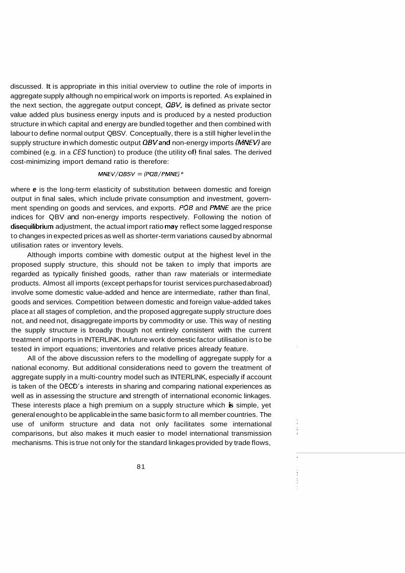
Estimation results for the investment demand equations are presented in Table 5, and estimated and actual growth rates of business gross fixed investment are displayed in Chart 5. Unfortunately, in no case was the coefficient estimate for a3 correctly signed and the integral adjustment term was therefore omitted. Equation ( 15) represents an error correction specification22 where the adjustment is one of investment towards desired capital stock. Because this stock is related to expected output, the model implies a constant capital-expected output ratio in the long run under general assumptions. The IFUeffect was present in free estimation in all countries except France and Canada, although statistically significant only for Germany and Italy. The profitability hypothesis receives support in four cases, and the effect was imposed in the United Kingdom and Canadian equations; for the United States a4 was competitive with a5, and the latter was judged more important. The tracking performance of the equations for Canada and the United Kingdom is the least satisfactory, probably owing to the fact that in those two countries energy investment has played an important role: the investment series have not yet been properly adjusted to remove energy investment from total investment, as required by the logic of the supply block structure.
The labour demand function can equally be specified as an error correction equation:
LN(ETB/ETB(- I)) = a. + a1 In(EBSTAR/EBSTAR(- 1 ) ) + a2 In(EBSTAR(- l)/ETB(- 1 ) ) + a3 In(CQBl + a4 In(lFU) + U
(16)
EBSTAR, or desired employment, is defined as the number of workers required to produce the expected future profitable output QBSTAR with the desired capital stock KBSTAR and the corresponding energy input. It is calculated by inverting the aggregate production function:
EBSTAR = ( ( (QBSTAR~~ - 1 m - (XOGAMA.((QBSTAR.(XOGAMA + (XOBETA 5 . (XOGAMA. ((WSSE/ELEFF)/CKE)I1- c) ) cl(’- 5’)) ( c-1)/ r)))/XOBETA) r / ( T-l))/ELEFF
103

Table 6. Business employment equations
In(ETB/ETB(- 7)) = a0 + al In(EBSTAR/EBSTAR(- 1)) + a2 In(EBSTAR(- l)/ETB(- 1 ) ) + a3 In(CQl3) + a4 ln(lFU) + U
Estimated coefficients (t-statistics)
United States -0.01 0.60 0.20 - 0.09 66S1-8282 (-2.8) (7.7) (3.5) (2.6)
Japan - 0.28 0.02 - - 6682-8282 (5.2) (4.2)
Germany -0.01 (-4.4)
France -0.01 (-3.6)
United Kingdom -0.02 (-4.0)
Italy -0.1 (7.0)
Canada 0.00 (0.5)
0.23 (4.3)
0.29 (5.2)
0.23 (3.9)
0.29 (2.8)
0.40 (5.0)
0.13 -0.15 (3.6) (-6.5)
0.14 - (3.9)
0.23 -0.04 (3.2) (-3.4)
0.10 -
(i)
0.01 - (0.1 1
0.1 5 6681-8282 (5.3)
0.06 6681-8282 (2.1)
0.06 67S1-8282 (1.1)
0.10 6781-8282 (i)
0.1 5 66S1-8282 (1.4)
(i) Coefficient imposed.
Regression statistics
R2 DW SEE
0.77 1.4 0.0055
0.38 2.1 0.0049
0.89 1.6 0.0031
0.54 1.8 0.0033
0.80 2.0 0.0045
0.25 1.5 0.0089
0.74 1.2 0.0080
Estimation results for the employment equations are presented in Table 6, and estimated and actual employment growth rates are displayed in Chart 6. The integral adjustment parameter had to be imposed for Italy, and its estimate is disconcertingly small for Canada. Profitability effects are identified only for Germany and the United Kingdom. IFU effects are found for all countries except Japan and Italy; in the latter a non-zero parameter was imposed for the sake of overall model properties. The apparent weak performance of the equation for Italy is due mainly to the failure to capture some of the large semi-annual employment growth fluctuations, especially during the first half of the sixties. These large periodic fluctuations look peculiar, however; they may be due t o deficient seasonal adjustment procedures.
104

40 1
28 18 08 6L 8 1 LL 9L SL t L EL ZL I L OL 69 89 L9 99
10 0- 10 0-
0 0
10 0 10 0
E0 0- E0 0-
zo 0- 20 0-
10 0- 10 0-
10 0- 10 0-
0 0
10 0 20 0
0 0
t o 0 t o 0
10 0 10 0
20 0- zoo- 100- 10 0-
10 0- 0
10 0- 0
0 0
10 0 L O O L O O 10 0
20 0 20 0 20 0 10 0
1 8 18 08 6L 8L LL 9L SL t L EL 2 1 1L OL 69 89 L9 99 €0.0-
28 18 08 6L 8L LL 9L 51 VL EL ZL LL OL 6 9 89 1 9 EO'O-
20'0- zo.0- ZO'O- - ZO'O- -
- 10'0-
10'0-
0
10'0

The means and variances of the dependent variables for the factor demand equations for each country are shown in Table 7. A striking feature of this table is the low variance of employment change in Japan. This suggests that in Japan the labour market may be flexible enough for employment to be determined by slowly moving demographic factors, with variations in output and profitability leading to redeployment and changes in the utilisation rate rather than to changes in employment.
Country Sample period
Table 7. Moments of changes in factor input variables
Mean Standard Mean Standard Mean Standard deviation deviation deviation
United States S2.60-S2.82 Japan S2.66-S2.82 Germany S2.60-S2.82 France S2.63-S2.82 United Kingdom S2.60-S2.82 Italy S2.60-S2.82 Canada S2.60-S2.82
0.0084 0.0099 0.0050 0.0057
-0.0025 0.0082 0.0008 0.0042 -0.0032 0.0089 -0.001 1 0.01 10
0.01 15 0.01 35
0.01 95 0.0410 0.0465 0.0870 0.01 48 0.0455 0.0214 0.0331 0.01 65 0.0388 0.01 30 0.0543 0.0229 0.0426
0.01 01 0.0302 0.0205 0.0500 0.01 11 0.0308 0.01 32 0.0351
0.01 65 0.0379 0.0541 0.0428
-0.001 1 0.0291
The basic structure of the business energy demand (€/VBV)equation is different from the one chosen for the employment and investment demand equations because energy inputs can be adjusted to optimal levels without delay: the vintage energy requirement (EBSV) is given by equation (3) in section 1II.C above. This is the optimal energy input subject to the existing and partially retrofitted vintage capital stock. Although there are no adjustment lags in the demand for energy, actual energy demand (ENBV) may deviate from "normal" energy requirements because of abnormal factor utilisation rates. This leads to the following energy demand equation:
/n(ENBV/ENBV(- 7)) = a0 + a1 in(EBSV/EBSV(- 1 ) ) + a2 In(lFU/IFU(- 1 ) ) + U (17)
In all countries outside North America a weak negative constant term implies some autonomous restraint on energy demand growth, probably reflecting energy-saving technical progress or the effects of administrative (non-price) measures to save energy. Estimation results for the energy demand equations are
106

CHART 7
BUSINESS ENERGY DEMAND (GROWTH RATE)
-Actual ....... Predicted United Kingdom
0.08 r Germany 0.08 0.15
0.04 0.04 O . l o
0.05 0 0
0 -0.04 -0.04
-0.05 -0.08 -0.08
-0.10 61 63 65 67 69 71 73 75 77 79 81
1 France
I-
0.08 0.08
0.04 0.04
0 0
-0.04 -0.04
-0.08 -0.08 64 66 68 70 72 74 76 78 80 82
107
Canada , 0.15
--0.10 61 63 65 67 69 71 73 75 17 79 81

Table 8. Business energy demand equations
In(ENBV/ENBV(- 1)) =a0 + a1 In(EBSV/EBSV(- 1 ) ) +a2 In(lFU/IFU(- 1 ) ) +U
Regression statistics Estimated coefficients
a0 a1 a7 R2 SEE DW RHO
Estimation (t-statistics) period
Country
United States 196082 198282
Japan 196582 198282
Germany 1960S2 198282
France 196382 198282
United Kingdom 196381 198282
Italy 196082 198282
Canada 196082 198282
0.0009 (0.1)
-0.002 5 (-0.3)
-0.006 8 (-1.2)
-0.003 1 (-0.4)
-0.01 45 (-1.9)
(-1.3)
0.0083 (1 .O)
0.0072
0.19 (0.5)
0.49 (1.1)
0.52 (2.6)
0.1 7 (0.7)
0.32 (1.4)
0.15 (1.1)
0 (0.0)
0.35 0.023 1.7 0.50 (4.6)
0.16 0.034 1.5 0.34 (2.2)
0.31 0.022 1.6 0.43 (3.3)
0.27 0.024 1.6 0.49 (3.4)
0.32 0.025 1.6 0.47 (3.3)
0.32 0.019 1.7 0.51 (4.0)
0.23 0.029 1.3 0.46 (3.6)
(i) Coefficient imposed.
presented in Table 8, and graphs of estimated and actual growth rates of energy demand are displayed Chart 7. The coefficient (a , ) was constrained to unity for all countries, thereby forcing the instantaneous response of actual energy demand to changes in vintage energy requirements to be proportional.
VI. LINKING THE SUPPLY BLOCK TO PRICE DETERMINATION
The production structure outlined in the preceding section has been linked to the price formation process in INTERLINK to complete the supply side of the model. The price of gross business output corresponding to the level of aggregation in the supply structure (gross value added plus intermediate energy inputs) is the aggregate output deflator PQB. Actual value-added prices (including supra-normal
108

mark-ups, whether positive or negative) will depend inter alia on the prices of foreign competitors, approximated by the country's unit import prices. The latter influences the cost mark-up that producers are able to charge. Of course, import prices are also present in the final domestic expenditure deflator equations. The disaggregated import price series currently in INTERLINK have therefore been reweighted according to the industrial structure of the individual importing country, because the commodity structure of imports may differ substantially from that of domestic output (for example, Japan). The resulting series, PMQ, is used in the determination of PQB.
A cost index CKEL is computed from the dual to the aggregate production function, i.e.
CKEL = (XOBETA. (WSSE/ELEFF)('-T) + XOGAMA. C K E ( 7 - r ) ) ( 1 / ( 7 - r ) ) ( 1 8 )
where CKEis the cost index of the capital-energy bundle, computed from the dual to the inner (marginal) CES function which aggregates capital and energy into the increment to the input bundle KEBSV:
CKE = (XIBETAS. UCc(7-ss, + XlGA MAs. PEfVB(l-s))(l/f r-s)) (19)
An additional domestic cost measure which does not assume that prices are set based on full adjustment of factor inputs to changes in relative factor prices is also included. It is defined as:
COST = (WSSE. ETB+UCC.(KBV+ KBV(-7))/2+ PENB. ENBV)/QBSV (20)
where WSSE is private sector compensation per employee. In addition, cyclical effects from inventory disequilibrium as well as from
changing rates of factor utilisation were assumed to influence the price formation process. However, proxying the former by the ratio of actual inventories to the product of normal output and the mean of the historical average stock-output ratio led to little success. Accordingly, the effects of aggregate demand on prices are limited to the direct IFU channel. Long-run homogeneity has been imposed ex ante with respect to costs and import prices and, where necessary, dummy variables and time trends were included in the estimation but not in the model code. Rather free estimation of dynamics was allowed. Accordingly, the general form of the equation was:
b C
i = l j = O In(PQB,) = a0 + Z al;ln(PQBt-j) + Z azjln(CKELt.,)
109

Table 9. Business output deflator equation
d e f
k=O I= 0 m=O a3kln(COSTt-k) + 2 a411n(PMQt-J f 2 a5,,, InllFU,,,,) -+ Ut
Canadab United United Statesa Japanb GermanyC Franced Italy
a0
a l l
a 12
a20
a2 I
a22
a23
a24
a30
a3 1
a32
a33
a34
a40
a4 1
a42
a43
0.0069 (4.64)
0.7960 (22.89)
0.51 08 (i)
(4.08) -0.3398
0.0330 (7.82)
0.9550 (i)
0.6232 (9.97)
-0.3971 (3.25)
(2.74)
0.1921 (1.75)
-0.0844 (1.45)
-0.31 13
0.0225 (1.45)
0.0236 (7.45)
1.021 6 0.5446 (8.98) (5.75)
-0.301 9 0.3089 (3.84) (3.10)
0.2230 ( i )
0.7367 (1.82)
(9.46)
(3.04)
-0.3 7 7 3
-1.0832
0.0573 (8.92)
0.5053 ( i )
(1.82) -0.7367
1.0832 (3.04)
1.1999
-0.3094
(16.18)
(4.58)
0.3297 (i)
-0.2484 (4.80)
0.7691 (12.17)
0.7396 (6.59)
(6.59) -0.7396
-0.2692 (3.45)
0.3580 (3.69)
0.1421 ( i )
0.0283 (2.03)
1.0642 (9.1 6)
(2.89) -0.2903
-0.4201 (4.70)
0.1443 (3.40)
0.4201 (4.70)
0.081 8 (i)
110

Table 9 (cont'd).
Italy Canadab United Japanb GermanyC Franced Kincldome United Statesa
a44
a50
a5 7
0.01 84 (1.13)
0.02 0.1320 0.0972 0.14 0.1293 0.1367 (i) (2.72) (1.96) (i) (1.26) (3.05)
a52 0.1 109 (3.95)
RSQ 0.9999 0.9995 0.9998 0.9999 0.9999 0.9997 0.9998 SEE 0.0029 0.0077 0.0045 0.0036 0.0078 0.01 18 0.0069 DW/h
Sample 63S1-8282 6781-8282 6482-8282 66S1-8282 65S1-82Sl 6382-82S2 63S1-8282 - (i) Coefficient imposed. a)
b) cl d) e) f l
Also includes a dummy variable equal to unity for 66S1-69S2 and 76S1-78S1 as well as a high-order term in time. Also includes a dummy variable equal t o unity for 74S2. Also includes a dummy variable equal t o unity for 7052 and minus unity for 71 S1. Also includes a dummy variable equal t o unity for 74S1 and minus unity for 75S1. Also includes dummy variables equal to unity for I 1 Sl, 73S1, 73S2. 7982 and 80S1. Also includes dummy variables equal to unity for 75S2 and for 76S1-78S1.
In practice, b = 2, c = d = e = 4, f = 2. All insignificant parameters were eliminated. Estimation results are given in Table 9, long-run elasticities in Table 10 and estimated and actual growth rates of PO6 in Chart 8.
In general, the fits are fairly good. The averse elasticity of prices with respect to domestic costs is 0.73 in the long run, while the remaining 0.27 emanates from import prices. Import price elasticities vary from 0.13 for France and 0.16 for the United States to 0.50 in Japan. The Japanese result is somewhat strange, but it should be noted that the mean lag is in excess of 2 1 semesters and that the short- and medium-term import price feed-through is relatively small. The COST variable tends to dominate in Japan, France, Italy and Canada, while CKEL dominates for the
111

0.03
0.02
0.01
0
0.20
0.15
0.10
0.05
0
-0.05
0.05
0.04
0.03
0.02
0.01
0
-0.01
CHART 8
BUSINESS OUTPUT DEFLATOR (GROWTH RATE)
-Actual
- United States
-
63 65 67 69 71 73 75 77 79 81
I...-- Predicted
0.06 0.16
0.05
0.04
0.03 0.08
0.02
0.01
0 0
United Kingdom r 1
0.12
0.04
0.16
0.12
0.08
0.04
0
1 0.16 Japan Italy r 1 o.20 0.16 r -
0.12 A 0.15 0.12 -
0.08 0.08
- 0.05 0.04 0.04
I , 0
I I I I I I I I I I I I I ~ ~ ~ ~ ~ ~ ~ ~ ~ ~ ~ ~ J ~ ~ l 0 0 --0.05
68 69 70 71 72 13 74 75176 77 78 79 80 81 82 64 66 68 70 72 74 76 78 80 82
-l Germany -, 0.05 Canada r
- 0.08 0.08 0.04
0.03 0.06 0.06
0.02
0.01 0.04 0.04
-
0.02 0.02 - 0
I l l I’ I I I I I I I I I I I I I I l l I I , I I -0.01 0 0
65 67 69 71 73 75 77 79 a1 63 65 67 69 71 73 75 71 79 81
0.04
France
A
- - 0.02 -
66 67 68 69 70 71 72 73 74 75 76 77 78 79 80 81 82
112

Table 10. Long-run business output deflator elasticities
United States CKEL 0.84 COST 0.00 PMQ 0.16 IFU 0.54
Japan CKEL COST PMQ IFU
Germany CKEL COST PMQ IFU
France CKEL COST PMQ
0.00 0.50 0.50 0.44 (i)
0.80 0.00 0.20 0.47
-4’94 0.87 5.81 0.13
United Kingdom CKEL 0.74 COST 0.00 PMQ 0.26 IFU 1 .28 (i)
Italy CKEL COST PMQ IFU
Canada CKEL COST PMQ IFU
Unweighted mean CKEL/COST PMQ IFU
-1.17 1.91 0.26 0.56
-1.22 1.86 0.36 0.60
0.73 0.27 0.55a
0.74
0.64
IFU 0.66 (i) Coefficient imposed. a) Excluding the United Kingdom.
other three countries. Significant FU effects are in evidence for the United States, Germany, France and Canada. Parameter impositions had to be effected for Japan and the United Kingdom; a large value was chosen for the latter in order for the model to generate reasonable overall simulation properties: not much inflation is generated by the United Kingdom wage equations (Coe, 1985).
The business output price PQB and the business value added deflator (at factor cost, PGDPB) are connected by the following identity:
PGDPB = (PQB-PENB.ENBV/QBV)/(GDPBV/QBV) (22)
The GDPdeflator can in turn be computed from the business value added deflator by identity:
PGDP = (PGDPB.GDPBV+ TIND-TSUBf CGW)/GDPV (23)
where CGW is nominal government expenditure on wages and salaries. Individual demand component deflators were computed as weighted averages of the business
113

value-added deflator, import price deflators and net indirect taxes, using aggrega- tion weights approximately corresponding to the appropriate input-output coeff i- cients. The weights were imposed, and no deflator-specific IFU terms have been included, but work is underway to remedy these deficiencies using mixed-regression techniques.
VII. ENDQGENISING LABOUR SUPPLY
In order to capture additional supply-side effects in the labour market, the new labour demand equations discussed above and the existing wage equations in INTERLINK have been supplemented by labour force participation equations. (Previously, the labour force was treated as if it were exogenous.) This completes the modelling of the labour market, endogenising unemployment and hence determining wages more satisfactorily. Equations were estimated for males and females separately, given the frequent contrary developments of their participation rates.
The initial specification was ad hoc. One group of variables proxies socialldemographic factors which cannot be adequately endogenised in a macro- economic model. Nevertheless, such variables were included at the estimation stage to preclude biased estimates of coefficients on "economic" variables. The age structure of the population is a potentially important influence on participation rates. This was tested in two ways: first by a variable AGE, defined as the logarithm of the ratio of actual and age-constant participation rates with an indeterminate sign e~pecta t ion~~; secondly the shares of those under the age of 25 (YOUTH) and those over 55 (OLD) in the working-age population were included as explanatory variables. Initially AGE, YOUTH and OLD were included jointly in the equation. Participation rates are also likely to be affected by rates of family formation and childbearing. The ratio of the number of children under the age of 5 to women in the 20 to 34 age bracket (DEP) was accordingly included in both equations with a weak positive sign expectation for males and a negative expectation for females. Continuing education is an alternative to labour force participation, so that the larger the number of people in the20 t o 2 4 age bracket enrolled in post-secondary institutions (ENR), the lower should be their probability of labour force participation. Finally, employment opportunities for women differ across sectors, with services displaying the highest female representation. It is possible that women will enter the labour force in response to the long-term structural shift in OECD countries towards the production of services, with resultant enhanced employment opportunities. The
114
share of services employment (SERF) is included, with a positive sign expectation in the female equation and an uncertain sign expectation in the males equation.
A second group of explanatory variables comprises the economic factors which are endogenous in INTERLINK. First, there are possible cyclical effects: potential labour force participants probably base their entry decision on the expected probability of success from job search - high unemployment yields the well known "discouraged worker effect". However, the decision of some secondary workers to enter and exit may be based on the employment status of their spouses. Unemployed workers can cause other household members to seek work - the "added worker effect". The net cyclical effect is therefore to some extent unclear, although it seems likely that the discouraged worker effect will dominate, so that the participation rate will be procyclical. In general, the specification includes the aggregate unemployment rate (UNR) with a (qualified) negative sign expectation, especially for males, as well as the factor utilisation rate, with a positive sign expectation. In the case of Japan, however, aggregate emp!oyment itself was directly inserted into the equation, in response to the well known low variance of the historical series for UNR in Japan.
The real wage is expected to have a positive effect on participation rates, by increasing the (opportunity) cost of leisure and/or other unremunerative activity. Given that participation decisions are made within a family unit there may also be a negative income effect on participation rates from higher real wages, when a family member leaves the labour force because of increased earnings by another member. The earnings concept used is wages per employee net of household direct taxes (TYH) and social security contributions (TRSSH), deflated by the consumption deflator, i.e. RW = ((WSSS-TYH-TRSSH)/EE)/PCP.
Non-wage incomes can be expected to be negatively related to participation decisions because they have no associated substitution effects. The aggregate non-wage income is scaled by working-age population, and the resulting series is deflated using the private consumption deflator. Where data are available interest on consumer debt (INTDBT) is removed, but government transfers are not included in the resulting term (NWY). Government transfers (TRRH) are treated separately, because in addition to the negative income effects, there are also possible negative incentive effects. Here too, the scale variable used is working-age population, and deflation is by the private consumption deflator, yielding the proxy GT.
A double-log specification is used. While the dependent variable is limited to a range between zero and unity, experience shows that usually only trivial differences in parameter estimates are found when probidlogit procedures are used, and accordingly "ordinary" estimation techniques were applied. However, because the equations for the two sexes will have cross-correlated error structures, both OLS
115

and Zellner-eff icient "seemingly unrelated regression estimators" were used. The simultaneity problem has, however, been neglected to this point, as has the possibility of cross-country correlation of error structures. The preliminary specification is therefore:
LFPRIjt = MO,, + M1l,.AGE,t + M2+. YOUTHljt + M3lpOLDut + M4yDEP)i
+ M5yENRyt + MsrSERF,, + MTyUNRjt + MsyIFUyt
+ M9yRW.t M70yNwYjt + Mll+.GT,t + M72yLFpRyt-1 + eyt
where; = females, males j = 1, ..., 7 (the Big Seven) t = time, by semesters e is a conventionally-defined error term, with r(evt, emit) # 0 assumed
M2, M3, M4ft M5, (M7), Mio, Mii G 0 (parentheses indicates caution).
The estimation strategy was to begin with the full specification but to exclude variables with insignificant and/or perverse and marginally significant coefficients. However, where necessary to whiten residuals, various polynomial functions of time were included, as were longer lags on the dependent variables and Cochrane-Orcutt corrections for first-order serial correlation of the error terms.
A summary of estimation results is given in Table 1 1. The Canadian equation is for the aggregate labour force because of convergence problems with the sex-disaggregated equations. The average standard error of estimates is one-third of 1 per cent.
Many of the "social" variables are statistically significant. The age variable has a significant coefficient in about half the equations, with all but one sign being positive. In general, it appears to be more important in the equations for women than for men, which is reasonable given the more substantial changes that have occurred in women's social and economic roles over the estimation period. The youth proportion has the expected negative elasticity in only five of thirteen cases, with three estimates perversely positive. The share of the elderly similarly takes a negative coefficient in five cases and a positive one in two, although the Japanese males effect is more than wiped out by the effect from Japanese women. The effect is by,far the most substantial in the United States. The number of infants per woman of child-bearing age takes the expected negative sign in only three of the six females equations and has a perverse positive parameter estimate for French women. There
116

Table 1 1. Participation rate equations
United States
Females Males
AGE YOUTH OLD DEP ENR SERF UNR IFU RW NWY
LDVl LDV2 RHO Weighted SEE
2 GT A
4
-0.05 -0.94 -0.59 -0.05
-0.03 +0.76
+0.07 +0.06 -0.06 -0.05
+0.56 +0.40 -0.21
-0.34 0.0036
Japan
Females Malesb
t0.06 +9.002 -0.41 -0.20 +0.01 -0.29
t0.69 t 1.37a +0.99a
-0.05 -0.08
-0.31'
0.001 9
Germany
FemalesC Males
-0.02 +0.01 -0.10 -0.06 -0.24
t0.49 -0.01 -0.004
t0.06 -0.03
+0.82
-0.33 0.002 1
United Kingdom
Femalesd Males
-0.13
t 1.48
t0.14 t0.03
-0.004 -0.001
-0.03
+0.75
0.0036
France
Femaless Males
t0.06 +0.01 t0.32 +0.12 t0.25 t0.26
-0.25 -0.05 t0.12 t0.14
-0.006
t0.33 +0.4If
0.001 7
Italy
Femaless Males
t0.07 +0.44
+0.23 -0.1 7
t2.64 t0.04
-0.09'
-0.25 +0.20
0.0067
Canada
Totalh
-0.49
t0.60
t0.23 -0.03
-0.07 -0.04
1.0040
al For Japan the regressor is actually total employment scaled by the working age population in the females equation; in the males equation it is both current and one-semester lagged scaled employment with elasticity estimates of 1.22 and -0.23. respectively. (See i below.)
6) The equation also includes the female participation rate with an elasticity of -0.47. cl The equation includes a second-order polynomial on TIME prior to 1975 as well as an inverse on TIM€ thereafter. dl The equation includes an inverse on TIME. el The equation includes the male participation rate with an elasticity of -0.88 and a second-order polynomial and an inverse on TIME. f l The equation actually includes four lags on the dependent variable with elasticity estimates as follows: 1.1 9, -1.31, 0.76, -0.24. gl The equation actually includes a second-order polynomial and an inverse on TIME. hl The equation actually includes a second-order polynomial on TIME. il After estimation it was decided to (1 ) remove the perverse RWcoefficient in the Italian LFM equation; (2) remove the negative second-order lagged dependent variable in
the Japanese LFM equation: and (3) remove the lagged employment term in the Japanese LFM equation. No re-estimation was undertaken.

are also positive parameters for males in Italy and Canada. The enrolment rate variable was available only for the United States for this project and apparently influences only males' participation decisions. Last among the "social" regressors is the service industry variable, which has the expected positive effect in all female cases except France, where it comes indirectly from the male cross-effect. It is strongest for Italy and the United Kingdom and weakest for France and Canada.
Among the "economic" variables, the cyclical proxies are apparently significant determinants of the participation rate in all cases except for American, French and Italian men. In five of the six cases where a sex comparison is possible the female rate is more procyclical than the male rate; only in Italy does the added-worker effect dominate the discouraged worker effect for women. The unemployment rate seems to be a better proxy for the effect of the cycle in the labour market than the factor utilisation rate coming from the supply block. However, for British and French women the two are both individually significant. For Japan the use of the employment rate gave apparently reasonable estimation results: the long-run elasticity of the labour force with respect to total employment is 1.37 for women and 0.45 for men, with a weighted average of about 0.8. However, the Japanese model proved too inflation-prone in simulation, and it was decided to remove the lagged employment term and the lagged dependent variable from the LFMequation, thereby raising the male elasticity to 0.58 and the weighted average to about 0.89.
The real wage turns out to be the most difficult economic variable to interpret. Wages disaggregated by sex are not available, so the same aggregate average earnings rate was used in both equations. It has a statistically significant influence in only about half the equations estimated, and of these almost half are in a negative direction. A negative effect for women could be justified by the second-earner nature of many women in the labour force: when their spouses' incomes increase, the income effect may indeed dominate the substitution effect in the determination of their demand for leisure, and they may not only reduce their desired hours of work but may indeed drop out of the labour force altogether. However, the German and Italian results manifest negative coefficient estimates in the males equations, and this is harder to accept, suggesting as it does that the aggregate labour supply curve is backward-bending. Yet, the Canadian model shows a negative effect in the aggregate. So did the Italian model, but this was eventually set to zero. Further work in this area will aim to overcome this deficiency.
Non-wage income other than government transfers leads to an observable negative income effect on the demand for leisure, but only in a limited number of cases. There is no observable effect at all for Germany and Italy. Furthermore, an additional disincentive effect from government transfer income can be empirically
118

detected only in the case of Japanese females. For British and French men as well as Canadians in general even the pure income effect is not in evidence. Adjustment of actual to equilibrium participation rates is seen to be quite rapid, except in the cases of German and British men, where the mean lags reach 2.3 and 1.5 years, respectively.
The procedure used to insert the equations into INTERLINK, given the desire to avoid inclusion of additional exogenous variables in the model, was to drop the social/demographic variables from the equations, to constrain the other elasticities to equal their values estimated in the first stage, to include a high-order polynomial function on time and its inverse, and to estimate the parameters of that function in a second round of Zellner-efficient e ~ t i m a t i o n ~ ~ . In all cases except the United States, the estimated time polynomial would imply implausible movements in either the male or female participation rates in the near future. Finally, therefore, the equations were implemented with the estimated elasticities of the economic regressors, but with trend effects omitted and the constant terms readjusted to make the average error over the recent past equal to zero. This implies that only the U.S. equations can be used for unconditional forecasting without extensive add-factoring. When used for,counterfactual simulations, the absence of projections of exogenous "social" variables will not affect simulation results.
VIII. CONCLUSIONS
This paper presents production and factor demand equations for the seven largest OECD economies. The linkage of this supply structure to the price formation process and the endogenisation of labour supply are also discussed. In these concluding comments, some of the main features of the estimation results are summarized, indicating areas for possible further development, and suggesting ways in which other parts of the INTERLINK model could be adapted to mesh more effectively with the newly integrated supply model presented in this paper.
For the underlying longer run production function, significant support for the idea of using a vintage bundle of capital and energy in combination with efficiency units of labour was found. Sevcral countries showed quite high long-run elasticities of substitution between capital and energy. Most showed important vintage effects that supported a putty/semi-putty view of technology, whereby energy use is fully flexible before capital is put in place and partially flexible thereafter.
There is evidence for most countries that there has been international convergence in the rate of increase in labour efficiency for the faster growing
119

countries during the 1960s and early 1970s - especially Japan, Germany, France and Italy. This implies a substantial slowing down of the rate of growth of labour
=_efficiency in these countries at the end of the 1970s and in the early 1980s. The -- -size of this estimated catch-up effect may be overstated in the present results,
because the end of the sample period was marked by low utilization rates, and it is difficult to find an adequate means of simultaneously estimating the cyclical and catch-up effects. The hypothesis that technical progress is embodied in new capital equipment was tested, but the results were dominated by the performance of the catch-up specification which accordingly has been integrated into the model as the maintained hypothesis.
Because there is evidence of increasing trends in the wage share that are inconsistent with the assumption of Cobb-Douglas technology for the outer function combining labour with the bundle of capital plus energy, a more general CES form was developed. However, the derived equations for production and factor demands revealed very little power to choose a value for the thereby-freed elasticity of substitution. The evidence suggests that in most countries it could easily be as low as 0.65 or as high as 1 .O, and that the choice has virtually no effects on the fit or the parameter values of the estimated production and factor demand equations. Of course, the effects of wage flexibility or rigidity on the demand for labour, and hence on the unemployment rate, depend importantly on the elasticity of substitution between labour and other factors. Furthermore, changes in the derived demand for labour are an important part of the overall macroeconomic effects of alternative patterns of wage behaviour. Thus, the uncomfortable fact is that important simulation properties of the model are not very well determined on the basis of analysis of historical data.
In terms of future development of the long-term production structure, it would probably be useful to take account of longer-term movements in average hours worked when defining the labour input to the production function. Above (cf. Part 111) the advantages were pointed out of treating cyclical variation in man-hours, and in machine hours, as part of the overall measure of capacity utilisation, QBV/QBSV, because so many other features of utilisation cannot be separately measured. In the present version of the model, any trend changes in hours worked are automatically treated as part of the aggregate index of labour efficiency, thereby reducing the measured growth rate of total factor productivity. As long as the downward trend in hours is a t a constant rate, and likely to remain so, this procedure does not cause problems. However, there is evidence that the downward trend in hours may be slowing down, and in several countries there are discussions of substantial legislative changes in the number of weekly hours. In addition, the levels and trends of average hours differ among countries, and this may disturb international
I
120

con-tparisons of labour efficiency, and affect estimates of the international catch-up hypothesis. For all these reasons, a redefinition of the labour input to include long-term changes in average hours warrants examination.
The short-run production equations provide strong and consistent evidence of systematic and economically explicable variations in the utilisation rate. The use of utilisation rates as the dependent variable for the short-term production decision provide a means of consistently integrating the demands for capital, labour and energy (all combined in the normal output series QBSV) with the factors influencing the intensity of factor use: sales, profitability, and the level of opening inventories. Of the three factors, the sales and profitability effects were empirically the most important.
In all countries, the estimated speed of the production response to an inventory gap is not well determined. However, this does not mean that the inventory level itself will be ill-determined, or that it will wander indefinitely far from its desired value when sales change. This is because the production response to the inventory gap is only one of several possible channels through which inventory equilibrium can be restored. The inventory gap should also influence trade flows, and future work on trade equations in INTERLINK may test this hypothesis. However, initial re- estimation of those equations has not yielded promising results. In addition, any discrepancy between expected sales and desired production that is not matched by desired imports will lead to changes in factor demands, and hence in production capacity and actual output, that will choke off the original pressure to build up or run down inventories.
The estimated equations for investment showed substantial lags in the adjustment of capital to changes in desired levels. To some extent these partial adjustments, and the sometimes substantial unexplained variance in the factor demands, may be due to inevitable difficulties in identifying the desired factor levels. However, the results provide evidence that both capital and labour should properly be regarded as quasi-fixed factors, though with the degree of fixity for capital much exceeding that for labour. This provides further support for treating factor utilization as a short-term adjustment variable used to help mediate between demand conditions and production capacity when the former are uncertain and the latter is costly to adjust.
Recent theoretical work suggests that the investment rate should be directly affected by profitability in conditions of uncertainty and costly adjustment, so that the empirical strength of the profit rate (PROFR) in the investment equations (other than for the United States) is welcome and helps to provide another important element in the macroeconomic adjustment process.
121

The dual cost function to the aggregate production function has been used to link the production structure to the price formation process. As can be expected, the long-term link between factor cost and output prices detected empirically is very strong, as is the link between competitors' prices and domestic price levels in most countries. However, the cyclical impact of variations in factor utilisation rates and inventory/output ratios on output prices is somewhat more difficult to detect empirically.
Overall, the results, while mixed, are moderately encouraging. They support the view that an integrated model of production, factor demands and price formation as outlined in this paper provides a suitable way of building the supply side of an econometric model.
The production, factor demand, price, and labour supply equations reinforce supply considerations in the logic of INTERLINK, thereby making the model a more useful tool for dealing with medium-term issues. In principle, the endogenous determination of production, and hence of inventory changes, should improve the model's short-term performance, although the empirical robustness of this innovation is not yet established. The integration of the short-term and longer-term supply factors should permit the model to make the transition from the short-run conjuncture to the medium-term growth path. If these attractive possibilities prove to be supported by experience with the supply structures for the major seven OECD countries, this might justify extending comparable treatment, with simplifications where required, to the model/ing of other OECD economies.
122

NOTES
1.
2.
3.
4. 5.
6.
7.
8.
9.
10.
1 1 .
12.
Ball (1 973) surveys the structure of the various national models used in project LINK, all of which treat output as essentially demand-determined. Ball notes (1 973, p.90) that inventory demand equations can be thought of as renormalized output equations. However, all of the models he surveys have inventory demand determined by a flexible accelerator, with no role given to supply factors. This contrasts with the RDX2 (Helliwell et al., 197 1 ) procedure, wherein the inventory change equation is recognised as the link between aggregate supply and demand, with the difference between final sales and the output level desired by firms being the key determinant of the change in inventories.
For example, Sargent's (1 976) "new classical" macroeconomic model for the United States determines output in terms of current and lagged employment plus a time trend.
In METRIC (1 981 1 aggregate supply in most periods is determined by expected final sales and some fraction of the gap between actual and desired inventories. However, whenever the margin of unused capacity drops below 16.5 per cent, there is a reduction in the fraction of expected final sales that is supplied by domestic output and imports; the gap is therefore made up from inventory reductions. Because the resulting inventory discrepancy does not directly influence price formation, the modelling of the supply-constrained regime is not complete.
This work is described in Artus (1 983). For example, Lundberg ( 1 937) and Metzler (1 941), as characterized by Allen (1 968).
Employment is a quasi-fixed factor because of costs of hiring and firing and of assessing the quality of heterogeneous workers. Energy is quasi-fixed because it is complementary with fixed capital, with only limited possibilities for adapting the latter after installation.
See also Annex A for a complete annotated list of equations relating to the production structure. This Annex also describes how the various parameters characterising the production structure were estimated.
It is for these reasons, as well as overall considerations of model management, international comparability and resource implications, that a suggestion of Klein (1 978) has not been followed, namely that the most appropriate way of modelling the interplay of macroeco- nomic supply and demand is to combine a Keynesian set of demand-side equations with a disaggregated supply side based on a Leontief inter-industry model.
This statement refers to general government only; investment and employment by public enterprises are part of the "business sector", in line with standard SNA definitions.
For example, intermediate energy expenditures in the seven largest OECD economies in 1982 amounted on average to 10 per cent of total labour costs.
In principle, the output measure should exclude value added in the energy sector, but as in the case of capital and labour inputs, this adjustment has not yet been implemented.
See the following section and Annex A for a detailed exposition of the algebraic transformations involved.
123
13.
14.
15.
16.
17.
18.
c -
19.
20.
21
22.
23.
24.
As in the previous supply block, this assumes that scrapping proportionally affects all vintages of capital, rather than being concentrated on marginal vintages.
PIM is defined as follows:
PIM = (QBV-r - XOGAMA.KEBSV-r)-l/r/ ETB where r = (1 - Z} /Z
0.99 was used as a Starting point because of problems with using unity in the definition of PIM. PIM turned out to be rather insensitive to changes in Z , and the procedure converged rapidly.
The slowdown effect in the United States evident from the significant coefficient in Table 2 (last column) depends bntirely on the rapid cyclical recovery of productivity from the 1961 recession : if the first three years are excluded from the relevant regression, the slow-down coefficient remains statistically insignificant.
This holds a forfiorifor output per employed person which - apart from labour efficiency - will be influenced by capital and energy input per worker.
The precise definition of the inverted profitability variable is:
COB = (WSSEXTB + ENBV.PENB + KBV.P/B/lOO. (RSCRB + RES + DFR.IRL))/(PQB.QBV)
where DFR is the average debt financing ratio, and RES is computed as a residual, so that on average all factor payments exhaust total output over the sample period and the sample mean of COB equals 1 .O.
Work is currently underway to respecify the output supply equation in a way which would (1 ) add ENBV, subtract only MGSV and possibly add "normal" inventory growth to the numerator of the demand term, and (2) allow for dynamics in the supply response by including one-semester lags on each of the independent variables.
The precise formula is:
PROFR = PQB . Q B V . (7 - COBN(PlB.(KBV + KBVf- 1))/2)
TO the (substantial) extent that the stock market uses current profits as a proxy for the discounted present value of expected future profits, the variable COB is closely related to the inverse of Tobin's q (1 969). Several recent papers (e.g. Yoshikawa (1 9801, Hayashi (1 982) and Abel(1984)) have confirmed that q, or equivalently COB and PROFR, ought to influence the rate of investment when there are adjustment costs. Poterba and Summers (1 983) apply a "q" model to U.K. investment expenditures.
This approach to the modelling of dynamic adjustment paths follows Hendry and Mizon (1 9781, but for simplicity and comparability the number of possible lags was considerably restricted, thereby reducing the complexity of the implied dynamic adjustment path.
The age-constant participation rate is calculated by assuming the age structure of the population is constant at some base year pattern. The (fixed) shares of different age groups in that base year population are then used to weight the participation rates of the age groups in subsequent periods. This yields an aggregate participation rate equal to what it would have been if the population age structure had remained constant.
The standard errors of estimate were all much increased by this procedure, on average by about 8 0 per cent. It would seem that there is therefore substantial information contained in the social/demographic variables.
124
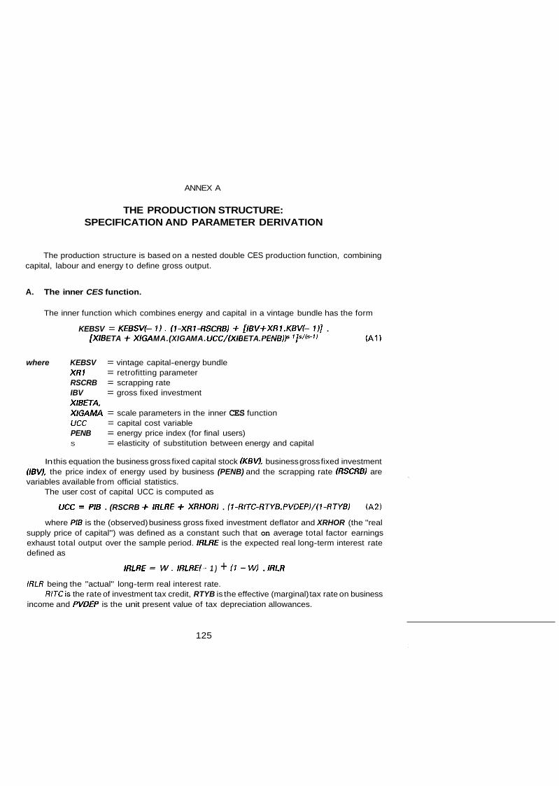
ANNEX A
THE PRODUCTION STRUCTURE: SPECIFICATION AND PARAMETER DERIVATION
The production structure is based on a nested double CES production function, combining capital, labour and energy to define gross output.
A. The inner CES function.
The inner function which combines energy and capital in a vintage bundle has the form
KEBSV = KEBSVI- 1 ) . (7-XR1-RSCRB) f [IBV+XRl.KBV(- l ) ] . [XIS ETA + XlGA MA. (XIGA MA. UCC/(XlB ETA. PENB)P- l]s/(s- (A1 1
where KEBSV = vintage capital-energy bundle XR1 = retrofitting parameter RSCRB = scrapping rate IBV = gross fixed investment XIBETA, XIGAMA = scale parameters in the inner CES function UCC = capital cost variable PENB = energy price index (for final users) S = elasticity of substitution between energy and capital
In this equation the business gross fixed capital stock IKBV), business gross fixed investment (IBV), the price index of energy used by business (PENB) and the scrapping rate (RSCRB) are variables available from official statistics.
The user cost of capital UCC is computed as
UCC = PIS . (RSCRB + lRLRE + XRHOR) . (l-RITC-RTYB.PVDEP)/(7-RTYBI (A2)
where PIS is the (observed) business gross fixed investment deflator and XRHOR (the "real supply price of capital") was defined as a constant such that on average total factor earnings exhaust total output over the sample period. IRLRE is the expected real long-term interest rate defined as
IRLRE = W . IRLREI- 1 ) + (7 - W) . IRLR
IRLR being the "actual" long-term real interest rate.
income and PVOEP is the unit present value of tax depreciation allowances. RlTCis the rate of investment tax credit, RTYB is the effective (marginal) tax rate on business
125

Assuming that the capital-energy ratio (EK) is optimal (subject to prevailing relative prices
XIGAMA/XIBETA = (MEAN(EK)/MEAN [(UCC/PENBP]) (A31
which allows direct computation of X/GAMA/X/t?ETA from observed variables for any given value of s, the elasticity of substitution between capital and energy. Normalising KEBSV such that MEANfKEBSV) = MEAN(KBV) allows XIBETA to be computed as
XIBETA = 1 / ( 1 + (XIGAMA/XIBETAP MEAN ((PENB/UCC)l-s) (A41
The elasticity of substitution (s) and the retrofitting parameter (XR1) are determined by
In(ENBV) = alln(EBSV) + U (A51
where U represents the stochastic error term and EBSV is the vintage energy requirement needed to operate the capital stock KBV subject to prevailing relative energy prices (PENB/UCC), defined as
PENB/UCC) on average over the sample period implies that
estimating the energy demand function
EBSV = EBSV(- I ) . (7-XRI-RSCRB) + (IBV + XRl.KBV(- 1 ) ) . ((XIGAMA. UCC)/(XIBETA. PENB)P (A6)
To obtain a starting value, EBSVis set equal to ENBVat the beginning of the sample period, on the assumption that no large and surprising changes in energy prices occurred over the preceding few years.
The parameter pair (s, XR?) which maximised the likelihood function of regression (A51 was chosen as the preferred parameter combination.
This completes the estimation of all the relevant parameters of the inner CES function.
B. The outer GES function
The outer function which bundles labour and the capital-energy aggregate into gross output
(A7)
has the form
QBSV = (XOBETA.(ELEFF.ETB)-' + XOGAMA.KEBSV-r)-l/r
where QBSV = potential output (at normal rates of factor utilisation) XOBETA, XOGAMA = scale factors in the outer CES function ELEFF = labour efficiency index ETB = total employment, business r = substitution parameter in the outer CES function, with
KEBSV 1 / ( 1 + r ) = elasticity of substitution ( Z )
= vintage capital-energy bundle (see above)
Cost-minimising behaviour by producers implies that on average
KEBSV/ETB = ((WSSE/ELEFF)/CKE)l/(l +r) (A81
where WSSE is observed labour cost per man year and CKEis the cost of the capital energy bundle computed from the dual cost function to the inner CES function
CKE = (XIBETAs.UCC7-s + XIGAMAS.PENB1-S)l/('d (A91
126

The parameter Z (= 1 / ( l + r)) was determined from the regression
In(QBV/(ETB.ELEFF)) = a0 + Z . In(WSSE/(PQB.ELEFF)) + U (A101
where PQB is the deflator for gross output (QBSV) at factor cost. Equation (AI 0) requires ELEFF to be known, while in turn the determination of ELEFF requires knowledge of Z (see below). ELEFF and Z were therefore determined by an iterative procedure, starting with an assumed value of S = 0.99 (see footnote 15)
Equation (A7) can be inverted and solved for the labour efficiency bundle
XOBE TA- lr . EL EFF = [(QBSV-r-XOGA MA. KEBSVr)/ETB-r]-l Ir (A I 1)
Assuming that on average the observed input ratios are cost minimising (subject to observed relative factor prices) allows the parameter XOGAMA to be determined as follows:
Where:
MEAN(PKQ) = MEAN((CKE/WSSE) . (QBV/ETI~) -~) MEAN(NKS) = MEAN((ETB/KEBSV)fl+r))
MEAN(PKK) = MEAN(CKE/(WSSE. ETB) . (KEBSV/ETBbr)
A labour efficiency bundle can now be computed as:
XOBETA-l/r . PIM = ((QBV-r-XOGAMA.KEBSV-r)/ETB-r)-l/r) (AI 3)
where PIM is the observed labour efficiency index which includes cyclical variations and is obtained by substituting actual output (QSV) for potential output (QBSV) in the inverted production function (A I 1 ).
This bundle was used as the dependent variable for the various tests of the time invariance of the rate of technical progress and the testing of the embodiment and catch-up hypotheses. Parameter XOBETA can be determined from this bundle by normalising the calculated labour efficiency index such that
ELEFF1971S1 = 7.0
and imposing the constraint that mean (QSSV) equals mean (QBV) over the sample period.
This completes the determination of the parameters for the outer CES function. The values of the structural production function parameters for the inner and outer CES
functions thereby derived are reported in Table 1 in the main text.
127

BIBLIOGRAPHY
Abel, A.B. (1 983), "Optimal Investment Under Uncertainty", American Economic Review 73,
Abel, A.B. (1 984), "The Effects of Uncertainty on Investment and the Expected Long-run Capital
Allen, R.G.D. (1 968), Macroeconomic Theory, (MacMillan, London)
Artus, P. (1983). "Capital, Energy and Labour Substitution: The Supply Block in OECD Medium-term Models". OECD/ESD Working Paper No. 2.
Ball, R.J. (1 973). "The Economic Models of Project LINK", in R.J. Ball, ed., InternationalLinkage o f National Economic Models, (North-Holland, Amsterdam).
Berndt, E.R. and D.0. Wood (1 979), "Engineering and Econometric Interpretations of Energy- Capital Complementarity", American Economic Review 69, pp. 342-354.
Bischoff, C.W. (1 971 ), "The Effect of Alternative Lag Distributions", in G. Fromm, ed., Tax lncentives and Capital Spending, (Brookings Institution, Washington), pp. 61 -1 30.
Coe, D.T. (1 985). "Nominal Wages, the NAIRU and Wage Flexibility", OECD Economic Studies No. 5 (Autumn), pp. 87-1 26.
Hayashi, F. (1 982). "Tobin's Marginal and Average q: A Neoclassical Interpretation", Econome- trica 50, pp. 21 3-224.
Helliwell, J.F. et al. (1 971 1, The StructureofRDX.2, Bank of Canada Staff Research Studies No. 7 (Bank of Canada, Ottawa).
Helliwell, J.F. et al. (1 9851, "Energy and the National Economy: An Overview of the MACE Model", in A. D. Scott, ed., Progress in Natural Resource Economics (Oxford University Press, Oxford).
Helliwell, J.F., P. Sturm and G. Salou (1 985), "international Comparison of the Sources of Productivity Slowdown 1973-1 982", European Econamic Review 28, pp. 157-1 91.
Helliwell, J.F. and A. Chung (1 9851, "Aggregate Output With Operating Rates and Inventories as Buffers Between Variable Final Demand and Quasi-Fixed Factors", National Bureau of Economic Research Working Paper No. 1623, June.
Hendry, D. and G. Mizon (1 978), "Autocorrelation as a simplification and not a nuisance; The transactions demand for money", Economic Journal 88, pp. 549-563.
Klein, L.R. (1978). "The Supply Side", American Economic Review 68, pp. 1-7.
Lundberg, E. (1 937). Studies in the theory of economic expansion, (Stockholm; Reprinted by
METRIC (1 981 1, Une modelisation de I'bconomie francaise, (INSEE, Paris).
Metzler, L.A. (1 941 1, "The nature and stability of inventory cycles", Review o f Economics and
pp. 228-233.
Stock", Journal of Economic Dynamics and Control 7, pp. 39-53.
Augustus Kelley, New York, 1964).
Statistics 23, pp. 1 13-1 29.
128

Nadiri, M.I. and S. Rosen (1 9731, A Disequilibrium Model of Demand for Factors of Production,
Pindyck, R.S. (1 982). "Adjustment Costs, Uncertainty, and the Behavior of the Firm", American
Poterba, J.M. and L.H. Summers (1 9831, "Dividend taxes, corporate investment, and q", Journal
Sargent, T.J. (1 976), "A Classical Macroeconometric Model for the United States", Journal of
Tobin, J. (1 969). "A General Equilibrium Approach to Monetary Theory", Journalof Money Credit
Yoshikawa, H. (1 980). "On the 'q' Theory of Investment", American Economic Review 70,
(National Bureau of Economic Research, New York).
Economic Review 72, pp. 41 5-427.
of Public Economics 22, pp. 135-1 67.
Political Economy 84, pp. 207-237.
and Banking 1 , pp. 1 5-29.
pp. 739-743.
129

GLOSSARY
A B V CG W CKE CKEL COST COB DELEFF EBSTAR EBSV EE ELEFF ELEFUS ENBV ET6 GDPBV GDPV IB V IFU lFUHA T INTDBT IRLR IRLRE KBSTAR KBV KEBSV LF LFF LFM MESV MGSV MNEV PCP PEN6 PGDP PGDPB PI8 PI M PIMADJ PMNE PMQ PQ B PROFR PVDEP QBSTAR
Five years moving average of business sector gross fixed investment (IBV) Government consumption, wages Dual cost, capital-energy (C.E.S. inner function) Dual cost, capital-energy-labour (C.E.S. outer function) Average normal costs Business sector inverse profitability variable Annual growth rate of the trend labour efficiency index Optimal business sector employment Business sector energy requirement Dependent employment, business Trend labour efficiency index US trend labour efficiency index Energy used by business sector Business sector employment Business gross domestic product (at factor cost), volume Gross national/domestic product at market prices, volume Gross fixed investment by the business sector, volume Intensity of factor utilisation, index Predicted value of IFU Interest on consumer debt Long-term real interest rate Expected long-term real interest rate Optimal business sector fixed capital stock, volume Business sector fixed capital stock, volume Vintage capital-plus-energy bundle (C.E S. inner function), volume Labour force - total Labour force - females Labour force - males Imports of energy, volume Imports of goods and services, volume, N A basis Non-energy imports, volume Deflator for private consumption expenditures Deflator for energy used by business sector Deflator for GDP at market prices Deflator for business value added Deflator for business fixed investment Observed labour efficiency index Observed labour efficiency index adjusted for cyclical variations Price of non-energy imports Output weighted import prices Deflator for business gross output Profit rate Discounted present value of depreciation allowances Business sector gross output expectations
130

QBSV Q6.V RSCRB RTYB SALES STOCKV TlND TRSSH TSUB TYH ucc UNR WAGE WSSE wsss
Normal business sector gross output, volume Business sector gross output, volume Business sector scrapping rate of fixed capital Rate of business profit tax Final sales, (final domestic demand plus exports) Total stock, volume Indirect taxes Social security contributions by households Subsidies Direct taxes, households User cost of capital Unemployment rate Wages and salaries excluding social security contributions Compensation per employee, private sector Compensation of employees
131