Supplementary file

Multimodal epidermal devices for hydration monitoringSiddharth Krishnan1,2,*, Yunzhou Shi3,*, R. Chad Webb1, Yinji Ma4, Philippe Bastien5, Kaitlyn E. Crawford1,2, Ao Wang4, Xue Feng6,Megan Manco7, Jonas Kurniawan1, Edward Tir1, Yonggang Huang4, Guive Balooch3, Rafal M. Pielak3 and John A. Rogers8

Microsystems & Nanoengineering (2017) 3, 17014; doi:10.1038/micronano.2017.14; Published online: 5 June 2017

SUPPLEMENTAL NOTE S1: FABRICATION OF SENSORSFabrication procedure for 1× thermal/flow sensor array—bothepidermal and implantablePrepare polymer base layers1. Spin coat with PMMA 495-A2 (poly(methyl methacrylate), spun

at 3000 rpm for 45 s). 495-A4 will also work;2. Anneal at 180 °C for 1 min;3. Spin coat with polyimide (PI, poly(pyromellitic dianhydride-

co-4,4′ -oxydianiline), amic acid solution, Sigma-Aldrich, spun at6000 rpm for 45 s);

4. Anneal at 110 °C for 30 s;5. Anneal at 150 °C for 5 min;6. Anneal at 250 °C under vacuum for 1 h.

Deposit first metallization1. E-beam 10/100 nm Cr/Au Pattern photoresist (PR; Clariant

AZ5214, 3000 rpm, 30 s; Bake 110 °C, 1 min) with 365 nmoptical lithography through iron oxide or Cr Mask (Karl SussMJB3 or MJB4) for 6 s. Cr is for Adhesion, Au is the mainsensor layer;

2. Develop in aqueous base developer (MIF 917);3. Etch Cr with Cr Etchant;4. Etch Au with Au TFA Etchant (KI- KOH solution);5. Remove PR w/ Acetone. Rinse thoroughly with water (2 cycles).

Deposit second metallization1. E-beam 20/500/20/25 nm Ti/Cu/Ti/Au;2. Pattern photoresist (PR; Clariant AZ5214, 3000 rpm, 30 s; Bake

110 °C, 1 min) with 365 nm optical lithography through ironoxide mask (Karl Suss MJB3 or MJB4). Expose for 6 s;

3. Develop in aqueous base developer (MIF 917);4. Etch Au with Au TFA etchant;5. Etch Ti w/ BOE;6. Etch Cu w/ CE-100;7. Etch Ti w/ BOE;8. Remove PR w/ Acetone, IPA.

Apply encapsulation1. Spin coat with polyimide (PI, poly(pyromellitic dianhydride-co-

4,4′ -oxydianiline), amic acid solution, Sigma-Aldrich, spun at6000 rpm for 45 s);

2. Anneal at 110 °C for 30 s;

3. Anneal at 150 °C for 5 min;4. Spin second coat with polyimide (PI, poly(pyromellitic

dianhydride-co-4,4′ -oxydianiline), amic acid solution, Sigma-Aldrich, spun at 3000 rpm for 45 s);

5. Anneal at 110 °C for 30 s;6. Anneal at 150 °C for 5 min;7. Anneal at 250 °C under vacuum for 1 h, in designated PI oven;8. Pattern photoresist (PR; Clariant AZ4620, 3000 rpm, 30 s; Bake

110 °C, 3 min) with 365 nm optical lithography through ironoxide mask (Karl Suss MJB3). Expose for 15 s;

9. Develop in aqueous base developer (AZ 400 K, diluted 3:1);10. Etch in March RIE (200 mTorr, 150 W, 20 sccm O2, ~ 1800 s). If

using nanomaster, use 200 W Polymer recipe for 20 min.

Release, pick up and print onto Silicone Elastomer1. Release in Acetone at 50C for 1–5 min (have to observe closely-

lots of variability in release time);2. Pick up with 3 M Water Soluble PVA Tape;3. E-Beam Deposit 3/30 nm Ti/SiO2 on Device Side of Tape;4. UV-O treat PDMS (either ecoflex or Sylgard 184 10:1) for 5 min;5. Stick Ti/SiO2 side of device onto UV-O treated side of PDMS;6. Dissolve PVA tape in DI Water on hot plate at 100 °C.

SUPPLEMENTAL NOTE S2: TRANSIENT PLANE SOURCE (HOTDISC) ALGORITHMA major limiting factor preventing the complete deployment ofthe transient plane source formulation is the computationallyexpensive nature of the algorithm. In principle, for each individualtime point, the quantity τ is computed, from which D(τ) can beobtained. A standard fitting algorithm requires this quantity to becomputed for each experimental time point, and then iterativelyuntil a local minimum in the error function is obtained. Tosignificantly simplify this procedure, we first computed thequantity D(τ) for the entire range of experimentally observedvalues of τ. This creates a 50 000 point mesh for 0o τo15. Thiscomputed curve appears in Supplementary Figure S5a. This high-resolution mesh implies a one-time computational cost, but theresulting tabulated values can be easily stored in digital memoryafter this initial computation. In implementing the curve-fittingalgorithm, the quantity D(τ) does not need to be computed foreach time point, but can simply be looked up (and rounded up tothe nearest corresponding computed value). On a standard i7

1Department of Materials Science and Engineering, Frederick Seitz Materials Research Laboratory, University of Illinois at Urbana-Champaign, Urbana, IL 61801, USA; 2Departmentof Materials Science and Engineering, Northwestern University, Evanston, IL 60208, USA; 3L’Oreal Tech Incubator, California Research Center, 953 Indiana Street, San Francisco, CA94107, USA; 4Department of Civil and Environmental Engineering, Mechanical Engineering, Materials Science and Engineering, Northwestern University, Evanston, IL 60208, USA;5L’Oréal Research and Innovation, 1 Avenue Eugène Schuller, Aulnay sous Bois 93601, France; 6Department of Engineering Mechanics, Center for Mechanics and Materials,Tsinghua University, Beijing 100084, China; 7L’Oréal Early Clinical, 133 Terminal Avenue, Clark, NJ 07066, USA and 8Departments of Materials Science and Engineering, BiomedicalEngineering, Chemistry, Mechanical Engineering, Electrical Engineering and Computer Science, and Neurological Surgery; Center for Bio-Integrated Electronics; Simpson QuerreyInstitute for Nano/biotechnology; Northwestern University, Evanston, IL 60208, USACorrespondence: Rafal M. Pielak (RPIELAK@rd.us.loreal.com) or John A. Rogers (jrogers@northwestern.edu)*These authors contributed equally to this work

processor running Windows 7 OS, this reduced the computationtime from 4 days to o10 s for each data point. A resultingcurve fit on a representative porcine skin sample is shown inSupplementary Figure S5b.

SUPPLEMENTAL NOTE S3: SIMPLE, ANALYTICAL EFFECTIVEMEDIUM MODELS FOR PREDICTING TRENDS IN THERMALCONDUCTIVITY WITH HYDRATIONThe thermal conductivity of a skin-water composite, kcomposite, canalso be modeled by a simple rule of mixtures, as was done for thedensity and specific heat capacity in equations (9 and 10). Thedependence of kcomposite on water content, x, (0oxo1) can becaptured using two different models that represent upper andlower bounds. The first, a parallel model, appears schematically inSupplementary Figure S6a. Here, the temperatures at theboundaries of the matrix define by y=0 and y= d are fixed atT=0 K and T= 1 K respectively, with the top and bottomboundaries assumed to be adiabatic. An increase in water content,x, corresponds to an increase in the thickness of the water layer inthis matrix. Pure water is more thermally conductive than dry skin(kwater = 0.6 W m −1 K −1 , kdry skin = 0.2 Wm −1 K −1), and the thickerwater layer creates lower resistance to heat flow, and correspondsto a higher value of kcomposite. The thermal conductivity of thissystem, kcomposite, parallel can be written down mathematically as:

kcomposite; parallel ¼ xkwater þ ð1 - xÞkdry skin ðS3:1ÞA different model, assuming a skin-water composite constructedsuch that the skin and water are in series, appears schematicallyin Supplementary Figure S6b. As with the parallel model, thetemperature as at the boundaries defined by y= 0 and y= drepresent are kept fixed at T=0 K and T=1 K respectively, and thetop and bottom boundaries are assumed to be adiabatic. In thissystem, kcomposite, series can be modeled as a function of x using aninverse rule of mixtures and can be written down as:

kcomposite; series ¼x

kwaterþ ð1 - xÞ

kdry skin

- 1

ðS3:2Þ

An exact, theoretical formulation for the 2D case shown in Figure3a can be written down as36

kcomposite; 2D ¼ kdry skinpþ 1ð Þ þ xðp - 1Þpþ 1ð Þ - xðp - 1Þ

� �ðS3:3Þ

where p= kwater/kdry skin. Similarly, for the 3D case, kcomposite can bewritten down as:

kcomposite; 3D ¼ kdry skinpþ 2ð Þ þ 2xðp - 1Þpþ 2ð Þ - xðp - 1Þ ðS3:4Þ

Theoretical curves corresponding to Supplementary Equations(S3.1)–(S3.4), appear in Supplementary Figure S6c. The parallelmodel (black curve) is linear, and defines an upper bound, whilethe series model (red curve) is nonlinear and defines a lowerbound. This linearity in the case of the parallel model andnonlinearity in the case of the series model are consistent withestablished theory on the rule of mixtures. The FEA-computedcurves, as described in section ``RESULTS AND DISCUSSION'', alsoappears in Supplementary Figure S6c (blue and pink points), andclosely match the theoretical curves (blue and pink lines)corresponding to Supplementary Equations (S3.3) and (S3.4).

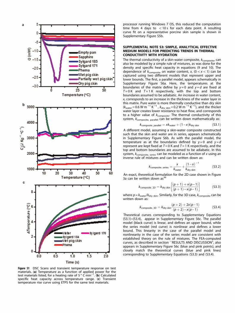
Figure S1 DSC Scans and transient temperature response on testmaterials. (a) Temperature as a function of applied power for thetest materials listed, for a heating rate of 5 ° C min−1. (b) Calculatedspecific heat capacity across temperature range. (c) Transienttemperature rise curve using ETPS for the same test materials.

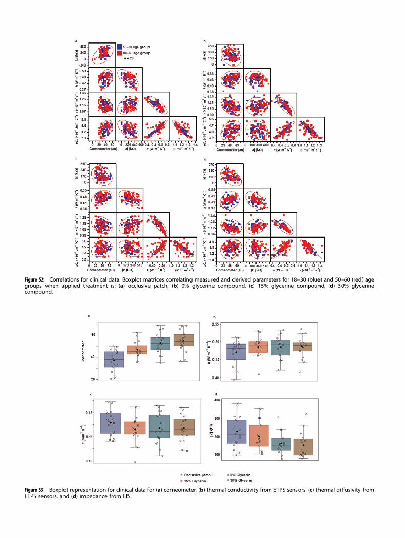
Figure S2 Correlations for clinical data: Boxplot matrices correlating measured and derived parameters for 18–30 (blue) and 50–60 (red) agegroups when applied treatment is: (a) occlusive patch, (b) 0% glycerine compound, (c) 15% glycerine compound, (d) 30% glycerinecompound.

Figure S3 Boxplot representation for clinical data for (a) corneometer, (b) thermal conductivity from ETPS sensors, (c) thermal diffusivity fromETPS sensors, and (d) impedance from EIS.

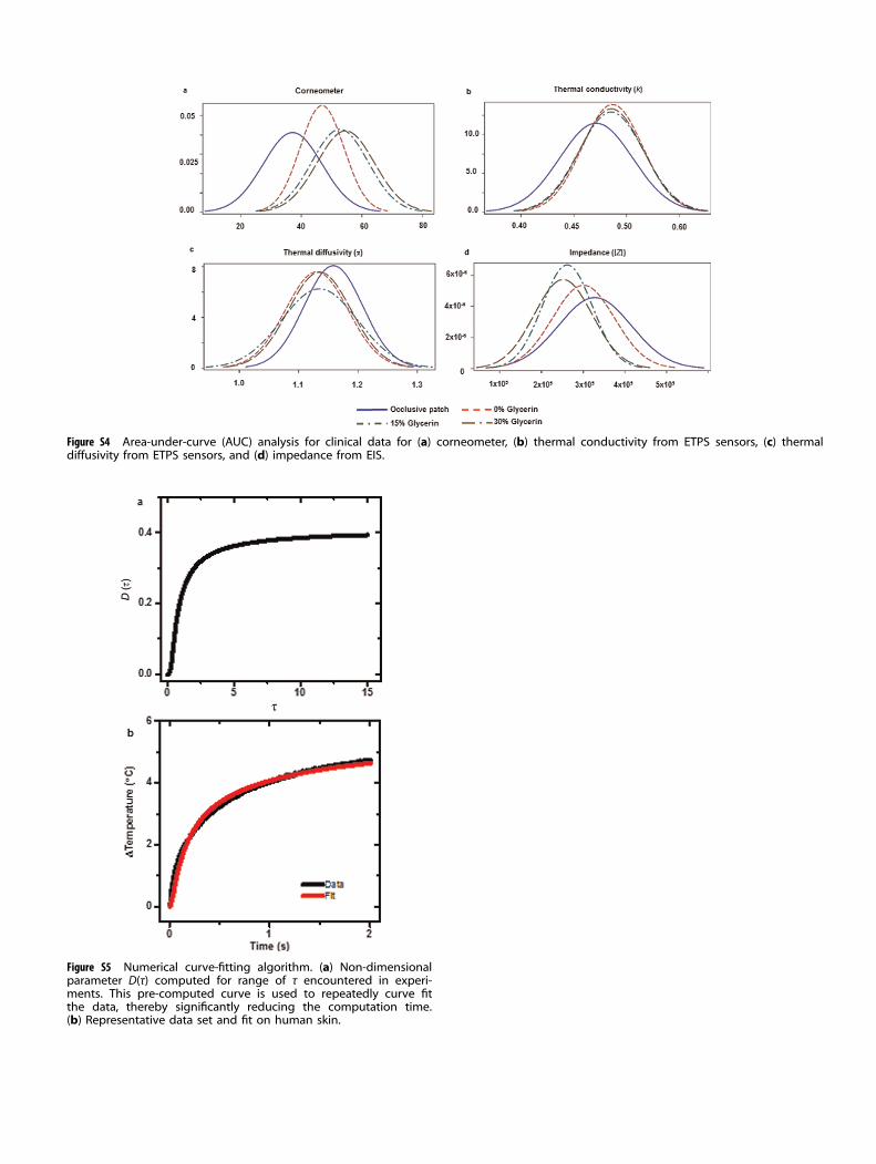
Figure S4 Area-under-curve (AUC) analysis for clinical data for (a) corneometer, (b) thermal conductivity from ETPS sensors, (c) thermaldiffusivity from ETPS sensors, and (d) impedance from EIS.

Figure S5 Numerical curve-fitting algorithm. (a) Non-dimensionalparameter D(τ) computed for range of τ encountered in experi-ments. This pre-computed curve is used to repeatedly curve fitthe data, thereby significantly reducing the computation time.(b) Representative data set and fit on human skin.

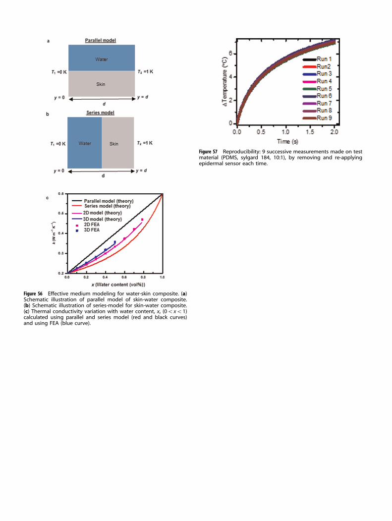
Figure S6 Effective medium modeling for water-skin composite. (a)Schematic illustration of parallel model of skin-water composite.(b) Schematic illustration of series-model for skin-water composite.(c) Thermal conductivity variation with water content, x, (0oxo1)calculated using parallel and series model (red and black curves)and using FEA (blue curve).

Figure S7 Reproducibility: 9 successive measurements made on testmaterial (PDMS, sylgard 184, 10:1), by removing and re-applyingepidermal sensor each time.