supplementary information for “efficient bayesian … · supplementary information for...
TRANSCRIPT

Supplementary Information for “Efficient Bayesian mixed modelanalysis increases association power in large cohorts”
Po-Ru Loh, George Tucker, Brendan K Bulik-Sullivan, Bjarni J Vilhjalmsson, Hilary K Finucane,Rany M Salem, Daniel I Chasman, Paul M Ridker, Benjamin M Neale, Bonnie Berger,
Nick Patterson, Alkes L Price
Contents
Supplementary Note 3
1 BOLT-LMM algorithm details 31.1 Model setup . . . . . . . . . . . . . . . . . . . . . . . . . . . . . . . . . . . . . . 3
1.1.1 Initialization: Missing data, normalization, and covariates . . . . . . . . . 31.1.2 Models . . . . . . . . . . . . . . . . . . . . . . . . . . . . . . . . . . . . 41.1.3 Estimated SNP effect sizes . . . . . . . . . . . . . . . . . . . . . . . . . . 8
1.2 Variance component estimation: Monte Carlo REML approximation . . . . . . . . 101.2.1 Conjugate gradient iteration to solve mixed model equations . . . . . . . . 13
1.3 Gaussian mixture model fitting: Variational Bayes iteration . . . . . . . . . . . . . 131.4 Cross-validation for estimating Gaussian mixture parameters . . . . . . . . . . . . 141.5 LD Score regression . . . . . . . . . . . . . . . . . . . . . . . . . . . . . . . . . 151.6 Performance optimization . . . . . . . . . . . . . . . . . . . . . . . . . . . . . . . 16
1.6.1 Memory . . . . . . . . . . . . . . . . . . . . . . . . . . . . . . . . . . . . 161.6.2 Computational speed . . . . . . . . . . . . . . . . . . . . . . . . . . . . . 17
2 Theory 192.1 Variational Bayes . . . . . . . . . . . . . . . . . . . . . . . . . . . . . . . . . . . 19
2.1.1 Terminology and notation . . . . . . . . . . . . . . . . . . . . . . . . . . 192.1.2 General variational iteration . . . . . . . . . . . . . . . . . . . . . . . . . 212.1.3 Variational iteration for Bayesian linear regression . . . . . . . . . . . . . 222.1.4 Update equations for Gaussian mixture prior . . . . . . . . . . . . . . . . 242.1.5 Equivalence with penalized linear regression . . . . . . . . . . . . . . . . 27
2.2 Convergence rate of BOLT-LMM iterative computations . . . . . . . . . . . . . . 302.3 Correspondence between association power and prediction accuracy . . . . . . . . 31
3 Parameters of mixed model software used in analyses 32
4 Pseudocode outlining BOLT-LMM algorithm 33
1
Nature Genetics: doi:10.1038/ng.3190

5 Data sets 385.1 Simulations . . . . . . . . . . . . . . . . . . . . . . . . . . . . . . . . . . . . . . 38
5.1.1 Simulated genotypes . . . . . . . . . . . . . . . . . . . . . . . . . . . . . 385.1.2 Simulated phenotypes . . . . . . . . . . . . . . . . . . . . . . . . . . . . 385.1.3 LD Scores for simulated data . . . . . . . . . . . . . . . . . . . . . . . . . 39
5.2 WGHS data . . . . . . . . . . . . . . . . . . . . . . . . . . . . . . . . . . . . . . 39
Supplementary Figures 46
Supplementary Tables 53
2
Nature Genetics: doi:10.1038/ng.3190

1 BOLT-LMM algorithm details
The BOLT-LMM algorithm is overviewed in Online Methods. Here, we provide additional details
for components of the computation not fully described earlier.
1.1 Model setup
1.1.1 Initialization: Missing data, normalization, and covariates
Given a data set of genotypes and phenotypes, we apply the following procedure to create a nor-
malized genotype matrix X . We begin by dealing with missing data as follows. First, we perform
QC by filtering out SNPs and individuals with missing rates exceeding thresholds (default 10%
for each). Second, we filter out individuals with missing phenotypes. Third, if the analysis in-
cludes covariates, we filter out individuals with any missing covariates. (As an alternative to this
approach, known as “complete case analysis,” we also implement the option to use the “missing
indicator method,” which adds missing status indicator variables as additional covariates.) Finally,
we replace missing genotypes in the remaining data with per-SNP averages. We denote by N and
M the numbers of samples and SNPs remaining post-QC.
Next, we mean-center each SNP and normalize the SNPs to have equal sample variance. We
also mean-center the phenotypes. We model covariates by projecting them out from both genotypes
and phenotypes, which is equivalent to including them as fixed effects. Explicitly, we compute a
basis spanning the covariate vectors and subtract out the components of the SNP and phenotype
vectors along the basis vectors. This procedure is mathematically equivalent to multiplying by
an orthogonal projection matrix Pfixed that projects vectors to an (N − C)-dimensional subspace
S ⊂ RN orthogonal to the covariates, where C is the number of independent covariates (including
the all-1s vector, which is implicitly included as a covariate upon mean-centering). For compar-
ison, GCTA-LOCO [12] version 1.24 provides two options for treating covariates: (1) projecting
out covariates from the phenotype vector only (the default, which is an approximate approach);
or (2) fitting covariates as fixed effects along with the candidate SNP in each association test (the
--mlma-no-adj-covar option, which is equivalent to projecting covariates out from both geno-
types and phenotypes). The GCTA-LOCO documentation notes that the latter option significantly
reduces the computational efficiency of GCTA-LOCO, but the BOLT-LMM implementation is not
3
Nature Genetics: doi:10.1038/ng.3190

subject to this loss of computational efficiency.
We denote by X the final N × M matrix of genotypes and y the final N -vector of pheno-
types after QC, normalization, and projection. While y and all columns of X (i.e., SNP vectors)
are N -dimensional vectors, it is important to keep in mind that they all actually belong to the
(N − C)-dimensional subspace S left after projecting by Pfixed. For example, when estimating
variance parameters, accounting for the loss of degrees of freedom distinguishes restricted max-
imum likelihood (REML) analysis—the preferred approach, which we implement—from maxi-
mum likelihood (ML), and when computing χ2 test statistics, we need to use N − C instead of N
as the sample size.
1.1.2 Models
We therefore use the following general model to estimate hyperparameters (i.e., variance param-
eters under the infinitesimal model and Gaussian mixture parameters under the non-infinitesimal
model):
y = Xβ + eproj, (18)
where
y ∈ S ⊂ RN : projected phenotypes
X = N ×M matrix, xm ∈ S ⊂ RN for m = 1, . . . ,M : projected genotypes
β ∈ RM : iid random effects with E[βm] = 0,Var(βm) = σ2β
eproj ∈ S ⊂ RN : iid random normal noise with eproj ∼ N(0, σ2ePfixed).
Reiterating the point above, this “mixed” model does not contain any fixed effects; the fixed effects
have been projected out, so that the entire model—including the noise term eproj—lives in the
subspace S.
Model for estimating infinitesimal model parameters. When estimating variance parameters
under the infinitesimal model in Step 1a of the BOLT-LMM algorithm, we assume the SNP effect
4
Nature Genetics: doi:10.1038/ng.3190

prior is the normal distribution
βm ∼ N(0, σ2β)
and we estimate σ2β and σ2
e using the stochastic REML approximation algorithm described in Sec-
tion 1.2. Note that the following notation is often used for the total genetic effect Xβ and its
covariance:
g = Xβ
K =XX ′
M(the “empirical kinship” or GRM)
σ2gK = Cov(g)
in which case
σ2β = σ2
g/M.
Model for estimating Gaussian mixture model parameters. When estimating Gaussian mix-
ture parameters in Step 2a of the BOLT-LMM algorithm (after having obtained estimates of σ2g and
σ2e in Step 1a), we generalize the SNP effect prior to the three-parameter mixture of normals
βm ∼
N(0, σ2β,1) with probability p
N(0, σ2β,2) with probability 1− p,
(19)
where we require
pσ2β,1 + (1− p)σ2
β,2 = σ2β = σ2
g/M.
We reparameterize the remaining two degrees of freedom using the parameters f2 and p, where
f2 denotes the proportion of the total mixture variance within the second Gaussian (the “spike”
component that models small genome-wide effects):
f2 =(1− p)σ2
β,2
pσ2β,1 + (1− p)σ2
β,2
.
Thus, Step 2a consists of estimating f2 and p.
5
Nature Genetics: doi:10.1038/ng.3190

Prospective model for computing association statistics. When performing association tests
(under the infinitesimal model) in Step 1b of the BOLT-LMM algorithm, we modify the above
models by (1) including the SNP being tested as a fixed effect and (2) leaving out all SNPs on its
chromosome from the random effect:
y = xtestβtest +XLOCOβ + eproj. (20)
As discussed in Online Methods, we do not by default re-estimate the hyperparameters σ2g , σ
2e
(and f2, p in the Gaussian mixture case; see below) when performing association tests; instead,
we simply reuse the estimates obtained above from the slightly different models above, which
include all SNPs in the random effect (and no fixed effect). However, we also offer the option of
re-estimating σ2g and σ2
e with each chromosome left out in turn.
Retrospective formulation of association tests. In Online Methods, we defined the BOLT-
LMM-inf χ2 test statistic as an approximation of the standard prospective mixed model χ2 statistic
using the model of equation (20). We then briefly noted that the BOLT-LMM-inf association test
can also be viewed as a retrospective quasi-likelihood score test similar to T SCORE−R [44] and
MASTOR [23]. Following ref. [23], this viewpoint models the phenotype y as known and the SNP
xtest as random, being drawn from a distribution with covariance Cov(xtest) = Φ and mean
E[xtest | y] = (ΦV −1y)α, (21)
where we wish to test the null hypothesis α = 0. Note that xtest is a discrete random variable,
so we cannot formally model it as a multivariate normal and perform likelihood-based analysis,
but the retrospective mean model is enough to obtain a quasilikelihood score test statistic that is
asymptotically χ2-distributed:
χ2LMM-R =
(xtestΦ−1(ΦV −1y))2
(ΦV −1y)′Φ−1(ΦV −1y)=
(xtestV−1y)2
(V −1y)′Φ(V −1y). (22)
Previous formulations of this statistic [23, 44] have been aimed at family studies in which the
pedigree matrix may be used as the covariance matrix Φ. For the general case of individuals with
6
Nature Genetics: doi:10.1038/ng.3190

unknown pedigree, a seemingly natural choice is to substitute the GRM, but unfortunately, the
GRM does not accurately reflect the covariance matrix of the distribution of unassociated (i.e.,
null) SNPs, which form the null model under the retrospective framework. In particular, for large
sample sizes, this approach incurs deflation because it incorporates SNPs associated with y into the
covariance model (for xtest, treated as random), causing overestimation of the variance of xtestV−1y.
This phenomenon is not overcome by LOCO analysis because unlike with prospective modeling,
the problem is not proximal contamination; rather, it is polygenicity: to obtain unbiased variance
estimates based on genotype data, we would need to eliminate associated SNPs, which runs into
the same difficulty faced by genomic control [13, 24].
While the denominator of χ2LMM-R in equation (22), (V −1y)′Φ(V −1y), cannot be computed
without Φ (which is in general inaccessible as discussed above), it does not involve the candidate
SNP xtest and can therefore be treated as a constant calibration factor, so that in practice, equation
(22) is equivalent to the BOLT-LMM-inf formulation in equation (8). (More precisely, within
a LOCO scheme, the matrix V depends on which chromosome xtest belongs to, so there should
formally be a different denominator for each chromosome, but all are approximately equal.) The
retrospective model thus provides an alternative justification for the BOLT-LMM-inf statistic.
Importantly, the retrospective viewpoint also enables a natural generalization of BOLT-LMM-
inf to the more powerful BOLT-LMM association test for non-infinitesimal phenotypes. The basic
observation motivating this extension is that in the retrospective mixed model statistic χ2LMM-R,
the vector V −1y is a scalar multiple of the residual after best linear unbiased prediction (BLUP)—
i.e., the component of the phenotype remaining after conditioning out SNP effects estimated by the
mixed model, which drives the power of mixed model association—but this vector may be replaced
by any other vector not involving xtest. More precisely, we generalize the infinitesimal retrospective
mean model, equation (21), by replacing the BLUP residual σ2eV−1y with the residual phenotype
yresid-LOCO upon conditioning out the effects of SNPs not on the same chromosome as xtest (where
yresid-LOCO is estimated by fitting a Gaussian mixture extension of the standard LMM):
E[xtest | y] = (Φyresid-LOCO)α. (23)
This model produces χ2BOLT-LMM as a quasi-likelihood score test for α ?
= 0.
7
Nature Genetics: doi:10.1038/ng.3190

1.1.3 Estimated SNP effect sizes
When performing a genome-wide association study, it is of interest not only to analyze χ2 statistics
for association but also estimated SNP effect sizes; to this end, BOLT-LMM outputs such effect
sizes. We explain below how BOLT-LMM estimates effect sizes, but first, we discuss an important
distinction between two uses of the term “estimated effect size” that can be a source of confusion.
Distinction between estimated effect sizes in association tests vs. prediction. When perform-
ing mixed model GWAS, each SNP xm is in turn tested for association with the phenotype y, and
the “estimated effect size” of xm is defined to be the fitted value βm,assoc of the fixed effect xm in the
mixed model given by equation (20), taking xtest = xm. Importantly, the model in equation (20) is
different for each SNP, with the fixed effect xm changing from test to test (and the SNPs included
in the random effect also changing from chromosome to chromosome, assuming the LOCO frame-
work is being used). If we denote the (estimated) phenotypic covariance by V−chr(m), the mixed
model association effect size is given by
βm,assoc =x′mV
−1−chr(m)y
x′mV−1−chr(m)xm
. (24)
Note that equation (24) is very similar to but not the same as the formula for the prospective mixed
model test statistic:
χ2m =
(x′mV−1−chr(m)y)2
x′mV−1−chr(m)xm
. (25)
(We also note in passing that the BLUP residual is given by σ2eV−1y, which is why the standard
mixed model association test is similar to testing the SNP for correlation with the BLUP residual.)
In contrast, when performing mixed model prediction (i.e., BLUP), a single model is fit, equa-
tion (18), in which all SNPs are included as random effects. Each SNP receives an “estimated
effect size” when the model is fit, but these effect sizes,
βm,BLUP =σ2g
Mx′mV
−1y, (26)
are conceptually completely different from the association effect size estimates βm,assoc. The ef-
fect sizes βm,BLUP are meaningful precisely for the purpose of prediction; that is, they have the
8
Nature Genetics: doi:10.1038/ng.3190

property that building a linear combination of the SNPs using the coefficients βm,BLUP produces
the BLUP prediction. In particular, these coefficients take into account linkage disequilibrium
between nearby SNPs to correctly weight their contributions. These same statements apply to the
effect sizes that BOLT-LMM iterates on internally when using variational Bayes to fit the Bayesian
mixed model.
For a concrete example that may aid intuition, consider two SNPs in perfect LD. When testing
association, each SNP should be ignored when testing the other; the fact that we happen to have
two redundant tags should not change the strength of association. However, when creating a risk
score (i.e., prediction), it would be incorrect to assign each SNP the effect size assuming only
one copy of the SNP: doing so would overweight the contribution of these SNPs. Instead, the LD
needs to be accounted for by acknowledging the presence of both SNPs and splitting the total effect
between the two SNPs.
To summarize, we emphasize that association effect sizes must not be confused with predic-
tion effect sizes; in particular, it is inappropriate to use the former as coefficients for polygenic
prediction.
Estimated effect sizes reported by BOLT-LMM. Estimating association effect sizes—i.e., βm,assoc
given in equation (24)—is computationally challenging for the same reasons that computing χ2 as-
sociation statistics in equation (25) is challenging: building and inverting the covariance matrix is
slow. Fortunately, it turns out that we can harness that fact that we already have a way to estimate
χ2 statistics: namely, BOLT-LMM-inf. Combining equations (24) and (25), we have
βm,assoc =x′mV
−1−chr(m)y
x′mV−1−chr(m)xm
=χ2m
x′mV−1−chr(m)y
≈χ2m,BOLT-LMM-inf
x′mV−1−chr(m)y
. (27)
BOLT-LMM already computes both the statistics χ2m,BOLT-LMM-inf and the quantities V −1−chr(m)y, so
the final expression in equation (27) is simple to compute. This quantity is the effect size estimate
that the BOLT-LMM software reports. (Note that the BOLT-LMM software reports this effect size
regardless of whether the infinitesimal or Gaussian mixture prior is used because there is no natural
analog of the above for the Gaussian mixture model.)
9
Nature Genetics: doi:10.1038/ng.3190

1.2 Variance component estimation: Monte Carlo REML approximation
Here we provide details of our stochastic algorithm for estimating REML variance parameters in
Step 1a of BOLT-LMM. The crux of the method is to employ the observation that the REML
first-order conditions on σ2g and σ2
e are equivalent [48, equation (14.8)] to the system of equations
E[∑
e2rand] =∑
e2data, E[∑
β2rand] =
∑β2
data, (28)
where both the left and right sides of each equation, defined below, are functions of the assumed
variance parameters σ2g and σ2
e . (The summations are over components of each vector, which is a
slight abuse of notation for ||e||2 and ||β||2.)
• On the right sides, edata and βdata are best linear unbiased predictions (BLUP) on the observed
phenotype data assuming the basic linear mixed model y = Xβ + eproj, equation (18), with
Cov(y) = σ2g
XX ′
M+ σ2
ePfixed.
• On the left sides, expectations are taken over the same quantities, with the phenotype data
replaced by random yrand generated according to the model y = Xβ + eproj with variance
parameters set to the assumed σ2g and σ2
e .
We can therefore estimate the left sides (for a particular choice of σ2g and σ2
e ) by Monte Carlo sam-
pling, i.e., by generating random yrand = Xβrand + erand from βrand,m ∼ N(0, σ2g/M), erand,n ∼
N(0, σ2e) and then performing BLUP on yrand—i.e., solving the mixed model equations (Sec-
tion 1.2.1)—using the assumed σ2g and σ2
e [26, 27]. Only a few Monte Carlo trials are required;
BOLT-LMM computes 3–15 trials, with the number of trials decreasing as N increases, reflecting
the way in which the standard error depends on sample size and the number of trials. Explicitly,
BOLT-LMM by default uses 4 × 10⁹/N2 trials, with a minimum of 3 and a maximum of 15. The
number of trials can also be varied as a user-specified parameter.
Explicitly, defining
δ = σ2e/σ
2g (29)
H =XX ′
M+ δIN , (30)
10
Nature Genetics: doi:10.1038/ng.3190

the BLUP estimates β and e for a phenotype vector y are:
β =1
MX ′H−1y (31)
e = δH−1y. (32)
(Note that technically, the scaled covariance matrix is actually HS = σ2gCov(y) = XX′
M+ δPfixed;
however, because all of our vectors belong to the subspace S, using IN instead of Pfixed produces
the correct result and has the convenience of making the operator H invertible in the full space
RN .)
Equations (29)–(32) show that for a fixed value of δ, the BLUP predictions e and β are constant.
Thus, the right sides of the REML first order conditions (28), involving BLUP on the observed
phenotypes, depend only on the variance ratio δ and are independent of the variance scale, which
we may parameterize by σ2g (in which case σ2
e = σ2gδ becomes a dependent variable). The left
sides scale proportionately with σ2g because scaling up the variances scales up randomly generated
phenotypes yrand. Therefore, finding σ2g and σ2
e that solve the pair of equations (28) is equivalent
to: (1) finding the value of the single parameter δ such that
E[∑β2]
E[∑e2]
=
∑β2
data∑e2data
, (33)
and (2) choosing σ2g to scale the expectations to match the values observed on the data. (This
procedure is analogous to the usual REML trick of optimizing over δ and then setting σ2g =
y′H−1y/(N − C) [49].)
We propose an algorithm that rapidly estimates the ratio of expectations in equation (33) and
uses this estimate within a one-parameter search over δ. Define
fREML(log δ) = log
(∑β2
data∑e2data
/E[∑β2]
E[∑e2]
).
For a fixed value of δ, we produce Monte Carlo estimates of the expectations by generating random
phenotypes
yrand = Xβrand + erand, proj,
11
Nature Genetics: doi:10.1038/ng.3190

where
βrand ∼ iid N(
0,√
1/M)
erand ∼ iid N(0,√δ)
erand, proj = Pfixederand.
(Note that as the variance scale parameter σ2g is irrelevant for this part of the computation, we set
it to 1 for convenience. Note also that the use of the projection matrix Pfixed is what makes this
procedure compute REML rather than ML estimates.) We then run BLUP (using the chosen value
of δ) using conjugate gradient iteration [28, 29] (Section 1.2.1) to obtain Monte Carlo estimates of
E[∑β2]/E[
∑e2], and we likewise run BLUP to compute βdata and edata, which together give an
estimate fREML(δ) of fREML(δ).
We wish to find δ such that fREML(log δ) = 0. We have observed empirically in simulations
and real data sets that fREML(log δ) increases monotonically with δ except possibly at extremely
small or large values of δ outside the range of reasonable parameter values (corresponding to, say,
0.01 < hg2< 0.99). Thus, one approach to finding the unique zero of fREML within the reasonable
parameter range is binary search, with the caveat that some care is needed because we can only
compute noisy Monte Carlo estimates fREML of fREML.
We implement the following more robust approach. Instead of independently re-randomizing
phenotypes yrand used to compute estimates fREML at different values of δ, we a generate a single
set of random phenotypic component pairs
βrand ∼ N(
0,√
1/M)
erand, unscaled ∼ N(0, 1)
erand, unscaled, proj = Pfixederand, unscaled
and then use these component pairs to generate random phenotypes
yrand = Xβrand +√δ · erand, unscaled, proj.
12
Nature Genetics: doi:10.1038/ng.3190

for any given δ. Using this approach (taken in ref. [26]), the Monte Carlo estimate fREML(log δ)
becomes a smooth function of log δ, allowing us to use the secant method, a finite difference
approximation of Newton’s method, to perform zero-finding on fREML.
We note that satisfying the first-order conditions is not in general a sufficient condition to have
found the REML global optimum, but for the case of only one non-identity variance component,
the likelihood surface appears to be well-behaved, and we have never observed an instance in
which this estimation procedure failed.
1.2.1 Conjugate gradient iteration to solve mixed model equations
The core computational subroutine needed for Monte Carlo REML (and also for calibration of the
BOLT-LMM-inf statistic) is solution of the mixed model equations, i.e., computation of expres-
sions of the form V −1x, where
V = σ2g
XX ′
M+ σ2
eIN .
We solve the mixed model equations using conjugate gradient iteration as in refs. [28, 29], which
requires onlyO(MN )-time matrix-vector products. More precisely, computing V −1x using conju-
gate gradient iteration only requires computing products of V with vectors, which we can compute
in O(MN )-time without forming V by leaving V in factored form σ2gXX
′/M +σ2eIN , distributing
the product, and multiplying from right to left. Note that V is positive definite because XX ′ is
positive semidefinite and σ2g , σ
2e > 0. Moreover, because most real phenotypes have only a small
fraction of heritable variance, the identity component σ2eIN typically accounts for much of the
covariance V , so that V is a well-conditioned matrix and conjugate gradient iteration converges
rapidly (as determined by the residual norm dropping below a specified relative tolerance, which
by default we set to 0.0005).
1.3 Gaussian mixture model fitting: Variational Bayes iteration
As outlined in Online Methods, the core component of the BOLT-LMM Gaussian mixture mod-
eling algorithm is a variational iteration [20–22, 38] that computes approximate posterior mean
effect sizes βm for the Gaussian mixture model version of equation (18). We sketch the iteration
in slightly more detail here, leaving a full description for Section 2.
13
Nature Genetics: doi:10.1038/ng.3190

The idea of the iteration is to obtain successively better approximations of the SNP effect sizes
by cyclically updating each estimated SNP effect with its posterior mean conditional on the current
estimates of all other SNP effects. Explicitly, we begin by initializing each SNP effect βm to 0 and
initializing the residual phenotype yresid = y−Xβ to y. Then, each iteration performs the following
loop over SNPs m = 1, . . . ,M :
1. Remove effect of SNP m from residual. yresid,−m ← yresid + xmβm
2. Re-estimate effect of SNP m. βm ← posterior mean given yresid,−m
3. Replace effect of SNP m in residual. yresid ← yresid,−m − xmβm
Step 2 amounts to computing the posterior mean of βm given its assumed mixture prior in equa-
tion (19), the environmental noise distribution eproj ∼ N(0, σ2ePfixed), and the residual phenotype
yresid,−m given current estimates of all other SNP effects. Steps 1 and 3 are a computational tech-
nique allowing the residual in Step 2 not to be computed from scratch for each SNP, so that an
entire iteration (updating each SNP effect once) takes O(MN) time.
The basic structure of this iteration is the shared with previous variational methods [20–22,38],
with the update Step 2 varying among methods depending on the assumed SNP effect prior. As
noted in Online Methods, an additional slight difference is that BOLT-LMM estimates the hyperpa-
rameters σ2g , σ2
β using REML and f2, p using cross-validation [15], whereas previous approaches
have performed hyperparameter estimation within the variational iteration [22, 38] or using the
variational approximate log likelihood [21]. We used cross-validation instead because we found
cross-validation estimates to be more robust to decreases in the quality of the variational approxi-
mation caused by linkage disequilibrium.
1.4 Cross-validation for estimating Gaussian mixture parameters
BOLT-LMM performs model selection among the 18 possible parameter pairs (f2, p) by perform-
ing cross-validation to optimize mean-squared prediction R2. More precisely, for each parameter
pair, for each cross-validation fold, BOLT-LMM estimates posterior mean SNP effect sizes βm
on the training data and uses these effect size estimates to make predictions on the left-out fold,
which are then compared to the actual left-out phenotype values. (Note that effect size estimates
used as coefficients in genomic prediction are conceptually completely different from effect sizes
14
Nature Genetics: doi:10.1038/ng.3190
output by an association test, as discussed in Section 1.1.3.) The parameter pair (f2, p) producing
the highest prediction R2 (mean across folds) is then selected. However, if the best model only
reduces prediction error by less than 1% (in absolute prediction R2) compared to the infinitesimal
model, BOLT-LMM terminates the Gaussin mixture analysis and does not proceed to Step 2b to
compute association statistics. We implement this feature as the default option to save unnecessary
computation in situations where the Gaussian mixture model provides little or no improvement in
association power.
We perform 5-fold cross-validation to select best-fit Gaussian mixture model parameters ac-
cording to maximal prediction R2. For large sample sizes N > 10,000, computing a subset of the
cross-validation folds is already sufficient to obtain parameter estimates that achieve near-optimal
association power, so by default, we compute only enough folds to make predictions on 10,000 test
fold samples. This observation holds because absolute prediction R2 corresponds directly to the
power of the corresponding retrospective association test (as measured by increase in χ2 statistics
at truly associated loci, or equivalently, increase in effective sample size; see Online Methods), and
the standard error of prediction R2 estimated via cross-validation scales as the inverse square root
of the number of test samples.
1.5 LD Score regression
LD Score regression [24] observes that for complex traits, properly calibrated χ2 association statis-
tics approximately obey the following linear trend (on average across the genome):
χ2 ∼ 1 + (constant) · (LD Score), (34)
where loosely speaking, the LD Score of the test SNP is its effective number of LD partners.
Because the intercept of this regression relation is 1, it follows that if we have computed a set
of χ2 statistics up to an unknown constant factor c, then one way to estimate c is to compute the
intercept of the regression of χ2 statistics on LD Scores. (Note that this approach only works on
test statistics that are not vulnerable to proximal contamination; equation (34) does not hold for
χ2 statistics that are deflated due to LD between the candidate SNP and SNPs included in the
model.)
15
Nature Genetics: doi:10.1038/ng.3190

To achieve very precise calibration, BOLT-LMM adopts a slightly more complex procedure
that matches the intercept of LD Score regression on χ2BOLT-LMM (after calibration) to that of the
properly-calibrated infinitesimal statistic χ2BOLT-LMM-inf. We do so to increase robustness of the
calibration to violations of the modeling assumptions underlying LD Score regression, which
may result in attenuation bias (i.e., inflation of the intercept toward the mean χ2) that causes
the straightforward LD Score correction to association statistics to be conservative, though still
much less conservative than genomic control. Because LD Score regression on either χ2BOLT-LMM
or χ2BOLT-LMM-inf should be affected roughly equally by attenuation bias, matching LD intercepts
guards against this potential problem (Supplementary Table 6).
1.6 Performance optimization
Beyond the broad algorithmic techniques we have described, the BOLT-LMM software employs a
variety of performance optimizations that provide large constant-factor savings (>10x) in memory
and running time over a straightforward implementation.
1.6.1 Memory
Computation on raw genotypes. The key optimization that we implement for memory effi-
ciency is direct computation on raw genotypes. Raw genotypes can be stored in only 2 bits per
base, versus 64 bits (8 bytes) for standard double-precision floating point values. However, all pre-
vious methods necessarily work with floating point matrices (either the N ×N GRM or a floating
point representation of the N × M normalized genotype matrix) because they perform spectral
decomposition. In contrast, because BOLT-LMM applies iterative methods that use the genotype
matrix only in matrix multiplications, it is enough for us to store the raw genotypes plus lookup
tables containing normalization information that we apply on-the-fly. Explicitly, for each SNP,
rather than storing a normalized genotype vector in memory, we simply store its raw allele count
(0, 1, 2, or missing) for each individual and additionally record its mean allele count and normal-
ization constant. Then, when performing computations involving the SNP, we build a properly
normalized SNP vector using the above information. Importantly, this vector can be thrown away
after the computation, thus keeping BOLT-LMM’s memory footprint small.
16
Nature Genetics: doi:10.1038/ng.3190

An additional subtlety arises when working with covariates because normalized genotype vec-
tors no longer contain only 4 values after projecting out covariates. In this case, we store the
components of each normalized genotype vector along a basis that spans the covariates, and we
do the same for the phenotype vector. We treat these “covariate component” values as additional
coordinates that we carry along in all computations, so that whenever we need to compute a dot
product (the basic computation all of our iterations use), we can do so by taking the usual dot
product and subtracting the dot product of the additional covariate component vector.
Streaming computation of association tests. In analyses of data sets containing very large num-
bers of SNPs (e.g., millions of imputed SNPs) that may be stored as real-valued dosages, it is often
desirable to compute association statistics for all SNPs but use only a subset of genotyped SNPs
in the mixed model. In this situation, we retain memory efficiency by reading and analyzing SNPs
not used in the mixed model only when performing final computation of retrospective association
test statistics. That is, we first compute a set of residual phenotypes yresid-LOCO using only the sub-
set of typed SNPs in the model; then, we successively read each test SNP and compute and output
its association test, throwing away the SNP after completing the computation. This streaming
computation allows us never to store the full set of SNPs in memory.
1.6.2 Computational speed
Batch computation using optimized matrix subroutines. The iterative methods we have de-
scribed reduce the association computation to basic building blocks of vector operations (for vari-
ational iteration) and matrix-vector operations (for conjugate gradient iteration). These operations
can be performed using optimized implementations of the Basic Linear Algebra Subprograms
(BLAS), but all BLAS libraries achieve maximal speed when performing matrix-matrix “Level 3
BLAS” operations. We therefore batch our computations into matrix-matrix multiplications by
performing simultaneous updates across SNPs and parameter values.
Conjugate gradient iteration uses Level 2 BLAS operations as written. Variational iteration
only uses Level 1 BLAS as written (Section 1.3), so to step up to Level 2 BLAS, we perform block
updates of SNP effect sizes. Explicitly, the basic variational iteration consists of re-estimating each
SNP effect in turn conditioned on current estimates of other SNP effects, which requires computing
17
Nature Genetics: doi:10.1038/ng.3190
dot products of each SNP with the residual phenotype vector. Instead of computing dot products
one at a time (a Level 1 BLAS operation), we compute dot products of a block of 64 SNPs at once
(a matrix-vector multiplication, which is Level 2 BLAS). When we subsequently update the effect
size of each SNP in turn, we just need to be careful to update its dot product to reflect changes that
have been made to the residual vector due to previous updates of previous SNPs within the block.
We do so by precomputing a 64 × 64 correlation matrix for each SNP block.
To step up from Level 2 BLAS to Level 3 BLAS, we make use of the fact that all computation-
ally intensive steps of the BOLT-LMM algorithm require multiple replicates of almost the same
computation: Step 1a computes BLUP on different random phenotypes; Step 1b solves a set of
similar linear systems for different LOCO reps and calibration SNPs; Step 2a computes variational
Bayes assuming different hyperparameter values; Step 2b computes variational Bayes for different
LOCO reps. With some care, we can in each case simultaneously perform iterations across the
different replicates. The upshot is that by using batch computations, BOLT-LMM performs all
O(MN )-time operations using BLAS 3 matrix-matrix multiplications (DGEMM). Our software
distribution uses the well-tuned Intel Math Kernel Library (MKL) BLAS implementation.
Multithreading. Conveniently, most BLAS implementations also support optimized multithreaded
computation on multi-core processors, which are now commonplace. In practice, multithreading
rarely decreases computation time by a factor equal to the number of cores used because of vari-
ous overhead costs, but Level 3 BLAS operations often come close to achieving this theoretically
maximal speedup. The BOLT-LMM software supports multithreading through BLAS, and we rec-
ommend using this option whenever multiple cores are available. We performed our benchmarking
analyses using single-core computation simply to give a fair comparison against methods that do
not support multithreading.
Low-level optimization. We reduce the overhead of loading raw genotypes and building normal-
ized genotype vectors using a few additional low-level tricks. Instead of looking up normalized
genotype values one at a time when loading a SNP, we build an intermediate lookup table that maps
all 256 possible values of 4 consecutive genotypes (stored in 1 byte) to a 4-vector of normalized
values. When loading these 4-vectors from the lookup table into the normalized SNP vector being
18
Nature Genetics: doi:10.1038/ng.3190

built, we use streaming SIMD extensions (SSE instructions) to perform multiple loads at once.
2 Theory
2.1 Variational Bayes
In Bayesian analysis, one specifies a probability model over observations and model parameters,
often wishing to obtain posterior mean estimates of parameters of interest. Unfortunately, the
posterior distribution is typically infeasible to integrate over. The idea of the variational framework
(termed “variational Bayes”) is to approximate the posterior distribution with a factorized form that
is much easier to work with computationally. The factorized form can be integrated over, allowing
calculation of approximate posterior mean estimates. For a full discussion of variational Bayes,
we refer to ref. [50]. Previous variational methods for Bayesian linear regression in genetics have
been presented in refs. [21,22,38]. Here, we briefly summarize key aspects of variational Bayes for
quick reference and to establish notation. We then derive formulas giving the variational iteration
used by BOLT-LMM, and we further derive theory establishing equivalence between this family
of variational methods and penalized linear regression.
2.1.1 Terminology and notation
We begin by considering a general probability model p(y, β) over observations y and parameters
β. We assume that p(y, β) takes into account the prior distributions of β, so that p(y, β) is the joint
probability of sampling parameters β and observing y.
• The true log likelihood (LL) of observing y is the log of the integral of p(y, β) over all
possible values of the parameters β:
true LL = log
∫p(y, β)dβ.
This integral is typically intractable to compute.
• The true posterior distribution of the parameters β conditional on observing y is given by
19
Nature Genetics: doi:10.1038/ng.3190

normalizing the joint probability p(y, β) by the likelihood:
true posterior distribution = p(β | y) =p(y, β)∫p(y, β)dβ
.
• The variational approximation to the posterior distribution is the best approximation of the
posterior distribution p(β | y) with a distribution q(β) that factors:
approx posterior distribution = q(β) =∏i
qi ≈ p(β | y).
The factors qi are usually constrained to have simple forms. For instance, if β represents
a set of individual parameters βi, each factor qi may be required to be a function of only
one parameter βi, in which case qi is an approximate marginal posterior for βi. This fully
factorized variational approximation is the approach we consider here.
• The approximate log likelihood is a variational lower bound on the true log likelihood, given
by:
approx LL = L(q) =
∫q(β) log
p(y, β)
q(β)dβ (35)
= true LL−DKL(q(β) ‖ p(β | y)),
whereDKL denotes the Kullback-Liebler (KL) divergence between probability distributions.
Note that the second line says that the gap between the variational lower bound and the true
LL is given by the KL divergence between the approximating distribution q and the true
posterior distribution p(β | y).
Variational iteration, which we describe in the next section, successively refines the approxi-
mation of p(β | y) with q(β) by iteratively updating the factors qi, reducing the KL divergence
DKL(q(β) ‖ p(β | y)) and therefore monotonically improving the lower bound L(q). The point
of the iteration is that at convergence, the distribution q(β) will ideally be a good approximation
of the true posterior distribution p(β | y) that can easily be integrated over (because of its factored
form) to perform approximate posterior inference.
20
Nature Genetics: doi:10.1038/ng.3190

Before moving on, we note that it follows from the above that the faithfulness of the approx-
imating distribution q(β) to the true posterior p(β | y) determines the accuracy of the resulting
approximate posterior inference. Because we only consider approximating distributions q(β) that
factor as∏
i qi, the optimal quality of the approximation depends on the extent to which the pos-
terior distribution p(β | y) can be approximately factored in the prescribed manner. For Bayesian
linear regression, which is our focus here, correlation among regressors (i.e., linkage disequilib-
rium among markers) tends to pose a challenge for some types of inference using variational meth-
ods. For example, when regressors are correlated, the approximate posterior is often too tightly
concentrated (i.e., overconfident of parameter localization). However, aggregate inference can still
be robust. We refer to ref. [21] for an in-depth exploration of these issues.
2.1.2 General variational iteration
The variational Bayes algorithm iteratively updates each approximate marginal distribution qi using
the update step
log(qi(βi))← Eqi′ , i′ 6=i[log p(y, β)] + C.
As written, the above update step updates the entire distribution qi—a function of βi—to its new
optimum (as a distribution, optimizing in the sense of calculus of variations). Indeed, the only
assumption made by the variational approximation is that the approximate posterior distribution
q(β) factors (i.e., the parameters are assumed to be conditionally independent, conditional on the
observed outputs): no assumption is made about the functional form of the factors qi(βi). However,
the factor distributions qi are typically characterized by sets of sufficient statistics, so that in each
iteration, only the sufficient statistics for factor i need to be updated based on the current values
of the sufficient statistics for each of the other factors. Moreover, we will show in Section 2.1.3
that in the case of Bayesian linear regression, the factor distributions take the form of conditional
posterior distributions. For the Gaussian mixture priors we use in BOLT-LMM, these conditional
posteriors retain the Gaussian mixture form, just with different parameters.
Convex optimization theory guarantees the convergence of variational iteration [45]. Moreover,
convergence of the approximate log likelihood, which monotonically increases during the iteration,
serves as a convergence criterion. At convergence, approximate posterior means of the parameters
21
Nature Genetics: doi:10.1038/ng.3190

βi can be read off from the approximate marginal distributions qi: for the special case of fully
factorized Bayesian linear regression, these values are among the sufficient statistics updated at
each iteration.
2.1.3 Variational iteration for Bayesian linear regression
We now specialize to the Bayesian linear regression model
y = Xβ + e
e ∼ N(0, σ2eIN)
prior on βm = πm(βm)
That is, we assume each regression coefficient (i.e., SNP effect) has a prior distribution πm(βm) and
the response y is the sum of regressor effects plus iid Gaussian noise with variance σ2e . (Note that
this noise model does not take into account projecting out covariates as described in Section 1.1;
projecting out C independent covariates just reduces N to N − C in the equations below.) The
joint probability p(y, β) of parameters β and observations y satisfies
p(y, β) = pnoise(y −Xβ)∏
πm(βm) =
(1√
2πσ2e
)N
exp
(−||y −Xβ||
2
2σ2e
) M∏m=1
πm(βm). (36)
Below we derive the fact that the fully factorized variational approximation matches the it-
erative conditional update algorithm discussed in Section 1.3. The fully factorized variational
approximation takes the form
q(β) =M∏m=1
qm(βm) ≈ p(β | y).
The variational update step for the approximate marginal distribution qm optimizes the KL diver-
gence DKL(q||p) over all distributions qm, fixing the other marginals qm′ to their current distribu-
tions, thereby monotonically increasing the approximate (lower bound) log likelihood L(q). The
22
Nature Genetics: doi:10.1038/ng.3190

update amounts to:
log(qm(βm)) ← Eqm′ (βm′ ), m′ 6=m[log p(y, β)] + C
= Eqm′ (βm′ ), m′ 6=m
[−||y −Xβ||
2
2σ2e
+M∑
m′=1
log πm′(βm′)
]+ C
= −||y −X−mβ−m − xmβm||2
2σ2e
+ log πm(βm) + C
= −||yresid,−m − xmβm||2
2σ2e
+ log πm(βm) + C,
where β−m denotes the vector of estimated posterior mean effect sizes at SNPs other than m
according to the current approximate marginal posterior distributions qm′(βm′). (In the above se-
quence of equations, we absorb all terms independent of βm into the constant C; the use of “+C”
in all lines does not imply that the constant is the same from line to line.) To see how the posterior
mean estimates β−m enter the equation in the third line above, consider expanding the quadratic
term ||y −Xβ||2 inside the expectation. (Note that taking an expectation over qm′(βm′), m′ 6= m
corresponds to integrating over qm′(βm′)dβm′ .)
• For terms that are linear in βm′ (for m′ 6= m), E[βm′ ] can be replaced with βm′ by linearity
of expectation over qm′(βm′).
• Terms that are quadratic in βm′ are independent of βm, so E[β2m′ ] can be replaced by β
2
m′ +
Varqm′ (βm′) to re-complete the square ||y − X−mβ−m − xmβm||2. The leftover terms, pro-
portional to Varqm′ (βm′) = Eqm′ [β2m′ ] − β
2
m′ , are constant (with respect to βm) and can be
absorbed into the constant term.
Finally, the contributions of the prior terms πm′(βm′) for m′ 6= m also become additive constants
upon taking expectations and can be absorbed into the constant term as well.
Exponentiating the result above gives
qm(βm) ∝ exp
(−||yresid,−m − xmβm||2
2σ2e
)πm(βm), (37)
which is simply a conditional posterior distribution for βm (given the prior πm(βm) and conditional
on setting all other βm′ to their variational expected means). That is, for Bayesian linear regression,
23
Nature Genetics: doi:10.1038/ng.3190
the optimal approximating marginal distribution q(βm) (making no assumptions about the form of
each marginal, only requiring that the approximating posterior fully factorizes) turns out to be the
conditional posterior. In particular, as we derive in Section 2.1.4, if the prior has the nice form of
a mixture of Gaussians, then the approximating marginal keeps that form (with different means,
standard deviations, and weights).
Moreover, the approximate log likelihood L(q) can be obtained by substituting the joint prob-
ability p(y, β) = pnoise(y −Xβ)∏πm, given in equation (36), into equation (35):
L(q) =
∫q(β) log
p(y, β)
q(β)dβ
= Eq[log pnoise(y −Xβ)] +∑
Eq[log πm/qm]
= Eq[log pnoise(y −Xβ)]−∑
DKL(qm||πm)
= −N2
log 2πσ2e −||y −Xβ||2
2σ2e
−∑||xm||2Varqm(βm)
2σ2e
−∑
DKL(qm||πm)
= −N2
log 2πσ2e −||y −Xβ||2
2σ2e
−∑||xm||2Varqm(βm)
2σ2e
+∑
(Eqm [log πm] +H(qm)),
(38)
where βm = Eqm [βm], using the same trick of completing the square as above, only now we have
to be careful to account for the leftover constant terms involving Varqm(βm). In the last line,H(qm)
denotes information entropy. Once again, we note that if C independent covariates are projected
out from our model as described in Section 1.1, then we simply reduce N to N − C in equation
(38) to account for the lost degrees of freedom.
2.1.4 Update equations for Gaussian mixture prior
We now specialize to Bayesian linear regression with the specific Gaussian mixture prior
βm ∼
N(0, σ2β,1) with probability p
N(0, σ2β,2) with probability 1− p,
(39)
24
Nature Genetics: doi:10.1038/ng.3190

i.e.,
πm(βm) = p · 1√2πσ2
β,1
exp
(− β2
m
2σ2β,1
)+ (1− p) · 1√
2πσ2β,2
exp
(− β2
m
2σ2β,2
).
To obtain the the conditional marginal distribution qm(βm), we substitute the above into equation
(37), obtaining
qm(βm) = pm ·1√
2πτ 2m,1
exp
(−
(βm − βm,1)2
2τ 2m,1
)+ (1−pm) · 1√
2πτ 2m,2
exp
(−
(βm − βm,2)2
2τ 2m,2
),
i.e.,
βm ∼qm
N(βm,1, τ
2m,1
)with probability pm
N(βm,2, τ
2m,2
)with probability 1− pm,
where
βm :=yTresid,−mxm
||xm||2
βm,k :=σ2β,k
σ2β,k + (σ2
e/||xm||2)βm
τ 2m,k :=1
1σ2e/||xm||2
+ 1σ2β,k
=σ2β,kσ
2e/||xm||2
σ2β,k + (σ2
e/||xm||2)
pm :=
ps1e−β
2m/2s
21
ps1e−β
2m/2s
21 + 1−p
s2e−β
2m/2s
22
where s21 and s22 are the variances of the marginal distribution of βm in each case (assuming
yresid,−m = xmβm + e and marginalizing over random βm and e):
s2k := σ2β,k +
σ2e
||xm||2
for k = 1, 2. These equations explicitly give the update formulas for the BOLT-LMM variational
iteration (Step 2 in Section 1.3), in which each estimated SNP effect is set to its conditional poste-
rior mean.
To compute the approximate log likelihood for use in testing convergence of the iteration, it is
convenient to consider a reparameterization of the model (following ref. [21]) in which instead of
25
Nature Genetics: doi:10.1038/ng.3190

having one parameter βm for each SNP (with πm(βm) a mixture of two Gaussians), we introduce
a state parameter sm ∈ {0, 1} and consider a prior πm(βm, sm) with:
πm(βm | sm = 0) = Gaussian 1: N(0, σ2β,1)
πm(βm | sm = 1) = Gaussian 2: N(0, σ2β,2)
πm(sm = 0) = mixture fraction: p.
This parameterization gives exactly the same model as the original Bayesian linear regression, with
the only difference being that the mixture prior on βm in equation (39) is replaced by the joint prior
distribution πm(βm, sm) above with the extra hidden state sm.
We can now apply the variational approach to factorize the approximate posterior distribution
over all SNPs—in (βm, sm) pairs—as a product of joint distributions qm(βm, sm). Each optimal
factor distribution qm has the property that when integrated over sm, it matches the variational
approximation qm(βm) from the original parameterization, implying that the estimated posterior
means are identical. This parameterization lends itself more easily to computation of KL diver-
gences, however. We have the formula:
DKL(qm(βm) ‖ πm(βm)) = DKL(qm(βm, sm) ‖ πm(βm, sm))
= pm logpmp
+ (1− pm) log1− pm1− p
− pm2
(1 + log
τ 2m,1σ2β,1
−τ 2m,1 + β
2
m,1
σ2β,1
)
− 1− pm2
(1 + log
τ 2m,2σ2β,2
−τ 2m,2 + β
2
m,2
σ2β,2
).
Writing
Varqm(βm) = Eqm [β2m]− β2
m = pm(τ 2m,1 + β2
m,1) + (1− pm)(τ 2m,2 + β2
m,2)− β2
m,
we have all of the terms needed to compute L(q) according to equation (38).
We note that in the limit σβ,2 → 0 of the point-normal prior used by ref. [21], the formulas
26
Nature Genetics: doi:10.1038/ng.3190

become
DKL(qm(βm) ‖ πm(βm)) = pm logpmp
+ (1− pm) log1− pm1− p
− pm2
(1 + log
τ 2m,1σ2β,1
−τ 2m,1 + β
2
m,1
σ2β,1
)Varqm(βm) = pm(τ 2m,1 + β
2
m,1)− β2
m
= pm(τ 2m,1 + β2
m,1)− (pmβm,1)2,
matching ref. [21].
2.1.5 Equivalence with penalized linear regression
We now show that the variational iteration of Section 2.1.3 for Bayesian linear regression is equiv-
alent to coordinate descent applied to a penalized linear regression problem. Equivalently, the fully
factorized variational approximation to Bayesian linear regression (for an arbitrary choice of prior
on regressor effects) can be recast as applying a transformation to the prior and then finding a
posterior mode of the (new) Bayesian linear regression with transformed prior. More precisely, we
have the following equivalence of optimization problems:
1. Maximize the variational approximate log likelihood (for the fully factored VB approxima-
tion to Bayesian linear regression).
2. Minimize the penalized linear regression objective function
||y −Xβ||2 +∑
penaltym(βm),
where the penalty is derived from the prior in the original Bayesian linear regression.
3. Find a posterior mode of the Bayesian linear regression with prior
πm(βm) ∝ exp(−penaltym(βm)),
which we can view as a transformation of the original prior πm(βm).
27
Nature Genetics: doi:10.1038/ng.3190

We also have the following equivalence of algorithms:
1. Variational iteration applied to the original Bayesian linear regression.
2. Coordinate descent applied to the corresponding penalized linear regression.
Implications for numerical optimization. The equivalence of variational Bayes with penalized
linear regression (in the context of Bayesian linear regression) elucidates some numerical proper-
ties of the algorithm that are not immediately apparent. In particular, penalized linear regression is
in general a numerically challenging non-convex optimization. We can therefore expect variational
iteration to be susceptible to numerical issues such as convergence to local optima. Some methods
have tried to address this problem by repeating the iteration for different random choices of update
orders or different initialization points [21,22,38]. In our simulations, we found that using a single
run of the iteration was typically already sufficient for BOLT-LMM to achieve most of the avail-
able power gain, however, so we opted to use just a single run to avoid increasing computational
cost.
Mathematical derivation. As discussed in Section 2.1.1, variational theory gives the following
lower bound to the log likelihood, which variational iteration tries to maximize:
L(q) = −N2
log 2πσ2e −||y −
∑xmEqm [βm]||2
2σ2e
−∑||xm||2Varqm(βm)
2σ2e
−∑
DKL(qm||πm).
Note that L(q) is a functional, i.e., it evaluates factored distributions q = q1 · · · qM that attempt to
approximate the posterior. We will show that in fact, this maximization is equivalent to optimizing
the objective function (over effect size estimates βm) of a penalized linear regression:
L(β) = −N2
log 2πσ2e −||y −Xβ||2
2σ2e
−∑
penaltym(βm).
The key is that we can define a mapping βm 7→ qm( · ; βm) with Eqm [βm] = βm and define
penaltym(βm) :=||xm||2Var(qm( · ; βm))
2σ2e
+∑
DKL(qm( · ; βm)||πm),
28
Nature Genetics: doi:10.1038/ng.3190

with the property that
(penalized LR objective) L(β) = L(q =
∏qm( · ; βm)
)(approx LL with derived qm)
≤ max{L(q) : q =
∏qm, Eqm [βm] = βm
}(40)
≤ maxL(q). (41)
(Note that if the SNPs are normalized such that ||xm|| are all equal, then the penalty is independent
of m.)
The mapping βm 7→ qm( · ; βm) is derived from the variational update step, which we know
chooses the qm that optimizes L(q) conditional on the current choices of the other marginal dis-
tributions. Thus, equality holds in (40) at any convergence “point” of the iteration. Here a con-
vergence “point” really means a choice of approximating distributions q1, . . . , qM ; however, if the
above mapping exists, these distributions may be parameterized by β1, . . . , βM . Equality holds
in (41) at the global maximizer of the variational approximate log likelihood. It follows that
L(β), which is upper-bounded by the global maximum of L(q), attains that global maximum at
βm,opt = Eqm,opt [βm]. That is, the solution to the penalized linear regression optimization of L(β)
corresponds to the solution to the variational optimization of L(q): if we could solve the penalized
linear regression optimally, we would have the optimal variational Bayes solution.
All that remains is to define the mapping βm 7→ qm( · ; βm), which we obtain indirectly from
the variational update step via the key observation that the optimal marginal qm conditioned on
all other marginals depends only on a single statistic: the correlation of xm with the residual
yresid,−m = y −∑
m′ 6=m xm′Eqm′ [βm′ ]. That is, we have:
xTmyresid,−m 7→ qm 7→
penalty terms Var(qm), DKL(qm||πm)
conditional posterior mean Eqm [βm]
Moreover, the conditional posterior mean Eqm [βm] is an increasing function of the correlation
statistic xTmyresid,−m, meaning that we can invert the final mapping to obtain Eqm [βm] 7→ qm, giving
the desired mapping βm 7→ qm(·; βm). If we wanted to derive an explicit formula for penaltym(βm),
we could try to invert the mapping xTmyresid,−m 7→ Eqm [βm], but in general there is probably no
closed form.
29
Nature Genetics: doi:10.1038/ng.3190

2.2 Convergence rate of BOLT-LMM iterative computations
Because BOLT-LMM applies iterative methods for numerical linear algebra, its running time de-
pends not only on the cost of matrix operations, which scales linearly with M and N , but also
the number of O(MN )-time iterations required for convergence, which is largely determined by
the condition number of the phenotypic covariance matrix and in particular increases with sample
size (N ), heritability, relatedness, and population structure. Simulations show empirically that the
number of iterations scales roughly with√N and does not change dramatically within the range
of typical values of the other parameters, hence our estimate of an overall running time that scales
roughly with MN 1.5 (Supplementary Fig. 1 and Supplementary Fig. 2).
More precisely, we measured (for varying N ) the numbers of iterations required by BOLT-
LMM-inf and BOLT-LMM to reach convergence, as defined by: (1) the conjugate gradient resid-
ual norm dropping below a relative tolerance of 0.0005, in BOLT-LMM-inf; and (2) the variational
Bayes change in approximate log likelihood dropping below 0.01, in BOLT-LMM. For both meth-
ods, we observed that the number of iterations increased roughly as√N (Supplementary Fig. 1).
For BOLT-LMM-inf, our intuition (based on random matrix theory) is that the conditioning of
the covariance matrix becomes modestly worse as the sample size increases; we believe this phe-
nomenon is responsible for the ≈√N increase in conjugate gradient iterations. For BOLT-LMM,
which faces a nonlinear problem due to its Gaussian mixture prior on effect sizes, we are not aware
of theoretical bounds on the convergence rate of variational iteration. However, the nonlinearity
appears not to be a major hurdle in practice, perhaps because heritability is typically low and also
because we limit the nonlinearity by bounding the extent to which the mixture prior deviates from
normality (by bounding the mixture parameters f2 and p).
We note that the high observed-scale heritabilities of case-control ascertained traits and inflated
heritabilities of phenotypes in family data, in combination with population structure or relatedness
among samples, may reduce the computational efficiency of BOLT-LMM (Supplementary Fig. 2);
an avenue for future investigation is to mitigate this effect by including PCs to improve the numer-
ical conditioning of the computation.
30
Nature Genetics: doi:10.1038/ng.3190

2.3 Correspondence between association power and prediction accuracy
Intuitively, mixed model analysis to test a candidate marker for association gains power over lin-
ear regression (assuming no confounding) by conditioning on other markers modeled as random
effects. This intuition is especially clear in the BOLT-LMM statistical formulation, where we ret-
rospectively test candidate markers for association with residual phenotypes. Residualizing elim-
inates the component of phenotype that was successfully predicted by other markers, so that the
subsequent association test is trying to detect candidate marker association signal amid phenotypic
variance (“noise”) that has been decreased by a factor of 1-R2. (Here, R2 denotes out-of-sample
prediction R2; even though in practice we residualize by genetic predictions computed in-sample,
the extent to which these predictions capture true genetic effects corresponds to out-of-sample
prediction R2.) Note that residualizing leaves the amount of candidate marker signal unchanged,
assuming no proximal contamination and assuming a randomly ascertained phenotype; violation
of these assumptions results in loss of power [12].
Quantitatively, a reduction of association test noise by a factor of 1-R2 results in an increase
in χ2 statistics by a factor of 1/(1-R2) at truly associated loci. (More precisely, the quantity χ2-1
increases by 1/(1-R2) on average, but for χ2 � 1 at known loci, this distinction is minor.) This
relationship can be seen explicitly in comparing equation (1) of ref. [34] for prediction R2 using
BLUP,
R2 =h2g
1 + MNh2g
(1−R2), (42)
with Supplementary Table 2 of ref. [12], which gives the following formulas for mean χ2 statistics
using linear regression vs. mixed model association:
mean χ2LR at causal SNPs = 1 +
Mh2gM causal
(43)
mean χ2LMM at causal SNPs = 1 +
Mh2gM causal
· 1
1−R2, (44)
where R2 in equation (44) (denoted r2h2g in ref. [12]) satisfies the same quadratic equation (42).
In Fig. 3a, we plot increases in mean χ2 statistics at known loci for mixed model methods
vs. PCA, and in Fig. 3b, we plot absolute prediction R2. As explained above, the increase in
mean χ2 statistics at known loci for mixed model methods vs. linear regression—assuming no
31
Nature Genetics: doi:10.1038/ng.3190

confounding—is approximately 1/(1 − R2) − 1 ≈ R2. When including principal components in
linear regression to avoid confounding, we get an increase in mean χ2 statistics at known loci for
mixed model methods vs. PCA of approximatelyR2LMM−R2
PCA, where the latter is the prediction
R2 obtained by linear prediction using only the principal components. Thus, the red bars in Fig. 3a
roughly correspond to differences between red and black bars in Fig. 3b, and analogously for
blue bars. The correspondence is approximate because of the approximations mentioned above
and two additional subtleties: (1) the LOCO scheme that BOLT-LMM uses to avoid proximal
contamination renders the mixed model unable to condition out effects of markers on the same
chromosome as the candidate marker; (2) our measurement of prediction R2 uses 5-fold cross-
validation, reducing the training sample size by 20%. However, these two effects have small
magnitudes and act in opposite directions, so that ultimately the correspondence is very tight, as is
visually apparent in Fig. 3.
We note two caveats to the correspondence between association power and prediction accuracy
claimed above. First, in ascertained case-control data sets, mixed model methods that achieve pos-
itive prediction R2 may actually reduce association power due to ascertainment-induced “linkage
disequilibrium” between causal markers [12]. The result of this phenomenon is that residualizing
by other SNPs has a deleterious, masking effect on the association signal at a candidate SNP, sim-
ilar to proximal contimation [5, 9, 12]. Second, in data sets with pervasive family relatedness, the
correspondence between association power and prediction accuracy is again less clear-cut. Our
intuition here is similar: family relatedness introduces “long-range LD” that produces an effect
similar to proximal contamination.
3 Parameters of mixed model software used in analyses
We ran BOLT-LMM with default options except in analyses investigating power of the Gaussian
mixture model, in which we used the --forceNonInf option to fit the Gaussian mixture model
even in scenarios with no expected power gain.
We ran the 2012-02-10 intel64 release of EMMAX with default options. We ran GEMMA
version 0.94 with default options. We ran GCTA version 1.24 with the --mlma-loco option
for leave-one-chromosome-out analysis. We ran FaST-LMM version 2.07 using all markers to
32
Nature Genetics: doi:10.1038/ng.3190

compute the similarity matrix. We ran FaST-LMM-Select version 2.07 with the autoSelect option
-autoSelectSearchValues
"0,1,3,10,30,100,300,1000,3000,10000,30000,100000,300000"
to test increasing numbers of selected SNPs up to a maximum of 300,000 SNPs. We benchmarked
the precompiled executable distribution of each software package.
4 Pseudocode outlining BOLT-LMM algorithm
Step 1a: Estimate variance parameters.Algorithm: Use secant iteration to find approximate zero of derivative of log likelihood.
X := normalized genotypes # N x M matrix
y := phenotype vector # N-vector
MCtrials := max(min(4e9/N2, 15), 3) # set number of Monte Carlo trials
for t = 1 to MCtrials
for j = 1 to M
βrand[j,t] := randn() * sqrt(1/M) # generate random SNP effects
for i = 1 to N
erand,unscaled[i,t] := randn() # generate random environmental effects
end for
h21 := 0.25, logDelta1 := log((1-h2
1)/h21)
f1 := evalfREML(logDelta1) # perform first fREML evaluation
if f1 < 0, h22 := 0.125; else h2
2 := 0.5
logDelta2 := log((1-h22)/h
22)
f2 := evalfREML(logDelta2) # perform second fREML evaluation
for s = 3 to 7 # perform up to 5 steps of secant iteration
logDeltas := (logDeltas−2*fs−1 - logDeltas−1*fs−2) / (fs−1 - fs−2)
if abs(logDeltas - logDeltas−1) < 0.01 # check convergence
break
fs := evalfREML(logDeltas) # perform next fREML evaluation
end for
33
Nature Genetics: doi:10.1038/ng.3190

return σ2g := y′H−1y/N, σ2
e := δ * σ2g
###
function f = evalfREML(logDelta)
for t = 1 to MCtrials
# build random phenotypes using pre-generated components
yrand[:,t] := X * βrand[:,t] +√δ * erand,unscaled[:,t]
# compute H−1yrand[:,t], where H = XX’/M+δI
H−1yrand[:,t] := conjugateGradientSolve(X, δ, yrand[:,t])
# compute BLUP estimated SNP effect sizes and residuals
βrand[:,t] := 1/M * X’ * H−1yrand[:,t]
erand[:,t] = δ * H−1yrand[:,t]
end for
# compute BLUP estimated SNP effect sizes and residuals for real phenotypes
H−1ydata := conjugateGradientSolve(X, δ, y)
βdata[:,t] := 1/M * X’ * H−1ydata[:,t]
edata[:,t] = δ * H−1ydata[:,t]
# evaluate fREML
f := log((sum(β2data) / sum(e2data)) / (sum(β2
rand) / sum(e2rand)))
end
Step 1b: Compute and calibrate BOLT-LMM-inf statistics.
σ2g,σ
2e := variance parameters calculated in Step 1a
# precompute V −1-chry, where V-chr = σ2gX-chrX-chr’/M-chr + σ2
eI
for chr = 1 to 22
V −1-chry := conjugateGradientSolve(X-chr, σ2g, σ2
e, y)
end for
# compute calibration for BOLT-LMM-inf statistic using 30 random SNPs
34
Nature Genetics: doi:10.1038/ng.3190

for t = 1 to 30
m := random SNP in {1..M}
x := X[:,m] # normalized genotype vector for chosen SNP m
chr := chromosome containing chosen SNP m
V −1-chrx := conjugateGradientSolve(X-chr, σ2g, σ2
e, x)
prospectiveStat[t] := (x’V −1-chry)ˆ2/(x’V−1-chrx)
uncalibratedRetrospectiveStat[t] := N * (x’V −1-chry)2/(norm(x)2
*norm(V−1-chry)
2)
end for
infStatCalibration := sum(uncalibratedRetrospectiveStats) / sum(prospectiveStats)
# compute BOLT-LMM-inf mixed model statistics at all SNPs
for m = 1 to M
x := X[:,m]
chr := chromosome containing SNP m
boltLMMinf[m] := N * (x’V −1-chry)ˆ2/(norm(x)2*norm(V
−1-chry)
2) / infStatCalibration
end for
return boltLMMinf[:]
35
Nature Genetics: doi:10.1038/ng.3190

Step 2a: Estimate Gaussian mixture prior parameters.Algorithm: Optimize prediction mean-squared error in cross-validation.
σ2g,σ
2e := variance parameters calculated in Step 1a
for f2 in {0.5, 0.3, 0.1}
for p in {0.5, 0.2, 0.1, 0.05, 0.02, 0.01}
MSE[f2,p] := 0
for CVfold in 1 to 5
foldIndivs := subset of samples {1..N} in fold CVfold
Xtrain := X[-foldIndivs,:], ytrain = y[-foldIndivs]
Xtest := X[foldIndivs,:], ytest = y[foldIndivs]
[βfit,yresid] := fitVariationalBayes(Xtrain,ytrain,σ2g,σ
2e,f2,p)
ypred := Xtest * βfit
MSE[f2,p] += norm(ypred - ytest)2
end for
end for
end for
return [f2,p] = argmin(MSE)
###
function [βfit,yresid] = fitVariationalBayes(X,y,σ2g,σ
2e,f2,p)
σ2β,1 := σ2
g/M * (1-f2) / p # set Gaussian variances
σ2β,2 := σ2
g/M * f2 / (1-p)
βfit := zero M-vector # initialize SNP effect estimates to 0
yresid := y # initialize residual phenotype to y
approxLL := -inf
for t = 1 to maxIters # perform VB iterations until convergence or maxIters
approxLLprev := approxLL
approxLL := -N/2 * log(2πσ2e)
# update SNP effect estimates in turn and accumulate contributions to approxLL
for m = 1 to M
x := X[:,m]
yresid += βfit[m] * x # remove effect of SNP m from residual
βm := x’ * yresid / norm(x)2 # see formulas in 2.1.4
36
Nature Genetics: doi:10.1038/ng.3190

βfit[m] := pm * βm,1 + (1-pm) * βm,2 # set effect size to conditional posterior mean
approxLL -= norm(x)2/(2σ2e) * Varqm(βm) + DKL(qm||πm) # update approxLL (see 2.1.4)
yresid -= βfit[m] * x # update residual with new effect of SNP m
end for
approxLL -= norm(yresid)2 / (2σ2e)
# test convergence
if approxLL - approxLLprev < 0.01
break
end for
end
Step 2b: Compute and calibrate BOLT-LMM Gaussian mixture model statistics.
σ2g,σ
2e,f2,p := mixture parameter estimates from Steps 1b and 2a
boltLMMinf[:] := infinitesimal mixed model stats computed in Step 1b
# compute uncalibrated BOLT-LMM statistics
for chr in 1 to 22 # leave-one-chromosome-out (LOCO) to avoid proximal contamination
# fit model using all SNPs not on chromosome; compute residuals
[βfit,yresid] := fitVariationalBayes(X-chr,y,σ2g,σ
2e,f2,p)
for m in (SNPs on chr)
uncalibratedBoltLMM[m] := N * (X[:,m]’yresid)2 / (norm(X[:,m])2*norm(yresid)
2)
end for
end for
# calibrate BOLT-LMM statistics using LD Score
interceptBoltLMMinf := LDscoreIntercept(boltLMMinf) # see LD Score ref. [24]
interceptUncalibratedBoltLMM := LDscoreIntercept(uncalibratedBoltLMM)
LDscoreCalibration := interceptUncalibratedBoltLMM / interceptBoltLMMinf
# apply calibration
for m in 1 to M
boltLMM[m] := uncalibratedBoltLMM[m] / LDscoreCalibration
end for
return boltLMM[:]
37
Nature Genetics: doi:10.1038/ng.3190

5 Data sets
5.1 Simulations
We simulated data sets from the WTCCC2 data with the goal of creating realistic test scenarios
including linkage disequilibrium and possible confounding from population stratification or relat-
edness. The WTCCC2 data set contains 15,633 samples genotyped at 360,557 SNPs after QC; full
details are given in ref. [12]. In the simulations that we ran to assess power and Type I error, we
used these genotypes directly (subsampling to N = 5,211 samples for some simulations).
5.1.1 Simulated genotypes
In the simulations we used to benchmark computational costs, we simulated genotype data with
N = 3,750 to 480,000 individuals and M = 150,000 or 300,000 SNPs by subsampling the desired
number of SNPs from the WTCCC2 data set and then independently building N individuals as
mosaics of individuals from the original data set using the following procedure. First, specify a
number of “ancestors” A for each individual to have. Then, for each simulated individual, select
A ancestors at random from among the original individuals and create the simulated individual’s
genotype data by chopping the genome into segments of 1,000 SNPs and copying each segment
from a randomly sampled (diploid) ancestor.
Note that this approach retains realistic LD among SNPs, and for small values of A, it also
retains population structure and introduces relatedness among individuals that share ancestors. In
our simulations, we used A = 2 (substantial structure and relatedness) or A = 10 (low levels of
structure and relatedness).
5.1.2 Simulated phenotypes
We simulated phenotypes as sums of up to four components: genetic effects from a specified
number of causal SNPs, genetic effects from a specified number of standardized effect SNPs, pop-
ulation stratification, and environmental effects. We simulated genetic effects by selecting SNPs
at random from the first half of the list of typed SNPs in each chromosome and at least 2Mb and
2cM before the middle SNP. (Likewise, when assessing calibration at null SNPs, we only tested
38
Nature Genetics: doi:10.1038/ng.3190

SNPs in the second halves of chromosomes and at least 2Mb and 2cM beyond the middle SNP, to
avoid contamination of null SNPs from LD with causal SNPs.) We sampled effect sizes for the
selected normalized SNPs from a standard normal distribution. We simulated population strati-
fication by taking the first principal component of the normalized genotype matrix. We sampled
environmental effects for all individuals from a standard normal. To create phenotypes with speci-
fied proportions of variance explained by each of these effects, we normalized each component (an
N -vector across samples) and created a linear combination of the components with weights equal
to the square roots of the desired variance fractions. Note that standardized effect SNPs thus have
effect sizes that vary from SNP to SNP; it is the average variance explained by these SNPs that is
standardized.
5.1.3 LD Scores for simulated data
Because causal SNPs in our simulated phenotypes are selected only from among genotyped SNPs,
we computed reference LD Scores (used to calibrate the BOLT-LMM statistic in our simulations)
by summing LD only to typed SNPs—as opposed to all SNPs, which is appropriate for real phe-
notypes [24]—in 379 European-ancestry samples from the 1000 Genomes Project [51].
5.2 WGHS data
The Women’s Genome Health Study (WGHS) is a prospective cohort of initially healthy, female
North American health care professionals at least 45 years old at baseline representing participants
in the Women’s Health Study (WHS) who provided a blood sample at baseline and consent for
blood-based analyses. The WHS was a 2x2 trial beginning in 1992-1994 of vitamin E and low
dose aspirin in prevention of cancer and cardiovascular disease with about 10 years of follow-
up. Since the end of the trial, follow-up has continued in observational mode. Genotyping in the
WGHS sample was performed using the HumanHap300 Duo “+” chips or the combination of the
HumanHap300 Duo and iSelect chips (Illumina, San Diego, CA) with the Infinium II protocol.
For quality control, all samples were required to have successful genotyping using the BeadStudio
v. 3.3 software (Illumina, San Diego, CA) for at least 98% of the SNPs. A subset of 23,294 indi-
viduals were identified with self-reported European ancestry that could be verified on the basis of
39
Nature Genetics: doi:10.1038/ng.3190

multidimensional scaling analysis of identity by state using 1443 ancestry informative markers in
PLINK v. 1.06. In the final data set of these individuals, a total of 339,596 SNPs were retained with
MAF >1%, successful genotyping in 90% of the subjects, and deviations from Hardy-Weinberg
equilibrium not exceeding p = 10−6 in significance. In our analyses, we further eliminated non-
autosomal SNPs, duplicate SNPs, and custom SNPs, leaving 324,488 SNPs.
40
Nature Genetics: doi:10.1038/ng.3190

References1. Yu, J. et al. A unified mixed-model method for association mapping that accounts for
multiple levels of relatedness. Nature Genetics 38, 203–208 (2006).
2. Kang, H. M. et al. Efficient control of population structure in model organism associationmapping. Genetics 178, 1709–1723 (2008).
3. Kang, H. M. et al. Variance component model to account for sample structure in genome-wide association studies. Nature Genetics 42, 348–354 (2010).
4. Zhang, Z. et al. Mixed linear model approach adapted for genome-wide association studies.Nature Genetics 42, 355–360 (2010).
5. Lippert, C. et al. FaST linear mixed models for genome-wide association studies. NatureMethods 8, 833–835 (2011).
6. Zhou, X. & Stephens, M. Genome-wide efficient mixed-model analysis for associationstudies. Nature Genetics 44, 821–824 (2012).
7. Segura, V. et al. An efficient multi-locus mixed-model approach for genome-wide associa-tion studies in structured populations. Nature Genetics 44, 825–830 (2012).
8. Korte, A. et al. A mixed-model approach for genome-wide association studies of correlatedtraits in structured populations. Nature Genetics 44, 1066–1071 (2012).
9. Listgarten, J. et al. Improved linear mixed models for genome-wide association studies.Nature Methods 9, 525–526 (2012).
10. Svishcheva, G. R., Axenovich, T. I., Belonogova, N. M., van Duijn, C. M. & Aulchenko,Y. S. Rapid variance components-based method for whole-genome association analysis.Nature Genetics (2012).
11. Listgarten, J., Lippert, C. & Heckerman, D. FaST-LMM-Select for addressing confoundingfrom spatial structure and rare variants. Nature Genetics 45, 470–471 (2013).
12. Yang, J., Zaitlen, N. A., Goddard, M. E., Visscher, P. M. & Price, A. L. Advantages andpitfalls in the application of mixed-model association methods. Nature Genetics 46, 100–106 (2014).
13. Yang, J. et al. Genomic inflation factors under polygenic inheritance. European Journal ofHuman Genetics 19, 807–812 (2011).
14. Stahl, E. A. et al. Bayesian inference analyses of the polygenic architecture of rheumatoidarthritis. Nature Genetics 44, 483–489 (2012).
15. Lippert, C. et al. The benefits of selecting phenotype-specific variants for applications ofmixed models in genomics. Scientific Reports 3 (2013).
41
Nature Genetics: doi:10.1038/ng.3190
16. Rakitsch, B., Lippert, C., Stegle, O. & Borgwardt, K. A Lasso multi-marker mixed modelfor association mapping with population structure correction. Bioinformatics 29, 206–214(2013).
17. Meuwissen, T., Hayes, B. & Goddard, M. Prediction of total genetic value using genome-wide dense marker maps. Genetics 157, 1819–1829 (2001).
18. de los Campos, G., Hickey, J. M., Pong-Wong, R., Daetwyler, H. D. & Calus, M. P. Whole-genome regression and prediction methods applied to plant and animal breeding. Genetics193, 327–345 (2013).
19. Zhou, X., Carbonetto, P. & Stephens, M. Polygenic modeling with Bayesian sparse linearmixed models. PLoS Genetics 9, e1003264 (2013).
20. Meuwissen, T., Solberg, T. R., Shepherd, R. & Woolliams, J. A. A fast algorithm for BayesBtype of prediction of genome-wide estimates of genetic value. Genet Sel Evol 41 (2009).
21. Carbonetto, P. & Stephens, M. Scalable variational inference for Bayesian variable selectionin regression, and its accuracy in genetic association studies. Bayesian Analysis 7, 73–108(2012).
22. Logsdon, B. A., Hoffman, G. E. & Mezey, J. G. A variational Bayes algorithm for fastand accurate multiple locus genome-wide association analysis. BMC Bioinformatics 11, 58(2010).
23. Jakobsdottir, J. & McPeek, M. S. MASTOR: mixed-model association mapping of quanti-tative traits in samples with related individuals. American Journal of Human Genetics 92,652–666 (2013).
24. Bulik-Sullivan, B. et al. LD Score regression distinguishes confounding from polygenicityin genome-wide association studies. Nature Genetics (in press).
25. Ridker, P. M. et al. Rationale, design, and methodology of the Women’s Genome HealthStudy: a genome-wide association study of more than 25,000 initially healthy Americanwomen. Clinical Chemistry 54, 249–255 (2008).
26. Garcıa-Cortes, L. A., Moreno, C., Varona, L. & Altarriba, J. Variance component estimationby resampling. Journal of Animal Breeding and Genetics 109, 358–363 (1992).
27. Matilainen, K., Mantysaari, E. A., Lidauer, M. H., Stranden, I. & Thompson, R. Employinga Monte Carlo Algorithm in Newton-Type Methods for Restricted Maximum LikelihoodEstimation of Genetic Parameters. PLoS ONE 8, e80821 (2013).
28. Legarra, A. & Misztal, I. Computing strategies in genome-wide selection. Journal of DairyScience 91, 360–366 (2008).
29. VanRaden, P. Efficient methods to compute genomic predictions. Journal of Dairy Science91, 4414–4423 (2008).
42
Nature Genetics: doi:10.1038/ng.3190

30. Sawcer, S. et al. Genetic risk and a primary role for cell-mediated immune mechanisms inmultiple sclerosis. Nature 476, 214 (2011).
31. Aulchenko, Y. S., Ripke, S., Isaacs, A. & Van Duijn, C. M. GenABEL: an R library forgenome-wide association analysis. Bioinformatics 23, 1294–1296 (2007).
32. Price, A. L. et al. Principal components analysis corrects for stratification in genome-wideassociation studies. Nature Genetics 38, 904–909 (2006).
33. Devlin, B. & Roeder, K. Genomic control for association studies. Biometrics 55, 997–1004(1999).
34. Wray, N. R. et al. Pitfalls of predicting complex traits from SNPs. Nature Reviews Genetics14, 507–515 (2013).
35. Campbell, C. D. et al. Demonstrating stratification in a European American population.Nature Genetics 37, 868–872 (2005).
36. Tucker, G., Price, A. L. & Berger, B. A. Improving the power of GWAS and avoidingconfounding from population stratification with PC-Select. Genetics (2014).
37. Stephens, M. & Balding, D. J. Bayesian statistical methods for genetic association studies.Nature Reviews Genetics 10, 681–690 (2009).
38. Logsdon, B. A., Carty, C. L., Reiner, A. P., Dai, J. Y. & Kooperberg, C. A novel variationalBayes multiple locus Z-statistic for genome-wide association studies with Bayesian modelaveraging. Bioinformatics 28, 1738–1744 (2012).
39. Styrkarsdottir, U. et al. Nonsense mutation in the LGR4 gene is associated with severalhuman diseases and other traits. Nature (2013).
40. Do, C. B. et al. Web-based genome-wide association study identifies two novel loci and asubstantial genetic component for Parkinson’s disease. PLoS Genetics 7, e1002141 (2011).
41. Speed, D. & Balding, D. J. MultiBLUP: improved SNP-based prediction for complex traits.Genome Research gr–169375 (2014).
42. Chen, W.-M. & Abecasis, G. R. Family-based association tests for genomewide associationscans. American Journal of Human Genetics 81, 913–926 (2007).
43. Aulchenko, Y. S., De Koning, D.-J. & Haley, C. Genomewide rapid association usingmixed model and regression: a fast and simple method for genomewide pedigree-basedquantitative trait loci association analysis. Genetics 177, 577–585 (2007).
44. Chen, W.-M., Manichaikul, A. & Rich, S. S. A generalized family-based association testfor dichotomous traits. American Journal of Human Genetics 85, 364–376 (2009).
45. Boyd, S. P. & Vandenberghe, L. Convex Optimization (Cambridge University Press, 2004).
43
Nature Genetics: doi:10.1038/ng.3190
46. Yang, J. et al. Genome partitioning of genetic variation for complex traits using commonSNPs. Nature Genetics 43, 519–525 (2011).
47. Yang, J. et al. Common SNPs explain a large proportion of the heritability for human height.Nature Genetics 42, 565–569 (2010).
48. McCulloch, C., Searle, S. & Neuhaus, J. Generalized, linear, and mixed models (Wiley,2008), 2nd edn.
49. Patterson, H. D. & Thompson, R. Recovery of inter-block information when block sizes areunequal. Biometrika 58, 545–554 (1971).
50. Bishop, C. M. et al. Pattern recognition and machine learning, vol. 1 (springer New York,2006).
51. McVean, G. A. et al. An integrated map of genetic variation from 1,092 human genomes.Nature 491, 56–65 (2012).
52. Price, A. L., Zaitlen, N. A., Reich, D. & Patterson, N. New approaches to populationstratification in genome-wide association studies. Nature Reviews Genetics 11, 459–463(2010).
53. Sul, J. H. & Eskin, E. Mixed models can correct for population structure for genomicregions under selection. Nature Reviews Genetics 14, 300–300 (2013).
54. Price, A. L., Zaitlen, N. A., Reich, D. & Patterson, N. Response to sul and eskin. NatureReviews Genetics 14, 300–300 (2013).
55. Willer, C. J. et al. Discovery and refinement of loci associated with lipid levels. NatureGenetics (2013).
56. Lango Allen, H. et al. Hundreds of variants clustered in genomic loci and biological path-ways affect human height. Nature 467, 832–838 (2010).
57. Speliotes, E. K. et al. Association analyses of 249,796 individuals reveal 18 new loci asso-ciated with body mass index. Nature Genetics 42, 937–948 (2010).
58. Ehret, G. B. et al. Genetic variants in novel pathways influence blood pressure and cardio-vascular disease risk. Nature 478, 103–109 (2011).
44
Nature Genetics: doi:10.1038/ng.3190
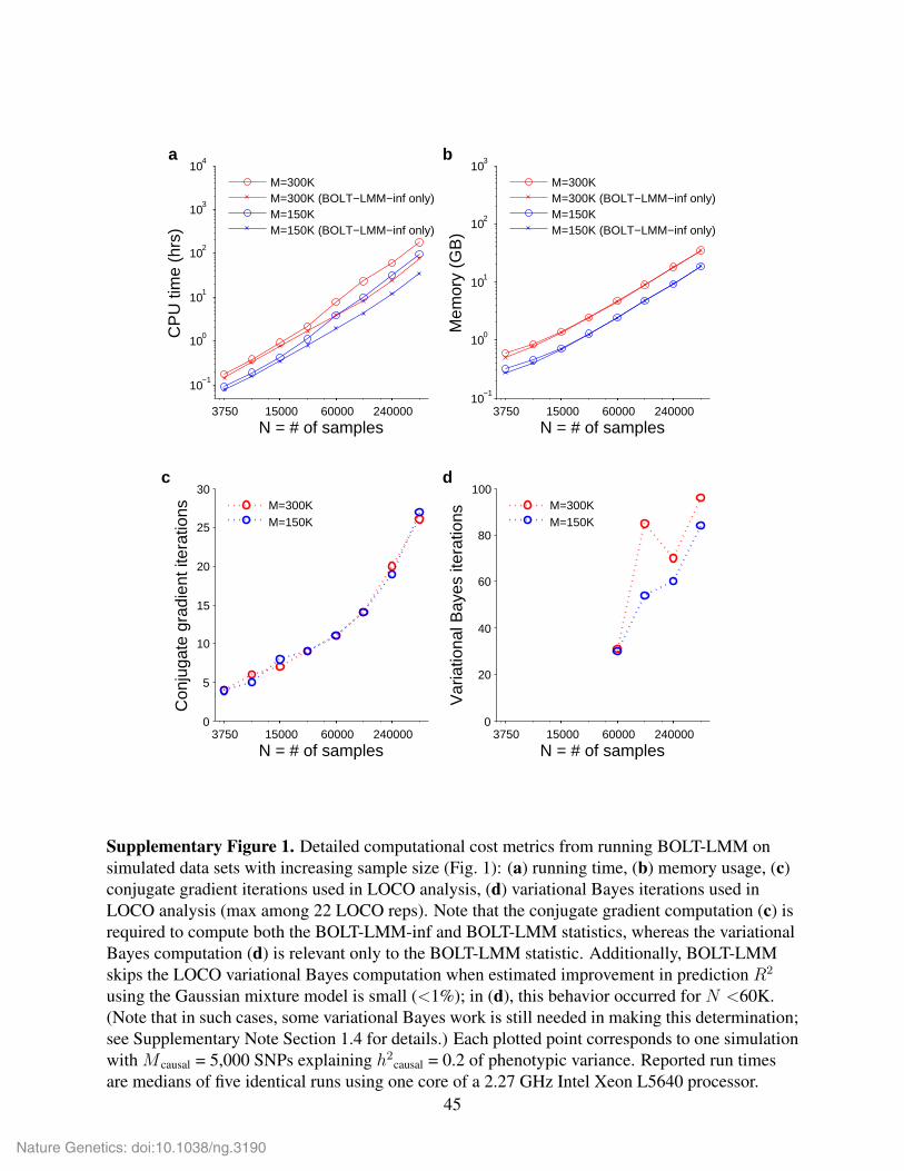
3750 15000 60000 240000
10−1
100
101
102
103
104
N = # of samples
CP
U ti
me
(hrs
)
a
M=300KM=300K (BOLT−LMM−inf only)M=150KM=150K (BOLT−LMM−inf only)
3750 15000 60000 24000010
−1
100
101
102
103
N = # of samples
Mem
ory
(GB
)
b
M=300KM=300K (BOLT−LMM−inf only)M=150KM=150K (BOLT−LMM−inf only)
3750 15000 60000 2400000
5
10
15
20
25
30
N = # of samples
Con
juga
te g
radi
ent i
tera
tions
c
M=300KM=150K
3750 15000 60000 2400000
20
40
60
80
100
N = # of samples
Var
iatio
nal B
ayes
iter
atio
ns
d
M=300KM=150K
Supplementary Figure 1. Detailed computational cost metrics from running BOLT-LMM onsimulated data sets with increasing sample size (Fig. 1): (a) running time, (b) memory usage, (c)conjugate gradient iterations used in LOCO analysis, (d) variational Bayes iterations used inLOCO analysis (max among 22 LOCO reps). Note that the conjugate gradient computation (c) isrequired to compute both the BOLT-LMM-inf and BOLT-LMM statistics, whereas the variationalBayes computation (d) is relevant only to the BOLT-LMM statistic. Additionally, BOLT-LMMskips the LOCO variational Bayes computation when estimated improvement in prediction R2
using the Gaussian mixture model is small (<1%); in (d), this behavior occurred for N <60K.(Note that in such cases, some variational Bayes work is still needed in making this determination;see Supplementary Note Section 1.4 for details.) Each plotted point corresponds to one simulationwith M causal = 5,000 SNPs explaining h2causal = 0.2 of phenotypic variance. Reported run timesare medians of five identical runs using one core of a 2.27 GHz Intel Xeon L5640 processor.
45
Nature Genetics: doi:10.1038/ng.3190

0.15 0.25 0.350
5
10
15
20
h2causal
CP
U ti
me
(hrs
)
2 ancestors per sample
a
N=60KN=30K
0.15 0.25 0.350
5
10
15
20
h2causal
Con
juga
te g
radi
ent i
tera
tions 2 ancestors per samplec
0.15 0.25 0.350
20
40
60
80
100
h2causal
Var
iatio
nal B
ayes
iter
atio
ns 2 ancestors per samplee
0.15 0.25 0.350
5
10
15
20
h2causal
CP
U ti
me
(hrs
)
10 ancestors per sampleb
0.15 0.25 0.350
5
10
15
20
h2causal
Con
juga
te g
radi
ent i
tera
tions 10 ancestors per sampled
0.15 0.25 0.350
20
40
60
80
100
h2causal
Var
iatio
nal B
ayes
iter
atio
ns 10 ancestors per samplef
Supplementary Figure 2. Dependence of BOLT-LMM computational cost metrics (seeSupplementary Fig. 1) on heritability explained by genotyped SNPs (h2g), sample size, and samplestructure. BOLT-LMM was run on simulated data sets with N = 30,000 or 60,000 samples, eachgenerated as a mosaic of genotype data from 2 (left panels) or 10 (right panels) random“ancestors” from the WTCCC2 data set (N = 15,633, M = 360K). Phenotypes were simulatedwith M causal = 5,000 SNPs explaining h2causal = 0.15–0.35 of phenotypic variance. In order tomeasure variational Bayes iterations (e, f) used in LOCO analysis for all parameter combinations,BOLT-LMM Gaussian mixture model analysis was run to completion even when estimatedimprovement in prediction R2 using the Gaussian mixture model was small (i.e., the defaultbehavior was overriden). Error bars, s.e.m., 10 simulations.
46
Nature Genetics: doi:10.1038/ng.3190

0 2500 5000 100000.3
0.4
0.5
0.6
0.7
0.8
0.9
1
Causal SNPs
Pow
er a
t sta
ndar
dize
d ef
fect
SN
Ps
α=0.05: BOLT−LMMα=0.05: BOLT−LMM−inf, GCTA−LOCOα=0.05: EMMAX, GEMMAα=0.01: BOLT−LMMα=0.01: BOLT−LMM−inf, GCTA−LOCOα=0.01: EMMAX, GEMMA
Supplementary Figure 3. Power of BOLT-LMM and existing mixed model association methodsto detect standardized effect SNPs in the simulations of Fig. 2 (real genotypes from the WTCCC2data set with N = 15,633 and M = 360K, simulated phenotypes with varying numbers of causalSNPs). Error bars, s.e.m., 100 simulations.
47
Nature Genetics: doi:10.1038/ng.3190

0 2500 5000 100005
5.5
6
6.5
7
7.5
8
8.5
9
9.5
10
Causal SNPs
Mea
n st
anda
rdiz
ed e
ffect
SN
P χ
2
a
BOLT−LMMBOLT−LMM−inf, GCTA−LOCOEMMAX, GEMMA
0 2500 5000 100000.8
0.85
0.9
0.95
1
1.05
1.1
1.15
Causal SNPs
Mea
n nu
ll S
NP
χ2
b
BOLT−LMMBOLT−LMM−inf, GCTA−LOCOEMMAX, GEMMA
Supplementary Figure 4. BOLT-LMM increases power to detect associations in simulationswhile maintaining false positive control. (a) Mean χ2 at standardized effect SNPs. (b) Mean χ2 atnull SNPs (i.e., SNPs not in LD with causal SNPs). Simulations used real genotypes from theWTCCC2 data set (N = 15,633, M = 360K) and simulated phenotypes with the specified numberof causal SNPs explaining 50% of phenotypic variance and 60 more standardized effect SNPsexplaining an additional 2% of the variance. Error bars, s.e.m., 100 simulations. Plotted data arefor BOLT-LMM, BOLT-LMM-inf, and EMMAX statistics. We verified on the first 5 simulationsthat the BOLT-LMM-inf and GCTA-LOCO statistics were nearly identical and that the EMMAXand GEMMA statistics were nearly identical (Supplementary Table 7).
48
Nature Genetics: doi:10.1038/ng.3190

250 2500 5000 10000 15000
1
1.05
1.1
1.15
1.2
1.25
1.3
1.35
1.4
1.45
Mcausal
= # of causal SNPsBO
LT−
LMM
χ2 /
LMM
χ2 a
t sta
ndar
dize
d S
NP
s
2 ancestors per sample
a
N=60K, h2g=0.355
N=60K, h2g=0.255
N=60K, h2g=0.155
N=30K, h2g=0.36
N=30K, h2g=0.26
N=30K, h2g=0.16
0 20 40 60 80 100
1
1.05
1.1
1.15
1.2
1.25
1.3
1.35
1.4
1.45
h2gN / M
causal
BO
LT−
LMM
χ2 /
LMM
χ2 a
t sta
ndar
dize
d S
NP
s
2 ancestors per samplec
250 2500 5000 10000 15000
1
1.05
1.1
1.15
1.2
1.25
1.3
1.35
1.4
1.45
Mcausal
= # of causal SNPsBO
LT−
LMM
χ2 /
LMM
χ2 a
t sta
ndar
dize
d S
NP
s
10 ancestors per sampleb
0 20 40 60 80 100
1
1.05
1.1
1.15
1.2
1.25
1.3
1.35
1.4
1.45
h2gN / M
causal
BO
LT−
LMM
χ2 /
LMM
χ2 a
t sta
ndar
dize
d S
NP
s10 ancestors per sampled
Supplementary Figure 5. Power increase of BOLT-LMM Gaussian mixture model associationanalysis over standard mixed model analysis as a function of sample size, number of causal SNPs,and heritability explained by genotyped SNPs (h2g). Plotted are ratios of mean χ2 BOLT-LMM vs.BOLT-LMM-inf statistics at standardized effect SNPs as a function of (a) M causal or (b)h2gN/M causal. This metric is equivalent to increase in effective sample size using the Gaussianmixture model. Data sets used N = 30,000 or 60,000 simulated individuals, each generated as amosaic of genotype data from 2 (left panels) or 10 (right panels) random “ancestors” from theWTCCC2 data set (N = 15,633, M = 360K). Phenotypes were simulated with M causal =2,500–15,000 SNPs explaining h2causal = 0.15–0.35 of phenotypic variance and 60 morestandardized effect SNPs explaining an additional 0.005 (N = 60K) or 0.01 (N = 30K) of thevariance. In all simulations, both BOLT-LMM and BOLT-LMM-inf statistics were properlycalibrated (mean χ2 = 1.00–1.01 at null SNPs). Error bars, s.e.m., 10 simulations.
49
Nature Genetics: doi:10.1038/ng.3190

0 10 20 30 400
10
20
30
40
χ2 expected
χ2 obs
erve
d: B
OLT
−LM
MNull SNPs
a
0 10 20 30 400
10
20
30
40
χ2 expected
χ2 obs
erve
d: B
OLT
−LM
M−
inf
Null SNPsb
0 10 20 30 400
10
20
30
40
χ2 expected
χ2 obs
erve
d: B
OLT
−LM
M
All SNPsc
0 10 20 30 400
10
20
30
40
χ2 expected
χ2 obs
erve
d: B
OLT
−LM
M−
inf
All SNPsd
Supplementary Figure 6. Q-Q plots of BOLT-LMM χ2 statistics (a, c) and BOLT-LMM-infχ2 statistics (b, d). The observed quantiles of both association statistics at null SNPs (a, b) matchtheoretical χ2 quantiles. The observed test statistics over all SNPs (c, d) show lift-off consistentwith polygenicity as simulated. Data shown are from one simulation using the setup of Fig. 2(real genotypes from the WTCCC2 data set with N = 15,633 and M = 360K, simulatedphenotypes with 5060 causal SNPs explaining 0.52 of phenotypic variance). To reduce clutter,5% of the SNPs are plotted.
50
Nature Genetics: doi:10.1038/ng.3190

0 5 10 15 20 25 30 350
5
10
15
20
25
30
35
BOLT−LMM−inf χ2
GC
TA
−LO
CO
χ2
Supplementary Figure 7. Scatter plot of BOLT-LMM-inf vs. GCTA-LOCO χ2 statistics.BOLT-LMM-inf and GCTA-LOCO are expected to differ slightly because GCTA-LOCO is thestandard prospective statistic whereas BOLT-LMM-inf is a retrospective statistic. Data shown arefrom one simulation using the setup of Fig. 2 (real genotypes from the WTCCC2 data set,simulated phenotypes with 5060 causal SNPs explaining 0.52 of phenotypic variance). To reduceclutter, 5% of the SNPs are plotted.
51
Nature Genetics: doi:10.1038/ng.3190

Supp
lem
enta
ryTa
ble
1.C
ompu
tatio
nalp
erfo
rman
ceof
mix
edm
odel
asso
ciat
ion
met
hods
NB
OLT
-LM
MB
OLT
-LM
M-i
nfG
CTA
-LO
CO
EM
MA
XG
EM
MA
FaST
-LM
MFa
ST-L
MM
-Sel
ect
3,75
00.
171
hr/0
.582
GB
0.14
1hr
/0.5
GB
1.15
hr/6
.31
GB
1.78
hr/3
.77
GB
3.28
hr/0
.323
GB
1.22
hr/2
5.4
GB
4.24
hr/2
5.5
GB
7,50
00.
385
hr/0
.847
GB
0.32
4hr
/0.7
71G
B5.
58hr
/15.
8G
B8.
79hr
/3.7
8G
B12
.2hr
/0.9
53G
B3.
34hr
/50.
9G
B15
.8hr
/54.
9G
B15
,000
0.91
hr/1
.39
GB
0.78
hr/1
.32
GB
31.4
hr/4
4.8
GB
32.1
hr/1
3.4
GB
50hr
/3.4
7G
BN
Aa
NA
a
30,0
002.
11hr
/2.4
5G
B1.
67hr
/2.4
1G
BN
Aa
129
hr/5
3.7
GB
NA
bN
Aa
NA
a
60,0
007.
93hr
/4.6
2G
B3.
94hr
/4.5
9G
BN
Aa
NA
aN
Ab
NA
aN
Aa
120,
000
23.4
hr/8
.96
GB
8.07
hr/8
.96
GB
NA
aN
Aa
NA
bN
Aa
NA
a
240,
000
60.8
hr/1
7.7
GB
24.1
hr/1
7.7
GB
NA
aN
Aa
NA
bN
Aa
NA
a
480,
000
177
hr/3
4.3
GB
76hr
/35.
1G
BN
Aa
NA
aN
Ab
NA
aN
Aa
Thi
sta
ble
prov
ides
the
num
eric
alda
ta(r
unni
ngtim
esan
dm
emor
ybe
nchm
arks
forv
ario
usm
ixed
mod
elm
etho
ds)p
lotte
din
Fig.
1as
wel
las
FaST
-LM
Mv2
.07
(usi
ngal
lmar
kers
).a M
etho
ddi
dno
tcom
plet
edu
eto
exce
edin
gth
e96
GB
ofm
emor
yav
aila
ble.
b Met
hod
did
notc
ompl
ete
due
toa
runt
ime
erro
r(se
gmen
tatio
nfa
ult)
.
52
Nature Genetics: doi:10.1038/ng.3190

Supplementary Table 2. BOLT-LMM increases power to detect associations in simulations
(a)
M causal PCA BOLT-LMM-inf BOLT-LMM1,250 6.55 (0.07) 6.92 (0.07) 8.71 (0.08)2,500 6.52 (0.07) 6.89 (0.08) 7.65 (0.09)5,000 6.56 (0.07) 6.94 (0.07) 7.23 (0.07)
10,000 6.56 (0.07) 6.94 (0.07) 7.04 (0.07)
(b)
h2causal PCA BOLT-LMM-inf BOLT-LMM0.3 6.41 (0.07) 6.54 (0.07) 6.71 (0.07)0.5 6.52 (0.07) 6.89 (0.08) 7.65 (0.09)0.7 6.63 (0.08) 7.39 (0.09) 9.71 (0.11)
(c)
N PCA BOLT-LMM-inf BOLT-LMM5,211 2.83 (0.04) 2.88 (0.04) 2.90 (0.04)
10,422 4.71 (0.06) 4.90 (0.06) 5.14 (0.06)15,633 6.52 (0.07) 6.89 (0.08) 7.65 (0.09)
These tables provide the numerical data (mean χ2 statistics at standardized effect SNPs) plotted inFig. 2.
53
Nature Genetics: doi:10.1038/ng.3190

Supplementary Table 3. Calibration of BOLT-LMM statistics in simulations with varyinggenetic architectures and sample sizes
(a)
M causal PCA BOLT-LMM-inf BOLT-LMM1,250 1.009 (0.001) 1.006 (0.001) 1.005 (0.001)2,500 1.008 (0.001) 1.005 (0.001) 1.004 (0.001)5,000 1.007 (0.001) 1.005 (0.001) 1.004 (0.001)
10,000 1.009 (0.001) 1.007 (0.001) 1.007 (0.001)
(b)
h2causal PCA BOLT-LMM-inf BOLT-LMM0.3 1.005 (0.001) 1.004 (0.001) 1.005 (0.001)0.5 1.008 (0.001) 1.005 (0.001) 1.004 (0.001)0.7 1.011 (0.001) 1.009 (0.001) 1.000 (0.001)
(c)
N PCA BOLT-LMM-inf BOLT-LMM5,211 1.002 (0.001) 1.004 (0.001) 1.004 (0.001)
10,422 1.005 (0.001) 1.005 (0.001) 1.005 (0.001)15,633 1.008 (0.001) 1.005 (0.001) 1.004 (0.001)
We report mean χ2 statistics at null SNPs in the simulations of Fig. 2. The very slight inflation ofBOLT-LMM and BOLT-LMM-inf arises from the use of approximate variance parameterestimates and from the fact that standard mixed model methods eliminate the effects ofstratification nearly perfectly but not completely (Supplementary Table 4).
54
Nature Genetics: doi:10.1038/ng.3190

Supplementary Table 4. Calibration of BOLT-LMM statistics using different variancecomponent estimation procedures
Variance component Leave-out h2strat = 0.01 h2strat = 0estimation procedure segments GCTA-LOCO BOLT-inf BOLT GCTA-LOCO BOLT-inf BOLTOnce with no left-out 22 NA 1.005 1.004 NA 1.004 1.002SNPs 100 NA 1.002 1.000 NA 1.001 0.999Independently for each 22 1.002 1.001 0.999 1.000 0.999 0.997leave-out segment 100 NA 1.000 0.998 NA 0.998 0.997
Mean GCTA-LOCO, BOLT-LMM-inf, and BOLT-LMM chi-squared statistics at null SNPscomputed using different methods for variance component analysis and different numbers ofleave-out segments. We used the same simulation setup as in Fig. 2 (real genotypes from theWTCCC2 data set, simulated phenotypes with 2560 causal SNPs explaining 0.52 of phenotypicvariance). We performed two sets of simulations: one with environmental stratification h2strat
explaining 0.01 of the variance, and the other with no environmental stratification. Thus, the topleft entries of 1.005 for BOLT-LMM-inf and 1.004 for BOLT-LMM correspond to the calibrationresults in Supplementary Table 3 for M causal = 2,500, h2causal = 0.5, N = 15,633 (appearing in eachof Supplementary Table 3a,b,c). Data shown are from 100 simulations, which gave a standarderror of 0.001 for all numbers above.By default, the BOLT-LMM algorithm estimates variance parameters once using all SNPs andthen reuses the variance estimates when computing association statistics, leaving each of the 22chromosomes out in turn. This procedure is an approximation of the theoretically precise methodof re-estimating variance parameters once per leave-out segment, which the BOLT-LMMsoftware offers as an alternative option (Online Methods). The quality of the approximation canalso be improved by subdividing chromosomes for leave-out analysis; we compare results with 22vs. 100 leave-out segments, which the BOLT-LMM software allows as well (Online Methods).GCTA-LOCO re-estimates variance components once for each of 22 left-out chromosomes.These simulations demonstrate that very slight (0.1–0.5%) inflation of χ2 test statistics can stemfrom two causes: (1) reusing the same variance parameter estimates across all LOCO reps ratherthan re-estimating them for each LOCO rep; and (2) near-complete but imperfect correction forstratification by mixed model methods [52]. The first source of slight inflation is specific to theBOLT-LMM approximation procedure but can be reduced by partitioning the genome into finerleave-out segments or eliminated by refitting variance parameters for each LOCO rep at a smallincrease in computational cost (Online Methods). This inflation does not increase with samplesize (Supplementary Table 3c). The second source of slight inflation is shared by all mixed modelmethods, as evidenced by the 0.2% inflation of GCTA-LOCO in the h2strat = 0.01 simulation, andscales with sample size and proportion of variance explained by ancestry in the same manner asinflation caused by genuine polygenic effects (see Supplementary Table 2 of ref. [12]). Tocompletely eliminate this source of very slight inflation, it is necessary to either include principalcomponents as fixed effects or include a second variance component that modelsancestry [12, 52–54]. However, we believe that this very slight inflation is not a significantproblem for standard mixed model methods or BOLT-LMM.
55
Nature Genetics: doi:10.1038/ng.3190

Supplementary Table 5. Type I error of BOLT-LMM and EMMAX association tests insimulations
Method α = 10−2 α = 10−4 α = 10−6 α = 5× 10⁻⁸
BOLT-LMM 1.02× 10⁻² 705103 1.04× 10⁻⁴ 7221 1.05× 10⁻⁶ 73 4× 10⁻⁸ 3BOLT-LMM-inf 1.02× 10⁻² 707636 1.03× 10⁻⁴ 7119 1.07× 10⁻⁶ 74 6× 10⁻⁸ 4EMMAX 0.63× 10⁻² 434081 0.39× 10⁻⁴ 2673 0.32× 10⁻⁶ 22 0× 10−8 0
Type I error rates and counts for test statistics at null SNPs in the simulations of Fig. 2 (realgenotypes from the WTCCC2 data set, simulated phenotypes with causal SNPs explaining 52%of phenotypic variance and environmental stratification explaining 1% of phenotypic variance).To increase statistical resolution, we combined data from all 400 simulations (with 1310, 2560,5060, and 10060 causal SNPs, 100 simulations each) for a total of 69,293,600 hypothesis tests.Type I error was statistically indistinguishable between different subsets of 100 simulations. Thevery slight upward bias of actual vs. expected Type I error rates for the BOLT-LMM-inf andBOLT-LMM association tests is explained by very slight (0.1–0.5%) inflation of χ2 test statistics(Supplementary Table 4), which can be mitigated by performing a more precise varianceparameter calculation if desired (Online Methods).
56
Nature Genetics: doi:10.1038/ng.3190

Supplementary Table 6. Power and calibration of BOLT-LMM statistics, BOLT-LMM withMCMC, and FaST-LMM-Select in simulations
(a) M causal = 1,250
Method Mean χ2 at Mean χ2 at LD Scorestd. effect SNPs null SNPs intercept
PCA 2.843 (0.041) 1.003 (0.001) 1.008 (0.001)BOLT-LMM-inf 2.923 (0.041) 1.005 (0.001) 1.008 (0.001)BOLT-LMM 3.174 (0.045) 1.003 (0.001) 1.008 (0.001)BOLT-LMM with MCMC 3.154 (0.045) 1.004 (0.001) 1.008 (0.001)FaST-LMM-Select 2.852 (0.037) 1.021 (0.003) 1.026 (0.002)
(b) M causal = 500
Method Mean χ2 at Mean χ2 at LD Scorestd. effect SNPs null SNPs intercept
PCA 2.918 (0.045) 1.004 (0.001) 1.010 (0.001)BOLT-LMM-inf 2.988 (0.047) 1.005 (0.001) 1.010 (0.001)BOLT-LMM 4.181 (0.064) 1.002 (0.001) 1.010 (0.001)FaST-LMM-Select 3.520 (0.044) 1.017 (0.002) 1.021 (0.002)
We report mean χ2 statistics at standardized effect SNPs, mean χ2 statistics at null SNPs, and LDScore intercepts [24] of association statistics computed by linear regression with PC covariates(PCA), variants of BOLT-LMM, and FaST-LMM-Select over 100 simulations. Each simulationused real genotypes from N = 5,211 WTCCC2 samples and simulated phenotypes with (a) 1,250or (b) 500 causal SNPs explaining 70% of variance, 60 standardized effect SNPs explaining 2%of variance, and a 1% ancestry effect. In simulation group (a), we ran the MCMC modification ofBOLT-LMM for 1,000 iterations of the Gibbs sampler through all SNPs. We do not reportMCMC results for (b) because the Gibbs sampler had not converged after 1,000 iterations; wehypothesize the MCMC was slow to mix in this case because of the small number of causal SNPsresulting in a highly nonlinear model involving a few large effect sizes.In simulation group (a) with M causal = 1,250, FaST-LMM-Select typically selected 100 top SNPsto include in the mixed model; in (b) with Mcausal = 500, FaST-LMM-Select typically selected 300top SNPs. In (a), we observed that FaST-LMM achieved lower power than BOLT-LMM-inf (asmeasured by mean χ2 at standardized effect SNPs), which we found surprising, especially giventhat FaST-LMM-Select reported that including 100 top SNPs in the mixed model achieved a 7%average reduction in cross-validation prediction MSE (which is in between that achieved byBOLT-LMM-inf and BOLT-LMM, consistent with our expectations). We are unsure why thisimprovement in out-of-sample prediction MSE did not translate into improved association power,although we also noticed that in (b), the association power achieved by FaST-LMM-Select waslower than we expected given its cross-validation report (≈30% reduction in MSE).The calibration results (mean χ2 at null SNPs) also show that in these simulations, the choice ofFaST-LMM-Select to use ≈100–300 SNPs in the mixed model led to mild inflation due toinadequate stratification correction. Accordingly, the LD Score intercept for FaST-LMM-Select isinflated relative to the other methods. (Note that the LD Score intercepts for the other methods,which are properly calibrated, are slightly greater than 1 due to attenuation bias; seeSupplementary Note Section 1.5 for a detailed discussion.) Normalizing FaST-LMM-Select tohave the same LD Score intercept as BOLT-LMM-inf (which is how BOLT-LMM is calibrated)produces a properly calibrated statistic: e.g., in (a) we get 1.021 / (1.026/1.008) = 1.003, which issimilar to the other methods. Note, however, that calibration alone does not solve the problem ofpotential false positives at unusually differentiated markers.57
Nature Genetics: doi:10.1038/ng.3190

Supplementary Table 7. Correlations between mixed model statistics computed by variousmixed model methods under the infinitesimal model
R2 (s.e.m.) GCTA-LOCO GEMMABOLT-LMM-inf 0.999471 (0.000017) 0.962928 (0.000916)EMMAX 0.963326 (0.000969) 0.999997 (0.000000)
Squared correlation coefficients between χ2 association statistics over all SNPs computed byvarious mixed model methods using the simulation setup of Fig. 2 (real genotypes from theWTCCC2 data set, simulated phenotypes with 5060 causal SNPs explaining 0.52 of phenotypicvariance). Means and standard errors over 5 simulations are reported. BOLT-LMM-inf andGCTA-LOCO statistics both avoid proximal contamination via LOCO analysis but are expectedto differ slightly because GCTA-LOCO is the standard prospective statistic whereasBOLT-LMM-inf is a retrospective statistic. EMMAX and GEMMA are both susceptible toproximal contamination but are expected to differ slightly because GEMMA is an exact statisticwhereas EMMAX is an approximate statistic.
58
Nature Genetics: doi:10.1038/ng.3190

Supplementary Table 8. Comparison of χ2 statistics computed by various methods atknown SNPs for WGHS phenotypes
# known # tagged # p < 0.05 Mean log fold # p < 0.05 Mean log foldPhenotype SNPs SNPs PCA & LMM χ2 LMM / PCA PCA & BOLT χ2 BOLT / PCAApoB 59 (ref. [55]) 57 40 2.3 (1.4) 40 9.9 (2.1)LDL 59 (ref. [55]) 57 45 1.4 (1.1) 45 8.7 (1.7)HDL 72 (ref. [55]) 72 55 3.4 (1.2) 55 9.4 (1.8)Cholesterol 73 (ref. [55]) 71 53 1.8 (1.1) 54 5.5 (1.2)Triglycerides 41 (ref. [55]) 39 29 -0.6 (1.8) 29 1.7 (2.0)Height 180 (ref. [56]) 170 131 6.0 (1.5) 134 6.2 (1.6)BMI 32 (ref. [57]) 31 18 4.2 (1.8) 18 3.8 (1.8)SystolicBP 20 (ref. [58]) 20 11 2.6 (1.9) 11 2.6 (1.9)DiastolicBP 19 (ref. [58]) 19 9 3.2 (1.8) 9 3.0 (2.0)
The first two data columns provide additional information about known SNPs used in the powercomparison of Supplementary Table 9: # known SNPs, number of genome-wide significantassociated SNPs reported in largest GWAS to date; # tagged SNPs, number of such SNPs with anR2 ≥ 0.2 tagging SNP typed in WGHS. (Note that for the ApoB phenotype, we used knownSNPs for the closely related LDL phenotype.) Sums of χ2 statistics compared in SupplementaryTable 9 were computed across the WGHS-typed tagging SNPs.We also report here one additional metric for increase of power: Mean log fold-change inχ2 statistics at tagging SNPs. This metric weights all tagging SNPs evenly (SupplementaryTable 9), whereas comparing sums of χ2 statistics weights stronger associations more heavily.Because log fold-change is sensitive to noise from non-replicating SNPs, we restrict to taggingSNPs with at least nominal significance (p < 0.05) according to both methods being compared.Methods: PCA, linear regression using 10 principal components as covariates; LMM,BOLT-LMM-inf; BOLT, BOLT-LMM. Errors, s.e.m.
59
Nature Genetics: doi:10.1038/ng.3190
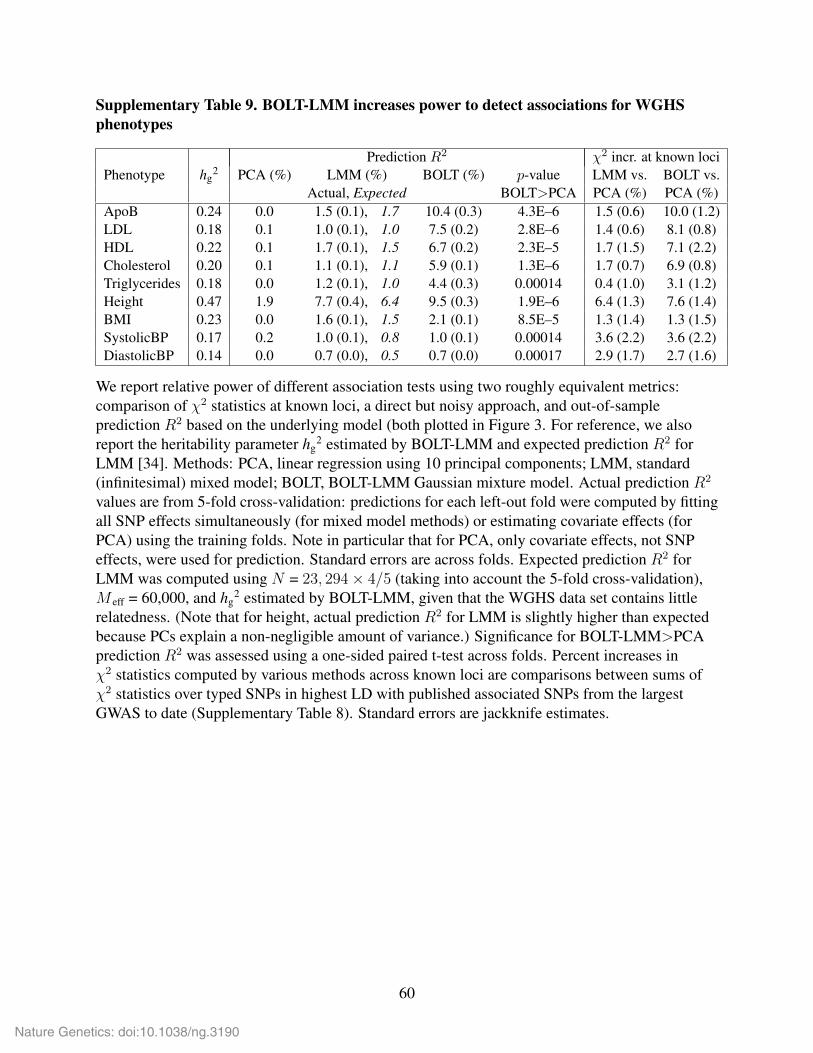
Supplementary Table 9. BOLT-LMM increases power to detect associations for WGHSphenotypes
Prediction R2 χ2 incr. at known lociPhenotype hg
2 PCA (%) LMM (%) BOLT (%) p-value LMM vs. BOLT vs.Actual, Expected BOLT>PCA PCA (%) PCA (%)
ApoB 0.24 0.0 1.5 (0.1), 1.7 10.4 (0.3) 4.3E–6 1.5 (0.6) 10.0 (1.2)LDL 0.18 0.1 1.0 (0.1), 1.0 7.5 (0.2) 2.8E–6 1.4 (0.6) 8.1 (0.8)HDL 0.22 0.1 1.7 (0.1), 1.5 6.7 (0.2) 2.3E–5 1.7 (1.5) 7.1 (2.2)Cholesterol 0.20 0.1 1.1 (0.1), 1.1 5.9 (0.1) 1.3E–6 1.7 (0.7) 6.9 (0.8)Triglycerides 0.18 0.0 1.2 (0.1), 1.0 4.4 (0.3) 0.00014 0.4 (1.0) 3.1 (1.2)Height 0.47 1.9 7.7 (0.4), 6.4 9.5 (0.3) 1.9E–6 6.4 (1.3) 7.6 (1.4)BMI 0.23 0.0 1.6 (0.1), 1.5 2.1 (0.1) 8.5E–5 1.3 (1.4) 1.3 (1.5)SystolicBP 0.17 0.2 1.0 (0.1), 0.8 1.0 (0.1) 0.00014 3.6 (2.2) 3.6 (2.2)DiastolicBP 0.14 0.0 0.7 (0.0), 0.5 0.7 (0.0) 0.00017 2.9 (1.7) 2.7 (1.6)
We report relative power of different association tests using two roughly equivalent metrics:comparison of χ2 statistics at known loci, a direct but noisy approach, and out-of-sampleprediction R2 based on the underlying model (both plotted in Figure 3. For reference, we alsoreport the heritability parameter hg
2 estimated by BOLT-LMM and expected prediction R2 forLMM [34]. Methods: PCA, linear regression using 10 principal components; LMM, standard(infinitesimal) mixed model; BOLT, BOLT-LMM Gaussian mixture model. Actual prediction R2
values are from 5-fold cross-validation: predictions for each left-out fold were computed by fittingall SNP effects simultaneously (for mixed model methods) or estimating covariate effects (forPCA) using the training folds. Note in particular that for PCA, only covariate effects, not SNPeffects, were used for prediction. Standard errors are across folds. Expected prediction R2 forLMM was computed using N = 23, 294× 4/5 (taking into account the 5-fold cross-validation),M eff = 60,000, and hg
2 estimated by BOLT-LMM, given that the WGHS data set contains littlerelatedness. (Note that for height, actual prediction R2 for LMM is slightly higher than expectedbecause PCs explain a non-negligible amount of variance.) Significance for BOLT-LMM>PCAprediction R2 was assessed using a one-sided paired t-test across folds. Percent increases inχ2 statistics computed by various methods across known loci are comparisons between sums ofχ2 statistics over typed SNPs in highest LD with published associated SNPs from the largestGWAS to date (Supplementary Table 8). Standard errors are jackknife estimates.
60
Nature Genetics: doi:10.1038/ng.3190

Supplementary Table 10. Effect size mixture parameters chosen by BOLT-LMM for WGHSphenotypes
Phenotype hg2 f2 p
ApoB 0.24 0.1 0.01LDL 0.18 0.1 0.01HDL 0.22 0.1 0.01Cholesterol 0.20 0.1 0.01Triglycerides 0.18 0.1 0.01Height 0.47 0.3 0.02BMI 0.23 0.5 0.01SystolicBP 0.17 0.5 0.5DiastolicBP 0.14 0.5 0.01
We report the best-fit mixture-of-Gaussians prior on SNP effect sizes determined by BOLT-LMMusing cross-validation to optimize out-of-sample prediction R2. The spike and slab mixture ofGaussians is parameterized by the total variance attributed to the combined Gaussian mixturealong with two mixture parameters: f2, the proportion of variance allotted to the spike component(small-effect SNPs), and p, the probability that a SNP effect is drawn from the slab component(large-effect SNPs). Note that f2 = 0.5, p = 0.5 corresponds to the infinitesimal model: whenf2 = 1− p, the two Gaussians are identical and the mixture is degenerate.
61
Nature Genetics: doi:10.1038/ng.3190
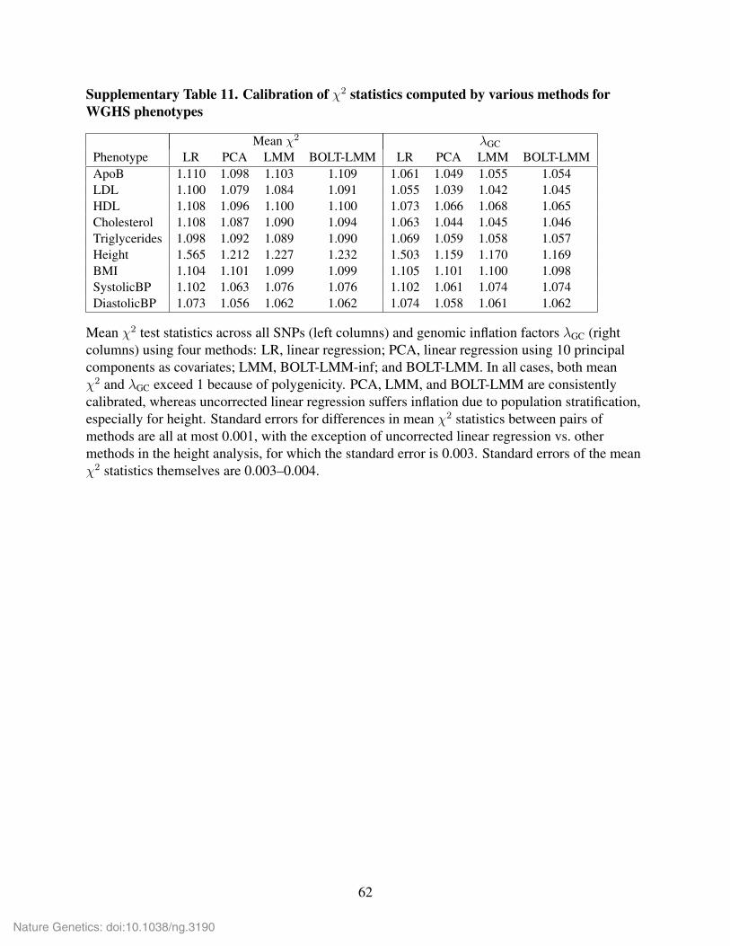
Supplementary Table 11. Calibration of χ2 statistics computed by various methods forWGHS phenotypes
Mean χ2 λGCPhenotype LR PCA LMM BOLT-LMM LR PCA LMM BOLT-LMMApoB 1.110 1.098 1.103 1.109 1.061 1.049 1.055 1.054LDL 1.100 1.079 1.084 1.091 1.055 1.039 1.042 1.045HDL 1.108 1.096 1.100 1.100 1.073 1.066 1.068 1.065Cholesterol 1.108 1.087 1.090 1.094 1.063 1.044 1.045 1.046Triglycerides 1.098 1.092 1.089 1.090 1.069 1.059 1.058 1.057Height 1.565 1.212 1.227 1.232 1.503 1.159 1.170 1.169BMI 1.104 1.101 1.099 1.099 1.105 1.101 1.100 1.098SystolicBP 1.102 1.063 1.076 1.076 1.102 1.061 1.074 1.074DiastolicBP 1.073 1.056 1.062 1.062 1.074 1.058 1.061 1.062
Mean χ2 test statistics across all SNPs (left columns) and genomic inflation factors λGC (rightcolumns) using four methods: LR, linear regression; PCA, linear regression using 10 principalcomponents as covariates; LMM, BOLT-LMM-inf; and BOLT-LMM. In all cases, both meanχ2 and λGC exceed 1 because of polygenicity. PCA, LMM, and BOLT-LMM are consistentlycalibrated, whereas uncorrected linear regression suffers inflation due to population stratification,especially for height. Standard errors for differences in mean χ2 statistics between pairs ofmethods are all at most 0.001, with the exception of uncorrected linear regression vs. othermethods in the height analysis, for which the standard error is 0.003. Standard errors of the meanχ2 statistics themselves are 0.003–0.004.
62
Nature Genetics: doi:10.1038/ng.3190

Supplementary Table 12. Control for stratification: Height p-values at lactase computed byvarious methods
LR PCA LMM BOLT-LMMχ2 statistic 33.09 3.66 6.56 6.07p-value 9× 10⁻⁹ 0.06 0.01 0.01
We report χ2 statistics and p-values computed at rs2011946, the SNP typed in WGHS withhighest LD (R2 = 0.64 in 1000 Genomes reference samples) to lactase-associated SNPrs4988235. Methods: LR, linear regression; PCA, linear regression using 10 principalcomponents as covariates; LMM, BOLT-LMM-inf; and default BOLT-LMM.
63
Nature Genetics: doi:10.1038/ng.3190

Supplementary Table 13. Power of mixed model association vs. linear regression forsimulated case-control ascertained traits
(a) h2g = 0.25 (for liabilities underlying case-control phenotype)Case prevalence
Method 50% 10% 5% 1% 0.1%Linear regression 2.828 (0.010) 3.723 (0.015) 4.401 (0.015) 6.206 (0.020) 9.179 (0.026)BOLT-LMM-inf 2.862 (0.010) 3.739 (0.015) 4.384 (0.015) 5.965 (0.018) 8.212 (0.023)BOLT-LMM 2.887 (0.011) 3.767 (0.015) 4.397 (0.014) 5.859 (0.022) 7.869 (0.025)
(b) h2g = 0.5 (for liabilities underlying case-control phenotype)Case prevalence
Method 50% 10% 5% 1% 0.1%Linear regression 4.661 (0.014) 6.452 (0.021) 7.756 (0.023) 11.360 (0.030) 17.290 (0.043)BOLT-LMM-inf 4.904 (0.016) 6.582 (0.022) 7.662 (0.021) 10.202 (0.025) 13.252 (0.033)BOLT-LMM 5.165 (0.018) 6.798 (0.026) 7.826 (0.024) 9.816 (0.034) 12.326 (0.037)
We compare mean χ2 statistics over causal SNPs for linear regression, BOLT-LMM-inf, andBOLT-LMM analysis of simulated case-control traits with prevalences ranging from 50%–0.1%.We simulated genotypes by generating individuals as mosaics of up to 100 random “ancestors”from the WTCCC2 data set, resampling ancestors every 500 SNPs. We restricted the SNP set tothe first 2,500 SNPs on each autosome, for a total of M = 55,000 SNPs (so that M effective ≈10,000 independent SNPs). We simulated case-control phenotypes using a liability thresholdmodel in which we first generated continuous phenotypes with (a) h2g = 0.25 or (b) h2g = 0.5explained by M causal = 1,000 markers and then defined cases as individuals with phenotypesexceeding a threshold corresponding to the desired prevalence. In each simulation, we ascertained5,000 cases and 5,000 controls for a total of N = 10,000 simulated individuals. We then ranassociation analysis on the ascertained samples. Errors, s.e.m. over 100 simulations.The results show that for non-ascertained traits, power of linear regression < BOLT-LMM-inf <BOLT-LMM, consistent with our findings for quantitative traits. This trend reverses forascertained traits at a prevalence near 5%. For the infinitesimal mixed model vs. linear regression,this result is consistent with the findings of ref. [12], which also observes that the relativereduction in test statistics increases with h2g and the ratio N / M effective in addition to ascertainmentseverity. In our simulations, N ≈M effective, so these simulations correspond to N ≈ 60,000 in realdata sets, which have M effective ≈ 60,000 [12]. For data sets with fewer than 60,000 samples,case-control ascertainment will present less of a problem for mixed model methods than indicatedabove.
64
Nature Genetics: doi:10.1038/ng.3190

Supplementary Table 14. Precision of infinitesimal mixed model statistic calibration
Phenotype Mean prospective stat Mean retrospective stat Calibration factorat 30 random SNPs (pre-calib.) at same SNPs cinf, equation (9)
ApoB 1.285 1.281 0.996 (0.001)LDL 1.013 1.011 0.998 (0.000)HDL 1.026 1.024 0.997 (0.001)Cholesterol 0.989 0.986 0.997 (0.000)Triglycerides 0.881 0.879 0.998 (0.000)Height 0.783 0.777 0.993 (0.001)BMI 0.900 0.897 0.997 (0.001)Systolic BP 0.853 0.849 0.996 (0.001)Diastolic BP 0.770 0.769 0.998 (0.001)
We report the BOLT-LMM-inf calibration factor for the nine analyzed WGHS phenotypes. Thiscalibration is similar to GRAMMAR-Gamma [10] but is estimated by computing statistics at only30 SNPs. The standard errors (jackknife estimates) show that 30 SNPs are enough to achieve highcalibration precision.
65
Nature Genetics: doi:10.1038/ng.3190

Supplementary Table 15. LD Score calibration factors in BOLT-LMM analyses of WGHSphenotypes
Phenotype Calibration factor c, equation (11)ApoB 1.004 (0.003)LDL 1.001 (0.002)HDL 1.001 (0.002)Cholesterol 0.999 (0.002)Triglycerides 1.000 (0.001)Height 0.997 (0.001)BMI 0.998 (0.001)Systolic BP 0.996 (0.000)Diastolic BP 0.998 (0.000)
We report the BOLT-LMM calibration factor for the nine analyzed WGHS phenotypes, whichequals the ratio of the LD Score intercepts of the uncalibrated BOLT-LMM statistic to that of theBOLT-LMM-inf statistic. Standard errors are jackknife estimates leaving out each chromosome inturn.
66
Nature Genetics: doi:10.1038/ng.3190