superstructured fiber bragg gratings in · 2017-01-31 · technique for their fabrication by meltz...

SUPERSTRUCTURED FIBER BRAGG GRATINGS AND APPLICATIONS

IN MICROWAVE SIGNAL PROCESSING

Sebastien Blais

Thesis submitted to the

Faculty of Graduate and Postdoctoral Studies

in partial fulfillment of the requirements

for the Doctorate in Philosophy degree in Electrical and Computer Engineering

Ottawa-Carleton Institute of Electrical and Computer Engineering

School of Electrical Engineering and Computer Science

Faculty of Engineering

University Of Ottawa

© Sebastien Blais, Ottawa, Canada, 2014

ABSTRACT

Since their discovery in 1978 by Hill et al. and the development of the transverse holographic

technique for their fabrication by Meltz et al. in 1989, fiber Bragg gratings (FBG) have

become an important device for applications in optical communications, optical signal

processing and fiber-optical sensors.

A superstructured fiber Bragg grating (SFBG), also called a sampled fiber Bragg grating, is a

special FBG that consists of a several small FBGs placed in close proximity to one another.

SFBGs have attracted much attention in recent years with the discovery of techniques

allowing the creation of equivalent chirp or equivalent phase shifts. The biggest advantage of

an SFBG with equivalent chirp or equivalent phase shifts is the possibility to design and

fabricate gratings with greatly varying phase and amplitude responses by adjusting the spatial

profile of the superstructure. The realization of SFBGs with equivalent chirp or equivalent

phase shifts requires only sub-millimeter precision. This is a relief from the sub-micron

precision required by traditional approaches.

In this thesis, the mathematical modeling of FBGs and SFBGs is reviewed. The use of

SFBGs for various applications in photonic microwave signal processing is considered.

Four main topics are presented in this thesis. The first topic is the use of SFBG as a photonic

true-time delay (TTD) beamformer for phased array antennas (PAAs).

The second topic addresses non-linearities in the group delay response of an SFBG with

equivalent chirp in its sampling period. An SFBG with an equivalent chirp using only a linear

- ii -

chirp coefficient may yield a group delay response that deviates from the linear response

required by a TTD beamformer. In the thesis, a technique to improve the linearity of the

group delay response is proposed and an adaptive algorithm to find the optimal linear and

non-linear chirp coefficients to produce the best linear group delay response is described.

Since no closed-form solution exists to represent the amplitude and phase responses of an

SFBG, we rely on a Fourier transform analogy under a weak grating approximation as a

starting point in the design of an SFBG. Simulations are then used to refine the response of

the SFBG. The algorithm proposed provides an optimal set of chirp coefficients that

minimizes the error in the group delay response. Four gratings are fabricated using the

optimized chirp coefficients and their application in a TTD PAA system is discussed.

The third topic discusses the use of an SFBG with equivalent phase shifts in its sampling

period as a means to realize optical single sideband (SSB) modulation. SSB modulation

eliminates the power penalty caused by chromatic dispersion experienced by an optical signal

traveling through a long length of optical fiber. By introducing two π phase shifts through

equivalent sampling to the SFBG, two ultra-narrow transmission bands are created in the

grating stop band of the +/- 1st spectral orders. In the proposed system, a double-sideband

plus carrier (DSB+C) modulated optical signal is sent to the input of an optical SSB filter

based on the equivalent phase-shift SFBG in order to select the optical carrier and a single

sideband, effectively blocking one sideband from propagating.

Finally, the fourth topic focuses on the implementation of a photonic microwave bandpass

filter based on an SFBG with equivalent chirp. Photonic microwave filters are used to

process microwave signals in the optical domain. By using a technique called phase-

modulation to intensity-modulation (PM-IM) conversion, a two-tap delay line filter is created

- iii -

with one negative tap. A single SFBG with a chirp in its sampling period is used as a means

to achieve the PM-IM conversion for the two taps. Two phase modulated optical carriers are

used to generate the two taps, each entering a different port of the SFBG and thus

experiencing an opposite dispersion value. The two optical signals are then recombined

before being sent to a photodetector (PD) where the filtered microwave signal is recovered.

- iv -

ACKNOWLEDGEMENTS

Foremost, I would like to express my sincere gratitude to my advisor, Prof. Jianping Yao, for

the continuous support of my Ph.D. study and research, for his patience, motivation,

enthusiasm, and immense knowledge. Dr. Yao's guidance helped me focus my research on

relevant topics in the area of microwave photonics. His critical eye was of inconsiderable

value for the publication of our research results and for the writing of this thesis.

I would also like to thank the members of my thesis committee: Prof. Jacques Albert and

Prof. Tet Hin Yeap, as well as my colleagues at the Microwave Photonics Research

Laboratory at the University of Ottawa.

Last but not the least; I would like to thank my family: my parents Michel and Louise, for

inspiring me and supporting me throughout my life and my wife, Karine, for her caring and

supporting role throughout this endeavor.

- v -

TABLE OF CONTENTS

Abstract ...................................................................................................................................... i

Acknowledgements .................................................................................................................. iv

Table of Contents ...................................................................................................................... v

List of Figures ........................................................................................................................ viii

List of Tables .......................................................................................................................... xv

List of Acronyms ................................................................................................................... xvi

List of Publications ................................................................................................................ xix

CHAPTER 1 Introduction ......................................................................................................... 1

1.1 Background review .................................................................................................... 1

1.2 Major contributions of this thesis ............................................................................... 7

1.3 Organization of this thesis ........................................................................................ 10

CHAPTER 2 Theoretical Overview........................................................................................ 12

2.1 Fiber Bragg Gratings ................................................................................................ 12

2.1.1 Mathematical model of Bragg gratings............................................................. 13

2.1.2 Photosensitivity ................................................................................................. 27

2.1.3 Fabrication of Bragg gratings ........................................................................... 28

2.2 Superstructured Fiber Bragg Gratings...................................................................... 31

2.2.1 Uniform Superstructured Fiber Bragg Gratings ............................................... 31

2.2.2 Equivalent Phase-Shifted Superstructured Fiber Bragg Gratings ..................... 50

2.2.3 Equivalent Chirp in Superstructured Fiber Bragg Gratings .............................. 53

2.3 Phased Array Antennas ............................................................................................ 55

2.3.1 Two-elements array .......................................................................................... 55

- vi -

2.3.2 N-element linear array ...................................................................................... 58

2.3.3 Planar array ....................................................................................................... 59

2.3.4 Far-field radiation pattern ................................................................................. 61

2.3.5 True time delay ................................................................................................. 65

2.3.6 Photonic true time delay ................................................................................... 71

CHAPTER 3 Photonic True-Time Delay Beamforming Based on Superstructured Fiber

Bragg Gratings With Linearly Increasing Equivalent Chirps ................................................. 73

3.1 SFBG with equivalent chirp in their sampling periods for use in TTD applications 74

3.2 Experimental results ................................................................................................. 84

3.3 Summary .................................................................................................................. 87

CHAPTER 4 Linearization of the Group Delay Response of Equivalent-Chirped

Superstructured Fiber Bragg Gratings .................................................................................... 89

4.1 Simulation study of the linearization of the group delay response of equivalent-

chirped SFBG ...................................................................................................................... 89

4.2 Simulation algorithms to linearize the group delay response of SFBG ................... 94

4.3 Fabrication of linearized equivalent-chirped SFBG............................................... 108

4.4 Error analysis of the designed and fabricated SFBGs ............................................ 120

4.4.1 Simulated and experimental grating responses ............................................... 121

4.5 Summary ................................................................................................................ 135

CHAPTER 5 Optical Single Sideband Modulation using an Ultra-Narrow Dual-

Transmission-Band Fiber Bragg Grating .............................................................................. 136

5.1 SSB modulator based on equivalent phase shift in SFBG ..................................... 137

5.2 Experimental results ............................................................................................... 139

5.3 Evaluation of dispersion effects on the recovered electrical signal ....................... 144

5.3.1 Double sideband modulation .......................................................................... 144

5.3.2 Single sideband modulation ............................................................................ 149

5.3.3 Dispersion effects of a single mode fiber ....................................................... 150

- vii -

5.3.4 Photodetector .................................................................................................. 151

5.3.5 Recovered microwave signal by a photodetector ........................................... 154

5.3.6 Impact on system performance ....................................................................... 156

5.4 Summary ................................................................................................................ 157

CHAPTER 6 All-Optical Bandpass Microwave Filter Based on a Superstructured Fiber

Bragg Grating with Equivalent Chirp ................................................................................... 159

6.1 All-optical bandpass microwave filter ................................................................... 159

6.2 PM-IM conversion ................................................................................................. 160

6.3 All-optical bandpass microwave filter configuration ............................................. 162

6.4 Summary ................................................................................................................ 168

CHAPTER 7 Conclusion and Future Work .......................................................................... 170

7.1 Conclusions ............................................................................................................ 170

7.2 Future work ............................................................................................................ 172

Bibliography ......................................................................................................................... 173

Appendix I Source code for the linearization of the group delay response in SFBGs with an

equivalent linear chirp in their sampling period ................................................................... 187

- viii -

LIST OF FIGURES

Fig. 1. Simulation results of the (a) reflection spectrum and (b) delay induced by a 4-mm long Bragg

grating with an “ac” index change of 210-4. ............................................................................... 16

Fig. 2. Refractive index modulation amplitude of (a) a uniform Bragg grating, (b) a Gaussian-

apodized Bragg grating with simple refractive index modulation amplitude change and (c) a

Gaussian-apodized Bragg grating with a constant average refractive index with a modulation

depth of 0.0002. ............................................................................................................................ 19

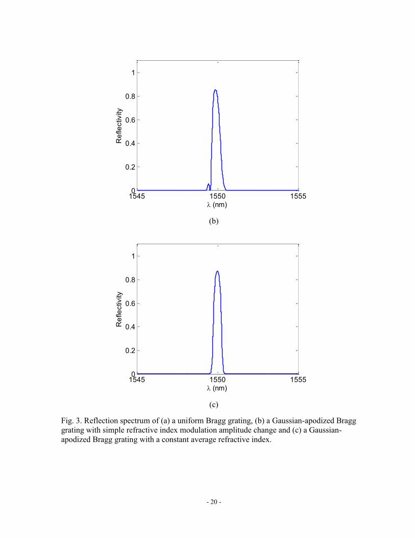
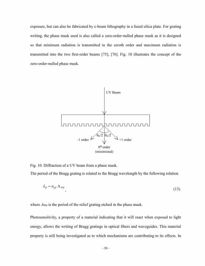
Fig. 3. Reflection spectrum of (a) a uniform Bragg grating, (b) a Gaussian-apodized Bragg grating

with simple refractive index modulation amplitude change and (c) a Gaussian-apodized Bragg

grating with a constant average refractive index. ......................................................................... 20

Fig. 4. Group delay of (a) a uniform Bragg grating, (b) a Gaussian-apodized Bragg grating with

simple refractive index modulation amplitude change and (c) a Gaussian-apodized Bragg grating

with a constant average refractive index. ..................................................................................... 22

Fig. 5. Diagram representing the transfer matrix method principle for a uniform grating. .................. 23

Fig. 6. Diagram showing the principle of the transfer matrix method for a non-uniform grating. ....... 24

Fig. 7. Simulation results of the (a) reflection response and (b) delay induced by a 10-mm long

chirped Bragg grating with a Bragg wavelength chirp of 9 nm. The refractive index modulation

is equal to 10-4. ............................................................................................................................. 26

Fig. 8. Simulation results of the (a) reflection response and (b) delay induced by a 10-mm long

Gaussian-apodized Bragg grating with a Bragg wavelength chirp of 9 nm. The refractive index

modulation is equal to 10-4. .......................................................................................................... 27

Fig. 9. Holographic method to write Bragg gratings. ........................................................................... 29

Fig. 10. Diffraction of a UV beam from a phase mask. ....................................................................... 30

Fig. 11. Refractive index profile of a superstructured fiber Bragg grating made of N sections. .......... 32

Fig. 12. Amplitude response (a), group delay response (b) and refractive index profile (c) of a

uniformly sampled SFBG, with Z0 = 0.68 mm, Ls = 0.36 mm and N = 40. The blue rectangles of

the refractive index profile are in fact sinusoidal with a very small period.................................. 34

Fig. 13. Spatial (a) and spectral (b) relationship in a superstructured fiber Bragg grating with uniform

sampling period and uniform apodization. ................................................................................... 36

Fig. 14. Effect of the sampling period, Z0, on the spectrum of an SFBG. For all SFBGs, Ls = 0.36 mm,

N = 40. For (a) and (b), Z0 = 0.50 mm; for (c) and (d), Z0 = 1.25 mm; for (e) and (f), Z0 = 2.00

- ix -

mm. (a), (c) and (e) show the amplitude response of the SFBG; (b), (d) and (f), the group delay

response or the corresponding SFBG. The SFBGs have a raised-cosine apodization applied to

their superstructure profile. .......................................................................................................... 40

Fig. 15. Effect of the subgrating length, Ls, on the spectrum of an SFBG. For all SFBGs, Z0 = 2 mm,

N = 40. For (a) and (b), Ls = 0.20 mm; for (c) and (d), Ls = 0.30 mm; for (e) and (f), Ls = 0.4 mm.

(a), (c) and (e) show the amplitude response of the SFBG; (b), (d) and (f), the group delay

response or the corresponding SFBG. The SFBGs have a raised-cosine apodization applied to

their superstructure profile. .......................................................................................................... 44

Fig. 16. Effect of the subgrating apodization on the spectrum of an SFBG. For all SFBGs, Z0 = 2 mm,

Ls = 0.36 mm and N = 40. For (a) and (b), the subgratings are uniformly apodized; for (c) and

(d), raised-cosine apodized; for (e) and (f), Gaussian apodized. (a), (c) and (e) show the

amplitude response of the SFBG; (b), (d) and (f), the group delay response or the corresponding

SFBG. The SFBGs have a raised-cosine apodization applied to their superstructure profile. ..... 47

Fig. 17. Effect of the superstructure apodization on the spectrum of an SFBG. For all SFBGs, Z0 = 2

mm, Ls = 0.36 mm and N = 40. For all SFBGs, the subgratings are uniformly apodized. For (a)

and (b), the superstructure is uniformly apodized; for (c) and (d), raised-cosine apodized; for (e)

and (f), Sine-squared apodized. (a), (c) and (e) show the amplitude response of the SFBG; (b),

(d) and (f), the group delay response or the corresponding SFBG. .............................................. 50

Fig. 18. (a) Amplitude and (b) group delay response of a 40-section SFBG with an equivalent π-phase

shift in its 20th section. The SFBG is sine-square apodized. ........................................................ 52

Fig. 19. Refractive index profile of a 40-section SFBG with an equivalent π-phase shift in its 20th

section. The SFBG is sine-square apodized. ................................................................................ 52

Fig. 20. (a) Amplitude and (b) group delay response of a 40-section SFBG with an equivalent chirp in

its sampling profile. The SFBG is sine-square apodized. ............................................................. 54

Fig. 21. Refractive index profile of a 40-section SFBG with an equivalent chirp in its sampling

profile. The SFBG is sine-square apodized. ................................................................................. 54

Fig. 22. Antenna array composed of two elements. ............................................................................. 56

Fig. 23. Electric field in the far field. ................................................................................................... 57

Fig. 24. Common disposition of planar array elements: (a) rectangular, (b) triangular and (c) circular.

...................................................................................................................................................... 60

Fig. 25. Normalized radiation pattern for different element spacing (β = 0°, M = 12). ....................... 62

Fig. 26. Normalized radiation pattern for different number of elements (β = 0°, s = λRF/4). ............... 63

Fig. 27. Normalized radiation pattern for different phase progressions (M = 12, s = λRF/4). ............... 64

Fig. 28. Array factor for a PAA of M = 6 elements with s = 0.75 cm at f0 = 15 GHz. ......................... 66

- x -

Fig. 29. Beam squint effect for a PAA operating at frequencies between 10-20 GHz. ........................ 67

Fig. 30. Angle of the main lobe for a PAA operating frequencies between 10-20 GHz. ..................... 68

Fig. 31. Array factor of a PAA operating at frequencies between 10-20 GHz. .................................... 69

Fig. 32. Angle of the main lobe for a PAA with TTD components at frequencies between 10-20 GHz.

...................................................................................................................................................... 70

Fig. 33. True time-delay beamforming network using a Bragg grating prism composed of SFBGs. .. 74

Fig. 34. Reflectivity (solid line) and simulated (solid line) and theoretical (dotted line) group delay

response for the superstructured fiber Bragg gratings used in the true-time delay prism. The

parameters of the SFBGs are given in Table 1. ............................................................................ 80

Fig. 35. Error in the orientation of the main lobe of the array factor for a four-element PAA and a

TTD prism constructed using four SFBGs. The parameters of the SFBGs are given in Table 1. 84

Fig. 36. Reflectivity and (b) group delay response of the realized superstructured fiber Bragg gratings.

Solid line: N = 70, ς1 = 1.449×10-2; dash line: N = 60, ς1 = 1.695×10-2; dot line: N = 50, ς1 =

2.040×10-2; dash-dot line: N = 40, ς1 = 2.564×10-2. In (b), the thin dotted lines represent the fitted

curves for all group delay responses............................................................................................. 86

Fig. 37. Error in the orientation of the main lobe of the array factor as a function of the optical carrier

wavelength. ................................................................................................................................... 87

Fig. 38. Simulated spectral response of an equivalent linearly-chirped SFBG with parameters defined

in Table 3, column 3: (a) reflectivity, (b) group delay response, (c) group delay ripple. ............. 92

Fig. 39. Flow chart depicting a high-level representation of the adaptive narrowing search algorithm.

...................................................................................................................................................... 95

Fig. 40. Error function example as a function of two variables, x and y. ............................................. 97

Fig. 41. Coarse initial search space. Some features are missed if the resolution is too coarse. ........... 98

Fig. 42. Narrowing of the search space and increased resolution. ....................................................... 99

Fig. 43. Narrowing and centering of the search space around the minimal error point. The resolution

is further increased across all search dimensions. ...................................................................... 100

Fig. 44. Calculated error with respect to the target dispersion and normalized for the 3-dB bandwidth

of the SFBG as a function of the number of samples, N. The circles represent the optimal value

for the linear chirp coefficient ς1 of an equivalent-chirp SFBG and the crosses represent the

optimal point for a linearized equivalent-chirp SFBG with optimized values for ς1, ς2 and ς3. .. 101

Fig. 45. 3-dB bandwidth of the SFBG as a function of the number of samples, N. The circles

represent the optimal value for the linear chirp coefficient ς1 of an equivalent-chirp SFBG and

- xi -

the crosses represent the optimal point for a linearized equivalent-chirp SFBG with optimized

values for ς1, ς2 and ς3. ................................................................................................................ 103

Fig. 46. Chirp coefficients considered in this study. In all graphs, the circles (o) represent the best

value for ς1 for an equivalent chirp SFBG (ς2 and ς3 are shown to be 0). The crosses (x) show the

best value for a linearized equivalent-chirp SFBG with the optimal values for ς1, ς2 and ς3 to

match the target dispersion. ........................................................................................................ 104

Fig. 47. Simulated spectral response of an equivalent linearly-chirped SFBG with parameters defined

in Table 3, column 4: (a) reflectivity, (b) group delay response, (c) group delay ripple. ........... 107

Fig. 48. Experimental results obtained from linearized equivalent-chirp superstructure fiber Bragg

gratings: (a), the magnitude response as a function of wavelength of the fabricated SFBGs; (b),

the group delay response; (c) the group delay ripple. The parameters of each SFBG are shown in

Table 6, under the column SFBG 1. ........................................................................................... 110













Fig. 52. Experimental results obtained from equivalent-chirp superstructure fiber Bragg gratings

without the linearization method applied. The parameters of this SFBG are the same as SFBG 4.

.................................................................................................................................................... 116

Fig. 53. Simulated array factors for a linear phased array antenna fed with the true time-delay

beamformer. The time delays considered are taken from the experimental group delay responses

of the superstructured fiber Bragg gratings. For simulation purposes, s = 6.9 mm, N = 4 and fRF =

18 GHz. The beam orientation is shown for (a) 90°, (b) 110°, (c) 130° and (d) 145°................ 119

Fig. 54. Error in the orientation of the main lobe of the array factor as a function of the optical carrier

wavelength. ................................................................................................................................. 120

Fig. 55. Comparison between theoretical (green, dashed line) and experimental (blue, solid line)

grating responses (a) amplitude, (b) group delay for SFBG 1. ................................................... 122



- xii -





Fig. 59. (a) Optical time domain response of SFBG 1 as captured by Luna OVA-5000, (b)

superstructure parameters extracted from the optical time domain response. ............................ 126







Fig. 63. Comparison of a simulated SFBG response (green, dashed line) with experimental results

(blue, solid line) for SFBG 1. The superstructure parameters of the simulated SFBG are

extracted from the optical time domain response: (a) Amplitude response, (b) Group delay

response. ..................................................................................................................................... 131




response. ..................................................................................................................................... 132




response. ..................................................................................................................................... 133




response. ..................................................................................................................................... 134

Fig. 67. Schematic diagram of the superstructure FBG for SSB generation. ..................................... 138

Fig. 68. Configuration of the SSB filter based on a superstructure FBG with two equivalent phase

shifts. .......................................................................................................................................... 139

Fig. 69. Optical spectra of the SSB filter. (a) Transmission spectrum of the superstructure FBG with

two equivalent phase shifts, (b) Reflection spectrum of a sine-square apodized uniform FBG and

(c) Transmission spectrum of the SSB filter. ............................................................................. 140

- xiii -

Fig. 70. Schematic diagram of the SSB generation system: TLS : tunable laser source; PC:

polarization controller; EOM: electro-optic modulator; EDFA: Erbium-doped fiber amplifier;

PD: photodetector. ...................................................................................................................... 141

Fig. 71. Spectrum of the SSB modulated optical signal at the output of the SFBG filter. ................. 142

Fig. 72. (a) Eye diagram of the electrical signal transmitted using optical SSB modulation and

recovered; (b) Eye diagram of the electrical signal transmitted using optical DSB+C modulation

and recovered. ............................................................................................................................ 143

Fig. 73. BER power penalty caused by the SSB filter. ....................................................................... 144

Fig. 74. Mach-Zehnder based electro-optic modulator. ..................................................................... 146

Fig. 75. Chromatic dispersion of a single mode fiber. ....................................................................... 151

Fig. 76. Structure of a PIN photodetector. .......................................................................................... 152

Fig. 77. Structure of an avalanche photodetector. .............................................................................. 153

Fig. 78. Power penalty of a DSB modulation scheme with a microwave frequency of 11.2 GHz as a

function of SMF length. ............................................................................................................. 157

Fig. 79. Illustration of the phase-modulation-to-intensity-modulation conversion. ω0: optical carrier

frequency, Ω: RF signal frequency, EOPM: electro-optic phase modulator, PD: photodetector, D:

dispersion. ................................................................................................................................... 161

Fig. 80. All-optical bandpass microwave filter configuration based on equivalent-chirp

superstructured fiber Bragg gratings (SFBG). LD: laser diode, EOPM: electro-optic phase

modulator, PD: photodetector. ................................................................................................... 163

Fig. 81. Experimental setup of the proposed all-optical microwave filter based on an SFBG. LD: laser

diode, PC: polarization controller, EOPM: electro-optic phase modulator, 3 dB: 50/50 optical

coupler, SFBG: superstructured fiber Bragg grating, PD: photodetector. .................................. 164

Fig. 82. (a) Measured reflection spectrum and group delay of the realized equivalent-chirp

superstructured fiber Bragg grating, (b) theoretical reflectivity and group delay response of the

superstructured fiber Bragg grating. ........................................................................................... 166

Fig. 83. Experimental response of the phase-modulation-to-intensity-modulation conversion using an

equivalent-chirp superstructured fiber Bragg grating with a dispersion value of 2100 ps/nm. .. 167

Fig. 84. Experimental response of the implemented filter with one positive and one negative

coefficient. .................................................................................................................................. 168

Fig. 85. (a) Amplitude and (b) refractive index profile of an SFBG simulated with uniform subgrating

apodization. P0 = 0.6 mm, Ls = 0.3 mm, N = 40. ........................................................................ 203

- xiv -

Fig. 86. (a) Amplitude and (b) refractive index profile of an SFBG simulated with Gaussian

subgrating apodization, with a taper of 0.5. P0 = 0.6 mm, Ls = 0.3 mm, N = 40. ....................... 204

Fig. 87. Graphical user interface tool to simulate SFBG with equivalent chirp and/or with equivalent

phase shift based on Matlab code. .............................................................................................. 214

Fig. 88. Viewing figures in standard Matlab windows using the graphical user interface tool. ........ 215

- xv -

LIST OF TABLES

Table 1. Superstructured fiber Bragg gratings parameters. P0: Initial period; Ls: Section length; ς1:

linear equivalent chirp parameter; N: number of periods in the superstructure. ........................... 77

Table 2. Dispersion of proposed SFBGs (calculation v. simulation results) ........................................ 81

Table 3. Parameters of an equivalent linearly-chirped SFBG with linear chirp only. .......................... 91

Table 4. SFBG physical parameters used for simulation. .................................................................. 101

Table 5. Parameters of an equivalent linearly-chirped SFBG with linear and non-linear chirp

coefficients. ................................................................................................................................ 105

Table 6. Equivalent Linearly-Chirped SFBG Parameters .................................................................. 109

- xvi -

LIST OF ACRONYMS

AF Array Factor

APD Avalanche Photodetector

AWG Arrayed Waveguide Grating

BGP Bragg Grating Prism

CFBG Chirped Fiber Bragg Grating

DBR Distributed Bragg Reflector

DFB Distributed Feedback

DSB Double Sideband

DSB+C Double Sideband + Carrier

EMI Electromagnetic Interference

EOM Electro-Optic Modulator

EOPM Electro-Optic Phase Modulator

EPS Equivalent Phase Shift

FBG Fiber Bragg Grating

FGP Fiber Grating Prism

FSR Free Spectral Range

- xvii -

GUI Graphical User Interface

IM Intensity Modulation

IM/DD Intensity Modulation/Direct Detection

LD Laser Diode

MZM Mach-Zehnder Modulator

PAA Phased Array Antenna

PC Polarization Controller

PD Photodetector

PM-IM Phase Modulation to Intensity Modulation

RF Radio Frequency

RoF Radio-Over-Fiber

SBS Stimulated Brillouin Scattering

SFBG Superstructured Fiber Bragg Grating

SMF Single Mode Fiber

SSB Single Sideband

TLS Tunable Laser Source

TMM Transfer Matrix Method

- xviii -

TTD True Time Delay

UV Ultraviolet

VNA Vector Network Analyzer

- xix -

LIST OF PUBLICATIONS

Journal Publications

H. Xia, C. Wang, S. Blais, and J. P. Yao, "Ultrafast and precise interrogation of fiber Bragg

grating sensor based on wavelength-to-time mapping incorporating higher-order dispersion,"

J. Lightw. Technol., vol. 28, no. 3, pp. 254-261, Feb. 2010.

S. Blais and J. P. Yao, "Photonic true-time delay beamforming based on superstructured fiber

Bragg gratings with linearly increasing equivalent chirps," J. Lightw. Technol., vol. 27, no. 9,

pp. 1147-1154, May 2009.

S. Blais and J. P. Yao, "Tunable photonic microwave bandpass filter using a superstructured

FBG with two reflection bands having complementary chirps," IEEE Photon. Technol. Lett.,

vol. 20, no. 3, pp. 199-201, Feb. 2008.

Y. Yan, S. Blais, and J. P. Yao, "Tunable photonic microwave bandpass filter with negative

coefficients implemented using an optical phase modulator and chirped fiber Bragg

gratings," J. Lightw. Technol., vol. 25, no. 11, pp. 3283-3288, Nov. 2007.

Q. Wang, F. Zeng, S. Blais, and J. P. Yao, "Optical ultrawideband monocycle pulse

generation based on cross-gain modulation in a semiconductor optical amplifier," Opt. Lett.,

vol. 31, no. 21, pp. 3083-3085, Nov. 2006.

S. Blais and J. P. Yao, "Optical single sideband modulation using an ultra-narrow dual-

transmission-band fiber Bragg grating," IEEE Photon. Technol. Lett., vol. 18, no. 21, pp.

2230-2232, Nov. 2006.

- xx -

Conference Proceedings

S. Blais and J. P. Yao, "All-optical tunable microwave filter based on superstructured fiber

Bragg grating with equivalent chirp in the sampling period," Photonics North 2007, Proc.

SPIE, vol. 6796, Oct. 2007.

S. Blais and J. P. Yao, "Optical single sideband modulation based on superstructure grating

for a remotely controlled phased array antenna system," Photonics North 2006, Proc. SPIE,

vol. 6343, Sept. 2006.

INTRODUCTION

1.1 Background review

Microwave photonics is the field that studies the interaction between microwave and optical

signals for applications such as communications, radar, and instrumentation. Microwave

signals are broadly defined as having wavelengths from one millimeter to one meter, which

corresponds to a frequency range of 300 MHz to 300 GHz. Photonic processing and

generation of microwave signals has been a topic of active research in the past years as it

exploits several key advantages offered by photonics, most notably their high speed and

broad bandwidth.

A fiber Bragg gratings (FBG) is a length of fiber that consists of a periodic change in the

refractive index in the core of the optical fiber. This periodic modulation of the refractive

index allows the reflection of a narrow wavelength band, centered at a wavelength that is

proportional to the period of the refractive index change. A FBG can be tailored to have a

certain wavelength bandwidth and can be used in reflection to select only a given wavelength

band, or in transmission to eliminate a given wavelength band [1]-[2].

A superstructured fiber Bragg grating (SFBG), also called a sampled fiber Bragg grating is a

special FBG that consists of multiple FBGs placed in close proximity of one another and

separated by blank spaces. An SFBG provides the flexibility to achieve equivalent phase-

shift responses as well as linear group delay responses [3]-[10]. The physical shape of an

SFBG can be defined as being a sampling function applied to a regular FBG. Analogous to

- 2 -

Fourier theory, this yields a repetitive pattern in the spectral domain, where several

wavelength bands are reflected as they propagate through the grating. It has been shown by

Chen et al. that, by exploiting properties of the Fourier transform, equivalent phase shifts

[10] and equivalent chirp [3] can be obtained at different spectral orders of SFBGs. As the

equivalent phase shift and the equivalent chirp are achieved by adjusting the sampling period

of the SFBG, the sampling profile can be tailored to fabricate SFBGs with custom-defined

spectral responses using a single phase mask with a laser beam-scanning fabrication

technique.

In high performance radar applications, high sensitivity, enhanced portability, increased

performance of the receivers and exciters, improved resolution, large bandwidths and wider

angular scans are primary areas of performance improvement [12]-[15]. Phased array

antennas (PAAs) play a key role in such applications as they provide low radar visibility,

high directivity, beam pointing agility and dynamic beam pattern shaping [16]-[17]. PAAs

consist of an array of simple antennas, called antenna elements, which are linked together to

operate as a single antenna. Typical antenna elements used in PAAs are dipoles, loop and

microstrip patch antennas, but any type of antenna element can theoretically be used. The

number of antenna elements, their spatial location, their orientation, their relative amplitudes

and phases are all design parameters which can be used to shape the radiation pattern of the

overall array. PAAs are therefore very versatile as they can be designed to control numerous

aspects of the radiation pattern including the location of the beam peak, the maximum

sidelobe level and the location of the nulls. Furthermore, by making use of true-time-delay

(TTD) elements into the array solves the problem of beam squint where different microwave

frequencies produce different radiation beams, leading to important signal degradation and a

- 3 -

broadening of the overall antenna beam. It is often desirable to have dynamic control of the

radiation pattern, as it allows for steering of the main beam or nulls. This is possible by

adjusting the relative delays of the electrical signals feeding each antenna element.

The true time-delay (TTD) systems controlling these antennas need to answer many design

constraints and performance requirements. The performance of a radar system is strongly

related to its available bandwidth. In the electrical domain, this bandwidth is often limited to

a few hundred megahertz. The acquisition and effective processing of multi-gigahertz radar

signals is required to achieve improved range resolution [13], [18]-[20]. Also, a high quality

TTD element showing a very linear group delay response with respect to the frequency plays

a significant role in the resolution of the PAA system. Variations in the group delay of the

electrical signal feeding one antenna element will affect the interaction of the radiation

pattern of that antenna element with the radiation patterns of the antenna elements composing

the rest of the array, which will potentially affect the location of the main beam, the location

of the nulls and the overall radiation pattern of the PAA.

Several photonics techniques to achieve a true time delay for PAA applications have been

proposed, including integrated-optic switch delay lines [21], piezoelectric fiber stretchers

[22], delay lines based on FBGs [23]-[32], highly dispersive fiber delay lines [33] and

polarization-domain interferometers [34].

One such technique makes use of fiber grating delay lines built as a fiber grating prism

(FGP). There are, in general, two types of fiber grating delay lines: one uses discrete FBGs

[23]-[24] and the other uses a chirped grating [25]-[32]. Discrete FBG TTD system can work

at microwave frequencies lower than 3-GHz [25] with discrete beam steering. In both cases,

- 4 -

the FBGs, used in reflection, introduce a time delay to the optical signal as a function of its

optical wavelength.

In the first approach, each line of the prism is constructed using a number of uniform FBGs

with different center wavelengths written at the different locations of the fiber delay lines.

The physical spacing between any adjacent gratings determines the time delay of the

recovered electrical signal at the antenna element, and thus determines the angle of the main

beam of the PAA [35]. This approach provides a broadband TTD operation, but limits the

steering of the angle of the main beam of the PAA to discrete locations.

To achieve continuous beam steering at higher microwave frequencies, chirped FBGs may be

used in the beamformer. Several configurations have been proposed. One of the techniques

proposed makes use of a single chirped FBG as a means to introduce delays onto optical

signals [31]. With this configuration, each antenna element is assigned a wavelength, which

will be reflected by the chirped FBG, filtered by a tunable optical filter and sent to the

antenna element. Upon changing the time delay required for an antenna element, the source

wavelength must be changed, and the optical filter assigned to the antenna element must also

be tuned to the new wavelength. This adds complexity to the system as it requires both

tunable laser sources and tunable optical bandpass filters. Another technique that makes use

of a single chirped FBG assigns a fixed wavelength to an antenna element, and stretches the

fiber containing the chirped FBG as a means to increase the time delay incurred by the signal

[32].

Another technique to achieve continuous beam steering at high microwave frequencies is to

make use of a chirped Bragg grating prism (BGP) [30]. In this method, one linearly chirped

- 5 -

FBG is used per antenna element. The modulated optical carrier, which originates from a

single tunable laser source, is sent to each linearly chirped FBG, where it is reflected before

being sent to the photodetector (PD) and the antenna element. Each FBG has a different chirp

rate which is designed to introduce a varying linear time delay progression on the signals

feeding the antenna elements.

The principal difficulties related to the approaches presented so far is the need to provide a

tunable multi-wavelength laser source with equally increased or decreased wavelength

spacing, or the need to fabricate chirped fiber gratings with different chirp rates. By using

SFBGs, gratings with varying frequency responses can be fabricated with the same phase

mask.

In optical TTD system, the generation and distribution of microwave signals to the BGP must

also be optimized to minimize the effects of chromatic dispersion and other optical

impairments that may degrade the quality of the optical signal. By using and intensity

modulation and direct detection (IM/DD) scheme, the optical signal is subjected to chromatic

dispersion, which leads to a power penalty upon recovering the electrical signal at the PD.

The power penalty is caused by the beating of both sidebands with the optical carrier upon

being detected at the PD. This beating generates two RF signals, one for each sideband. The

relative phase difference between both signals may lead to a power penalty, should the

signals be out of phase. The use of single sideband (SSB) modulation can eliminate

completely the chromatic-dispersion-induced power penalty as only one sideband is being

transmitted and thus, only one RF signal is generated by the beating of this sideband with the

optical carrier at the PD.

- 6 -

Several approaches have been proposed to implement SSB modulation for radio-over-fiber

(RoF) systems. The use of narrowband filters such as regular FBGs to attenuate one of the

two sidebands has been reported [36], [37]. Another SSB modulation technique using a dual-

electrode Mach-Zehnder modulator (MZM) [38] requires an electrical phase shifter to

introduce a π/2 phase shift in the RF signal feeding one of the electrodes with respect to the

RF signal feeding the other electrode. Optical SSB modulation scheme can also be

implemented based on stimulated Brillouin scattering (SBS) [39], but the approach is only

suitable for a RoF system operating at 11-GHz.

All-optical microwave filters have been studied extensively in the past few years [40]-[48].

Not only do they offer the same functionalities than their electrical counterparts, but they also

provide many advantages including low loss, high bandwidth, immunity to electromagnetic

interference (EMI), and tunability, which is often hard to achieve at high frequencies for

electronic microwave filters. In the optical domain, in order to avoid optical interference

which is very sensitive to environmental changes, photonic microwave filters are designed to

operate in the incoherent regime. Incoherent photonic microwave filters usually have all

positive coefficients. An all-positive-coefficient microwave delay-line filter may only

function as a low-pass filter. Recently, several approaches have been proposed to address this

issue [40]-[48]. One such approach makes use of a phase modulation to intensity modulation

(PM-IM) conversion [47]-[48], where phase modulated optical carrier is subjected to

chromatic dispersion before being sent to a PD. By controlling the amount of dispersion

suffered by the optical signal, it is possible to align the phase of the two sidebands, which

will result in a recoverable microwave signal at the PD.

- 7 -

1.2 Major contributions of this thesis

The major contributions of this thesis are focused on demonstrating the use of SFBGs in

different microwave photonic applications, mostly focused on true time-delay beamforming

for phased array antennas.

In the first part of this thesis, the use of SFBGs with equivalent chirp in their sampling

periods in a Bragg grating prism is investigated. Equivalent chirp in SFBGs is achieved by

chirping the sampling period of the superstructure. This is advantageous during the

fabrication phase of the SFBG as a given equivalent chirp rate can be achieved with a

uniform phase mask and its response is dependent of sub-millimeter geometry of the SFBG

superstructure instead of sub-micron phase mask geometry as would be the case for linearly-

chirped FBGs.

SFBGs are well suited for a PAA application, especially if the number of antenna elements is

large. One of the most compelling advantages over traditional FBGs is that SFBGs offer

flexibility in their fabrication; different phase and amplitude response can be obtained by

using a single phase mask. In a Bragg grating prism, all delay lines require gratings with

different dispersion values. For systems with a large number of antenna elements, this would

require a different phase mask for each delay line, which culminates in the purchase, storage

and maintenance of many phase masks. Also, the required extra steps in the fabrication of

multiple delay lines must be taken into consideration, as each phase mask must be installed in

the FBG fabrication system, followed by the optical alignment of the phase mask. These

extra steps result in significantly longer fabrication times and increase the probability of an

optical misalignment.

- 8 -

In high performance radar applications, achieving a high beam scanning resolution depends

on the delay progression of the microwave signals feeding the antenna elements. It is thus

important to achieve predictable and high quality true time delay elements.

The group delay response of an SFBG with a linear chirp in its sampling period doesn’t yield

an acceptable linear group delays for all SFBG parameters, such as the number of sampling

periods when only a linear chirp coefficient is used. In the second part of this thesis, a

technique to linearize the group delay response of SFBGs is proposed and demonstrated.

With the proposed technique, high quality group delay responses are obtained from SFBGs

with different sampling periods. The technique consists of using non-linear coefficients to

minimize the error between the group delay response and a theoretical linear curve based on

a fixed dispersion value. The determination of the optimal values for the linear and non-

linear chirp coefficients is achieved through an adaptive search algorithm to minimize the

simulation runtime to a manageable level. All analysis tasks had to be automated to make this

effort worthwhile, which posed its own challenges as the simulation of a wide variety of

gratings inadvertently yields very different phase and amplitude responses.

When dispersive devices are used to introduce true time delays, the effect of dispersion on

the different frequency components will not only yield a time delay on the recovered

microwave signal, but will also introduce a power penalty if a double sideband plus carrier

modulation scheme is used. At the photodetector, the recovered electrical microwave signal

is proportional to the intensity of the optical signal, which is proportional to the square of the

amplitude of the light wave incident on the surface of the PD. When a DSB+C modulation

scheme is used, both the upper and the lower sidebands will beat with the optical carrier and

generate their own portion of the electrical signal. If the sidebands are in phase with the

- 9 -

optical carrier and with each other, the combined effect is constructive and the recovered

signal is strong. On the other hand, if the sidebands are out of phase with respect to each

other, the resulting electrical signals will also be out of phase and will combine destructively,

leading to a very significant power penalty. In order to overcome this issue, a single sideband

modulation scheme using an SFBG with two equivalent phase shifts in its sampling period is

proposed in the third part of this thesis. The two equivalent phase shifts introduced create

very narrow transmission bands in the stopband of the SFBG, when the grating is used in

transmission. By aligning these transmission bands with the optical carrier and one of the

sidebands, it is possible to attenuate significantly the other sideband, thus obtaining SSB

modulation which will not suffer from the power penalty that plagues the DSB+C

modulation format in a dispersive device.

The fourth part of this thesis presents an all-optical microwave bandpass filter with a

negative coefficient tap based on phase modulation to intensity modulation (PM-IM)

conversion. The PM-IM conversion is achieved by using an SFBG with an equivalent linear

chirp in its sampling period. Most approaches to generate all-optical microwave filters

operate in the incoherent regime to avoid interference between multiple optical signals.

Incoherent photonic microwave filters usually have all positive coefficients which can only

create low-pass filters. In the proposed approach, an interesting characteristic of the PM-IM

conversion is exploited to achieve a negative coefficient. Essentially, opposite dispersion

values yield coefficients with opposite signs. By using a single SFBG with equivalent chirp

in reflection, it is possible to achieve a two tap photonic microwave bandpass filter by using

both ports of the SFBG as the input for a tap. The optical signals entering from both sides of

- 10 -

the SFBG will experience dispersions of the same amplitude, but with different signs, thus

yielding filter coefficients with opposite signs.

1.3 Organization of this thesis

The content of this thesis is organized as follows. Four main sections are presented. In the

first section, the use of SFBG as true time-delay elements is presented. In the second section,

the phase response of an SFBG with equivalent chirp is linearized by applying non-linear

chirp coefficients to the spatial profile of the superstructure. The third topic addressed is the

generation of a SSB modulated optical signal by making use of an optical bandpass filter

designed to allow only the optical carrier and one sideband through. The bandpass filter

makes use of an SFBG with two equivalent phase shifts present in its superstructure. Finally,

the fourth section discusses the utilization of an equivalently chirped SFBG in an all-optical

microwave bandpass filter.

More specifically, CHAPTER 1 presents a brief review of the background of microwave

photonics related to TTD generation for PAA applications. CHAPTER 2 presents the

theoretical background required for the different topics presented in the subsequent chapters.

The theory behind FBG and SFBG is presented in sections 2.1 and 2.2, respectively and

section 2.3 presents a theoretical basis for phase array antennas. CHAPTER 3 presents a TTD

beamformer based on SFBG with equivalent chirp in their sampling periods. CHAPTER 4

presents the proposed method to linearize the group delay response in SFBG with equivalent

chirp and the use of such gratings in a TTD Bragg grating prism for use to control a PAA.

- 11 -

Section 4.1 presents the simulation study performed, section 4.2discusses the simulation tools

developed for this study, and section 4.3 shows the experimental results of the fabricated

SFBGs. The influence of high-order chirp coefficients on the amplitude and phase response

of equivalent-chirped SFBGs is also presented. CHAPTER 5 presents the generation of a

SSB modulated optical signal making use of an equivalently chirped SFBG. CHAPTER 6

presents an all-optical microwave bandpass filter with negative tap coefficients that uses an

equivalently chirped SFBG to induce the require dispersion on a phase modulated optical

carrier to achieve a PM-IM conversion. Finally, CHAPTER 7 presents the conclusion for this

research project and presents some recommendations for future work.

- 12 -

THEORETICAL OVERVIEW

2.1 Fiber Bragg Gratings

Fiber Bragg gratings were discovered by Ken Hill and his coworkers at the Communications

Research Centre in Ottawa, Canada in 1978 [49]-[51]. In 1989, an important breakthrough in

its fabrication technique was made by Gerry Meltz and his coworkers [52], where

interferometric superposition of ultraviolet beams coming from the side of the fiber is used.

The angle between the beams allows controlling the Bragg wavelength. Another technique

for fabricating Bragg gratings consists of the two ultraviolet beams being generated by

exposing a periodic phase mask with a single UV beam. The fabrication techniques for Bragg

gratings will be discussed in further details in Section 2.1.3.

A fiber Bragg grating (FBG) can be defined as a section of an optical fiber where a

perturbation of the refractive index exists at periodic intervals so that certain wavelengths are

transmitted and others are reflected. Typical FBGs have grating periods of a few hundred

nanometers, allowing coupling between counter-propagating modes of the optical fiber.

Another type of FBGs is called long-period Bragg gratings [53]. Such gratings have periods

in the order of hundreds of microns, coupling a core mode to cladding modes. In this case,

the core mode and the cladding modes are propagating in the same direction.

- 13 -

2.1.1 Mathematical model of Bragg gratings

The fiber Bragg gratings studied in this research project have grating periods of a few

hundred nanometers and reflect light over a narrow wavelength range and transmit all other

wavelengths. The center wavelength of reflection of such gratings is called the Bragg

wavelength and is related to its period by

eff

B

n2

, (1)

where Λ is the grating period, λB is the Bragg wavelength and neff is the mode effective

refractive index of the optical waveguide.

Coupled-mode theory [54]-[57] is a powerful tool for obtaining quantitative information on

the spectrum and phase of an FBG. A fiber Bragg grating fabricated in a single-mode fiber

will see a mode of amplitude zA be coupled into a counter-propagating mode of amplitude

zB near the Bragg wavelength. The coupled-mode theory equations may be simplified by

retaining only terms that are related to the amplitudes of the two counter-propagating modes

and neglect terms that contribute only slightly to the variations of the amplitudes. The

resulting equations are the following [55]

zRjzSjdz

dS

zSjzRjdz

dR

*ˆ

ˆ

, (2)

- 14 -

where 2

zj

ezAzR , 2

zj

ezBzS , κ is the “ac” coupling coefficient and ̂ is a

general “dc” self-coupling coefficient given by

dz

d

2

1ˆ , (3)

where δ is the detuning and is independent of z for all gratings and is given by

, (4)

where

effn2 is the mode propagation constant. Substituting this in (4), we get

B

effn

11

2 . (5)

The “ac” and “dc” coupling coefficients are given by

effn

2 , (6)

effnv

*

,

(7)

where effn is a “dc” index change spatially averaged over a grating period and v is the

fringe visibility of the index change.

For a uniform grating, effn is a constant and 0

dz

d. Thus, from (3), (6) and (7), , ̂ and

κ are constants. In such a case, the amplitude reflection coefficient, ρ, for a Bragg grating of

length L is given by

- 15 -

LjL

L

222222

22

ˆcoshˆˆsinhˆ

ˆsinh

.

(8)

The following figure shows a simulated response of a 4-mm long uniform FBG having an

“ac” index change of 210-4.

(a)

1545 1550 15550

0.2

0.4

0.6

0.8

1

(nm)

Re

fle

ctivity

- 16 -

(b)

Fig. 1. Simulation results of the (a) reflection spectrum and (b) delay induced by a 4-mm

long Bragg grating with an “ac” index change of 210-4.

The delay induced by the Bragg grating is calculated by multiplying the derivative of the

phase of the reflection coefficient with respect to the wavelength by λ2/(2πc).

In order to shape the spectral characteristics of an FBG, a technique called apodization can be

used. Apodization consists of profiling the periodical perturbation in an optical waveguide

such that the grating coupling coefficient varies spatially along its length [58]-[63]. Several

apodization profiles (e.g. Gaussian, raised-cosine, sinc and more) can be used to reduce the

sidelobes in the reflection spectrum [53], [64], [65].

A uniformly-apodized Bragg grating begins and ends abruptly. Such a grating is also known

as non-apodized. It can be expressed as a rectangular function of space. It is well known that

the Fourier transform of a rectangular function yields a sinc function. Thus, a uniformly-

apodized grating presents important sidelobes in its reflection spectrum. Knowing that the

1545 1550 15550

10

20

30

40

50

60

Gro

up

De

lay (

ps)

(nm)

- 17 -

Fourier transform of a Gaussian function yields another Gaussian function which does not

have any sidelobes, this characteristic can be exploited to produce a Gaussian-apodized

Bragg grating with suppressed sidelobes [53], [66].

Apodization can also be beneficial in the dispersion characteristics of chirped Bragg gratings,

which is a grating with non-uniform Bragg period along its length. In chirped FBG, a proper

apodization profile attenuates considerably a strong ripple otherwise present in the group

delay of a uniformly-apodized chirped grating [67], [68].

When considering apodization for a Bragg grating, if the refractive index modulation

amplitude is simply changed without considering the average refractive index, a distributed

Fabry-Perot interferometer is formed [70] and the Bragg wavelength is changed. This leads

to an asymmetrical reflection spectrum which contains a Fabry-Perot resonance ripple on the

short wavelength side. To avoid this complication, the average refractive index should be

kept constant throughout the entire length of the Bragg grating. Fig. 2 shows the refractive

index profile of a uniform Bragg grating, a Gaussian-apodized Bragg grating with simple

refractive index modulation amplitude change and a Gaussian-apodized Bragg grating with a

constant average refractive index. Fig. 3 shows the reflectivity of these gratings and Fig. 4

shows their group delays.

- 18 -

(a)

(b)

0 0.2 0.4 0.6 0.8 1

0

1

2

x 10-4

z (normalized to grating length)

Re

fra

ctive

in

de

x m

od

ula

tio

n a

mp

litu

de

0 0.2 0.4 0.6 0.8 1

0

1

2

x 10-4


Re

fra

ctive

in

de

x m

od

ula

tio

n a

mp

litu

de

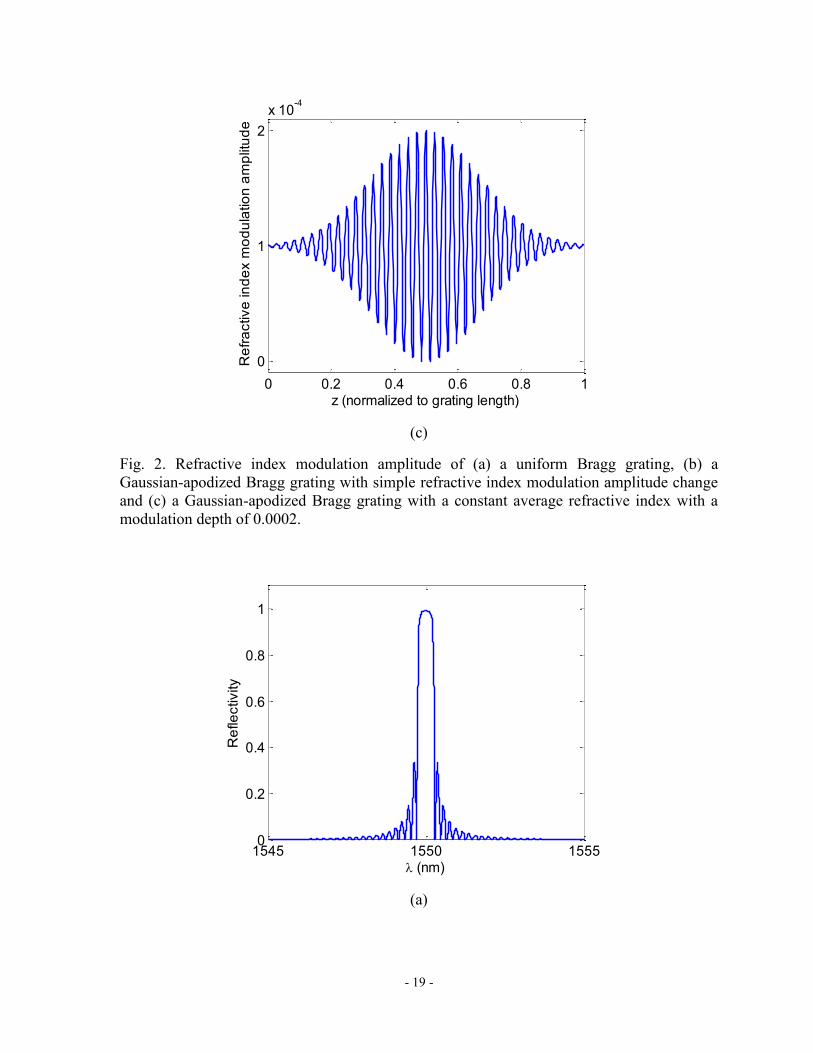
- 19 -

(c)

Fig. 2. Refractive index modulation amplitude of (a) a uniform Bragg grating, (b) a

Gaussian-apodized Bragg grating with simple refractive index modulation amplitude change

and (c) a Gaussian-apodized Bragg grating with a constant average refractive index with a

modulation depth of 0.0002.

(a)

0 0.2 0.4 0.6 0.8 1

0

1

2

x 10-4


Re

fra

ctive

in

de

x m

od

ula

tio

n a

mp

litu

de

1545 1550 15550

0.2

0.4

0.6

0.8

1

(nm)

Re

fle

ctivity

- 20 -

(b)

(c)

Fig. 3. Reflection spectrum of (a) a uniform Bragg grating, (b) a Gaussian-apodized Bragg

grating with simple refractive index modulation amplitude change and (c) a Gaussian-

apodized Bragg grating with a constant average refractive index.

1545 1550 15550

0.2

0.4

0.6

0.8

1

(nm)

Re

fle

ctivity

1545 1550 15550

0.2

0.4

0.6

0.8

1

(nm)

Re

fle

ctivity

- 21 -

(a)

(b)

1545 1550 15550

10

20

30

40

50

60

Gro

up

De

lay (

ps)

(nm)

1545 1550 15550

10

20

30

40

50

60

Gro

up

De

lay (

ps)

(nm)

- 22 -

(c)

Fig. 4. Group delay of (a) a uniform Bragg grating, (b) a Gaussian-apodized Bragg grating

with simple refractive index modulation amplitude change and (c) a Gaussian-apodized

Bragg grating with a constant average refractive index.

When dealing with gratings having arbitrary coupling constant and chirp, no simple

analytical solution exists. Also, these two variables cannot be separated as they collectively

affect the transfer function of a given grating. For simulation purposes of the chirped gratings

in this research project, the Transfer Matrix Method (TMM) is used [53] [71]-[73]. This

method was first used by Yamada [73] in 1987 to analyze optical waveguides.

In this method, the coupled mode equations of a Bragg grating are used to calculate the

output field of a short section of length δL of the grating. In this short section of grating, the

period of the grating, Λ(z), and the coupling constant, κ(z), are assumed to be constant. Thus,

this short section of a grating can be considered as a uniform grating. This uniform grating

1545 1550 15550

10

20

30

40

50

60

Gro

up

De

lay (

ps)

(nm)

- 23 -

can be viewed as a four-port device with two input- and two output-fields as depicted in Fig.

5.

Fig. 5. Diagram representing the transfer matrix method principle for a uniform grating.

The section of grating can be expressed as a transfer matrix linking the two input and two

output fields as

2/

2/

2/

2/

L

L

L

L

S

RT

S

R

.

(9)

The expression for the transfer matrix T, considering a uniform non-apodized grating of

length δL is given by (10).

)sinh(ˆ

)cosh()sinh(

)sinh()sinh(ˆ

)cosh(

LjLLj

LjLjLT

,

(10)

where 22 ̂ .

The transfer matrix method can be used to solve non-uniform gratings. This method is

effective in the analysis of the almost-periodic grating. A non-uniform Bragg grating can be

- 24 -

divided into many uniform sections. Each section is described by its transfer matrix Ti as

given in (10). The entire grating of length L is then approximated as the combined effect of

all uniform sections as shown in Fig. 6.

...

δL1 δL2 δLI-1 δLI

T1 T2 TI-1 TI

L

R-L/2

S-L/2

RL/2

SL/2

Fig. 6. Diagram showing the principle of the transfer matrix method for a non-uniform

grating.

The entire grating can be approximated to be

2/

2/

121

2/

2/...

L

L

II

L

L

S

RTTTT

S

R

,

(11)

where Ti are the transfer matrices of the sections, with i = 1 … I, and Rl and Sl are the fields

traveling in each direction, analyzed at a distance l from the reference point (usually defined

as the center of the SFBG).

When using the transfer matrix method, it is important to note that the number of sections, M,

cannot be arbitrarily large. The coupled-mode-theory approximations are not valid when a

uniform grating section is only a few grating periods long [73] unless the amplitude or period

- 25 -

is a slowly varying function along the length of the grating. In such cases, the TMM is

capable of handling a section length equal to a single grating period. Special care must be

taken to ensure that each section contains an integer number of grating periods in order to

have a smooth transition between sections. Not maintaining this condition can lead to a

deleterious effect outside the bandwidth of the grating. Finally, when simulating long chirped

gratings, care must be taken to allow adequate spectral resolution in order to calculate the

group delay accurately.

The following figures give the simulation results of linearly chirped gratings without

apodization and with a Gaussian apodization and back-scan. Both gratings have a total chirp

of 9 nm, which means that the Bragg wavelength of the grating at z = 0 and z = L, where L is

the length of the grating, differ by 9 nm.

(a)

1544 1546 1548 1550 1552 1554 15560

0.2

0.4

0.6

0.8

1

(nm)

Re

fle

ctivity

- 26 -

(b)

Fig. 7. Simulation results of the (a) reflection response and (b) delay induced by a 10-mm

long chirped Bragg grating with a Bragg wavelength chirp of 9 nm. The refractive index

modulation is equal to 10-4.

(a)

1544 1546 1548 1550 1552 1554 15560

20

40

60

80

100

120

Gro

up

De

lay (

ps)

(nm)

1544 1546 1548 1550 1552 1554 15560

0.2

0.4

0.6

0.8

1

(nm)

Re

fle

ctivity

- 27 -

(b)

Fig. 8. Simulation results of the (a) reflection response and (b) delay induced by a 10-mm

long Gaussian-apodized Bragg grating with a Bragg wavelength chirp of 9 nm. The refractive

index modulation is equal to 10-4.

2.1.2 Photosensitivity

Photosensitivity refers to a permanent change in the index of refraction induced by exposure

to light radiation [53]. Photosensitivity is commonly used to modulate the refractive index of

materials spatially and fabricate devices such as Bragg gratings. The fabrication process of

Bragg gratings will be described in Section 2.1.3.

Since the discovery of photosensitivity by Hill and al. [51] and the first demonstration of

grating formation in Ge-doped fibers, there have been considerable efforts in modeling and

increasing the photosensitivity in optical fibers. Many techniques and methods have been

developed to achieve just this in both optical fibers and planar glass structures. Such methods

1544 1546 1548 1550 1552 1554 15560

20

40

60

80

100

120

Gro

up

De

lay (

ps)

(nm)

- 28 -

include thermal-induced refractive index change, hydrogen loading, photosensitivity increase

by strain, and co-doping [53], [74].

2.1.3 Fabrication of Bragg gratings

In 1989, an important breakthrough in the Bragg grating fabrication was made by Gerry

Meltz and his coworkers [52]. The method they developed uses the superposition of

ultraviolet beams in order to produce an interference pattern which creates the grating.

Another technique for fabricating Bragg gratings consists of the two ultraviolet beams being

generated by exposing a periodic phase mask with a single UV beam. This section will

describe these two techniques for fabricating Bragg gratings in more details.

The holographic method of fabricating Bragg gratings uses a beam splitter to divide a single

ultraviolet beam. The two beams resulting from this splitter are brought together by

reflections from two mirrors. The fiber is then placed in the interference pattern created at the

intersection of the two UV beams. Fig. 9 shows the holographic method to write Bragg

gratings.

- 29 -

Fig. 9. Holographic method to write Bragg gratings.

With this method, the Bragg wavelength is given by

2sin

UV

UVeff

B

n

n

, (12)

where λUV is the wavelength of the UV beam, nUV is the refractive index of silica in the UV

region and θ is the mutual angle of the UV beams.

From this equation, it can be seen that the Bragg wavelength of a grating can be chosen

independently of the UV wavelength by controlling the mutual angle of the UV beams. This

method is better suited for short exposure times as mechanical vibrations and long path

lengths in the air affect the quality of the grating written if longer exposure time would be

used.

The second method to write Bragg gratings uses a phase mask as a component of the

interferometer. A phase mask is a relief grating which is often fabricated by holographic

- 30 -

exposure, but can also be fabricated by e-beam lithography in a fused silica plate. For grating

writing, the phase mask used is also called a zero-order-nulled phase mask as it is designed

so that minimum radiation is transmitted in the zeroth order and maximum radiation is

transmitted into the two first-order beams [75], [76]. Fig. 10 illustrates the concept of the

zero-order-nulled phase mask.

Fig. 10. Diffraction of a UV beam from a phase mask.

The period of the Bragg grating is related to the Bragg wavelength by the following relation

PMeffB n ,

(13)

where ΛPM is the period of the relief grating etched in the phase mask.

Photosensitivity, a property of a material indicating that it will react when exposed to light

energy, allows the writing of Bragg gratings in optical fibers and waveguides. This material

property is still being investigated as to which mechanisms are contributing to its effects. In

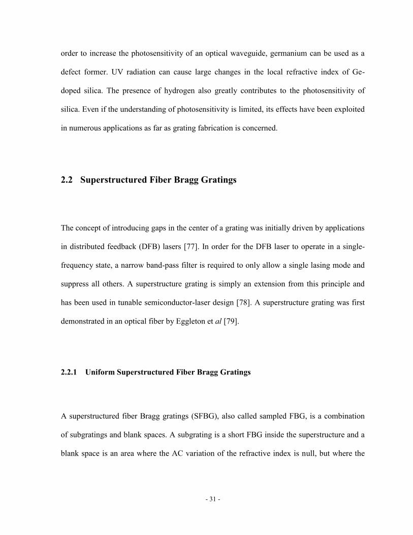
- 31 -

order to increase the photosensitivity of an optical waveguide, germanium can be used as a

defect former. UV radiation can cause large changes in the local refractive index of Ge-

doped silica. The presence of hydrogen also greatly contributes to the photosensitivity of

silica. Even if the understanding of photosensitivity is limited, its effects have been exploited

in numerous applications as far as grating fabrication is concerned.

2.2 Superstructured Fiber Bragg Gratings

The concept of introducing gaps in the center of a grating was initially driven by applications

in distributed feedback (DFB) lasers [77]. In order for the DFB laser to operate in a single-

frequency state, a narrow band-pass filter is required to only allow a single lasing mode and

suppress all others. A superstructure grating is simply an extension from this principle and

has been used in tunable semiconductor-laser design [78]. A superstructure grating was first

demonstrated in an optical fiber by Eggleton et al [79].

2.2.1 Uniform Superstructured Fiber Bragg Gratings

A superstructured fiber Bragg gratings (SFBG), also called sampled FBG, is a combination

of subgratings and blank spaces. A subgrating is a short FBG inside the superstructure and a

blank space is an area where the AC variation of the refractive index is null, but where the

- 32 -

DC component is often increased to reach a constant value throughout the superstructure.

Fig. 11 shows a possible refractive index profile of an SFBG.

SFBGs offer key advantages in many applications mainly because of the flexibility they offer

during their fabrication. By adjusting the parameters of the sampling function, it is possible

to achieve different reflection and transmission spectra as well as different dispersion profiles

with a single uniform phase mask [7] [8] [9].

As shown in Fig. 11, the SFBG is composed of N sections, with each section consisting of a

subgrating and a blank space. The length of a section is referred to as the sampling period, Z0,

and the length of a subgrating is represented by Ls.

SubgratingBlank

Space

z (mm)

Period

δneff

{1 2 3 4 5

... ...N-1 N

Fig. 11. Refractive index profile of a superstructured fiber Bragg grating made of N sections.

The spectrum of an SFBG is analogous to the Fourier transform of its spatial profile under a

weak refractive index modulation approximation. Thus, following Fourier transform theory,

the uniform sampling of an FBG in the spatial domain will lead to a periodic spectrum.

- 33 -

Fig. 12 shows the spectrum of a uniformly sampled SFBG with raised-cosine apodization as

well as the refractive index profile along the length of the optical fiber, z.

(a)

(b)

1545 1550 15550

0.2

0.4

0.6

0.8

1

(nm)

Re

fle

ctivity

1545 1550 15550

50

100

150

200

Gro

up

De

lay (

ps)

(nm)

- 34 -

(c)

Fig. 12. Amplitude response (a), group delay response (b) and refractive index profile (c) of a

uniformly sampled SFBG, with Z0 = 0.68 mm, Ls = 0.36 mm and N = 40. The blue rectangles

of the refractive index profile are in fact sinusoidal with a very small period.

The spatial profile of a uniform SFBG along the z-axis can be expressed by the sum of an

infinite number of Dirac delta functions evenly spaced along the z-axis convoluted by a

rectangular function representing the subgrating, all of which would be multiplied by the

apodization profile. Mathematically, this is expressed as

2

*1 0sn

L

zrectZnzzAzP ,

(14)

where A(z) is the apodization profile, δ(z) is the Dirac delta function, Z0 is the sampling

period, Ls is the subgrating length and ZL is the total superstructure length. The asterisk “*”

denotes the convolution operation.

In the case of a uniformly apodized SFBG, we have

0 5 10 15 20

1.4470

1.4471

1.4472

1.4473

1.4474

x (mm)

n

- 35 -

2LZ

zrectzA , (15)

where ZL is the total superstructure length.

Fig. 13(a) shows a representation of (14) with the apodization profile as defined in (15) as

well as the spatial representation of different key points and Fig. 13(b) shows the equivalent

representation in the Fourier domain.

1

n

Znz 0

× *

2sL

zrect

-20 -10 0 10 200

0.5

1

z (mm)

... 0 ...0

0.5

1

z (mm)

- +

... 0 ...0

0.5

1

z (mm)

- + ... 0 ...0

0.5

1

z (mm)

- +

×

... 0 ...0

0.5

1

z (mm)

- +

2LZ

zrect

-20 -10 0 10 200

0.5

1

z (mm)

-20 -10 0 10 200

0.5

1

z (mm)

(a)

- 36 -

1545 1550 15550

0.5

1

(nm)

1545 1550 15550

0.5

1

(nm)

1545 1550 15550

0.5

1

(nm)

1545 1550 15550

0.5

1

(nm)

1545 1550 15550

0.5

1

(nm)

1545 1550 15550

0.5

1

(nm)

*

1545 1550 15550

0.5

1

(nm)

δ(λ)

*×

n Z

n

0

2

sLincs

2

LZincs

(b)

Fig. 13. Spatial (a) and spectral (b) relationship in a superstructured fiber Bragg grating with

uniform sampling period and uniform apodization.

Applying Fourier Transform identities to the spatial representation of the SFBG, the

amplitude reflection coefficient of an SFBG, under the weak refractive index modulation

approximation, can be defined as

2*ˆˆ

0

s

n

Lncsi

Z

nAP

,

(16)

where Â(λ) is the Fourier transform of the apodization profile of the superstructure.

In the case of a uniformly apodized SFBG, Â(λ) can be expressed as

- 37 -

2ˆ LZ

incsA

. (17)

It is possible to deduce some physical profile to spectral response mapping from Fig. 13(a)

and (b) by using simple Fourier transform properties. The following paragraphs summarize

these.

The periodic repetition of the spectrum, typical of SFBGs, is linked to the sampling period of

the superstructure and the spacing between the different orders is inversely proportional to

the sampling period. Fig. 14 shows the effect of the sampling period on the amplitude and

group delay response of an SFBG for three (3) different values. It is also important to note

that the group delay response of the SFBG is also affected by the change in sampling period.

Because the sampling period affects the physical location of the subgratings, and thus the

physical structure, the light reflected has to travel to the subgratings before being reflected.

When the subgratings are close to one another (lower value of Z0), the average group delay is

thus less than when the subgratings are spaced further to on another (higher value of Z0).

- 38 -

(a)

(b)

1545 1550 15550

0.2

0.4

0.6

0.8

1

(nm)

Re

fle

ctivity

1545 1550 15550

100

200

300

400

500

600

700

Gro

up

De

lay (

ps)

(nm)

- 39 -

(c)

(d)

1545 1550 15550

0.2

0.4

0.6

0.8

1

(nm)

Re

fle

ctivity

1545 1550 15550

100

200

300

400

500

600

700

Gro

up

De

lay (

ps)

(nm)

- 40 -

(e)

(f)

Fig. 14. Effect of the sampling period, Z0, on the spectrum of an SFBG. For all SFBGs, Ls =

0.36 mm, N = 40. For (a) and (b), Z0 = 0.50 mm; for (c) and (d), Z0 = 1.25 mm; for (e) and

(f), Z0 = 2.00 mm. (a), (c) and (e) show the amplitude response of the SFBG; (b), (d) and (f),

the group delay response or the corresponding SFBG. The SFBGs have a raised-cosine

apodization applied to their superstructure profile.

1545 1550 15550

0.2

0.4

0.6

0.8

1

(nm)

Re

fle

ctivity

1545 1550 15550

100

200

300

400

500

600

Gro

up

De

lay (

ps)

(nm)

- 41 -

The envelope multiplying the amplitude of the spectrum is a function of the subgrating

length. The shorter the subgrating is, the broader the multiplying envelope gets. As shown in

equations (14) and (16), the convolution of the subgrating profile translates in a

multiplication in the spectral domain. In the case of a rectangle function in the spatial

domain, the corresponding sinc function in the spectral domain will contain sidelobes that are

spaced inversely proportionately to the width of the subgrating. Fig. 15 shows the reflectivity

and group delay responses of SFBGs with different subgrating lengths.

(a)

1545 1550 15550

0.2

0.4

0.6

0.8

1

(nm)

Re

fle

ctivity

- 42 -

(b)

(c)

1545 1550 15550

100

200

300

400

500

600

700

Gro

up

De

lay (

ps)

(nm)

1545 1550 15550

0.2

0.4

0.6

0.8

1

(nm)

Re

fle

ctivity

- 43 -

(d)

(e)

1545 1550 15550

100

200

300

400

500

600

700

Gro

up

De

lay (

ps)

(nm)

1545 1550 15550

0.2

0.4

0.6

0.8

1

(nm)

Re

fle

ctivity

- 44 -

(f)

Fig. 15. Effect of the subgrating length, Ls, on the spectrum of an SFBG. For all SFBGs, Z0 =

2 mm, N = 40. For (a) and (b), Ls = 0.20 mm; for (c) and (d), Ls = 0.30 mm; for (e) and (f), Ls

= 0.4 mm. (a), (c) and (e) show the amplitude response of the SFBG; (b), (d) and (f), the

group delay response or the corresponding SFBG. The SFBGs have a raised-cosine

apodization applied to their superstructure profile.

The subgrating length, Ls, changes the envelope that modulates the amplitude spectrum. The

group delay response, on the other hand, keeps approximately the same value in the pass

band of the SFBG and this, for each value of Ls.

Each subgrating can also be apodized, which will shape the envelope of the amplitude

spectrum. The same effects as for regular FBGs can be observed, e.g. a raised-cosine or sinc

apodization will lead to lower sidelobes, etc. The sidelobes concerned are found on the

envelope of the spectrum and not on the individual spectral orders. The sidelobes found on

the spectral orders will be discussed later. Fig. 16 shows the reflectivity and group delay

responses of SFBGs with different apodization profiles applied to the subgratings.

1545 1550 15550

100

200

300

400

500

600

700

Gro

up

De

lay (

ps)

(nm)

- 45 -

(a)

(b)

1545 1550 15550

0.2

0.4

0.6

0.8

1

(nm)

Re

fle

ctivity

1545 1550 15550

200

400

600

800

1000

Gro

up

De

lay (

ps)

(nm)

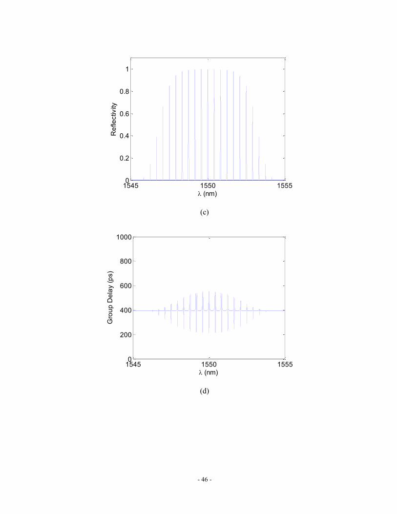
- 46 -

(c)

(d)

1545 1550 15550

0.2

0.4

0.6

0.8

1

(nm)

Re

fle

ctivity

1545 1550 15550

200

400

600

800

1000

Gro

up

De

lay (

ps)

(nm)

- 47 -

(e)

(f)

Fig. 16. Effect of the subgrating apodization on the spectrum of an SFBG. For all SFBGs, Z0

= 2 mm, Ls = 0.36 mm and N = 40. For (a) and (b), the subgratings are uniformly apodized;

for (c) and (d), raised-cosine apodized; for (e) and (f), Gaussian apodized. (a), (c) and (e)

show the amplitude response of the SFBG; (b), (d) and (f), the group delay response or the

corresponding SFBG. The SFBGs have a raised-cosine apodization applied to their

superstructure profile.

1545 1550 15550

0.2

0.4

0.6

0.8

1

(nm)

Re

fle

ctivity

1545 1550 15550

200

400

600

800

1000

Gro

up

De

lay (

ps)

(nm)

- 48 -

Finally, the shape of each Fourier order is dependent on the profile of the superstructure. A

rectangular superstructure profile gives a “sinc” profile for each spectral order, with the

associated side lobes. Applying an apodization profile to the superstructure will lead to

orders with lower side lobes, for example. In all previous examples, a raised-cosine

apodization profile was applied to the SFBGs simulated. Fig. 17 shows the reflectivity and

group delay responses of SFBGs with different apodization profiles applied to the

superstructure.

(a)

(b)

1545 1550 15550

0.2

0.4

0.6

0.8

1

(nm)

Re

fle

ctivity

1550 1550.1 1550.2 1550.3 1550.4 1550.50

0.2

0.4

0.6

0.8

1

(nm)

Reflectivity

1545 1550 15550

200

400

600

800

1000

Gro

up

De

lay (

ps)

(nm)1550 1550.1 1550.2 1550.3 1550.4 1550.50

100

200

300

400

500

600

700

800

900

1000

Gro

up D

ela

y (

ps)

(nm)

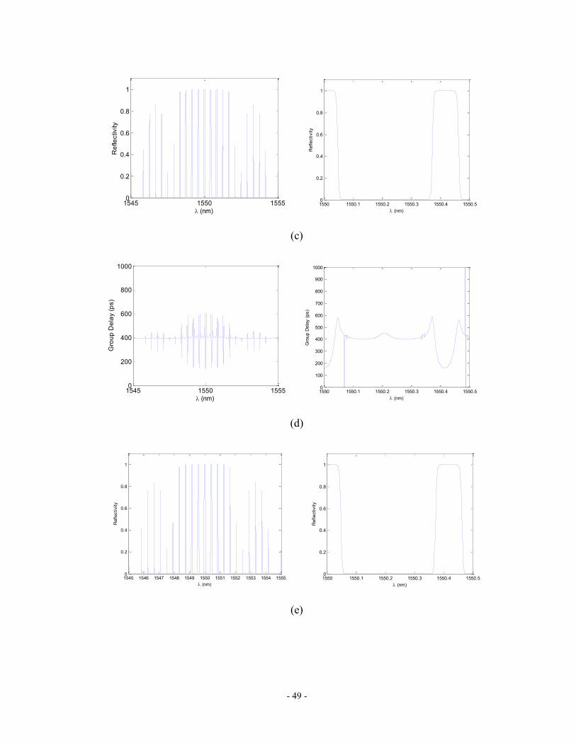
- 49 -

(c)

(d)

(e)

1545 1550 15550

0.2

0.4

0.6

0.8

1

(nm)

Re

fle

ctivity

1550 1550.1 1550.2 1550.3 1550.4 1550.50

0.2

0.4

0.6

0.8

1

(nm)

Reflectivity

1545 1550 15550

200

400

600

800

1000

Gro

up

De

lay (

ps)

(nm)1550 1550.1 1550.2 1550.3 1550.4 1550.50

100

200

300

400

500

600

700

800

900

1000

Gro

up D

ela

y (

ps)

(nm)

1545 1546 1547 1548 1549 1550 1551 1552 1553 1554 15550

0.2

0.4

0.6

0.8

1

(nm)

Reflectivity

1550 1550.1 1550.2 1550.3 1550.4 1550.50

0.2

0.4

0.6

0.8

1

(nm)

Reflectivity

- 50 -

(f)

Fig. 17. Effect of the superstructure apodization on the spectrum of an SFBG. For all SFBGs,

Z0 = 2 mm, Ls = 0.36 mm and N = 40. For all SFBGs, the subgratings are uniformly

apodized. For (a) and (b), the superstructure is uniformly apodized; for (c) and (d), raised-

cosine apodized; for (e) and (f), Sine-squared apodized. (a), (c) and (e) show the amplitude

response of the SFBG; (b), (d) and (f), the group delay response or the corresponding SFBG.

To summarize, this section demonstrated the mapping of spatial parameters in the

superstructure refractive index profile to corresponding spectral parameters.

2.2.2 Equivalent Phase-Shifted Superstructured Fiber Bragg Gratings

As the previous section demonstrated, the shape of the superstructure impacts the shape of

spectral orders. It has been demonstrated that applying an apodization profile on the

superstructure yields spectral orders with lower sidelobes. Following this train of thought,

shaping the superstructure in ways that were traditionally done on the refractive index profile

of an FBG will result in similar FBG responses in the orders of the SFBG. One potential

1545 1550 15550

200

400

600

800

1000

Gro

up

De

lay (

ps)

(nm)1550 1550.1 1550.2 1550.3 1550.4 1550.50

100

200

300

400

500

600

700

800

900

1000

Gro

up D

ela

y (

ps)

(nm)

- 51 -

shaping method of the superstructure is to introduce a phase-shift. This has been first

demonstrated by Y. Dai et al. in 2004 [10].

The technique consists in introducing a π-phase shift in the sampling function of the

superstructure. Doing so results in an equivalent π-phase shift in the odd orders of the

spectrum of the SFBG, the stronger orders being the +/-1st orders. Fig. 18 shows the

amplitude and phase response of an SFBG with an equivalent phase shift in its sampling

period.

(a)

1545 1550 15550

0.2

0.4

0.6

0.8

1

(nm)

Re

fle

ctivity

- 52 -

(b)

Fig. 18. (a) Amplitude and (b) group delay response of a 40-section SFBG with an equivalent

π-phase shift in its 20th section. The SFBG is sine-square apodized.

Fig. 19 shows the refractive index profile of the SFBG with an equivalent phase shift in its

sampling period. The SFBG is sine-square apodized with its average refractive index set to a

constant value throughout the superstructure.

Fig. 19. Refractive index profile of a 40-section SFBG with an equivalent π-phase shift in its

20th section. The SFBG is sine-square apodized.

1545 1550 15550

100

200

300

400

500

Gro

up

De

lay (

ps)

(nm)

0 5 10 15 20

1.447

1.4471

1.4472

1.4473

1.4474

1.4475

x (mm)

- 53 -

2.2.3 Equivalent Chirp in Superstructured Fiber Bragg Gratings

Equivalent chirp in a SFBG is achieved by chirping the sampling profile of the

superstructure. A linear chirp coefficient in the sampling profile gives approximately a linear

group delay response in the high orders of the spectral profile.

Fig. 20 shows the amplitude and phase response of an SFBG with an equivalent chirp in its

sampling period.

(a)

1545 1550 15550

0.2

0.4

0.6

0.8

1

(nm)

Re

fle

ctivity

- 54 -

(b)

Fig. 20. (a) Amplitude and (b) group delay response of a 40-section SFBG with an equivalent

chirp in its sampling profile. The SFBG is sine-square apodized.

Fig. 21 shows the refractive index profile of the SFBG with an equivalent chirp in its

sampling period. The SFBG is sine-square apodized with its average refractive index set to a

constant value throughout the superstructure.

Fig. 21. Refractive index profile of a 40-section SFBG with an equivalent chirp in its

sampling profile. The SFBG is sine-square apodized.

1545 1550 15550

50

100

150

200

250

300

350

Gro

up

De

lay (

ps)

(nm)

0 5 10 15 20 25 30

1.447

1.4472

1.4474

x (mm)

- 55 -

2.3 Phased Array Antennas

Antenna arrays are essentially a group of simple antennas called the array elements that are

combined together to operate as a single antenna with a desired radiation pattern. The array

elements may be many kind of antenna, such as dipoles, dielectric resonators or microstrip

patches to only name a few. In order to shape the overall radiation pattern of the linked

elements, several parameters can be controlled. These parameters include the number of

elements in the array, the spatial location of each element with respect to the others, the

orientation of each element as well as the parameters of the feed signals.

Since the feed signals parameters can be used to achieve a particular radiation pattern of the

antenna array, it is then possible to dynamically control the shape of this radiation pattern.

Furthermore, this control can be done without having any physical movement from the

antenna. In other words, one possible extension of this is the possibility to scan the main lobe

of the radiation pattern without moving the antenna. This is the principle behind phased array

antennas.

2.3.1 Two-elements array

Let us consider the case of an antenna array composed of two array elements as a simple

theoretical case. The elements are spaced by a distance of s and are placed along the z-axis as

shown in Fig. 22.

- 56 -

0 y

z

s/2

-s/2

Fig. 22. Antenna array composed of two elements.

If we assume that each element is an isotropic source, i.e., the radiation pattern of each

element is spherical with uniform amplitude, the electric field of each element can be

expressed as

)(1 krjer

E.

(18)

For the antenna array considered in Fig. 22, the total electric field in the far field would be

the sum of the individual isotropic elements

)2/(

2

)2/(

1

2121

11

krjkrje

re

rEEE

,

(19)

where r1 and r2 are defined in Fig. 23 and β/2 and –β/2 are the phase of the feed signals.

- 57 -

0 y

z

s/2

-s/2

r1

r2

r

p

θ

Fig. 23. Electric field in the far field.

In the far field, the following approximations can be made:

for the amplitude terms:

21

(20)

rrr 21

(21)

for the phase terms:

21

(22)

)cos(2

),cos(2

21 s

rrs

rr (23)

Thus, the total electric field in the far-field region can be expressed as

)2/)cos(2/cos(2

skr

eE

jkr

. (24)

- 58 -

The first part of this expression, r

e jkr

, corresponds to the element pattern (for an isotropic

source) and the second part is called the array factor. Thus, for antenna arrays, the total array

pattern is the product of the element pattern and the array factor

FactorArrayPatternElementPatternArray . (25)

In general, the array factor is considered alone when discussing antenna arrays. This is a way

of “normalizing” the effect of the array regardless of the type of antenna used.

2.3.2 N-element linear array

The concept of a linear array can be extended from two elements to M elements. The

elements are uniformly spaced and located at positions (m-1) s for m = 1, 2, 3, …, M along

the z axis. If each element is excited by a current Im, then the array factor can be expressed as

cos)1( skmj

m

m

m

m eIAFAF

. (26)

If the exciting currents have a magnitude and phase given by

mj

mm eAI

, (27)

and if the phase βm is linear with respect to m, it can be expressed as

)1( mm . (28)

- 59 -

If the current has the same amplitude A for each element, the array factor can then be

expressed as [48]

)1(

mj

m

eAAF , (29)

where cossk .

The normalized amplitude of the array factor can thus be shown to be

)2/sin(

)2/sin()(

M

Maf , (30)

where the lowercase af represents a normalized value.

2.3.3 Planar array

It is possible to further extend the concept of linear arrays to planar arrays. These arrays can

be represented either as a linear combination of linear arrays (for a rectangular lattice) or as a

combination of elements arranged in a regular pattern. These planar arrays present an even

greater degree of control over the far-field pattern. The elements in planar arrays can be

arranged in various configurations as depicted in Fig. 24.

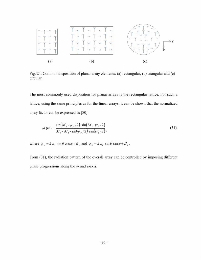
- 60 -

z

y

(a) (b) (c)

Fig. 24. Common disposition of planar array elements: (a) rectangular, (b) triangular and (c)

circular.

The most commonly used disposition for planar arrays is the rectangular lattice. For such a

lattice, using the same principles as for the linear arrays, it can be shown that the normalized

array factor can be expressed as [80]

2sin2sin

2sin2sin)(

zyzy

zzyy

MM

MMaf

,

(31)

where yyy sk cossin and zzz sk sinsin .

From (31), the radiation pattern of the overall array can be controlled by imposing different

phase progressions along the y- and z-axis.

- 61 -

2.3.4 Far-field radiation pattern

In this section, only linear arrays will be considered in order to simplify the theory presented

and still give a general overview of the behavior of phased array antennas. It has been

demonstrated that the normalized array factor for such antennas is given by

)2/sin(

)2/sin()(

M

Maf , (32)

where cossk . k is the wave number in free space (which is equal to RF2 and

where λRF is the free space wavelength).

From the equations, the angle and the shape of the main beam of the antenna, θ, can be

controlled by adjusting the distance between the antennas’ array elements, the phase

progression in the feed signals and by changing the number of elements. Fig. 25 shows the

influence of the distance between elements on the array pattern when there is no phase

progression.

- 62 -

Fig. 25. Normalized radiation pattern for different element spacing (β = 0°, M = 12).

As it can be seen, the spacing between elements influences only the directivity and the width

of the main lobe. This next figure shows the influence of the number of elements on the

normalized far-field radiation pattern when there is no phase progression and when the

spacing between elements is kept constant and equal to λRF/4.

0.2

0.4

0.6

0.8

1

30

210

60

240

90

270

120

300

150

330

180 0

s = RF

/8

s = RF

/4

s = 3RF

/8

s = RF

/2

- 63 -

Fig. 26. Normalized radiation pattern for different number of elements (β = 0°, s = λRF/4).

From Fig. 26, the number of elements also influences the overall shape of the radiation

pattern and the directivity of the antenna and the width of the main lobe. Along with the

element spacing, the number of elements also plays a role in determining the number of

sidelobes present in the array factor. Fig. 27 shows the influence of the phase progression on

the far-field radiation pattern when the number of elements, M, and the distance between

them, s, are kept constant and equal to 12 and λRF/4 respectively.

0.2

0.4

0.6

0.8

1

30

210

60

240

90

270

120

300

150

330

180 0

M = 2

M = 4

M = 6

M = 10

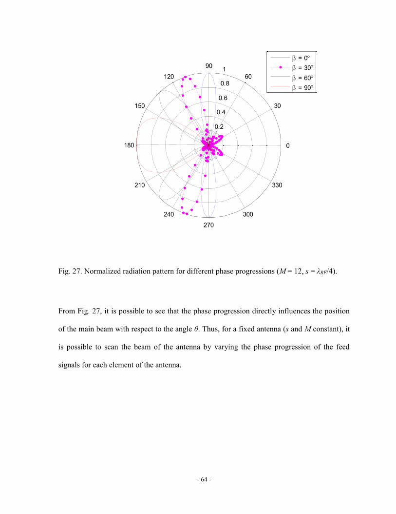
- 64 -

Fig. 27. Normalized radiation pattern for different phase progressions (M = 12, s = λRF/4).

From Fig. 27, it is possible to see that the phase progression directly influences the position

of the main beam with respect to the angle θ. Thus, for a fixed antenna (s and M constant), it

is possible to scan the beam of the antenna by varying the phase progression of the feed

signals for each element of the antenna.

0.2

0.4

0.6

0.8

1

30

210

60

240

90

270

120

300

150

330

180 0

= 0

= 30

= 60

= 90

- 65 -

2.3.5 True time delay

Phase shifters are components which adjust the appropriate phase of each feed signal going

to the radiating elements of a phased array antenna. Different approaches to realizing such

components have been proposed and tested in the past (e.g., [85]-[88]). Some of these

approaches are very simple in nature while other are quite complex. A main criterion directly

related to the complexity of the phase shifters is the tunability of such devices. In other

words, the need to dynamically scan the main lobe of the antenna radiation pattern increases

the level of complexity required for the phase shifters.

Conventional phase shifters introduce a certain phase to the incoming signals regardless of

the frequency of this signal. The above theory presented on phased array antennas were

considering such devices as the phase progression β was considered constant for all

frequencies.

One major drawback of this approach in realizing phased array antennas is a phenomenon

known as beam squint. This phenomenon is characterized by the position of the main lobe of

the array factor being oriented at different angles, θ, for different signal frequencies. In other

words, the energy associated with different frequencies is oriented in different directions and

thus restricts the use of the antenna for narrowband applications. The following graphs give

an example of an antenna of 6 elements separated by a distance, s, of 0.75 cm operating at a

central frequency f0 of 15 GHz. For the purposes of illustrating the beam squint effect, the

bandwidth of the antenna will be assumed to be 10 GHz. Thus, the behavior of the antenna

will be studied for the frequencies from 10 to 20 GHz.

- 66 -

The far-field radiation pattern of the array factor (considering isotropic elements) for the

central frequency f0 is given in Fig. 28.

Fig. 28. Array factor for a PAA of M = 6 elements with s = 0.75 cm at f0 = 15 GHz.

Fig. 29 illustrates the far-field radiation pattern of the array factor for frequencies between 10

and 20 GHz by intervals of 2 GHz for a phase progression of β = π/2.

0.2

0.4

0.6

0.8

1

30

210

60

240

90

270

120

300

150

330

180 0

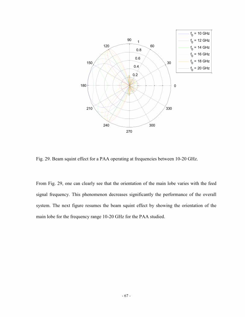
- 67 -

Fig. 29. Beam squint effect for a PAA operating at frequencies between 10-20 GHz.

From Fig. 29, one can clearly see that the orientation of the main lobe varies with the feed

signal frequency. This phenomenon decreases significantly the performance of the overall

system. The next figure resumes the beam squint effect by showing the orientation of the

main lobe for the frequency range 10-20 GHz for the PAA studied.

0.2

0.4

0.6

0.8

1

30

210

60

240

90

270

120

300

150

330

180 0

f0 = 10 GHz

f0 = 12 GHz

f0 = 14 GHz

f0 = 16 GHz

f0 = 18 GHz

f0 = 20 GHz

- 68 -

Fig. 30. Angle of the main lobe for a PAA operating frequencies between 10-20 GHz.

From Fig. 30, it can be seen that the main lobe orientation varies from approximately 120° to

180° over the range of frequencies observed.

A way to eliminate the beam squint is to use a method called true time-delay. This method

consists of introducing a time delay ∆t progression to the feed signals instead of a phase

progression. This time delay is constant for all frequencies and thus translates into a variable

phase shift with respect to frequency. In free space, this phase shift can be expressed as

tf 02 . (33)

10 11 12 13 14 15 16 17 18 19 20120

130

140

150

160

170

180

f0 (GHz)

()

- 69 -

The following figures use the same PAA example as for the conventional phase shifters (M =

6 elements separated by a distance, s, of 0.75 cm) operating at the same central frequency f0

of 15 GHz. The behavior of the antenna is studied for the frequencies from 10 to 20 GHz.

This time, true time-delays components are used instead of conventional phase shifters.

These elements introduce a time progression of ∆t = 16.67 ps which corresponds to the same

phase of π/2 at a frequency of 15 GHz. Fig. 31 illustrates the far-field radiation pattern of the

array factor for frequencies between 10 and 20 GHz by intervals of 2 GHz which uses true

time-delay components.

Fig. 31. Array factor of a PAA operating at frequencies between 10-20 GHz.

0.2

0.4

0.6

0.8

1

30

210

60

240

90

270

120

300

150

330

180 0

f0 = 10 GHz

f0 = 12 GHz

f0 = 14 GHz

f0 = 16 GHz

f0 = 18 GHz

f0 = 20 GHz

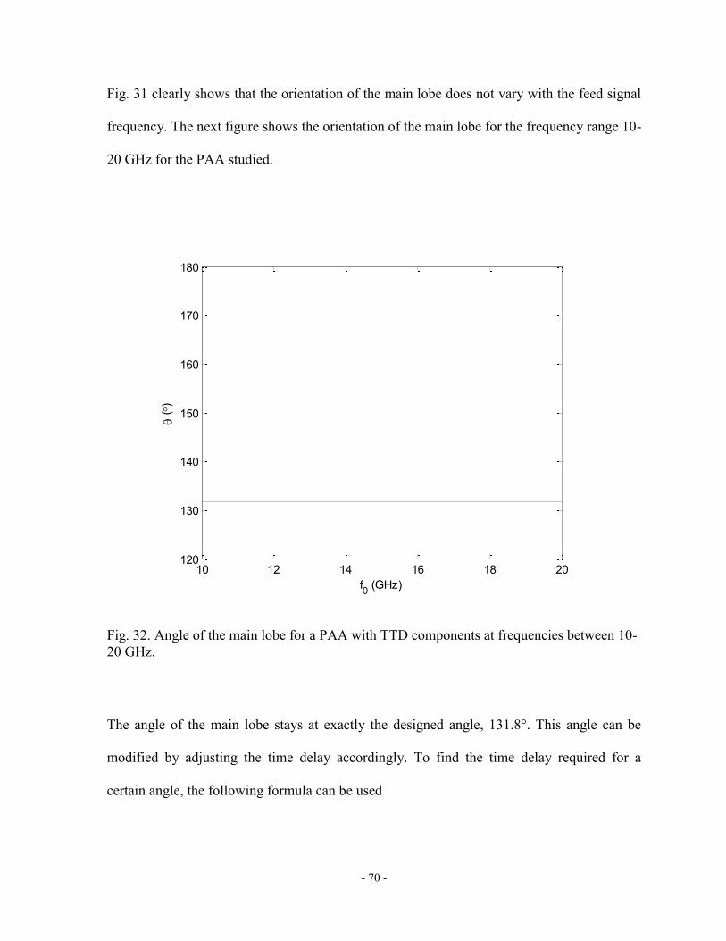
- 70 -

Fig. 31 clearly shows that the orientation of the main lobe does not vary with the feed signal

frequency. The next figure shows the orientation of the main lobe for the frequency range 10-

20 GHz for the PAA studied.

Fig. 32. Angle of the main lobe for a PAA with TTD components at frequencies between 10-

20 GHz.

The angle of the main lobe stays at exactly the designed angle, 131.8°. This angle can be

modified by adjusting the time delay accordingly. To find the time delay required for a

certain angle, the following formula can be used

10 12 14 16 18 20120

130

140

150

160

170

180

f0 (GHz)

()

- 71 -

cosc

st

, (34)

where c is the speed of light in vacuum and s is the spacing between the antenna elements.

It can be noticed that the time delay required to orient the main lobe of the antenna does not

depend on the frequency, which proves furthermore that TTD components do not introduce

“squint” in the far-field pattern of the antenna array.

2.3.6 Photonic true time delay

Traditionally, feed networks and phase shifters for phased array antennas were using

microwave electronic components. This was the most intuitive approach since antennas work

on an electrical driving source. With the advancement of technology, severe limitations were

observed in electrical devices. For example, copper wires display high losses at high

frequencies resulting in a limited bandwidth for the feed signals. Furthermore, electrical

beamforming networks have a relatively high weight, thus limiting their use in airborne

applications.

Optical components, with key advantages such as immunity to electromagnetic interference,

low loss, small size and light weight (especially if integrated optics are used), are being

considered as a promising alternative for wideband phased array antennas. Many photonic

true time-delay techniques have been proposed in the past. An important criterion for a good

- 72 -

true time-delay unit is the ability of tuning the time delay in order to steer the main lobe of

the antenna.

- 73 -

PHOTONIC TRUE-TIME DELAY BEAMFORMING BASED ON

SUPERSTRUCTURED FIBER BRAGG GRATINGS WITH LINEARLY

INCREASING EQUIVALENT CHIRPS

The key components in a true time-delay beamforming network are the delay lines. These

delay lines are required to produce accurate time delays and offer a large tunability. The TTD

beamforming network under consideration is depicted in Fig. 33. Electrical components are

presented in bold. The output of a tunable laser source (TLS) is sent to an external electro-

optic modulator (EOM) through a polarization controller (PC). At the EOM stage, the optical

carrier is intensity modulated by an RF signal. The modulated light signal is then divided

equally into four branches by a 1:4 optical splitter. Each output branch is connected to a

three-port optical circulator followed by a SFBG. The SFBG will introduce a time delay to

the optical signal. The time delay introduced varies as a function of the wavelength of the

optical carrier. The reflected optical signals from the SFBGs are then applied to a

photodetector array. The time delays caused by the SFBGs are then translated into different

beam steering angles at the PAA.

- 74 -

PD

PD

PD

PD

A

A

A

A

TLS PC EOM

Power

Splitter

SFBG 1

SFBG 2

SFBG 3

SFBG 4

Fig. 33. True time-delay beamforming network using a Bragg grating prism composed of

SFBGs.

3.1 SFBG with equivalent chirp in their sampling periods for use in TTD

applications

To design SFBGs for TTD applications, it is necessary to be able to determine the dispersion

associated with the physical design parameters of these gratings. The proposed TTD

beamformer based on an SFBG prism requires the design and fabrication of M SFBGs with

each having a specific dispersion value. While no simple closed form expression exists to

characterize the amplitude and phase response of an SFBG, it is possible to make a few

approximations in order to come up with an equation describing the influence of certain

parameters of the superstructure on the dispersion in a given Fourier order.

When uniform sampling is used, we have 0ZnZ . The spacing between two adjacent orders

is approximated by [89]

- 75 -

0

2

2 Zneff

B , (35)

where λB is the Bragg wavelength, neff is the effective refractive index of the fiber, and Z0 is

the uniform sampling period.

If we assume a linear chirp in the sampling function as a function of the physical position

along the grating length, we have

zZzZ 10 1 , (36)

where Z0 is defined as the initial sampling period and ς1 is the linear chirp coefficient. When

ς1 is equal to 0, Z(z) = Z0 for all values of z. This corresponds to a uniform sampling

function. Otherwise, when ς1 is non-zero, the period will be chirped along the length, z, of the

superstructure.

The period of first sample, at z = 0 is equal to

010 010]0[ ZZZZ . (37)

The period of the second sample, taken at the end of the first sample is equal to

0100 1]1[ ZZZZZ . (38)

Following the same logic, the period of the third sample is calculated at a value of z equal to

the sum of the periods of the previous samples and is equal to

0100100 111 ZZZZZz , (39)

201001010010 111111]2[ ZZZZZZZZZ (40)

- 76 -

From (36) – (40), it can be found that

nZZnZ 010 1 . (41)

The total length of a linearly chirped SFBG can be expressed as the sum of all periods of the

superstructure, as

n

L nZZ

. (42)

Substituting (41) into (42), we get

1

0

010 1N

n

n

L ZZZ . (43)

By exploiting geometric series identities, (43) can be expressed as

11

101

1

N

L ZZ

, 11 01 Z . (44)

The equivalent chirp of the superstructure can then be expressed as

11 01

110

N

ZZ

Z

m

dz

dN

, (45)

where iZ

is given by (35) and m is the Fourier order of the SFBG spectrum under

investigation.

From (41), we can find ZN-1 as

1

0101 1

N

N ZZZ . (46)

- 77 -

By substituting (35) and (46) into (45) and after simplification, we get the following

expression for the equivalent chirp:

111

11

20101

0101

0

1

2

NN

N

eff

B

ZZ

ZZ

Zn

m

dz

d

. (47)

It is known that the dispersion of a linearly chirped FBG can be approximated by

12

dz

d

c

nD

eff , (48)

where c is the speed of light in vacuum (3 × 108 m/s). It is then possible to approximate the

dispersion in the first order of a linearly equivalent-chirped SFBG as

0101

0101

1

2

0

2

11

1114

ZZ

ZZ

mc

ZnD

N

NN

B

eff

. (49)

Four equivalent-chirped SFBGs are used in the fabrication of the TTD beamformer. Their

design parameters are summarized in Table 1.

P0 (mm) Ls (mm) ς1 N

SFBG-1 0.6 0.3 2.564×10-2 40

SFBG-2 0.6 0.3 2.040×10-2 50

SFBG-3 0.6 0.3 1.695×10-2 60

SFBG-4 0.6 0.3 1.449×10-2 70

Table 1. Superstructured fiber Bragg gratings parameters. P0: Initial period; Ls: Section

length; ς1: linear equivalent chirp parameter; N: number of periods in the superstructure.

- 78 -

Based on these parameters, it is possible to calculate the theoretical dispersion of these

SFBGs in the -1st order by using (49) which gives the following values: SFBG-1: d1 = 510.1

ps/nm; SFBG-2: d2 = 637.2 ps/nm; SFBG-3: d3 = 764.2 ps/nm and SFBG-4: d4 = 891.3

ps/nm. From these values, it is clear that the dispersions linearly increase with the index of

the SFBGs which explains the choice of superstructure parameters.

Fig. 34 shows the simulated amplitude and group delay response of the SFBGs, along with

the theoretical average dispersion. As no close form mathematical expression exists to

characterize an SFBG, numerical simulations are usually used to evaluate the effects of the

chirp coefficients on the transmission and reflection spectra of an SFBG. The transfer matrix

method (TMM) is very well suited for simulation of such gratings and was used in this

analysis [55].

(a)

1557.1 1557.2 1557.3-10

-8

-6

-4

-2

0

Re

fle

ctivity (

dB

)

1557.1 1557.2 1557.30

140

280

420

560

700

Gro

up

De

lay (

ps)

(nm)

- 79 -

(b)

(c)

1557.1 1557.2 1557.3-10

-8

-6

-4

-2

0

Re

fle

ctivity (

dB

)

1557.1 1557.2 1557.30

140

280

420

560

700

Gro

up

De

lay (

ps)

(nm)

1557.1 1557.2 1557.3-10

-8

-6

-4

-2

0

Re

fle

ctivity (

dB

)

1557.1 1557.2 1557.30

140

280

420

560

700

Gro

up

De

lay (

ps)

(nm)

- 80 -

(d)

Fig. 34. Reflectivity (solid line) and simulated (solid line) and theoretical (dotted line) group

delay response for the superstructured fiber Bragg gratings used in the true-time delay prism.

The parameters of the SFBGs are given in Table 1.

From the simulated SFBGs, the average dispersion is calculated. Table 2 resumes the

dispersion predicted by (49) and the dispersion calculated from the theoretical simulation of

the SFBGs.

1557.1 1557.2 1557.3-10

-8

-6

-4

-2

0

Re

fle

ctivity (

dB

)

1557.1 1557.2 1557.30

140

280

420

560

700

Gro

up

De

lay (

ps)

(nm)

- 81 -

Dispersion predicted by

equation

(ps/nm)

Dispersion calculated from

simulation results

(ps/nm)

SFBG-1 510.1 545.3

SFBG-2 637.2 696.7

SFBG-3 764.2 847.5

SFBG-4 891.3 998.1

Table 2. Dispersion of proposed SFBGs (calculation v. simulation results)

As can be seen, the theoretical approximation of the average dispersion matches well the

simulation results, which validates the proposed model. The dispersion values listed in Table

2 are average values of dispersion in the 3-dB bandwidth of the -1st order. The actual value of

dispersion at any point inside the 3-dB bandwidth varies by more than the error between the

dispersion values predicted by (49) and that which was calculated from the simulated SFBG

responses.

With these group delay responses giving a maximal time delay progression of approximately

50 ps, it is theoretically possible to steer the main lobe of a 4-element PAA to more than

+60° and -60° from a line perpendicular to the array axis. The beamsteering range is highly

dependent on the geometry and the design of the PAA, in particular the antenna element

spacing.

It should be noted that the usable beamsteering range is dependent on the frequency of the

microwave signal. A high frequency signal, especially when used in a double sideband

modulation scheme, will occupy a large portion of the available optical bandwidth of the

- 82 -

SFBG prism. Designing equivalent-chirped SFBGs with a larger 3-dB bandwidth and/or

using a single sideband modulation scheme are workarounds for this issue.

It can be noted that the group delay responses shown in Fig. 34 are not exactly linear. The

error associated with these responses, while small, will affect the shape of the array factor of

the PAA. In order to better understand the influence of this difference, it is necessary to carry

out a theoretical error analysis.

Eq. (30) presents the array factor of a linearly spaced PAA when a linear time-delay

progression is applied to the electrical signals feeding the antenna elements. In a more

general sense, the normalized array factor of a PAA with linearly spaced antenna elements

can be expressed as

m

skmj

m eIM

af cos11, (50)

where Im is the electrical current feeding the mth antenna element, which can be expressed as

mj

mm eAI

, (51)

where Am and βm are the amplitude and phase of the electrical current, respectively.

The array factor can thus be expressed as

m

skmj

mmeA

Maf

cos11. (52)

We assume a constant amplitude, A, for the electrical signals feeding all antenna elements,

and a phase progression given by

- 83 -

1 mm . (53)

From (52) and (53), it is possible to arrive at (30). We now introduce the error term in the

time delay as

mtm tmt 1 . (54)

We define the phase error as

mtm f 2 . (55)

The normalized array factor can thus be expressed as

m

mj meM

Aaf 1

. (56)

The error in the normalized array factor can be expressed as

m

jmj

afmee

M

A11 . (57)

Fig. 35 shows the error in the orientation of the main lobe of the array factor for a four-

element PAA and a TTD prism constructed using four SFBGs. The parameters of the SFBGs

are given in Table 1.

- 84 -

Fig. 35. Error in the orientation of the main lobe of the array factor for a four-element PAA

and a TTD prism constructed using four SFBGs. The parameters of the SFBGs are given in

Table 1.

3.2 Experimental results

The SFBGs detailed in the previous sections have been fabricated and characterized. A 14-

cm uniform phase mask has been used in a beam scanning fabrication setup to realize the

different superstructures. The SFBGs were written on hydrogen-loaded single mode fiber

(SMF), more specifically Corning-SMF 28 (neff = 1.468). A sine-square apodization profile

was used along the length of the superstructure to minimize the sidelobes in the amplitude

spectrum and to reduce the group delay ripple.

To characterize the SFBGs, a vector network analyzer (VNA) and a power meter were used

to record the phase and amplitude responses, respectively. A low frequency electrical signal

1557.05 1557.1 1557.15 1557.2 1557.25 1557.3 1557.35-15

-10

-5

0

5

10

15

(nm)

An

gu

lar

Err

or

( )

- 85 -

was used to intensity modulate an optical carrier generated by a TLS. After being reflected

by the grating, the modulated optical signal was sent to a PD. The recovered electrical signal

was amplified and sent to the VNA. The instruments were controlled via their GPIB bus by a

custom-designed software module developed in LabView.

Fig. 36 (a) and (b) show the reflection spectra and the group delay responses of the realized

SFBGs. The responses of the fabricated SFBGs match very well with those of the theoretical

simulation results. The dispersion of each SFBG, averaged over the 3-dB bandwidth of the -

1st order are as follows: SFBG-1: d1 = 520.5 ps/nm, SFBG-2: d2 = 663.0 ps/nm, SFBG-3: d3

= 804.0 ps/nm and SFBG-4: d4 = 948.2 ps/nm. The 3-dB bandwidth of all the realized

gratings was slightly greater than 0.36 nm.

(a)

1557.1 1557.2 1557.3 1557.4-10

-9

-8

-7

-6

-5

-4

-3

-2

-1

0

(nm)

Reflectivity (

dB

)

- 86 -

(b)

Fig. 36. Reflectivity and (b) group delay response of the realized superstructured fiber Bragg

gratings. Solid line: N = 70, ς1 = 1.449×10-2; dash line: N = 60, ς1 = 1.695×10-2; dot line: N =

50, ς1 = 2.040×10-2; dash-dot line: N = 40, ς1 = 2.564×10-2. In (b), the thin dotted lines

represent the fitted curves for all group delay responses.

We can see from Fig. 36 that the amplitude spectra show a slight ripple. Also, a group delay

ripple is present in all grating responses. These differences, as well as the differences

between the measured dispersions and the theoretical values can be attributed to uncertainties

and errors in the fabrication process of the gratings. From Fig. 36(b), we can see that the

group delay responses of the SFBGs overlap at lower wavelengths. Because of this, the

usable range of the TTD beamformer is limited to outside of this region.

The group delay responses presented in Fig. 36 are not completely linear. A group delay

ripple is present in all responses, which will affect the shape of the PAA array factor. The

error associated with the main lobe of the array factor with respect to a theoretical array

factor based on ideal time delays, as a function of the optical carrier wavelength is shown in

1557.1 1557.2 1557.3 1557.40

100

200

300

400

500

(nm)

Gro

up

De

lay (

ps)

- 87 -

Fig. 37. It can be noted that the error is confined within ±10° with larger errors towards the

lower wavelength. This is expected as the time delay progression at lower wavelengths was

designed to be small and a slight variation in the group delay response will produce larger

errors in the main lobe orientation. The error is quickly reduced to ±5° at around 1557.10 nm

and above.

Fig. 37. Error in the orientation of the main lobe of the array factor as a function of the

optical carrier wavelength.

3.3 Summary

A photonic true-time delay beamforming system for phased array antennas based on SFBGs

with linearly increasing equivalent chirps has been proposed and demonstrated. The theory

behind SFBGs with equivalent chirps was detailed and a closed-form equation for the

equivalent dispersion was presented for the first time. A theoretical analysis of the influence

of errors in the group delay response on the array factor has been presented. Experimental

1557.1 1557.2 1557.3 1557.4-10

-8

-6

-4

-2

0

2

4

6

8

10

(nm)

An

gu

lar

err

or

( )

- 88 -

spectra and group delay responses of the SFBGs have been presented. Theoretical array

factors, simulated based on the experimental data have shown for different operating points

of the photonic beamformer. Finally, an analysis of errors in the experimental group delay

responses and their impact on the array factor has been presented. The errors are limited to

±10° over the entire band of operation and are quickly limited to ±5° at around 1557.10 nm

and above.

- 89 -

LINEARIZATION OF THE GROUP DELAY RESPONSE OF

EQUIVALENT-CHIRPED SUPERSTRUCTURED FIBER BRAGG

GRATINGS

4.1 Simulation study of the linearization of the group delay response of

equivalent-chirped SFBG

When the refractive index modulation inside an FBG is weak, its amplitude spectrum can be

approximated by the Fourier transform of its spatial profile. For example, the spectrum of an

FBG with uniform apodization is approximated by a sinc function. The same principle holds

true for SFBGs. The following paragraphs derive the influence of spatial parameters of

SFBGs on the amplitude and phase components of its spectrum.

When expressed as a function of the sample number, n, the sampling function of an

equivalent-chirped SFBG becomes

n

i

izZnZ

0

10 . (58)

The expression of the spatial profile of an SFBG with equivalent linear chirp in its sampling

period can be expressed as

2/2/*

0

010

Lsn

n

i

i

Z

zrect

L

zrectZZzzP . (59)

Based on (8), the spectrum of an SFBG can be approximated as

- 90 -

N

n

ZZj

sBBsB

sB

n

i

i

eLshcojLnhsi

LnhsiP

0

2

0

010

ˆˆ

.

(60)

The group delay of the SFBG can be found from the phase information of the spectrum, ,

as

d

dgd

2

2

. (61)

CHAPTER 3 showed that the dispersion of an equivalent linearly chirped SFBG can be

approximated as

0101

0101

1

2

0

2

11

1114

ZZ

ZZ

mc

ZnD

N

NN

B

eff

,

(62)

where m is the Fourier order of the SFBG spectrum and c is the speed of light in vacuum (3 ×

108 m/s).

Given the SFBG parameters as listed in Table 3, in order to achieve a dispersion of 500

ps/nm, a linear chirp coefficient of 27.0714 mm-1 is required as derived from (62). Fig. 38(a)

shows the reflectivity and Fig. 38(b) shows the group delay response of this SFBG.

- 91 -

Symbol Quantity Value

N Number of samples 50

Z0 (mm) Initial sampling

period

0.56

Ls (mm) Subgrating length 0.28

ς1 (mm-1) Linear-chirp

coefficient

27.0714

ς2 (mm-2) 2nd order nonlinear

chirp coefficient

0


chirp coefficient

0

Table 3. Parameters of an equivalent linearly-chirped SFBG with linear chirp only.

(a)

1551.3 1551.4 1551.5 1551.6 1551.7 1551.8-10

-9

-8

-7

-6

-5

-4

-3

-2

-1

0

(nm)

Am

plitu

de

Re

sp

on

se

(d

B)

- 92 -

(b)

(c)

Fig. 38. Simulated spectral response of an equivalent linearly-chirped SFBG with parameters

defined in Table 3, column 3: (a) reflectivity, (b) group delay response, (c) group delay

ripple.

1551.3 1551.4 1551.5 1551.6 1551.7 1551.80

50

100

150

200

250

300

(nm)

Gro

up

De

lay R

esp

on

se

(p

s)

1551.3 1551.4 1551.5 1551.6 1551.7 1551.8-20

-15

-10

-5

0

5

10

15

20

(nm)

Gro

up

De

lay R

ipp

le (

ps)

- 93 -

The average dispersion over the 3-dB bandwidth is 499.8 ps/nm. As can be seen from Fig.

38(b), while the average group delay response is close to the desired value, the local error is

still significant, with a group delay ripple difference of 26.93ps

In order to improve the phase response of the SFBG, we propose to make use of non-linear

chirp coefficients. In this proposal, the sampling function can be expressed as

1

0 1i

i

i zZzZ . (63)

In our analysis, the number of chirp coefficient was limited to three as this provided enough

precision to improve the group delay response of the equivalent-chirped SFBG. Thus, the

sampling function considered in this analysis is expressed as:

3

3

2

210 1 zzzZzZ . (64)

To optimize the linearity of the group delay responses of SFBGs with equivalent chirp to be

used in a TTD beamforming application for PAA, we introduce an algorithm to select the

non-linear chirp coefficients numerically, which is described in the next section

- 94 -

4.2 Simulation algorithms to linearize the group delay response of SFBG

In order to quantify the effects of non-linear chirp coefficients on the group delay response of

an SFBG, a simulation algorithm is developed to find the optimal value for the three

coefficients ς1, ς2, and ς3, which represent the linear, first order non-linear and second order

non-linear equivalent chirp coefficients, respectively.

The optimal point for a given set of SFBG parameters is defined as the point where the group

delay error, calculated as the least-squared value with respect to a linear slope representing a

constant dispersion target, is at the absolute minimum. The integrated error is normalized

with respect to the 3-dB bandwidth of the SFBG to prevent gratings with larger bandwidth to

be penalized by the chosen performance criterion. To avoid having to simulate hundreds of

thousands – or even millions – of SFBG responses, an adaptive algorithm has been

developed in order for the simulation to converge towards the optimal point with each

iteration.

To achieve this goal, the algorithm is implemented as follows. First, an initial value for the

linear chirp coefficient is calculated using (62). The investigation range for this coefficient is

set at +/- 20% of this value. The higher order coefficients also use similar ranges. The first

pass of the algorithm use a coarse resolution in this three-dimensional space to evaluate

where the optimal point resides. Once this region has been identified, the investigation range

is focused around it and the algorithm repeats until the optimal point is found with a pre-

determined precision for all chirp coefficients. Fig. 39 shows a high-level flowchart

representation of the search algorithm.

- 95 -

Initialization

Set coarse resolution for

chirp coefficients

SFBG Simulation

Simulate all combination of

chirp coefficients defined in

the previous step

Parse Results

Find chirp coefficient values

that minimizes error

Is one of the selected

chirp coefficients at the

edge of its range?

Update Range

Set selected chirp

coefficients as the center of

the next range. Reduce the

range to focus the search.

No

Yes

Update Range

Set selected chirp

coefficients as the center of

the next range. Keep the

same range span for all

coefficients

Are all chirp coefficients

ranges below the target

resolution?

No

Exit

Display chirp coefficients

that minimize error

Yes

Fig. 39. Flow chart depicting a high-level representation of the adaptive narrowing search

algorithm.

- 96 -

The simulation algorithm to linearize the group delay response in SFBG with equivalent

chirp has been carried out in Matlab. In a brute force approach, every chirp coefficient would

be simulated within a given range and with a certain resolution. This is not realistic as a brute

force approach has an O(n3) time complexity for 3 chirp coefficients should the number of

simulation point for each chirp coefficient be equal. Furthermore, a fine resolution is required

for the chirp coefficient to obtain meaningful results. With a large number of points to

simulate for each chirp coefficient (> 100), this results in millions of SFBG to simulate. With

simulation run times of 5-10 seconds per SFBG on a Core i5, 3.4 GHz processor, the

resulting runtimes are 60 days or more for a million simulations.

For illustrative purpose, and for simplicity of the example, let’s consider a 2-dimentional

search space with an error function as shown in Fig. 40. In a 2-dimentional search space,

every line intersection represents a simulation point. Performing a simulation for every line

intersection in Fig. 40 would correspond to a brute force approach.

- 97 -

Fig. 40. Error function example as a function of two variables, x and y.

The algorithm simulates SFBGs with a coarse resolution in the range of the chirp coefficients

as depicted in Fig. 41. The search space resolution cannot be arbitrarily coarse as some

features of the error function would be missed.

0 2 4 6 8 10

0

5

10-4

-3.5

-3

-2.5

-2

-1.5

-1

-0.5

0

x (a.u.)y (a.u.)

Err

or

Function (

a.u

.)

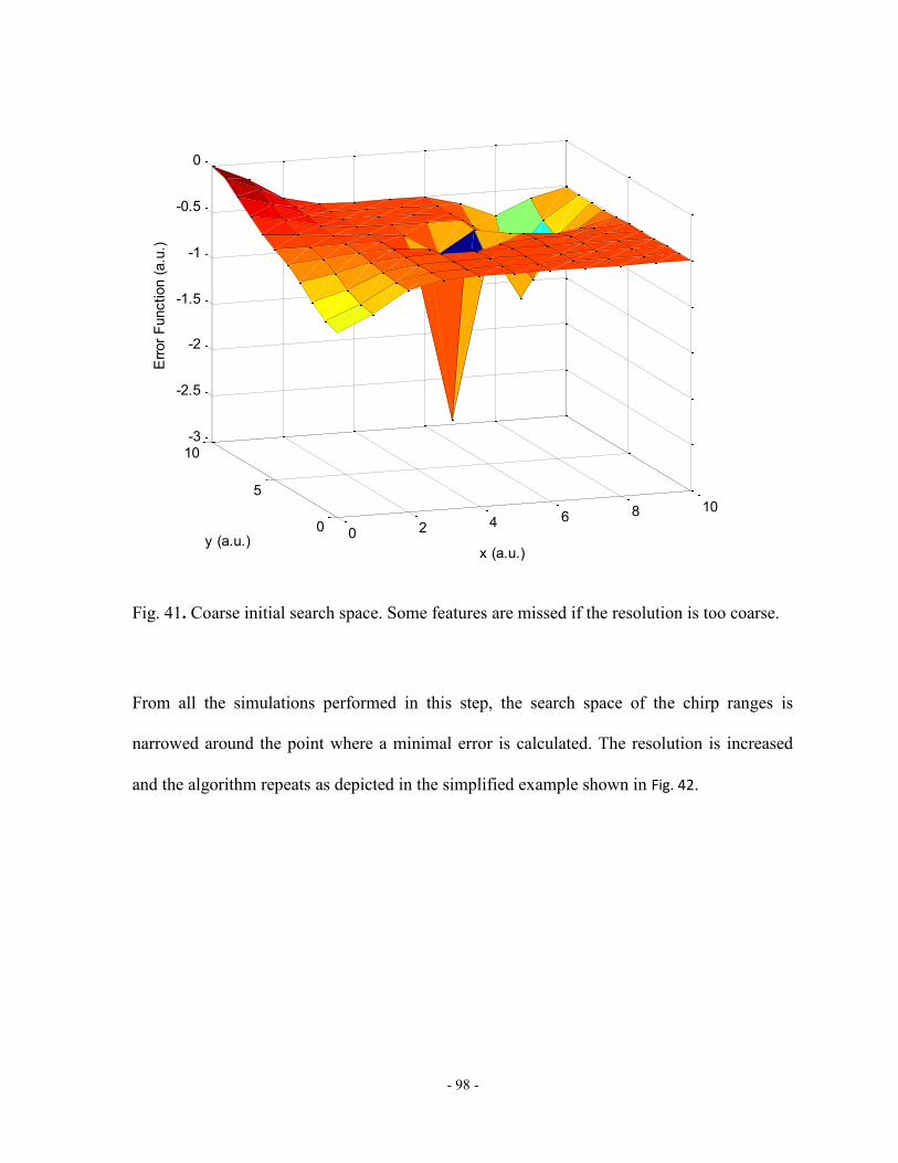
- 98 -

Fig. 41. Coarse initial search space. Some features are missed if the resolution is too coarse.

From all the simulations performed in this step, the search space of the chirp ranges is

narrowed around the point where a minimal error is calculated. The resolution is increased

and the algorithm repeats as depicted in the simplified example shown in Fig. 42.

0 2 4 6 8 10

0

5

10-3

-2.5

-2

-1.5

-1

-0.5

0

x (a.u.)y (a.u.)

Err

or

Function (

a.u

.)

- 99 -

Fig. 42. Narrowing of the search space and increased resolution.

If the point with minimal error is located on the edge of the search space, the current iteration

is re-run with the same resolution, but with a search space centered on this point. If the point

with minimal error is inside the search space, the search space in centered on this point, it is

narrowed around the minimal error point and the resolution is increased, as shown in Fig. 43.

0 2 4 6 8 10

0

5

10-3.5

-3

-2.5

-2

-1.5

-1

-0.5

0

x (a.u.)y (a.u.)

Err

or

Function (

a.u

.)

- 100 -

Fig. 43. Narrowing and centering of the search space around the minimal error point. The

resolution is further increased across all search dimensions.

The algorithm exits when a target resolution for all three chirp coefficients has been reached.

This algorithm allows runtimes to be reduced to several hours for a given target SFBG.

Fig. 44 shows the results of the simulation algorithm for a target dispersion of 500 ps/nm for

different sizes of SFBGs. The gratings are sine-square apodized, and their parameters are

shown in Table 4.

0 2 4 6 8 10

0

5

10-3.5

-3

-2.5

-2

-1.5

-1

-0.5

0

x (a.u.)y (a.u.)

Err

or

Function (

a.u

.)

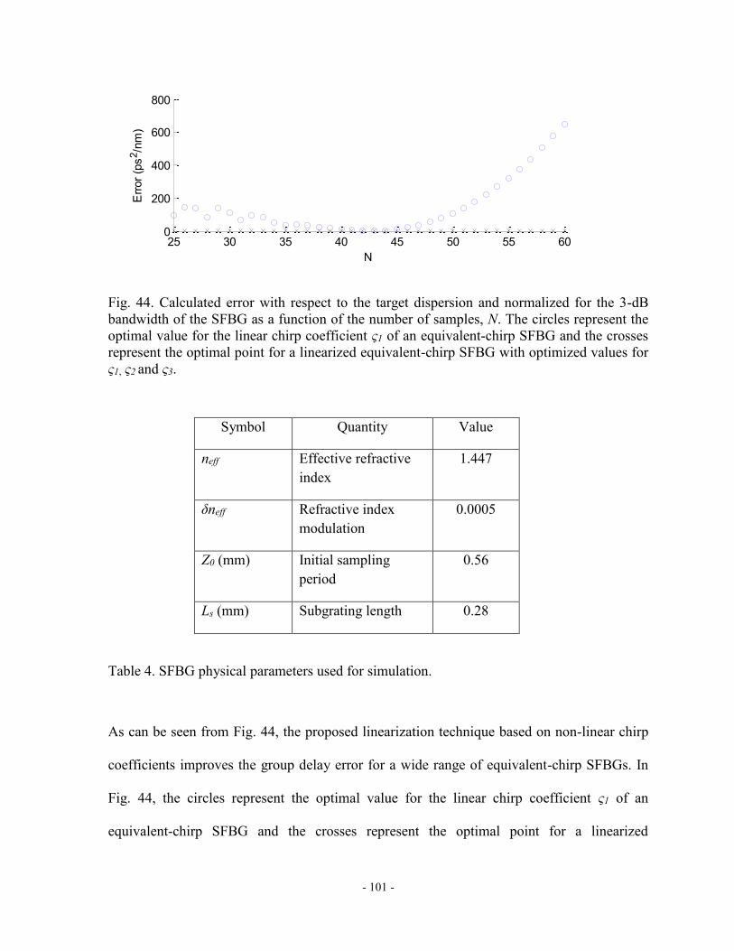
- 101 -

Fig. 44. Calculated error with respect to the target dispersion and normalized for the 3-dB

bandwidth of the SFBG as a function of the number of samples, N. The circles represent the

optimal value for the linear chirp coefficient ς1 of an equivalent-chirp SFBG and the crosses

represent the optimal point for a linearized equivalent-chirp SFBG with optimized values for

ς1, ς2 and ς3.


neff Effective refractive

index

1.447

δneff Refractive index

modulation

0.0005


period

0.56


Table 4. SFBG physical parameters used for simulation.

As can be seen from Fig. 44, the proposed linearization technique based on non-linear chirp

coefficients improves the group delay error for a wide range of equivalent-chirp SFBGs. In

Fig. 44, the circles represent the optimal value for the linear chirp coefficient ς1 of an

equivalent-chirp SFBG and the crosses represent the optimal point for a linearized

25 30 35 40 45 50 55 600

200

400

600

800

N

Err

or

(ps

2/n

m)

- 102 -

equivalent-chirp SFBG with optimized values for ς1, ς2 and ς3. When only the first-order

coefficient is used, it is still possible to realize an SFBG with a linear group delay response

with minimal error, but the number of samples contained in the SFBG has to be within a

limited range. In the example above, such an SFBG could have between 41 and 44 samples

to have a normalized group delay error of less than 10 ps2/nm for a target dispersion of 500

ps/nm. If the number of samples is too small, there is not enough resolution to properly

represent the chirp profile. On the other hand, if the number of samples is too large, the

response of the grating is very sensitive to a slight change in the non-linear chirp coefficients

and a large number of samples will lead to a significant group delay error.

With our proposed approach, the range of N giving a normalized group delay error of less

than 10 ps2/nm is between 34 and 65. By non-linearly chirping the spatial profile of the

SFBG, it is possible to compensate for the non-linearities otherwise seen in the group delay

response as shown in Fig. 38. Our proposed method gives the designer more flexibility to

choose an SFBG profile which can satisfy the group delay ripple requirements and a given

physical length, which can be a limiting factor for packaging considerations.

Fig. 45 shows that the 3-dB bandwidth of the realized SFBG varies with the number of

samples almost linearly, which can also be exploited when designing an SFBG. The fact that

the 3-dB bandwidth increases with the number of sample is explained by the chirp parameter

being a function of the z-position (which is defined along the length of the fiber). Thus,

longer gratings present a larger total chirp.

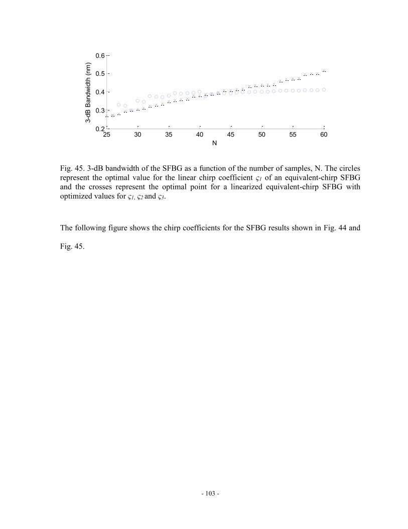
- 103 -

Fig. 45. 3-dB bandwidth of the SFBG as a function of the number of samples, N. The circles

represent the optimal value for the linear chirp coefficient ς1 of an equivalent-chirp SFBG

and the crosses represent the optimal point for a linearized equivalent-chirp SFBG with

optimized values for ς1, ς2 and ς3.

The following figure shows the chirp coefficients for the SFBG results shown in Fig. 44 and

Fig. 45.

25 30 35 40 45 50 55 600.2

0.3

0.4

0.5

0.6

N

3-d

B B

andw

idth

(nm

)

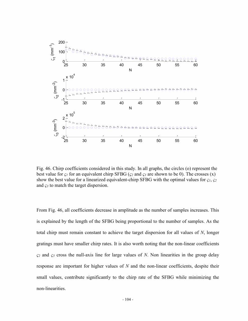
- 104 -

Fig. 46. Chirp coefficients considered in this study. In all graphs, the circles (o) represent the

best value for ς1 for an equivalent chirp SFBG (ς2 and ς3 are shown to be 0). The crosses (x)

show the best value for a linearized equivalent-chirp SFBG with the optimal values for ς1, ς2

and ς3 to match the target dispersion.

From Fig. 46, all coefficients decrease in amplitude as the number of samples increases. This

is explained by the length of the SFBG being proportional to the number of samples. As the

total chirp must remain constant to achieve the target dispersion for all values of N, longer

gratings must have smaller chirp rates. It is also worth noting that the non-linear coefficients

ς2 and ς3 cross the null-axis line for large values of N. Non linearities in the group delay

response are important for higher values of N and the non-linear coefficients, despite their

small values, contribute significantly to the chirp rate of the SFBG while minimizing the

non-linearities.

25 30 35 40 45 50 55 600

100

200

N

1 (

mm

-1)

25 30 35 40 45 50 55 60-1

0

1x 10

4

N

2 (

mm

-2)

25 30 35 40 45 50 55 60-2

0

2x 10

5

N

3 (

mm

-3)

- 105 -

The algorithm was used to improve the group delay response of the SFBG with only linear

chirp presented in Section 4.1. Table 5 shows the parameters of the SFBG simulated. The

linearization algorithm was used to find the values of ς1, ς2 and ς3. Fig. 47 (a) shows the

reflectivity, Fig. 47 (b) shows the group delay response of this improved equivalent linearly-

chirped SFBG and Fig. 47 (c) shows the group delay ripple of the simulated SFBG. The

average dispersion over the 3-dB bandwidth is 498.9 ps/nm.


N Number of samples 50


period

0.56


ς1 (mm-1) Linear-chirp

coefficient

15.486


chirp coefficient

575.8928


chirp coefficient

-7979.9107

Table 5. Parameters of an equivalent linearly-chirped SFBG with linear and non-linear chirp

coefficients.

- 106 -

(a)

(b)

1550.8 1550.9 1551 1551.1 1551.2 1551.3-10

-9

-8

-7

-6

-5

-4

-3

-2

-1

0

(nm)

Am

plitu

de

Re

sp

on

se

(d

B)

1550.8 1550.9 1551 1551.1 1551.2 1551.30

50

100

150

200

250

300

(nm)

Gro

up

De

lay R

esp

on

se

(p

s)

- 107 -

(c)

Fig. 47. Simulated spectral response of an equivalent linearly-chirped SFBG with parameters

defined in Table 3, column 4: (a) reflectivity, (b) group delay response, (c) group delay

ripple.

Fig. 47 clearly shows an improvement in the group delay response of the linearly-chirped

SFBG when non-linear chirp coefficients are used to linearize the group delay response. The

group delay ripple difference is 14.99 ps throughout the range considered. When such a

linearization technique is used, the positioning of the subgratings inside the superstructure

becomes critical. A high position precision is required to achieve high quality results. The

impact of the high-order coefficients on the subgrating position is relatively small, but these

coefficients have a high impact on the linearity of the group delay response.

1550.8 1550.9 1551 1551.1 1551.2 1551.3-20

-15

-10

-5

0

5

10

15

20

(nm)

Gro

up

De

lay R

ipp

le (

ps)

- 108 -

4.3 Fabrication of linearized equivalent-chirped SFBG

SFBGs with improved equivalent linear chirp are fabricated to validate the theory presented.

Four SFBGs are fabricated. The fabrication is implemented using a frequency-doubled

argon-ion laser operating at 244 nm with a uniform phase mask. Hydrogen-loaded

photosensitive optical fiber is used (Corning SMF-28, neff = 1.468). The gratings are

fabricated using a stepper motor to scan the laser beam along the length of the optical fiber.

Two exposures are required: the first to create the AC variation of the refractive index

profile, the second, to create the DC component of the refractive index profile. During the

first exposure, the sampling of the SFBG is done by shifting the laser beam laterally, while

closing a shutter, effectively blocking the exposure on sections of the optical fiber when the

phase mask is present. During the second exposure, the phase mask is removed and the DC

component of the refractive index profile is generated by exposing the optical fiber directly.

Table 6 shows the parameters of the gratings realized. The gratings are realized using a 14-

cm uniform phase mask. Apodization was realized by controlling the exposure time of each

sample to match that of the desired apodization profile.

- 109 -

Symbol SFBG 1 SFBG 2 SFBG 3 SFBG 4

N 20 25 30 35

Z0 (mm) 0.56 0.56 0.56 0.56

Ls (mm) 0.28 0.28 0.28 0.28

ς1 (mm-1) 117.39 117.25 100.98 92.58

ς2 (mm-2) -5337.73 -4656.25 -3361.61 -2207.58

ς3 (mm-3) 127430.33 108810.76 73604.91 38113.84

Table 6. Equivalent Linearly-Chirped SFBG Parameters

The following figures show the amplitude and phase responses of the fabricated SFBGs.

(a)

1552.55 1552.6 1552.65 1552.7-10

-8

-6

-4

-2

0

(nm)

Am

plit

ud

e R

esp

on

se

(d

B)

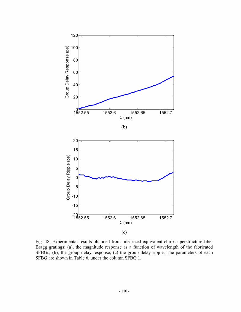
- 110 -

(b)

(c)

Fig. 48. Experimental results obtained from linearized equivalent-chirp superstructure fiber

Bragg gratings: (a), the magnitude response as a function of wavelength of the fabricated

SFBGs; (b), the group delay response; (c) the group delay ripple. The parameters of each

SFBG are shown in Table 6, under the column SFBG 1.

1552.55 1552.6 1552.65 1552.70

20

40

60

80

100

120

(nm)

Gro

up

De

lay R

esp

on

se

(p

s)

1552.55 1552.6 1552.65 1552.7-20

-15

-10

-5

0

5

10

15

20

(nm)

Gro

up

De

lay R

ipp

le (

ps)

- 111 -

(a)

(b)

1552.55 1552.6 1552.65 1552.7-10

-8

-6

-4

-2

0

(nm)

Am

plit

ud

e R

esp

on

se

(d

B)

1552.55 1552.6 1552.65 1552.70

20

40

60

80

100

120

(nm)

Gro

up

De

lay R

esp

on

se

(p

s)

- 112 -

(c)





(a)

1552.55 1552.6 1552.65 1552.7-20

-15

-10

-5

0

5

10

15

20

(nm)

Gro

up

De

lay R

ipp

le (

ps)

1552.55 1552.6 1552.65 1552.7-10

-8

-6

-4

-2

0

(nm)

Am

plit

ud

e R

esp

on

se

(d

B)

- 113 -

(b)

(c)





1552.55 1552.6 1552.65 1552.70

20

40

60

80

100

120

(nm)

Gro

up

De

lay R

esp

on

se

(p

s)

1552.55 1552.6 1552.65 1552.7-20

-15

-10

-5

0

5

10

15

20

(nm)

Gro

up

De

lay R

ipp

le (

ps)

- 114 -

(a)

(b)

1552.55 1552.6 1552.65 1552.7-10

-8

-6

-4

-2

0

(nm)

Am

plit

ud

e R

esp

on

se

(d

B)

1552.55 1552.6 1552.65 1552.70

20

40

60

80

100

120

(nm)

Gro

up

De

lay R

esp

on

se

(p

s)

- 115 -

(c)





As can be seen from Fig. 48 to Fig. 51, the group delay responses of the fabricated SFBGs

with equivalent chirps in the grating period are very close to linear and with minimal error.

To validate the theory presented, an SFBG with equivalent chirp, but without the

linearization technique applied to its spatial profile is fabricated and its characterization is

shown in Fig. 52. The deviation from a linear response is as high as 15 ps at λ = 1552.62 nm.

1552.55 1552.6 1552.65 1552.7-20

-15

-10

-5

0

5

10

15

20

(nm)

Gro

up

De

lay R

ipp

le (

ps)

- 116 -

(a)

(b)

Fig. 52. Experimental results obtained from equivalent-chirp superstructure fiber Bragg

gratings without the linearization method applied. The parameters of this SFBG are the same

as SFBG 4.

1552.55 1552.6 1552.65 1552.7-10

-8

-6

-4

-2

0

(nm)

Am

plit

ud

e R

esp

on

se

(d

B)

1552.55 1552.6 1552.65 1552.70

20

40

60

80

100

120

(nm)

Gro

up D

ela

y R

esponse (

ps)

- 117 -

With these group delay responses giving a maximal time delay progression of approximately

20 ps, it is theoretically possible to steer the main lobe of a 4-element PAA to more than

+30° and -30° from a line that is perpendicular to the array axis. The beamsteering range is

highly dependent on the geometry and the design of the PAA, in particular the antenna

element spacing. Fig. 53 shows the simulated array factors for a linear phased array antenna

fed with the true time-delay beamformer. The time delays considered are taken from the

experimental group delay responses of the superstructured fiber Bragg gratings. For

simulation purposes, s = 6.9 mm, N = 4 and fRF = 18 GHz.

(a)

0.2

0.4

0.6

0.8

1

30

210

60

240

90

270

120

300

150

330

180 0

- 118 -

(b)

(c)

0.2

0.4

0.6

0.8

1

30

210

60

240

90

270

120

300

150

330

180 0

0.2

0.4

0.6

0.8

1

30

210

60

240

90

270

120

300

150

330

180 0

- 119 -

(d)

Fig. 53. Simulated array factors for a linear phased array antenna fed with the true time-delay

beamformer. The time delays considered are taken from the experimental group delay

responses of the superstructured fiber Bragg gratings. For simulation purposes, s = 6.9 mm,

N = 4 and fRF = 18 GHz. The beam orientation is shown for (a) 90°, (b) 110°, (c) 130° and (d)

145°.

It should be noted that the usable beamsteering range is dependent on the frequency of the

microwave signal. A high frequency signal, especially when used in a double sideband

modulation scheme will occupy a large portion of the available optical bandwidth of the

SFBG prism. Designing equivalent-chirped SFBGs with a larger 3-dB bandwidth and/or

using a single sideband modulation scheme are workarounds required to address this issue.

The group delay ripples that can be observed in the group delay response plots of Fig. 48-Fig.

51 will affect the shape of the PAA’s array factor and, consequently, the orientation of the

main lobe. Fig. 54 shows the error associated with the orientation of the main lobe of the

array factor of a PAA when compared with the array factor of an ideal theoretical true time

0.2

0.4

0.6

0.8

1

30

210

60

240

90

270

120

300

150

330

180 0

- 120 -

delay progression. The error is limited to ±3.45°. It has been previously demonstrated that a

beamformer built with SFBGs, but using only a linear chirp coefficient in the design of the

SFBGs had errors in the orientation of the main lobe of the array factor of a PAA limited to

±10°. The proposed linearization of the group delay response allows a reduction in this error

by a factor of 2.9.

Fig. 54. Error in the orientation of the main lobe of the array factor as a function of the

optical carrier wavelength.

4.4 Error analysis of the designed and fabricated SFBGs

The experimental results obtained differed from the simulation results of the SFBGs with a

linearized group delay response. The cause of this error will be studied in this section.

1552.55 1552.6 1552.65 1552.7-3

-2

-1

0

1

2

3

(nm)

An

gu

lar

Err

or

( )

- 121 -

4.4.1 Simulated and experimental grating responses

The following figures show the experimental and theoretical amplitude and phase responses

of all gratings fabricated for the photonic TTD beamformer.

(a)

1552.55 1552.6 1552.65 1552.7-10

-8

-6

-4

-2

0

(nm)

Am

plit

ud

e R

esp

onse

(d

B)

- 122 -

(b)

Fig. 55. Comparison between theoretical (green, dashed line) and experimental (blue, solid

line) grating responses (a) amplitude, (b) group delay for SFBG 1.

(a)

1552.55 1552.6 1552.65 1552.70

20

40

60

80

100

120

(nm)

Gro

up

De

lay R

esp

onse

(p

s)

1552.55 1552.6 1552.65 1552.7-10

-8

-6

-4

-2

0

(nm)

Am

plit

ud

e R

esp

onse

(d

B)

- 123 -

(b)



(a)

1552.55 1552.6 1552.65 1552.70

20

40

60

80

100

120

(nm)

Gro

up

De

lay R

esp

onse

(p

s)

1552.55 1552.6 1552.65 1552.7-10

-8

-6

-4

-2

0

(nm)

Am

plit

ud

e R

esp

onse

(d

B)

- 124 -

(b)



(a)

1552.55 1552.6 1552.65 1552.70

20

40

60

80

100

120

(nm)

Gro

up

De

lay R

esp

onse

(p

s)

1552.55 1552.6 1552.65 1552.7-10

-8

-6

-4

-2

0

(nm)

Am

plit

ud

e R

esp

onse

(d

B)

- 125 -

(b)



As can be seen in Fig. 55 - Fig. 58, the amplitude and group delay response of the fabricated

SFBG differ from the theoretical model. Fabrication errors are believed to be the main source

of error for these differences. The SFBGs were characterized with a LUNA OVA 5000, an

optical vector analyzer platform. By analyzing the optical time domain response, it is

possible to deduce some sources of fabrication error and to correlate these to the errors seen

in the experimental results. The following figures show the optical time domain response of

the four SFBGs and the SFBG parameters extracted from this data.

1552.55 1552.6 1552.65 1552.70

20

40

60

80

100

120

(nm)

Gro

up

De

lay R

esp

onse

(p

s)

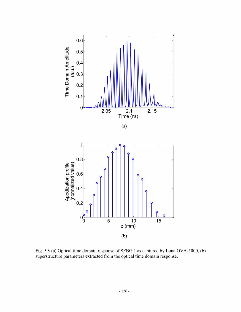
- 126 -

(a)

(b)


superstructure parameters extracted from the optical time domain response.

2.05 2.1 2.150

0.1

0.2

0.3

0.4

0.5

0.6

Time (ns)

Tim

e D

om

ain

Am

plit

ude

(a.u

.)

0 5 10 150

0.2

0.4

0.6

0.8

1

Apodiz

ation p

rofile

(norm

aliz

ed v

alu

e)

z (mm)

- 127 -

(a)

(b)



2.35 2.4 2.45 2.5 2.550

0.5

1

1.5

Time (ns)

Tim

e D

om

ain

Am

plit

ude

(a.u

.)

0 5 10 15 20 250

0.2

0.4

0.6

0.8

1

Apodiz

ation p

rofile

(norm

aliz

ed v

alu

e)

z (mm)

- 128 -

(a)

(b)



2.55 2.6 2.65 2.7 2.750

0.1

0.2

0.3

0.4

0.5

Time (ns)

Tim

e D

om

ain

Am

plit

ude

(a.u

.)

0 10 20 300

0.2

0.4

0.6

0.8

1

Apodiz

ation p

rofile

(norm

aliz

ed v

alu

e)

z (mm)

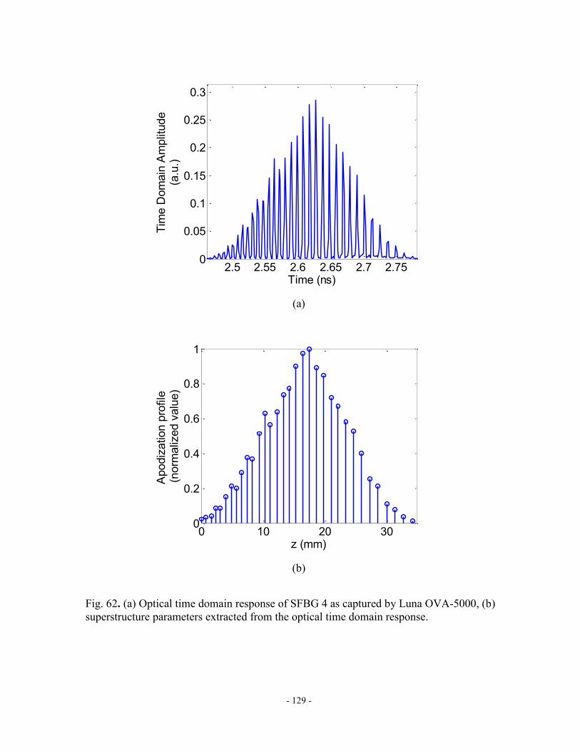
- 129 -

(a)

(b)



2.5 2.55 2.6 2.65 2.7 2.750

0.05

0.1

0.15

0.2

0.25

0.3

Time (ns)

Tim

e D

om

ain

Am

plit

ude

(a.u

.)

0 10 20 300

0.2

0.4

0.6

0.8

1

Apodiz

ation p

rofile

(norm

aliz

ed v

alu

e)

z (mm)

- 130 -

By analyzing the spacing between the time domain pulses, it is possible to deduce the sample

function of the fabricated SFBG. Furthermore, the relative apodization profile of the

superstructure can be determined by the amplitude of each time domain pulse. By extracting

these values, and comparing them to the theoretical model, we can better appreciate the

impact of any difference on the SFBG amplitude and group delay response.

(a)

1552.55 1552.6 1552.65 1552.7-10

-8

-6

-4

-2

0

(nm)

Am

plit

ud

e R

esp

onse

(d

B)

- 131 -

(b)

Fig. 63. Comparison of a simulated SFBG response (green, dashed line) with experimental

results (blue, solid line) for SFBG 1. The superstructure parameters of the simulated SFBG

are extracted from the optical time domain response: (a) Amplitude response, (b) Group

delay response.

(a)

1552.55 1552.6 1552.65 1552.70

20

40

60

80

100

120

(nm)

Gro

up

De

lay R

esp

onse

(p

s)

1552.55 1552.6 1552.65 1552.7-10

-8

-6

-4

-2

0

(nm)

Am

plit

ud

e R

esp

onse

(d

B)

- 132 -

(b)




delay response.

(a)

1552.55 1552.6 1552.65 1552.70

20

40

60

80

100

120

(nm)

Gro

up

De

lay R

esp

onse

(p

s)

1552.55 1552.6 1552.65 1552.7-10

-8

-6

-4

-2

0

(nm)

Am

plit

ud

e R

esp

onse

(d

B)

- 133 -

(b)




delay response.

(a)

1552.55 1552.6 1552.65 1552.70

20

40

60

80

100

120

(nm)

Gro

up

De

lay R

esp

onse

(p

s)

1552.55 1552.6 1552.65 1552.7-10

-8

-6

-4

-2

0

(nm)

Am

plit

ud

e R

esp

onse

(d

B)

- 134 -

(b)




delay response.

From Fig. 63 to Fig. 66, we can observe that the amplitude and group delay responses

simulated based on superstructure parameters extracted from the optical time domain

response are closer to the experimental results measured by the Luna OVA. This would

indicate that a good portion of the error is attributable to fabrication errors in the amplitude of

the refractive index modulation inside the subgratings, as well as errors in the physical

location of the subgratings. While the optical time domain response provides some insight on

some aspects of the superstructures, notably the sampling function and the apodization of the

superstructure, some uncertainty remains on the apodization profile of the subgratings and

the effective refractive index inside the blank spaces. This may explain the remaining error

between the experimental SFBG response and the theoretical simulation of the grating.

1552.55 1552.6 1552.65 1552.70

20

40

60

80

100

120

(nm)

Gro

up

De

lay R

esp

onse

(p

s)

- 135 -

4.5 Summary

We have proposed and demonstrated a technique to improve the linearity of the group delay

response of an SFBG with an equivalent chirp. Four SFBGs designed based on the proposed

technique were fabricated. The experimental results were well in agreement with the theory

presented and errors could be attributed to uncertainties with the fabrication process, which

were also reflected in a spatial refractive index profile mismatch. An error analysis was

carried out and SFBG were simulated based on physical parameters of the superstructure

extracted from the optical time domain response.

When designing an SFBG with an equivalent chirp, one must take care in selecting the

number of sampling periods to match the target dispersion is only a linear chirp coefficient is

used. With our technique, we expand the number of possible values that will yield an

acceptable group delay response, giving the possibility to fabricate physically shorter

gratings or gratings with tailored 3-dB bandwidths to meet the requirements for a particular

application. Furthermore, the group delay responses of the fabricated SFBGs offer a

reduction by a factor of 2.9 in the error associated with the orientation of the main lobe of the

array factor of a PAA when compared to the experimental results reported in Section 3.2.

- 136 -

OPTICAL SINGLE SIDEBAND MODULATION USING AN ULTRA-

NARROW DUAL-TRANSMISSION-BAND FIBER BRAGG GRATING

In order to make use of the SFBG TTD beamformer presented in the previous chapters, a

SSB modulation scheme is required as the optical bandwidth of the SFBG is limited.

Many efforts have been invested in finding ways to combat the chromatic-dispersion-induced

power penalty that occurs when optical signal that has been DSB+C modulated by an RF

carrier propagates through standard single mode fiber (SMF) [36]-[39]. The power penalty is

caused by the beating of both sidebands with the optical carrier upon being detected at a PD.

This beating generates two RF signals, one for each sideband. The relative phase difference

between both signals leads to a power penalty, should the signals be out of phase. The use of

SSB modulation can eliminate completely the chromatic-dispersion-induced power penalty

as only one sideband is being transmitted and thus, only one RF signal is generated by the

beating of this sideband with the optical carrier at the PD.

Several approaches have been proposed to implement SSB modulation for radio-over-fiber

(RoF) systems. The use of narrowband filters such as regular FBGs [36], [37] to attenuate

one of the two sidebands has been reported. Since regular FBGs have relatively broad

bandwidth, for RoF system operating at a few GHz, such as at 2.4 GH or 5.8 GHz, it is hard

to only remove one sideband without affecting the optical carrier and the other sideband.

Another technique using a dual-electrode Mach-Zehnder modulator (MZM) [38] does not

have this problem, but the configuration requires an electrical phase shifter to introduce a π/2

phase shift in the RF signal. Optical SSB modulation scheme can also be implemented based

on stimulated Brillouin scattering (SBS) [39], but the approach is only suitable for a RoF

system operating at 11-GHz.

- 137 -

5.1 SSB modulator based on equivalent phase shift in SFBG

In this section, we present a novel approach to realizing optical SSB modulation by using an

ultra-narrow dual-transmission-band equivalent phase shift (EPS) SFBG. In the proposed

system, a DSB+C modulated optical signal is sent to the input of an optical SSB filter. This

filter, based on an EPS SFBG, serves as a dual-transmission-band filter and is used to

transmit one sideband with the optical carrier, thus achieving optical SSB. SFBGs with

equivalent phase shifts can produce ultra-narrow transmission bands [81]-[84]. The use of

equivalent phase shifts reduces significantly the accuracy required from the FBG fabrication

system. In this experiment, an EPS SFBG with two equivalent phase shifts is fabricated. The

use of EPS SFBG to implement the SSB modulation is demonstrated and the influence of the

EPS SFBG on the bit error rate performance is studied.

It has been shown that by extending the period of specific sections in the SFBG, it is possible

to create equivalent phase shifts as

ZZZm extPS /2 , (65)

where θPS corresponds to the angle of the phase shift and Zext is the period of the extended

section.

From (65), it is possible to achieve a π-phase shift in the ±1-order channels by extending a

period by 50%.

In order to create two peaks in the transmission spectrum of an SFBG, two equivalent π-

phase shifts must be created. This can be realized by extending the lengths of two sections by

- 138 -

50%. In this work, a 40-section SFBG that has a duty cycle of 0.5 and with the 18th and the

22nd sections extended by 50% is fabricated to create two equivalent π-phase shifts. The

length of the subgratings is kept constant for all sections in the structure. The transmission

spectrum of the superstructure presents two transmission peaks separated by 0.09 nm, which

corresponds to 11.24 GHz in the 1550-nm region. Fig. 67 shows a diagram of the fabricated

superstructure FBG.

1 2 3 18 22 38 39 40

Z 1.5 Z 1.5 Z

...

... ...

......

Fig. 67. Schematic diagram of the superstructure FBG for SSB generation.

The SSB filter proposed is composed of a SFBG used as a transmission grating and a

uniform FBG used in reflection. The spectrum of the uniform FBG used in reflection should

be complementary to that of the superstructure grating, with the exception of the two

transmission peaks, as shown in Fig. 68. By aligning a sideband and the optical carrier with

the two transmission peaks, it is possible to suppress the other sideband, leading to the

generation of an SSB signal. Furthermore, the proposed filter allows the suppression of

higher order sidebands as the uniform FBG used in reflection attenuates sidebands that would

otherwise pass through with the SFBG alone.

- 139 -

EPS SFBG

Optical Spectrum

TransmissionSpectrum

Optical Spectrum

FBG

ReflectionSpectrum

Optical Spectrum

Propagation direction

Fig. 68. Configuration of the SSB filter based on a superstructure FBG with two equivalent

phase shifts.

5.2 Experimental results

The transmission spectrum of the realized SSB filter based on a SFBG is shown in Fig. 69(a).

A theoretical spectrum is also shown for comparison purposes. As it can be seen, the

experimental and the theoretical spectra coincide well, which confirms the theoretical model

presented.

The spacing of the two transmission peaks of the superstructure grating is measured to be

0.09 nm. This corresponds to a frequency of 11.2 GHz in the 1550-nm region. Based on this

value, an apodized uniform FBG is designed and fabricated. The passband of the reflection

filter has to be large enough to allow the reflection of both the optical carrier and one

sideband without significant attenuation and narrow enough to filter the other sideband. Fig.

69(b) shows the reflection spectrum of the fabricated uniform FBG. The 3 dB bandwidth is

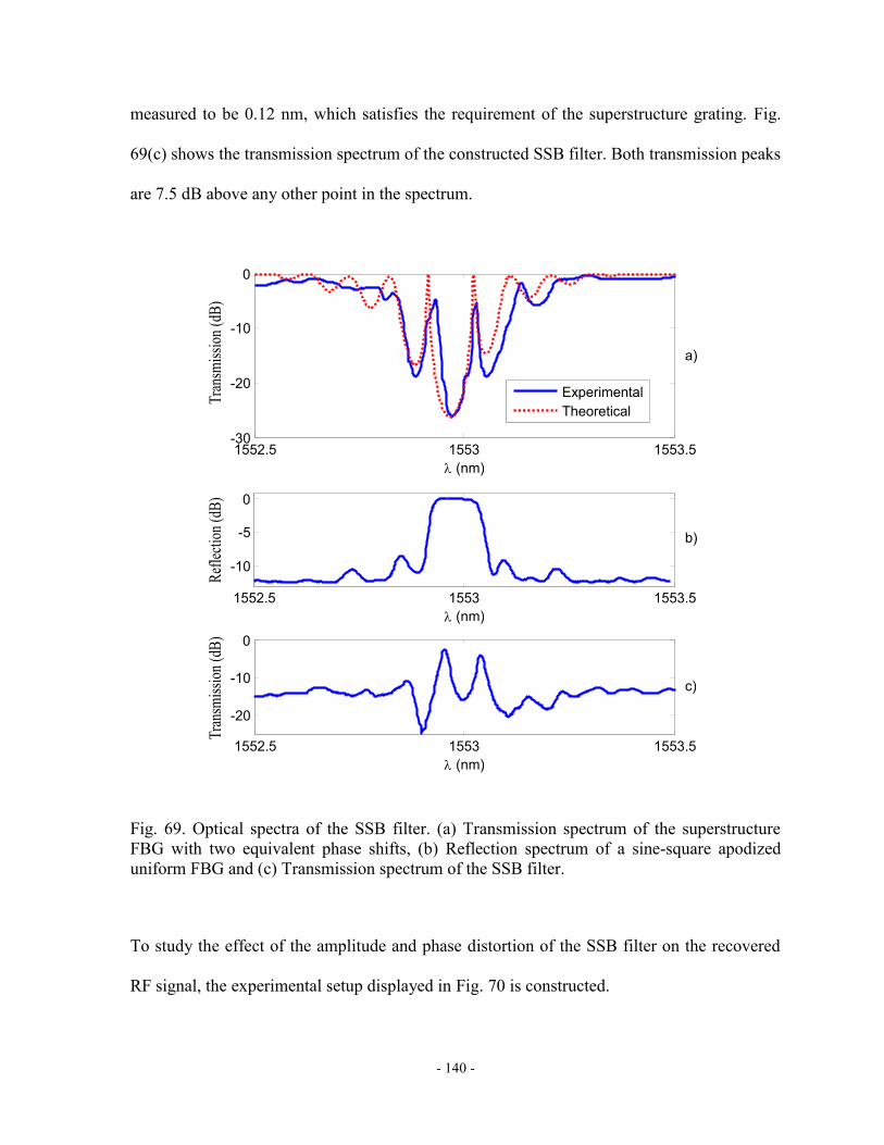
- 140 -

measured to be 0.12 nm, which satisfies the requirement of the superstructure grating. Fig.

69(c) shows the transmission spectrum of the constructed SSB filter. Both transmission peaks

are 7.5 dB above any other point in the spectrum.

Fig. 69. Optical spectra of the SSB filter. (a) Transmission spectrum of the superstructure

FBG with two equivalent phase shifts, (b) Reflection spectrum of a sine-square apodized

uniform FBG and (c) Transmission spectrum of the SSB filter.

To study the effect of the amplitude and phase distortion of the SSB filter on the recovered

RF signal, the experimental setup displayed in Fig. 70 is constructed.

1552.5 1553 1553.5

-30

-20

-10

0

(nm)

1552.5 1553 1553.5

-10

-5

0

(nm)

1552.5 1553 1553.5

-20

-10

0

(nm)

Experimental

Theoretical

a)

b)

c)

- 141 -

TLS PC EOM SSB Filter EDFA

PD

Amp

Mixer

Amp

3 dB

Coupler

Signal

Generator OscilloscopeData

Generator

Mixer

Amp

Fig. 70. Schematic diagram of the SSB generation system: TLS: tunable laser source; PC:

polarization controller; EOM: electro-optic modulator; EDFA: Erbium-doped fiber amplifier;

PD: photodetector.

In the electrical domain, an NRZ, 100 Mb/s pseudo-random bit sequence with a word length

of 223-1 is generated by a bit error rate (BER) tester. This data stream is frequency-up-

converted at 11 GHz via a mixer before being amplified. An optical carrier is modulated via

an electro-optic modulator (EOM) by this electrical signal. A polarization controller (PC) is

used to minimize the polarization-dependent loss associated with the EOM. To achieve SSB

modulation in the optical domain, the modulated optical signal is sent to the SSB filter. The

spectrum of the optical signal after the SSB filter is presented in Fig. 71. The lower-

sideband-to-upper-sideband ratio is equal to 23.1 dB. The electrical signal is recovered via a

photodetector (PD) and is amplified. A second mixer is used for frequency down-conversion

- 142 -

to recover the 100 Mb/s bit sequence before amplifying it and sending it to the oscilloscope

or to the bit error rate tester.

Fig. 71. Spectrum of the SSB modulated optical signal at the output of the SFBG filter.

Fig. 72 (a) and (b) show the eye diagrams of the electrical signal transmitted using optical

SSB modulation and optical DSB+C modulation, respectively. The signal has been slightly

distorted by the SSB filter, especially at the rising and falling edges, but the eye diagram is

still very open.

1552.5 1553 1553.5

-60

-40

-20

(nm)

Optical P

ow

er

(dB

m)

- 143 -

(a)

(b)

Fig. 72. (a) Eye diagram of the electrical signal transmitted using optical SSB modulation

and recovered; (b) Eye diagram of the electrical signal transmitted using optical DSB+C

modulation and recovered.

- 144 -

Fig. 73 shows the BER curves (back-to-back) of the recovered electrical signal. The power

penalty for the SSB modulation, which is attributable to the distortion and the power loss

caused by the SSB filter, is 2.5 dB.

Fig. 73. BER power penalty caused by the SSB filter.

5.3 Evaluation of dispersion effects on the recovered electrical signal

5.3.1 Double sideband modulation

In the proposed system, an optical carrier is intensity modulated (IM) by an external electro-

optic modulator. Electro-optic modulators, as their name states, are based on the electro-optic

effect, i.e., the modification of the refractive index of a nonlinear crystal by an electric field.

The modification of the refractive index is proportional to the electric field strength. [90]-

-20 -19 -18 -17 -16 -15 -14-12-11-10

-9-8

-7

-6

-5

-4

-3

Received Optical Power (dBm)

log

(BE

R)

SSB

DSB

- 145 -

[92].

Non-centrosymmetric crystal materials exhibit a linear relation between the electric field

strength and the refractive index change. This electro-optic effect is also called Pockels

effect. Other transparent media exhibit the Kerr electro-optic effect, where the refractive

index change is proportional to the square of the electric field strength. This effect is

typically much weaker than the Pockels effect. Materials exhibiting the Pockels effect are

called electro-optic materials.

The refractive index change of an electro-optic material is given by

2

3EnrEn

,

(66)

where r is the electro-optic effect coefficient, n is the effective refractive index of the

medium and E is the strength of the electrical field applied to the crystal.

By varying the strength of the electric field, the phase of the optical signal passing through

the crystal will be changed. This phase variation will be directly proportional to the strength

of the electric field and phase modulation of the optical carrier is obtained. The total phase

change over an interaction length Lmod is given by

mod2 Ln ,

(67)

where λ is the free space wavelength of the optical signal.

In order to achieve an intensity modulation scheme, this phase modulator is used in a Mach-

Zehnder interferometer. Fig. 74 illustrates the configuration used.

- 146 -

Fig. 74. Mach-Zehnder based electro-optic modulator.

By using (67), it is possible to find the phase shift in the upper branch as a function of the

electric field strength

mod22 LEnLn

Eupper

upper , (68)

where Lupper is the total length of the upper branch of the interferometer, Lmod is the length of

the Pockels cell, δn(E) is the refractive index change caused by the electric field as described

in (66) and λ is the free space wavelength of the optical signal.

Similarly, the phase shift of the upper branch of the interferometer is given by

lower

lower

Ln2 ,

(69)

where Llower is the length of the lower branch of the interferometer.

- 147 -

If the waveguide divides the input optical power equally, the output optical intensity is

related to the input intensity by the well-known interferometer equation

2cos 2

tItI inout,

(70)

where is the phase difference between the two branches of the interferometer defined as

lowerupper . (71)

When the phase difference is being controlled with a linear relation for a Pockels effect, the

transmittance of the electro-optic modulator becomes a function of the applied voltage as

V

VVT

22cos mod2

mod , (72)

where

lowerupper LLn

2, Vmod is the applied voltage and Vπ is the voltage to achieve a

π phase shift between the beams of the two arms of the interferometer. In order to produce a

linear intensity modulator, the optical path difference has to be adjusted so that 2

. When

this is the case, (70) can be approximated as

tVm

tItI i

inout mod1

2 ,

(73)

where Vmod(t) is the electric signal applied to the Mach-Zehnder modulator and mi is the

modulation index depth.

The optical intensity is proportional to the square of the amplitude of the optical electrical

field. If Vmod(t) is expressed as

- 148 -

ttV RFcosmod . (74)

The output optical electrical field of the modulator, Emod(t), can be expressed as

cctj

cRFi eEtmtE

cos1mod,

(75)

where ωRF is the modulating angular frequency of the RF signal, Ec, ωc, and c are the

amplitude of the input optical electrical field, the optical carrier angular frequency, and the

initial phase of the optical carrier, respectively.

If we expand the mathematical expression of the amplitude of this intensity modulated signal

into its Fourier series, we get

0

coscos1i

RFiRFRFiRF tiKEtmE , (76)

where

T

RFi dttmT

K0

0 cos11

, (77)

and

T

RFRFin dttitmT

K0

coscos12

(78)

for i = 1, 2, 3, …

When mi is small, the Fourier series can be approximated as

2

1

1

0

imK

K

(79)

- 149 -

and the higher order coefficients can be considered negligible. Under these conditions, when

higher order harmonics can be neglected, the intensity modulated optical signal can be

approximated by an amplitude modulated signal [93] as

cc tj

cRFa eEtmtE

cos1mod,

(80)

where ma is the normalized amplitude modulation index.

It is well known that the Fourier transform of an amplitude modulated signal is given by

C

CC

j

RFCC

a

j

RFCC

aj

Cc

eEm

eEm

eEE

2

2mod

(81)

From this equation, three frequency components are present at ωc, ωc + ωRF and ωc – ωRF.

The first component is located at the carrier frequency and the two remaining components are

the upper and lower sidebands respectively. This modulation type is also referred to as

double sideband (DSB) modulation.

5.3.2 Single sideband modulation

In the case where one of the sidebands is suppressed, the modulation is then referred to as

single sideband modulation. Single sideband modulation in the optical domain can be

achieved by using a dual electrode Mach-Zehnder modulator [94] [96] with a hybrid coupler

providing a π/2 phase shift difference between the microwave electrical signals applied to the

electrodes. Another amplitude modulation scheme can be created by amplitude modulating

the microwave signal. The double sideband modulated optical signal is then filtered in the

- 150 -

optical domain such that only one of the sidebands is suppressed by the filter [94] [97].

Bragg gratings can be used for filtering the unwanted sideband. In this case, (81) can be

expressed as either

cc j

RFcc

aj

cc eEm

eEE

2mod

(82)

or

cc j

RFcc

aj

cc eEm

eEE

2mod .

(83)

From these equations, two frequency components are present at ωc and ωc + ωRF or at ωc and

ωc - ωRF. The first component is located at the carrier frequency and the remaining

component is the single sideband.

5.3.3 Dispersion effects of a single mode fiber

A modulated optical signal propagating through an optical fiber of significant length will

suffer from chromatic dispersion. When the frequency components of this modulated optical

signal are recovered by a photodetector, the difference between the phases of each

component may introduce a power penalty depending on the modulation scheme used [38],

[98]-[102]. The dispersion and group delay for a standard single mode fiber are given

respectively by [103]

4

00 14

SD

(84)

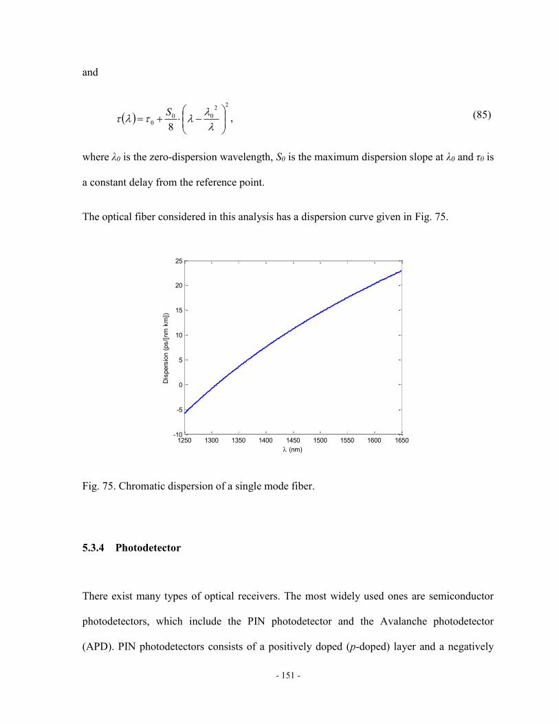
- 151 -

and

2

2

000

8

S, (85)

where λ0 is the zero-dispersion wavelength, S0 is the maximum dispersion slope at λ0 and τ0 is

a constant delay from the reference point.

The optical fiber considered in this analysis has a dispersion curve given in Fig. 75.

Fig. 75. Chromatic dispersion of a single mode fiber.

5.3.4 Photodetector

There exist many types of optical receivers. The most widely used ones are semiconductor

photodetectors, which include the PIN photodetector and the Avalanche photodetector

(APD). PIN photodetectors consists of a positively doped (p-doped) layer and a negatively

1250 1300 1350 1400 1450 1500 1550 1600 1650-10

-5

0

5

10

15

20

25

Dis

pers

ion (

ps/[

nm

km

])

(nm)

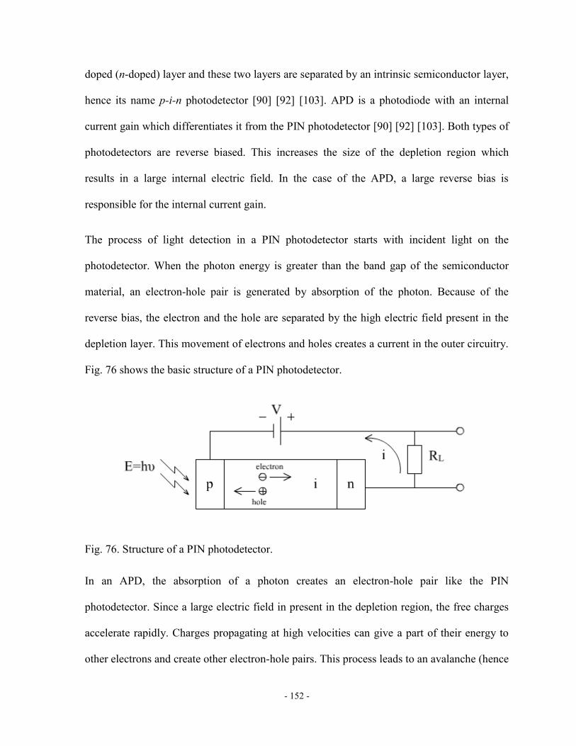
- 152 -

doped (n-doped) layer and these two layers are separated by an intrinsic semiconductor layer,

hence its name p-i-n photodetector [90] [92] [103]. APD is a photodiode with an internal

current gain which differentiates it from the PIN photodetector [90] [92] [103]. Both types of

photodetectors are reverse biased. This increases the size of the depletion region which

results in a large internal electric field. In the case of the APD, a large reverse bias is

responsible for the internal current gain.

The process of light detection in a PIN photodetector starts with incident light on the

photodetector. When the photon energy is greater than the band gap of the semiconductor

material, an electron-hole pair is generated by absorption of the photon. Because of the

reverse bias, the electron and the hole are separated by the high electric field present in the

depletion layer. This movement of electrons and holes creates a current in the outer circuitry.

Fig. 76 shows the basic structure of a PIN photodetector.

Fig. 76. Structure of a PIN photodetector.

In an APD, the absorption of a photon creates an electron-hole pair like the PIN

photodetector. Since a large electric field in present in the depletion region, the free charges

accelerate rapidly. Charges propagating at high velocities can give a part of their energy to

other electrons and create other electron-hole pairs. This process leads to an avalanche (hence

- 153 -

the name of the photodetector) multiplication of the charges. Fig. 77 illustrates the structure

of an APD.

Fig. 77. Structure of an avalanche photodetector.

The relation between the incident optical power Po and the photocurrent Ip for both PIN

photodetectors and APDs is given by

0Ph

qMI p

, (86)

where M is the multiplication factor of the APD and is equal to 1 for a PIN photodiode, η is

the quantum efficiency, q is the electron charge and h ν is the photon energy.

The quantum efficiency which can be calculated as

0P

I

q

h p . (87)

Another important parameter is the responsitivity of the photodetector given by

- 154 -

h

q

P

I p

0

. (88)

This last parameter is quite useful in practice as it gives the photocurrent generated per unit

optical power.

5.3.5 Recovered microwave signal by a photodetector

A) Double sideband modulation

In the case of a remotely controlled phased array antenna, the intensity modulated optical

signal reaching the photodetector is given by

URFcU

a

LRFcL

a

cccPD

tEm

tEm

tEtE

cos2

cos2

cos

(89)

where θc, θL, θU, ρc, ρL, ρU represent the phase shifts caused by both the reflectivity of the

Bragg grating and by the chromatic dispersion of the single mode fiber and the amplitude

reflection introduced by the Bragg grating for all three frequency components: the optical

carrier, the lower sideband and the upper sideband, respectively.

When considering only frequencies centered on ωRF of the recovered microwave signal, we

get

cUm

Uca

Lcm

Lca tEm

tEm

ty

cos2

cos2

22

. (90)

Considering the following identity,

- 155 -

21

2112

22

21

coscos

sinsinarctancoscos2

coscos

BA

BAtBABA

tBtA

, (91)

we can express (90) as

cUULcL

cUULcL

RF

cULULULca

t

Emty

coscos

sinsinarctancos

2cos2222

. (92)

B) Single sideband modulation

In the case of a remotely controlled phased array antenna, the SSB modulated optical signal

reaching the photodetector, considering that the upper sideband is kept is given by

URFcU

a

cccPD tEm

tEtE cos2

cos , (93)

where θc, θU, ρc, ρU represent the phase shifts caused by both the reflectivity of the Bragg

grating and by the chromatic dispersion of the single mode fiber and the amplitude reflection

introduced by the Bragg grating for both frequency components, the optical carrier and the

upper sideband.

When considering only frequencies centered on ωRF of the recovered microwave signal, we

get

)cos()( 2

UcRFUca tmEty . (94)

- 156 -

5.3.6 Impact on system performance

Considering (92) and (94), it is possible to conclude that the DSB modulation format will

affect the amplitude of the signal recovered at the PD as long as

cLU 2 . (95)

When propagating through a length of SMF, it can be approximated that the amplitude of the

sidebands and the optical carrier will not be affected significantly. The following

approximation can be made:

ULc .

(96)

With the approximation given in (96), it is possible to simplify (92) as

2cos

2cos

22 LU

RFc

LU

ca tEmty

. (97)

The amplitude of the power at the output of the PIN photodiode at the frequency fRF is given

approximately by [104]-[106]

c

fLDP RF

fel

222

, cos

. (98)

In the case of an 11.2 GHz electrical carrier frequency, an important power penalty occurs at

specific lengths, the first notch being at

222 RFfD

cL

, (99)

- 157 -

which, for the parameters considered, corresponds to a length of SMF of 29.3 km. Fig. 78

shows the power penalty as a function of the length of SFM for a microwave frequency of

11.2 GHz.

Fig. 78. Power penalty of a DSB modulation scheme with a microwave frequency of 11.2

GHz as a function of SMF length.

5.4 Summary

A novel SSB filter based on a superstructure FBG with two equivalent phase shifts was

constructed. Two ultra-narrow transmission bands in the superstructure FBG, separated by

11.2 GHz, allow the selection of the optical carrier and of one sideband to generate an optical

SSB signal. The spectrum of a uniform FBG used in reflection should be complementary to

that of the superstructure grating, with the exception of the two transmission peaks. This

0 10 20 30 40 50 60 70 80 90 100-70

-60

-50

-40

-30

-20

-10

0

SMF length (km)

Pow

er

Penalty (

dB

)

- 158 -

FBG is required to further attenuate the unwanted sideband which falls partly outside of the

stop band of the SFBG. The experimental optical SSB signal realized shows a lower-

sideband-to-upper-sideband ratio of 23.1 dB. It was experimentally demonstrated that the

back-to-back BER power penalty caused by the SSB filter is 2.5 dB for a 100 Mb/s pseudo-

random bit sequence. This approach is thus well suited for the transmission of data up to 100

Mb/s and requires a frequency up-conversion at 11 GHz.

- 159 -

ALL-OPTICAL BANDPASS MICROWAVE FILTER BASED ON A

SUPERSTRUCTURED FIBER BRAGG GRATING WITH EQUIVALENT

CHIRP

All-optical microwave filters have been studied extensively in the past few years [40]-[48].

They are meant to offer the same functionalities than their electrical counterparts, but to

provide many advantages such as: low loss, high bandwidth, immunity to electromagnetic

interference (EMI) and, very importantly, tunability, which is often hard to achieve at high

frequencies for microwave filters implemented using electronic circuits.

Fiber delay line signal processing has been first proposed by Wilner and Van den Heuvel

[107] who noted the high available bandwidth and the low loss of optical fibers as suitable

for processing broadband signals.

In the optical domain, photonic microwave filters are designed to operate in the incoherent

regime to avoid optical interference which is very sensitive to environmental changes.

Incoherent photonic microwave filters usually have all positive coefficients. It is known that

an all-positive-coefficient microwave delay-line filter functions as a low-pass filter only.

6.1 All-optical bandpass microwave filter

Recently, several approaches have been proposed to address the issue of photonic microwave

filters with only positive coefficients. We demonstrate a two-tap all-optical bandpass

microwave filter with one negative coefficient. The negative coefficient is generated based

- 160 -

on optical phase modulation to intensity modulation (PM-IM) conversion in a chirped fiber

Bragg grating (CFBG). The CFBG is a superstructured FBG with an equivalent chirp. The

experimental setup is discussed, followed by experimental results. The tunability of the free

spectral range of the microwave filter is achieved by adjusting the wavelength of the optical

carrier.

The all-optical bandpass microwave filter demonstrated uses a PM-IM conversion to

generate a negative coefficient. The phase modulation is realized using an electro-optic phase

modulator (EOPM), and the PM-IM conversion is achieved using a dispersive device [47]-

[48]. It is well known that the spectrum of a phase modulated optical signal, under small

signal approximation, consists of three frequency components: an optical carrier and two

sidebands. At the output of the EOPM, the upper and lower sidebands are exactly out of

phase. Upon detection by a fast photodetector, the beating of the lower sideband with the

optical carrier will generate an electrical signal which has a π-phase shift with the electrical

signal generated by the beating of the upper sideband and the optical carrier. The two

generated electrical signals thus cancel each other, leaving only a DC component (which is

usually filtered out by a DC blocker).

6.2 PM-IM conversion

The idea behind PM-IM conversion is to change the phase relationship between the two

sidebands with respect to the optical carrier. By propagating through a dispersive medium,

the three main frequency components of a phase-modulated optical signal will experience

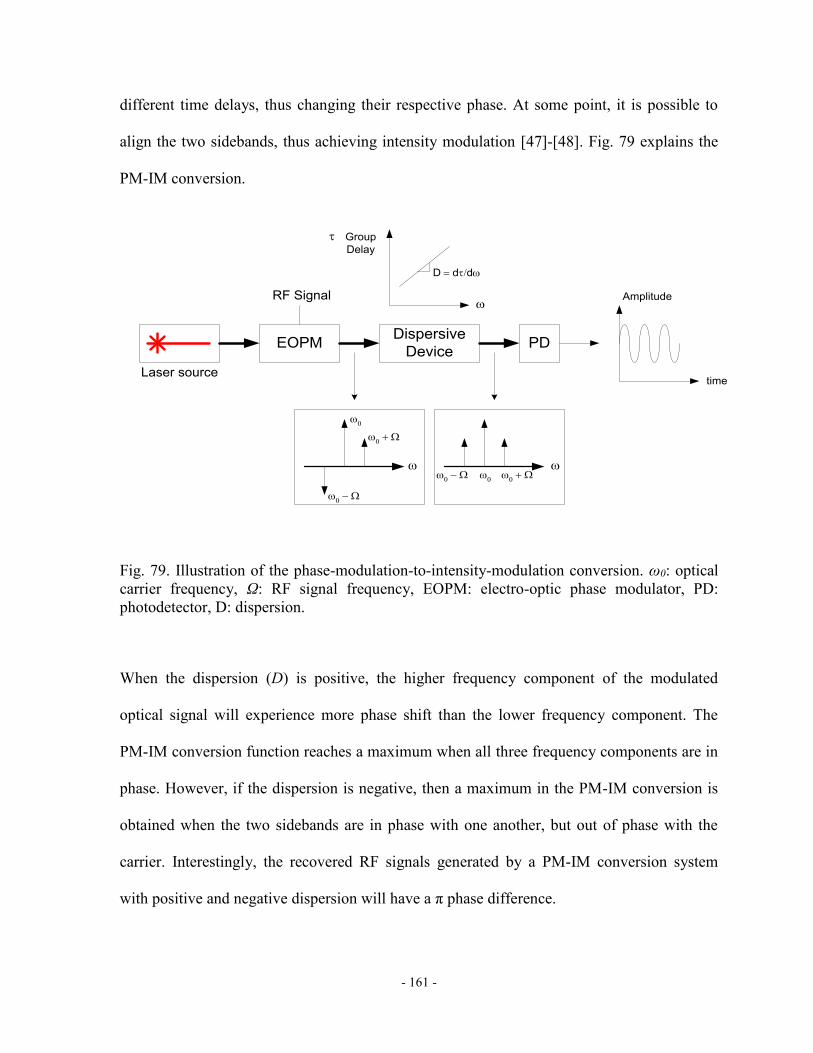
- 161 -

different time delays, thus changing their respective phase. At some point, it is possible to

align the two sidebands, thus achieving intensity modulation [47]-[48]. Fig. 79 explains the

PM-IM conversion.

EOPMDispersive

DevicePD

Group

Delay

Laser source

RF Signal

time

Amplitude

Ddd

Fig. 79. Illustration of the phase-modulation-to-intensity-modulation conversion. ω0: optical

carrier frequency, Ω: RF signal frequency, EOPM: electro-optic phase modulator, PD:

photodetector, D: dispersion.

When the dispersion (D) is positive, the higher frequency component of the modulated

optical signal will experience more phase shift than the lower frequency component. The

PM-IM conversion function reaches a maximum when all three frequency components are in

phase. However, if the dispersion is negative, then a maximum in the PM-IM conversion is

obtained when the two sidebands are in phase with one another, but out of phase with the

carrier. Interestingly, the recovered RF signals generated by a PM-IM conversion system

with positive and negative dispersion will have a π phase difference.

- 162 -

In the microwave filter realized, this property is exploited to implement a filter with positive

and negative coefficients. For a two-tap filter, two laser diodes (LDs) are used to generate

two optical carriers at different wavelengths, which are phase-modulated by an electro-optic

phase modulator (EOPM) after being combined by an optical combiner. The phase-

modulated optical signals are sent to an arrayed waveguide grating (AWG) to separate each

signal before sending them to the SFBGs. Because of the chromatic dispersion of each

SFBG, the reflected signal is converted from phase modulation to intensity modulation. The

reflected optical signals are recombined by the AWG and sent to a photodetector (PD) to

recover the filtered modulating RF signal. The gain of each tap can be adjusted by changing

the power of the appropriate LD. The delay progression increases linearly for all the taps by

controlling the delay line lengths.

6.3 All-optical bandpass microwave filter configuration

As mentioned, SFBGs with equivalent chirp are used as the dispersive devices for the PM-

IM conversion. In order to achieve different dispersion of opposite signs, the SFBGs can be

connected to their opposite ports. In the case where two taps have the same gain amplitude,

but with a different sign, the same SFBG can be used for both taps, provided that the

bandwidth of the SFBG is large enough to accommodate the two wavelengths associated

with the taps.

The main advantage of using SFBGs for the realization of such filters lies in the fabrication

process simplicity and flexibility. Conventionally, to achieve chirped FBGs with different

- 163 -

chirp rates, phase masks tailored for each FBG response must be used. For SFBGs, a single

uniform phase mask is used. The dispersion of an equivalent-chirp SFBG can be controlled

by carefully designing the sampling function of the SFBG during the fabrication process.

Fig. 80 shows the configuration of the all-optical bandpass microwave filter based on

equivalent-chirp SFBGs.

LD 1

LD 2

Optical

CombinerEOPM

PD

RF Signal

Filtered RF Signal

SFBG 1

SFBG 2

l1

l1 + l

Fig. 80. All-optical bandpass microwave filter configuration based on equivalent-chirp

superstructured fiber Bragg gratings (SFBG). LD: laser diode, EOPM: electro-optic phase

modulator, PD: photodetector.

The transfer function of the proposed filter configuration is given by

2

1

12

2sin

n

njnn e

DPH ,

(100)

where Pn is the optical power of the nth LD, Dn is the dispersion of the nth equivalent chirp

SFBG, Ω is the RF signal frequency and Δτ is the time delay difference between each branch,

caused by the length difference between the two optical paths, Δl and is given by

- 164 -

c

lneff

2 ,

(101)

where neff is the refractive index of the optical fiber and c is the speed of light in vacuum (~ 3

× 108 m/s).

A two-tap all-optical microwave filter based on a single SFBG is demonstrated. In the

proposed configuration, a loop structure is employed, which enables the implementation of a

two-tap filter with a single LD and a single equivalent-chirp SFBG. The experimental setup

is shown in Fig. 81.

LD EOPM

PD

SFBG

l1

l1 + l

PC

Isolator 3 dB

Vector Network Analyser

Fig. 81. Experimental setup of the proposed all-optical microwave filter based on an SFBG.

LD: laser diode, PC: polarization controller, EOPM: electro-optic phase modulator, 3 dB:

50/50 optical coupler, SFBG: superstructured fiber Bragg grating, PD: photodetector.

An RF signal is generated by a vector network analyzer (VNA) and is used to phase-

modulate an optical carrier. The modulated optical signal is split into two with a 3-dB

coupler. Each signal travels through different lengths of optical fiber before reaching the

equivalent-chirp SFBG. Both signals are reflected and converted to intensity modulation

because of the dispersion value of the SFBG. Because both sides of a single SFBG are used,

the two dispersion values are of opposite sign. Thus, one tap is positive and the other is

- 165 -

negative. The reflected and dispersed optical signals are recombined via the 3-dB coupler and

send to a photodetector (PD). An optical isolator is used to block counter-propagating light

from reaching the EOPM and the LD.

The reflection spectrum of the fabricated SFBG and its group delay response are shown in

Fig. 82(a). The SFBG is fabricated on hydrogen loaded fiber with the following

superstructure parameters: Z0 = 1 mm, Ls = 0.8 mm, N = 50, ς1 = 0.014247, ς2 = 0. A

theoretical reflection spectrum is also shown in Fig. 82(b) for comparison purposes. As it can

be seen, the experimental and the theoretical spectra have similar responses. Uncertainties in

several parameters, including the duty cycle of the superstructure grating and the modulation

depth of the refractive index may be the cause of any discrepancies.

(a)

1552.2 1552.25 1552.3 1552.35 1552.4 1552.45-30

-26

-22

-18

-14

-10

-6

-2

2

(nm)

Re

fle

ctivity (

dB

)

0

100

200

300

400

500

600

700

800

Gro

up

De

lay (

ps)

- 166 -

(b)

Fig. 82. (a) Measured reflection spectrum and group delay of the realized equivalent-chirp

superstructured fiber Bragg grating, (b) theoretical reflectivity and group delay response of

the superstructured fiber Bragg grating.

The fabricated SFBG has a dispersion value of χ = 2100 ps/nm, which gives the first peak

and the first notch of the PM-IM conversion located at 5.45 GHz and 7.70 GHz, respectively.

This corresponds well with the experimental response of the PM-IM conversion using the

SFBG, which is shown in Fig. 83.

1552.2 1552.25 1552.3 1552.35 1552.4 1552.45-30

-26

-22

-18

-14

-10

-6

-2

2

(nm)

Re

fle

ctivity (

dB

)

0

100

200

300

400

500

600

700

800

Gro

up D

ela

y (

ps)

- 167 -

Fig. 83. Experimental response of the phase-modulation-to-intensity-modulation conversion

using an equivalent-chirp superstructured fiber Bragg grating with a dispersion value of 2100

ps/nm.

In the realized microwave filter, a time-delay difference of 350 ps is measured between the

two taps. This corresponds to a path length difference of 3.6 cm. The FSR of the filter is thus

2.86 GHz. Again, this value matches well the measured response of the realized microwave

filter, as shown in Fig. 84.

0 1 2 3 4 5 6 7 8 9 10-35

-30

-25

-20

-15

-10

-5

0

Frequency (GHz)

No

rma

lize

d fre

qu

en

cy r

esp

on

se

(d

B)

- 168 -

Fig. 84. Experimental response of the implemented filter with one positive and one negative

coefficient.

As it can be seen from (100), the overall response of the filter is the multiplication of the PM-

IM conversion by a 2-tap (one negative and one positive) filter response with a given FSR.

This can be clearly seen in Fig. 83 and Fig. 84. The notch at 7.7 GHz is present in the filter

response, as is the peak at 5.45 GHz.

6.4 Summary

The results presented in this section show that the experimental implementation of a

microwave filter based on an SFBG matches closely the theoretical model presented. Firstly,

a 50-section equivalent-chirp SFBG with a chirp parameter ς1 = 0.014247 has been fabricated

and tested. The reflectivity and the group delay response of the SFBG follow the theoretical

0 1 2 3 4 5 6 7 8 9 10-40

-35

-30

-25

-20

-15

-10

-5

0

Frequency (GHz)

No

rma

lize

d fre

qu

en

cy r

esp

on

se

(d

B)

- 169 -

model. As the fabricated SFBG is fairly long (72.2 mm), the fabrication process is very

sensitive to small alignment errors. This can explain the differences between the theoretical

model and the fabricated SFBG.

The PM-IM conversion has been properly characterized based on the dispersion value of the

SFBG. The FSR of the filter has been calculated based on the optical path length difference.

The calculated value of 2.86 GHz matches closely the response of the filter, which shows an

FSR of around 2.92 GHz. The use of PM-IM conversion allows the creation of a microwave

filter with negative coefficients. A bandpass filter, which is only realizable with negative

coefficients, has been implemented for the first time using an SFBG with equivalent chirp in

the sampling period.

- 170 -

CONCLUSION AND FUTURE WORK

7.1 Conclusions

The main objective of this thesis was to investigate the utilization of SFBG in various

microwave photonics application, notable those related with true time-delay beamforming

systems for phased array antennas.

CHAPTER 2 presented the theory associated with Bragg gratings based on the coupled-mode

theory was also introduced and simulation results of Bragg gratings. The concept of

superstructured fiber Bragg gratings was also presented and simulation methods for both

types of gratings were presented. The notions of equivalent phase shifts in SFBGs and of

equivalent chirp were discussed and examples of grating responses for each type of SFBGs

were shown. In the same chapter, the theoretical models of phased array antennas were

presented and the main equations characterizing these antennas were developed. The notions

of true time delay and phase shifting were presented and the obvious advantages of the true

time-delay method were listed.

CHAPTER 3 presented a photonic true-time delay beamforming system for phased array

antennas based on SFBGs with linearly increasing equivalent chirps. A theoretical analysis of

the influence of errors in the group delay response on the array factor was detailed.

Experimental spectra and group delay responses of the SFBGs have been presented. The

error in the angle of the main lobe of the array factor was calculated based on the

experimental group delay values and was limited to ±10° over the entire band of operation.

- 171 -

CHAPTER 4 presented the technique proposed to achieve linear group delay responses with

minimal deviations and errors from a perfect slope in SFBGs with equivalent chirp in their

sampling profiles. Experimental results of fabricated SFBG with the optimized linear and

non-linear chirp coefficients were presented and the simulation algorithm developed to find

the optical chirp coefficients has been detailed.

CHAPTER 5 presented a novel method to achieve a SSB modulation scheme that employs an

SFBG with two equivalent phase shifts in its sampling profile. Two ultra-narrow

transmission bands in the SFBG, separated by 11.2 GHz, allowed the selection of the optical

carrier and of one sideband to generate an optical SSB signal. The experimental optical SSB

signal realized showed a lower-sideband-to-upper-sideband ratio of 23.1 dB.

CHAPTER 6 proposed a new way to implement an all-optical bandpass microwave filter

with an SFBG with an equivalent chirp in its sampling period. To construct the filter, a 50-

section equivalent-chirp SFBG with a chirp parameter ς1 = 0.014247 was fabricated and

tested. The reflectivity and the group delay response of the SFBG followed the theoretical

model and deviations from the theoretical model can be attributed to small optical alignment

errors during the SFBG fabrication process. The PM-IM conversion has been characterized

and the FSR of the filter has been calculated based on the optical path length difference. The

calculated value of 2.86 GHz matches closely the response of the filter, which shows an FSR

of around 2.92 GHz. The use of PM-IM conversion allows the creation of a microwave filter

with negative coefficients. A bandpass filter, which is only realizable with negative

coefficients, has been demonstrated experimentally.

- 172 -

7.2 Future work

SFBGs offer a lot of potential for use in microwave photonics applications. Novel ways to

shape their spectral responses provide a great appeal for more research in this area in order to

find new applications for the gratings and to find new properties of the superstructure

profiles.

During the investigation on achieving a linear group delay response for SFBG with

equivalent chirp in their sampling profile, it was discovered that not all gratings parameters

can yield good results to achieve a target dispersion. For example, it is inconceivable that a

grating with only two sections could yield a linear group delay response regardless of the

value of the linear and non-linear chirp coefficients. More research should be made to better

understand the limitations of SFBG with equivalent chirps in order to guide a designer into

choosing the optimal grating parameters for a given application based on its requirements.

Also, the 3-dB bandwidth of the SFBG is often narrow for applications where a high

frequency RF signal is modulated onto an optical carrier. This essentially limits the steering

capability of the beamformer based on SFBGs and this may also limit the operating

microwave bandwidth of a photonic microwave filter. A better understanding of the effects

of grating and superstructure parameters of an SFBG on the 3-dB bandwidth of its +/-1st

orders would be beneficial for these reasons.

- 173 -

BIBLIOGRAPHY

[1] K. O. Hill, Y. Fujii, D. C. Johnson, B. S. Kawasaki, “Photosensitivity in optical

fiber waveguides: application to reflection fiber fabrication,” Appl. Phys. Lett.,

vol. 32, no. 10, pp. 647-649, 1978.

[2] G. Meltz, W. W. Morey, and W. H. Glenn, "Formation of Bragg gratings in

optical fibers by a transverse holographic method," Opt. Lett., vol. 14, no. 15, pp.

823-825, 1989.

[3] X.-F. Chen, X.-H. Li, L. Xia, S.-Z. Xie, C.-C. Fan and J.-P. Want, “Experimental

investigation of a sampled grating with a chirp in the sampling period,” Microw.

Opt. Technol. Lett., vol. 29, no. 2, pp. 128-130, Apr. 2001.

[4] S.R. Blais and J.Yao, “Photonic true-time delay beamforming based on

superstructured fiber Bragg gratings with linearly increasing equivalent chirps,” J.

Lightw. Technol., vol. 27, no. 9, pp. 1147-1154, 2009.

[5] S.R. Blais and J. Yao, “Tunable photonic microwave filter using a superstructured

FBG with two reflection bands having complementary chirps,” IEEE Photon.

Technol. Lett., vol. 20, no. 3, pp. 199-201, Feb. 2008.

[6] J.S. Leng, W. Zhang and J.A.R. Williams, “Optimization of superstructured fiber

Bragg gratings for microwave photonic filters response,” IEEE Photon. Technol.

Lett., vol. 16, no. 7, pp. 1736-1738, Jul. 2004.

[7] D. Jiang, X. Chen, Y. Dai, H. Liu and S. Xie, “A novel distributed feedback fiber

laser based on equivalent phase shift,” IEEE Photon. Technol. Lett., vol. 16, no.

12, pp. 2598-2600, 2004.

- 174 -

[8] X. Chen, Y. Luo, C. C. Fan, T. Wu and S. Xie, “Analytical expression of sampled

Bragg gratings with chirp in the sampling period and its application in dispersion

management design in a WDM system,” IEEE Photon. Technol. Lett., vol. 12, no.

8, pp. 1013-1015, 2000.

[9] L. Xia, P. Shum, and C. Lu, “Flexible chirp control using the linearly inherent

chirped phase mask with the equivalent chirp design,” Opt. Comm., vol. 261, no.

1, pp. 56-59, 2006.

[10] Y. Dai, X. Chen, D. Jiang, S. Xie, C. Fan, “Equivalent phase shift in a fiber Bragg

grating achieved by changing the sampling period,” IEEE Photon. Technol. Lett.,

vol. 16, no. 10, pp. 2284-2286, 2004.

[11] S.R. Blais and J.Yao, “Photonic true-time delay beamforming based on

superstructured fiber Bragg gratings with linearly increasing equivalent chirps,” J.

Lightw. Technol., vol. 27, no. 9, pp. 1147-1154, 2009.

[12] O. Raz, R. Rotman, Y Danziger, and M. Tur, “Implementation of photonic true

time delay using high-order-mode dispersion compensating fibers,” IEEE Photon.

Technol. Lett., vol. 16, no. 5, pp. 1367-1369, May 2004.

[13] D. Dolfi, D. Mongardien, S. Tonda, M. Schaller, and J. Chazelas, “Photonics for

airborne phased array radars,” IEEE Int. Conf. Phased Array Syst. Technol., pp.

379-382, May 2000.

[14] R. A. Minasian and K. E. Alameh, “Optical-fiber grating-based beamforming

network for microwave phased arrays,” IEEE Trans. Microwave Theory Tech.,

vol. 45, no. 8, pp. 1513-1517, Aug. 1997.

- 175 -

[15] L. Xu, R. Taylor, and S. R. Forrest, “The use of optically coherent detection

techniques for true-time delay phased array and systems,” J. Lightw. Technol.,

vol. 13, no. 8, pp. 1663-1678, Aug. 1995.

[16] Y. Chen and R. T. Chen, “A fully packaged true time delay module for a K-band

phased array antenna system demonstration,” IEEE Photon. Technol. Lett., vol.

14, no. 8, pp. 1175-1177, Aug. 2002.

[17] D. N. McQuiddy, Jr., R. L. Gassner, P. Hull, J. S. Mason, and J.M. Bedinger,

“Transmit/receive module technology for X-band active array radar,” Proceedings

of the IEEE, vol. 79, no. 3, pp. 308-341, Mar. 1991.

[18] R. Rotman, O. Raz, and M. Tur, “Requirements for true time delay imaging

systems with photonic components,” IEEE Int. Symp. Phased Array Syst.

Technol., pp. 193-198, Oct. 2003.

[19] P. M. Freitag and S. R. Forrest, “A coherent optically controlled phased array

antenna system,” IEEE Microw. Guided Wave Lett., vol. 3, no. 9, pp. 293-295,

Sept. 1993.

[20] W. Ng, A. A. Walston, G. L. Tangonan, J. J. Lee, I. L. Newberg, and N.

Bernstein, “The first demonstration of an optically steered microwave phased

array antenna using true-time-delay,” J. Lightw. Technol., vol. 9, no. 9, pp. 1124-

1131, Sept. 1991.

[21] K.-L. Deng, K.I. Kang, I. Glask, and P. Prucnal, “A 1024-channel fast tunable

delay line for ultrafast all-optical TDM networks,” IEEE Photon. Technol. Lett.,

vol. 9, no. 11, pp. 1496-1498, 1997.

- 176 -

[22] D.A. Henderson, C. Hoffman, R. Culhane, and D. Viggiano III, “Kilohertz

scanning, all-fiber optical delay line using piezoelectric actuation,” Proceedings

of SPIE, vol. 5589, no. 14, pp. 99-106, Oct. 2004.

[23] R.A. Soref, "Fiber grating prism for true time delay beamsteering,” Fiber

Integrated Optics, vol. 15, no. 4, pp. 325–333, 1996.

[24] H. Zmuda, R.A. Soref, P. Payson, S. Johns, E.N. Toughlian, “Photonic

beamformer for phased array antennas using a fiber grating prism,” IEEE Photon.

Technol. Lett., vol. 9, no. 2, pp. 241-243, 1997

[25] Y. Liu, J. Yao, J. Yang, “Wideband true-time-delay unit for phased array

beamforming using discrete-chirped fiber grating prism,” Opt. Comm., vol. 2vol.

207, pp. 177-187, 2002.

[26] J.L. Cruz, B. Ortega, M.V. Andrés, B. Gimeno, D. Pastor, J. Capmany, L. Dong,

“Chirped fibre Bragg gratings for phased-array antennas,” Electron. Lett., vol. 33,

no. 7, pp. 545-546, 1997.

[27] A. Molony, “Fiber Bragg-grating true time-delay systems: discrete-grating array

3-b delay lines and chirped-grating 6-b delay lines,” IEEE Trans. Microw. Theor.

Tech., vol. 45, no. 8, pp. 1527-1530, 1997.

[28] B. Zhou, X. Zheng, X. Yu, H. Zhang, Y. Guo, B. Zhou, “Impact of group delay

ripples of chirped fiber grating on optical beamforming networks,” Optic.

Express, vol. 16, no. 4, pp. 2398-2404, 2008.

[29] D.B. Hunter, M.E. Parker, J.L. Dexter, “Demonstration of a continuously variable

true-time delay beamformer using a multichannel chirped fiber grating,” IEEE

Trans. Microw. Theor. Tech., vol. 54, no. 2, pp. 861-867, 2006.

- 177 -

[30] Y. Liu, J. Yao, J. Yang, “Wideband true-time-delay beam former that employs a

tunable chirped fiber grating prism,” Appl. Optic., vol. 42, no. 13, pp. 2273-2277,

2003.

[31] J.L. Corral, J. Marti, S. Regidor, J.M.Foster, R. Laming, M.J. Cole, “Continuously

variable true time-delay optical feeder for phased-array antenna employing

chirped fiber grating,” IEEE Trans. Microw. Theor. Tech., vol. 45, no. 8, pp.

1531-1536, 1997.

[32] Y. Liu, J. Yang, J. Yao, “Continuous true-time-delay beamforming for phased

array antenna using a tunable chirped fiber grating delay line,” IEEE Photon.

Technol. Lett., vol. 14, no. 8, pp. 1172-1174, 2002.

[33] M.Y. Frankel, “Fiber-optic true time steering of an ultrawide-band receive array,”

IEEE Trans. Microw. Theor. Tech., vol. 45, no. 8, pp. 1522-1526, 1997.

[34] M.V. Drummond, P.P. Monteiro, R.N. Nogueira, “Photonic true-time delay

beamforming based on polarization-domain interferometers,” J. Lightwave Tech.,

vol. 2vol. 28, no. 17, pp. 2492-2498, 2010.

[35] R. C. Hansen, “Phased array antennas,” John Wiley & Sons, Inc., New York,

USA, 1998.

[36] J. Park, W. V. Sorin and K. Y. Lau, “Elimination of the fibre chromatic dispersion

penalty on 1550 nm millimetre-wave optical transmission,” Electron. Lett., vol.

33, no. 6, pp. 512-513, 1997.

[37] M. Attygalle, C. Lim, G. J. Pendock, A. Nirmalathas, G. Edvell, “Transmission

improvement in fiber wireless links using fiber Bragg gratings,” IEEE Photon.


- 178 -

[38] G. H. Smith, D. Novak, Z. Ahmed, “Overcoming chromatic-dispersion effects in

fiber-wireless systems incorporating external modulators,” IEEE Trans. Microw.

Theor. Tech., vol. 45, no. 8, pp. 1410-1415, 1997.

[39] Y. Shen, X. Zhang, K. Chen, “Optical single sideband modulation of 11-GHz RoF

system using stimulated brillouin scattering,” IEEE Photon. Technol. Lett., vol.

17, no. 6, pp. 1277-1279, 2005.

[40] S. Sales, J. Capmany, J. Marti and D. Pastor, “Experimental demonstration of

fibre-optic delay line filters with negative coefficients,” Electron. Lett., vol. 31,

no. 13, pp. 1095-1096, 1995.

[41] F. Coppinger, S. Yegnanarayanan, P.D. Trinh and B. Jalali, “All-optical RF filter

using amplitude inversion in a semiconductor optical amplifier,” IEEE Trans.

Microw. Theor. Tech., vol. 48, no. 8, pp. 1473-1477, 1997.

[42] X. Wang and K.T. Chan, “Tunable all-optical incoherent bipolar delay-line filter

using injection-locked Fabry-Perot laser and fibre Bragg gratings,” Electron.

Lett., vol. 36, no. 24, pp. 2001-2003, 2000.

[43] L. Shenping, K.S. Chiang, A. Gambling, Y. Liu, L. Zhang and I. Bennion, “A

novel tunable all-optical incoherent negative-tap fiber-optic transversal filter

based on a DFB laser diode and fiber Bragg gratings,” IEEE Photon. Technol.

Lett., vol. 12, no. 9, pp. 1207-1209, 2000.

[44] J. Capmany, D. Pastor, A. Martinez, B. Ortega and S. Sales, “Microwave

photonic filters with negative coefficients based on phase inversion in an electro-

optic modulator,” Opt. Lett., vol. 2vol. 28, no. 16, pp. 1415-1417, 2003.

- 179 -

[45] E.H.W. Chan and R.A. Minasian, “Novel all-optical RF notch filters with

equivalent negative tap response,” IEEE Photon. Technol. Lett., vol. 16, no. 5, pp.

1370-1372, 2004.

[46] J. Mora, M.V. Andrés, J.L. Cruz, B. Ortega, J. Capmany, D. Pastor and S. Sales,

“Tunable all-optical negative multitap microwave filters based on uniform fiber

Bragg gratings,” Opt. Lett., vol. 2vol. 28, no. 5, pp. 1308-1310, 2003.

[47] F. Zeng and J.P. Yao, “All-optical bandpass microwave filter based on an electro-

optic phase modulator,” Opt Expr., vol. 12, no. 16, pp. 3814-3819, 2004.

[48] F. Zeng, J. Wang and J.P. Yao, “All-optical microwave bandpass filter with

negative coefficients based on a phase modulator and linearly chirped fiber Bragg

gratings,” Opt. Lett., vol. 30, no. 17, pp. 2203-2205, 2005.

[49] K.O. Hill and G. Meltz, “Fiber Bragg grating technology fundamentals and

overview,” J. Lightwave Tech., vol. 15, no. 8, pp. 1263-1276, Aug. 1997.

[50] B.S. Kawasaki, K.O. Hill, D.C. Johnson, and Y. Fujii, “Narrow-band Bragg

reflectors in optical fibers,” Opt. Lett., vol. 3, no. 2, pp. 66-68, Aug. 1978.

[51] K.O. Hill, Y. Fujii, D.C. Johnson, and B.S. Kawasaki, “Photosensitivity in optical

fiber waveguides: application to reflection fiber fabrication,” Appl. Phys. Lett.,

vol. 32, no. 10, pp. 647-649, May 1978.

[52] G. Meltz, W.W. Morey, and W.H. Glenn, “Formation of Bragg gratings in optical

fibers by a transverse holographic method,” Opt. Lett., vol. 14, no. 15, pp. 823-

825, Aug. 1989.

[53] R. Kashyap, "Fiber Bragg gratings," Academic Press, California, USA, 1999.

- 180 -

[54] M. McCall, “On the application of coupled mode theory for modeling fiber Bragg

gratings,” J. Lightwave Tech., vol. 18, no. 2, pp. 236-242, Feb. 2000.

[55] T. Erdogan, “Fiber grating spectra,” J. Lightwave Tech., vol. 15, no. 8, pp. 1277-

1294, Aug. 1997.

[56] A. Carballar and M.A. Muriel, “Phase reconstruction from reflectivity in fiber

Bragg gratings,” J. Lightwave Tech., vol. 15, no. 8, pp. 1314-1322, Aug. 1997.

[57] A. Yariv, “Coupled-mode theory for guided-wave optics,” IEEE J. Quant.

Electron., vol. QE-9, no. 9, Sept. 1973.

[58] H.G. Fröhlich and R. Kashyap, “Two methods of apodisation of fibre-Bragg-

gratings,” Opt. Comm., vol. 157, no. 1-6, pp. 273-281, Dec. 1998.

[59] R. Kashyap, A. Swanton, and D.J. Armes, “Simple technique for apodising

chirped and unchirped fibre Bragg gratings,” Electron. Lett., vol. 32, no. 13, pp.

1226-1228, Jun. 1996.

[60] J. Albert, K.O. Hill, B. Malo, S. Theriault, F. Bilodeau, D.C. Johnson, and L.E.

Erickson, “Apodisation of the spectral response of fibre Bragg gratings using a

phase mask with variable diffraction efficiency,” Electron. Lett., vol. 31, no. 3,

pp. 222-223, Feb. 1995.

[61] B. Malo, S. Thériault, D.C. Johnson, F. Bilodeau, J. Albert, and K.O. Hill,

“Apodised in-fibre Bragg grating reflectors photoimprinted using a phase mask,”

Electron. Lett., vol. 31, no. 3, pp. 223-225, Feb. 1995.

[62] M. Matsuhara and K.O. Hill, “Optical-waveguide band-rejection filters: design,”

Appl. Opt., vol. 13, no. 12, pp. 2886-2888, Dec. 1974.

- 181 -

[63] K.O. Hill, “Aperiodic distributed-parameter waveguides for integrated optics,”

Appl. Opt., vol. 13, no. 8, pp. 1853-1856, Aug. 1974.

[64] P. Fernandez, F. Alonso, J.C. Aguado, I. de Miguel, F. Gonzalez, J. Blas, J.

Duran, R. Lorenzo, E. Abril, and M. Lopez, “Simulation and design tool for

spectral characterization of fiber Bragg gratings,” Proc. 4th Int. Conf. Transparent

Optical Networks, vol. 2vol. 2, pp. 57-60, Apr. 2002.

[65] J. Ciosmak and M. Marciniak, “Impact of apodisation on fiber Bragg grating

reflection and phase responses,” Proc. 3rd Int. Conf. Transparent Optical

Networks, pp. 287-290, Jun. 2001.

[66] S.J. Mihailov, F. Bilodeau, K.O. Hill, D.C. Johnson, J. Albert, and A.S. Holmes,

“Apodization technique for fiber grating fabrication with a halftone transmission

amplitude mask,” Appl. Opt., vol. 39, no. 21, pp. 3670-3677, Jul. 2000.

[67] M. Matsuhara and K.O. Hill, “Optical-waveguide band-rejection filters: design,”

Appl. Opt., vol. 13, no. 12, pp. 2886–2888, Dec. 1974.

[68] K.O. Hill, F. Bilodeau, B. Malo, T. Kitagawa, S. Thériault, D.C. Johnson, J.

Albert, and K. Takiguchi, “Chirped in-fiber Bragg gratings for compensation of

optical-fiber dispersion,” Opt. Lett., vol. 19, no. 17, pp. 1314–1316, Sept. 1994.

[69] L. Wang, F.-P. Yan, Y.-F. Li, T.-R. Gong, and S.-S. Jian, “Impact of apodisation

functions on group delay and reflectivity ripple of chirped fiber Bragg gratings,”

Optoelectron. Lett., vol. 2vol. 2, no. 6, pp. 430-432, Nov. 2006.

[70] V. Mizrahi and J.E. Sipe, “Optical properties of photosensitive fiber phase

gratings,” J. Lightwave Tech., vol. 11, no. 10, pp. 1513-1517, 1993.

- 182 -

[71] J. Capmany, M.A. Muriel, S. Sales, J.J. Rubio, and D. Pastor, “Microwave V-I

transmission matrix formalism for the analysis of photonic circuits: application to

fiber Bragg gratings,” J. Lightwave Tech., vol. 21, no. 12, pp. 3125-3134, Dec.

2003.

[72] P.D. Lungu, “Transfer matrix method used for numerical simulation of the Bragg

reflector at perpendicular incidence of the incident field,” 1995 International

Semiconductor Conference CAS’95, pp. 613-616, Oct. 1995.

[73] M. Yamada and K. Sakuda, “Analysis of almost-periodic distributed feedback

slab waveguide via a fundamental matrix approach,” Appl. Opt., vol. 26, no. 16,

pp. 3474-3478, 1987.

[74] F. Bilodeau, B. Malo, J. Albert, D.C. Jonson, and K.O. Hill, “Photosensitization

of optical fiber and silica-on-silicon/silica waveguides,” Opt. Lett., vol. 18, no.

12, pp. 953-955, Jun. 1993.

[75] S.J. Mihailov, C.W. Smelser, D. Grobnic, R.B. Walker, P. Lu, H. Ding, and J.

Unruh, “Bragg gratings written in all-SiO/sub 2/ and Ge-doped core fibers with

800-nm femtosecond radiation and a phase mask,” J. Lightwave Tech., vol. 2vol.

22, no. 1, pp. 94-100, Jan. 2004.

[76] K.O. Hill, B. Malo, F. Bilodeau, D.C. Johnson, and J. Albert, “Bragg gratings

fabricated in monomode photosensitive optical fiber by UV exposure through a

phase mask,” Appl. Phys. Lett., vol. 62, no. 10, pp. 1035-1037, Mar. 1993.

[77] J. Canning and M.G. Skeats, “π-Phase shifted periodic distributed structures in

optical fibers by UV post-processing,” Electron. Lett., vol. 30, no. 16, pp. 1244-

1245, Aug. 1994.

- 183 -

[78] V. Jayaraman, D.A. Cohen, and L.A. Coldren, “Demonstration of broadband

tunability of a semiconductor laser using sampled gratings,” Appl. Phys. Lett.,

vol. 60, no. 19, pp. 2321-2323, May 1992.

[79] B.J. Eggleton, P.A. Krug, L. Poladin, and F. Ouellette, “Long periodic

superstructure Bragg gratings in optical fibres,” Electron. Lett., vol. 30, no. 19,

pp. 1620-1621, Sept. 1994.

[80] R.C. Hansen, “Phased array antennas,” John Wiley & Sons, Inc., New York,

USA, 1998.

[81] X. Chen, Z. Deng, and J.P. Yao, “Photonic generation of microwave signal using

a dual-wavelength single-longitudinal-mode fiber ring laser,” IEEE Trans.

Microwave Theory Tech., vol. 54, no. 2, pp. 804-809, 2006.

[82] X. Chen, J.P. Yao, F. Zeng, and Z. Deng, “Single-longitudinal-mode fiber ring

laser employing an equivalent phase-shifted fiber Bragg grating,” IEEE Photon.


[83] X. Chen, J.P. Yao, and Z. Deng, “Ultranarrow dual-transmission-band fiber Bragg

grating filter and its application in a dual-wavelength single-longitudinal-mode

fiber ring laser,” Opt. Lett., vol. 30, no. 16, pp. 2068-2070, 2005.

[84] Y. Dai, X. Chen, D. Jiang, S. Xie and C. Fan, “Equivalent phase shift in a fiber

Bragg brating achieved by changing the sampling period,” IEEE Photon. Technol.

Lett., vol. 16, no. 10, pp. 2284-2286, 2004.

[85] I. Y. Lee, K. H. Lee, D. Y. Kim, Y. Y. Kim, and J. H. Yea, “A novel compact

multi line phase shifter for precise array antenna beam control,” IEEE MTT-S Int.

Microw. Symp. Digest , vol. 3, pp. 1773-1776, June 2004.

- 184 -

[86] T. Y. Yun and K. Chang, “A low-cost 8 to 26.5 GHz phased array antenna using a

piezoelectric transducer controlled phase shifter,” IEEE Trans. Antenn. Propag.,

vol. 49, no. 9, pp. 1290-1298, Sept 2001.

[87] R. R. Romanofsky, J. T. Bernhard, F. W. van Keuls, F. A. Miranda, G.

Washington, and C. Canedy, “K-band phased array antennas based on Ba0.60Sr0.40

TiO3 thin-film phase shifters,” IEEE Trans. Microw. Theor. Tech., vol. 48, no. 12,

pp. 2504-2510, Dec. 2000.

[88] W. T. Joines, “A continuously variable dielectric phase shifter,” IEEE Trans.

Microw. Theor. Tech., vol. 19, no. 8, pp. 729-732, Aug. 1971.

[89] M. Ibsen, M. K. Durkin, M. J. Cole, and R. I. Laming, “Sinc-sampled fiber Bragg

gratings for identical multiple wavelength operation,” IEEE Photon. Technol.

Lett., vol. 10, no. 6, pp. 842-844, Jun. 1998.

[90] M. Bass and E. W. Van Stryland, “Fiber optics handbook,” McGraw-Hill, New

York, USA, 2002.

[91] H. Al-Raweshidy and S. Komaki, “Radio over fiber technologies for mobile

communications networks,” Artech House, Maine, USA, 2002.

[92] F. T. S. Yu, S. Jutamulia, and S. Yin, “Introduction to information optics,”

Academic Press, San Diego, USA, 2001.

[93] G. Meslener, “Chromatic dispersion induced distortion of modulated

monochromatic light employing direct detection,” IEEE J. Quant. Electron., vol.

2vol. 20, no. 10, pp. 1208-1216, Oct. 1984.

- 185 -

[94] C. Marra, A. Nirmalathas, D. Novak, C. Lim, L. Reekie, J. A. Besley, and N. J.

Baker, “Optical SSB modulation using fiber Bragg gratings and the impact of

grating dispersion on transmission performance,” IEEE Int. Topical Meeting

Microw. Photon., pp. 93-96, Jan. 2002.

[95] L. T. Nichols and R. D. Esman, “Single sideband modulation techniques and

applications,” IEEE Optic. Fiber Comm. Conf., vol. 3, pp. 332-334, Feb. 1999.

[96] G. H. Smith, D. Novak, and Z. Ahmed, “Technique for optical SSB generation to

overcome dispersion penalties in fiber-radio systems,” Electron. Lett., vol. 33, no.

1, pp. 74-75, Jan. 1997.

[97] K. Yonenaga and N. Takachio, “A fiber chromatic dispersion compensation

technique with an optical SSB transmission in optical homodyne detection

sytems,” IEEE Photon. Tech. Lett., vol. 5, no. 8, pp. 949-951, Aug. 1993.

[98] K. Hinton, “Dispersion compensation using apodized Bragg fiber gratings in

transmission,” J. Lightwave Tech., vol. 16, no. 12, pp. 2336-2346, Dec. 1998.

[99] N. M. Litchinitser, B. J. Eggleton, and D. B. Patterson, “Fiber Bragg gratings for

dispersion compensation in transmission: theoretical model and design criteria for

nearly ideal pulse recompression,” J. Lightwave Tech., vol. 15, no. 8, pp. 1303-

1313, Aug. 1997.

[100] J. Park, A. F. Elrefaie, and K. Y. Lau, “Fiber chromatic dispersion effects on

multichannel digital millimeter-wave transmission,” IEEE Photon. Tech. Lett.,

vol. 8, no. 12, pp. 1716-1718, Dec. 1996.

- 186 -

[101] U. Gliese, S. Norskov, and T. N. Nielsen, “Chromatic dispersion in fiber-optic

microwave and millimeter-wave links,” IEEE Trans. Microw. Theor. Tech., vol.

44, no. 10, part 1, pp. 1716-1724, Oct. 1996.

[102] E. Jaunart, P. Crahay, P. Megret, J. C. Froidure, M. Lamquin, and M. Blondel,

“Chromatic dispersion modeling of single-mode optical fibers: a detailed

analysis,” J. Lightwave Tech., vol. 12, no. 11, pp. 1910-1915, Nov. 1994.

[103] G. Keiser, “Optical fiber communications,” Third edition, McGraw-Hill, New

York, USA, 2000.

[104] G. J. Meslener, “Chromatic dispersion induced distortion of modulated

monochromatic light employing direct detection,” IEEE J. Quant. Electron., vol.

2vol. 20, no. 10, pp. 1208-1216, Oct. 1984.

[105] H. Schmuck, “Comparison of optical millimetre-wave system concepts with

regard to chromatic dispersion,” Electron. Lett., vol. 31, no. 21, pp. 1848-1849,

Oct. 1995.

[106] J. Park, A. F. Elrefaie, and K. Y. Lau, “1550-nm transmission of digitally

modulated 28-GHz subcarriers over 77 km of nondispersion shifted fiber,” IEEE

Photon. Tech. Lett., vol. 9, no. 2, pp. 256-258, Feb. 1997.

[107] K. Wilner and A.P. Van den Heuvel, “Fiber-optic delay lines for microwave

signal processing,” Proc. IEEE, vol. 64, pp. 805-807, 1976.

- 187 -

APPENDIX I SOURCE CODE FOR THE LINEARIZATION OF THE

GROUP DELAY RESPONSE IN SFBGS WITH AN EQUIVALENT LINEAR

CHIRP IN THEIR SAMPLING PERIOD

The following source code executes the linearization algorithm. It calls several functions

which will be described below.

clc; clear;

LambdaStart = 1550e-9; LambdaStop = 1553e-9; n_eff = 1.447; del_n_eff = 0.0005; InitialPeriod = 0.56e-3; InitialLs = 0.28e-3; Apo_Value = 11; Taper = 0; VarDependence = 0; %0: z-dependence, 1: n-dependence NbSampleTMM = 1; ApoS_Value = 1; TaperSample = 0; SectionNber = []; PeriodMult = []; InitialPMPeriod = 1550e-9/(1+del_n_eff/n_eff); PMChirp = 0; PMLength = 1000e3;

target_disp = 500 * 1e-12 / 1e-9; N_vec = [25:60]; for my_i = 1:length(N_vec) N = N_vec(my_i); time1 = clock;

pc1 = 0; Centered = zeros(1,3); Completed = zeros(1,3); P_C1_prev = 0; P_C2_prev = 0; P_C3_prev = 0; if (N > 40) P_C1_targ = 10; P_C2_targ = 250; P_C3_targ = 2500; else P_C1_targ = 10; P_C2_targ = 250; P_C3_targ = 1000;

- 188 -

end

all_centered = 0; Do_Plot = 1; abort = 0;

if (abort == 0) equation = [num2str(4*n_eff^2*InitialPeriod) ... '*(1+' num2str(InitialPeriod) '*C1)^' num2str(N) ... '*(-1+(1+C1*' num2str(InitialPeriod) ')^' num2str(N) ')/(' ... num2str(3e8*InitialPMPeriod^2) '*C1*(-1-' ... num2str(InitialPeriod) '*C1+(1+' num2str(InitialPeriod) ... '*C1)^' num2str(N) '))=' num2str(target_disp)]; pc1 = solve(equation); pc1_th = -inf; for j=1:length(pc1) if (isreal(pc1(j))) if (pc1_th <= eval(pc1(j))) pc1_th = eval(pc1(j)); end end end if (pc1_th < 0) pc1_range = [2*pc1_th -2*pc1_th/14 0]; else pc1_range = [0 2*pc1_th/14 2*pc1_th]; end pc2_range = [-6e3 12e3/14 6e3]; pc3_range = [-4e5 8e5/14 4e5];

wcnt = 1; while (sum(Completed) ~= 3) FileName = ['Results_d_' num2str(target_disp*1e3) '_N_' ... num2str(N) '_Iter_' num2str(wcnt) '_' date '.txt'];

fid = fopen(FileName, 'w'); fclose(fid); dlmwrite(FileName, '################', '-append', ... 'delimiter', '', 'newline', 'pc'); dlmwrite(FileName, ['Iteration ' num2str(wcnt)], ... '-append', 'delimiter', '', 'newline', 'pc'); dlmwrite(FileName, '################', '-append', ... 'delimiter', '', 'newline', 'pc'); dlmwrite(FileName, ['pc1 = ' num2str(pc1_range(1)) ':' ... num2str(pc1_range(2)) ':' num2str(pc1_range(3))], ... '-append', 'delimiter', '', 'newline', 'pc'); dlmwrite(FileName, ['pc2 = ' num2str(pc2_range(1)) ':' ... num2str(pc2_range(2)) ':' num2str(pc2_range(3))], ... '-append', 'delimiter', '', 'newline', 'pc'); dlmwrite(FileName, ['pc3 = ' num2str(pc3_range(1)) ':' ... num2str(pc3_range(2)) ':' num2str(pc3_range(3))], ... '-append', 'delimiter', '', 'newline', 'pc'); dlmwrite(FileName, '################', '-append', ... 'delimiter', '', 'newline', 'pc');

opt_pcs = ProcessRanges(pc1_range, pc2_range, pc3_range, ...

- 189 -

target_disp, N, FileName); eval(opt_pcs); disp(['Results = [' num2str(P_C1) ' ' num2str(P_C2) ' ' ... num2str(P_C3) '] Error = ' num2str(Error)]); disp(' '); [pc1_range Centered(1) Completed(1)] = ... calculate_next_range(P_C1, pc1_range, P_C1_targ, ... P_C1_prev, all_centered); if (Centered(1)) [pc2_range Centered(2) Completed(2)] = ... calculate_next_range(P_C2, pc2_range, P_C2_targ, ... P_C2_prev, all_centered); if (Centered(2)) [pc3_range Centered(3) Completed(3)] = ... calculate_next_range(P_C3, pc3_range, ... P_C3_targ, P_C3_prev, all_centered); end end all_centered = (sum(Centered) == 3); P_C1_prev = P_C1; P_C2_prev = P_C2; P_C3_prev = P_C3; wcnt = wcnt+1; dlmwrite(FileName, ['pc1 = ' num2str(P_C1)], '-append', ... 'delimiter', '', 'newline', 'pc'); dlmwrite(FileName, ['pc2 = ' num2str(P_C2)], '-append', ... 'delimiter', '', 'newline', 'pc'); dlmwrite(FileName, ['pc3 = ' num2str(P_C3)], '-append', ... 'delimiter', '', 'newline', 'pc'); dlmwrite(FileName, ['Centered = [' num2str(Centered(1)) ... ' ' num2str(Centered(2)) ' ' num2str(Centered(3)) ... ']' ], '-append', 'delimiter', '', 'newline', 'pc'); dlmwrite(FileName, ['Completed = [' num2str(Completed(1)) ... ' ' num2str(Completed(2)) ' ' num2str(Completed(3)) ... ']' ], '-append', 'delimiter', '', 'newline', 'pc'); dlmwrite(FileName, ['BW = ' num2str(BW)], '-append', ... 'delimiter', '', 'newline', 'pc'); dlmwrite(FileName, ['Error = ' num2str(Error)], '-append', ... 'delimiter', '', 'newline', 'pc');

end

disp(['Results: C1 = ' num2str(P_C1) ' C2 = ' num2str(P_C2) ... ' C3 = ' num2str(P_C3)]);

if (Do_Plot == 1)

[SectionStart SampleStop SectionStop] = ... SamplePeriodPosition(N, InitialPeriod, InitialLs, ... P_C1, P_C2, P_C3, 0, 0, 0, VarDependence, ... SectionNber, PeriodMult); [Lambda Rx Disp Delay] = SFBG_wo_SamplePeriodPosition(... LambdaStart, LambdaStop, n_eff, ... del_n_eff, N, Apo_Value, Taper, VarDependence, ...

- 190 -

NbSampleTMM, ... ApoS_Value, TaperSample, InitialPMPeriod, ... PMChirp, PMLength, SectionStart, SampleStop, SectionStop); RxdB = 10*log10(Rx); % Step of 100 = 0.1 nm if 1000 samples are used / nm Lambda_1st = Find2ndPeak(RxdB, 1, -10, 100); [Index0, Index1] = BW_3dB(RxdB, Lambda_1st, 3); MidIndex = Index0 + round((Index1-Index0)/2); Delay = Delay-Delay(MidIndex);

figure(31); subplot(2,1,1); plot(Lambda, RxdB); subplot(2,1,2); plot(Lambda(Index0:Index1), RxdB(Index0:Index1)); figure(32); subplot(2,1,1); plot(Lambda(1:length(Lambda)-1), Delay); subplot(2,1,2); plot(Lambda(Index0:Index1), Delay(Index0:Index1)); drawnow; end

end display_time_elapsed(time1); end

In order to find the optimal chirp coefficients to achieve a target dispersion value with

minimal error, many SFBGs must be simulated. A high-level function, ProcessRanges( ), has

been defined to perform the simulations and store the results in an output file for future post-

processing.

function optimal_points = ProcessRanges (... Range1, ... Range2, ... Range3, ... target_disp, ... NumberPeriods, ... FileName) % This function simulates SFBG with chirp coefficients ranges defined in % input parameters. The simulation results are dumped in a local file. % The function reads the file grating_parameters.m to extract the common % SFBG parameters used for the simulation. % Input Parameters: % Range1: Range of the linear chirp coefficient P_C1 % Range2: Range of P_C2

- 191 -

% Range3: Range of P_C3 % target_disp: Target dispersion % NumberPeriods: Number of samples in the superstructure % FileName: File name where to dump the results

%

% Define grating parameters LambdaStart = 1550e-9; LambdaStop = 1553e-9; n_eff = 1.447; del_n_eff = 0.0005; InitialPeriod = 0.56e-3; InitialLs = 0.28e-3; Apo_Value = 11; Taper = 0; VarDependence = 0; %0: z-dependence, 1: n-dependence NbSampleTMM = 1; ApoS_Value = 1; TaperSample = 0; SectionNber = []; PeriodMult = []; InitialPMPeriod = 1550e-9/(1+del_n_eff/n_eff); PMChirp = 0; PMLength = 1000e3;

% Define wavelength resolution for simulation % At leat 1000 samples for each nm of spectrum required to avoid jumps in % time delay. NoSamples = round((LambdaStop-LambdaStart)*1e9*1000);

Lambda = LambdaStart:(LambdaStop-LambdaStart)/(NoSamples-1):LambdaStop;

% Set default values for chirp parameters P_C4 = 0; Ls_C1 = 0; Ls_C2 = 0;

time1 = clock; percent_done = 0;

% Set chirp parameters ranges % P_C1 pc1_start = Range1(1); step_pc1 = Range1(2); pc1_stop = Range1(3);

% P_C2 pc2_start = Range2(1); step_pc2 = Range2(2); pc2_stop = Range2(3);

% P_C3 pc3_start = Range3(1); step_pc3 = Range3(2); pc3_stop = Range3(3);

- 192 -

% Set/calculate simulation related variables g_cnt = 0; Do_Plot = 0; Do_gd_error = 0; Do_Plot2 = 0; Debug = 0; Number_of_iterations = ((pc2_stop-pc2_start)/step_pc2+1)*... ((pc3_stop-pc3_start)/step_pc3+1)*((pc1_stop-pc1_start)/step_pc1+1); disp(['Number of iterations = ' num2str(Number_of_iterations)]); Error = 10^15.*ones(1, round((pc1_stop-pc1_start)/step_pc1+1)); %, ((pc2_stop-pc2_start)/step_pc2+1)); aP_C1 = zeros(1, round((pc1_stop-pc1_start)/step_pc1+1)); aP_C2 = zeros(1, round((pc2_stop-pc2_start)/step_pc2+1)); pc1_cnt = 0; pc2_cnt = 0;

for pc1=pc1_start:step_pc1:pc1_stop, if (Debug == 1) disp(['pc1 = ' num2str(pc1)]); end P_C1 = pc1; pc1_cnt = pc1_cnt+1; pc2_cnt = 0; for pc2 = pc2_start:step_pc2:pc2_stop, if (Debug == 1), disp(['pc2 = ' num2str(pc2)]); end P_C2 = pc2; pc2_cnt = pc2_cnt+1; for pc3 = pc3_start:step_pc3:pc3_stop, if (Debug == 1), disp(['pc3 = ' num2str(pc3)]); end skip_iteration = 0; g_cnt = g_cnt+1; P_C3 = pc3;

[SectionStart SampleStop SectionStop] = ... SamplePeriodPosition(NumberPeriods, InitialPeriod, ... InitialLs, P_C1, P_C2, P_C3, P_C4, Ls_C1, Ls_C2, ... VarDependence, SectionNber, PeriodMult); GratingLength = SectionStop(length(SectionStop)); SectionLength = SectionStop-SectionStart;

if ( (GratingLength > PMLength*1e-3) || ... (GratingLength < 0) || isnan(GratingLength) ) err(['Warning: Skipping with N = ' ... num2str(NumberPeriods), ', P_C1 = ' num2str(P_C1) ... ', P_C2 = ' num2str(P_C2) ', P_C3 = ' num2str(P_C3)]); skip_iteration = 1; end if (skip_iteration ~= 1) [Lambda Rx Disp Delay] = SFBG_wo_SamplePeriodPosition(... LambdaStart, LambdaStop, n_eff, ... del_n_eff, NumberPeriods, Apo_Value, Taper, ... VarDependence, NbSampleTMM, ... ApoS_Value, TaperSample, InitialPMPeriod, ... PMChirp, PMLength, SectionStart, SampleStop, SectionStop);

RxdB = 10*log10(Rx);

- 193 -

% Step of 100 = 0.1 nm if 1000 samples are used / nm Lambda_1st = Find2ndPeak(RxdB, 1, -10, 100); if (Lambda_1st == 0) skip_iteration = 1; end end if (skip_iteration ~= 1) [Index0, Index1] = BW_3dB(RxdB, Lambda_1st, 3); if ((Index0 == 0) || (Index1 == 0)) skip_iteration = 1; else if (Lambda(Index1) - Lambda(Index0) < 0.1e-9) skip_iteration = 1; end end end if (skip_iteration ~= 1) BW = (Lambda(Index1)-Lambda(Index0))*1e9; MidIndex = Index0 + round((Index1-Index0)/2); Delay = Delay-Delay(MidIndex);

if (Do_Plot2 == 1) figure(31); subplot(2,1,1); plot(Lambda, RxdB); subplot(2,1,2); plot(Lambda(Index0:Index1), RxdB(Index0:Index1)); figure(32); subplot(2,1,1); plot(Lambda(1:length(Lambda)-1), Delay); subplot(2,1,2); plot(Lambda(Index0:Index1), Delay(Index0:Index1)); drawnow; end

Str1 = ['P_C1 = ' num2str(P_C1) ';']; Str2 = ['P_C2 = ' num2str(P_C2) ';']; Str3 = ['P_C3 = ' num2str(P_C3) ';']; Str4 = ['BW = ' num2str(BW) ';'];

NonLinearAnalysis(Lambda(Index0:Index1), ... Delay(Index0:Index1), target_disp, Str1, Str2, ... Str3, Str4, FileName, Do_Plot); end

percent = round(10000*g_cnt/(((pc2_stop-pc2_start)/... step_pc2+1)*((pc3_stop-pc3_start)/step_pc3+1)*... ((pc1_stop-pc1_start)/step_pc1+1)))/100; if (percent >= percent_done + 10) disp(['Percent Done: ' num2str(round(10000*g_cnt/... (((pc2_stop-pc2_start)/step_pc2+1)*... ((pc3_stop-pc3_start)/step_pc3+1)*... ((pc1_stop-pc1_start)/step_pc1+1)))/100) ' %']); display_time_elapsed(time1); percent_done = percent_done+10;

- 194 -

end end end end

optimal_points = ParseResults(FileName, 0);

if (Do_gd_error == 1) GD_Error; end

The above function, ProcessRanges( ) simulates all possible combinations of SFBGs within

the search space defined by the three (3) RangeN vectors, N = 1, 2, 3 and stores the relevant

information in a file. This corresponds to one iteration of the linearization algorithm. The

function ProcessRange calls a second function, ParseResults, parses the stored results to

extract the chirp coefficients where the lowest error was found.

function Lines = ParseResults(FileName, Verbose); % This functions parses the results of one iteration of the linearization % algorithm to search the point with the least error.

File = fopen(FileName); Line = fgets(File); Error = inf; PLine1 = '0'; PLine2 = '0'; PLine3 = '0'; PLine4 = '0';

while Line ~= -1, if ~isnan(str2double(Line)), if (str2double(Line) < Error), Error = abs(str2double(Line)); Line1 = PLine1; Line2 = PLine2; Line3 = PLine3; Line4 = PLine4; end end PLine4 = PLine3; PLine3 = PLine2; PLine2 = PLine1; PLine1 = Line; Line = fgets(File); end

Lines = [Line4 Line3 Line2 Line1 strcat('Error = ', num2str(Error), ';')];

- 195 -

The SFBG simulations are based on the transfer matrix method and a Matlab function has

been created to perform this calculation. The function takes a wavelength vector, previously

defined to give the adequate resolution and all variables to compute the two input and two

output fields, as defined in Fig. 5 and mathematically expressed in (10).

function [T11, T12, T21, T22] = TransferMatrix(... lambda, ... lambda_d, ... n_eff, ... del_n_eff, ... v, ... delta_z, ... g) % This function calculates the transfer matrix of a grating section. % Mandatory input values: % lambda: Wavelength vector % lambda_d: Bragg wavelength % n_eff: Effective refractive index of the fiber % del_n_eff: Amplitude of the refractive index modulation % v: Fringe visibility % delta_z: Length of the section

%

% Optional input values: % g: Apodization profile multiplier

%

if (nargin==6) g=1; end

del_n_eff = del_n_eff*g;

delta = 2*pi*n_eff.*(1./lambda-1/lambda_d); sigma = 2*pi*del_n_eff./lambda; sigma_hat = delta + sigma; kappa = pi*v*del_n_eff./lambda; gamma_B = sqrt(kappa.^2-sigma_hat.^2);

T11 = cosh(gamma_B.*delta_z)-

j.*sigma_hat./gamma_B.*sinh(gamma_B.*delta_z); T12 = -j.*kappa./gamma_B.*sinh(gamma_B.*delta_z); T21 = j.*kappa./gamma_B.*sinh(gamma_B.*delta_z);

- 196 -

T22 =

cosh(gamma_B.*delta_z)+j.*sigma_hat./gamma_B.*sinh(gamma_B.*delta_z);

To construct the superstructure, a function analyses the chirp coefficients, number of samples

and z-position and returns the geometry of the samples as vectors.

function [Start LsStop PStop] = SamplePeriodPosition( ... n, ... P_0, ... Ls_0, ... P_C1, ... P_C2, ... P_C3, ... P_C4, ... Ls_C1, ... Ls_C2, ... Dependence, ... SectionNumber, ... PeriodMultiplier)

% This function evaluates superstructure and returns the z-coordinates % of the start of the sub-gratings as a vector, their endpoints (which

% corresponds to the start of the blank space) as a vector and the end % coordinate of the blank space as a third vector. All vectors returned

% are of size n (which is the number of samples in the superstructure) % e.g. (in the drawing: S0 = Start[0], LsS0 = LsStop[0], PS0 = PStop[0]) % % subgr blank subgr blank subgr blank % +-----+-----+-----+-------+-----+---------+ % ||||||| ||||||| ||||||| | % +-----+-----+-----+-------+-----+---------+ % S0 LsS0 PS0 % S1 LsS1 PS1 % % Input parameters: % n: Number of samples in the superstructure % P_0: Initial sampling period % Ls_0: Initial subgrating length % P_C[1-4]: Sample chirp coefficients % Ls_C[1-2]: Subgrating length chirp coefficients % Dependence: 0: chirp is a function of n (sample number) % 1: chirp is a function of z (position along the length % of the SFBG) % SectionNumber: Vector containing the indices of the sample numbers % where a phase shift should be present. The size of % this vector should match the size of the % PeriodMultiplier.

- 197 -

% PeriodMultiplier: Vector containing multipliers for phase shifts % at samples indicated by the variable SectionNumber. % E.g. if a superstructure contains 40 samples and pi % phase shifts are desired at samples 15 and 25, the % SectionNumber should be [15 25] and the % PeriodMultiplier should be [1.5 1.5]

if (Dependence == 1) % n dependence % P_Length = P_0(1 + P_C1*n + P_C2*n^2) % Ex: if n = 4 % % [ ][ ][ ][XX|XXXXX] % ^ ^ ^ % Start Ls_Stop P_Stop % î=0 î=1 î=2 % Start = Length P0, P1 and P2 (i = 0:n-2) % Ls_Stop = Start + Ls3 (n-1) % P_Stop = Start + P3 (n-1)

Start(1) = 0; PStop(1) = P_0; for (j=1:length(SectionNumber)) if (SectionNumber(j)== 1) PStop(1) = PStop(1)+(PStop(1)-Start(1))*(PeriodMultiplier(j)-1); j = length(SectionNumber)+1; end end LsStop(1) = Ls_0; ExtraLength = 0;

for (i=2:n) Start(i) = PStop(i-1); PStop(i) = Start(i) + P_0*(1 + P_C1*(i-1) + P_C2*(i-1)^2); for (j=1:length(SectionNumber)) if (SectionNumber(j) == i) PStop(i) = PStop(i)+(PStop(i)-Start(i))*(PeriodMultiplier(j)-1); j = length(SectionNumber)+1; end end LsStop(i) = Start(i) + Ls_0*(1 + Ls_C1*(i-1) + Ls_C2*(i-1)^2); end

else % z dependence % P_Length = P_0(1 + P_C1*z + P_C2*z^2) % Ex: if n = 4 % % [ ][ ][ ][XX|XXXXX] % ^ ^ ^ % Start Ls_Stop P_Stop % î=0 î=1 î=2

Start(1) = 0; PStop(1) = P_0;

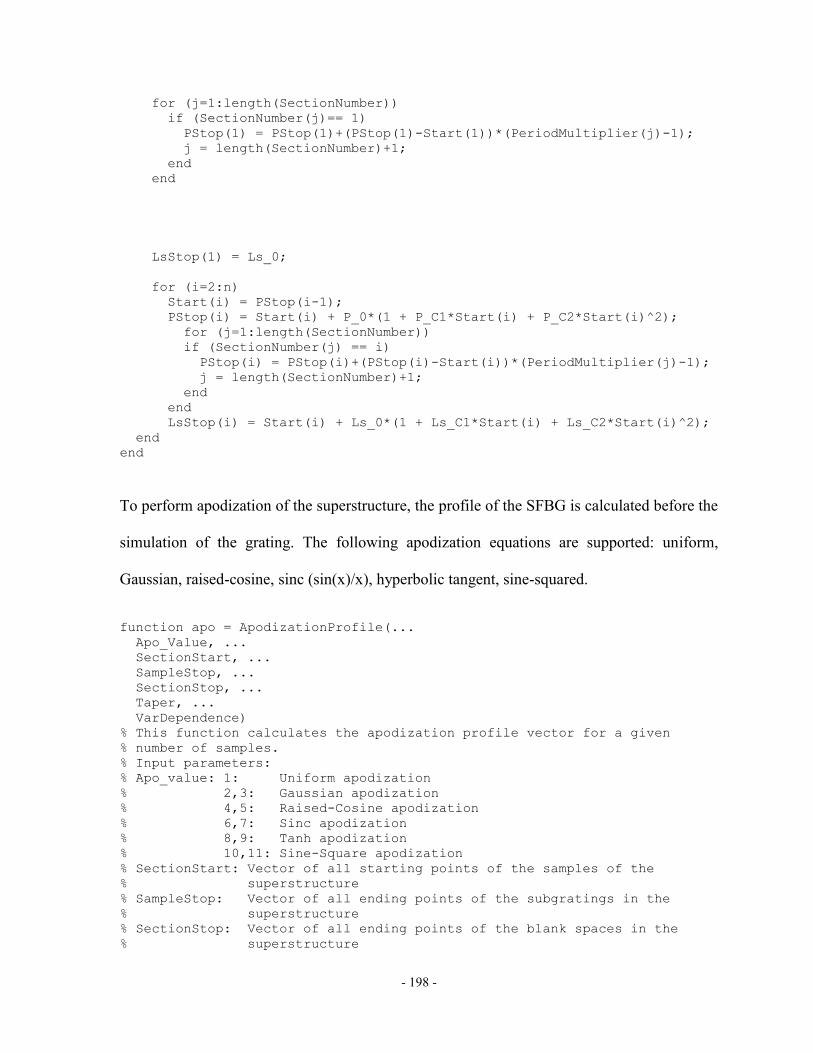
- 198 -

for (j=1:length(SectionNumber)) if (SectionNumber(j)== 1) PStop(1) = PStop(1)+(PStop(1)-Start(1))*(PeriodMultiplier(j)-1); j = length(SectionNumber)+1; end end

LsStop(1) = Ls_0;

for (i=2:n) Start(i) = PStop(i-1); PStop(i) = Start(i) + P_0*(1 + P_C1*Start(i) + P_C2*Start(i)^2); for (j=1:length(SectionNumber)) if (SectionNumber(j) == i) PStop(i) = PStop(i)+(PStop(i)-Start(i))*(PeriodMultiplier(j)-1); j = length(SectionNumber)+1; end end LsStop(i) = Start(i) + Ls_0*(1 + Ls_C1*Start(i) + Ls_C2*Start(i)^2); end end

To perform apodization of the superstructure, the profile of the SFBG is calculated before the

simulation of the grating. The following apodization equations are supported: uniform,

Gaussian, raised-cosine, sinc (sin(x)/x), hyperbolic tangent, sine-squared.

function apo = ApodizationProfile(... Apo_Value, ... SectionStart, ... SampleStop, ... SectionStop, ... Taper, ... VarDependence) % This function calculates the apodization profile vector for a given % number of samples. % Input parameters: % Apo_value: 1: Uniform apodization % 2,3: Gaussian apodization % 4,5: Raised-Cosine apodization % 6,7: Sinc apodization % 8,9: Tanh apodization % 10,11: Sine-Square apodization % SectionStart: Vector of all starting points of the samples of the % superstructure % SampleStop: Vector of all ending points of the subgratings in the % superstructure % SectionStop: Vector of all ending points of the blank spaces in the % superstructure

- 199 -

% Taper: Taper value required for Apo_value = 2, 3, 4 and 5. % This will shape the apodization profile. % VarDependence: 0: Apodization profile calculated as a function of the % position along the z-axis (along the length of the % fiber) % 1: Apodization profile calculated as a function of the % sample number

%

NbSamp = length(SectionStart); n = 0.5:1:NbSamp-0.5; SFBGLength = SectionStop(length(SectionStop)); z = SectionStart + (SampleStop-SectionStart)/2; % Find the middle of each

% sample

if (Apo_Value==1) %Uniform apo = ones(1, NbSamp); else if (Apo_Value==2||Apo_Value==3) %Gaussian if (VarDependence == 1) %n dependence apo = exp((-4*log(2).*(n-NbSamp/2).^2)./((NbSamp*Taper)^2)); else %z dependence apo = exp((-4*log(2).*(z-SFBGLength/2).^2)./((SFBGLength*Taper)^2)); end else if (Apo_Value==4||Apo_Value==5) %Raised-Cosine if (VarDependence == 1) %n dependence apo = 0.5*(1+cos(pi*(n-NbSamp/2)./(Taper*NbSamp))); else %z dependence apo = 0.5*(1+cos(pi*(z-SFBGLength/2)./(Taper*SFBGLength))); end else if (Apo_Value==6||Apo_Value==7) %Sinc if (VarDependence == 1) %n dependence apo = sinc((n-NbSamp/2)./(Taper*NbSamp)); else %z dependence apo = sinc((z-SFBGLength/2)./(Taper*SFBGLength)); end else if (Apo_Value==8||Apo_Value==9) %Tanh if (VarDependence == 1) %n dependence apo = tanh(Taper.*n./NbSamp).*tanh(Taper.*(1-n./NbSamp))+…

1-tanh(Taper/2).^2; else %z dependence apo = tanh(Taper.*z./SFBGLength).*tanh(Taper.*(1-…

z./SFBGLength))+1-tanh(Taper/2).^2; end else if (Apo_Value==10||Apo_Value==11) %Sine-Square if (VarDependence == 1) apo = sin(n/NbSamp*pi).^2; else apo = sin(z/SFBGLength*pi).^2; end

- 200 -

end end end end end end

Similarly, a subgrating may be apodized and a function has been created to perform the

calculation of this apodization profile.

function output = ApodizationProfileSample(... Apo_Value, ... NbPeriods, ... Taper) % This function calculates the apodization profile vector for a given % number of grating samples. % Input parameters: % Apo_value: 1: Uniform apodization % 2: Gaussian apodization % 3: Raised-Cosine apodization % 4: Sinc apodization % 5: Tanh apodization % 6: Sine-Square apodization % NbPeriods : Number of subdivisions inside the grating to simulate. % Taper: Taper value required for Apo_value = 2, 3, 4 and 5. % This will shape the apodization profile.

if (Apo_Value==1) %Uniform output = ones(1, NbPeriods); else if (Apo_Value==2) %Gaussian z = 0.5:1:NbPeriods-0.5; output = exp((-4*log(2).*(z-NbPeriods/2).^2)./((NbPeriods*Taper)^2)); clear z; else if (Apo_Value==3) %Raised-Cosine z = 0.5:1:NbPeriods-0.5; output = 0.5*(1+cos(pi*(z-NbPeriods/2)./(Taper*NbPeriods))); clear z else if (Apo_Value==4) %Sinc z = 0.5:1:NbPeriods-0.5; output = sinc((z-NbPeriods/2)./(Taper*NbPeriods)); clear z else if (Apo_Value==5) %Tanh z = 0.5:1:NbPeriods-0.5; output = tanh(Taper.*z./NbPeriods).*tanh(Taper.*(1-z./... NbPeriods))+1-tanh(Taper/2).^2; clear z

- 201 -

else if (Apo_Value==6) %Sine-Square z = 0.5:1:NbPeriods-0.5; output = sin(z/NbPeriods*pi).^2; clear z end end end end end end

In order to simulate an SFBG fabricated with a chirped phase mask, a function has been

created to return the Bragg wavelength given phase mask parameters and current position

along the z-axis. When using the TMM method to simulate gratings, samples are considered

to be small and the Bragg wavelength is approximated as constant for the entire length of the

sample.

function output = phasemask(... z, ... Length, ... Lambda_d, ... Chirp) % This function calculates the Bragg wavelength as position z based on % physical information of the phase mask (length, initial Bragg % wavelength, chirp). % Input parameters: % z: Current position along the length of the phase mask % Length: Physical length of the phase mask if z > Length, an error % is generated % Lambda_d: Initial Bragg wavelength (at z = 0) % Chirp: Chirp of the phasemask (may be 0)

if (x>Length) error('x larger than length of phase mask'); else output = x/Length*Chirp + Lambda_d; end

When processing the phase information of an SFBG, it is often necessary to unwrap the

phase curve. This is achieved with the following function:

function output = SBUnwrap(input, value, percentage) % This functions unwraps a phase curve. % Mandatory inputs:

- 202 -

% input: Phase curve to process % % Optional inputs: % value: Value equal to a phase jump. Defaults to pi. % Percentage: A jump may not be 100% of the value. Specify a reasonable % percentage of the value to consider as a phase jump given % the resolution of the phase curve.

if (nargin==3) else percentage = 0.99; end input2 = input(2:length(input)); input3 = input(1:length(input)-1); diff = input2-input3;

if (nargin==2) diff = -round(diff./(percentage*value)); else diff = -round(diff./(percentage*pi)); end diff = cumsum(diff); output(1) = input(1); if (nargin==2) output(2:length(input)) = input (2:length(input))+diff.*value; else output(2:length(input)) = input(2:length(input))+diff.*pi; end

With this information, it is now possible to simulate an SFBG using the TMM. The SFBG( )

function performs this calculation and allows to define and apodization profile for a

subgrating. This may be more representative of the actual SFBG fabricated as a subgrating is

often fabricated by a single exposure of the laser beam onto the fiber. The intensity profile of

the laser beam essentially apodizes the subgrating instead of creating a uniform refractive

index modulation as is often simulated in literature. The subgrating profile changes the

envelope that modulates the amplitude spectrum. The group delay response, on the other

hand, keeps approximately the same value in the pass band of the SFBG and this, for each

value of Ls. Fig. 85 (a) shows an SFBG simulated with a uniform subgrating profile and Fig.

- 203 -

85 (b) shows the refractive index profile, while Fig. 86 (a) shows an SFBG simulated with a

Gaussian subgrating profile, with a taper of 0.5 and Fig. 86 (b) shows its refractive index

profile.

(a)

(b)

Fig. 85. (a) Amplitude and (b) refractive index profile of an SFBG simulated with uniform

subgrating apodization. P0 = 0.6 mm, Ls = 0.3 mm, N = 40.

1540 1545 1550 1555 15600

0.2

0.4

0.6

0.8

1

(nm)

Re

fle

ctivity

0 5 10 15 20

1.447

1.4472

1.4474

x (mm)

- 204 -

(a)

(b)

Fig. 86. (a) Amplitude and (b) refractive index profile of an SFBG simulated with Gaussian

subgrating apodization, with a taper of 0.5. P0 = 0.6 mm, Ls = 0.3 mm, N = 40.

The SFBG( ) function source code is given below.

1540 1545 1550 1555 15600

0.2

0.4

0.6

0.8

1

(nm)

Re

fle

ctivity

0 5 10 15 20

1.447

1.4472

1.4474

x (mm)

- 205 -

function [Lambda Rx Disp Delay] = SFBG (... LambdaStart, ... LambdaStop, ... n_eff, ... del_n_eff, ... NumberPeriods, ... Apo_Value, ... Taper, ... VarDependence, ... NbSampleTMM, ... ApoS_Value, ... TaperSample, ... InitialPMPeriod, ... PMChirp, ... PMLength, ... SectionStart, ... SampleStop, ... SectionStop) % This function simulates an SFBG and returns a wavelength vector, % reflectivity vector, dispersion vector and group delay vector. % Input parameters: % LambdaStart: Start of the wavelength range to simulate % LambdaStop: End of the wavelength range to simulate % n_eff: Effective refractive index of the fiber % del_n_eff: Amplitude of the refractive index modulation % NumberPeriods: Number of samples in the superstructure % Apo_Value: Type of apodization profile. Refer to the help % from ApodizationProfileSample for more % information. % Taper: Taper value for some types of apodization profiles % VarDependence: 0: Apodization profile calculated as a function of % the position along the z-axis (along the length % of the fiber) % 1: Apodization profile calculated as a function of % the sample number % NbSampleTMM: Number of samples in a subgrating (for TMM % calculation) % ApoS_Value: Apodization profile of the subgrating % TaperSample: Taper value for the apodization profile of the % subgrating % InitialPMPeriod: Initial phase mask period % PMChirp: Phase mask chirp coefficient % PMLength: Physical length of the phase mask % SectionStart: Vector of all starting points of the samples of % the superstructure % SampleStop: Vector of all ending points of the subgratings in % the superstructure % SectionStop: Vector of all ending points of the blank spaces in % the superstructure

%

- 206 -

%%%%%%%%%%%%%%%%%%%%%%%%%%%%%%%%%%%%%%%%%%%%%%%%%%%%%%%%%%%%%%%%%%%%%%%%%%

% %%% Calculate Grating Length %%% %%%%%%%%%%%%%%%%%%%%%%%%%%%%%%%%%%%%%%%%%%%%%%%%%%%%%%%%%%%%%%%%%%%%%%%%%%

% [SectionStart SampleStop SectionStop] = SamplePeriodPosition( ... NumberPeriods, InitialPeriod, InitialLs, P_C1, P_C2, P_C3, P_C4, ... Ls_C1, Ls_C2, VarDependence, SectionNber, PeriodMult);

%%% Calculating Exposed Section Lengths %%% SectionLengths = SectionStop-SectionStart; SampleLengths = SampleStop-SectionStart;

%%%%%%%%%%%%%%%%%%%%%%%%%%%%%%%%%%%%%%%%%%%%%%%% %%% Preparing Display Percent Window %%% %%%%%%%%%%%%%%%%%%%%%%%%%%%%%%%%%%%%%%%%%%%%%%%%

NoMatrices = (NbSampleTMM+1)*NumberPeriods; Backscan = 0; if (Apo_Value==3||Apo_Value==5||Apo_Value==7||Apo_Value==9||Apo_Value==11) Backscan = 1; end % Equals to the number of TMM in the subgrating + the blank space and

% that, for all subgratings.

%%%%%%%%%%%%%%%%%%%%%%%%%%%%%%%%%%%%%%%%%%%%%%%% %%% Grating profile %%% %%%%%%%%%%%%%%%%%%%%%%%%%%%%%%%%%%%%%%%%%%%%%%%% MaxPeriodAmplitudes = ApodizationProfile(Apo_Value, SectionStart, ... SampleStop, SectionStop, Taper, VarDependence);

%%%%%%%%%%%%%%%%%%%%%%%%%%%%%%%%%%%%%%%%%%%%%%%% %%% Initialization %%% %%%%%%%%%%%%%%%%%%%%%%%%%%%%%%%%%%%%%%%%%%%%%%%% % At leat 1000 samples for each nm of spectrum required to avoid jumps in % time delay. NoSamples = round((LambdaStop-LambdaStart)*1e9*1000); Lambda = LambdaStart:(LambdaStop-LambdaStart)/(NoSamples-1):LambdaStop; z_pos = 0; SubSectionLength = SampleLengths./NbSampleTMM;

%%%%%%%%%%%%%%%%%%%%%%%%%%%%%%%%%%%%%%%%%%%%%%%% %%% RUN SIMULATION %%%%%%%%%%%%%%%%%%%%%%%%%%%%%%%%%%%%%%%%%%%%%%%% for i = 1:NumberPeriods,

%Subgrating PeriodAmplitudes = ApodizationProfileSample(ApoS_Value, ... NbSampleTMM, TaperSample); PeriodAmplitudes = PeriodAmplitudes * MaxPeriodAmplitudes(i); for j = 1:NbSampleTMM, Lambda_d = phasemask(z_pos+SubSectionLength(i)/2, PMLength, ... InitialPMPeriod, PMChirp); if (Backscan==1) [TT11, TT12, TT21, TT22] = TransferMatrixBS(Lambda, ...

- 207 -

Lambda_d, n_eff, del_n_eff, 1, SubSectionLength(i), ... PeriodAmplitudes(j)); else [TT11, TT12, TT21, TT22] = TransferMatrix(Lambda, ...

Lambda_d, ... n_eff, del_n_eff, 1, SubSectionLength(i), ... PeriodAmplitudes(j)); end z_pos = z_pos + SubSectionLength(i); if (j==1&&i==1) T11 = TT11; T12 = TT12; T21 = TT21; T22 = TT22; else TTT11 = T11.*TT11 + T12.*TT21; TTT12 = T11.*TT12 + T12.*TT22; TTT21 = T21.*TT11 + T22.*TT21; TTT22 = T21.*TT12 + T22.*TT22; T11 = TTT11; T12 = TTT12; T21 = TTT21; T22 = TTT22; end end

% Blank Space z_pos = SampleStop(i); Lambda_d = phasemask(z_pos+(SectionStop(i)-SampleStop(i))/2, ... PMLength, InitialPMPeriod, PMChirp); if (Backscan==1) [TT11, TT12, TT21, TT22] = TransferMatrixBS(Lambda, Lambda_d, ... n_eff, del_n_eff, 0, SectionStop(i)-SampleStop(i), 1); else [TT11, TT12, TT21, TT22] = TransferMatrix(Lambda, Lambda_d, ... n_eff, del_n_eff, 0, SectionStop(i)-SampleStop(i), 1); end z_pos = SectionStop(i);

TTT11 = T11.*TT11 + T12.*TT21; TTT12 = T11.*TT12 + T12.*TT22; TTT21 = T21.*TT11 + T22.*TT21; TTT22 = T21.*TT12 + T22.*TT22; T11 = TTT11; T12 = TTT12; T21 = TTT21; T22 = TTT22;

end

rho = T12./T11; Rx = abs(rho).^2;

- 208 -

step = (3e8/Lambda(length(Lambda)) - 3e8/Lambda(1))/length(Lambda);

phase = angle(rho); phase = SBUnwrap(phase); phase1 = phase(1:length(phase)-1); phase2 = phase(2:length(phase)); Lambda1 = Lambda(1:length(Lambda)-1); Lambda2 = Lambda(2:length(Lambda)); step = Lambda1-Lambda2; Delay = (phase2-phase1).*Lambda(2:length(Lambda)).^2./(2*pi.*step*3e8); Disp1 = Delay(1:length(Delay)-1); Disp2 = Delay(2:length(Delay)); Disp = (Disp2-Disp1)./(Lambda(2)-Lambda(1)); Disp(length(Disp)+1)=Disp(length(Disp));

In order to run the linearization algorithm continuously without user intervention, several

processing functions are required. From an SFBG simulation, the amplitude and phase

response of the SFBG as a function of wavelength are stored in a file. At each iteration of the

linearization algorithm,

From these vectors, the +/- 1st spectral orders have to be identified and their 3-dB bandwidths

are needed to calculate the normalized group delay error with respect to the target dispersion.

The first task, identifying the +/-1st spectral orders is performed by the function

Find2ndPeak( ).

- 209 -

function value = Find2ndPeak(... Vector, ... Index, ... Threshold, ... Step) % This function parses a vector to search for the location of a second % peak from a reference initial peak. % Input parameters: % Vector: Vector to analyse, in which to find the second peak % Index: Index of the first peak % Theshold: Value of the vector where a peak starts/stops % Step: Safety margin to avoid detecting sidelobes as peaks. The % value provided must be in indices % % % Step % |<->| |<------->| % /\ | | /\ % || | | || % || | | || % treshold -- /\/ \/\ | /\/ \/\ % /\/ \/\ /\/ \/\ % ..... ........ % 1. Start at first peak % 2. Find point where threshold is passed (falling) % 3. Skip a length equal to the step % 4. Find point where threshold is passed (rising) % 5. Scan until threshold is passed (falling) % 6. Scan for a length of step. If threshold is passed again (rising), % continue scanning until threshold is passed again (falling). Repeat % step 6.

value = 0; State = 0;

% The increment is set to 50 to run faster and give enough precision. for i = Index:50:length(Vector), if State == 0, if (Vector(i)<=Threshold), State = 1; i = GetIndex(Vector, Vector(i)+Step); end else if State == 1, if (Vector(i)>=Threshold), State = 2; Max_Value = Vector(i); value = i; end else if State == 2, if (Vector(i)>=Max_Value), Max_Value = Vector(i); value = i; end if (Vector(i)<=Threshold), State = 3; StepIndex = 0; end

- 210 -

else if (State == 3) StepIndex = StepIndex+1; if (StepIndex <= Step) if (Vector(i)>=Threshold), State = 2; end else i = length(Vector)+10; end end end end end end

if (value == 0), err('Error: value = 0'); end

The following function BW_3dB( ) extracts the 3-dB bandwidth of the +/-1st orders

previously found.

function [Index0, Index1] = BW_3dB(... amplitude, ... CenterIndex, ... Bandwidth) % This function takes a normalized function (with its maximum at 0 dB) and % the index of a start point somewhere inside the pass-band of the order % of interest. The function then searches for the X-dB points on each side % of the start point, where X is defined as an input parameter. % Input parameters % amplitude: Amplitude input vector % CenterIndex: Index of a start point somewhere inside the pass-band % of the order of interest % Bandwidth: Amplitude value considered as the threshold of % interest

- 211 -

StartIndex = 0; EndIndex = 0; MaxValue = amplitude(CenterIndex);

for i=CenterIndex:-1:1, if (amplitude(i)>MaxValue) MaxValue = amplitude(i); end

if (amplitude(i)>=MaxValue-Bandwidth) StartIndex = i; else break; end end

for i=CenterIndex:length(amplitude), if (amplitude(i)>MaxValue) MaxValue = amplitude(i); end

if (amplitude(i)>=MaxValue-Bandwidth) EndIndex = i; else break; end end

% Redo the lower wavelength side as the max value may be higher now. for i=CenterIndex:-1:1, if (amplitude(i)>=MaxValue-Bandwidth) StartIndex = i; else break; end end

if (StartIndex == 0) err('Error: StartIndex = 0'); end if (EndIndex == 0) err('Error: EndIndex = 0'); end

Index0 = StartIndex; Index1 = EndIndex;

- 212 -

Finally, a function, NonLinearAnalysis( ), calculating the error of the group delay response

within the 3-dB bandwidth of the +/-1st orders of the SFBG with respect to a target dispersion

value is called. The function finds a linear curve with a slope equal to the target dispersion

and calculates the error value between the group delay curve and this reference linear curve.

The error is then normalized with respect to the 3-dB bandwidth.

function Error = NonLinearAnalysis(... x, ... y, ... target_disp, ... Str1, ... Str2, ... Str3, ... Str4, ... FileName, ... Do_Plot) % This function calculates the group delay error with respect to a target % dispersion value. First, the group delay response is submitted to a % linear regression to find its center point through which the linear % curve of the reference target dispersion will pass. From this, a linear % curve is defined as a function of the x variable and error between the % group delay curve and this reference linear curve is calculated and % normalized with respect to the bandwidth of interest.

[a, b] = RegLin(x, y, [1, length(x)]); y_mid = a*x(round(length(x)/2))+b;

if (Do_Plot) figure; plot(x*1e9,y*1e12, 'r'); hold on; plot(x*1e9, (a*x+b)*1e12, 'b'); end

new_b = y_mid - target_disp*x(round(length(x)/2));

a = target_disp; b = new_b;

if (Do_Plot) plot(x*1e9, (a*x+b)*1e12, ':k');

end

Error = 0; for i=1:length(x), Error = Error + ((y(i)*1e12 - (a*x(i)+b)*1e12)^2)*(x(2)-x(1)); end

- 213 -

Error = Error / (x(length(x))-x(1));

dlmwrite(FileName, Str1, '-append', 'delimiter', '', 'newline', 'pc'); dlmwrite(FileName, Str2, '-append', 'delimiter', '', 'newline', 'pc'); dlmwrite(FileName, Str3, '-append', 'delimiter', '', 'newline', 'pc'); dlmwrite(FileName, Str4, '-append', 'delimiter', '', 'newline', 'pc'); dlmwrite(FileName, num2str(Error), '-append', 'delimiter', '', 'newline',

'pc'); dlmwrite(FileName, ' ', '-append', 'delimiter', '', 'newline', 'pc');

To calculate the error with respect to a target dispersion value, the NonLinearAnalysis( )

function makes use of a linear regression function, RegLin.

function [a, b] = RegLin(x, y, index)

% index = [StartIndex, StopIndex], inclusive (e.g. [1, 25] will consider % the point 1 to 25, inclusively.

n = index(2) - index(1) + 1;

Sy = 0; Sx = 0; Sx2 = 0; Sxy = 0;

for i=index(1):index(2), Sy = Sy + y(i); Sx = Sx + x(i); Sx2 = Sx2 + x(i)^2; Sxy = Sxy + x(i)*y(i); end

a = (Sxy - (Sx*Sy)/n)/(Sx2-(Sx^2)/n); b = (Sy - a*Sx)/n;

Once the simulation displays the optimal chirp coefficient values for a target SFBG and a

target dispersion value, a graphical user interface (GUI) can be used to simulate this grating

and view its amplitude and group delay responses. Fig. 87 shows the GUI created in Matlab

- 214 -

to simulate SFBGs. The novelty of this tool is that it allows the simulation of SFBG with

equivalent chirp and equivalent phase shift based on the linearization method presented.

Fig. 87. Graphical user interface tool to simulate SFBG with equivalent chirp and/or with

equivalent phase shift based on Matlab code.

On the right hand side, the section entitled “Simulation Parameters” take the user’s input for

the SFBG simulation. Wavelength ranges, refractive index of the fiber and refractive index

modulation can be specified. The superstructure attributes can then be defined and the grating

length is updated live. This ensures that the user doesn’t simulate a grating that cannot be

fabricated, should the length of the grating exceed the physical length of the phase masks

available. The apodization profile can be specified for the superstructure as well as for the

subgrating. The tool supports the simulation of equivalent chirp and equivalent phase shifts.

Finally, the parameters of the phase mask to be used for the simulation can be entered.

- 215 -

Chirped phase masks are supported and an entry field has been added for the phase mask

chirp value.

The section “Results” is located on the left hand side. The first graph shows the amplitude

response of the simulated SFBG and a linear/log option is present. The second graph shows

the phase response of the SFBG and offers the option to view the group delay or the

dispersion response. Finally, the third graph shows a representation of the refractive index

profile of the SFBG.

For all graphs of the “Result” section, controls are available to view the graphs in a standard

Matlab window, as shown in Fig. 88, and, in the case of the amplitude and phase spectra, to

save the figures for later processing and viewing.

Fig. 88. Viewing figures in standard Matlab windows using the graphical user interface tool.

- 216 -

The source code for the GUI tool is found below:

File: Main.m

clc; clear;

%%% DRAW EVERYTHING %%%

ScrSize = get(0, 'ScreenSize');

%%% Draw window %%% WinMarginX = 0.1; WinMarginY = 0.1; window = figure; set(window, 'Color', [236/255 233/255 216/255]); bgcolor = get(window, 'Color'); set(window, 'units', 'normalized'); set(window, 'position', [WinMarginX, WinMarginY, 1-2*WinMarginX, .. 1-2*WinMarginY]); set(window, 'Name', ... 'Superstructure Fiber Bragg Gratings (c) 2007-2013 Sebastien Blais', ... 'NumberTitle', 'off', 'MenuBar', 'figure', 'Resize', 'off', ... 'toolbar', 'figure');

TitleWidth = 1; TitleHeight = 0.025; FigMarginX = 0.025; FigMarginY = 0.025; ButtonWidth = 0.055; ButtonHeight = 0.035; ControlWidth = 0.05625; ControlHeight = 0.035; ApoDropDownWidth = 0.145; ApoSampleDropDownWidth = 0.23; PhaseShiftWidth = 0.1875; UnitsWidth = 0.025; UnitsHeight = 0.028; AxesWidth = 0.5-3*FigMarginX-ButtonWidth; AxesHeight = 0.5-7*FigMarginX-ButtonWidth; Axe1VertCenter = 1-(3*FigMarginY+AxesHeight/2); Axe2VertCenter = 1-(4*FigMarginY+1.5*AxesHeight); Axe3_4VertCenter = 0.5-AxesHeight-0.5*FigMarginY;

FontSize = floor(ControlHeight*ScrSize(4)/4);

%%% Draw title %%% TITLE = uicontrol('style', 'text', 'FontSize', FontSize+1, ... 'FontUnits', 'points', 'FontWeight', 'bold', ... 'HorizontalAlignment', 'center', 'String', ... 'Simulation of Superstructure FBGs',... 'BackgroundColor', bgcolor, 'units', 'normalized', 'position', ... [(1-TitleWidth)/2 1-TitleHeight TitleWidth TitleHeight]);

- 217 -

%%% Draw Result Panel %%% ResultPanel = uipanel('title', 'Results', 'FontSize', FontSize, ... 'FontUnits', 'points',... 'BackgroundColor', bgcolor, 'units', 'normalized', ... 'Position', [FigMarginX FigMarginY 0.5-FigMarginX 1-2*FigMarginY]);

Scale = [0 0 0]; %0: Lin, 1: Log 0: Rx, 1: Tx 0: Delay, 1: Disp

%%% Draw graphs and associated buttons %%% ButtonRx = uicontrol('style', 'pushbutton', 'FontSize', FontSize, ... 'FontUnits', 'points',... 'BackgroundColor', bgcolor, 'string', 'Rx', 'units', 'normalized',... 'position', [2*FigMarginX+AxesWidth ... Axe1VertCenter+(2*ButtonHeight+1.25*FigMarginY) ButtonWidth ... ButtonHeight], 'enable', 'off',... 'callback', 'Scale = DisplayRx(window, graph1, Scale, Lambda, Rx);'); ButtonTx = uicontrol('style', 'pushbutton', 'FontSize', FontSize, ... 'FontUnits', 'points',... 'BackgroundColor', bgcolor, 'string', 'Tx', 'units', 'normalized',... 'position', [2*FigMarginX+AxesWidth Axe1VertCenter+... (1*ButtonHeight+0.75*FigMarginY) ButtonWidth ButtonHeight], ... 'enable', 'off',... 'callback', 'Scale = DisplayTx(window, graph1, Scale, Lambda, Rx);'); ButtonLin = uicontrol('style', 'pushbutton', 'FontSize', FontSize, ... 'FontUnits', 'points',... 'BackgroundColor', bgcolor, 'string', 'Lin', 'units', 'normalized',... 'position', [2*FigMarginX+AxesWidth Axe1VertCenter+... (0.25*FigMarginY) ButtonWidth ButtonHeight], 'enable', 'off',... 'callback', 'Scale = DisplayLin(window, graph1, Scale, Lambda, Rx);'); ButtonLog = uicontrol('style', 'pushbutton', 'FontSize', FontSize, ... 'FontUnits', 'points',... 'BackgroundColor', bgcolor, 'string', 'Log', 'units', 'normalized',... 'position', [2*FigMarginX+AxesWidth Axe1VertCenter-... (ButtonHeight+0.25*FigMarginY) ButtonWidth ButtonHeight], ... 'enable', 'off',... 'callback', 'Scale = DisplayLog(window, graph1, Scale, Lambda, Rx);'); ButtonEnlarge1 = uicontrol('style', 'pushbutton', 'FontSize', ... FontSize, 'FontUnits', 'points',... 'BackgroundColor', bgcolor, 'string', 'View', 'units',

'normalized',... 'position', [2*FigMarginX+AxesWidth Axe1VertCenter-... (2*ButtonHeight+0.75*FigMarginY) ButtonWidth ButtonHeight], ... 'enable', 'off',... 'callback', 'Enlarge1(Lambda, Rx, Scale)'); ButtonSave1 = uicontrol('style', 'pushbutton', 'FontSize', FontSize, ... 'FontUnits', 'points',... 'BackgroundColor', bgcolor, 'string', 'Save', 'units',

'normalized',... 'position', [2*FigMarginX+AxesWidth Axe1VertCenter-... (3*ButtonHeight+1.25*FigMarginY) ButtonWidth ButtonHeight], ... 'enable', 'off',... 'callback', 'Save(1)'); ButtonDelay = uicontrol('style', 'pushbutton', 'FontSize', FontSize, ... 'FontUnits', 'points',...

- 218 -

'BackgroundColor', bgcolor, 'string', 'Delay', 'units', ... 'normalized', ... 'position', [2*FigMarginX+AxesWidth Axe2VertCenter+... (ButtonHeight+0.75*FigMarginY) ButtonWidth ButtonHeight], ... 'enable', 'off',... 'callback', ... 'Scale = DisplayDelay(window, graph2, Scale, Lambda, Delay);'); ButtonDisp = uicontrol('style', 'pushbutton', 'FontSize', FontSize, ... 'FontUnits', 'points',... 'BackgroundColor', bgcolor, 'string', 'Disp', 'units', ... 'normalized', ... 'position', [2*FigMarginX+AxesWidth Axe2VertCenter+ ... (0.25*FigMarginY) ButtonWidth ButtonHeight], 'enable', 'off',... 'callback', ... 'Scale = DisplayDisp(window, graph2, Scale, Lambda, Disp);'); ButtonEnlarge2 = uicontrol('style', 'pushbutton', 'FontSize', ... FontSize, 'FontUnits', 'points',... 'BackgroundColor', bgcolor, 'string', 'View', 'units', ... 'normalized',... 'position', [2*FigMarginX+AxesWidth Axe2VertCenter-... (ButtonHeight+0.25*FigMarginY) ButtonWidth ButtonHeight], ... 'enable', 'off',... 'callback', 'Enlarge2(Lambda, Disp, Delay, Scale)'); ButtonSave2 = uicontrol('style', 'pushbutton', 'FontSize', FontSize, ... 'FontUnits', 'points',... 'BackgroundColor', bgcolor, 'string', 'Save', 'units', ... 'normalized',... 'position', [2*FigMarginX+AxesWidth Axe2VertCenter-... (2*ButtonHeight+0.75*FigMarginY) ButtonWidth ButtonHeight], ... 'enable', 'off',... 'callback', 'Save(2)'); Button_A_and_P = uicontrol('style', 'pushbutton', 'FontSize', ... FontSize, 'FontUnits', 'points',... 'BackgroundColor', bgcolor, 'string', 'A & P', 'units', ... 'normalized',... 'position', [2*FigMarginX+AxesWidth Axe2VertCenter-... (4*ButtonHeight+1.75*FigMarginY) ButtonWidth ButtonHeight],... 'callback', 'Enlarge4(Lambda, Rx, Disp, Delay, Scale)'); ButtonEnlarge3 = uicontrol('style', 'pushbutton', 'FontSize', ... FontSize, 'FontUnits', 'points',... 'BackgroundColor', bgcolor, 'string', 'View', 'units', ... 'normalized',... 'position', [2*FigMarginX+AxesWidth Axe3_4VertCenter-... (0.5*ButtonHeight) ButtonWidth ButtonHeight],... 'callback', ... 'Enlarge3(n_eff, del_n_eff, InitialPeriod, InitialLs, NumberPeriods,

Apodization, Taper, VarDependence, NbSampleTMM, ApoSample, TaperSample,

SectionNber, PeriodMult, PeriodChirpC1, PeriodChirpC2, LsChirpC1,

LsChirpC2, InitialPMPeriod, PMChirp, PMLength)'); Button_n_eff = uicontrol('style', 'pushbutton', 'FontSize', FontSize, ... 'FontUnits', 'points',... 'BackgroundColor', bgcolor, 'string', 'n_eff', 'units', ... 'normalized',... 'position', [2*FigMarginX+AxesWidth Axe3_4VertCenter-... (1.5*ButtonHeight+0.5*FigMarginY) ButtonWidth ButtonHeight],... 'callback', ...

- 219 -

'Enlarge5(n_eff, del_n_eff, InitialPeriod, InitialLs, NumberPeriods,

Apodization, Taper, VarDependence, NbSampleTMM, ApoSample, TaperSample,

SectionNber, PeriodMult, PeriodChirpC1, PeriodChirpC2, LsChirpC1,

LsChirpC2, InitialPMPeriod, PMChirp, PMLength)');

graph1 = axes; set(graph1, 'FontSize', FontSize,... 'OuterPosition', [2*FigMarginX 1-3*FigMarginY-AxesHeight AxesWidth ... AxesHeight]); title('Amplitude Response'); xlabel('\lambda (nm)'); ylabel('Amplitude Response');

graph2 = axes; set(graph2, 'FontSize', FontSize,... 'OuterPosition', [2*FigMarginX 1-4*FigMarginY-2*AxesHeight ... AxesWidth AxesHeight]); xlabel('\lambda (nm)'); ylabel('Phase Response'); title('Phase Response');

graph3 = axes; set(graph3, 'FontSize', FontSize,... 'OuterPosition', [2*FigMarginX 3*FigMarginY+1/3*(1-2*AxesHeight-... 8*FigMarginY) AxesWidth 2/3*(1-2*AxesHeight-8*FigMarginY)]); xlabel('x (mm)'); title('Refractive Index Profile');

graph4 = axes; set(graph4, 'FontSize', FontSize,... 'OuterPosition', [2*FigMarginX 2*FigMarginY AxesWidth 1/3*... (1-2*AxesHeight-8*FigMarginY)]); xlabel('\lambda (nm)');

%%% Draw Parameter Panel %%% ParametersPanel = uipanel('title', 'Simulation Parameters', ... 'FontSize', FontSize, 'FontUnits', 'points',... 'BackgroundColor', bgcolor, 'units', 'normalized',... 'Position', [0.5+FigMarginX FigMarginY 0.5-2*FigMarginX ... 1-2*FigMarginY]);

%%% Draw simulation parameters %%% LambdaStart = uicontrol('style', 'edit', 'FontSize', FontSize,... 'FontUnits', 'points', 'units', 'normalized',... 'position', [0.5+2*FigMarginX 1-3*FigMarginY-ControlHeight ... ControlWidth ControlHeight],... 'string', '1545', 'backgroundcolor', 'white', 'Callback',...

- 220 -

'UpdateGUI(window, LambdaStart, LambdaStop, n_eff, del_n_eff,

InitialPeriod, InitialLs, NumberPeriods, GratingLength, Apodization,

Taper, VarDependence, NbSampleTMM, ApoSample, TaperSample, SectionNber,

PeriodMult, PeriodChirpC1, PeriodChirpC2, LsChirpC1, LsChirpC2,

InitialPMPeriod, PMChirp, PMLength, Message, graph3, graph4)'); LambdaStartTxt = axes; set(LambdaStartTxt, 'units', 'normalized', 'Color', 'none', ... 'visible', 'off', 'FontSize', FontSize,... 'position', [0.5+2*FigMarginX 1-3*FigMarginY-2*ControlHeight ... ControlWidth ControlHeight]); text(0.5,0.5,'\lambda_s_t_a_r_t', 'BackgroundColor', bgcolor, ... 'HorizontalAlignment', 'center',... 'VerticalAlignment', 'middle', 'FontSize', FontSize); uicontrol('style', 'text', 'FontSize', FontSize, 'FontUnits', 'points',... 'BackgroundColor', bgcolor, 'string', 'nm', 'units', ... 'normalized',... 'position', [0.5+2*FigMarginX+ControlWidth ... 1-3*FigMarginY-ControlHeight UnitsWidth UnitsHeight]);

LambdaStop = uicontrol('style', 'edit', 'FontSize', FontSize, ... 'FontUnits', 'points', 'units', 'normalized',... 'position', [0.5+3*FigMarginX+ControlWidth+UnitsWidth ... 1-3*FigMarginY-ControlHeight ControlWidth ControlHeight],... 'string', '1555', 'backgroundcolor', 'white', 'Callback',... 'UpdateGUI(window, LambdaStart, LambdaStop, n_eff, del_n_eff,




InitialPMPeriod, PMChirp, PMLength, Message, graph3, graph4)'); LambdaStopTxt = axes; set(LambdaStopTxt, 'units', 'normalized', 'Color', 'none', 'visible', ... 'off', 'FontSize', FontSize,... 'position', [0.5+3*FigMarginX+ControlWidth+UnitsWidth ... 1-3*FigMarginY-2*ControlHeight ControlWidth ControlHeight]); text(0.5,0.5,'\lambda_s_t_o_p', 'BackgroundColor', bgcolor, ... 'HorizontalAlignment', 'center',... 'VerticalAlignment', 'middle', 'FontSize', FontSize); uicontrol('style', 'text', 'FontSize', FontSize, 'FontUnits', ... 'points', 'BackgroundColor', bgcolor,... 'string', 'nm', 'units', 'normalized', ... 'position', [0.5+3*FigMarginX+2*ControlWidth+UnitsWidth ... 1-3*FigMarginY-ControlHeight UnitsWidth UnitsHeight]);

n_eff = uicontrol('style', 'edit', 'FontSize', FontSize, 'FontUnits', ... 'points', 'units', 'normalized',... 'position', [0.5+4*FigMarginX+2*ControlWidth+2*UnitsWidth ... 1-3*FigMarginY-ControlHeight ControlWidth ControlHeight],... 'string', '1.447', 'backgroundcolor', 'white', 'Callback',... 'UpdateGUI(window, LambdaStart, LambdaStop, n_eff, del_n_eff,




InitialPMPeriod, PMChirp, PMLength, Message, graph3, graph4)');

- 221 -

n_effTxt = axes; set(n_effTxt, 'units', 'normalized', 'Color', 'none', 'visible', ... 'off', 'FontSize', FontSize,... 'position', [0.5+4*FigMarginX+2*ControlWidth+2*UnitsWidth ... 1-3*FigMarginY-2*ControlHeight ControlWidth ControlHeight]); text(0.5,0.5,'n_e_f_f', 'BackgroundColor', bgcolor, ... 'HorizontalAlignment', 'center',... 'VerticalAlignment', 'middle', 'FontSize', FontSize);

del_n_eff = uicontrol('style', 'edit', 'FontSize', FontSize, ... 'FontUnits', 'points', 'units', 'normalized',... 'position', [0.5+5*FigMarginX+3*ControlWidth+3*UnitsWidth ... 1-3*FigMarginY-ControlHeight ControlWidth ControlHeight],... 'string', '0.0005', 'backgroundcolor', 'white', 'Callback',... 'UpdateGUI(window, LambdaStart, LambdaStop, n_eff, del_n_eff,




InitialPMPeriod, PMChirp, PMLength, Message, graph3, graph4)'); del_n_effTxt = axes; set(del_n_effTxt, 'Color', 'none', 'visible', 'off', 'units', ... 'normalized', 'FontSize', FontSize,... 'position', [0.5+5*FigMarginX+3*ControlWidth+3*UnitsWidth ... 1-3*FigMarginY-2*ControlHeight ControlWidth ControlHeight]); text(0.5,0.5,'\deltan_e_f_f', 'BackgroundColor', bgcolor, ... 'HorizontalAlignment', 'center',... 'VerticalAlignment', 'middle', 'FontSize', FontSize);

%%% Divider %%% uicontrol('style', 'text', 'FontSize', FontSize, 'FontUnits', ... 'points', 'FontWeight', 'bold', 'BackgroundColor', bgcolor,... 'string', 'Superstructure Parameters', 'units', 'normalized', ... 'HorizontalAlignment', 'left',... 'position', [0.5+2*FigMarginX 1-4*FigMarginY-3*ControlHeight ... 0.5-4*FigMarginX ControlHeight]);

%%% Draw Superstructure Parameters %%% InitialPeriod = uicontrol('style', 'edit', 'FontSize', FontSize,... 'FontUnits', 'points', 'units', 'normalized',... 'position', [0.5+2*FigMarginX 1-4*FigMarginY-4*ControlHeight ... ControlWidth ControlHeight],... 'string', '0.6', 'backgroundcolor', 'white', 'Callback',... 'UpdateGUI(window, LambdaStart, LambdaStop, n_eff, del_n_eff,




InitialPMPeriod, PMChirp, PMLength, Message, graph3, graph4)'); InitialPeriodTxt = axes; set(InitialPeriodTxt, 'units', 'normalized', 'Color', 'none', ... 'visible', 'off', 'FontSize', FontSize,...

- 222 -

'position', [0.5+2*FigMarginX 1-4*FigMarginY-5*ControlHeight ... ControlWidth ControlHeight]); text(0.5,0.5,'P_i_n_i_t_i_a_l', 'BackgroundColor', bgcolor, ... 'HorizontalAlignment', 'center',... 'VerticalAlignment', 'middle', 'FontSize', FontSize); uicontrol('style', 'text', 'FontSize', FontSize, 'FontUnits', 'points',... 'BackgroundColor', bgcolor, 'string', 'mm', 'units', 'normalized',... 'position', [0.5+2*FigMarginX+ControlWidth ... 1-4*FigMarginY-4*ControlHeight UnitsWidth UnitsHeight]);

InitialLs = uicontrol('style', 'edit', 'FontSize', FontSize,... 'FontUnits', 'points', 'units', 'normalized',... 'position', [0.5+3*FigMarginX+ControlWidth+UnitsWidth ... 1-4*FigMarginY-4*ControlHeight ControlWidth ControlHeight],... 'string', '0.3', 'backgroundcolor', 'white', 'Callback',... 'UpdateGUI(window, LambdaStart, LambdaStop, n_eff, del_n_eff,




InitialPMPeriod, PMChirp, PMLength, Message, graph3, graph4)'); InitialLsTxt = axes; set(InitialLsTxt, 'units', 'normalized', 'Color', 'none', 'visible', ... 'off', 'FontSize', FontSize,... 'position', [0.5+3*FigMarginX+ControlWidth+UnitsWidth ... 1-4*FigMarginY-5*ControlHeight ControlWidth ControlHeight]); text(0.5,0.5,'Ls_i_n_i_t_i_a_l', 'BackgroundColor', bgcolor, ... 'HorizontalAlignment', 'center',... 'VerticalAlignment', 'middle', 'FontSize', FontSize); uicontrol('style', 'text', 'FontSize', FontSize, 'FontUnits', 'points',... 'BackgroundColor', bgcolor, 'string', 'mm', 'units', 'normalized',... 'position', [0.5+3*FigMarginX+2*ControlWidth+UnitsWidth ... 1-4*FigMarginY-4*ControlHeight UnitsWidth UnitsHeight]);

NumberPeriods = uicontrol('style', 'edit', 'FontSize', FontSize, ... 'FontUnits', 'points', 'units', 'normalized',... 'position', [0.5+4*FigMarginX+2*ControlWidth+2*UnitsWidth ... 1-4*FigMarginY-4*ControlHeight ControlWidth ControlHeight],... 'string', '40', 'backgroundcolor', 'white', 'Callback',... 'UpdateGUI(window, LambdaStart, LambdaStop, n_eff, del_n_eff,




InitialPMPeriod, PMChirp, PMLength, Message, graph3, graph4)'); NumberPeriodsTxt = axes; set(NumberPeriodsTxt, 'units', 'normalized', 'Color', 'none', ... 'visible', 'off', 'FontSize', FontSize,... 'position', [0.5+4*FigMarginX+2*ControlWidth+2*UnitsWidth ... 1-4*FigMarginY-5*ControlHeight ControlWidth ControlHeight]); text(0.5,0.5,'# Periods', 'BackgroundColor', bgcolor, ... 'HorizontalAlignment', 'center',... 'VerticalAlignment', 'middle', 'FontSize', FontSize);

GratingLength = uicontrol('style', 'edit', 'FontSize', FontSize, ... 'FontUnits', 'points', 'units', 'normalized',... 'position', [0.5+5*FigMarginX+3*ControlWidth+3*UnitsWidth ... 1-4*FigMarginY-4*ControlHeight ControlWidth ControlHeight],...

- 223 -

'string', '24', 'backgroundcolor', 'white', 'Enable', 'off', ... 'Callback',... 'UpdateGUI(window, LambdaStart, LambdaStop, n_eff, del_n_eff,




InitialPMPeriod, PMChirp, PMLength, Message, graph3, graph4)'); GratingLengthTxt = axes; set(GratingLengthTxt, 'units', 'normalized', 'Color', 'none', ... 'visible', 'off', 'FontSize', FontSize,... 'position', [0.5+5*FigMarginX+3*ControlWidth+3*UnitsWidth ... 1-4*FigMarginY-5*ControlHeight ControlWidth ControlHeight]); text(0.5,0.5,'Grating Length', 'BackgroundColor', bgcolor, ... 'HorizontalAlignment', 'center',... 'VerticalAlignment', 'middle', 'FontSize', FontSize); uicontrol('style', 'text', 'FontSize', FontSize, 'FontUnits', ... 'points', 'BackgroundColor', bgcolor,... 'string', 'mm', 'units', 'normalized',... 'position', [0.5+5*FigMarginX+4*ControlWidth+3*UnitsWidth ... 1-4*FigMarginY-4*ControlHeight UnitsWidth UnitsHeight]);

Apodization = uicontrol('style', 'popupmenu', 'FontSize', FontSize, ... 'FontUnits', 'points', 'units', 'normalized',... 'position', [0.5+2*FigMarginX 1-5*FigMarginY-6*ControlHeight ... ApoDropDownWidth ControlHeight],... 'string', 'Uniform|Gaussian|Gaussian w. backscan|Raised-Cosine|Raised-

Cosine w. backscan|Sinc|Sinc w. backscan|Tanh|Tanh w. backscan|Sine-

Square|Sine-Square w. backscan', 'HorizontalAlignment', 'center',... 'Callback',... 'UpdateGUI(window, LambdaStart, LambdaStop, n_eff, del_n_eff,




InitialPMPeriod, PMChirp, PMLength, Message, graph3, graph4)'); ApodizationTxt = axes; set(ApodizationTxt, 'units', 'normalized', 'Color', 'none', ... 'visible', 'off', 'FontSize', FontSize,... 'position', [0.5+2*FigMarginX 1-5*FigMarginY-7*ControlHeight ... ApoDropDownWidth ControlHeight]); text(0.5,0.5,'Apodization Profile', 'BackgroundColor', bgcolor, ... 'HorizontalAlignment', 'center',... 'VerticalAlignment', 'middle', 'FontSize', FontSize);

Taper = uicontrol('style', 'edit', 'FontSize', FontSize, ... 'FontUnits', 'points', 'units', 'normalized',... 'position', [0.5+3*FigMarginX+ApoDropDownWidth ... 1-5*FigMarginY-6*ControlHeight ControlWidth ControlHeight],... 'backgroundcolor', bgcolor, 'enable', 'off', 'Callback',... 'UpdateGUI(window, LambdaStart, LambdaStop, n_eff, del_n_eff,




InitialPMPeriod, PMChirp, PMLength, Message, graph3, graph4)'); TaperTxt = axes; set(TaperTxt, 'units', 'normalized', 'Color', 'none', 'visible', ... 'off', 'FontSize', FontSize,...

- 224 -

'position', [0.5+3*FigMarginX+ApoDropDownWidth ... 1-5*FigMarginY-7*ControlHeight ControlWidth ControlHeight]); text(0.5,0.5,'Taper', 'BackgroundColor', bgcolor, ... 'HorizontalAlignment', 'center',... 'VerticalAlignment', 'middle', 'FontSize', FontSize);

VarDependence = uicontrol('style', 'popupmenu', 'FontSize', FontSize, ... 'FontUnits', 'points', 'units', 'normalized',... 'position', [0.5+4*FigMarginX+ApoDropDownWidth+ControlWidth ... 1-5*FigMarginY-6*ControlHeight ApoDropDownWidth ControlHeight],... 'string', 'Period number (n)|Position (z)', 'HorizontalAlignment', ... 'center',... 'Callback',... 'UpdateGUI(window, LambdaStart, LambdaStop, n_eff, del_n_eff,




InitialPMPeriod, PMChirp, PMLength, Message, graph3, graph4)'); VarDependenceTxt = axes; set(VarDependenceTxt, 'units', 'normalized', 'Color', 'none', ... 'visible', 'off', 'FontSize', FontSize,... 'position', [0.5+4*FigMarginX+ApoDropDownWidth+ControlWidth ... 1-5*FigMarginY-7*ControlHeight ApoDropDownWidth ControlHeight]); text(0.5,0.5,'Variable Depedence', 'BackgroundColor', bgcolor, ... 'HorizontalAlignment', 'center',... 'VerticalAlignment', 'middle', 'FontSize', FontSize);

%%% Divider %%% uicontrol('style', 'text', 'FontSize', FontSize, 'FontUnits', ... 'points', 'FontWeight', 'bold', 'BackgroundColor', bgcolor,... 'string', 'Sample Parameters', 'units', 'normalized', ... 'HorizontalAlignment', 'left',... 'position', [0.5+2*FigMarginX 1-6*FigMarginY-8*ControlHeight ... 0.5-4*FigMarginX ControlHeight]);

NbSampleTMM = uicontrol('style', 'edit', 'FontSize', FontSize, ... 'FontUnits', 'points', 'units', 'normalized',... 'position', [0.5+2*FigMarginX 1-6*FigMarginY-9*ControlHeight ... ControlWidth ControlHeight],... 'string', '1', 'backgroundcolor', 'white', 'enable', 'on', ... 'Callback',... 'UpdateGUI(window, LambdaStart, LambdaStop, n_eff, del_n_eff,




InitialPMPeriod, PMChirp, PMLength, Message, graph3, graph4)'); NbSampleTMMTxt = axes; set(NbSampleTMMTxt, 'units', 'normalized', 'Color', 'none', ... 'visible', 'off', 'FontSize', FontSize,... 'position', [0.5+2*FigMarginX 1-6*FigMarginY-10*ControlHeight ... ControlWidth ControlHeight]); text(0.5,0.5,'# TMM Matrices', 'BackgroundColor', bgcolor, ... 'HorizontalAlignment', 'center',... 'VerticalAlignment', 'middle', 'FontSize', FontSize);

- 225 -

ApoSample = uicontrol('style', 'popupmenu', 'FontSize', FontSize, ... 'FontUnits', 'points', 'units', 'normalized',... 'position', [0.5+3*FigMarginX+ControlWidth 1-6*FigMarginY-9*... ControlHeight ApoSampleDropDownWidth ControlHeight],... 'string', 'Uniform|Gaussian|Raised-Cosine|Sinc|Tanh|Sine-Square', ... 'HorizontalAlignment', 'center',... 'Callback',... 'UpdateGUI(window, LambdaStart, LambdaStop, n_eff, del_n_eff,




InitialPMPeriod, PMChirp, PMLength, Message, graph3, graph4)'); ApoSampleTxt = axes; set(ApoSampleTxt, 'units', 'normalized', 'Color', 'none', 'visible', ... 'off', 'FontSize', FontSize,... 'position', [0.5+3*FigMarginX+ControlWidth ... 1-6*FigMarginY-10*ControlHeight ApoSampleDropDownWidth

ControlHeight]); text(0.5,0.5,'Apodization Profile of Sample', 'BackgroundColor', ... bgcolor, 'HorizontalAlignment', 'center',... 'VerticalAlignment', 'middle', 'FontSize', FontSize);

TaperSample = uicontrol('style', 'edit', 'FontSize', FontSize, ... 'FontUnits', 'points', 'units', 'normalized',... 'position', [0.5+4*FigMarginX+ControlWidth+ApoSampleDropDownWidth ... 1-6*FigMarginY-9*ControlHeight ControlWidth ControlHeight],... 'backgroundcolor', bgcolor, 'enable', 'off', 'Callback',... 'UpdateGUI(window, LambdaStart, LambdaStop, n_eff, del_n_eff,




InitialPMPeriod, PMChirp, PMLength, Message, graph3, graph4)'); TaperSampleTxt = axes; set(TaperSampleTxt, 'units', 'normalized', 'Color', 'none', ... 'visible', 'off', 'FontSize', FontSize,... 'position', [0.5+4*FigMarginX+ControlWidth+ApoSampleDropDownWidth ... 1-6*FigMarginY-10*ControlHeight ControlWidth ControlHeight]); text(0.5,0.5,'Taper', 'BackgroundColor', bgcolor, ... 'HorizontalAlignment', 'center',... 'VerticalAlignment', 'middle', 'FontSize', FontSize);

%%% Divider %%% uicontrol('style', 'text', 'FontSize', FontSize, 'FontUnits', ... 'points', 'FontWeight', 'bold', 'BackgroundColor', bgcolor,... 'string', 'Phase Shifts Parameters', 'units', 'normalized', ... 'HorizontalAlignment', 'left',... 'position', [0.5+2*FigMarginX 1-7*FigMarginY-11*ControlHeight ... 0.5-4*FigMarginX ControlHeight]);

%%% Phase Shifts Parameters %%% SectionNber = uicontrol('style', 'edit', 'FontSize', FontSize,... 'FontUnits', 'points', 'units', 'normalized',... 'position', [0.5+2*FigMarginX 1-7*FigMarginY-12*ControlHeight ...

- 226 -

PhaseShiftWidth ControlHeight],... 'string', '[ ]', 'backgroundcolor', 'white', 'Callback',... 'UpdateGUI(window, LambdaStart, LambdaStop, n_eff, del_n_eff,




InitialPMPeriod, PMChirp, PMLength, Message, graph3, graph4)'); SectionNberTxt = axes; set(SectionNberTxt, 'units', 'normalized', 'Color', 'none', 'visible', ... 'off', 'FontSize', FontSize,... 'position', [0.5+2*FigMarginX 1-7*FigMarginY-13*ControlHeight ... PhaseShiftWidth ControlHeight]); text(0.5,0.5,'Section Numbers', 'BackgroundColor', bgcolor, ... 'HorizontalAlignment', 'center',... 'VerticalAlignment', 'middle', 'FontSize', FontSize);

PeriodMult = uicontrol('style', 'edit', 'FontSize', FontSize, ... 'FontUnits', 'points', 'units', 'normalized',... 'position', [0.5+3*FigMarginX+PhaseShiftWidth 1-7*FigMarginY-12*... ControlHeight PhaseShiftWidth ControlHeight],... 'string', '[ ]', 'backgroundcolor', 'white', 'Callback',... 'UpdateGUI(window, LambdaStart, LambdaStop, n_eff, del_n_eff,




InitialPMPeriod, PMChirp, PMLength, Message, graph3, graph4)'); PeriodMultTxt = axes; set(PeriodMultTxt, 'units', 'normalized', 'Color', 'none', 'visible', ... 'off', 'FontSize', FontSize,... 'position', [0.5+3*FigMarginX+PhaseShiftWidth 1-7*FigMarginY-13*... ControlHeight PhaseShiftWidth ControlHeight]); text(0.5,0.5,'Period Multipliers', 'BackgroundColor', bgcolor, ... 'HorizontalAlignment', 'center',... 'VerticalAlignment', 'middle', 'FontSize', FontSize);

%%% Divider %%% uicontrol('style', 'text', 'FontSize', FontSize, 'FontUnits', ... 'points', 'FontWeight', 'bold', 'BackgroundColor', bgcolor,... 'string', 'Equivalent Chirp Parameters', 'units', 'normalized', ... 'HorizontalAlignment', 'left',... 'position', [0.5+2*FigMarginX 1-8*FigMarginY-14*ControlHeight ... 0.5-4*FigMarginX ControlHeight]);

PeriodChirpC1 = uicontrol('style', 'edit', 'FontSize', FontSize, ... 'FontUnits', 'points', 'units', 'normalized',... 'position', [0.5+2*FigMarginX 1-8*FigMarginY-15*ControlHeight ... ControlWidth ControlHeight],... 'string', '0.0', 'backgroundcolor', 'white', 'Callback',... 'UpdateGUI(window, LambdaStart, LambdaStop, n_eff, del_n_eff,




InitialPMPeriod, PMChirp, PMLength, Message, graph3, graph4)'); PeriodChirpC1Txt = axes;

- 227 -

set(PeriodChirpC1Txt, 'units', 'normalized', 'Color', 'none', ... 'visible', 'off', 'FontSize', FontSize,... 'position', [0.5+2*FigMarginX 1-8*FigMarginY-16*ControlHeight ... ControlWidth ControlHeight]); text(0.5,0.5,'Period C_P_-_1', 'BackgroundColor', bgcolor, ... 'HorizontalAlignment', 'center',... 'VerticalAlignment', 'middle', 'FontSize', FontSize); LsC1Units = axes; set(LsC1Units, 'units', 'normalized', 'Color', 'none', 'visible', ... 'off', 'FontSize', FontSize,... 'position', [0.5+2*FigMarginX+ControlWidth 1-8*FigMarginY-... 15*ControlHeight UnitsWidth+FigMarginX ControlHeight]); text(0,0.5,' mm^-^1', 'BackgroundColor', bgcolor, ... 'HorizontalAlignment', 'left',... 'VerticalAlignment', 'middle', 'FontSize', FontSize);

PeriodChirpC2 = uicontrol('style', 'edit', 'FontSize', FontSize, ... 'FontUnits', 'points', 'units', 'normalized',... 'position', [0.5+3*FigMarginX+ControlWidth+UnitsWidth ... 1-8*FigMarginY-15*ControlHeight ControlWidth ControlHeight],... 'string', '0.0', 'backgroundcolor', 'white', 'Callback',... 'UpdateGUI(window, LambdaStart, LambdaStop, n_eff, del_n_eff,




InitialPMPeriod, PMChirp, PMLength, Message, graph3, graph4)'); PeriodChirpC2Txt = axes; set(PeriodChirpC2Txt, 'units', 'normalized', 'Color', 'none', ... 'visible', 'off', 'FontSize', FontSize,... 'position', [0.5+3*FigMarginX+ControlWidth+UnitsWidth ... 1-8*FigMarginY-16*ControlHeight ControlWidth ControlHeight]); text(0.5,0.5,'Period C_P_-_2', 'BackgroundColor', bgcolor, ... 'HorizontalAlignment', 'center',... 'VerticalAlignment', 'middle', 'FontSize', FontSize); PC2Units = axes; set(PC2Units, 'units', 'normalized', 'Color', 'none', 'visible', ... 'off', 'FontSize', FontSize,... 'position', [0.5+3*FigMarginX+2*ControlWidth+UnitsWidth ... 1-8*FigMarginY-15*ControlHeight UnitsWidth+FigMarginX ControlHeight]); text(0,0.5,' mm^-^2', 'BackgroundColor', bgcolor, ... 'HorizontalAlignment', 'left',... 'VerticalAlignment', 'middle', 'FontSize', FontSize);

LsChirpC1 = uicontrol('style', 'edit', 'FontSize', FontSize, ... 'FontUnits', 'points', 'units', 'normalized',... 'position', [0.5+4*FigMarginX+2*ControlWidth+2*UnitsWidth ... 1-8*FigMarginY-15*ControlHeight ControlWidth ControlHeight],... 'string', '0.0', 'backgroundcolor', 'white', 'Callback',... 'UpdateGUI(window, LambdaStart, LambdaStop, n_eff, del_n_eff,




InitialPMPeriod, PMChirp, PMLength, Message, graph3, graph4)'); LsChirpC1Txt = axes; set(LsChirpC1Txt, 'units', 'normalized', 'Color', 'none', 'visible', ... 'off', 'FontSize', FontSize,...

- 228 -

'position', [0.5+4*FigMarginX+2*ControlWidth+2*UnitsWidth ... 1-8*FigMarginY-16*ControlHeight ControlWidth ControlHeight]); text(0.5,0.5,'Sample C_L_s_-_1', 'BackgroundColor', bgcolor, ... 'HorizontalAlignment', 'center',... 'VerticalAlignment', 'middle', 'FontSize', FontSize); LsC1Units = axes; set(LsC1Units, 'units', 'normalized', 'Color', 'none', 'visible', ... 'off', 'FontSize', FontSize,... 'position', [0.5+4*FigMarginX+3*ControlWidth+2*UnitsWidth ... 1-8*FigMarginY-15*ControlHeight UnitsWidth+FigMarginX ControlHeight]); text(0,0.5,' mm^-^1', 'BackgroundColor', bgcolor, ... 'HorizontalAlignment', 'left',... 'VerticalAlignment', 'middle', 'FontSize', FontSize);

LsChirpC2 = uicontrol('style', 'edit', 'FontSize', FontSize, ... 'FontUnits', 'points', 'units', 'normalized',... 'position', [0.5+5*FigMarginX+3*ControlWidth+3*UnitsWidth ... 1-8*FigMarginY-15*ControlHeight ControlWidth ControlHeight],... 'string', '0.0', 'backgroundcolor', 'white', 'Callback',... 'UpdateGUI(window, LambdaStart, LambdaStop, n_eff, del_n_eff,




InitialPMPeriod, PMChirp, PMLength, Message, graph3, graph4)'); LsChirpC2Txt = axes; set(LsChirpC2Txt, 'units', 'normalized', 'Color', 'none', 'visible', ... 'off', 'FontSize', FontSize,... 'position', [0.5+5*FigMarginX+3*ControlWidth+3*UnitsWidth ... 1-8*FigMarginY-16*ControlHeight ControlWidth ControlHeight]); text(0.5,0.5,'Sample C_L_s_-_2', 'BackgroundColor', bgcolor, ... 'HorizontalAlignment', 'center',... 'VerticalAlignment', 'middle', 'FontSize', FontSize); LsC2Units = axes; set(LsC2Units, 'units', 'normalized', 'Color', 'none', 'visible', ... 'off', 'FontSize', FontSize,... 'position', [0.5+5*FigMarginX+4*ControlWidth+3*UnitsWidth ... 1-8*FigMarginY-15*ControlHeight ... UnitsWidth+FigMarginX-0.003 ControlHeight]); text(0,0.5,' mm^-^2', 'BackgroundColor', bgcolor, ... 'HorizontalAlignment', 'left',... 'VerticalAlignment', 'middle', 'FontSize', FontSize);

%%%%%%%%%%%%%%%%%%

%%% Divider %%% uicontrol('style', 'text', 'FontSize', FontSize, 'FontUnits', ... 'points', 'FontWeight', 'bold', 'BackgroundColor', bgcolor,... 'string', 'Phase Mask Parameters', 'units', 'normalized', ... 'HorizontalAlignment', 'left',... 'position', [0.5+2*FigMarginX 1-9*FigMarginY-17*ControlHeight ... 0.5-4*FigMarginX ControlHeight]);

- 229 -

%%% Phase Mask Parameters %%% InitialPMPeriod = uicontrol('style', 'edit', 'FontSize', FontSize,... 'FontUnits', 'points', 'units', 'normalized',... 'position', [0.5+2*FigMarginX 1-9*FigMarginY-18*ControlHeight ... ControlWidth ControlHeight],... 'string', '1550', 'backgroundcolor', 'white', 'Callback',... 'UpdateGUI(window, LambdaStart, LambdaStop, n_eff, del_n_eff,




InitialPMPeriod, PMChirp, PMLength, Message, graph3, graph4)'); InitialPMPeriodTxt = axes; set(InitialPMPeriodTxt, 'units', 'normalized', 'Color', 'none', ... 'visible', 'off', 'FontSize', FontSize,... 'position', [0.5+2*FigMarginX 1-9*FigMarginY-19*ControlHeight ... ControlWidth ControlHeight]); text(0.5,0.5,'\lambda_D _i_n_i_t_i_a_l', 'BackgroundColor', bgcolor, ... 'HorizontalAlignment', 'center',... 'VerticalAlignment', 'middle', 'FontSize', FontSize); uicontrol('style', 'text', 'FontSize', FontSize, 'FontUnits', 'points',... 'BackgroundColor', bgcolor, 'string', 'nm', 'units', 'normalized',... 'position', [0.5+2*FigMarginX+ControlWidth ... 1-9*FigMarginY-18*ControlHeight UnitsWidth UnitsHeight]);

PMChirp = uicontrol('style', 'edit', 'FontSize', FontSize, ... 'FontUnits', 'points', 'units', 'normalized',... 'position', [0.5+3*FigMarginX+ControlWidth+UnitsWidth ... 1-9*FigMarginY-18*ControlHeight ControlWidth ControlHeight],... 'string', '0.0', 'backgroundcolor', 'white', 'Callback',... 'UpdateGUI(window, LambdaStart, LambdaStop, n_eff, del_n_eff,




InitialPMPeriod, PMChirp, PMLength, Message, graph3, graph4)'); PMChirpTxt = axes; set(PMChirpTxt, 'units', 'normalized', 'Color', 'none', 'visible', ... 'off', 'FontSize', FontSize,... 'position', [0.5+3*FigMarginX+ControlWidth+UnitsWidth ... 1-9*FigMarginY-19*ControlHeight ControlWidth ControlHeight]); text(0.5,0.5,'\lambda Chirp', 'BackgroundColor', bgcolor, ... 'HorizontalAlignment', 'center',... 'VerticalAlignment', 'middle', 'FontSize', FontSize); uicontrol('style', 'text', 'FontSize', FontSize, 'FontUnits', ... 'points', 'BackgroundColor', bgcolor,... 'string', 'nm', 'units', 'normalized',... 'position', [0.5+3*FigMarginX+2*ControlWidth+UnitsWidth ... 1-9*FigMarginY-18*ControlHeight UnitsWidth UnitsHeight]);

PMLength = uicontrol('style', 'edit', 'FontSize', FontSize, ... 'FontUnits', 'points', 'units', 'normalized',... 'position', [0.5+4*FigMarginX+2*ControlWidth+2*UnitsWidth ... 1-9*FigMarginY-18*ControlHeight ControlWidth ControlHeight],... 'string', '140', 'backgroundcolor', 'white', 'Callback',... 'UpdateGUI(window, LambdaStart, LambdaStop, n_eff, del_n_eff,


- 230 -



InitialPMPeriod, PMChirp, PMLength, Message, graph3, graph4)'); PMLengthTxt = axes; set(PMLengthTxt, 'units', 'normalized', 'Color', 'none', 'visible', ... 'off', 'FontSize', FontSize,... 'position', [0.5+4*FigMarginX+2*ControlWidth+2*UnitsWidth ... 1-9*FigMarginY-19*ControlHeight ControlWidth ControlHeight]); text(0.5,0.5,'PM Length', 'BackgroundColor', bgcolor, ... 'HorizontalAlignment', 'center',... 'VerticalAlignment', 'middle', 'FontSize', FontSize); uicontrol('style', 'text', 'FontSize', FontSize, 'FontUnits', ... 'points', 'BackgroundColor', bgcolor,... 'string', 'mm', 'units', 'normalized',... 'position', [0.5+4*FigMarginX+3*ControlWidth+2*UnitsWidth ... 1-9*FigMarginY-18*ControlHeight UnitsWidth UnitsHeight]);

StartSim = uicontrol('style', 'pushbutton', 'FontSize', FontSize, ... 'FontUnits', 'points', 'units', 'normalized',... 'position', [0.75-ControlWidth 1-10*FigMarginY-20*ControlHeight ... 2*ControlWidth ControlHeight],... 'string', 'Start Simulation',... 'callback', ... '[Scale Lambda Rx Disp Delay] = RunSimulation(window, LambdaStart,

LambdaStop, n_eff, del_n_eff, InitialPeriod, InitialLs, NumberPeriods,

GratingLength, Apodization, Taper, VarDependence, NbSampleTMM, ApoSample,

TaperSample, SectionNber, PeriodMult, PeriodChirpC1, PeriodChirpC2,

LsChirpC1, LsChirpC2, InitialPMPeriod, PMChirp, PMLength, graph1, graph2,

ButtonRx, ButtonTx, ButtonLin, ButtonLog, ButtonEnlarge1, ButtonSave1,

ButtonDelay, ButtonDisp, ButtonEnlarge2, ButtonSave2);');

Message = uicontrol('style', 'text', 'FontSize', FontSize, ... 'FontUnits', 'points', 'BackgroundColor', bgcolor,... 'string', ' ', 'units', 'normalized', 'ForegroundColor', [1 0 0],... 'position', [0.5+4.5*FigMarginX+3*ControlWidth+3*UnitsWidth ... 2*FigMarginY 0.095 FigMarginY+4*ControlHeight],... 'FontWeight', 'bold', 'HorizontalAlignment', 'left');

UpdateGUI(window, LambdaStart, LambdaStop, n_eff, del_n_eff, ... InitialPeriod, InitialLs, NumberPeriods, GratingLength, ... Apodization, Taper, VarDependence, NbSampleTMM, ApoSample, ... TaperSample, SectionNber, PeriodMult, PeriodChirpC1, ... PeriodChirpC2, LsChirpC1, LsChirpC2, InitialPMPeriod, ... PMChirp, PMLength, Message, graph3, graph4);

- 231 -

File: UpdateGUI.m

function UpdateGUI(window, LambdaStartDlg, LambdaStopDlg, n_effDlg,... del_n_effDlg, InitialPeriodDlg, InitialLsDlg, NumberPeriodsDlg,... GratingLengthDlg, ApodizationDlg, TaperDlg, VarDependenceDlg,... NbSampleTMMDlg, ApoSampleDlg, TaperSampleDlg, SectionNberDlg,... PeriodMultDlg, PeriodChirpC1Dlg, PeriodChirpC2Dlg, LsChirpC1Dlg,... LsChirpC2Dlg, InitialPMPeriodDlg, PMChirpDlg, PMLengthDlg, Message,... graph3, graph4) % This function checks all input variables to make sure that values are % entered properly and are within an acceptable range

set(Message, 'string', ' '); %%%%%%%%%%%%%%%%%%%%%%%%%%%%%%%%%%%%%%%%%%%%%%%%%%%%%%%%%%%%%%%%%%%%%%%%%%

% %%% Check all inputs %%% %%%%%%%%%%%%%%%%%%%%%%%%%%%%%%%%%%%%%%%%%%%%%%%%%%%%%%%%%%%%%%%%%%%%%%%%%%

%

%%%%%%%%%%%%%%%%%%%%%%%%%%%%%%%%%%%%%%%%%%%%%%%%%%%%%%%%%%%%%%%%%%%%%%%%%%

% %%% Simulation Parameters %%% %%%%%%%%%%%%%%%%%%%%%%%%%%%%%%%%%%%%%%%%%%%%%%%%%%%%%%%%%%%%%%%%%%%%%%%%%%

%

if (isempty(get(LambdaStartDlg, 'string'))) set(LambdaStartDlg, 'string', '1545'); end if (isnumber(get(LambdaStartDlg, 'string'))) LambdaStart = str2num(get(LambdaStartDlg, 'string'))*1e-9; else set(Message, 'string', ... 'Lambda_Start should contain a numerical value'); error('Lambda_Start should contain a numerical value'); end %%%%%%%%%%%%%%%%%%%%%%%%%%%%%%%%%%%%%%%%%%%%%%%%%% if (isempty(get(LambdaStopDlg, 'string'))) set(LambdaStopDlg, 'string', '1555'); end if (isnumber(get(LambdaStopDlg, 'string'))) LambdaStop = str2num(get(LambdaStopDlg, 'string'))*1e-9; else set(Message, 'string', ... 'Lambda_Stop should contain a numerical value'); error('Lambda_Stop should contain a numerical value'); end %%%%%%%%%%%%%%%%%%%%%%%%%%%%%%%%%%%%%%%%%%%%%%%%%% if (isempty(get(n_effDlg, 'string'))) set(n_effDlg, 'string', '0.0'); end if (isnumber(get(n_effDlg, 'string'))) n_eff = str2num(get(n_effDlg, 'string'));

- 232 -

else set(Message, 'string', ... 'Error: \n\n n_eff should contain a numerical value'); error('n_eff should contain a numerical value'); end %%%%%%%%%%%%%%%%%%%%%%%%%%%%%%%%%%%%%%%%%%%%%%%%%% if (isempty(get(del_n_effDlg, 'string'))) set(del_n_effDlg, 'string', '0.0'); end if (isnumber(get(del_n_effDlg, 'string'))) del_n_eff = str2num(get(del_n_effDlg, 'string')); else set(Message, 'string', 'del_n_eff should contain a numerical value'); error('del_n_eff should contain a numerical value'); end %%%%%%%%%%%%%%%%%%%%%%%%%%%%%%%%%%%%%%%%%%%%%%%%%%

%%%%%%%%%%%%%%%%%%%%%%%%%%%%%%%%%%%%%%%%%%%%%%%%%%%%%%%%%%%%%%%%%%%%%%%%%%

% %%% Superstructure Paramters %%% %%%%%%%%%%%%%%%%%%%%%%%%%%%%%%%%%%%%%%%%%%%%%%%%%%%%%%%%%%%%%%%%%%%%%%%%%%

%

if (isempty(get(InitialPeriodDlg, 'string'))) set(InitialPeriodDlg, 'string', '0.0'); end if (isnumber(get(InitialPeriodDlg, 'string'))) InitialPeriod = str2num(get(InitialPeriodDlg, 'string'))*1e-3; else set(Message, 'string', ... 'Initial period of the sampled FBG should contain a numerical

value'); error('Initial period of the sampled FBG should contain a numerical

value'); end %%%%%%%%%%%%%%%%%%%%%%%%%%%%%%%%%%%%%%%%%%%%%%%%%% if (isempty(get(InitialLsDlg, 'string'))) set(InitialLsDlg, 'string', '0.0'); end if (isnumber(get(InitialLsDlg, 'string'))) InitialLs = str2num(get(InitialLsDlg, 'string'))*1e-3; else set(Message, 'string', ... 'Initial section length (Ls) of the sampled FBG should contain a

numerical value'); error('Initial section length (Ls) of the sampled FBG should contain a

numerical value'); end %%%%%%%%%%%%%%%%%%%%%%%%%%%%%%%%%%%%%%%%%%%%%%%%%% if (isempty(get(NumberPeriodsDlg, 'string'))) set(NumberPeriodsDlg, 'string', '0.0'); end if (isnumber(get(NumberPeriodsDlg, 'string'))) NumberPeriods = str2num(get(NumberPeriodsDlg, 'string'));

- 233 -

else set(Message, 'string', ... 'Number of periods of the sampled FBG should contain a numerical

value'); error('Number of periods of the sampled FBG should contain a numerical

value'); end %%%%%%%%%%%%%%%%%%%%%%%%%%%%%%%%%%%%%%%%%%%%%%%%%% Taper = 0; Apo_Value = get(ApodizationDlg, 'value'); if (Apo_Value==1||Apo_Value==10||Apo_Value==11) % uniform or sine-square apodization set(TaperDlg, 'enable', 'off'); set(TaperDlg, 'BackgroundColor', 'default'); set(TaperDlg, 'string', ''); else if (strcmp(get(TaperDlg, 'enable'), 'off')) set(TaperDlg, 'enable', 'on'); set(TaperDlg, 'Backgroundcolor', 'white'); end if (isempty(get(TaperDlg, 'string'))) set(TaperDlg, 'string', '0.5'); end if (isnumber(get(TaperDlg, 'string'))) Taper = str2num(get(TaperDlg, 'string')); else set(Message, 'string', ... 'Taper value for apodization should contain a numerical

value'); error('Taper value for apodization should contain a numerical

value'); end if (Apo_Value~=8&&Apo_Value~=9) if (Taper<0||Taper>1) set(Message, 'string', ... 'Taper value is limited to values between 0 and 1'); error('Taper value is limited to values between 0 and 1'); end end if (Apo_Value==4||Apo_Value==5) if (Taper<0.5||Taper>1) set(Message, 'string', ... 'Taper value is limited to 0.5 and 1 for Raised- Cosine

Apodization'); set(DlgTaper, 'string', '0.5'); Taper = 0.5; end end end Backscan = 0; if (Apo_Value==3||Apo_Value==5||Apo_Value==7||Apo_Value==9||Apo_Value==11) Backscan = 1; end %%%%%%%%%%%%%%%%%%%%%%%%%%%%%%%%%%%%%%%%%%%%%%%%%% VarDependence = get(VarDependenceDlg, 'value');

- 234 -

%%%%%%%%%%%%%%%%%%%%%%%%%%%%%%%%%%%%%%%%%%%%%%%%%%%%%%%%%%%%%%%%%%%%%%%%%%

% %%% Sample Parameters %%%%%%%%%%%%%%%%%%%%%%%%%%%%%%%%%%%%%%%%%%%%%%%%%%%%%%%%%%%%%%%%%%%%%%%%%%

%

if (isempty(get(NbSampleTMMDlg, 'string'))) set(NbSampleTMMDlg, 'string', '1'); end if (isnumber(get(NbSampleTMMDlg, 'string'))) NbSampleTMM = str2num(get(NbSampleTMMDlg, 'string')); else set(Message, 'string', ... 'Number of samples for TMM should contain a numerical value'); error('Number of samples for TMM should contain a numerical value'); end %%%%%%%%%%%%%%%%%%%%%%%%%%%%%%%%%%%%%%%%%%%%%%%%%% TaperSample = 0; ApoS_Value = get(ApoSampleDlg, 'value'); if (ApoS_Value==1||ApoS_Value==6) % uniform or sine-square apodization set(TaperSampleDlg, 'enable', 'off'); set(TaperSampleDlg, 'BackgroundColor', 'default'); set(TaperSampleDlg, 'string', ''); else if (strcmp(get(TaperSampleDlg, 'enable'), 'off')) set(TaperSampleDlg, 'enable', 'on'); set(TaperSampleDlg, 'Backgroundcolor', 'white'); end if (isempty(get(TaperSampleDlg, 'string'))) set(TaperSampleDlg, 'string', '0.5'); end if (isnumber(get(TaperSampleDlg, 'string'))) TaperSample = str2num(get(TaperSampleDlg, 'string')); else set(Message, 'string', ... 'Taper value for sample apodization should contain a numerical

value'); error('Taper value for sample apodization should contain a

numerical value'); end if (ApoS_Value~=5) if (TaperSample<0||TaperSample>1) set(Message, 'string', ... 'Taper value for sample apodization is limited to values

between 0 and 1'); error('Taper value for sample apodization is limited to values

between 0 and 1'); set(TaperSampleDlg, 'string', '0.5'); TaperSample = 0.5; end end if (ApoS_Value==3) if (TaperSample<0.5||TaperSample>1) set(Message, 'string', ...

- 235 -

'Taper value for sample apodization is limited to 0.5 and

1 for Raised- Cosine Apodization'); set(TaperSampleDlg, 'string', '0.5'); TaperSample = 0.5; end end end %%%%%%%%%%%%%%%%%%%%%%%%%%%%%%%%%%%%%%%%%%%%%%%%%%

%%%%%%%%%%%%%%%%%%%%%%%%%%%%%%%%%%%%%%%%%%%%%%%%%%%%%%%%%%%%%%%%%%%%%%%%%%

% %%% Phase Shift Parameters %%% %%%%%%%%%%%%%%%%%%%%%%%%%%%%%%%%%%%%%%%%%%%%%%%%%%%%%%%%%%%%%%%%%%%%%%%%%%

%

SectionNberStr = get(SectionNberDlg, 'string'); PeriodMultStr = get(PeriodMultDlg, 'string'); if (isempty(SectionNberStr)) SectionNberStr = '[ ]'; end if (isempty(PeriodMultStr)) PeriodMultStr = '[ ]'; end if (SectionNberStr(1)~= '[') SectionNberStr = ['[' SectionNberStr]; end if (SectionNberStr(length(SectionNberStr))~= ']') SectionNberStr = [SectionNberStr ']']; end if (PeriodMultStr(1)~= '[') PeriodMultStr = ['[' PeriodMultStr]; end if (PeriodMultStr(length(PeriodMultStr))~= ']') PeriodMultStr = [PeriodMultStr ']']; end strrep(SectionNberStr, ',', ' '); strrep(PeriodMultStr, ',', ' '); set(SectionNberDlg, 'string', SectionNberStr); set(PeriodMultDlg, 'string', PeriodMultStr);

SectionNber = str2num(SectionNberStr); PeriodMult = str2num(PeriodMultStr); Use_PS = true; if ((isempty(SectionNber)&&~isempty(PeriodMult))||... (~isempty(SectionNber)&&isempty(PeriodMult))||... length(SectionNber)~=length(PeriodMult)) set(Message, 'string', 'Phase shift not considered. Section Numbers

and Period Multipliers do not match.'); Use_PS = false; end

for i=1:length(SectionNber) if (SectionNber(i)>NumberPeriods) set(Message, 'string', ['Phase Shift Section Number ' ...

- 236 -

num2str(i) ' is larger than total number of periods']); error('Phase Shift Section Number is larger than total number of

periods'); end end %%%%%%%%%%%%%%%%%%%%%%%%%%%%%%%%%%%%%%%%%%%%%%%%%%

%%%%%%%%%%%%%%%%%%%%%%%%%%%%%%%%%%%%%%%%%%%%%%%%%%%%%%%%%%%%%%%%%%%%%%%%%%

% %%% Equivalent Chirp Parameters %%% %%%%%%%%%%%%%%%%%%%%%%%%%%%%%%%%%%%%%%%%%%%%%%%%%%%%%%%%%%%%%%%%%%%%%%%%%%

%

if (isempty(get(PeriodChirpC1Dlg, 'string'))) set(PeriodChirpC1Dlg, 'string', '0.0'); end if (isnumber(get(PeriodChirpC1Dlg, 'string'))) P_C1 = str2num(get(PeriodChirpC1Dlg, 'string')); if (VarDependence == 2) P_C1 = P_C1*1e3; end else set(Message, 'string', ... 'Period chirp coefficient CP-1 should contain a numerical value'); error('Period chirp coefficient CP-1 should contain a numerical

value'); end %%%%%%%%%%%%%%%%%%%%%%%%%%%%%%%%%%%%%%%%%%%%%%%%%% if (isempty(get(PeriodChirpC2Dlg, 'string'))) set(PeriodChirpC2Dlg, 'string', '0.0'); end if (isnumber(get(PeriodChirpC2Dlg, 'string'))) P_C2 = str2num(get(PeriodChirpC2Dlg, 'string')); if (VarDependence == 2) P_C2 = P_C2*1e6; end else set(Message, 'string', ... 'Period chirp coefficient CP-2 should contain a numerical value'); error('Period chirp coefficient CP-2 should contain a numerical

value'); end %%%%%%%%%%%%%%%%%%%%%%%%%%%%%%%%%%%%%%%%%%%%%%%%%% if (isempty(get(LsChirpC1Dlg, 'string'))) set(LsChirpC1Dlg, 'string', '0.0'); end if (isnumber(get(LsChirpC1Dlg, 'string'))) Ls_C1 = str2num(get(LsChirpC1Dlg, 'string')); if (VarDependence == 2) Ls_C1 = Ls_C1*1e3; end else set(Message, 'string', ...

- 237 -

'Section Length chirp coefficient CLS-1 should contain a numerical

value'); error('Section Length chirp coefficient CLS-1 should contain a

numerical value'); end %%%%%%%%%%%%%%%%%%%%%%%%%%%%%%%%%%%%%%%%%%%%%%%%%% if (isempty(get(LsChirpC2Dlg, 'string'))) set(LsChirpC2Dlg, 'string', '0.0'); end if (isnumber(get(LsChirpC2Dlg, 'string'))) Ls_C2 = str2num(get(LsChirpC2Dlg, 'string')); if (VarDependence == 2) Ls_C2 = Ls_C2*1e6; end else set(Message, 'string', ... 'Section Length chirp coefficient CLS-2 should contain a numerical

value'); error('Section Length chirp coefficient CLS-2 should contain a

numerical value'); end %%%%%%%%%%%%%%%%%%%%%%%%%%%%%%%%%%%%%%%%%%%%%%%%%%

%%%%%%%%%%%%%%%%%%%%%%%%%%%%%%%%%%%%%%%%%%%%%%%%%%%%%%%%%%%%%%%%%%%%%%%%%%

% %%% Phase Mask Parameters %%% %%%%%%%%%%%%%%%%%%%%%%%%%%%%%%%%%%%%%%%%%%%%%%%%%%%%%%%%%%%%%%%%%%%%%%%%%%

%

if (isempty(get(InitialPMPeriodDlg, 'string'))) set(InitialPMPeriodDlg, 'string', '0.0'); end if (isnumber(get(InitialPMPeriodDlg, 'string'))) InitialPMPeriod = str2num(get(InitialPMPeriodDlg, 'string'))*1e-9; else set(Message, 'string', ... 'Initial period of the phase mask should contain a numerical

value'); error('Initial period of the phase mask should contain a numerical

value'); end %%%%%%%%%%%%%%%%%%%%%%%%%%%%%%%%%%%%%%%%%%%%%%%%%% if (isempty(get(PMChirpDlg, 'string'))) set(PMChirpDlg, 'string', '0.0'); end if (isnumber(get(PMChirpDlg, 'string'))) PMChirp = str2num(get(PMChirpDlg, 'string'))*1e-9; else set(Message, 'string', ... 'Chirp of the phase mask should contain a numerical value'); error('Chirp of the phase mask should contain a numerical value'); end %%%%%%%%%%%%%%%%%%%%%%%%%%%%%%%%%%%%%%%%%%%%%%%%%% if (isempty(get(PMLengthDlg, 'string')))

- 238 -

set(PMLengthDlg, 'string', '0.0'); end if (isnumber(get(PMLengthDlg, 'string'))) PMLength = str2num(get(PMLengthDlg, 'string'))*1e-3; else set(Message, 'string', ... 'Length of the phase mask should contain a numerical value'); error('Length of the phase mask should contain a numerical value'); end %%%%%%%%%%%%%%%%%%%%%%%%%%%%%%%%%%%%%%%%%%%%%%%%%%

%%%%%%%%%%%%%%%%%%%%%%%%%%%%%%%%%%%%%%%%%%%%%%%%%%%%%%%%%%%%%%%%%%%%%%%%%%


%

[SectionStart SampleStop SectionStop] = ... SamplePeriodPosition(NumberPeriods, InitialPeriod, InitialLs, ... P_C1, P_C2, Ls_C1, Ls_C2, VarDependence, SectionNber, PeriodMult);

set(GratingLengthDlg, 'string', num2str(SectionStop(NumberPeriods)*1e3)); if (PMLength<SectionStop(NumberPeriods)) set(Message, 'string', ... 'Length of phase mask shorter than total grating length'); error('Length of phase mask shorter than total grating length'); end

%%% Calculating Exposed Section Lengths %%%

SectionLengths = SectionStop-SectionStart; SampleLengths = SampleStop-SectionStart; disp(' '); disp(['Initial Section length: ' ... num2str(SectionLengths(1), '%10.3d')]); disp(['Final Section length: ' ... num2str(SectionLengths(length(SectionLengths)), '%10.3d')]);

%%% Grating profile %%% set(window, 'CurrentAxes', graph3); hold off;

MaxPeriodAmplitudes = ApodizationProfile(Apo_Value, SectionStart, ... SampleStop, SectionStop, Taper, VarDependence); MaxPeriodAmplitudes = MaxPeriodAmplitudes.*del_n_eff;

Area = sum(MaxPeriodAmplitudes.*SampleLengths); disp(['Refractive Index Integral: ' num2str(Area, '%10.3d')]);

for i = 1:NumberPeriods, z = SectionStart(i);

- 239 -

delta_z = SampleLengths(i)/NbSampleTMM; PeriodAmplitudes = ApodizationProfileSample(ApoS_Value, ... NbSampleTMM, TaperSample); PeriodAmplitudes = PeriodAmplitudes * MaxPeriodAmplitudes(i); for j = 1:NbSampleTMM, if (z > PMLength) Color = [1 1 1]; else if (PMChirp>0) Color = GetRainbowRGB((phasemask(z, PMLength, ... InitialPMPeriod, PMChirp)-InitialPMPeriod)/PMChirp); else Color = [0 0 1]; end end if (Backscan==1) fill([z z+delta_z z+delta_z z]*1e3, ... [PeriodAmplitudes(j)/2+del_n_eff/2+n_eff ... PeriodAmplitudes(j)/2+del_n_eff/2+n_eff n_eff+... del_n_eff/2-PeriodAmplitudes(j)/2 n_eff+del_n_eff/2-... PeriodAmplitudes(j)/2], Color, 'Edgecolor', 'none'); else fill([z z+delta_z z+delta_z z]*1e3, [PeriodAmplitudes(j)+... n_eff PeriodAmplitudes(j)+n_eff n_eff n_eff], Color, ... 'Edgecolor', 'none'); end hold on; z = z + delta_z;

end end

axis([0 SectionStop(NumberPeriods)*1e3 0.999975*n_eff ... 1.000025*(n_eff+del_n_eff)]); xlabel('x (mm)'); title('Refractive Index Profile');

set(window, 'CurrentAxes', graph4); hold off; if (PMChirp>0), for i = 1:10, Color = GetRainbowRGB((i-1)/9); fill([InitialPMPeriod+(i-1)*PMChirp/10 InitialPMPeriod+(i)*... PMChirp/10 InitialPMPeriod+(i)*PMChirp/10 InitialPMPeriod+... (i-1)*PMChirp/10]*1e9, [1 1 0 0], Color, 'Edgecolor', 'none'); hold on; end set(graph4, 'ytick', []); else Color = [0 0 1]; fill([InitialPMPeriod-0.00001*InitialPMPeriod InitialPMPeriod+... 0.00001*InitialPMPeriod InitialPMPeriod+0.00001*... InitialPMPeriod InitialPMPeriod-0.00001*InitialPMPeriod]*1e9, ... [1 1 0 0], Color, 'EdgeColor', 'none'); axis([(InitialPMPeriod-0.00001*InitialPMPeriod)*1e9 ...

- 240 -

(InitialPMPeriod+0.00001*InitialPMPeriod)*1e9 0 1]); set(graph4, 'xtick', [InitialPMPeriod]); set(graph4, 'ytick', []); end xlabel('\lambda (nm)');

- 241 -

File: GetRainbowRGB.m

function output = GetRainbowRGB(percent)

% Red 255, Green 0-255 % Red 255-0, Green 255 % Green 255, Blue 0-255 % Green 255-0, Blue 255

if (percent<=0.25) output = [255 round(percent*1000) 0]/255; else if (percent <= 0.5) output = [255-round((percent-0.25)*1000) 255 0]/255; else if (percent <= 0.75) output = [0 255 round((percent-0.50)*1000)]/255; else if (percent <=1) output = [0 255-round((percent-0.75)*1000) 255]/255; else error ('Percent value should be smaller than 1'); end end end end

- 242 -

File: RunSimulation.m

function [Scale Lambda Rx Disp Delay] = RunSimulation(window,... LambdaStartDlg, LambdaStopDlg, n_effDlg, del_n_effDlg, ... InitialPeriodDlg, InitialLsDlg, NumberPeriodsDlg, GratingLengthDlg,

... ApodizationDlg, TaperDlg, VarDependenceDlg, NbSampleTMMDlg, ... ApoSampleDlg, TaperSampleDlg, SectionNberDlg, PeriodMultDlg, ... PeriodChirpC1Dlg, PeriodChirpC2Dlg, LsChirpC1Dlg, LsChirpC2Dlg, ... InitialPMPeriodDlg, PMChirpDlg, PMLengthDlg, graph1, graph2, ... ButtonRx, ButtonTx, ButtonLin, ButtonLog, ButtonEnlarge1, ... ButtonSave1, ButtonDelay, ButtonDisp, ButtonEnlarge2, ButtonSave2)

Scale = [0 0 0];

%%%%%%%%%%%%%%%%%%%%%%%%%%%%%%%%%%%%%%%%%%%%%%%%%%%%%%%%%%%%%%%%%%%%%%%%%%

% %%% Check all inputs %%% %%%%%%%%%%%%%%%%%%%%%%%%%%%%%%%%%%%%%%%%%%%%%%%%%%%%%%%%%%%%%%%%%%%%%%%%%%

%

%%%%%%%%%%%%%%%%%%%%%%%%%%%%%%%%%%%%%%%%%%%%%%%%%%%%%%%%%%%%%%%%%%%%%%%%%%

% %%% Simulation Parameters %%% %%%%%%%%%%%%%%%%%%%%%%%%%%%%%%%%%%%%%%%%%%%%%%%%%%%%%%%%%%%%%%%%%%%%%%%%%%

%

if (isempty(get(LambdaStartDlg, 'string'))) set(LambdaStartDlg, 'string', '1545'); end if (isnumber(get(LambdaStartDlg, 'string'))) LambdaStart = str2num(get(LambdaStartDlg, 'string'))*1e-9; else error('Lambda_Start should contain a numerical value'); end %%%%%%%%%%%%%%%%%%%%%%%%%%%%%%%%%%%%%%%%%%%%%%%%%% if (isempty(get(LambdaStopDlg, 'string'))) set(LambdaStopDlg, 'string', '1555'); end if (isnumber(get(LambdaStopDlg, 'string'))) LambdaStop = str2num(get(LambdaStopDlg, 'string'))*1e-9; else error('Lambda_Stop should contain a numerical value'); end %%%%%%%%%%%%%%%%%%%%%%%%%%%%%%%%%%%%%%%%%%%%%%%%%% if (isempty(get(n_effDlg, 'string'))) set(n_effDlg, 'string', '0.0'); end if (isnumber(get(n_effDlg, 'string'))) n_eff = str2num(get(n_effDlg, 'string')); else error('n_eff should contain a numerical value'); end %%%%%%%%%%%%%%%%%%%%%%%%%%%%%%%%%%%%%%%%%%%%%%%%%%

- 243 -

if (isempty(get(del_n_effDlg, 'string'))) set(del_n_effDlg, 'string', '0.0'); end if (isnumber(get(del_n_effDlg, 'string'))) del_n_eff = str2num(get(del_n_effDlg, 'string')); else error('del_n_eff should contain a numerical value'); end %%%%%%%%%%%%%%%%%%%%%%%%%%%%%%%%%%%%%%%%%%%%%%%%%%

%%%%%%%%%%%%%%%%%%%%%%%%%%%%%%%%%%%%%%%%%%%%%%%%%%%%%%%%%%%%%%%%%%%%%%%%%%

% %%% Superstructure Paramters %%% %%%%%%%%%%%%%%%%%%%%%%%%%%%%%%%%%%%%%%%%%%%%%%%%%%%%%%%%%%%%%%%%%%%%%%%%%%

%

if (isempty(get(InitialPeriodDlg, 'string'))) set(InitialPeriodDlg, 'string', '0.0'); end if (isnumber(get(InitialPeriodDlg, 'string'))) InitialPeriod = str2num(get(InitialPeriodDlg, 'string'))*1e-3; else error('Initial period of the sampled FBG should contain a numerical

value'); end %%%%%%%%%%%%%%%%%%%%%%%%%%%%%%%%%%%%%%%%%%%%%%%%%% if (isempty(get(InitialLsDlg, 'string'))) set(InitialLsDlg, 'string', '0.0'); end if (isnumber(get(InitialLsDlg, 'string'))) InitialLs = str2num(get(InitialLsDlg, 'string'))*1e-3; else error('Initial section length (Ls) of the sampled FBG should contain a

numerical value'); end %%%%%%%%%%%%%%%%%%%%%%%%%%%%%%%%%%%%%%%%%%%%%%%%%% if (isempty(get(NumberPeriodsDlg, 'string'))) set(NumberPeriodsDlg, 'string', '0.0'); end if (isnumber(get(NumberPeriodsDlg, 'string'))) NumberPeriods = str2num(get(NumberPeriodsDlg, 'string')); else error('Number of periods of the sampled FBG should contain a numerical

value'); end %%%%%%%%%%%%%%%%%%%%%%%%%%%%%%%%%%%%%%%%%%%%%%%%%% Taper = 0; Apo_Value = get(ApodizationDlg, 'value'); if (Apo_Value==1||Apo_Value==10||Apo_Value==11) % uniform or sine-square apodization set(TaperDlg, 'enable', 'off'); set(TaperDlg, 'BackgroundColor', 'default'); set(TaperDlg, 'string', ''); else

- 244 -

if (strcmp(get(TaperDlg, 'enable'), 'off')) set(TaperDlg, 'enable', 'on'); set(TaperDlg, 'Backgroundcolor', 'white'); end if (isempty(get(TaperDlg, 'string'))) set(TaperDlg, 'string', '0.5'); end if (isnumber(get(TaperDlg, 'string'))) Taper = str2num(get(TaperDlg, 'string')); else error('Taper value for apodization should contain a numerical

value'); end if (Apo_Value~=8&&Apo_Value~=9) if (Taper<0||Taper>1) error('Taper value is limited to values between 0 and 1'); end end if (Apo_Value==4||Apo_Value==5) if (Taper<0.5||Taper>1) set(DlgTaper, 'string', '0.5'); Taper = 0.5; end end end Backscan = 0; if (Apo_Value==3||Apo_Value==5||Apo_Value==7||Apo_Value==9||Apo_Value==11) Backscan = 1; end %%%%%%%%%%%%%%%%%%%%%%%%%%%%%%%%%%%%%%%%%%%%%%%%%% VarDependence = get(VarDependenceDlg, 'value');

%%%%%%%%%%%%%%%%%%%%%%%%%%%%%%%%%%%%%%%%%%%%%%%%%%%%%%%%%%%%%%%%%%%%%%%%%%

% %%% Sample Parameters %%%%%%%%%%%%%%%%%%%%%%%%%%%%%%%%%%%%%%%%%%%%%%%%%%%%%%%%%%%%%%%%%%%%%%%%%%

%

if (isempty(get(NbSampleTMMDlg, 'string'))) set(NbSampleTMMDlg, 'string', '1'); end if (isnumber(get(NbSampleTMMDlg, 'string'))) NbSampleTMM = str2num(get(NbSampleTMMDlg, 'string')); else error('Number of samples for TMM should contain a numerical value'); end %%%%%%%%%%%%%%%%%%%%%%%%%%%%%%%%%%%%%%%%%%%%%%%%%% TaperSample = 0; ApoS_Value = get(ApoSampleDlg, 'value'); if (ApoS_Value==1||ApoS_Value==6) % uniform or sine-square apodization set(TaperSampleDlg, 'enable', 'off'); set(TaperSampleDlg, 'BackgroundColor', 'default'); set(TaperSampleDlg, 'string', ''); else

- 245 -

if (strcmp(get(TaperSampleDlg, 'enable'), 'off')) set(TaperSampleDlg, 'enable', 'on'); set(TaperSampleDlg, 'Backgroundcolor', 'white'); end if (isempty(get(TaperSampleDlg, 'string'))) set(TaperSampleDlg, 'string', '0.5'); end if (isnumber(get(TaperSampleDlg, 'string'))) TaperSample = str2num(get(TaperSampleDlg, 'string')); else error('Taper value for sample apodization should contain a

numerical value'); end if (ApoS_Value~=5) if (TaperSample<0||TaperSample>1) error('Taper value for sample apodization is limited to values

between 0 and 1'); set(TaperSampleDlg, 'string', '0.5'); TaperSample = 0.5; end end if (ApoS_Value==3) if (TaperSample<0.5||TaperSample>1) set(TaperSampleDlg, 'string', '0.5'); TaperSample = 0.5; end end end %%%%%%%%%%%%%%%%%%%%%%%%%%%%%%%%%%%%%%%%%%%%%%%%%%

%%%%%%%%%%%%%%%%%%%%%%%%%%%%%%%%%%%%%%%%%%%%%%%%%%%%%%%%%%%%%%%%%%%%%%%%%%


%

SectionNberStr = get(SectionNberDlg, 'string'); PeriodMultStr = get(PeriodMultDlg, 'string'); if (isempty(SectionNberStr)) SectionNberStr = '[ ]'; end if (isempty(PeriodMultStr)) PeriodMultStr = '[ ]'; end if (SectionNberStr(1)~= '[') SectionNberStr = ['[' SectionNberStr]; end if (SectionNberStr(length(SectionNberStr))~= ']') SectionNberStr = [SectionNberStr ']']; end if (PeriodMultStr(1)~= '[') PeriodMultStr = ['[' PeriodMultStr]; end if (PeriodMultStr(length(PeriodMultStr))~= ']')

- 246 -

PeriodMultStr = [PeriodMultStr ']']; end strrep(SectionNberStr, ',', ' '); strrep(PeriodMultStr, ',', ' '); set(SectionNberDlg, 'string', SectionNberStr); set(PeriodMultDlg, 'string', PeriodMultStr);

SectionNber = str2num(SectionNberStr); PeriodMult = str2num(PeriodMultStr); Use_PS = true; if ((isempty(SectionNber)&&~isempty(PeriodMult))||... (~isempty(SectionNber)&&isempty(PeriodMult))||... length(SectionNber)~=length(PeriodMult)) Use_PS = false; end

for i=1:length(SectionNber) if (SectionNber(i)>NumberPeriods) error('Phase Shift Section Number is larger than total number of

periods'); end end %%%%%%%%%%%%%%%%%%%%%%%%%%%%%%%%%%%%%%%%%%%%%%%%%%

%%%%%%%%%%%%%%%%%%%%%%%%%%%%%%%%%%%%%%%%%%%%%%%%%%%%%%%%%%%%%%%%%%%%%%%%%%


%

if (isempty(get(PeriodChirpC1Dlg, 'string'))) set(PeriodChirpC1Dlg, 'string', '0.0'); end if (isnumber(get(PeriodChirpC1Dlg, 'string'))) P_C1 = str2num(get(PeriodChirpC1Dlg, 'string')); if (VarDependence == 2) P_C1 = P_C1*1e3; end else error('Period chirp coefficient CP-1 should contain a numerical

value'); end %%%%%%%%%%%%%%%%%%%%%%%%%%%%%%%%%%%%%%%%%%%%%%%%%% if (isempty(get(PeriodChirpC2Dlg, 'string'))) set(PeriodChirpC2Dlg, 'string', '0.0'); end if (isnumber(get(PeriodChirpC2Dlg, 'string'))) P_C2 = str2num(get(PeriodChirpC2Dlg, 'string')); if (VarDependence == 2) P_C2 = P_C2*1e6; end else error('Period chirp coefficient CP-2 should contain a numerical

value');

- 247 -

end %%%%%%%%%%%%%%%%%%%%%%%%%%%%%%%%%%%%%%%%%%%%%%%%%% if (isempty(get(LsChirpC1Dlg, 'string'))) set(LsChirpC1Dlg, 'string', '0.0'); end if (isnumber(get(LsChirpC1Dlg, 'string'))) Ls_C1 = str2num(get(LsChirpC1Dlg, 'string')); if (VarDependence == 2) Ls_C1 = Ls_C1*1e3; end else error('Section Length chirp coefficient CLS-1 should contain a

numerical value'); end %%%%%%%%%%%%%%%%%%%%%%%%%%%%%%%%%%%%%%%%%%%%%%%%%% if (isempty(get(LsChirpC2Dlg, 'string'))) set(LsChirpC2Dlg, 'string', '0.0'); end if (isnumber(get(LsChirpC2Dlg, 'string'))) Ls_C2 = str2num(get(LsChirpC2Dlg, 'string')); if (VarDependence == 2) Ls_C2 = Ls_C2*1e6; end else error('Section Length chirp coefficient CLS-2 should contain a

numerical value'); end %%%%%%%%%%%%%%%%%%%%%%%%%%%%%%%%%%%%%%%%%%%%%%%%%%

%%%%%%%%%%%%%%%%%%%%%%%%%%%%%%%%%%%%%%%%%%%%%%%%%%%%%%%%%%%%%%%%%%%%%%%%%%


%

if (isempty(get(InitialPMPeriodDlg, 'string'))) set(InitialPMPeriodDlg, 'string', '0.0'); end if (isnumber(get(InitialPMPeriodDlg, 'string'))) InitialPMPeriod = str2num(get(InitialPMPeriodDlg, 'string'))*1e-9; else error('Initial period of the phase mask should contain a numerical

value'); end %%%%%%%%%%%%%%%%%%%%%%%%%%%%%%%%%%%%%%%%%%%%%%%%%% if (isempty(get(PMChirpDlg, 'string'))) set(PMChirpDlg, 'string', '0.0'); end if (isnumber(get(PMChirpDlg, 'string'))) PMChirp = str2num(get(PMChirpDlg, 'string'))*1e-9; else error('Chirp of the phase mask should contain a numerical value'); end %%%%%%%%%%%%%%%%%%%%%%%%%%%%%%%%%%%%%%%%%%%%%%%%%%

- 248 -

if (isempty(get(PMLengthDlg, 'string'))) set(PMLengthDlg, 'string', '0.0'); end if (isnumber(get(PMLengthDlg, 'string'))) PMLength = str2num(get(PMLengthDlg, 'string'))*1e-3; else error('Length of the phase mask should contain a numerical value'); end %%%%%%%%%%%%%%%%%%%%%%%%%%%%%%%%%%%%%%%%%%%%%%%%%%

%%%%%%%%%%%%%%%%%%%%%%%%%%%%%%%%%%%%%%%%%%%%%%%%%%%%%%%%%%%%%%%%%%%%%%%%%%


%

[SectionStart SampleStop SectionStop] = SamplePeriodPosition(... NumberPeriods, InitialPeriod, InitialLs, P_C1, P_C2, Ls_C1, Ls_C2, ... VarDependence, SectionNber, PeriodMult); set(GratingLengthDlg, 'string', num2str(SectionStop(NumberPeriods)*1e3)); if (PMLength<SectionStop(NumberPeriods)) error('Length of phase mask shorter than total grating length'); end

%%% Calculating Exposed Section Lengths %%%

SectionLengths = SectionStop-SectionStart SampleLengths = SampleStop-SectionStart;

%%%%%%%%%%%%%%%%%%%%%%%%%%%%%%%%%%%%%%%%%%%%%%%% %%% Preparing Display Percent Window %%% %%%%%%%%%%%%%%%%%%%%%%%%%%%%%%%%%%%%%%%%%%%%%%%%

NoMatrices = (NbSampleTMM+1)*NumberPeriods; % Equals to the number of TMM in the subgrating + the blank space and

that, % for all subgratings.

%%%%%%%%%%%%%%%%%%%%%%%%%%%%%%%%%%%%%%%%%%%%%%%% %%% Grating profile %%% %%%%%%%%%%%%%%%%%%%%%%%%%%%%%%%%%%%%%%%%%%%%%%%% MaxPeriodAmplitudes = ApodizationProfile(Apo_Value, SectionStart, ... SampleStop, SectionStop, Taper, VarDependence);

%%%%%%%%%%%%%%%%%%%%%%%%%%%%%%%%%%%%%%%%%%%%%%%% %%% Initialization %%% %%%%%%%%%%%%%%%%%%%%%%%%%%%%%%%%%%%%%%%%%%%%%%%%

- 249 -

NoSamples = round((LambdaStop-LambdaStart)*1e9*1000); Lambda = LambdaStart:(LambdaStop-LambdaStart)/(NoSamples-1):LambdaStop; z_pos = 0; SubSectionLength = SampleLengths./NbSampleTMM; time1=clock; CountPercent = 0; CountTracker = 1; wPercent = DisplayPercent(CountPercent, NoMatrices);

%%%%%%%%%%%%%%%%%%%%%%%%%%%%%%%%%%%%%%%%%%%%%%%% %%% RUN SIMULATION %%%%%%%%%%%%%%%%%%%%%%%%%%%%%%%%%%%%%%%%%%%%%%%% for i = 1:NumberPeriods,

%Subgrating PeriodAmplitudes = ApodizationProfileSample(ApoS_Value, ... NbSampleTMM, TaperSample); PeriodAmplitudes = PeriodAmplitudes * MaxPeriodAmplitudes(i); for j = 1:NbSampleTMM, CountPercent = CountPercent + 1; Lambda_d = phasemask(z_pos+SubSectionLength(i)/2, PMLength, ... InitialPMPeriod, PMChirp); if (Backscan==1) [TT11, TT12, TT21, TT22] = TransferMatrixBS(Lambda, ... Lambda_d, n_eff, del_n_eff, 1, SubSectionLength(i), ... PeriodAmplitudes(j)); else [TT11, TT12, TT21, TT22] = TransferMatrix(Lambda, ... Lambda_d, n_eff, del_n_eff, 1, SubSectionLength(i), ... PeriodAmplitudes(j)); end z_pos = z_pos + SubSectionLength(i); if (j==1&&i==1) T11 = TT11; T12 = TT12; T21 = TT21; T22 = TT22; else TTT11 = T11.*TT11 + T12.*TT21; TTT12 = T11.*TT12 + T12.*TT22; TTT21 = T21.*TT11 + T22.*TT21; TTT22 = T21.*TT12 + T22.*TT22; T11 = TTT11; T12 = TTT12; T21 = TTT21; T22 = TTT22; end if (CountPercent/NoMatrices*100>CountTracker) DisplayPercent(CountPercent,NoMatrices,time1,wPercent); CountTracker = floor(CountPercent/NoMatrices*100); end end

% Blank Space z_pos = SampleStop(i);

- 250 -

CountPercent = CountPercent + 1; Lambda_d = phasemask(z_pos+(SectionStop(i)-SampleStop(i))/2, ... PMLength, InitialPMPeriod, PMChirp); if (Backscan==1) [TT11, TT12, TT21, TT22] = TransferMatrixBS(Lambda, Lambda_d, ... n_eff, del_n_eff, 0, SectionStop(i)-SampleStop(i), ... PeriodAmplitudes(j)); else [TT11, TT12, TT21, TT22] = TransferMatrix(Lambda, Lambda_d, ... n_eff, del_n_eff, 0, SectionStop(i)-SampleStop(i), ... PeriodAmplitudes(j)); end z_pos = SectionStop(i);

TTT11 = T11.*TT11 + T12.*TT21; TTT12 = T11.*TT12 + T12.*TT22; TTT21 = T21.*TT11 + T22.*TT21; TTT22 = T21.*TT12 + T22.*TT22; T11 = TTT11; T12 = TTT12; T21 = TTT21; T22 = TTT22;

if (CountPercent/NoMatrices*100>CountTracker) DisplayPercent(CountPercent,NoMatrices,time1,wPercent); CountTracker = floor(CountPercent/NoMatrices*100); end

end

close(wPercent); rho = T12./T11; Rx = abs(rho).^2;

set(window, 'CurrentAxes', graph1); plot(Lambda.*1e9, Rx); title('Amplitude Response'); xlabel('\lambda (nm)'); ylabel('Reflectivity'); axis([Lambda(1)*1e9 Lambda(length(Lambda))*1e9 0 1.1]);

step = (3e8/Lambda(length(Lambda)) - 3e8/Lambda(1))/length(Lambda);

phase = angle(rho); phase = SBUnwrap(phase); phase1 = phase(1:length(phase)-1); phase2 = phase(2:length(phase)); Lambda1 = Lambda(1:length(Lambda)-1); Lambda2 = Lambda(2:length(Lambda)); step = Lambda1-Lambda2; Delay = (phase2-phase1).*Lambda(2:length(Lambda)).^2./(2*pi.*step*3e8); % if (Apo_Value~=1) % Delay = Delay + 2*GratingLength1*n_eff1/3e8; % end

- 251 -

Disp1 = Delay(1:length(Delay)-1); Disp2 = Delay(2:length(Delay)); Disp = (Disp2-Disp1)./(Lambda(2)-Lambda(1)); Disp(length(Disp)+1)=Disp(length(Disp));

set(window, 'CurrentAxes', graph2); plot(Lambda(1:length(Lambda)-1).*1e9, Delay*1e12); title('Phase Response'); ylabel('Group Delay (ps)'); xlabel('\lambda (nm)'); axis([Lambda(1)*1e9 Lambda(length(Lambda))*1e9 0 max(Delay)*1e12*1.1]);

set(ButtonRx, 'enable', 'on'); set(ButtonTx, 'enable', 'on'); set(ButtonLin, 'enable', 'on'); set(ButtonLog, 'enable', 'on'); set(ButtonEnlarge1, 'enable', 'on'); set(ButtonSave1, 'enable', 'on'); set(ButtonDelay, 'enable', 'on'); set(ButtonDisp, 'enable', 'on'); set(ButtonEnlarge2, 'enable', 'on'); set(ButtonSave2, 'enable', 'on');

- 252 -

File: DisplayDelay.m

function Scale = DisplayDelay(window, graph2, Scale, Lambda, Delay)

set(window, 'CurrentAxes', graph2); plot(Lambda(1:length(Lambda)-1).*1e9, Delay*1e12); title('Phase Response'); ylabel('Group Delay (ps)'); xlabel('\lambda (nm)'); axis([Lambda(1)*1e9 Lambda(length(Lambda))*1e9 0 max(Delay)*1e12*1.1]); Scale(3) = 0;

- 253 -

File: DisplayDisp.m

function Scale = DisplayDisp(window, graph2, Scale, Lambda, Disp)

set(window, 'CurrentAxes', graph2); plot(Lambda(1:length(Lambda)-1).*1e9, Disp*1000); title('Phase Response'); ylabel('Dispersion (ps/nm)'); xlabel('\lambda (nm)'); axis([Lambda(1)*1e9 Lambda(length(Lambda))*1e9 0 max(Disp)*1000*1.1]); Scale(3) = 1;

- 254 -

File: DisplayLin.m

function Scale = DisplayLin(window, graph1, Scale, Lambda, Rx)

set(window, 'CurrentAxes', graph1); if (Scale(2) == 0) plot(Lambda.*1e9, Rx); axis([Lambda(1)*1e9 Lambda(length(Lambda))*1e9 0 1.1]); ylabel('Reflectivity'); else plot(Lambda.*1e9, 1-Rx); axis([Lambda(1)*1e9 Lambda(length(Lambda))*1e9 0 1.1]); ylabel('Transmitivity'); end title('Amplitude Response'); xlabel('\lambda (nm)'); Scale(1) = 0;

- 255 -

File: DisplayLog.m

function Scale = DisplayLog(window, graph1, Scale, Lambda, Rx)

set(window, 'CurrentAxes', graph1); if (Scale(2) == 0) plot(Lambda.*1e9, 10*log10(Rx)); axis([Lambda(1)*1e9 Lambda(length(Lambda))*1e9 -70 0]); ylabel('Reflectivity'); else plot(Lambda.*1e9, 10*log10(1-Rx)); axis([Lambda(1)*1e9 Lambda(length(Lambda))*1e9 -70 0]); ylabel('Transmitivity'); end title('Amplitude Response'); xlabel('\lambda (nm)'); Scale(1) = 1;

- 256 -

File: DisplayPercent.m

function window = DisplayPercent(value, total, time1, FigHandle) % % Handle = DisplayPercent(Value, Total) displays the percentage of Value % with respect to Total. Returns the handle to the window so it % can be closed by the parent function. % Handle = DisplayPercent(Value, Total, FigHandle) displays the percentage % of Value with respect to Total in the already created dialog

box % FigHandle. Also returns the handle to the window. % Handle = DisplayPercent(Value, Total, StartTime, FigHandle) displays % the percentage % of Value with respect to Total in the already created dialog

box % FigHandle. Calculates and displays the remaining time for the % function to complete. Also returns the handle to the window. % % Syntax : WinHandle = DisplayPercent(0, 100); % StartTime = clock; % iTracker = 0; % for i=1:MaxI, % if (i/MaxI*100>iTracker) -> Display only % integer

percentages % DisplayPercent(i, MaxI, StartTime, WinHandle); % *** OR *** % DisplayPercent(i, MaxI, WinHandle); -> Doesn't

calculate % the remaining

time % iTracker = iTracker+1; % end % ... % % end % close(WinHandle); % % (c) 2004 - Sebastien Blais %

% warning off MATLAB:divideByZero scrnsize = get(0, 'ScreenSize');

if (nargin == 2) window = figure(555); width = 0.3; height = 0.3; set(window, 'units', 'normalized', 'position', [0.5-width/2, ... 0.5-height/2, width, height]); set(window, 'Name', '0% - Percentage Completed', 'NumberTitle', ... 'off', 'MenuBar', 'none', 'Resize', 'off'); else if (nargin==3) window = time1; width = 0.7;

- 257 -

height = 0.3; set(0, 'CurrentFigure', window); clf; bgcolor = get(window, 'Color'); TITLE = uicontrol('style', 'text', 'FontSize', 12, ... 'FontUnits', 'points', 'HorizontalAlignment', 'center', ... 'String', 'Percentage Completed:', 'BackgroundColor', ... bgcolor, 'units', 'normalized', 'position', ... [0.5-width/2, 0.7, width, 0.2]); strValue = strcat(num2str(value/total*100,'%-2.0f'),' %'); Percent = uicontrol('style', 'text', 'FontSize', 12, ... 'FontUnits', 'points', 'HorizontalAlignment', 'center', ... 'String', strValue, 'BackgroundColor', bgcolor, 'units', ... 'normalized', 'position', [0.5-width/2, 0.5, width, 0.2]); set(window, 'Name', [strValue, ' - Percentage Completed']); drawnow; else if (nargin==4) time2 = clock; window = FigHandle; width = 0.3; height = 0.3; set(0, 'CurrentFigure', window); set(window, 'units', 'normalized', 'position', ... [0.5-width/2, 0.5-height/2, width, height]); clf; bgcolor = get(window, 'Color'); TITLE = uicontrol('style', 'text', 'FontSize', 12, ... 'FontUnits', 'points', 'HorizontalAlignment', ... 'center', 'String', 'Percentage Completed:', ... 'BackgroundColor', bgcolor, 'units', 'normalized', ... 'position', [0, 0.7, 1, 0.2]); strValue = num2str(value/total*100,'%-2.0f'); PercentNum = str2num(strValue); Percent = uicontrol('style', 'text', 'FontSize', 12, ... 'FontUnits', 'points', 'HorizontalAlignment', 'center',

... 'String', strcat(strValue, ' %'), 'BackgroundColor', ... bgcolor, 'units', 'normalized', 'position', ... [0, 0.5, 1, 0.2]); set(window, 'Name', [strValue, ' %', ' - Percentage

Completed']); TITLE2 = uicontrol('style', 'text', 'FontSize', 12, ... 'FontUnits', 'points', 'HorizontalAlignment', 'center',

... 'String', 'Time Remaining:', 'BackgroundColor', ... bgcolor, 'units', 'normalized', 'position', ... [0, 0.3, 1, 0.2]); t1=time1; t2=time2;

%check if time2 is greater than time1

if (time2(3)*24*60*60+time2(4)*60*60+time2(5)*... 60+time2(6)<time1(3)*24*60*60+time1(4)*... 60*60+time1(5)*60+time1(6))

- 258 -

disp('Error - DisplayTimeSpan : time2 is smaller than

time1'); else timespan = t2(6)+t2(5)*60+t2(4)*3600+t2(3)*... 86400-(t1(6)+t1(5)*60+t1(4)*3600+t1(3)*86400); if (PercentNum==0) timeremaining = 0; else timeremaining = timespan/PercentNum*(100-PercentNum); end rest = mod(timeremaining, 86400); days = (timeremaining-rest)/86400; timeremaining = rest; rest = mod(timeremaining, 3600); hours = (timeremaining-rest)/3600; timeremaining = rest; rest = mod(timeremaining, 60); minutes = (timeremaining-rest)/60; seconds = rest; strValue2 = strcat(num2str(days, '%02.0f'), ':', ... num2str(hours, '%02.0f'), ':', ... num2str(minutes, '%02.0f'), ':', ... num2str(seconds, '%02.0f')); TimeRem = uicontrol('style', 'text', 'FontSize', 12, ... 'FontUnits', 'points', 'HorizontalAlignment', ... 'center', 'String', strValue2, 'BackgroundColor', ... bgcolor, 'units', 'normalized', 'position', ... [0, 0.1, 1, 0.2]); drawnow; end end end

end

% warning on MATLAB:divideByZero

- 259 -

File: DisplayRx.m

function Scale = DisplayRx(window, graph1, Scale, Lambda, Rx)

set(window, 'CurrentAxes', graph1); if (Scale(1) == 0) plot(Lambda.*1e9, Rx); axis([Lambda(1)*1e9 Lambda(length(Lambda))*1e9 0 1.1]); else plot(Lambda.*1e9, 10*log10(Rx)); axis([Lambda(1)*1e9 Lambda(length(Lambda))*1e9 -70 0]); end title('Amplitude Response'); xlabel('\lambda (nm)'); ylabel('Reflectivity'); Scale(2) = 0;

- 260 -

File: DisplayTx.m

function Scale = DisplayTx(window, graph1, Scale, Lambda, Rx)

set(window, 'CurrentAxes', graph1); if (Scale(1) == 0) plot(Lambda.*1e9, 1-Rx); axis([Lambda(1)*1e9 Lambda(length(Lambda))*1e9 0 1.1]); else plot(Lambda.*1e9, 10*log10(1-Rx)); axis([Lambda(1)*1e9 Lambda(length(Lambda))*1e9 -70 0]); end title('Amplitude Response'); xlabel('\lambda (nm)'); ylabel('Transmitivity'); Scale(2)=1;

- 261 -

File: Enlarge1.m

function Enlarge1(Lambda, Rx, Scale)

figure; if (Scale(1)==0) %Lin if (Scale(2)==0) %Rx plot(Lambda.*1e9, Rx); title('Amplitude Response'); xlabel('\lambda (nm)'); ylabel('Reflectivity'); axis([Lambda(1)*1e9 Lambda(length(Lambda))*1e9 0 1.1]); else % Tx plot(Lambda.*1e9, 1-Rx); title('Amplitude Response'); xlabel('\lambda (nm)'); ylabel('Transmitivity'); axis([Lambda(1)*1e9 Lambda(length(Lambda))*1e9 0 1.1]); end else %Log if (Scale(2)==0) %Rx plot(Lambda.*1e9, 10*log10(Rx)); title('Amplitude Response'); xlabel('\lambda (nm)'); ylabel('Reflectivity (dB)'); axis([Lambda(1)*1e9 Lambda(length(Lambda))*1e9 -70 0]); else % Tx plot(Lambda.*1e9, 10*log10(1-Rx)); title('Amplitude Response'); xlabel('\lambda (nm)'); ylabel('Transmitivity (dB)'); axis([Lambda(1)*1e9 Lambda(length(Lambda))*1e9 -70 0]); end end

- 262 -

File: Enlarge2.m

function Enlarge2(Lambda, Disp, Delay, Scale)

figure; if (Scale(3)==0) %Delay plot(Lambda(1:length(Lambda)-1).*1e9, Delay*1e12); title('Phase Response'); ylabel('Group Delay (ps)'); xlabel('\lambda (nm)'); axis([Lambda(1)*1e9 Lambda(length(Lambda))*1e9 0

max(Delay)*1e12*1.1]); else %Disp plot(Lambda(1:length(Lambda)-1).*1e9, Disp*1000); title('Phase Response'); ylabel('Dispersion (ps/nm)'); xlabel('\lambda (nm)'); axis([Lambda(1)*1e9 Lambda(length(Lambda))*1e9 0 max(Disp)*1000*1.1]); end

- 263 -

File: Enlarge3.m

function Enlarge3(n_effDlg, del_n_effDlg, InitialPeriodDlg, InitialLsDlg,

... NumberPeriodsDlg, ApodizationDlg, TaperDlg, VarDependenceDlg,

NbSampleTMMDlg, ... ApoSampleDlg, TaperSampleDlg, SectionNberDlg, PeriodMultDlg,

PeriodChirpC1Dlg, ... PeriodChirpC2Dlg, LsChirpC1Dlg, LsChirpC2Dlg, InitialPMPeriodDlg,

PMChirpDlg, ... PMLengthDlg)

%No need to do any checking, UpdateGUI would have done that already upon %modification of any simulation variable.

%%%%%%%%%%%%%%%%%%%%%%%%%%%%%%%%%%%%%%%%%%%%%%%%%%%%%%%%%%%%%%%%%%%%%%%%%%

% %%% Grating Parameters %%% %%%%%%%%%%%%%%%%%%%%%%%%%%%%%%%%%%%%%%%%%%%%%%%%%%%%%%%%%%%%%%%%%%%%%%%%%%

% n_eff = str2num(get(n_effDlg, 'string')); del_n_eff = str2num(get(del_n_effDlg, 'string'));

%%%%%%%%%%%%%%%%%%%%%%%%%%%%%%%%%%%%%%%%%%%%%%%%%%%%%%%%%%%%%%%%%%%%%%%%%%

% %%% Superstructure Parameters %%% %%%%%%%%%%%%%%%%%%%%%%%%%%%%%%%%%%%%%%%%%%%%%%%%%%%%%%%%%%%%%%%%%%%%%%%%%%

% InitialPeriod = str2num(get(InitialPeriodDlg, 'string')); InitialLs = str2num(get(InitialLsDlg, 'string')); NumberPeriods = str2num(get(NumberPeriodsDlg, 'string')); Apo_Value = get(ApodizationDlg, 'value'); Taper = str2num(get(TaperDlg, 'string')); Backscan = 0; if (Apo_Value==3||Apo_Value==5||Apo_Value==7||Apo_Value==9||Apo_Value==11) Backscan = 1; end VarDependence = get(VarDependenceDlg, 'value');

%%%%%%%%%%%%%%%%%%%%%%%%%%%%%%%%%%%%%%%%%%%%%%%%%%%%%%%%%%%%%%%%%%%%%%%%%%

% %%% Sample Parameters %%% %%%%%%%%%%%%%%%%%%%%%%%%%%%%%%%%%%%%%%%%%%%%%%%%%%%%%%%%%%%%%%%%%%%%%%%%%%

% NbSampleTMM = str2num(get(NbSampleTMMDlg, 'string')); ApoS_Value = get(ApoSampleDlg, 'value'); TaperSample = str2num(get(TaperSampleDlg, 'string'));

%%%%%%%%%%%%%%%%%%%%%%%%%%%%%%%%%%%%%%%%%%%%%%%%%%%%%%%%%%%%%%%%%%%%%%%%%%


% SectionNberStr = get(SectionNberDlg, 'string'); PeriodMultStr = get(PeriodMultDlg, 'string');

- 264 -

if (isempty(SectionNberStr)) SectionNberStr = '[ ]'; end if (isempty(PeriodMultStr)) PeriodMultStr = '[ ]'; end if (SectionNberStr(1)~= '[') SectionNberStr = ['[' SectionNberStr]; end if (SectionNberStr(length(SectionNberStr))~= ']') SectionNberStr = [SectionNberStr ']']; end if (PeriodMultStr(1)~= '[') PeriodMultStr = ['[' PeriodMultStr]; end if (PeriodMultStr(length(PeriodMultStr))~= ']') PeriodMultStr = [PeriodMultStr ']']; end strrep(SectionNberStr, ',', ' '); strrep(PeriodMultStr, ',', ' '); SectionNber = str2num(SectionNberStr); PeriodMult = str2num(PeriodMultStr); Use_PS = true; if ((isempty(SectionNber)&&~isempty(PeriodMult))||... (~isempty(SectionNber)&&isempty(PeriodMult))||... length(SectionNber)~=length(PeriodMult)) Use_PS = false; end for i=1:length(SectionNber) if (SectionNber(i)>NumberPeriods) Use_PS = false; end end

%%%%%%%%%%%%%%%%%%%%%%%%%%%%%%%%%%%%%%%%%%%%%%%%%%%%%%%%%%%%%%%%%%%%%%%%%%


% P_C1 = str2num(get(PeriodChirpC1Dlg, 'string')); P_C2 = str2num(get(PeriodChirpC2Dlg, 'string')); Ls_C1 = str2num(get(LsChirpC1Dlg, 'string')); Ls_C2 = str2num(get(LsChirpC2Dlg, 'string'));

%%%%%%%%%%%%%%%%%%%%%%%%%%%%%%%%%%%%%%%%%%%%%%%%%%%%%%%%%%%%%%%%%%%%%%%%%%


% InitialPMPeriod = str2num(get(InitialPMPeriodDlg, 'string')); PMChirp = str2num(get(PMChirpDlg, 'string')); PMLength = str2num(get(PMLengthDlg, 'string'));

- 265 -

%%%%%%%%%%%%%%%%%%%%%%%%%%%%%%%%%%%%%%%%%%%%%%%%%%%%%%%%%%%%%%%%%%%%%%%%%%


%

[SectionStart SampleStop SectionStop] = SamplePeriodPosition(... NumberPeriods, InitialPeriod, InitialLs, P_C1, P_C2, Ls_C1, Ls_C2, ... VarDependence, SectionNber, PeriodMult);


%%% Grating profile %%% MaxPeriodAmplitudes = ApodizationProfile(Apo_Value, SectionStart, ... SampleStop, SectionStop, Taper, VarDependence); MaxPeriodAmplitudes = MaxPeriodAmplitudes.*del_n_eff;

WinMarginX = 0.1; WinMarginY = 0.2; Enlarge3 = figure; set(Enlarge3, 'units', 'normalized'); set(Enlarge3, 'position', [WinMarginX, WinMarginY, 1-2*WinMarginX, ... 1-2*WinMarginY]);

axes('units', 'normalized', 'outerposition', [0.01 0.4 .98 0.5]); hold off;

for i = 1:NumberPeriods, z = SectionStart(i); delta_z = SampleLengths(i)/NbSampleTMM; PeriodAmplitudes = ApodizationProfileSample(ApoS_Value, ... NbSampleTMM, TaperSample); PeriodAmplitudes = PeriodAmplitudes * MaxPeriodAmplitudes(i); for j = 1:NbSampleTMM, if (z > PMLength) Color = [1 1 1]; else if (PMChirp>0) Color = GetRainbowRGB((phasemask(z, PMLength, ... InitialPMPeriod, PMChirp)-InitialPMPeriod)/PMChirp); else Color = [0 0 1]; end end if (Backscan==1) fill([z z+delta_z z+delta_z z], ... [PeriodAmplitudes(j)/2+del_n_eff/2+n_eff ... PeriodAmplitudes(j)/2+del_n_eff/2+n_eff ... n_eff+del_n_eff/2-PeriodAmplitudes(j)/2 ... n_eff+del_n_eff/2-PeriodAmplitudes(j)/2], Color, ... 'Edgecolor', 'none'); else fill([z z+delta_z z+delta_z z], [PeriodAmplitudes(j)+n_eff ... PeriodAmplitudes(j)+n_eff n_eff n_eff], Color, ...

- 266 -

'Edgecolor', 'none'); end hold on; z = z + delta_z;

end end

axis([0 SectionStop(NumberPeriods) 0.999975*n_eff ... 1.000025*(n_eff+del_n_eff)]); xlabel('x (mm)'); title('Refractive Index Profile');

g2 = axes('units', 'normalized', 'outerposition', [0.01 0.1 .98 0.3]); hold off; if (PMChirp>0), for i = 1:10, Color = GetRainbowRGB((i-1)/9); fill([InitialPMPeriod+(i-1)*PMChirp/10 ... InitialPMPeriod+(i)*PMChirp/10 ... InitialPMPeriod+(i)*PMChirp/10 ... InitialPMPeriod+(i-1)*PMChirp/10], [1 1 0 0], ... Color, 'Edgecolor', 'none'); hold on; end set(g2, 'ytick', []); else Color = [0 0 1]; fill([InitialPMPeriod-0.00001*InitialPMPeriod ... InitialPMPeriod+0.00001*InitialPMPeriod ... InitialPMPeriod+0.00001*InitialPMPeriod ... InitialPMPeriod-0.00001*InitialPMPeriod], [1 1 0 0], ... Color, 'EdgeColor', 'none'); axis([InitialPMPeriod-0.00001*InitialPMPeriod ... InitialPMPeriod+0.00001*InitialPMPeriod 0 1]); set(g2, 'xtick', [InitialPMPeriod]); set(g2, 'ytick', []); end xlabel('\lambda (nm)');

- 267 -

File: Enlarge4.m

function Enlarge4(Lambda, Rx, Disp, Delay, Scale)

% Scale 0: Lin, 1: Log 0: Rx, 1: Tx 0: Delay, 1: Disp

clear OrderMinL1 OrderMinL2 OrderMaxL1 OrderMaxL2

% To plot only the group delay in a given bandwidth for both +/- 1st % orders, Set the following variables to cover the proper bands (in nm). % Otherwise, comment them out.

OrderMinL1 = 1548.61436; OrderMinL2 = 1549.0384;

OrderMaxL1 = 1550.9636; OrderMaxL2 = 1551.38764;

del_lambda = 0.25; OrderMinL1 = OrderMinL1-del_lambda; OrderMinL2 = OrderMinL2+del_lambda; OrderMaxL1 = OrderMaxL1-del_lambda; OrderMaxL2 = OrderMaxL2+del_lambda;

figure; if (Scale(1)==0) %Lin if (Scale(2)==0) %Rx if (Scale(3)==0) %Delay if ((exist('OrderMinL1')==1) & (exist('OrderMinL2')==1) & ... (exist('OrderMaxL1')==1) & (exist('OrderMaxL2')==1)), H(1) = axes; plot(H(1), Lambda.*1e9, Rx); H(2) = axes; hold on; Index_1 = GetIndex(Lambda*1e9, OrderMinL1); Index_2 = GetIndex(Lambda*1e9, OrderMinL2); Index_3 = GetIndex(Lambda*1e9, OrderMaxL1); Index_4 = GetIndex(Lambda*1e9, OrderMaxL2); plot(H(2), Lambda(Index_1:Index_2)*1e9, ... Delay(Index_1:Index_2)*1e12, 'Color', [0 0.5 0]); plot(H(2), Lambda(Index_3:Index_4)*1e9, ... Delay(Index_3:Index_4)*1e12, 'Color', [0 0.5 0]); hold off; set(H(2), 'YAxisLocation', 'right', 'Color', 'none'); axis(H(2), [Lambda(1)*1e9 Lambda(length(Lambda))*1e9 0 ... max([Delay(Index_1:Index_2) ... Delay(Index_3:Index_4)])*1e12*1.1]); else H = plotyy(Lambda.*1e9, Rx, ... Lambda(1:length(Lambda)-1).*1e9, Delay*1e12); axis(H(2), [Lambda(1)*1e9 Lambda(length(Lambda))*1e9 0 ... max(Delay*1e12)]);

- 268 -

end

set(get(H(2), 'xlabel'), 'String', '\lambda (nm)'); set(get(H(1), 'ylabel'), 'String', 'Reflectivity'); set(get(H(2), 'ylabel'), 'String', 'Group Delay (ps)'); axis(H(1), [Lambda(1)*1e9 Lambda(length(Lambda))*1e9 0 1.1]); set(H(1), 'box', 'off'); set(H(1), 'XAxisLocation', 'top', 'XTick', []); set(H(1), 'YTickMode', 'auto'); set(H(2), 'YTickMode', 'auto');

else %Disp if ((exist('OrderMinL1')==1) & (exist('OrderMinL2')==1) & ... (exist('OrderMaxL1')==1) & (exist('OrderMaxL2')==1)), H(1) = axes; plot(H(1), Lambda.*1e9, Rx); H(2) = axes; hold on; Index_1 = GetIndex(Lambda*1e9, OrderMinL1); Index_2 = GetIndex(Lambda*1e9, OrderMinL2); Index_3 = GetIndex(Lambda*1e9, OrderMaxL1); Index_4 = GetIndex(Lambda*1e9, OrderMaxL2); plot(H(2), Lambda(Index_1:Index_2)*1e9, ... Disp(Index_1:Index_2)*1000, 'Color', [0 0.5 0]); plot(H(2), Lambda(Index_3:Index_4)*1e9, ... Disp(Index_3:Index_4)*1000, 'Color', [0 0.5 0]); hold off; set(H(2), 'YAxisLocation', 'right', 'Color', 'none'); axis(H(2), [Lambda(1)*1e9 Lambda(length(Lambda))*1e9 ... min([Disp(Index_1:Index_2) ... Disp(Index_3:Index_4)])*1000*1.1 ... max([Disp(Index_1:Index_2) ... Disp(Index_3:Index_4)])*1000*1.1]); else H = plotyy(Lambda.*1e9, Rx, ... Lambda(1:length(Lambda)-1).*1e9, Disp*1000); axis(H(2), [Lambda(1)*1e9 Lambda(length(Lambda))*1e9 ... 0 max(Disp)*1000*1.1]); end

set(get(H(2), 'xlabel'), 'String', '\lambda (nm)'); set(get(H(1), 'ylabel'), 'String', 'Reflectivity'); set(get(H(2), 'ylabel'), 'String', 'Dispersion (ps/nm)'); axis(H(1), [Lambda(1)*1e9 Lambda(length(Lambda))*1e9 0 1.1]); set(H(1), 'box', 'off'); set(H(1), 'XAxisLocation', 'top', 'XTick', []); set(H(1), 'YTickMode', 'auto'); set(H(2), 'YTickMode', 'auto'); end else % Tx if (Scale(3)==0) %Delay if ((exist('OrderMinL1')==1) & (exist('OrderMinL2')==1) & ... (exist('OrderMaxL1')==1) & (exist('OrderMaxL2')==1)), H(1) = axes; plot(H(1), Lambda.*1e9, 1-Rx); H(2) = axes;

- 269 -

hold on; Index_1 = GetIndex(Lambda*1e9, OrderMinL1); Index_2 = GetIndex(Lambda*1e9, OrderMinL2); Index_3 = GetIndex(Lambda*1e9, OrderMaxL1); Index_4 = GetIndex(Lambda*1e9, OrderMaxL2); plot(H(2), Lambda(Index_1:Index_2)*1e9, ... Delay(Index_1:Index_2)*1e12, 'Color', [0 0.5 0]); plot(H(2), Lambda(Index_3:Index_4)*1e9, ... Delay(Index_3:Index_4)*1e12, 'Color', [0 0.5 0]); hold off; set(H(2), 'YAxisLocation', 'right', 'Color', 'none'); axis(H(2), [Lambda(1)*1e9 Lambda(length(Lambda))*1e9 ... 0 max([Delay(Index_1:Index_2) ... Delay(Index_3:Index_4)])*1e12*1.1]); else H = plotyy(Lambda.*1e9, 1-Rx, ... Lambda(1:length(Lambda)-1).*1e9, Delay*1e12); axis(H(2), [Lambda(1)*1e9 Lambda(length(Lambda))*1e9 ... 0 max(Delay*1e12)]); end

set(get(H(2), 'xlabel'), 'String', '\lambda (nm)'); set(get(H(1), 'ylabel'), 'String', 'Transmitivity'); set(get(H(2), 'ylabel'), 'String', 'Group Delay (ps)'); axis(H(1), [Lambda(1)*1e9 Lambda(length(Lambda))*1e9 0 1.1]); set(H(1), 'box', 'off'); set(H(1), 'XAxisLocation', 'top', 'XTick', []); set(H(1), 'YTickMode', 'auto'); set(H(2), 'YTickMode', 'auto');

else %Disp if ((exist('OrderMinL1')==1) & (exist('OrderMinL2')==1) & ... (exist('OrderMaxL1')==1) & (exist('OrderMaxL2')==1)), H(1) = axes; plot(H(1), Lambda.*1e9, 1-Rx); H(2) = axes; hold on; Index_1 = GetIndex(Lambda*1e9, OrderMinL1); Index_2 = GetIndex(Lambda*1e9, OrderMinL2); Index_3 = GetIndex(Lambda*1e9, OrderMaxL1); Index_4 = GetIndex(Lambda*1e9, OrderMaxL2); plot(H(2), Lambda(Index_1:Index_2)*1e9, ... Disp(Index_1:Index_2)*1000, 'Color', [0 0.5 0]); plot(H(2), Lambda(Index_3:Index_4)*1e9, ... Disp(Index_3:Index_4)*1000, 'Color', [0 0.5 0]); hold off; set(H(2), 'YAxisLocation', 'right', 'Color', 'none'); axis(H(2), [Lambda(1)*1e9 Lambda(length(Lambda))*1e9 ... min([Disp(Index_1:Index_2) ... Disp(Index_3:Index_4)])*1000*1.1 ... max([Disp(Index_1:Index_2) ... Disp(Index_3:Index_4)])*1000*1.1]); else H = plotyy(Lambda.*1e9, 1-Rx, ... Lambda(1:length(Lambda)-1).*1e9, Disp*1000); axis(H(2), [Lambda(1)*1e9 Lambda(length(Lambda))*1e9 ...

- 270 -

0 max(Disp)*1000*1.1]); end

set(get(H(2), 'xlabel'), 'String', '\lambda (nm)'); set(get(H(1), 'ylabel'), 'String', 'Transmitivity'); set(get(H(2), 'ylabel'), 'String', 'Dispersion (ps/nm)'); axis(H(1), [Lambda(1)*1e9 Lambda(length(Lambda))*1e9 0 1.1]); set(H(1), 'box', 'off'); set(H(1), 'XAxisLocation', 'top', 'XTick', []); set(H(1), 'YTickMode', 'auto'); set(H(2), 'YTickMode', 'auto'); end end else %Log if (Scale(2)==0) %Rx if (Scale(3)==0) %Delay if ((exist('OrderMinL1')==1) & (exist('OrderMinL2')==1) & ... (exist('OrderMaxL1')==1) & (exist('OrderMaxL2')==1)), H(1) = axes; plot(H(1), Lambda.*1e9, 10*log10(Rx)); H(2) = axes; hold on; Index_1 = GetIndex(Lambda*1e9, OrderMinL1); Index_2 = GetIndex(Lambda*1e9, OrderMinL2); Index_3 = GetIndex(Lambda*1e9, OrderMaxL1); Index_4 = GetIndex(Lambda*1e9, OrderMaxL2); plot(H(2), Lambda(Index_1:Index_2)*1e9, ... Delay(Index_1:Index_2)*1e12, 'Color', [0 0.5 0]); plot(H(2), Lambda(Index_3:Index_4)*1e9, ... Delay(Index_3:Index_4)*1e12, 'Color', [0 0.5 0]); hold off; set(H(2), 'YAxisLocation', 'right', 'Color', 'none'); axis(H(2), [Lambda(1)*1e9 Lambda(length(Lambda))*1e9 ... 0 max([Delay(Index_1:Index_2) ... Delay(Index_3:Index_4)])*1e12*1.1]); else H = plotyy(Lambda.*1e9, 10*log10(Rx), ... Lambda(1:length(Lambda)-1).*1e9, Delay*1e12); axis(H(2), [Lambda(1)*1e9 Lambda(length(Lambda))*1e9 ... 0 max(Delay*1e12)]); end

set(get(H(2), 'xlabel'), 'String', '\lambda (nm)'); set(get(H(1), 'ylabel'), 'String', 'Reflectivity (dB)'); set(get(H(2), 'ylabel'), 'String', 'Group Delay (ps)'); axis(H(1), [Lambda(1)*1e9 Lambda(length(Lambda))*1e9 -30 2]); set(H(1), 'box', 'off'); set(H(1), 'XAxisLocation', 'top', 'XTick', []); set(H(1), 'YTickMode', 'auto'); set(H(2), 'YTickMode', 'auto');

else %Disp if ((exist('OrderMinL1')==1) & (exist('OrderMinL2')==1) & ... (exist('OrderMaxL1')==1) & (exist('OrderMaxL2')==1)), H(1) = axes; plot(H(1), Lambda.*1e9, 10*log10(Rx));

- 271 -

H(2) = axes; hold on; Index_1 = GetIndex(Lambda*1e9, OrderMinL1); Index_2 = GetIndex(Lambda*1e9, OrderMinL2); Index_3 = GetIndex(Lambda*1e9, OrderMaxL1); Index_4 = GetIndex(Lambda*1e9, OrderMaxL2); plot(H(2), Lambda(Index_1:Index_2)*1e9, ... Disp(Index_1:Index_2)*1000, 'Color', [0 0.5 0]); plot(H(2), Lambda(Index_3:Index_4)*1e9, ... Disp(Index_3:Index_4)*1000, 'Color', [0 0.5 0]); hold off; set(H(2), 'YAxisLocation', 'right', 'Color', 'none'); axis(H(2), [Lambda(1)*1e9 Lambda(length(Lambda))*1e9 ... min([Disp(Index_1:Index_2) ... Disp(Index_3:Index_4)])*1000*1.1 ... max([Disp(Index_1:Index_2) ... Disp(Index_3:Index_4)])*1000*1.1]); else H = plotyy(Lambda.*1e9, 10*log10(Rx), ... Lambda(1:length(Lambda)-1).*1e9, Disp*1000); axis(H(2), [Lambda(1)*1e9 Lambda(length(Lambda))*1e9 ... 0 max(Disp)*1000*1.1]); end

set(get(H(2), 'xlabel'), 'String', '\lambda (nm)'); set(get(H(1), 'ylabel'), 'String', 'Reflectivity (dB)'); set(get(H(2), 'ylabel'), 'String', 'Dispersion (ps/nm)'); axis(H(1), [Lambda(1)*1e9 Lambda(length(Lambda))*1e9 -30 2]); set(H(1), 'box', 'off'); set(H(1), 'XAxisLocation', 'top', 'XTick', []); set(H(1), 'YTickMode', 'auto'); set(H(2), 'YTickMode', 'auto'); end else % Tx if (Scale(3)==0) %Delay if ((exist('OrderMinL1')==1) & (exist('OrderMinL2')==1) & ... (exist('OrderMaxL1')==1) & (exist('OrderMaxL2')==1)), H(1) = axes; plot(H(1), Lambda.*1e9, 10*log10(1-Rx)); H(2) = axes; hold on; Index_1 = GetIndex(Lambda*1e9, OrderMinL1); Index_2 = GetIndex(Lambda*1e9, OrderMinL2); Index_3 = GetIndex(Lambda*1e9, OrderMaxL1); Index_4 = GetIndex(Lambda*1e9, OrderMaxL2); plot(H(2), Lambda(Index_1:Index_2)*1e9, ... Delay(Index_1:Index_2)*1e12, 'Color', [0 0.5 0]); plot(H(2), Lambda(Index_3:Index_4)*1e9, ... Delay(Index_3:Index_4)*1e12, 'Color', [0 0.5 0]); hold off; set(H(2), 'YAxisLocation', 'right', 'Color', 'none'); axis(H(2), [Lambda(1)*1e9 Lambda(length(Lambda))*1e9 ... 0 max([Delay(Index_1:Index_2) ... Delay(Index_3:Index_4)])*1e12*1.1]); else H = plotyy(Lambda.*1e9, 10*log10(1-Rx), ... Lambda(1:length(Lambda)-1).*1e9, Delay*1e12);

- 272 -

axis(H(2), [Lambda(1)*1e9 Lambda(length(Lambda))*1e9 ... 0 max(Delay*1e12)]); end

set(get(H(2), 'xlabel'), 'String', '\lambda (nm)'); set(get(H(1), 'ylabel'), 'String', 'Transmitivity (dB)'); set(get(H(2), 'ylabel'), 'String', 'Group Delay (ps)'); axis(H(1), [Lambda(1)*1e9 Lambda(length(Lambda))*1e9 -30 2]); set(H(1), 'box', 'off'); set(H(1), 'XAxisLocation', 'top', 'XTick', []); set(H(1), 'YTickMode', 'auto'); set(H(2), 'YTickMode', 'auto');

else %Disp if ((exist('OrderMinL1')==1) & (exist('OrderMinL2')==1) & ... (exist('OrderMaxL1')==1) & (exist('OrderMaxL2')==1)), H(1) = axes; plot(H(1), Lambda.*1e9, 10*log10(1-Rx)); H(2) = axes; hold on; Index_1 = GetIndex(Lambda*1e9, OrderMinL1); Index_2 = GetIndex(Lambda*1e9, OrderMinL2); Index_3 = GetIndex(Lambda*1e9, OrderMaxL1); Index_4 = GetIndex(Lambda*1e9, OrderMaxL2); plot(H(2), Lambda(Index_1:Index_2)*1e9, ... Disp(Index_1:Index_2)*1000, 'Color', [0 0.5 0]); plot(H(2), Lambda(Index_3:Index_4)*1e9, ... Disp(Index_3:Index_4)*1000, 'Color', [0 0.5 0]); hold off; set(H(2), 'YAxisLocation', 'right', 'Color', 'none'); axis(H(2), [Lambda(1)*1e9 Lambda(length(Lambda))*1e9 ... min([Disp(Index_1:Index_2) ... Disp(Index_3:Index_4)])*1000*1.1 ... max([Disp(Index_1:Index_2) ... Disp(Index_3:Index_4)])*1000*1.1]); else H = plotyy(Lambda.*1e9, 10*log10(1-Rx), ... Lambda(1:length(Lambda)-1).*1e9, Disp*1000); axis(H(2), [Lambda(1)*1e9 Lambda(length(Lambda))*1e9 ... 0 max(Disp)*1000*1.1]); end

set(get(H(2), 'xlabel'), 'String', '\lambda (nm)'); set(get(H(1), 'ylabel'), 'String', 'Transmitivity (dB)'); set(get(H(2), 'ylabel'), 'String', 'Dispersion (ps/nm)'); axis(H(1), [Lambda(1)*1e9 Lambda(length(Lambda))*1e9 -30 2]); set(H(1), 'box', 'off'); set(H(1), 'XAxisLocation', 'top', 'XTick', []); set(H(1), 'YTickMode', 'auto'); set(H(2), 'YTickMode', 'auto'); end end end

- 273 -

File: Enlarge5.m

function Enlarge5(n_effDlg, del_n_effDlg, InitialPeriodDlg, ... InitialLsDlg, NumberPeriodsDlg, ApodizationDlg, TaperDlg, ... VarDependenceDlg, NbSampleTMMDlg, ApoSampleDlg, TaperSampleDlg, ... SectionNberDlg, PeriodMultDlg, PeriodChirpC1Dlg, ... PeriodChirpC2Dlg, LsChirpC1Dlg, LsChirpC2Dlg, InitialPMPeriodDlg, ... PMChirpDlg, PMLengthDlg)

%No need to do any checking, UpdateGUI would have done that already upon %modification of any simulation variable.

%%%%%%%%%%%%%%%%%%%%%%%%%%%%%%%%%%%%%%%%%%%%%%%%%%%%%%%%%%%%%%%%%%%%%%%%%%

% %%% Grating Parameters %%% %%%%%%%%%%%%%%%%%%%%%%%%%%%%%%%%%%%%%%%%%%%%%%%%%%%%%%%%%%%%%%%%%%%%%%%%%%

% n_eff = str2num(get(n_effDlg, 'string')); del_n_eff = str2num(get(del_n_effDlg, 'string'));

%%%%%%%%%%%%%%%%%%%%%%%%%%%%%%%%%%%%%%%%%%%%%%%%%%%%%%%%%%%%%%%%%%%%%%%%%%

% %%% Superstructure Parameters %%% %%%%%%%%%%%%%%%%%%%%%%%%%%%%%%%%%%%%%%%%%%%%%%%%%%%%%%%%%%%%%%%%%%%%%%%%%%

% InitialPeriod = str2num(get(InitialPeriodDlg, 'string')); InitialLs = str2num(get(InitialLsDlg, 'string')); NumberPeriods = str2num(get(NumberPeriodsDlg, 'string')); Apo_Value = get(ApodizationDlg, 'value'); Taper = str2num(get(TaperDlg, 'string')); Backscan = 0; if (Apo_Value==3||Apo_Value==5||Apo_Value==7||Apo_Value==9||Apo_Value==11) Backscan = 1; end VarDependence = get(VarDependenceDlg, 'value');

%%%%%%%%%%%%%%%%%%%%%%%%%%%%%%%%%%%%%%%%%%%%%%%%%%%%%%%%%%%%%%%%%%%%%%%%%%

% %%% Sample Parameters %%% %%%%%%%%%%%%%%%%%%%%%%%%%%%%%%%%%%%%%%%%%%%%%%%%%%%%%%%%%%%%%%%%%%%%%%%%%%

% NbSampleTMM = str2num(get(NbSampleTMMDlg, 'string')); ApoS_Value = get(ApoSampleDlg, 'value'); TaperSample = str2num(get(TaperSampleDlg, 'string'));

%%%%%%%%%%%%%%%%%%%%%%%%%%%%%%%%%%%%%%%%%%%%%%%%%%%%%%%%%%%%%%%%%%%%%%%%%%


% SectionNberStr = get(SectionNberDlg, 'string'); PeriodMultStr = get(PeriodMultDlg, 'string'); if (isempty(SectionNberStr)) SectionNberStr = '[ ]'; end

- 274 -

if (isempty(PeriodMultStr)) PeriodMultStr = '[ ]'; end if (SectionNberStr(1)~= '[') SectionNberStr = ['[' SectionNberStr]; end if (SectionNberStr(length(SectionNberStr))~= ']') SectionNberStr = [SectionNberStr ']']; end if (PeriodMultStr(1)~= '[') PeriodMultStr = ['[' PeriodMultStr]; end if (PeriodMultStr(length(PeriodMultStr))~= ']') PeriodMultStr = [PeriodMultStr ']']; end strrep(SectionNberStr, ',', ' '); strrep(PeriodMultStr, ',', ' '); SectionNber = str2num(SectionNberStr); PeriodMult = str2num(PeriodMultStr); Use_PS = true; if ((isempty(SectionNber)&&~isempty(PeriodMult))||... (~isempty(SectionNber)&&isempty(PeriodMult))||... length(SectionNber)~=length(PeriodMult)) Use_PS = false; end for i=1:length(SectionNber) if (SectionNber(i)>NumberPeriods) Use_PS = false; end end

%%%%%%%%%%%%%%%%%%%%%%%%%%%%%%%%%%%%%%%%%%%%%%%%%%%%%%%%%%%%%%%%%%%%%%%%%%


% P_C1 = str2num(get(PeriodChirpC1Dlg, 'string')); P_C2 = str2num(get(PeriodChirpC2Dlg, 'string')); Ls_C1 = str2num(get(LsChirpC1Dlg, 'string')); Ls_C2 = str2num(get(LsChirpC2Dlg, 'string'));

%%%%%%%%%%%%%%%%%%%%%%%%%%%%%%%%%%%%%%%%%%%%%%%%%%%%%%%%%%%%%%%%%%%%%%%%%%


% InitialPMPeriod = str2num(get(InitialPMPeriodDlg, 'string')); PMChirp = str2num(get(PMChirpDlg, 'string')); PMLength = str2num(get(PMLengthDlg, 'string'));

%%%%%%%%%%%%%%%%%%%%%%%%%%%%%%%%%%%%%%%%%%%%%%%%%%%%%%%%%%%%%%%%%%%%%%%%%%

% %%% Calculate Grating Length %%%

- 275 -

%%%%%%%%%%%%%%%%%%%%%%%%%%%%%%%%%%%%%%%%%%%%%%%%%%%%%%%%%%%%%%%%%%%%%%%%%%

%

[SectionStart SampleStop SectionStop] = SamplePeriodPosition(... NumberPeriods, InitialPeriod, InitialLs, P_C1, P_C2, Ls_C1, ... Ls_C2, VarDependence, SectionNber, PeriodMult);


%%% Grating profile %%% MaxPeriodAmplitudes = ApodizationProfile(Apo_Value, SectionStart, ... SampleStop, SectionStop, Taper, VarDependence); MaxPeriodAmplitudes = MaxPeriodAmplitudes.*del_n_eff;

WinMarginX = 0.1; WinMarginY = 0.2; Enlarge5 = figure; set(Enlarge5, 'units', 'normalized'); hold off;

for i = 1:NumberPeriods, z = SectionStart(i); delta_z = SampleLengths(i)/NbSampleTMM; PeriodAmplitudes = ApodizationProfileSample(ApoS_Value, ... NbSampleTMM, TaperSample); PeriodAmplitudes = PeriodAmplitudes * MaxPeriodAmplitudes(i); for j = 1:NbSampleTMM, if (z > PMLength) Color = [1 1 1]; else if (PMChirp>0) Color = GetRainbowRGB((phasemask(z, PMLength, ... InitialPMPeriod, PMChirp)-InitialPMPeriod)/PMChirp); else Color = [0 0 1]; end end if (Backscan==1) fill([z z+delta_z z+delta_z z], ... [PeriodAmplitudes(j)/2+del_n_eff/2+n_eff ... PeriodAmplitudes(j)/2+del_n_eff/2+n_eff ... n_eff+del_n_eff/2-PeriodAmplitudes(j)/2 ... n_eff+del_n_eff/2-PeriodAmplitudes(j)/2], ... Color, 'Edgecolor', 'none'); else fill([z z+delta_z z+delta_z z], [PeriodAmplitudes(j)+n_eff ... PeriodAmplitudes(j)+n_eff n_eff n_eff], Color, ... 'Edgecolor', 'none'); end hold on; z = z + delta_z;

end end

- 276 -

axis([0 SectionStop(NumberPeriods) 0.999975*n_eff ... 1.000025*(n_eff+del_n_eff)]); xlabel('x (mm)'); ylabel('n (x)');

superstructured fiber bragg gratings in · 2017-01-31 · technique for their fabrication by meltz...

Documents