(2/1/08)

Superconducting SQUID Measurements

Advanced Laboratory, Physics 407 University of Wisconsin Madison, WI 53706

Abstract The basic properties of a thin film, high critical temperature Super-conducting Quantum Interference Device (SQUID) are studied. The SQUID is made of yttrium barium copper oxide (YiBa2Cu3O7) which becomes superconducting at about 900K. Quantitative measurements are made of flux quantization and the DC and AC Josephson effects.

2

This experiment consists of two parts.

Part 1: The basic squid properties are studied. These measurements include a study of the Josephson DC Effect and the direct observation of flux quantization.

Part 2: The AC Josephson Effect is observed and the measurements lead to a determination of h/e. A microwave generator is used for this purpose..

The details are described in the following text which contains a section for each part. The Appendix contains the squid electrical and mechanical specifications. REFERENCES

1. Chapter 21, pp. 21-1 to 21-18 in Feynman Lectures on Physics Vol.3, by Feynman, Leighton, and Sands.

3

Part 1 : Basic Squid Measurements The directions that follow assume that you have some familiarity with the basics of superconductivity including zero resistance, flux quantization, and the Josephson effect. If not, you may wish to read some of Section V ("An Introduction to Superconductivity and SQUIDs") before going any further. The SQUID chip contains a DC SQUID made with thin film YBCO superconductor. The DC SQUID is a simple circuit that can be schematically represented like this: The DC SQUID is simply a ring of superconductor containing two Josephson junctions, which are marked by the X's labelled J1 and J2 in the circuit diagram above. The Josephson junctions can be thought of as weakened areas of the superconductor, which nevertheless still allow a certain amount of resistanceless current to flow. The simplest experiment to perform upon this circuit is to pass current "I" from left to right across the ring and to measure the voltage "V" that appears across the ring. If the two junctions in the SQUID are identical, in the absence of any magnetic field, the current will divide evenly and half of it will pass through each junction before recombining at the right side.

4

The SQUID control box allows you to perform this experiment quite easily. If you have set up the system according to the instructions in the previous section, you are ready to try this voltage-current experiment. Setting up the Output Device Once again, we assume that you are familiar with the operation of your oscilloscope or x-y recorder. For initial settings, try an x sensitivity of 0.2 volts per division (or whatever value is closest to this on your instrument) and a y sensitivity of around 50 mV per division. You may want to adjust these values as needed later. Now refer to the diagram of the Mr. SQUID control box (Figure 3.2) below. STEP 1: If you are using an oscilloscope, set the oscillator frequency toggle switch (7) to the osc (high-speed) position. If you are using an x-y recorder, use the x-y (low-speed) position. STEP 2: Before turning on the power, make sure the amplitude control (4) is at its minimum (fully counter-clockwise) position and set the flux bias control (2) and the current bias control (3) to their 12 -o’clock (straight up) positions.

5

STEP 3: Make sure the function switch (1) is in the V/I position. In this position, the BNC cable connected from the X output on the front panel (5) reads the current being fed through the SQUID. The cable connected to the Y output (6) reads the voltage across the SQUID. Set the power switch (9) to the ON position. On an oscilloscope, there should be a small bright spot on the center of the screen. On an x-y recorder, the pen should be stationary in the middle of the page. You may have to adjust the offset controls on your display device to achieve this in either case. Varying the current bias The current bias control (3) varies the current being sent through the SQUID. Slowly turn this knob in either direction. The spot on the oscilloscope screen or the plotter pen will move in response to the changing current. As you turn the knob back and forth, you will trace out a curve representing the relationship between the current fed through the SQUID and the voltage across the SQUID. This curve is called the V-I curve for the SQUID. Varying the amplitude of the current sweep Return the current bias control to the 12 o'clock position and now slowly turn the amplitude control (4) in the clockwise direction. This function sweeps the current through the SQUID back and forth between preset values, thus automating the procedure you performed by hand using the current bias control. A solid curve should now appear on the oscilloscope screen; alternatively, the pen on your plotter will repeatedly trace out the curve on the page. If you now turn the current bias control, the center point of the curve being traced on the screen or page will move. The current bias control sets a single value of current being passed through the SQUID and the amplitude control sweeps the current back and forth about that set value.

6

Calculating the current Your output device acts like a voltmeter. The sensitivity settings on it determine how much voltage corresponds to a division on the screen or on the page of graph paper. The current output on the Mr. SQUID box (5) actually represents the voltage across a 10,000Ω resistor in the electronics box. According to Ohm's Law (I = V/R), the current flowing through the resistor is therefore equal to the voltage across it divided by 10,000 Ω. The typical voltage levels from the SQUID are small enough that we have provided amplification in the SQUID control box. Thus, to calculate the actual voltages across the SQUID, the measured value on the oscilloscope or x-y plotter should also be divided by 10,000. The V-I Curve If the settings on the SQUID box and your output device are correct, and if the SQUID is behaving properly, you will see a curve that looks more or less like this on the screen or page. It is important that there is a flat region in the center of the curve as shown above, although its width may vary from device to device. If what you see looks like a straight line, as in Figure 3.4 below, then

7

either you don't have enough liquid nitrogen in the dewar, you have not let the probe get cold, or there may be trapped magnetic flux in the SQUID. The latter is a very common occurrence because the SQUID is very sensitive to magnetic fields in its external environment. Refer to the section on trapped flux in Section VI ("Troubleshooting and Getting Help"), if this appears to be the problem. Assuming you see the proper curve, how can we understand its shape? What you are looking at is the V-I characteristic of two Josephson junctions connected in parallel with one another. Assuming they are identical junctions (in practice, they are at least very similar), the V-I characteristic you see is the same as for a single junction. The most important feature of the curve is the flat spot in the middle, called the critical current. In this region, there is current flowing with no voltage - it is a supercurrent. This is the DC Josephson effect: a resistanceless current that flows through a superconductor Josephson junction. A Josephson junction consists of two regions of superconductor that are weakly coupled together. The meaning of this statement is that the junction behaves like a superconductor but can only carry a small amount of resistanceless current before it becomes resistive. Any superconductor has the same property: it ceases to be resistanceless as soon as the current it is carrying exceeds a maximum value called the critical current. A Josephson junction is a weak link between two regions of superconductor, and this weak link carries far less resistanceless current than the superconductor on either side. The maximum supercurrent that can flow through a Josephson junction is called the critical current of the junction.

8

At this point, you might want to adjust the flux bias control (2) on the control box. This control feeds current into a small gold coil placed above the SQUID and this current applies a magnetic field upon the loop the SQUID. As explained in Section V, a magnetic field will modulate the critical current in the SQUID in a very specific manner. By turning the flux bias control knob, the critical current in the junction will change visibly on the oscilloscope screen or on your plotter page. At this point, try to adjust the flux bias current such that the flat region of the V-I curve is widest. The response to these changes may be quite sensitive; it may take some practice to tune the critical current to its maximum value. This procedure may be especially useful if some small amount of magnetic field was already present in the SQUID loop. Zero applied field will yield the largest critical current in the junction. You can determine the critical current of the junctions in the SQUID by measuring the width (in volts) of the flat part of the V-I curve and dividing that number by 10,000 Ω to convert your answer into amperes of current. If the flat region is 1 volt wide, for example, then the corresponding current is 100 microamps. However, you are looking at the current through both of the junctions in the SQUID, not just one. Therefore, assuming the junctions are identical, the current through one junction is half the value you are measuring (in our example, 50 microamps). Is this the critical current of the junction? Not quite. The curve you are looking at drives the current symmetrically about zero (marked in the drawing). The current you have measured is actually composed of a contribution in the positive

9

direction and a contribution in the negative direction. If the curve is symmetric, they are equal. As a result, the real critical current of the junction is half the value you infer from the measurement. Thus, in our example, the critical current is 25 microamps, 1/4 of the original measurement. The flat region on the curve corresponds to 4 times the junction critical current. Apart from the critical current of the junction (usually written as CI ), there is also a parameter of the junction known as the normal-state resistance or NR . You can determine it by measuring the slope of the V-I curve out at the ends where it is essentially a straight line. To obtain a resistance, you must convert the x-axis value into amperes from volts and take into account the amplification of the y-axis signal. This is all very simple since the conversion factor for each axis is the same value of 10,000. Remember that the DC SQUID contains two junctions in parallel, so that the measured resistance corresponds to half the resistance of a single junction (assuming they are identical.) Thus, simply taking the slope numbers in volts off your oscilloscope or x-y recorder will give you one-half the normal-state resistance in ohms. The product of the critical current and the normal state resistance C NI R is a voltage that is an important parameter for the operation of a SQUID. Make a note of it now for use later. Note that C NI R for one of the junctions has the same value for the SQUID, which has two junctions in parallel. For the junctions in the SQUID operating in liquid nitrogen, you will probably obtain a value between 1 and 10 microvolts. This value sets the maximum voltage change in the SQUID by an individual magnetic flux quantum, and is discussed later in this section. As you observe the properties of the Josephson junctions in theSQUID, realize that such an experiment required liquid helium and several pieces of electronic instrumentation just a few years ago. In this era of high-temperature superconductivity, Josephson electronics is becoming a far more accessible technology. Observing V-Φ Characteristics using Mr. SQUID Up to this point, we have been looking at the properties of Josephson junctions. Now we will turn our attention to the properties of the dc SQUID itself. The DC SQUID has the remarkable property that there is a periodic relationship between the output voltage of the SQUID and applied magnetic flux. This relationship comes from the flux quantization property of superconducting rings that is discussed in detail in Section V. The SQUID control box will allow you to observe this periodic relationship in the form of V-Φ characteristics on your oscilloscope screen or x-y plotter page. You have already observed the effects of a magnetic field on the V-I characteristics of the SQUID by adjusting the flux bias control current. The V-Φ characteristics are basically an automatically plotted version of this behavior. The physics underlying the V-Φ curve is discussed in Section V.

10

Modulating the Critical Current of the SQUID As we saw before, in the V-I operating mode one can apply a magnetic field to the SQUID using the flux bias control. This dial controls a current that is applied to the modulation coil, simply a one-turn gold coil that creates a magnetic field inside the loop of the SQUID, as shown in Figure 3.6. The second coil shown in the photograph is the external modulation coil that allows you to couple other sources of current to the SQUID. If you slowly turn the flux bias control knob, you can see the change in the critical current and the overall V-I curve that arises from magnetic flux threading the loop of the SQUID. Another way to see the sensitivity of the SQUID to external fields is to rotate a

11

small magnet slowly in the vicinity of the dewar. if you experiment carefully with the flux bias control, you will see that the critical current of the SQUID oscillates between a maximum value (the flat region of the V-I curve is at its widest) and a minimum value at which point the V-I curve may be more-or-less linear. The SQUID control box allows you to view the periodic behavior of the SQUID in a convenient, automated way To obtain the V-Φ plot, you will set the bias current so that the SQUID voltage is most sensitive to changes in applied magnetic field. This occurs at the knee of the V-I curve, the area highlighted in Figure 3.7 below. To find this point, first adjust the flux bias control (2) so that the critical current is at its largest value. Then, turn down the amplitude control (4) all the way so that only a point is visible on the oscilloscope screen or so that the pen is stationary on the plotter page. In this mode, you can then sweep the point up and down the V-I curve by adjusting the current bias control (3), as you did initially. Set the current bias level so that the point rests at either knee in the V-I curve. Now turn the flux bias control (2), which controls the amount of magnetic flux penetrating through the hole in the SQUID loop. You should see the point move back and forth vertically on the screen or page. This periodic motion arises because screening currents in the SQUID body are sensitive to differences between the magnetic flux applied and integral multiples of the magnetic flux quantum ( 0Φ ) This phenomenon is a manifestation of the macroscopic quantum nature of superconductivity.

12

To automate this procedure, switch the function switch (1) from V-I to V-Φ. In this new mode, all of the controls on the SQUID control box work the same way as before, except for the amplitude control (4). Instead of controlling the sweep of the drive current through the SQUID, it now controls the amplitude of the current through the gold modulation coil, which is linearly related to the magnetic field applied to the SQUID. To view as many V- Φ periods as possible, turn the amplitude control (4) in the clockwise direction. Depending on the particular SQUID and coil in your probe, you should be able to see at least four or five periods of oscillation, as shown in Figure 3.8. The voltage change that occurs due to the influence of the magnetic field appears now on the vertical axis of your display device. The voltage amplification provided by the SQUID box is unchanged from before. To determine the actual voltage across the SQUID, you must divide by 10,000. However, since the SQUID modulation signals are smaller than the junction voltages you examined earlier, you will need to increase the sensitivity of the vertical scale on your display device. The peak-to-peak voltage of the SQUID modulation in the SQUID (∆V) is typically between 0.5 and 5 µV (or 5 to 50 mV output from the SQUID control box). Depending on the setting of the amplitude control, you may wish to change the x sensitivity to more conveniently view the oscillations of the SQUID. In addition, it may be necessary to use the position knob on your output device to center the curve. If your oscilloscope can be operated in an AC-coupled mode on the vertical channel,

13

you can use this mode for more convenient viewing of the V-Φ curve (never use the AC mode to look at the V-I curve, or it will be completely distorted on the oscilloscope screen.) You should see a curve that resembles the one shown in Figure 3.8. Depending on the particular device and on the settings on the control box, you may see many more periods than shown here. At this point, you can try to maximize the signal by fine-tuning the current bias control (3) to the most sensitive part of the V-I curve (just keep your eye on the V-Φ curve as you tweak the current bias control until you get the maximum modulation). There will be some setting of the current bias control that gives the largest modulation amplitude. Notice the effect that the flux bias control (2) has on the V-Φ curve. It allows you to set the central value of applied flux about which the amplitude control sweep varies. In other words, this control allows you to apply a static magnetic field to the SQUID on top of the oscillating field applied with the amplitude control. Turning the flux bias control will therefore allow you to move left and right along the V-Φ curve and thereby explore more of it than the amplitude sweep permits. You can accomplish the same thing in a less controlled manner by waving a small permanent magnet near the probe. Another way to see the effect of an additional applied field is to rotate the entire dewar. This rotates the SQUID with respect to the earth's magnetic field and causes a shift. Actually, most of the earth's field is screened out by the magnetic shield on the probe, but the amount of field that gets by the shield is quite enough to move the V-Φ pattern noticeably on the screen. Later on, you may want to warm up the probe to room temperature and carefully remove the magnetic shield from the bottom of the probe, by loosening the small set-screw that holds the shield. Set both the shield and the screw aside in a safe place so that they can be reinstalled later. If you now cool down the probe and set up the V-Φ measurement, you will find that the SQUID is tremendously more sensitive to its environment. In fact, you may have a great deal of difficulty in getting a good V-I curve without flux trapping (see the discussion in Section VI). Assuming you succeed in observing the V-Φ curve without the magnetic shield (which may be impossible in many environments), you will find that almost any magnetic disturbance anywhere near the dewar will be visible on an oscilloscope screen. The most sensitive technique for SQUID operation consists of operating the SQUID in a “flux-locked loop” which essentially uses a feedback mechanism to counteract any change in external magnetic field. One actually measures the amount of feedback current, a technique that permits the detection of fields corresponding to a tiny fraction of a flux quantum.

14

Additional SQUID Measurements Now that you can measure a variety of properties of the SQUID, you can determine a key parameter of the device, namely the Lβ parameter. We define it by:

CL

0

2I Lβ =Φ

(3.1)

where L is the inductance of the SQUID loop. Earlier we mentioned that the modulation voltage depth ∆V as measured from the V-Φ curve is

related to the C nI R product that could be determined from the V-I curve. As we will discuss in Section V, that relationship can be expressed simply in terms of the Lβ parameter.

C nL

4I Rβ 1π V

⎛ ⎞= −⎜ ⎟∆⎝ ⎠ (3.2)

The above expression provides a simple way to determine the Lβ parameter empirically (i.e., without knowing the inductance (L) of the SQUID). This expression is strictly correct only if the critical currents of the two junctions are equal, although this is an approximation for the junctions in your SQUID. To calculate Lβ from Eq. 3.1, keep the following facts in mind. The horizontal axis of the V-Φ curve measures the current through the modulation coil, and this is linearly related to the magnetic flux in the SQUID. The current gain in the SQUID control box is 10,000 V/A (i.e., 1 volt = 10-4 amperes). The period of the modulation of the magnetic flux in the SQUID loop is the flux quantum, Φ0 (2.07 x 10-15 Wb in MKS units.) By measuring the amount of current in the coil that is required to induce one fluxon change in magnetic flux through the hole of the SQUID, you can determine the mutual inductance (M) of the SQUID and the coil, using the following formula: 0M I = ∆ Φ (3.3)

15

Because of the excellent coupling of the thin-film gold modulation line to the SQUID itself, one can assume that the current induced in the SQUID ring is equal to half the current in the gold coil, and that the mutual inductance is, in fact, equal to about half the inductance (L) of the SQUID. L ≈ 2M (3.4) A typical value for thin-film SQUIDs of this variety is about L ≈ 93 pH, so your measurement of M should be in the range of 40-45 pH. Using the value calculated from Equation 3.4, you can find the value of Lβ for the SQUID in your Mr. SQUID probe using Equation 3.1. From the measured values of CI and ∆V, you can calculate Lβ using Equation 3.2. Compare these two values. Do they agree? The fact that Equations 3.1 and 3.2 do not agree was a mystery for a number of years after the 1986 discovery of high- CT materials, as these equations worked quite well for SQUIDs made using traditional low- CT materials. This lack of agreement was resolved in 1993 with the recognition that thermal effects were playing a large role in the behavior of high- CT SQUIDs. The lack of agreement between Equations 3.1 and 3.2 is in large part due to the fact that the Mr. SQUID is at a relatively high temperature where thermal energies (kT) are no longer small

compared to the energy of a flux quantum 2

0

L⎛ ⎞Φ⎜ ⎟⎝ ⎠

. The relationship between the observed

voltage modulation and Lβ at a nonzero temperature T changes Equation 3.2 to:

C nL

0

4I R kTL1 3.57 1V

βπ

⎛ ⎞⎛ ⎞= − −⎜ ⎟⎜ ⎟⎜ ⎟∆ Φ⎝ ⎠⎝ ⎠ (3.5)

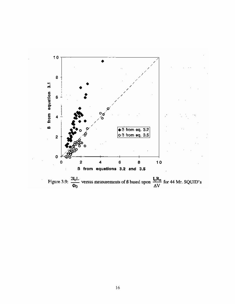
Figure 3.9 illustrates the differences between the Lβ ’s calculated using Equations 3.1, 3.2 and 3.5. As one can see from Figure 3.9, the method of calculating Lβ which takes into account the thermal effects agrees quite well with the inductive Lβ measurements. On the following page, we include a data sheet for your SQUID. You may wish to use it to enter your measurements on the SQUID. An interesting and important issue for SQUID applications is how the SQUID sensor varies with age. Summary of Basic Experiments By going through the previous set of experiments, you should have been able to observe the fundamental properties of Josephson junctions and SQUIDs and calculate the values of these key parameters:

16

17

• the critical current of the SQUID, IC ,

• the normal-state resistance, Rn ,

• the characteristic voltage of the SQUID, IC Rn ,

• the voltage modulation depth, ∆V,

• the inductance of the SQUID, L, and

• the Lβ value of the SQUID, using two methods.

18

Mr. SQUID Data Sheet

19

Part 2 : The AC Josephson Effect

Microwave-induced (Shapiro) Steps at 77K & h/e

Purpose and Discussion: The following discussion of the ac Josephson effect contains a fair amount of mathematical rigor in order to quantitatively explain the origin of the microwave-induced steps in the V-I curve of a Josephson junction. The current density (J) of a Josephson junction with a fixed dc voltage (V) across it oscillates according to the equation:

04J( ) J sin (0) eVtt

hπδ⎡ ⎤⎛ ⎞= − ⎜ ⎟⎢ ⎥⎝ ⎠⎣ ⎦

where e is the charge on an electron (1.602 x 1910− coulomb), δ(0) is the superconducting phase across the junction at time t=0, and h is Planck's constant (6.62 x 3410− J-s). This is called the AC Josephson Effect. This means that the current in the junction oscillates with a frequency of

2 4 V/heω πν π= = . A 1 µV DC voltage across a Josephson junction will cause the current to oscillate at ν = 4.83593420 x 810 Hz. Note that this formula contains neither materials parameters nor extrinsic quantities such as temperature. This formula holds for a niobium Josephson junction at 0.01K as well as the high-Tc grain-boundary Josephson junctions in your Mr. SQUID unit. The frequency (v) only depends on the ratio of twice the electronic charge, to Planck's constant. In fact, the National Institute of Standards (NIST) uses the AC Josephson Effect to set the standard for the "0fficial" value of the volt. As a practical matter, one cannot DC voltage bias a Josephson junction to a few microvolts, set a radio receiver next to it, and tune in to the radio frequency (RF) radiation emitted by the junc-tion. The main reason is that the impedance of free space is ~370Ω while the junction is usually much less than 1Ω. For this reason, the RF will stay in the junction rather than radiate away into free space. The AC Josephson Effect is usually observed by placing the DC voltage biased junction in an applied oscillating electric field. In this case, V → V(t), which alters the AC Josephson Effect equation to:

( )0

0

4J(t) = J sin (0)

t eV tdt

hπ

δ⎡ ⎤′⎛ ⎞

′−⎢ ⎥⎜ ⎟⎢ ⎥⎝ ⎠⎣ ⎦

∫ .

20

If 0 aV(t) = V V cos( )atω+ , then

( )00

4 4J(t) = J sin (0) sinaa

a

eV t eV th h

π πδ ωω

⎡ ⎤⎛ ⎞⎛ ⎞− −⎢ ⎥⎜ ⎟⎜ ⎟⎝ ⎠ ⎝ ⎠⎣ ⎦

.

The above equation can be expanded in a Fourier-Bessel series using the relations:

sin( sin ) ( )sin( )

cos( sin ) ( )cos( )

n

n

X B X n

X B X n

α α

α α

+∞

−∞

+∞

−∞

=

=

∑

∑

where, to avoid confusion with the current density J, the symbol Bn(X) has been used for the Bessel function of order n and argument X. The current density then becomes:

00

4 4J(t) = J sin (0)an a

a

eV eVB n th hπ πδ ωω

+∞

−∞

⎡ ⎤⎛ ⎞ ⎛ ⎞⎛ ⎞+ +⎜ ⎟ ⎢ ⎥⎜ ⎟⎜ ⎟⎝ ⎠⎝ ⎠⎝ ⎠ ⎣ ⎦

∑ ,

This equation is a sum of components at infinitely many frequencies, 04a

eVnh

πω + . In particular

when the frequency 04a

eVnh

πω + vanishes, so 04anh eVω π= − where 0, 1, 2,.....n = ± ± there will

be a component of the supercurrent density at zero frequency. A DC supercurrent will therefore be present in the junction whenever the DC voltage V0 across the junction has one of the values:

0 ( )4

ahV ne

ωπ

=

where n is any integer. These zero-frequency supercurrents correspond to the appearance of a DC Josephson effect at a non-zero voltage V0 across the junction when the junction is irradiated with electromagnetic radiation of frequency ωa. There will thus be a discontinuous shift in the DC current, with no change in the DC voltage across the junction. If one is sweeping out a V-I curve while applying an ac electric field to the Josephson junction, one will see a curve similar to the one which appears below. Such constant voltage steps (i.e. discontinuous shift in the AC current) in the V-I curve are called Shapiro steps. There are a number of ways to impress an AC voltage on Josephson junctions. The easiest way is to simply send microwaves (ν >1 GHz) into the cryogenic container holding the Josephson junction. Due to the high sensitivity of the Josephson junctions, even at very modest RF power levels a significant amount of radiation will couple into the junctions despite the large impedance mismatch between the junctions and free space. For this experiment you will need: • The DC SQUID & a dewar filled with liquid nitrogen • An oscilloscope

21

• A microwave source of known frequency, capable of operating between 1 and 10 GHz. Illustrated below is a procedure to couple microwaves (MW) from a generator into the SQUID dewar. For the illustration which follows, we used an HP83711B function generator which

can produce microwaves with frequencies in the range of 1 GHz to 20 GHz. Any microwave source that you can couple into the Mr. SQUID dewar should work. A coaxial cable is connected to the generator. The other end of the coaxial cable is devoid of a connector. Instead, approximately 2-3 cm of the coax cable's shield was removed to expose a 2-3 cm length of the center conductor, which acts as an antenna. If you do not have access to a microwave function generator, a microwave generator with a horn antennae may be used and pointed down into the dewar. Due to possible resonances and spurious microwave modes developing inside your Mr. SQUID dewar at specific frequencies, a generator with some frequency tuning will make this experiment easier to perform. A word of caution: Microwave radiation can be dangerous even at relatively low levels, es-pecially in the frequency range of this experiment, 1-10 GHz. For example, microwave ovens operate at –2.45 GHz where H20 is very strongly absorbing. The maximum safe level, as specified by the U.S. Government, for RF and MW radiation is 10 mW/cm 2 However, this is

22

23

higher than the maximum safe levels specified by many countries27, some of which have specified maximum safe levels as low as 0.01 mW/cm 2 . Read the instructions for your microwave generating equipment and follow ALL safety instructions. Set up your Mr. SQUID unit and cool it down with liquid nitrogen. Turn it on in the V-I mode. This is the only mode we will be using in this experiment. You will need to have a fairly clean V-I curve as illustrated below, free of flux trapping and RF interference.

Procedure for using a coaxial cable/microwave generator: Step 1. Once you have a clean V-I curve, reset the microwave generator to its lowest frequency setting or 1 GHz, whichever is higher. Slowly increase the amplitude on the microwave generator. At some point, you should see the V-I curve flatten out, with a complete disappearance of the su-percurrent. You may or may not see steps in the V-I curve before this point. The reason is that the Mr. SQUID dewar - coaxial cable combination acts as a complicated resonator with many modes. Many of these modes may couple with the SQUID junctions enough to exceed their critical currents, but do not couple with the junctions correctly to display the AC Josephson Effeet. 27 For example, Pethig states on page 235 that in the USA and UK, permissible microwave exposure levels are a maximum power density of l0 mW/cm2 and exposures should not exceed lmW/cm2 for a continuous period of less than 0.1 hour. In the Former Soviet Union, the limit is stated by Pethig as 0.0lmW/cm2 for one working day, and wearing protective equipment is required for exposures not to exceed lmW/cm2 for 20 minutes or 0.lmW/cm2 for 2 hours. Dielectric and Electrical Properties of Biological Materials by Ronald Pethig, (John Wiley and Sons, 1979)

24

Step 2. Once you have surpassed the critical current, back the amplitude back down until part (one half to one third) of the original supercurrent has returned. At this point, slowly change the frequency. Watch the V-I curve while you are doing this. Agaln, due to the various electromagnetic modes which can arise inside the squid dewar, not all frequencies will properly couple into the squid. Keep slowly varying the frequency until you see a symmetric pattern of steps in the V-I curve. Below is an illustration of the squid V-I curve from step 1 after tuning to 4.520 GHz, which shows two steps, one at about +1.9 divisions and one at about -1.9 divisions. Trouble-avoidance tip: If you cannot see any steps in the V-I curve after tuning the frequency up all the way, go back and repeat step 1 at a slightly higher frequency, then repeat step 2. Due to the spurious electromagnetic modes which form in the squid dewar due to the silver coating inside the glass dewar, getting the microwaves to couple properly can be somewhat of a "black art".

Determining e/h To determine the value of e/h, we need to measure the voltages at which the steps occur. From the trace shown above, we would place the steps at +9.25 µvolts and at –9.25 µvolts. (note: The vertical scale on the scope display is 50 mV per major division, which with the 10 4 gain of the squid controller, means the scale of the display is really 5 µV per major division). Since

0V4 2

a anh nhe eω νπ

= =

25

then

0

e h 2

anVν

=

As can be seen by comparing the oscilloscope trace immediately above with the Shapiro step illustration earlier, our steps correspond to the n = 1± steps. So for our data above:

9

14-6

0

e 4.52 10 Hz Hz2.44 10h 2V 2 x 9.25 x 10 V volt

a x xν= = = .

The "official" value of e/h is 2.4179671 x 1014 Hz/volt which means our measurement was good to about 0.8%. This relatively high level of accuracy using such a simple measurement is the reason the AC Josephson Effect is used by the National Institute of Standards. However, for us to claim that we made this measurement to this level of accuracy would be somewhat misleading. The reason is that if you look at the scope picture of the Shapiro steps above, the steps are not perfectiy flat, and show some rounding. This might be due to small fluc-tuations in the microwave generator frequency or they might also be due to thermal noise in the squid. Remember, although 77 K may seem cold to us, it is rather "hot" compared to the super-

conducting transition temperature of your squid C

77 K 0.85T

⎛ ⎞≈⎜ ⎟

⎝ ⎠. So there is some uncertainty

in the placement of the steps. The voltages at which the steps appear could be stated to be at 9.25 0.3 Vµ± . This uncertainty corresponds to an uncertainty in e/h of about 6%. So our value for e/h is ( ) 142.44 0.16 10 Hz/Vx± ,

as compared to the "official value" of 2.4179671 x 1014 Hz/V. One can increase the accuracy of this measurement by cooling the squid to reduce the thermal rounding of the steps, by stabilizing the microwave source so that its frequency does not fluctuate, and shielding the squid from RF interferences (other than the microwave source) which can also cause rounding of the steps. By doing all these things, the ratio of value for e/h has been determined to a large number of decimal places.28 Since ultra-stable frequency sources are relatively easy to build (e.g. atomic clocks), the U.S. National Institute of Standards (NIST) uses such time references along with the AC Josephson Effect to set the standard for the "official" value of the volt. 28 W.H. Parker, B.N. Taykor, and D.N. Langenburg, Phys. Rev. Letters 18, 287 (1967)

26

APPENDIX : SQUID Chip (nominal): System Specifications: SQUID 4-probe resistance (using Mr. SQUID Electronics): 300-400 Ω @ 295K 0.2-0.5 Ω @ 77K @ high currents 0 Ω @ 77K @ low current Critical current (minimum): 5 µA @ 77K Magnetic field modulation (minimum): 1 µV @ 77K Internal & external coil mutual inductance to the SQUID (M): ~43 pH SQUID self inductance (L): ~93 pH Internal & external coil resistance: 22 Ω @ 295K 18 Ω @ 77K SQUID Noise Floor: Mr. SQUID electronics limited at 3

010 / Hz− Φ∼ @ 100Hz

SQUID intrinsically limited at 4010 / Hz− Φ∼ @ 100Hz @ 77K

SQUID washer dimensions: 250 µm x 250 µm outer body 20 µm x 20 µm hole 155 µm slot, 2 µm wide