Summary of previous lesson

• Janzen-Connol hypothesis; explanation of why diseases lead to spatial heterogeneity

• Diseases also lead to heterogeneity or changes through time– Driving succession– The Red Queen Hypothesis: selection pressure will increase number of resistant plant genotypes

• Co-evolution: pathogen increase virulence in short term, but in long term balance between host and pathogen

• Density dependance

Disease and competition

• Competition normally is conducive to increased rates of disease: limited resources weaken hosts, contagion is easier

• Pathogens can actually cryptically drive competition, by disproportionally affecting one species and favoring another

Janzen-Connol

• Regeneration near parents more at risk of becoming infected by disease because of proximity to mother (Botryosphaeria, Phytophthora spp.). Maintains spatial heterogeneity in tropical forests

• Effects are difficult to measure if there is little host diversity, not enough host-specificity on the pathogen side, and if periodic disturbances play an important role in the life of the ecosystem

Diseases and succession

• Soil feedbacks; normally it’s negative. Plants growing in their own soil repeatedly have higher mortality rate. This is the main reason for agricultural rotations and in natural systems ensures a trajectory towards maintaining diversity

• Phellinus weirii takes out Douglas fir and hemlock leaving room for alder

The red queen hypothesis

• Coevolutionary arm race• Dependent on:

– Generation time has a direct effect on rates of evolutionary change

– Genetic variability available– Rates of outcrossing (Hardy-weinberg equilibrium)

– Metapopulation structure

Diseases as strong forces in plant

evolution• Selection pressure• Co-evolutionary processes

– Conceptual: processes potentially leading to a balance between different ecosystem components

– How to measure it: parallel evolution of host and pathogen

• Rapid generation time of pathogens. Reticulated evolution very likely. Pathogens will be selected for INCREASED virulence

• In the short/medium term with long lived trees a pathogen is likely to increase its virulence

• In long term, selection pressure should result in widespread resistance among the host

More details on:

• How to differentiate linear from reticulate evolution: comparative studies on topology of phylogenetic trees will show potential for horizontal transfers. Phylogenetic analysis neeeded to confirm horizontal transmission

Phylogenetic Phylogenetic relationships relationships within the within the HeterobasidionHeterobasidion complexcomplex

Het INSULARE

True Fir EUROPE

Spruce EUROPE

True Fir NAMERICA

Pine EUROPE

Pine NAMERICA

0.05 substitutions/site

NJ

Fir-SpruceFir-Spruce

Pine EuropePine Europe

Pine N.Am.Pine N.Am.

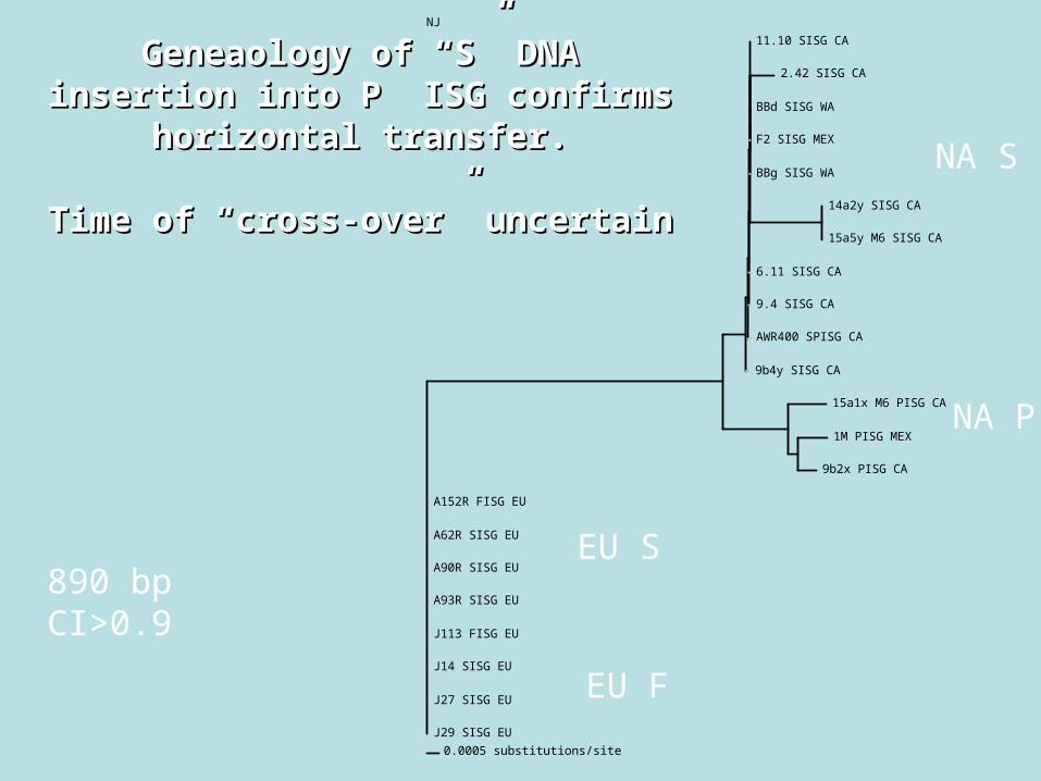
Geneaology of “S” DNA Geneaology of “S” DNA insertion into P ISG confirms insertion into P ISG confirms

horizontal transfer.horizontal transfer.

Time of “cross-over” uncertainTime of “cross-over” uncertain

11.10 SISG CA

2.42 SISG CA

BBd SISG WA

F2 SISG MEX

BBg SISG WA

14a2y SISG CA

15a5y M6 SISG CA

6.11 SISG CA

9.4 SISG CA

AWR400 SPISG CA

9b4y SISG CA

15a1x M6 PISG CA

1M PISG MEX

9b2x PISG CA

A152R FISG EU

A62R SISG EU

A90R SISG EU

A93R SISG EU

J113 FISG EU

J14 SISG EU

J27 SISG EU

J29 SISG EU

0.0005 substitutions/site

NJ

890 bpCI>0.9

NA S

NA P

EU S

EU F

Complexity of forest diseases

• At the individual tree level: 3 dimensional

• At the landscape level” host diversity, microclimates, etc.

• At the temporal level

Complexity of forest diseases

• Primary vs. secondary• Introduced vs. native• Air-dispersed vs. splash-dispersed, vs. animal vectored

• Root disease vs. stem. vs. wilt, foliar

• Systemic or localized

Stem cankerStem cankeron coast live oakon coast live oak

Progression of cankersProgression of cankers

Older canker with dry seepOlder canker with dry seepHypoxylonHypoxylon, a secondary , a secondary sapwood decayer will appearsapwood decayer will appear

Root disease center in true fir caused by Root disease center in true fir caused by H. annosumH. annosum

HOST-SPECIFICITY

• Biological species• Reproductively isolated• Measurable differential: size of structures

• Gene-for-gene defense model• Sympatric speciation: Heterobasidion, Armillaria, Sphaeropsis, Phellinus, Fusarium forma speciales

Phylogenetic Phylogenetic relationships relationships within the within the HeterobasidionHeterobasidion complexcomplex

Het INSULARE

True Fir EUROPE

Spruce EUROPE

True Fir NAMERICA

Pine EUROPE

Pine NAMERICA

0.05 substitutions/site

NJ

Fir-SpruceFir-Spruce

Pine EuropePine Europe

Pine N.Am.Pine N.Am.

Recognition of self vs. non self

• Intersterility genes: maintain species gene pool. Homogenic system

• Mating genes: recognition of “other” to allow for recombination. Heterogenic system

• Somatic compatibility: protection of the individual.

Recognition of self vs. non self

• What are the chances two different individuals will have the same set of VC alleles?

• Probability calculation (multiply frequency of each allele)

• More powerful the larger the number of loci

• …and the larger the number of alleles per locus

INTERSTERILITY

• If a species has arisen, it must have some adaptive advantages that should not be watered down by mixing with other species

• Will allow mating to happen only if individuals recognized as belonging to the same species

• Plus alleles at one of 5 loci (S P V1 V2 V3)

MATING

• Two haploids need to fuse to form n+n

• Sex needs to increase diversity: need different alleles for mating to occur

• Selection for equal representation of many different mating alleles

SEX

• Ability to recombine and adapt• Definition of population and metapopulation

• Different evolutionary model• Why sex? Clonal reproductive approach can be very effective among pathogens

Long branches in Long branches in between groups between groups suggests no sex is suggests no sex is occurring in occurring in between groupsbetween groups

Het INSULARE

True Fir EUROPE

Spruce EUROPE

True Fir NAMERICA

Pine EUROPE

Pine NAMERICA

0.05 substitutions/site

NJ

Fir-SpruceFir-Spruce

Pine EuropePine Europe

Pine N.Am.Pine N.Am.

Small branches within a clade Small branches within a clade indicate sexual reproduction indicate sexual reproduction is ongoing within that group is ongoing within that group

of individualsof individuals

11.10 SISG CA

2.42 SISG CA

BBd SISG WA

F2 SISG MEX

BBg SISG WA

14a2y SISG CA

15a5y M6 SISG CA

6.11 SISG CA

9.4 SISG CA

AWR400 SPISG CA

9b4y SISG CA

15a1x M6 PISG CA

1M PISG MEX

9b2x PISG CA

A152R FISG EU

A62R SISG EU

A90R SISG EU

A93R SISG EU

J113 FISG EU

J14 SISG EU

J27 SISG EU

J29 SISG EU

0.0005 substitutions/site

NJ

890 bpCI>0.9

NA S

NA P

EU S

EU F

Index of association

Ia= if same alleles are associated too much as opposed to random, it

means sex is not occurring

Association among alleles calculated and compared

to simulated random distribution

SOMATIC COMPATIBILITY

• Fungi are territorial for two reasons– Selfish– Do not want to become infected

• If haploids it is a benefit to mate with other, but then the n+n wants to keep all other genotypes out

• Only if all alleles are the same there will be fusion of hyphae

• If most alleles are the same, but not all, fusion only temporary

The biology of the organism drives an

epidemic• Autoinfection vs. alloinfection• Primary spread=by spores• Secondary spread=vegetative, clonal spread, same genotype . Completely different scales (from small to gigantic)

Coriolus

HeterobasidionArmillariaPhellinus

OUR ABILITY TO:

• Differentiate among different individuals (genotypes)

• Determine gene flow among different areas

• Determine allelic distribution in an area

WILL ALLOW US TO DETERMINE:

• How often primary infection occurs or is disease mostly chronic

• How far can the pathogen move on its own

• Is the organism reproducing sexually? is the source of infection local or does it need input from the outside

Evolution and Population genetics

• Positively selected genes:……• Negatively selected genes……• Neutral genes: normally population genetics demands loci used are neutral

• Loci under balancing selection…..

Evolution and Population genetics

• Positively selected genes:……• Negatively selected genes……• Neutral genes: normally population genetics demands loci used are neutral

• Loci under balancing selection…..

Evolutionary history

• Darwininan vertical evolutionray models

• Horizontal, reticulated models..

Phylogenetic Phylogenetic relationships relationships within the within the HeterobasidionHeterobasidion complexcomplex

Het INSULARE

True Fir EUROPE

Spruce EUROPE

True Fir NAMERICA

Pine EUROPE

Pine NAMERICA

0.05 substitutions/site

NJ

Fir-SpruceFir-Spruce

Pine EuropePine Europe

Pine N.Am.Pine N.Am.

Geneaology of “S” DNA Geneaology of “S” DNA insertion into P ISG confirms insertion into P ISG confirms

horizontal transfer.horizontal transfer.

Time of “cross-over” uncertainTime of “cross-over” uncertain

11.10 SISG CA

2.42 SISG CA

BBd SISG WA

F2 SISG MEX

BBg SISG WA

14a2y SISG CA

15a5y M6 SISG CA

6.11 SISG CA

9.4 SISG CA

AWR400 SPISG CA

9b4y SISG CA

15a1x M6 PISG CA

1M PISG MEX

9b2x PISG CA

A152R FISG EU

A62R SISG EU

A90R SISG EU

A93R SISG EU

J113 FISG EU

J14 SISG EU

J27 SISG EU

J29 SISG EU

0.0005 substitutions/site

NJ

890 bpCI>0.9

NA S

NA P

EU S

EU F

Because of complications such as:• Reticulation• Gene homogeneization…(Gene duplication)

• Need to make inferences based on multiple genes

• Multilocus analysis also makes it possible to differentiate between sex and lack of sex (Ia=index of association)

Basic definitions again

• Locus• Allele• Dominant vs. codominant marker– RAPDS– AFLPs

How to get multiple loci?

• Random genomic markers:– RAPDS– Total genome RFLPS (mostly dominant)– AFLPS

• Microsatellites• SNPs• Multiple specific loci

– SSCP– RFLP– Sequence information

Watch out for linked alleles (basically you are looking at the same thing!)

Sequence information

• Codominant• Molecules have different rates of mutation, different molecules may be more appropriate for different questions

• 3rd base mutation• Intron vs. exon• Secondary tertiary structure limits• Homoplasy

Sequence information

• Multiple gene genealogies=definitive phylogeny

• Need to ensure gene histories are comparable” partition of homogeneity test

• Need to use unlinked loci

QuickTime™ and aTIFF (Uncompressed) decompressor

are needed to see this picture.

Thermalcycler

DNA template

Forward primer Reverse primer

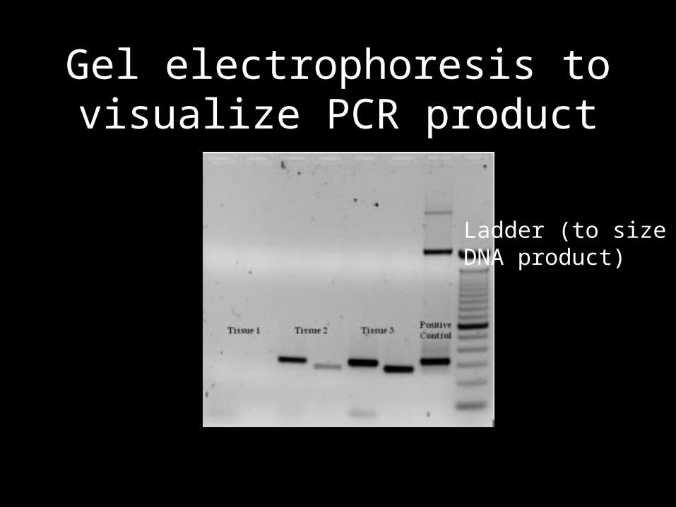
Gel electrophoresis to visualize PCR product

Ladder (to sizeDNA product)

From DNA to genetic information (alleles are distinct DNA sequences)

• Presence or absence of a specific PCR amplicon (size based/ specificity of primers)

• Differerentiate through:– Sequencing– Restriction endonuclease– Single strand conformation polymorphism

Presence absence of amplicon

• AAAGGGTTTCCCNNNNNNNNN• CCCGGGTTTAAANNNNNNNNN

AAAGGGTTTCCC (primer)

Presence absence of amplicon

• AAAGGGTTTCCCNNNNNNNNN• CCCGGGTTTAAANNNNNNNNN

AAAGGGTTTCCC (primer)

RAPDS use short primers but not too

short• Need to scan the genome• Need to be “readable”• 10mers do the job (unfortunately annealing temperature is pretty low and a lot of priming errors cause variability in data)

RAPDS use short primers but not too

short• Need to scan the genome• Need to be “readable”• 10mers do the job (unfortunately annealing temperature is pretty low and a lot of priming errors cause variability in data)

RAPDS can also be obtained with

Arbitrary Primed PCR• Use longer primers• Use less stringent annealing conditions

• Less variability in results

Result: series of bands that are present

or absent (1/0)

Root disease center in true fir caused by Root disease center in true fir caused by H. annosumH. annosum

Ponderosa pine Incense cedar

Yosemite Lodge 1975 Root disease centers outlined

Yosemite Lodge 1997 Root disease centers outlined

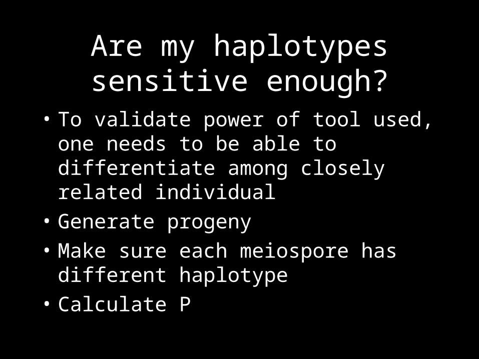
Are my haplotypes sensitive enough?

• To validate power of tool used, one needs to be able to differentiate among closely related individual

• Generate progeny• Make sure each meiospore has different haplotype

• Calculate P

RAPD combination1 2

• 1010101010

• 1010101010

• 1010101010

• 1010101010• 1010000000

• 1011101010

• 1010111010

• 1010001010

• 1011001010• 1011110101

Conclusions

• Only one RAPD combo is sensitive enough to differentiate 4 half-sibs (in white)

• Mendelian inheritance?• By analysis of all haplotypes it is apparent that two markers are always cosegregating, one of the two should be removed

AFLP

• Amplified Fragment Length Polymorphisms

• Dominant marker• Scans the entire genome like RAPDs• More reliable because it uses longer PCR primers less likely to mismatch

• Priming sites are a construct of the sequence in the organism and a piece of synthesized DNA

How are AFLPs generated?

• AGGTCGCTAAAATTTT (restriction site in red)

• AGGTCG CTAAATTT• Synthetic DNA piece ligated

– NNNNNNNNNNNNNNCTAAATTTTT

• Created a new PCR priming site– NNNNNNNNNNNNNNCTAAATTTTT

• Every time two PCR priming sitea are within 400-1600 bp you obtain amplification

Dealing with dominant anonymous multilocus

markers• Need to use large numbers (linkage)

• Repeatability• Graph distribution of distances

• Calculate distance using Jaccard’s similarity index

Jaccard’s

• Only 1-1 and 1-0 count, 0-0 do not count

101001110010111001000

Jaccard’s

• Only 1-1 and 1-0 count, 0-0 do not count

A: 1010011 AB= 0.6 0.4 (1-AB)

B: 1001011 BC=0.5 0.5C: 1001000 AC=0.2 0.8

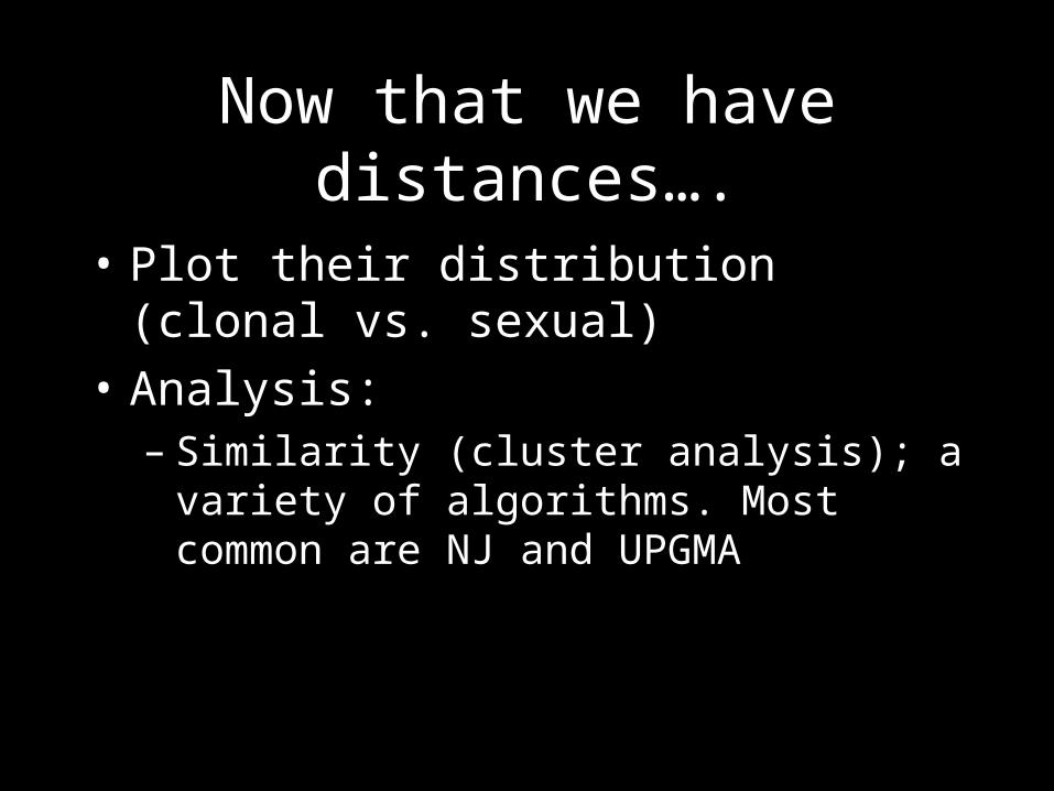
Now that we have distances….

• Plot their distribution (clonal vs. sexual)

Now that we have distances….

• Plot their distribution (clonal vs. sexual)

• Analysis: – Similarity (cluster analysis); a variety of algorithms. Most common are NJ and UPGMA

Now that we have distances….

• Plot their distribution (clonal vs. sexual)

• Analysis: – Similarity (cluster analysis); a variety of algorithms. Most common are NJ and UPGMA

– AMOVA; requires a priori grouping

AMOVA groupings

• Individual• Population• Region

AMOVA: partitions molecular variance amongst a priori defined groupings

Now that we have distances….

• Plot their distribution (clonal vs. sexual)

• Analysis: – Similarity (cluster analysis); a variety of algorithms. Most common are NJ and UPGMA

– AMOVA; requires a priori grouping– Discriminant, canonical analysis

Results: Jaccard similarity coefficients

0.3

0.90 0.92 0.94 0.96 0.98 1.00

00.10.2

0.40.50.60.7

Coefficient

Fre

quen

cy

P. nemorosa

P. pseudosyringae: U.S. and E.U.

0.3

Coefficient0.90 0.92 0.94 0.96 0.98 1.00

00.10.2

0.40.50.60.7

Fre

quen

cy

Fre

quen

cy

0.9 0.91 0.92 0.93 0.94 0.95 0.96 0.97 0.98 0.99

Pp U.S.

Pp E.U.

0.0

0.1

0.2

0.3

0.4

0.5

0.6

Jaccard coefficient of similarity

0.7

P. pseudosyringae genetic similarity patterns are

different in U.S. and E.U.

0.1

4175A

p72

p39

p91

1050

p7

2502

p51

2055.2

2146.1

5104

4083.1

2512

2510

2501

2500

2204

2201

2162.1

2155.3

2140.2

2140.1

2134.1

2059.2

2052.2

HCT4

MWT5

p114

p113

p61

p59

p52

p44

p38

p37

p13

p16

2059.4

p115

2156.1

HCT7

p106

P. nemorosa

P. ilicisP. pseudosyringae

Results: Results: P. nemorosaP. nemorosa

Results: Results: P. pseudosyringaeP. pseudosyringae

0.1

4175A2055.2p44

FC2DFC2E

GEROR4 FC1B

FCHHDFCHHCFC1A

p80FAGGIO 2FAGGIO 1FCHHBFCHHAFC2FFC2CFC1FFC1DFC1Cp83p40

BU9715 p50

p94p92

p88p90

p56Bp45

p41p72p84p85p86p87p93p96p39p118p97p81p76p73p70p69p62p55p54

HELA2HELA 1

P. nemorosaP. ilicis

P. pseudosyringae

= E.U. isolate

Now that we have distances….

• Plot their distribution (clonal vs. sexual)

• Analysis: – Similarity (cluster analysis); a variety of algorithms. Most common are NJ and UPGMA

– AMOVA; requires a priori grouping– Discriminant, canonical analysis – Frequency: does allele frequency match expected (hardy weinberg), F or Wright’s statistsis

The “scale” of disease

• Dispersal gradients dependent on propagule size, resilience, ability to dessicate, NOTE: not linear

• Important interaction with environment, habitat, and niche availability. Examples: Heterobasidion in Western Alps, Matsutake mushrooms that offer example of habitat tracking

• Scale of dispersal (implicitely correlated to metapopulation structure)---

The “scale” of disease

• Dispersal gradients dependent on propagule size, resilience, ability to dessicate, NOTE: not linear

• Important interaction with environment, habitat, and niche availability. Examples: Heterobasidion in Western Alps, Matsutake mushrooms that offer example of habitat tracking

• Scale of dispersal (implicitely correlated to metapopulation structure)---

Have we sampled enough?

• Resampling approaches• Saturation curves

– A total of 30 polymorphic alleles– Our sample is either 10 or 20– Calculate whether each new sample is characterized by new alleles

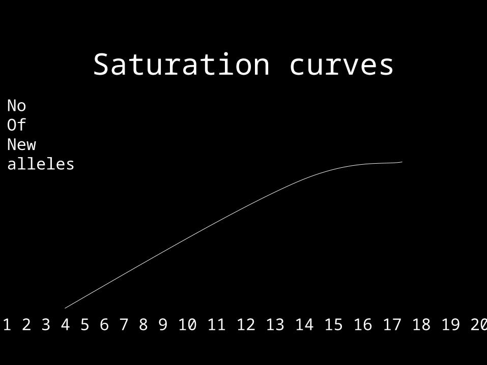
Saturation curves

1 2 3 4 5 6 7 8 9 10 11 12 13 14 15 16 17 18 19 20

NoOf Newalleles

If we have codominant markers how many do I

need• IDENTITY tests = probability calculation based on allele frequency… Multiplication of frequencies of alleles

• 10 alleles at locus 1 P1=0.1• 5 alleles at locus 2 P2=0,2• Total P= P1*P2=0.02

White mangroves:Corioloposis caperata

White mangroves:Corioloposis caperata

Coco Solo Mananti Ponsok DavidCoco Solo 0Mananti 237 0Ponsok 273 60 0David 307 89 113 0

Distances between study sites

Coriolopsis caperataCoriolopsis caperata on on Laguncularia racemosaLaguncularia racemosa

Forest fragmentation can lead to loss of gene flow among previously contiguous populations. The negative repercussions of such genetic isolation should most severely affect highly specialized organisms such as some plant-parasitic fungi.

AFLP study on single spores

Site # of isolates # of loci % fixed alleles

Coco Solo 11 113 2.6

David 14 104 3.7

Bocas 18 92 15.04

Distances =PhiST between pairs ofpopulations. Above diagonal is the ProbabilityRandom distance > Observed distance (1000iterations).

Coco Solo Bocas David

Coco Solo 0.000 0.000 0.000

Bocas 0.2083 0.000 0.000

David 0.1109 0.2533 0.000

Using DNA sequences

• Obtain sequence• Align sequences, number of parsimony informative sites

• Gap handling• Picking sequences (order)• Analyze sequences (similarity/parsimony/exhaustive/bayesian

• Analyze output; CI, HI Bootstrap/decay indices

Using DNA sequences

• Testing alternative trees: kashino hasegawa

• Molecular clock• Outgroup• Spatial correlation (Mantel)

• Networks and coalescence approaches

QuickTime™ and aTIFF (LZW) decompressor

are needed to see this picture.

Pacifico

Caribe

From Garbelotto and Chapela, From Garbelotto and Chapela, Evolution and biogeography of Evolution and biogeography of

matsutakesmatsutakes

Biodiversity within speciesBiodiversity within speciesas significant as betweenas significant as betweenspeciesspecies