Spiky Strings and Giant Magnons on S5

M. Kruczenski

Purdue University

Based on: hep-th/0607044(Russo, Tseytlin, M.K.)

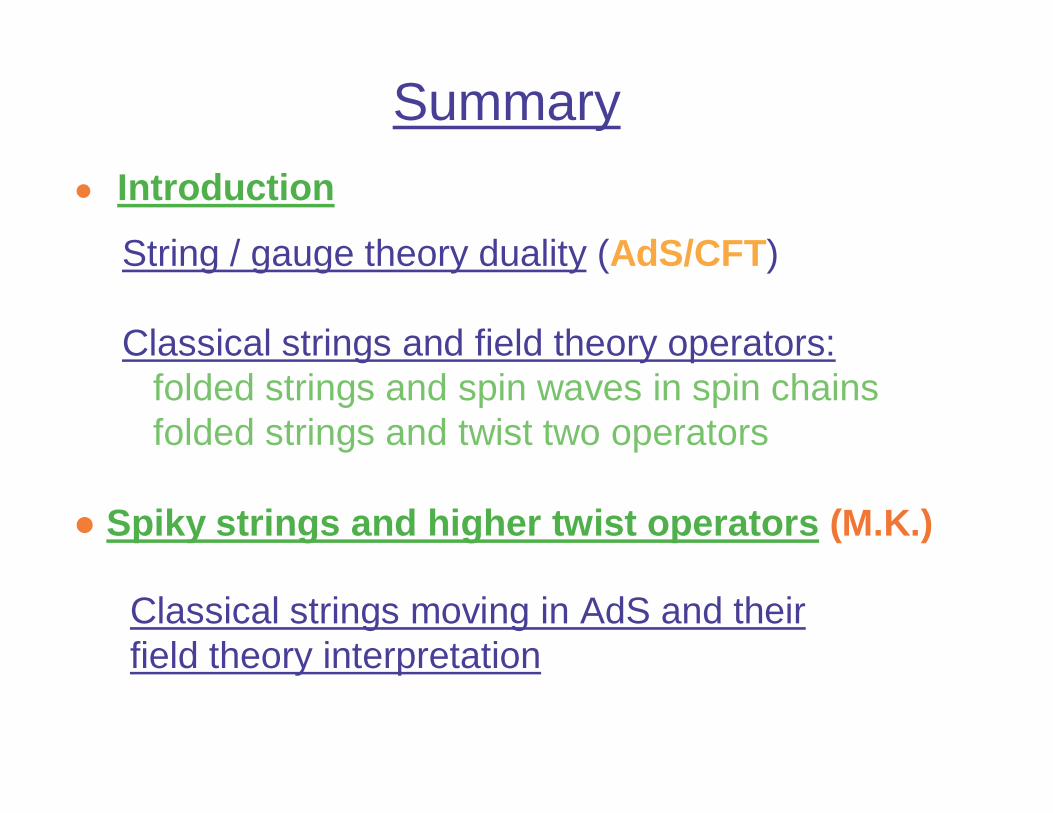
Summary

Introduction

String / gauge theory duality (AdS/CFT )

Classical strings and field theory operators:folded strings and spin waves in spin chainsfolded strings and twist two operators

Spiky strings and higher twist operators (M.K.)

Classical strings moving in AdS and theirfield theory interpretation

Spin chain interpretation of the giant magnon(Hofman-Maldacena)

More generic solutions: Spiky strings and giant magnons on S5

(Russo, Tseytlin, M.K.)

Conclusions

Spiky strings on a sphere and giant magnon limit(Ryang, Hofman-Maldacena)

Other solutions on S 2 (work in prog. w/ R.Ishizeki )

String/gauge theory duality: Large N limit (‘t Hooft)

mesons

String picture

, , ...

Quark model

Fund. strings

( Susy, 10d, Q.G. )

QCD [ SU(3) ]

Large N-limit [SU(N)]

Effective strings

q q

Strong coupling

q q

Lowest order: sum of planar diagrams (infinite number)

N g N fixedYM→ ∞ =, λ 2More precisely: (‘t Hooft coupl.)

AdS/CFT correspondence (Maldacena)

Gives a precise example of the relation betweenstrings and gauge theory.

Gauge theory

N = 4 SYM SU(N) on R4

A , i, a

Operators w/ conf. dim.

String theory

IIB on AdS5xS5

radius RString states w/ ∆ E

R=

∆

g g R l g Ns YM s YM= =2 2 1 4; / ( ) /

N g NYM→ ∞ =, λ 2 fixedlarge string th.small field th.

Can we make the map between string and gaugetheory precise?

It can be done in particular cases.

Take two scalars X = 1+ i 2 ; Y= 3 + i 4

O = Tr(XX…Y..Y…X) , J1 X’s , J2 Y’s, J1+J2 large

Compute 1-loop conformal dimension of O , or equiv.compute energy of a bound state of J1 particles of type X and J2 of type Y (but on a three sphere)

R4 S3xRE

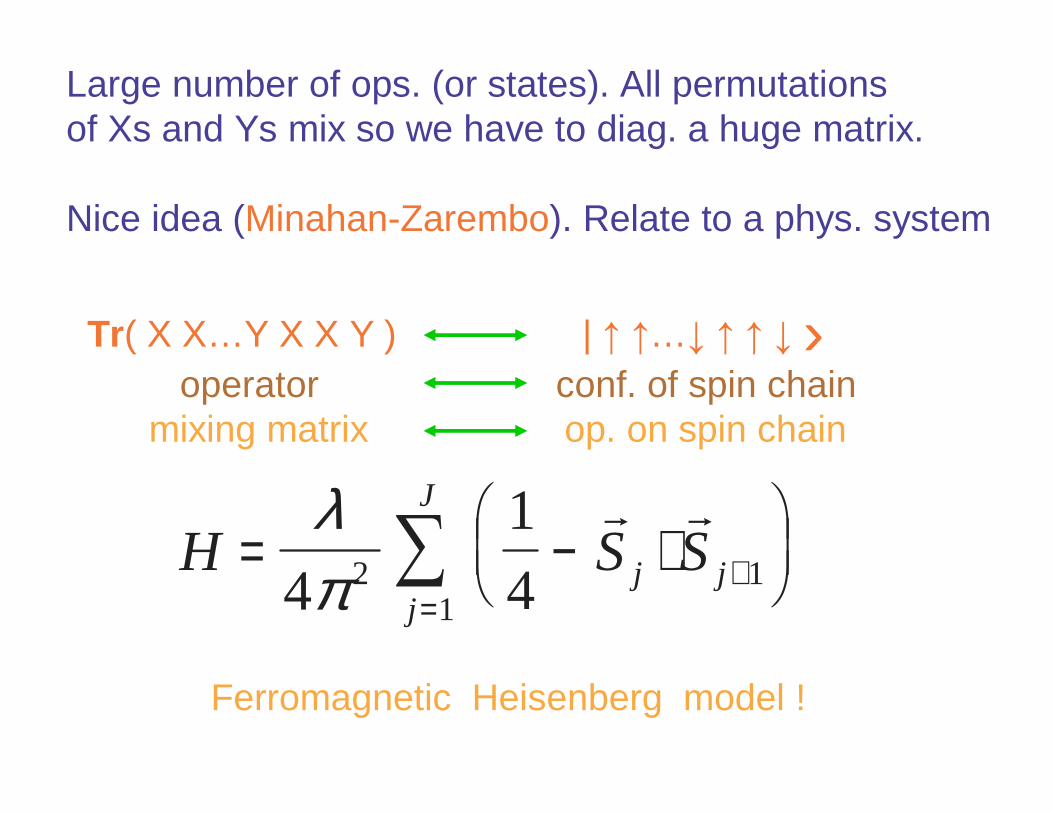
Large number of ops. (or states). All permutations of Xs and Ys mix so we have to diag. a huge matrix.

Nice idea (Minahan-Zarembo). Relate to a phys. system

Tr( X X…Y X X Y ) | … ›operator conf. of spin chain

mixing matrix op. on spin chain

Ferromagnetic Heisenberg model !

H S Sj jj

J

= − ⋅

+

=∑

λπ4

1

42 11

r r

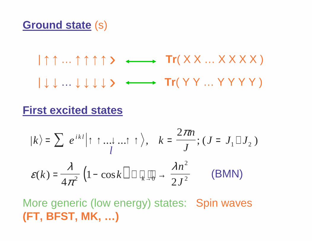
Ground state (s)

| … › Tr( X X … X X X X )

| … › Tr( Y Y … Y Y Y Y )

First excited states

More generic (low energy) states: Spin waves(FT, BFST, MK, …)

( )

| ... ... , ; ( )

( ) cos

k e kn

JJ J J

k kn

J

i k l

k

= ↑ ↑ ↓ ↑ ↑ = = +

= − →

∑

→

2

41

2

1 2

2 0

2

2

π

ελπ

λl

(BMN)

Other states , e.g. with J1=J2

Spin waves of long wave-length have low energy andare described by an effective action in terms of two angles , : direction in which the spin points.

Taking J large with /J2 fixed: classical solutionsMoreover, this action agrees with the action of a string moving fast on S5 .What about the case k ~ 1 ?

[ ]S J d dJeff . cos ( ) sin ( )= − − +

∫1

2 32 22 2 2σ τ θ ∂ φ

λπ

∂ θ θ ∂ φτ σ σ

Since ( , ) is interpreted as the position of the string

we get the shape of the string from ‹ S ›(σ)

Examples

| … ›point-like

( , )

Folded string

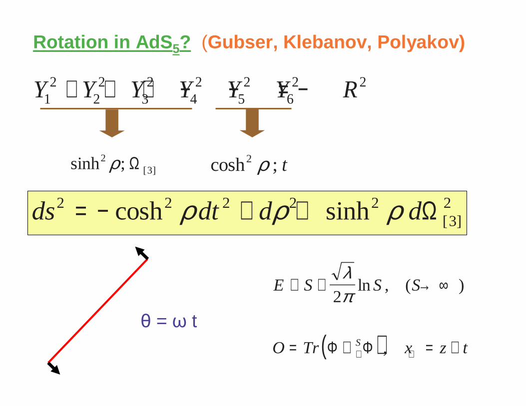
Rotation in AdS 5? (Gubser, Klebanov, Polyakov)

Y Y Y Y Y Y R12

22

32

42

52

62 2+ + + − − = −

sinh ; [ ]2

3ρ Ω cosh ;2 ρ t

ds dt d d2 2 2 2 23

2= − + +cosh sinh [ ]ρ ρ ρ Ω

( )

E S S S

O Tr x z tS

≅ + → ∞

= ∇ = ++ +

λπ2

ln , ( )

,Φ Φ= t

Verification using Wilson loops (MK, Makeenko)

The anomalous dimensions of twist two operators can also be computed by using the cusp anomaly of light-like Wilson loops (Korchemsky and Marchesini ).

In AdS/CFT Wilson loops can be computed using surfaces of minimal area in AdS5 (Maldacena, Rey, Yee )

z

The result agrees with the rotating string calculation.

Generalization to higher twist operators (MK)

( )O TrnS n S n S n S n

[ ]/ / / /= ∇ ∇ ∇ ∇+ + + +Φ Φ Φ ΦK( )O Tr S

[ ]2 = ∇ +Φ Φ

x A n A n

y A n A n

= − + −= − + −

+ −

+ −

cos[( ) ] ( ) cos[ ]

sin[( ) ] ( ) sin [ ]

1 1

1 1

σ σσ σ

In flat space such solutions are easily found in conf. gauge

Spiky strings in AdS:

( )

E Sn

S S

O Tr S n S n S n S n

≅ +

→ ∞

= ∇ ∇ ∇ ∇+ + + +

2 2

λπ ln , ( )

/ / / /Φ Φ Φ ΦK

S dt dtjj

j j

j

= − − +−

∑∫ ∑∫

+λπ ρ θ

λπ ρ

θ θ2

2 18

421 1

2 1(cosh )& ln sin

–2

–1

0

1

2

–2 –1 1 2

–2

–1

0

1

2

–2 –1 1 2

Spiky strings on a sphere: (Ryang )

Similar solutions exist for strings rotating on a sphere:

(top view)

The metric is:

We use the ansatz:And solve for . Field theory interpretation?

ds dt d d2 2 2 2 2= − + +θ θ ϕsin

t = = + =κτ ϕ ωτ σ θ θ σ, , ( )θ σ( )

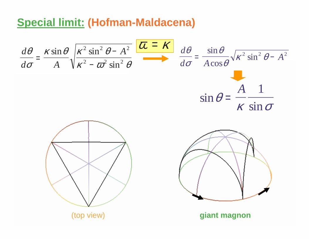
Special limit: (Hofman-Maldacena)

d

d A

Aθσ

κ θ κ θκ ω θ

=−

−sin sin

sin

2 2 2

2 2 2

ω κ= d

d AA

θσ

θθ κ θ= −

sin

cossin2 2 2

sinsin

θ κ σ=A 1

(top view) giant magnon

The energy and angular momentum of the giant magnonsolution diverge. However their difference is finite:

E JA d

A

− = =

= =

∫λπ κ

σσ

λπ

ϕ

ϕκ ϕ

2 2

2

2sinsin

cos ,

∆

∆∆ Angular distance between spikes

E J− = + ≅> >

+ < <

12

21

12 2

1

22

22

λπ

ϕλ

πϕ

λ

λπ

ϕλ

sin

sin ,

sin ,

∆∆

∆

Interpolating expression:

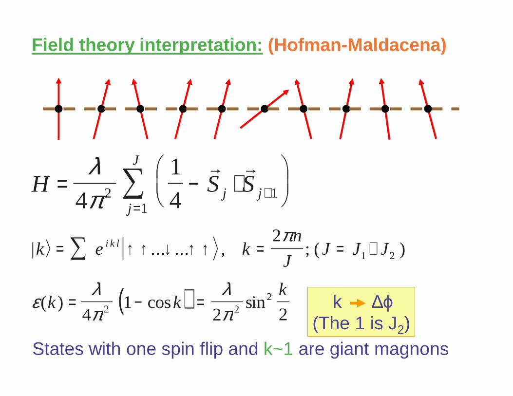
Field theory interpretation: (Hofman-Maldacena)

H S Sj jj

J

= − ⋅

+

=∑

λπ4

1

42 11

r r

( )

| ... ... , ; ( )

( ) cos sin

k e kn

JJ J J

k kk

i k l= ↑ ↑ ↓ ↑ ↑ = = +

= − =

∑2

41

2 2

1 2

2 22

π

ελπ

λπ

k ∆ϕ(The 1 is J2)

States with one spin flip and k~1 are giant magnons

More spin flips: (Dorey, Chen-Dorey-Okamura)

In the string side there are solutions with anotherangular momentum J2. The energy is given by:

E J J JJ

− = + ≅ + < <1 22

22

22

22

2 2 21

λπ

ϕ λπ

ϕλsin sin ,

∆ ∆

Justifies interpolating formula for J2=1

In the spin chain, if we flip a number J2 of spinsthere is a bound state with energy:

ελπ( ) sink

J

k=

2 222

2 k ∆ϕ(J2 is absorbed in J)

More general solutions: (Russo, Tseytlin, MK)

Strategy: We generalize the spiky string solutionand then take the giant magnon limit.

In flat space:x A n A n

y A n A n

= − + −= − + −

+ −

+ −

cos[( ) ] ( ) cos[ ]

sin[( ) ] ( ) sin [ ]

1 1

1 1

σ σσ σ

Consider txS5: ds dt dX d X X Xa aa

a aa

2 2

1

3

1

3

1= − + == =∑ ∑,

namely: x iy X x ei+ = = = +( ) ,ξ ξ α σ βτωτ

Use similar ansatz:

X x e r ea ai

ai ia a a= = +( ) ( ) ( )ξ ξω τ µ ξ ω τ

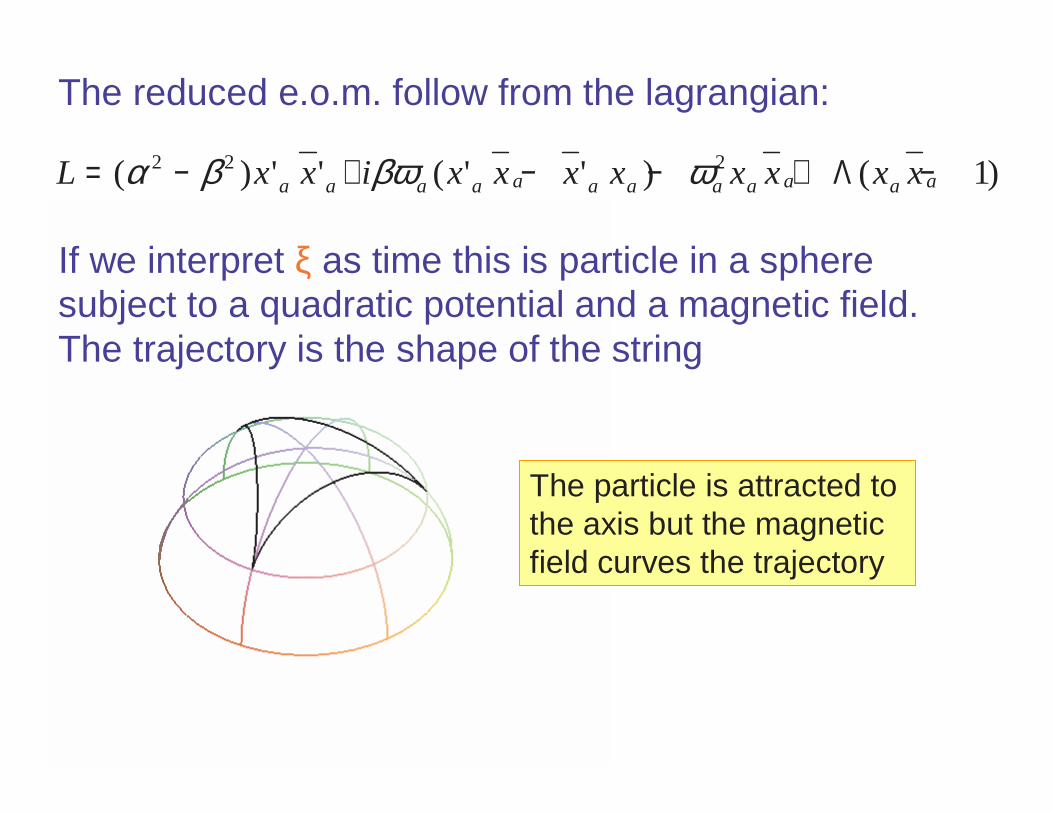
The reduced e.o.m. follow from the lagrangian:

L x x i x x x x x x x xa a a a a a a a a a a a= − + − − + −( ) ' ' ( ' ' ) ( )α β βω ω2 2 2 1Λ

If we interpret ξ as time this is particle in a sphere subject to a quadratic potential and a magnetic field.The trajectory is the shape of the string

The particle is attracted to the axis but the magnetic field curves the trajectory

Using the polar parameterization we get:

L rC

rr r

C

rx r e

aa

aa a a

aa

aa a a

i a

= − −−

−−

+ −

=−

+

=

( ) '( ) ( )

( )

'( )

,

α βα β

αα β

ω

µα β

βω µ

2 2 22 2

2

2

2

2 22 2 2

2 2

2

2

11

1

Λ

Constraints: ω βκα βα β

κa aC H+ = =+−

22 2

2 220 ,

Three ang. momenta: J dC

raa

a a=−

+−

∫ ξ

βα α β

αα β

ω( ) ( )2 2 2 2

2

Corresponding to phase rotations of x1,2,3

Solutions:

One angular momentum:

x3=0, x2 real (µ2=0), r12+r2

2=1, one variable.

Two angular momenta:

x3=0, r12+r2

2=1, one variable

Since only one variable we solve them usingconservation of H. Reproduced Ryang, Hofman-Maldacena and Chen-Dorey-Okamura

Three angular momenta: r12+r2

2+r32=1, r1,2

Therefore the three angular momenta case is the first “non-trivial” and requires more effort.It turns that this system is integrable as shown long ago by Neumann, Rosochatius and more recently by Moser.

Can be solved by doing a change of variables to ζ+, ζ−

raa a

a ba b

22 2

2 2=

− −−

+ −

≠∏

( )( )

( )

ζ ω ζ ωω ω

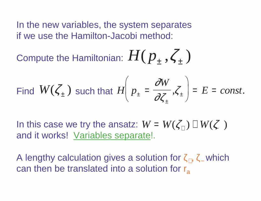
In the new variables, the system separatesif we use the Hamilton-Jacobi method:

Compute the Hamiltonian:

Find such that

In this case we try the ansatz: and it works! Variables separate!.

A lengthy calculation gives a solution for ζ+, ζ− which can then be translated into a solution for ra

H p( , )± ±ζ

W( )ζ± H pW

E const±±

±=

= =

∂∂ζ ζ, .

W W W= ++ −( ) ( )ζ ζ

The resulting equations are still complicated but simplify in the giant magnon limit in which

We get for ra :

J1 → ∞

r sA

s A s A

r sA

s A s A

22 2

232

12

22 2

2 22

3 3 2 22

32 2

232

12

32 3

2 32

3 3 2 22

1

1

=−−

−−

=−−

−−

( )

( ) ( )

( )

( ) ( )

ω ωω ω

ω ωω ω

with As

B As

B22

2 2 33

2 31 1= −

−+

= −

−+

tanh , coth

ξβ

ξβ

We have ra explicitly in terms of ξ and integration const.

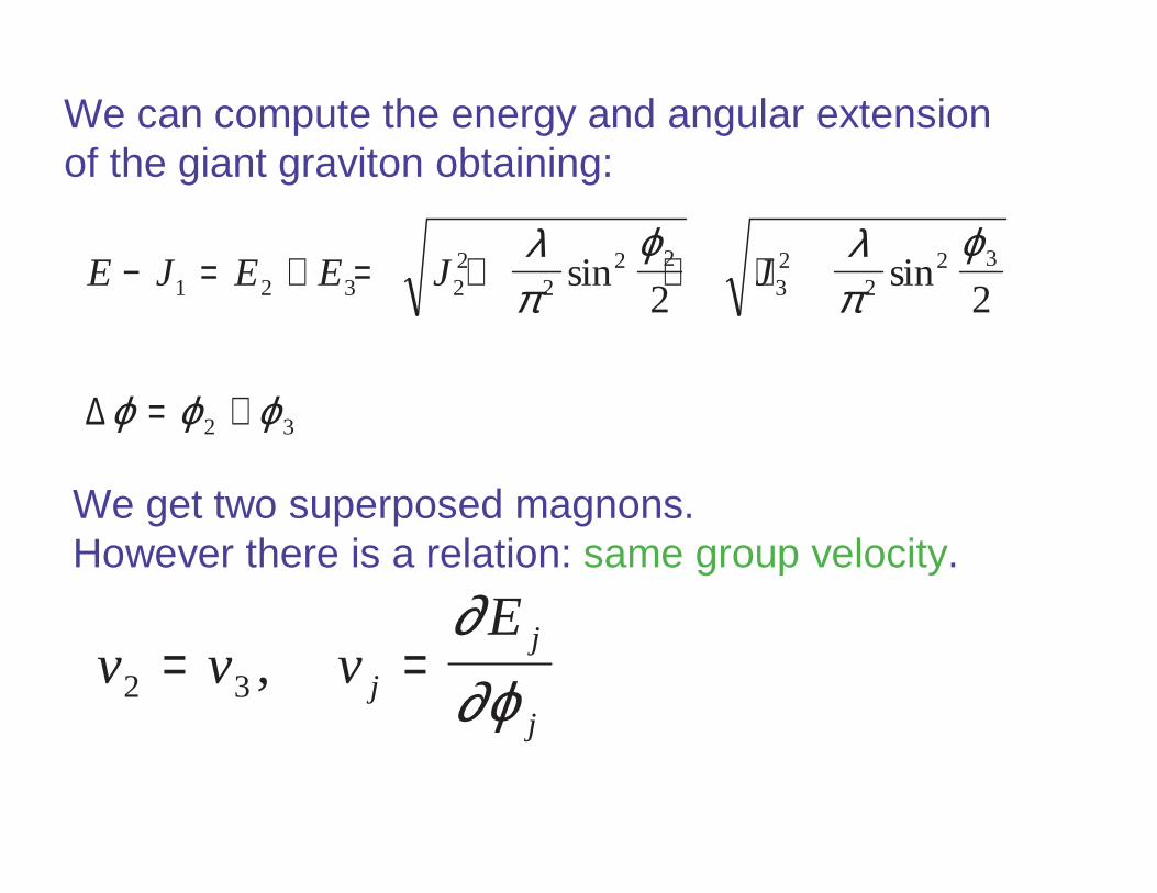
We can compute the energy and angular extensionof the giant graviton obtaining:

E J E E J J− = + = + + +

= +

1 2 3 22

22 2

32

22 3

2 3

2 2

λπ

ϕ λπ

ϕ

ϕ ϕ ϕ

sin sin

∆

We get two superposed magnons. However there is a relation: same group velocity.

v v vE

j

j

j2 3= =,

∂∂ϕ

In the spin chain side we need to use more fieldsto have more angular momenta.We consider therefore operators of the form:

Tr(…XXXXYYXYYZZZYYXXYZZZXXXXXXXXXXXX…)

Where X = 1+ i 2 ; Y= 3 + i 4 , Z= 5 + i 6

The J2 Y’s form a bound state and the J3 Z’s another,both superposed to a “background” of J1 X ’s ( )

The condition of equal velocity appears because in thestring side we use a rigid ansatz which does not allowrelative motion of the two lumps.

J1 → ∞

E J J JJ J

− ≅ + + + < <1 2 32

22 2

32

2 3

2 2 2 21

λπ

ϕ λπ

ϕλsin sin ,

0

0.2

0.4

0.6

0.8

1

–30 –20 –10 10 20 30 40 50

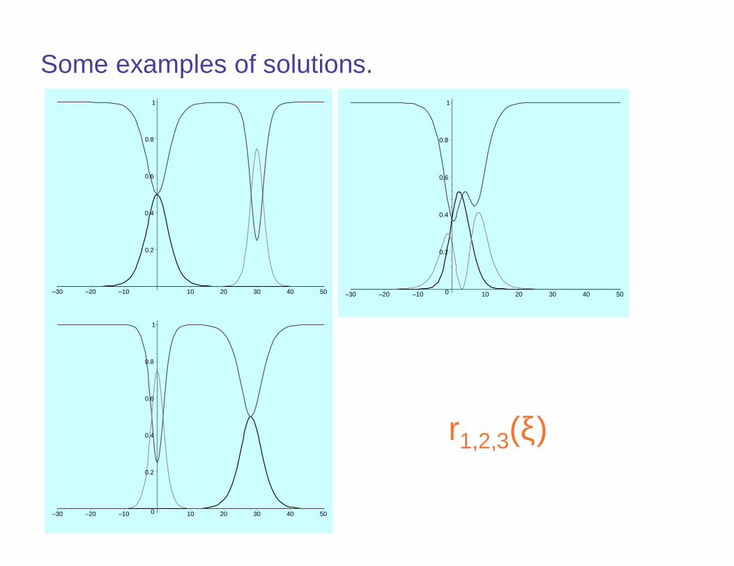
Some examples of solutions.

0.2

0.4

0.6

0.8

1

–30 –20 –10 10 20 30 40 50 0

0.2

0.4

0.6

0.8

1

–30 –20 –10 10 20 30 40 50

r1,2,3(ξ)

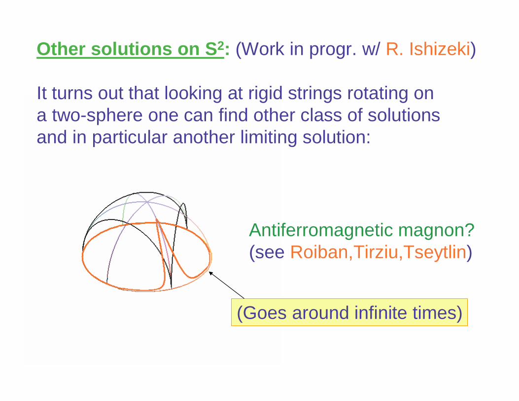
Other solutions on S 2: (Work in progr. w/ R. Ishizeki)

It turns out that looking at rigid strings rotating on a two-sphere one can find other class of solutionsand in particular another limiting solution:

Antiferromagnetic magnon?(see Roiban,Tirziu,Tseytlin)

(Goes around infinite times)

Conclusions:Classical string solutions are a powerful toolto study the duality between string and gaugetheory.

We saw several examples:

folded strings rotating on S5

spiky strings rotating in AdS5 and S5

giant magnons on S2 and S3

giant magnons with three angular momenta

work in progress on other sol. on S2