suction and shear strength relationships of …
TRANSCRIPT

SUCTION AND SHEAR STRENGTH RELATIONSHIPS OF GRANULAR
MATERIALS
Valentine Yato Katte
A thesis submitted to the Faculty of Engineering and Built Environment,
University of the Witwatersrand, in fulfillment of the requirements for the
degree of Doctor of Philosophy.
Johannesburg, 2015

ii
DECLARATION
I, Valentine Yato Katte, declare that this thesis is my own unaided work. It is
being submitted for the degree of Doctor of Philosophy in the University of the
Witwatersrand, Johannesburg. It has not been submitted before for any degree
or examined in any other University.
-------------------------------------------day of ---------------------------------2015.

iii
ABSTRACT
Unsaturated soils are the predominant soil type in moisture deficient areas of the
world. These soils have the characteristic ‘suction’, which is the potential for a
soil to absorb water. With more than one-third of the world located in moisture
deficient zones, understanding the characteristics of these soils is important in
enhancing engineering design and analysis.
Much of the research focus on unsaturated soils is centered on the formulation of
the effective stress equation involving suction and its relevance to strength and
volume change. Suction therefore is a key parameter linked to the behavior of
these soils. It is made up of two components namely matrix and osmotic (solute)
suction of which both are believed to influence soil properties. However, the
exact role of each or both components in influencing the effective stress, strength
and volume change behavior of unsaturated soils has not been fully verified. The
hypothesis postulated is that osmotic or solute suction contributes to the shear
strength of soils.
The focus of this research is experimentally to isolate the effect of osmotic
suction and further evaluate its contribution as well as those of other capillary
forces to the shear strength of granular soils.
The experimental method consisted in altering the suction characteristics of the
pore matrix in granular soils by mixing it with various solutions. This was
achieved by using distilled water, ionic solutions of NaCl and non-ionic solutions
of detergent, and measuring the effects of these solutions on shear strength. In
addition, surface tension measurements were made in a set of capillary tubes
with these solutions and psychrometer tests were made on granular soils mixed
with these solutions. Three sets of triaxial shear strength parameters and
corresponding suction ranges were obtained from the verifications:
Shear strength parameters and matrix suctions measured by the axis
translation technique in the undrained triaxial test.
Shear strength parameters measured in the drained triaxial test.

iv
Shear strength parameters measured in the undrained state on specimens
exposed to different atmospheres in equilibrium with saturated salts
solutions and others exposed to atmospheres in equilibrium with distilled
water, ionic solutions of NaCl and non-ionic solution of detergent.
Results of the experiments revealed that though solute suction may indirectly
influence the shear strength of granular soils, it does not contribute to it in a
direct way. The Bishop equation appropriately describes the strength and
deformable characteristics of unsaturated soils.

v
ACKNOWLEDGEMENTS
I am grateful to Professor G.E Blight who was my supervisor; I appreciate his
guidance, support and advice. Unfortunately he could not live to see the end. I
am grateful to Dr. Irvin Luker who has stepped in to help me go through. I also
acknowledge Dr. Michelle Theron who acted as co supervisor while she was on
staff in the School of Civil Engineering. I appreciate the advice of Professor
Gerhard Heymann of the University of Pretoria. Mr. Norman Alexander assisted
me in the laboratory and Ken Harman machined the triaxial bases. Mr. Bukhosi
M Mathiya did most the drawings.
I appreciate the support and encouragement of the staff, especially those in the
geotechnical group: Luis Torres and Charles MacRobert for support and
encouragement.
I am grateful to the University of Witwatersrand for the some bursaries which
enabled me to go through my research.
To the Minister of Higher Education of Cameroon and the Rector University of
Dschang for granting me study leave.
I am grateful to Mr. Mufor Atanga who suggested South Africa as a possible
study destination to me and enabled me to settle down. Also to the following
families who opened their homes to me in South Africa: Ndoh, Nji, Mynhardt,
Letsaol and the Cheyip’s.
I found spiritual strength from folks within the Navigators, Redeemed Christian
Church, Faith Bible Church and Roosevelt Park Baptist.
I appreciate numerous friends whom I cannot name here, my extended family
and lastly to my wife Nji-Nkah and children Nsiyapnze-Katte, Aloh, and Chakunte
who spent some lonely years without me.

vi
TABLE OF CONTENTS
PAGE
DECLARATION ii
ABSTRACT iii
ACKNOWLEDGEMENT v
CONTENTS vi
LIST OF FIGURES xi
LIST OF TABLES xv
1. INTRODUCTION 1
1.0 Background 1
1.1 Problem statement 2
1.2 Hypothesis 4
1.3 Objective of research 4
1.3.1 General Objective 4
1.3.2 Specific Objectives 5
1.4 Scope 6
1.5 Organisation of thesis 6
2. THE NATURE OF SUCTION IN SOILS 8
2.0 Introduction 8
2.1 The concept of suction 9
2.1.1 Air water interface and surface tension 10
2.1.2 Capillarity 15
2.2.3 Vapour pressure and humidity 18
2.2 Soil suction 21
2.3 Total suction 22
2.4 Matrix suction 23

vii
2.5 Osmotic suction 24
2.6 Soil water potential 24
2.7 Components of soil water potential 25
2.8 Soil water characteristic curve 26
2.9 Methods of expressing suctions 34
3. THE BEHAVIOUR OF UNSATURATED SOILS 36
3.0 Introduction 36
3.1 Stress state in saturated soil 36
3.2 Stress state in unsaturated soil 38
4. SUCTION AND SHEAR STRENGTH MEASUREMENT
IN UNSATURATED SOILS
PART 1 SUCTION MEASUREMENTS 55
4.0 Introduction 55
4.1 Direct matrix suction measurement 55
4.1.1 Suction plate 56
4.1.2 Tensiometers 57
4.1.3 Imperial college tensiometer 58
4.1.4 Osmotic tensiometer 60
4.1.5 Pressure plate 61
4.2 Indirect matrix suction measurement 63
4.2.1 Electrical conductivity sensors 63
4.2.2 Thermal conductivity sensors 65
4.2.3 Time domain reflectometry 67
4.2.4 In-contact Filter paper 69
4.3 Indirect osmotic suction measurement 71
4.3.1 Squeezing technique 71
4.4 Indirect total suction measurement 73

viii
4.4.1 Thermocouple psychrometer 73
4.4.2 Transistor psychrometers (Relative humidity sensors) 76
4.4.3 Chilled –mirror hygrometer 77
4.4.4 Non-contact filter paper 79
4.5 Methods of controlling suction 79
4.5.1 Axis translation technique 80
4.5.2 Osmotic technique 80
4.5.3 Vapour equilibrium technique 81
4.6 Summary 82
PART II SHEAR STRENGTH MEASUREMENT 84
4.7 Introduction 84
4.8 Experimental techniques for testing unsaturated soils 84
4.9 Direct shear box testing 85
4.10 Triaxial Testing 87
4.11 The choice of equipment for research 90
5. EXPERIMENTAL SETUP AND RESULTS
5.0 Introduction 92
5.1 Materials 92
5.1.1 Limestone powder 92
5.1.2 Quartz powder 94
5.1.3 Fine glass beads 94
5.1.4 Particle size distribution 94
5.1.5 Specific gravity determination 95
5.1.6 Sample preparation 95
5.2 Surface tension measurement 96
5.2.1 Experimental theory 96
5.2.2 Surface tension measurement in sealed space 98
5.2.3 Results of surface tension measurement in sealed space 99

ix
5.3 Measurement of total suction 99
5.3.1 Calibration of psychrometers 99
5.3.2 Set up for total suction measurements 101
5.3.3 Results of total measurements 101
5.4 Matrix suction and shear strength measurement 102
5.4.1 Calibration of triaxial cell 102
5.4.2 Consolidated undrained tests 103
5.4.3 Results of Consolidated undrained tests 104
5.5 Consolidated drained Triaxial on saturated specimens 104
5.5.1 Results of Consolidated undrained tests 105
5.6 Consolidated undrained tests on limestone specimens dried in
salts solutions 105
5.6.1 Results of Consolidated undrained tests on limestone
specimens dried in salts solutions 105
6. DISCUSSION OF RESULTS 106
6.0 Introduction 106
6.1 Discussion of surface tension measurements 106
6.2 Discussion of results of total suction measurements 109
6.3 Discussion of results of CU triaxial strength measurements 111
6.4 Discussion of results of CD triaxial strength measurements 118
6.5 Discussion of results of consolidated undrained tests
on limestone specimens dried in salts solutions 121
7. SUMMARY, CONCLUSION AND RECOMMENDATIONS 124
7.0 Summary 124
7.1 Conclusions 124
7.2 Scientific relevance 126
7.3 Recommendations 127

x
8. REFERENCES 128
9. APPENDIX i

xi
LIST OF FIGURES
FIGURE PAGE
1.1 Isotropic stress on soil. 3
2.1 Soil hydrologic system and pressure profiles 9
2.2 Air water interphase 10
2.3 Surface tension phenomenon after Fredlund 1993. 13
2.4 Surface tension on a warped surface. 14
2.5 Behaviour of contact angle for a liquid on a solid. 15
2.6 Forces acting in a capillary tube 16
2.7 Capillary model of partly saturated porous material. 17
2.8 Relationship between total suction and Relative Humidity 23
2.9 Typical soil-water characteristic curves for sand, clay 27
2.10 McQueen and Miller conceptual model for SWCC. 28
2.11 An idealized hysteric soil water characteristic curve. 30
2.12 Hysteresis during consolidation (drying) and swelling 31
2.13 Drying and wetting characteristics found by Croney 32
2.14 A direct comparison of an oedometer consolidation curve
and an atmospheric drying curve using a calibrated
gypsum block to estimate suction. 33
3.1 Effective stress across a soil grain. 38

xii
3.2 (a) Three dimensional stress strain diagram for the swell of
partly saturated soil under constant isotropic load. 44
3.2 (b) Three dimensional stress-strain diagram showing contours
of constant effective stress in partly saturated soils. 45
3.3 (a) Semi quantitative validation of the closed-form equation for
effective stress Group 1 soils: measure and fitted SSCCs for
kaolin, Jossigny silt, Madrid clayey sand and sandy clay 51
3.3 (b) Semi quantitative validation of the closed-form equation for
effective stress Group 1 soils: (b) predicted SWCCs for
these soils. 52
4.1 Suction plate 56
4.2 Soil moisture tensiometer 58
4.3 Imperial college tensiometer ( Rideley et al., 2003) 59
4.4 Osmotic tensiometer (Bocking & Fredlund, 1979) 60
4.5 Pressure plate apparatus 62
4.6 Gypsum block 64
4.7 Thermal conductivity sensor 66
4.8 Pore fluid squeezer 72
4.9 Peltier type psychrometer 74
4.10 WP4 Chilled mirror psychrometer 77
4.11 Calibration characteristic curve for WP4 78
4.12 Shear box apparatus 85
4.13 Triaxial cell 88
5.1 Grain size distribution of granular materials 95
5.2 Experimental set up of glass capillary to measure surface
tension 98
5.3 Calibration curve for psychrometer tip 100
6.1 (a) Effects of ionic solute (NaCl) on the surface tension. 106

xiii
6.1(b) Effects of non-ionic solute (detergent) on the surface tension 107
6.2(a) Water content- total suction curves for Limestone Powder 109
6.2 (b) Water content- total suction curves for Quartz Powder 109
6.2 (c) Water content- total suction curves for Fine Glass Beads 110
6.3 (a) i Maximum deviator stress versus water content for limestone
powder 112
6.3 (a) ii Matrix Suction versus water content for limestone powder 112
6.3 (b) i Maximum deviator stress versus water content for quartz
powder 113
6.3 (b) ii Matrix Suction versus water content for quartz powder 113
6.3 (c) i Maximum deviator stress versus water content for fine glass
beads 114
6.3 (c) ii Matrix Suction versus water content for fine glass beads 114
6.3 (d) sʹ-t' strength diagram showing the limits of measured strength for
limestone powder 115
6.3 (e) s'-t' strength diagram showing the limits of measured strength for
quartz powder 115
6.3 (f) s'-t' strength diagram showing the limits of measured strength
fine glass beads 116
6.3 (g) s'-t' strength diagram showing the limits of measured strength
for the soils mixed with 1 M NaCl at 2 % water content 118
6.4 (a): s´-t´ diagram for Limestone Powder in the CD test 119
6.4 (b): s´-t´ diagram for Quartz Powder in the CD test 119
6.4 (c): s´-t´ diagram for Fine Glass Beads in the CD test 120
6.5 (a) Plots of specimens dried over saturated salts,
re- exposed to solutions of water, 1 M NaCl and
detergent. 121

xiv
6.5 (b) Plots of total suction curves for limestone powder
mixed with water (matrix suction) and limestone
powder mixed with 1M NaCl (matrix + solute suction) 122
6.5 (c) Strength diagram plotted for Limestone powder in
terms of ½(σ1- σ3) and ½(σ1+σ3) –uw where σ3 = 300
kPa and uw = matrix suction for water content when tested. 123

xv
LIST OF TABLES
TABLE PAGE
2.1 Surface tension of contractile skin by (Kaye and Laby, 1973) 12
2.2 Vapour pressures of NaCl solutions by (Lang, 1967) 20
2.3 Vapour pressure of KCl solutions (Campbell & Gardner, 1971) 21
3.1 Soil descriptions and properties used to validate the
Closed- Form Equation for Effective Stress. 51
4.1 Calibrations for estimating suctions by filter paper techniques 71
4.2 Summary of suction measurement methods 83
5.1(a) Chemical properties of limestone powder. 93
5.1(b) Physical properties of the limestone powder 93
5.1 (c) Chemical properties of the silica 94
5.1 (e) Specific gravity of aggregates 95

xvi
APPENDIX
TABLE PAGE
5.1 Grain size distribution of granular material i
5.2(a) Measurement of radii of glass capillaries ii
5.2(b) Surface tension measurements for distilled water and water iii
diluted with ionic solute (NaCl).
5.2(c) Surface tension measurements for distilled water and water iv
diluted with a non-ionic solute (detergent)
5.3 (a) Results of calibration of psychrometer tips v
5.3 (b) Total suction values for Limestone Powder viii
5.3 (c) Total suction values for Quartz Powder ix
5.3 (d) Total suction values for Fine Glass Beads x
5.4 (a-i) Calibration of triaxial cell xi
5.4 (a-ii) Calibration of triaxial machines xv
5.4 (b) Results of triaxial strength parameters and suctions for xvi
Limestone powder
5.4 (c) Results of triaxial strength parameters and suctions for vxiii
Quartz Powder
5.4 (d) Results of triaxial strength parameters and suctions for
Fine Glass Beads xx
5.4 (e) Results of s-t parameters Limestone Powder xxii
5.4 (f) Results of s-t parameters Quartz Powder xxiv

xvii
5.4 (g) Results of s-t parameters Fine Glass Beads xxvi
5.5 (a) Consolidated drained tests for Limestone powder xxviii
5.5 (b) Consolidated drained tests for Quartz powder xxix
5.5 (c) Consolidated drained tests for Fine Glass beads xxx
5.5 (d) The φ´ values of the consolidated drained tests soil. xxxi
5.6 Shear strength parameters of limestone powder in different
saturated solutions then exposed to atmospheres of distilled
water, 1M NaCl and detergent. Initial water content 6%.
total exposure time 6 months. xxxii
APPENDIX
FIGURE PAGE
5.3 Calibration curves for other psychrometers vi-vii

1
CHAPTER ONE
INTRODUCTION
1.0 Background
The mechanics of unsaturated soils is a study that has been given
considerable attention all over the world and more especially in regions
where the average annual evaporation exceeds average annual
precipitation as well as in areas which experience seasonal moisture
deficits. Considering that more than one third of the world falls within the
above described climatic zone (Barbour, 1999), unsaturated soil
mechanics must, of necessity, be basic to geotechnical engineering. The
engineering behavior of soil is intrinsically linked to a soil property termed
suction. Suction simply defined is the potential of soil to absorb water.
The suction concept was first developed in the field of soil science, which
is considerably older than soil mechanics. The concept was originally
developed for the soil-water-plant relationship at the beginning of the
1900’s. It was in the mid twentieth century that soil suction was used to
explain the mechanical properties of unsaturated soils at the Road
Research Laboratory in England (Croney and Coleman, 1948, Croney,
1950). This marked the beginning of unsaturated soil mechanics, even
though some years earlier Terzaghi investigated the effects of
unsaturation in soil devoting a 12 page chapter to capillary forces in soils
(Terzaghi, 1943).
The geo-professional has found it easier dealing with soils that are
saturated than those that are unsaturated because, with the former,
experimentation and formulations of the requisite equations are easier
and more straight-forward than with unsaturated soil. This has therefore
rendered designs in unsaturated soils to be conservative so as to avoid
uncertainties. Still, there have been reported failures of compacted
embankments, excavated and natural slopes and foundations using

2
unsaturated soils, but, with increasing scientific and technological
advancement; there has been an improving degree of certainty in design,
durability and use of this material in construction. Much research is still
required in understanding how the shear strength of unsaturated soil
relates with other soil parameters so as to increase reliability in design
and construction. It is therefore important to evaluate how suction and
shear strength relate so as to improve the knowledge base in this area
resulting in confident interpretation of soil data, better design and
construction with unsaturated soils and so limit potential hazards.
1.1 Problem statement
Much of the research interest in unsaturated soil mechanics revolves
around the formulation of an effective stress equation for these materials
and consideration as to whether, or under what circumstances, the
principle of effective stress applies to unsaturated soils (Blight, 1982, Lu
and Likos, 2006). Terzaghi (1936) originally stated the principle of
effective stress and its relevance to saturated soils. The effective stress
principle states that in an isotropic stress situation a change of volume is
dependent on the difference between total stress and pore pressure as
in figure 1.1 and expressed in equation 1.1. He recognized that the
effective stress, as a stress state variable controls the shearing
resistance and volumetric strains in soils.
∆𝐕
𝐕= 𝐜∆𝛔′ 𝟏. 𝟏
Through this concept, a rational approach at solving soil
mechanics problems for saturated soils (previously very empirical) was
born. The effective stress concept has proved workable in explaining

3
stress and volume changes that occur in saturated soils due to change in
the applied external load.
σ′ = σ − u
Figure 1.1 Isotropic stress applications on soil.
Extending this concept to unsaturated soils has been problematic
because of the presence of pore fluid consisting of two phases; air and
water.
At the inception of unsaturated soil mechanics, suction has been
considered to be the combined effect of matrix and osmotic or solute
suction. These concepts were developed in the disciplines of soil
sciences for soil water and plant relationships, and so far no problems
have been encountered with this concept within this discipline. The
concept was taken over into unsaturated soil mechanics and perhaps it
was assumed that since it worked very well in soil science, then the
same must be true for shear strength and volume change of soils.
Studies so far conducted within this discipline of soil mechanics have not
given a precise and clear presentation how matrix and/or solute suction
affect the shear strength of soils. For example, Sridharan & Venkatappa
Rao, 1973 have asserted that osmotic suction plays a role in determining
the behavior of soils, alluding that current formulations of the effective
σ
u
σ
σ

4
stress equation do not account for osmotic suction. Still continuing in this
thinking Allam & Sridharan, 1987 brought modifications to the effective
stress and stress state variables approach to include osmotic suction
and the contribution of the contractile skin stress. Also, studies carried
out on marine soils indicate that the high salt content contributes to a
high suction which in turn greatly influences the physical and volumetric
changes of soil (Noorany, 1984 ., Barbour and Fredlund, 1989, Fredlund
and Rahardjo, 1993, Feng et al., 2003). Sreedeep and Singh (2006)
have concluded that most studies on suction wrongly approximate total
suction to matrix suction. The basis of this conclusion is the assumption
that the solutes present in the soil are dilute and hence the osmotic
suction is negligible. On the other hand, Blight, (1982) in an attempt to
revive the capillary model, quotes Casagrande’s (1965) attempts to build
a causeway across the Great Salt Lake in Utah. He mentioned that the
clay forming the lake bottom has a shear strength gradient of only 6 kPa
per metre depth. This is despite the fact that the clay contains crystalline
salt and the pore fluid is therefore subject to a solute suction of the order
of 40 000 kPa. Therefore the role of capillary and other intermolecular
forces such as solute suction in the macroscopic stress, strength and
volume change in the behavior of unsaturated soils have been uncertain.
As such it is necessary to investigate the role of osmotic suction as it
influences soil behavior, in particular the shear strength of soil.
1.2 Hypothesis
Osmotic suction significantly contributes to the shear strength of
unsaturated soils.
1.3 Objective of the research
1.3.1 General Objective

5
The aim of this research was to experimentally isolate the effects of
solute and matrix suction and evaluate them separately as well as
examining other capillary forces, relative to matrix suction, while
assessing the shear strength in a set of granular soils.
1.3.2 Specific Objectives
To attain the above general objectives the following specific objectives
where set in place:
1. An array of capillary tubes to be set up to measure the surface
tension of distilled water, water containing an ionic solute (NaCl)
and a non-ionic solute, namely a detergent.
2. Total suction measurements to be made on samples of a number
of different granular materials prepared with distilled water, dilute
NaCl and detergent solutions.
3. Consolidated undrained shear strength measurements to be made
on specimens prepared from the granular materials using the
same solutions and determining their matrix suctions using the
axis translation technique (ATT).
4. Consolidated drained shear strength measurements to be made
on saturated specimens prepared from the granular materials
using the same solutions.
5. Consolidated undrained shear strength measurements to be made
on specimens prepared from the granular materials using the
same solutions after equilibrating in controlled atmospheres of 90-
98 % relative humidity for three months as well as in atmospheres
in equilibrium with pure water, dilute salt and detergent solutions
respectively for three months.

6
6. Pairs of capillary tubes to be set up side by side each within its
own sealed air space, with one dipping into distilled water and the
other into dilute solutions of NaCl and observing the equilibrium
capillary rises.
1.4 Scope
Prior to carrying out the research, an exhaustive literature search was
conducted to examine the work carried out so far on suction and shear
strength relationships of soils. The scope of the work was primarily
experimental with the objectives outlined above. As such, three granular
materials were chosen for this work: limestone powder, quartz powder
and fine glass beads. These were chosen to give aggregates with pH >7
(limestone), < 7 (quartz) and < 7 but also of uniform approximately
spherical particles (glass beads). Suction and shear strength
measurements were taken at various concentrations of pore fluids and at
a range of moisture contents below 10 %.
1.5 Organization of thesis
The thesis has been arranged in the following manner:
Chapter one covers the introduction, problem statement, objectives,
scope and, finally, the organisation of the work.
Chapter two covers the nature of suction in soils.
Chapter three covers the behaviour of unsaturated soils mentioning the
historical developments of the effective stress equation.
Chapter four covers suction and shear strength measurement in
unsaturated soils.
Chapter five describes the experimental set up and results obtained.
Chapter six covers the discussion of results of the experimental set up.

7
Chapter seven covers the summary, conclusions, relevance and
recommendations.

8
CHAPTER TWO
THE NATURE OF SUCTION IN SOILS
2.0 Introduction
Soil is a particulate medium made of numerous discrete particles with a
range of sizes, arranged in a complex geometry which leaves room for
voids. The particle shape, origin, size, and voids influence the soil porous
system. The soil porous system has been characterized as a two phase
or a three phase medium. The two phase medium comprises either
particle solids and water or particle solids and air while the three phase
medium is made up of solid particles, water and air. An unsaturated soil
is defined as one whose voids are filled with water and air, and as such
is often called a three phase system. Fredlund and Morgenstern (1997)
has called the air-water-interface or contractile skin on the liquid menisci,
the fourth phase. It is this fourth phase which renders unsaturated soils
particularly different from saturated soils in terms of engineering
properties. Unsaturated soils are found in arid and semi-arid regions and
where there is a deep groundwater. The climate in these areas is
characterised by an annual evaporation greater than the annual
precipitation. Since the presence of the least air in soils renders them
unsaturated, then most of the soils used as construction materials are in
the unsaturated state and may remain in that condition during the useful
life of the structure. The behaviour of unsaturated soils then becomes
very important in a diverse range of geotechnical and geo-environmental
projects such as earth dams, embankments, waste containment facilities,
slope stability problems and also in agricultural water application to crops
in the unsaturated zone. Therefore phenomena like capillarity, suction
and swelling/shrinkage become important parameters in understanding
the behaviour of unsaturated soils.

9
2.1 The concept of suction
The soil profile acts as a reservoir for water which is stored within the soil
porous system by adhesive, cohesive and capillary forces. Above the
water table three distinct zones have been identified, namely the soil-
water zone, the vadose zone and the capillary fringe. Below the water
table is groundwater. The water table is the boundary at which the pore
water pressure is zero. Above this boundary, the pore pressure is
negative and below it, is positive.
Figure 2.1 Soil hydrologic system and pore pressure profiles
The soil-water zone and the vadose zone contain pores that are partly
filled with air and water and are referred to as the unsaturated zone. The
capillary fringe is just below the vadose zone and is saturated but its
pore pressure is negative or under tension. The unsaturated zone plays
an important role in the biological, physical and chemical processes of
the earth. This zone supports biological life and the intricate slow
weathering processes. Both the saturated and unsaturated zones are
influenced by climatic factors such as precipitation, evaporation and

10
transpiration. The soil in the unsaturated zone is characterised by a
negative pore pressure referred to as suction. There are many other
terms synonymous to suction such as soil moisture deficiency, soil water
pressure deficiency, capillary suction, matrix suction, capillary potential,
capillary water stress, pore water tension, soil water free energy and soil
moisture tension. As you move from the point of zero atmospheric
pressure towards the soil surface, there is increasing desiccation and the
pore water pressure becomes increasingly negative. Curve liquid bridges
can be observed linking soil particles. This curvature is due to the
pressure difference between the air and water phase. The properties of
the air water interface have an important bearing on the mechanical
properties of unsaturated soils. Figure 2.2 below illustrates the air water
interface
Figure 2.2 Air water soil interphase
2.1.1 Air water interface and surface tension
Surface tension is the phenomenon resulting from the physics of the
contractile skin which results from an imbalance of forces acting on the
molecules comprising the liquid phase and air phase. In the case of
Soil
solids
Air
Water

11
water specifically, molecular attraction between water molecules
(cohesion) exerts a stronger pull than the attraction between air and
water molecules (adhesion). This is more evident for molecules located
at the surface where the interaction is greatest, thus creating an
imbalance toward the bulk of the water. For the system to remain in
equilibrium an interfacial tension then develops across the air-water
interface called surface tension. Therefore two distinct entities or
properties are evident: the air-water interface and the bulk water. Davis
and Rideal, (1963) discovered that the properties of the contractile skin
are different from the contiguous water phase. They found that the
contractile skin has reduced density, and increased heat conductivity
while its birefringence data is similar to that of ice. Terzaghi made the
same observation, noting that the properties of the contractile skin are
different from water. The presence of the contractile skin is evident when
an insect such as a water spider walks on top of the contractile skin and
the back swimmer walks underneath it.
Surface tension can be defined thermodynamically as well as
mechanically. Mechanically, surface tension is defined as the force per
unit length required to enlarge the interfacial surface. (Lyklema, 1990,
Adamson and Gast, 1997) Thermodynamically, surface tension has been
defined by Lyklema (2000) as:
𝐓𝐬 = (𝛛𝐅
𝛛𝐀)
𝐕,𝐓,𝐧 𝟐. 𝟏
𝐓𝐬 = (𝛛𝐆
𝛛𝐀)
𝐏,𝐓,𝐧 𝟐. 𝟐

12
where Ts is the surface tension, A is area; F and G are the Helmholtz
and Gibbs energies. The subscript P refers to pressure, T to temperature
and n to the composition of the system. The units of surface tension are
force/length or energy/area, i.e. Nm-1 or Jm-2. The surface tension is
tangential to the contractile skin surface therefore exerting a pull on it. At
20°C the surface tension of water is 72.8 x 10⁻² Nm-1 or Jm-2. Since
surface tension is an intermolecular phenomenon, anything that
influences the intermolecular arrangement will affect surface tension. As
such, surface tension is influenced by temperature and solute
concentration. An increase in temperature causes a decrease in surface
tension. Table 2.1 gives the surface tension values for the contractile
skin of pure water at different temperatures.
Table 2.1 Surface tension of contractile skin of pure water
(Kaye and Laby, 1973)
Temperature T (ºC) Surface tension Ts (N/m)
0
10
15
20
25
30
40
50
60
70
80
100
75.7
74.2
73.5
72.75
72.0
71.2
69.6
67.9
66.2
64.4
62.6
58.8

13
A mathematical relation for surface tension can be established by
imagining a hypothetical curved water surface due to an imbalance of
forces in the bulk of the water. The resulting effect of the imbalance of
forces is a curved air-water interface as shown in the figure 2.3. As
such, a relationship can be drawn between surface tension and radius of
the curved surface.
Figure 2.3 Surface tension phenomenon at the air water interface.
Pressures and surface tension acting on a curved two dimensional
surface (Fredlund and Rahardjo 1993)
The membrane has a radius of curvature Rs and the surface tension is
Ts. The equilibrium of forces in the vertical direction leads to:
𝟐𝑻𝒔𝐬𝐢𝐧𝛂 = 𝟐∆𝐮𝐑𝐬𝐬𝐢𝐧 𝛂 𝟐. 𝟑
2R sin α is the length of the membrane projected into the horizontal
plane.
Rearranging equation 2.3 gives:
∆𝐮 =𝐓𝐬
𝐑𝐬 𝟐. 𝟒
Rs
sss
Rs
α α
Ts Ts
u+∆u

14
Assuming that the shape of the contractile skin is also curved in the
plane perpendicular to that of Figure 2.3 as shown in Figure 2.4.
Equation 2.4 becomes:
∆𝐮 = 𝐓𝐬 (𝟏
𝐑𝟏+
𝟏
𝐑𝟐) 𝟐. 𝟓
If the surface is hemispherical, R1 = R2 = Rs and
∆𝐮 =𝟐𝐓𝐬
𝐑𝐬 𝟐. 𝟔
where ∆u = pressure increase [N/m2]
Rs = radius [m]
Ts = surface tension of water [N/m]
α = subtended at the centre of curvature
Figure 2.4 Surface tension on a warped surface

15
2.1.2 Capillarity
Capillarity is a phenomenon directly related to surface tension. When a
liquid comes to equilibrium with its vapour and in contact with a solid
surface, a contact angle θ is formed and is measured through the liquid
as shown in figure 2.5 below. The contact angle results from equilibrium
between the cohesive forces within the liquid molecules and the
adhesive forces between solid and liquid molecules. For a contact angle
θ = 0°, the surface is completely wet and the solid is perfectly
hydrophilic. A partial wetting of the surface occurs for 0 < θ < 90° and the
solid is partially hydrophilic and when θ ≥ 90° a non-wetting surface
occurs and the solid is hydrophobic. Capillarity will cause water to rise up
in a fine glass capillary because it wets the contact surface due to
surface tension, producing a concave surface at the air-water boundary.
Figure 2.5 Behaviour of contact angle for a liquid on a solid
Figure 2.6 shows water raised to a height hc in a fine capillary of radius r,
then hc, the height of water suspended in the bore is in equilibrium with
the surface tension acting at the bore circumference. Resolving these
forces leads to:

16
Figure 2.6 Forces acting in a capillary tube.
𝟐𝛑𝐫 𝐜𝐨𝐬 𝛉 𝐓𝐬 = 𝐡𝐜𝛄𝐰𝛑𝐫𝟐 𝟐. 𝟕
𝐡𝐜 = 𝟐𝐓𝐬 𝐜𝐨𝐬 𝛉
𝐫𝛄𝐰 𝟐. 𝟖
where: r = radius of fine capillary [m]
Ts = surface tension of water [N/m]
hc = capillary height [m]
This phenomenon is responsible for soil water rising above the
water table in soils. The soil pores act as tortuous capillary tubes with
varying tube diameters. This is what has been termed the capillary
model. A typical graphic presentation of this model for soil is given by
(Marshall, 1959), shown in Figure 2.6. At the top of the capillary bore
where the elastic film exists (contractile skin), the pressure difference
across the film can be expressed by the Young – Laplace equation given
as:

17
∆𝐏 = (𝐮𝐚 − 𝐮𝐰) = 𝟐𝐓𝐬 (𝟏
𝐫) 𝟐. 𝟗
where Ts is the surface tension of the water and r is the radius of the
capillary meniscus.
The Kelvin equation (Aitchison, 1965) represents the pressure
difference as:
∆𝐏 = −𝟑𝟏𝟏𝐥𝐨𝐠 𝟏𝟎𝐇[𝐌𝐏𝐚] 𝟐. 𝟏𝟎
where H is the relative humidity of the pore air above the meniscus.
Substituting the matrix suction (ua-uw) for ∆P in Equation 2.10 enables it
to be expressed as a function of the relative humidity:
(𝐮𝐚 − 𝐮𝐰) = −𝟑𝟏𝟏𝐥𝐨𝐠 𝟏𝟎𝐇 [𝐌𝐏𝐚] 𝟐. 𝟏𝟏
Figure 2.7 Capillary model of partly saturated porous material

18
2.2.3 Vapour pressure and humidity
At the air-water interphace there is the constant exchange of water
molecules between the air and the bulk water. The water molecules that
leave the bulk water form vapour and mix with the air above the air-water
boundary. Some of the vapour condenses and returns to the bulk water.
The kinetic theory offers an explanation of this phenomenon. Some of
the water molecules have sufficient energy to overcome the cohesive
forces and escape the bulk liquid.
Using the analogy of a vessel of air above water, enclosed by a
moveable piston, we can understand better what goes on. If the piston is
withdrawn creating some space above the water, then evaporation
begins and water vapour fills the space. Initially more water vapour
escapes and fills the space than returns into the liquid. Then after some
time equilibrium is attained where the amount of water escaping equals
the amount of water vapour entering. At this equilibrium state, the water
vapour is at its optimum and is called the saturated vapour pressure. As
the piston is withdrawn again further evaporation continues until an
equilibrium state is again attained. Similarly pushing on the piston
causes more water vapour to condense and return to the liquid. If the
temperature of the system is raised, more molecules gain energy and
escape, thus increasing the rate of evaporation and so also the saturated
vapour pressure.
In an open system, similar to the real-life situation where water is
exposed to the atmosphere, evaporation proceeds just as in a closed
system. Dalton’s law of partial pressures becomes applicable. According
to this law a mixture of gases exerts a pressure which is equal to the
sum of the partial pressures of the separate gases.

19
Humidity is a measure of the amount of water vapour contained in
the air. The maximum humidity is obtained at a given temperature when
the partial pressure of water in the air equals the saturated vapour
pressure of water at that temperature. Relative humidity is given as:
𝐑𝐞𝐥𝐚𝐭𝐢𝐯𝐞 𝐡𝐮𝐦𝐢𝐝𝐢𝐭𝐲 =𝐏𝐚𝐫𝐭𝐢𝐚𝐥 𝐩𝐫𝐞𝐬𝐬𝐮𝐫𝐞 𝐨𝐟 𝐰𝐚𝐭𝐞𝐫 𝐯𝐚𝐩𝐨𝐫
𝐒𝐚𝐭𝐮𝐫𝐚𝐭𝐞𝐝 𝐯𝐚𝐩𝐨𝐫 𝐩𝐫𝐞𝐬𝐬𝐮𝐫𝐞 𝐨𝐟 𝐰𝐚𝐭𝐞𝐫 𝐱 𝟏𝟎𝟎% 𝟐. 𝟏𝟐
In the atmospheric sciences condensation is reckoned as either
the formation of dew or frost when the relative humidity attains 100 %.
When air laden with water vapour is cooled sufficiently, condensation
takes place. The temperature at which this condensation begins is the
dew point temperature. This is what takes place at night as the
temperature drops and cools the surrounding air resulting in dew
formation. Applications of this principle have found relevance in some
suction measuring equipment such as relative humidity sensors.
When non-volatile solutes (e.g NaCl) dissolve in pure water, the
vapour pressure of the NaCl-water solution becomes less than that of the
pure water. The addition of the solute has reduced the chemical potential
of the salt solution relative to that of pure water. This reduced chemical
potential is reflected in a reduced kinetic energy therefore less molecular
transfer into the vapour phase occurs. Raoult's law states that for an
ideal solution the partial vapour pressure of a component of the solution
is equal to the mole fraction of that component times its vapour pressure
alone. This law is expressed mathematically by the equation:
𝐕𝐏𝐬𝐨𝐥𝐮𝐭𝐢𝐨𝐧 = 𝐕𝐏𝐩𝐮𝐫𝐞 𝐬𝐨𝐥𝐯𝐞𝐧𝐭 ∗ 𝐌𝐬𝐨𝐥𝐯𝐞𝐧𝐭 𝟐. 𝟏𝟑
where Msolvent = the mole fraction of the solvent

20
VPpure solvent = vapour pressure of pure solvent
VPsolution = vapour pressure of solution
However, for a non-volatile component dissolving in another non-volatile
solution, the partial pressure of any component equals the vapour
pressure of that component multiplied by the mole fraction of the
component.
The vapour pressures of salt solutions (e.g. NaCl and KCl) have
found application in the calibration of suction measuring devices and are
also used to induce suction in soil specimens. Tables 2.2 and 2.3 give
values of (ua-uw) according to equations 2.11 to 2.13 taking into account
different temperatures for NaCl and KCl respectively:
Table 2.2 Vapour pressures of an enclosed air mass over NaCl
solutions by (Lang, 1967)
NaCl
molality
Temperature
0°C 5°C 10°C 15°C 20°C 25°C 30°C 35°C 40°C
Osmotic suction (kPa)
0.05 214 218 222 226 230 234 238 242 245
0.1 423 431 439 477 454 462 470 477 485
0.2 836 852 868 884 900 915 930 946 961
0.3 1247 1272 1297 1321 1344 1368 1391 1415 1437
0.4 1658 1693 1727 1759 1791 1823 1855 1886 1917
0.5 2070 2115 2158 2200 2241 2281 2322 2362 2402
0.7 2901 2967 3030 3091 3151 3210 3270 3328 3385
1.0 4169 4270 4366 4459 4550 4640 4729 4815 4901
1.2 5032 5160 5278 5394 5507 5620 5730 5835 5941
1.5 6359 6529 6684 6837 6986 7134 7276 7411 7548
1.7 7260 7460 7640 7820 8000 8170 8330 8490 8650
2.0 8670 8920 9130 9360 9570 9780 9980 10160 10350

21
Table 2.3 Vapour pressure of an enclosed air mass over KCl (Campbell
and Gardner, 1971)
KCl
molality
Temperature
0°C 10°C 15°C 20°C 25°C 30°C 40°C
Osmotic suction (kPa)
0.0 0.0 0.0 0.0 0.0 0.0 0.0 0.0
0.1 421 436 444 452 459 467 474
0.2 827 859 874 890 905 920 935
0.3 1229 1277 1300 1324 1347 1370 1392
0.4 1628 1693 1724 1757 1788 1819 1849
0.5 2025 2108 2148 2190 2230 2268 2306
0.6
2420 2523 2572 2623 2672 2719 2765
0.7
2814 2938 2996 3057 3116 3171 3226
0.8
3208 3353 3421 3492 3561 3625 3688
0.9 3601 3769 3846 3928 4007 4080 4153
1.0 3993 4185 4272 4366 4455 4538 4620
2.2 Soil Suction
Suction is defined as the free energy state of soil water (Edlefsen and
Anderson, 1943). This is the free energy state of soil water relative to a
pool of pure water at the same temperature and pressure. Depending on
their particle size and distribution, dryer soils may have a higher suction
value than wetter soils. Suction is measured in Pascals = Nm-2 = Nmm-3
= Jm-3 i.e. energy per unit volume. Total suction is made up of two
components: matrix suction, denoted by (𝛙𝐦 ) and osmotic or solute
suction, denoted by (𝛙𝐨 ). The sum of these is called total suction. It is
usually expressed as:

22
𝛙𝐭 = 𝛙𝐦 + 𝛙𝐨 𝟐. 𝟏𝟒
2.3 Total suction
At the soil review panel for the soil mechanics symposium, “Moisture
Equilibria and Moisture changes in Soils’’ (Aitchison, 1964) adopted
some definitions from the International Society of Soil Science which
have been accepted in soil mechanics. Total suction is defined as ”The
negative gauge pressure relative to the external gas pressure on the soil
to which a pool of pure water must be subjected in order to be in
equilibrium through a semi permeable membrane (permeable only to
water molecules) with the soil water’’.
The relationship between total soil suction and the partial pore water
vapour pressure is given by Kelvin’s equation below:
𝛙𝐭 =𝐑𝐓
𝐯𝐰𝐨𝐰𝐯𝐈𝐧 (
𝐩
𝐩𝟎) 𝟐. 𝟏𝟓
where ψt = Total suction [kPa]
R = Universal gas constant [8.314 Nm/Kmol]
T = Absolute temperature [K]
vwo = Specific volume of water [m3/kg]
wv = Molecular mass of water vapour [18.016 kg/kmol]
p = Partial pressure of water vapour in equilibrium with the
soil water [kPa].
po = Partial pressure of the water vapour in equilibrium with
an identical solution at atmospheric pressure [kPa].
The term (p/po) in the Kelvin equation is called the relative
humidity, denoted as RH. The relationship between the relative humidity
and suction is given in the figure 2.8 (below).

23
Total suction ranges from 0 kPa to the region of 1 GPa which
corresponds to a virtually dry state of the soil.
Figure 2.8 Relationship between total suction and relative humidity
2.4 Matrix suction
Matrix suction is defined as ‘‘The negative gauge pressure relative to the
external gas pressure on the soil water to which a solution identical in
composition with the soil water must be subjected in order to be in
equilibrium through a semi-permeable membrane with the soil water’’.
(Aitchison, 1965)
Matrix suction results from capillarity, texture and surface absorptive
forces of the soil matrix. It is expressed as the pressure difference
between the water and air across the air-water interface and is given by
the relation below:
𝛙𝐦 = (𝐮𝐚 − 𝐮𝐰) 𝟐. 𝟏𝟔

24
Referring to the previous chapter for equilibrium at the air water interface
in a thin glass capillary inserted in a vessel containing water, the
pressure difference across the air-water-interface can be expressed as:
(𝐮𝐚 − 𝐮𝐰) =𝟐𝐓𝐬
𝐫 𝟐. 𝟏𝟕
2.5 Osmotic suction
Osmotic suction is defined by Aitchison et al, (1965) as ‘‘The negative
gauge pressure relative to the external gas pressure on the soil to which
a pool of pure water must be subjected in order to be in equilibrium
through a semi-permeable membrane (permeable only to water
molecules) with free pure water’’.
Osmotic suction is also called solute component of free energy of free
water. This arises from the differences in ion concentration of dissolved
salts contained in the soil water.
2.6 Soil water potential
Water movement in soils is controlled by the difference in potentials or
energy in the pores. This is what is referred to as soil water potential.
The state of water in soils is characterized by the amount of water and its
free energy. Three types of energy are involved - potential, kinetic and
chemical. The difference in energy level from one point or state of soil
(wet soil) to another, (dry soil) determines the direction of movement of
water in soils. Soil water movement takes place from a higher potential to
a lower potential. The standard reference is the potential of pure water in
a free state, where the potential is taken as zero. In soils containing
dissolved salts the potential is lower, so water will then flow into it until
equilibrium is achieved. This concept is more used in the soil-water-
plant relationship. In plant physiology positive work is being done as

25
plants take up water against the absorptive forces while negative work is
being carried out when soil absorbs water from plants, causing them to
wilt.
2.7 Components of soil water potential
Water in soil has many forces acting upon it, so its potential energy is
variable within the soil matrix. These forces include:
i. Matrix forces resulting from the interaction of the solid,
liquid and gaseous phases of the soil. The potential for
work to be done by these forces is what is referred to as
the matrix potential, ψm
ii. Osmotic forces resulting from the differences in the
chemical composition of the soil water. The potential for
work to be done by these forces is referred to as the
osmotic or solute potential, ψo
iii. Gravitational forces (and other forces such as (centripetal
forces) are due to their position within those force fields.
The potential for work to be done by the gravitational force
is referred to as gravitational potential energy, Ψp.
The algebraic sum of the energy components of the system is referred to
as total potential and is given by:
𝛙𝐭 = 𝛙𝒑 + 𝛙𝒐 + 𝛙𝒎 𝟐. 𝟏𝟖
where ψt = total potential
Ψp = pressure potential
ψo = osmotic potential
ψm = matrix potential

26
The proportional effect of the components summed in equation 2.18 may
not equal their numerical proportion, e.g if ψo= 2 ψm , it may not be twice
as effective in its action on soil behaviour.
In soil science only the matrix potential and osmotic potential are
considered because only near surface soils within the root zone are of
interest, since the availability of water for plant growth is the major
concern, therefore ψp = 0. Because the flow rate in soils is very low the
kinetic energy is also negligible, therefore the energy state of soil water
is defined only by virtue of its matrix and osmotic components. Assuming
that the dissolved salts are insignificant, the total potential is expressed
in terms of the matrix potential:
𝛙𝐭 = 𝛙𝒎 𝟐. 𝟏𝟗
The matrix potential is given by:
𝚿𝐦 ≡ (𝐮𝐚 − 𝐮𝐰) ≡ 𝐩′′ ≡ 𝐬 𝟐. 𝟐𝟎
Where ≡ means identical, (ua-uw) = pore water suction.
Though soil mechanics and soil science use the same soil-water
terminologies for potential, their interests vary. In soil mechanics the
focus is on strength and volume change, which are controlled by the
effective stress of which some types of potential are a component.
2.8 Soil water characteristic curve (SWCC).
The soil water characteristic curve is a function of the suction in soil and
the water content. It describes the thermodynamic potential of soil
relative to the free water that the soil system tries to absorb. At low water
contents the forces and energy required to move water within the soil
system are high resulting in high suction values. The reverse is the case
with soils having high water contents. Figure 2.9 shows a typical SWCC

27
for sand, silt and clay. The shape and behavior of the SWCC is
influenced by the type of soil, grain size distribution, void ratio, density,
organic matter content, clay content and mineralogy. For example, a
sandy soil has larger pores than a clay soil, so during drying out the
amount of water at a given suction value will be far greater in the clay
soil than in the sandy soil due to the smaller pore diameter which
ensures greater water retention.
Figure 2.9 Typical soil-water characteristic curves for sand and clay
The soil moisture characteristic has been approximated from limited data
as a composite of segments that are simple logarithmic relations by
McQueen and Miller (1974). This is a simple conceptual model which
describes the shape and behavior of the soil water characteristic curve
for sand and is shown in figure 2.10. The line segment from 106 to 104
kPa signifies the region of the tightly adsorbed water regime. The line
segment from 104 to 102 signifies the adsorbed film regime while the line

28
segment from 102 to 0 designates the capillary regime.(Lu and Lukos,
2004) have given an exhaustive description of the various water regimes
in soil, following the McQueen and Miller (1974) model. These are the
tightly adsorbed film segment, adsorbed film segment and the capillary
regime.
Figure 2.10 McQueen and Miller conceptual model for SWCC
In the tightly adsorbed water regime water is held by molecular
bonding mechanisms, primarily hydrogen bonding with the exposed O2-
or OH- on the surfaces of the soil mineral. In the adsorbed water regime
water is held in the form of thin films on the particle surfaces under the
influences of short range solid–liquid interaction mechanisms (e.g.
electrical field polarization, van der Waal attraction and exchangeable
cation hydration). The water content of the first two water regime is
dependent on the soil surface area, surface density and the valency of
the adsorbed exchangeable cations. Once the adsorbed water film
becomes thicker than could be influenced by adsorption effects, then
capillary forces dominate. However, the practical range for suction in
soil does not exceed 3000 kPa and using a log scale for suction distorts

29
the relationship between suction and water content. This is shown when
the McQueen and Miller (1974) data are plotted on both log and natural
scales in figure 2.10. The air entry point is seen to be a function of the
log scale rather than a real changing point on the soil water characteristic
curve. The air entry point is defined by Fredlund and Rahardjo, 1993 as
the matrix suction value that must be exceeded before air recedes into
soil pores.
The degree of saturation (Sr) or gravimetric water content (w) or
volumetric water content (θ) can be used to define the soil water
characteristic curve. The relations between volumetric water content θw,
gravimetric water content, w, and degree of saturation, Sr are given by
the relation below:
In a saturated soil:
𝛉𝐰 =𝐯𝐰
𝐯𝐰 + 𝐯𝐬
𝐰 =𝐌𝐰
𝐌𝐬=
𝐯𝐰𝛒𝐰
𝐆𝐬𝛒𝐰𝐯𝐬=
𝐯𝐰
𝐆𝐬𝐯𝐬=
𝐞
𝐆𝐬 𝐞 = 𝐰𝐆𝐬 𝟐. 𝟐𝟏
𝛉𝐰 =𝐒𝐫𝐞
𝟏 + 𝐞=
𝐰𝐆𝐬
𝟏 + 𝐰𝐆𝐬
In an unsaturated soil:
𝐞 =𝐰𝐆𝐬
𝐒𝐫
𝛉𝐰 =𝐰𝐆𝐬
𝟏 + 𝐰𝐆𝐒𝐒𝐫
⁄=
𝐒𝐫𝐰𝐆𝐬
𝐒𝐫 + 𝐰𝐆𝐬 𝟐. 𝟐𝟐
Where e = void ratio, Gs = specific gravity, ρw = density of water, Ms =
mass of soil solids and Mw = mass of water.

30
Equations 2.21 and 2.22 are just some useful theoretical relationships.
For practical purposes the soil water characteristic curve is always
measured in terms of the gravimetric water content, w.
The relationship between suction and moisture content is not
unique for a particular soil type. This is due to the significant variation in
the water content for a given suction value which is caused by the history
of wetting and drying of the soil. The main drying cycle is obtained by
taking an initially wet soil sample and subjecting it to increasing suction
by drying and measuring the moisture content while the main wetting
cycle is obtained by taking an initially dry soil sample and wetting it and
measuring the moisture content. The main cycles yield continuous
curves which are not identical and separated from each other by wi as
shown in Figure 2.11.
Figure 2.11 An idealised hysteretic soil water characteristic curve

31
From the graph it is evident that the suction value at given moisture
content is greater for the main drying leg than the wetting leg. This
phenomenon is called hysteresis in unsaturated soils. Hysteresis can
significantly alter soil behaviour since two different suction values can be
obtained for the same water content depending on which cycle, either
drainage or wetting, is taking place.
Blight (2013), has attributed hysteresis to non-recoverable energy
consumed by compression of the soil. His explanations come from figure
2.12. This figure shows the consolidation pressure and void ratio plotted
together with their corresponding water contents for saturated Boston
blue clay. Taylor, (1948) had the following as clay parameters:
percentage clay size fraction < 2 μm, PL=20, LL=40 and PI= 20. The
clay was dried by increasing the compression in an oedometer, then re-
wetted by unloading and re-dried again by loading.
Figure 2.12 Hysteresis during consolidation (similar to drying) and
swelling (similar to re-wetting) in saturated clay (Blight, 2007)

32
The area enclosed by the hysteresis loop will have units of w.kN.m/m3
{since the water content is a dimensionless quantity} Area = kN.m/m3 =
1kJ/m3. The hysteresis loop ABC is the energy loss upon loading, to 80
kPa and unloading which is approximately 3.2 kJ/m3. While BCD is the
area enclosed by rewetting, curve BC and the second drying, CD, whose
enclosed area is approximately 0.5 kJ/m3, if closure DB is assumed.
Since the area BCD is not zero, CD and BC do not coincide.
Once a saturated soil is consolidated by drying, it can wet up only
along the rebound curve (see fig 2.11). As a consequence, it is
impossible to have scanning curves. These may be possible only in rigid
porous materials such as ceramics.
Figure 2.13 Drying and wetting characteristics found by Croney,
Coleman and Bridge (1952) for a heavy clay

33
Hysteresis also occurs in natural soils as well as in compacted
soils. In natural soils, hysteresis occurs between the virgin drying line
(VDL) and the subsequent re-wetting limb. Figure 2.13 illustrates
experiments by Croney, Coleman and Bridge (1952) showing
undisturbed clay and clay slurry reaching suctions of up to 100 MPa. As
the clay slurry dries from a water content of 45 % to 5 % and then re-
wets to 17 %, the resultant loop, ABC, demonstrates an energy
consumption of approximately 1300 kJ/m3. In an undisturbed clay
specimen, drying from 21% to 5% and re wetted to 19 %, the EFG loop
shows no energy consumption. This implies that for natural soils that are
over consolidated or over-dried, little or no hysteresis occurs.
Figure 2.14 A direct comparison of an oedometer consolidation curve
and an atmospheric drying curve using a calibrated gypsum block to
estimate suction Blight 2013

34
This is what is experienced by near surface soil deposits in water
deficient climates with repeated wet and dry cycles.
The soil water characteristic curve is simply a pressure
consolidation curve. Since these graphs have axes with similar units,
these two curves can be compared. Figure 2.14 shows a comparison of
these curves for saturated silty clay (Blight, 2013). The loop ABC shows
the SWCC while AXY is the pressure consolidation curve. The silty clay
was consolidated from a water content of 41 % to 24 % at a vertical
stress of 1000 kPa, while atmospheric drying caused the clay to attain a
suction of 1100 kPa at a water content of 30 %. Therefore, the
consolidation of a saturated soil is a more effective approach to dewater
a soil than by surface evaporation. However, consolidation entails more
energy consumption (loop AXY- 40kJ/m3) than surface drying (loop ABC-
20 J/m3)
2.9 Methods of expressing suctions
The terms suction and soil water potential are used
interchangeably by both soil physicists and geotechnical engineers. Soil
water potential is often expressed as the energy per unit quantity of
water. This unit quantity of water could either be mass, volume or weight
so the energy per unit mass of water is Jkg-1, and is also called chemical
potential in kgmol-1. The energy per unit volume is Jm-3 which is
equivalent to pressure, Nm-2. This is a pressure potential. The energy
per unit weight is JN-1 which is equivalent to [m], i.e. a measure of length
or head. In geotechnical engineering, soil pore water potential units of
head [h] or pressure, [ψ], are used in describing stress and deformation
in unsaturated soils. These relationships are summarized in equations
2.23 and 2.24.
Ψ = [Nm-2 = Nm.m-3 = Jm-3] 2.23

35
ρwgh = [kg.m-3 m.s-2.m = kg.ms-2.m-2 = Nm-2 = Jm-3] 2.24
where:
ψ is the pressure [N/m2]
h is the head [m]
g is the gravitational acceleration [m/s2]
ρw is the density of water [kg/m3]

36
CHAPTER THREE
THE BEHAVIOUR OF UNSATURATED SOILS
3.0 Introduction
This chapter presents some historical perspective on the behaviour of
unsaturated soils but with focus on the evolution of shear strength and/or
effective stress equations. The behaviour of unsaturated soils has
received attention from many researchers whose common objective has
been to develop an appropriate expression which adequately models the
shear strength of soil. The choice of appropriate state variables
necessary to describe unsaturated soil behaviour has not been the same
from these researchers. This chapter reviews the historical development
of the equations describing the state of stress in saturated and
unsaturated soils.
3.1 Stress state in saturated soil
According to Lu and Likos (2006) the definition of the concept of effective
stress was formulated by Terzaghi in 1936, though evidence of its
earliest use by Terzaghi dates back to 1926 with the equation:
𝛔′ = 𝛔 − 𝒖𝒘 𝟑. 𝟏
Through this concept a rational approach to solving soil mechanics
problems for saturated soils, which previously was very empirical, was
born. Terzaghi’s concept links deformation and strength uniquely to a
change in the effective stress. It has proven to be practically relevant in
current geotechnical practice where stress, volume, strain and
deformation are analysed for saturated soils. Other researchers like
Rendulic (1936), Bishop and Eldin (1950), Henkel (1960) and Lu and
37
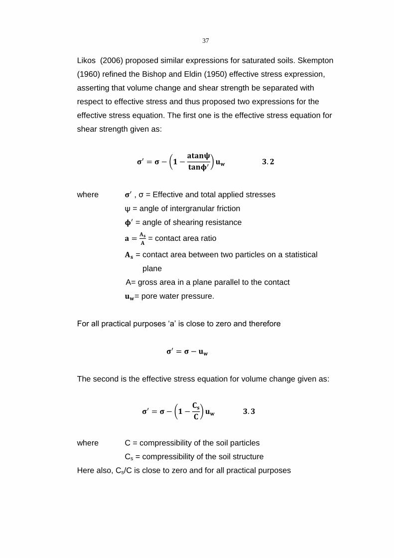
Likos (2006) proposed similar expressions for saturated soils. Skempton
(1960) refined the Bishop and Eldin (1950) effective stress expression,
asserting that volume change and shear strength be separated with
respect to effective stress and thus proposed two expressions for the
effective stress equation. The first one is the effective stress equation for
shear strength given as:
𝛔′ = 𝛔 − (𝟏 −𝐚𝐭𝐚𝐧𝛙
𝐭𝐚𝐧𝛟′) 𝐮𝐰 𝟑. 𝟐
where 𝛔′ , σ = Effective and total applied stresses
ψ = angle of intergranular friction
𝛟′ = angle of shearing resistance
𝐚 =𝐀𝐬
𝐀 = contact area ratio
𝐀𝐬 = contact area between two particles on a statistical
plane
A= gross area in a plane parallel to the contact
𝐮𝐰= pore water pressure.
For all practical purposes ‘a’ is close to zero and therefore
𝛔′ = 𝛔 − 𝐮𝐰
The second is the effective stress equation for volume change given as:
𝛔′ = 𝛔 − (𝟏 −𝐂𝐬
𝐂) 𝐮𝐰 𝟑. 𝟑
where C = compressibility of the soil particles
Cs = compressibility of the soil structure
Here also, Cs/C is close to zero and for all practical purposes
38
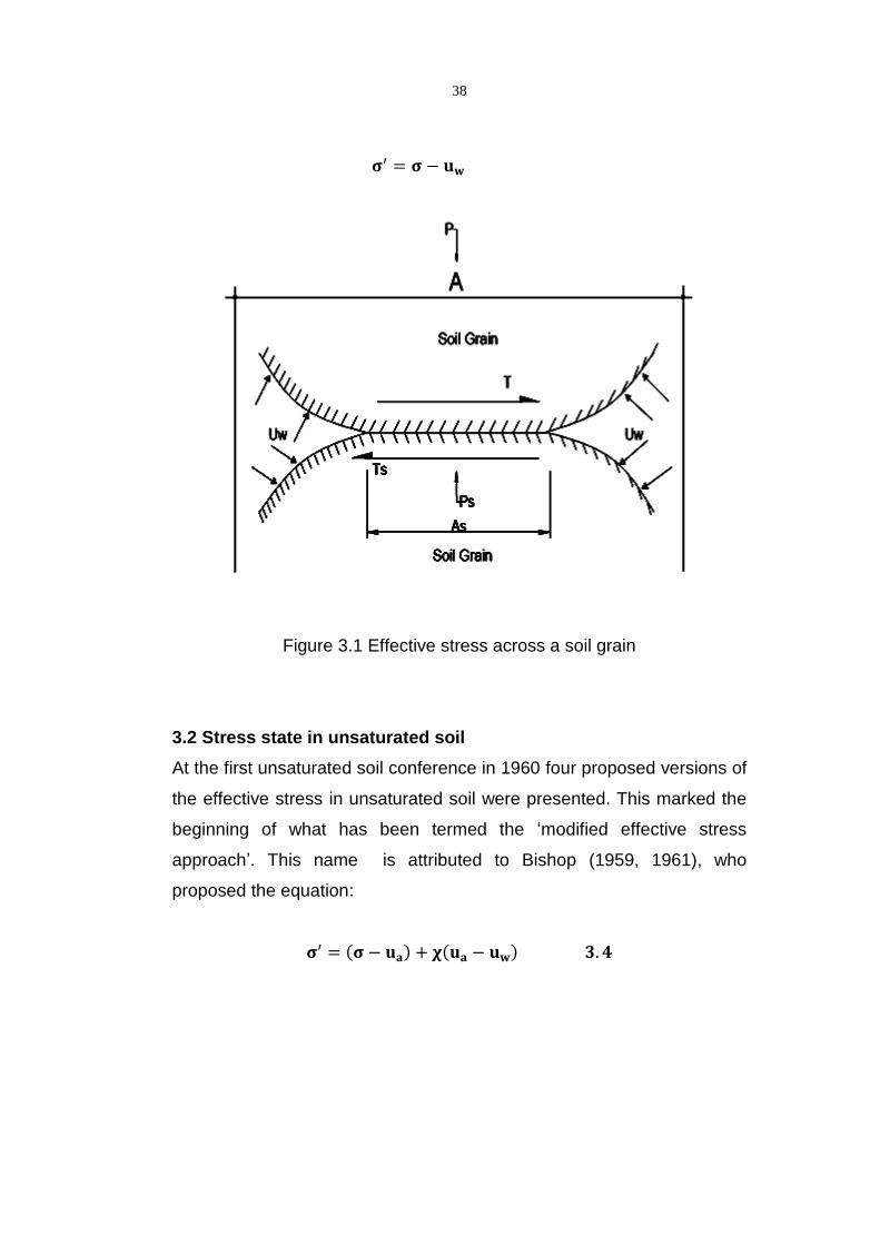
𝛔′ = 𝛔 − 𝐮𝐰
Figure 3.1 Effective stress across a soil grain
3.2 Stress state in unsaturated soil
At the first unsaturated soil conference in 1960 four proposed versions of
the effective stress in unsaturated soil were presented. This marked the
beginning of what has been termed the ‘modified effective stress
approach’. This name is attributed to Bishop (1959, 1961), who
proposed the equation:
𝛔′ = (𝛔 − 𝐮𝐚) + 𝛘(𝐮𝐚 − 𝐮𝐰) 𝟑. 𝟒

39
Where ua and uw are the pore air and pore water pressures respectively
and χ is an empirical factor called the coefficient of effective stress. Its
value varies between 0, for extremely dry soil and 1, for saturated soil.
Aitchison (1961) proposed the equation:
𝛔′ = 𝛔 + 𝛙𝐩′ 𝟑. 𝟓
where p' is the suction or pressure deficiency which is the equivalent of
(ua-uw). The Aitchison equation is a special case of the Bishop equation
when the air pressure is zero (atmospheric).
Jennings (1961) proposed an equation similar to that of Aitchison using a
different symbol, β, in place of either χ or ψ. This equation was dated in
1958 though it was in the 1960s that it was made public.
𝛔′ = 𝛔 + 𝛃𝐩′ 𝟑. 𝟔
The fourth equation, presented at that same conference by Croney
(1958) is given as:
𝛔′ = 𝐩 − 𝛃′𝐮 𝟑. 𝟕
where p is the equivalent of σ and u is the pore water pressure and β is
the bonding factor which is a measure of the effectiveness of the pore
pressure contribution to soil strength. This fourth equation is similar to
the Bishop equation when the air pressure is zero.
The discussions at the 1960 conference on pore pressure and
suction in soils concluded that the equations presented were similar to

40
each other and the Bishop equation was adopted as the equation of
reference for unsaturated soils.
The adoption of the Bishop equation did not close the discussion
on this topic since within a year Lambe (1960) suggested a modified
form of the effective stress equation as given below:
𝛔 = �̿�𝐚𝐦 + 𝐮𝐚𝐚𝐚 + 𝐮𝐰𝐚𝐰 + 𝐑 − 𝐀 𝟑. 𝟖
where �̿� is the mineral to mineral contact stress, am is the fraction of total
cross sectional area that consist of mineral to mineral contact, aa and aw
are the fraction of total cross sectional area occupied by air or water
respectively and R and A are the repulsive, (R), and attractive, (A),
electrical forces. The Lambe equation can be simplified to the following:
�̿�𝐚𝐦 + 𝐑 − 𝐀 ≡ 𝛔′
𝐚𝐰 ≡ 𝐱 𝐚𝐧𝐝 𝐚𝐚 ≡ 𝟏 − 𝐱
From the above relations, it is evident that the Lambe (1960) equation is
equivalent to the Bishop equation.
In 1963, Bishop and Blight published the results of some
experiments to validate the Bishop equation where they demonstrated
that the shear strength and volume change characteristics are
unchanged with effective stress changes when (σ-ua) and (σ-uw) are kept
constant. Three years later Richard (1966) also suggested another
equation for the effective stress, where he included a contribution due to
the effect of osmotic (or solute) suction:
𝛔′ = (𝛔 − 𝐮𝐚) + 𝛘𝐦(𝐮𝐚 − 𝐮𝐰)𝐦 + 𝛘𝐬(𝐮𝐚 − 𝐮𝐰)𝐬 𝟑. 𝟗

41
in which σ' and σ are respectively the effective and total stresses and χ is
Bishop’s effective stress parameter. The subscripts m and s denote
‘‘matrix’’ and ‘‘solute or osmotic suction’’.
Other more recent equations similar to the Bishop’s has been proposed
by other researchers such as Allam & Sridharan (1987); Oberg & Sallfor
(1997) and Sheng et al. (2002).
Allam & Sridharan (1987) proposed the following equation.
𝛔′ = (𝛔 − 𝐮𝐚) + 𝛘(𝐮𝐚 − 𝐮𝐰) − 𝐑′ + 𝛄𝐓 𝟑. 𝟏𝟎
Where R’ is the osmotic suction which tends to disperse soil particle, γ is
the interphase perimeter and T is the surface tension. Since Richard’s
1966 equation which included the effects of solute suction, Sridharan &
Venkatappa Rao (1973) had suggested an osmotic suction addition to
the existing current formulations of the effective stress equation.
Oberg & Sallfors, 1997 proposed the following equation for shear
strength expressed as.
𝛕 = 𝐜′ + {(𝛔 − 𝐮𝐚) + 𝐒𝐫(𝐮𝐚 − 𝐮𝐰)} 𝐭𝐚𝐧 𝛉′ 𝟑. 𝟏𝟏
Sr is equivalent to χ and the equation is similar to the Bishop equation.
Sheng et al. (2002) proposed another equation for the effective stress
expressed as.
𝛔′ = 𝛔 − 𝛅𝐢𝐣(𝐒𝐫)𝐮𝐰, 𝐮𝐚 = 𝟎 𝟑. 𝟏𝟐
When the ua > 0 then the equation is exactly Bishop’s and is given as
𝝈′ = (𝛔 − 𝐮𝐚) − 𝛅𝐢𝐣(𝐒𝐫)(𝐮𝐚 − 𝐮𝐰) 𝟑. 𝟏𝟑

42
Matyas and Radhakrishna (1968) used the concept of constitutive ‘state
surfaces’ to relate void ratio, e, and degree of saturation, Sr, with the net
normal stress σa = (σ-ua) and the matrix suction uc = (ua-uw). The
assumption here was that the principle of effective stress was
inadequate to explain changes in the volumetric behaviour of
unsaturated soils subjected to external loads. They used mixtures of
20% kaolin and 80 % flint powder giving clay of medium plasticity,
compacted to densities of 14 kN/m2. Samples of about 101.2 mm
diameter by 101.2 mm height were made by statically compacting the
kaolin mixture in four layers at the rate of 1.9 mm/min using a
compression machine. The compacted specimen was mounted on a
modified triaxial apparatus having a fine pored ceramic disk, with an air
entry value of 310 kPa. This was the beginning of what has been termed
the ‘two stress method’. They called the equations used to express the
unique relationship between different state parameters ‘state functions’.
In these a physical quantity, for example θ, associated with an element
of a material is uniquely determined by the state of the element and this
gives a unique function as:
𝛉 = 𝐟(𝐉𝟏, 𝐉𝟐, 𝐉𝟑, 𝐒𝟏, … ) 𝟑. 𝟏𝟒
where J1, J2 … are the stress parameters
S1, S2 … are other state parameters
θ is the ‘state point’ function
Furthermore they hypothesized that in the triaxial compression testing of
saturated soils the void ratio and degree of saturation can be expressed
as dependent quantities by the following equations:
𝐞 = 𝐅(𝐩𝐚, 𝐪, 𝐮𝐜, 𝐞𝐨, 𝐒𝐫𝐨) 𝟑. 𝟏𝟓

43
𝐒 = 𝛟(𝐩𝐚, 𝐪, 𝐮𝐜, 𝐞𝐨, 𝐒𝐫𝐨) 𝟑. 𝟏𝟔
Where pa, q and uc are the stress parameters and eo and Sro are the
initial void ratio and degree of saturation respectively.
Blight (1965) represented the stress parameters in a three-
dimensional rectangular coordinate system by generating some
surfaces using unsaturated effective stress variables (σ-ua) and (ua-uw)
with respect to volume change for swelling and collapsing soils. These
were based on experimental measurements and are illustrated in figure
4.2 (a) and (b). Figure 4.2 (a) shows the stress strain diagram for the
swell of partly saturated soil under constant isotropic load. For a
constant (σ-ua) stress situation, a reduction matrix suction (ua-uw), will
cause swelling along line AB. If the grain structure of the soil is stable,
swelling will continue until (ua-uw) = 0 and the soil attains saturation at B.
Swelling will continue further than B along BC’ if (σ) is reduced because
the soil is in a saturated state and ua = 0. If the grain structure is unstable
collapse settlement may occur when suction falls below a critical value of
the applied stress-path DEF. Once the grain structure stabilizes, swelling
resumes along FG, provided that suction continues to decrease and the
soil behaves normally

44
Figure 3.2 (a) Three dimensional stress strain diagram for the swell of
partly saturated soil under constant isotropic load.
Figure 3.2 (b) shows the constant volume swell process of an
unsaturated soil where the suction is reduced by wetting the soil and the
applied stress (σ-ua) is adjusted to prevent swelling or shrinkage from
occurring.

45
Figure 3.2 (b) Three dimensional stress-strain diagram showing contours
of constant effective stress in partly saturated soils.
Aitchison (1969) continued along the same line of reasoning with
the two independent stress variable method and later, Brackley (1971)
carried out some studies on the partial collapse of unsaturated expansive
clays where he independently measured stress variables (σ-ua) and (σ-
uw). He encountered some difficulties in applying the Bishop equation,
describing the volume change behaviour as a function of the
independent stress variables. Fredlund et al (1977) consolidated and
popularised this method. They argued that introducing the χ factor of the
Bishop equation renders it a constitutive relation because χ depends on
the soil characteristics. The possible stress combinations proposed to
describe the stress strain behaviour of unsaturated soils are:
(𝛔 − 𝐮𝐚), (𝐮𝐚 − 𝐮𝐰 )
(𝛔 − 𝐮𝐰), (𝐮𝐚 − 𝐮𝐰)
(𝛔 − 𝐮𝐚), (𝛔 − 𝐮𝐰)

46
In 1978, Fredlund, Morgenstern and Widger proposed three shear
strength equations in terms of pairs of the three independent stress state
variables. These were expressed following the Mohr-Coulomb failure
criterion. The first of these expressions is given as:
𝛕 = 𝐜′ + (𝛔 − 𝐮𝐰)𝐭𝐚𝐧𝛟′ + (𝐮𝐚 − 𝐮𝐰)𝐭𝐚𝐧𝛟′′ 𝟑. 𝟏𝟕
where
c' = effective cohesion parameter
ϕ'= friction angle with respect to changes in (σ-uw) when (ua-uw) is held
constant
ϕ'' = friction angle with respect to changes in (ua-uw) when (σ-uw) is held
constant
Equation 3.17 is advantageous in that it provides for a smooth transition
from the unsaturated to the saturated state. The disadvantage comes
when the pore water changes because the two stress state variables
change.
The second expression is given as:
𝛕 = 𝐜′′ + (𝛔 − 𝐮𝐚)𝐭𝐚𝐧𝛟𝐚 + (𝐮𝐚 − 𝐮𝐰)𝐭𝐚𝐧𝛟𝐛 𝟑. 𝟏𝟖
where
c'' = cohesion intercept when the two stress variables are zero
ϕa= friction angle with respect to changes in (σ-ua) when (ua-uw) is held
constant
ϕb = friction angle with respect to changes in (ua-uw) when (σ-ua) is held
constant.
The advantage of Equation 3.18 is that only one stress variable is
affected when the pore water pressure changes. Regardless of the
combination of stress variables used to describe the shear strength, the

47
value of the shear strength obtained is the same for a given soil provided
that σ, ua and uw remain unchanged.
The third expression for shear strength is given as:
𝛕 = 𝐜′ + (𝛔 − 𝐮𝐚)𝐭𝐚𝐧𝛟′ + (𝐮𝐚 − 𝐮𝐰)𝐭𝐚𝐧𝛟𝐛 𝟑. 𝟏𝟗
Equations 3.17 and 3.19 will give the same value of shear strength
therefore equating them will result in an expression relating the various
angles of friction given as:
𝐭𝐚𝐧𝛟′ = 𝐭𝐚𝐧𝛟𝐛 − 𝐭𝐚𝐧𝛟′′ 𝟑. 𝟐𝟎
Fredlund, Morgenstern and Widger however, favoured Equation 3.19 for
engineering practice.
A third approach to describe the stress state in unsaturated soils
is called the suction stress characteristic curve (Lu and Likos, 2006).
They proposed a form of suction stress that is similar to Terzaghi’s
effective stress for saturated soils (Terzaghi, 1943) and Bishop’s
effective stress for unsaturated soil (Bishop, 1954, 1959). The aim of this
approach is to propose a single stress variable that can model the
mechanical behaviour of earth materials. Forces such as the van der
Waals, double layer forces, surface tension and adhesive forces are said
to interact at the soil solid surface, generating energy which results in
suction stress. Consequently, the suction stress characteristic curve is a
thermodynamic approach. The following reasons were given why this
approach is better than the other two mentioned above:
Suction stress is solely a function of soil suction and therefore
does not require that the effective stress coefficient χ be used
to define effective stress.

48
The suction stress characteristic curve is similar to the soil
water characteristic curve so a single valued function is
uncalled for.
Hysteresis can also be conveniently handled in the suction
stress characteristic curve.
The effective stress equation by the suction stress characteristic curve is
expressed as:
𝛔′ = (𝛔 − 𝐮𝐚) − 𝛔𝐬 𝟑. 𝟐𝟏
where ua is the pore air pressure, σ is the total stress, σ’ is the effective
stress and σs is the suction stress characteristic curve of the soil, where
σs = - (ua-uw)S and S = saturation proportion and (ua-uw) is the matrix
suction.
Using thermodynamic justifications Lu et al., (2010) also
evaluated the tensile stress from the virtual work of increasing the
volume of the soil system with bound residual water. They arrived at an
expression for the suction stress characteristic curve as:
𝛔𝐬 = −(𝐮𝐚 − 𝐮𝐰)𝐒𝐞 𝐟𝐨𝐫 𝐕𝐰 > 𝐕𝐫 𝟑. 𝟐𝟐
where Se = effective saturation, (ua-uw) is the matrix suction, Vw is the
total water volume and Vr is the residual water volume.
From equation 3.21, Lu et al. (2010) proposed an effective stress
equation as an extension of Bishop’s equation and an expansion of
Terzaghi’s equation for all saturations by modifying the contribution to
effective stress as:

49
𝛔′ = (𝛔 − 𝐮𝐚) − [−𝐒𝐞(𝐮𝐚 − 𝐮𝐰)] 𝟑. 𝟐𝟑
= (𝛔 − 𝐮𝐚)—𝐒 − 𝐒𝐫
𝟏 − 𝐒𝐫
(𝐮𝐚 − 𝐮𝐰) = (𝛔 − 𝐮𝐚) − 𝛔𝐬 𝟑. 𝟐𝟒
Where Sr is the residual saturation
The above equation is different from Bishop’s equation with respect to
the degree of saturation but can become Terzaghi’s effective stress
equation, σ' = σ-uw, when it is saturated. An additional extension can be
carried out by applying the relationship between normalised volumetric
water content or the degree of saturation and matrix suction. Using van
Genuchten’s (1980) soil water characteristic curve model, the
normalised degree of saturation is expressed as:
𝐒𝐞 = {𝟏
𝟏 + [𝛂(𝐮𝐚 − 𝐮𝐰)]𝐧}
𝟏−𝟏𝐧⁄
𝟑. 𝟐𝟓
where n and α are empirical fitting parameters of unsaturated soil
properties, n being the pore size distribution parameter and α the
inverse of the air entry pressure of water saturated soil.
A closed-form expression for the suction stress for a full range of
saturation is obtained by substituting equation 3.25 into equation 3.22
and eliminating matrix suction:
𝛔𝐬 =𝐒𝐞
𝛂(𝐒𝐞
𝟏𝟏−𝐧 − 𝟏)
𝟏𝐧
𝟎 ≤ 𝐒𝐞 ≤ 𝟏 𝟑. 𝟐𝟔
A similar closed-form equation for the suction stress for the full range of
matrix suction is obtained by substituting equation 3.25 into equation

50
3.22 and eliminating the degree of saturation giving equation 3.27 and
3.28 for saturated and unsaturated soils respectively:
𝛔𝐬 = −(𝐮𝐚 − 𝐮𝐰) 𝐮𝐚 − 𝐮𝐰 ≤ 𝟎 𝟑. 𝟐𝟕
𝛔𝐬 = −(𝐮𝐚 − 𝐮𝐰)
(𝟏 + 𝛂[𝐮𝐚 − 𝐮𝐰]𝐧)𝐧−𝟏𝐧⁄
𝐮𝐚 − 𝐮𝐰 ≥ 𝟎 𝟑. 𝟐𝟖
Substituting the equations 3.27 and 3.28 into 3.24 yields equation 3.29
(for saturated soils) and 3.30 (for unsaturated soils):
𝛔′ = 𝛔 − 𝐮𝐚 + (𝐮𝐚 − 𝐮𝐰) 𝐮𝐚 − 𝐮𝐰 ≤ 𝟎 𝟑. 𝟐𝟗
𝛔′ = 𝛔 − 𝐮𝐚 +(𝐮𝐚 − 𝐮𝐰)
(𝟏 + 𝛂[𝐮𝐚 − 𝐮𝐰]𝐧)𝐧−𝟏𝐧⁄
𝐮𝐚 − 𝐮𝐰 ≥ 𝟎 𝟑. 𝟑𝟎
Due to the scarcity of data for SWCC and SSCC for same soils Lu et al,
2010 used existing data to validate this model. For soils which have both
the SWCC and SSCC their data was validated by comparing them with
equations 3.25 for SWCC and equations 3.27 for SSCC. Table 3.1 gives
some characteristics of these soils used while figure 3.3 gives semi
quantitative validation of the closed form equation for effective stress.

51
Table 3.1 Soil descriptions and properties used to validate the Closed-
Form Equation for Effective Stress. (Group 1 soils) (Lu et al., 2010).
Name Soil properties ub=1/α n φ' c
Kaolin LL=63 %, PI =33 %
Percent finer than 3
μmm =70, γdmax =1.4
g/cm3
395 1.20 22 24
Jossigny
Silt
LL=37 %, PI =18 %
clay fraction =34,
γdmax =1.7 g/cm3
182 1.54 22 25
Madrid clay LL=32 %, PI =15 %
clay fraction =17,
γdmax =1.91 g/cm3
127 1.63 38 0
Sandy clay No Data
35 1.59 37 0

52
Fig 3.3 Semi quantitative validation of the closed-form equation for
effective stress Group 1 soils: (a) measure and fitted SSCCs for kaolin,
Jossigny silt, Madrid sandy sand and sandy clay and (b) predicted
SWCCs for these soils. (Lu et al., 2010)
From available geotechnical literature it is evident that three
schools of thought have been established with regards to unsaturated
soil behaviour. The modified effective stress approach attributed to
Bishop, the two independent stress approach attributed to Fredlund and
Morgenstern (1977) and the suction stress characteristic curve, Lu and
Likos (2006), Lu et al., (2010).

53
Bishop’s approach has received some criticism especially
concerning the use of χ which some researchers call an elusive
parameter. For example, Coleman (1962) pointed out that χ is related to
soil structure and that no correlation can be found between χ and a
volumetric parameter such as the degree of saturation. However, Khalili
and Khabbaz (1998), Khalili et al. (2004) obtained a unique relationship
upon analysis of 14 different unsaturated soils thus establishing a
relationship between χ and a volumetric parameter and therefore
expressed Bishop’s parameter as:
𝝌 = [(𝒖𝒂 − 𝒖𝒘)
(𝒖𝒂 − 𝒖𝒘)𝒃]
𝜼
𝟑. 𝟑𝟏
where χ is the effective stress coefficient, (ua-uw) is the matrix suction in
the soil samples at failure conditions, (ua-uw)b is the air entry value of the
soil and η = -0.55. This parameter was based on the analysis of data
from 13 soil samples.
Nuth and Laloui, (2008) have also validated Bishop’s equation as
an appropriate constitutive framework for critical state soil mechanics.
While the two independent stress variables approach is popular
and has been able to handle elastoplasticity, critical state soil mechanics
and couple yield limits with some success, ( Alonso et al.,1990, Wheeler
and Sivakumar 1995, Gallipoli et al. 2003), it is plagued with having to
measure separate material properties whose determination in the
laboratory is slow and time consuming. Lu (2008) has also questioned
whether matrix suction is a stress variable and also the physical basis for
the additional shear strength parameter φb. In addition, the two
independent stress states approach cannot be reconciled within the
context of classical soil mechanics for saturated soils. However it can be

54
said that the two independent stress state equations proposed by
Fredlund et al. 1978, are not different from Bishop’s equation. The
relationship between ϕb and χ is given by the relation:
𝐭𝐚𝐧𝛟𝐛 = 𝛘𝐭𝐚𝐧𝛟′ 𝟑. 𝟑𝟐

55
CHAPTER FOUR
SUCTION AND SHEAR STRENGTH MEASUREMENT IN
UNSATURATED SOILS
PART I SUCTION MEASUREMENTS
4.0 Introduction
Suction measurement is very challenging both in the field and in the
laboratory. With recent technological advancements many instruments
have been developed that can be used for this purpose. However, there
are still limitations regarding cost, reliability, range of operation and
suitability for use within either field or laboratory settings. Suction
measurements can be divided into two broad categories, the direct and
indirect methods.
4.1 Direct matrix suction measurement.
In this method, matrix suction is measured by applying capillarity
principles thereby measuring the negative pore water pressure using a
porous material. The porous material has a range of pore sizes which
allows water and solute movement but stops air at the suction desired.
The main aim is to have control of the water pressure separately from
the air pressure. The maximum value of the matrix suction that can be
measured corresponds to the air entry value of the porous material.
Typical porous materials used are sintered glass, sintered bronze and
ceramics. The various techniques available to measure matrix suction
directly include the suction plate, tensiometers, pressure plate and
Imperial college tensiometer or suction probe.

56
4.1.1 Suction plate
This consists of a saturated high air entry ceramic disk attached to a
water reservoir connected to a U tube to which is attached a vacuum
gauge or manometer. Figure 4.1 below shows a sketch of the suction
plate. The suction plate can measure suction between 20–30 kPa.
Higher values of suction between 80-85 kPa can also be attained using
multiple water hanging columns. Beyond this value cavitation occurs
and air enters the system. The equilibrium time of the suction plate is in
hours.
It is operated by placing a soil sample on the saturated ceramic disk.
Water flows from the reservoir into the soil sample, thereby causing a
change in the meniscus which is read off on the scale. The meniscus is
then adjusted to its original position by applying a vacuum. By placing
several soil samples of different moisture contents on the saturated
ceramic plate, various suction values can be obtained and a suction
versus water content curve for the soil sample can be constructed.
Figure 4.1 Suction plate

57
4.1.2 Tensiometers
The tensiometer consists of a water filled tube (reservoir) having a high
air entry ceramic disk at one end and at the opposite end, is attached a
pressure sensing device. The ceramic tip allows the movement of water
between the soil with which it is in contagct and the tube containing the
water (reservoir). The ceramic tip allows the movement of water
including the solutes. However the tensiometer reading is not affected by
the presence of solutes hence it only measures matrix suction and not
osmotic suction. The equilibrium time of the tensiometer is in minutes
and depends on the hydraulic conductivity of the ceramic material, its
thickness and the hydraulic conductivity of the contact soil. Figure 4.2
shows a tensiometer commonly used in the field.
Prior to using the tensiometer, the reservoir is filled with de-aired water
and a vacuum is applied to remove any trapped air bubbles. The
tensiometer works by allowing the flow of water between the water
reservoir and the soil in contact with the tip. When equilibrium is attained
which is usually in a small number of minutes, the stress holding the
water in the reservoir is equal to the stress in the soil. The water stress in
the reservoir is read off on the sensing device attached to the reservoir.
Tensiometers are limited to a suction value of about 100 kPa at sea
level. At higher elevations their range may drop to between 70-80 kPa.
Also, dust particles, dissolved gases and air bubbles, which get trapped
within the instrument, often cause a reduction in the readings since these
serve as possible nucleation sites for cavitation to occur. They can be
used both in the field and in the laboratory.

58
Fig 4.2 Soil Moisture Tensiometer (Soil Moisture Corporation, 1998)
4.1.3 Imperial college tensiometer (suction probe)
These are miniature tensiometers, which were first developed by Ridley
and Burland (1993) at Imperial College. They are high capacity
tensiometers capable of measuring suctions of 1500 kPa. They consist
of a high air entry ceramic disk of 100 kPa attached at the tip of a
transducer. The other end has a diaphragm to which a sensor is
attached. The thin space between the porous disk and the diaphragm is
a water reservoir containing de-aired water. See figure 4.3. When the
probe comes in contact with soil, water flows from the reservoir into the

59
soil due to suction. Consequently the pressure drop in the reservoir is
sensed by the strain guage sensor attached to the diaphragm. Similar
varieties of the suction probe have been developed by Guan and
Fredlund (1997), as well as Tarantino and Mongiovi (2001). Toker et al.
(2004) developed the MIT tensiometer with a face diameter of 38 mm for
use in triaxial soil testing. Subsequently, miniature probes have been
developed by Meilani et al. (2002) and Rahardjo and Leong, (2006) for
direct measurement of matrix suction within the range of 100-500 kPa,
though their range can be extended to 1500 kPa.
Figure 4.3 An Imperial College tensiometer or suction probe (Ridley et
al., 2003)

60
4.1.4 Osmotic Tensiometer
The Osmotic tensiometer was first developed by Zur (1966), Peck and
Rabbidge (1969) and Kassif & Ben Shalom (1971). It makes use of an
aqueous solution of polyethylene glycol PEG (20000) to transmit an
osmotic pressure which is used to measure soil suction. Bocking &
Fredlund (1979) have developed the one shown in Figure 4.4.
Figure 4.4 Osmotic tensiometer (Bocking & Fredlund, 1979)
This instrument is operated by maintaining a high chamber pressure of
between 1380-2070 kPa through the process of osmosis. This is
achieved by immersing the tensiometer in distilled water where a positive
pressure is created in the chamber as water molecules pass through the

61
semi permeable membrane into the chamber but it stops the PEG from
moving out. When the Osmotic tensiometer now comes in contact with
unsaturated soil, the suction causes a net flow of water from the
chamber until equilibrium is attained with the soil. The reduced chamber
pressure is recorded by a pressure transducer which in turn reflects the
suction in the soil. Bocking & Fredlund have found that the pressure
response of the osmotic tensiometer is erratic due to the following
reasons:
The amount of flow into and out of the pressure chamber may be
large enough to significantly affect the soil suction being
measured.
The osmotic pressure may change during the period of flow
because of the change in the osmotic coefficient, molar
concentration or temperature of the chamber fluid (PEG).
The compressibility of the fluid in the chamber and the
expansibility of the chamber may not be constant.
Flow may cause some solution stratification resulting in a change
in the reflection coefficient.
Bocking & Fredlund (1979) also found that the pressure response of the
osmotic tensiometer is a function of the soil properties such as
permeability and compressibility. Hence the osmotic tensiometer has
limited applications in the field and little reference is made of it in
geotechnical literature.
4.1.5 Pressure plate
This consist of a pressure vessel enclosing a saturated high air entry
ceramic disk below which is a small water reservoir mounted on a stand.
The water reservoir is connected to a pressure transducer lying outside
the pressure vessel. Also a drainage pipe is connected to the water

62
reservoir which also vents outside the pressure vessel. A typical
representation of a pressure plate is given figure 4.5.
Figure 4.5 Pressure plate apparatus.
The high air entry ceramic disk separates the air phase from the water
phase and stops air from flowing through but allows water. To carry out
measurements, several soil specimens prepared at the same density
and moisture contents are placed on the ceramic disc. A slight suction is
placed in the chamber such that the soil specimens absorb some water
from the reservoir through the ceramic disc. The air pressure in the
chamber is increased to a given desired value and drainage is permitted.
When the drainage is over, the pressure chamber is opened and one of
the samples is removed for water content determination. This reading is
the first point on the water content suction curve. Subsequent increments
of air pressure are carried out concurrently with their water content

63
determinations of the other specimens to establish other points on the
water content suction curve.
The maximum range of matrix suction measured on the pressure plate is
1500 kPa. The equilibrium time takes several hours to days and is
convenient only for laboratory determination of matrix suction.
4.2 Indirect matrix suction measurement
In this method matrix suction is measured by calibrating the physical
property of the porous material such as the thermal and electrical
conductivity against matrix suction. This is achieved by equilibrating the
porous material with the matrix suction in the soil so that the water
content of the porous material corresponds with the magnitude of matrix
suction of the soil. The methods available to measure matrix suction
indirectly include electrical conductivity sensors, thermal conductivity
sensors, time domain reflectometry (TDR) and in-contact filter paper.
4.2.1 Electrical conductivity sensors
This equipment consists of two concentric electrical electrodes
embedded in a porous block usually made of gypsum. It measures the
electrical resistance of the porous block in contact with the soil whose
suction is to be determined. The electrical resistance of the porous block
decreases with an increase of the water content of the porous block. A
diagram of a typical electrical conductivity sensor (Gypsum block) is
shown in figure 4.6.

64
Figure 4.6 Gypsum block
A calibration curve is established between the electrical resistance of the
block and the moisture content which is indirectly related to suction.
Some of the disadvantages of the porous block include:
The porous block has a long equilibration time of between 2-3
weeks. The equilibration time also varies with matrix suction
ranging from about 6h for a matrix suction of about 50 kPa to
about 2 days for matrix suction of about 1500 kPa.
The sensitivity drops when the matrix suction is greater than 300
kPa.
The salt concentration of the soil affects the electrical resistance
of the block and the readings obtained may not be a true reflection
of the moisture content of the porous block.
The block may be soluble in water leading to an increase in the
salt content of the soil.
The block experiences hysteresis upon wetting and drying.
Some of its advantages include:
It is easy to use and handle.
65
It is useful for suction determination in non-saline soils and can
measure suction within the range of 30-1500 kPa.
It is good for field and laboratory applications.
4.2.2 Thermal conductivity sensors
These were first proposed by Shaw and Baver (1939). Figure 4.7 shows
a design by Fredlund et al. (1994). It consists of an electric heater and a
temperature sensor embedded in a porous ceramic block. The thermal
conductivity of the ceramic porous block is directly proportional to the
thermal conductivity of the ceramic solid and the pore fluid (air and/or
water). The thermal conductivity of water is 25 times that of air, so a
change in thermal conductivity of the block varies directly with changes
in moisture content.
When the porous block is brought in contact with a soil sample, water
flow is established and at equilibrium the suctions in block and soil are
the same. The water content is measured by generating heat at the
centre of the block using the heating element and measuring the
temperature rise. As the moisture content increases more heat will be
dissipated. The undissipated heat will result in a rise in the temperature
of the block which is inversely proportional to moisture content. The rise
in temperature can be calibrated against suction.

66
Fig 4.7 Cross section of thermal conductivity sensor after Fredlund et al.,
1994
Due to the variation in the properties of individual ceramic porous blocks
calibration is required for optimum functioning. This is achieved by using
a pressure plate and applying different matrix suctions to a soil in
direct contact with the sensors. A correlation can now be obtained
between the measured temperature or its related voltage readings and
the matrix suction. The thermal conductivity sensor is used for both
laboratory and field determinations of matrix suction. It is advantageous
in that its readings are not affected by the amount of salt concentration
present in the soil. However the porous ceramic block is influenced by
hysteresis and takes a long time to respond to a change in suction.

67
4.2.3 Time Domain Reflectometry (TDR)
TDR is used for an indirect determination of matrix suction. It was first
used to measure the dielectric properties of materials. The use of TDR
for soil moisture measurements is fairly recent (Topp et al., 1980). Since
then many others have used it, for example Dalton et al. (1984); Kalinski
and Kelly (1993); Benson and Bosscher (1999); Amente et al. (2000) and
Yu and Drneich (2004).
The working principle behind the TDR is based on the travel time of an
electromagnetic wave emitted from a material of electric discontinuity.
The dielectric constant is evaluated from the travel time of the
electromagnetic wave and the length of the waveguide. When the travel
time varies with a change in the characteristics of the material around the
waveguide, its dielectric constant will also vary. The speed of the wave
through the waveguide embedded in the soil can be given with respect of
the dielectric property of the bulk soil as:
𝛆𝐛 = (𝐜
𝐯)
𝟐
= (𝐜 𝐭
𝟐𝐋)
𝟐
𝟒. 𝟏
Where v = velocity of the electromagnetic wave.
c = speed of light in vacuum (3 x 10⁸ m/s).
L = Length of conductor or waveguide length.
t = time of traverse of the electromagnetic pulse to travel between
wave guide length 2L.
εb = Soil bulk dielectric constant.
Water has a very high dielectric constant which ranges between 80-81
compared to say air with a value of 1, ice 4, and soil 3-5. This large
disparity of the dielectric constants makes the method relatively
insensitive to soil composition and texture and thus adequate for liquid

68
soil water measurement. The dielectric property of the soil is inversely
proportional to the waveguide length L and is expressed as:
𝛆𝐛 ∝ (𝟏
𝐋)
𝟐
𝟒. 𝟐
A relationship can then be established between the dielectric property of
bulk soil and that of water content of the soil, whereby its dielectric
property can be determined by the expressions below.
𝛆𝐰
𝛆𝐛= (
𝐋
𝐋𝐰)
𝟐
𝟒. 𝟑
𝛆𝐰 = 𝛆𝐛 (𝐋
𝐋𝐰)
𝟐
𝟒. 𝟒
Where L and Lw is the travel of the wave in bulk soil and wet soil
respectively.
Calibration of the TDR can be carried out using the relationship between
soil bulk dielectric constant, εb and the volumetric water content 𝛉w for
water contents less than 50 %. The relationship is given by Topp et al.
(1980) as:
𝛉𝐰 = −𝟓. 𝟑𝐱𝟏𝟎−𝟐 + 𝟐𝟗𝟐𝐱𝟏𝟎−𝟐𝛆𝐛 − 𝟓. 𝟓𝐱 𝟏𝟎−𝟒𝛆𝐛𝟐 + 𝟒. 𝟑𝐱𝟏𝟎−𝟔𝛆𝐛
𝟑 𝟒. 𝟓
Calibration can also be established by relating the volumetric water
content and suction measured with a pressure plate apparatus, from
which a relation can be drawn with the dielectric constant of the soil.

69
The TDR measures suction in the range of 0-1500 kPa and is excellent
for both laboratory and field measurements. The equilibration time is in
hours. The advantages of the TDR include:
They are excellent for measurement of volumetric water content to
an accuracy of within 1-2 %.
Enable measurements to be carried out quickly.
Calibration requirements are minimal - in many cases soil-specific
calibration is not needed.
Since the TDR has a very narrow response area perpendicular to
the waveguides, the volumetric water contents can be obtained at
very high degrees of vertical resolution and continuous
assessment of soil water measurements is possible through
automation and multiplexing.
The disadvantages include:
It requires sophisticated electronic devices.
There is a high possibility of signal attenuation in saline soils.
It is not recommended for water logged soils or soils having high
organic contents. In such cases the TDR must be calibrated for
these.
4.2.4 In-contact filter paper
This may be classified as the simplest method of measuring soil suction.
It was first used by Hansen (1926) in Denmark, though Gardner (1937);
Fawcett and Collis-George (1967) McQueen and Miller (1968); Al-Khafar
and Hanks (1974) may be credited with having made it popular for
suction measurements. Attempts at using filter paper for measuring
suction in geotechnical engineering are credited to (McQueen (1968); Ho
(1979); Tang (1978); Khan (1981); Gallen (1985); Chandler and
Gutierrez (1986).

70
The filter paper method exploits the water absorptive characteristics of
filter paper. When filter paper is exposed to a soil environment it will
either absorb or desorb moisture until the suction in the soil and filter
paper is equalized. The soil suction is then obtained from determination
of the water content of the filter paper. Two types of filter papers are
commonly used for suction determination: the Whatman No. 42 and the
Schleicher & Schuel No. 589 WH.
The in contact filter paper method is used for the indirect determination
of matrix suction. A filter paper of known weight is brought in direct
contact with the soil specimen and placed in a container which is sealed
with an electric tape and placed in an insulated temperature controlled
box. After equilibration has been attained (after about 7-14 days) the
filter paper is weighed and its moisture content determined. The
accuracy of the method depends on the quality of the filter paper used,
the sensitivity of the weighing balance and the accuracy of the
established calibration curve.
The calibration curve for the filter paper is done by equilibrating the filter
paper in a pressure plate apparatus (or suction plate) at various applied
suction pressures and the moisture content of the papers is determined
separately.
A number of researchers such as Chandler et al. (1992); Leong et al.
(2002) and Power et al. (2008) have carried out the calibrations of
Whatman No. 42 filter paper for both the contact and non-contact filter.
They are shown in table 4.2.

71
Table 4.1 Calibrations for estimating suctions by filter paper technique
Filter paper Reference Calibration equations (s in Pa)
Whatman No 42
Chandler et al., 1992 Leong et al., 2002
Power et al., 2008
Matrix suction log.s =4.84-0.062 w log.s=6.05-2.48 log w Total suction log.s =4.84-0.062 w log.s=5.31-.088 w Matrix suction log.s =2.91-0.023 w log.s=4.95-.067 w Total suction log.s =8.78 -0.22 w log.s=5.31-0.088 w Contact log.s =1.51-0.944 log w log.s=6.71-2.93 log w
w < 47% w > 47% w < 47% w > 47% w ≥ 47% w < 47%
w ≥ 26% w < 26%
37≤ w ≥ 38 w < 26%
4.3 Indirect osmotic suction measurement
Osmotic suction may be present in both saturated and unsaturated soils.
In saturated soils, the osmotic suction remains constant except if there is
an inflow of contaminated water. Osmotic suction increases in
unsaturated soil as it dries due to the increase in the concentration of the
solutes as the water content decreases. An indirect approach to measure
osmotic suction is by using the squeezing technique.
4.3.1 Squeezing technique
The osmotic suction is measured indirectly by determining the electrical
conductivity of an extract of the pore fluid. The pore fluid squeezer

72
technique enables the entire range of osmotic suction to be measured
and is said to give reasonable measurements of suction (Brackley, 1971,
Morgenstern, 1976). This method consists of extracting the pore fluid
from soil samples sandwiched between a compressing piston and a set
of disks at one end, and at the other end another disk, filter paper and a
cylindrical base where a syringe is used to extract the pore fluid. An
example of a pore fluid squeezer is that given by Manheim (1966) shown
in figure 4.8
Figure 4.8 Pore fluid squeezer (Manheim, 1966).
73
By using an osmotic suction versus conductivity curve, the electrical
signals are converted to osmotic suction (Fredlund and Morgenstern,
1977). The results obtained using the squeezing technique by Krahn
and Fredlund (1972) have been reported to be influenced by the
magnitude of the extraction pressure. Experiments carried out on glacial
till and Regina clay required a squeezing pressure of about 34.5 MPa.
The osmotic suctions obtained are shown to agree closely with the total
suction using a psychrometer minus matrix suction measurements from
pressure plate. From their tests, Krahn and Fredlund (1972) attest to the
reliability of the osmotic squeezing technique for osmotic suction
measurement.
4.4 Indirect total suction measurement
Indirect suction measurement techniques require the measurement of
the moisture equilibrium condition of the soil. In this method the total
suction is obtained from the measurements of the vapour phase which is
in equilibrium with the soil sample. Some of the instruments used to
measure total suction indirectly include the thermocouple psychrometers,
relative humidity sensors, chilled mirror hygrometer and non-contact filter
paper. Each of these methods is described below:
4.4.1 Thermocouple Psychrometer
The thermocouple psychrometer is an instrument that is used to
determine soil suction by measuring the relative humidity within the soil.
There are two types of thermocouple psychrometers: the Peltier type
(Spanner, 1951) and the wet loop type (Richards and Ogata, 1958) .
Both types are similar in their mode of functioning which is dependent on
the temperature difference between an evaporating junction and a non-
evaporating junction. They differ from each other in how the evaporating

74
junction is wetted to induce evaporation. A typical Peltier type
thermocouple psychrometer is shown in figure 4.9.
Figure 4.9 Peltier type thermocouple psychrometer
It is made up of a loop of two dissimilar thin wires of about 0.0025 mm
enclosed in a porous ceramic or stainless steel mesh. The two thin wires
comprising the circuit are made of constantan (copper–nickel alloy) and
chromel (chromium–nickel alloy) joined together to form a measuring
junction. The separate ends of the dissimilar wires are connected to
copper connectors, called reference junctions, which then lead to a
voltmeter.
If the measuring junction of the thermocouple, T, is at the same
temperature as the reference junctions there is no voltage generated and

75
the voltmeter reading is zero. If the temperature of the junction, T, is
increased relative to that of the reference junctions then a positive
voltage is induced in the circuit which will be recorded on the voltmeter.
Similarly, decreasing the temperature of junction, T relative to the
reference induces a negative voltage. The Seebeck effect is the
phenomenon of an induced electromotive force in a closed circuit made
up of two dissimilar metals when the two junctions have two different
temperatures.
The Peltier effect involves passing an electric current through the two
dissimilar wires; the measuring junction cools the air below the dew-point
temperature resulting in the condensation of water onto the junction.
When the current dies down, the condensed water evaporates, causing a
further drop of the temperature at the junction of the dissimilar wires.
This drop in temperature of the junction is a function of the rate of
evaporation which is also affected by the amount of atmospheric water
vapor. A Seebeck effect voltage is then induced which is measured by
the voltmeter.
Prior to the use of the psychrometers, these must be calibrated using salt
solutions of known molarity. The psychrometer tips are suspended in the
salt solutions for an hour in a temperature controlled environment and
thereafter the voltage readings are taken. A regression curve between
salt molar solutions and voltage readings is established. These now can
be used to determine suction in soils. The magnitude of induced output
voltage depends on the suction of the soil (relative humidity) and the
temperature. The output voltage is temperature dependent and, as such,
the results can be adjusted to a temperature of 25 °C by using the
formula below after (Brown, 1970; Wiebe et al., 1970).

76
𝐂𝐨𝐫𝐫𝐞𝐜𝐭𝐞𝐝 𝐫𝐞𝐚𝐝𝐢𝐧𝐠 =𝐦𝐞𝐚𝐬𝐮𝐫𝐞𝐝 𝐫𝐞𝐚𝐝𝐢𝐧𝐠
(𝟎.𝟑𝟐𝟓+𝟎.𝟎𝟐𝟕𝐭) 𝟒. 𝟔
Where t = temperature in °C
4.4.2 The transistor psychrometer (Relative Humidity Sensors)
The transistor psychrometer consists of a thermally insulated container
containing two bulbs – the wet and dry transistor probes which act as the
wet and dry thermometers. The sensors measure the relative humidity of
the air space which is in equilibrium with the soil specimen. The wet
transistor holds a standard size of distilled water drop. When an electric
current passes through the circuit, the water on the wet transistor
evaporates resulting in a drop of the temperature of the wet transistor.
The difference in temperature between the wet and dry thermometers
gives the measure of the relative humidity after an equilibrium period of 1
hour, which is related to the soil suction. Its range of suction
measurement is between 100-10,000 kPa. Bulut et al. (2000) have
shown that the transistor psychrometer has a better capability of
measuring total suction at lower moisture levels, compared with other
psychrometric methods.
The transistor psychrometers are calibrated with salt solutions (just like
the thermocouple psychrometers). They are very sensitive to
temperature fluctuations, hysteresis and the size of the water drop. The
voltage reading for zero total suction is obtained when the probes are
exposed for about 4 hours over distilled water and the output adjusted to
an initial zero voltage reading before calibration. Thereafter different
voltage readings at various salt concentrations are recorded, after an
equilibration time of one hour. Thereafter the Kelvin equation 2.15 on
page 22 is used to obtain the total suction.

77
4.4.3 Chilled-mirror hygrometer
This equipment is similar to the thermocouple psychrometer and it
measures total suction between 150 kPa and 60 MPa with an
equilibration time of 5 minutes. Its principle of functioning is based on
equilibrating the liquid phase of water in a soil sample with the vapour
phase of the water in the air space above the soil specimen in a sealed
chamber (Bulut & Leong, 2008). The sealed chamber contains a fan, a
mirror, an optical sensor, an infrared sensor, a thermocouple and a soil
specimen. An example of the device is shown in figure 4.10. The
thermocouple attached to the mirror measures the dew point
temperature, while the fan circulates the air in the sealed chamber and
speeds up vapour equilibrium.
Figure 4.10 Schematic diagram of WP4 chilled mirror psychrometer and
characteristic curve at low suction range

78
An applied Peltier effect cools the mirror until dew is formed and then
heats it to evaporate it. The temperature of the specimen, which is equal
to the temperature of the vapour space, is measured by the infrared
sensor. The temperature of the soil sample and the dew point
temperature are used to determine the relative humidity, from which the
soil suction can be calculated using the Kelvin equation.
A calibration curve is established using standard salt solutions of known
concentrations against their osmotic suctions. Figure 4.11 shows one
established by Bulut et al (2002).
Figure 4.11 Calibration of WP4 chilled mirror psychrometer
Leong et al. (2003) evaluated the accuracy of a chilled mirror dew point
device using compacted soil samples. A thorough calibration of the
instrument using several standard salt solutions was performed.

79
The equilibration time during calibration and total suction measurement
was short, less than 15 min. The total suction measurements on the
compacted samples were compared to the sum of matric and osmotic
suctions of the same soils that were measured independently. The matric
suction of the soils was measured with the null-type axis-translation
apparatus and the osmotic suction of the samples was estimated
from electrical conductivity measurements of the soil water solution
obtained from a pore fluid squeezer device. The test results showed that
total suctions obtained using the chilled mirror dew point device were
always greater than the sum of the matric and osmotic suctions
measured independently.
4.4.4 Non-contact filter paper
The non-contact filter paper method measures the total suction of soil. In
this method the vapour phase separates the filter paper and the soil
which acts as barrier, therefore exchange of solutes is impossible. The
calibration procedure is carried out as given above in 4.3.4. Given,
therefore, an established calibration curve the suction of soil can be
computed from the curve equation using the obtained water content.
The non-contact filter paper method has been used in the field to
measure total suction (Fredlund 1989). It is also suitable for laboratory
conditions and the practical range of suction measurement is between 50
kPa - 30 MPa or higher.
4.5 Methods of controlling suction
These are methods used to control suction in the laboratory. They are
often used in apparatuses such as the triaxial cell, shear box and
odeometer. The three methods available for controlling suction are the
axis translation technique, the osmotic technique and the vapour
equilibrium technique.

80
4.5.1 Axis translation Technique (ATT)
This technique was proposed by Hilf (1956), to control matrix suction in
unsaturated soils. The basic principle of the axis translation technique
(ATT) is to raise the pore air pressure such that positive values of the
pore water pressure are measured. The technique enables the negative
pore water pressure to be measured without cavitation. Since the
negative pore water pressure is also raised, the pressure difference
between the pore air pressure and the pore water pressure is the matrix
suction and its value remains the same. The matrix suction obtained is
limited by the air entry value of the ceramic disks and values of high air
entry ceramic disks of 1500 kPa are readily available in the market.
Usually the water pressure in the water reservoir is kept as close as
possible to zero with no flow permitted. This is what has been called to
as the null axis translation technique.
The main advantage of ATT is that no chemical is used in the process to
control suction therefore the risk of changing the chemistry of the pore
fluid is eliminated. The disadvantages include the possible diffusion of air
through the high air entry discs into the pore water pressure system. The
diffusion of air leads to the formation of air bubbles in the water thereby
influencing measurements. A flushing system is needed to overcome this
(Bishop and Donald 1961; Fredlund 1975; Sivakumar 1993). Also the air
and water phases must be continuous in order to characterize actual
suction within the soil sample.
4.5.2 Osmotic Technique (OT)
This technique has been used to control suction in oedometers (Delage
et al., 1992; Dineen and Burland, 1995; Delage, 2002), the shear box
(Boso et al., 2005) and the triaxial apparatus (Delage et al., 1987; Cui
and Delage, 1996; Ng et al., 2007). The matrix suction is controlled by
allowing the pore water to equilibrate with a salt solution of known
osmotic potential, separated from the soil specimen by a semi permeable
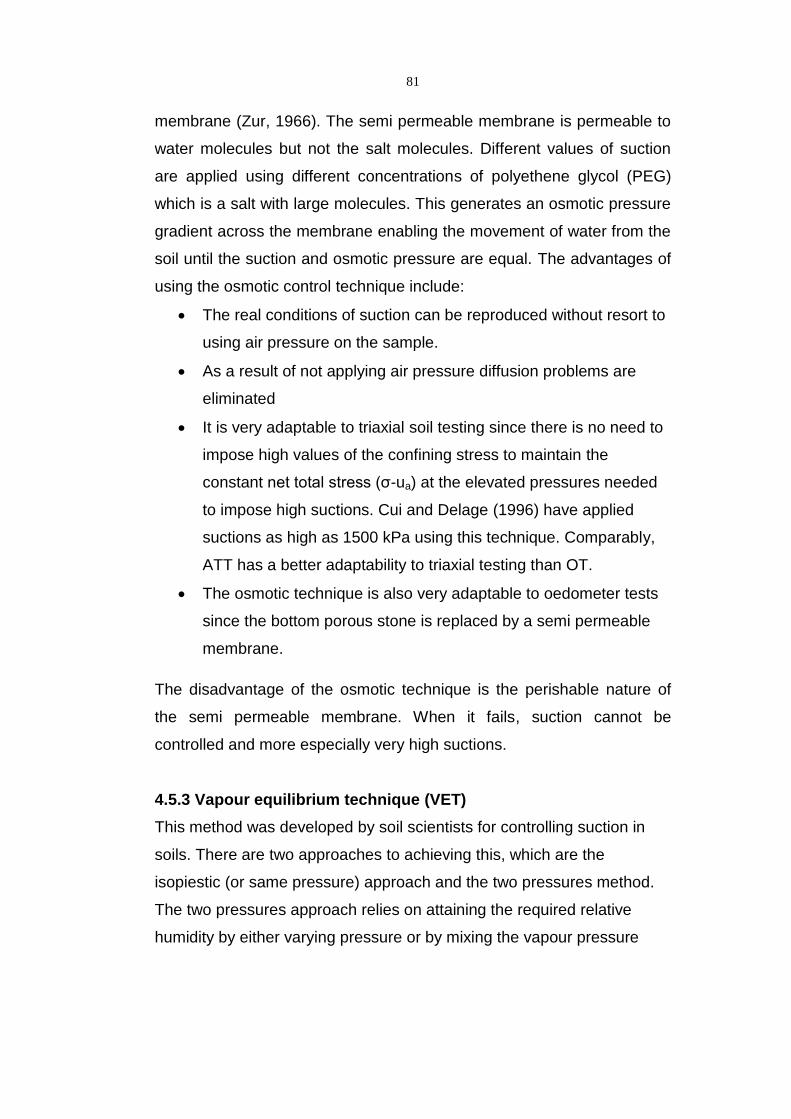
81
membrane (Zur, 1966). The semi permeable membrane is permeable to
water molecules but not the salt molecules. Different values of suction
are applied using different concentrations of polyethene glycol (PEG)
which is a salt with large molecules. This generates an osmotic pressure
gradient across the membrane enabling the movement of water from the
soil until the suction and osmotic pressure are equal. The advantages of
using the osmotic control technique include:
The real conditions of suction can be reproduced without resort to
using air pressure on the sample.
As a result of not applying air pressure diffusion problems are
eliminated
It is very adaptable to triaxial soil testing since there is no need to
impose high values of the confining stress to maintain the
constant net total stress (σ-ua) at the elevated pressures needed
to impose high suctions. Cui and Delage (1996) have applied
suctions as high as 1500 kPa using this technique. Comparably,
ATT has a better adaptability to triaxial testing than OT.
The osmotic technique is also very adaptable to oedometer tests
since the bottom porous stone is replaced by a semi permeable
membrane.
The disadvantage of the osmotic technique is the perishable nature of
the semi permeable membrane. When it fails, suction cannot be
controlled and more especially very high suctions.
4.5.3 Vapour equilibrium technique (VET)
This method was developed by soil scientists for controlling suction in
soils. There are two approaches to achieving this, which are the
isopiestic (or same pressure) approach and the two pressures method.
The two pressures approach relies on attaining the required relative
humidity by either varying pressure or by mixing the vapour pressure

82
saturated gas with dry gas. The isopiestic approach is achieved by
attaining vapour equilibrium for acid or salts in a closed thermodynamic
system. According to Delage et al. (1998), the vapour equilibrium
technique was first used in geotechnical engineering by Esterban and
Saez (1998).
In the vapour equilibrium method the soil specimen is placed in a
thermodynamically sealed system connected to a desiccator containing
aqueous salt solutions of known concentrations. Equilibrium is attained
by the exchange of water with the vapour until the suction in the soil
specimen is equal to the partial vapour pressure.
The vapour equilibrium technique can be attributed all the advantages of
the osmotic technique with the additional advantage that the testing
times can be significantly reduced by using an air circulation technique
employing an air pump ( Blatz and Graham, 2000; Cunningham et al.,
2003; Lloret et al., 2003; Dueck 2004; Oldecop and Alonso, 2004; Alonso
et al., 2005). The main disadvantage is the extremely long time required
for equilibrium to be attained, in some cases 1-2 months.
4.6 Summary
There are so many methods of measuring suction that they cannot be all
mentioned. Just the common ones have been described here, which are
widely used in engineering practice and in research. The table 4.3 gives
a summary of the various methods described, their advantages,
disadvantages, suitability for laboratory or field use and their equilibration
time.

83
Table 4.2 Summary of suction measurement methods
Method/Technique
Suction range (kPa)
Equilibrium time
Laboratory (L) or field application
(F)
Direct suction measurement
Matrix suction
Tensiometer
0-1,500
Minutes
L & F
Suction probe
Indirect suction
measurement
Matrix suction
Electrical conductivity sensor
50-1,500
6-50 hours
L & F
Thermal conductivity sensor
0-1,500
Hours –days
L & F
In – contact filter paper
All
7-14 days
L & F
TDR 0-1500 Hours L & F
Osmotic suction
Squeezing technique
0-1,500 days L
Total suction
Thermocouple Psychrometer
100-10,000
1 hour
L & F
Transistor Psychrometer
100-8000
Hours-days
L
Chilled-mirror hygrometer
150-30,000
10 minutes
L
Non-contact filter paper
All 7-14 days L & F

84
PART II SHEAR STRENGTH MEASUREMENTS
4.7 Introduction
The shear strength of soil is the maximum resistance to shear that the
soil can sustain. When this is exceeded the soil is said to fail. This
usually occurs in the form of slip surfaces. The internal friction angle of
the soil and the cohesion contribute to shear strength of soil. The internal
friction angle is a measure of resistance to interlocking of the soil
particles while cohesion is a measure of the forces which tend to bind the
soil particles together. These two contributions form the Mohr-Coulomb
shear strength equation for saturated soils which has been extended for
unsaturated soils as explained in chapter three.
4.8 Experimental techniques for unsaturated soil testing
The extension of the Mohr-Coulomb shear strength criterion to
unsaturated soils requires that the shear strength parameters c’ and φ’
be determined. For saturated soils these are determined using the
conventional triaxial and direct shear apparatus. However for
unsaturated soils these apparatuses must be slightly modified to make
room for pore air and pore water pressure measurements
simultaneously. Several challenges to the experimental determination of
the shear strength of unsaturated soils have been identified (Blight 2013)
such as:
The need to make a large number of tests to establish the
variation of shear strength with matrix suction.
The long time required to achieve equilibrium in soil samples
before testing.
Specialized equipment for unsaturated soil testing is complicated
and expensive.

85
4.9 The Direct Shear Box Testing
The direct shear apparatus consists of a horizontally split open metal
box. The soil material is placed into the box and one half of the box
moves relative to the other. Vertical forces are applied through a load
frame acting through the top half of the box, while horizontal forces are
applied through a motor driven device. The diagram below gives a
simple illustration of the shear box apparatus.
Fig 5.12 Shear box apparatus
The direct shear apparatus has been modified to be able to test
unsaturated soils. Donald (1956) modified the traditional direct shear box
and reported a series of shear tests on unsaturated fine sands and

86
coarse silts. In his modification the top of the shear box was exposed to
atmospheric pressure while the pore water pressure was controlled.
Escario (1980) also modified the traditional shear box making room for
measurement of both the pore air and water pressures and allowing
suction to be controlled through the axis translation technique. Gan et al.
(1988) have described another modification where the shear box is
enclosed within an air pressure chamber allowing control of the air
pressure in the specimen. The control of pore water pressure was
through a high air entry pressure disk located at the base of the
specimen. The following results can be obtained from a shear box
apparatus:
The peak and residual angles of shearing resistance.
The peak and residual cohesion intercepts.
The volume change response of the soil to shearing (dilatant or
contractant).
The advantages of the direct shear box test are:
The test is relatively simple and quick to perform.
During testing, large shear displacements can be applied enabling
the determination of the soils residual strength.
The time required for specimen consolidation and drainage is
small, because of a small drainage path length equivalent to half
the specimen thickness.
Shearing takes place along a predetermined plane.
Some of the disadvantages and limitations of the direct shear box
include:
Impossible to control drainage, so the soil sample is normally
assumed or tested either as drained or undrained.

87
The stress conditions during test are indeterminate so only an
approximation can be given because they are not uniform. Hence
a stress path cannot be established.
Shear stress failure may develop progressively during testing.
Specimen saturation for example by back pressuring is not
possible therefore specimen must be inundated.
The area of the shearing surface changes continuously, so a
correction for this change of area is needed.
4.10 The triaxial testing
The first triaxial apparatus was developed by Bishop and Henkel (1962)
and up to now only minor improvements have been done on it, such as
the replacement of the mechanical measuring systems with electronic
control systems and data logging facilities. The triaxial equipment can be
used to determine the triaxial strength, stiffness and characteristic stress
(ko) ratio of soils. An illustration of a triaxial cell is given in figure 4.13. In
the testing of unsaturated soils, the triaxial cell has been coupled to
various suction controlling apparatuses. The most common uses the
axis translation technique. The use of the osmotic control technique in
triaxial testing has been reported by Cui & Delage (1996) while the
vapour control technique has also been reported (Blatz & Graham 2000,
Chavez et al., 2009). Some triaxial testing devices have also been
developed using psychrometers (Tang et al., 2002 and Thom et al.,
2008) as well as high capacity tensiometers (Colmenares & Ridley,
2002; Meilani et al., 2002 and Jotisankasa et al., 2007).

88
Figure 4.13 Triaxial cell
In present practice the following types of triaxial tests are carried out.
Unconsolidated undrained tests denoted (UU) with or without pore
pressure measurement.
Isotropically consolidated undrained compression (CIU) test with
or without pore pressure measurement.
Isotropically consolidated drained compression (CID) test.

89
In compression triaxial testing the soil specimen is acted upon by three
stresses. The vertical axial stress is the major principal stress σ1, while
the intermediate stress σ2 and the minor principal stress σ3 are equal and
corresponds to the cell pressure. (Brenner et al. 1997)
The following types of results can be obtained from triaxial soil testing
(Brenner et al. 1997):
The strength envelope with peak angle of sharing resistance and
cohesion intercept (either in total or effective terms)
The pore pressure response to shearing (in undrained tests)
The volume change response to shearing (in drained tests on
saturated soils and drained and undrained in unsaturated soils)
Tangent and secant moduli ( or corresponding unloading and
reloading moduli) for the soil
Consolidation characteristics
Air and water permeability under different confining pressures and
flow gradients
The advantages of the triaxial shear include (Brenner et al. 1997):
Control of drainage is possible as well as the measurement of
pore pressures.
Stress conditions in the soil sample remain more or less constant
and are more uniform than in direct shear test. They are
controllable during test and their magnitude is known with fair
accuracy.
Volume changes during sharing can be determined accurately
The disadvantages and limitations of the triaxial tests include (Brenner et
al. 1997):
The influence of the intermediate principal stress σ2 cannot be
evaluated. In certain practical problems which approximate the

90
conditions of plain strain σ2 may be higher than σ3. This will
influence c’ and φ’.
The principal stress direction remains fixed, and conditions where
the principal stresses change continuously cannot be simulated
easily.
Influence of the end restraints (end caps) causes non uniform
stresses, pore pressures and strains in the test specimens and
barrel shape deformation, all of which must be considered and
corrected for where possible.
4.11 Choice of equipment for research
The resistance of a soil specimen to deformation at the macro scale is
closely linked with the soil particle arrangement and interactions at the
micro scale. The choice of equipment was to specifically replicate what
seems to take place at the micro level which in turn affects the macro
scale.
At the micro scale the intermolecular forces were modelled using
capillary tubes with varying pore fluid concentration. The suction
response of the varying pore fluid was obtained using a psychrometer.
The motivation for using these two tests above is because of their
simplicity and availability. Meanwhile at the macro scale the interest was
measuring the shear strength. The triaxial equipment was preferable for
this because both the saturated and unsaturated soil tests could be
performed on them with very minimal adaptations. The axis translation
technique (ATT) was easily applied on the specimens. The consolidated
drained test is best carried out on triaxial equipment. The shear box was
also available but it needed an enclosure so that air pressure could be
applied. Using the shear box for unsaturated soil testing would require
more challenging techniques in measuring drainage as well as pore

91
pressures. Different combinations of axial stress and cell pressure are
possible only on the triaxial test.

92
CHAPTER FIVE
EXPERIMENTAL SETUP AND RESULTS
5.0 Introduction
This chapter describes the materials used, the sample preparation, the
equipment calibration and the experimental procedure adopted to study
the relationship between suction and shear strength in unsaturated soils.
5.1 Materials
In keeping with the objective of investigating the role of suction in the
shear strength of soil, aggregates were selected which will not react (or
will have as little reaction as possible) with the mixing fluids. Clayey soils
were avoided because of the possible reaction of the clay minerals with
ionic and non-ionic solutes. The materials ranged from slightly inert
(limestone powder) having a pH > 7 to inert (quartz powder) pH < 7 and
to completely inert (fine glass beads) pH < 7.
5.1.1 Limestone powder
The limestone powder was sourced from a specific calcrete deposit in
the Northern Province where it has been obtained for more than 50
years. The cream colored limestone went through a well-controlled
milling process. The chemical and physical properties of the limestone
powder are given in tables 5.1(a) and 5.1(b).

93
Table 5.1(a) Chemical properties of limestone powder.
Chemical composition Percentage (%)
SiO2
Al2O3
Fe2O3
CaO
MgO
Na2O3
K2O
CO2
8
1
0.4
49
1
0.1
< 0.1
40
Total 99.5
Table 5.1(b) Physical properties of the limestone powder.
Property
Putty Limestone
Natural colour
Reflectance (Photovolt)
Colour in oil
Oil absorption
Moisture
pH
SG
Bulk density
Light cream
< 70
Dark cream
13-15 %
1-2%
9
2.67
0.95-1.2

94
5.1.2 Quartz powder
The quartz powder was sourced from a supplier in Johannesburg and
the chemical properties of the silica are given in table 5.1 (c).
Table 5.1(c) Chemical properties of the silica
Chemical composition Percentage (%)
SiO2
Al2O3
Fe2O3
TiO2
ZnO2
MgO
CO2
98.01
0.3
0.2
0
0
0.01
0.12
Total 98.64
5.1.3 Fine glass beads
The fine glass beads were available in the laboratory. These were
preferable since they were smooth and rounded and were within the
range of fine sand fraction.
5.1.4 Particle size distribution of Aggregates
The particle size distributions of the aggregates were determined in
accordance with ASTM 422 on dry aggregates. The particle size
distributions obtained for the three aggregate materials are given on
table 5.1 found in appendix pp. i and their grain size distribution curves
are shown in figure 5.1. All these materials consist predominantly of
particles the size of fine sand.

95
Figure 5.1 Grain size distribution of granular material.
5.1.5 Specific Gravity Determination
The specific gravity of the aggregates was determined in accordance
with ASTM 854-00. The results of the specific gravity of the aggregates
are given in table 5.1 (e)
Table 5.1 (e) Specific gravity of aggregates
Aggregates Specific gravity
Limestone powder
Quartz powder
Fine glass beads
2.67
2.65
2.48
5.1.6 Sample preparation
The mixing fluids used in preparing the sample were distilled water,
molar solutions of NaCl and detergent solutions. The molar solutions
were obtained by dissolving molar quantities of NaCl in one litre of
distilled water. 1 kg each of the aggregates were weighed into a mixing

96
bowl. The corresponding mixing fluid at moisture contents of 2, 4, 6, 8
and 10 % by mass was added to it and these were thoroughly mixed and
kept in plastic containers which were sealed and kept for 48 hours for
moisture equilibration. These were carried out for distilled water, various
molar solutions of NaCl and detergent solutions. The specimens were
statically compacted in a cylindrical mould of diameter 38 mm and 76
mm high in three layers. For each layer 50 g of moist aggregate mix was
used. The void ratios of the specimens were estimated from the relation.
𝐞 = 𝐆𝐬(𝟏 + 𝐰)𝛄𝐰
𝐌𝐚𝐬𝐬𝐯𝐨𝐥𝐮𝐦𝐞⁄
− 𝟏 𝟓. 𝟏
The limestone powder was compacted to a bulk density of 1741 kg/m3
giving void ratios ranging from 0.56 at 2 % moisture content to 0.69 at 10
% moisture content respectively. Quartz powder was compacted similarly
to the same bulk density giving void ratios of 0.55-0.67 at 2% to 10 %
moisture contents respectively. The fine glass beads were compacted to
a density of 1671 kg/m3 by weighing 48 g compacted in three layers,
giving void ratios of 0.51 at 2 % moisture content to 0.63 at 10 %
moisture content.
5.2 Surface tension measurements
5.2.1 Experimental Theory
The phenomenon of capillarity which is responsible for water rising
above the water table has been exploited in order to measure surface
tension. This is what has been termed the capillary model. A typical
presentation of this model for soil is given by Marshall (1959), shown in
Figure 2.6, in section 2.1.2. Equation 2.8 can be re- arranged to give
equation 5.2 for the surface tension force in terms of the water rise in a
capillary tube

97
𝐓𝐬 =𝛄𝐰𝐡𝐜𝐫
𝟐 𝟓. 𝟐
The surface tension was estimated from the height of water in the
capillary assuming that the contact angle was zero since a clean glass
was used.
The capillary tubes were clamped vertically and concentrated sulphuric
acid was used to clean the glass by injecting the acid slowly through the
capillary. Water was used to rinse the capillaries several times and then
they were dried in an oven at 105 ⁰C for ten minutes. After cooling to
room temperature, the radius of the capillaries was measured by
injecting a known weight of water from a syringe. The radius of the
capillary was estimated from the density volume relationship given below
𝐯 = 𝐦
𝛒= 𝛑𝐫𝟐𝐡 𝟓. 𝟑
𝐫 = (𝐦
𝛒𝛑𝐡)
𝟏𝟐⁄
𝟓. 𝟒
The temperature of the water used was recorded as well the laboratory
temperature and the relative humidity of the air in the laboratory. The
results of measurement of the radius of the capillaries are given in Table
5.2 (a) in appendix pp. ii.
The surface tension was measured by clamping two clean capillary tubes
vertically over two beakers containing various molar concentrations of
pure sodium chloride (0, 0.25M, 0.5M, 0.75M and 1M) and a non-ionic
detergent at concentrations 0, 0.5 g/l, 1g/l and 2g/l. These capillaries
were open to the 20˚C temperature-controlled laboratory. The relative
humidity inside the laboratory was 61%. The capillary rise hc in each

98
case was measured and three separate experimental repetitions were
carried out. The surface tension was calculated from the relation in Eq.
5.1
Figure 5.2 Experimental set up of glass capillaries to measure surface
tension
5.2.2 Surface tension measurements in sealed space
A second experimental set up was made with the capillary tubes, side
by side as before, but each within its own sealed air space, with one tube
dipping into a beaker of pure water and the other into a 1M NaCl
solution. These were left for four weeks to see if, with time, the capillary

99
rises would change as the humidity of the air above the menisci
equilibrated with the liquid forming each meniscus.
The capillary tubes were left untouched and the two containers of
liquid swapped, so that the capillary tube filled with pure water was now
dipping into a beaker of salt solution and vice versa. Both remained
within the same sealed air space for four weeks.
5.2.3 Results of Surface tension measurements in sealed space
The results of the surface tension measurements for distilled water,
water diluted with ionic solute (NaCl) and water diluted with a non-ionic
solute (detergent) for the first set of experiments are given in the Table
5.2 (b) and (c) in appendix pp. iii-iv. While for the second set of
experiments no change in the meniscus levels were observed in either
case.
5.3 Measurement of Total Suction
5.3.1 Calibration of psychrometers
The psychrometers were calibrated to obtain the regression equation
unique for each of the psychrometer tips. The calibration procedure was
as follows:
1. Holes were drilled in the lid of a container.
2. The psychrometers’ tips were passed through these holes to an
appreciable length and the holes were properly sealed with a
silicon sealant and allowed to dry.
3. A salt solution of known molarity was placed in the container and
the lid attached such that the psychrometers’ tips was suspended
over the solution.
4. The container was placed in a water bath and the temperature
maintained at 25° C for a period of 1 hour

100
5. The leads of the psychrometer were connected to an HR 33 T
voltmeter and three measurements of the total suction value in
microvolts were carried out.
6. The process was carried out for different salt solutions.
7. The psychrometer tips were washed and dried after each set of
measurements before re-use.
8. The results of the calibrations of the psychrometers are given in
table 5.3 (a) in appendix pp. v.
9. The calibration curve for one of the psychrometer tips is shown
below while the rest is in the appendix pp. vi-vii.
Figure 5.3 Calibration curve for psychrometer tip
y = 0,2339x - 0,0619 R2 = 0,9995
0
0.5
1
1.5
2
2.5
3
3.5
4
4.5
5
0 10 20 30
To
tal su
cti
on
(M
Pa)
Microvolts μV
Thermocouple PSY SN 48225

101
5.3.2. Set up for total suction measurements
1. Specimens of the granular soil materials were mixed with distilled
water, NaCl solution or 2g/l detergent solution at gravitational
moisture contents of 2, 4, 6, 8, and 10 % and cured in sealed
plastic containers for moisture equilibration for a period of 48
hours.
2. The prepared samples were then sealed in test tubes with the
calibrated psychrometer tips suspended in the sealed air space
above the soil materials for one hour before the suction
measurements were taken.
3. The sealed test tubes were inserted in a water bath having a
controlled temperature of 25 °C. The leads of the psychrometers
were connected to a WESCOR HR-33T DEW POINT
MICROVOLTMETER.
4. The results obtained were corrected for each of the
psychrometers tips using the calibration regression curves
established.
5.3.3 Results of total suction measurements
The results of thermocouple psychrometer measurements carried out on
limestone powder, quartz powder and glass beads at a range of solution
contents of (1-10%) using distilled water (control), 0.25 M, 0.50 M, 0.75
M, 1 M NaCl solutions and 2g/l detergent are given in Tables 5.3 (b), (c)
and (d) in appendix pp. viii-x. ‘Real Mc’ stands for the target moisture
content expected while ‘Lab Mc’ stands for the moisture content obtained
after the aggregates have been mixed, cured for 48 hours and the
suction determined using a psychrometer.

102
5.4 Matrix suction and Shear Strength Measurement
5.4.1 Calibration of triaxial cell
1. Brass pedestals 38 mm diameter with a recess 4mm deep and 35
mm diameter were made.
2. 500 kPa high air entry ceramic disks were sealed into the recess
using an epoxy adhesive.
3. These were placed in beakers containing warm distilled water and
vacuumed at 70 kPa until air bubbles were no longer coming out
of the disks.
4. These were then mounted on the triaxial cell base and the cell
was filled with de-aired water.
5. The triaxial cell was pressurized incrementally and the cell
expansion and the pore water pressure were recorded.
6. A regression curve was established between applied pressure
and cell expansion also another regression curve between applied
pressure pore water pressures for each of the triaxial cells.
7. Readings of the calibration are presented in Table 5.4 (a)-(i) in
appendix pp. xi-xv.
8. Pressure was maintained at 700 kPa and the ceramic disks were
repeatedly purged by opening and closing the valves quickly to
release trapped air.
9. Limestone powder was mixed with water at 2 % moisture content
and kept to equilibrate for 48 hours in sealed plastic bags.
10. Triaxial specimens of diameter 38 mm and 76 mm long were
prepared by compacting the material in three 50 g layers in a
triaxial mould.
11. The specimens were quickly extruded and mounted on the triaxial
base, enclosed with a rubber membrane and sealed from the
environment at the triaxial base and the top cap with O-rings.

103
12. The triaxial jacket was replaced and filled with de-aired water and
its pressure raised to 500 kPa. A 200 kPa air pressure was
simultaneously applied through the top cap.
13. After 8-10 hours of consolidation the shearing was carried out at
the rate of 2 %/ hour over 10 hours.
14. The effective confining pressure used was 500-200 = 300 kPa so
the value of cell expansion at this pressure was used in the
calculations of the deviator stresses.
15. The pore water pressure at each instant during testing was
recorded uw.
16. The suction at failure is obtained by (ua-uw)
17. A summary of sample calibration for 2% limestone powder is
shown on table 5.4 (a)-ii on appendix pp. xv.
5.4.2 Consolidated undrained tests
These were carried out on limestone powder, glass beads and quartz
powder. The aggregates were separately mixed with distilled water
(control), 0.25 M, 0.50 M, 0.75 M and 1M NaCl solution and 2g/l
detergent solutions and sealed in separate plastic bags for 48 hours to
allow moisture equilibration. Specimens of 38 mm diameter and 76 mm
height were made by statically compacting 150 g (fine glass beads 144
g) of aggregates in a cylindrical mould. The specimens were sealed
using a rubber membrane onto de-aired ceramic disks having an air
entry value of 500 kPa. The axis translation technique (Hilf, 1956) was
used with an air pressure, ua, of 200 kPa, applied through the top cap
and a confining pressure, σ3, of 500 kPa. Consolidation was achieved
within 8-10 hours. Thereafter each specimen was sheared at constant
water content at a rate of 2 % /hour, giving a time to failure of 10 hours.
The pore water pressures were measured via a system filled with pure
water, and represent matrix suction only. This is so since no semi

104
permeable membrane separated the water from the salt in the pore
water, and salt ions were free to migrate into the water filling the pore
pressure measuring system. In support of this statement Mitchell (1962)
reported that no measurable osmotic pressure was detected across a 4
inch thick porous stone with 0.5 N NaCl solution and water placed on
opposite sides for a period of 24 hours. The body of each triaxial
specimen would have been subject to the full solute suction as well as
the measured matrix suction.
5.4.3 Results of consolidated undrained triaxial strength
measurements
The results of the consolidated undrained triaxial test carried out on the
three granular soils are given in tables 5.4 (b), (c) and (d), in appendix
pp. xvi-xxi.
5.5 Consolidated drained triaxial tests on saturated specimens
Specimens of 38 mm diameter and 76 mm height were made by
compacting 150.0 g of mixed aggregates (limestone powder or quartz
powder) in a cylindrical mould in three layers. These were sealed to the
pedestal of a triaxial cell using a rubber membrane. The glass beads
were sealed in a similar manner, with measured weights of the glass
beads compacted (144 g) in a split mould mounted on the pedestal. A
positive back pressure using the appropriate distilled water, 1M NaCl
solution, or 2g/l detergent solution, was applied through the triaxial base
till saturation was achieved in the sample. Once a B-value of about 0.9
was achieved in the back-pressured specimen, it was sheared with the
back pressure maintained constant and at a rate of 2 % per hour.
These tests were intended to find if solute suction has any effect on
shear strength when the matrix suction is completely absent.

105
5.5.1 Results of consolidated drained triaxial strength
measurements.
The results of the consolidated drained tests performed on the soil
samples mixed with distilled water, 1 M NaCl solution and 2g/l detergent
with the back pressure being either water, 1 M NaCl solution or 2g/l
detergent are given in tables 5.5 (a), (b) and (c) in appendix pp. xxviii-
xxx.
5.6 Consolidated undrained triaxial strength measurements on
limestone specimens dried in salt solutions.
Specimens from limestone powder were moulded at 6% water content
from mixes made with distilled water, 1M NaCl and 2g/l detergent
solutions. These were made by compacting 150 g of moist limestone
powder in a cylindrical mould to dimensions of 38 mm diameter and 76
mm long. These specimens were oven dried to a constant mass, at a
temperature of 50°C for 24 hours. Thereafter, they were dried over
saturated solutions of ZnSO4 (90% RH), Na2SO4 (93% RH), and K2SO4
(98% RH) in desiccators for three months. After this, some of the
specimens were tested in consolidated undrained compression using a
confining stress, σ3= 300 kPa, at a constant rate of 2% per hour. Those
specimens which were not sheared were re-exposed to atmospheres
over distilled water, 1M NaCl and 2g/l detergent solutions for another
three months, making a total of six months. After the expiration period of
six months, the specimens were sheared as in the case above.
5.6.1 Results of consolidated undrained triaxial strength
measurements on specimens dried in salt solutions.
The results of consolidated undrained triaxial strength measurements on
limestone powder are summarized in table 5.6 in appendix pp. xxxii.

106
CHAPTER SIX
DISCUSSIONS OF RESULTS
6.0 Introduction
The various tests results obtained are discussed in this chapter.
6.1 Discussion of surface tension measurements
The results of the surface tension measurements for distilled water,
water diluted with ionic solute (NaCl) and water diluted with a non-ionic
solute (detergent) are given in the Table 5.2 (b) and (c) on appendix
pages (iii) and (iv). The corresponding graphs are given in figures 6.1(a)
and 6.2(b) respectively.
Figure 6.1(a) Effects of concentration of ionic solute (NaCl) on the
surface tension.
Increasing NaCl concentration causes a very slight increase (10 %) in
surface tension while detergent at a concentration of 2g/L causes a 50 %
reduction of surface tension. This observation implies that dissolving
sodium chloride in the water had virtually no effect on the capillary rise
and hence on surface tension and so capillarity is a purely physical
0
20
40
60
80
100
0 0.5 1 1.5 2 2.5
Surf
ace
tensi
on (
N/m
)
Molar concentration (mol/L)
Exp 1 Exp 2 Exp 3

107
surface effect and does not depend on the internal stresses in a solution
that gives rise to solute or osmotic suction.
Figure 6.1(b) Effects of concentration of non-ionic solute (detergent) on
the surface tension
This appears to contradict the assumptions of Raoult’s law, which
implies that, as more solute is dissolved in a fluid a lower relative
humidity is obtained which consequently translates to a higher value of
suction which, if the Kelvin equation is taken at face value, ought to
translate to a higher meniscus rise in a thin capillary.
From Raoult’s law, the relative humidity, H, in equilibrium with an
aqueous solution is given by:
H = nw
nw+ns 𝟔. 𝟏
where nw = number of moles of solvent and
ns = number of moles of solute.
Also according to Kelvin’s equation (Aitchison, 1965), the corresponding
total suction is given by the equation:
0
20
40
60
80
0 0.5 1 1.5 2 2.5Surf
ace
tensi
on (
N/m
)
Mass per litre of detergent (g/L)
Exp 1 Exp 2 Exp 3

108
𝐡𝛄𝐰 =𝐑𝛉
𝐦𝐰𝐥𝐨𝐠𝐞[H] 𝟔. 𝟐
where h = height to which a solution in equilibrium with a relative
humidity, H, would rise in a capillary of given radius,
R = universal gas constant,
θ = absolute temperature and
mw = molecular mass of water.
Substituting for H in 6.2 gives:
(𝒖𝒂 − 𝒖𝒘)𝐭𝐨𝐭𝐚𝐥 =𝐑𝛉
𝐦𝐰𝐥𝐨𝐠𝐞 [
nw
nw+ns] 𝟔. 𝟑
The results obtained when NaCl was dissolved in water were
different and show that capillary rise depends on a static balance
between the upward surface tension forces and the downward weight of
the column of liquid. It is representative of matrix suction and is not
affected by the solute suction of the liquid column. In other words,
equation 6.2 does not seem to be correct.
The capillary rises did not change in either case when near-
identical capillary tubes were set up side by side as described above.
Further, upon swapping the two containers of liquid, again the rises were
unchanged. Both of these observations show that the height of capillary
rise in a capillary tube is governed by the value of the surface tension
and the radius of the capillary, as shown by equation 6.2, and not by the
relative humidity above the meniscus. In other words, capillary rise is
governed by the intermolecular forces of cohesion and adhesion and not
by the relative humidity above the meniscus.

109
6.2 Discussion of results of total suction measurements
The results of thermocouple psychrometer measurements carried out on
limestone powder, quartz powder and glass beads at a range of solution
contents of (1-10%) using distilled water (control), 0.25 M, 0.50 M, 0.75
M, 1 M NaCl solutions and 2g/l detergent are given in Tables 5.3 (b), (c)
and (d) in appendix pp. viii-x. The resultant graphs for these are given in
Figures 6.2 (a), (b), and (c).
Figure 6.2 (a) Water content- total suction curves for Limestone Powder
Figure 6.2 (b) Water content- total suction curves for Quartz Powder
0
1
2
3
4
5
6
7
8
0 2 4 6 8 10
Suct
ion
(M
Pa)
Gravimetric moisture content (% by weight)
0.25 M NaCl
0.50 M NaCl
0.75M NaCl
Control
2g/l Det
1 M NaCl
0
1
2
3
4
5
6
7
8
0 2 4 6 8 10
Su
ctio
n (
MP
a)
Gravimetric moisture content (% by weight)
0.25M NaCl
0.50 M NaCl
0.75 M NaCl
Control
2g/l Det
1M NaCl

110
Figure 6.2 (c) Water content- total suction curves for Fine Glass Beads
In these graphs, the suctions were calculated from equation 6.3. It is
evident that the curves for water and 2g/l detergent are almost
coincident, i.e. 50 % reductions in surface tension have little effect on
matrix suction.
When distilled water is the pore fluid the suction values obtained must be
entirely matrix suction and the addition of detergent makes very little
difference. For 1M NaCl, the suction must be entirely solute suction at
higher water contents, with a significant matrix suction component at low
water contents. At high water contents where matrix suction is low, the
measured solute suction is very close to that calculated from Equation
6.3 i.e. 4.812 MPa. The calculation is as follows.
For every mole of sodium chloride added to water we have two moles of
solute. Therefore the solute suction contribution of 1 M NaCl solution at
25 °C is given below:
NaCl(s) → Na+(aq) + Cl-
0
1
2
3
4
5
6
7
8
0 2 4 6 8 10
Suct
ion
(M
Pa)
Gravimetric moisture content (% by weight)
0.25 M NaCl
0.50 M NaCl
0.75 M NaCl
Control
2g/l Det
1 M NaCl

111
Number of moles of water in 1 litre nwater = 55.56 moles
Sodium chloride dissociates into Na+ (aq) + Cl- ( two moles of solute)
Number of moles of solute nsolute = 2*1 =2
𝐇 =𝐧𝐰𝐚𝐭𝐞𝐫
𝐧𝐰𝐚𝐭𝐞𝐫 + 𝐧𝐬𝐨𝐥𝐮𝐭𝐞= 𝟎. 𝟗𝟔𝟓
∆𝐏 = −𝟑𝟏𝟏𝟎𝟎𝟎 𝐥𝐨𝐠 𝟏𝟎(𝟎. 𝟗𝟔𝟓)
= −𝟒𝟖𝟏𝟐 𝐤𝐏𝐚
Using the Kelvin equation, the effect of dissolving 1M NaCl has been
calculated. The effect of the solute corresponds to a lower vapour
pressure above the air-water interface and hence a lower relative
humidity. This corresponds to an increase in (ua-uw) from solute or
osmotic suction. However the readings we often obtain from the
psychrometer are often attributed to total suction which therefore creates
a problem with the fundamental assumption already established from the
Kelvin equation. Total suction should therefore be higher taking that total
suction is matrix suction plus solute suction.
6.3 Discussion of results of consolidated undrained triaxial strength
measurements
The results of the consolidated undrained triaxial test carried out on the
three granular soils are given in tables 5.4 (b), (c) and (d) on appendix
pp. xvi-xxi. The maximum peak deviator stresses versus water content at
failure and the suctions obtained at failure versus water content are
given in figures 6.3 (a), (b) and (c) for limestone powder, quartz powder
and fine glass beads respectively.

112
Figure 6.3 (a) i Maximum peak deviator stress versus water content for
consolidated undrained triaxial tests on limestone powder.
Figure 6.3 (a) ii Matrix Suction at failure versus water content for consolidated undrained triaxial tests on limestone powder.
0
200
400
600
800
1000
1200
1400
1600
1800
2000
0 2 4 6 8 10 12
Max
imu
m d
evi
ato
r st
ress
(kP
a)
Water content (%)
Control
0.25M NaCl
0.50 M NaCl
0.75 M NaCl
1 M NaCl
2g/l Det
0
50
100
150
200
250
300
0 2 4 6 8 10 12
Suct
ion
(kP
a)
Water content (%)
Control
0.25 M NaCl
0.50 M NaCl
0.75 M NaCl
1 M NaCl
2g/l Det

113
Figure 6.3 (b) i Maximum peak deviator stress versus water content for
consolidated undrained triaxial tests on quartz powder.
Figure 6.3 (b) ii Matrix Suction at failure versus water content for
consolidated undrained triaxial tests on quartz powder.
0
200
400
600
800
1000
1200
1400
1600
0 2 4 6 8 10 12
Ma
xim
um
dev
iato
r s
tress
(k
Pa
)
Water content (%)
Control
0.25 M NaCl
0.50 M NaCl
0.75 M NaCl
1 M NaCl
2g/l Det
0
5
10
15
20
25
30
35
0 2 4 6 8 10 12
Suct
ion
(kP
a)
Water content (%)
Control
0.25 M NaCl
0.50 M NaCl
0.75 M NaCl
1 M NaCl
2g/l Det

114
Figure 6.3 (c) i Maximum peak deviator stress versus water content for
consolidated undrained triaxial tests on fine glass beads.
Figure 6.3 (c) ii Matrix Suction at failure versus water content for
consolidated undrained triaxial tests on fine glass beads.
From figure 6.3 it can be seen that the suction at failure in the soils was
little affected by the presence of sodium chloride or detergent. The
0
100
200
300
400
500
600
700
800
900
0 5 10 15Max
imu
m d
evia
tor
stre
ss (
kPa)
Water content (%)
Control
0.25 M NaCl
0.50 M NaCl
0.75 M NaCl
1 M NaCl
2g/l Det
0
2
4
6
8
10
12
14
16
18
0 2 4 6 8 10 12
Suct
ion
(kP
a)
Water content (%)
Control
0.25 M NaCl
0.50 M NaCl
0.75 M NaCl
1 M NaCl
2g/l Det

115
suction values obtained in the fine glass bead specimens were very low
and so had very little effect on shear strength. The maximum peak
deviator stresses show similar characteristics, with the effect of
increasing water content being relatively little affected by the presence of
dissolved substances.
Figures 6.3 (d), (e) and (f) show s'- tʹ strength diagrams for t’=
½(σ1- σ3), and upper and lower limits of sʹ i.e ½(σ1+σ3)-ua and ½(σ1+σ3)-
uw compiled from figures 6.3 (a), (b) and (c), for 1 M NaCl at 2 % and 10
% water content. The t'-s' diagrams are perfectly normal for fairly dense
granular materials, and show no signs of having been affected or
distorted by the effect of the sodium chloride solution which, in the 1M
NaCl specimens, amounted to a solute suction of 4.81 MPa. (see section
6.2 page 110)
Figure 6.3 (d) s'- tʹ strength diagram showing the limits of measured
strength for limestone powder
0
100
200
300
400
500
600
700
800
900
1000
0 500 1000 1500 2000
t'=1
/2(σ
1-σ
3)
kP
a
sa'=1/2(σ1+σ3)-ua, sw'=1/2(σ1+σ3)-uw kPa
Control LSP 2%-ua
Control LSP 2%-uw
Control LSP 10%-ua
Control LSP10%-uw
LSP 1M 2%-ua
LSP1 M 2%-uw
LSP 1M 10%-ua
LSP 1M 10%-uw
LSP Det 2%-ua
LSP Det 2%-uw
LSP Det 10%-ua
LSP Det 10%-uw

116
Figure 6.3 (e) s'- tʹ strength diagram showing the limits of measured
strength for quartz powder
0
100
200
300
400
500
600
700
800
0 500 1000 1500
t'=1
/2(σ
1-σ
3) k
Pa
sa'=1/2(σ1+σ3)-ua, sw'=1/2(σ1+σ3)-uw kPa
Control QTP 2%-ua
Control QTP 2%-uw
Control QTP 10%-ua
Control QTP 10%-uw
QTP 1M 2%-ua
QTP 1M 2%-uw
QTP 1M 10%-ua
QTP 1M 10%-uw
QTP Det 2%-ua
QTP Det 2%-uw
QTP Det 10%-ua
QTP Det 10%-uw

117
Figure 6.3 (f) s'- tʹ strength diagram showing the limits of measured
strength for fine glass beads
Plotting the s'- tʹ diagram for upper and lower limits of the strength
diagrams for the three soils at 2 % water content for the 1M NaCl mixes
is shown in figure 6.3 (g)
0
50
100
150
200
250
300
350
400
450
0 200 400 600 800
t'=1
/2(σ
1-σ
3)
kP
a
sa'=1/2(σ1+σ3)-ua, sw'=1/2(σ1+σ3)-uw kPa
Control FGB 2%-ua
Control FGB 2%-uw
Control FGB 10% -ua
Control FGB 10%-uw
FGB 1M 2%-ua
FGB 1M 2%-uw
FGB 1M 10%-ua
FGB 1M 10%-uw
FGB Det 2%-ua
FGB Det 2%-uw
FGB Det 10%-ua
FGB Det 10%-uw

118
Figure 6.3(g) s'- tʹ strength diagram showing the limits of measured
strength for the soils mixed with 1 M NaCl at 2 % water content
6.4 Discussion of results of consolidated drained triaxial strength
measurements.
The results of the consolidated drained tests performed on the soil
samples mixed with distilled water, 1 M NaCl solution and 2g/l detergent
with the back pressure being either water, 1 M NaCl solution or 2g/l
detergent are given in tables 5.5 (a), (b) and (c) in appendix pp. xxviii-
xxx. The constant back pressures and maximum peak deviator stresses
obtained are also indicated in the tables and an s'-t' diagram for these is
shown in figures 6.4 (a), (b) and (c). The results obtained show that the
presence of solutes had no systematic effect on the shear strength of
specimens. Also, no change is seen if the solute suction of the solution
mixed with the soil differs from that of the back pressure solution.
0
100
200
300
400
500
600
700
800
900
1000
0 500 1000 1500 2000
t'=1
/2(σ
1-σ
3) k
Pa
sa'=1/2(σ1+σ3)-ua, sw'=1/2(σ1+σ3)-uw kPa
1M NaCl LSP 2% UL
1M NaCl LSP 2% LL
1M NaCl QTP 2% UL
1M NaCl QTP 2% LL
1M NaCl FGB 2% UL
1M NaCl FGB 2% LL

119
Figure 6.4 (a): s'- tʹ diagram for Limestone Powder in the CD test
Figure 6.4 (b): s'- tʹ diagram for Quartz Powder in the CD test
0
50
100
150
200
250
300
350
400
450
0 200 400 600 800
t'=1
/2(σ
1-σ
3)
kP
a
sw'=1/2(σ1+σ3)-uw kPa
Water-Water
Salt- water
Salt-Salt
Det-Water
Det-Det
0
100
200
300
400
500
600
700
0 200 400 600 800 1000
t'=1
/2(σ
1-σ
3)
kP
a
sw'=1/2(σ1+σ3)-uw kPa
Water- Water
Salt-Water
Salt-Salt
Det-Water
Det-Det

120
Figure 6.4 (c): s'- tʹ diagram for Fine Glass Beads in the CD test
The φ´ values of the soils obtained are given in Table 5.5 (d) in
appendix pp. xxxi. The following notations are used to differentiate the
specimens: the first word denotes the solution mixed with the soil and
the second denotes the back pressure solution. For example: water-
water denotes the specimen mixed with distilled water with the back
pressure being distilled water.
For each of the respective soil mixes, the difference in the φ´ values from
those of water-water specimens is minimal. The only exceptions were
quartz powder mixed with salt solution and back pressure being salt; and
glass beads mixed with detergent and back pressured with detergent,
which can be considered as outliers. The difference within each granular
material was less than 2⁰. This is indicative that solutes had little or no
effect on the shear strength of the saturated samples. In these
specimens once the B value was attained then all the pore air must have
gone into solution and whatever remains of solute suction did not affect
shear strength.
0
50
100
150
200
250
0 100 200 300 400 500 600
t'=
1/2
(σ1-σ
3)
kP
a
sw'=1/2(σ1+σ3)-uw kPa
Water-Water
Salt-Water
Salt-Salt
Det-Water
Det-Det

121
6.5 Discussion of results of consolidated undrained triaxial strength
measurements on specimens dried in salt solutions.
The results are summarized in Table 5.6 in appendix pp xxxii. Figure 6.5
(a) shows plots of the strengths of specimens dried over saturated salt
solutions then re-exposed to solutions of water, 1M NaCl and detergent
solutions. Figure 6.5 (b) shows total suctions for limestone powder mixed
with water (i.e. matrix suction) and 1M NaCl solutions (matrix + solute
suction) respectively.
Figure 6.5 (a) Plots of specimens dried over saturated salts, re- exposed
to solutions of water, 1 M NaCl and detergent.
Because the specimens were all compacted, they will display no
hysteresis as their water content is either reduced or increased (Blight,
2013). Therefore, at any stage of their exposure treatment, if the water
content is known, the matrix suction will be given by the matrix suction –
water content curve shown in figures 6.5 (b) or 6.2 (a).
0
200
400
600
800
1000
1200
0 2 4 6 8 10
t=1
/2(σ
1-σ
3),
kPa
Gravimetric water content after 3 or 6 months of exposure, w(%)
Specimens re-exposed H2O
Specimens re-exposed NaCl
Specimens re-exposed Det
Specimens exposed3 months in salts

122
Figure 6.5 (c) shows the data of table 5.6 plotted as a strength (or Kf)
diagram. ½(σ1-σ3) has been plotted vertically against ½(σ1+ σ3)-uw
horizontally. For these, σ3 = 300 kPa and uw = the matrix suction
corresponding to water content when tested in triaxial shear. I.e. ½(σ1+
σ3) - uw = ½(σ1-σ3) + σ3 - uw. As the specimens were relatively rigid with
dry densities of 1700-1800 kg/m3, the undrained application of σ3 = 300
kPa would have generated negligible pore air and water pressures. (In
fact the largest pore water pressure response to the application of σ3
was 14 kPa for a specimen with a water content of 8.5 %, but only about
1 kPa per 1% water content for drier specimens).
Figure 6.5 (b) Plots of total suction curves for limestone powder mixed
with water (matrix suction) and limestone powder mixed with 1M NaCl
(matrix + solute suction)
Fig 6.5 (c) shows points plotted for the first 3 months of exposure for all
specimens originally mixed with water, 1M NaCl solution and 2g/L
detergent solution as well as all specimens exposed for the second 3
months of exposure. All points, whether for specimens originally mixed
with water, 1M NaCl or detergent, cluster about a common line. In other
0
2000
4000
6000
8000
10000
12000
14000
16000
18000
0 2 4 6 8 10 12
s =1
/2(σ
1-σ
3),
suct
ion
(kP
a)
Water content, w(%)
1 MNaCl mix LSP(solute)
LSP matrix
Total Suction

123
words, their strength was controlled by matrix suction and solute suction
played no direct part in contributing to strength. It is noteworthy that there
is a cluster of points about ½(σ1+ σ3) - uw =1000 kPa that are specimens
mixed with 1 M NaCl. These specimens all gained their moisture when
exposed to either water or detergent in the second three month period
indicating that their strength had been indirectly affected by an increase
in water content drawn by the NaCl from the water-saturated
atmospheres of the water or detergent.
Figure 6.5 (c) Strength diagram plotted for Limestone powder in terms of
½(σ1- σ3) and ½(σ1+σ3) –uw where σ3 = 300 kPa and uw = matrix suction
for water content when tested.
In essence, the shear strengths of the specimens are
dependent on the matrix suction developed within the pores of the
material and are independent of the solute suction.

124
CHAPTER SEVEN
SUMMARY, CONCLUSIONS AND RECOMMENDATIONS
7.0 Summary
The findings from this thesis arise from the experimental work which was
designed to find the separate contributions of matrix and solute suction
to the shear strength of granular soils. This entailed altering the suction
characteristics of the pore matrix in granular soils by mixing it with
various solutions in order to generate matrix and solute suction in these
soils respectively. The suction characteristics of the mixing fluids were
determined and the shear strengths of the granular soils mixed at various
water contents. The shear strengths obtained were interpreted in terms
of the measured matrix and solute suctions.
7.1 Conclusions
The hypothesis of this study is that ‘Osmotic suction significantly
contributes to the shear strength of unsaturated soils’. In this study some
reasons were suggested why the contributions of matrix and osmotic
suctions independently to the shear strength of soils have not been
investigated. The greatest single reason may be attributed to oversight.
Osmotic suction is a borrowed concept from soil sciences and since
there has been no problem encountered with it in soil sciences it pre
supposes that the same might be true for geotechnical engineering.
However the two disciplines have different objectives, with geotechnical
engineering focusing on shear strength and volume change of soils and
soil sciences focusing on the availability of water for plant survival.
Casagrande’s 1965 investigation of the Utah salt lake clays reveals that
despite the solute suction of about 40 MPa, the clays have low shear
strength. Since then, no or possibly very little research has been carried
125
out to explain why their shear strengths are that small. Sridharan &
Venkatappa Rao (1973) also have asserted that osmotic suction plays a
role in determining the behaviour of soils, alluding that current
formulations of the effective stress equation do not account for osmotic
suction. They advocated for the inclusion of both suctions as well as the
contribution of the contractile skin stress to the effective stress equation.
The work carried out here concludes that osmotic or solute suction does
not contribute to the shear strength of granular aggregates directly. The
following experimental outcomes support this conclusion:
1. Upon dissolving an ionic solute (NaCl) or a non-ionic solute
(detergent) in water that will eventually be the pore fluid in the
soil matrix, we expected to find a drastic change in surface
tension from change in vapour pressure over the fluid. As a
consequence of this, we would have expected a corresponding
change in shear strength. The results were, however, contrary to
expectation, since the increases or decreases in surface tension
and consequently the effects on shear strength were marginal
(Katte & Blight, 2012).
2. Solute suction also had no effect on the shear strength of
saturated soils in which the pore fluid contained dissolved NaCl
or detergent. In a saturated soil, matrix suction is non-existent
and experiments revealed that the shear strength of the granular
materials tested were the same, irrespective of the nature of the
pore fluid. The pore fluid containing 1M NaCl had an osmotic
suction as high as 4.812 MPa, but despite that the shear
strengths were only slightly different from each other when a
non- ionic detergent or distilled water were used. Therefore
solute suction does not contribute to the shear strength of
granular materials (Katte & Blight, 2013). In essence shear

126
strengths are dependent on the matrix suction developed in the
pores of the material and independent of solute suction (Katte &
Blight, 2014).
Though the presence of solutes does not contribute to shear strength
directly, they may, however, affect shear strength indirectly. Ionic
solutes attract and retain moisture in soil, which may have an indirect
effect on the shear strength and volume change because of the
reduction in the matrix suction. However the presence of solute suction
cannot be accounted for in the shear strength equation. In other words,
the value of χs in equation 3.9 is zero for shear strength, although it may
have a non-zero value for volume change. Also another indirect way in
which solutes contribute to soil behaviour is that change of the pore fluid
chemistry may influence whether a soil will be dispersive or not. If a
sodic soil, which is high in exchangeable sodium comes in contact with
non-saline water, the platelets are separated from the aggregates
resulting in dispersion by an hydraulic gradient and loss of strength of the
soil mass.
An important outcome from this experimentation is that the
psychrometric readings obtained from dissolving an ionic solute in water
are solute suction readings and not total suction as could be easily
believed. The readings obtained are similar to those calculated from the
Kelvin equation and Raoult’s law. The total suction in this case should be
of a much higher value.
7.2 Scientific relevance
Since much of the research interest in unsaturated soil mechanics
revolves around the formulation of an effective stress equation for these

127
materials, going forward any formulation that does include the
contribution of osmotic suction is irrelevant. Based upon these
experimental evidences, the shear strength of unsaturated soils can be
said to be entirely controlled by the effective stress equation proposed by
Bishop in 1959.
7.3 Recommendations
Examination of current geotechnical literature shows that very little work
has been carried out in this area. The effective stress equation and its
derivation have been linked with the capillary model. From these
experiments it is evident that surface tension has at least a minor role in
the shear strength of soils. But the exact nature of this role has not been
entirely clarified. Further areas of research could be;
The nature of the contribution of solute suction to volume change
behavior of unsaturated soil.
The nature of the surface tension and associated capillary
phenomena on the behavior of unsaturated soil.

128
REFERENCES
ADAMSON, A. W. & GAST, A. P. 1997. Physical chemistry of surfaces,
New York, John Wiley & Sons.
AITCHISON, G. D. 1961. Relationship of moisture and effective stress
functions in unsaturated soils Pore pressure and suction in soils, .
Butterworth, London.
AITCHISON, G. D. 1964. Engineering concepts of moisture equilibria
and moisture changes in soils Statement of the review panel
Moisture equilibria and moisture changes in soils beneath covered
areas Butterworths Australia.
AITCHISON, G. D. 1965. Moisture equilibria and moisture changes in
soils beneath covered areas. Sydney: Butterworths.
AITCHISON, G. D. 1969. Soil suction in foundation design
7th International conference on Soil Mechanics and Foundation
Engineering. Volume 2. Mexico.
AITCHISON, G. D. & DONALD, I. B. 1956. Effective stress in
unsaturated soils. 2nd Aust-N.Z. Conf. Soil Mech., Sydney,
Australia, 192-199.
AL-KHAFAF, S. & HANKS, R. J. 1974. Evaluation of the filter paper
method for estimating soil-water potential. Soil Science,
117(4):194-199.
ALLAM, M. M. & SRIDHARAN, A. 1987. Stresses present in
unsaturated soils. Journal of Geotechnical Engineering. ASCE
. Vol. 113, 11, 1395-1399
ALONSO, E. E., GENS, A. & JOSA, A. 1990. A constitutive model for
partially saturated soils. Geotechnique, 40, 405-430.

129
ALONSO, E. E., ROMERO, E., HOFFMANN, C & GARCIA-ESCUDERO,
E. 2005. Expansive bentonite-sand mixtures in cyclic controlled-
suction drying and wetting. Engineering Geology, 81(3): 213-226.
AMENTE, G., BAKER, J. M., & REECE, F. C. 2000. Estimation of soil
solution electrical conductivity from bulk soil electrical conductivity
in sandy soils. Soil Science Society of America Journal, 64(6):
1931-1939.
BARBOUR, S. L. 1999. The soil water characteristic curve: a historical
perspective . Canadian Geotechnical Journal, 35,, 873-894.
BARBOUR, S., FREDLUND, D. & PUFAHL, D. 1992. The osmotic role in
the behaviour of swelling clay soils. NATO ASI SERIES H CELL
BIOLOGY, 97-97.
BARBOUR, S. L. & FREDLUND, D. G. 1989. Mechanisms of osmotic
flow and volume change in clay soils, . Canadian Geotechnical
Journal, 26, 551-562.
BENSON, C. H. & BOSSCHER, P. J. 1999. Time-domain reflectometry
(TDR) in geotechnics: a review, nondestructive and automated
testing for soil and rock properties. ASTM SPT 1350(Eds. W.A.
Marrand C.E. Fairhurst), ASTM, West Conshohochen,PA.
BISHOP, A. W. 1954. The use of pore pressure coefficients in practice.
Geotechnique, 4, No 4,148-152.
BISHOP, A. W. 1959. The principle of effective stress. Teknisk Ukeblad
Oslo Norway, 106, 859-863.
BISHOP, A. & BLIGHT, G. 1963. Some aspects of effective stress in
saturated and partly saturated soils. Géotechnique, 13, 177-197.
BISHOP, A. W. & DONALD, I. B. 1961. The experimental study of partly
saturated soil in the triaxial apparatus. In Proceedings of the 5th
International conference of soil mechanics and foundation
Engineering, Paris, Vol. 1, pp.13-21.

130
BISHOP, A. W. & HENKEL, D. J. 1962. The measurement of soil
properties in in the triaxial test. 2nd ed. London, U.K. Edward
Arnold
BISHOP, A. W. & ELDIN, G. 1950. Undrained triaxial tests and their
significance in the general theory of shear strength.
Geotechnique, 2, 13-22.
BLATZ, J. & GRAHAM, J. 2000. A system for controlled suction in
triaxial tests. Géotechnique 50 (4). 465-469.
BLIGHT, G. E. 1965. A study of effective stress for volume change.
Symposium on Moisture Equilibria and Moisture changes in the
Soils Beneath Covered Areas. Sydney, Australia: Butterworths.
BLIGHT, G. E. 1982. Aspects of the capillary model for unsaturated soils.
Asian Regional conference International Society for Soil
Mechanics & Foundation Engineering.
BLIGHT, G. E. 2007. Hysteresis during drying and wetting of soils. Asian
Conf. Unsat. Soils. Nanjing China: Science Press.
BLIGHT, G. E. 2013. Unsaturated Soil Mechanics in Geotechnical
Practice, Leiden The Netherlands, CRC Press/Balkema.
BOCKING, K. A. & FREDLUND, D. G. 1979. Use of the Osmotic
Tensiometer to measure Negative pore water pressure.
Geotechnical Testing Journal. Vol. 2 No. 1 pp. 3-10.
BOSO, M., TARANTINO, A .& MONGIOVI, L. 2005. A direct shear box
improved with the osmotic technique. In. Proceedings of
advanced experimental unsaturated soil mechanics , Trento, pp.
85-91.
BRACKLEY, I. 1971. Partial collapse in unsatBurated expansive clay.
COUNCIL FOR SCIENTIFIC AND INDUSTRIAL RESEARCH
PRETORIA (SOUTH AFRICA) INFORMATION DIV.
BRENNER, R.P., GARGA, V.K. & BLIGHT, G. E. 1997. The mechanics
of Residual soils, 1st edition, Rotterdam, Netherlands, Balkema.

131
BROWN, R. W. 1970. Measurement of water potential with thermocouple
psychrometers: construction and applications. USDA. Forest
Service Research Paper INT-80.
BULUT, R. & LEONG, E. C. 2008. Indirect measurement of suction.
Geotech Geol Eng 26:633-644
BULUT, R., PARK, S. W., LYTTON, R. L. 2000.Comparison of total
suction values from psychrometer and filter paper methods. In
Unsaturated soils for Asia. Proceedings of the Asian conference
on unsaturated soils, UNSAT-ASIA 2000 Singapore, 18-19 May,
pp. 269-273.
CAMPBELL, G. S. & GARDNER, W. H. 1971. Psychrometric
measurement of soil potential: Temperature and bulk density
effects. Soil Science Society of America, 35, 8-12.
CASAGRANDE, A. 1965. Role of calculated risk in earthwork and
foundation engineering. Journal of Soil Mechanics and Foundation
Engineering, ASCE, 91, 1-40.
CHANDLER, R. J., CRILLY, M. S. & MONTGOMERY-SMITH, G. 1992.
A low cost method of assessing clay desiccation for low-rise
buildings. Proceedings of the Institution of Civil Engineer, 92
(2):82-89.
CHANDLER, R. J. & GUTIERREZ, C. I. 1986. The filter paper method of
suction measurement. Geotechnique, 36: 265-268.
CHÁVEZ, C., ROMERO, E. & ALONSO, E.E. 2009. A Rockfill Triaxial
Cell with Suction Control. Geotechnical Testing Journal 32 (3).
219-231.
COLEMAN, J. D. 1962. Stress strain relations for partly saturated soils.
Geotechnique, 12, 348-350.
COLMENARES, J. E. & RIDLEY, A. M. 2002. Stress-strain and strength
relationships for a reconstituted clayey silt. Proceedings of the
Third International Conference on Unsaturated Soils. Unsat
2002,Vol. 2. Jucá J.F.T., de Campos T.M.P. and Marinho F.A.M.

132
(eds.), Balkema Publishers, Netherlands. 481-484.
CRONEY, D. & COLEMAN, J. D. 1948. Soil thermodynamics applies to
the movement of moisture in road foundations. In Proc 7th int.
Cong. Appl. Mech.
CRONEY, D., COLEMAN, J. D. AND. LEWIS, W. A. 1950. Calculation of
moisture distribution below structures, . Cov. Eng. L., 45.
CRONEY, D., COLEMAN, J. D. & BRIDGE, P. M. 1952. The Suction of
Moisture Held in Soils and Other Porous Materials, London UK, H
M Stationary Office.
CRONEY, D., COLEMAN, J. D. & BRIDGE, P. M. 1952. The Suction of
Moisture Held in Soils and Other Porous Materials, London UK, H
M Stationary Office.
CUI, Y. J. & DELAGE, P. 1996. 1958. Yielding and plastic behaviour of
an unsaturated compacted silt. Geotechnique 46 (2). 291-311.
CUNNINGHAM, M. R RIDLEY, A. M., DINEEN, K. & BURLAND, J. B
2003. The mechanical behaviour of a reconstituted unsaturated
silty clay. Geotechnique 53(2): 183-194.
DALTON, F. N., HERKELRATH, W. N., RAWLINS, D. S. & RHOADES,
J. D. 1984. Time-domain reflectometry: simultaneous
measurement of soil water content and electrical conductivity with
a single probe. Science, 224(4652): 989-990.
DONALD, I. B 1956. Shear strength measurements in unsaturated non
cohesive soils with negative pore pressures. In: Proc..of 2nd Aust.
NZ. Conf. Soil Mech. & Found. Eng., Christchurch, New Zealand
pp. 200-205.
DAVIS, J. & RIDEAL, E. 1963. Interface phenomena. New York:
Academic Press.
DELAGE, P. 2002. Experimental unsaturated soil mechanics : State of
the art report . 3rd International conference on unsaturated soils,
vol 3, Recife.
DELAGE, P., HOWAT, M. D. & CUI, Y. J. 1998. The relationship

133
between suction and swelling properties in a heavily compacted
unsaturated clay. Engineering Geology, 50, 31-48.
DELAGE, P., SURAJ DE SILVA, G. P. R. & DE LAURE, E. 1987. Un
nouvel appareil triaxial pour les sols non satures. vol 1 9e
European conference on soil mechanics and foundation
engineering, Dublin, pp. 26-28.
DELAGE, P., SURAJ DE SILVA, G. P. R. & VICOL, T. 1992. Suction
controlled testing of non saturated soils with an osmotic
consolidometer. 7th International conference of expansive soils,
Dallas, pp. 206-211.
DINEEN, K & BURLAND, J. B. 1995. A new approach to osmotically
controlled oedometer testing. Proceedings of the 1st conference
on unsaturated soils Unsat 95, vol.2 Balkema Paris, pp. 459-465.
DUECK, A. 2004. Hydro-Mechanical Properties of a Water Unsaturated
Sodium Bentonite-Laboratory Study and Theoretical
Interpretation. PhD thesis, Lund University, Sweden.
EDLEFSEN, N. E. & ANDERSON, A. 1943. Thermodynamics of soil
moisture.
ESCARIO, V. 1980. Suction control penetration and shear test. In: Proc.
Of 4th Inter. Conf. on Expansive soils. Denver, CO, Vol. 2. pp.
781-797
ESTERBAN, V. & SAEZ, J. 1998. A device to measure swelling
characteristics of rock samples with control of the suction up to
very high values. In ISRM Symposium on Rock Mechanics and
Power Plants, Madrid, Spain. pp. 2.
FAWCETT, R. G. AND COLLIS-GEORGE, N. 1967. A filter paper
method for determining the moisture characteristics of soil.
Australian Journal of Experimental Agriculture and Animal
Husbandry, 7:162-167.

134
FENG, G., MEIRI, A. & LETEY, J. 2003. Evaluation of a model for
irrigation management under saline conditions: I. Effects on plant
growth. Soil Science Society of America Journal, 67, 71-76.
FREDLUND, D. G. 1975. A diffused air volume indicator for unsaturated
soils. Canadian Geotechnical Journal, 12, 533-539.
FREDLUND, D. G. 1989. Soil suction monitoring for roads and airfields.
Symposium on the state-of-the Art of Pavement Response
Monitoring Systems for Roads and Airfields, sponsored by the
U.S. Army Corps of Engineers, Hannover, NH.
FREDLUND, D. G. & MORGENSTERN, N. R. 1977. Stress state
variables for unsaturated soils. Journal of Geotechnical and
Geoenvironmental Engineering, 103, 447-466.
FREDLUND, D. G., MORGENSTERN, N. R. & WIDGER, R. A. 1978.
Shear strength of unsaturated soils. Canadian Geotechnical
Journal, 15, 313-321.
FREDLUND, D. G. & RAHARDJO, H. 1993. Soil Mechanics for
Unsaturated Soils, New York., John Wiley and Sons, Inc., .
FREDLUND, D. G. & XING, A. 1994. Equations of the soil water
characteristic curve. Can. Geotech. J., 31(4) 521-532.
GALLEN, H. B. 1965 Thermodynamics and an Introduction to
Thermostatistics, John Wiley & Sons, New York.
GALLIPOLI, D., GENS, A., SHARMA, R. & VAUNAT, J. 2003. An elasto-
plastic model for unsaturated soil incorporating the effects of
suction and degree of saturation on mechanical behaviour.
Géotechnique., 53, 123-136.
GAN, J. K. M, FREDLUND, D. G. & RAHARDJO, H. 1988. Determination
of the shear strength parameters of an unsaturated soil using the
direct shear tests. Canadian Geotechnical journal, 25, 3, 500-
510.
GUAN, Y. & FREDLUND, D. G. 1997. Use of the tensile strength of
water for the direct measurement of high soil suction. Can.

135
Geotech. J. 34, No. 4, 604–614.
GARDNER, R. 1937. Evaluation of the filter paper method for es timating
soil-water potential. Soil Science, 117(4): 194-199.
GARDNER, W. R 1958. Some steady state solutions of unsaturated
moisture flow equation with application to evaporation from a
water table. Soil Sci., 85(4), 228-232.
HANSEN, H.C 1926. The water retaining power of the soil. J. Ecology
14, pp. 111-119
HENKEL, D. J. 1960. The shear strength of saturated remoulded clays.
Research conf. on shear strength of cohesive soils, 533-554.
HILF, J. W 1956. An Investigation of Pore Water pressure in Compacted
Cohesive Soils. Technical Memo No. 654, US Bureau of
Reclamation, Denver, Co.
HO, D. Y. F. 1979. Measurement of soil suction using filter paper
technique. Internal report, IR-11, Transportation and Geotech
group. Department of Civil Engineering, University of
Saskatchewan, Saskatoon, Canada.
JENNINGS, J. 1961. A revised effective stress law for use in the
prediction of the behavior of unsaturated soils. Pore Pressure and
Suction in Soils, 26-30.
JOTISANKASA, A., COOP, M. & RIDLEY, A. 2007. The development of
a suction control system for a triaxial apparatus. Geotechnical
testing Journal, 30, 1, 1-7.
KALINSKI, R. J. & KELLY, W. E. 1993. Estimating water content of soils
from electrical resistivity. Geotechnical Testing Journal,
16(3):323-329.
KASSIFF, G. AND BEN SHALOM A. 1971. Experimental relationship
between swell pressure and suction. Géotechnique, 21: 245-255.
KATTE, V. Y. & BLIGHT, G. E. 2012. The roles of solute suction and
surface tension in the strength of unsaturated soil. Unsaturated
Soils: Research and Applications. Mancuso, C., Jommi, C. &

136
D'Onza, F.(eds), Heidelberg, Germany, Springler, 2, 431-438.
KATTE, V. Y. & BLIGHT, G. E. 2013. Solute suction and shear strength
in saturated soils. 1st Panam. Conf. Unsat. Soils, Cartagena,
Columbia, Taylor & Francis.
KATTE, V. Y. & BLIGHT, G. E. 2014. Fundamental concepts of the
mechanics of unsaturated soils. Unsaturated Soils: Research &
Applications, Sydney.
KAYE, G. W. C. & LABY, T. H. 1973. Tables of physical and chemical
constants. Longman, London.
KHALILI, N., GEISER, F. & BLIGHT, G. 2004. Effective stress in
unsaturated soils: review with new evidence. International Journal
of Geomechanics, 4, 115.
KHALILI, N. & KHABBAZ, M. 1998. A unique relationship of chi for the
determination of the shear strength of unsaturated soils.
Géotechnique, 48.
KRAHN, J. AND FREDLUND, D. G. 1972. On total, matric and osmotic
suction. Soil Science, 115(5):339-348.
LAMBE, T. W. 1960. A mechanistic picture of the shear strength of clay.
Conf. on shear strength of cohesive soils. New York: ASCE.
LANG, A. 1967. Osmotic coefficients and water potentials of sodium
chloride solutions from 0 to 40 C. Australian Journal of Chemistry,
20, 2017-2023.
LEONG, E. C., HE, L. & RAHARDJO, H. 2002. Factors affecting the filter
paper method for total and matric suction measurements.
Geotechnical Testing Journal, 25 (3):321-332.
LEONG, E. C., TRIPATHY, S. & RAHARDJO, H. 2003. Total suction
measurement of unsaturated soils with a device using the chilled
mirror dew-point technique. Geotechnique, 53(2): 173-182.
LLORET, A., VILLAR, M. V., SANCHEZ, M., GENS, A., PINTADO, X &
ALONSO E.E 2003. Mechanical behaviour of heavily compacted

137
bentonite under high suction changes. Geotechnique 53(1): 27-
40.
LU, N. 2008. Is matric suction a stress variable? Journal of Geotechnical
and Geoenvironmental Engineering, 1123, 899.
LU, N., GODT, J. W. & WU, D. T. 2010. A closed-form equation for
effective stress in unsaturated soil. Water Resources Research,
46, W05515.
LU, N. & LIKOS, W. J. 2006. Suction stress characteristic curve for
unsaturated soil. Journal of Geotechnical and Geoenvironmental
Engineering, 132, 131.
LU, N. & LUKOS, W. J. 2004. Unsaturated soil mechanics. John Wiley &
Sons, Inc., Hoboken, New Jersey.
LYKLEMA, J. 1990. Fundamental of interface and colloid science, New
York, Academic Press.
LYKLEMA, J. 2000. Fundamentals of Interface and Colloid Science, San
Diego, Academic Press.
MANHEIM, F. T. 1996. A hydraulic squeezer for obtaining interstitial
water from consolidated and unconsolidated sediments. U.S.
Geological Survey professional paper 550-C, pp. 256-261.
MARSHALL, T. J. 1959. Relations Between Water and Soil.
Harmondsworth, UK: Commonwealth Bureau of soils.
MATYAS, E. L. & RADHAKRISHNA, H. S. 1968. Volume change
characteristics of partially saturated soils. Geotechnique, 18, 432-
448.
MCQUEEN, I. S. & MILLER, R. F. 1974. Approximating soil moisture
characteristics from limited data: empirical evidence and tentative
model. Water Resources Research, 10, 521-527.
MCQUEEN, I. S. & MILLER, R. F. 1968. Calibration and evaluation of
wide range gravimetric method for measuring soil moisture stress.
Soil Sci. Vol. 106, pp. 225-231.

138
MEILANI, I., RAHARDJO, H., LEONG, E. C. & FREDLUND, D.G.
2002. Mini suction probe for suction measurement. Canadian
Geotechnical Journal, 39 (6) 1427-1432.
MITCHELL, J. K. 1962. Components of pore water pressure and their
engineering significance, Institute of Transportation and Traffic
Engineering, University of California.
MORGENSTERN N, R. 1976. Constitutive relations for volume change in
unsaturated soils. Can. Geotech. J, 13, 261.
MURRAY, E. J. & SIVAKUMAR, V. 2010. Unsaturated soils: a
fundamental interpretation of soil behaviour. Wiley Blackwell
NOORANY, I. 1984. Phase relations in marine soils. Journal of
Geotechnical Engineering, ASCE, 110, 539-543.
NG, C. W. W., CUI, Y., CHEN, R & DELAGE, P. 2007. The axis
translation and osmotic techniques in shear testing of unsaturated
soils: a comparison. Soils and Foundations, 47(4), 678-684.
NUTH, M. & LALOUI, L. 2008. Effective stress concept in unsaturated
soils: clarification and validation of a unified framework.
International journal for numerical and analytical methods in
Geomechanics, 32, 771-801.
OBERG, A. L. & SALFORS, G. 1997. Determintaion of shear strength
parameters of unsaturated silts and sands based on the water
retention curve. Geotech. Testing J. 20,1, 40-48.
OLDECOP, L. A & ALONSO, E. E. 2004. Testing rockfill under relative
humidity control. Geotechnical testing journal ASTM 27(3): 10.
Paper ID: GTJ11847
PECK, A. J. & RABBIDGE, R.M. 1969. Design and performance of an
osmotic tensiometer for measuring capillary potential. Soil
Science Society American Proceedings, 33: 196-202.
POWER, K. C., VANAPALLI, S. K & GARGA, V. K. 2008. A revised
contact filter method. Geotech. Testing J., 31, 6, 461-469.
RAHARDJO, H. & LEONG, E. C. 2006. Suction measurements. In:

139
Unsaturated soil, Vol 1 Geotechnical special Publication No. 147.
ASCE Reston, VA, pp. 81-104 Proceedings of the fourth
International conference on unsaturated soils UNSAT 2006,
Carefree, AZ.
RENDULIC, L. 1936. Relation between void ratio and effective principal
stresses for a remoulded silty clay Proc. 1st International Conf. on
Soil Mechanics.
RICHARDS, B. G. 1966. The significance of moisture flow and equilibria
in unsaturated soils in relation to the design of structures built on
shallow foundations in Australia. In: ASTM (ed.) symposium on
permeability and capillarity. Atlantic City, USA.
RICHARDS, L. & OGATA, G. 1958. Thermocouple for vapor pressure
measurement in biological and soil systems at high humidity.
Science, 128, 1089.
RIDLEY A.M & BURLAND J.B. 1993. Indirect Measurement of Suction
Geotechnical and Geological Engineering Volume 26, Issue 6, pp
633-644.
SHAW, B. & BAVER, L.D. 1939. An electro-thermal method for following
moisture changes of the soil insitu. In Proceedings of Soil
Science Society of America, 4:78-83.
SHENG, D., SMITH, D. W, SLOAN, S. W. & GENS, A. 2002. An explicit
stress intergration scheme for unsaturated soil models. 3rd Int.
Conf. Unsat. Soils, Recife, Brazil 1, 125-131.
SKEMPTON, A. W. (ed.) 1960. Significance of Terzaghi’s concept of
effective stress., New York: Wiley.
SIVAKUMAR, V. 1993. A Critical State Framework for Unsaturated soils
PhD thesis submitted to the University of Sheffield, UK.
SOILMOISTURE EQUIPMENT CORPORATION. 1998. Catalogue,
Santa Barbara, CA.
SPANNER, D. 1951. The Peltier effect and its use in the measurement of
suction pressure. Journal of Experimental Botany, 2, 145-168.

140
SREEDEEP, S. & SINGH, D. 2006. Methodology for determination of
osmotic suction of soils. Geotechnical and Geological
Engineering, 24, 1469-1479.
SRIDHARAN, A. & VENKATAPPA RAO, G. 1973. Mechanism controlling
volume change in saturated clays and the role of the effective
stress concept. Geotechnique 23, 2, 359-382
TANG, R .K. W. 1978. The measurement of soil suction by the filter
paper method, phases I-V. Laboratory reports. Department of
Civil Engineering, University of Saskatchewan, Saskatoon,
Canada.
TANG, G. X., GRAHAM, J., BLATZ, J., GRAY, M., & RAJAPAKSE,
R.K.N.D. 2002. Suctions, stresses and strengths in unsaturated
sand-bentonite. Engineering Geology, 64: 147-156.
TARANTINO, A. & MONGIOVI, L. 2001. Design and construction of a
tensiometer for direct measurement of matric suction. In:
Proceedings of the Third international conference on Unsaturated
soils UNSAT 02 Recife Brazil Vol 1, Juca, J.F.T., deCampos,
T.M.P and Marinho, F.A.M (eds), pp 319-324.
TAYLOR, D.W. 1948. Fundamentals of soil mechanics. John Wiley &
Sons, New York.
TERZAGHI, K. 1926. Principles of Soil Mechanics, New York, USA,
McGraw-Hill.
TERZAGHI, K. 1936. The shearing resistance of saturated soils and the
angle between the planes of shear. 1st International Conference
on Soil Mechanics and Foundation Engineering.
TERZAGHI, K. 1943. Theoretical Soil Mechanics, New York, USA, Wiley.
THOM, R., SIVAKUMAR, R., BROWN, J. L. & HUGHES, D. A. 2008. A
simple triaxial system for evaluating the performance of
unsaturated soils under repeated loading. Geotechnical Testing
Journal, ASTM, 31(2), 107-114.

141
TOKER, N. K., GERMAINE, J. T., SJOBLOM, K. J. & CULLIGAN, P. J.
2004. A new technique for rapid measurement of continuous soil
moisture characteristic curves Geotechnique 54 (3) 179-186.
TOPP, G. C., DAVIS, J. L & ANNAN, A. P 1980. Electromagnetic
determination of soil water content: Measurements in coaxial
transmission lines Water resources research, Vol. 16, No. 3, pp.
574-582.
VAN GENUCHTEN, M. T. 1980. A closed-form equation for predicting
the hydraulic conductivity of unsaturated soils. Soil Science
Society of America Journal, 44, 892-898.
WHEELER, S. & SIVAKUMAR, V. 1995. An elasto-plastic critical state
framework for unsaturated soil. Géotechnique, 45, 35-53.
WHITE, R. L. 1979 Introduction to the principles and practice of soil
science, Blackwell Scientific, ed. 1.
WIEBE, H. H., BROWN, R. W., DANIEL, T. W. & CAMPBELL, E. 1970.
Water potential measurements in trees. BioScience 20:225–226.
YU, X. & DRNEVICH, V.P. 2004 Soil water content and dry density by
time domain reflectometry. Journal of Geotechnical and
Geoenvironmental Engineering, 130(9):922-934.
ZUR, B. 1966. Osmotic control the matric soil water potential. Soil Sci
102: 394-398.

i
Appendix
Table 5.1 Particle size distribution of granular materials
Limestone powder
Sieve No Mass retained Percent
retained
Cum percent.
ret.
Percent.
passing
0.6 0.00 0.00 0.00 100
0.425 0.25 0.1666670 0.167 99.833
0.3 0.08 0.053333 0.22 99.78
0.15 45.22 30.14667 30.37 69.63
0.075 21.27 14.18 44.55 55.45
0.053 77.08 51.3667 95.94 4.06
pan 6.1 4.066667 100 0
Quartz powder
Sieve No Mass retained Percent
retained
Cum percent.
ret.
Percent.
passing
0.6 1.4 0.35 0.35 99.65
0.425 5.1 1.27 1.62 98.38
0.3 24.6 6.15 7.77 92.23
0.15 208.1 52.02 59.79 40.21
0.075 102.8 25.7 85.49 14.51
0.053 57.4 14.35 99.84 0.16
pan 0 0 100 0
Fine Glass Beads
Sieve No Mass retained Percent
retained
Cum percent.
ret.
Percent.
passing
1.18 0 0 100
0.6 0.03 0.02 0.02 99.98
0.425 0.35 0.23333 0.253 99.747
0.3 0.74 0.493333 0.746 99.254
0.15 6.67 4.446667 5.192 94.808
0.075 112.44 74.96 80.152 19.948
0.053 27.22 18.14667 98.3 1.7
pan 2.55 1.7 100 0

ii
Table 5.2 (a) Measurement of the radius of glass capillary
Capillary 1 1 2 3
Mass of syringe before (g)
Mass of syringe after (g)
Mass of water injected (g)
Temperature of water ⁰C
Density of water (g/ml)
Capillary length (cm)
RH (%)
8.433
8.292
0.1412
20
0.998
16.6
84
8.413
8.299
0.1138
20
0.998
16.0
84
7.450
7.274
0.176
20
0.998
23.4
84
Radius (cm) 0.05208 0.04768 0.04899
Average Radius (cm) 0.04958
Capillary 2 1 2 3 4
Mass of syringe before (g)
Mass of syringe after (g)
Mass of water injected (g)
Temperature of water ⁰C
Density of water g/ml
Capillary length (cm)
RH (%)
4.413
4.312
0.101
20
0.997
15.9
84
7.540
7.427
0.113
22
.997
17.4
84
5.216
5.085
0.131
25
0.994
20.2
84
5.386
5.285
0.101
25
0.994
16
84
Radius (cm) 0.0450 0.04554 0.04558 0.04497
Average Radius (cm) 0.04527

iii
Table 5.2(b) Surface tension measurements for distilled water and water
diluted with ionic solute (NaCl).
Molarity M
Surface
tension (N/m)
0.0
0.25
0.50
0.75
1.0
2.0
72.84
70.51
74.80
81.67
76.03
77.87
0.0
0.25
0.50
0.75
1.0
2.0
72.84
79.28
74.80
82.16
83.76
77.88
0.0
0.25
0.50
0.75
1.0
2.0
72.84
79.28
78.17
76.52
63.77
77.00
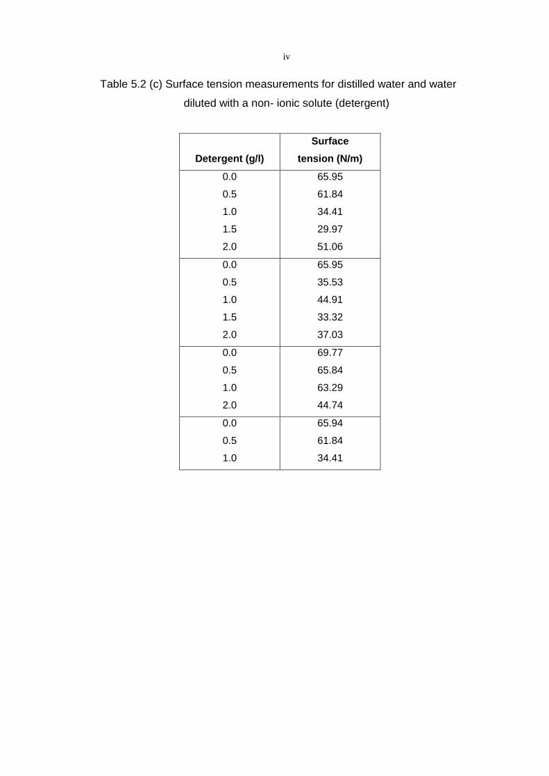
iv
Table 5.2 (c) Surface tension measurements for distilled water and water
diluted with a non- ionic solute (detergent)
Detergent (g/l)
Surface
tension (N/m)
0.0
0.5
1.0
1.5
2.0
65.95
61.84
34.41
29.97
51.06
0.0
0.5
1.0
1.5
2.0
65.95
35.53
44.91
33.32
37.03
0.0
0.5
1.0
2.0
69.77
65.84
63.29
44.74
0.0
0.5
1.0
65.94
61.84
34.41

v
Table 5.3 (a) Results of calibration of psychrometer tips
Molar
solution
48274
48250
48228
Voltage Suction Voltage Suction Voltage Suction
0
0.05
0.5
1.0
1.5
0
0.793
10.14
21.14
26.42
0
0.234
2.281
4.64
7.134
0.493
0.517
8.656
19.82
24.64
0
0.234
2.281
4.64
7.134
0.55
0.518
5.87
-
-
0
0.234
2.281
-
-
Molar
solution
48255
48114
Voltage Suction Voltage Suction
0
0.05
0.5
1.0
1.5
0,529
1.028
9.954
20.141
0
0.234
2.281
4.64
0.5
0.67
9.846
20.87
27.826
0
0.234
2.281
4.64
7.134

vi
y = 0,2339x - 0,0619 R2 = 0,9995
0
1
2
3
4
5
0 20 40T
ota
l su
cti
on
(M
Pa)
Microvolts μV
Thermocouple PSY SN 48225
y = 0,2716x - 0,0821 R2 = 0,9798
012345678
0 10 20 30
To
tal su
cti
on
(M
Pa)
Microvolts μV
Thermocouple PSY SN° 48250
y = 0,3955x - 0,0374 R2 = 0,9973
0
0.5
1
1.5
2
2.5
0 5 10
To
tal su
cti
on
(M
Pa)
Microvolts μV
Thermocouple PSY SN 48228

vii
Figure 5.3 Calibration curves of psychrometers
y = 0,2479x - 0,1021 R2 = 0,991
0
1
2
3
4
5
6
7
8
0 10 20 30
To
tal su
cti
on
(M
Pa
)
Microvolts uV
Thermocouple PSY SN 48114
O
y = 0,253x - 0,1022 R2 = 0,9801
0
1
2
3
4
5
6
7
8
0 10 20 30
To
tal su
cti
on
(M
Pa)
Microvolts μV
Thermocouple PSY SN° 48274

viii
Table 5.3 (b) Total suction values for Limestone Powder
Limestone Powder
0.25 M NaCl 0.50 M NaCl 0.75 M NaCl
Real Mc (%)
Lab Mc (%)
Suction (MPa)
Real Mc (%)
Lab Mc (%)
Suction (MPa)
Real Mc (%)
Lab Mc (%)
Suction (MPa)
1.00 2.00 3.00 4.00 5.00 6.00 7.00 8.00 9.00 10.00
1 2.03 2.87 4.00 4.89 5.75 6.78 7.74 8.86 9.41
ND 4.05 2.71 2.10 1.84 1.74 1.59 1.56 1.50 1.49
1.00 2.00 3.00 4.00 5.00 6.00 7.00 8.00 9.00 10.00
1.22 2.03 2.99 4.04 4.86 5.86 6.70 7.81 8.91 9.52
ND 5.31 3.65 3.39 3.00 2.96 2.95 2.92 2.84 2.73
1.00 2.00 3.00 4.00 5.00 6.00 7.00 8.00 9.00 10.00
1.05 2.06 3.08 4.07 4.93 5.86 6.84 7.84 8.88 9.65
ND 6.20 4.93 4.76 4.40 4.39 4.24 4.23 4.20 3.94
Limestone Powder
1 M NaCl Control 2g/l Detergent
Real Mc (%)
Lab Mc (%)
Suction (MPa)
Real Mc (%)
Lab Mc (%)
Suction (MPa)
Real Mc (%)
Lab Mc (%)
Suction (MPa)
1.00 2.00 3.00 4.00 5.00 6.00 7.00 8.00 9.00 10.00
1.14 2.10 2.96 3.93 4.90 5.93 6.61 7.75 8.66 9.69
ND 7.47 6.44 5.82 5.81 5.68 5.13 5.11 4.99 4.80
1.00 2.00 3.00 4.00 5.00 6.00 7.00 8.00 9.00 10.00
0.83 1.79 2.63 3.30 4.48 5.68 6.66 7.76 8.98 9.83
6.88 3.40 1.88 1.04 0.69 0.46 0.36 0.33 0.20 0.28
1.00 2.00 3.00 4.00 5.00 6.00 7.00 8.00 9.00 10.00
1.14 1.81 2.86 3.80 4.68 5.71 6.90 7.59 8.73 9.66
ND 3.57 1.36 0.942 0.846 0.484 0.429 0.38 0.293 0.361
Lab Mc: Moisture content of specimen measured in the laboratory Real Mc: Target moisture content

ix
Table 5.3 (c) Total suction values for Quartz Powder
Quartz Powder
0.25 M NaCl 0.50 M NaCl 0.75 M NaCl
Real Mc (%)
Lab Mc (%)
Suction (MPa)
Real Mc (%)
Lab Mc (%)
Suction (MPa)
Real Mc (%)
Lab Mc (%)
Suction (MPa)
1.00 2.00 3.00 4.00 5.00 6.00 7.00 8.00 9.00 10.00
0.79 1.80 2.95 3.76 4.75 5.88 6.73 7.61 8.72 9.82
2.80 1.88 1.82 1.65 1.74 1.61 1.43 1.41 1.40 1.39
1.00 2.00 3.00 4.00 5.00 6.00 7.00 8.00 9.00 10.00
0.90 1.81 2.76 3.59 4.62 5.63 6.72 7.63 8.50 9.63
3.86 3.72 3.33 3.33 3.27 2.91 2.88 2.78 2.75 2.71
1.00 2.00 3.00 4.00 5.00 6.00 7.00 8.00 9.00 10.00
0.81 1.84 2.83 2.77 4.78 5.55 6.58 7.47 8.52 9.42
5.89 5.08 4.88 4.51 4.28 4.40 4.28 4.25 4.11 4.00
Quartz Powder
1 M NaCl Control 2g/l Detergent
Real Mc (%)
Lab Mc (%)
Suction (MPa)
Real Mc (%)
Lab Mc (%)
Suction (MPa)
Real Mc (%)
Lab Mc (%)
Suction (MPa)
1.00 2.00 3.00 4.00 5.00 6.00 7.00 8.00 9.00 10.00
0.85 1.76 2.78 3.88 4.60 5.55 6.62 7.57 8.53 9.23
7.61 6.58 5.90 5.56 5.44 5.06 5.26 5.05 4.96 5.55
1.00 2.00 3.00 4.00 5.00 6.00 7.00 8.00 9.00 10.00
0.69 1.70 2.61 3.51 4.72 5.48 6.42 7.37 8.65 9.32
0.960 0.815 0.380 0.140 0.220 0.072 0.118 0.137 0.125 0.152
1.00 2.00 3.00 4.00 5.00 6.00 7.00 8.00 9.00 10.00
0.90 1.95 2.96 3.97 4.50 5.60 6.80 7.78 8.76 9.87
0.55 0.32 0.27 0.18 0.19 0.14 0.12 0.13 0.08 0.062
Lab Mc: Moisture content of specimen measured in the laboratory Real Mc: Target moisture content

x
Table 5.3 (d) Total suction values for Fine Glass Beads
Fine Glass Beads
0.25 M NaCl 0.50 M NaCl 0.75 M NaCl
Real Mc (%)
Lab Mc (%)
Suction (MPa)
Real Mc (%)
Lab Mc (%)
Suction (MPa)
Real Mc (%)
Lab Mc (%)
Suction (MPa)
1.00 2.00 3.00 4.00 5.00 6.00 7.00 8.00 9.00 10.00
0.91 1.90 2.92 3.82 4.71 5.74 6.59 7.71 8.54 9.60
4.21 2.63 2.17 2.03 1.86 1.78 1.65 1.65 1.65 1.65
1.00 2.00 3.00 4.00 5.00 6.00 7.00 8.00 9.00 10.00
0.89 1.80 2.82 3.75 4.62 5.61 6.58 7.51 8.30 9.48
5.44 4.25 3.49 3.33 3.11 3.05 3.03 3.05 3.00 2.91
1.00 2.00 3.00 4.00 5.00 6.00 7.00 8.00 9.00 10.00
1.08 1.83 2.63 3.77 4.56 5.59 6.56 7.60 8.39 9.23
5.87 4.88 4.67 4.61 4.51 4.36 4.34 4.36 4.34 4.07
Fine Glass Beads
1 M NaCl Control 2g/l Detergent
Real Mc (%)
Lab Mc (%)
Suction (MPa)
Real Mc (%)
Lab Mc (%)
Suction (MPa)
Real Mc (%)
Lab Mc (%)
Suction (MPa)
1.00 2.00 3.00 4.00 5.00 6.00 7.00 8.00 9.00 10.00
0.98 1.79 2.67 3.61 4.52 5.52 6.33 7.41 8.36 9.07
7.30 6.72 6.39 6.18 5.89 5.86 5.79 5.58 5.80 5.40
1.00 2.00 3.00 4.00 5.00 6.00 7.00 8.00 9.00 10.00
0.98 1.87 2.83 3.92 4.88 5.77 6.98 7.78 8.86 9.96
2.55 1.40 0.92 0.70 0.69 0.56 0.49 0.43 0.36 0.35
1.00 2.00 3.00 4.00 5.00 6.00 7.00 8.00 9.00 10.00
0.90 2.03 2.75 3.77 4.69 5.79 6.62 7.68 8.59 9.43
2.64 1.34 0.767 0.749 0.644 0.485 0.429 0.383 0.296 0.332
Lab Mc: Moisture content of specimen measured in the laboratory Real Mc: Target moisture content

xi
Table 5.4 (a) (i) Calibration of triaxial cell and pore pressure transducers
Cell 1
Cell Height Actual Difference Volume
Change
PWR
0
50
100
150
200
300
400
500
600
650
81.0
79.5
78.0
76.8
75.4
72.8
70.2
67.6
65.0
63.0
78.5
77.0
75.5
74.3
72.9
70.3
67.7
65.1
62.5
60.5
0.0
1.5
3.0
4.2
5.6
8.2
10.8
13.4
16.0
18.0
0.0
0.612
1.224
1.7136
2.2848
3.3456
4.4064
5.4672
6.528
7.344
76
-23
-130
-158
-321
-527
-735
-935
-1145
-1240
0
1
2
3
4
5
6
7
8
0 100 200 300 400 500 600 700
Vo
lum
e c
ha
ng
e(c
c)
Cell Pressure (kPa)
Cell pressure Vs Volume change cell 1 TM 1

xii
Cell 2
Cell Height Actual Difference Volume
Change
PWR
0
50
100
150
200
300
400
500
600
650
82.1
80.4
78.8
77.5
76.1
73.4
70.7
67.9
65.2
63.9
69.8
68.1
66.5
65.2
63.8
61.1
58.4
55.6
52.9
51.6
0.0
1.7
3.3
4.6
6.0
8.2
11.4
14.2
16.9
18.2
0.0
0.6936
1.3464
1.8768
2.448
3.5496
4.6512
5.7936
6.8952
7.4256
0
102
200
305
407
608
810
1014
1215
1317
y = -0.4868x + 44.889 R² = 0.998
0
100
200
300
400
500
600
700
-1500 -1000 -500 0 500
Tru
e P
ressu
re (
kP
a)
PWR readout (kPa)
True Pressure Vs PWR readout Cell 1

xiii
0
1
2
3
4
5
6
7
8
0 100 200 300 400 500 600 700
Vo
lum
e c
han
ge (
cc)
Cell Pressure (kPa)
Cell pressure Vs Volume change cell 2 TM 2
y = 0.4935x R² = 1
-100
0
100
200
300
400
500
600
700
0 200 400 600 800 1000 1200 1400
Ce
ll p
ress
ure
(kP
a)
PWR readout (kPa)
Cell pressure Vs PWR readout Cell 2 TM 2

xiv
Cell 3
Cell Height Actual Difference Volume
Change
PWR
0
50
100
150
200
300
400
500
600
86.9
85.4
84.0
82.4
81.0
78.0
75.0
72.0
69.0
63.3
62.8
60.4
58.8
57.4
54.4
51.4
48.4
45.4
0.0
1.5
2.9
4.5
5.9
8.9
11.9
14.9
17.9
0.0
0.612
1.836
1.7136
2.4072
3.6312
4.8552
6.0792
7.3032
10
50
100
150
200
300
400
500
600.5
0
1
2
3
4
5
6
7
8
9
0 100 200 300 400 500 600
Vo
lum
e c
ha
ng
e (
cc)
Cell pressure (kPa)
Cell pressure Vs Volume change cell 3 TM 3
Series1
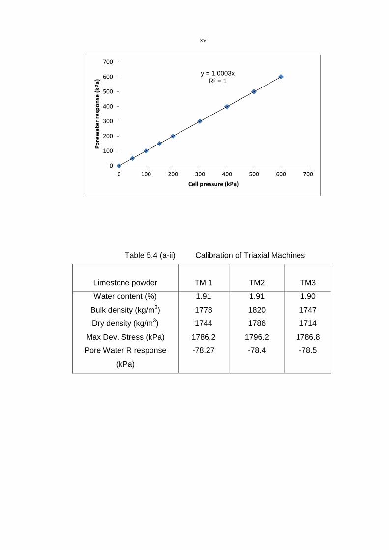
xv
Table 5.4 (a-ii) Calibration of Triaxial Machines
Limestone powder
TM 1
TM2
TM3
Water content (%)
Bulk density (kg/m3)
Dry density (kg/m3)
Max Dev. Stress (kPa)
Pore Water R response
(kPa)
1.91
1778
1744
1786.2
-78.27
1.91
1820
1786
1796.2
-78.4
1.90
1747
1714
1786.8
-78.5
y = 1.0003x R² = 1
0
100
200
300
400
500
600
700
0 100 200 300 400 500 600 700
Po
rew
ate
r re
spo
nse
(kP
a)
Cell pressure (kPa)

xvi
Table 5.4(b) Results of triaxial strength tests and suctions for limestone powder
Limestone Powder Control
Moisture content (%)
PWR (kPa)
Suction (kPa)
Max. Dev. Stress (kPa)
Bulk Density (kg/m3)
Dry Density (kg/m3)
2 4 6 8 10
-78.03 -71.00 -55.27 -63.87 -8.97
278.03 271.00 255.27 263.87 208.97
1765.51 1609.00 1283.30 1047.01 1010.36
1868 1954 1838 1784 1801
1834 1882 1741 1667 1642
0.25 M NaCl Limestone Powder
Moisture content (%)
PWR (kPa)
Suction (kPa)
Max. Dev. Stress (kPa)
Bulk Density (kg/m3)
Dry Density (kg/m3)
2 4 6 8 10
-77.55 -75.00 -69.73 -28.00 -55.16
277.55 275.00 269.73 228.00 255.16
1876.87 1571.51 1293.76 1053.73 936.51
1885 1874 1852 1818 1840
1832 1797 1711 1679 1669
0.50 M NaCl Limestone Powder
Moisture content (%)
PWR (kPa)
Suction (kPa)
Max. Dev. Stress (kPa)
Bulk Density (kg/m3)
Dry Density (kg/m3)
2 4 6 8 10
-78.52 -26.26 -38.00 -70.22 10.00
278.52 226.26 238.00 270.22 190.00
1845.30 1448.14 1367.52 1053.63 952.80
1854 1875 1902 1784 1762
1812 1775 1796 1658 1593
0.75 M NaCl Limestone Powder
Moisture content (%)
PWR (kPa)
Suction (kPa)
Max. Dev. Stress (kPa)
Bulk Density (kg/m3)
Dry Density (kg/m3)
2 4 6 8 10
-70.22 -45.74 -33.50 -22.79 -13.50
270.22 245.74 233.50 222.79 213.50
1763.72 1569.29 1304.88 1184.68 969.89
1867 1859 1834 1884 1848
1832 1785 1725 1743 1684

xvii
Continuation Table 5.4(b) results of triaxial strength tests and suctions for Limestone Powder
1 M NaCl Limestone Powder
Moisture content (%)
PWR (kPa)
Suction (kPa)
Max. Dev. Stress (kPa)
Bulk Density (kg/m3)
Dry Density (kg/m3)
2 4 6 8 10
-78.03 -74.13 -50.00 -44.00 -31.62
278.03 274.13 250.00 244.00 231.62
1811.66 1554.52 1204.91 1265.76 1069.16
1872 1899 1812 1830 1783
1829 1825 1700 1699 1628
2g/l Detergent Limestone Powder
Moisture content (%)
PWR (kPa)
Suction (kPa)
Max. Dev. Stress (kPa)
Bulk Density (kg/m3)
Dry Density (kg/m3)
2 4 6 8 10
-78.08 -40.60 -53.61 14.00 -38.27
276.08 240.60 253.61 186.00 238.27
1683.06 1564.04 1085.85 1143.00 914.11
1921 1898 2017 1758 1754
1868 1821 1821 1618 1592
PWR: Pore water response Max. Dev. Stress: Maximum deviator stress

xviii
Table 5.4 (c) results of triaxial strength tests and suctions for Quartz Powder
Quartz Powder Control
Moisture content (%)
PWR (kPa)
Suction (kPa)
Max. Dev. Stress
Bulk Density (kg/m3)
Dry Density (kg/m3)
2 4 6 8 10
176 186 190 190 192
24.00 14.00 10.00 10.00 08.00
1439 1500 1382 1308 1098
1834 1994 1939 1843 1847
1803 1926 1836 1705 1689
0.25 M NaCl Quartz Powder
Moisture content (%)
PWR (kPa)
Suction (kPa)
Max. Dev. Stress
Bulk Density (kg/m3)
Dry Density (kg/m3)
2 4 6 8 10
191.14 192.50 193.00 192.50 199.70
08.86 07.50 07.00 07.50 00.30
1342.20 1268.59 1103.38 1105.40 1076.70
1811 1821 1830 1808 1898
1760 1742 1720 1683 1681
0.50 M NaCl Quartz Powder
Moisture content (%)
PWR (kPa)
Suction (kPa)
Max. Dev. Stress
Bulk Density (kg/m3)
Dry Density (kg/m3)
2 4 6 8 10
185.21 182.77 189.62 190.59 195.00
14.79 17.23 10.38 09.41 05.00
1256.14 1274.66 1283.79 1130.59 1077.37
1990 1832 1869 1815 1722
1892 1632 1752 1677 1546
0.75 M NaCl Quartz Powder
Moisture content (%)
PWR (kPa)
Suction (kPa)
Max. Dev. Stress
Bulk Density (kg/m3)
Dry Density (kg/m3)
2 4 6 8 10
178.00 192.06 191.00 193.53 195.4
22.00 15.00 9.00 6.47 5.41
1502.70 1311.63 1237.32 1193.47 1099.78
1832 1884 1830 1760 1862
1799 1816 1725 1632 1711

xix
Continuation Table 5.4 (c) results of triaxial strength tests and suctions for Quartz Powder.
1 M NaCl Quartz Powder
Moisture content
(%)
PWR (kPa)
Suction (kPa)
Max. Dev.
Stress
Bulk Density (kg/m3)
Dry Density (kg/m3)
2 4 6 8 10
169.00 188.00 188.00 179.00 199.00
31.00 12.00 12.00 21.00 1.00
1376.00 1288.00 1230.34 1052.36 1024.53
1827 1785 1805 1770 1749
1799 1816 1725 1632 1570
2g/l Detergent Quartz Powder
Moisture content
(%)
PWR (kPa)
Suction (kPa)
Max. Dev.
Stress
Bulk Density (kg/m3)
Dry Density (kg/m3)
2 4 6 8 10
197.42 194.63 193.00 192.05 192.53
2.58 5.37 7.00 7.95 7.47
1320.80 1211.30 1174.17 1097.72 1129.96
2075 2083 1844 1749 185 6
1841 2000 1748 1628 1697
PWR: Pore water response Max. Dev. Stress: Maximum deviator stress

xx
Table 5.4(d) results of triaxial strength tests and suctions for Fine Glass Beads
Fine Glass Beads Control
Moisture content (%)
PWR (kPa)
Suction (kPa)
Max. Dev. Stress
Bulk Density (kg/m3)
Dry Density (kg/m3)
2 4 6 8 10
195.96 191.50 195.13 188.43 191.50
4.04 8.50 8.47
11.57 8.50
578.90 590.34 586.16 582.30 516.60
1776 1780 1670 2070 1768
1741 1719 1587 1920 1622
0.25 M NaCl Fine Glass Beads
Moisture content (%)
PWR (kPa)
Suction (kPa)
Max. Dev. Stress
Bulk Density (kg/m3)
Dry Density (kg/m3)
2 4 6 8 10
193.03 193.00 192.50 192.05 194.48
6.97 7.00 7.50 7.95 5.52
611.22 674.69 673.41 654.33 604.38
1776 1727 1697 2067 1783
1742 1664 1601 1928 1627
0.50 M NaCl Fine Glass Beads
Moisture content (%)
PWR (kPa)
Suction (kPa)
Max. Dev. Stress
Bulk Density (kg/m3)
Dry Density (kg/m3)
2 4 6 8 10
191.56 193.51 198.50 197.56 192.54
8.44 -6.49 1.50 2.44 7.46
833.86 694.63 651.68 618.47 687.14
1732 1723 1690 1692 1678
1700 1661 1611 1579 1520
0.75 M NaCl Fine Glass Beads
Moisture content (%)
PWR (kPa)
Suction (kPa)
Max. Dev. Stress
Bulk Density (kg/m3)
Dry Density (kg/m3)
2 4 6 8 10
184.24 184.79 192.5
193.52 195.42
15.76 15.21 7.50 6.48 4.58
641.35 675.00 757.61 731.22 605.63
1790 1782 1690 1750 1708
1755 1724 1611 1629 1562

xxi
Continuation Table 5.4(d) results of triaxial strength tests and suctions for Fine Glass Beads
1 M NaCl Fine Glass Beads
Moisture content
(%)
PWR (kPa)
Suction (kPa)
Max. Dev.
Stress
Bulk Density (kg/m3)
Dry Density (kg/m3)
2 4 6 8
10
189.61 188.59 192.50 195.00 155.07
10.39 11.41 7.50 5.00
44.93
766.45 742.28 739.24 726.27 673.83
1872 1899 1812 1830 1783
1829 1825 1700 1699 1628
2g/l Detergent Fine Glass Beads
Moisture content
(%)
PWR (kPa)
Suction (kPa)
Max. Dev.
Stress
Bulk Density (kg/m3)
Dry Density (kg/m3)
2 4 6 8
10
190.10 188.14 197.00 197.40 198.00
9.90 11.86 3.00 2.60 2.00
579.36 586.26 551.99 660.39 571.83
1715 1698 1671 1813 1656
1686 1641 1582 1694 1546
PWR: Pore water response Max. Dev. Stress: Maximum deviator stress

xxii
Table 5.4 (e) Results of s-t parameters Limestone Powder
Limestone Powder- Control
Mc (%)
½(σ1-σ3) (kPa)
½(σ1+σ3) (kPa)
½(σ1+σ3)-ua (kPa)
½(σ1+σ3)-uw
(kPa)
φ φ'
2 4 6 8 10
882.76 804.50 641.65 523.51 505.18
1382.76 1304.50 1141.65 1023.51 1005.18
1182.76 1104.50 941.65 823.51 805.18
1460.79 1375.50 1196.92 1087.38 1014.15
48.30 46.77 42.98 39.49 38.88
37.20 35.81 32.43 28.79 29.89
Limestone Powder- 0.25 M NaCl
Mc (%)
½(σ1-σ3) (kPa)
½(σ1+σ3) (kPa)
½(σ1+σ3)-ua (kPa)
½(σ1+σ3)-uw
(kPa)
φ φ'
2 4 6 8 10
938.43 785.76 646.88 526.86 468.26
1438.43 1285.76 1146.88 1026.86 968.26
1238.43 1085.76 946.88 826.86 768.26
1515.98 1360.76 1216.61 1054.86 1023.42
49.29 46.38 43.11 39.60 37.57
38.26 35.29 32.14 29.98 27.24
Limestone Powder- 0.50 M NaCl
Mc (%)
½(σ1-σ3) (kPa)
½(σ1+σ3) (kPa)
½(σ1+σ3)-ua (kPa)
½(σ1+σ3)-uw
(kPa)
φ φ'
2 4 6 8 10
922.65 724.07 683.76 526.82 476.40
1422.65 1224.07 1183.76 1026.82 976.40
1222.65 1024.07 983.76 826.82 776.40
1501.17 1250.33 1221.76 1097.04 966.40
49.02 45.02 44.05 39.60 37.87
37.94 35.41 34.05 28.71 29.55
Limestone Powder- 0.75 M NaCl
Mc (%)
½(σ1-σ3) (kPa)
½(σ1+σ3) (kPa)
½(σ1+σ3)-ua (kPa)
½(σ1+σ3)-uw
(kPa)
φ φ'
2 4 6 8 10
881.86 784.65 652.44 592.34 484.95
1381.86 1284.65 1152.44 1092.34 984.95
1181.86 1084.65 952.44 892.34 784.95
1452.08 1330.38 1185.94 1115.12 998.45
48.28 46.36 43.26 41.61 38.18
37.41 36.16 33.39 32.10 29.07
Limestone Powder- 1M NaCl
Mc (%)
½(σ1-σ3) (kPa)
½(σ1+σ3) (kPa)
½(σ1+σ3)-ua (kPa)
½(σ1+σ3)-uw
(kPa)
φ φ'
2 4 6 8 10
905.83 777.26 602.45 632.88 534.58
1405.83 1277.26 1102.45 1132.88 1034.58
1205.83 1077.26 902.45 932.88 834.58
1483.86 1351.39 1152.45 1176.88 1066.20
48.72 46.20 41.90 42.74 39.85
37.64 35.13 31.53 32.55 30.11

xxiii
Continuation of Table 5.4 (e) Results of s-t parameters Limestone Powder
Limestone Powder-2g/l Detergent
Mc (%)
½(σ1-σ3) (kPa)
½(σ1+σ3) (kPa)
½(σ1+σ3)-ua (kPa)
½(σ1+σ3)-uw
(kPa)
φ φ'
2 4 6 8 10
841.53 782.02 542.92 571.50 457.05
1341.53 1282.02 1042.92 1071.50 957.05
1141.53 1082.02 842.92 871.50 757.05
1417.61 1322.62 1096.54 1057.50 995.32
47.52 46.30 40.12 41.00 37.16
36.43 36.27 29.69 32.73 27.35

xxiv
Table 5.4 (f) Results of s-t parameters Quartz Powder
Quartz Powder- Control
Mc (%)
½(σ1-σ3) (kPa)
½(σ1+σ3) (kPa)
½(σ1+σ3)-ua (kPa)
½(σ1+σ3)-uw
(kPa)
φ φ'
2 4 6 8 10
719.50 750.00 691.00 654.00 549.00
1219.50 1250.00 1191.00 1154.00 1049.00
1019.50 1050.00 991.00 954.00 849.00
1043.50 1064.00 1001.00 964.00 857.00
44.91 45.61 44.23 43.30 40.31
43.61 44.84 43.68 42.74 39.86
Quartz Powder- 0.25 M NaCl
Mc (%)
½(σ1-σ3) (kPa)
½(σ1+σ3) (kPa)
½(σ1+σ3)-ua (kPa)
½(σ1+σ3)-uw
(kPa)
φ φ'
2 4 6 8 10
671.10 634.29 551.69 552.70 538.35
1171.10 1134.29 1051.69 1052.70 1038.35
971.10 934.29 851.69 852.70 838.35
979.96 941.79 858.69 860.20 838.65
43.74 42.78 40.39 40.42 39.97
43.24 42.36 40.00 40.00 39.96
Quartz Powder- 0.50 M NaCl
Mc (%)
½(σ1-σ3) (kPa)
½(σ1+σ3) (kPa)
½(σ1+σ3)-ua (kPa)
½(σ1+σ3)-uw
(kPa)
φ φ'
2 4 6 8 10
628.07 637.33 641.89 565.29 538.68
1128.07 1137.33 1141.89 1065.29 1038.68
928.07 937.33 941.89 865.29 838.68
921.66 954.56 933.37 874.71 843.68
42.61 42.86 42.98 40.81 39.98
42.98 41.91 43.47 40.28 39.70
Quartz Powder- 0.75 M NaCl
Mc (%)
½(σ1-σ3) (kPa)
½(σ1+σ3) (kPa)
½(σ1+σ3)-ua (kPa)
½(σ1+σ3)-uw
(kPa)
φ φ'
2 4 6 8 10
751.35 655.81 618.66 596.73 550.12
1251.35 1155.81 1118.66 1096.73 1050.12
1051.35 955.81 918.66 896.73 850.12
1073.35 963.76 927.66 903.20 843.72
45.64 43.35 42.35 41.74 40.34
44.45 42.90 41.85 41.37 40.71
Quartz Powder- 1M NaCl
Mc (%)
½(σ1-σ3) (kPa)
½(σ1+σ3) (kPa)
½(σ1+σ3)-ua (kPa)
½(σ1+σ3)-uw
(kPa)
φ φ'
2 4 6 8 10
688.00 644.00 615.17 526.18 512.27
1188.00 1144.00 1115.17 1026.18 1012.27
988.00 944.00 915.17 826.18 812.27
1019.00 956.00 927.17 847.18 813.27
44.16 43.04 42.26 39.58 39.12
42.49 42.37 41.59 38.42 39.06

xxv
Continuation of Table 5.4(f) Results of s-t parameters Quartz Powder
Quartz Powder-2g/l Detergent
Mc (%)
½(σ1-σ3) (kPa)
½(σ1+σ3) (kPa)
½(σ1+σ3)-ua (kPa)
½(σ1+σ3)-uw
(kPa)
φ φ'
2 4 6 8 10
660.40 605.65 587.09 548.8
564.98
1160.40 1105.65 1087.09 1048.86 1064.98
960.40 905.65 887.09 848.86 864.98
962.98 911.02 894.09 856.81 857.97
43.46 41.99 41.46 40.31 40.80
43.32 41.69 41.06 39.86 41.21

xxvi
Table 5.4 (g) Results of s-t parameters Fine Glass Beads
Fine Glass Beads- Control
Mc (%)
½(σ1-σ3) (kPa)
½(σ1+σ3) (kPa)
½(σ1+σ3)-ua (kPa)
½(σ1+σ3)-uw
(kPa)
φ φ'
2 4 6 8
10
289.45 295.17 293.08 291.15 258.30
789.45 795.17 793.08 791.15 758.30
589.45 595.17 593.08 591.15 558.30
593.49 603.67 597.95 602.72 566.80
29.42 29.75 29.63 29.52 29.57
29.20 29.29 29.36 28.90 27.12
Fine Glass Beads - 0.25 M NaCl
Mc (%)
½(σ1-σ3) (kPa)
½(σ1+σ3) (kPa)
½(σ1+σ3)-ua (kPa)
½(σ1+σ3)-uw
(kPa)
φ φ'
2 4 6 8
10
305.61 337.35 336.70 327.17 302.19
805.61 837.35 836.70 827.17 802.19
605.61 637.35 636.70 627.17 602.19
612.58 644.35 644.20 635.12 596.38
30.32 31.97 31.94 31.46 30.14
29.94 31.59 31.53 31.02 30.46
Fine Glass Beads - 0.50 M NaCl
Mc (%)
½(σ1-σ3) (kPa)
½(σ1+σ3) (kPa)
½(σ1+σ3)-ua (kPa)
½(σ1+σ3)-uw
(kPa)
φ φ'
2 4 6 8
10
416.93 347.32 325.84 309.24 343.57
916.93 847.32 825.84 809.24 843.57
716.93 647.32 625.84 609.24 643.57
725.37 431.02 627.34 611.68 651.03
35.58 32.47 31.39 30.52 32.28
35.10 *
31.31 30.38 31.87
Fine Glass Beads - 0.75 M NaCl
Mc (%)
½(σ1-σ3) (kPa)
½(σ1+σ3) (kPa)
½(σ1+σ3)-ua (kPa)
½(σ1+σ3)-uw
(kPa)
φ φ'
2 4 6 8
10
320.68 337.50 378.80 365.61 302.81
820.68 837.50 878.80 865.61 802.81
620.68 637.50 678.80 665.61 602.81
636.44 652.71 686.30 672.09 423.70
31.12 31.98 33.94 33.33 30.17
30.27 31.15 33.52 32.97 45.64
Fine Glass Beads - 1M NaCl
Mc (%)
½(σ1-σ3) (kPa)
½(σ1+σ3) (kPa)
½(σ1+σ3)-ua (kPa)
½(σ1+σ3)-uw
(kPa)
φ φ'
2 4 6 8 10
383.23 371.14 369.62 363.14 336.92
883.23 871.14 869.62 863.14 836.92
683.23 671.14 669.62 663.14 836.92
693.62 682.54 677.12 668.14 681.85
34.14 33.59 33.52 33.22 31.95
33.56 32.96 33.1 32.94 29.63

xxvii
Continuation of Table 5.4 (g) results of s-t parameters Fine Glass Beads
Fine Glass Beads -2g/l Detergent
Mc (%)
½(σ1-σ3) (kPa)
½(σ1+σ3) (kPa)
½(σ1+σ3)-ua (kPa)
½(σ1+σ3)-uw
(kPa)
φ φ'
2 4 6 8
10
289.68 293.13 275.99 330.19 285.92
789.68 793.13 755.99 830.19 785.92
589.68 593.13 575.99 630.19 585.92
559.58 604.99 578.99 623.48 587.92
29.44 29.63 28.65 31.61 29.22
28.91 29.00 28.48 31.99 29.11

xxviii
Table 5.5 (a) Consolidated drained tests for Limestone powder
Limestone powder
Control with pure
water
1M NaCl mix Water
BP
1M NaCl mix. Salt BP
Detergent mix. Water
BP
Detergent mix.
Detergent BP
Peak Max. Deviator stress (kPa)
Cell
Pressure (kPa)
Back
pressure (kPa)
PWR (kPa)
Bulk density
(kg/m3)
Dry density (kg/m3)
821
450
150
154
1919
1573
821
450
150
149
1815
1504
763
500
200
197
1791
1481
772
500
200
197.5
1746
1450
819
500
200
197
1752
1453
BP: Backwater Pressure PWR: Porewater Response

xxix
Table 5.5 (b) Consolidated drained tests for Quartz powder
Quartz powder
Control with pure
water
1M NaCl mix Water
BP
1M NaCl mix. Salt BP
Detergent mix. Water
BP
Detergent mix.
Detergent BP
Peak Max.
Deviator
stress (kPa)
Cell
Pressure
(kPa)
Back
pressure
(kPa)
PWR
(kPa)
Bulk density
(kg/m3)
Dry density
(kg/m3)
1151
400
100
106.5
2050
1622
1168.5
400
100
100.5
1771
1490
1155.2
400
100
198
1783
1516
1155
450
150
153.5
1827
1493
1138
400
100
97.5
1742
1451
BP: Backwater Pressure PWR: Porewater Response

xxx
Table 5.5 (c) Consolidated drained tests for Fine Glass beads
Fine Glass beads
Control with pure
water
1M NaCl mix Water
BP
1M NaCl mix. Salt BP
Detergent mix. Water
BP
Detergent mix.
Detergent BP
Peak Max. Deviator
stress (kPa)
Cell Pressure
(kPa)
Back pressure
(kPa)
PWR (kPa)
Bulk density
(kg/m3)
Dry density (kg/m3)
464.32
400
100
116.5
1582
1263
406.32
400
100
104
1559
1229
412.83
400
100
104
1593
1271
473
400
100
99
1529
1177
398
400
100
99
1662
1308
BP: Backwater Pressure PWR: Porewater Response

xxxi
Table 5.5 d. The φ´ values of the consolidated drained tests.
Soil Mix 𝜑'
Limestone Powder
water-water
salt-salt
salt-water
det-det
det-water
35.5°
35.9°
35.3°
35.1°
34.2°
Quartz powder
water-water
salt-salt
salt-water
det-det
det-water
41.5°
47.8°
41.4°
40.8°
41.4°
Glass beads
water-water
salt-salt
salt-water
det-det
det-water
26.8°
24.3°
24.0°
23.5°
26.1°

xxxii
Table 5.6 Shear strength test results of limestone powder in different saturated solutions then exposed to atmospheres of distilled water, 1M NaCl and
detergent. Initial water content 6%.Total exposure time 6 months
After 3 months exposure After 6 months exposure
Soil Mixed
with
Dried over
saturated solutions
Peak Max. dev.
Stress (kPa)
Water content
(%)
ρb (kg/m
3)
ρd (kg/m
3)
Re- Exposed
to
Max dev.
Stress (kPa)
Water content
(%)
ρb (kg/m
3)
ρd (kg/m
3
)
Water
K2SO4
1480 0.97 1794 1776 water NaCl Det
- 1876 1345
- 1.21 1.45
- 1754 1755
- 1734 1730
ZnSO4 1111 1.44 1816 1790 Water NaCl Det
1593 -
1714
1.48 -
2.76
1771 -
1773
1745 -
1725
Na2SO4 1176 3.97 1869 1770 Water NaCl Det
1342 1924 1299
1.19 1.41 1.53
1775 1742 1754
1754 1723 1728
1 M NaCl
K2SO4
1068 4.48 1931 1848 Water NaCl Det
1181 -
903
6.23 -
7.69
2024 -
1866
1905 -
1733
ZnSO4 - - - - Water NaCl Det
1080 1078 1034
6.18 3.86 10.6
1879 1812 2094
1786 1739 1894
Na2SO4 1395 2.02 1774 1739 Water NaCl Det
1017 1203
-
8.46 1.08
-
1923 1851
-
1773 1782
-
2g/L Detergen
t
K2SO4
1538 1.04 1753 1735 Water NaCl Det
1213 1010 1271
2.04 4.62 0.84
1793 1873 1744
1757 1790 1730
ZnSO4 1372 1.57 1798 1770 Water NaCl Det
1334 1361 1208
2.88 1.18 1.95
1828 1759 1738
1777 1873 1712
Na2SO4 1677 0.75 1729 1716 Water NaCl Det
1248 1454 1326
1.22 1.13 1.53
1749 1731 1738
1728 1712 1712