submitted to ieee transactions on … · cyclostationary random processes ... it is well known that...

arX

iv:1

304.

7375

v1 [

cs.IT

] 27

Apr

201

3SUBMITTED TO IEEE TRANSACTIONS ON INFORMATION THEORY (VER 1.0) 1

Asymptotic FRESH Properizer for Block

Processing of Improper-Complex Second-Order

Cyclostationary Random Processes

Jeongho Yeo and Joon Ho ChoMember, IEEE

Abstract

In this paper, the block processing of a discrete-time (DT) improper-complex second-order cyclosta-

tionary (SOCS) random process is considered. In particular, it is of interest to find a pre-processing oper-

ation that enables computationally efficient near-optimalpost-processing. An invertible linear-conjugate

linear (LCL) operator named the DT FREquency Shift (FRESH) properizer is first proposed. It is

shown that the DT FRESH properizer converts a DT improper-complex SOCS random process input

to an equivalent DT proper-complex SOCS random process output by utilizing the information only

about the cycle period of the input. An invertible LCL block processing operator named the asymptotic

FRESH properizer is then proposed that mimics the operationof the DT FRESH properizer but processes

a finite number of consecutive samples of a DT improper-complex SOCS random process. It is shown

that the output of the asymptotic FRESH properizer is not proper but asymptotically proper and that its

frequency-domain covariance matrix converges to a highly-structured block matrix with diagonal blocks

as the block size tends to infinity. Two representative estimation and detection problems are presented

to demonstrate that asymptotically optimal low-complexity post-processors can be easily designed by

exploiting these asymptotic second-order properties of the output of the asymptotic FRESH properizer.

Index Terms

Asymptotic analysis, complexity reduction, improper-complex random process, properization, second-

order cyclostationarity

The material in this paper was presented in part at the IEEE Military Communications Conference (MILCOM), Orlando, FL,

29 Oct.-1 Nov. 2012 and in part at the IEEE Wireless Communications and Networking Conference (WCNC), Shanghai, China,

7-10 Apr. 2013.

The authors are with the Department of Electrical Engineering, Pohang University of Science and Technology (POSTECH),

Pohang, Gyeongbuk 790-784, Korea (e-mail:yjh2304, [email protected]).

http://arxiv.org/abs/1304.7375v1

2 SUBMITTED TO IEEE TRANSACTIONS ON INFORMATION THEORY (VER 1.0)

I. INTRODUCTION

It is well known that the complex envelope of a real-valued bandpass wide-sense stationary

(WSS) random process is proper, i.e., its complementary auto-covariance (a.k.a. the pseudo-

covariance) function vanishes [1]. However, there are a lotof important improper-complex

random processes that do not have vanishing complementary auto-covariance functions [2]–

[4]. For example, the complex envelope of a real-valued bandpass nonstationary signal is not

necessarily proper and even the complex envelope of a real-valued bandpass WSS signal becomes

improper in the presence of the imbalance between its in-phase and quadrature components [5].

In order to fully capture the statistical properties of a complex-valued signal, including all the

second-order statistics, the filtering of augmented signals has been proposed. This so-called

widely linear (WL) filtering processes either the signal augmented by its complex conjugate or

the real part of the signal augmented by the imaginary part [5], [6], where the former is referred

to as the linear-conjugate linear (LCL) filtering [7].

On the other hand, many digitally modulated signals are wellmodeled by wide-sense cyclo-

stationary (WSCS) random processes [8], [9], whose complexenvelopes possess periodicity in

all variables of the mean and the auto-covariance functions. To efficiently extract the correlation

structure of a WSCS random process in the time and the frequency domains, the translation series

representation (TSR) and the harmonic series representation (HSR) are proposed [10], which are

linear periodically time-varying (PTV) processings. Using these representations, it is shown [10]

that a proper-complex WSCS scalar random process can be converted to an equivalent proper-

complex WSS vector random process. Such second-order structure of a proper-complex WSCS

random process has long been exploited in the design of many communications and signal

processing systems including presence detectors [11], [12], estimators [13]–[15], and optimal

transceivers [16]–[18] under various criteria.

The complex envelopes of the majority of digitally modulated signals are proper and WSCS.

However, as well documented in [5], there still remain many other digitally modulated signals

such as pulse amplitude modulation (PAM), offset quaternary phase-shift keying (OQPSK), and

Gaussian minimum shift keying (GMSK), that are not only improper-complex WSCS but also

second-order cyclostationary (SOCS) [19], i.e., the complementary auto-covariance function is

also periodic in all its variables with the same period as themean and the auto-covariance

SUBMITTED TO IEEE TRANSACTIONS ON INFORMATION THEORY (VER 1.0) 3

functions. To exploit both cyclostationarity and impropriety, the LCL FREquency Shift (FRESH)

filter has been proposed in [20] that combines signal augmentation and linear PTV processing.

Recently, another LCL PTV operator called the properizing FRESH (p-FRESH) vectorizer is

proposed in [19], [21] by non-trivially extending the HSR. The p-FRESH vectorizer converts

an improper-complexSOCS scalar random process to an equivalentproper-complexWSS vector

random process by exploiting the frequency-domain correlation and complementary correlation

structures that are rigorously examined in [3]. By successfully deriving the capacity of an SOCS

Gaussian noise channel, it is shown that the optimal channelinput is improper-complex SOCS in

general when the interfering signal is improper-complex SOCS. It is also well demonstrated that

such properization provides the advantage of enabling the adoption of the conventional signal

processing techniques and algorithms that utilize only thecorrelation but not the complemen-

tary correlation structure. These results warrant furtherresearch in communications and signal

processing on the efficient construction and processing of improper-complex SOCS random

processes.

In this paper, we consider the block processing of a complex-valued random vector that is

obtained by taking a finite number of consecutive samples from a discrete-time (DT) improper-

complex SOCS random process. To proceed, the p-FRESH vectorization developed for continuous-

time (CT) SOCS random processes is first extended to DT improper-complex SOCS random

processes. Instead of straightforwardly modifying the CT p-FRESH vectorizer that properizes

as well as vectorizes the input CT improper-complex SOCS random process, an invertible LCL

operator is proposed in this paper that does not vectorize but only properizes the input DT

improper-complex SOCS random process. Thus, the LCL operator is named the DT FRESH

properizer and its output does not need vector processing. Specifically, the DT FRESH properizer

transforms a DT improper-complex SOCS scalar random process into an equivalent proper-

complex SOCS scalar random process with the cycle period that is twice the cycle period of the

input process.

To make this idea of pre-processing by properization bettersuited for digital signal processing,

an invertible LCL block processing operator is then proposed that mimics the operation of the

DT FRESH properizer. Although the augmentation of the improper-complex random vector

by its complex conjugate can generate a sufficient statistic[5], it is not only a redundant

information of twice the length of the original observationvector but also improper. Although


the strong uncorrelating transform (SUT) of the observation vector can generate a highly-

structured sufficient statistic of the same length as the original observation vector [5], [22],

the output is still improper and, moreover, it requires the information about both the correlation

and the complementary correlation matrices of the improper-complex random vector input for

the transformation. Thus, neither the augmenting pre-processor nor the SUT allows the direct

application of the conventional techniques and algorithmsdedicated to the block processing of

proper-complex random vectors. Motivated by how the DT FRESH properizer works in the

frequency domain, the pre-processor proposed in this paperutilizes the centered discrete Fourier

transform (DFT) and the information only about the cycle period of the DT improper-complex

SOCS random process in order to convert a finite number of consecutive samples of the random

process to an equivalent random vector. Unlike the output ofthe DT FRESH properizer, the output

of this LCL block processing operator is not proper but approximately proper for sufficiently

large block size. Thus, the pre-processor is named the asymptotic FRESH properizer. Specifically,

the asymptotic FRESH properizer makes the sequence of the complementary covariance matrices

of the output asymptotically equivalent [23] to the sequence of all-zero matrices.

In [24], it is shown that the complex-valued random vector consisting of a finite number of

consecutive samples of a DTproper-complexSOCS random process has its frequency-domain

covariance matrix that approaches a block matrix with diagonal blocks as the number of samples

increases. This is because the periodicity in the second-order statistics of the DT SOCS random

process naturally leads to a sequence of block Toeplitz covariance matrices as the number of

samples increases, the sequence of block Toeplitz matricesis asymptotically equivalent to a

sequence of block circulant matrices, and a block circulantmatrix becomes a block matrix with

diagonal blocks when pre- and post-multiplied by DFT and inverse DFT matrices, respectively.

Since the asymptotic FRESH properizer mimics the DT FRESH properizer and the DT FRESH

properizer outputs a DTproper-complexSOCS random process, it naturally becomes of interest

to examine the asymptotic property of the frequency-domaincovariance matrix of the asymptotic

FRESH properizer output. It turns out that the output of the asymptotic FRESH properizer has

the same property discovered in [24].

Such properties of the covariance and the complementary covariance matrices may be used

in designing, under various optimality criteria, low-complexity post-processors that follow the

asymptotic FRESH properizer. In particular, a post-processor can be developed that approximates


the output of the asymptotic FRESH properizer by a proper-complex random vector having the

block matrix with diagonal blocks that is asymptotically equivalent to the exact frequency-domain

covariance matrix as its frequency-domain covariance matrix. Of course, this technique makes the

post-processor suboptimal that performs most of the main operations in the frequency domain. As

the two asymptotic properties strongly suggest, however, if the block size is large enough, then

the performance degradation may be negligible. It is already shown in [24] that this is the case

for the asymptotic property only of the covariance matrix, where a suboptimal frequency-domain

equalizer is proposed that approximates the frequency-domain covariance matrix of a proper-

complex SOCS interference by an asymptotically equivalentblock matrix with diagonal blocks.

It turns out that this equalizer not only achieves significantly lower computational complexity

than the exact linear minimum mean-square error (LMMSE) equalizer by exploiting the block

structure of the frequency-domain covariance matrix, but also is asymptotically optimal in the

sense that its average mean-squared error (MSE) approachesthat of the LMMSE equalizer as

the number of samples tends to infinity.

To demonstrate the simultaneous achievability of asymptotic optimality and low complexity by

employing the post-processor that processes the output of the asymptotic FRESH properizer and

exploits the two asymptotic properties, we consider two representative estimation and detection

problems. First, for a DT improper-complex SOCS random signal in additive proper-complex

white noise, a low-complexity signal estimator is proposedthat is a linear function of the

output of the asymptotic FRESH properizer. It is shown that the average MSE performance

of the estimator approaches that of the widely linear minimum mean-squared error (WLMMSE)

estimator as the number of samples tends to infinity. Second,for a DT improper-complex SOCS

Gaussian random signal in additive proper-complex white Gaussian noise, a low-complexity

signal presence detector is proposed whose test statistic is a quadratic function of the output of the

asymptotic FRESH properizer It is shown that the test statistic converges to the exact likelihood

ratio test (LRT) statistic that is a quadratic function of the augmented observation vector with

probability one (w.p.1) as the number of samples tends to infinity. Note that in both cases the

asymptotic FRESH properizer as the pre-processor utilizesonly the information about the cycle

period. Thus, the adoption of adaptive estimation and detection algorithms may be possible that

are developed for the processing of proper-complex random vectors. This advantage of employing

the asymptotic FRESH properizer may be taken in other communications and signal processing


problems involving the block processing of DT improper-complex SOCS random processes.

The rest of this paper is organized as follows. In Section II,definitions and lemmas related to

SOCS random processes are provided and the DT FRESH properizer is proposed. In Section III,

the asymptotic FRESH properizer is proposed and the second-order properties of its output are

analyzed. In Sections IV and V, the application of the asymptotic FRESH properizer is considered

to exemplary estimation and detection problems, respectively. Finally, concluding remarks are

offered in Section VI.

Throughout this paper, the operatorE· denotes the expectation, the operatorFx[n] ,∑∞

n=−∞ x[n]e−j2πfn denotes the discrete-time Fourier transform (DTFT) of an absolutely summa-

ble sequence(x[n])n, and the functionδ(·) denotes the Dirac delta function. The setsZ andN

are the sets of all integers and of all positive integers, respectively. The operator× denotes the

Cartesian product between two sets. The superscripts∗, T , andH denote the complex conjugation,

the transpose, and the Hermitian transpose, respectively.The operator∗ denotes the convolution.1

The operators⊙ and⊗ denote the Hadamard product and the Kronecker product, respectively.

The matrices1N , IN , ON , andOM,N denote theN-by-N all-one matrix, theN-by-N identity

matrix, theN-by-N all-zero matrix, and theM-by-N all-zero matrix, respectively. The matrix

PN denotes theN-by-N backward identity matrix whose(m,n)th entry is given by1 for

m + n = N + 1, and 0 otherwise. The operator[A]m,n and trA denote the(m,n)th entry

and the trace of a matrixA, respectively. To describe the computational complexity,we will use

the big-O notationO(g(N)) defined asf(N) = O(g(N)) if and only if there exist a positive

constantM and a real numberN0 such that|f(N)| ≤ M |g(N)|, ∀N > N0.

II. DT FRESH PROPERIZER

In this section, the notion of DT second-order cyclostationarity is introduced and an LCL

PTV operator is proposed that converts a DT improper-complex SOCS random process into

an equivalent DT proper-complex SOCS random process. Similar to the p-FRESH vectorizer

proposed in [19], where an input CT SOCS random process is converted to an equivalent

CT proper-complex WSS vector random process, this operatoras a pre-processor enables the

adoption of the conventional signal processing techniquesand algorithms that utilize only the

1There should be no confusion from the superscript∗ that denotes the complex conjugation.


correlation but not the complementary correlation structure of the signal. Note that, unlike the

p-FRESH vectorizer, this DT operator does not vectorize butonly properizes the input improper-

complex SOCS random process. A CT version of this properizercan be found in [25].

A. DT SOCS Random Processes

In this subsection, definitions and lemmas related to the DT SOCS random processes are

provided.

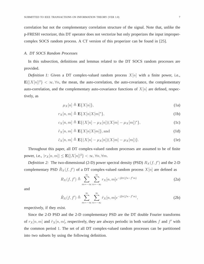
Definition 1: Given a DT complex-valued random processX [n] with a finite power, i.e.,

E|X [n]|2 < ∞, ∀n, the mean, the auto-correlation, the auto-covariance, thecomplementary

auto-correlation, and the complementary auto-covariancefunctions ofX [n] are defined, respec-

tively, as

µX [n] , EX [n], (1a)

rX [n,m] , EX [n]X [m]∗, (1b)

cX [n,m] , E(X [n]− µX [n])(X [m]− µX [m])∗, (1c)

rX [n,m] , EX [n]X [m], and (1d)

cX [n,m] , E(X [n]− µX [n])(X [m]− µX [m]). (1e)

Throughout this paper, all DT complex-valued random processes are assumed to be of finite

power, i.e.,|rX [n,m]| ≤ E|X [n]|2 < ∞, ∀n, ∀m.

Definition 2: The two-dimensional (2-D) power spectral density (PSD)RX(f, f′) and the 2-D

complementary PSDRX(f, f′) of a DT complex-valued random processX [n] are defined as

RX(f, f′) ,

∞∑

m=−∞

∞∑

n=−∞rX [n,m]e−j2π(fn−f ′m) (2a)

and

RX(f, f′) ,

∞∑

m=−∞

∞∑

n=−∞rX [n,m]e−j2π(fn−f ′m), (2b)

respectively, if they exist.

Since the 2-D PSD and the 2-D complementary PSD are the DT double Fourier transforms

of rX [n,m] and rX [n,m], respectively, they are always periodic in both variablesf andf ′ with

the common period1. The set of all DT complex-valued random processes can be partitioned

into two subsets by using the following definition.


Definition 3: [1, Definition 2] A DT complex-valued random processX [n] is proper if its

complementary auto-covariance function vanishes, i.e.,cX [n,m] = 0, ∀n, ∀m, and is improper

otherwise.

Two types of stationarity can be defined as follows by using the second-order moments of a

DT complex-valued random process.

Definition 4: [26, Section II-B] A DT complex-valued random processX [n] is second-order

stationary (SOS) if,∀m, ∀n,

µX [n] = µX [0], (3a)

cX [n,m] = cX [n−m, 0], and (3b)

cX [n,m] = cX [n−m, 0]. (3c)

Definition 5: A DT complex-valued random processX [n] is SOCS with cycle periodM ∈ N

if, ∀n, ∀m,

µX [n] = µX [n+M ], (4a)

cX [n,m] = cX [n+M,m+M ], and (4b)

cX [n,m] = cX [n+M,m+M ]. (4c)

We are mainly interested in the DT SOCS random processes in this paper. Note that a DT

SOS random process can be viewed as a special DT SOCS random process with cycle period1.

Note also that the above definition of a DT SOCS random processis a straightforward extension

of the definition of a CT SOCS random process in [19]. For the ease of comparison with the

results in [19], we use the time indexesm andn in the orders appearing in Definitions 1-5.

In the following lemmas, the implications of the second-order cyclostationarity are provided

in the time and the frequency domains, respectively.

Lemma 1:For a DT SOCS random processX [n] with cycle periodM ∈ N, there exist

(r(k)X [n])M−1

k=0 and (r(k)X [n])M−1k=0 such that

rX [n,m] =M−1∑

k=0

r(k)X [n−m]ej2πkn/M , (5a)

and

rX [n,m] =

M−1∑

k=0

r(k)X [n−m]ej2πkn/M . (5b)


Proof: Sincer′X [n, l] , rX [n, n−l] is periodic inn with periodM and is finite, there exist the

DT Fourier series coefficients(r(k)X [l])M−1k=0 for eachl such thatr′X [n, l] =

∑M−1k=0 r

(k)X [l]ej2πkn/M .

By replacingl with n−m, we obtain (5a). Similarly, we obtain (5b). Therefore, the conclusion

follows.

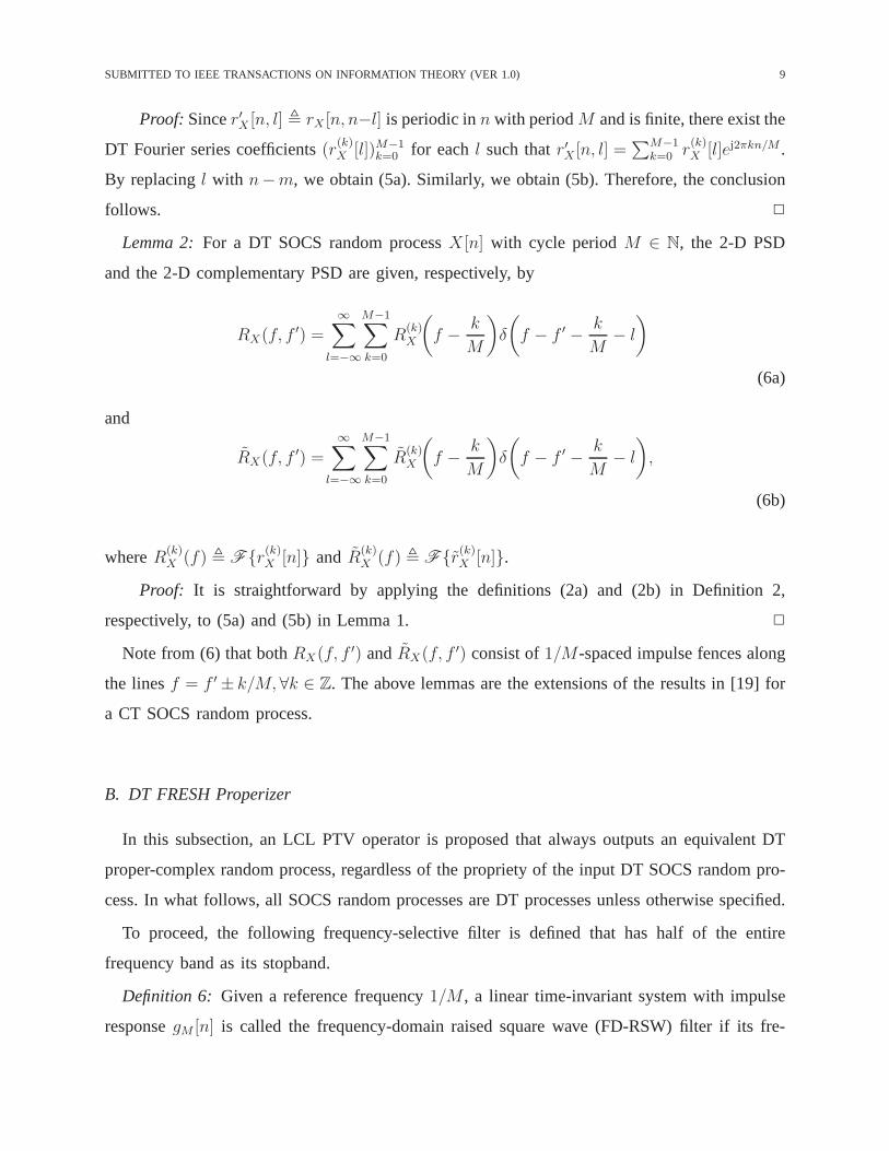
Lemma 2:For a DT SOCS random processX [n] with cycle periodM ∈ N, the 2-D PSD

and the 2-D complementary PSD are given, respectively, by

RX(f, f′) =

∞∑

l=−∞

M−1∑

k=0

R(k)X

(

f − k

M

)

δ

(

f − f ′ − k

M− l

)

(6a)

and

RX(f, f′) =

∞∑

l=−∞

M−1∑

k=0

R(k)X

(

f − k

M

)

δ

(

f − f ′ − k

M− l

)

,

(6b)

whereR(k)X (f) , Fr(k)X [n] and R(k)

X (f) , Fr(k)X [n].

Proof: It is straightforward by applying the definitions (2a) and (2b) in Definition 2,

respectively, to (5a) and (5b) in Lemma 1.

Note from (6) that bothRX(f, f′) andRX(f, f

′) consist of1/M-spaced impulse fences along

the linesf = f ′ ± k/M, ∀k ∈ Z. The above lemmas are the extensions of the results in [19] for

a CT SOCS random process.

B. DT FRESH Properizer

In this subsection, an LCL PTV operator is proposed that always outputs an equivalent DT

proper-complex random process, regardless of the propriety of the input DT SOCS random pro-

cess. In what follows, all SOCS random processes are DT processes unless otherwise specified.

To proceed, the following frequency-selective filter is defined that has half of the entire

frequency band as its stopband.

Definition 6: Given a reference frequency1/M , a linear time-invariant system with impulse

responsegM [n] is called the frequency-domain raised square wave (FD-RSW)filter if its fre-


f

GM(f) , FgM [n]

· · · · · ·

1

− 32M

− 22M

− 12M 0 1

2M2

2M3

2M

Fig. 1. Frequency response of the FD-RSW filter with reference frequency1/M .

quency responseGM(f) = FgM [n] is given by

GM(f) ,

0, for − 12M

≤ f < 0,

1, for 0 ≤ f < 12M

, and

GM

(

f + 1M

)

, elsewhere.

(7)

Fig. 1 shows the frequency response of the FD-RSW filter with reference frequency1/M ,

which alternately passes the frequency components of the input signal in every other interval

of bandwidth1/(2M). Hereafter,GM denotes the support of this FD-RSW filter. By using the

impulse responsegM [n] of the FD-RSW filter with reference frequency1/M , we can define an

LCL PTV filter as follows.

Definition 7: Given a reference frequency1/M and an inputX [n], the DT FRESH properizer

is defined as a single-input single-output LCL PTV system, whose output is given by

Y [n] , X [n] ∗ gM [n] + (X [n]∗ ∗ gM [n]) e−j2πn/(2M). (8)

Fig. 2 shows how the DT FRESH properizer works in the time domain, whereX [n] is the

input, Y [n] is the output, andX1[n] andX2[n] are, respectively, the first and the second terms

on the right side of (8). Note that, unlike the upper branch where X [n] is processed by the

FD-RSW filter to generateX1[n], X [n]∗ is processed in the lower branch by the FD-RSW filter

and multiplied by a complex-exponential functione−j2πn/(2M) to generateX2[n]. Even though

−1/(2M) is chosen as the frequency of the complex-exponential function, any(2k+1)/(2M) for


DT FRESH properizer

X [n] gM [n]

X1[n]

⊕

Y [n]

(·)∗

gM [n] ⊗

e−j2πn/(2M)

X2[n]

Fig. 2. DT FRESH properizer with reference frequency1/M viewed in the time domain.

k ∈ Z can be chosen. The reason why this is so becomes clear once theDT FRESH properization

is viewed in the frequency domain.

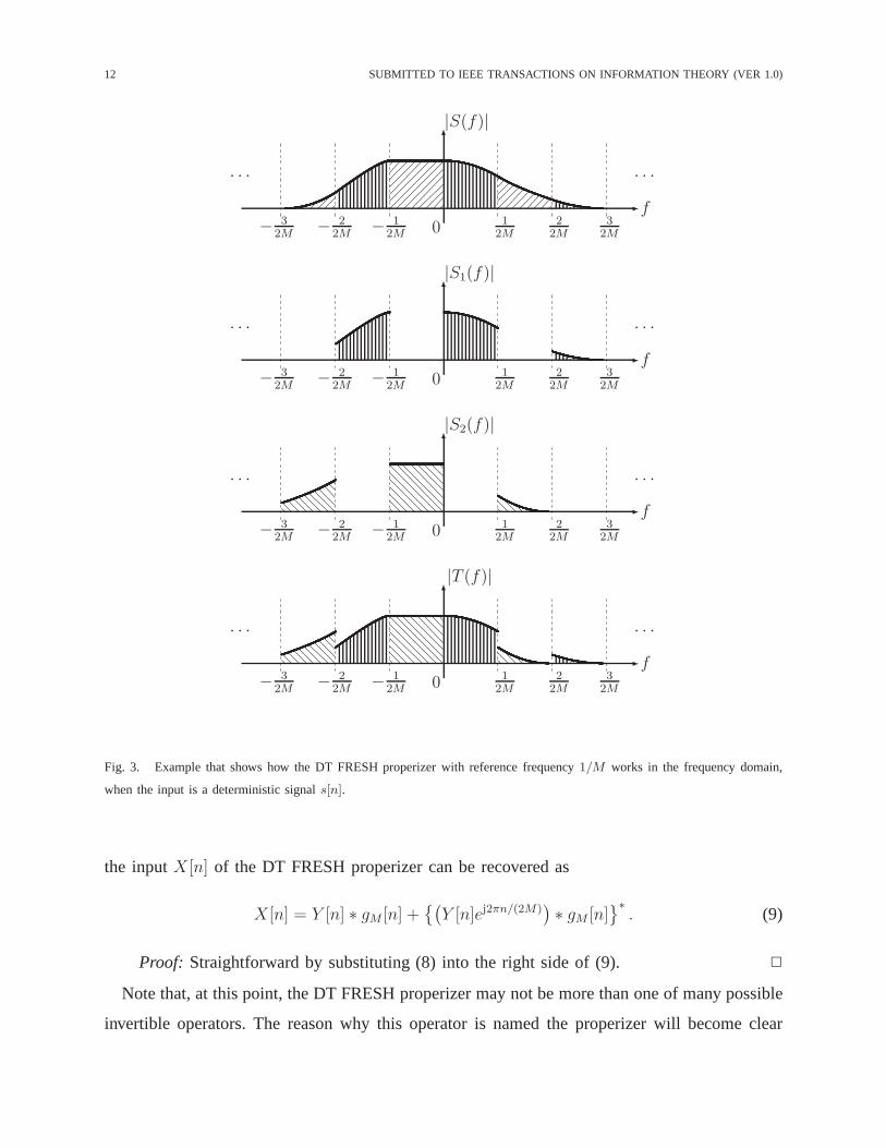
Fig. 3 shows how the DT FRESH properizer works in the frequency domain, especially when

the input is a deterministic signals[n] with the DTFTS(f) , Fs[n], the outputs of the upper

and the lower branches in Fig. 2 are denoted bys1[n] with the DTFTS1(f) , Fs1[n] and

s2[n] with the DTFTS2(f) , Fs2[n], respectively, and the output signal is denoted byt[n]

with the DTFTT (f) , Ft[n]. Note thatS(f) is processed by the FD-RSW filter to generate

the first termS1(f) of the DTFT of the DT FRESH properizer output, whileS(−f)∗ is processed

by the FD-RSW filter and shifted in the frequency domain to generate the second termS2(f).

Thus,S1(f) contains all the frequency components ofs[n] on the supportG of the FD-RSW

filter, while S2(f) contains all the remaining frequency components. Since thesupports ofS1(f)

andS2(f) do not overlap, the DTFT of the outputT (f) of the DT FRESH properizer contains

all the frequency components of the input signalS(f) without any distortion. Note also that,

due to the periodicity of the DTFT with period1, the frequency shift ofS2(f) by any k/M

for k ∈ Z generates the output signal that contains the same information as the input does. The

following lemma makes this invertibility argument more precise.

Lemma 3:From the outputY [n] of the DT FRESH properizer with reference frequency1/M ,


f

|S(f)|

− 32M

− 22M

− 12M 0 1

2M2

2M3

2M

· · ·· · ·

f

|S1(f)|

− 32M

− 22M

− 12M 0 1

2M2

2M3

2M

· · ·· · ·

f

|S2(f)|

− 32M

− 22M

− 12M 0 1

2M2

2M3

2M

· · ·· · ·

f

|T (f)|

− 32M

− 22M

− 12M 0 1

2M2

2M3

2M

· · ·· · ·

Fig. 3. Example that shows how the DT FRESH properizer with reference frequency1/M works in the frequency domain,

when the input is a deterministic signals[n].

the inputX [n] of the DT FRESH properizer can be recovered as

X [n] = Y [n] ∗ gM [n] +(

Y [n]ej2πn/(2M))

∗ gM [n]∗

. (9)

Proof: Straightforward by substituting (8) into the right side of (9).

Note that, at this point, the DT FRESH properizer may not be more than one of many possible

invertible operators. The reason why this operator is namedthe properizer will become clear


once the second-order property of the output is analyzed as follows when its input is a zero-mean

SOCS random process.

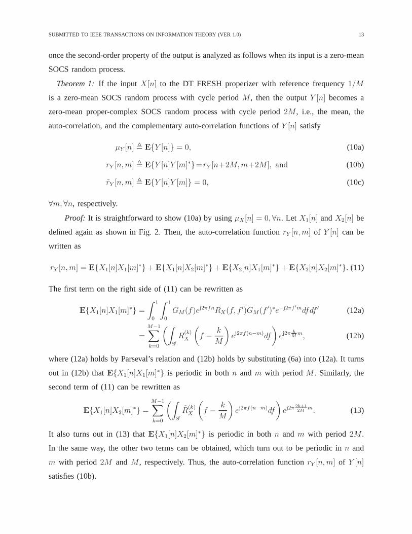
Theorem 1:If the input X [n] to the DT FRESH properizer with reference frequency1/M

is a zero-mean SOCS random process with cycle periodM , then the outputY [n] becomes a

zero-mean proper-complex SOCS random process with cycle period 2M , i.e., the mean, the

auto-correlation, and the complementary auto-correlation functions ofY [n] satisfy

µY [n] , EY [n] = 0, (10a)

rY [n,m] , EY [n]Y [m]∗=rY [n+2M,m+2M ], and (10b)

rY [n,m] , EY [n]Y [m] = 0, (10c)

∀m, ∀n, respectively.

Proof: It is straightforward to show (10a) by usingµX [n] = 0, ∀n. Let X1[n] andX2[n] be

defined again as shown in Fig. 2. Then, the auto-correlation function rY [n,m] of Y [n] can be

written as

rY [n,m] = EX1[n]X1[m]∗+ EX1[n]X2[m]∗+ EX2[n]X1[m]∗+ EX2[n]X2[m]∗. (11)

The first term on the right side of (11) can be rewritten as

EX1[n]X1[m]∗ =

∫ 1

0

∫ 1

0

GM(f)ej2πfnRX(f, f′)GM(f ′)∗e−j2πf ′mdfdf ′ (12a)

=

M−1∑

k=0

(∫

G

R(k)X

(

f − k

M

)

ej2πf(n−m)df

)

ej2πk

Mm, (12b)

where (12a) holds by Parseval’s relation and (12b) holds by substituting (6a) into (12a). It turns

out in (12b) thatEX1[n]X1[m]∗ is periodic in bothn andm with periodM . Similarly, the

second term of (11) can be rewritten as

EX1[n]X2[m]∗ =

M−1∑

k=0

(∫

G

R(k)X

(

f − k

M

)

ej2πf(n−m)df

)

ej2π2k+1

2Mm. (13)

It also turns out in (13) thatEX1[n]X2[m]∗ is periodic in bothn andm with period 2M .

In the same way, the other two terms can be obtained, which turn out to be periodic inn and

m with period 2M andM , respectively. Thus, the auto-correlation functionrY [n,m] of Y [n]

satisfies (10b).


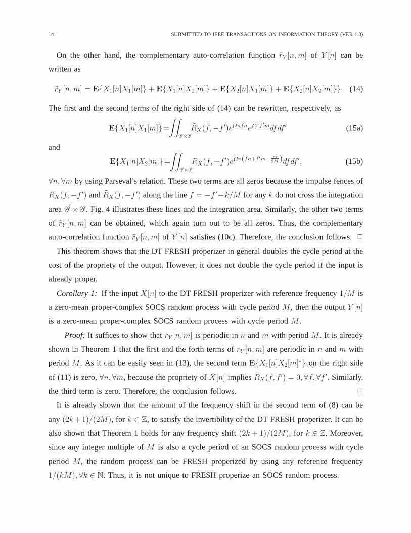
On the other hand, the complementary auto-correlation function rY [n,m] of Y [n] can be

written as

rY [n,m] = EX1[n]X1[m]+ EX1[n]X2[m] + EX2[n]X1[m] + EX2[n]X2[m]. (14)

The first and the second terms of the right side of (14) can be rewritten, respectively, as

EX1[n]X1[m]=∫∫

G×G

RX(f,−f ′)ej2πfnej2πf′mdfdf ′ (15a)

and

EX1[n]X2[m]=∫∫

G×G

RX(f,−f ′)ej2π(fn+f ′m− m

2M )dfdf ′, (15b)

∀n, ∀m by using Parseval’s relation. These two terms are all zeros because the impulse fences of

RX(f,−f ′) andRX(f,−f ′) along the linef = −f ′−k/M for anyk do not cross the integration

areaG ×G . Fig. 4 illustrates these lines and the integration area. Similarly, the other two terms

of rY [n,m] can be obtained, which again turn out to be all zeros. Thus, the complementary

auto-correlation functionrY [n,m] of Y [n] satisfies (10c). Therefore, the conclusion follows.

This theorem shows that the DT FRESH properizer in general doubles the cycle period at the

cost of the propriety of the output. However, it does not double the cycle period if the input is

already proper.

Corollary 1: If the inputX [n] to the DT FRESH properizer with reference frequency1/M is

a zero-mean proper-complex SOCS random process with cycle periodM , then the outputY [n]

is a zero-mean proper-complex SOCS random process with cycle periodM .

Proof: It suffices to show thatrY [n,m] is periodic inn andm with periodM . It is already

shown in Theorem 1 that the first and the forth terms ofrY [n,m] are periodic inn andm with

periodM . As it can be easily seen in (13), the second termEX1[n]X2[m]∗ on the right side

of (11) is zero,∀n, ∀m, because the propriety ofX [n] implies RX(f, f′) = 0, ∀f, ∀f ′. Similarly,

the third term is zero. Therefore, the conclusion follows.

It is already shown that the amount of the frequency shift in the second term of (8) can be

any (2k+1)/(2M), for k ∈ Z, to satisfy the invertibility of the DT FRESH properizer. Itcan be

also shown that Theorem 1 holds for any frequency shift(2k+ 1)/(2M), for k ∈ Z. Moreover,

since any integer multiple ofM is also a cycle period of an SOCS random process with cycle

period M , the random process can be FRESH properized by using any reference frequency

1/(kM), ∀k ∈ N. Thus, it is not unique to FRESH properize an SOCS random process.


f

f ′

12M

32M

− 12M

− 32M

12M

32M

− 12M

− 32M

. . . . . .

...

...

Fig. 4. Solid lines represent the impulse fences ofRX(f,−f ′), RX(−f, f ′), RX(f,−f ′), or RX(−f, f ′). Shaded area

represents the integration areaG × G .

III. A SYMPTOTIC FRESH PROPERIZER

In this section, the block processing of an SOCS random process is considered. Motivated

by how the DT FRESH properizer works in the frequency domain,an LCL block operator is

proposed that converts a finite number of consecutive samples of an SOCS random process to an

equivalent random vector. Unlike the DT FRESH properizer proposed in the previous section,

this invertible operator does not directly make the complementary covariance matrix of the output

vector vanish. Instead, it is shown that the LCL operator makes the complementary covariance

matrix of the output vector approach all-zero matrix as the number of samples tends to infinity.

This is why it is named the asymptotic FRESH properizer.


A. Asymptotic FRESH Properizer and Its Inverse Operator

Let x be the length-MN vector obtained by taking theMN consecutive samples of a DT

signal, where and in what follows it is assumed thatN is a positive even number. Motivated

by the DT FRESH properizer, we introduce in this subsection an LCL block operator and its

inverse.

To proceed, some definitions are provided.

Definition 8: The centered DFT matrixWMN is defined as an(MN)-by-(MN) matrix whose

(m,n)th entry, form,n ∈ 1, · · · ,MN, is given by

[WMN ]m,n ,1√MN

e−j2π(m−cMN )(n−cMN )/(MN), (16)

wherecMN , (MN + 1)/2.

It is well known that the matrix-vector multiplication witha centered DFT matrix can be

implemented with low computational complexity [27], as themultiplication with an ordinary

DFT matrix is efficiently implemented by using the fast Fourier transform algorithm.

Definition 9: GivenM and an even numberN , the(MN)-by-(MN) matrixGM,N is defined

as

GM,N , IM ⊗

ON/2 ON/2

ON/2 IN/2

. (17)

Similar to the FD-RSW pulse, the matrixGM,N will be called the raised square wave (RSW)

matrix because, when pre-multiplied to a column vector or a matrix, it turns the((m−1)N+n)th

row, for m = 1, · · · ,M andn = 1, · · · , N/2, into all zeros, i.e., it alternately nulls every other

band ofN/2 consecutive rows.

Definition 10: GivenM and an even numberN , the(MN)-by-(MN) matrixSM,N is defined

as

SM,N ,

OMN−N/2,N/2 IMN−N/2

IN/2 ON/2,MN−N/2

. (18)

Note that the matrixSM,N , when pre-multiplied to a column vector or a matrix, circularly

shifts the rows byN/2, which corresponds to multiplyinge−j2πn/(2M) in the second term of the


right side of (8). Now, we are ready to introduce an LCL operator that is the block-processing

counterpart to the DT FRESH propertizer.

Definition 11: GivenM and an even numberN , the LCL operatorf with inputx and output

y = f (x), both of lengthMN , is called the asymptotic FRESH properizer if

f (x) , WHMN

(

GM,NWMNx+ SM,NGM,NWMNx∗). (19)

Note that the inputx is pre-multiplied by the centered DFT matrixWMN and the RSW matrix

GM,N , while the complex conjugatex∗ is multiplied additionally by the circular shift matrix

SM,N to generate the frequency-domain outputWMNy.

Fig. 5 showsWMNx, GM,NWMNx, andSM,N GM,NWMNx∗, when thelth entry of the

WMNx is denoted byx′l. Note that, similar to the DT FRESH properization illustrated in Fig. 3,

the locations of all possible non-zero rows ofGM,NWMNx and SM,NGM,NWMNx∗ do not

overlap, which makesWMNy contain all the entries ofWMNx without any distortion. Note

also that the amount of the circular shift ofSM,NGM,NWMNx∗ by anykN for k ∈ Z generates

the signal that contains the same information asSM,NGM,NWMNx∗ does. The following lemma

makes this invertibility argument more precise.

Lemma 4:From the outputy of the asymptotic FRESH properizer with parametersM and

N , the inputx of the asymptotic FRESH properizer can be recovered as

x = WHMN

(

GM,NWMNy + PMNGM,NSTM,NW

∗MNy

∗) (20a)

, f−1(y) (20b)

Proof: By substituting (19) into the right side of (20a), we haveWHMNG

2M,NWMNx +

WHMNGM,N SM,NGM,NWMNx

∗ +WHMNPMNGM,NS

TM,NGM,N W ∗

MNx∗ +WH

MNPMNGM,N ·ST

M,NSM,NGM,NW∗MNx. The second and the third terms vanish sinceGM,NSM,NGM,N = OMN

andGM,NSTM,NGM,N =OMN , respectively. Thus, the right side of (20a) becomesWH

MN(G2M,N+

PMNG2M,NPMN)WMNx. Moreover, it can be easily shown thatG2

M,N = GM,N and GM,N

+PMNGM,NPMN = IMN , becausePMN = PM ⊗ PN by the properties of the Kronecker

product. Therefore, the conclusion follows.

Note that, at this point, the asymptotic FRESH properizer may not be more than one of many

possible invertible operators. The reason why this operator is named the asymptotic properizer

will become clear once the second-order property of the output is analyzed in the next subsection

when its input is a finite number of consecutive samples of a zero-mean SOCS random process.


(a) WMNx

x′

1

...

x′

N/2

x′

N/2+1

...

x′

N

...

x′

MN−N+1

...

x′

MN−N/2

x′

MN−N/2+1

...

x′

MN

(b) GM,NWMNx

0

...

0

x′

N/2+1

...

x′

N

...

0

...

0

x′

MN−N/2+1

...

x′

MN

(c) SM,NGM,NWMNx∗

x′∗

MN−N/2

...

x′∗

MN−N+1

0

...

0

...

x′∗

N/2

...

x′∗

1

0

...

0

Fig. 5. Illustration that shows how the asymptotic FRESH properizer works in the frequency domain.

B. Second-Order Properties of Output of Asymptotic FRESH Properizer

Let x be the length-2MN augmented vector defined as

x ,

x

x∗

, (21)


where and in what follows it is assumed thatx consists of a finite number of consecutive

samples of azero-meanSOCS random processX [n] with cycle periodM ∈ N. Then, the output

y = f (x) in (19) of the asymptotic FRESH properizer can be rewritten as

y = WHMNGM,NWMN x (22a)

, WHMN y, (22b)

where the(MN)-by-(2MN) matrix GM,N and the(2MN)-by-(2MN) matrix WMN are given

by

GM,N ,

[

GM,N SM,NGM,N

]

and (23a)

WMN ,

WMN OMN

OMN WMN

, (23b)

respectively, andy is the centered DFT ofy. Thus, the covariance matrixRy , EyyH and

the complementary covariance matrixRy , EyyT of y are given by

Ry = WHMNGM,NWMNRxW

HMNG

HM,NWMN (24a)

and

Ry = WHMNGM,NWMNRxW

TMNG

TM,NW

∗MN , (24b)

respectively, whereRx , ExxH andRx , ExxT denote the covariance and the comple-

mentary covariance matrices of the augmented vectorx, respectively.

Throughout this paper, we call

Ry , EyyH = WMNRyWHMN (25a)

and

Ry , EyyT = WMNRyWTMN (25b)

the frequency-domain covariance and the frequency-domaincomplementary covariance matrices,

respectively.

To analyze the asymptotic second-order properties ofy, we briefly review definitions and

related lemmas for asymptotic equivalence between two sequences of matrices.


Definition 12: [23] Let (Ak)k and (Bk)k be two sequences ofNk-by-Nk matrices with

Nk → ∞ as k → ∞. Then, (Ak)k and (Bk)k are asymptotically equivalent and denoted by

Ak ∼ Bk if 1) the strong norms ofAk andBk are uniformly bounded, i.e., there exists a constant

c such that‖Ak‖, ‖Bk‖ ≤ c < ∞, ∀k, and 2) the weak norm ofAk−Bk vanishes asymptotically,

i.e., limk→∞ |Ak − Bk| = 0, where the strong norm‖A‖ and the weak norm|A| of an Nk-

by-Nk matrix A are defined as‖A‖ , maxx6=0

√

xHAHAx/xHx and |A| ,√

tr(AAH)/Nk,

respectively.

Lemma 5: If two sequences(Ak)k and(Bk)k of Nk-by-Nk matrices are asymptotically equiv-

alent and if the strong norms ofNk-by-Nk matricesCk andDk are uniformly bounded, then

CkAkDk ∼ CkBkDk.

Proof: SinceCk ∼ Ck and Dk ∼ Dk, it is straightforward to show the conclusion by

applying [23, Theorem 1-(3)] twice.

Lemma 6: If Ak ∼ Bk andCk ∼ Dk, then (Ak +Ck) ∼ (Bk +Dk).

Proof: By applying the triangle inequality, it is straightforwardto show that the strong norms

of Ak+Ck andBk+Dk are uniformly bounded and that the weak norm ofAk+Ck−Bk−Dk

vanishes asymptotically. Therefore, the conclusion follows.

For brevity, in what follows, two square matricesAk andBk of the same size will be said

to be asymptotically equivalent ifAk ∼ Bk. Now, we introduce our definition of asymptotic

propriety.

Definition 13: A sequence(yk)k of length-Nk complex-valued random vectors is asymptoti-

cally proper if the complementary covariance matrix ofyk is asymptotically equivalent to the

Nk-by-Nk all-zero matrix.

For brevity, a random vectoryk will be said to be asymptotically proper if the sequence(yk)k

is asymptotically proper. Before showing that the outputy of the asymptotic FRESH properizer

is asymptotically proper, the second-order properties of the augmented vectorx are examined

as follows.

Proposition 1: If the random vectorx is obtained by taking theMN consecutive samples

from a zero-mean SOCS random process with cycle periodM , then the covariance matrixRx


and the complementary covariance matrixRx of the augmented vectorx defined in (21) satisfy

WMNRxWHMN ∼ Ω (26a)

and

WMNRxWTMN ∼ Ω, (26b)

respectively, where the(2MN)-by-(2MN) matricesΩ andΩ are given by

Ω , (WMNRxWHMN)⊙ (12M ⊗ IN) (27a)

and

Ω , (WMNRxWTMN)⊙ (12M ⊗PN ), (27b)

respectively.

Proof: By definition, the left sides of (26a) and (26b) can be rewritten, respectively, as

WMNRxWHMN =

WMNRxWHMN WMNRxW

HMN

WMNR∗xW

HMN WMNR

∗xW

HMN

(28a)

and

WMNRxWTMN =

WMNRxWTMN WMNRxW

TMN

WMNR∗xW

TMN WMNR

∗xW

TMN

.

(28b)

Since bothRx andRx are (MN)-by-(MN) block Toeplitz matrices with block sizeM-by-M ,

each submatrix on the right side of (28a) is asymptotically equivalent to the Hadamard product

of (1M ⊗ IN) and the submatrix itself as shown in [24, Proposition 1]. Thus, by using the fact

thatA ∼ B if each submatrix ofA is asymptotically equivalent to the corresponding submatrix

of B [24, Lemma 5], we obtain (26a). Similar to (26a), it can be shown by using the property

W TMN = WH

MNPMN of the centered DFT matrix that each submatrix on the right side of (28b)

is asymptotically equivalent to Hadamard product of(1M ⊗PN) and the submatrix itself. Thus,

we obtain (26b). Therefore, the conclusion follows.


(a) (b)

(c) (d)

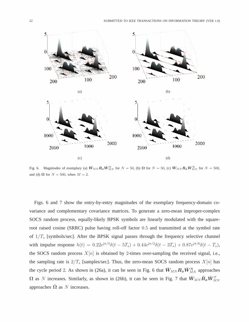
Fig. 6. Magnitudes of exemplary (a)WMNRxWHMN for N = 50, (b) Ω for N = 50, (c) WMNRxW

HMN for N = 500,

and (d)Ω for N = 500, whenM = 2.

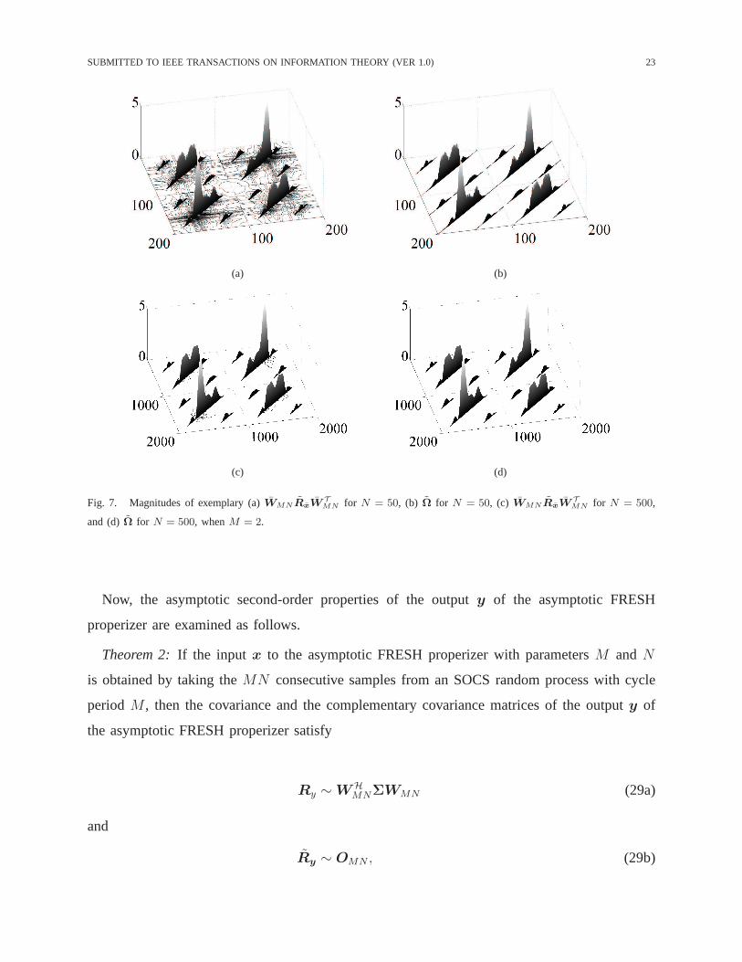
Figs. 6 and 7 show the entry-by-entry magnitudes of the exemplary frequency-domain co-

variance and complementary covariance matrices. To generate a zero-mean improper-complex

SOCS random process, equally-likely BPSK symbols are linearly modulated with the square-

root raised cosine (SRRC) pulse having roll-off factor0.5 and transmitted at the symbol rate

of 1/Ts [symbols/sec]. After the BPSK signal passes through the frequency selective channel

with impulse responseh(t) = 0.22ejπ/3δ(t − 5Ts) + 0.44ejπ/2δ(t − 3Ts) + 0.87ejπ/6δ(t − Ts),

the SOCS random processX [n] is obtained by2-times over-sampling the received signal, i.e.,

the sampling rate is2/Ts [samples/sec]. Thus, the zero-mean SOCS random processX [n] has

the cycle period2. As shown in (26a), it can be seen in Fig. 6 thatWMNRxWHMN approaches

Ω asN increases. Similarly, as shown in (26b), it can be seen in Fig. 7 thatWMNRxWTMN

approachesΩ asN increases.


(a) (b)

(c) (d)

Fig. 7. Magnitudes of exemplary (a)WMNRxWTMN for N = 50, (b) Ω for N = 50, (c) WMNRxW

TMN for N = 500,

and (d)Ω for N = 500, whenM = 2.

Now, the asymptotic second-order properties of the outputy of the asymptotic FRESH

properizer are examined as follows.

Theorem 2:If the input x to the asymptotic FRESH properizer with parametersM andN

is obtained by taking theMN consecutive samples from an SOCS random process with cycle

periodM , then the covariance and the complementary covariance matrices of the outputy of

the asymptotic FRESH properizer satisfy

Ry ∼ WHMNΣWMN (29a)

and

Ry ∼ OMN , (29b)


where an(MN)-by-(MN) matrix Σ is given by

Σ , GM,NΩGHM,N (30a)

= Ry ⊙ (12M ⊗ IN/2). (30b)

Proof: By applying Lemmas 5 and 6 to (24a) and (26a), we obtainRy ∼ GM,NΩGHM,N .

SinceGM,NΩGHM,N can be rewritten as(GM,NWMNRxW

HMNG

HM,N)⊙(GM,N (12M⊗IN )G

HM,N)

by the definition (27a), we obtainRy ∼ Σ from GM,N(12M⊗IN)GHM,N=12M⊗IN/2. Similarly,

Ry ∼ (GM,NWMNRxWTMNG

TM,N ) ⊙ (GM,N(12M ⊗ PN )G

TM,N) by (24b), (26b), and (27b).

Thus, we obtainRy ∼ OMN from GM,N(12M ⊗PN )GTM,N = OMN . Therefore, the conclusion

follows by Lemma 5.

By Definition 13 and the above theorem, the outputy of the asymptotic FRESH properizer is

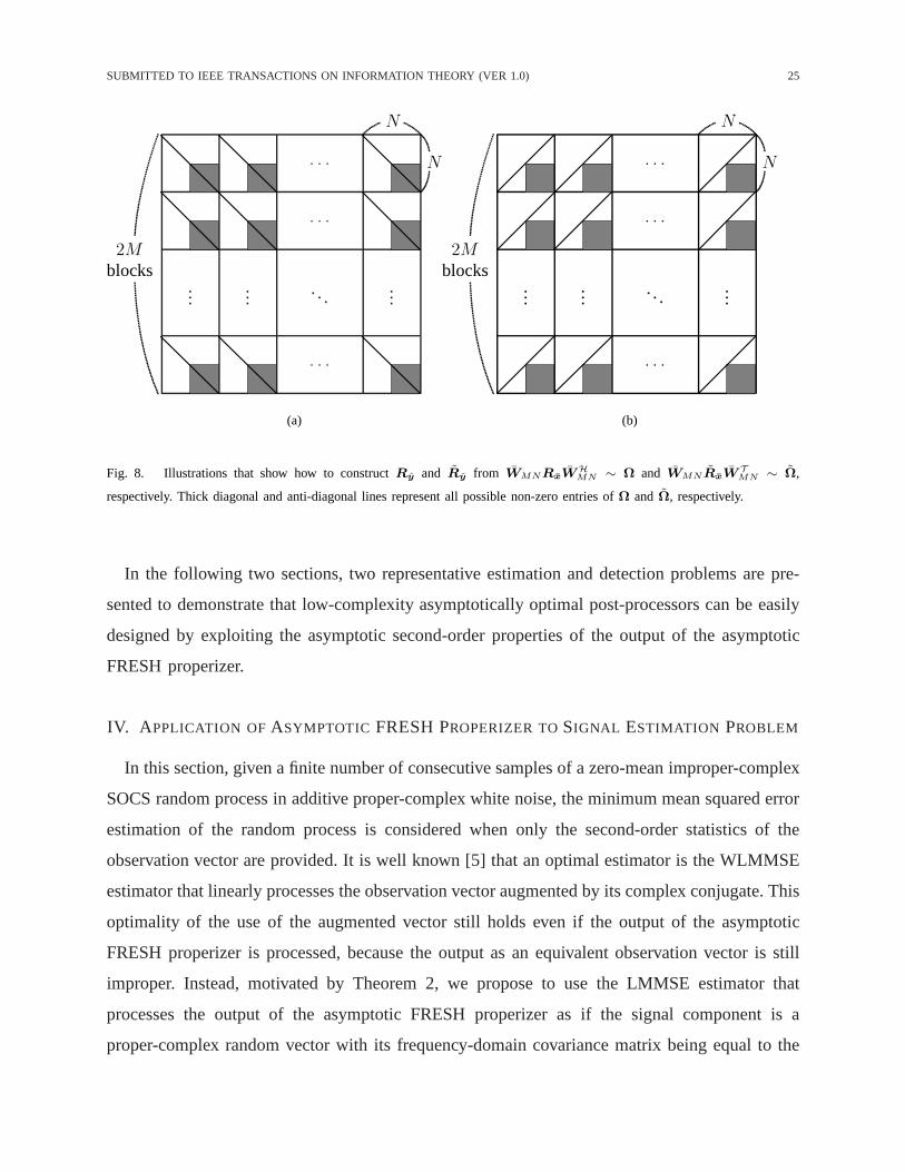
indeed asymptotically proper. Fig. 8-(a) illustrates how the frequency-domain covariance matrix

Ry of the outputy of the asymptotic FRESH properizer is constructed fromWMNRxWHMN .

The thick diagonal lines in each block of sizeN-by-N represent all possible non-zero entries

of Ω that is asymptotically equivalent toWMNRxWHMN . Then, Ry that is asymptotically

equivalent toΣ is obtained by collecting the shaded sub-blocks of size(N/2)-by-(N/2). Fig. 8-

(b) illustrates how the frequency-domain complementary covariance matrixRy of the output

y of the asymptotic FRESH properizer is constructed fromWMNRxWTMN . The thick anti-

diagonal lines in each block of sizeN-by-N represent all possible non-zero entries ofΩ that

is asymptotically equivalent toWMNRxWTMN . Then,Ry that is asymptotically equivalent to

OMN is obtained by collecting the shaded sub-blocks of size(N/2)-by-(N/2).

It is already shown that the amount of the circular shift ofGM,NWMNx∗ in (17) can be

anyN(2k + 1)/2, for k ∈ Z, to satisfy the invertibility of the asymptotic FRESH properizer. It

can be also shown that Theorem 2 holds for every circular shift by N(2k + 1)/2, for k ∈ Z.

Moreover, sinceRx andRx that are(MN)-by-(MN) block Toeplitz matrices with block size

M-by-M can be viewed as block Toeplitz matrices with block size(lM)-by-(lM), ∀l ∈ N, the

sampled vectorx can be asymptotically properized by using any parameterslM andN/l, for

all l ∈ N such thatN/l is even. Thus, similar to the DT FRESH properizer, it is not unique to

asymptotically properize a finite number of consecutive samples of a zero-mean SOCS random

process with cycle periodM .


......

...

. . .

. . .

. . .

. . .

N

N

2Mblocks

(a)

......

...

. . .

. . .

. . .

. . .

N

N

2Mblocks

(b)

Fig. 8. Illustrations that show how to constructRy and Ry from WMNRxWHMN ∼ Ω and WMNRxW

TMN ∼ Ω,

respectively. Thick diagonal and anti-diagonal lines represent all possible non-zero entries ofΩ and Ω, respectively.

In the following two sections, two representative estimation and detection problems are pre-

sented to demonstrate that low-complexity asymptoticallyoptimal post-processors can be easily

designed by exploiting the asymptotic second-order properties of the output of the asymptotic

FRESH properizer.

IV. A PPLICATION OFASYMPTOTIC FRESH PROPERIZER TOSIGNAL ESTIMATION PROBLEM

In this section, given a finite number of consecutive samplesof a zero-mean improper-complex

SOCS random process in additive proper-complex white noise, the minimum mean squared error

estimation of the random process is considered when only thesecond-order statistics of the

observation vector are provided. It is well known [5] that anoptimal estimator is the WLMMSE

estimator that linearly processes the observation vector augmented by its complex conjugate. This

optimality of the use of the augmented vector still holds even if the output of the asymptotic

FRESH properizer is processed, because the output as an equivalent observation vector is still

improper. Instead, motivated by Theorem 2, we propose to usethe LMMSE estimator that

processes the output of the asymptotic FRESH properizer as if the signal component is a

proper-complex random vector with its frequency-domain covariance matrix being equal to the


masked version of the exact frequency-domain covariance matrix. It turns out that this suboptimal

linear estimator is asymptotically optimal in the sense that the difference of its average MSE

performance from that of the WLMMSE estimator having highercomputational complexity

converges to zero as the number of samples tends to infinity.

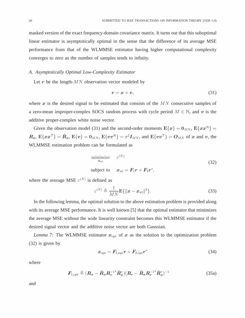
A. Asymptotically Optimal Low-Complexity Estimator

Let r be the length-MN observation vector modeled by

r = x+ v, (31)

wherex is the desired signal to be estimated that consists of theMN consecutive samples of

a zero-mean improper-complex SOCS random process with cycle periodM ∈ N, andv is the

additive proper-complex white noise vector.

Given the observation model (31) and the second-order moments Ex = 0MN , ExxH =

Rx, ExxT = Rx, Ev = 0MN , EvvH = σ2IMN , andEvvT = OMN of x andv, the

WLMMSE estimation problem can be formulated as

minimizexwl

ε(N)

subject to xwl = F1r + F2r∗,

(32)

where the average MSEε(N) is defined as

ε(N) ,1

MNE‖x− xwl‖2. (33)

In the following lemma, the optimal solution to the above estimation problem is provided along

with its average MSE performance. It is well known [5] that the optimal estimator that minimizes

the average MSE without the wide linearity constraint becomes this WLMMSE estimator if the

desired signal vector and the additive noise vector are bothGaussian.

Lemma 7:The WLMMSE estimatorxopt of x as the solution to the optimization problem

(32) is given by

xopt = F1,optr + F2,optr∗ (34)

where

F1,opt , (Rx − RxR−1r

∗R∗

x)(Rr − RxR

−1r

∗R∗

x)−1 (35a)

and


F2,opt , (Rx − R∗xR−1

rRx)(R

∗r− R∗

xR−1

rRx)

−1. (35b)

with Rr , ErrH = σ2IMN+Rx. Moreover, the average MSEε(N)opt , E‖x−xopt‖2/(MN)

is given by

ε(N)opt =

1

MNtr(Rx − F1,optRx − F2,optR

∗x). (36)

Proof: See [5, Section 5.4] and the references therein.

The WLMMSE estimator in (34) requires the computation of twomatricesF1,opt andF2,opt

to be pre-multiplied tor and r∗, respectively. As it can be seen from (35a) and (35b), the

major burden in computing these matrices comes from the multiplications and the inversions of

(MN)-by-(MN) matrices. It can be shown that the matrix multiplications incomputingF1,opt

and F2,opt requireO(M3N3) complex-valued scalar multiplications because the matrixR−1r

does not have any structure to be exploited in matrix-matrixmultiplications even thoughRr

is block Toeplitz. By the same reason, the matrix inversion(Rr − RxR−1r

∗R∗

x) in (35a) and

(35b) requiresO(M3N3) complex-valued scalar multiplications. Thus, the overallcomputational

complexity of the WLMMSE estimator isO(M3N3).

An alternative observation model that is equivalent to the original one in (31) can be obtained

by applying the asymptotic FRESH properization tor as

s = y +w, (37)

wheres = f (r), y = f (x), andw = f (v). Since the equivalent observation vectors is not

proper in general, the linear processing ofs ands∗ is still needed for the second-order optimal

estimation ofx. Instead, we propose to use a suboptimal linear estimator asfollows, which is

a function only ofs.

Definition 14: The proposed estimatexp of x is defined by

xp = f−1(Fps), (38)

whereFp is given by

Fp , WHMNΣ(σ2IMN +Σ)−1WMN . (39)

Note from (38) and (39) thatΣ(σ2IMN+Σ)−1WMNs is the estimate ofWMNy = WMNf (x)

and, consequently, thatFps is the estimate ofy = f (x). Let yp , Fps. Then, the estimatexp

of x = f−1(y) is obtained as (38) by applying the inverse operationf−1 to yp.


It can be immediately seen thatFp is chosen to makeyp the LMMSE estimate ofy when the

covariance and the complementary covariance matrices ofy are set equal toWHMNΣWMN and

OMN appearing in (29a) and (29b), respectively. This idea of using the asymptotically equivalent

matrices is motivated by Theorem 2, which naturally leads tothe asymptotic optimality of the

proposed estimator as shown in what follows.

First, the invariance of the Euclidean norm under the asymptotic FRESH properization is

shown.

Lemma 8:The inputx and the outputy = f (x) of the asymptotic FRESH properizer have

the same Euclidean norm, i.e.,‖x‖ = ‖y‖.

Proof: Since the centered DFT matrixWMN is unitary, we have‖x‖ = ‖WMNx‖. Let

yl and y′l denote thelth entries ofy andWMNx, respectively. Then, we have‖WMNx‖2 =∑MN

l=1 |y′l|2 =∑MN

l=1 |yl|2 = ‖y‖2 by Definition 11 off (x) in (19), which is illustrated in Fig. 5.

Therefore, the conclusion follows.

Second, the average MSE of the proposed estimator is derived.

Lemma 9:The average MSEε(N)p , E‖x−xp‖2/(MN) of the proposed estimator is given

by

ε(N)p =

1

MNtrΣ−Σ(σ2IMN +Σ)−1

Σ. (40)

Proof: The linearity of the asymptotic FRESH properizer leads toy−yp = f (x−xp). Then,

by Lemma 8, the average MSE performance can be written asε(N)p = E‖y − yp‖2/(MN).

SinceWMN is unitary andyp = Fps, it can be shown that we have

ε(N)p =

1

MNtrRy − 2Σ(σ2IMN +Σ)−1Ry

+Σ(σ2IMN +Σ)−1(σ2IMN +Ry)(σ2IMN +Σ)−1

Σ. (41)

It can be also shown that ifA , A ⊙ (12M ⊗ IN/2) and B , B ⊙ (12M ⊗ IN/2) for (MN)-

by-(MN) matricesA andB then tr(A) = tr(A) and tr(AB) = tr(AB). Thus, the right side

of (41) is invariant under replacingRy with Σ = Ry ⊙ (12M ⊗ IN/2) in (30b). Therefore, (41)

can be simplified to (40).

Now, the asymptotic optimality of the proposed estimator isprovided.

Theorem 3:The average MSE of the proposed estimator approaches that ofthe WLMMSE


estimator as the number of samples tends to infinity in the sense that

limN→∞

(

ε(N)p − ε

(N)opt

)

= 0. (42)

Proof: It is shown in [5, Section 5.4] that the average MSEε(N)opt in (36) of the WLMMSE

estimator can be simplified as

ε(N)opt =

1

2MNtrRx −Rx(σ

2I2MN +Rx)−1Rx. (43)

Now, we defineΩ , WHMNΩWMN and introduce

ε(N)opt ,

1

2MNtrΩ− Ω(σ2I2MN + Ω)−1

Ω (44a)

=1

2MNtrΩ−Ω(σ2I2MN +Ω)−1

Ω, (44b)

which is obtained by replacingRx in (43) with Ω and by using the fact thatWMN is unitary.

Note thatWMNRxWHMN ∼ Ω as shown in (26a). This introduction ofε(N)

opt is motivated by

the result in [24, Theorem 1], where a suboptimal estimator is proposed for the estimation of a

proper-complex cyclostationary random signal and its average MSE is shown to approach that

of the LMMSE estimator as the number of samples tends to infinity. SinceRx is a covariance

matrix, it is positive semidefinite, which implies that all the eigenvalues of(σ2I2MN +Rx)−1

in (43) are upper bounded by1/σ2. Note thatΩ and Ω are also positive semidefinite because

(12M ⊗IN/2) in (27a) is positive semidefinite. Similarly, all the eigenvalues of(σ2I2MN + Ω)−1

in (44a) are also upper bounded by1/σ2. Thus, the strong norms‖(σ2I2MN + Rx)−1‖ and

‖(σ2I2MN + Ω)−1‖ are uniformly upper bounded by1/σ2 for any matrix size. Recall that if

Ak ∼ Bk and ‖A−1k ‖, ‖B−1

k ‖ ≤ c < ∞, ∀k, for a positive constantc, then A−1k ∼ B−1

k

[23, Theorem 1-(4)]. Thus, we have(σ2I2MN + Rx)−1 ∼ (σ2I2MN + Ω)−1. Recall also that

if two sequences(Ak)k and (Bk)k of Nk-by-Nk matrices are asymptotically equivalent then

limk→∞ tr(Ak−Bk)/Nk = 0 [23, Corollary 1]. Thus, combined with Lemmas 5 and 6, we have

limN→∞(ε(N)opt − ε

(N)opt ) = 0. Therefore, in order to show (42), it now suffices to showε

(N)opt = ε

(N)p .

Let E2M,N be the(2MN)-by-(2MN) matrix that permutes the rows of the post-multiplied

matrix in such a way that the(N(m − 1) + n)th row of the post-multiplied matrix becomes

the (2M(n − 1) +m)th row for m = 1, 2, · · · , 2M andn = 1, 2, · · · , N , i.e., the rows having

indexes(N(m− 1) + n), for m = 1, 2, · · · , 2M, are grouped for eachn. Then,E2M,NΩET2M,N

is a (2MN)-by-(2MN) block diagonal matrix with block size(2M)-by-(2M), becauseΩ is


a (2MN)-by-(2MN) block matrix with diagonal blocks of block sizeN-by-N . Similarly, the

(MN)-by-(MN) matrixE2M,N/2 is defined. LetE1 andE2 be the(MN)-by-(MN) matrix that

are defined asE1 , PMN(IN/2 ⊗ E2M)E2M,N/2 andE2 , (IN/2 ⊗ E2M)E2M,N/2, respectively,

where the(2M)-by-(2M) matrix E2M permutes the rows of the post-multiplied matrix in such

a way that the(2m)th row becomes themth row and that the(2m − 1)th row becomes the

(M +m)th row for m = 1, 2, · · · ,M . Then, the definitionΣ , GM,NΩGHM,N in (30a) leads to

E2M,NΩET2M,N =

E1Σ∗ET

1 OMN

OMN E2ΣET2

. (45)

SinceE2M,N , E1, andE2 are all permutation matrices,ε(N)opt in (44a) can be rewritten asε(N)

opt =

trΣ∗−Σ∗(σ2I2MN+Σ

∗)−1Σ

∗+Σ−Σ(σ2I2MN+Σ)−1Σ/(2MN), which leads toε(N)

opt = ε(N)p

becauseΣ is Hermitian symmetric. Therefore, the conclusion follows.

The proposed estimator requires the pre-processing ofr to obtains, the computation and the

multiplication ofFp, and the inverse operation onyp to obtainxp. As it can be seen from (19) and

(20), the major burden in the asymptotic FRESH properization and its inverse operation comes

from the multiplications of the(MN)-by-(MN) centered DFT matrix. This can be efficiently

implemented with onlyO(MN log(MN)) complex-valued scalar multiplications by using, e.g.,

the fast algorithm in [27]. As it can be seen from (39), the major burden in computingFp comes

from the inversion of(σ2I2MN +Σ). The inversion of an(MN)-by-(MN) block matrix with

diagonal blocks of sizeN-by-N requiresO(M3N) complex-valued scalar multiplications [24].

Thus, this inversion of(σ2I2MN +Σ) has the same orderO(M3N) of computational complexity

becauseΣ is an (MN)-by-(MN) block matrix with diagonal blocks of size(N/2)-by-(N/2).

Since we consider the block processing whereM is a fixed small number andN is much larger

thanM , the overall complexities of the WLMMSE and the proposed estimators as functions only

of N can be rewritten now asO(N3) andO(N logN), respectively. Thus, the computational

complexity of the proposed estimator is much lower than thatof the WLMMSE estimator.

Though not major, an additional complexity reduction comesfrom the fact that the proposed

estimator is linear that requires the computation and multiplication of one matrixFp instead of

two matricesF1,opt andF2,opt, all with MN(≫ 1) columns.


0 100 200 300

102

104

106

108

1010

1012

N

num

ber

ofco

mple

x-v

alu

edm

ult

iplica

tions

O(N3)WLMMSEO(N logN)proposed

M = 2

M = 1

M = 4

Fig. 9. Computational complexities of the WLMMSE and the proposed estimators.

B. Numerical Results

In this subsection, numerical results are provided that show the computational efficiency and

the asymptotic optimality of the proposed estimator.

The first result is to compare the complexity of the proposed estimator with that of the

WLMMSE estimator. Fig. 9 shows that the number of complex-valued multiplications needed

in computing the WLMMSE and the proposed estimators for cycle periodsM = 1, 2, and4.

Recall that the computational complexities of the WLMMSE and the proposed estimators are

O(N3) andO(N logN) for a fixed integerM , respectively. It can be seen from Fig. 9 that the

computational complexity of the proposed estimator is muchlower than that of the WLMMSE

estimator. As predicted, the approximation motivated by Theorem 2 leads to this significant

complexity reduction.

The second result is to show the asymptotic optimality of theproposed estimator. We consider


0 100 200 3000

0.1

0.2

0.3

0.4

0.5

0.6

N

aver

age

MSE

proposed (theoretical)

proposed (simulated)

WLMMSE (theoretical)

WLMMSE (simulated)

0 [dB]

5 [dB]

10 [dB]

Fig. 10. Average MSEs of the WLMMSE and the proposed estimators.

the case where an improper-complex SOCS random process is obtained by uniformly sampling

a CT zero-mean improper-complex SOCS random process. The CTrandom process is, e.g.,

a Gaussian jamming signal, generated by OQPSK modulating two independent real-valued

independent and identically distributed zero-mean symbolsequences with the SRRC pulse having

roll-off factor 0.22. This signal is sampled at2-times the symbol rate of the OQPSK symbols,

which results in the DT zero-mean improper-complex SOCS random process with cycle period

M = 2. Thus, the entries ofx in (31) are theMN consecutive samples of the random process.

Fig. 10 shows that the average MSEs of the WLMMSE and the proposed estimators versusN

for symbol energy per noise densityEs/N0 = 0, 5, and10 [dB], where the theoretical results

are evaluated by (36) and (40) while the simulated results are obtained from105 Monte-Carlo

runs. It can be seen that, as shown in Theorem 3, the average MSE of the proposed estimator

approaches that of the WLMMSE estimator asN increases.


V. APPLICATION OF ASYMPTOTIC FRESH PROPERIZER TOSIGNAL PRESENCEDETECTION

PROBLEM

In this section, again given a finite number of consecutive samples, now the signal presence

presence detection of a zero-mean improper-complex SOCS Gaussian random process is consid-

ered in additive proper-complex white Gaussian noise. It iswell known [28] that the likelihood

ratio is a sufficient statistic for all binary hypothesis tests under any optimality criterion. In [5],

it is shown that the exact LRT statistic can be written as a quadratic function of the augmented

observation vector when the improper-complex random process is Gaussian. Similar to the

estimation problem in the previous section, this optimality of the use of the augmented vector

still holds even if the output of the asymptotic FRESH properizer as an equivalent observation

vector is processed. Again motivated by Theorem 2, we propose to use this equivalent observation

vector of half the length of the augmented vector as if the signal component is a proper-complex

random vector with its frequency-domain covariance matrixbeing equal to the masked version

of the exact frequency-domain covariance matrix. It turns out that this suboptimal test statistic is

asymptotically optimal in the sense that its difference from the exact LRT statistic having higher

computational complexity converges to zero w.p.1 as the number of samples tends to infinity.

A. Asymptotically Optimal Low-Complexity Detector

Let r be the length-MN observation vector modeled by

H0 : r = v

versus (46)

H1 : r = x+ v,

whereH0 andH1 are the null and the alternative hypotheses, respectively.The desired signal

x to be detected consists of theMN consecutive samples of a zero-mean improper-complex

SOCS Gaussian random process with cycle periodM ∈ N, andv is the additive proper-complex

white Gaussian noise vector.

Throughout this section, the definitions and the notations of the second-order statistics ofx,

v, andr follow those in the previous section except that under the null hypothesis the second-

order statistic ofr does not contain the desired signal component. Similar to (21), the augmented


observation vector is denoted byr. Then, the LRT statistic of the observation vectorr is provided

as follows.

Lemma 10:Given the observation model (46), the LRT statistic ofr is given by

T(N)LRT =

1

2MNrHRxr, (47)

whereRx , σ−2I2MN − (σ2I2MN +Rx)−1.

Proof: It is straightforward by using the probability density function (PDF) of the augmented

improper-complex Gaussian random vector [29]. For details, see [5, Section 7.4].

Note that, since the length-MN observation vectorr is improper and Gaussian, the LRT

statisticT (N)LRT in (47) is a quadratic form of the length-2MN augmented observation vectorr.

Under any optimality criterion such as the Neyman-Pearson,the Bayesian, and the minimax

criteria, the optimal detector computesT (N)LRT, compares it with an optimal thresholdη, and then

declaresH1 if T(N)LRT > η andH0 otherwise.

The computation ofT (N)LRT requires the matrix inversion of(σ2I2MN + Rx), which is the

(2MN)-by-(2MN) covariance matrix of the augmented observation vectorr underH1, and

the matrix-vector multiplication. The major burden in computing T(N)LRT comes from the matrix

inversion and it requiresO(M3N3) complex-valued scalar multiplications. The matrix-vector

multiplication requires onlyO(M2N2) complex-valued scalar multiplications. Thus, the overall

computational complexity of the LRT statistic isO(M3N3).

An alternative observation model that is equivalent to the original one in (46) can be obtained

by applying the asymptotic FRESH properization tor as

H0 : s = w

versus (48)

H1 : s = y +w,

where s = f (r), y = f (x), and w = f (v). Since the equivalent observation vectors is

not proper in general, the augmentation ofs ands∗ is still needed to compute the exact LRT

statistic of s. Instead, we propose to use a suboptimal LRT statistic as follows, which is a

quadratic function only ofs.

Definition 15: Given the observation model (48), the proposed test statistic of s is defined by

T (N)p ,

1

MNsHWH

MNΣWMNs, (49)


whereΣ , σ−2IMN − (σ2IMN +Σ)−1.

It can be immediately seen thatT (N)p can be viewed as the exact LRT statistic ofs when

the covariance and the complementary covariance matrices of y are set equal toWHMNΣWMN

andOMN appearing in (29a) and (29b), respectively. Similar to the estimation problem in the

previous section, this idea of using the asymptotically equivalent matrices is again motivated by

Theorem 2, which naturally leads to the asymptotic equivalence of the LRT statisticT (N)LRT in

(47) and the proposed test statisticT (N)p in (49).

Now, the asymptotic optimality of the proposed test statistic is provided.

Theorem 4:The proposed test statistic approaches the exact LRT statistic as the number of

samples tends to infinity in the sense that

limN→∞

(T (N)p − T

(N)LRT) = 0,w.p. 1, (50)

underH0 andH1.

Proof: We defineΩ , σ−2I2MN −(σ2I2MN +Ω)−1 and introduce a suboptimal test statistic

T(N)LRT ,

1

2MNrHWH

MNΩWMN r, (51)

which is obtained by replacingRx in (47) withWHMNΩWMN and by using the fact thatWMN is

unitary. This introduction ofT (N)LRT is motivated byWMNRxW

HMN ∼ Ω in (26a). Similar to the

proof of Theorem 3, it can be shown thatRx ∼ WHMNΩWMN . In [30], the LRT problems

are considered where the covariance matrix of a proper-complex Gaussian signal vector is

either Toeplitz or block Toeplitz. It is shown under bothH0 and H1 that a suboptimal test

statistic, which is obtained by replacing the covariance matrix in the quadratic form of the LRT

statistic with its asymptotically equivalent one, converges to the exact LRT statistic w.p.1 as

the number of samples tends to infinity [30, Propositions 1 and 3]. By applying this result, we

have limN→∞(T(N)LRT − T

(N)LRT) = 0 w.p. 1 becauseRx ∼ WH

MNΩWMN . Therefore, in order to

show (50), it now suffices to showT (N)LRT = T

(N)p .

Let s be the frequency-domain equivalent observation vector that is defined ass , WMNs.

Then, by using the permutation matricesE2M,N , E1, andE1 that are defined in the proof of

Theorem 3 in Section IV, we have

E2M,NWMN r =

E1s∗

E2s

. (52)


By using (45) and (52), we can rewriteT (N)LRT defined in (51) asT (N)

LRT = (sT Σ∗s∗+sHΣs)/(2MN) =

T(N)p becausesHΣs is real-valued and (45) leads

E2M,NΩET2M,N =

E1Σ∗ET

1 OMN

OMN E2ΣET2

. (53)

Therefore, the conclusion follows.

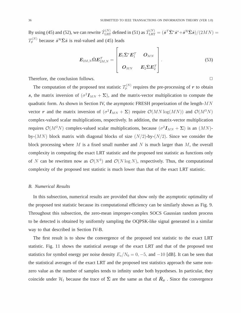
The computation of the proposed test statisticT(N)p requires the pre-processing ofr to obtain

s, the matrix inversion of(σ2IMN + Σ), and the matrix-vector multiplication to compute the

quadratic form. As shown in Section IV, the asymptotic FRESHproperization of the length-MN

vector r and the matrix inversion of(σ2IMN + Σ) requireO(MN log(MN)) and O(M3N)

complex-valued scalar multiplications, respectively. Inaddition, the matrix-vector multiplication

requiresO(M2N) complex-valued scalar multiplications, because(σ2IMN + Σ) is an (MN)-

by-(MN) block matrix with diagonal blocks of size(N/2)-by-(N/2). Since we consider the

block processing whereM is a fixed small number andN is much larger thanM , the overall

complexity in computing the exact LRT statistic and the proposed test statistic as functions only

of N can be rewritten now asO(N3) andO(N logN), respectively. Thus, the computational

complexity of the proposed test statistic is much lower thanthat of the exact LRT statistic.

B. Numerical Results

In this subsection, numerical results are provided that show only the asymptotic optimality of

the proposed test statistic because its computational efficiency can be similarly shown as Fig. 9.

Throughout this subsection, the zero-mean improper-complex SOCS Gaussian random process

to be detected is obtained by uniformly sampling the OQPSK-like signal generated in a similar

way to that described in Section IV-B.

The first result is to show the convergence of the proposed test statistic to the exact LRT

statistic. Fig. 11 shows the statistical average of the exact LRT and that of the proposed test

statistics for symbol energy per noise densityEs/N0 = 0,−5, and−10 [dB]. It can be seen that

the statistical averages of the exact LRT and the proposed test statistics approach the same non-

zero value as the number of samples tends to infinity under both hypotheses. In particular, they

coincide underH1 because the trace ofΣ are the same as that ofRx . Since the convergence


0 50 100

0.1

0.2

0.3

0.4

0.5

0.6

N

aver

aged

test

stati

stic

(a) H0

0 50 100

0.1

0.2

0.3

0.4

0.5

0.6

N

aver

aged

test

stati

stic

(b) H1

proposedexact LRT

0 [dB]

−5 [dB]

−10 [dB]

0 [dB]

−5 [dB]

−10 [dB]

Fig. 11. Statistical averages of the exact LRT and the proposed test statistics versusN for Es/N0 = 0,−5, and−10 [dB],

under (a)H0 and (b)H1.

w.p. 1 is hard to show by using Monte-Carlo simulations, we insteadshow the convergence in

probability that is implied by the convergence w.p.1 [31]. Fig. 12 shows the empirical cumulative

distribution function (CDF) of the difference of the proposed test statistic from the exact LRT

statistic for symbol energy per noise densityEs/N0 = −5 [dB] and N = 100, 200, and 400,

where the empirical CDF is obtained by105 Monte-Carlo runs. It can be seen that, as implied

by Theorem 4, the empirical CDF of the difference quickly converges to the unit step function

as the number of samples increases under both hypotheses.

The second result is to compare the receiver operating characteristic (ROC) curves of the

optimal detector that uses the exact LRT statistic (47) and the proposed detector that uses the


−0.01 −0.005 0 0.005 0.010

0.1

0.2

0.3

0.4

0.5

0.6

0.7

0.8

0.9

1

T(N )p − T

(N )LRT

empir

icalC

DF

(a) H0

−0.01 −0.005 0 0.005 0.010

0.1

0.2

0.3

0.4

0.5

0.6

0.7

0.8

0.9

1

T(N )p − T

(N )LRT

empir

icalC

DF

(b) H1

N=100N=200N=400

N=100N=200N=400

Fig. 12. Empirical CDFs of the difference of the proposed test statistic from the exact LRT statistic forN = 100, 200, and

400, under (a)H0 and (b)H1.

proposed test statistic (49). As a common practice in computing the PDF of a quadratic function

of Gaussian random vectors [32], we approximate the statistics by gamma random variables

to obtain the probability of missPM , Pr(declareH0|H1) and the probability of false alarm

PFA , Pr(declareH1|H0). The CDFFX(x; a, b) of the gamma random variableX with two

parametersa and b is given by

FX(x; a, b) = I

(

ax√b, b− 1

)

, ∀x > 0, (54)

where the Pearson’s form of incomplete gamma functionI(u, p) is defined by

I(u, p) ,1

Γ(p+ 1)

∫ u√p+1

0

tpe−tdt, (55)


10−4

10−3

10−2

10−1

100

10−4

10−3

10−2

10−1

100

pro

babilit

yofm

iss,

PM

probability of false alarm, PF A

proposed (theoretical)proposed (simulated)optimal (theoretical)optimal (simulated)

N = 10

N = 100

N = 250

Fig. 13. ROC curves of the optimal and the proposed detectors.

and where the gamma functionΓ(x) is defined byΓ(x) ,∫∞0

tx−1e−tdt [31]. Note that the

mean and the variance of the random variable whose CDF isFX(x; a, b) are given byab and

ab2, respectively. Thus,PM andPFA of the optimal and the proposed detectors can be computed

by using the conditional means and variances of the statistics underH0 andH1. Fig. 13 shows

the ROC curves of the optimal and the proposed detectors for symbol energy per noise density

Es/N0 = −5 [dB] andN = 10, 100, and250, where the theoretical results are evaluated by using

(54) while the simulated results are obtained from105 Monte-Carlo runs. It can be seen that

the performance of the detectors is accurately approximated by using the gamma distributions.

It can be also seen that the proposed detector performs almost the same as the optimal detector

does even whenN = 10.


VI. CONCLUSIONS

In this paper, the asymptotic FRESH properizer is proposed as a pre-processor for the block

processing of a finite number of consecutive samples of a DT improper-complex SOCS random

process. It turns out that the output of this pre-processor can be well approximated by a proper-

complex random vector that has a highly structured frequency-domain covariance matrix for

sufficiently large block size. The asymptotic propriety of the output allows the direct application

with negligible performance degradation of the conventional signal processing techniques and

algorithms dedicated to the block processing of proper-complex random vectors. Moreover, the

highly-structured frequency-domain covariance matrix ofthe output facilitates the development

of low-complexity post-processors. By solving the signal estimation and signal presence detection

problems, it is demonstrated that the asymptotic FRESH properizer leads to the simultaneous

achievement of computational efficiency and asymptotic optimality. Further research is warranted

to apply this pre-processor to various communications and signal processing problems involving

the block processing of a DT improper-complex SOCS random process and to derive such almost

optimal low-complexity post-processors.

REFERENCES

[1] F. D. Neeser and J. L. Massey, “Proper complex random processes with applications to information theory,”IEEE Trans.

Inf. Theory, vol. 39, no. 4, pp. 1293-1302, July 1993.

[2] P. J. Schreier and L. L. Scharf, “Second-order analysis of improper complex random vectors and processes,”IEEE Trans.

Signal Process., vol. 51, no. 3, pp. 714-725, Mar. 2003.

[3] P. Wahlberg and P. J. Schreier, “Spectral relations for multidimentional complex improper stationary and (almost)

cyclostationary processes,”IEEE Trans. Inf. Theory, vol. 54, no. 4, pp. 1670-1682, Apr. 2008.

[4] G. Taubock, “Complex-valued random vectors and channels: Entropy, divergence, and capacity,”IEEE Trans. Inf. Theory,

vol. 58, no. 5, pp. 2729-2744, May 2012.

[5] P. J. Schreier and L. L. Scharf,Statistical Signal Processing of Complex-Valued Data: TheTheory of Improper and

Noncircular Signals. NY: Cambridge Univ. Press, 2010.

[6] B. Picinbono and P. Chevalier, “Widely linear estimation with complex data,”IEEE Trans. Signal Process., vol. 43, no. 8,

pp. 2030-2033, Aug. 1995.

[7] W. M. Brown and R. B. Crane, “Conjugate linear filtering,”IEEE Trans. Inf. Theory, vol. 15, no. 4, pp. 462-465, July

1969.

[8] E. Serpedin, F. Panduru, I. Sari, and G. B. Giannakis, “Bibliography on cyclostationarity,”Signal Process., vol. 85, no.

12, pp. 2233-2303, Dec. 2005.

[9] W. A. Gardner, A. Napolitano, and L. Paura, “Cyclostationarity: Half a century of research,”Signal Process., vol. 86, no.

4, pp. 639-697, Apr. 2006.


[10] W. A. Gardner and L. E. Franks, “Characterization of cyclostationary random signal processes,”IEEE Trans. Inf. Theory,

vol. 21, no. 1, pp. 4-14, Jan. 1975.

[11] W. A. Gardner, “Signal interception: A unifying theoretical framework for feature detection,”IEEE Trans. Commun., vol.

36, no. 8, pp. 897-906, Aug. 1988.

[12] W. A. Gardner and C. M. Spooner, “Signal interception: Performance advantages of cyclic-feature detectors,”IEEE Trans.

Commun., vol. 40, no. 1, pp. 149-159, Jan. 1992.

[13] W. A. Gardner, W. A. Brown, and C.-K. Chen, “Spectral correlation of modulated signals: Part II–Digital modulation,”

IEEE Trans. Commun., vol. 35, no. 6, pp. 595-601, June 1987.

[14] W. A. Gardner and W. A. Brown, “Frequency-shift filtering theory for adaptive co-channel interference removal,” inProc.

23rd Asilomar Conf. Signals, Systems, Computers, vol. 2, Pacific Grove, CA, 30 Oct.- 1 Nov. 1989, pp. 562-567.

[15] G. B. Giannakis, “Filterbanks for blind channel identification and equalization,”IEEE Signal Process. Lett., vol. 4, no. 6,

pp. 184-187, June 1997.

[16] A. Sabharwal, U. Mitra, and R. Moses, “MMSE receivers for multirate DS-CDMA systems,”IEEE Trans. Commun., vol.

49, no. 12, pp. 2184-2197, Dec. 2001.

[17] J. H. Cho, “Joint transmitter and receiver optimization in additive cyclostationary noise,”IEEE Trans. Inf. Theory, vol. 50,

no. 12, pp. 3396-3405, Dec. 2004.

[18] Y. H. Yun and J. H. Cho, “An optimal orthogonal overlay for a cyclostationary legacy signal,”IEEE Trans. Commun., vol.

58, no. 5, pp. 1557-1567, May 2010.

[19] B. W. Han and J. H. Cho, “Capacity of second-order cyclostationary complex Gaussian noise channels,”IEEE Trans.

Commun., vol. 60, no. 1, pp. 89-100, Jan. 2012.

[20] W. A. Gardner, “Cyclic Wiener filtering: Theory and method,” IEEE Trans. Commun., vol. 41, no. 1, pp. 151-163, Jan.

1993.

[21] B. W. Han and J. H. Cho, “Optimal signaling in second-order cyclostationary Gaussian jamming environment,” inProc.

of IEEE Military Communications Conf. (MILCOM), Baltimore, MD, 7-10 Nov. 2011, pp. 102-107.

[22] J. Eriksson and V. Koivunen, “Complex random vectors and ICA models: Identifiability, uniqueness, and separability,”

IEEE Trans. Inf. Theory, vol. 52, no. 3, pp. 1017-1029, Mar. 2006.

[23] R. M. Gray, “Toeplitz and circulant matrices: A review,” Found. Trends Commun. Inf. Theory, vol. 2, no. 3, pp. 155-239,

2006.

[24] Y. G. Yoo and J. H. Cho, “Asymptotically optimal low-complexity SC-FDE in data-like co-channel interference,”IEEE

Trans. Commun., vol. 58, no. 6, pp. 1718-1728, June 2010.

[25] J. H. Yeo and J. H. Cho, “Properization of second-Order cyclostationary random processes and its application to signal

presence detection,” inProc. IEEE Military Communications Conf. (MILCOM), Orlando, FL, 29 Oct.-1 Nov. 2012, pp.

1-6.

[26] B. Picinbono and P. Bondon, “Second-order statistics of complex signals,”IEEE Trans. Signal Process., vol. 45, no. 2,

pp. 411-420, Feb. 1997.

[27] G. Bi and Y. Chen, “Fast generalized DFT and DHT algorithms,” Signal Process., vol. 65, no. 3, pp. 383-390, Mar. 1998.

[28] H. V. Poor,An Introduction to Signal Detection and Estimation, 2nd ed. NY: Springer-Verlag, 1994.

[29] A. van den Bos, “The multivariate complex normal distribution–A generalization,”IEEE Trans. Inf. Theory, vol. 41, no.

2, pp. 537-539, Mar. 1995.


[30] W. Zhang, H. V. Poor, and Z. Quan, “Frequency-domain correlation: An asymptotically optimum approximation of quadratic

likelihood ratio detectors,”IEEE Trans. Signal Process., vol. 58, no. 3, pp. 969-979, Mar. 2010.

[31] A. Papoulis,Probability, Random Variables, and Stochastic Processes, 4th ed. New York: McGraw-Hill, 2002.

[32] U. Grenander, H. O. Pollak, and D. Slepian, “The distribution of quadratic forms in normal variates: A small sample

theory with applications to spectral analysis,”J. Soc. Ind. Appl. Math., vol. 7, no. 4, pp. 374-401, Dec. 1959.

submitted to ieee transactions on … · cyclostationary random processes ... it is well known that...

Documents