submitted to ieee transactions on communications, …

SUBMITTED TO IEEE TRANSACTIONS ON COMMUNICATIONS, REVISED VERSION 1

Performance Analysis of an OFDMA

Transmission System in a Multi-Cell

EnvironmentSophie Gault, Walid Hachem(∗), and Philippe Ciblat

Abstract

The paper deals with design and performance analysis of Orthogonal Frequency Division Multiple

Access (OFDMA) based downlink cellular wireless communications. Due to a high degree of users

mobility, the Base Station is assumed to have only a statistical knowledge of the users channels. Relying

on the ergodic capacities connected to the user rates, a sub-carrier and power allocation that minimizes

the total transmitted power is proposed. The allocation strategy requires only the knowledge of the

channel statistics and the rate requirements for all users. An extension and a performance analysis of

this allocation algorithm in a multi-cell environment working with a frequency re-use factor equal to one

is also conducted. A condition for the multi-cell network to be able to satisfy all rate requirements is

derived.

Index Terms

Ergodic Capacity, Frequency Hopping, Multi-Cell Interference, OFDMA, Power and Sub-Carrier

Allocation.

I. INTRODUCTION

In wireless multi-user communications, Orthogonal Frequency Division Multiple Access (OFDMA) is

a technique that combines discrete multi-carrier modulation with a frequency division multiple access

(∗) Corresponding author.Sophie Gault ([email protected]) and Walid Hachem ([email protected]) were

with Supelec, Telecommunications Department, Plateau de Moulon, 91192 Gif-sur-Yvette, France. Philippe

Ciblat ([email protected]) is with Ecole Nationale Superieure des Telecommunications (ENST),

Departement Communications et Electronique, 46, rue Barrault, 75013 Paris, France.

August 30, 2006 DRAFT


based on the dynamic allocation of sub-carriers to users. The advantages of OFDMA include the flexibility

in sub-carrier attribution, the absence of multi-user interference due to sub-carrier orthogonality, and the

simplicity of the receiver. An OFDM modulation associated with a Frequency-Hopping (FH) multiple

access technique can be also viewed as a spread spectrum technique. Consequently FH-OFDMA offers

the advantage of averaging interference as in a CDMA system and thus enables us to construct a cellular

network with a frequency re-use factor between the adjacent cells equal to one [1], [2]. Thanks to these

advantages, OFDMA receives a great deal of attention as a candidate for future wireless communication

standards. Yet, the problem of the optimum sub-carrier and power attribution to users as well as the

robustness of OFDMA to inter-cell interference in a multi-cell setting are not fully understood. This

paper is a contribution toward solving these problems for downlink communications.

The power and sub-carrier allocation problem for OFDMA has been addressed by a number of contribu-

tions, among which [3]–[9] can be cited. These contributions assume the transfer functions of all users

channels as being known to the Base Station (BS). In a multi-cell setting, [10], [11] propose solutions

that involve coordination between Base Stations through the existence of a radio network controller that

gathers all channels state information in order to solve globally the sub-carrier allocation problem. In

this paper, we assume that these transfer functions are not available at the BS due to a high degree of

users mobility, and for computational complexity reasons, that Base Stations do not cooperate. Assuming

that the channels are random and frequency selective and that the BS has only a statistical knowledge

of these channels, the general problem that we address is the following: given the data rates required

by the users, the BS has to find the optimum number of sub-carriers and power per user in such a way

that the rate requirements of all users are satisfied and at the same time the total transmitted power is

minimum. Due to the time and frequency diversity of the users channels and to the non availability of

the channels transfer functions at the BS site, we consider that a relevant measure of the achievable rate

between the BS and a user is the so-called ergodic capacity. In practice, through frequency hopping, the

signal sent to a given user within a data frame visits a large number of this user’s channel states and

benefits from an averaging effect over the corresponding gains. This justifies the use of ergodic capacity

as a performance measure.

One advantage of minimizing the BS transmitted power is to mitigate the interference that disturbs the

neighboring cells. Nevertheless, this so-called Multi-Cell Interference (MCI) still represents a fundamental

obstacle against a possible increase of the whole cell capacity. In the second part of the paper, we analyze

thoroughly the impact of Multi-Cell Interference over the system performance. For a BS of interest, a

simple way to combat the MCI that comes from the neighboring cells, is to increase its own transmitted



power. Consequently, in turn, the neighboring Base Stations will also have to increase their powers. If

the system is to work, this process should converge. This leads to the issue of the whole system stability.

In order to be able to conduct our performance analysis under the presence of MCI, and in particular,

to derive a condition for the system stability, we begin by assuming that the number of users in a cell

and the signal bandwidth grow both toward infinity in such a way that the total rate (or capacity) of the

BS per channel use1 converges toward a constant. A parameter of prime importance will emerge from

our analysis : this is the mean rate per channel use and per cell volume unit required by the users in

a cell. By considering an idealized network where all cells are identical and regularly spaced, we show

that the network is stable if this rate is less than a given threshold. An analysis of this threshold in terms

of certain system parameters like the cell radius and the power decay profile will also be conducted.

In section II, we state the allocation problem for the single cell case. Section III is devoted to the solution

of the power and sub-carrier optimization problem, that shows to be solvable by means of a Lagrangian

formulation. The asymptotic regime in the number of users introduced above is described rigorously in

section IV. Under this regime, the issues of performance in presence of MCI and network stability are

addressed in section V. Finally, section VI is devoted to the numerical illustrations of the results. We

also compare the multi-cell OFDMA approach with an OFDMA technique assigning different sets of

sub-carriers to adjacent cells and thus working with a frequency re-use factor less than one.

In the paper, E[.] will denote the expectation operator. The (multivariate) complex-valued circular Gaussian

distribution with mean a and covariance matrix Σ will be denoted CN (a,Σ).

II. SINGLE CELL MODEL

We consider a downlink transmission where a BS serves K users. The users channels are time

varying frequency selective channels. The transmitted signal is parsed into frames, each corresponding

to an OFDM (Orthogonal Frequency Division Multiplexing) symbol of duration T seconds. The channel

impulse response of user k, assumed invariant during OFDM symbol m, is represented during this symbol

by the vector hk(m) = [hk (m, 0) , . . . hk (m,L− 1)]T where L is an upper bound on the users channel

lengthes. Denoting by N the number of sub-carriers in an OFDM symbol (equivalently the number

of channel uses per OFDM symbol), let Hk(m) = [Hk(m, 0), . . . ,Hk(m,N − 1)]T be the vector that

represents the transfer function of the channel of user k at the N Fourier frequencies of OFDM symbol

m. In other words, Hk(m) =√NFN,Lhk(m) where FN,L is the N × L Fourier matrix which (n, l)

1The capacity per channel use is the capacity divided by the channel bandwidth



entry is given by [F]n,l = 1√N

exp (−2iπnl/N) for n = 0, . . . , N − 1 and l = 0, . . . , L− 1. The signal

Yk(m,n) received by user k at sub-carrier n after the Discrete Fourier Transformation of OFDM symbol

m writes then

Yk(m,n) = Hk(m,n)S(m,n) + Vk(m,n) (1)

where S(m,n) is the signal transmitted by the BS in the discrete Fourier domain and Vk(m,n) is

the additive noise received by user k at sub-carrier n of OFDM symbol m. We assume that the two

dimensional noise process Vk(m,n) is white, and that a sample of this process has the distribution

CN (0, σ2) where σ2 refers to the noise variance. Recall that this variance is written as σ2 = N0B

where N0 is the noise Power Spectral Density and B = N/T is the system bandwidth, or equivalently

the number of channel uses per second. We formulate the following assumption regarding the users

channels:

(A) The vector process hk(m) is a random process with distribution CN (0,Σk) where

Σk =

ς2k,0 0

. . .

0 ς2k,L−1

.

Assumption (A) states that the channel taps in the time domain are circular Gaussian and independent

but they do not have necessarily the same variances. A consequence of (A) is that all entries of Hk(m),

i.e., the transfer function coefficients in the discrete Fourier domain, have the distribution CN (0, ς 2k ) with

a variance ς2k =∑L−1

l=0 ς2k,l. The fact that they have the same variance ς2k can be verified by inspecting

the diagonal elements of the matrix E[

Hk(m)HHk (m)

]

= NFN,LΣkFHN,L. It results that the “Gain to

Noise Ratios” (GNR) Gk(m,n) = |Hk(m,n)|2 /N0 of user k for n ∈ {0, . . . , N − 1} and m ∈ Z are

identically distributed.

In the sequel, it will be assumed that the receiver of user k has the knowledge of its channel impulse

response and of its noise power. Alternatively, at the BS, only the K mean Gain to Noise Ratios ak given

by

ak = E [Gk(m,n)] = ς2k/N0 (2)

are assumed available. With these assumptions, we shall be interested all along this paper in the so-

called ergodic Shannon capacities of these channels. Recall that the ergodic capacity can be approached

by coding schemes that exploit properly the channel coherence bandwidth and/or its coherence time

which we shall assume in the sequel.

In order to state our problem clearly, we begin by assuming that there is only one user (K = 1)



communicating with the BS. To be able to reach the capacity, the transmitter has to send independent

centered Gaussian signals over the N sub-carriers. In our case, since the random variables Gk(m,n)

are identically distributed, the capacity is reached when these Gaussian signals have the same variances.

Assume that the user requires a rate of ρ1 bits per channel use and denote by E1 the minimum transmitted

energy per channel use needed to satisfy this rate requirement. Then E1 satisfies ρ1 = E [log (1 +E1G1)]

where G1 is a random variable that has the same probability distribution as any of the random variables

Gk(m,n) and the expectation is taken with respect to this random variable. Note that the part of the

energy devoted to the guard interval is neglected in this expression.

Let us turn now to the case where K > 1. In this paper we restrict ourselves to a sub-optimal user share

strategy in information-theoretic point of view. Indeed, we focus on OFDMA scheme which means that

for any sub-carrier n and OFDM symbol m, the signal S(m,n) is allocated to a single user. We denote

by γk the sharing factor associated with user k. The factor γk provides the proportion of time-frequency

slots (m,n) for which S(m,n) is allocated to user k. By definition, we therefore have γk ≥ 0 and∑K

k=1 γk ≤ 1. Once the sharing factors {γ1, . . . , γK} are chosen, the practical allocation can be done in

several ways: in theory, at one extreme, one can imagine that a user is given a whole OFDM symbol from

time to time ; at the other extreme, a user is given some fixed subset of the N sub-carriers of cardinality

nk such that nk/N = γk up to a rounding error. In many practical situations, a more reasonable access

scheme consists in allocating sub-carriers to users according to some frequency hopping pattern [12].

Here, this pattern will be designed in such a way that constraints associated with the sharing factors γk

are respected.

Let Ek = E

[

|S(m,n)|2]

/B be the energy transmitted on the sub-carrier n of OFDM symbol m when

the slot (m,n) is destined to user k. The ergodic capacity per channel use Ck given to user k is then

Ck = γkE

[

log

(

1 +|Hk(m,n)|2BEk

σ2

)]

= γkE [log (1 +GkEk)] (3)

where Gk is a random variable that has the same distribution as Gk(m,n) and the expectation E is taken

with respect to the distribution of Gk. Denoting by Qk the mean energy per channel use sent to user k,

we have Qk = γkEk. The mean energy per channel use Q transmitted by the BS is then

Q =

K∑

k=1

Qk . (4)

Our problem is then the following : given a rate vector ρ = [ρ1, . . . , ρk]T where ρk is the capacity per

channel use required by user k, find the energies {Ek} and the sharing factors {γk} such that the total



transmitted energy Q is minimum. Formally, this problem is written : minimize Q with the constraints

−Ck + ρk ≤ 0 for k = 1, . . . ,K (5)K∑

k=1

γk − 1 ≤ 0 . (6)

The capacity Ck given by Equation (3) is not a convex nor a concave function of (γk, Ek). However, by

writing

Ck = γkE

[

log

(

1 +GkQk

γk

)]

, (7)

it appears that Ck is a concave function of (γk, Qk). Indeed, consider the function f(x, y) = x log(1+y/x)

defined on R2+. As the eigenvalues of the 2×2 Hessian matrix associated with f(x, y) are 0 and − x2+y2

x(x+y)2 ,

this function is concave. It results that Ck = E [f (γk, GkQk)] is concave.

In the next section, we will minimize the cost function (4) under the constraints (5-6) by using the

Lagrangian multipliers.

III. THE ALLOCATION ALGORITHM

Our constrained minimization problem (5-6) is convex in the vector parameter x =[

qT,γT]T where

q = [Q1, . . . , QK ]T and γ = [γ1, . . . , γK ]T. The Lagrange-KKT conditions are then written

∇xQ−K∑

k=1

λk∇xCk + β∇x

(

K∑

k=1

γk

)

= 0 (8)

where ∇x denotes the gradient operator with respect to the vector x, the positive real numbers λ1, . . . , λK

are the Lagrange multipliers associated with constraints (5) and the positive number β is the Lagrange

multiplier associated with the constraint (6). The multi-variate equation (8) can be rewritten as the set

of 2K scalar equations λk∂Ck/∂Qk = 1 and λk∂Ck/∂γk = β for k = 1, . . . ,K . By developing the left

hand members of these Equations, we obtain

λkE

[

Gk

1 +GkEk

]

= 1 (9)

λkE

[

log (1 +GkEk) −GkEk

1 +GkEk

]

= β (10)

for k = 1, . . . ,K . By plugging Equations (9) into (10) we have

f1(E1) = f2(E2) = · · · = fK(EK) = β (11)

where

fk(x) =E

[

log (1 + xGk) − xGk

1+xGk

]

E

[

Gk

1+xGk

] =E [log (1 + xGk)]

E

[

Gk

1+xGk

] − x . (12)



Let us inspect the middle member of this expression. For every a > 0, the function ga(x) = log(1 +

ax) − ax/(1 + ax) increases from zero to infinity as x increases from zero to infinity. Therefore, the

numerator increases from zero to infinity with x. As the denominator decreases with x, the function fk(x)

increases from zero to infinity over the interval [0,∞) as shown on figure 1. The allocation algorithm

.

β

E2 E1 EK

x

fK(x)

f1(x)

f2(x)

0.

Fig. 1. Shapes of functions fk(x) and evolution of energies vs β

is the following: initialize β to a value close to zero. Compute the energies Ek by solving numerically

Equations (11). To obtain the rate ρk, user k needs the sharing factor γk(β) given by

γk(β) =ρk

E [log (1 +GkEk(β))](13)

where Ek(β) are the solutions of Equations (11). If β is too small, the energies Ek(β) will be too small

also and we will have∑K

k=1 γk(β) > 1. Increase β until∑K

k=1 γk(β) = 1 is satisfied.

Let us give the expressions of the allocated energies and sharing factors with respect to the GNRs ak.

Since the random variables Hk(m,n) are circular Gaussian, Gk has the exponential distribution with

mean ak. Let Xe be a positive random variable with the probability density e−t, and let f(x) be the

function defined on [0,∞) as

f(x) =E [log (1 + xXe)]

E

[

Xe

1+xXe

] − x =

∫

log (1 + xt) e−tdt∫

t1+xte

−tdt− x =

e1/xx2Ei (1/x)

x− e1/xEi (1/x)− x

where Ei is the so-called exponential integral function, defined as Ei(x) =∫∞x

e−t

t dt for x > 0.

As Gk is exponentially distributed with mean ak, it has the same distribution as akXe. Therefore, from

Equation (12), we have

fk(x) =1

akf(akx) .



Powers attribution connected to equations (11) can then be written

Ek(β) =1

akf (−1)(akβ) (14)

where f (−1) defined on [0,∞) is the inverse of f with respect to composition. Thanks to Eq. (14), Eq.

(13) can be rewritten as follows

γk(β) =ρk

F (akβ)(15)

where F (x) is the function defined on R+ by

F (x) = E

[

log(

1 +Xef(−1)(x)

)]

.

It can be shown that F (x) increases from zero to infinity as x increases from zero to infinity. Moreover,

F (x) is continuous on R∗+.

Since∑K

k=1 γk(β) = 1, the multiplier β is the unique solution to the following equationK∑

k=1

ρk

F (akβ)= 1 . (16)

It will also be useful to give the expression of Q. It writes

Q =K∑

k=1

ρk

ak

1

F (akβ)f (−1)(akβ) . (17)

We obtained an implicit closed-form expression for the minimal energy per channel use that enables us

to ensure a rate ρk for user k in a single cell environment.

IV. ASYMPTOTIC ANALYSIS

The purpose of this section is to give an asymptotic expression of the transmitted energy per channel

use (16,17) in the asymptotic regime where the number of users K in the cell grows toward infinity. Our

aim is to obtain more tractable expressions that will be useful in particular in the multi-cell situation

described in the next section. Assume that user k requires a rate of Rk nats per second. As the number of

users grows to infinity, the total required rate R(K) =∑K

k=1Rk grows to infinity. In order to accommodate

all the users, we shall assume that the bandwidth B also grows to infinity. The asymptotic regime will

therefore be characterized by the fact that K → ∞, B → ∞, and K/B → α where α is a positive

constant. Note that in this regime, the capacities per channel use (i.e., the spectral efficiencies) of the

different users ρk = Rk/B go to zero.

In order to ensure the convergence of the transmitted energy per channel use in the asymptotic regime and

to obtain asymptotic expressions that can be interpreted simply, some additional hypotheses are required.



The cell can be identified with a compact C included in R or in R2 according to whether the cell is one

or two dimensional. It is frequent to model the GNR ak as being directly related to the location xk of

mobile k. Here, xk is a one or two dimensional variable that represents a point of C in a coordinate

system which origin is occupied by the BS. Getting back to Equation (2), the variance ς 2k will be written

as ς2k = q(xk) where q(x) is a continuous function from C to R∗+ used to model the so called path loss.

With this model, we have ak = π(xk) where π(x) is the GNR profile defined as π(x) = q(x)/N0. One

widely used example for q(x) is q(x) = |x|−s where |x| denotes the distance between the mobile and

the BS, and s is a positive parameter that characterizes the rate of decrease of the signal power with

distance. Remember that q(x) is assumed to be defined on C. Therefore, if q(x) = |x|−s is considered,

the origin has to be excluded from C. In this situation, it is often assumed that C = [−D,−d]∪ [d,D] in

the one dimensional case, and C is the closed annulus delimited by circles with radii d and D where d

and D are two real numbers such that 0 < d < D.

The two parameters of user k required to implement the allocation algorithm (14–16) are ρk = Rk/B

and ak = q(xk). By consequence, the user configuration can be equivalently characterized by the set of

couples {(Rk, xk)}k=1,...,K . Describing the set of parameters {(Rk, xk)}k=1,...,K is equivalent to providing

the following positive measure ν(K) acting on the Borel sets of R+ × R+

ν(K)(u, x) =1

K

K∑

k=1

δRk ,xk(u, x)

where δRk ,xkis the Dirac measure at the point (Rk, xk). It is realistic to assume that all required rates

belong to an interval ∆R = [Rmin, Rmax] of R∗+. By consequence, for every K > 0, the support of

ν(K) is included in the compact set ∆ = ∆R × C. Notice that ν(K) is a positive measure satisfying∫

∆ dν(K) = 1, and as such, it is a probability measure. Using the fact that ρk = Rk/B, Equations (16)

and (17) can be rewritten respectively as

K

B

∫

∆

u

F (π(x)β(K))dν(K)(u, x) = 1 (18)

and

Q(K) =K

B

∫

∆

u

π(x)

f (−1)(π(x)β(K))

F (π(x)β(K))dν(K)(u, x) . (19)

In the last expression, the notation Q(K) is used instead of Q to put ahead the fact that we now have a

sequence of energies per channel use indexed by the number of users. The multiplier β is denoted β (K)

similarly. Convergence of this sequence will come from the following assumption:

(B1) As K → ∞, the sequence of measures ν (K) converges weakly to a probability measure ν.



It is realistic to assume that the limit joint distribution ν of rates and users locations is the measure

product of a limit rate distribution times a limit location distribution. This is justified heuristically by a

notion of independence between the rate requirements of the users and their locations:

(B2) The measure ν satisfies dν(u, x) = dζ(u) × dλ(x) where ζ is the limit distribution of rates and λ

is the limit distribution of the user locations xk. Both ζ and λ are probability measures. Here ×denotes the product of measures.

Typically, the measure λ can be modeled as the uniform probability measure over C, in other words

dλ(x) = (1/|C|) dx where |C| is the cell volume. Concerning the limit rate distribution ζ , denote by

R =∫

∆R

udζ(u) its mean. A parameter that will be of prime importance in the following is the mean

rate r per channel use and per cell volume unit. It is given by r = αR/|C| nats per channel use and per

(squared) meter.

We turn now to the asymptotic expressions. We have the following theorem:

Theorem 1: Assume K → ∞ in such a way that K/B → α > 0, and that the measure ν (K) satisfies

assumptions (B1) and (B2). Assume that π(x) is continuous and satisfies π(x) > 0 on C. Then Q(K)

converges to Q given by

Q = r

∫

C

f (−1)(π(x)β)

π(x) F (π(x)β)|C|dλ(x) (20)

where β is the unique positive number that satisfies

r

∫

C

|C|F (π(x)β)

dλ(x) = 1. (21)

This theorem which proof is in Appendix A is the main result of the paper in the single cell environment.

One interesting consequence of Theorem 1 is that the rate distribution affects the asymptotic energy

per channel use through its mean only. On other words, in the asymptotic regime, the minimal power

consumed for achieving the individual user rates depends only on the global rate requirement. It does

not depend on the particular form of the individual rate distribution.

V. THE MULTI-CELL ENVIRONMENT

In GSM mobile cellular system, the spectrum is split into several sub-bands, and adjacent cells do not

share the same sub-band. Consequently there is no multi-cell interference coming from adjacent cells.

But such a system requires a frequency planning and prevents soft handover. Therefore advanced cellular

systems (e.g., UMTS) will work with an universal frequency re-use to take benefit of the soft handover,

of the macro-diversity, and of a flexible frequential management. To carry out an universal frequency



re-use system, any spread-spectrum based multiple acces technique, such as DS-CDMA or FH-OFDMA,

can be employed [13].

Consequently, in this section, we modify and analyze the behavior of the power allocation algorithm

in a multi-cell environment, i.e. when, in addition to the background noise, the signal received by a user

is corrupted by the signals sent by the Base Stations of other cells. We prove that the power allocation

strategy is quite different from the single cell case and especially there exists a maximum value for the

rate. Beyond this threshold, the multi-cell interference strongly disturbs the transmission and does not

enable us to get reliable transmission.

A. Cell Model

We consider for simplicity a one dimensional cellular system that consists of a linear regular array

of cells as shown in figure 2. In this figure, D is the half distance between two neighboring BS, and

a cell is included in the interval [−D,D] if we identify its BS with the origin. Even if such a multi-

cell model, studied in [14] and [15] is an ideal model, it provides some interesting guidelines that help

to implement a practical cellular system. Here, to simplify our presentation, we furthermore assume

that the Multi-Cell Interference (MCI) comes from the adjacent cells only; we thus neglect the MCI

due to further cells. Suppose that, at OFDM symbol m, the signal sent by the BS on sub-carrier n is

.2D − x

2D + x

D

x

DD D

Cell c Cell c + 1Cell c − 1

.

Fig. 2. The multi-cell environment

intended to user k. In a single cell environment, the received signal Yk(m,n) is then written Yk(m,n) =

Hk(m,n)S(m,n) +Vk(m,n) as shown in Equation (1). To give the expression of the received signal in

a multi-cell environment, let us number the cells as indicated in the figure and put the superscript (c) to

refer to the quantities located to cell number c. For instance the signal transmitted by BS number c will

be denoted S(c)(m,n). Consistently with the notations of section II, we denote by h(c′,c)k (m) the impulse



response of the channel that carries the signal of BS number c′ to user k of cell c, and by H(c′,c)k (m)

its Discrete Fourier Transform. With these notations, the signal received by user k of cell c at OFDM

symbol m and sub-carrier n becomes

Y(c)k (m,n) = H

(c)k (m,n)S(c)(m,n)+H

(c−1,c)k (m,n)S(c−1)(m,n)+H

(c+1,c)k (m,n)S(c+1)(m,n)+V

(c)k (m,n) .

(22)

We assume that a frequency hopping algorithm is implemented in all cells and that this algorithm ensures

that the signal of any user is equally distributed on all sub-carriers. It results from this assumption that

E

[

∣

∣S(c)(m,n)∣

∣

2]

= BQ(c) for all m and n. If we furthermore suppose that the inter-cell channels

h(c′,c)k (m) satisfy assumption (A), then the variance of H (c−1,c)

k (m,n) is independent of m and n as in

section II. In this case, the GNR a(c)k of user k in cell c is written

a(c)k =

E

[

∣

∣

∣H

(c)k (m,n)

∣

∣

∣

2]

Q(c−1)E

[

∣

∣

∣H

(c−1,c)k (m,n)

∣

∣

∣

2]

+Q(c+1)E

[

∣

∣

∣H

(c+1,c)k (m,n)

∣

∣

∣

2]

+N0

.

Let us consider the problem of the capacity derivation. The noise Vk(m,n) in Equation (1) is replaced in

the multi-cell case by the noise Vk(m,n) = H(c−1,c)k (m,n)S(c−1)(m,n)+H

(c+1,c)k (m,n)S(c+1)(m,n)+

V(c)k (m,n) as shown in Equation (22). As this noise is clearly non-Gaussian, the capacity is in general

difficult to derive. Nevertheless, if we endow S(c)(m,n) with the Gaussian distribution, then the associated

mutual information between S(c)(m,n) and Y (c)k (m,n) is a lower bound to the capacity. It is furthermore

well known that when the variances of the information signal and the noise are fixed and the information

signal is Gaussian, then the mutual information is minimum when the noise is Gaussian [16]. Therefore

we can easily derive a lower bound on the true capacity if we approximate the multi-cell interference

noise by a Gaussian noise with the same variance. Then we are essentially led back to the situation of

section II.

As we shall require this lower bound to satisfy the rate constraints, the obtained power will represent

an upper bound on the power necessary in theory to comply with these constraints.

In short, energies per channel use and shares are still computed according to Equations (14–16) with the

difference that ak is replaced by a(c)k . Note that the quantities a(c)

k can be consistently estimated by the

BS number c.

Let us now consider the asymptotic regime in the multi-cell situation. In order to apply a path-loss model

to the inter-cell channels, we extend the set of definition of the function q(x) to C ∪ (2D+C)∪ (2D−C)

where 2D ± C = {2D ± x, x ∈ C}, and assume that q(x) is continuous on this domain. With this



extension, we have E

[

∣

∣

∣H

(c−1,c)k (m,n)

∣

∣

∣

2]

= q(2D + x) and E

[

∣

∣

∣H

(c+1,c)k (m,n)

∣

∣

∣

2]

= q(2D − x) (see

figure 2). Let us denote by πQ(c−1),Q(c+1)(x) the GNR profile in the conditions described by Equation

(22). This function is written

πQ(c−1),Q(c+1)(x) =q(x)

Q(c−1)q(2D + x) +Q(c+1)q(2D − x) +N0.

In a multi-cell setting, a lower bound on the total energy per channel use is therefore given by Equation

(20) where β satisfies (21), and in both equations, π(x) is replaced by πQ(c−1),Q(c+1)(x).

B. The Equilibrium Energy per Channel Use

Any BS combats the MCI coming from its neighbors by increasing its own transmitted power. By doing

so, it will however increase the interference it produces with its neighboring cells, so that these cells will

have to increase in turn their powers, and so forth. In this section, we tackle the problem of finding a

condition under which the whole cell array can nevertheless reach an equilibrium. Here we consider an

infinite array and we assume that each cell satisfies the conditions of the asymptotic regime. To simplify

our analysis, we assume that at a certain moment that we call moment zero, all cells transmit at power

Q0B. For instance, one can imagine that moment zero is the moment where all BS are “switched on”

simultaneously, in which case one would have Q0 = 0. After executing the allocation algorithm, each

BS will transmit a signal with the energy per channel use given by Equation (20) that we denote here

Q1. At a later moment called moment one, the cells will execute again the algorithm simultaneously then

deliver the energy Q2. By iterating, the energy Qn+1 delivered by each BS at moment n will be given

by the following expressions. Let β(Q, r) be the unique solution to the equation (see Eqs (18) and (19))

r

∫

C

|C|F(

πQ(x)β(Q, r))dλ(x) = 1 (23)

where πQ(x) is given by

πQ(x) = πQ,Q(x) =q(x)

Q (q(2D + x) + q(2D − x)) +N0, (24)

and define ξ(Q, r) as

ξ(Q, r) = r

∫

C

f (−1)(

πQ(x)β(Q, r))

πQ(x) F(

πQ(x)β(Q, r)) |C|dλ(x) . (25)

ξ(Q, r) is the total energy per channel use a cell needs to transmit to attain the mean rate of r nats per

channel use and cell volume unit when its neighboring cells transmit at energy Q. The energy Qn+1 will

be given by

Qn+1 = ξ(Qn, r) . (26)



The convergence of this sequence is treated by the following theorem which is the main result of this

section:

Theorem 2: Let t(x) be defined on C as

t(x) =q(x)

q(2D − x) + q(2D + x).

Assume that t(x) is continuous and satisfies t(x) > 0 on C. Define ψ(r) on R∗+ as

ψ(r) = r

∫

C

f (−1)(t(x)b(r))

t(x)F (t(x)b(r))|C|dλ(x) (27)

where b(r) is the unique positive number that satisfies

r

∫

C

|C|F (t(x)b(r))

dλ(x) = 1 . (28)

Then

1) the equation ψ(r) = 1 admits an unique solution r0 > 0.

2) for any initial value Q0 ≥ 0, if r < r0, then the sequence (Qn) which elements are given by (26)

converges, and if r ≥ r0, then it grows to infinity.

This theorem can be proven thanks to the following three lemmas:

Lemma 1: For every r > 0, the function ξ(Q, r) defined in (25) satisfies the following properties:

ξ(0, r) > 0, ξ(Q, r) is increasing in the variable Q on R+, and ξ(Q, r)/Q is decreasing in Q on R∗+.

Lemma 2: limQ→∞ ξ(Q, r)/Q = ψ(r) where ψ is given by (27).

Lemma 3: limr→0 ψ(r) = 0 and limr→∞ ψ(r) = ∞. Furthermore r 7→ ψ(r) is increasing.

These lemmas are respectively proven in Appendices B, C, and D. Finally the proof of Theorem 1 is

drawn in Appendix E.

Practically this theorem indicates that

• If the rate is less than a certain threshold r0, then the multi-cell system can operate ;

• For a given achievable rate, i.e, a rate less than the threshold r0, the proposed allocation strategy

converges and minimizes the power consumption. Notice that this part of the theorem is similar to

the single cell case.

VI. NUMERICAL ILLUSTRATIONS

We begin by introducing the channel models that we considered. Simulations are carried out using

three different path loss exponent values: s = 2, 3 and 3.5 as introduced in section IV. We consider a Free

Space Loss (FSL) model characterized by a path loss exponent s = 2, and the so-called Okumura-Hata



(O-H) model for open areas, which is widely used for predicting path loss in mobile wireless systems (

[17]). For the O-H case, we consider the cases s = 3 and s = 3.5.

The carrier frequency is f0 = 1.8 GHz. At this frequency, the basic equations for path loss in dB are :

FSL : πIdB(xkm) = 20 log10(xkm) + 97.5

O-H s = 3 : πIIdB(xkm) = 30 log10(xkm) + 93.3

O-H s = 3.5 : πIIIdB(xkm) = 35 log10(xkm) + 103.8

where xkm is the distance in km between the BS and the receiver. The default values for the cell inner

radius d and outer radius D are set to 150 m and 5 km respectively. Finally, the signal bandwidth is

B = 5MHz and the noise Power Spectral Density is N0 = −170 dBm/Hz.

We first validate the asymptotic analysis in a single cell context with the FSL model. We consider a

mean rate request r of 0.5 bit per second per channel use and per kilometer and compare the power

QB required by our allocation algorithm (cf. (17)) for a number of users K varying between 5 and 100,

and the power Q(K)B required in asymptotic regime (cf. (20)). On Figure 3, we plotted the normalized

MSE, i.e., (Q−Q(K))2/(Q(K))2.

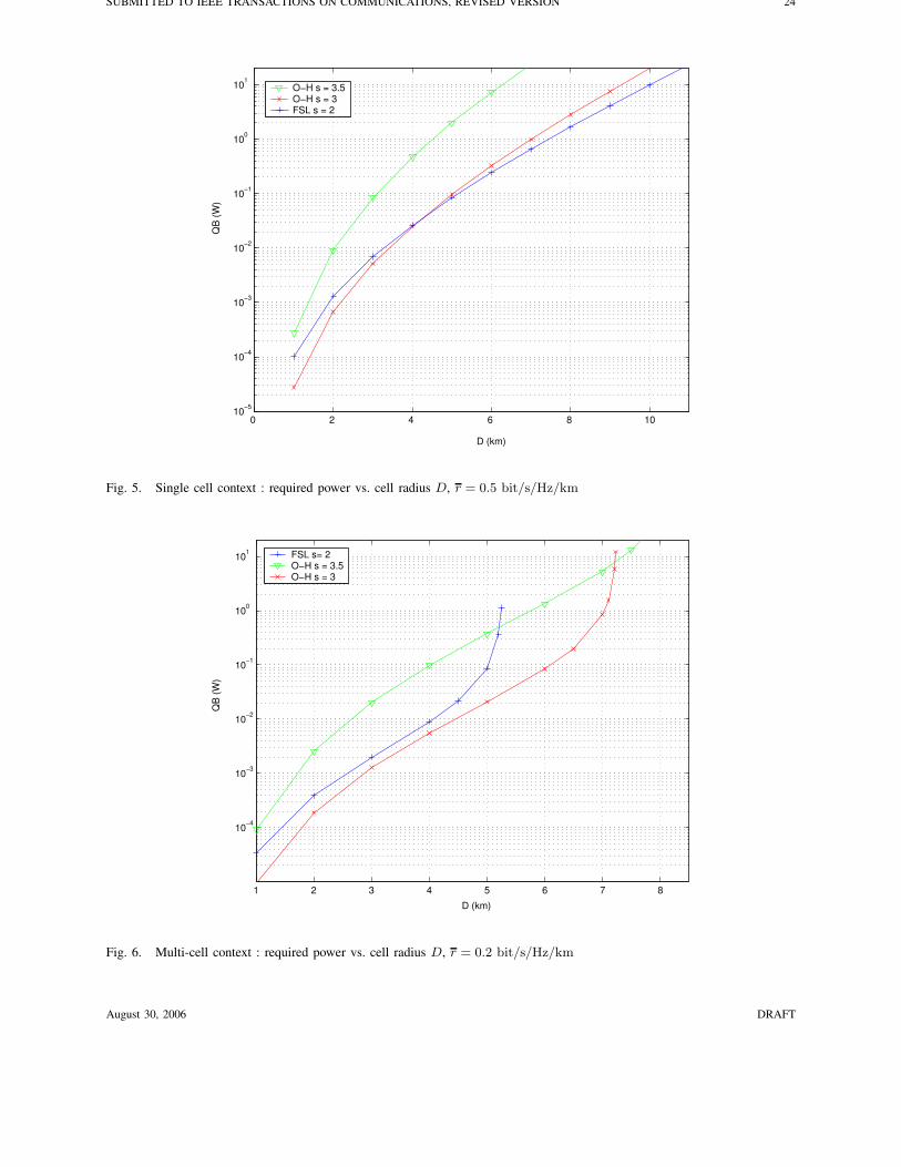
On Figures 4 and 5, we also compute the power required by the BS to reach a mean rate r of 0.2 and

0.5 bit per second, per channel use and per kilometer, versus the cell radius for various channel models

in the single cell context. We use the asymptotic approximations provided by Equations (20) and (21).

We assume that the transmitted power is limited to 20 W, which corresponds to the upper border of the

figures.

These curves give useful guidelines for cell dimensioning : given a constraint on the transmitted power,

we directly deduce the corresponding size of the cell that can be covered by the BS. For instance, if

the maximal transmitted power is 1 W, the cell radius can not be greater than 14 km for a mean rate

requirement of 0.2 bit/s/Hz/km under the FSL model. In the same conditions, the maximal radius

becomes 7.5 km for a mean rate value of 0.5 bit/s/Hz/km.

In a multi-cell environment, the BS coverage performance is seriously degraded by multi-cell interfer-

ence. In Figure 6, the mean required rate is set to r = 0.2 bit/s/Hz/km like for Fig. 4. Fig. 6 shows

that the maximal cell radius is reduced from 14 km to 5.4 km. Moreover, on Figure 7, the maximal cell

radius is shrinks from 7.5 km (see Fig. 5) to 2.2 km for a mean rate requirement of 0.5 bit/s/Hz/km.

Furthermore it is worth noticing a major difference between single-cell and multi-cell contexts : the curves

obtained in the multi-cell context grow to infinity when the cell radius D reaches a certain threshold.

This value depends on s and on r. For instance, in the free space model, for a mean rate requirement of



0.2 bits/s/Hz/m, a limit is located at D = 5.4 km.

To justify the existence of these limits, let us now focus on how the multi-cell results were obtained.

Figure 8 represents the function denoted ξ(Q, r) given by (25) for three different values of r. For

each value of Q, we first find β(Q, r) defined as the unique solution of Equation (23), and then we

compute ξ(Q, r). The equilibrium power is given by the fixed point coordinates which can be determined

geometrically by the intersection of ξ(Q, r) with the first bisector, shown as a solid line on the figure 8.

The values of Q corresponding to the different mean rate requirements are gathered in Table I. Q naturally

increases with r, and so does ψ(r). Therefore, as predicted by Theorem 2, there exists a limit on the

mean rate demand r0 beyond which ξ(Q, r) and the first bisector do not meet. Figure 9 represents r0

versus the cell radius in km for the three path loss models. For a given cell radius D, any mean rate

lower than r0 can be satisfied i.e., the algorithm converges for any r < r0. Symmetrically, to any mean

rate r, corresponds a maximal coverage radius D. As a consequence, for a given r, when D tends to the

corresponding limit radius, Q tends to infinity, which explains the presence of the asymptotes on Figures

6 and 7.

r (bit/s/Hz/km) QB (W)

0.15 1.08 × 10−2

0.2 8.55 × 10−2

0.21 0.95

TABLE I

EQUILIBRIUM POWER (INTERSECTION POINTS ON FIGURE 8)

Our FH-OFDMA allocation strategy is based on an universal frequency re-use (i.e., a frequency re-

use factor of one). It would be interesting to compare this allocation strategy to a strategy that assigns

different frequency bands to adjacent cells, which amounts to a frequency re-use factor of one half for

one dimensional cells. With a frequency re-use factor of one, more (macro and frequency) diversity can

be collected and the technical constraints due to frequency planning are avoided. In contrast, compared

to the strategy with frequency planning, the signal to noise ratio per sub-carrier degrades because of the

MCI. In Figure 10, we compare both strategies by plotting the consumed power versus the size of the

cell for a given mean required rate per cell volume. In the case of FH-OFDMA with a re-use factor of

one, we consider the mean rate r = 0.2bit/s/Hz/km and the power QB where B = 5MHz is the total



bandwidth used by the system. In order to ensure the same mean rate requirement per cell volume, the

approach with frequency planning is carried out by simply turning back to the single cell case (introduced

in Section II) and by considering the mean rate requirement r′ = 0.4bit/s/Hz/km and a power equal to

Q′B/2 where Q′ is obtained via Eq. (16) and (17).

We notice that the required power per BS without frequency planning is slightly smaller than the power

with frequency planning as long as the cell radius is smaller than a given threshold that depends on the

path loss exponent s. Beyond this threshold, frequency planning is better from the point of vue of total

consumed power. This threshold is equal to 3.2km, 5.6km, and 6.7km for s = 2, 3, and 3.5 respectively.

For reasonable values of cell radius, it is useless to implement frequency planning.

APPENDIX

A. Proof of Theorem 1

Because F (x) increases from zero to infinity on R+, it is clear that β is the unique solution of Equation

(21). We shall show that β(K) given by (18) converges to β. Equation (21) can be rewritten as

α

∫

∆

u

F (π(x)β)dν(u, x) = 1 . (29)

The function F (x) is continuous and strictly positive on any compact subset of R∗+. Due to the assumptions

on π(x), the function F (π(x)β) is continuous and satisfies F (π(x)β) > 0 on the compact set ∆ for

every β > 0. Therefore, for any β > 0, u/F (π(x)β) is continuous on ∆. By applying standard results

related to the convergence of measures [18], and by using (29), we therefore have

K

B

∫

∆

u

F (π(x)β)dν(K)(u, x) → 1 . (30)

Let πmin = minx∈C π(x) and πmax = maxx∈C π(x). By assumption, we have πmin > 0. From (18), we

have the inequalityK

B

Rmin

F(

β(K)πmax

) ≤ 1 ≤ K

B

Rmax

F(

β(K)πmin

)

Using the fact that F (x) is increasing from zero to infinity, these inequalities show that for K large

enough, all β(K) belong to a compact set [βmin, βmax] with βmin > 0. By applying the same argument

to (29), we show that β ∈ [βmin, βmax] also. Thanks to equation (18), the convergence stated in (30) can

be rewrittenK

B

∫

∆

(

1

F (π(x)β)− 1

F (π(x)β(K))

)

u dν(K)(u, x) → 0 . (31)

Assume that |β(K) − β| > η for some η > 0. Then∣

∣π(x)β(K) − π(x)β∣

∣ > ηπmin for all x ∈ C. The

function F (x) is continuous on the compact interval [βminπmin, βmaxπmax], therefore it is uniformly



continuous on this interval, hence∣

∣F (π(x)β) − F (π(x)β(K))∣

∣ is larger than a certain ε > 0 for all

x ∈ C. We shall therefore have

K

B

∣

∣

∣

∣

∫

∆

(

1

F (π(x)β)− 1

F (π(x)β(K))

)

u dν(K)(u, x)

∣

∣

∣

∣

=K

B

∫

∆

∣

∣F (π(x)β(K)) − F (π(x)β)∣

∣

F (π(x)β)F (π(x)β(K))u dν(K)(u, x)

≥ K

B

ε

F (βmaxπmax)2

∫

∆u dν(K)(u, x)

≥ K

B

ε

F (βmaxπmax)2Rmin

which contradicts (31). Therefore, β(K) → β. With this, one can establish without difficulty the conver-

gence of Q(K) toward Q by considering equations (19) and (20).

B. Proof of Lemma 1

The first assertion can be established by noticing that ξ(0, r) is the energy per channel use needed in

the single cell case to ensure a mean rate per channel use and cell volume unit equal to r.

To prove the second assertion, let us get back to the non-asymptotic regime and denote by r(K) =

[R1, . . . , RK ] a certain vector of K rates, and by x(K) = [x1, . . . , xK ] a vector of K mobile locations. If

the cell undergoes from its neighbors a MCI with power QB, then the GNRs of the K mobiles is given by

πQ(xk). The total energy per channel use that the BS transmit after computing the allocation algorithm in

these conditions is denoted by ξ(K)(r(K),x(K), Q). Associate with the vectors r(K) and x(K) the measure

ν(K) = 1K

∑Kk=1 δRk ,xk

, and assume that ν(K) satisfies assumption (B1). Then ξ(K)(r(K),x(K), Q) →ξ(Q, r) as K → ∞ thanks to Theorem 1. Therefore, if we prove that ξ(K)(r(K),x(K), Q) is increasing

in the parameter Q for all K , the second assertion will be proven thanks to the limit operator.

Let g(x) be the function defined on R+ as g(x) = E [log(1 +Xex)] where Xe is a random variable

with the exponential distribution with mean one. According to Eq. (7), the rate of user k is provided by

Rk = Bγkg(

QkπQ(xk)/γk

)

with the share γk and the energy per channel use Qk. Denote by g(−1)(x)

the inverse on R+ of g(x) with respect to composition. Then the energy ξ(K)(r(K),x(K), Q) is the

minimum of the function

Ξ(K)(γ(K), r(K),x(K), Q) =

K∑

k=1

Qk =

K∑

k=1

γk

πQ(xk)g(−1)

(

Rk

γkB

)

with respect to the vector γ(K) = [γ1, . . . , γK ]T over the unit simplex S = {γ(K) : γ1 ≥ 0, . . . , γK ≥

0,∑K

k=1 γk ≤ 1}. If Q1 ≥ Q2, then πQ1(xk) ≤ πQ2

(xk) for all k, and therefore Ξ(K)(γ(K), r(K),x(K), Q1) ≥Ξ(K)(γ(K), r(K),x(K), Q2) for every γ

(K) ∈ S . Recall that if two real functions f1 and f2 satisfy f1(x) ≥f2(x) on some set S, then minx∈S f1(x) ≥ minx∈S f2(x). This implies that ξ(K)(r(K),x(K), Q1) ≥



ξ(K)(r(K),x(K), Q2), which proves the second assertion.

To prove the third assertion, we notice that

Ξ(K)(γ(K), r(K),x(K), Q)

Q=

K∑

k=1

γk

q(2D + xk) + q(2D − xk) + σ2

Q

q(xk)g(−1)

(

Rk

γkB

)

over S . It is clear that for Q1 ≥ Q2, Ξ(K)(γ(K), r(K),x(K), Q1)/Q1 ≤ Ξ(K)(γ(K), r(K),x(K), Q2)/Q2.

The result follows from the same argument as above.

C. Proof of Lemma 2

Equation (25) can now be rewritten as

ξ(Q, r)

Q= r

∫

C

f (−1)(

β(Q,r)Q z(Q,x)

)

z(Q,x) F(

β(Q,r)Q z(Q,x)

) |C|dλ(x) (32)

where

z(Q,x) =q(x)

q(2D − x) + q(2D + x) +N0/Q

and where β(Q, r) is the solution of (23).

It is obvious that z(Q,x) − t(x) → 0 as Q → ∞. Moreover for any A > 0, due to the non-nullity

and the continuity of q(x) on the compact C, one can check that z(Q,x) > CA with CA > 0, whatever

Q > A.

Now we shall prove that β(Q, r)/Q is bounded. Indeed, as z(Q,x) < t(x), we have

1 = r

∫

C

|C|F(

β(Q,r)Q z(Q,x)

) dλ(x) > r

∫

C

|C|F(

β(Q,r)Q t(x)

) dλ(x) ≥ r|C|

F(

β(Q,r)Q tmax

)

where tmax = maxx∈C t(x). Since F (.) is increasing from zero to infinity, previous inequalities show

that β(Q, r)/Q is lower-bounded. Furthermore, by using the lower bound of z(Q,x), we obtain that

1 = r

∫

C

|C|F(

β(Q,r)Q z(Q,x)

) dλ(x) < r|C|

F(

β(Q,r)Q CA

) .

For the same reasons as above, β(Q, r)/Q is upper-bounded. Consequently

β(Q, r)

Qz(Q,x) − β(Q, r)

Qt(x) −−−−→

Q→∞0 (33)

As x 7→ (β(Q, r)/Q)z(Q,x) is strictly positive and continuous on the compact C, and as F (.) is also

strictly positive and continuous on R+, we get x 7→ F ((β(Q, r)/Q)z(Q,x)) is strictly positive and

continuous on the compact C. Therefore we obtain

r

∫

C

|C|F(

β(Q,r)Q t(x)

) dλ(x) −−−−→Q→∞

1. (34)



Consequently due to the continuity of F (.) and the unicity of the solution of (23), we have that β(Q, r)/Q

converges toward b(r) as Q→ ∞. Plugging in Eq. (32), we obtain the result.

D. Proof of Lemma 3

We begin by showing that b(r) increases from zero to infinity on R+. It is clear by inspecting (28)

that b(r) is an increasing function. Let us show that b(r) → 0 as r → 0. Assume b(r) > η for a given

η > 0. Then F (b(r)t(x)) > F (ηminx∈C(t(x))) on C, and therefore,∫

C

|C|F (b(r)t(x))

dλ(x) <|C|

F (ηminx∈C(t(x)))

From (28), we then have, b(r) > η ⇒ r > C with C = F (ηminx∈C(t(x))) /|C| > 0. This implies that

b(r) → 0 as r → 0. One can show similarly that b(r) → ∞ as r → ∞.

The function ψ(r) can be decomposed as follows :

ψ(r) = |C|r∫

C

φ(g(r, x))

t(x)dλ(x) (35)

where

φ(ρ) =ρ

EXe[log(1 +Xeρ)]

=ρ

e1/ρEi(1/ρ)

and

g(r, x) = f (−1)(t(x)b(r)).

It is easy to check that ρ 7→ φ(ρ) and r 7→ g(r, x) for each fixed x are increasing functions. According

to Eq. (35), we deduce that ψ is increasing.

E. Proof of Theorem 2

From lemmas 1 and 2, ξ(Q, r)/Q decreases from infinity to ψ(r), and by lemma 3, ψ(r) < 1 if and

only if r < r0. Consequently the equation ξ(Q, r) = Q admits a solution (which is unique) denoted

by Qs if and only if r < r0. In such a case, the sequence (Qn) converges to Qs whatever the initial

value Q0. Indeed, if Q0 < Qs, then the sequence (Qn) is increasing and bounded : as ξ(Q, r) > Q for

Q < Qs, we have Q1 = ξ(Q0, r) ≥ Q0. Assume that Qn ≥ Qn−1. Because ξ(Q, r) is increasing in Q

as stated in lemma 1, we have Qn+1 = ξ(Qn, r) ≥ ξ(Qn−1, r) = Qn. Therefore, (Qn) is increasing.

As Q0 < Qs and ξ(Q, r) is increasing, Q1 = ξ(Q0, r) ≤ ξ(Qs, r) = Qs, and by the same argument,

Qn ≤ Qs for every n. Therefore (Qn) is increasing and bounded and thus converges. Since Q 7→ ξ(Q, r)

is continuous and Qs is the unique solution of ξ(Q, r) = Q, the sequence (Qn) converges toward Qs.



By a similar argument, one shows that if Q0 > Qs, then the sequence (Qn) decreases toward Qs.

It remains to prove that if r ≥ r0, then (Qn) diverges. Here, we have ξ(Q, r) > Q for any value of

Q. Therefore, the sequence (Qn) is increasing. Let us show that it is unbounded. Assume the contrary,

in other words there exists Q > 0 such that Qn < Q for every n. Let e = ξ(Q, r)/Q − 1. Because

r ≥ r0, we have e > 0. As ξ(Q, r)/Q is decreasing, we have ξ(Q, r)/Q − 1 ≥ e for every Q < Q.

By consequence, the elements of (Qn) satisfy Qn+1 − Qn ≥ Qne ≥ Q1e for every n. Therefore, for

n ≥ QQ1e

, we have Qn > Q which is a contradiction.

REFERENCES

[1] K. Stamatiou and J. Proakis, “A performance analysis of coded Frequency-Hopped OFDMA,” in Proceedings of the IEEEWireless Communications and Networking Conference, 2005, pp. 1132–1137.

[2] R. Laroia, S. Uppala, and J. Li, “Designing a Mobile Broadband Wireless Access Network,” IEEE Signal Processing

Magazine, pp. 20–28, Sept. 2004.

[3] C.Y. Wong, R.S. Cheng, K. Ben Letaief, and R.D. Murch, “Multiuser OFDM with Adaptive Subcarrier, Bit and Power

Allocation,” IEEE Journal on Selected Areas in Communications, vol. 17, no. 10, pp. 1747–1758, Oct. 1999.

[4] D. Kivanc and H. Liu, “Subcarrier Allocation and Power Control for OFDMA,” in Proc. of the 34th Asilomar Conference

on Signals, Systems and Computers, 2000, pp. 147–151.

[5] S. Pietrzyk and G.J.M Janssen, “Multiuser subcarrier allocation for QoS provision in the OFDMA systems,” in Proceedingsof the IEEE Vehicular Technology Conference, 2002, pp. 1077–1081.

[6] M. Ergen, S. Coleri, and P. Varaiya, “QoS aware adaptive resource allocation techniques for fair scheduling in OFDMA

based broadband wireless access systems,” IEEE Trans. on Broadcasting, vol. 49, no. 4, pp. 362–370, Dec. 2003.

[7] D. Kivanc, G. Li, and H. Liu, “Computationally efficient bandwidth allocation and power control for OFDMA,” IEEETrans. on Wireless Communications, vol. 2, no. 6, pp. 1150–1158, Nov. 2003.

[8] J. Li, H. Kim, Y. Lee, and Y. Kim, “A novel broadband wireless OFDMA scheme for downlink in cellular communications,”

in Proceedings of the IEEE Wireless Communications and Networking Conference, 2003, pp. 1907–1911.

[9] G. Song and Y. Li, “Cross-Layer Optimization for OFDM Wireless Networks–Part I: Theoretical Framework,” IEEETrans. on Wireless Communications, vol. 4, no. 2, pp. 614–624, Mar. 2005.

[10] H. Kim, Y. Han, and J. Koo, “Optimal subchannel allocation scheme in multicell OFDMA systems,” in Proceedings of

the IEEE Vehicular Technology Conference, 2004, pp. 1821–1825.

[11] Z. Han, F.R. Farrokhi, Z. Ji, and K.J.R. Liu, “Capacity optimization using subspace method over multicell OFDMA

networks,” in Proceedings of the IEEE Wireless Communications and Networking Conference, 2004, pp. 2393–2398.

[12] R. Laroia, S. Uppala, and J. Li, “Designing a Mobile Broadband Wireless Access Network,” IEEE Signal Processing

Magazine, vol. 21, no. 5, pp. 20–28, Sept. 2004.

[13] D. Tse and P. Viswanath, Fundamentals of wireless communication, Cambridge University Press, 2005.

[14] A.D. Wyner, “Shannon-theoretic approach to a Gaussian cellular multiple-access channel,” IEEE Trans. on Information

Theory, vol. 40, no. 6, pp. 1713–1727, Nov. 1994.

[15] B.M. Zaidel, S. Shamai, and S. Verdu, “Multicell Uplink Spectral Efficiency of Coded DS-CDMA With Random

Signatures,” IEEE Journal on Selected Areas in Communications, vol. 19, no. 8, pp. 1556–1568, Aug. 2001.



[16] T. Cover and J. Thomas, Elements of Information Theory, John Wiley, 1991.

[17] COST Action 231, “Digital Mobile Radio towards Future Generation Systems, final report,” Tech. Rep., European

Communities, EUR 18957, 1999.

[18] P. Billingsley, Probability and Measure, John Wiley, 3rd edition, 1995.

0 10 20 30 40 50 60 70 80 90 10010−2

10−1

100

K

E[(Q

−Q(K

) )2 ]/(Q

(K) )2

Fig. 3. Single cell context : normalized MSE between the total power Q required by the allocation algorithm and the power

required in asymptotic regime Q(K) vs. the number of users K (FSL model)



0 2 4 6 8 10 12 14 16 18 2010−6

10−5

10−4

10−3

10−2

10−1

100

101

D (km)

QB

(W)

O−H s = 3.5O−H s = 3FSL s = 2

Fig. 4. Single cell context : required power vs. cell radius D, r = 0.2 bit/s/Hz/km



0 2 4 6 8 1010−5

10−4

10−3

10−2

10−1

100

101

D (km)

QB

(W)

O−H s = 3.5O−H s = 3FSL s = 2

Fig. 5. Single cell context : required power vs. cell radius D, r = 0.5 bit/s/Hz/km

1 2 3 4 5 6 7 8

10−4

10−3

10−2

10−1

100

101

D (km)

QB

(W)

FSL s= 2O−H s = 3.5O−H s = 3

Fig. 6. Multi-cell context : required power vs. cell radius D, r = 0.2 bit/s/Hz/km



1 1.5 2 2.5 3 3.5

10−4

10−3

10−2

10−1

100

101

D (km)

QB

(W)

FSL s = 2O−H s = 3.5O−H s = 3

Fig. 7. Multi-cell context : required power vs. cell radius D, r = 0.5 bit/s/Hz/km

0 0.002 0.004 0.006 0.008 0.01 0.012 0.014 0.016 0.018 0.020

0.005

0.01

0.015

0.02(a)

0 0.02 0.04 0.06 0.08 0.1 0.12 0.14 0.16 0.18 0.20

0.05

0.1

0.15

0.2(b)

ξ(Q

, Rm

)

0 0.5 1 1.5 2 2.50

1

2

3(c)

Q

Fig. 8. Function ξ(Q, r) vs. Q in a 5 km-radius cell for three different mean rate requirements : (a) r = 0.15 bit/s/Hz/km;

(b) r = 0.2 bit/s/Hz/km ; (c) r = 0.21 bit/s/Hz/km (FSL model)



0 1 2 3 4 5 6 7 8 9 10 11

10−1

100

D (km)

r 0 (bit/

s/Hz

/km

)

O−H s = 3.5O−H s = 3FSL s = 2

Fig. 9. Limit on the mean rate R0 vs. cell radius D

1 2 3 4 5 6 7 8

10−4

10−3

10−2

10−1

100

101

D (km)

Q (W

)

FSL s= 2

O−H s = 3.5

O−H s = 3

Fig. 10. Power per cell vs. cell size with frequeucy re-use factor equal to 1 (plain) or 1/2 (dashed).


submitted to ieee transactions on communications, …

Documents