Subject for this video:

Local Extrema and the First Derivative Test

Reading:

• General: Section 4.1 First Derivative and Graphs

• More Specifically: In my opinion, Section 4.1 is not organized very well. The topics do not

progress from simple to more complex. The exercises also do not progress from simple to

more complex. Plus, the ordering of the exercises does not match the order of presentation in

the reading. You may find the book a little frustrating to read. I have chosen to present

concepts from Section 4.1 in an order that I feel does progress from simple to more complex.

It is not possible to give guidance about what parts of Section 4.1, what examples, correspond

to the topics in this video, because the topics here are scattered throughout Section 4.1

Homework:

H56: The First Derivative Test (4.1#17,43,45,77, 85,97)

Useful Section 4.1 Concepts Discussed in Videos for H53, H54, H55

Correspondence between

sign behavior of 𝑓′(𝑥) at a particular 𝑥 = 𝑐 and behavior of the graph of 𝑓(𝑥) at 𝑥 = 𝑐

If 𝑓′(𝑐) is positive then the line tangent to graph of 𝑓(𝑥) at 𝑥 = 𝑐 tilts upward

If 𝑓′(𝑐) is negative then the line tangent to graph of 𝑓(𝑥) at 𝑥 = 𝑐 tilts downward

If 𝑓′(𝑐) is negative then the line tangent to graph of 𝑓(𝑥) at 𝑥 = 𝑐 is horizontal

Correspondence between

sign behavior of 𝑓′(𝑥) on an interval (𝑎, 𝑏) and behavior of graph of 𝑓(𝑥) on the interval (𝑎, 𝑏)

If 𝑓′(𝑥) is positive on an interval (𝑎, 𝑏) then 𝑓(𝑥) is increasing on the interval (𝑎, 𝑏).

If 𝑓′(𝑥) is negative on an interval (𝑎, 𝑏) then 𝑓(𝑥) is decreasing on the interval (𝑎, 𝑏).

If 𝑓′(𝑥) is zero on an interval (𝑎, 𝑏) then 𝑓(𝑥) is constant on the interval (𝑎, 𝑏).

Definition of Partition Number for 𝒇′(𝒙)

Words: partition number for 𝑓′(𝑥)

Meaning: a number 𝑥 = 𝑐 such that 𝑓′(𝑐) = 0 or 𝑓′(𝑐) does not exist

Definition of Critical Number for 𝒇(𝒙)

Words: critical number for 𝑓(𝑥)

Meaning: a number 𝑥 = 𝑐 that satisfies these two requirements:

The number 𝑥 = 𝑐 is a partition number for 𝑓′(𝑥).

The number 𝑥 = 𝑐 is in the domain of 𝑓(𝑥).

That is,

𝑓′(𝑐) = 0 or 𝑓′(𝑐) does not exist

𝑓(𝑐) exists

.

Local Extrema

When a graph of a function is available, it is easy to notice high and low points on it.

We call the 𝑦 coordinates of such a point a local maximum or a local minimum. The definitions

follow on the next page.

Definition of Local Maximum

Words: a local maximum for 𝑓(𝑥).

Meaning: a 𝑦 value 𝑦 = 𝑓(𝑐) such that

𝑓(𝑥) is continuous on an interval (𝑚, 𝑛) containing 𝑥 = 𝑐

The 𝑦 value 𝑓(𝑐) is the greatest 𝑦 value on the interval (𝑎, 𝑏).

That is, 𝑓(𝑐) ≥ 𝑓(𝑥) for all 𝑥 in the interval (𝑚, 𝑛).

Definition of Local Minimum

Words: The 𝑦 value 𝑓(𝑐) is a local minimum for 𝑓(𝑥).

Meaning: a 𝑦 value 𝑦 = 𝑓(𝑐) such that

𝑓(𝑥) is continuous on an interval (𝑚, 𝑛) containing 𝑥 = 𝑐

The 𝑦 value 𝑓(𝑐) is the least 𝑦 value on the interval (𝑎, 𝑏).

That is, 𝑓(𝑐) ≤ 𝑓(𝑥) for all 𝑥 in the interval (𝑚, 𝑛).

Definition of Local Extremum

Words: a local extremum for 𝑓(𝑥).

Meaning: a 𝑦 value 𝑦 = 𝑓(𝑐) that is a local maximum or a local minimum

What if a function 𝑓(𝑥) is given by a formula, and not by a graph. Is there some way to scrutinize

the formula for 𝑓(𝑥) and determine the local extrema?

It turns out that there is a way.

The key is to notice something about the sample graph shown earlier: The high and low points

always occur at points on the graph of 𝑓(𝑥) that have either a horizontal tangent line, or no tangent

line (because there is a cusp on the graph). In other words,

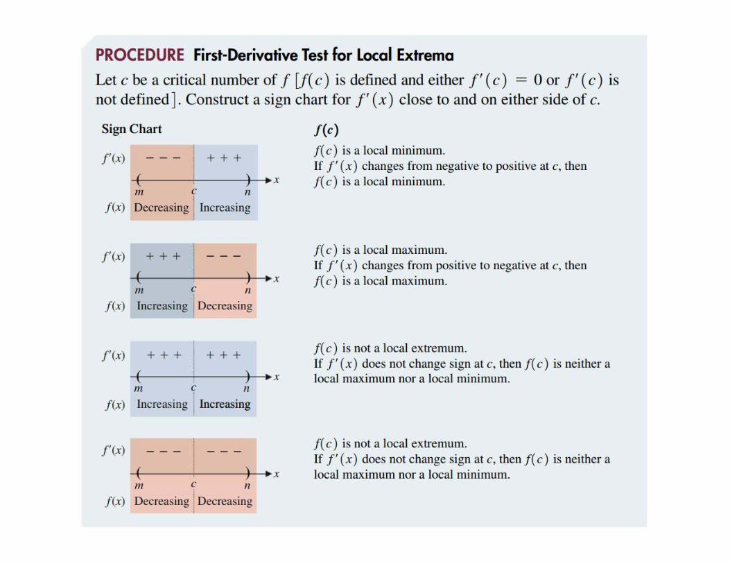
Furthermore, notice that not all critical numbers for 𝑓(𝑥) correspond to points on the graph that

have a local max or min. The key criterion is that for a critical number 𝑥 = 𝑐 to be the location of a

local max or min, 𝑓(𝑥) must change from increasing to decreasing, or from decreasing to

increasing, at 𝑥 = 𝑐. That is the essence of the First-Derivative Test.

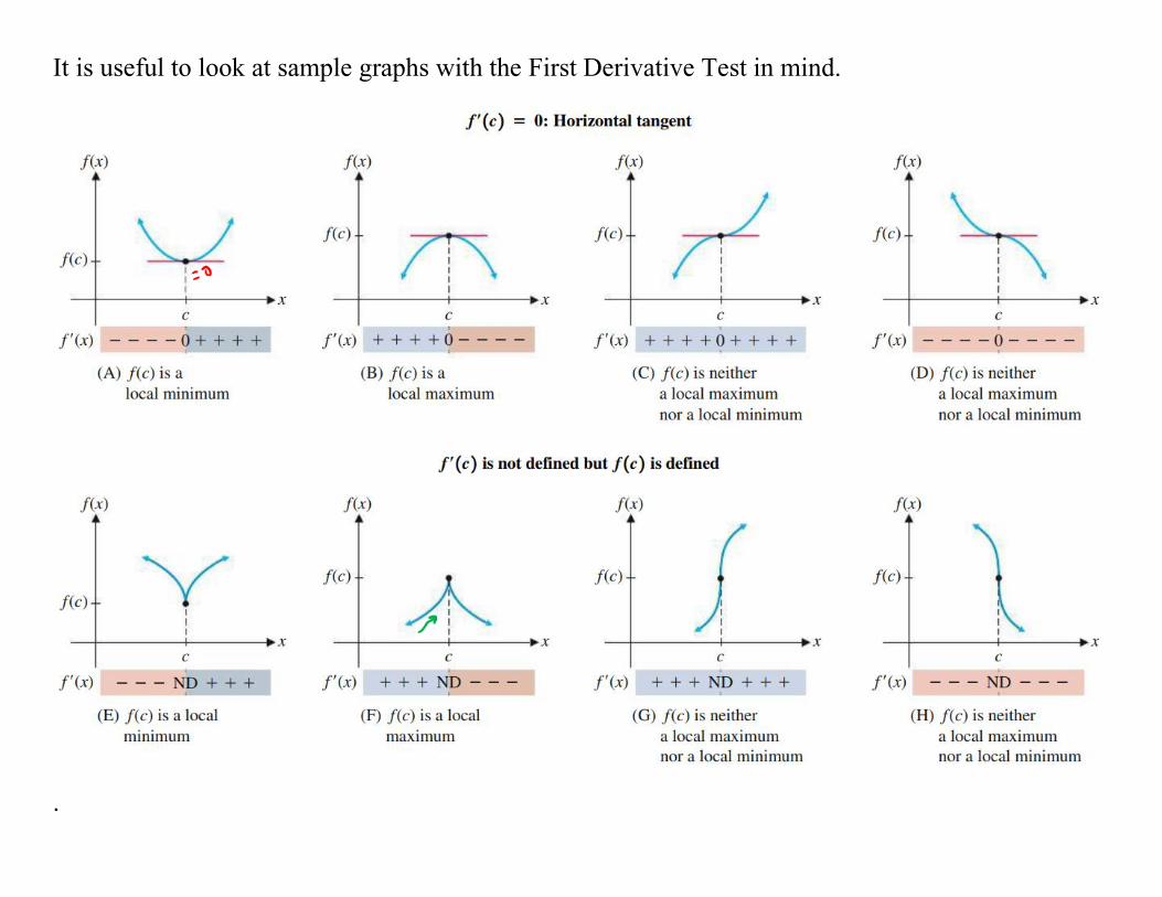
It is useful to look at sample graphs with the First Derivative Test in mind.

.

[Example 1] (Similar to 4.1#17) A function 𝑓(𝑥) is continuous on the interval (−∞,∞).

The sign chart for 𝑓′(𝑥) is shown below.

Find the 𝑥 coordinates of all local extrema of 𝑓(𝑥).

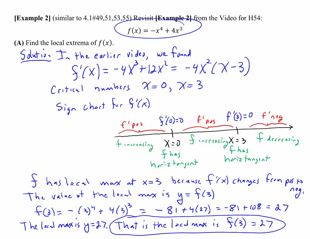
[Example 2] (similar to 4.1#49,51,53,55) Revisit [Example 2] from the Video for H54:

𝑓(𝑥) = −𝑥4+ 4𝑥

3

(A) Find the local extrema of 𝑓(𝑥).

(B) Illustrate on the given graph of 𝑓(𝑥).

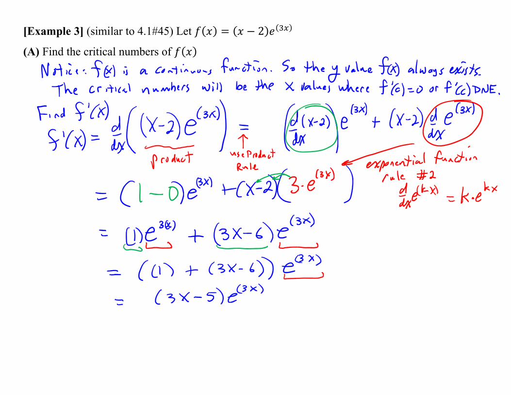
[Example 3] (similar to 4.1#45) Let 𝑓(𝑥) = (𝑥 − 2)𝑒(3𝑥)

(A) Find the critical numbers of 𝑓(𝑥)

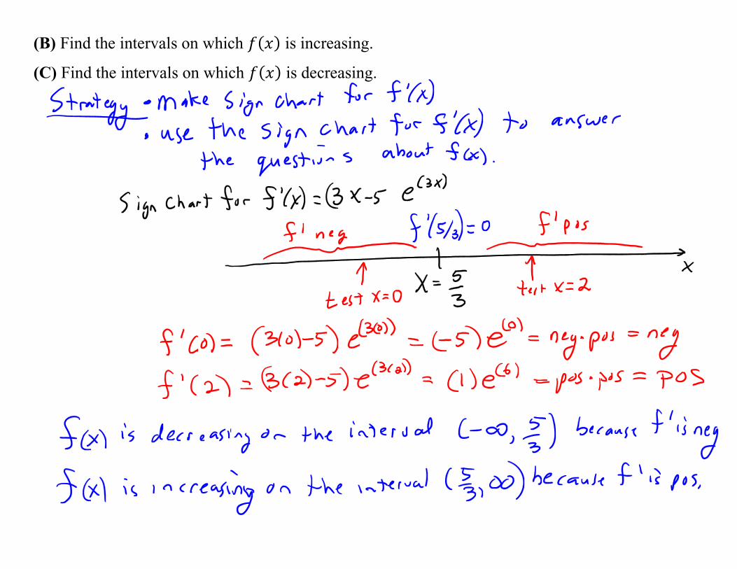
(B) Find the intervals on which 𝑓(𝑥) is increasing.

(C) Find the intervals on which 𝑓(𝑥) is decreasing.

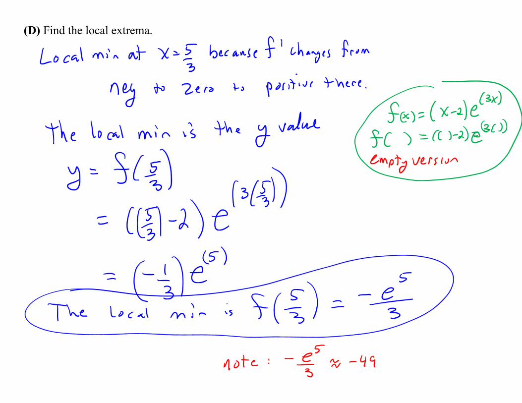
(D) Find the local extrema.

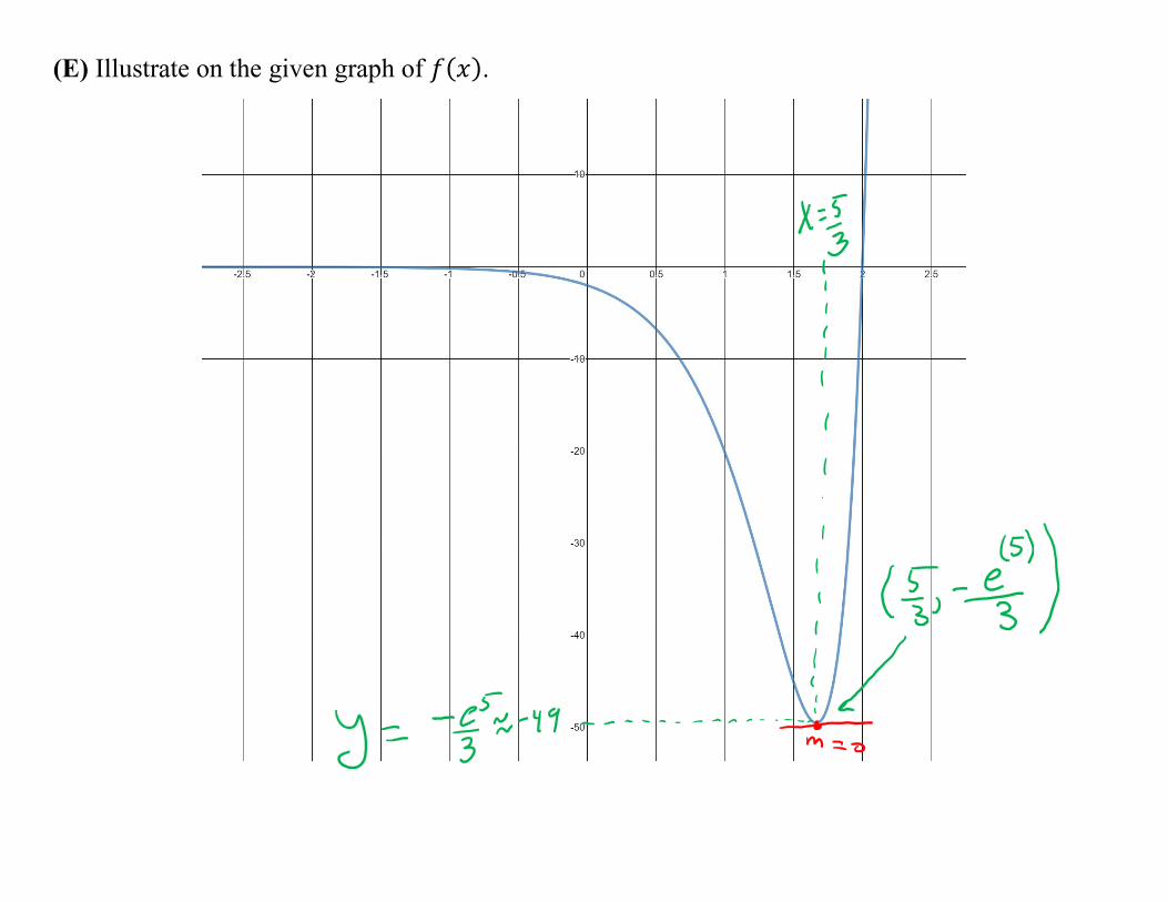
(E) Illustrate on the given graph of 𝑓(𝑥).

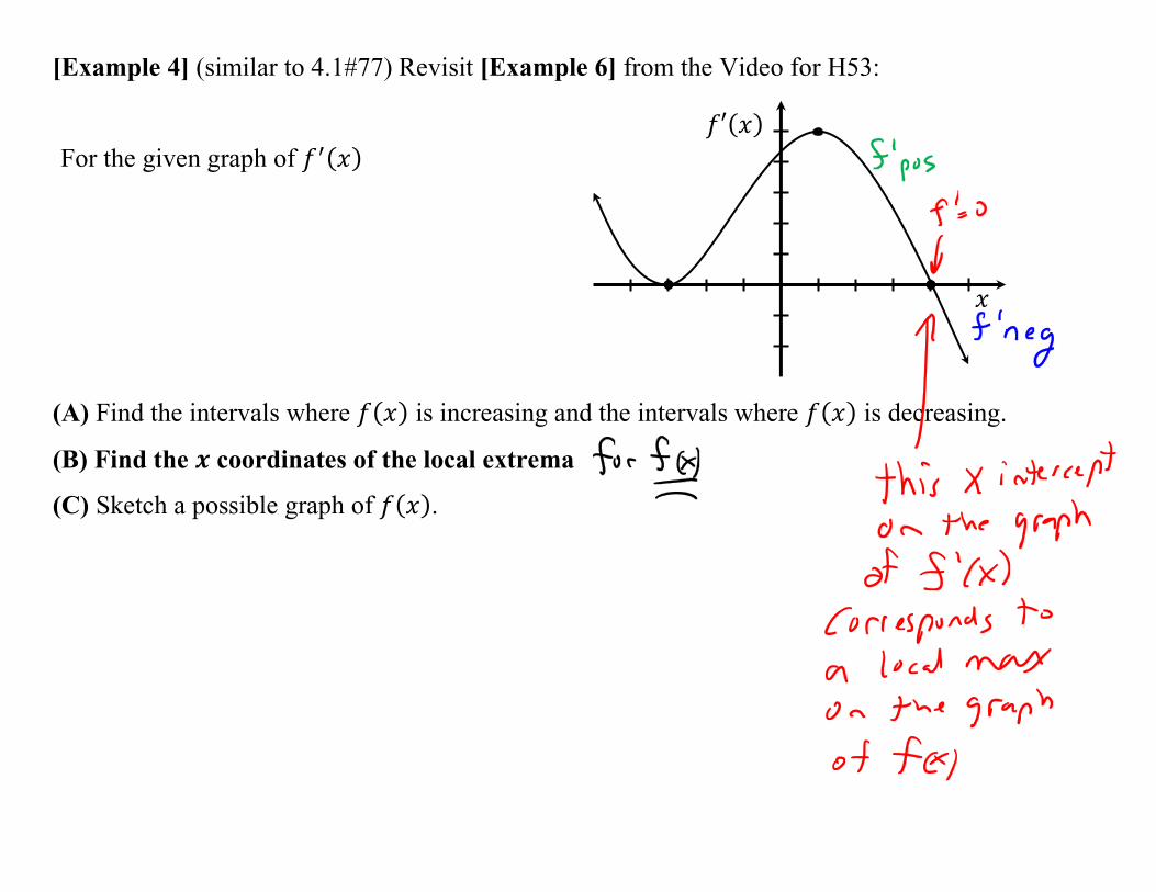
[Example 4] (similar to 4.1#77) Revisit [Example 6] from the Video for H53:

For the given graph of 𝑓′(𝑥)

(A) Find the intervals where 𝑓(𝑥) is increasing and the intervals where 𝑓(𝑥) is decreasing.

(B) Find the 𝒙 coordinates of the local extrema

(C) Sketch a possible graph of 𝑓(𝑥).

𝑥

𝑓′(𝑥)

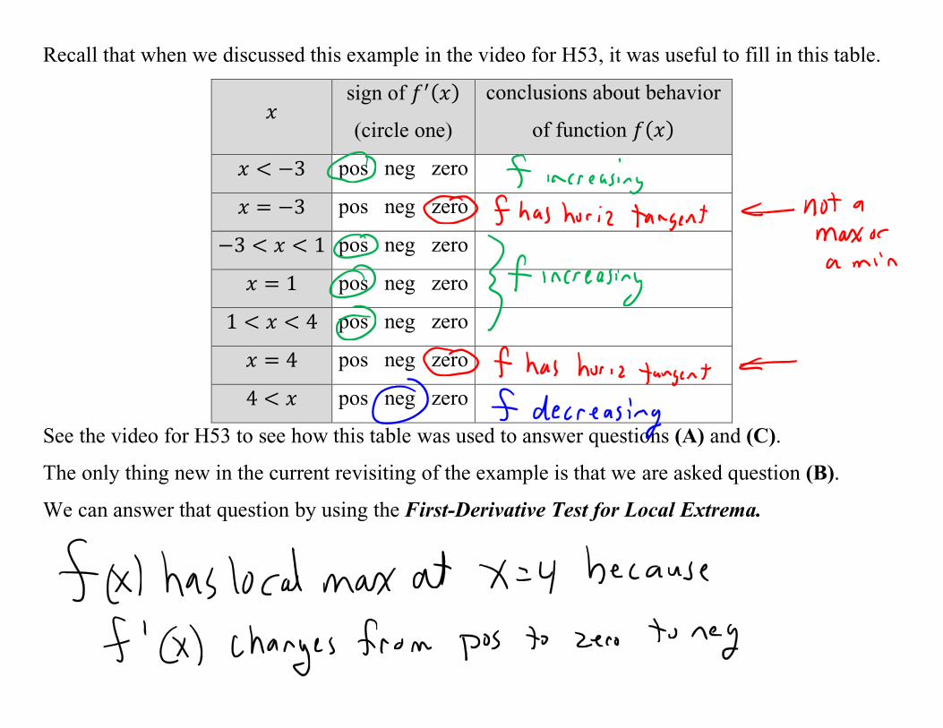
Recall that when we discussed this example in the video for H53, it was useful to fill in this table.

𝑥 sign of 𝑓′(𝑥)

(circle one)

conclusions about behavior

of function 𝑓(𝑥)

𝑥 < −3 pos neg zero

𝑥 = −3 pos neg zero

−3 < 𝑥 < 1 pos neg zero

𝑥 = 1 pos neg zero

1 < 𝑥 < 4 pos neg zero

𝑥 = 4 pos neg zero

4 < 𝑥 pos neg zero

See the video for H53 to see how this table was used to answer questions (A) and (C).

The only thing new in the current revisiting of the example is that we are asked question (B).

We can answer that question by using the First-Derivative Test for Local Extrema.

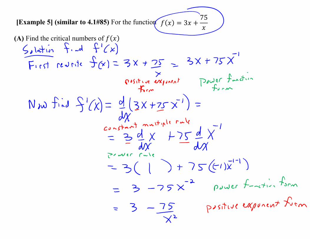
[Example 5] (similar to 4.1#85) For the function 𝑓(𝑥) = 3𝑥 +75

𝑥

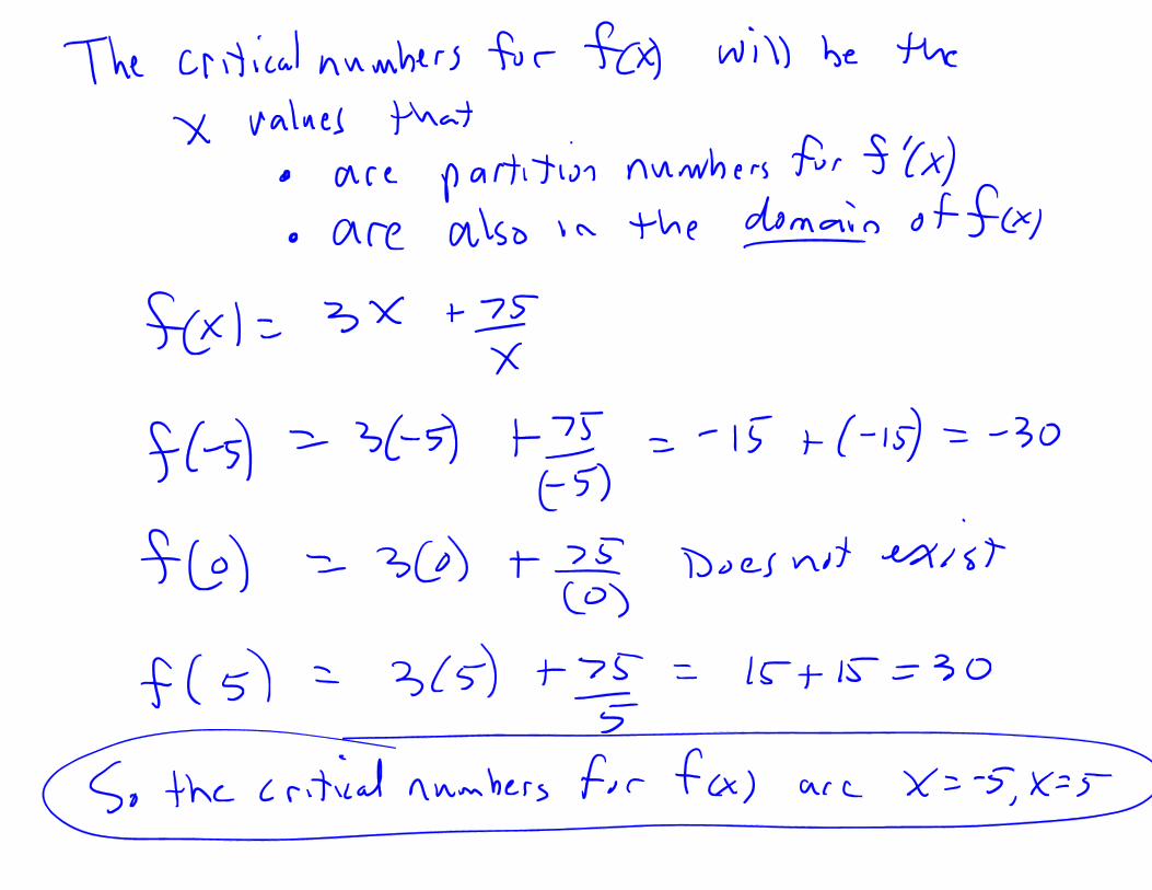
(A) Find the critical numbers of 𝑓(𝑥)

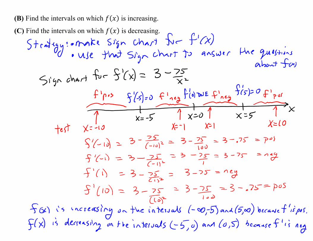
(B) Find the intervals on which 𝑓(𝑥) is increasing.

(C) Find the intervals on which 𝑓(𝑥) is decreasing.

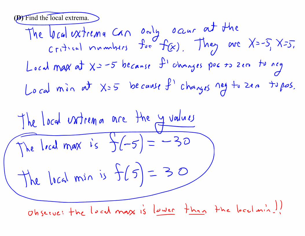
(D) Find the local extrema.

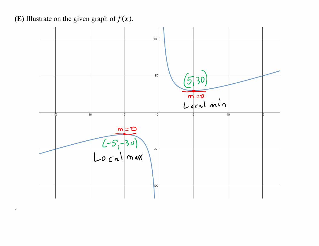
(E) Illustrate on the given graph of 𝑓(𝑥).

.

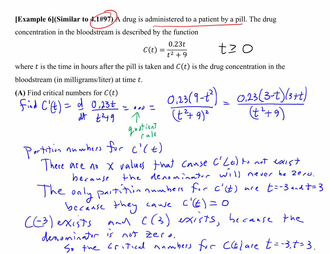
[Example 6](Similar to 4.1#97) A drug is administered to a patient by a pill. The drug

concentration in the bloodstream is described by the function

𝐶(𝑡) =0.23𝑡

𝑡2 + 9

where 𝑡 is the time in hours after the pill is taken and 𝐶(𝑡) is the drug concentration in the

bloodstream (in milligrams/liter) at time 𝑡.

(A) Find critical numbers for 𝐶(𝑡)

(B) Find intervals where 𝐶(𝑡) is increasing.

(C) Find intervals where 𝐶(𝑡) is decreasing.

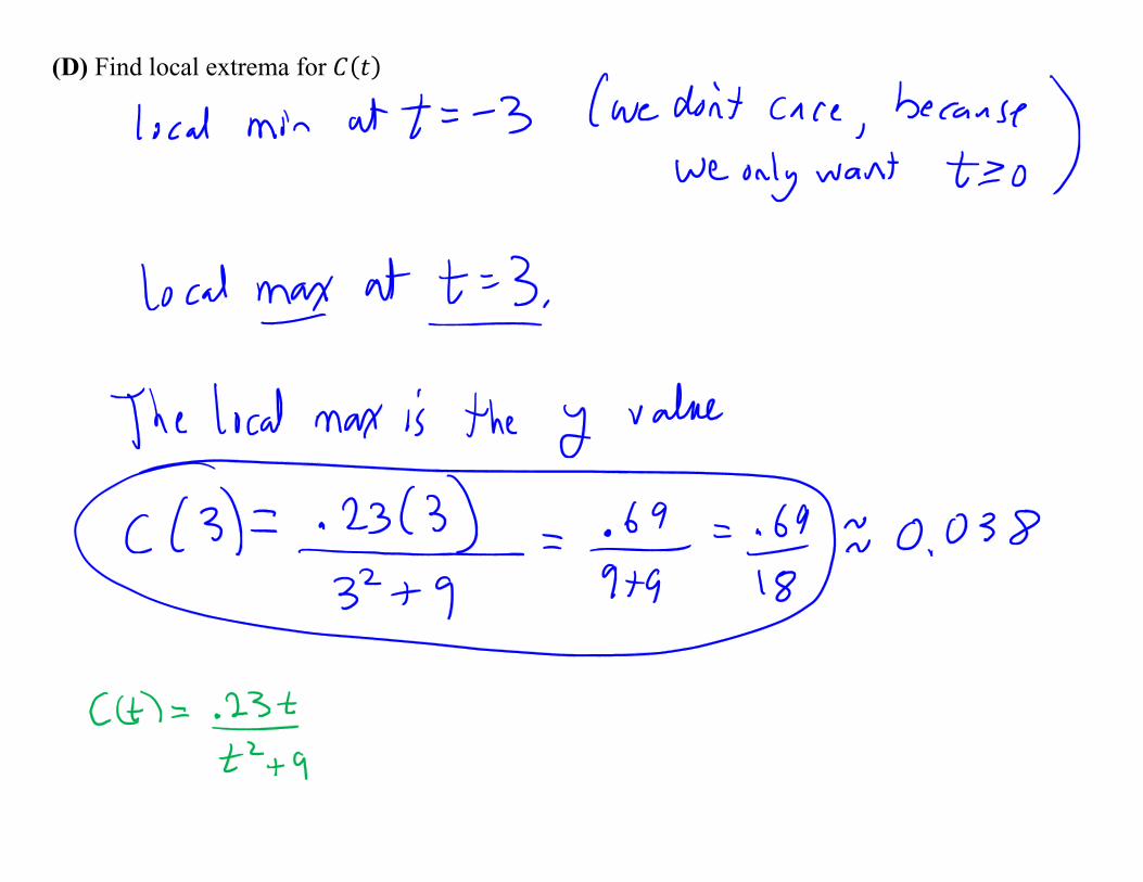
(D) Find local extrema for 𝐶(𝑡)

(E) Illustrate the results using the given graph of 𝐶(𝑡)

.