style over substance? advertising, innovation, and
TRANSCRIPT

Style Over Substance?Advertising, Innovation, and Endogenous Market Structure∗
Laurent Cavenaile
University of Toronto
Murat Alp Celik
University of Toronto
Pau Roldan-Blanco
Bank of Spain
Xu Tian
University of Toronto
March 22, 2021
Abstract
Firms use both innovation and advertising to increase their profits, markups, andmarket shares. While they serve the same purpose from the firms’ perspective, theirbroader implications vary substantially. In this paper, we study the interaction betweenthese two intangible inputs and analyze the implications for competition, industry dy-namics, economic growth, and social welfare. To this end, we develop an oligopolisticgeneral-equilibrium growth model with firm heterogeneity in which market structure isendogenous, and firms’ production, innovation, and advertising decisions strategicallyinteract. We estimate the model to fit the non-linear relationship between innovation,advertising, and competition observed in the data. We find that advertising has signifi-cant macroeconomic effects: it improves static allocative efficiency through reducingmisallocation, but it also depresses economic growth through a substitution effect withR&D. On the net, advertising is found to be welfare-improving. It is responsible for onethird of the observed average net markup, and a quarter of its dispersion. We next studythe optimal linear taxation/subsidization of advertising. We find that the optimal tax isquite high, yet finite, which serves to simultaneously increase dynamic efficiency andraise revenue, while still maintaining most of the benefits of advertising in the form ofreduced misallocation, without the excessive spending due to the advertising rat race.
Keywords: innovation, advertising, markups, growth, industry dynamics, misallocation,business dynamism.
JEL Classification: E20, L10, M30, O30, 040.
∗Contact Information: Laurent Cavenaile, 105 St. George Street, University of Toronto, Toronto, Ontario,M5S 3E6. Email: [email protected]; Murat Alp Celik, 229 Max Gluskin House, 150 St. GeorgeStreet, University of Toronto, Toronto, Ontario, M5S 3G7. Email: [email protected]; Pau Roldan-Blanco,Calle Alcalá 48, 28014, Madrid. Email: [email protected]; Xu Tian, 204 Max Gluskin House, 150 St. GeorgeStreet, University of Toronto, Toronto, Ontario, M5S 3G7. Email: [email protected]. The views expressedin this paper are those of the authors and do not necessarily coincide with those of the Banco de España orthe Eurosystem. Celik gratefully acknowledges financial support from SSHRC Insight Development Grant(503178).

1 Introduction
Firms that compete against their peers have several ways to improve their profits,
markups, and market shares. Innovation – spending resources on research and development
(R&D) to come up with new products or more efficient technologies – is a well-studied one,
which is also considered to be the engine of growth in developed economies. However,
advertising is another activity through which firms can achieve the same desired outcomes,
albeit without contributing to long-run productivity growth. On the contrary, firms might
spend exorbitant amounts in advertising in response to the advertising of their competitors,
leading to an inefficient “rat race” equilibrium with excessive spending. Since both activities
serve the same purpose, firms’ decisions to innovate and to advertise inexorably interact,
within the firm itself, as well as across all the firms in the same industry.
In practice, firms devote significant amounts of resources into both innovation and
advertising. Since 1980, R&D accounts for 2.44% of the U.S. GDP, whereas advertising
alone represents 2.20%.1 In other words, as a society, we spend as much on developing new
products and technologies (“substance”) as simply marketing them (“style”). For instance,
Procter & Gamble Company has spent 10.8% of its revenue on advertising between 2007 and
2016, which is quadruple the amount it spent on R&D (2.6%). For Unilever, the numbers
were 13.3% and 2.0%, respectively. Two natural questions to ask are (1) whether the heavy
spending in advertising is socially efficient, and (2) if the firms would reallocate resources
from advertising to R&D were they given incentives to do so. Answering these questions
and deriving their policy implications require a unified framework.
In this paper, we present a new model of firm and industry dynamics which can, in a
single framework, study the role of innovation and advertising for market concentration,
markups, and productivity growth, offering a realistic representation of how these two
forms of intangible inputs interact and relate to competition at the aggregate level. In the
model, the market structure of the economy is endogenous: the within-industry composition
between small and large firms, as well as the number of large firms within each industry, is
an equilibrium outcome. Market structure is shaped, in turn, by the production, innovation,
and advertising decisions of large firms, which determine their market share within the
industry and the markups they charge to final consumers. This is because large firms
behave strategically, internalizing the effects of their decisions on the industry’s aggregate
expenditures. Small firms, by contrast, are atomistic, charge zero markups, and make
no advertising decisions, but can innovate to come up with a breakthrough innovation
1The figures for advertising do not include in-house firm expenses related to sales, which would increasethe fraction of resources devoted to marketing further.
1

and gain access to the group of large firms. This rich yet tractable setting allows us to
tackle relevant policy questions. On the one hand, our quantitative model allows us to
study the role of the interaction between innovation and advertising for static allocative
efficiency, and to conduct policy counterfactuals to understand the role of intangibles for
static (physical-input) misallocation. On the other hand, the model allows us to study the
dynamic consequences of the innovation-advertising interaction for economic growth and
industry dynamics. Static and dynamic considerations, as well as within- and between-
industry dynamics, all matter for social welfare. Therefore, the model offers a broad
set of endogenously-generated responses, allowing us to analyze optimal policy from an
all-encompassing standpoint.
In the model, R&D and advertising are modeled as intangible expenditures which
can shift demand toward the firm’s product. R&D is modeled following the tradition of
the Schumpeterian creative-destruction literature. We model advertising to be akin to
a zero-sum game: advertising expenditures increase the perceived quality of the firm’s
product, making it more appealing to consumers, but also lower the perceived quality of
all the competitors’ products. Large firms, which are heterogeneous in productivity, choose
advertising optimally to maximize static profits, taking into account the effects on their
own market share. Because large firms behave strategically, they must also internalize
the effect of their production and advertising decisions on industry-level expenditures. In
equilibrium, the differential use of advertising across firm size can magnify productivity
differences and have quantitatively significant implications for within-industry markup
dispersion and, as a consequence, allocative efficiency. Moreover, because in equilibrium
firms are heterogeneous in their use of advertising, there is a dynamic interplay between
advertising and R&D decisions, which at the aggregate level has an impact on the rate of
economic growth and social welfare.
To study these questions quantitatively, we estimate the model by simulated method of
moments to fit key empirical patterns relating advertising and innovation to competition.
As our quantitative analysis focuses on the aggregate welfare implications stemming from
both micro- and macro-level effects, in the estimation stage, we make sure that the model
fits the data well at different levels of aggregation, namely between firms within industries,
across industries, and in terms of macroeconomic aggregates. Importantly, our model can
reproduce the empirically-observed non-linear relationship between innovation, advertising,
and market share within industries, which helps us discipline our counterfactual experiments.
In the data, both innovation and advertising expenditures exhibit an inverted-U shaped
relationship with respect to a firm’s relative sales. The estimated model matches the linear
term and top point of both of these hump-shaped curves. Using the estimated set of
2

parameters, we find that markups, R&D expenditures, and advertising expenditures are all
positively correlated at the firm level, consistent with the idea that firms use both types of
intangibles to increase their profits and exert greater market power.
Next, we conduct a series of counterfactual experiments to understand the interplay
between R&D and advertising at various levels of aggregation, and ultimately to assess the
effects of advertising on misallocation, growth, and welfare. In the first experiment, we
compare the estimated model with a counterfactual economy in which advertising is shut
down completely (e.g. it is infinitely costly for firms). We find that shutting down advertising
increases firm-level investment in R&D, both by large firms as well as small firms, thereby
increasing both aggregate innovation and the rate of economic growth. Thus, advertising
and R&D are substitutes, consistent with the empirical findings in Cavenaile and Roldan-
Blanco (2021). Shutting down advertising also affects markups and allocative efficiency
through changes in the competitive structure of industries. We find that the average net
markup decreases by one third of its value relative to the baseline economy, as large firms
cease to use advertising as a tool to shift demand and profits toward their products. This
implies that advertising is responsible for a significant fraction of the empirically-observed
average markup. Because there is less product differentiation, markups are lower and the
labor share higher in an economy without advertising. However, in spite of these effects, we
find that advertising in fact improves allocative efficiency because of its reallocative effects.
While increasing markups, advertising simultaneously reallocates physical inputs away from
the less efficient firms, and towards the more efficient industry leaders; as well as amplify
the relative perceived quality of the more abundant and cheaper to produce varieties. While
markups themselves lower efficiency, the latter two effects quantitatively dominate.
To assess the relative quantitative importance for social welfare of the various static and
dynamic channels identified above, we show that the change in welfare can be decomposed
into changes in relative wages, in the relative industry output of large firms, in the con-
sumption share of GDP, and in the rate of economic growth. We find substantial differences
between static and dynamic welfare changes. Statically (i.e. without adjustments in the firm
productivity distribution), shutting down advertising results in a welfare loss of 2.83% in
consumption-equivalent terms, mostly coming from the aforementioned losses in allocative
efficiency. Taking dynamic aspects into consideration by allowing the distribution to adjust
undoes some of these losses in the long run, as shutting down advertising also raises the
consumption share of GDP and increases the rate of economic growth through the substitu-
tion effect between R&D and advertising. All in all, the combination of the various static
and dynamic conflicting forces results in a welfare loss of 0.54% in consumption-equivalent
terms from shutting down advertising.
3
In light of these results, in the last part of the paper, we ask how the design of policy
instruments should view these welfare results. Although we conclude that shutting down
advertising would reduce dynamic efficiency, we find that advertising should be taxed, rather
than subsidized, and at the considerably high rate of 64.6%. How does one reconcile the two
findings? The answer lies in understanding how taxation differs from a complete shutdown.
Higher taxes on advertising expenses discourage the firms from investing resources in
advertising, resulting in both direct gains in the consumption-to-output ratio, and indirect
gains from improved incentives for innovation and growth. However, the taxes do not cause
as large a drop in static allocative efficiency as a complete shutdown would: while the
overall spending on advertising declines, more productive superstars still continue to spend
more on advertising than less productive ones. Therefore, the positive effects of advertising
due to the more efficient reallocation of resources are still present even under high tax
rates. In other words, the taxes reduce the excessive spending on advertising due to the
“rat race” between the superstars, while still largely preserving the relative market shares in
equilibrium. This makes advertising a perfect candidate for taxation to raise revenues while
simultaneously increasing dynamic efficiency.
Literature Review Our paper is primarily related to a literature that studies the implica-
tions of intangible investments, primarily in the form of advertising and customer capital,
for firm, industry and macroeconomic dynamics (e.g. Gourio and Rudanko (2014), Molinari
and Turino (2017), Perla (2019), Dinlersoz and Yorukoglu (2012), and Greenwood, Ma, and
Yorukoglu (2020)). The literature has investigated, for instance, how intangibles may be
behind several trends related to business dynamism, market concentration and markups (e.g.
Aghion, Bergeaud, Boppart, Klenow, and Li (2019), DeRidder (2020) and Weiss (2019)), or
how they may affect markup cyclicality (Roldan-Blanco and Gilbukh (2021)), firm’s market
value and risk (Belo, Lin, and Vitorino (2014)), the transmission channels of monetary policy
(Morlacco and Zeke (2020)), and the behavior of exporters and international prices (Drozd
and Nosal (2012), Fitzgerald, Haller, and Yedid-Levi (2017)). Our model is most closely
related to endogenous growth models with advertising such as Rachel (2021) and, more
particularly, Cavenaile and Roldan-Blanco (2021). Rachel (2021) studies how the provision
of free leisure-enhancing technologies that firms can use to build their brand equity (e.g.
through advertising) can explain the observed decline in hours workers and affect negatively
innovation and TFP growth.2 In a model with monopolistic competition, Cavenaile and
2Greenwood, Ma, and Yorukoglu (2020) also consider the implication of advertising embedded in freemedia on hours worked and welfare but do not study its effect on economic growth. They find that theexpansion of free media arising from the advent of digital advertising is welfare improving. However, someadvertising is wasteful and a tax on advertising might be required to correct for this source of inefficiency.
4

Roldan-Blanco (2021) show that there exists an interaction between R&D and advertising
investment at the firm level which shapes the firm size distribution, firm dynamics, and
long-run economic growth. In the present paper, we explore how this interaction further
affects market concentration, markups, productivity growth, and welfare. Moreover, as in
Cavenaile and Roldan-Blanco (2021), we find that advertising and R&D are substitutes,
even though the two theoretical frameworks are different.
Our paper also contributes to the growing literature studying heterogeneous-firm
economies with markup distortions (e.g. Edmond, Midrigan, and Xu (2018), Burstein,
Carvalho, and Grassi (2020), Baqaee and Farhi (2020)). Within this literature, we are most
closely related to models of endogenous growth with variable markups, e.g. Akcigit and
Ates (2019a,b), Peters and Walsh (2019), Liu, Mian, and Sufi (2019), Aghion, Bergeaud,
Boppart, Klenow, and Li (2019), Peters (2020) and, particularly, Cavenaile, Celik, and Tian
(2020). In our model, as in models of oligopolistic competition in the spirit of Atkeson and
Burstein (2008), firm-level markups are increasing in the market share of firms. However,
as in Cavenaile, Celik, and Tian (2020), market structure is endogenous. In addition, there
is an interplay between market shares and firms’ innovation decisions. To this framework,
we add advertising decisions at the firm level, which in equilibrium directly affect market
shares and markups as well as R&D decisions.
More generally, our paper contributes to a long tradition of modeling advertising in
economics (e.g. Dorfman and Steiner (1954), Butters (1977), Becker and Murphy (1993),
Benhabib and Bisin (2002)).3 In the literature, advertising mostly acts as a demand shifter
by affecting demand preferences. Similarly, we model advertising as a technology that shifts
consumer preferences for certain goods to the detriment of competitors’ products, which in
equilibrium means that firms can use advertising expenditures to shift demand toward their
own goods, thereby affecting their market share and the markups they set. To draw this
connection between firm-level advertising and market structure, we rely on observations
from various papers relating market concentration to intangible investments. Crouzet and
Eberly (2019) argue that the increase in intangible capital investments driven by large firms
may be behind the rise in industry concentration in the last two decades, while De Loecker,
Eeckhout, and Unger (2020) find a positive firm-level relation between markups and both
R&D and advertising expenditures for publicly-traded firms. In our model, these types of
relationships emerge endogenously, and help explain the macroeconomic implications of
R&D and advertising on growth and welfare.
3Bagwell (2007) provides a comprehensive survey of the advertising literature in economics.
5

Outline The remainder of the paper is organized as follows: Section 2 presents our
model of endogenous markups, innovation, advertising and market structure. Section 3
discusses the estimation of the model and main quantitative features of the equilibrium.
Section 4 conducts a number of counterfactual experiments using the estimated parameters,
describing the macroeconomic effects of advertising on the composition of industries, the
level and dispersion of markups, the rate of economic growth, and social welfare (Section
4.1). Moreover, we analyze the optimal taxation of advertising within the context of the
estimated model (Section 4.2). Section 5 offers some concluding remarks.
2 Model
2.1 Environment
In this section, we develop an oligopolistic general-equilibrium growth model with firm
heterogeneity in which market structure is endogenous, and firms’ production, innovation,
and advertising decisions strategically interact. This new model of firm and industry
dynamics can, in a single framework, study the role of innovation and advertising for market
concentration, markups, and productivity growth, offering a realistic representation of how
these two forms of intangible inputs interact and relate to competition at the aggregate
level.
Preferences Time is continuous, infinite, and indexed by t ∈ R+. The economy is
populated by an infinitely-lived representative consumer who maximizes lifetime utility:
W =∫ +∞
0e−ρt ln(Ct) dt (1)
where ρ > 0 is the time discount rate, and Ct is consumption of the final good at time t. The
price of the final good is normalized to one. The household is endowed with one unit of
time every instant, supplied inelastically to the producers of the economy in return for a
wage wt which clears the labor market. The household owns all the firms in the economy
and carries a stock of wealth At each period, equal to the total value of corporate assets.
The budget constraint satisfies At = rtAt + wt − Ct, where rt is the rate of return on assets.
The usual no-Ponzi-scheme condition holds.
6

Final Good Production The final good Yt is produced by a representative firm using
inputs from a measure one of industries, with technology:
Yt = exp(∫ 1
0ln(yjt)
dj)
(2)
where yjt is production of industry j at time t.
Industry Production Each industry j is populated by an endogenous number of superstar
firms, Njt ∈ {1, ..., N}, each producing a differentiated variety, as well as by a competitive
fringe composed of a mass mjt of small firms producing a homogeneous good. Industry j’soutput at time t is given by:
yjt =
(y
γ−1γ
cjt + yγ−1
γ
sjt
) γγ−1
(3)
where ycjt denotes the output of the fringe, ysjt denotes the output of superstars, and
γ ≥ 1 is the elasticity of substitution between the two. Fringe firms produce a homogenous
product, so:
ycjt =∫
Fjt
yckjt dk (4)
where Fjt is the endogenous set of small firms in the fringe in industry j at time t. Given that
there is a continuum of small firms and their products are homogeneous, each small firm
in the competitive fringe is a price taker. By contrast, superstar firms behave strategically,
competing in quantities in a static Cournot game. Total production by superstars of industry
j at time t is given by:
ysjt =
Njt
∑i=1
ωijtyη−1
η
ijt
η
η−1
(5)
where η > 1 is the elasticity of substitution between varieties, holding η > γ. Each variety
has quality ωijt, defined by:
ωijt =1 + ωijt
1Njt
∑Njtk=1(1 + ωkjt)
(6)
In this expression, ωijt is a quality shifter which is affected by the superstar firm’s
7

advertising decisions, as described below. The effective quality of a product, ωijt, is the
ratio of this quality shifter to the average shifter among the superstars within the industry.
Intuitively, we model advertising as a technology which allows firms to shift the perceived
quality of their own product. Moreover, all else equal, if a firm chooses to increase its
advertising efforts, it will increase the perceived quality of its own product while decreasing
that of every other product. In this sense, advertising is akin to a zero-sum game, in which a
firm’s advertising efforts are directly detrimental to other firms’ product qualities, but so
that if all superstars were to choose the same ω level, then all varieties would have the same
baseline quality. This baseline quality coincides with the quality of the product of the fringe,
which is normalized to one.
Firms’ Production Technology In each industry, superstar firms and small firms in the
fringe produce their variety using a linear production technology in labor:
yijt = qijtlijt and yckjt = qcjtlckjt (7)
where lijt and lckjt denote the labor input, qijt is the productivity of superstar firm i in
industry j at time t, and qcjt is the productivity of a fringe firm. Each small firm from the
fringe is assumed to have the same productivity within an industry. Superstar firms, by
contrast, are heterogeneous in their level of productivity, which can be built over time
through R&D and innovation.
R&D and Innovation Each superstar can perform R&D to improve the productivity of its
variety. To generate a Poisson rate zijt of success in R&D, firm i must pay:
Rijt = χzφijtYt (8)
units of the final good, where χ > 0 and φ > 1 are parameters. A successful innovator is
able to advance its productivity by a factor (1 + λ), where λ > 0. As we shall see shortly,
industry-level outcomes in this model depend on the relative levels of productivity between
superstar firms, which can be summarized by an integer nkijt ∈ {−n,−n + 1, ..., n− 1, n}
holding:qijt
qkjt= (1 + λ)
nkijt (9)
In words, nkijt is the number of productivity steps by which firm i in industry j is ahead
(if nkijt > 0), behind (if nk
ijt < 0) or neck-to-neck (if nkijt = 0) with respect to firm k 6= i at
time t. The parameter n ≥ 1 is the maximum number of steps between any two superstar
8

firms within an industry. For the competitive fringe, we assume that the relative productivity
of small firms with respect to the leader is a constant, denoted by the parameter ζ =qcjt
qleaderjt
,
where qleaderjt ≡ maxk=1,...,Njt{qkjt}.
Advertising Each superstar firm can spend resources on advertising its product to affect
the quality shifter ωijt. In order to achieve a perceived quality ωijt, firm i of industry j must
spend
Aijt = χaωφaijtYt (10)
units of the final good, where χa > 0 and φa > 1 are parameters.
Entry and Exit of Superstar Firms At any time t, each small firm k in the competitive
fringe can generate a Poisson arrival rate Xkjt and enter into the pool of superstar firms, as
long as Njt < N for some N set exogenously. The associated R&D cost is given by
Rekjt = νXε
kjtYt. (11)
with ν > 0 and ε > 1. As small firms are all homogeneous within the same industry, their
level of innovation is identical in equilibrium. This allows us to write an industry-level
Poisson rate of innovation Xjt =∫
Xkjtdk = mjtXkjt. Similarly, the R&D expenditures of
small firms at the industry level equal Rejt = mjtRe
kjt.
Upon successful entry (provided Njt < N), the entrant is assumed to enter as the smallest
superstar firm within the industry and thus becomes a superstar firm with productivity level
n steps behind the leader. In this case, the number of superstar firms Njt increases by one.
On the other hand, a superstar firm endogenously loses its superstar status when it falls
more than n steps below the industry leader. In that case, the number Njt decreases by one.
Entry and Exit of Small Firms Finally, there is entry into and exit out of the competitive
fringe. We assume an exogenous exit rate of small firms equal to τ. For entry, we assume
there is a measure one of entrepreneurs who pay a cost ψe2t Yt to generate a Poisson rate
et of starting a new small firm, where ψ > 0. New firms are randomly allocated to the
competitive fringe of an industry, implying mjt = mt for all industries j. We further assume
that successful entrepreneurs sell their firm on a competitive market at its full value and
remain in the set of entrepreneurs, which keeps the mass of entrepreneurs unchanged.
9
2.2 Equilibrium
Household’s Problem Household utility maximization delivers the standard Euler equa-
tion:
Ct
Ct= rt − ρ. (12)
Final Good Producers The final good is produced competitively. The representative final
good producer chooses the quantity of each variety in each industry to achieve a given
level of output which minimizes total production costs. This leads to the following demand
functions for superstar and fringe firms, respectively:
yijt = ωηijt
(pijt
psjt
)−η (psjt
pjt
)−γ1
pjtYt (13)
ycjt =
(pcjt
pjt
)−γ1
pjtYt (14)
where pijt is the price of the variety produced by superstar i in industry j at time t, and pcjt is
the price of the homogenous product of the competitive fringe of that industry. Additionally,
we have defined psjt ≡(
∑Njti=1 ω
ηijt p1−η
ijt
) 11−η
as the ideal price index among the different
varieties of the superstars and pjt ≡(
p1−γsjt + p1−γ
cjt
) 11−γ as the ideal price index of the
industry. The allocation of expenditures among superstar firms of the same industry is
determined by perceived product qualities ωijt as well as the price of each firm’s product
relative to other superstars in its industry,pijtpsjt
, with price-elasticity η. In particular, the
relative output between any two superstars i and k of the same industry is:
yijt
ykjt=
(ωkjt
ωijt
pijt
pkjt
)−η
(15)
This makes it apparent that firms can use advertising to shift demand toward their
products and thereby increase profits at the expense of their direct competitors. The
allocation of expenditure between superstars and small firms within the same industry is
determined by the relative price indexpsjtpjt
, with price-elasticity γ. In particular, the relative
output between a superstar and a fringe firm belonging to the same industry is:
yijt
ycjt= ω
ηijt
(pijt
psjt
)−η (psjt
pcjt
)−γ
(16)
10

Finally, the allocation of expenditure across industries is determined by the relative price
of the industry to the price of the final good, 1pjt
. Within-industry expenditures hold:
psjtysjt =
Njt
∑i=1
pijtyijt and pjtyjt = psjtysjt + pcjtycjt (17)
among superstars alone (excluding the fringe), and including superstars and fringe, respec-
tively.
Market Shares and Markups Each superstar firm makes output (yijt) and advertising
(ωijt) choices to maximize profits:
maxyijt,ωijt
{pijtyijt − wtlijt − χaω
φaijtYt
}(18)
subject to equations (13)-(14) and yijt = qijtlijt. We assume that superstar firms within the
same industry compete à la Cournot, so they internalize how their output choices affect
the aggregate output within their industry. In equilibrium, each superstar firm i sets a
price markup over the marginal cost of production, so that the price is pijt = Mijtwtqijt
. The
equilibrium markup is given by:
Mijt =
[(η − 1
η
)−(
γ− 1γ
)σijt −
(η − γ
ηγ
)σijt
]−1
(19)
In this formula, we have defined:
σijt ≡pijtyijt
pjtyjtand σijt ≡
pijtyijt
psjtysjt(20)
as, respectively, the market share of firm i among all firms (superstars and fringe) in its
industry, and the market share of the firm among the superstars only.4 Equation (19) shows
that a firm’s markup is increasing in both of these market share measures. Importantly, we
4Indeed, the numerators in Equation (20) are firm sales while, by equation (17), the denominator of σ(respectively, σ) equals the industry’s expenditures including (respectively, excluding) the fringe.
11

can write market shares in terms of relative outputs and productivities, as follows:5
σijt =
ωijt
(∑
Njtk=1 ωkjt
(ykjtyijt
) η−1η
) γ−ηγ(η−1)
(ycjtyijt
) γ−1γ
+
(∑
Njtk=1 ωkjt
(ykjtyijt
) η−1η
) η(γ−1)γ(η−1)
and σijt =ωijt
∑Njtk=1 ωkjt
(ykjtyijt
) η−1η
(21)
In combination with the demand functions derived above, this allows us to obtain the
following set of static equilibrium conditions:
(yijt
ykjt
) 1η
=qijt
qkjt
ωijt
ωkjt
Mkjt
Mijt, ∀k 6= i (22a)
yijt
ycjt=
qijt
qcjt
σijt
σcjt
1Mijt
. (22b)
where σcjt ≡ 1−∑Njtk=1 σkjt is the market share of the fringe. In words, the relative demand of
superstars is increasing in its relative productivity and relative taste shifter, and decreasing
in its relative markup. The static profits before advertising costs (πijt = pijtyijt − wtlijt) are
proportional to the product of the superstar’s market share and the Lerner index:
πijt = σijt(1−M−1ijt )Yt (23)
Advertising Choices We denote post-advertising profits by πadvijt ≡ πijt− χaω
φaijtYt. As with
output choices, a superstar firm internalizes that its advertising decisions affect industry-
level prices through their effects on the firm’s own market shares relative to other superstars
and the fringe, its markups, as well as on other firms’ market shares and markups. The
optimal level of advertising ωijt by firm i in industry j satisfies∂πijt∂ωijt
= χaφaωφa−1ijt , equating
the marginal static profit gains from advertising to the marginal cost of advertising. Using
equation (23), we can further write:
∂σijt
∂ωijt(1−M−1
ijt ) + σijt∂(1−M−1
ijt )
∂ωijt= χaφaω
φa−1ijt (24)
This equation shows that marginal profit gains from advertising, on the left-hand side,
come from two channels: effects directly through changes in the firm’s market share, and
5In fact, a simple mapping between σ and σ is σijtyγ−1
γ
sjt = σijtyγ−1
γ
jt .
12

those coming through changes in markups. Using the equilibrium conditions provided
above, Equation (24) can be further written as only a function of (ω, σ), and parameters:
σijt
1 + ωijt
∑k 6=i(1 + ωkjt)
∑Njtk=1(1 + ωkjt)
[1−(
η − γ
γ(η − 1)
)σijt −
((γ− 1)ηγ(η − 1)
)σijt
]= χaφaω
φa−1ijt (25)
This formulation of the optimality condition shows that the firm must also internalize
the advertising efforts of all of its competitors, as these affect the average product quality
and thus the demand shifter of each of the superstars.
As both markups and taste shifters are functions of market shares, and these are them-
selves functions of relative outputs, equations (22a)-(22b) comprise a system of Njt equa-
tions and Njt unknowns (the output ratios), which can be solved, for each industry j, as a
function of the set of relative productivities between firms, {nkijt}, and the total number of
superstars in the industry, Nj. Though the model does not admit closed-form solutions for
(ω, σ, M), the resulting equilibrium relationship between these variables will be discussed
within the context of the estimated set of parameters in Section 3.
Labor Market Clearing We close the static part of the equilibrium by imposing labor
market clearing. Labor input choices satisfy:
lijt =σijt
wrelt
M−1ijt and lcjt =
σcjt
wrelt
(26)
for each superstar firm i and the fringe, respectively, where wrelt ≡
wtYt
denotes the relative
wage. Imposing labor market clearing,∫ 1
0 (lcjt + ∑Njti=1 lijt) dj = 1, gives us a formula for this
relative wage:6
wrelt =
∫ 1
0
σcjt +
Njt
∑i=1
σijtM−1ijt
dj (27)
Superstar Value Function and R&D Decision As we have just seen, static production and
advertising decisions, markups, and profits within each industry only depend on the number
of superstars and the distribution of their relative productivities. Therefore, the relevant
state of a firm i in industry j is given by the vector collecting the number of productivity
steps relative to all other superstars in the industry, nijt = {nkijt}k 6=i, and the number of
6Note that the relative wage (which, in this economy, is nothing but the aggregate labor share) may beinterpreted as the inverse of the aggregate markup, the latter defined as a harmonic average of firm-levelmarkups.
13

superstars in the industry, Njt = |nijt|+ 1. Let us drop time subscripts unless otherwise
needed. A superstar firm i chooses an innovation rate zi to maximize the value of the firm
given by:
rV(ni, N) = maxzi
{πadv(ni, N)− χzφ
i Y
+ zi
[V(
ni\{nki = n}+ 1, N − |{nk
i = n}|)−V(ni, N)
]+ ∑{k:nk
i =−n}zkj
(0−V(ni, N)
)+ ∑{k:nk
i >−n}zkj
[V(
ni\{nki } ∪ {nk
i − 1}\{nli = n + nk
i }, N − |{nli = n + nk
i }|)−V(ni, N)
]
+ Xj
[V(ni ∪ {min {n, n + min(ni)}}, min(N + 1, N))−V(ni, N)
]}+ V(ni, N)
(28)
In this Hamilton-Jacobi-Bellman equation, the first line is the flow profit from sales net
of labor and advertising costs, minus the costs from R&D. The firm term on the second line
is the gain from a successful innovation, which increases the lead of the firm by one relative
to all of its competitors. Any firm n productivity steps below firm i exits the set of superstars,
which decreases the number of firms by one. The second term on this line is the change in
value due to endogenously exiting the set of superstars after a successful innovation by the
industry leader who is n steps ahead of firm i, in case any such firm exists. The third line
includes the event that any other superstar k of the industry innovates. In this case, the lead
of firm i relative to the innovating firm decreases by one. Moreover, in case the innovating
firm was leading any other firm l by n, the latter firm exits, and the number of superstars
in the industry decreases by one. The first term on the fourth line is the effect of entry on
the value of firm i, with the incoming firm starting with distance n from the industry leader.
The last term on this line is the change in value due to firm growth.
In a balanced growth path (BGP) with constant output growth g > 0, firm value holds
V(ni, N) = v(ni, N)Y for a time-invariant v, so that V(ni, N) = gv(ni, N)Y. Using equation
(12), we can write:
ρv(ni, N) = maxzi
{πadv(ni, N)
Y− χzφ
i + zi
[v(
ni\{nki = n}+ 1, N − |{nk
i = n}|)− v(ni, N)
]+ ∑{k:nk
i 6=−n}zkj
[v(
ni\{nki } ∪ {nk
i − 1}\{nli = n + nk
i }, N − |{nli = n + nk
i }|)− v(ni, N)
]
14

− ∑{k:nk
i =−n}zkjv(ni, N) + Xj
[v(ni ∪ {min {n, n + min(ni)}}, min(N + 1, N))− v(ni, N)
]}.
(29)
The optimal level of innovation is given by:
zi =
v(
ni\{nki = n}+ 1, N − |{nk
i = n}|)− v(ni, N)
χφ
1
φ−1
. (30)
Small Firm Innovation To obtain the optimal behavior of small firms and the entry into
the superstar status, we define Θ = (N,~n) as the state of the industry, where N ∈ {1, ..., N}is the number of superstars in the industry and ~n ∈ {0, ..., n}N−1 is the number of steps
followers are behind the leader (in ascending order). Further, define pli(Θ) as the arrival
rate of a leader innovation and p(Θ, Θ′) as the instantaneous flows from state Θ to Θ′. In
each industry Θ (with N(Θ) < N), each small firm in the competitive fringe chooses R&D
investment to maximize:
rVe(Θ) = maxXkj
{XkjV
({nj − n} ∪ {−n}, Nj + 1
)− τVe(Θ)− νXε
kjY
+ ∑Θ′
p(Θ, Θ′)(
Ve(Θ′)−Ve(Θ))}
+ Ve(Θ) (31)
where Ve(Θ) is the value of a small firm in industry j and nj = nkj, where k denotes a
productivity leader in industry j.7 Guessing and verifying that Ve(Θ) = ve(Θ)Y in a BGP,
the optimal innovation intensity by a small firm in industry j is then:
Xkj =
(v({nj − n} ∪ {−n}, Nj + 1
)νε
) 1ε−1
(32)
Plugging in the optimal solution, the normalized value of a small firm is:
ve(Θ) =1
ρ + τ
[(1− 1
ε
)v({nj − n} ∪ {−n}, Nj + 1)
εε−1
(νε)1
ε−1+ ∑
Θ′p(Θ, Θ′)
(ve(Θ′)− ve(Θ)
)](33)
7Note that we use∫
k=i Vek (Θ)dk = 0 in the first term, i.e., the value of the small firm is insignificant
compared to the value of the superstar firm it becomes, since it is of mass zero in the competitive fringe.
15

Entrepreneurs The expected value of a new small firm created by a successful en-
trepreneur is equal to W = ∑Θ Ve(Θ)µ(Θ), where µ(Θ) is the mass of industries of
type Θ.8 The value of being an entrepreneur (S) is:
ρS = maxe{−ψe2Y + eW} (34)
Guessing and verifying that S = sY in a BGP, we obtain that:
e =1
2ψ ∑Θ
ve(Θ)µ(Θ) (35)
which implies s = 14ψρ [∑Θ ve(Θ)µ(Θ)]2. In a stationary equilibrium, entry into the competi-
tive fringe equals exit from the competitive fringe, implying e = τm. In combination with
equation (35), we get the equilibrium measure of small firms in the economy:
m =∑Θ ve(Θ)µ(Θ)
2ψτ(36)
Equilibrium Definition An equilibrium is defined by a set of allocations {Ct, Yt, yijt, yckjt},policies {lijt, lckjt, ωijt, zijt, Xkjt, et}, prices {pijt, pcjt, wt, rt}, the number of superstars in each
industry Njt, a mass of small firms mt, a set of vectors {nijt} that denote the relative
productivity distance between firm i and every other firm in the same industry j at time t,such that, ∀t ≥ 0, j ∈ [0, 1], i ∈ {1, ..., Njt}:
(i) Given prices, final good producers maximize profit.
(ii) Given nij and Njt, superstars choose yijt and ωijt to maximize profit.
(iii) Given prices, small firms in the competitive fringe choose yckjt to maximize profit.
(iv) Superstar firms choose innovation policy zijt to maximize firm value.
(v) Small firms choose innovation policy Xkjt to maximize firm value.
(vi) Entrepreneurs choose et to maximize profit.
(vii) The real wage rate wt clears the labor market.
(viii) Aggregate consumption Ct grows at rate rt − ρ.
8We can show that the expected value of ∑Θ′ p(Θ, Θ′)(Ve(Θ′)− Ve(Θ)) in a stationary equilibrium is
equal to zero (see Proposition 1 in Appendix B.2). W is thus equal to 1− 1ε
ρ+τ (νε)1
1−ε∫ 1
0 V({nj − n} ∪ {−n}, Nj +
1)ε
ε−1 dj.
16

(ix) The aggregate resource constraint is satisfied:
Yt = Ct +∫ 1
0
Njt
∑i=1
χzφijtYt dj +
∫ 1
0
Njt
∑i=1
χaωφaijtYt dj +
∫ 1
0mtνXε
kjtYt dj + ψe2t Yt (37)
The aggregate resource constraint states that the final output is used for consumption,
incumbents’ R&D, incumbents’ advertising costs, R&D costs for small firms and entry costs.
Growth Rate Finally, the growth rate of aggregate output in this economy at time t is
given by:9
gt = −gwrel ,t + ln(1 + λ)∑Θ
plit(Θ)µt(Θ) + ∑Θ
∑Θ′
(ft(Θ′)− ft(Θ)
)pt(Θ, Θ′)µt(Θ) (38)
where gwrel ,t is the growth rate of the relative wage wrelt ≡ wt
Yt, the second term comes
from the growth rate of the industry leaders, and the third term accounts for production
reallocation as industries move between states, where we have defined:
ft(Θ) ≡ 1γ− 1
ln
1 +
Nt(Θ)
∑i=1
ωit(Θ)
(yit
yct(Θ)
) η−1η
η(γ−1)γ(η−1)
(39)
In a balanced growth path with a time-invariant distribution over Θ, we have gwrel ,t = 0and µt(Θ) = µ(Θ). Therefore, the BGP rate of economic growth is given by:
g = ln(1 + λ)∑Θ
pli(Θ)µ(Θ) (40)
In words, the growth rate of the economy is the product of the log step size of innovations
and the average leader innovation intensity across industries.
3 Quantitative Analysis
3.1 Estimation
The main focus in our counterfactual exercises in Section 4 will be to understand the
static and dynamic implications of the interaction between advertising and innovation
9See Appendix B.1 for the full derivation.
17

both within and across industries, as well as for the aggregate economy. Thus, our estima-
tion strategy requires that the model is consistent with empirical observations regarding
advertising, innovation, and markups at different levels of aggregation.
In particular, the model is estimated to replicate two within-industry inverted-U shaped
relationships observed in the data: (i) an inverted-U relationship between innovation and
firms’ market share, and (ii) an inverted-U relationship between advertising expenditures
and firms’ market share.10 Matching both of these margins helps carefully discipline the
implications for innovation, economic growth, and welfare in the various counterfactual
exercises of Section 4.
We estimate the model at an annual frequency, and set the consumer discount rate
externally to ρ = 0.04. This leaves 12 parameters to estimate: the innovation step size, λ;
the R&D cost scale parameters for superstars and small firms, (χ, ν); the corresponding
R&D cost curvature parameters, (φ, ε); the relative productivity of the competitive fringe
compared to the leader, ζ; the small firm exit rate, τ; the entry cost scale, ψ; the cost scale
and curvature parameters in the advertising cost function, (χa, φa); and two elasticities
of substitution: the elasticity among superstars’ varieties within an industry, η; and the
elasticity between the superstars’ combined output and the fringe’s combined output, γ.
Because of the non-linearities of the model, individual moments cannot uniquely identify
each parameter separately. We therefore estimate the 12 parameters jointly through a
simulated method of moments (SMM) estimation procedure. The identification success of
this method requires that we choose moments which are sufficiently sensitive to variations
in the structural parameters. We describe these moments next, and relegate to Appendix
A.1 all the details regarding the data sources and the way these moments are computed. For
a discussion of which moments help identify which parameters, and the Jacobian matrix of
the model’s moments with respect to each estimated parameter, see Appendix A.2.
Table 1 presents the results of our SMM estimation exercise. Panel A reports the
parameter values, and Panel B reports the results in terms of moment matching. We target a
combination of aggregate and industry-level moments. At the aggregate level, we target the
growth rate of real GDP per capita, the aggregate R&D and advertising expenditures over
GDP, the sales-weighted average and standard deviation of firm-level markups, the labor
share, the firm entry rate, the average firm profitability, the average relative quality of the
leader, and its standard deviation across industries.
The remaining four moments pertain to the indirect inference exercise which help
the model reproduce the two non-linear relationships observed in the data. To discipline
10See Cavenaile, Celik, and Tian (2020) for the documentation of both regularities, and their robustnessacross different specifications.
18

TABLE 1: BENCHMARK MODEL PARAMETERS AND TARGET MOMENTS
A. Parameter estimates
Parameter Description Value
λ Innovation step size 0.1430η Elasticity within industry 11.1328γ Elasticity between superstars and fringe 2.3118χ Superstar cost scale 59.4246ν Small firm cost scale 2.6649ζ Competitive fringe ratio 0.7699φ Superstar cost convexity 4.6039ε Small firm cost convexity 4.5259τ Exit rate 0.1151ψ Entry cost scale 0.0927χa Advertising cost scale 0.0525φa Advertising cost convexity 2.4292
B. Moments
Target moments Data Model
Growth rate 2.204% 2.200%R&D/GDP 2.435% 2.704%Advertising/GDP 2.200% 2.277%Average markup 1.350 1.347Standard deviation of markups 0.346 0.465Labor share 0.652 0.639Firm entry rate 0.115 0.115Average profitability 0.144 0.132Average leader relative quality 0.749 0.495Standard deviation of leader relative quality 0.223 0.170β(innovation, relative sales) 0.629 1.025Top point (innovation, relative sales) 0.505 0.463β(advertising, relative sales) 6.260 8.925Top point (advertising, relative sales) 0.533 0.478
Notes: The estimation is done with the Simulated Method of Moments. Panel A reports the estimatedparameters. Panel B reports the simulated and empirical moments.
19

the inverted-U shaped relationship between innovation and firms’ market share within
industries, we target the linear term and the top point of the inverted-U, which we obtain
from the coefficients of an intra-industry regression of a firm’s innovation on its relative
sales and the square of relative sales. Likewise, to ensure that the model can reproduce the
inverted-U shaped intra-industry relationship between advertising and firm market share
observed in the data, we target the corresponding linear term and the top point from an
intra-industry quadratic regression of firm advertising expenditures on the firm’s relative
sales and relative sales squared.
3.2 Optimal Advertising and Innovation Policies
Using the calibrated set of parameters presented above, Figure 1 presents the policy
functions for advertising for the case of industries with N = 2 superstar firms (left panel) and
N = 3 superstar firms (right panel). These policy functions are plotted from the perspective
of a given firm, as functions of this firm’s technological lead relative to its competitor(s),
where a negative number means that the firm is lagging relative to its competitor.
FIGURE 1: ADVERTISING POLICY FUNCTION
In a two-superstar industry, the incentives to advertise are the highest when the firms are
close to being neck-to-neck, and remain high when one firm has a slight lead. For larger leads,
incentives decline. Indeed, when one of the firms is leading by a large gap, its incentives to
advertise are relatively low because the firm does not gain too much additional demand
relative to its competitor. The policy function in industries with three superstars exhibit a
similar pattern, with advertising incentives increasing in technological lead, and declining
(though only slightly) when the firm is far ahead of both of its competitors.11 Figure D.1 in
11Since we assume that there exists maximum technology gap n between any two superstars, some states
20

the Appendix shows the corresponding policy functions for innovation, exhibiting a similar
feature: firms innovate the most when they are close to being neck-to-neck, and innovation
incentives decrease the higher the technological with their competitors.
3.3 Advertising and Innovation Within and Across Industries
As our main quantitative exercises will relate to the effects of advertising policy through
endogenous responses in innovation, advertising, and market structure, we must also make
sure that the model can reproduce the empirically observed relationship between innovation,
advertising, and competition.
FIGURE 2: R&D EXPENSES, ADVERTISING, AND FIRM MARKET SHARES
Figure 2 shows that the estimated model is able to replicate the inverted-U shaped
relationship between innovation and market share, and between advertising and market
share (recall that the intercept and top point of both of these curves were targets of the
estimation). The figure displays firm-level R&D (left panel) and advertising (right panel)
expenditures in the model as functions of the firm’s market share relative to other superstars
in its industry (i.e. σ defined in equation (20)). Each marker in these figures corresponds to
the choice of a firm given an industry state, ranging from N = 1 to N = 4 superstars per
industry. The figure shows that the model generates, within all industries, an inverted-U
shaped relationship between a firm’s innovation and advertising efforts and its share of
sales in its industry. Note that the inverted-U relationships continue to hold even within
industries with the same number of superstars N, which is also true in the data.
on the right panel of Figure 1 are illegal, which is why the policy function is displayed as a strip in the space ofstates.
21

0.06 0.08 0.1 0.12 0.14
0
0.01
0.02
0.03
0.04
0.05
N = 1N = 2N = 3N = 4
FIGURE 3: ADVERTISING AND MARKET CONCENTRATION ACROSS INDUSTRIES
Figure 3 shows the model-implied cross-industry relationship between advertising and
competition. In particular, we plot the total industry advertising expenditure as a function of
the industry’s Herfindahl-Hirschman Index (HHI). Each circle is an industry, with the color
of the circle denoting the number of superstars in the industry, and the size of the circle
indicating the share of that industry state in the invariant distribution µ(Θ). We observe
that industries with more superstar firms have, on average, a higher overall investment
in advertising. Interestingly, more concentrated industries (as measured by the HHI) are
characterized, on average, by higher advertising expenditures.
3.4 The Relationship Between Markups, Advertising, and Innovation
In Section 2.2, we found that markups are increasing in market shares, and that adver-
tising decisions are driven by endogenous changes in market power through both markups
and market shares. To further understand the relationship between competition, innovation,
and advertising for the estimated set of parameters, Table 2 reports a matrix of correlation
coefficients at the firm level for markups, R&D expenditures, advertising expenditures, the
sum of the two (which we label, following Compustat nomenclature, as Selling, General
and Administrative expenses, or SG&A), and profitability.12
In the table, we observe that all of these variables are positively correlated with one
another in our estimated model. First, R&D and advertising are strongly positively correlated
at the firm level: those firms that invest the most in R&D also spend relatively more in
12Profitability is defined as static profits minus R&D costs over sales.
22

TABLE 2: MARKUPS, ADVERTISING, AND INNOVATION AT THE FIRM LEVEL
Markup R&D Advertising SG&A Profitability
Markup 1.000R&D 0.368 1.000Advertising 0.667 0.850 1.000SG&A 0.548 0.956 0.967 1.000Profitability 0.737 0.671 0.719 0.724 1.000
advertising. Second, both R&D and advertising are positively correlated with markups,
though advertising more so than R&D. This is in line with empirical evidence presented in
De Loecker, Eeckhout, and Unger (2020), who find a positive firm-level relation between
markups and both R&D and advertising expenditures for publicly-traded firms. This suggests
that both in the model as in the data, firms use both advertising expenditures and innovation
to shift demand away from their competitors and into their products, allowing them to
increase their profits and charge higher markups. Indeed, there is also a positive correlation
between R&D, advertising, and profitability, indicating that by increasing their R&D and
advertising expenditures, firms wield greater market power within their industries.
4 Counterfactual Experiments
How does advertising affect the macroeconomy? How does it affect social welfare,
and what are the implications for government intervention? In this section, we perform
counterfactual experiments to study how advertising and its interaction with R&D affects
macroeconomic aggregates such as the average markup and its dispersion, the labor share,
and long-run economic growth. We also study the welfare implications of advertising in the
short and long run. Finally, we study the policy implications of our model by considering
the linear taxation/subsidization of advertising.
4.1 The Macroeconomic Effects of Shutting Down Advertising
As a first pass to analyzing the macroeconomic effects of advertising, we conduct a
counterfactual experiment in which we shut down advertising completely. In particular,
we study how our quantitative results change if superstar firms are not able to invest in
advertising.13 In this case, the perceived quality of every single variety is equal to one. We
13This experiment is equivalent to the limiting case of our model in which the cost scale parameter ofadvertising χa goes to infinity.
23

analyze how shutting down advertising affects macroeconomic aggregates, static allocative
efficiency, and welfare compared to our baseline estimated economy.
4.1.1 The Dynamic Impact on Macroeconomic Aggregates
Table 3 reports the results from our experiment for macroeconomic aggregates. We can
first notice that R&D intensity and economic growth increase when advertising is shut down.
There are several forces at play regarding the relationship between aggregate advertising
and R&D, as both R&D and advertising can be used by firms to shift demand away from
competitors towards their product. On the one hand, advertising allows firms to magnify
the return on their innovation, hence increasing the incentives to perform R&D. From this
point of view, advertising and R&D can be seen as complements. On the other hand, when
firms cannot advertise, they lose one potential tool to differentiate their products from their
competitors, and might invest more in the remaining tool, i.e. R&D, making advertising
and R&D substitutes. Therefore, whether innovation and advertising are substitutes or
complements in general equilibrium is indeterminate, and quantification is needed to reach
a conclusion.
Our estimation suggests that the second effect dominates, and that R&D and advertising
are substitutes in the aggregate, as innovation by superstars increases in response to
shutting down advertising. Interestingly, small firms also raise their investment in R&D
when advertising is shut down. This can be linked to results that we will further discuss in
Section 4.1.2, in which we argue that advertising shifts market shares from small to large
superstars. As a result, the absence of advertising leads to a higher value of small superstar
firms, and hence an increase in the incentives for small firms to perform R&D to become
superstars themselves. Overall, shutting down advertising raises economic growth by around
2% of its value. This result is in line with the results in Cavenaile and Roldan-Blanco (2021).
In addition, advertising also affects business dynamism. As advertising affects the value of
small firms in the economy, it also changes the investment behavior of entrepreneurs. When
advertising is shut down, entrepreneurs’ investment rate increases and the the mass of small
firms in the economy goes up by 36.7%. In other words, advertising decreases business
dynamism along two dimensions. First, it slows down the number of new small firms that
are created and, second, it decreases the rate at which new superstars emerge. Shutting
down advertising, on the other hand, levels the playing field, favoring smaller firms over
the largest superstars.
In line with the correlations presented in Table 2, firms in our model use advertising
to shift demand towards their product away from their competitors and charge higher
markups. As a result, shutting down advertising leads to a significant decrease in markups.
24
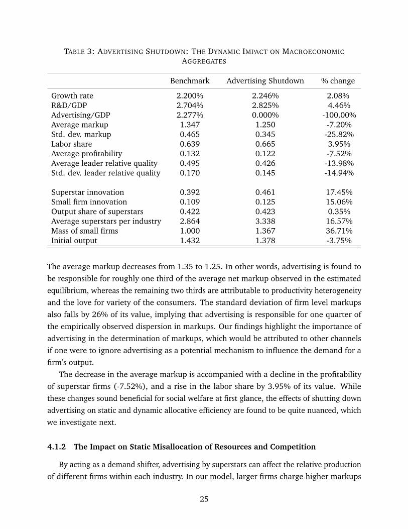
TABLE 3: ADVERTISING SHUTDOWN: THE DYNAMIC IMPACT ON MACROECONOMIC
AGGREGATES
Benchmark Advertising Shutdown % change
Growth rate 2.200% 2.246% 2.08%R&D/GDP 2.704% 2.825% 4.46%Advertising/GDP 2.277% 0.000% -100.00%Average markup 1.347 1.250 -7.20%Std. dev. markup 0.465 0.345 -25.82%Labor share 0.639 0.665 3.95%Average profitability 0.132 0.122 -7.52%Average leader relative quality 0.495 0.426 -13.98%Std. dev. leader relative quality 0.170 0.145 -14.94%
Superstar innovation 0.392 0.461 17.45%Small firm innovation 0.109 0.125 15.06%Output share of superstars 0.422 0.423 0.35%Average superstars per industry 2.864 3.338 16.57%Mass of small firms 1.000 1.367 36.71%Initial output 1.432 1.378 -3.75%
The average markup decreases from 1.35 to 1.25. In other words, advertising is found to
be responsible for roughly one third of the average net markup observed in the estimated
equilibrium, whereas the remaining two thirds are attributable to productivity heterogeneity
and the love for variety of the consumers. The standard deviation of firm level markups
also falls by 26% of its value, implying that advertising is responsible for one quarter of
the empirically observed dispersion in markups. Our findings highlight the importance of
advertising in the determination of markups, which would be attributed to other channels
if one were to ignore advertising as a potential mechanism to influence the demand for a
firm’s output.
The decrease in the average markup is accompanied with a decline in the profitability
of superstar firms (-7.52%), and a rise in the labor share by 3.95% of its value. While
these changes sound beneficial for social welfare at first glance, the effects of shutting down
advertising on static and dynamic allocative efficiency are found to be quite nuanced, which
we investigate next.
4.1.2 The Impact on Static Misallocation of Resources and Competition
By acting as a demand shifter, advertising by superstars can affect the relative production
of different firms within each industry. In our model, larger firms charge higher markups
25

which creates static misallocation: more productive firms do not demand enough labor and
produce too little relative to the efficient allocation. As a result, heterogeneous advertising,
by shifting market shares between incumbents, could directly affect the degree of static
allocative efficiency. We analyze this effect in this section.
The analysis in Appendix C.3 shows how advertising affects static allocative efficiency.
For a given industry state, it affects industry output by (i) influencing the relative output (yi)
of firms with different productivities, (ii) modifying the perceived quality (ωi) of different
varieties, and (iii) changing the relative wage.
In the previous section, we had established that shutting down advertising led to a
significant decrease in the average net markup and its dispersion by one third and one
quarter, respectively. Therefore, one might be tempted to expect an increase in allocative
efficiency. Surprisingly, we find the opposite result to be the case: shutting down advertising
reduces allocative efficiency, decreasing the level of output by 3.75% of its value.
This result owes to the two effects working in the opposite direction: First, advertising
is found to help reallocate production from less productive superstars to more efficient
superstars. This means that the economy with advertising uses resources more efficiently
even if we hold perceived quality fixed. Second, optimal advertising chosen by the superstars
in equilibrium is such that the perceived quality of large and more efficient superstars is
magnified compared to the smaller and less efficient superstars. This further amplifies
the gains from production by improving the perceived quality of the more abundant (or
cheaper to produce) varieties. Combined together, the reallocation of resources towards
more efficient firms, and the relative amplification of the perceived quality of the same,
work against the effects of higher markups; implying that advertising helps improve static
allocative efficiency on the net.
Focusing on how shutting down advertising affects allocative efficiency across different
industry states also reveals interesting patterns. Figure 4 depicts the difference in industry
output between our baseline model and our counterfactual economy as a function of industry
concentration measured by the HHI (taken from the baseline economy). It shows that the
decrease in industry output is larger for industries that are more concentrated. Advertising
allows larger firms to shift demand towards their products and away from those smaller
and less productive. This is further clarified in the left panel of Figure 5, which displays
the change in industry output as a function of productivity dispersion in the industry. As
seen in the figure, this reallocation of market shares, improving static allocative efficiency,
is stronger in industries where the dispersion in terms of productivity is larger. The right
panel of Figure 5 displays the reduction in the average industry markup once again as a
function of productivity dispersion. One can see that the decline of the average industry
26

FIGURE 4: CHANGE IN INDUSTRY OUTPUT BY MARKET CONCENTRATION
markup tends to be stronger in industries with higher productivity dispersion, but despite
its positive effects, the reallocation and perceived quality amplification channels dominate,
and we observe an overall decline in industry output across the board for all industry states.
FIGURE 5: CHANGE IN INDUSTRY OUTPUT AND MARKUP BY PRODUCTIVITY DISPERSION
4.1.3 Short-Run versus Long-Run Effects on Markups and Welfare
In this section, we investigate the short- and long-run effects of shutting down advertising
on markups and social welfare. First, we decompose our main results regarding markups
between the static and dynamic parts. The static part results from changes in markups due
to shutting down advertising for a given distribution over industry states. The dynamic effect
is due to the endogenous response of firms in terms of R&D investment when advertising
27

is shut down. This leads to a change in the distribution over industry states with different
markups. Second, we study the welfare implications of shutting down advertising, and
perform a similar decomposition between the short-run and long-run welfare changes.
Shutting down advertising changes industry output and static allocative efficiency as shown
in Section 4.1.2. In addition, it also affects R&D investment and hence both the stationary
distribution over industry states and the growth rate of the economy.
First, we can decompose the change in markups between our baseline calibration and
our counterfactual economy into a static and dynamic effect. Statically, advertising affects
the markups that superstar firm charge as well as the distribution of market shares within
industry. The change in aggregate markups between the two economies that results from
those changes for a fixed distribution over industry states is what we call the static effect of
advertising on markups. The dynamic effect arises from the impact of changes on advertising
on the R&D investment of superstar firms, which further leads to a change in the distribution
over industry states. This dynamic effect is the result of the equilibrium interaction between
advertising and R&D. Statically, we find that shutting down advertising reduces markups
by 5.58% from 1.35 to 1.27. The dynamic effect coming from the interaction between
advertising and R&D investment and its impact on the industry state distribution further
reduces markups by 1.71% to 1.25. At the same time, the dispersion of markups also goes
down when advertising is shut down (from 0.47 to 0.35). Around two thirds of this decrease
is due to the static effect of advertising, whereas the remainder owes to the long-run change
in the stationary distribution across industry states.
Second, regarding welfare, our model allows for an analytical decomposition of the
change in welfare (W) between our baseline calibration and our counterfactual economy
without advertising, as follows (see the details in Appendix B.3):
∆W =1ρ
[∆ ln ζ − ∆ ln wrel + ∆ ∑
Θf (Θ)µ(Θ) + ∆ ln
(CY
)]+
1ρ2 ∆g (41)
The first term in the square bracket corresponds to the change in the relative productivity
of the fringe across the two economies, the second term reflects the change in the relative
wage, and the third term relates to changes in the relative industry output of superstar
firms. These three terms collectively represent the change in welfare due to the change in
the initial output level, Y0. The fourth term captures changes in the consumption share of
GDP. The last term in the equation is the differential in the growth rates between the two
economies.
Table 4 shows how each of these components is affected by shutting down advertising.
28

TABLE 4: ADVERTISING SHUTDOWN: SHORT-RUN VS. LONG-RUN EFFECTS ON EFFICIENCY
Static Static+New Distribution Dynamic
∆W CEWC ∆W CEWC ∆W CEWC
Competitive fringe productivity 0.000 0.00% 0.000 0.00% 0.000 0.00%Relative wage -0.812 -3.19% -0.968 -3.80% -0.968 -3.80%Output of superstar firms -0.500 -1.98% 0.013 0.05% 0.013 0.05%Consumption/GDP 0.593 2.40% 0.593 2.40% 0.534 2.16%Output growth 0.000 0.00% 0.000 0.00% 0.286 1.15%
Total -0.718 -2.83% -0.362 -1.44% -0.134 -0.54%
Overall, we obtain a welfare loss of 0.54% in consumption-equivalent terms.14 The first
two columns in the table report the static effect of advertising on welfare, i.e. fixing the
distribution over industry states and the level of R&D. Statically, shutting down advertising
results in a large welfare loss of 2.83%, which comes from the resulting decrease in the
relative wage and in output of superstar firms. As discussed in Section 4.1.2, shutting down
advertising reduces static allocative efficiency, which results in a welfare loss. The third and
fourth columns in Table 4 display what happens to welfare if we further let the distribution
adjust (but still keep R&D and growth fixed). In that case, the welfare loss from shutting
down advertising is smaller. This is due to the fact that the industry state distribution
shifts towards industries in which superstars produce more. As a result, total output of
superstars increases which results in welfare gains. On the other hand, the relative wage
further decreases. Finally, the last two columns of Table 4 show the full results including the
dynamic effects due to changes in R&D investment. Shutting down advertising raises the
consumption-to-output ratio as a result of changes in total R&D and advertising expenses.
In addition, the growth rate of the economy increases. Overall, these dynamic effects further
offset some of the static welfare losses. All in all, static losses are larger than dynamic gains,
resulting in a total welfare loss of 0.54% in consumption equivalent terms when advertising
is shut down. Therefore, we conclude that advertising, despite its various negative effects,
helps rather than hurts efficiency, albeit by a small margin.
14Consumption-equivalent welfare is defined as the compensation in lifetime consumption that the represen-tative household from one economy requires to remain indifferent between consuming in this economy versusconsuming in the counterfactual economy. This welfare measure is provided in equation (B.8) of AppendixB.3.
29

4.2 Should We Tax or Subsidize Advertising?
Our results so far raise some questions in terms of policy implications, especially regard-
ing advertising. Our results from Section 4.1.3 show that totally shutting down advertising
is not socially desirable as it reduces welfare. In this section, we study whether a subsidy or
a tax on advertising could be welfare-improving. In particular, we focus on linear taxes and
subsidies. The revenues from taxes are rebated back to the consumers, and subsidies are
financed through lump-sum taxes.
Table 5 reports the results of our policy experiment for different values of taxes and
subsidies.15 In line with the results of our shutdown experiment, higher taxes (subsidies)
on advertising are associated with a reduction (increase) in advertising expenditures and an
increase (decrease) in R&D intensity. That is, the substitution effect between advertising
and R&D dominates. Taxing advertising also results in a decrease in average markup and
its dispersion and in an increase in the labor share. At the same time, raising taxes also
decreases the level of initial output as static allocative efficiency worsens. The decrease in
advertising expenditures along with the lump-sum rebate of the tax results in an increase
in initial consumption at low levels of the tax rate. As the tax rate keeps increasing, the
decrease in initial output due to losses in static allocative efficiency dominates, and initial
consumption starts decreasing.
FIGURE 6: THE DYNAMIC WELFARE IMPACT OF ADVERTISING TAXES
Overall, we have several forces associated with taxation or subsidization of advertising
15Note that reported tax and subsidy rates correspond to the share of total advertising-related expenses thatare collected as tax or paid as subsidies by the government.
30

that go in opposite directions regarding welfare. We find that there exists an optimal level
of tax on advertising that maximizes welfare equal to 64.6% (see Figure 6). This tax is
associated to a 0.9% increase in growth, a 1.2% increase in R&D intensity, a 10% reduction
in the average markup and 8.6% reduction in markup dispersion, a 1.4% increase in the
labor share, a 1.6% reduction in initial output, a 8.6% increase in the mass of small firms,
and an overall increase in welfare of 0.6%. Subsidies, on the other hand, only serve to
reduce welfare.
Section 4.1.3 established that shutting down advertising improved welfare. How does
one reconcile this finding with the fact that the optimal linear tax on advertising is found
to be quite high at 64.6%? The answer lies in understanding how taxation differs from
a complete shutdown. Higher taxes on advertising expenses discourage the firms from
investing resources into advertising, resulting in both direct gains in the consumption-
to-output ratio, and indirect gains from improved incentives for innovation and growth.
However, the taxes do not cause as large a drop in static allocative efficiency as a complete
shutdown would: while the overall spending on advertising declines, more productive
superstars still continue to spend more on advertising than less productive ones. Therefore,
the positive effects of advertising due to the more efficient reallocation of resources are still
present even under high tax rates. In other words, the taxes reduce the excessive spending
on advertising due to the “rat race” between the superstars, while still largely preserving
the relative market shares in equilibrium. This makes advertising a perfect candidate for
taxation.
In most advanced economies including the United States, advertising expenses are not
taxed. Our quantitative analysis demonstrates that advertising is a useful activity insofar
that it improves static allocative efficiency through a reduction in the misallocation of
resources. However, the same useful effects can largely be attained under relatively high
linear taxes, while eliminating most of the excessive spending that arises due to its “rat
race” nature. Given that most taxes that governments levy to finance government spending
unambiguously reduce efficiency rather than boost it, taxing advertising seems like a great
alternative, which can be used to raise a significant amount of revenue while simultaneously
improving dynamic efficiency. While the optimal level calculated at 64.6% may seem
rather high, this is well within the range European countries levy on petroleum products,
which create a large dead-weight loss as well as increase transportation costs. In such a
world of second-bests, taxation of advertising expenditures seems to be an idea well worth
investigating, all the more so given that advertising expenditures are found to be very
inelastic to the taxes levied.
31

TABLE 5: THE DYNAMIC IMPACT OF ADVERTISING TAXES AND SUBSIDIES ON MACROECONOMIC
AGGREGATES
Benchmark 25% Tax % change 50% Tax % change 75% Tax % changeGrowth rate 2.200% 2.206% 0.26% 2.214% 0.62% 2.226% 1.19%R&D/GDP 2.704% 2.709% 0.18% 2.722% 0.64% 2.751% 1.71%Advertising/GDP (after-tax) 2.277% 2.091% -8.16% 1.831% -19.59% 1.405% -38.31%Average markup 1.347 1.337 -0.73% 1.324 -1.71% 1.304 -3.21%Std. dev. markup 0.465 0.453 -2.52% 0.438 -5.92% 0.413 -11.18%Labor share 0.639 0.642 0.38% 0.645 0.89% 0.650 1.70%Average profitability 0.132 0.131 -0.95% 0.129 -2.21% 0.127 -4.07%Average leader relative quality 0.495 0.490 -1.07% 0.482 -2.70% 0.468 -5.58%Std. dev. leader relative quality 0.170 0.168 -1.07% 0.166 -2.55% 0.161 -5.13%
Superstar innovation 0.392 0.397 1.17% 0.404 3.07% 0.418 6.62%Small firm innovation 0.109 0.110 1.44% 0.113 3.75% 0.117 7.81%Output share of superstars 0.422 0.421 -0.22% 0.420 -0.40% 0.420 -0.43%Average superstars per industry 2.864 2.896 1.11% 2.947 2.90% 3.043 6.26%Mass of small firms 1.000 1.021 2.10% 1.055 5.46% 1.120 12.01%Initial output 1.432 1.425 -0.53% 1.415 -1.16% 1.404 -1.99%C.E. welfare change 0.346% 0.567% 0.578%
Optimal Tax % change 15% Subsidy % change 25% Subsidy % change(64.6%)
Growth rate 2.220% 0.92% 2.197% -0.15% 2.194% -0.26%R&D/GDP 2.736% 1.16% 2.703% -0.04% 2.703% -0.06%Advertising/GDP (after-tax) 1.614% -29.09% 2.381% 4.59% 2.461% 8.07%Average markup 1.313 -2.49% 1.353 0.43% 1.357 0.76%Std. dev. markup 0.425 -8.64% 0.472 1.47% 0.477 2.62%Labor share 0.648 1.31% 0.638 -0.22% 0.637 -0.39%Average profitability 0.128 -3.19% 0.133 0.56% 0.134 0.99%Average leader rel. quality 0.475 -4.15% 0.498 0.57% 0.500 1.00%Std. dev. leader rel. quality 0.164 -3.83% 0.171 0.64% 0.172 1.16%
Superstar innovation 0.411 4.83% 0.390 -0.59% 0.388 -1.03%Small firm innovation 0.115 5.83% 0.108 -0.72% 0.107 -1.23%Output share of superstars 0.420 -0.45% 0.422 0.16% 0.423 0.29%Average superstars per industry 2.995 4.57% 2.848 -0.56% 2.836 -0.98%Mass of small firms 1.086 8.65% 0.989 -1.10% 0.981 -1.94%Initial output 1.409 -1.61% 1.437 0.33% 1.440 0.58%C.E. welfare change 0.612% -0.304% -0.618%
32

5 Conclusion
Firms routinely make intensive use of their innovation and advertising expenditures
in order to alter the perceived quality of their products, allowing them to shift consumer
demand toward themselves and gain market share in their industry. At the aggregate level,
these two forms of intangible investments make up for a large share of GDP in the United
States. Yet, the interaction between them and their implications for economic growth and
social welfare remain understudied in the economics literature. In this paper, we have
proposed a unified approach to study the interaction between advertising and innovation in
a heterogeneous-firm model in which market structure (i.e. the number of large firms and
their share of the industry’s total output), markups and growth are all endogenous. In the
model, large firms make production, innovation, and advertising choices strategically in an
oligopolistic environment, and small firms spend resources on R&D to gain access to the
pool of large firms. In equilibrium, large firms of different productivities use advertising
strategically to gain market share and charge higher markups, which has implications for
allocative efficiency. Dynamically, advertising and innovation choices interact and, at the
aggregate level, affect the pace of economic growth.
We estimate the model to match features of the data at different levels of aggregation,
and particularly to fit the existing non-linear relationship between innovation, advertising,
and competition in the data. We find that advertising has important quantitative implications
for macroeconomic aggregates. Specifically, shutting down advertising leads to a decrease
in allocative efficiency, because advertising reallocates market shares toward larger and
more productive firms. However, as in the estimated model, advertising and innovation are
substitutes, shutting down advertising frees up resources for firms to use in their innovation
expenditures, which boosts economic growth. This substitution effect is in line with the
empirical findings in Cavenaile and Roldan-Blanco (2021). All in all, while the average
net markup decreases by one third of its value relative to the baseline estimation when
advertising is shut down, the rate of economic growth increases by about 2%. However,
we find that advertising helps static allocative efficiency through reallocating resources
towards more efficient firms, and its shutdown therefore reduces static efficiency. Overall,
static losses are larger than dynamic gains, resulting in a total welfare loss of 0.54% in
consumption-equivalent terms, implying that advertising is a useful economic activity on
the net.
In the last part of the paper, we ask whether advertising should be subsidized or taxed
on the basis of our estimated model. We find that advertising should be taxed, and that
the optimal advertising tax (that is, the tax that maximizes long-run social welfare) would
33

lead to a 0.9% increase in growth, a 10% reduction in the average markup, and a 1.4%
increase in the labor share, for an overall increase in welfare of 0.6%. In other words,
despite its positive effects on static allocative efficiency, a linear tax levied on advertising
can still improve welfare since it can reduce the excessive spending that is due to the “rat
race” nature of advertising. We believe that these results are relevant for industrial policy
as well as public finance, and expect future research to delve further into this and other
topics relating the interaction between firm intangibles with competition, growth, and social
welfare.
34

References
AGHION, P., A. BERGEAUD, T. BOPPART, P. J. KLENOW, AND H. LI (2019): “A Theory of
Falling Growth and Rising Rents,” NBER Working Paper No. 26448.
AKCIGIT, U., AND S. T. ATES (2019a): “Ten Facts on Declining Business Dynamism and
Lessons from Endogenous Growth Theory,” American Economic Journal: Macroeconomics,forthcoming.
(2019b): “What Happened to US Business Dynamism?,” NBER Working Paper No.25756.
ATKESON, A., AND A. BURSTEIN (2008): “Pricing-to-Market, Trade Costs, and International
Relative Prices,” American Economic Review, 98(5), 1998 – 2031.
BAGWELL, K. (2007): “The Economic Analysis of Advertising,” Handbook of IndustrialOrganization, 3, 1701 – 1844.
BAQAEE, D. R., AND E. FARHI (2020): “Productivity and misallocation in general equilibrium,”
The Quarterly Journal of Economics, 135(1), 105–163.
BARKAI, S. (2020): “Declining Labor and Capital Shares,” The Journal of Finance, p.
jofi.12909.
BECKER, G. S., AND K. M. MURPHY (1993): “A Simple Theory of Advertising as a Good or
Bad,” The Quarterly Journal of Economics, 108(4), 941 – 964.
BELO, F., X. LIN, AND A. M. VITORINO (2014): “Brand capital and firm value,” Review ofEconomic Dynamics, 17(1), 150 – 169.
BENHABIB, J., AND A. BISIN (2002): “Advertising, Mass Consumption and Capitalism,”
Working Paper, New York University.
BURSTEIN, A., V. M. CARVALHO, AND B. GRASSI (2020): “Bottom-up Markup Fluctuations,”
Working paper.BUTTERS, G. R. (1977): “Equilibrium Distributions of Sales and Advertising Prices,” The
Review of Economic Studies, 44(3), 465 – 491.
CAVENAILE, L., M. A. CELIK, AND X. TIAN (2020): “Are Markups Too High? Competition,
Strategic Innovation, and Industry Dynamics,” Working paper.CAVENAILE, L., AND P. ROLDAN-BLANCO (2021): “Advertising, Innovation and Economic
Growth,” American Economic Journal: Macroeconomics, forthcoming.
CROUZET, N., AND J. C. EBERLY (2019): “Understanding Weak Capital Investment: The Role
of Market Concentration and Intangibles,” NBER Working Paper 25869.
DE LOECKER, J., J. EECKHOUT, AND G. UNGER (2020): “The Rise of Market Power and the
Macroeconomic Implications,” The Quarterly Journal of Economics, 135(2), 561 – 644.
DERIDDER, M. (2020): “Market Power and Innovation in the Intangible Economy,” Working
35

paper.DINLERSOZ, E. M., AND M. YORUKOGLU (2012): “Information and Industry Dynamics,”
American Economic Review, 102(2), 884 – 913.
DORFMAN, R., AND P. O. STEINER (1954): “Optimal Advertising and Optimal Quality,”
American Economic Review, 44(5), 826 – 836.
DROZD, L. A., AND J. B. NOSAL (2012): “Understanding International Prices: Customers as
Capital,” American Economic Review, 102(1), 364 – 395.
EDMOND, C., V. MIDRIGAN, AND D. Y. XU (2018): “How Costly Are Markups?,” NBERWorking Paper No. 24800.
ERICKSON, T., AND T. WHITED (2002): “Two-step GMM Estimation of the Errors-invariables
Model using High-order Moments,” Econometric Theory, 18, 776–799.
FITZGERALD, D., S. HALLER, AND Y. YEDID-LEVI (2017): “How Exporters Grow,” WorkingPaper, Federal Reserve Bank of Minneapolis.
GOURIO, F., AND L. RUDANKO (2014): “Customer Capital,” Review of Economic Studies, 81(3),
1102 – 1136.
GREENWOOD, J., Y. MA, AND M. YORUKOGLU (2020): “‘You Will’: A Macroeconomic Analysis
of Digital Advertising,” Working paper.HALL, B. H., A. B. JAFFE, AND M. TRAJTENBERG (2001): “The NBER Patent Citation Data
File: Lessons, Insights and Methodological Tools,” NBER Working Paper No. 8498.
KARABARBOUNIS, L., AND B. NEIMAN (2013): “The Global Decline of the Labor Share,” TheQuarterly Journal of Economics, 129(1), 61–103.
LIU, E., A. MIAN, AND A. SUFI (2019): “Low Interest Rates, Market Power, and Productivity
Growth,” NBER Working Paper No. 25505.
MOLINARI, B., AND F. TURINO (2017): “Advertising and Aggregate Consumption: A Bayesian
DSGE Assessment,” The Economic Journal, 128(613), 2106 – 2130.
MORLACCO, M., AND D. ZEKE (2020): “Monetary Policy, Customer Capital, and Market
Power,” Working paper.PERLA, J. (2019): “Product Awareness, Industry Life Cycles, and Aggregate Profits,” Working
Paper, University of British Columbia.
PETERS, M. (2020): “Heterogeneous Mark-Ups, Growth and Endogenous Misallocation,”
Econometrica, 88(5), 2037–2073.
PETERS, M., AND C. WALSH (2019): “Declining Dynamism, Increasing Markups and Missing
Growth: The Role of The Labor Force,” Working paper.RACHEL, L. (2021): “Leisure-Enhancing Technological Change,” Working paper.ROLDAN-BLANCO, P., AND S. GILBUKH (2021): “Firm Dynamics and Pricing under Customer
Capital Accumulation,” Journal of Monetary Economics, forthcoming.
36

WEISS, J. (2019): “Intangible Investment and Market Concentration,” Working paper.
37

Online Appendix for “Style Over Substance?
Advertising, Innovation, and Endogenous Market
Structure”
by Laurent Cavenaile, Murat Alp Celik, Pau Roldan-Blanco, and Xu Tian
A Estimation Details
The model has 12 parameters to be determined: the innovation step size λ, the cost
scale parameters for superstars and small firms (χ, ν), the corresponding cost curvature
parameters (φ, ε), the relative productivity between the leader and the fringe ζ, the exit
rate τ, the entry cost scale ψ, the cost scale and curvature parameters in the advertising
cost function (χa, φa), the elasticity among superstars’ outputs within an industry η, and the
elasticity between the superstars’ output and the fringe’s output γ. These 12 parameters
are jointly estimated via a Simulated Method of Moments (SMM) estimation procedure to
match 14 moments in the data.
The simulated moments estimator is defined as the solution to the minimization of
weighted average distance between data and model moments. We calculate the optimal
weight matrix using influence function method following Erickson and Whited (2002). We
use a simulated annealing algorithm to minimize the objective function. This starts with a
predefined first and second guess. For the third guess onward, it takes the best prior guess
and randomizes from this to generate a new set of parameter guesses. That is, it takes
the best-fit parameters and randomly “jumps off” from this point for its next guess. Over
time the algorithm “cools”, so that the variance of the parameter jumps falls, allowing the
estimator to fine-tune its parameter estimates around the global best fit. We restart the
program with different initial conditions to ensure the estimator converges to the global
minimum. The simulated annealing algorithm is extremely slow, which restricts the size of
the parameter space that can be estimated. Nevertheless, we use this because it is robust
to the presence of local minima and discontinuities in the objective function across the
parameter space.
In the estimation, we set the maximum number of superstars in an industry to N = 4and the maximum productivity step size to n = 5, which delivers 84 unique industry states
Θ. The results do not significantly change if we increase n or N. The estimated value of λ
adjusts to absorb the choice of a different n. The relative productivity of the competitive
fringe ζ adjusts to absorb the changes in N. In the estimated model, n is chosen large
i
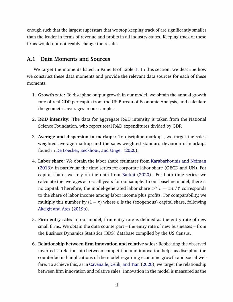
enough such that the largest superstars that we stop keeping track of are significantly smaller
than the leader in terms of revenue and profits in all industry-states. Keeping track of these
firms would not noticeably change the results.
A.1 Data Moments and Sources
We target the moments listed in Panel B of Table 1. In this section, we describe how
we construct these data moments and provide the relevant data sources for each of these
moments.
1. Growth rate: To discipline output growth in our model, we obtain the annual growth
rate of real GDP per capita from the US Bureau of Economic Analysis, and calculate
the geometric averages in our sample.
2. R&D intensity: The data for aggregate R&D intensity is taken from the National
Science Foundation, who report total R&D expenditures divided by GDP.
3. Average and dispersion in markups: To discipline markups, we target the sales-
weighted average markup and the sales-weighted standard deviation of markups
found in De Loecker, Eeckhout, and Unger (2020).
4. Labor share: We obtain the labor share estimates from Karabarbounis and Neiman
(2013); in particular the time series for corporate labor share (OECD and UN). For
capital share, we rely on the data from Barkai (2020). For both time series, we
calculate the averages across all years for our sample. In our baseline model, there is
no capital. Therefore, the model-generated labor share wrel L = wL/Y corresponds
to the share of labor income among labor income plus profits. For comparability, we
multiply this number by (1− κ) where κ is the (exogenous) capital share, following
Akcigit and Ates (2019b).
5. Firm entry rate: In our model, firm entry rate is defined as the entry rate of new
small firms. We obtain the data counterpart – the entry rate of new businesses – from
the Business Dynamics Statistics (BDS) database compiled by the US Census.
6. Relationship between firm innovation and relative sales: Replicating the observed
inverted-U relationship between competition and innovation helps us discipline the
counterfactual implications of the model regarding economic growth and social wel-
fare. To achieve this, as in Cavenaile, Celik, and Tian (2020), we target the relationship
between firm innovation and relative sales. Innovation in the model is measured as the
ii

Poisson arrival event of quality improvement, whereas it is measured as average patent
citations for each firm in the data.16 We normalize both by subtracting their means
and dividing by the standard deviation. In the data, we regress average citations on
relative sales of the firm in its SIC4 industry and its square. The control variables
include profitability, leverage, market-to-book ratio, log R&D stock, firm age, the
coefficient of variation of the firm’s stock price, the number of firms in the industry,
and a full set of year and SIC4 industry fixed effects. We target the linear and quadratic
terms of a regression of (standardized) average citations on relative sales.
7. Average profitability: In the model, average profitability is calculated as static profit
flow minus R&D expenses divided by sales. In the data, it is defined as operating
income before depreciation divided by sales (OIBDP/SALE in Compustat.)
8. Average and dispersion in leader relative quality: We target the average relative
quality of the leader in an industry, and its standard deviation across all industries. In
the model, quality is known. In the data, we proxy quality by calculating the stock of
past patent citations. The relative quality of the leader is defined as the quality of the
leader divided by the sum of the qualities of the top four firms in an industry (SIC4 in
the data.)
9. Advertising share of GDP: The aggregate advertising expenses over GDP ratio is
calculated based on the Coen Structured Advertising Expenditure Dataset, extracted
from the McCann Erikson advertising agency.17
10. Relationship between firm advertising and relative sales: Replicating the observed
inverted-U relationship between competition and advertising also helps use discipline
the counterfactual implications of the model regarding economic growth and social
welfare. Therefore, we also require the model-generated relationship between firm
advertising expenses and relative sales to be the same as in the data. We regress the
logarithm of firm advertising expenses (log(1+xad)) on relative sales of the firm in
its SIC4 industry and its square. The control variables include profitability, leverage,
market-to-book ratio, log R&D stock, firm age, the coefficient of variation of the firm’s
16To measure patent citation, we use the patent grant data obtained from NBER Patent Database Projectwhich covers the years 1976-2006. We reply on Compustat North American Fundamentals for financialstatement information of US-listed firms for the same years. Following a dynamic assignment procedure, welink the two data sets. We measure innovation as the number of citations a patent received as of 2006. Weuse the truncation correction weights devised by Hall, Jaffe, and Trajtenberg (2001) to correct for systematiccitation differences across different technology classes and for the fact that earlier patents have more yearsduring which they can receive citations (truncation bias).
17The data is available at http://www.purplemotes.net/2008/09/14/us-advertising-expenditure-data/.
iii
stock price, the number of firms in the industry, and a full set of year and SIC4 industry
fixed effects. We normalize the advertising expenses in both the data and model
by subtracting their means and dividing by the standard deviation, and target the
coefficients for the linear and quadratic terms of the regression after normalization.
A.2 Identification
The model is highly nonlinear, and all parameters affect all the moments. Nevertheless,
some parameters are more important for certain statistics. The success of SMM estimation
depends on model identification, which requires that we choose moments that are sensitive
to variations in the structural parameters. We now rationalize the moments that we choose
to match.
Table A.1 reports the Jacobian matrix associated with the estimation of the baseline
model. Each entry of the matrix reports the percentage change in each moment given one
percent increase in each parameter. This table gives us some indication on which data
moments are most informative in helping us identifying each parameter:
(i) The productivity step size parameter λ is mainly identified by the output growth rate.
A higher λ implies a higher increase in firm productivity upon successful innovation,
which leads to higher output growth rate.
(ii) Average profitability and the standard deviation of markups are most helpful in
identifying the elasticity of substitution between superstar firms η and the elasticity of
substitution between superstar and small firms γ. Larger γ implies higher substitution
between superstar and small firms, which leads to lower market power, profitability,
and heterogeneity in markups across firms. Larger η implies higher substitution
among superstars, which creates higher incentives for leading superstar firms to
invest in advertising to shift demand and profits toward their products. This, in turn,
leads to slightly higher average markups, profitability, and heterogeneity in markups
across firms. The average and standard deviation of leader relative quality increase
accordingly.
(iii) An increase in either superstar innovation cost scale parameter χ or small firm innova-
tion cost scale parameter ν reduces the aggregate R&D intensity and output growth
rate. Since superstar innovation has a direct effect on the growth rate of the economy,
the effect of χ on the output growth rate relative to its effect on R&D intensity is larger,
whereas ν has a larger impact on R&D intensity. In addition, χ and ν have opposite
implications for the level and dispersion of leader quality. Overall, larger χ tends to
iv

TABLE A.1: IDENTIFICATION: JACOBIAN MATRIX
λ η χ ν ζ φ
Growth rate 0.866 -0.052 -0.248 -0.031 -0.309 2.029R&D/GDP 0.021 -0.121 -0.191 -0.054 -1.119 1.021Advertising/GDP -0.784 -0.304 0.041 -0.091 -1.100 0.197Average markup 0.115 0.002 -0.001 0.002 -0.210 -0.009Std. dev. markup 0.675 0.100 -0.014 0.027 -0.237 -0.052Labor share -0.023 0.010 -0.001 0.002 0.174 0.001Entry rate 0.000 0.000 0.000 0.000 0.000 0.000Avg profitability 0.266 0.012 0.036 0.014 -0.672 -0.230Avg leader rel. quality 0.497 0.139 -0.033 0.072 0.260 -0.089Std. dev. leader rel. quality 0.371 0.181 -0.058 0.106 0.367 0.233β(innovation, rel. sales) 0.288 0.007 -0.157 0.036 0.109 -0.028Top point (innovation, rel. sales) 0.295 0.079 0.000 0.003 0.130 -0.207β(advertising, rel. sales) -0.553 -0.161 0.003 -0.003 -0.195 -0.037Top point (advertising, rel. sales) 0.336 0.152 0.011 -0.021 0.086 -0.075
ε χa φa γ ψ τ
Growth rate 0.198 0.009 0.037 -0.229 -0.055 -0.096R&D/GDP 0.344 0.004 0.066 -0.620 -0.095 -0.167Advertising/GDP 0.636 -0.283 -0.558 -0.331 -0.158 -0.279Average markup -0.005 -0.026 -0.058 -0.101 0.003 0.005Std. dev. markup -0.165 -0.089 -0.262 -0.331 0.048 0.084Labor share -0.016 0.013 0.022 0.063 0.003 0.006Entry rate 0.000 0.000 0.000 0.000 0.000 1.000Avg profitability -0.086 -0.034 -0.050 -0.216 0.025 0.043Avg leader rel. quality -0.485 -0.036 -0.124 0.264 0.125 0.220Std. dev. leader rel. quality -0.579 -0.039 -0.163 0.324 0.184 0.324β(innovation, rel. sales) -0.181 0.036 -0.077 0.039 0.062 0.109Top point (innovation, rel. sales) -0.022 -0.021 -0.100 0.181 0.006 0.010β(advertising, rel. sales) -0.007 0.075 0.127 -0.568 -0.005 -0.010Top point (advertising, rel. sales) 0.119 -0.055 -0.149 0.318 -0.037 -0.064
Notes: The table shows the Jacobian matrix associated with the estimation of the baseline model. Each entryof the matrix reports the percentage change in each moment given one percent increase in each parameter.
v

reduce the innovation of superstar firms, narrowing the quality gaps between the
industry leader and other superstar firms. While higher ν increases the R&D cost of
small firms, which reduces their innovation, leading to a reallocation of market share
to superstar firms and a higher heterogeneity in qualities among superstar firms.
(iv) The relative productivity of small firms ζ is identified very precisely by matching the
average markup and the labor share. Lower ζ implies reduced competition from
small firms and a within-industry market share reallocation to superstar firms, which
generates a higher average markup and lower labor share.
(v) As innovation policies in our estimated model are below unity, an increase in the
R&D cost convexity parameters φ and ε reduces the innovation cost, which increases
R&D intensity and the growth rate. These two parameters, however, have different
implications for inverted-U relationship between innovation and market shares. While
ε strongly influences the linear coefficient of the innovation-market share regression,
changes in φ mainly affect the location of the top point of the inverted-U relationship.
The two parameters’ impacts on the standard deviation of leader relative quality are
also opposite.
(vi) Intuitively, the three advertising-related data moments are most informative in helping
us identify the two parameters governing the cost scale and curvature parameters in
the advertising cost function, (χa, φa). While all the advertising related moments are
affected by these two parameters in the same direction, overall they are more sensitive
to the changes in φa. The two parameters’ impacts on linear term of innovation-market
share regression are also opposite.
(vii) The exogenous exit rate parameter τ is directly identified by targeting the entry rate of
new businesses, since firm entry rate equals firm exit rate in a stationary equilibrium.
(viii) Given all other parameter values, the value of ψ is set to normalize the measure of
small firms mt to one. Its exact value hinges on the average value of small firms, which
itself is determined by the values of all other parameters. In particular, setting m = 1,
we can rewrite equation (36) to get ψ = ∑Θ ve(Θ)µ(Θ)2τ .
vi

B Additional Derivations and Proofs
B.1 Derivation of the growth rate
This section derives the growth rate of the economy. Using the production function at
the aggregate and industry levels, we can write:
ln(Yt) =∫ 1
0
γ
γ− 1ln
yγ−1
γ
cjt +
Njt
∑i=1
ωijtyη−1
η
ijt
η(γ−1)γ(η−1)
dj
=∫ 1
0
γ
γ− 1ln
yγ−1
γ
cjt
1 +
Njt
∑i=1
ωijt
(yijt
ycjt
) η−1η
η(γ−1)γ(η−1)
dj
=∫ 1
0
ln(ycjt)+
γ
γ− 1ln
1 +
Njt
∑i=1
ωijt
(yijt
ycjt
) η−1η
η(γ−1)γ(η−1)
dj
=∫ 1
0
ln
(qcjt
wrelt
σcjt
)+
γ
γ− 1ln
1 +
Njt
∑i=1
ωijt
(yijt
ycjt
) η−1η
η(γ−1)γ(η−1)
dj
=∫ 1
0
ln
(qcjt
wrelt
)+
1γ− 1
ln
1 +
Njt
∑i=1
ωijt
(yijt
ycjt
) η−1η
η(γ−1)γ(η−1)
dj
=∫ 1
0ln
(qcjt
wrelt
)dj + ∑
Θft(Θ)µt(Θ) (B.1)
where we have used that ycjt = qcjtlcjt = qcjtσcjt
wrelt
and σcjt =
1 +
Njt
∑i=1
ωijt
(yijt
ycjt
) η−1η
η(γ−1)γ(η−1)
−1
to arrive at the final expression. For a time step of size ∆ ≈ 0, we have:
ln(Yt+∆t)− ln(Yt) = − ln(wrelt+∆t) + ln(wrel
t ) + ln(1 + λ)∑Θ
plit(Θ)∆tµt(Θ)
+∑Θ
∑Θ′
[ft(Θ′)− ft(Θ)
]pt(Θ, Θ′)µt(Θ)∆t + o(∆t) (B.2)
vii

Dividing through by ∆ and taking the limit as ∆→ 0 we obtain:
gt = −gwrel ,t + ln(1 + λ)∑Θ
plit(Θ)µt(Θ) + ∑Θ
∑Θ′
[ft(Θ′)− ft(Θ)
]pt(Θ, Θ′)µt(Θ) (B.3)
B.2 Proof of Proposition 1
Let Θ denote the set of all industry-states Θ. Let h : Θ→ R be a function. Then:
E
[∑Θ′
p(Θ, Θ′)(h(Θ′)− h(Θ))
]= ∑
Θ∑Θ′
p(Θ, Θ′)(h(Θ′)− h(Θ))µ(Θ)
= ∑Θ
∑Θ′
p(Θ, Θ′)h(Θ′)µ(Θ)−∑Θ
∑Θ′
p(Θ, Θ′)h(Θ)µ(Θ)
= ∑Θ′
h(Θ′)∑Θ
p(Θ, Θ′)µ(Θ)−∑Θ
h(Θ)∑Θ′
p(Θ, Θ′)µ(Θ)
= ∑Θ′
h(Θ′)µ(Θ′)−∑Θ
h(Θ)µ(Θ)
= E[h(Θ′)
]−E [h(Θ)]
= 0
B.3 Calculating Social Welfare Metrics
In this Appendix, we detail how to compute welfare for the representative household,
as well as our measure of consumption-equivalent welfare changes, in a BGP. Along a
BGP, household consumption grows at the same rate as aggregate output. Therefore, the
stream of present-discounted value of utility from consumption can be summarized by two
variables: an initial level of consumption, C0, and the growth rate of the economy, g.
To compute initial output, use equation (B.1) to write:
Y0 = exp
(∫ 1
0ln(qcj0)dj− ln(wrel) + ∑
Θf (Θ)µ(Θ)
)(B.4)
In a BGP, all the terms are time-invariant, and we fix the average log productivity level
of fringe firms at time zero,∫ 1
0 ln(qcj0)dj, to zero in all counterfactual economies without
viii
loss of generality.18 The initial level of consumption is then given by:
C0 = Y0 ·C0
Y0= Y0
1 +∫ 1
0
Nj0
∑i=1
χzφij0 dj +
∫ 1
0
Nj0
∑i=1
χaωφaij0 dj +
∫ 1
0m0νXε
kj0 dj + ψe20
(B.5)
where we have used the aggregate resource constraint (equation (37)) at t = 0 on the
right-hand side. The welfare of the representative household can be found by imposing BGP
to equation (1):
W =∫ +∞
0e−ρt ln(Ct) dt =
1ρ
(ln(C0) +
gρ
)(B.6)
Using formulas (B.4) and (B.5), equation (41) readily follows. Finally, to compute
consumption-equivalent welfare changes between two economies A and B in their BGPs, we
compute the percentage change ς in lifetime consumption that the representative household
of economy A would require to remain indifferent between living in economy A and living
in economy B, that is:
WB =1ρ
(ln(
CA0 (1 + ς)
)+
gA
ρ
)(B.7)
Solving for ς, we get:
ς =CB
0
CA0
exp(
gB − gA
ρ
)− 1 (B.8)
C Social Planner’s Problem
There exist both static and dynamic distortions in the economy. Statically, there are
efficiency losses from the misallocation of labor both within and across industries due
to the presence of market power. Moreover, there are efficiency losses coming from the
choice of advertising, as firms do not internalize the effects that their advertising choices
have on markup dispersion and the profits of other firms. Dynamically, resources for R&D
are misallocated because firms fail to internalize the positive aggregate effects of their
innovations on economic growth, as well as the negative contribution of their innovation
resulting from business-stealing externalities.
18Because fringe firms keep a constant distance ζ with respect to their industry’s leader by assumption, thisassumption means that we keep the initial frontier technology level fixed across all counterfactual economies.
ix

C.1 The Complete Social Planner’s Problem
The goal of the social planner is to maximize the lifetime utility of the representative
household subject to the technological constraints of the economy. Given the initial condi-
tions, µ0(Θ), m0 and aggregate productivity Q0, the full problem can be stated as follows:
max[[{lijt,ωijt,zijt}
Njti=1,[lckjt,Xkjt]
mtk=0:j∈[0,1]
],et :t∈R+
] ∫ +∞
0e−ρt ln(Ct)dt (C.1)
subject to
Ct + RtYt + AtYt ≤ Yt (C.2a)
Rt =∫ 1
0
Njt
∑i=1
χzφijt +
∫νXε
kjtdk
dj + ψe2t (C.2b)
At =∫ 1
0
Njt
∑i=1
χaωφaijt dj (C.2c)
ln(Yt) =∫ 1
0ln(yjt)dj (C.2d)
yjt =
(y
γ−1γ
sjt + yγ−1
γ
cjt
) γγ−1
(C.2e)
ysjt =
Njt
∑i=1
ωijtyη−1
η
ijt
η
η−1
(C.2f)
ωijt =1 + ωijt
1Njt
∑Njti=1(1 + ωijt)
(C.2g)
ycjt =∫
yckjtdk (C.2h)
yijt = qijtlijt (C.2i)
yckjt = qcjtlckjt (C.2j)∫ 1
0
Njt
∑i=1
lijt +∫
lckjtdk
dj ≤ L = 1 (C.2k)
qleaderjt = max{q1jt, ..., qNjt jt} (C.2l)
qcjt = ζqleaderjt (C.2m)
{q1jt, ..., qNjt jt} ={
qleaderjt ,
qleaderjt
(1 + λ)~njt(1), ...,
qleaderjt
(1 + λ)~njt(Njt−1)
}(C.2n)
x

Θjt = (Njt,~njt) (C.2o)
Qt =∫
ln(qleaderjt )dj (C.2p)
Qt
Qt= ln(1 + λ)∑
Θplit(Θ)µt(Θ) (C.2q)
µt(Θ) = ∑Θ′
pt(Θ′, Θ)µt(Θ′)−∑Θ′
pt(Θ, Θ′)µt(Θ) (C.2r)
∑Θ
µt(Θ) = 1 (C.2s)
mt = et − τmt (C.2t)
where equation (C.2a) is the resource constraint; equation (C.2b) is total R&D and business
creation investment as a share of GDP; equation (C.2c) is the advertising share of GDP;
equations (C.2d) to (C.2j) define production technologies at different levels of aggregation;
equation (C.2g) defines the advertising shifter of superstars, equation (C.2k) is the aggregate
labor feasibility constraint; equation (C.2l) defines the productivity of the industry leader;
equation (C.2m) defines the the productivity of each small firm in the competitive fringe,
equation (C.2n) defines the vector of productivity step sizes; equation (C.2o) defines the
relevant state of an industry, which can be summarized by the number of superstars in the
industry (Njt) and the number of productivity steps between each firm and the industry
leader~njt; equation (C.2p) defines the average (log) productivity of leaders across industries;
equation (C.2q) defines the growth rate of average productivity, where µt(Θ) is the mass
of industries in state Θ and plit(Θ) is the arrival rate at which one of the industry leaders
innovates; equation (C.2r) is the law of motion of the industry distribution; equation (C.2s)
states that the mass of industries has to sum to one; and equation (C.2t) is the law of motion
of the mass of small firms.
The social planner maximizes welfare by choosing an allocation of labor and advertising
to every superstar firms i in industry j at time t (lijt, ωijt) and labor to every small firms k in
industry j at time t (lkcjt). The social planner also chooses R&D innovation policies for every
superstar firms (zijt) and small firms (Xkjt) as well as the entry policy of entrepreneurs (et).
Since small firms within the fringe of a given industry are symmetric, we can write the total
labor allocation to small firms in industry j at time t as lcjt = mtlkcjt and the Poisson rate of
innovation by small firms as Xjt = mtXkjt.
Even though this is a large problem to solve, it can be split into a static problem and
a dynamic problem. By monotonicity of preferences, the final good and labor feasibility
constraints (equations (C.2a) and (C.2k)) must bind with equality. Therefore, for a given
the distribution of productivities [{qijt}Njti=1, qcjt]
1j=0, the social planner wants to maximize
xi

total output Yt net of advertising costs AtYt for all t, subject to the production technologies
and the labor feasibility constraint. We solve this static output maximization problem next.
C.2 Static Output Maximization
Given the productivity distribution[{qijt}
Njti=1, qcjt : j ∈ [0, 1]
], the social planner’s static
problem at time t is:
max[{lijt,ωijt}
Njti=1,lcjt :j∈[0,1]
]{
γ
γ− 1
∫ 1
0ln
Njt
∑i=1
1 + ωijt
1Njt
∑Njtk=1(1 + ωkjt)
(lijtqijt
) η−1η
η(γ−1)γ(η−1)
+(lcjtqcjt
) γ−1γ
dj
+ ln
1−∫ 1
0χa
Njt
∑i=1
ωφaijt dj
} (C.3)
such that∫ 1
0
Njt
∑i=1
lijt + lcjt
dj = 1 (C.4)
The first order conditions with respect to the labor input choice are:
(∑
Njtk=1 ωkjt
(lkjtqkjt
) η−1η
) γ−ηγ(η−1)
(∑
Njtk=1 ωkjt
(lkjtqkjt
) η−1η
) η(γ−1)γ(η−1)
+(lcjtqcjt
) γ−1γ
ωijtqη−1
η
ijt l− 1
η
ijt = ϑt, ∀i ∈ {1, ..., Njt}, ∀j ∈ [0, 1]
(C.5)
qγ−1
γ
cjt l− 1
γ
cjt(∑
Njtk=1 ωkjt
(lkjtqkjt
) η−1η
) η(γ−1)γ(η−1)
+(lcjtqcjt
) γ−1γ
= ϑt, ∀j ∈ [0, 1] (C.6)
where ϑt > 0 is the Lagrange multiplier associated with the labor feasibility constraint (C.4),
and recall that ωijt =1+ωijt
1Njt
∑Njtk=1(1+ωkjt)
. From these equations, it follows that:
ϑt
Njt
∑i=1
lijt =
(∑
Njtk=1 ωkjt
(lkjtqkjt
) η−1η
) η(γ−1)γ(η−1)
(∑
Njtk=1 ωkjt
(lkjtqkjt
) η−1η
) η(γ−1)γ(η−1)
+(lcjtqcjt
) γ−1γ
(C.7)
xii

ϑtlcjt =(qcjtlcjt)
η−1η(
∑Njtk=1 ωkjt
(lkjtqkjt
) η−1η
) η(γ−1)γ(η−1)
+(lcjtqcjt
) γ−1γ
(C.8)
Therefore, ϑt
(∑
Njti=1 lijt + lcjt
)= 1. As
∫ 10
(∑
Njti=1 lijt + lcjt
)dj = 1, we have ϑt = 1.
Consequently,
Njt
∑i=1
lijt + lcjt = 1, ∀j ∈ [0, 1] (C.9)
meaning that the planner allocates equal labor to all industries. To find the within-industry
allocation of labor, we use equations (C.5) and (C.6) to establish:
lijtlkjt
=
(ωijt
ωkjt
)η (qijt
qkjt
)η−1
, ∀i, k ∈ {1, ..., Njt}, ∀j ∈ [0, 1] (C.10)
lijtlcjt
= ωη(γ−1)
η−1ijt
(qijt
qcjt
)γ−1 Njt
∑k=1
lkjt
lijt
γ−ηη−1
, ∀i ∈ {1, ..., Njt}, ∀j ∈ [0, 1] (C.11)
The first equation is the relative labor allocation between two superstars i and k. The
second equation is the allocation between superstar i and the fringe. Combined with (C.9),
some algebra shows:
lijt =
ωηijt
(∑
Njtk=1 ω
ηkjt
(qkjtqijt
)η−1) γ−η
η−1
(qcjtqijt
)γ−1+
(∑
Njtk=1 ω
ηkjt
(qkjtqijt
)η−1) γ−1
η−1
, ∀i ∈ {1, ..., Njt}, ∀j ∈ [0, 1] (C.12)
lcjt =1
1 +(
∑Njtk=1 ω
ηkjt
(qkjtqcjt
)η−1) γ−1
η−1
, ∀j ∈ [0, 1] (C.13)
Under the socially optimal choice of labor, aggregate log-output is:
ln(Yt) =∫ 1
0ln(qcjt) dj +
1γ− 1
∫ 1
0ln
1 +
Njt
∑i=1
ωηijt
(qijt
qcjt
)η−1
γ−1η−1 dj (C.14)
Next, we characterize the optimal advertising choice. The first order condition for ωijt is:
xiii

(η
η − 1
)(
∑Njtk=1 ωkjty
η−1η
kjt
) γ−ηγ(η−1)
yγ−1
γ
cjt +
(∑
Njtk=1 ωkjty
η−1η
kjt
) η(γ−1)γ(η−1)
Njt(∑
Njtk=1(1 + ωkjt)
)2
[y
η−1η
ijt ∑h 6=i
(1 + ωhjt)−∑h 6=i
(1 + ωhjt)yη−1
η
hjt
]=
χaφaωφa−1ijt
1− At
(C.15)
where At is the advertising share of GDP, defined in equation (C.2c). This can be written in terms of
the labor choices of the planner (which were derived above):
(η
η − 1
)lijt
∑Njtk=1(1 + ωijt)
[∑h 6=i(1 + ωhjt)
1 + ωijt−∑
h 6=i
lhjt
lijt
]=
χaφaωφa−1ijt
1− At(C.16)
C.3 Comparing the Planner’s and the Decentralized Static Solutions
We now compare the planner’s allocation of labor and advertising expenditures to the one from
the decentralized economy (DE). We start with the labor choice. Labor demands can be written as:
lDEijt = σijt
(Mijt
Mt
)−1
and lDEcjt = σcjt
(Mcjt
Mt
)−1
(C.17)
In equation (C.17), Mt is the aggregate markup defined as a harmonic sales-weighted mean of
firm-level markups:19
Mt ≡[∫ 1
0
(σcjt +
Njt
∑i=1
σijt M−1ijt
)dj
]−1
Further, one can show that the market shares (defined in equation (20)) can be written in terms
of markups as follows:
σijt =
ωηijt
(∑
Njtk=1 ω
ηkjt
(qkjtqijt
)η−1 ( MijtMkjt
)η−1) γ−η
η−1
(qcjtqijt
)γ−1 (MijtMcjt
)γ−1+
(∑
Njtk=1 ω
ηkjt
(qkjtqijt
)η−1 ( MijtMkjt
)η−1) γ−1
η−1
, ∀i ∈ {1, ..., Njt}(C.18)
σcjt =1
1 +(
∑Njtk=1 ω
ηkjt
(qkjtqcjt
)η−1 (McjtMkjt
)η−1) γ−1
η−1
, ∀j ∈ [0, 1] (C.19)
Comparing allocation (C.17) with the social planner’s (equations (C.12)-(C.13)), the only
differences are the terms involving ratios of markups. Therefore, the two allocations coincide when
Mijt = Mkjt = Mcjt, ∀i, k, j. As Mcjt = 1, ∀j, by assumption, this means Mt = 1. In words, the labor
19It is easy to show that the aggregate markup is the inverse of the aggregate labor share, which equals therelative wage wrel
t ≡wtYt
because the labor force is normalized to one (L = 1).
xiv

allocation in the DE coincides with the planner’s when all firms set zero markups. Otherwise, there is
both within- and across-industry misallocation (indeed, recall that the planner allocates equal labor
to all industries).
As for the advertising choice, we can compare the socially optimal choice (equation (C.16)) with
the one from the DE (equation (25)). The latter optimality condition can be written as follows:[1−
(η − γ
γ(η − 1)
)σijt −
((γ− 1)ηγ(η − 1)
)σijt
]︸ ︷︷ ︸
[A]
σijt
∑Njtk=1(1 + ωkjt)
(∑k 6=i(1 + ωkjt)
1 + ωijt
)︸ ︷︷ ︸
[B]
= χaφaωφa−1ijt︸ ︷︷ ︸
[C]
Therefore, we identify three distortions:
• Firms do not internalize that their choice of advertising affects their own as well as other
firms’ markups, which generates markup dispersion and therefore efficiency losses from labor
misallocation. (Term [A])
• Firms do not internalize that their choice of advertising affects other firms’ shifters and,
therefore, their profits. (Term [B])
• Firms do not internalize that by spending on advertising, they are taking resources away from
consumption by encouraging more advertising spending by others. (Term [C])
xv

D Additional Figures
FIGURE D.1: INNOVATION POLICY FUNCTION
Notes: This figure displays the optimal innovation policy functions followed by the firms in the estimatedequilibrium. The left panel depicts the innovation policy of a firm in an industry with two superstar firms. Therelevant state variable is how many steps the current firm is ahead of its competitor, where negative numbersindicate that the current firm is lagging behind the competing firm. The right panel does the same for a firmin an industry with three superstar firms.
xvi