studying an soc with virtual self-timed blocks using

School of Electrical, Electronic & Computer Engineering

Studying an SoC with Virtual Self-timed Blocks

using MATLAB Simulink

Yuan Chen, Fei Xia, Delong Shang, Alex Yakovlev

Technical Report Series

NCL-EECE-MSD-TR-2008-135

August 2008

Contact: [email protected]

Partially Supported by EPSRC grant EP/E044662/1 and EP/C512812/1


Copyright c 2008 Newcastle University

School of Electrical, Electronic & Computer Engineering

Merz Court, Newcastle University

Newcastle upon Tyne, NE1 7RU

UK

http://async.org.uk

Studying an SoC with Virtual Self-timed Block in MATLAB Simulink


Studying SoC with Virtual Self-timed Block using

MATLAB Simulink

Yuan Chen, Fei Xia, Delong Shang, Alex Yakovlev

August 2008

ABSTRACT

In order to increase the power efficiency of IP cores in an SoC, a Self-timed Event

Processor (STEP) is modelled and designed in our previous research to provide power

management and event handling for each IP core in a frame of Virtual Self-timed Block

(VSB). This paper presents the construction of an example SoC with four VSBs in

MATLAB Simulink where a test bench named as “ball game” was implemented. The

benchmark achieved from MATLAB Simulation verified the correctness and efficiency

of our STEP design.

1. INTRODUCTION

In order to increase the energy efficiency of IP cores in an SoC, a Self-timed Event

Processor (STEP) is modelled and designed in our previous studies [1,2,3,4] to provide

power management and event handling for each IP core in a frame of Virtual Self-timed

Block (VSB). In [2], stochastic models have been used to analyze an IP core’s

performance in power and latency when the mode switching transitions in the core are

accurately represented. A stochastic DPM (Dynamic Power Management) policy named

Accumulation & Fire (A&F) was verified to have great potential in trading power with

latency for an IP core no matter how many inactive/active modes that are provided by the

core. Fine grain stochastic models were used in later study [3] where executions in a

Control Unit (the controller for both power management and task management) were

integrated into stochastic state space. An IP core with A&F control was proved to have

high power efficiency even when the cost in the Control Unit was calculated. Therefore

based on these studies, A&F policy was chosen to be implemented in our STEP design to

provide easy and efficiency power control.

A Model Based Design (MBD) method was used in [4] when hierarchical CPN

(Coloured Petri Nets) were used to specify, analyze, verify and simulate the executions in

a VSB. All parallel processing in a VSB which was caused by on chip nondeterminism

and concurrency were modelled as simultaneous enabling of transitions in CPN models.

CPN simulation and state space checking verified these parallel processing can shorten

system latency.

Although all executions in a STEP were described in detail in CPN models, the

executions in the corresponding IP core are abstracted. For example, only two transitions

(the Loadi and Executioni (i=1,2) transitions in Section 3.5 of [4]) were used to represent

the executions in an IP core. It is because our main concern is about the design of a STEP



which can cooperate with different kinds of IP cores. Although the execution detail in an

IP core can be abstracted because it has little influence about the VSB design, it has great

impact on the VSB performance. The analysis of both power and latency performance in

a VSB can only be carried out when the IP core is specified.

Furthermore, our modelling and analysis work in both stochastic and CPN models

assume the incoming of events follows exponential distribution. This assumption can not

be satisfied in all implementations. Therefore, we have to explore the performance of our

VSB with A&F control when events incoming follows weak even non-exponential

distribution.

Therefore, an example model of VSB should be built with a specified IP core and a real

SoC environment. This example is used for the analysis of the average power/latency

performance of the core in time dimension. MATLAB Simulink rather than CPN is used

in this analysis because its powerful simulation as well as visualisation functions.

x

(states)u

(Inputs) y

(Outputs)

y = f0(t, x, u)

(Update)

),,( uxtfx dc =

•

),,,(1

uxxtfxkk dcud =

+

where x=[xc; xd]

(Derivation)

(Outputs)

x = x0 (Initialization)

Figure 1: Mathematical Representation of Simulink Execution

Figure 1 gives the mathematical expression of a Simulink component. Vector u and y

represent the inputs to a Simulink component respectively. Vector x represents the states

of the component. xc and xd are used to represent the continuous and discrete states in x

respectively. If x0 represents the initial status of the component, it will be loaded to x

during the initialization phase of Simulation model execution. When the initialization

completes, Simulation executes all components in sequence according to the model’s

structure/connection. For the execution of one particular component, Simulink will

calculate the new output of the component based on the current input u and state x. And it

will calculate the component’s new state by derivation (for continuous system) and/or

update (for discrete system). This continues until the simulation is complete.

Therefore, although the model built in Simulink can not represent and simulate the truly

asynchronous behaviours because MATLAB is a software operated in a synchronous

platform, its simulation result can be very close to that generated in a real asynchronous

system when the components used in the model are atomic and the sample intervals are

short enough.

A library of fundamental components is provided by MATLAB Simulink. The STEP in a

VSB is constructed by these components from the library so as to provide detail

observation of executions in the STEP. When the components provided by the Simulink

Library can not represent the design of users, they can use the S-function component to

describe their design in program codes and integrate the codes with the other components



in Simulink. An S-function (system-function) is a computer language description of a

Simulink block. S-function can be written in MATLAB, C, C++, Ada, or Fortran. In our

study, S-function is used to describe the executions in an IP core because the IP core

design is not one part of our research, we only care about the function rather than the

circuit detail of the IP core.

The rest of this paper is organized as follows: Section 2 is used to describe the SoC

implementation of the VSB where a toy system named as “ball game” is designed.

According to [4], a STEP can be divided into five main parts: Event Handler (EH),

Power Manager (PM), Task Manager (TM), Output Control (OCtl) and Interface.

Section 3 is used to describe the construction of every part of the STEP in MATLAB

Simulink and the corresponding simulation result. The design of an example IP core is

introduced in Section 4 and the power/latency analysis of the example system was

provided in Section 5. Finally is the conclusion and future work in Section 6.

2. IMPLEMENTATION SPECIFICATION

The example implementation used in this chapter is named as Ball Game (Figure 2). In

the implementation, four balls of different size move in a playground with different speed

but identical mode. The entire playground has been evenly divided into four parts, named

as playground I, II, III, IV respectively. Four VSBs are employed and each VSB is used

to control the ball movement in one playground. Four tasks contain in the IP core of

every VSB whose codes provide the movement control of the corresponding balls.

Different codes may be used in the four tasks to provide random or history based

movement, but they all need to avoid ball collision (too balls are shown as overlap) in the

movement.

Ball3

Ball4

Ball2

Ball1

(PosX, PosY)

(EdgeX, EdgeY)

I II

III IV

IP CoreIP CoreIP Core

STEP

VSB III


STEP

VSB III


STEP

VSB I


STEP

VSB I


STEP

VSB IV


STEP

VSB IV


STEP

VSB II


STEP

VSB II

ACMData Data

Events

Figure 2: The Example Implementation of Ball Game



When some ball moves across the boarder between two playgrounds, an event is

generated to hand over the control of the ball to another VSB and parameters about the

ball will be transferred to the VSB by the way of ACM.

If no balls contain in one playground (like playground III in Figure 2), the IP core in the

corresponding VSB will be shut down to save power and the corresponding playground

will be patched in black colour accordingly. When and how to activate the IP core for

task processing depends on the DPM policy implemented in the STEP of each VSB.

The implementation detail is given as follows: A 100*100 pixels area is used as the entire

playground of the ball game. Therefore each VSB controls a 50*50 pixels area. Four

squares with different size represent the four balls in the game. And five parameters are

used to describe one ball’s movement. PosX and PosY are the positions of the bottom left

edge of the ball in X and Y axis. Width represents the size of the ball and Speed indicates

how fast the ball moves in each step. History remembers the direction of the ball’s last

movement. Four numbers (0,1,2,3) are used for the History information, which represent

moving left, right, up, down respectively. Table 1: Initial Parameters of Four Balls gives

the initial parameters of the balls in our example system.

Table 1: Initial Parameters of Four Balls

PosX PosY Width Speed History

Ball1 84 54 4 4 1

Ball2 60 80 6 6 2

Ball3 20 45 8 8 3

Ball4 43 40 10 10 2

The position of the upper right edge of a ball is used to calculate if it is crossing the

border of one playground. For example in Figure 2, Ball4 is just crossing from

playground I to playground II, and VSB II will take the control of this ball accordingly.

In the current version of the ball game, the width and speed of each ball are constant, so

they are kept in each task program in IP cores. However, the other three parameters,

PosX, PosY and History, will be updated from time to time, and they will be saved in a

public POOL typed ACM [5] for all VSBs rather than in the private memory of every

VSB because the parameters of ALL balls are needed for the calculation of next position

of one ball in case of collision even when some others are not contained in the same

playground.

3. STEP DESIGN IN MATLAB SIMULINK

Since all VSBs in the implementation are identical, Figure 3 only gives the architecture

of VSB I which controls the ball movement in playground I in MATLAB Simulink. The

five subsystem blocks, PM, EH, TM, Interface and Output Control, are the five basic

parts of the STEP. The IPCore block contains the four tasks, each of which controls the

moving of one ball. The task programs are written as S-Function so as to integrate with

the other block to give the unified simulation result. In order to reduce wires and

connections in Simulink model, multiplex input/output ports are used and the number

contained in the braces [] indicates the wire indexes integrated by the port. For example



in Figure 3, the first input port Ch1[1:4] represents the four input signals from input

Channel 1 and the fourth input port DataIn[1:24] represents 24 data input signals.

PM

EH

TM

Figure 3: The Design of a Virtual Self-timed Block in Simulink

In the following sub-sections, the structure of the five parts of the STEP will be

introduced in detail. The MATLAB model can be seen as the implementation of the CPN

models in [4] and the simulation result in time/sample dimension of different signals in

each part will be displayed accordingly.

3.1 The Design of Event Handler

Node13

Node5

Figure 4: The Design of Event Handler Part in MATLAB

As four VSBs are used in the system and each VSB’s IP core contains four tasks, the

Event Handler Part of each VSB is built by 4*4 Wait&Stim nodes altogether (Figure 4).



The first input port Chs[1:4][1:4] is a multiplexed input port, which indicates there are

four input Event Channels and each Channel use one-hot coding to indicate the ID

number of the driven task. The first three Channels are used to connect with the other

three VSBs and the last Channel is used as the feedback channel to receive events

generated from the same VSB. Therefore, the event signals coming from the

Chs[1:4][1:4] port will be decomposed into 16 stim signals to set their corresponding

stim bit in Nodes 1 to 16. Signals from the Wait[1:4] port and Reset[1:4] will set the wait

bit or reset all Wait&Stim nodes in one column respectively. The operation in each node

is the realization of the CPN model in Figure 8 in [4]. The subsystem block 4OR models

the logic OR gate with four inputs. And signals from the output port Ready[1:4] indicate

which task is ready for processing.

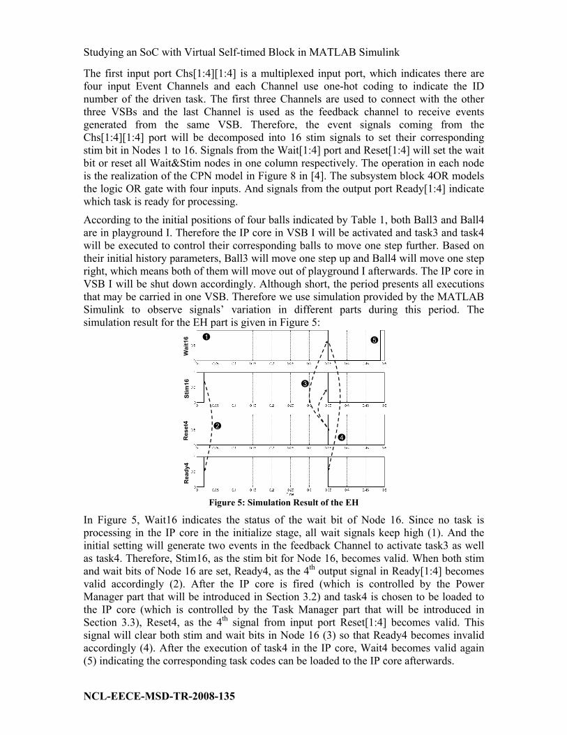
According to the initial positions of four balls indicated by Table 1, both Ball3 and Ball4

are in playground I. Therefore the IP core in VSB I will be activated and task3 and task4

will be executed to control their corresponding balls to move one step further. Based on

their initial history parameters, Ball3 will move one step up and Ball4 will move one step

right, which means both of them will move out of playground I afterwards. The IP core in

VSB I will be shut down accordingly. Although short, the period presents all executions

that may be carried in one VSB. Therefore we use simulation provided by the MATLAB

Simulink to observe signals’ variation in different parts during this period. The

simulation result for the EH part is given in Figure 5:

1

2

3

4

5

Wait16

Stim

16

Reset4

Ready4

Figure 5: Simulation Result of the EH

In Figure 5, Wait16 indicates the status of the wait bit of Node 16. Since no task is

processing in the IP core in the initialize stage, all wait signals keep high (1). And the

initial setting will generate two events in the feedback Channel to activate task3 as well

as task4. Therefore, Stim16, as the stim bit for Node 16, becomes valid. When both stim

and wait bits of Node 16 are set, Ready4, as the 4th output signal in Ready[1:4] becomes

valid accordingly (2). After the IP core is fired (which is controlled by the Power

Manager part that will be introduced in Section 3.2) and task4 is chosen to be loaded to

the IP core (which is controlled by the Task Manager part that will be introduced in

Section 3.3), Reset4, as the 4th signal from input port Reset[1:4] becomes valid. This

signal will clear both stim and wait bits in Node 16 (3) so that Ready4 becomes invalid

accordingly (4). After the execution of task4 in the IP core, Wait4 becomes valid again

(5) indicating the corresponding task codes can be loaded to the IP core afterwards.



3.2 The Design of Power Manager

Figure 6 is about the design of PM Part in a VSB which is the realization of the CPN

model of PM in Figure 9 in [4]. Each access subsystem block is the realization of the

corresponding access transition in the CPN model of Figure 9 in [4]. Each Polling block

is the realization of the corresponding select/pass transitions in Figure 9 in [4].

Figure 6: The Design of PM in MATLAB

The Trigger block in Figure 6 is based on the adder and Fire transitions in Figure 9 in [4].

Moreover, the weight of each task rather than the number of tasks is accumulated in this

block. Currently, fixed weight is given to each task and the realization of the trigger

block is given in Figure 7. If any grant signal from Grants[1:4] becomes valid, the

corresponding weight number from Weight[1:4] will be added to the accumulation data

which is kept in the Accumulation Memory block. Initially weight number 5 and 3 are

given to task3 and task4 respectively. Given Threshold 6, the accumulation of these two

tasks can active the IP core. A fire signal will be sent through the output port Fire

accordingly.

Figure 7: The Design of the Trigger Unit in Simulink

The simulation result of the PM part is given in Figure 8. The validation of Ready3 (as

the 3rd signal of Ready[1:4]) will disable Enable3 (as the enable signal for Ready3) so



that the corresponding weight can only be added once(1). Irdy3, as the output signal of

access3 in Figure 6 becomes valid accordingly (2). When at least one valid ready signal is

captured, the polling accumulation, which is introduced in Section 4.3, begins. When

Token3, as the 2nd input signal for Polling3 block, becomes valid, it indicates the polling

token arrives to check if Rdy3 is valid (3). Since Ready3 becomes valid earlier than

Token3, the former signal is granted. Therefore Grant3, as the 2nd output signal of

Polling3 block, becomes valid (4). The grant signal will lead the corresponding weight

for accumulation and Acc, as the accumulation result, increases to 5 (5). After the

accumulation in Acc, Irdy3 is withdrawn (6) and so is Grant3. The weight of task4 can be

added to the Acc afterwards in the similar executions. When the Acc becomes 8, the Fire

signal becomes valid accordingly (7). When the sleep signal becomes 0, both Enable3

and Enable4 becomes valid again to cooperate with further coming valid ready signals

(8).

1

2

3

4

5

7

6

Ready3

Ready4

8

Figure 8: The Simulation Result of the PM Part

3.3 The Design of Task Manager

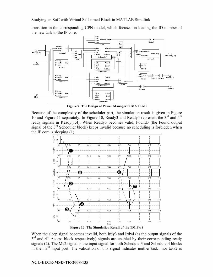
Figure 9 is about the design of the TM part in MATLAB which is the realization of the

CPN model of TM in Section 3.4.3 in [4]. Each Access subsystem block is the realization

of the corresponding Access transition in the CPN model in Figure 15 of [4]. Similarly

Each Scheduler block is the realization of the corresponding scheduling transition group

(combined by transitions Foundi, PollStarti, Passi, NextGi i=1,2,3,4) in the CPN model

of Figure 12 in [4]. Similarly as Figure 12 in [4], task1 and task2 have higher priority

than task3 and task4 in current model. Task1 and task3 are set as the initial last task in

each task group. The scheduling result will be given in the Found output port of each

scheduling block. And the block named Last in Figure 9 is one part of the realization of

the Load transition in Figure 15 of [4], which is used to update the information of the last

task in each group. The NewTask block is the other part of the realization of the Load



transition in the corresponding CPN model, which focuses on loading the ID number of

the new task to the IP core.

Figure 9: The Design of Power Manager in MATLAB

Because of the complexity of the scheduler part, the simulation result is given in Figure

10 and Figure 11 separately. In Figure 10, Ready3 and Ready4 represent the 3rd and 4

th

ready signals in Ready[1:4]. When Ready3 becomes valid, Found3 (the Found output

signal of the 3rd Scheduler block) keeps invalid because no scheduling is forbidden when

the IP core is sleeping (1).

1

2

3

4

5 6

7

LoadE

n

Figure 10: The Simulation Result of the TM Part

When the sleep signal becomes invalid, both Irdy3 and Irdy4 (as the output signals of the

3rd and 4

th Access block respectively) signals are enabled by their corresponding ready

signals (2). The Me2 signal is the input signal for both Scheduler3 and Scheduler4 blocks

in their 3rd input port. The validation of this signal indicates neither task1 nor task2 is



ready for execution. And this signal will enable Found4 (as Found output signal in the 4th

Scheduler Block) since Task3 is initially set as the last task (4). The scheduling result will

be loaded to the address bus and send to the IP core when the LoadEn signal becomes

valid (5) and the detail of task loading will be introduced in Figure 11. The loading of the

new task will also reset the corresponding ready signal in the EH part (which is

introduced in Section 3.1). When Ready4 becomes invalid, the Irdy4 becomes invalid

accordingly (6). Therefore Found3 becomes valid since Ready3 is the only valid ready

signal at this time (7).

Figure 11 focuses on executions in the TM part during the task loading processing. After

the scheduling result is achieved (1), NTask4, as the 4th signal of NewTask[1:4], becomes

1 when the LoadEn signal becomes valid (2). The LoadEn signal will be withdrawn when

task4 has been carried out in the IP core. The withdrawal of this signal will update the

record of last task in every priority group. In current case, Last4 becomes valid and Last3

becomes invalid at the same time because task4 is carried in the IP core (3). The

withdrawal of LoadEn will also trigger the Reset signal to update the record in the Event

Handler. In current case, a pulse of Reset4, as the 4th signal of Reset[1:4] is generated (4)

to clean the Stim&Wait bits in Node 13 to Node 16 of the EH part in Figure 4. This reset

operation will make Ready4 in Figure 10 invalid, and the change in ready signals triggers

another scheduling which choose task3 as the new candidate for IP core’s execution (5).

And this task will be chosen as the new task to the IP core when the next valid LoadEn

signal is issued (6).

1

2

3 4

5

6

LoadEn

Figure 11: The Simulation Result of Task Management (2)

3.4 The Design of Interface

Figure 12 is about the design of Interface part in MATLAB. The explanation of the

execution in this part can be found in the corresponding CPN model in Figure 12 in [4]

for detail.



The simulation result in this part is given in Figure 13. The validation of the Fire signal

from the A&F part will enable the wakeup signal to the IP core, given the IP core is

sleeping (1). Although the sleep signal from the IP core cannot be toggled because the

wakeup processing in the IP core just begins, the STEPSleep signal becomes 0 without

delay (2). This signal will disable the execution in the A&F part and enable scheduling in

the scheduler part, therefore the scheduling can be completed before the IP core

completes its wakeup processing. A LoadEn signal is issued afterwards (3). Tasks, as the

4th row in Figure 13, is the output of the 4OR block which is connected with

NewTask[1:4]. Therefore, when signal Tasks is 1, it means a non-zero task ID number is

loaded in the NewTask[1:4] (4).

Figure 12: The Design of Interface Part in Simulink

When the wakeup processing in the IP core is completed, the sleep signal becomes 0, and

a Read signal is generated accordingly (5) which will read the ID number of the new task

chosen from the STEP to the IP core. If the IP core starts execution the corresponding

task, the Current signal becomes valid (6), which will withdraw the LoadEn signal (7).

The following pulses in the Read signal are generated during the execution of the current

task in the IP core. When the current task is completed, the output control unit, which

will be introduced later in Figure 14 will decide which VSB will control the ball

movement corresponding to the current task. After the decision is made, a complete

signal will be issued, and this signal will trigger the issuing of another LoadEn signal (8).

According to Figure 2, both task3 and task4 can only be enabled once in VSB I because

their corresponding balls will move outside of playground I after one step. Therefore, the

3rd valid LoadEn signal cannot find any valid task ID number from the scheduler (9). In

this case, a Shutdown signal will be issued to IP core to start the shutdown processing

(10). At the same time, the STEPSleep signal becomes 1 to start operations in the A&F

part and disable operations in the scheduler part (11). However, the fire signal will only

wakeup the IP core again when the shutdown processing in the IP core is completed (12).



1

2

3

54

6

7

8

9

10

11

LoadE

n

12

Figure 13: The Simulation Result of the Interface Part

3.5 The Design of Output Control

Figure 14 is the design of the Output Control part in MATLAB Simulink. When the

current new position of one ball is calculated, its parameters will be loaded in the data

bus to be transferred to the ACM (which will be introduced in Section 4 for detail).

Therefore, the DeMux block is used to derive the PosX and PosY information from the

data bus. Two comparators are used to calculate which VSB will take charge of the ball

whose parameters are given in the data bus. When the decision is made, the ID number of

the ball (also the ID number of the corresponding task) in the Address[1:4] port will be

sent to the corresponding Output Channel (Ochi[1:4], i=0,1,2,3 and Och0[1:4] is the

feedback channel). At the same time, a Complete signal will be issued to the Interface

part to enable the next task loading.

Figure 14:The Design of Output Control Part in Simulink



Figure 15 is about the simulation result of this part. The Enable signal is the signal in the

first input port of both Comparator and Comparator1 blocks. EdgeX and EdgeY is the X

and Y position of the upper right edge of the current ball which is calculated in

Comparator and Comparator1 blocks. When the Enable signal becomes 1, the two

position parameters are used to decide which VSB will control the current ball (1).

2

3

1O

Ch1

OC

h2

Figure 15: The Simulation Result of the Output Control Part

Och1 in Figure 15 is the output signal of block 2And2 in Figure 14. The validation of this

signal indicates the current task will be sent out as an event from output channel 1 (2). At

the same time, the Complete signal becomes valid (1) to enable the Interface part to start

another task loading.

4. IP CORE DESIGN IN MATLAB SIMULINK

Figure 16 is about the design of the IP Core part in MATLAB Simulink. Two subsystem

blocks contains in this part. One is called OS which will take charge of wakeup/shutdown

the IP core according to the commands from the corresponding STEP. And it will load

new task ID number from the STEP. The block of Tasks is the combination of four

embedded tasks which is shown in Figure 17.

Figure 16: The Design of IP Core in Simulink

As introduced before, since we only care about the function of the IP core, five S-

functions are used in this part to realize both the OS block as well as the four tasks

embedded in this IP core. In Figure 17, four blocks Inputi (i=1,2,3,4) create input vectors

u for each task S-function. And similarly the four blocks Outputi (i=1,2,3,4) get output



vectors y from each task and turn them into signals that can be used in the other parts of

the MATLAB model. The four S-Function blocks name as Task i (i=1,2,3,4) are the

embedded codes for each task.

Figure 17: The Design of Task Subsystem Blocks in Simulink

4.1 Flow chart of the S-Function of OS

Start

Wakeup=1?

Sleep=1, Read=0

Wakeup processing

Complete?

Sleep=0, Read=1

Current=1?

Y

N

Y

N

N

Read=0

Current=0?

N

Y

Y

Shutdown=1?

Shutdown processing

Complete?

Read=0

N

Y

Y

N

Figure 18:The Flow Chart of the OS Program

Erreur ! Source du renvoi introuvable. provides the flow chart of the S-function code

for the OS program for VSB I. Initially when the program start, we suppose the IP core is



sleeping. Therefore, variables Sleep and Read in the output vector are set to 1 and 0

respectively. When the Wakeup signal from the input vector becomes 1, the OS starts the

wakeup processing. When the wakeup processing is completed, the Sleep signal is set to

0 so as to indicate the STEP that the IP core is ready for task processing. And the Read

signal is set to 1 so as to read new task from the STEP. If the IP core begins executing the

new task, the Current signal in the input vector will become 1, and it will set the Read

signal in the output vector to 0.

When the Current signal becomes 0, it means the current task is completed, and the Read

signal is set to 1 again to read new task from the STEP. This loop may continue several

times before the shutdown signal from the input vector is captured. In this case, the Read

signal will be first set to 0 since no new task will be read from the STEP, and the

shutdown processing begins. When the shutdown processing is completed, the Sleep

signal will be reset to 1 and the IP core starts sleeping until it is activated again.

4.2 Flow chart of the S-Function of TASK4

Figure 19 is about the flow chart of t he S-function code for task4 (since all task codes are

similar). The program starts when its ID number (for task4, [0 0 0 1]) is loaded in the

address bus. Signal Current in the output vector will be set to 1 so as to indicate the OS to

withdraw the Read signal. The first step of the task execution is to load parameter data of

all four balls from the ACM, which is carried out by the function DataLoad. With

parameters of the previous position of Ball4, task4 can calculate the next position of the

ball by the function NextPosition. This function will let the ball to move one step (the

size of the step is determined by the speed parameter) to the direction specified by the

History parameter.

Start

Current=1, i=0

DataLoad

Loading Complete?

UpdateHistory

N

Y

NextPosition

Collision(4,i)?

i<4?

i=i+1

Y

mod(History+1, 4)

N

Show the Ball

in New Position

Y

NDataTransfer

Transfer Complete?

Current=0

N

Y

Reset DataBus

End

Figure 19: The Flow Chart of the Task4 Program

Therefore, if the history parameter loaded from the ACM is used directly in the

NextPosition function, the new position calculated is totally determined by the current

position (unless Ball4 is knocked back by the wall of playground or collides with other

balls which will be discussed later). The UpdateHistory function (Figure 20) is used to

introduce some degree of nondeterministic to the ball moving.



0 1Threshold

NHistory=History NHistory=floor(unifrnd(0,4))

s=unifrnd(0,1) Figure 20: The Function of UpdateHistory

This function uses MATLAB command unifrnd to generate a random number from 0 to 1

which follows uniform distribution. If the random number is less than some Threshold

(0≤ Threshold ≤1), Task4 will use the history parameter loaded from the ACM to

generate the new ball position. Otherwise, a random integer number will be used to

generate the new ball position. Therefore, the bigger the Threshold value is, the more

deterministic the ball movement becomes. Otherwise, the ball movement becomes more

random. Different Threshold will be used for the analysis achieved in Section 5.

The loading of parameters for Ball4 from ACM is used for new position calculation, and

the loading of parameters of other three balls are used to check if the new position

calculated by the NextPosition function can have any collision with others. Function

Collision takes charge of the collision detection and Figure 21 indicates the mechanism

used by this function. The variable Dis_Centres calculate the distance between two balls’

centre. If Width1 and Width2 represent the width of the two balls separately, ball collision

happens when 22 )2

21(2_

WidthWidthCentresDis

+< .

2

2

2

212es)(Dis_Centr

+>

WidthWidth2

2

2

212es)(Dis_Centr

+≤

WidthWidth

CollisionNO Collision

Figure 21: The Calculation of Collision

Therefore in Figure 19, when the new position of ball4 is calculated, the program will

check if it has collision with other three balls in sequence (i in Figure 19 represents the

ball’s ID number). If any collision happens, the program will change the history

parameter and re-calculate the new position of Ball4 until no collision is found. After

collision detection, the program can safely show the ball in the new position, and then

transfer the parameters of Ball4 to the ACM. This data transfer is carried out by the

DataTransfer function. When the data transfer is completed, the task4 program reset the

Current signal to 0 so as to indicate the STEP to do output control, and the execution will

be stopped after the data bus is reset.

5. POWER AND LATENCY ANALYSIS

In our simulation, the time spent for one step movement of a ball without collision is set

as one time unit. Both wakeup and shutdown executions have been adjusted so that their

latency cost is one time unit as well. To simplify the analysis, we assume the power

dissipation for task processing is one unit and that for wakeup and shutdown is 1.5 units.

Because wire latency cannot be reflected by MATLAB Simulink, the time cost in a STEP



model cannot be compared with that in its IP core model. Therefore, the benchmark

achieved in this section takes the STEP as cost free in both power and latency.

With only four VSBs in the example SOC, events incoming to every VSB cannot be

taken as ideal exponential distribution. And with only four tasks embedded in every IP

core, the execution in every IP core cannot be taken as ideal exponential distribution

either. Therefore the example SOC test bench will be used to analyze the power

efficiency achieved by A&F policy in weak Markovian environment.

Four different DPM policies have been used to control the four VSBs in different tests.

The first one is greedy policy which means the threshold in the PM part is set to 1,

therefore any ball incoming to a black playground will activate the corresponding IP core.

A&F policy is used in our second simulation. As the priorities of the four balls have been

set as 1, 2, 3, 5 respectively, we set 5 as the threshold in every A&F part of STEP. It

means the incoming of ball4 only or several other balls to a black playground can activate

a sleeping IP core.

Timeout policy [6] serves as the third DPM policy in our test where we set the timeout

threshold to 5 and 10 time units in two different simulations.

Prediction policy is the fourth DPM policy that is implemented in our test. In [6], a TBE

time is defined as the minimum time spent in sleeping to compensate the wakeup and

shutdown overhead. In our case, the TBE is 3 time units. Furthermore, the implementation

of prediction policy needs to predict the length of next idle period according to [6].

Linear function is used in our test for idle period prediction (Equation 1).

321

_ *2.0*3.0*5.0 −−−

++=n

idle

n

idle

n

idle

n

predidle TTTT Equation 1

The prediction of the next (nth) idle period depends on the latest three idle periods with

reliability of 0.5, 0.3 and 0.2 respectively. For the implementation of Timeout or

Prediction policy, a subsystem block of state flow is used instead of the PM part in a

STEP.

To make our test have wide representation of real systems, we vary the threshold in

Figure 20 from 0 to 1 in 11 independent simulations for every DPM policy’s

implementation. The change of this threshold from 0 to 1 indicates the variation of ball

movements from pure random to mostly history based.

Figure 22 presents the average power dissipation of one IP core for various ball

movements when different DPM policies have been used. The Timeout1 in the legend

indicates the case when Timeout parameter τ is set to 5, and Timeout2 is the case when τ

is set to 10. From this figure, it is clear that A&F policy has the most power efficiency

that the other policies, no matter what movement balls take.



0

0.1

0.2

0.3

0.4

0.5

0.6

0.7

0.8

Pave

1 2 3 4 5 6 7 8 9 10 11

Threshold

Power Analysis

Series1

Series2

Series3

Series4

Series5

A&F

Greedy

Timeout1

Timeout2

Predict

0.9 0.8 0.7 0.6 0.5 0.4 0.3 0.2 0.1 0.0

Figure 22: Power Analysis of the example SoC

Figure 23 is about the latency analysis of the test bench when A&F policy is used. If four

tasks are ready in one IP core, 2 time units are needed by one task for scheduling before

execution in average, and 1 time unit is needed for execution at least (suppose no

collision happens). Therefore we set the deadline (DL) for every task’s execution as 6

time units in our first simulation. It can be seen front the figure that A&F policy causes

no more than 2.5% deadline violation in average. In most cases, this latency is

acceptable. In our second simulation, the deadline is set to 8 time units to present the case

when the deadline requirement is looser. It can be seen that the deadline violation

becomes less accordingly.

As different priorities have been given to the four tasks, these tasks have different latency

performance. Figure 24 presents the different latency performance of the four tasks when

the deadline is set to 6. It can be seen that task4, who has the highest priority, has extreme

low deadline violation cases. It is because no latency cost will be paid in task

accumulation.



0.018

0.019

0.02

0.021

0.022

0.023

0.024

0.025

APDV

1 2 3 4 5 6 7 8 9 10 11

Threshold

Latency

Series1

Series2

0.0 0.1 0.2 0.3 0.4 0.5 0.6 0.7 0.8 0.9 1.0

DL=6

DL=8

Figure 23: Latency Analysis of the example SoC

According to Figure 24, task2 and task3 have more frequent deadline violation than

task1, although they have higher priority than the latter. It is mainly caused by parameters

setting of these balls. According to Erreur ! Source du renvoi introuvable., ball2 and

ball3 have faster speed than ball1, which means ball2 or ball3 moves more frequently

across different playgrounds than ball1. When ball2 or ball3 moves to a new playground

whose corresponding IP core is sleeping, it needs another balls’ coming to activate the IP

core and much latency will be cost during task accumulation. On the other hand, ball1,

which has small size and slow speed, will always move within one playground. Therefore

this ball will pay less cost in accumulation latency than ball2 or ball3.

0

0.005

0.01

0.015

0.02

0.025

0.03

0.035

0.04

APDV

1 2 3 4 5 6 7 8 9 10 11

Threshold

APDV for different tasks

Series1

Series2

Series3

Series4

Task1

Task2

Task3

Task4

Figure 24: Latency Analysis of the example SoC (Continue)

6. CONCLUSION AND FUTURE WORK

This paper presents an example SoC which is constructed by four VSBs in MATLAB

Simulink. All parts of a STEP that are modelled by CPN models in [4], have been built

by basic components in Simulink Library. An example IP core with four embedded tasks



is designed in Simulink S-function. The example SOC is used to carry out a test bench

named as ball game in MATLAB simulation, and the simulation result achieved from the

test bench not only proves the correctness of executions in the VSB based SOC, but also

indicates the high energy efficiency of A&F policy even in a weak Markovian

environment.

The STEP model has also been implemented into VLSI design flow and benchmarks will

be achieved soon where the performance of the coprocessor is tested in real

implementation.

REFERENCES

[1] Yuan.Chen, Fei.Xia, Alex.Yakovlev, “Virtual Self-timed Block for Systems-

On-Chip”, ISCAS, 2006.

[2] Yuan Chen, Fei Xia, Delong Shang and Alex Yakovlev “Stochastic Modelling

Of Dynamic Power Management Policies And Analysis Of Their Power-

Latency Tradeoffs”, 4th UKEF, Southampton, 2008

[3] Yuan Chen, Fei Xia, Delong Shang and Alex Yakovlev “Fine Grain Stochastic

Modeling and Analysis of Low Power Portable Devices with Dynamic Power

Management”, 24th UKPEW, London, 2008

[4] Y Chen, F Xia, D Shang, A Yakovlev, “Virtual Self-timed Block Design using

Coloured Petri Nets”, NCL-EECE-MSD-TR-2008-134, Microelectronic

System Design Group, School of EECE, University of Newcastle upon Tyne,

Aug 2008

[5] F. Xia, and I. Clark, “Algorithms for Signal and message Asynchronous

Communication mechanisms and their Analysis,” in Fundamenta

Informaticae, Volume 50, Issue 2, 2002

[6] Y.Lu, E.Chung, T. Simunic, L. Benini, G. De Micheli “Quantitative

Comparison of Power Management Algorithms”, DATE 2000.

studying an soc with virtual self-timed blocks using

Documents