study regions - ars.els-cdn.com · web viewthe plain region is defined as the municipalities...

Supporting information to

Freshwater ecotoxicity impacts from pesticide use in

animal and vegetable foods produced in Sweden

Maria Nordborg,1 Jennifer Davis,2 Christel Cederberg,1 Anna Woodhouse 2

1 Department of Energy and Environment, Chalmers University of Technology, SE-412 96, Gothenburg, Sweden

2 SP Technical Research Institute of Sweden, Food and Bioscience, SE-402 29, Gothenburg, Sweden

CONTENTS

S1. Study regions.................................................................................................................2S2. Pesticide application data..............................................................................................3

S3. Field data (PestLCI).....................................................................................................11S4. Soil data (PestLCI).......................................................................................................12

S5. Climate data (PestLCI).................................................................................................14S6. Physico-chemical data of pesticide active substances (PestLCI)................................18

S7. Modeling of pesticide active substances......................................................................21S8. Pesticide active substances and characterization factors............................................23

S9. USEtox – additional information...................................................................................24S10. Physico-chemical data of pesticide active substances (USEtox).................................26

S11. Ecotoxicological effect data (USEtox)..........................................................................30S12. Expressing results in relation to different functional units............................................32

S13. Potential freshwater ecotoxicity impacts in crop production........................................34S14. Pesticide active substances with largest impact scores..............................................36

S15. Potential freshwater ecotoxicity impacts of broad beans.............................................37S16. Alternative soy-free feed rations for pigs and chickens: data and results....................38

S17. Pesticide active substances with largest emissions.....................................................40S18. Limitations....................................................................................................................41

References..............................................................................................................................42

Number of tables: 31

Number of figures: 4

Pages: 43

S1. Study regions

The plain region is defined as the municipalities Essunga, Grästorp, Gullspång, Götene, Lidköping,

Mariestad, Mellerud, Skara, Vara and Vänersborg, while the mixed landscape region is defined as all

other municipalities in the county of Västra Götaland, in line with the definition in Stenberg et al.

(2014). The plain and the mixed landscape regions correspond to the regions called “slättbygd” and

“mellanbygd”, respectively, in the “Paths to a sustainable food sector”-project (SLU, 2015).

S2. Pesticide application data

The pesticide application data (Tables S2.1 - S2.8) specify, for each application event, the type of

pesticide (herbicide, fungicide or insecticide), brand name of the pesticide product, active substance,

dose of pesticide product per application, active substance content in the pesticide product, frequency

of application, applied dose of active substance per application, average dose of active substance per

hectare and year, crop type and development stage (at time of application), method of application,

tillage type at time of application and application month. Frequency of application represents the share

of a field treated in a year, or the variation in treatment between years.

Crop types and development stages (at time of application) were determined for each application event

from a predefined list in PestLCI of over 100 available choices, based on the crop type, time of

application, assumed sowing time and information from SJV (2015a) and SJV (2015b).

Methods of application were determined for each application event from a predefined list of available

choices, including aircraft, soil incorporation and different tractor pulled booms. For each pesticide

application event, an appropriate boom type was determined with regard to the crop type, and

development stage at time of application.

Table S2.1 Pesticide application data for rapeseed, sown during the autumn (winter rapeseed). Data from rows 72-79 in tab "referens" in the Excel file "HBMV tid och bränsle för fältarbete samt pesticider HPPL" (Sonesson et al., 2014). Oilseed rape I = leaf development. Oilseed rape II = side shoots formation/stem elongation. H = herbicide. F = fungicide. I = insecticide. M = molluscicide.

Type Product Active substance

Dose of product (l ha-1 or kg ha-1)

AS content (g AS l-1 or g AS kg-1)

Application frequency (yr-1)

Calculated dose per application (kg AS ha-1)

Calculated yearly average (g AS ha-1 yr-1)

Crop type and development stage

Application method

Tillage type

Application month

H Butisan TopMetazachlor 2.00 375 1.0 0.750 750.0 Bare soil a Conv. boom

bare soil Conv. Sept.

Quinmerac 2.00 125 1.0 0.250 250.0 Bare soil a Conv. boom bare soil Conv. Sept.

F Cantus Boscalid 0.50 500 0.2 0.250 50.0 Oilseed rape I Conv. boom cereals Conv. Sept.

I Steward Indoxacarb 0.085 300 0.7 0.026 17.9 Oilseed rape II Conv. boom cereals Conv. April

M Sluxx b Ferric phosphate 5.50 30 0.4 - - - - - -

H Roundup Bio Glyphosate c 3.00 360 0.25 1.080 270.0 Bare soil d Conv. boom

bare soil Conv. Sept.a Applied after sowing, before plants develop.b Sluxx is excluded from the impact assessment due to USEtox being designed to handle primarily organic substances (ferric phosphate is an inorganic substance). The exclusion of this substance is not likely to significantly influence the results, since ferric phosphate occurs naturally in the soil and has very low toxicity to freshwater organisms (Buhl et al. 2013).c Addition to the original data, due to glyphosate being one of the most commonly used pesticides in Sweden (KemI, 2014). d Applied on stubble after harvest.

4

Table S2.2 Pesticide application data for feed wheat, sown during the autumn (winter wheat). Data from rows 24-31 in tab "referens" in the Excel file "HBMV tid och bränsle för fältarbete samt pesticider HPPL" (Sonesson et al., 2014). Cereals II = tillering. Cereals III = stem elongation. H = herbicide. F = fungicide. I = insecticide.








Application method

Tillage type

Application month

H Express 50 SX Tribenuron methyl 0.012 500 1.0 0.006 6.0 Cereals II Conv. boom

cereals Conv. May

H Starane 180 Fluroxypyr 0.60 180 1.0 0.108 108.0 Cereals II Conv. boom cereals Conv. May

F Sportak EW Prochloraz 1.00 450 0.05 0.450 22.5 Cereals III Conv. boom cereals Conv. June

F Comet Pyraclostrobin 0.30 250 0.7 0.075 52.5 Cereals III Conv. boom cereals Conv. June

F Proline EC 250 Prothioconazole 0.40 250 0.7 0.100 70.0 Cereals III Conv. boom

cereals Conv. June

I Mavrik 2F Tau fluvalinate 0.1625 240 0.3 0.039 11.7 Cereals III Conv. boom cereals Conv. July

H Roundup Bio Glyphosate a 3.00 360 0.25 1.080 270.0 Bare soil b Conv. boom bare soil Conv. Sept.

a Addition to the original data, due to glyphosate being one of the most commonly used pesticides in Sweden (KemI, 2014). b Applied on stubble after harvest.

5

Table S2.3 Pesticide application data for bread wheat, sown during the autumn (winter wheat). Data from rows 198-204 in tab "referens" in the Excel file "HBMV tid och bränsle för fältarbete samt pesticider HPPL" (Sonesson et al., 2014). Cereals II = tillering. Cereals III = stem elongation. H = herbicide. F = fungicide. I = insecticide.








Application method

Tillage type

Application month

H Express 50 SX Tribenuron methyl 0.012 500 1.0 0.006 6.0 Cereals II Conv. boom

cereals Conv. May

H Starane 180 Fluroxypyr 0.60 180 1.0 0.108 108.0 Cereals II Conv. boom cereals Conv. May

F Sportak EW Prochloraz 1.00 450 0.05 0.450 22.5 Cereals III Conv. boom cereals Conv. June

F Comet Pyraclostrobin 0.30 250 1.0 0.075 75.0 Cereals III Conv. boom cereals Conv. June

F Proline EC 250 Prothioconazole 0.40 250 1.0 0.100 100.0 Cereals III Conv. boom

cereals Conv. June

I Mavrik 2F Tau fluvalinate 0.1625 240 0.30 0.039 11.7 Cereals III Conv. boom cereals Conv. July



6

Table S2.4 Pesticide application data for barley, sown during the spring (spring barley). Data from rows 63-70 in tab "referens" in the Excel file "HBMV tid och bränsle för fältarbete samt pesticider HPPL" (Sonesson et al., 2014). Cereals I = leaf development. Cereals III = stem elongation. Cereals IV = booting/senescence. H = herbicide. F = fungicide. I = insecticide.



AS content (g AS l-1 org AS kg-1)





Application method

Tillage type

Application month

H Express 50 SX Tribenuron methyl 0.012 500 1.0 0.006 6.0 Cereals I Conv. boom

cereals Conv. May

F Comet Pyraclostrobin 0.25 250 0.6 0.063 37.5 Cereals III Conv. boom cereals Conv. July

F Stereo 312.5 EC

Cyprodinil 0.40 250 0.6 0.100 60.0 Cereals III Conv. boom cereals Conv. July

Propiconazole 0.40 62.5 0.6 0.025 15.0 Cereals III Conv. boom cereals Conv. July

I Karate 2,5 WP Lambda cyhalothrin 0.35 25 0.2 0.009 1.8 Cereals IV Conv. boom

cereals Conv. Aug.



Table S2.5 Pesticide application data for oats. Data from rows 15-22 in tab "referens" in the Excel file "HBMV tid och bränsle för fältarbete samt pesticider HPPL" (Sonesson et al., 2014). Cereals I = leaf development. Cereals II = tillering. Cereals III = stem elongation. H = herbicide. F = fungicide. I = insecticide.








Application method

Tillage type

Application month

H Express 50 SX Tribenuron methyl 0.012 500 1.0 0.006 6.0 Cereals I Conv. boom

cereals Conv. May

I Karate 2,5 WP Lambda cyhalothrin 0.35 25 0.2 0.009 1.8 Cereals II Conv. boom

cereals Conv. June

F Comet Pyraclostrobin 0.25 250 0.5 0.063 31.3 Cereals III Conv. boom cereals Conv. July


a Addition to the original data, due to glyphosate being one of the most commonly used pesticides in Sweden (KemI, 2014).b Applied on stubble after harvest.

7

Table S2.6 Pesticide application data for grass/clover. Data from rows 237-248 and rows 262-272 in tab "referens" in the Excel file "HBMV tid och bränsle för fältarbete samt pesticider HPPL" (Sonesson et al., 2014). H = herbicide.








Application method

Tillage type a

Application month

H Gratil 75 WG Amidosulfuron 0.05 750 0.17 b 0.038 6.25 Cereals I Conv. boom cereals No till May

H Roundup Bio Glyphosate 3.00 360 0.25 1.080 270.0 Grass I – all phases c

Conv. boom cereals Conv. Sept.

a No-till year 1 (ley succeeds the proceeding crop without tilling in between). Conventional tillage year 3, when the crop is removed. b 50% of the dose amidosulfuron has been allocated to grass/clover, and 50% to the cereal crop (typically oats or barley) in which the grass/clover-seed is sown. The dose allocated to grass/clover has been evenly distributed over the three years the grass/clover ley is established. c Applied on grass stubble after harvesting the final grass/clover silage in the third year.

Table S2.7 Pesticide application data for peas, determined based on information from the Swedish Board of Agriculture (SJV, 2015a, SJV, 2015b). Peas I = leaf development. Peas III = flowering/ripening. H = herbicide. I = insecticide.








Application method a

Tillage type

Application month

H Basagran SG Bentazone 0.60 870 1.0 0.522 522.0 Peas I Conv. boom cereals Conv. April

I Fastac 50 Alpha cypermethrin 0.30 50 0.3 0.015 7.5 Peas III Conv. boom cereals Conv. Aug.

H Roundup Bio Glyphosate 3.00 360 0.25 1.080 270.0 Bare soil b Conv. boom bare soil Conv. Sept.

a Cereals were considered most representative of peas, considering the available choices of pesticide application booms in PestLCI.b Applied on stubble after harvest.

8

Table S2.8 Pesticide application data for soybean. Data from the SB-I case (soybean that is not genetically engineered to tolerate glyphosate) in Nordborg et al. (2014), which in turn were obtained from a conventional farmer in Mato Grosso, Brazil, through the Mato Grosso State Soy and Corn Producers Association, APROSOJA. Data have been reviewed, and slightly modified, by D. Meyer (pers. comm. 2013). Soybean I = leaf/ harvestable plant parts development. Soybean II = side shoot and harvestable part development. Soybean III = inflorescence emergence/senescence. H = herbicide. F = fungicide. I = insecticide.








Application method a

Tillage type

Application month

H Gromoxone Paraquat 1.50 200 1.0 0.300 300.0 Bare soil Conv. boom bare soil No till Sept.

H Drible Lactofen 0.30 240 1.0 0.072 72.0 Soybean I Conv. boom potato No till Oct.

I Fastac Alpha cypermethrin 0.30 100 1.0 0.030 30.0 Soybean I Conv. boom potato No till Oct.

I Lannate Methomyl 0.70 215 1.0 0.151 150.5 Soybean I Conv. boom potato No till Oct.

H Basagran Bentazone 0.90 600 1.0 0.540 540.0 Soybean I Conv. boom potato No till Oct.

H Naja Lactofen 0.25 240 1.0 0.060 60.0 Soybean I Conv. boom potato No till Oct.

H Classic Chlorimuron ethyl 0.04 250 1.0 0.010 10.0 Soybean I Conv. boom potato No till Oct.

I Premio Chlorantraniliprole 0.025 200 1.0 0.005 5.0 Soybean I Conv. boom potato No till Oct.

H Select Clethodim 0.35 240 1.0 0.084 84.0 Soybean I Conv. boom potato No till Nov.

F Comet Pyraclostrobin 0.30 250 1.0 0.075 75.0 Soybean I Conv. boom potato No till Nov.

I Premio Chlorantraniliprole 0.025 200 1.0 0.005 5.0 Soybean I Conv. boom potato No till Nov.

F OperaPyraclostrobin 0.50 133 1.0 0.067 66.5 Soybean II Conv. boom

potato No till Nov.

Epoxiconazole 0.50 50 1.0 0.025 25.0 Soybean II Conv. boom potato No till Nov.

I Premio Chlorantraniliprole 0.05 200 1.0 0.010 10.0 Soybean II Conv. boom potato No till Nov.

F OperaPyraclostrobin 0.50 133 1.0 0.067 66.5 Soybean II Conv. boom

potato No till Dec.

Epoxiconazole 0.50 50 1.0 0.025 25.0 Soybean II Conv. boom potato No till Dec.

I Nomolt Teflubenzuron 0.15 150 1.0 0.023 22.5 Soybean II Conv. boom No till Dec.

9

potato

I Platinum Neo

Thiamethoxam 0.30 141 1.0 0.042 42.3 Soybean III Conv. boom potato No till Jan.

Lambda cyhalothrin 0.30 106 1.0 0.032 31.8 Soybean III Conv. boom potato No till Jan.

H Gromoxone Paraquat 1.50 200 1.0 0.300 300.0 Soybean III Conv. boom potato No till Feb.

a The potato plant was considered most representative of the soybean plant, based on the selection of available boom types in PestLCI (a different boom was used in Nordborg et al. 2014).

10

S3. Field data (PestLCI)

PestLCI takes into account the following field parameters: field size (length and width), slope, fraction

drained, depth of drainage system and irrigation. For the regions in Västra Götaland, these parameters

were set based on information in Sonesson et al., (2014), and own assumptions. For Mato Grosso,

Brazil, field data were set as in Nordborg et al. (2014). For consistency in modeling, we assumed that

all fields were of the same shape (quadratic).

PestLCI also enables the modeling of buffer zones, i.e., safety areas between field and surface waters

where pesticides are not sprayed. We assumed that buffer zones were not used (i.e., set to 0 m, which

is the default option in PestLCI).

Table S3.1 Field data used in the pesticide emission inventory.

Region Field size (ha), width×length (m) a Slope (%) Fraction

drained (%) b

Depth of drainage system (m) b

Annual irrigation (mm) c

Mixed landscape region in Västra Götaland, Sweden 5 d, 224×224 2.7 e 0 not applicable 0

Plain region in Västra Götaland, Sweden. 13 d, 361×361 0 f 0 not applicable 0

Mato Grosso, Brazil g 250, 1581×1581 1 0 not applicable 0a Field width and length were set based on the assumption that all fields are quadratic in shape.b We did not consider drainage, since drainage systems are often installed below 1 m depth, while the soil in PestLCI is only modelled down to a depth of 1 m. c None of the crops were assumed to be irrigated in line with dominant cultivation practices in the studied regions.d Data from Table 7 in Stenberg et al. (2014).e Data from a digital elevation model (Jarvis et al. 2008), derived using ArcGIS, representing the average slope on cropland in Västra Götaland. f Own assumption.g We used the same data to represent fields in Mato Grosso, Brazil, as used in Nordborg et al. (2014), except that we assumed quadratic fields here, resulting in different width and length.

11

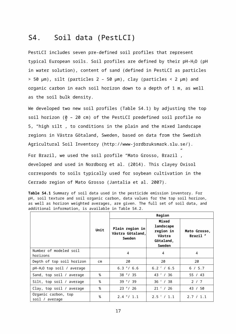
S4. Soil data (PestLCI)

PestLCI includes seven pre-defined soil profiles that represent typical European soils. Soil profiles are

defined by their pH-H2O (pH in water solution), content of sand (defined in PestLCI as particles > 50

μm), silt (particles 2 – 50 μm), clay (particles < 2 μm) and organic carbon in each soil horizon down to

a depth of 1 m, as well as the soil bulk density.

We developed two new soil profiles (Table S4.1) by adjusting the top soil horizon (0 – 20 cm) of the

PestLCI predefined soil profile no 5, “high silt”, to conditions in the plain and the mixed landscape

regions in Västra Götaland, Sweden, based on data from the Swedish Agricultural Soil Inventory

(http://www-jordbruksmark.slu.se/).

For Brazil, we used the soil profile “Mato Grosso, Brazil”, developed and used in Nordborg et al.

(2014). This clayey Oxisol corresponds to soils typically used for soybean cultivation in the Cerrado

region of Mato Grosso (Jantalia et al. 2007).

Table S4.1 Summary of soil data used in the pesticide emission inventory. For pH, soil texture and soil organic carbon, data values for the top soil horizon, as well as horizon weighted averages, are given. The full set of soil data, and additional information, is available in Table S4.2.

Unit

Region

Plain region in Västra Götaland, Sweden

Mixed landscape region in Västra

Götaland, Sweden

Mato Grosso, Brazil d

Number of modeled soil horizons 4 4 4

Depth of top soil horizon cm 20 20 20

pH-H2O top soil / average 6.3 a / 6.6 6.2 c / 6.5 6 / 5.7

Sand, top soil / average % 38 a / 35 43 c / 36 55 / 43

Silt, top soil / average % 39 a / 39 36 c / 38 2 / 7

Clay, top soil / average % 23 a / 26 21 c / 26 43 / 50

Organic carbon, top soil / average % 2.4 a / 1.1 2.5 c / 1.1 2.7 / 1.1

Soil bulk density kg m-3 1433 b 1433 b 1350a Top soil conditions in the plain region were set based on average conditions in the predefined region “Vänerslätten”, available in the Swedish Agricultural Soil Inventory (http://www-jordbruksmark.slu.se/, accessed June 30, 2015). Averages were used throughout, except organic carbon, where the median was used, in order to avoid that organic soils shift the average upwards. Data values are based on a total of 661 soil samples for sand, silt and clay, and 679 soil samples for pH and organic carbon, taken between 1988 and 2007. The clay content on the plain corresponds fairly well to the value of 24% for “slättbygd”, given in Table 7 in Stenberg et al. (2014).b We used the same value for soil bulk density as used in the PestLCI predefined soil profile no 5 “high silt”.c Top soil conditions in the mixed landscape region were set based on average conditions in the county “Västra Götaland” (including the municipalities defined as the plain, due to lack of a more appropriate predefined region). Data were derived from the Swedish Agricultural Soil Inventory (http://www-jordbruksmark.slu.se/, accessed June 30, 2015) and are based on a total of 880 soil samples for sand, silt and clay, 905 soil samples for pH and 906 soil samples for organic carbon, taken between 1988 and 2007. Averages were used throughout, except organic carbon, where the median was used, in order to avoid that organic soils shift the average upwards. The clay content in the mixed landscape region corresponds fairly well to the value of 19% for “mellanbygd”, given in Table 7 in Stenberg et al. (2014).d For Mato Grosso, Brazil, we used the soil profile “Mato Grosso, Brazil”, developed and used in Nordborg et al. (2014).

12

http://www-jordbruksmark.slu.se/

http://www-jordbruksmark.slu.se/

Table S4.2 The full soil data sets for the three studied regions. Data sources are given in Table S4.1. Plain region in Västra Götaland, Sweden

Mixed landscape region in Västra Götaland, Sweden

Mato Grosso, Brazil

start layer 1 (m) 0 0 0start layer 2 (m) 0.20 0.20 0.20start layer 3 (m) 0.65 0.65 0.40start layer 4 (m) 0.95 0.95 0.60start layer 5 (m) 1.0 1.0 1.0pH layer 1 6.31 6.20 6.00pH layer 2 6.40 6.40 5.30pH layer 3 6.90 6.90 5.60pH layer 4 7.10 7.10 5.70f(clay) layer 1 0.229 0.207 0.430f(silt) layer 1 0.393 0.364 0.020f(sand) layer 1 0.378 0.429 0.550f(clay) layer 2 0.270 0.270 0.490f(silt) layer 2 0.388 0.388 0.100f(sand) layer 2 0.341 0.341 0.410f(clay) layer 3 0.281 0.281 0.540f(silt) layer 3 0.386 0.386 0.070f(sand) layer 3 0.333 0.333 0.390f(clay) layer 4 0.250 0.250 0.530f(silt) layer 4 0.415 0.415 0.080f(sand) layer 4 0.335 0.335 0.390f(OC) layer 1 % 2.36 2.52 2.70f(OC) layer 2 % 0.90 0.90 1.00f(OC) layer 3 % 0.60 0.60 0.70f(OC) layer 4 % 0.30 0.30 0.50Soil bulk density 1433 1433 1350

Different definitions of particle sizes exist for the clay, silt and sand particles of the soil. The

definitions that PestLCI and the Swedish Agricultural Soil Inventory use differ slightly for sand and

silt, while they match for clay (Table S4.3). We did not adjust for these differences, which were

considered minor and not likely to significantly influence results.

Table S4.3 Particle size definitions of the fine earth fraction of the soil (particles < 2 mm) according to PestLCI and the Swedish Agricultural Soil Inventory (http://www-jordbruksmark.slu.se/).

Clay Silt Sand

PestLCI < 2 μm 2 – 50 μm > 50 μm

Swedish Agricultural Soil Inventory < 2 μm a 2 – 60 μm b > 60 μm c

a “Ler_<0,002mm” in the Swedish Agricultural Soil Inventory.b “Silt_0,06-0,002mm” in the Swedish Agricultural Soil Inventory.c “Sand_2-0,06mm” in the Swedish Agricultural Soil Inventory.

13

S5. Climate data (PestLCI)

PestLCI includes 25 pre-defined climate profiles that represent climate conditions throughout Europe.

Climate profiles are defined by the location’s average, maximum and minimum air temperatures,

precipitation, number of days with rainfall, solar radiation, annual average potential evaporation, and

elevation above sea level.

We developed one new climate profile (Table S5.1), to account for conditions in Västra Götaland.

This climate profile was used to represent climate conditions both in the plain, and in the mixed

landscape region, in Västra Götaland. For Brazil, we used the climate profile “Mato Grosso, Brazil”,

developed and used in Nordborg et al. (2014).

Table S5.1 Summary of climate data used in the pesticide emission inventory. The municipality of Vara was considered in the parameterization of the climate profile for Västra Götaland. The full set of climate data, and additional information, is available in Table S5.2.

UnitRegion

Västra Götaland, Sweden

Mato Grosso, Brazil a

Elevation above sea level m 80 b 400

Average air temperature, yearly average °C 6.1 c 25.2

Average minimum air temperature, yearly average °C 2.3 c 19.5

Average maximum air temperature, yearly average °C 9.9 c 32.6

Annual total rainfall mm 590 d 1620

Rain days ( > 1 mm), monthly average - 8.4 e 13.6

Annual potential evaporation mm 593 f 1425

Solar radiation, yearly average Wh m-2 day-1 2710 g 5290a For Mato Grosso, Brazil, we used the climate profile “Mato Grosso, Brazil”, developed and used in Nordborg et al. (2014).b Data from Altitude Website http://altitude.nu/ (accessed June 23, 2015).c Data from visual inspection of color coded maps at http://www.smhi.se/klimatdata/meteorologi/temperatur/ (accessed June 24, 2015), representing average monthly average/minimum/maximum air temperatures for the Weather Normal Period 1961 – 1990.d Data from visual inspection of color coded maps at http://www.smhi.se/klimatdata/meteorologi/nederbord/ (accessed June 24, 2015), representing average monthly rainfall for the Weather Normal Period 1961 – 1990.e Data from the climate profile “Linköping, Sweden” developed and used in Nordborg et al. (2014), assuming similar conditions in Vara, as in Linköping, based on a map showing the yearly average days with > 1 mm precipitation, available at http://www.smhi.se/klimatdata/meteorologi/nederbord (accessed June 24, 2015).f Data from the climate profile “Linköping, Sweden” developed and used in Nordborg et al. (2014), assuming similar conditions in Vara, as in Linköping.g Data from the National Renewable Energy Laboratory’s (NREL) PVWatts Calculator http://pvwatts.nrel.gov/ (accessed June, 24 2015), representing solar radiation in Vara on a horizontal plane.

14

Table S5.2 The full climate data sets for the studied regions. The municipality of Vara was considered in the parameterization of the climate profile for Västra Götaland. Data sources are given in Table S5.1. The climate data set include two derived parameters that are calculated based on the collected data: average rainfall on a rainy day (calculated as average monthly precipitation divided by number of days with >1 mm precipitation) and rain frequency (calculated as number of days in the month divided by number of days with >1 mm precipitation).

Västra Götaland, Sweden Mato Grosso, Brazil

Latitude (degrees) 58.26 N 14.24 S Longitude (degrees. E+ W-) 12.98 E 56.27 WElevation (m) 80.0 400.0TG jan (degC) -3.0 24.0TG feb (degC) -3.0 27.0TG mar (degC) -0.5 24.3TG apr (degC) 4.5 27.7TG may (degC) 10.5 24.4TG jun (degC) 14.5 25.4TG jul (degC) 15.5 24.5TG aug (degC) 15.0 24.7TG sept (degC) 11.0 25.3TG oct (degC) 7.0 24.5TG nov (degC) 2.0 25.0TG dec (degC) -1.0 25.5TG average (degC) 6.1 25.2TMIN jan (degC) -6.0 20.4TMIN feb (degC) -6.0 21.2TMIN mar (degC) -3.5 20.4TMIN apr (degC) 0.5 20.4TMIN may (degC) 5.0 19.1TMIN jun (degC) 9.0 15.1TMIN jul (degC) 11.0 16.4TMIN aug (degC) 10.0 19.1TMIN sept (degC) 7.0 19.5TMIN oct (degC) 4.0 20.8TMIN nov (degC) -0.5 21.8TMIN dec (degC) -4.0 19.9TMIN average (degC) 2.3 19.5TMAX jan (degC) -0.5 32.3TMAX feb (degC) -0.5 31.6TMAX mar (degC) 3.5 31.4TMAX apr (degC) 8.5 33.6TMAX may (degC) 15.5 31.5TMAX jun (degC) 19.5 32.1TMAX jul (degC) 20.5 32.8TMAX aug (degC) 19.5 34.9TMAX sept (degC) 15.5 32.5TMAX oct (degC) 10.5 32.2TMAX nov (degC) 5.0 32.9TMAX dec (degC) 1.0 32.9TMAX average (degC) 9.9 32.6

15

Rainfall Jan (mm) 40.0 268.1Rainfall Feb (mm) 25.0 235.5Rainfall Mar (mm) 35.0 203.4Rainfall Apr (mm) 35.0 137.8Rainfall May (mm) 45.0 55.5Rainfall Jun (mm) 50.0 9.5Rainfall Jul (mm) 65.0 6.9Rainfall Aug (mm) 65.0 27.3Rainfall Sep (mm) 65.0 72.2Rainfall Oct (mm) 65.0 151.1Rainfall Nov (mm) 55.0 204.5Rainfall Dec (mm) 45.0 248.0Total rainfall year (mm) 590.0 1619.8Rain days (>1mm) Jan 7.9 24.0Rain days (>1mm) Feb 7.2 20.0Rain days (>1mm) Mar 6.3 22.0Rain days (>1mm) Apr 7.2 16.0Rain days (>1mm) May (mm) 6.9 8.0Rain days (>1mm) Jun (mm) 10.8 3.0Rain days (>1mm) Jul (mm) 8.5 2.0Rain days (>1mm) Aug (mm) 9.3 3.0Rain days (>1mm) Sep (mm) 9.0 7.0Rain days (>1mm) Oct (mm) 8.3 16.0Rain days (>1mm) Nov (mm) 10.1 20.0Rain days (>1mm) Dec (mm) 8.9 23.0Rain days (>1mm) Average (mm) 8.4 13.6Average rainfall on rainy day Jan (mm) 5.1 11.2Average rainfall on rainy day Feb (mm) 3.5 11.8Average rainfall on rainy day Mar (mm) 5.6 9.2Average rainfall on rainy day Apr (mm) 4.9 8.6Average rainfall on rainy day May (mm) 6.5 6.9Average rainfall on rainy day Jun (mm) 4.6 3.2Average rainfall on rainy day Jul (mm) 7.6 3.5Average rainfall on rainy day Aug (mm) 7.0 9.1Average rainfall on rainy day Sep (mm) 7.2 10.3Average rainfall on rainy day Oct (mm) 7.8 9.4Average rainfall on rainy day Nov (mm) 5.4 10.2Average rainfall on rainy day Dec (mm) 5.1 10.8Average rainfall on rainy day Average (mm) 5.9 8.7Rain frequency Jan (day-1) 3.9 1.3Rain frequency Feb (day-1) 3.9 1.4Rain frequency Mar (day-1) 4.9 1.4Rain frequency Apr (day-1) 4.2 1.9Rain frequency May (day-1) 4.5 3.9Rain frequency Jun (day-1) 2.8 10.0Rain frequency Jul (day-1) 3.6 15.5Rain frequency Aug (day-1) 3.3 10.3Rain frequency Sep (day-1) 3.3 4.3Rain frequency Oct (day-1) 3.7 1.9

16

Rain frequency Nov (day-1) 3.0 1.5Rain frequency Dec (day-1) 3.5 1.3Rain frequency Average (day-1) 3.7 4.6Annual potential evaporation (mm) 593 1426Solar irradiation Jan (Wh m-2 day-1) 340 5920Solar irradiation Feb (Wh m-2 day-1) 840 5175Solar irradiation Mar (Wh m-2 day-1) 2060 5140Solar irradiation Apr (Wh m-2 day-1) 3690 5340Solar irradiation May (Wh m-2 day-1) 5370 5039Solar irradiation Jun (Wh m-2 day-1) 5450 3969Solar irradiation Jul (Wh m-2 day-1) 5460 4441Solar irradiation Aug (Wh m-2 day-1) 4180 5351Solar irradiation Sep (Wh m-2 day-1) 2820 5807Solar irradiation Oct (Wh m-2 day-1) 1420 6003Solar irradiation Nov (Wh m-2 day-1) 500 5820Solar irradiation Dec (Wh m-2 day-1) 260 5484Solar irradiation Average (Wh m-2 day-1) 2710 5292

17

S6. Physico-chemical data of pesticide active substances (PestLCI)

Table S7.1 Physico-chemical parameters of pesticides used in PestLCI. The full set of physico-chemical data that was used here is available in Table S7.2. For more information about PestLCI, refer to Birkved and Hauschild (2006) and Dijkman et al (2012).

Parameter Unit Explanation

Type - Herbicide, insecticide, fungicide, etc.

CAS-RN - Chemical Abstracts Service Registry Number.

SMILES - Simplified Molecular Input Line Entry System-notation.

Molecular weight g mole-1 Also called molecular mass.

Molecular volume cm3 mole-1 Calculated based on molecular weight and bulk density.

Solubility, ref. temp. g l-1, oC Solubility in water and reference temperature at which it was determined.

Vapor pressure, ref. temp. Pa, oC Vapor pressure and reference temperature at which it was determined.

pKa - First dissociation constant (neutral to charged). Not applicable for non-ionizing substances.

log Kow - Log of partitioning coefficient between octanol and water

Koc l kg-1 Partitioning coefficient between soil organic carbon and water

Soil t½, ref. temp. days, oC Soil aeraobic biodegradation half-life “DT50 (lab at 20°C)” and temperature at which it was determined.

Atmospheric OH rate cm3

molecule-1 s-1 Overall OH-radical oxidation rate constant.

Bufferzone width m Width of the zone along the edges of the field in which it is forbidden to spray the chemical (default = 0 m).

E(a) Evaporation kJ mole-1 Activation energy for evaporation. We used the default value of 100 kJ mole-1.

18

Table S7.2 Full set of physico-chemical data used in PestLCI. Pesticide active substances that were not originally included in the PestLCI v.2.0 database, but that were added in Nordborg et al. (2014), are marked with †. For more information about data sources, refer to Nordborg et al. (2014). Notations as in PestLCI. The table continues on the next page.

Pesticide active substance

Molecular weight, g mole-1

Molecular volume, cm3 mole-1

Solubility in water, g l-1

Ref. temp. solubility, oC

Vapour pressure, Pa

Ref. temp Vap. pr., oC

Alpha cypermethrin (I) 416.3 313.1 4.00E-6 20 3.4E-7 25Amidosulfuron (H) 369.4 231.6 3.07E-0 20 1.3E-5 25Bentazone (H) 240.3 178.5 0.57E-0 20 1.7E-4 25Boscalid (F) † 343.2 194.4 4.60E-3 20 7.2E-7 25Chlorantraniliprole (I) † 483.2 320.0 8.80E-4 20 6.3E-12 25Chlorimuron ethyl (H) † 414.8 277.7 1.20E-0 20 4.9E-10 25Clethodim (H) † 359.9 312.4 5.45E-0 20 2.1E-6 25Cyprodinil (F) 225.3 186.1 1.30E-2 20 5.1E-4 25Epoxiconazole (F) † 329.8 236.4 7.10E-3 20 1.0E-5 25Fluroxypyr (H) 255.0 234.0 6.50E-0 20 3.8E-9 25Glyphosate (H) 169.1 100.6 10.5E-0 20 1.3E-5 25Indoxacarb (I) 527.8 366.5 2.00E-4 20 6.0E-6 25Lactofen (H) † 461.8 341.6 5.00E-4 20 9.3E-6 25Lambda cyhalothrin (I) 449.9 334.6 5.00E-6 20 2.0E-7 25Metazachlor (H) 277.8 232.1 0.45E-0 20 9.3E-5 25Methomyl (I) 162.2 137.9 55.0E-0 20 7.2E-4 25Paraquat (H) † 186.3 124.2 620E-0 20 1.0E-5 25Prochloraz (F) 376.7 274.2 2.65E-2 20 1.5E-4 25Propiconazole (F) 342.2 244.8 0.15E-0 20 5.6E-5 25Prothioconazole (F) † 344.3 228.0 0.30E-0 20 4.0E-7 25Pyraclostrobin (F) † 387.8 303.4 1.90E-3 20 2.6E-8 25Quinmerac (H) † 221.6 157.5 107E-0 20 1.0E-10 25Tau fluvalinate (I) 502.9 383.0 1.03E-6 20 9.0E-11 25Teflubenzuron (I) † 381.1 231.4 1.00E-5 20 9.2E-7 25Thiamethoxam (I) 291.7 170.2 4.10E-0 20 6.6E-9 25Tribenuron methyl (H) 395.4 277.3 2.04E-0 20 5.3E-8 25

19

Table S7.2 Continued Full set of physico-chemical data used in PestLCI. Pesticide active substances that were not originally included in the PestLCI v.2.0 database, but that were added in Nordborg et al. (2014), are marked with †. For more information about data sources, refer to Nordborg et al. (2014). Notations as in PestLCI.

Pesticide active substance pKa (first), -

Log Kow, -

Koc, l kg-1

Soil t½ Lab 20° C, days

Ref. temp biodegr., oC

Atmospheric OH rate

(days) at 25° C, cm3 molecule-1 s-1

Alpha cypermethrin (I) 5.00 5.50 57900 100 20 2.14E-11Amidosulfuron (H) 3.58 -1.56 29.3 17 20 2.05E-10Bentazone (H) 3.28 -0.46 5.3 45 20 6.22E-11Boscalid (F) † 'N/A' 2.96 1225 246 20 2.60E-11Chlorantraniliprole (I) † 10.88 2.86 362 597 20 1.67E-11Chlorimuron ethyl (H) † 4.20 0.11 106 40 20 4.27E-11Clethodim (H) † 4.47 4.14 150000 0.55 20 1.55E-10Cyprodinil (F) 4.44 4.00 2277 53 20 2.00E-10Epoxiconazole (F) † 'N/A' 3.30 1073 226 20 8.78E-12Fluroxypyr (H) 2.94 0.04 195 13 20 2.88E-11Glyphosate (H) 2.34 -3.20 1435 49 20 7.90E-11Indoxacarb (I) 'N/A' 4.65 6450 5 20 4.17E-11Lactofen (H) † 'N/A' 4.81 10000 4 20 3.21E-12Lambda cyhalothrin (I) 'N/A' 5.50 284000 175 20 3.15E-11Metazachlor (H) 'N/A' 2.49 54 10.8 20 5.90E-11Methomyl (I) 'N/A' 0.09 72 7 20 6.65E-12Paraquat (H) † 'N/A' -4.50 1000000 5000 20 2.16E-11Prochloraz (F) 3.80 3.50 500 224 20 7.80E-11Propiconazole (F) 1.09 3.72 1086 90 20 2.32E-11Prothioconazole (F) † 6.90 3.82 1765 0.5 20 1.13E-10Pyraclostrobin (F) † 'N/A' 3.99 9304 62 20 2.06E-10Quinmerac (H) † 4.31 -1.41 86 17 20 4.37E-12Tau fluvalinate (I) 'N/A' 7.02 135000 31 20 2.93E-11Teflubenzuron (I) † 9.20 4.30 26100 92 20 6.19E-12Thiamethoxam (I) 'N/A' -0.13 56.2 121 20 2.49E-10Tribenuron methyl (H) 4.70 0.78 35 14 20 2.96E-12

20

S7. Modeling of pesticide active substances

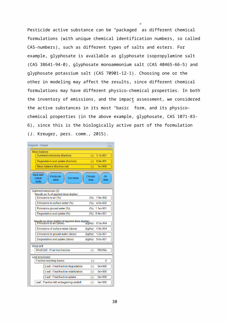
To calculate the emissions from the use of glyphosate in rapeseed, we selected glyphosate in the

PestLCI model, entered the dose per application (1.08 kg ha-1 of active substance, see Table S2.1), and

adjusted all model parameters (month, soil, climate, method of application etc.) to conditions in the

plain region of Västra Götaland, Sweden (see Tables S3.1, S4.1 and S5.1). A screenshot of the model

set up for this calculation is presented in Figure S7.1. As a result, PestLCI returned the emissions to air

and surface water: 8.5E-04 and 4.9E-04 kg ha-1, respectively, see Figure 7.2

Figure 7.1 Screenshot of the PestLCI model set up for calculating the emissions from the use of glyphosate in rapeseed (the soil profile in the plain region is called slättbygd in the model, which is Swedish for plains).

Pesticide active substance can be “packaged” as different chemical formulations (with unique

chemical identification numbers, so called CAS-numbers), such as different types of salts and esters.

For example, glyphosate is available as glyphosate isopropylamine salt (CAS 38641-94-0), glyphosate

monoammonium salt (CAS 40465-66-5) and glyphosate potassium salt (CAS 70901-12-1). Choosing

one or the other in modeling may affect the results, since different chemical formulations may have

different physico-chemical properties. In both the inventory of emissions, and the impact assessment,

we considered the active substances in its most “basic” form, and its physico-chemical properties (in

21

the above example, glyphosate, CAS 1071-83-6), since this is the biologically active part of the

formulation (J. Kreuger, pers. comm., 2015).

Figure 7.2 Screenshot of the resulting output from the PestLCI model: emissions to air and surface water from the use of glyphosate in rapeseed.

Only the pesticide ingredients listed as active substances in the Swedish Chemical Agency’s pesticide

database (KemI, 2015) are included. For some products (e.g., Comet used in the cultivation of wheat,

barley, oats and soybean), discrepancies exist regarding which ingredients are considered active,

between information available from producers, and information available in the Swedish Chemical

Agency’s pesticide database (KemI, 2015).

Other ingredients in pesticide products, such as solvents and surfactants, are not included.

22

S8. Pesticide active substances and characterization factors

Table S8.1 Pesticide active substances included in this study, and their Chemical Abstracts Service Registry Numbers (CAS-RN), characterization factors for emissions to continental air and continental freshwater, and characterization factor classification. Active substances that were not originally included in the PestLCI v.2.0 database, but that were added in Nordborg et al. (2014), are marked with † (no new active substances were added to PestLCI in this study). Pesticide active substances that did not originally have USEtox 2.01 characterization factors, but that were calculated here, are marked with *. Active substances marked with ǂ were included in the USEtox 2.01 database, but had their physico-chemical, and for teflubenzuron and alpha cypermethrin, also their ecotoxicological input data, reviewed, and updated, if judged necessary (for more information see Chapter S10 and S11). H = herbicide, F = fungicide, I = insecticide.

CAS-RN Pesticide active substance

Characterization factors for emission to air (CTUe kg-1)

Characterization factors for emission to freshwater (CTUe kg-1)

Characterization factor classification

67375-30-8 Alpha cypermethrin (I) ǂ 66 828 11 154 613 Recommended a

120923-37-7 Amidosulfuron (H) * 19 1 689 Recommended25057-89-0 Bentazone (H) 3 200 Recommended188425-85-6 Boscalid (F) * † 1 121 15 949 Indicative b

500008-45-7 Chlorantraniliprole (I) * † 25 072 89 462 Recommended90982-32-4 Chlorimuron ethyl (H) * † 646 16 565 Recommended99129-21-2 Clethodim (H) † 11 3 663 Recommended121552-61-2 Cyprodinil (F) 60 28 049 Recommended135319-73-2 Epoxiconazole (F) * † 4 801 166 066 Indicative b

69377-81-7 Fluroxypyr (H) 128 2 910 Recommended1071-83-6 Glyphosate (H) 10 321 Recommended173584-44-6 Indoxacarb (I) 1 133 155 675 Recommended77501-63-4 Lactofen (H) * † 1 682 85 298 Indicative c

91465-08-6 Lambda cyhalothrin (I) ǂ 982 817 166 508 800 Recommended67129-08-2 Metazachlor (H) ǂ 83 7 620 Recommended16752-77-5 Methomyl (I) ǂ 864 29 138 Recommended4685-14-7 Paraquat (H) † 2 547 118 531 Recommended67747-09-5 Prochloraz (F) 1 729 391 361 Recommended60207-90-1 Propiconazole (F) 333 22 239 Recommended178928-70-6 Prothioconazole (F) * † 278 74 729 Recommended175013-18-0 Pyraclostrobin (F) * † 3 595 825 546 Indicative b

90717-03-6 Quinmerac (H) † 12 498 Recommended102851-06-9 Tau fluvalinate (I) 3 032 855 375 Indicative c

83121-18-0 Teflubenzuron (I) † ǂ 11 042 597 412 Recommended a

153719-23-4 Thiamethoxam (I) * 104 3 450 Indicative d

101200-48-0 Tribenuron methyl (H) 30 678 Recommendeda These active substances are classified as “indicative” in USEtox 2.01, due to insufficient coverage of trophic levels. Additional ecotoxicological effect data were collected here (see Chapter S11), hence the characterization factors were re-classified as “recommended”. b These active substances should be considered indicative since their dissociation status (acid, base or neutral) could not be determined, hence the derived dissociation constants could not be implemented (for more information, see Chapter S10). These active substances, however, have ecotoxicological effect data from a sufficient number of trophic levels (three).c Indicative, due to ecotoxicological effect data from an insufficient number of trophic levels (two), and due to that dissociation constants could not be derived.d Indicative, since dissociation constants could not be calculated with SPARC.

23

S9. USEtox – additional information

USEtox characterization factors are classified as either “recommended” or “indicative1”, where the

latter indicate that there is a lack of data or considerable uncertainties in the modeling of fate, exposure

and/or effect. USEtox is primarily designed and valid for organic substances, while inorganic

substances (e.g., metals), organometallics, amphiphilics (e.g., detergents), substances with unknown

dissociation under environmental conditions, and organic substances with ecotoxicity effect data

covering less than three different trophic levels, are classified as “indicative” (Fantke et al. 2015a).

Indicative characterization factors represent a currently best-estimate and are considered “better than

nothing”.

Midpoint freshwater ecotoxicity characterization factors (expressed in the unit CTUe per kg emitted

chemical) are available for various emission compartments (air, soil, freshwater, marine water) for

more than 3000 substances. Characterization factors were obtained from the Excel database file

“USEtox_results_organics”.2

USEtox models the fate, exposure and effects of chemicals in the environment, and characterization

factors are products of a fate-, an exposure-, and an effect factor (Rosenbaum et al. 2008). Fate factors

(measured in days) represent the residence time in different environmental media, and depend on

substance-specific physico-chemical properties and landscape parameters. Exposure factors

(dimensionless) equal the fraction of the chemical dissolved in freshwater, as a measure of the bio-

available share.

Ecotoxicity effect factors (measured in m3 kg-1) are inversely proportional to the geometric mean of

ecotoxicity effect data (EC50 and LC50-data3) of freshwater organisms at different trophic levels in

the ecosystem (Fantke et al. 2015a). That is, the lower the concentration required to affect, or kill,

freshwater organisms, the higher the effect factor, and hence the characterization factor. Table S10.1

provides a summary of the parameters taken into account by USEtox 2.01.

1 Previously, in USEtox 1.01, referred to as “interim”.2 The model, databases with characterization factors, and input data, and documentation is available at the USEtox-website (www.usetox.org). Characterization factor may also be obtained from databases incorporated in LCA software, but these may not contain the most recently updated characterization factors at all times.3 EC50: the concentration (measured in mg l-1) of a substance that causes 50% of test organisms to be affected (various endpoints are possible). LC50: the concentration of a substance (measured in mg l-1) that causes lethal effects in 50% of test organisms.

24

Figure S9.1 Screenshot of the ”Run” tab in USEtox model for calculation of new characterization factors.

25

S10. Physico-chemical data of pesticide active substances (USEtox)

The physico-chemical data that PestLCI and USEtox use, are currently, on the recommendations from

the respective development teams, derived from different data sources. This has previously been

identified as a problem since it leads to the use of inconsistent datasets (Nordborg et al. 2014). Here,

we created a (close to) consistent physico-chemical dataset, i.e., we used the same physico-chemical

data in both models, as this can be expected to reduce uncertainties.

Physico-chemical and ecotoxicological effect data were collected in line with the recommended

procedure (Fantke et al. 2015b), with some modification. USEtox uses EPISuite4 as the default

database for physico-chemical data. Instead, physico-chemical data were derived primarily from the

Pesticide Properties Database5 (PPDB), since experimental, quality controlled, and verified data from

PPDB were considered to likely be more accurate, than estimated data from EPISuite. Also, PPDB is

the default database used to parameterize substances in PestLCI.

In addition, we reviewed and updated the input data for the five active substances with largest

potential freshwater ecotoxicity impacts according to a preliminary ranking using characterization

factors from USEtox 1.0 and Nordborg et al. (2014).

4 EPISuite is a “toolbox” of different estimation programs for physico-chemical properties of chemicals, developed by the US Environmental Protection Agency’s office of Pollution Prevention and Toxics and Syracuse Research Corporation (http://www.epa.gov/oppt/exposure/pubs/episuitedl.htm, accessed Sept 7, 2015). Databases with experimentally determined data are also available in EPISuite.5 The PPDB is an online database developed by the Agriculture and Environment Research Unit at the University of Hertfordshire (http://sitem.herts.ac.uk/aeru/footprint/index2.htm, accessed Sept 2, 2015). It contains quality controlled and verified data for over 1000 pesticide active substances.

26

http://sitem.herts.ac.uk/aeru/footprint/index2.htm

Table S10.1 Physico-chemical and ecotoxicity parameters taken into account in USEtox (Fantke et al. 2015a). Parameters that are necessary to provide data for are marked with *.

Notation as in USEtox Unit Explanation

MW * g mole-1 Molar mass

pKaChemClass * - pKa (dissociation constant) chemical class

pKa.gain * - Proton gain pKa (base reaction)

pKa.loss * - Proton loss pKa (acid reaction)

KOW * - Partitioning coefficient between n-octanol and water

KOC l kg-1 Partitioning coefficient between organic carbon and water

KH25C Pa m3 mole-1 Henry’s law constant at 25°C

Pvap25 * Pa Vapor pressure at 25°C

Sol25 * mg l-1 Water solubility at 25°C

KDOC l kg-1 Partitioning coefficient between dissolved organic carbon and water

kdegA * s-1 Degradation rate in air

kdegW * s-1 Degradation rate in water

kdegSd * s-1 Degradation rate in sediment

kdegSl * s-1 Degradation rate in soil

avlogEC50 * log mg l-1 Ecotoxicity effect measure based on acute / chronic EC(L)50 data.

27

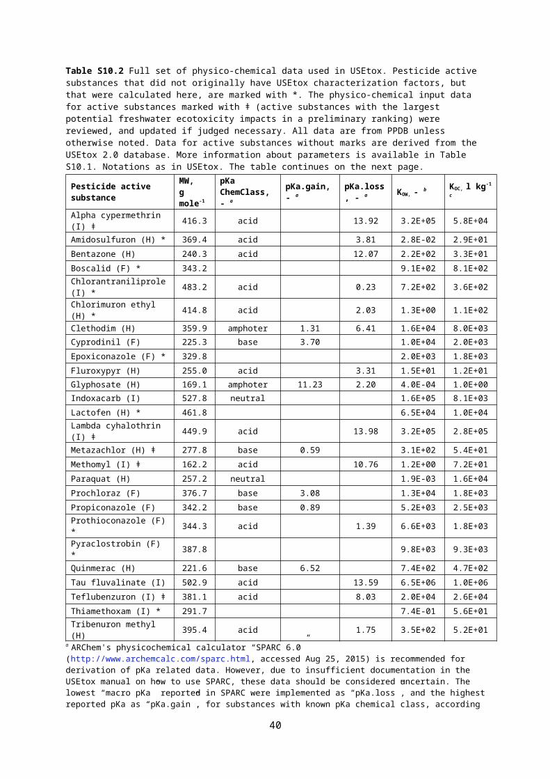
Table S10.2 Full set of physico-chemical data used in USEtox. Pesticide active substances that did not originally have USEtox characterization factors, but that were calculated here, are marked with *. The physico-chemical input data for active substances marked with ǂ (active substances with the largest potential freshwater ecotoxicity impacts in a preliminary ranking) were reviewed, and updated if judged necessary. All data are from PPDB unless otherwise noted. Data for active substances without marks are derived from the USEtox 2.0 database. More information about parameters is available in Table S10.1. Notations as in USEtox. The table continues on the next page.

Pesticide active substance MW, g mole-1

pKa ChemClass, - a pKa.gain, - a pKa.loss, - a KOW, - b KOC, l kg-1 c

Alpha cypermethrin (I) ǂ 416.3 acid 13.92 3.2E+05 5.8E+04Amidosulfuron (H) * 369.4 acid 3.81 2.8E-02 2.9E+01Bentazone (H) 240.3 acid 12.07 2.2E+02 3.3E+01Boscalid (F) * 343.2 9.1E+02 8.1E+02Chlorantraniliprole (I) * 483.2 acid 0.23 7.2E+02 3.6E+02Chlorimuron ethyl (H) * 414.8 acid 2.03 1.3E+00 1.1E+02Clethodim (H) 359.9 amphoter 1.31 6.41 1.6E+04 8.0E+03Cyprodinil (F) 225.3 base 3.70 1.0E+04 2.0E+03Epoxiconazole (F) * 329.8 2.0E+03 1.8E+03Fluroxypyr (H) 255.0 acid 3.31 1.5E+01 1.2E+01Glyphosate (H) 169.1 amphoter 11.23 2.20 4.0E-04 1.0E+00Indoxacarb (I) 527.8 neutral 1.6E+05 8.1E+03Lactofen (H) * 461.8 6.5E+04 1.0E+04Lambda cyhalothrin (I) ǂ 449.9 acid 13.98 3.2E+05 2.8E+05Metazachlor (H) ǂ 277.8 base 0.59 3.1E+02 5.4E+01Methomyl (I) ǂ 162.2 acid 10.76 1.2E+00 7.2E+01Paraquat (H) 257.2 neutral 1.9E-03 1.6E+04Prochloraz (F) 376.7 base 3.08 1.3E+04 1.8E+03Propiconazole (F) 342.2 base 0.89 5.2E+03 2.5E+03Prothioconazole (F) * 344.3 acid 1.39 6.6E+03 1.8E+03Pyraclostrobin (F) * 387.8 9.8E+03 9.3E+03Quinmerac (H) 221.6 base 6.52 7.4E+02 4.7E+02Tau fluvalinate (I) 502.9 acid 13.59 6.5E+06 1.0E+06Teflubenzuron (I) ǂ 381.1 acid 8.03 2.0E+04 2.6E+04Thiamethoxam (I) * 291.7 7.4E-01 5.6E+01Tribenuron methyl (H) 395.4 acid 1.75 3.5E+02 5.2E+01

a ARChem's physicochemical calculator “SPARC 6.0” (http://www.archemcalc.com/sparc.html, accessed Aug 25, 2015) is recommended for derivation of pKa related data. However, due to insufficient documentation in the USEtox manual on how to use SPARC, these data should be considered uncertain. The lowest “macro pKa” reported in SPARC were implemented as “pKa.loss”, and the highest reported pKa as “pKa.gain”, for substances with known pKa chemical class, according to P. Fantke (pers. comm. 2015). pKa values for ASs marked with ǂ were taken from the USEtox database (not updated). pKa chemical classes for substances marked with * were derived from PPDB (since it was not known how to derive this property from SPARC). For active substances with “no dissociation” in PPDB (boscalid, epoxiconazole, pyraclostrobin), pKa values derived from SPARC were not implemented in USEtox, since it was not known if the pKa values should be implemented as proton loss or gain (a sensitivity analysis showed that whether pKa-values were implemented as loss, gain or not implemented at all, had a very small effect on resulting characterization factors). No “macro pKa” values were available in SPARC for lactofen and thiamethoxam. Due to that pKa chemical classes and/or dissociation constants for boscalid, epoxiconazole, pyraclostrobin, lactofen and thiamethoxam could not be determined, these active substances were modeled as “neutral” substances, which is the default assumption in USEtox for substances with unknown dissociation (Fantke et al. 2015b).b Converted according to KOW = 10^log(KOW) (log KOW values are used in PestLCI, see Table S10.1). KOW of lactofen from EPISuite (experimental value).c KOC of boscalid, epoxiconazole and prothioconazole from http://www.ineris.fr/substances/fr/ (accessed Aug 20, 2015).

28

http://www.archemcalc.com/sparc.html

Table S10.2 Continued Full set of physico-chemical data used in USEtox. Pesticide active substances that did not originally have USEtox characterization factors, but that were calculated here, are marked with *. The physico-chemical input data for active substances marked with ǂ (active substances with the largest potential freshwater ecotoxicity impacts in a preliminary ranking) were reviewed, and updated if judged necessary. All data are from PPDB unless otherwise noted. Data for active substances without marks are derived from the USEtox 2.0 database. More information about parameters is available in Table S10.1. Notations as in USEtox.

Pesticide active substance

KH25C,Pa m3 mole-1

Pvap25, Pa Sol25, mg l-1 a kdegA, s-1

b kdegW, s-1

b kdegSd, s-1

b kdegSl, s-1

b

Alpha cypermethrin (I) ǂ 6.9E-02 3.4E-07 1.2E-01 1.6E-05 4.5E-08 5.0E-09 8.0E-08Amidosulfuron (H) * 5.2E-04 1.3E-05 3.1E+03 1.5E-04 2.1E-07 2.3E-08 4.8E-07Bentazone (H) 2.2E-04 4.6E-04 5.0E+02 4.7E-05 2.1E-07 2.4E-08 5.7E-07Boscalid (F) * 5.2E-08 7.2E-07 4.6E+00 6.8E-06 1.3E-07 1.4E-08 3.3E-08Chlorantraniliprole (I) * 3.2E-09 6.3E-12 8.8E-01 1.3E-05 4.5E-08 5.0E-09 1.3E-08Chlorimuron ethyl (H) * 1.7E-10 4.9E-10 1.2E+03 3.2E-05 1.3E-07 1.4E-08 2.0E-07Clethodim (H) 9.4E-05 3.5E-07 1.4E+00 1.2E-04 2.1E-07 2.4E-08 2.7E-06Cyprodinil (F) 8.5E-03 4.9E-04 1.3E+01 1.5E-04 2.1E-07 2.4E-08 1.8E-07Epoxiconazole (F) * 4.7E-04 1.0E-05 6.6E+00 6.6E-06 4.5E-08 5.0E-09 3.5E-08Fluroxypyr (H) 1.1E-08 3.8E-09 9.1E+01 2.2E-05 1.3E-07 1.5E-08 1.6E-07Glyphosate (H) 2.1E-07 2.1E-06 1.1E+04 5.9E-05 5.3E-07 5.9E-08 6.7E-07Indoxacarb (I) 4.9E-04 1.6E-08 1.7E-02 3.1E-05 4.5E-08 5.0E-09 4.0E-07Lactofen (H) * 4.6E-03 9.3E-06 5.0E-01 3.4E-06 4.5E-08 5.0E-09 2.0E-06Lambda cyhalothrin (I) ǂ 2.0E-02 2.0E-07 5.0E-03 2.4E-05 4.5E-08 5.0E-09 4.6E-08Metazachlor (H) ǂ 5.9E-05 9.3E-05 4.3E+02 4.4E-05 1.3E-07 1.4E-08 7.4E-07Methomyl (I) ǂ 2.1E-06 7.2E-04 5.8E+04 5.0E-06 5.3E-07 5.9E-08 1.2E-06Paraquat (H) 5.6E-09 1.3E-05 6.2E+05 1.6E-05 2.1E-07 2.4E-08 2.9E-09Prochloraz (F) 1.7E-03 1.5E-04 3.4E+01 5.9E-05 4.5E-08 5.0E-09 4.8E-07Propiconazole (F) 1.7E-04 5.6E-05 1.1E+02 1.7E-05 1.3E-07 1.5E-08 3.7E-08Prothioconazole (F) * 3.0E-05 4.0E-07 3.0E+02 8.5E-05 4.5E-08 5.0E-09 1.6E-05Pyraclostrobin (F) * 5.3E-06 2.6E-08 1.9E+00 1.5E-04 1.3E-07 1.4E-08 1.3E-07Quinmerac (H) 1.8E-05 1.8E-05 2.2E+02 2.7E-06 2.1E-07 2.4E-08 8.2E-07Tau fluvalinate (I) 2.7E-01 2.7E-06 5.0E-03 2.2E-05 4.5E-08 5.0E-09 2.3E-06Teflubenzuron (I) ǂ 7.0E-03 9.2E-07 1.9E-02 4.6E-06 4.5E-08 5.0E-09 8.7E-08Thiamethoxam (I) * 4.7E-10 6.6E-09 4.1E+03 1.9E-04 2.1E-07 2.3E-08 6.6E-08Tribenuron methyl (H) 1.0E-08 5.2E-08 5.0E+01 2.2E-06 1.3E-07 1.5E-08 8.0E-07

a First priority was given to experimental data on water solubility at 25 °C from EPISuite (available for chlorimuron ethyl, epoxiconazole, teflubenzuron, alpha cypermethrin, lambda cyhalothrin, metazachlor and methomyl). Second priority was given to experimental data on water solubility at 20 °C from PPDB (i.e., the same data as used in PestLCI). Estimated data on water solubility at 25 °C from EPISuite were not used, due to that experimental, and verified, data at a slightly lower temperature were considered more accurate, than estimated data at the required temperature. b The required degradation rates were derived in line with the recommended procedure (Fantke et al. 2015b), with some modification: degradation rates in soil were calculated based on half-lives measured in lab at 20°C, instead of half-lives measured in field, in order to create a consistent physico-chemical data set across PestLCI and USEtox, and because lab studied were considered more standardized and representative, than field studies. For the active substances considered here, field studies often, but not always, yield shorter half-lives than lab studies. Therefore characterization factors represent – in this sense – a conservative estimate of the toxic potency.

29

S11. Ecotoxicological effect data (USEtox)

Table S11.1 Values of the avlogEC50 parameter used in USEtox. avlogEC50-values for active substances marked with ǂ were calculated here, based on ecotoxicological effect data presented in Table S11.2. avlogEC50-values and ecotoxicological effect data for substances marked with * were taken from Nordborg et al. (2014). avlogEC50-values were calculated following the recommended procedure (Fantke et al. 2015b), described in more detail in Nordborg et al. (2014). avlogEC50-values for active substances without marks were taken from the USEtox 2.0 database.

Pesticide active substance avlogEC50, log(mg l-1)

Alpha cypermethrin (I) ǂ -2.812Amidosulfuron (H) ǂ 1.070Bentazone (H) 1.990Boscalid (F) * 0.227Chlorantraniliprole (I) * -0.291Chlorimuron ethyl (H) * 0.218Clethodim (H) 0.715Cyprodinil (F) -0.175Epoxiconazole (F) * -0.576Fluroxypyr (H) 0.965Glyphosate (H) 1.466Indoxacarb (I) -0.722Lactofen (H) * -0.373Lambda cyhalothrin (I) -4.465Metazachlor (H) 0.554Methomyl (I) -0.489Paraquat (H) -0.890Prochloraz (F) -0.950Propiconazole (F) 0.059Prothioconazole (F) * -0.214Pyraclostrobin (F) * -1.558Quinmerac (H) 1.585Tau fluvalinate (I) -2.721Teflubenzuron (I) ǂ -1.329Thiamethoxam (I) * 0.759Tribenuron methyl (H) 1.598

30

Table S11.2 Ecotoxicological effect data for three active substances. New characterization factors were calculated for amidosulfuron. Teflubenzuron and alpha cypermethrin had their ecotoxicological effect data updated, since USEtox characterization factors of these active substances were based on ecotoxicological effect data from an insufficient number of trophic levels (two), hence marked as “indicative”.

Trophic level Species Days EC(L)50, mg l-1

Source Logchronic acute

Amidosulfuron (H)

Aquatic plant Lemna gibba 7 0.0092 AGRITOX -2.04Algae Scenedemus subspicatus 3 23.5 47 PPDB/AGRITOX 1.37Algae Navicula pelliculosa 4 84.2 AGRITOX 1.93Aquatic invertebrate Daphnia magna 2 18 36 PPDB/AGRITOX 1.26Fish Oncorhynchus mykiss 4 160 320 PPDB/AGRITOX 2.20Fish Lepomis macrochirus 4 50 100 AGRITOX 1.70

Teflubenzuron (I)

Crustacean - shrimp Streptocephalus sudanicus 1 0.012 0.0236 ECOTOX -1.93Crustacean - shrimp Streptocephalus sudanicus 2 0.00030 0.00059 ECOTOX -3.53Algae Scenedesmus subspicatus 3 0.010 0.020 PPDB -2.00Aquatic invertebrate Daphnia magna 1 0.50 1.0 AGRITOX -0.30Aquatic invertebrate Daphnia magna 2 0.00022 0.00044 AGRITOX -3.66Aquatic invertebrate Daphnia magna 2 0.00140 0.0028 PPDB -2.85Fish Lepomis macrochirus 4 0.0033 0.0065 PPDB -2.49Fish Carassius carassius n.a. 250 500 AGRITOX 2.40Fish Oncorhynchus mykiss n.a. 250 500 AGRITOX 2.40

Alpha cypermethrin (I)

Algea Raphidocelis subcapitata 4 0.05000 0.10 PPDB -1.30Aquatic invertebrate Daphnia magna 2 0.00015 0.0003 AGRITOX -3.82Shrimp - crustacean Paratya australiensis 4 0.000010 0.00002 ECOTOX -5.02Aquatic invertebrate Ceriodaphnia dubia, 2 tests 8 0.00014 ECOTOX -3.84Aquatic invertebrate Ceriodaphnia dubia 2 0.00012 0.00023 ECOTOX -3.94Aquatic invertebrate Ceriodaphnia dubia 1 0.00125 0.0025 ECOTOX -2.90Fish Barbus gonionotus, 2 tests 1 0.001871 0.0037 ECOTOX -2.73Fish Barbus gonionotus, 2 tests 4 0.000566 0.0011 ECOTOX -3.25Fish Cyprinus carpio, 3 tests 4 0.001597 0.00319 ECOTOX -2.80Fish Cyprinidae, 2 tests 1 0.00249 0.00498 ECOTOX -2.60

Fish Cyprinidae, 2 tests 2 0.00184 0.00368035 ECOTOX -2.74

Fish Cyprinidae, 2 tests 3 0.00135 0.00271 ECOTOX -2.87Fish Cyprinidae, 2 tests 4 0.000946 0.00189 ECOTOX -3.02Fish Cyprinus carpio, 3 tests 1 0.012072 0.02414 ECOTOX -1.92Fish Cyprinus carpio 2 0.002100 0.0042 ECOTOX -2.68Fish Cyprinus carpio 3 0.002000 0.004 ECOTOX -2.70Fish Cyprinus carpio, 3 tests 4 0.001597 0.00319 ECOTOX -2.80Fish Oncorhynchus mykiss, 2 tests 1 0.002500 0.005 ECOTOX -2.60Fish Oncorhynchus mykiss, 2 tests 2 0.021794 0.04359 ECOTOX -1.66Fish Oncorhynchus mykiss, 2 tests 3 0.018371 0.03674 ECOTOX -1.74Fish Oncorhynchus mykiss, 3 tests 4 0.007489 0.01498 ECOTOX -2.13

31

S12. Expressing results in relation to different functional units

The initial impact assessment due to pesticide use in the primary production of the assessed food

products yielded results in the form CTUe per kg harvested crop. These results were then converted to

impact scores in CTUe per kg food product, using an LCA model of typical conversion efficiencies in

the assessed production systems. Finally, impact scores in CTUe per kg food product were converted

to impact scores in relation to different functional units (Mcal, kg protein, kg digestible protein, kg

PQI-adjusted protein in three dietary contexts).

Impact scores in CTUe/Mcal were calculated by dividing impact scores in CTUe/kg food, by energy

content/kg food (kcal/kg), and multiplying with 1000 (to convert from k to M). Data on energy

content/kg food were obtained from the Swedish Food Composition Database (see Table S12.1).

Impact scores in CTUe/kg protein were calculated by dividing impact scores in CTUe/kg food, by kg

protein/kg food. Data on kg protein/kg food were taken from Sonesson et al. (2016).

Impact scores in CTUe/kg digestible protein were calculated by dividing impact scores in CTUe/kg

food, by kg digestible protein/kg food. Data on kg digestible protein/kg food were taken from

Sonesson et al. (2016).

Impact scores in CTUe/kg PQI-adjusted protein (AD) were calculated by dividing impact scores in

CTUe/kg food, by the dimensionless PQI-values for average Swedish diet (AD). PQI-values were

taken from Sonesson et al. (2016).

32

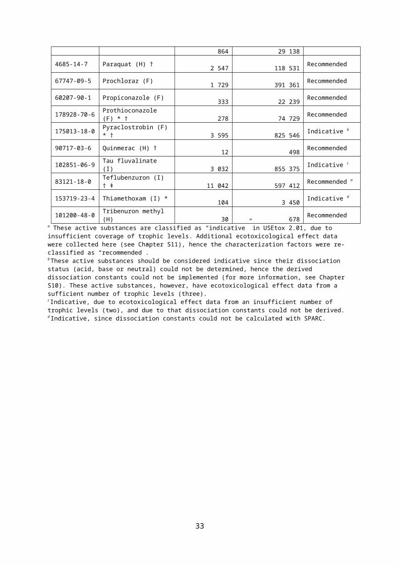
Table S12.1 Data used to convert impact scores expressed in CTUe per kg harvest crop, to impact scores in CTUe expressed in relation to the functional units Mcal, kg protein, kg digestible protein, and kg PQI-adjusted protein for an average Swedish diet (AD).

Chicken fillet

Minced pork

Minced beef Milk Pea soup Wheat bread

CTUe/kg food a 1.4E-02 1.7E-02 5.0E-03 2.9E-04 1.1E-04 2.0E-04

kg protein/kg food b 0.260 0.264 0.256 0.035 0.051 0.090

kg digestible protein/kg food b 0.247 0.250 0.243 0.033 0.040 0.084

PQI AD (-) b 21.95 24.63 20.54 4.14 3.39 7.39

kcal/kg food c 1870 2496 d 2250 473 777 2472

Food products as defined in the Swedish Food Composition Database

Kyckling bröst m skinn stekt

Gris fläskfärs fett 15% stekt

Nötfärs fett 10% stekt

Mellanmjölk fett 1,5% berik m D-vitamin

Ärtsoppa vegetarisk

Bröd vitt fibrer ca 5% typ Jättefranska

Food products as defined in the Swedish Food Composition Database (own English translations)

Chicken breast with skin pan-fried

Minced pork 15% fat pan-fried

Minced beef fat 10% pan-fried

Drinking milk fat 1,5% enriched with vitamin D

Vegetarian pea soup

Bread white ca 5% fibre type “Jättefranska”

a Calculated in this study.b Data from Sonesson et al. (2016).c Data from the Swedish Food Composition Database (www.slv.se), downloaded April, 2016. d Calculated, since pan-fried minced pork with 15% fat was not available in the Swedish Food Composition Database, assuming the same relation between fresh minced pork with 15% fat and pan-fried minced pork with 15% fat as between fresh minced beef with 10% fat, and pan-fried minced beef with 10% fat, using data from the Swedish Food Composition Database.

33

http://www.slv.se/

S13. Potential freshwater ecotoxicity impacts in crop production

RS FW BW GC PS OT BL0

1

2

3

4

CTU

e ha

-1 y

r-1

Figure S13.1 Yearly average potential freshwater ecotoxicity impacts per hectare, and the distribution between herbicides, fungicides and insecticides. Soybean is excluded due to its dominance, but is included in the small, inserted figure. RS = rapeseed, FW = feed wheat, BW = bread wheat, GC = grass/clover, PS = peas, OT = oats, BL = barley, SB = soybean.

Table S13.1 Potential freshwater ecotoxicity impacts in CTUe per ha and year and the relative contribution from each active substances used in the cultivation. The table continues on the next page.

Potential freshwater ecotoxicity impacts (CTUe ha-1 yr-1)

Relative contribution to total impact from active substances (%)

RapeseedMetazachlor 1.11 82%Quinmerac 0.06 4%Boscalid 0.10 7%Indoxacarb 0.05 3%Glyphosate 0.04 3%Total 1.36 100%Feed wheatTribenuron methyl 0.00 0%Fluroxypyr 0.08 7%Prochloraz 0.52 50%Pyraclostrobin 0.31 30%Prothioconazole 0.03 3%Tau fluvalinate 0.06 6%Glyphosate 0.04 4%Total 1.04 100%OatsTribenuron methyl 0.00 0%Lambda cyhalothrin 2.94 92%Pyraclostrobin 0.20 6%Glyphosate 0.04 1%

34

RS FW BW GC PS OT BL SB0

10

20

30

CTU

e ha

-1 y

r-1

Total 3.18 100%Table S13.1 Continued Potential freshwater ecotoxicity impacts in CTUe per ha and year and the relative contribution from each active substances used in the cultivation.

Potential freshwater ecotoxicity impacts (CTUe ha-1 yr-1)

Relative contribution to total impact from active substances (%)

Bread wheatTribenuron methyl 0.00 0%Fluroxypyr 0.08 6%Prochloraz 0.52 44%Pyraclostrobin 0.45 38%Prothioconazole 0.05 4%Tau fluvalinate 0.06 5%Glyphosate 0.04 4%Total 1.18 100%BarleyTribenuron methyl 0.00 0%Pyraclostrobin 0.24 6%Cyprodinil 0.17 4%Propiconazole 0.12 3%Lambda cyhalothrin 3.44 86%Glyphosate 0.04 1%Total 4.01 100%Grass/clover Amidosulfuron (applied year 1) 0.01 10%Glyphosate (applied year 3) 0.08 90%Total 0.08 100%PeasBentazone 0.01 2%Alpha cypermethrin 0.69 93%Glyphosate 0.04 6%Total 0.74 100%Broad beansBentazone 0.01 7%Pyraclostrobin 0.05 30%Boscalid 0.07 38%Glyphosate 0.04 24%Total 0.17 100%SoybeanParaquat 0.14 0%Lactofen 0.41 1%Alpha cypermethrin 1.56 5%Methomyl 5.49 16%Bentazone 0.03 0%Lactofen 0.40 1%Chlorimuron ethyl 0.03 0%Chlorantraniliprole 0.07 0%Clethodim 0.00 0%Pyraclostrobin 0.19 1%Chlorantraniliprole 0.07 0%Pyraclostrobin 0.14 0%Epoxiconazole 1.89 6%Chlorantraniliprole 0.13 0%Pyraclostrobin 0.14 0%Epoxiconazole 2.17 6%Teflubenzuron 0.74 2%Thiamethoxam 0.00 0%Lambda cyhalothrin 18.61 55%Paraquat 1.62 5%Total 33.82 100%

35

S14. Pesticide active substances with largest impact scores

Table S14.1 Pesticide active substances with the largest (≥ 0.1 mCTUe kg-1) potential freshwater ecotoxicity impacts, and corresponding impact scores in CTUe ha-1 yr-1. This threshold (0.1 mCTUe kg-1) is arbitrary, but useful, in identifying a handful of the active substances with largest potential impact scores. Impact scores of active substances applied more than once per crop, have been added prior to ranking. Characterization factors of active substances marked with * were calculated in this study. H = herbicide, F = fungicide, I = insecticide.

Pesticide active substances a mCTUe kg-1 CTUe ha-1 yr-1 Crop

Lambda cyhalothrin (I) 5.97 18.6 Soybean

Methomyl (I) 1.76 5.5 Soybean

Epoxiconazole (F, 2 applications) 1.30 4.1 Soybean

Lambda cyhalothrin (I) 0.73 3.4 Barley

Lambda cyhalothrin (I) 0.65 2.9 Oats

Paraquat (H, 2 applications) 0.56 1.8 Soybean

Alpha cypermethrin (I) 0.50 1.6 Soybean

Metazachlor (H) 0.33 1.1 Rapeseed

Lactofen (H, 2 applications) 0.26 0.8 Soybean

Teflubenzuron (I) 0.24 0.7 Soybean

36

S15. Potential freshwater ecotoxicity impacts of broad beans

Table S15.1 Pesticide application data for broad beans. Data from rows 112-120 in tab "scenario 2" in Excelfile "HBMV tid och bränsle för fältarbete samt pesticider HPPL" (Sonesson et al., 2014). H = herbicide. F = fungicide. I = insecticide. For broad beans, data from “scenario 2” was considered most representative of current, typical and realistic use of pesticides (the reference scenario did not include any pesticides).








Application method

Tillage type

Application month

H Basagran SG Bentazone 0.60 870 1 0.5220 522.0 Peas I Conv. boom

potato Conv. April

FSignum

Pyraclostrobin 0.50 67 0.2 0.0335 6.7 Peas III Conv. boom potato Conv. Aug.

F Boscalid 0.50 267 0.2 0.1335 26.7 Peas III Conv. boom potato Conv. Aug.

H Roundup Bio Glyphosate 3.00 360 0.25 1.0800 270.0 Bare soil Conv. boom

bare soil Conv. Sept.

Table S15.2 Key input data and results for potential freshwater ecotoxicity impacts in CTUe (Comparative Toxic Units ecotoxicity) for broad beans.

Cultivation region Crop yield (ton ha-1 yr-1)

ResultsCTUe ha-1 yr-1 CTUe kg-1 harvested crop

Plain region, Västra Götaland 3.3 0.17 5.2E-05

The favorable result of broad beans is explained by a combination of the use of active substances with relatively large emissions, but low ecotoxic potencies

(bentazone, glyphosate), and the use of active substances with relatively high ecotoxic potencies, but low emissions (pyraclostrobin, boscalid).

37

S16. Alternative soy-free feed rations for pigs and chickens: data and results

The alternative locally-sourced and soy-free, feed rations are based on the reference feed-rations in

Göransson et al., (2014) for pigs, and Wall et al., (2014) for chickens.

Table S16.1 Average soy-free feed rations for chickens and pigs.

Feed ingredientsConsumed feed (kg feed per kg food product consumed in the household)

Chicken fillet Minced porkBroad beans 0.41 1.30Wheat fodder meal 0.41Winter wheat 2.98 2.48Rapeseed 1.14 0.20Oats 1.21Barley 2.98Total 4.94 8.17

Table S16.2 Key data about the reference and alternative, soy-free, feed rations for chicken (from HBMV Scenario 3 in Wall et al., 2014).

Feed ingredients Reference feed ration (%) Soy-free feed ration (%)Wheat 62.6 36Oats 0 0Wheat meal 0 10Soy meal 25.7 0Oilseed rape meal 1.7 8Rapeseed 2.3 5Rape oil 2 0Peas 0 15Broad bean 0 10Drank 0 10Fatty acids 2 2.19CACO2 1.59 1.66Sodium chloride 0.24 0.18Mono Calcium phosphate 0.73 0.4DL- methionin 0.24 0.27L-Lysin HCL 0.37 0.52L-Treonin 0.07 0.24Premix vitamines and trace elements 0.5 0.5% dry matter 88 88Energy content, MJ/kg 12.5 12Days to slaughter, 1900 g live weight 34 37kg feed/kg live weight 1.70 1.81

38

Table S16.3 Key data about the reference and alternative, soy-free, feed rations for pigs (from HBMV Scenario 3 in Göransson et al., 2014).

Feed ingredientsReference feed ration Soy-free feed rationDry sows

Lactating sows

Piglets Pig Dry sows

Lactating sows

Piglets Pig

Wheat (10.5 %Rp) % 24.2 31.6 30.2 32.8 28.4 31.3 25.6 30.8Barley % 50 35.5 35 35 54.5 36 32.5 35Oats % 10 15.5 15 15 14.5 15 12.5 15Soymeal % 9.3 8.8 16.7 9.6 0 0 0 0Rapseedmeal % 4 6 0 5 0 0 6.2 0Faba bean % 0 0 0 0 0 15.6 20 16.3Lime % 1.29 1.36 1.38 1.2 1.73 1.67 1.38 1.53MCP % 0.56 0.55 0.63 0.45 0.1 0.36 0.52 0.17Phytase % 0.1 0.1 0.1 0.1 0.1 0.1 0.1 0.1L-lysine % 0.02 0.14 0.32 0.3 0.13 0.26 0.42 0.36L-threonine % 0.01 0 0.09 0.06 0.03 0.1 0.16 0.14DL-Methionine % 0 0 0.05 0.02 0 0.06 0.13 0.09L-Tryptophane % 0 0 0 0.02 0 0.02 0.04 0.03Vitamins % 0.5 0.5 0.05 0.05 0.5 0.5 0.5 0.5TS% 87.3 87.4 87.4 87.4 87.2 87.2 87.3 87.2MJ Net energy sows 9.44 9.4 9.21 9.2 9.4 9.55 9.2 9.4Rp g/kg 144 148 165 151 101 129 153 132P g/kg 4.8 4.9 4.9 4.7 3.1 4.2 5.2 3.7K g/kg 6.7 6.8 7.5 6.8 4.8 6.2 7.1 6.3Ca, g/MJ Net energy sows 7 7.4 7.4 6.5 7.1 7.6 7.3 6.7Sislys, g/MJ Net energy sows 0.6 0.72 1 0.86 0.4 0.72 1 0.81smbP g/MJ Net energy sows 0.27 0.34 0.35 0.32 0.22 0.29 0.35 0.25

Table S16.4 Resulting potential freshwater ecotoxicity impacts in the reference and alternative, soy-free, feed rations for chickens and pigs.

Feed ingredientsReference feed ration (CTUe / kg food) Soy-free feed ration (CTUe / kg food)Chicken fillet Minced pork Chicken fillet Minced pork

Wheat 4.73E-04 4.95E-04 5.97E-04 4.35E-04Rapeseed 9.38E-05 2.83E-04 3.28E-04 5.11E-05Soybean 1.03E-02 8.67E-03Barley 2.80E-03 2.49E-03Oats 9.45E-04 9.02E-04PeasGrass/cloverBroad beans 2.43E-05 7.64E-05Total 1.08E-02 1.32E-02 9.49E-04 3.96E-03

39

S17. Pesticide active substances with largest emissions

Table S17.1 Active substances with top-five largest emissions to air and surface water as a fraction of the applied dose, and as emitted mass. All entries are arranged in descending order (1 = highest). The crops in which the active substances are used are given in parenthesis. RS = rapeseed, FW = feed wheat, BW = bread wheat, BL = barley, OT = oats, GC = grass/clover, PS = peas, SB = soybean.

Largest emissions to air / surface water, per application

Fraction of the applied dose, % Mass emitted, kg AS ha-1

Air Surface water Air Surface water

1 Methomyl (SB)

Glyphosate (GC)

Methomyl (SB)

Glyphosate (GC)

2 Propiconazole (BL) Glyphosate (RS, FW, BW, BL, OT & PS)

Prochloraz (BW, FW)

Glyphosate (RS, FW, BW, BL, OT & PS)

3 Prochloraz (BW, FW)

Quinmerac (RS)

Bentazone (SB)

Metazachlor (RS)

4 Cyprodinil (BL) Tribenuron methyl (OT, BL) Glyphosate (GC)

Quinmerac (RS)

5 Teflubenzuron (SB) Amidosulfuron (GC) Bentazone (PS)

Bentazone (SB)

40

S18. Limitations

Only direct application of pesticides in the primary production of the crops and the associated

emissions to air and surface water, are considered. Emissions to other environmental

compartments, e.g., ground water, are not considered. Emissions to ground water could not be

taken into account, since USEtox does not provide characterization factors for emissions to

this compartment.

Emissions to agricultural soil, and impact that take place in the field, were not accounted for,

since the field is considered part of the technosphere (integrated assumption in the PestLCI

modeling framework).

Accidental spills and emissions that originate from handling and storage of pesticides are not

included, and neither are emissions that originate from other stages in the life cycle of

pesticides.

Only the active substances in herbicides, fungicides and insecticides are included. Other

ingredients in pesticide products, such as solvents and surfactants, were not included.

Pesticides used to treat seeds, inorganic substances and molluscicides, are not included.

Pesticide degradation products were not taken into account, partly due to model limitations,

and partly due to lack of data. Mixture toxicity was not accounted for, partly due to model

limitations.

Drainage systems are often installed below 1 m depth, while the soil in PestLCI is only

modelled down to a depth of 1 m. Due to this, we did not consider drainage i.e., assumed that

drainage systems were not installed. This is however not an accurate representation of

Sweden, where approximately 55% of all croplands had installed drainage systems in 2010

(Larsson et al. 2013). In Brazilian soybean cultivation on the other hand, drainage systems are

not widely used (D. Meyer, pers. comm., 2013). The fact that we did not consider drainage

systems in Sweden, may imply that emission results, and hence impact scores, are

underestimated.

Only aquatic freshwater ecotoxicity is included, while terrestrial and marine ecotoxicity, and

human toxicity, are not included (partly due to lack of impact assessment models). In

particular, ecotoxicity to pollinators is not included.

41

References

BIRKVED, M.; HAUSCHILD, M. Z. (2006) PestLCI—A model for estimating field emissions of pesticides in agricultural LCA. Ecological Modelling, 198, 433-451.

BUHL, K.; BOND, C.; STONE, D. (2013) Iron Phosphate General Fact Sheet; National Pesticide Information Center, Oregon State University Extension Services. http://npic.orst.edu/factsheets/ironphosphategen.html (accessed Aug. 5, 2015).

D. MEYER. Round Table of Responsible Soy. Personal communication, 2013.DIJKMAN, T. J., BIRKVED, M.; HAUSCHILD, M. Z. (2012) PestLCI 2.0: a second generation

model for estimating emissions of pesticides from arable land in LCA. The International Journal of Life Cycle Assessment, 17, 973-986.

FANTKE, P. (ED.), HUIJBREGTS, M., HAUSCHILD, M., JOLLIET, O., MARGNI, M., MCKONE, T.E., ROSENBAUM, R.K., VAN DE MEENT, D. (2015a) USEtox 2.0 User Manual (version 2), http://usetox.org.

FANTKE, P. (ED.), HUIJBREGTS, M., MARGNI, M., VAN DE MEENT, D. JOLLIET, O., ROSENBAUM, R.K., MCKONE, T.E., HAUSCHILD, M. (2015b) USEtox 2.0 Manual: Organic substances (version 2), http://usetox.org.

FANTKE, P. USEtox manager. Technical University of Denmark. Personal communication, 2015.GÖRANSSON, L., BARR, U. K., BORCH, E., BRUNIUS, C., FLORÉN, B., GUNNARSSON, S.,

HAMBERG, L., LINDBOM, I., LORENTZON, K., NIELSEN, T., NORMANN, A., SALOMON, E., SINDHÖJ, E., SONESSON, U., SUNDBERG, M., ÅSTRÖM, A., ÖSTERGREN, K. (2014) Hållbara matvägar – referens- och lösningsscenarier för grisproduktion och framställning av rökt skinka. SIK-report 887 (In Swedish). Gothenburg: The Swedish Institue for Food and Biotechnology (SIK).

J. KREUGER. Centre for Chemical Pesticides, Swedish University of Agricultural Sciences. Personal communication, 2015.

JANTALIA, C. P.; RESCK, D. V.; ALVES, B. J.; ZOTARELLI, L.; URQUIAGA, S.; BODDEY, R. M. (2007) Tillage effect on C stocks of a clayey Oxisol under a soybean-based crop rotation in the Brazilian Cerrado region. Soil Tillage Res. 95 (1), 97-109.

JARVIS, A., REUTER, H. I., NELSON, A., GUEVARA, E. (2008) Hole-filled seamless SRTM data V4, International Centre for Tropical Agriculture (CIAT).

KEMI (2014) Försålda kvantiteter av bekämpningsmedel, Sveriges officiella statistik 2013. Kemikalieinspektionen: Stockholm.

KEMI (2015) Bekämpningsmedelsregistret (the Pesticide database). The Swedish Chemicals Agency: Sundbyberg http://webapps.kemi.se/BkmRegistret/Kemi.Spider.Web.External/ (accessed Aug 11, 2015).

LARSSON, T., DE MARÉ, L., LINDMARK, P., RANGSJÖ, C-J., JOHANSSON, T. (2013) Jordbrukets markavvattningsanläggningar i ett nytt klimat (in Swedish). Swedish Board of Agriculture: Jönköping.

NORDBORG, M., CEDERBERG, C. & BERNDES, G. (2014) Modeling Potential Freshwater Ecotoxicity Impacts Due to Pesticide Use in Biofuel Feedstock Production: The Cases of Maize, Rapeseed, Salix, Soybean, Sugar Cane, and Wheat. Environmental Science & Technology, 48, 11379-11388.

PPDB. Pesticide Properties DataBase. Agriculture & Environment Research Unit, University of Hertfordshire; http://sitem.herts.ac.uk/aeru/footprint/index2.htm (accessed Sept 2, 2015)

42

http://webapps.kemi.se/BkmRegistret/Kemi.Spider.Web.External/

http://usetox.org/

ROSENBAUM, R. K.; BACHMANN, T. M.; GOLD, L. S.; HUIJBREGTS, M. A. J.; JOLLIET, O.; JURASKE, R.; KOEHLER, A.; LARSEN, H. F.; MACLEOD, M.; MARGNI, M.; MCKONE, T. E.; PAYET, J.; SCHUMACHER, M.; VAN DE MEENT, D.; HAUSCHILD, M. Z. (2008) USEtox – the UNEP-SETAC toxicity model: recommended characterization factors for human toxicity and freshwater ecotoxicity in life cycle impact assessment. Int. J. Life Cycle Assess. 13 (7), 532-546.

SJV (2015a) Bekämpningsrekommendationer, svampar och insekter 2015. Jönköping: Jordbruksverket.

SJV (2015b) Kemisk ogräsbekämpning, våren 2015. Jönköping: Jordbruksverket.SLU (2015) Paths to a sustainable food sector (Hållbara Matvägar). Project homepage. [Online].

Swedish University of Agricultural Sciences. Available: http://www.slu.se/sv/centrumbildningar-och-projekt/hallbara-matvagar/.

SONESSON, U., LORENTZON, K., FLORÉN, B., KREWER, C., KUMM, K. I., NILSSON, K. & WOODHOUSE, A. (2014) Hållbara matvägar – resultat och analys [Paths to a sustainable food sector: Results and analysis]. SIK-rapport 891 (In Swedish). Gothenburg: The Swedish Institue for Food and Biotechnology (SIK).

SONESSON, U., DAVIS, J., FLYSJÖ, A., GUSTAVSSON, J., WITTHÖFT, C. (2016) Protein quality as functional unit—A methodological framework for inclusion in life cycle assessment of food. Submitted for publication.

STENBERG, B., SONESSON, U., STENBERG, M. & LORENTZON, K. (2014) Hållbara matvägar – utgångs- och lösningsscenarier för växtodling. SIK-report 890 (In Swedish). Gothenburg: The Swedish Institue for Food and Biotechnology (SIK).

SWEDISH AGRICULTURAL SOIL INVENTORY DATABASE. Department of soil and environment, Swedish Univeristy of Agricultural Sciences. http://www-jordbruksmark.slu.se/ (accessed 2 Sept, 2015).

WALL, H., BARR, U. K., BORCH, E., BRUNIUS, C., GUNNARSSON, S., HAMBERG, L., LINDBOM, I., LORENTZON, K., NIELSEN, T., NILSSON, K., NORMANN, A., SALOMON, E., SINDHÖJ, E., SONESSON, I., SUNDBERG, M., ÅSTRÖM, A., ÖSTERGREN, K. (2014) Hållbara matvägar – referens- och lösningsscenarier för kycklingproduktion och framställning av fryst kycklingfilé. SIK-report 888 (In Swedish). Gothenburg: The Swedish Institue for Food and Biotechnology (SIK).

43

http://www.slu.se/sv/centrumbildningar-och-projekt/hallbara-matvagar/

study regions - ars.els-cdn.com · web viewthe plain region is defined as the municipalities...

Documents