study on the rheology of drilling fluid and its impact on
TRANSCRIPT

WA School of Mines: Minerals, Energy and Chemical Engineering
Study on the Rheology of Drilling Fluid and Its Impact on Drilling
Operation
Yiwen Wang
This thesis is presented for the Degree of
Master of Philosophy (Petroleum Engineering)
of
Curtin University
October 2019

1
Declaration
To the best of my knowledge and belief this thesis contains no material previously published
by any other person except where due acknowledgement has been made.
This thesis contains no material which has been accepted for the award of any other degree
or diploma in any university.
Signature: Yiwen Wang
Date: 20 October, 2019

2
Acknowledgements I would first like to express my deepest gratitude to my thesis advisor and research supervisor,
Dr Masood Mostofi, who provides me infinite encouragement and inspiration throughout my
study and life. I appreciate his persistent guidance and help me to embark the research journey.
His personality and passion for work will influence and motivate me to make constant progress
in my future work.
Having this opportunity, I would like to thank Dr Dimple Quyn for her valuable advice and
discussions throughout the process of thesis writing, which had a great influence on this
graduation thesis.
I would like to acknowledge the Australian Federal Government for the financial support of
Australian Postgraduate Awards (APA) during the whole period of my study at Curtin
University.
I am grateful to everyone in our Drilling Mechanics Group. The completion of this thesis work
was impossible without the support of all of them. I am glad to be among of this research team.
Finally, special thanks to my lovely parents, Jianlin Wang and Yan Zhang, for their endless
love and support during my life.

3
Contents
Abstract .................................................................................................................................... 9
Chapter 1. Introduction .......................................................................................................... 10
1.1. Background ................................................................................................................. 10
1.2. Objective ..................................................................................................................... 12
1.3. Significance ................................................................................................................. 13
Chapter 2. Literature review .................................................................................................. 14
2.1. Drilling fluid rheology ................................................................................................ 14
2.2. Rheological models ..................................................................................................... 16
2.3. Rheological measurement methods ............................................................................ 18
2.3.1. Marsh Funnel measurement ................................................................................. 18
2.3.2. Rotary viscometer measurement .......................................................................... 18
2.3.3. Pipe viscometer measurement .............................................................................. 21
2.4. Rheology measurement conditions ............................................................................. 25
2.5. Influence of particles on drilling fluid rheology ......................................................... 25
2.5.1. Solid particles in drilling fluid ............................................................................. 26
2.5.2. Suspensions in drilling fluid ................................................................................ 27
2.5.3. Effect of solid particles on fluid rheology ............................................................ 28
2.5.4. Viscosity models of suspensions .......................................................................... 31
2.6. Polymer synergy ......................................................................................................... 33
Chapter 3. Methodology ........................................................................................................ 36
3.1. Introduction ................................................................................................................. 36
3.2. Rheological measurement ........................................................................................... 36
3.2.1. Ofite measurement ............................................................................................... 36
3.2.2. Haake measurement ............................................................................................. 37
3.2.3. Capillary measurement ........................................................................................ 39
3.3. Test material ................................................................................................................ 45
3.3.1. Additives .............................................................................................................. 45
3.3.2. Solid particles ....................................................................................................... 47
Chapter 4. Results and Discussion ......................................................................................... 49
4.1. Benchmarking of different rheology measurement techniques ................................... 49
4.2. Synergetic interaction ................................................................................................. 64
4.3. Particle effect on rheology .......................................................................................... 68
Chapter 5. Conclusion ............................................................................................................ 81
5.1. Effective methods of drilling fluid viscosity measurement ........................................ 81
4
5.2. CtrolTM and CTrolXTM drilling fluids .......................................................................... 82
5.3. Effect of fine particles on mono-dispersed suspension rheology ................................ 82
5.4. Recommendations for future work ............................................................................. 84
References .............................................................................................................................. 85
Appendices ............................................................................................................................. 88
Appendix A - AMC GUAR GUM ..................................................................................... 88
Appendix B - AMC PAC-R ............................................................................................... 89
Appendix C - AMC GEL XTRA ....................................................................................... 90
Appendix D - COREWELL ............................................................................................... 91
Appendix E – AMC XAN BORE ...................................................................................... 92
5
List of Figures
Figure 1: Schematic of the drilling fluid circulation system. ................................................. 11 Figure 2: Newtonian fluid, shear thinning and shear thickening of Non-Newtonian fluids: (a) variation of shear stress with shear rate, (b) variation of viscosity with shear rate. .............. 15 Figure 3: Thixotropic behaviour of Non-Newtonian fluids: the variation of shear stress and shear rate with time. ............................................................................................................... 16 Figure 4: Demonstration of zero shear and infinite shear viscosity for a polymer. ............... 17 Figure 5: Marsh Funnel viscosity measurement. ................................................................... 18 Figure 6: API rotary viscometer Ofite 900. ........................................................................... 19 Figure 7: Examples of other rotary viscometers: (a) Brookfield viscometer, (b) Haake Mars viscometer. ............................................................................................................................. 20 Figure 8: Different spindle sets of Brookfield viscometer. ................................................... 20 Figure 9: Different sensor geometries of Haake Mars: (a) Cone-Plate, (b) Plate-Plate and (c) Cylinder. ................................................................................................................................ 21 Figure 10: Pipeline viscometer system. ................................................................................. 22 Figure 11: Wall shear stress versus nominal wall shear rate. ................................................ 24 Figure 12: Effect of temperature and pressure on rheology of a certain fluid. ...................... 25 Figure 13: Monodisperse and poly-disperse suspensions with particles. .............................. 27 Figure 14: Properties of drilling fluids with different volume concentration of cuttings within same size. .............................................................................................................................. 27 Figure 15: The impact of increasing particles concentration on the apparent viscosity of suspension. ............................................................................................................................. 29 Figure 16: The impact of particles size on the apparent viscosity of silica sand based suspension. ............................................................................................................................. 29 Figure 17: The increase of suspension apparent viscosity by increasing particles size. ........ 30 Figure 18: The conceptual picture of agglomerated particles and chain structure particles. . 30 Figure 19: The conceptual picture of flow behaviour of suspensions at different shear rate. 31 Figure 20: Drilling cuttings agglomeration in high angle well borehole section. .................. 33 Figure 21: Viscosity synergism between Xanthan Gum and Guar Gum. .............................. 35 Figure 22: Ofite 900 viscometer with R1B1 geometry. ........................................................ 36 Figure 23: Haake RheoWin 3 interface-real time graph. ....................................................... 37 Figure 24: MATLAB analysis of Haake step-wise measurement of one suspension with particles. ................................................................................................................................. 38 Figure 25: Example of the variation of shear rate with time during a thixotropic loop test of suspension. ............................................................................................................................. 38 Figure 26: Hysteresis loop test of suspension sample – Haake RheoWin 3 real time graph. 39 Figure 27: Straight pipe viscometer. ..................................................................................... 40 Figure 28: SIEMENS flow transmitter FM Mag 5000 and SITRANS F M TRANSMAG 2. 40 Figure 29:MRB20 absolute pressure transmitter and Keller differential pressure sensor. ... 41 Figure 30: Pressure sensor calibration setup made of 6 meters vertical pipe. ...................... 41 Figure 31: DAQ SomatXR MX840B-R data acquisition system. ......................................... 42 Figure 32: CatmanEasy Interface– real time graph. ............................................................... 42 Figure 33: The variation of bias measurement of absolute and differential pressure sensors during an experiment. The bias was measured multiple times during the experiment. ......... 43 Figure 34: Pressure drop equation of Bingham plastic model fluid. . .................................... 44 Figure 35: Pressure drop equation of Power law model fluid. .............................................. 44 Figure 36: Pressure drop equation of H-B model fluid. ........................................................ 44 Figure 37: AMC Xanthan Gum (XanboreTM) of suspending fluid. ....................................... 46
6
Figure 38 : The storage tank with the agitator. ...................................................................... 46 Figure 39: Sieve shaker (left) and sieve meshes (right) for 200 μm, 150 μm, 106 μm, and 75 μm (top to bottom). ............................................................................................................... 47 Figure 40: Comparison of fluid viscosity of a polymer and a bentonite solution using Ofite 900 R1B1 rotary viscometer. ................................................................................................ 49 Figure 41: Haake Mars Z20DIN, PP35Ti and C35/4Ti sensor systems. .................................. 50 Figure 42: Rheological measurement of 0.3 wt. % Xanthan Gum measuring with different geometries of Haake Mars. .................................................................................................... 51 Figure 43: Comparison of rheological measurements with Haake Z20DIN, Ofite R1B1 and R1B2 geometries. ................................................................................................................... 52 Figure 44: MATLAB interface of pressure drop experiment of 0.5 inch straight pipe viscometer. ............................................................................................................................. 52 Figure 45: Wall shear stress versus nominal shear rate. ........................................................ 55 Figure 46: The logarithmic plot of wall shear stress versus nominal shear rate. ................... 56 Figure 47: Comparison of 6 wt. % bentonite rheological measurements with 0.5 inch straight pipe viscometer and Ofite 900 viscometer. ............................................................................ 57 Figure 48: Comparison of 6 wt. % bentonite rheological measurement with 0.75 inch pipe viscometer (using differential sensor Keller) and Ofite viscometer. ..................................... 58 Figure 49: Comparison of 6 wt. % bentonite rheological measurement with 0.75 inch pipe viscometer (using absolute sensors MRB20) and Ofite viscometer. ..................................... 59 Figure 50: Comparison of 6 wt. % bentonite rheological measurement with 0.5 inch, 0.75 inch pipe viscometer and Ofite 900 viscometer. ................................................................... 60 Figure 51: Comparison of 6 wt. % bentonite rheological measurement with 1 inch pipe viscometer and Ofite 900 viscometer. .................................................................................... 61 Figure 52: Full rheological measurement of 6 wt. % bentonite using Ofite 900 viscometer. 62 Figure 53: Pressure loss predictions of three different rheological models. .......................... 63 Figure 54: Rheological measurement of viscosifiers from 0 1/s to 1900 1/s. ....................... 64 Figure 55: Results of changing weight concentrations of additives for development of CTrolXTM. ............................................................................................................................. 65 Figure 56: Repeatability of CtrolTM measurements. ............................................................... 66 Figure 57: Coiled tube drilling system, RoXplorer, used in the drilling trials in Australia - courtesy DET CRC. .............................................................................................................. 66 Figure 58: The benchmark of CtrolTM and CTrolXTM in the field (Mostofi and Samani 2017). ............................................................................................................................................... 67 Figure 59: Establishing return after CtrolTM invasion into unconsolidated formations. The data collected from the RoXplorer field trial in Victoria. (Mostofi and Samani 2018). ........ 67 Figure 60: Haake step-wise measurement of suspension with 0.3 vol. % sand at size range of 250-300 micron. ..................................................................................................................... 68 Figure 61: Comparison of viscosity of suspension with 38-75 micron CaCO3 at different volume concentration. ............................................................................................................ 69 Figure 62: Comparison of viscosity of suspension with 106-200 micron silica sand at different volume concentration. ............................................................................................ 69 Figure 63: Comparison of viscosity of suspension with 200-250 micron silica sand at different volume concentration. ............................................................................................ 70 Figure 64: Comparison of viscosity of suspension with 250-300 micron silica sand at different volume concentration. ............................................................................................ 70 Figure 65: Relative viscosity of suspensions with 3.0 vol. % particles at shear rate from 0 to 1900 1/s. ................................................................................................................................. 71

7
Figure 66: Relative viscosity of suspensions with 0.3 vol. % particles at shear rate from 0 to 2000 1/s. ................................................................................................................................. 73 Figure 67: Relative viscosity of suspensions with 1.5 vol. % particles at shear rate from 0 to 2000 1/s. ................................................................................................................................. 73 Figure 68: Thixotropic loop test of suspension with 2.4 vol. % 250-300 micron silica sand. 74 Figure 69: Thixotropic loop of suspension with 2.4 vol. % 106-200 micron silica sand. ..... 74 Figure 70: Relative viscosity of CaCO3 suspensions with different volume concentration at shear rate from 0 to 1 1/s. ....................................................................................................... 76 Figure 71: Relative viscosity of CaCO3 suspensions with different volume concentration at shear rate from 100 to 1900 1/s. ............................................................................................. 76 Figure 72: Relative viscosity of 200-250 micron sand suspensions with different volume concentration at shear rate from 0 to 1 1/s. ........................................................................... 77 Figure 73: Relative viscosity of 200-250 micron sand suspensions with different volume concentration at shear rate from 100 to 1900 1/s. .................................................................. 77 Figure 74: Relative viscosity of 38-75 micron CaCO3 with different volume concentration at specific shear rate. .................................................................................................................. 78 Figure 75: Thixotropic loop of suspension with 0.9 vol. % 106-200 micron silica sand....... 78 Figure 76: Thixotropic loop of suspension with 1.5 vol. % 106-200 micron silica sand....... 79 Figure 77: (a) variation of relative viscosity with particle concentration, (b) variation of relative viscosity with shear rate. .......................................................................................... 83 Figure 78: Variation of thixotropic loop area with particle concentration. ........................... 83
8
List of Tables
Table 1: Drilling parameters of vertical well. ........................................................................ 11 Table 2: Typical rheological models. ..................................................................................... 16 Table 3: The diameter of different Ofite 900 rotor-bob arrangement. ................................... 19 Table 4: Predicted straight pipe friction loss of a certain fluid with different rheological models. ................................................................................................................................... 24 Table 5: Structure and property relationship of Xanthan Gum. ............................................ 35 Table 6: Specification of pipe viscometers. .......................................................................... 40 Table 7: Size range of solid particles. .................................................................................... 48 Table 8: Specification of Haake Mars sensor systems. ......................................................... 50 Table 9: 0.5 inch straight pipe viscometer data for 6 wt. % bentonite. .................................. 53 Table 10: Rheological parameters of 6 wt. % bentonite measured with 0.5 inch straight pipe viscometer. ............................................................................................................................. 54 Table 11: Calculated rheological parameters of 6 wt. % bentonite measured with 0.5 inch straight pipe viscometer. ....................................................................................................... 56 Table 12: Calculated rheological parameters of 6 wt. % bentonite measured with 0.75 inch straight pipe viscometer (using differential sensor Keller). .................................................. 57 Table 13: Calculated rheological parameters of 6 wt. % bentonite measured with 0.75 inch straight pipe viscometer (using absolute sensors MRB20). .................................................. 58 Table 14: Calculated rheological parameters of 6 wt. % bentonite measured with 0.75 inch straight pipe viscometer (using average pressure drop measured by absolute and differential sensors). ................................................................................................................................. 59 Table 15: Rheological constants of 6 wt. % bentonite for 0.5 inch pipe viscometer. ............ 62 Table 16: Calculation of pressure drop of 6 wt. % bentonite in laminar flow condition measuring with 0.5 inch pipe viscometer. .............................................................................. 62 Table 17: Thixotropic loop tests of 2.4 vol. % of CaCO3 and silica sand suspensions with different particles sizes. ......................................................................................................... 75 Table 18: Thixotropic loop tests of suspensions with silica sand particle of different volume concentrations. ....................................................................................................................... 79
9
Abstract Optimisation and automation are becoming an integral part of drilling workflow in which,
drilling operation is predicted under different scenarios. In these predictions, fluid rheology is
an important component. Indeed the accuracy and effectiveness of drilling prediction and
optimisation can be significantly improved by including more realistic characteristics of fluid
rheology. The measurement and characterisation of fluid rheology in the open literature and
in the field are simplifications.
An objective of this thesis was to study the fluid rheology in more depth using different fluid
rheology methods including rotational, extensional and hydraulic viscometers. Amongst these
measurements, the Marsh Funnel viscosity test can indicate changes in fluid properties, with
basic measurements taken at atmospheric condition. The Ofite 900 and Brookfield viscometers
have advantages in measuring fluid rheology but have limitations in measuring suspensions
with cuttings. The Haake Mars viscometer, with a concentric cylinder sensor system, provides
rheological measurement over a wide range of shear rates under thermal and pressure
controlled experimental conditions, but it cannot measure suspension with particles of high
volume concentration and large size. The straight pipe viscometer can be used for flowing
fluid rheology measurement in the presence of solid particles.
In the second part of the thesis, a series of experiments was conducted to ascertain the synergic
interaction of low-end viscosifiers to enhance drilling fluid properties. In addition to laboratory
studies, a series of field applications was undertaken using RoXplorer drilling rig to compare
the efficiency of CtrolTM and CTrolXTM with two commercial drilling fluid systems.
Furthermore, rheological experiments were performed to investigate the effect of fine particles
on the rheology of mono-dispersed suspensions. It was found that a key factor affecting
viscosity of mono-dispersed suspension is the volume fraction of particles in suspension. The
particle size effect is minimum at medium and high shear rate regions.

10
Chapter 1. Introduction
1.1. Background
Drilling fluid can be considered the lifeblood of drilling operation as it provides several
different functions in the drilling industry, such as cutting evacuation from the drill bit face
and well, cutting suspension and transportation, controlling formation fluid flowing into the
borehole, stabilising and cleaning the borehole, and sealing permeable formations [1].
Therefore, the properties of drilling fluids, such as fluid density [2], viscosity [3] and the ability
to control fluid loss and filtration [4], are critical parameters that require optimisation. The
density of mud is vital for well control [5], and chemical composition significantly influences
borehole stability [6]. Mud rheology has a considerable impact on suspending and carrying
drilling cuttings, optimizing wellbore hydrodynamic pressure, and efficient cleaning of
borehole.
In drilling operation, the drilling fluid is exposed to a wide range of shear rates during one
cycle of circulation, from the low-end shear rate when pumping is stopped, to the high–end
shear rate when drilling [1]. The range of shear rates also depends on area open to flow: the
high-end and low-end shear rates may be experienced in different sections of the drilling
string/wellbore. The shear rate of drilling fluid in laminar flow cannot be measured directly
but can be calculated through the Mooney-Rabinowitsch equation [7].
where γ̇ is shear rate, U is the average velocity of the fluid and D is the diameter of the fluid
flowing area. The quantity (8U/D) or the equivalent form in this equation, also known as the
flow characteristics, provides a basic estimation of the shear rate of drilling fluid during mud
circulation. In this project, a case of vertical well drilling is experimentally simulated to
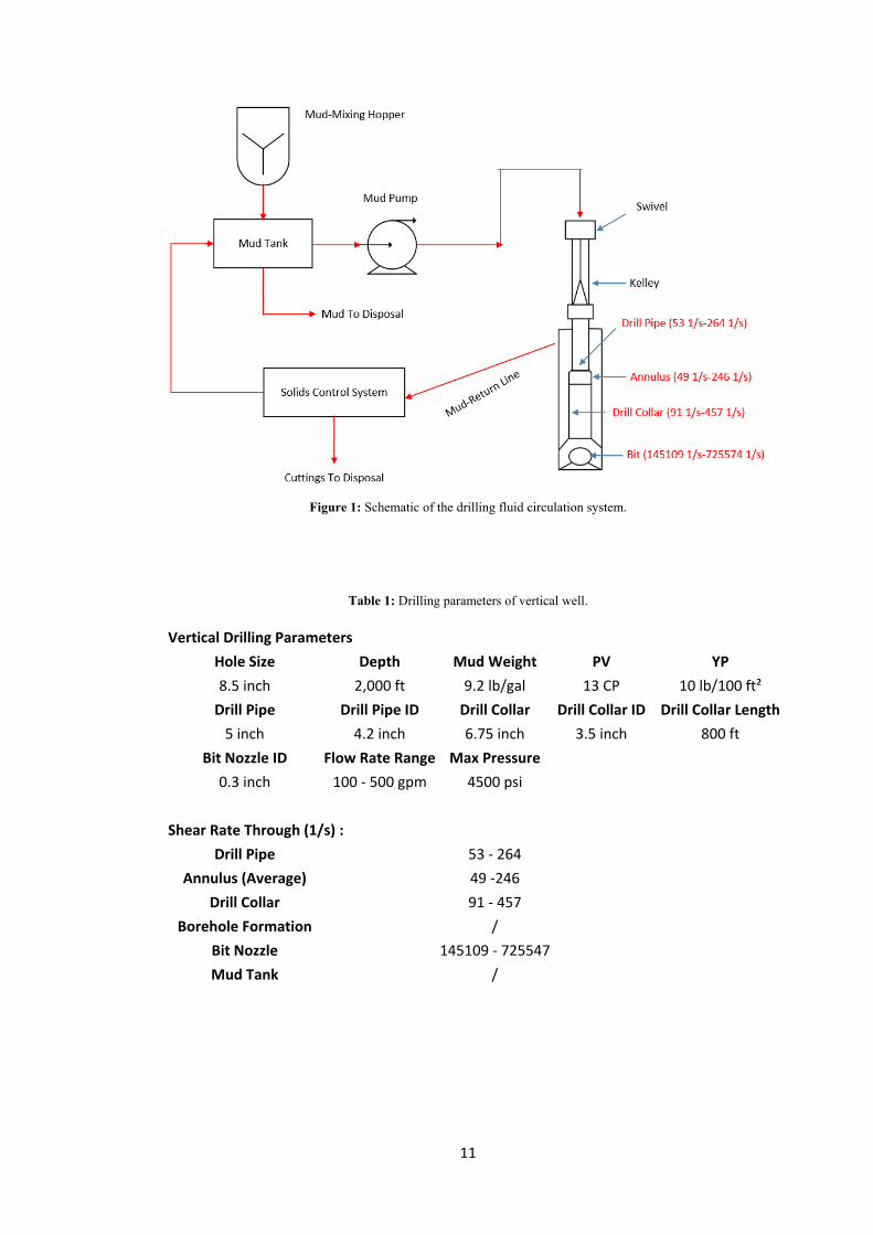
demonstrate the wide range of shear rates for mud circulation, [Figure 1] with key vertical well
drilling information is listed in Table 1. From Table 1, the calculated shear rate ranges from
0.1 1/s while the fluids are being lost into borehole formations along the fracture planes, to
approximately 103 1/s when the drilling fluid injecting out of bit nozzle, or being at the bit/rock
interface. It is important to measure and monitor the fluid rheology along all these shear rate
ranges, in order to effectively design the drilling fluid.
γ ̇ =8UD (1.1)
11
Figure 1: Schematic of the drilling fluid circulation system.
Table 1: Drilling parameters of vertical well.
Vertical Drilling Parameters Hole Size Depth Mud Weight PV YP 8.5 inch 2,000 ft 9.2 lb/gal 13 CP 10 lb/100 ft²
Drill Pipe Drill Pipe ID Drill Collar Drill Collar ID Drill Collar Length 5 inch 4.2 inch 6.75 inch 3.5 inch 800 ft
Bit Nozzle ID Flow Rate Range Max Pressure 0.3 inch 100 - 500 gpm 4500 psi
Shear Rate Through (1/s) :
Drill Pipe 53 - 264 Annulus (Average) 49 -246
Drill Collar 91 - 457 Borehole Formation /
Bit Nozzle 145109 - 725547 Mud Tank /

12
However, the oil and gas industry standard implements relatively simplified characterization
of rheology. Currently, the laboratory 10-speed viscometer (600, 300, 200, 100, 60, 30, 6, 3,
2 and 1 rpm) is used to measure the rheology of drilling mud. The rheological readings of this
viscometer at 600 rpm and 300 rpm are then applied to calculate mud plastic viscosity and
yield point, and used to describe the flow behaviour of drilling fluid. The drilling fluids are
assumed to behave with similar flow characteristic when their ϴ300 and ϴ600 values similar.
Furthermore the classical rotary viscometer Ofite or Fanne used in the drilling field cannot
measure mud rheology at very low shear rates which are below 0.1 1/s; therefore, low-shear-
rate measurement is ignored but it is very crucial for operation. Due to this deficiency in
rheology measurement for drilling operations, this research will aim to fill the gaps in drilling
fluid characterization across a wide shear rate range.
1.2. Objective
This thesis aims to obtain a better understanding of the rheology of polymer drilling fluid
solutions over an extensive range of shear rates that exceeds the range typically measured in
the drilling fluid industry. The experiments are performed with and without cuttings, to explore
the solid impact on fluid rheology. The experimental study of fluid rheology will be obtained
from three different rheology measurement techniques using the Ofite 900, the Haake Mars
and a straight pipe viscometer. These advanced and detailed measurements of fluid viscosity
will be used in conjunction with engineering models developed for specific drilling processes,
and the accurate measurement of fluid rheology using current models in characterising the
drilling processes will be investigated. Examples of these processes are fluid flowing in
straight pipes, solid suspension and solid removal.
The specific objectives of this thesis are as follows:
1) To quantify the impact of different fluid viscosifiers on the fluid rheology, and in particular
investigate how viscosity will be affected at a wide range of shear rates. Synergistic
experiments with different polymers will be investigated to pave the way for the development
of the preventative drilling fluid CtrolTM and the remedial drilling fluid CTrolXTM for particular
drilling application.
2) To investigate and study the cuttings size and concentration effects on the drilling fluid
viscosity. Different sizes of cuttings were prepared for the experiment, ranging from 1 wt. %
to 10 wt. %, which can simulate actual well downhole conditions.
3) To predict the fluid friction loss under various conditions such as fluid rheology, flow rate.
The investigations will be carried out using straight pipe viscometer with 0.5 inch diameter.
13
1.3. Significance
This research attempts to better characterise fluid rheology at a wide range of shear rates, i.e.
the fluid behaviour when the fluid is under low shear rate in the range of 0.01-0.1 1/s (e.g. in
the case of fluid loss) or high shear rates in the range of 2,000-6,000 1/s (e.g. in the case of
fluid processing in a centrifuge or hydrocyclone). In particular, this research investigates the
low-end rheology of different polymer combinations and facilitates the development of two
drilling fluid systems CtrolTM and CTrolXTM for fluid loss control. This research presents a
novel approach to determine fluid rheological parameters in real-time by using pipe viscometer,
with elimination of the efforts to apply traditional rheology measurement.
1.4. Organization of thesis
This thesis comprises a total of five chapters. Chapter 1 introduces the background of current
research and an overview of proposed topic. The research objective, the significance of this
work as well as thesis structure are presented.
In Chapter 2, the literature review of drilling fluid rheology and its impact on drilling operation
are presented. The vital role of mud rheology in drilling industry is highlighted in this chapter,
illustrating a comprehensive summary of rheology which includes flow behaviour models,
viscosity measurement techniques, cutting effect, low-end rheology, drilling fluid synergy and
fluid hydraulics.
Chapter 3 describes experimental setup for cutting effect tests and straight pipe viscometer
measurement. Detailed specification of measurement apparatus and procedures are presented.
The method of preparing the test fluid and solid particles is elaborated.
In Chapter 4, the benchmark experiments with Marsh Funnel, rotational, extensional and
capillary viscometers are provided. Different viscosity modified additives including bentonite,
natural and synthetic polymers are compared to study the interaction of additives in modifying
the low-end rheology of fluid. Experiments are performed to investigate cutting effect on the
full range rheology of polymer.
And finally, the summary of findings of this research is presented in Chapter 5 followed by
recommendation for future research in this area.
14
Chapter 2. Literature review In this chapter, a summary of previous work in the area of fluid rheology from different
engineering disciplines are reviewed. The chapter covers fluid rheological models and
different viscosity measurement techniques, and reviews previous work related to the
influence of particle cuttings on fluid rheology. In terms of fluid rheology measurement
techniques, both API and capillary viscometer techniques are discussed in details. A summary
of previous experimental studied on the synergy of polymers are also discussed at the end of
this chapter.
2.1. Drilling fluid rheology
Drilling fluid rheology plays an important role in cutting transportation and drilling hydraulics.
Due to the significance of fluid rheology in drilling operation, it has been the focus of extensive
research in petroleum engineering. However, there is considerable and relevant research into
fluid rheology in other disciplines such as such as food processing, chemical engineering and
mechanical engineering. “Rheology” is an area of science concerned with deformation and
flow of materials, which embraces viscosity, elasticity and plasticity. The term was first
invented by Eugene C. Bingham at Lafayette College in 1920 [7]. Although the study of fluid
rheology covers an immense range of engineering applications, it is especially vital for
optimization of drilling fluids and cementing slurries in terms of both fluid hydraulics and
flow behaviour of solid suspended in fluids.
Fluids can be classified to Newtonian and Non-Newtonian fluids, based on the relationship
between shear stress and shear rate,
τ = µ × γ̇
(2.1)
where τ is shear stress, µ is viscosity and γ̇ is shear rate [7]. In SI units, shear stress is in Pa,
shear rate in 1/s and viscosity in Pa.s.
Newton’s Law of Viscosity describes the simplest fluid flow behaviour: fluid viscosity is
measured as the ratio between shear stress and shear rate under constant pressure and
temperature [7]. Newtonian fluids start to flow when an infinitely small amount of shear stress
is initiated, and the shear stress increases linearly with shear rate. Many common liquids, such
as water, oil, air, gasoline and glycerine behave like a Newtonian fluid. However, fluid
characterization is far more complex and this relationship can be influenced by the timeframe
at which the shear rate is applied. No real fluids fit this mathematical description perfectly.

15
For non-Newtonian fluids, there is no constant of proportionality between shear rate and shear
stress, i.e., the viscosity varies with shear rate and time. In the case of variation of viscosity
with shear rate, fluids are classified as shear-thinning and shear-thickening fluids, [Figure 2]
[7]. The term “shear- thinning” refers to fluids exhibiting lower viscosities at higher shear rates.
The shear-thinning property is very desirable in drilling, when lower viscosity (at higher shear
rate) reduces circulating pressure, while higher viscosity is essential when circulation is
stopped to suspend drill cuttings in the well annulus, or to control the fluids loss into
permeable/fractured formations.
In contrast, there are fluids which have higher viscosities with increasing of shear rate, which
are called “shear-thickening” fluids. Examples of these fluids are corn starch-water mixtures
or suspensions with a high concentration of solid particles. These fluids do not have a
particular application in drilling operation.
Figure 2: Newtonian fluid, shear thinning and shear thickening of Non-Newtonian fluids: (a) variation of shear stress with shear rate, (b) variation of viscosity with shear rate [7].
Most drilling muds are shear-thinning thixotropic fluids; “thixotropy” means that the fluids
take time to establish equilibrium for the applied shear rate [Figure 3] [8]. This time-dependent
fluid characteristic can be quantified with a thixotropic loop test. As will be explained later,
loop tests can be performed to quantify the extent of thixotropic behaviour.

16
Figure 3: Thixotropic behaviour of Non-Newtonian fluids: the variation of shear stress and shear rate with time
[7].
2.2. Rheological models
Rheological models are mathematical correlations of shear stress with shear rate. Typical
rheological models used in the drilling industry to simulate and characterise fluid dynamics
are listed in Table 2. Not all fluids conform precisely to a single model over the entire range
of shear rates but a combination of models may be applied.
Table 2: Typical rheological models [7].
Drilling Model Equations K: Consistency index n: Power index τp: Yield point η: Apparent viscosity η0: η at γ̇ ➡ 0 η∞: η at γ̇ ➡ ∞ ơ: Relaxation time
Bingham Model τ = τp + µP × γ̇ Power Law Model τ = kγ̇n
Herschel-Bulkley Model τ = τp + kγ̇n
Cross Model η− η∞η0− η∞
= 1 + ơ x γ̇2
Carreu Model η− η∞η0− η∞
= 1 + ơ x γ̇n Casson Model √τ = �τp + �η∞γ̇
The variation of fluid viscosity with shear rate for polymers can be characterised by three
stages [9]. In the first stage, polymers behave like Newtonian fluids at very low shear rates.
The fluids exhibit shear-thinning property at medium shear rates in the second stage and at
higher shear rates, stage three shows that polymers have constant infinite shear viscosity,
[Figure 4].
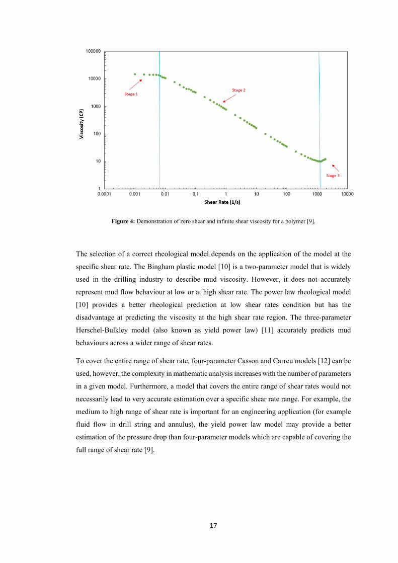
17
Figure 4: Demonstration of zero shear and infinite shear viscosity for a polymer [9].
The selection of a correct rheological model depends on the application of the model at the
specific shear rate. The Bingham plastic model [10] is a two-parameter model that is widely
used in the drilling industry to describe mud viscosity. However, it does not accurately
represent mud flow behaviour at low or at high shear rate. The power law rheological model
[10] provides a better rheological prediction at low shear rates condition but has the
disadvantage at predicting the viscosity at the high shear rate region. The three-parameter
Herschel-Bulkley model (also known as yield power law) [11] accurately predicts mud
behaviours across a wider range of shear rates.
To cover the entire range of shear rate, four-parameter Casson and Carreu models [12] can be
used, however, the complexity in mathematic analysis increases with the number of parameters
in a given model. Furthermore, a model that covers the entire range of shear rates would not
necessarily lead to very accurate estimation over a specific shear rate range. For example, the
medium to high range of shear rate is important for an engineering application (for example
fluid flow in drill string and annulus), the yield power law model may provide a better
estimation of the pressure drop than four-parameter models which are capable of covering the
full range of shear rate [9].

18
2.3. Rheological measurement methods
2.3.1. Marsh Funnel measurement
The rheology of a fluid can be measured using a Marsh Funnel (flow through constriction),a
rotary viscometer, an extensional viscometer, and a pipe viscometer [7]. The simplest
measurement of drilling fluid viscosity is using a Marsh Funnel, [Figure 5]. The Marsh Funnel
time is often referred to as Marsh Funnel viscosity. It is not a true viscosity but serves as a
qualitative measurement of fluid viscosity [13]. Prior to measurement, the Marsh Funnel
should be clean and dry. The funnel is held erect with a finger over the outlet tube while the
fresh slurry sample is poured into the funnel through the screen until the slurry level reaches
the bottom of the screen. Then, the finger is quickly removed from the outlet tube and the flow
of mud is timed simultaneously. The Marsh Funnel time is recorded as the elapsed time
required for one quart (946ml) of slurry to flow out a full funnel into a graduated mud cup [1].
Figure 5: Marsh Funnel viscosity measurement.
Accurate and simple techniques for measurement of fluid rheological properties are important
for field drilling operation. The Marsh Funnel viscosity measurement is simple, and provides
the drilling engineer with only one parameter (drainage time) to characterise the average
viscosity of drilling fluid. However, this measurement cannot be used directly for engineering
analysis of drilling fluid, and also is sensitive to operator use. Limited attempts have been
performed before regarding the Marsh Funnel measurement of non-Newtonian fluid, i.e., there
could be examples of fluids with the same Marsh Funnel viscosities but drastically different
fluid rheology.
19
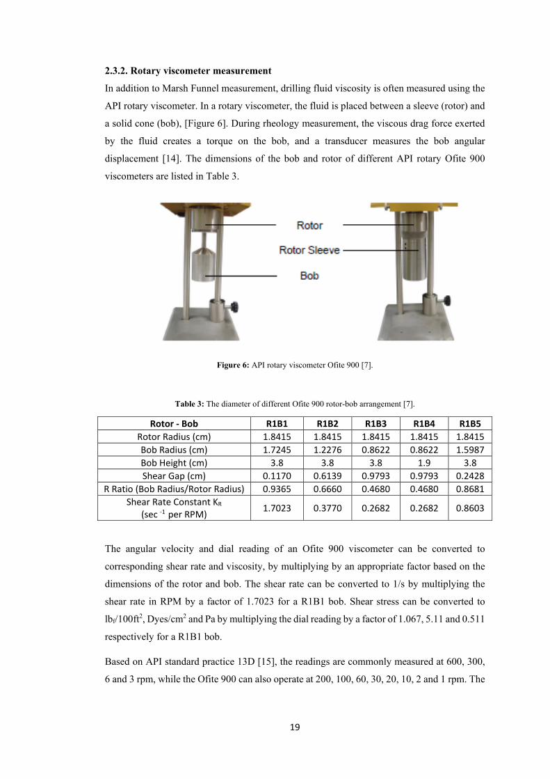
2.3.2. Rotary viscometer measurement
In addition to Marsh Funnel measurement, drilling fluid viscosity is often measured using the
API rotary viscometer. In a rotary viscometer, the fluid is placed between a sleeve (rotor) and
a solid cone (bob), [Figure 6]. During rheology measurement, the viscous drag force exerted
by the fluid creates a torque on the bob, and a transducer measures the bob angular
displacement [14]. The dimensions of the bob and rotor of different API rotary Ofite 900
viscometers are listed in Table 3.
Figure 6: API rotary viscometer Ofite 900 [7].
Table 3: The diameter of different Ofite 900 rotor-bob arrangement [7].
The angular velocity and dial reading of an Ofite 900 viscometer can be converted to
corresponding shear rate and viscosity, by multiplying by an appropriate factor based on the
dimensions of the rotor and bob. The shear rate can be converted to 1/s by multiplying the
shear rate in RPM by a factor of 1.7023 for a R1B1 bob. Shear stress can be converted to
lbf/100ft2, Dyes/cm2 and Pa by multiplying the dial reading by a factor of 1.067, 5.11 and 0.511
respectively for a R1B1 bob.
Based on API standard practice 13D [15], the readings are commonly measured at 600, 300,
6 and 3 rpm, while the Ofite 900 can also operate at 200, 100, 60, 30, 20, 10, 2 and 1 rpm. The
Rotor - Bob R1B1 R1B2 R1B3 R1B4 R1B5 Rotor Radius (cm) 1.8415 1.8415 1.8415 1.8415 1.8415 Bob Radius (cm) 1.7245 1.2276 0.8622 0.8622 1.5987 Bob Height (cm) 3.8 3.8 3.8 1.9 3.8 Shear Gap (cm) 0.1170 0.6139 0.9793 0.9793 0.2428
R Ratio (Bob Radius/Rotor Radius) 0.9365 0.6660 0.4680 0.4680 0.8681 Shear Rate Constant KR
(sec -1 per RPM) 1.7023 0.3770 0.2682 0.2682 0.8603

20
digital API rotary viscometers have more flexibility. The shear rate range of the Ofite 900
viscometer can be from 0.01 1/s to 1700 1/s when controlled by a programmed computer.
In addition to the API rotary viscometer, there are other rotary viscometers designed to
measure fluid properties in the lab. Two examples are the Brookfield and the HAAKE Mars
viscometers, [Figure 7].
Figure 7: Examples of other rotary viscometers: (a) Brookfield viscometer, (b) Haake Mars viscometer [7].
The Brookfield viscometer [16] is a rheology testing machine that provides both controlled
shear rate and controlled shear stress measurements and a variety of flow characterization tools
including ramp, loop and single point testings using specific spindles, [Figure 8][16]. The
application of the Brookfield viscosity measurement is mostly relevant for quality control and
benchmarking of additives and products.
Figure 8: Different spindle sets of Brookfield viscometer [16].
21
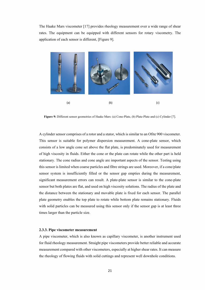
The Haake Mars viscometer [17] provides rheology measurement over a wide range of shear
rates. The equipment can be equipped with different sensors for rotary viscometry. The
application of each sensor is different, [Figure 9].
Figure 9: Different sensor geometries of Haake Mars: (a) Cone-Plate, (b) Plate-Plate and (c) Cylinder [7].
A cylinder sensor comprises of a rotor and a stator, which is similar to an Ofite 900 viscometer.
This sensor is suitable for polymer dispersion measurement. A cone-plate sensor, which
consists of a low angle cone set above the flat plate, is predominately used for measurement
of high viscosity in fluids. Either the cone or the plate can rotate while the other part is held
stationary. The cone radius and cone angle are important aspects of the sensor. Testing using
this sensor is limited when coarse particles and fibre strings are used. Moreover, if a cone/plate
sensor system is insufficiently filled or the sensor gap empties during the measurement,
significant measurement errors can result. A plate-plate sensor is similar to the cone-plate
sensor but both plates are flat, and used on high viscosity solutions. The radius of the plate and
the distance between the stationary and movable plate is fixed for each sensor. The parallel
plate geometry enables the top plate to rotate while bottom plate remains stationary. Fluids
with solid particles can be measured using this sensor only if the sensor gap is at least three
times larger than the particle size.
2.3.3. Pipe viscometer measurement
A pipe viscometer, which is also known as capillary viscometer, is another instrument used
for fluid rheology measurement. Straight pipe viscometers provide better reliable and accurate
measurement compared with other viscometers, especially at higher shear rates. It can measure
the rheology of flowing fluids with solid cuttings and represent well downhole conditions.

22
The schematic of a pipe viscometer is shown in Figure 10 [18]. The test fluid is circulated
through the pipeline with inner diameter D under pressure using a pump, and the friction
pressure drop (ΔP) across test section length ΔL and the flow rate (Q) are measured and
recorded by the Data Acquisition System (DAQ). The flow rate can be converted to actual
shear rate while pressure drop can be converted to actual shear stress, using the relationships
between parameters given below. The pipe viscometer is mostly used to measure the fluid
rheology at steady shear rates, i.e., it is not used to measure thixotropic properties.
Figure 10: Pipeline viscometer system [18].
To obtain reliable and accurate rheology measurement, the pipe viscometer should have a
sufficiently long entrance and exit section to ensure the fully developed flow condition is
established within the test section. Collins and Schowalter [19] proposed a correlation to
estimate the entrance length of the pipe XD for power law fluids as shown below,
XD = (−0.126n + 0.1752)D ∙ Re
(2.2)
where n, D and Re are the fluid behaviour index, pipe inner diameter and the Reynold number.
The pipe wall shear rate γ̇w and shear stress τw are defined as [20],
where u is the mean velocity, which is directly proportional to flow rate and inversely
proportional to the cross-section area of the pipe. 8uD
is termed as nominal Newtonian shear
rate. N is the generalized flow behaviour index, which is expressed as below,
γ̇w = �3N + 1
4N�
8uD
(2.3)

23
N =d(ln τw)
d �ln 8uD �
(2.4)
where τw is the shear stress at pipe wall surface and applies to both Newtonian and non-
Newtonian fluids,
τw =D4
×∆P∆L
(2.5)
Results from pipe viscometer tests [18] presented in Figure 11 show the plot of the average
wall shear stress as a function of nominal Newtonian shear rate for a test fluid, and this flow
curve can be used to screen out measurements that fall outside the laminar flow regime. The
wall shear stress increases sharply as the nominal shear rate increases in this area (the right-
side region of blue dashed line). In general, the wall shear stress in terms of nominal shear rate
can be also re-written as follows,
where K′ is the generalized consistency index, which is a function of nominal Newtonian shear
rate. If plotting the curve of τw versus 8u
D forms the straight line, then the fluid flowing in
the pipeline is a Power-Law fluid. If the fluid is Newtonian fluid, N=1 and then equation (2.3)
reduces to:
γ̇w =8uD
(2.7)
τw = K′ �8uD�N
(2.6)
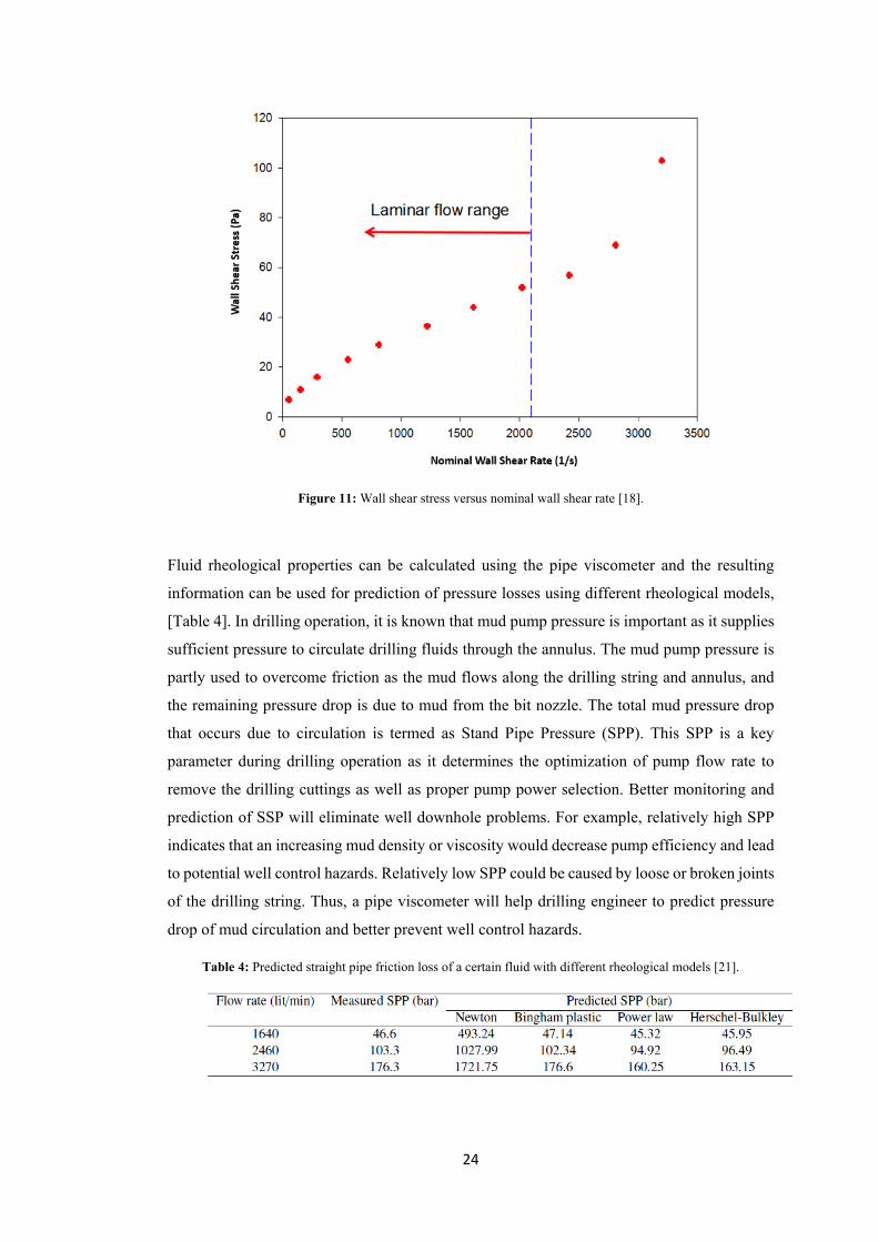
24
Figure 11: Wall shear stress versus nominal wall shear rate [18].
Fluid rheological properties can be calculated using the pipe viscometer and the resulting
information can be used for prediction of pressure losses using different rheological models,
[Table 4]. In drilling operation, it is known that mud pump pressure is important as it supplies
sufficient pressure to circulate drilling fluids through the annulus. The mud pump pressure is
partly used to overcome friction as the mud flows along the drilling string and annulus, and
the remaining pressure drop is due to mud from the bit nozzle. The total mud pressure drop
that occurs due to circulation is termed as Stand Pipe Pressure (SPP). This SPP is a key
parameter during drilling operation as it determines the optimization of pump flow rate to
remove the drilling cuttings as well as proper pump power selection. Better monitoring and
prediction of SSP will eliminate well downhole problems. For example, relatively high SPP
indicates that an increasing mud density or viscosity would decrease pump efficiency and lead
to potential well control hazards. Relatively low SPP could be caused by loose or broken joints
of the drilling string. Thus, a pipe viscometer will help drilling engineer to predict pressure
drop of mud circulation and better prevent well control hazards.
Table 4: Predicted straight pipe friction loss of a certain fluid with different rheological models [21].

25
2.4. Rheology measurement conditions
While fluid properties are measured at atmospheric condition, in reality the fluid is exposed to
elevated temperature and pressure during drilling operations. In the drilling string the fluid is
free of solids, but in the annulus, the fluid carries cuttings to surface, and therefore, the
presence of cuttings in the drilling fluid can influence fluid rheology. It is therefore important
to measure the fluid rheology at elevated temperature and pressure, and also at different solid
concentrations.
A review of the literature showed that the viscosity of water-based drilling fluid is very
dependent on the temperature and pressure [22]. High temperature and high pressure have a
significant impact on the fluid rheology, as shown by the variations of shear stress with shear
rate, at varying temperature or varying pressure, [Figure 12]. However, there is little research
on the rheological properties of drilling fluids over wide range of shear rates at very high
pressures/temperatures, which needs more investigation in the further study.
Figure 12: Effect of temperature and pressure on rheology of a certain fluid [22].
2.5. Influence of particles on drilling fluid rheology
The process of transporting rock cuttings from the drill bit through the annulus to the surface
is called cuttings transportation. The main factors affecting cutting transportation is the mud
rheology, borehole geometry and drilling fluid flow rate [23]. While the rheology of drilling
fluid is controlled by the composition of drilling fluid and wellbore temperature profile, the
solid particles in mud also have an impact on the drilling fluid rheology. The presence of solid
particles in the drilling fluid is associated with two factors: (a) the transportation of solid
particles in the annulus, which is associated with a wide range of solid particles and relative
high concentration of particles, and (b) the accumulated concentration of low-density solid
particles that cannot be removed from the drilling fluid [1].
26
The insoluble mud solids can be divided into two categories: high-gravity and low-gravity
solids. The concentration of high-gravity solids is minimized by the solid-control equipments
(from shale shaker to desander cone and the decanting centrifuge) after processing of the
drilling fluid at the surface. However, some solids are dispersed as fine particles, which cannot
be efficiently removed. As a result, the mud viscosity will be altered after re-circulation of
drilling fluid due to accumulation of low gravity solids. In this case, the drilling fluid must be
diluted with fresh mud containing no solid particles. However, the adding of zero solid fresh
mud will increase the mud cost dramatically and might affect the drilling fluid rheology, which
in turn affects the pumping efficiency. Currently, there are limited studies and experiments
with fine particles effect on rheology, which is ignored but it is very crucial for operation.
2.5.1. Solid particles in drilling fluid
Different types of solid particles found in drilling fluids include soluble material such as
Potassium Chloride (KCL) and insoluble fine/coarse drill cuttings and additives such as barite,
calcium carbonate or hematite.
The concentration of solid particles can be quantified using total solid content and total
suspended solid concentration. Total solid content is the percentage of the total solid in drilling
mud, which refers to soluble and insoluble solid content in the mud system. The total
suspended solid concentration is the weight fraction of the dry-weight of suspended particles
that are not dissolved in the suspending fluid.
The particle dispersion of suspensions can be divided into mono-dispersion and poly-
dispersion. Mono-dispersion refers to the particles of uniform size in a dispersed phase while
poly-dispersion, also known as disorder dispersion, refers to the particles of varied sizes in a
dispersed phase, [Figure 13] [24]. In the drilling industry, the coarse particles slightly influence
the bulk fluids viscosity but the fine cuttings are assumed to have significant impact on slurry
rheology, as shown in Figure 14.
Furthermore, cuttings transportation in drilling operation, becomes one of major factors
affecting drilling time and quality of well operation, which leads to pressure drop in circulating
flow [1].This phenomenon brings challenge for the drilling engineer to determine how the
cuttings affect pressure drop along the well annulus. Meanwhile, the accumulation of fine
cutting particles will increase drilling fluid density and finally affect equivalent drilling
circulating density, creating higher risk for well control procedures.

27
Figure 13: Monodisperse and poly-disperse suspensions with particles [24].
Figure 14: Properties of drilling fluids with different volume concentration of cuttings within same size [25].
2.5.2. Suspensions in drilling fluid
There has been extensive research focusing on characterising the impact of insoluble solids on
the drilling fluid rheology during medium and high shear rate regions [26]. Adding solid
particles to liquids changes the optical and physical properties of fluid. As the particles are
insoluble, the fluid is a two-phase/multi-phase mixture.
This two-phase/multi-phase mixture can form two types of systems depending on the settling
velocity of the particles. If the particles are suspended in the fluid and in a relatively long
period of time the particles will not settle, i.e. the particle settling velocity is regarded as zero,
the mixture is called as a suspension. Otherwise the mixture is unstable and usually referred
as slurry when the particle settling velocity is large enough.
Mud viscosity is difficult to measure in an unstable particle fast-settling system. The viscosity
of the suspending fluid is often not sufficiently high to suspend coarse drilling particles, and
as a result, the solid particles settle during rheology measurement, leading to inaccurate
measurements. For a suspension, the particles are generally fine or the suspending fluid has to
05
101520253035404550
1 2 3
Valu
es
Cutting Volume Concentration
Density
Specific gravity
Plastic viscosity
Yield point
Gel strength
pH

28
be viscous. To estimate whether the mixture is a suspension or not, it is necessary to predict
the particle settling velocity based on the properties of the fluid and particle such as the particle
size and fluid rheology. For a Newtonian fluid, Stokes’s law is used to calculate the particle
velocity for the laminar regime. But for the turbulent regime, the correlation of the particle
drag coefficient and Reynolds number is needed.
A low particle volume fraction might induce shear-thinning behaviour whereas high particle
volume fraction might result in shear-thickening [27]. Furthermore, in most suspensions, the
particle size distribution, particle shape and particle surface charge may alter the fluid rheology
as well, leading to more complex rheological behaviour in suspensions.
To avoid this source of error, this study will focus only on the stable suspensions in which the
particles are mono-sized and suspended by the viscous suspending fluid, so that the particles
will not settle down during measurements [28].
2.5.3. Effect of solid particles on fluid rheology
Here, a review of previous work studying the effect of solid particles on the fluid rheology is
summarized.
In various engineering disciplines, the relative viscosity ηr, which is the ratio between the
apparent viscosity of the suspension ηapp and the viscosity of the suspending fluid η0, is used
to quantify the fluid resistance to flow against shear rate [29].
Research by Rutgers et al [27] has addressed the parameters that affect the relative viscosity
of suspension fluids: (1) the volume fraction of the solid particles, (2) the type of suspended
particles and their shape and size, (3) the particle size distribution and (4) the shear rate
variation.
2.5.3.1. Effect of particle concentration on suspension viscosity
Previous research from Watanabe et al [30] showed that the suspension apparent viscosity
increases with the presence of solid particles. This study suggests that the apparent viscosity
increases with increasing solid concentration. This phenomenon is attributed to the enhanced
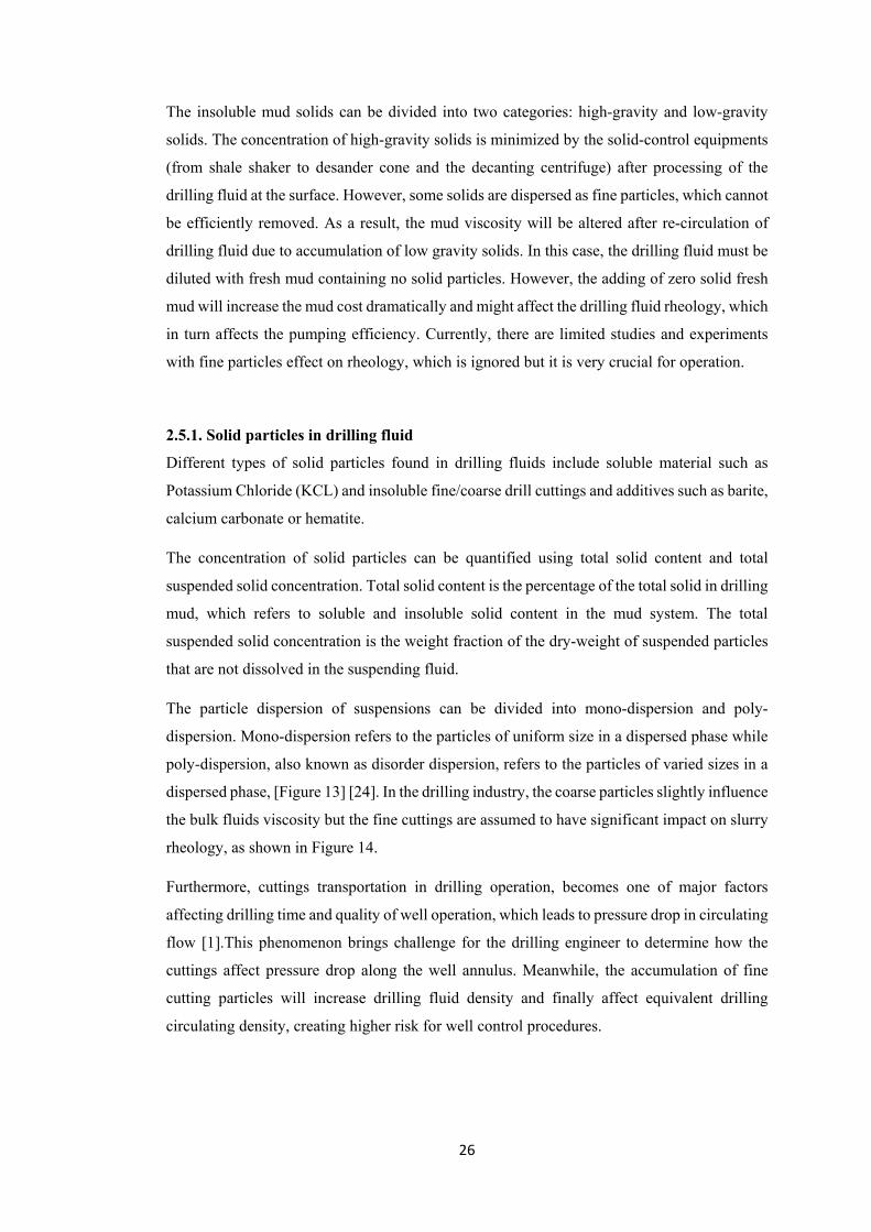
particle-particle interactions in the fluid, as shown in Figure 15. This contact between particles
increases particle frictional interaction, thereby increasing the apparent viscosity of
suspensions.
ηr = ηappη0
(2.8)
29
Figure 15: The impact of increasing particles concentration on the apparent viscosity of suspension [31].
2.5.3.2. Effect of particle size on suspension viscosity
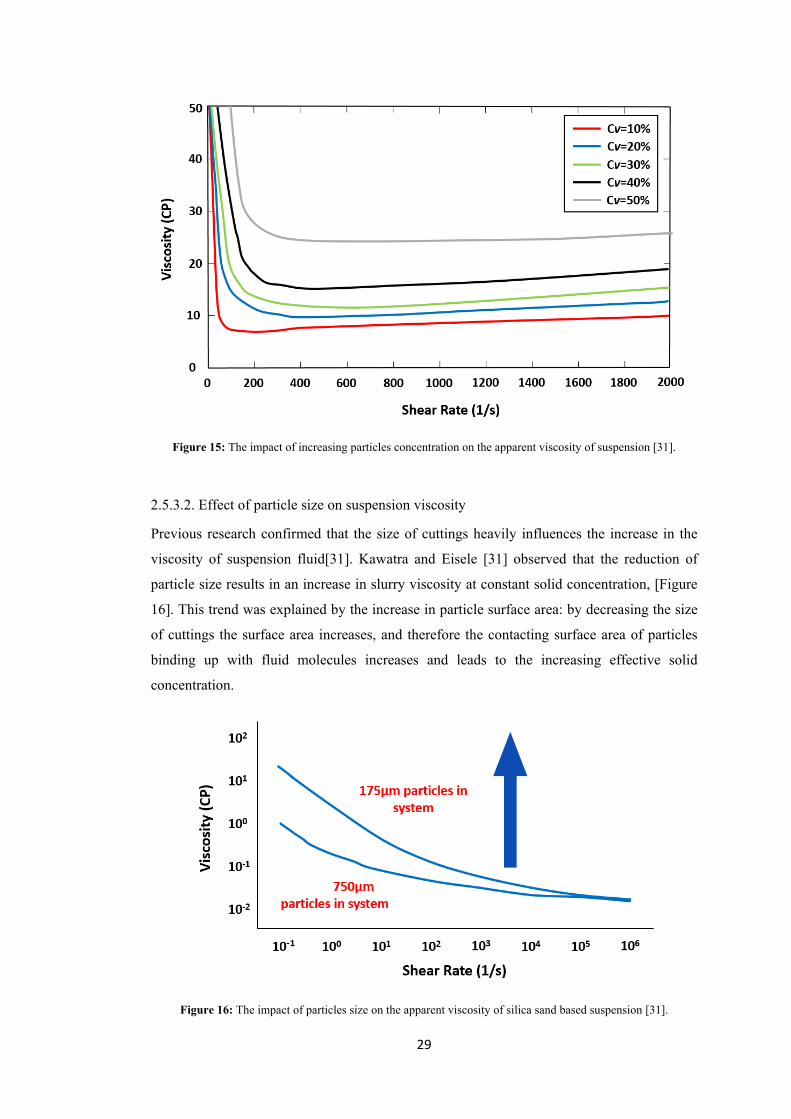
Previous research confirmed that the size of cuttings heavily influences the increase in the
viscosity of suspension fluid[31]. Kawatra and Eisele [31] observed that the reduction of
particle size results in an increase in slurry viscosity at constant solid concentration, [Figure
16]. This trend was explained by the increase in particle surface area: by decreasing the size
of cuttings the surface area increases, and therefore the contacting surface area of particles
binding up with fluid molecules increases and leads to the increasing effective solid
concentration.
Figure 16: The impact of particles size on the apparent viscosity of silica sand based suspension [31].

30
In contrast, the other research from Clark [31] showed the viscosity of suspension fluid
increases with the size of solid particles, as shown in Figure 17. This variation of viscosity
was attributed to the inertial effect resulting in additional energy dissipation, which increases
the viscosity of the suspension fluid.
Figure 17: The increase of suspension apparent viscosity by increasing particles size [31].
One explanation of this apparent contradiction is related to the effect of particle size on the
fluid viscosity - the microscopic structures of the suspended particles with different sizes are
very different. As shown Figure 18 in research conducted by S Mueller et al [32], the initial
state of the particle in suspension is characterized by the average size and fractal dimension of
the primary particles. Particles can easily form aggregates in low shear velocity conditions
with decreasing solid particles size, which results in the strongly entangled networks of
immobile particles. When the sample is sheared at medium or high shear rate, the flocculent
networks are broken up and the distance separating the fine particles increases and lowering
the attraction of particles.
Figure 18: The conceptual picture of agglomerated particles and chain structure particles [32].
31
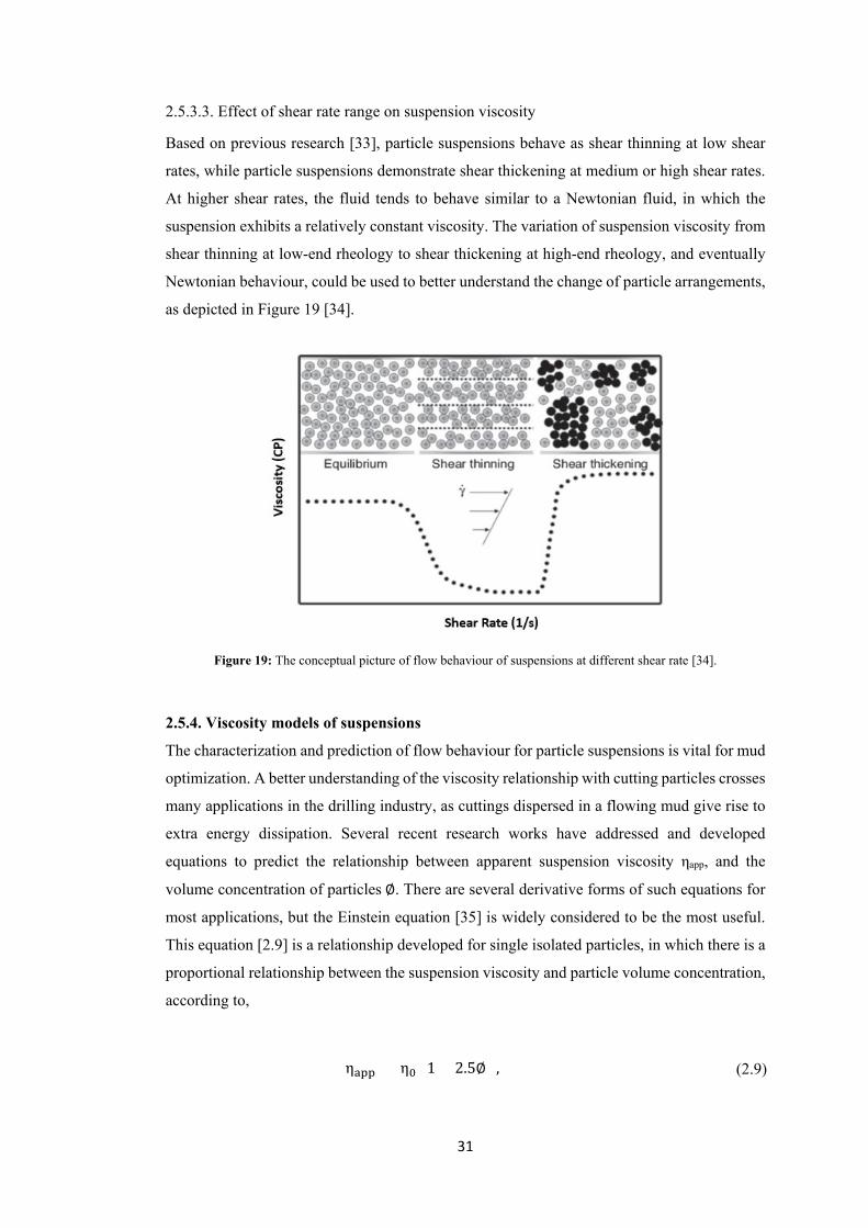
2.5.3.3. Effect of shear rate range on suspension viscosity
Based on previous research [33], particle suspensions behave as shear thinning at low shear
rates, while particle suspensions demonstrate shear thickening at medium or high shear rates.
At higher shear rates, the fluid tends to behave similar to a Newtonian fluid, in which the
suspension exhibits a relatively constant viscosity. The variation of suspension viscosity from
shear thinning at low-end rheology to shear thickening at high-end rheology, and eventually
Newtonian behaviour, could be used to better understand the change of particle arrangements,
as depicted in Figure 19 [34].
Figure 19: The conceptual picture of flow behaviour of suspensions at different shear rate [34].
2.5.4. Viscosity models of suspensions
The characterization and prediction of flow behaviour for particle suspensions is vital for mud
optimization. A better understanding of the viscosity relationship with cutting particles crosses
many applications in the drilling industry, as cuttings dispersed in a flowing mud give rise to
extra energy dissipation. Several recent research works have addressed and developed
equations to predict the relationship between apparent suspension viscosity ηapp, and the
volume concentration of particles ∅. There are several derivative forms of such equations for
most applications, but the Einstein equation [35] is widely considered to be the most useful.
This equation [2.9] is a relationship developed for single isolated particles, in which there is a
proportional relationship between the suspension viscosity and particle volume concentration,
according to,
ηapp = η0 (1 + 2.5∅) ,
(2.9)

32
where ηapp is apparent suspension viscosity, η0 is suspending medium fluid viscosity and ∅
is the volume fraction of the solid particles (assumed to be spherical). The volume fraction is
calculated from,
where V p and Vf denote the volumes of the particle and fluid phases respectively.
The Einstein equation is based on an idealized hard-sphere dispersion model system, as it
assumes that there is no any appreciable interaction between the solids, and that all particles
are single and isolated. This equation is only applicable for diluted dispersions of spherical
particles which volume concentration is less than 1% (∅ < 0.01) [35].
It can be summarised from the Einstein equation that the viscosity of dispersions mainly
depends on the volume concentration of suspended particles and it is a linear function of the
particle volume fraction [35]. Although the Einstein equation is limited to rigid and spherical
particles, actual experiment conditions can differ considerably from these theoretical
assumptions. For higher particle concentration, multi-particle interaction becomes important
and it has to be taken accounted. Thus, numerous empirical corrections have been developed
to calculate viscosity of suspensions under this circumstance [35].
Krieger-Dougherty [36] suggested a semi-empirical equation, which is applicable for a wide
concentration range of suspensions and better fitted to highly concentrated suspension
rheology measurements,
ηr = (1 −∅∅m
)−[η] ∅m ,
(2.11)
where ∅𝑚𝑚 is the maximum packing fraction or volume fraction of the suspension [29]. The
absolute value of the latter is determined by particle packing geometry, which only depends
on particle shape and size distribution [37]. It should be mentioned, that particles would realign
in the flow direction, which causes more efficient packing rather than random packed structure
at rest, so the maximum packing fraction has different value from low shear rate to high shear
rate. [η] referred as the ‘Einstein coefficient’ or ‘intrinsic viscosity’ and takes the value of 2.5
for spherical particles [38]. However, there is no unique value of intrinsic viscosity as this
parameter differs with different suspensions. This particle interaction coefficient increases
with the increasing number of fine particles in the suspensions [39].
∅ = V p
Vf + Vp , (2.10)
33
A similar equation suggested by Quemada et al [40] can also be applied for calculation of
relative viscosity over a wider range of concentrations rather than original Einstein equation:
However, not one simple model can describe solid-particle relationships perfectly from very
dilute to highly concentrated states as particle in a suspending medium can be subject to
hydrodynamic interaction, Brownian motion and well as other effects.
The current literature does not provide enough data for particle suspensions from low-end to
high-end shear rates. Little comprehensive work and systematic studies have been done for
polymer drilling fluids with fine suspended cuttings. As part of the proposed study,
investigations will focus on how the cutting particles alter the rheology of polymer drilling
fluids and the effect on thixotropic behaviour.
2.6. Polymer synergy
During drilling operation, the drilling fluid is required to have high low-end viscosity. As the
drilling fluid moves through the upward section of larger annulus, the fluid velocity decreases,
which results in smaller carrying capacity. In order to carry the cuttings to the surface, it is
essential for the drilling fluid to exhibit high viscosity at lower shear rate to compensate for
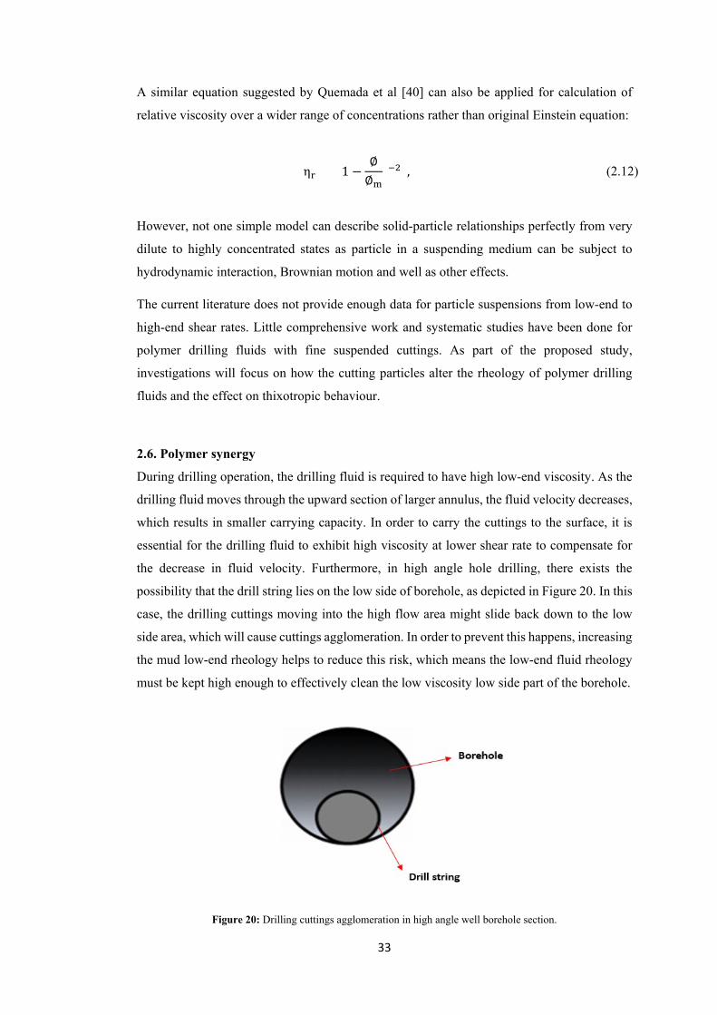
the decrease in fluid velocity. Furthermore, in high angle hole drilling, there exists the
possibility that the drill string lies on the low side of borehole, as depicted in Figure 20. In this
case, the drilling cuttings moving into the high flow area might slide back down to the low
side area, which will cause cuttings agglomeration. In order to prevent this happens, increasing
the mud low-end rheology helps to reduce this risk, which means the low-end fluid rheology
must be kept high enough to effectively clean the low viscosity low side part of the borehole.
Figure 20: Drilling cuttings agglomeration in high angle well borehole section.
ηr = (1 −∅∅m
)−2 ,
(2.12)
34
Research on the low-end rheological modifiers and their synergistic optimization is a major
area for improvement in the drilling industry. Low-end rheology refers to the rheology at the
almost zero constant shear rate. The shear rate of flowing drilling fluid tends to be less than
100 1/s at the wall of the borehole while nearly approaching zero in the centre of annulus.
Xanthan Gum is a low-shear-rate rheological booster widely used in the field, as it has high
viscosity at low shear rate. The structure of Xanthan Gum and its properties are summarized
in Table 5 [41]. Compared with other common gums over a range of shear rates, Xanthan Gum
has approximately 15 times the viscosity of Guar Gum or CMC at very low shear rate [41]. In
this case, determination of the optimal combination between Xanthan Gum and other gums is
very crucial for drilling operation, for a lower cost of drilling mud and production of better
rheology from low-end to high-end.
Synergetic interaction refers to the effect of two or more chemicals, together, being greater
than the theoretical combination of each polymer. In drilling operation, drilling fluid with
extensive shear thinning property is highly desired. High viscosity at low shear rate is desired
to control the fluid loss in unconsolidated and fractured formations. Low viscosity at high
shear rate is desired for minimising the pressure drop in the coiled tube, drill string, downhole
tools and annulus, which in turn increasing the efficiency of drilling pump during operation.
Furthermore, having low-viscosity at high shear rates improves solid removal efficiency using
hydrocyclone and centrifuge decanters.
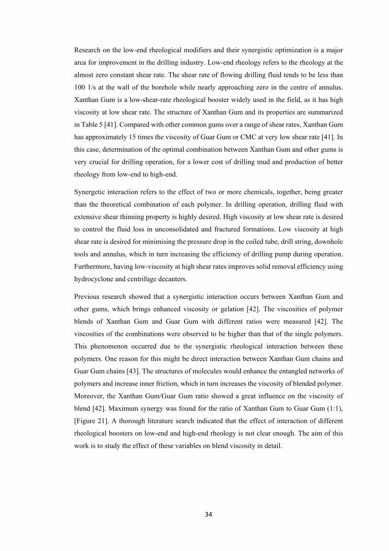
Previous research showed that a synergistic interaction occurs between Xanthan Gum and
other gums, which brings enhanced viscosity or gelation [42]. The viscosities of polymer
blends of Xanthan Gum and Guar Gum with different ratios were measured [42]. The
viscosities of the combinations were observed to be higher than that of the single polymers.
This phenomenon occurred due to the synergistic rheological interaction between these
polymers. One reason for this might be direct interaction between Xanthan Gum chains and
Guar Gum chains [43]. The structures of molecules would enhance the entangled networks of
polymers and increase inner friction, which in turn increases the viscosity of blended polymer.
Moreover, the Xanthan Gum/Guar Gum ratio showed a great influence on the viscosity of
blend [42]. Maximum synergy was found for the ratio of Xanthan Gum to Guar Gum (1:1),
[Figure 21]. A thorough literature search indicated that the effect of interaction of different
rheological boosters on low-end and high-end rheology is not clear enough. The aim of this
work is to study the effect of these variables on blend viscosity in detail.
35
Table 5: Structure and property relationship of Xanthan Gum [43].
Figure 21: Viscosity synergism between Xanthan Gum and Guar Gum [42].

36
Chapter 3. Methodology
3.1. Introduction
This chapter introduces the methodology for measurement of the rheology, over a wide range
of shear rates, for different polymers and bentonite. The methodology for testing different
combinations of polymers, leading to a blend that can yield extensive shear thinning behaviour
with elevated viscosity at low shear rate, will also be detailed. At last, the experiment to study
the effect of solid particles on suspension solutions is illustrated.
3.2. Rheological measurement
3.2.1. Ofite measurement
A 12-speed Ofite 900 viscometer with R1B1 bob and rotor arrangement was used for synergy
experiments [Figure 22]. The aim of the experiments was to validate functions of different
viscosity boosters and their differences in enhancing low-end rheology. They were dissolved
in water at room temperature and stirred at 1000rpm, using an overhead mixer. For the purpose
of fluid hydration, the mixing time was maintained at a minimum of 20 minutes and then later
measured by Ofite 900 R1B1 viscometer. Then the weight concentrations of additives were
adjusted to ensure they had very similar dial readings at an angular velocity of 600 rpm, which
corresponded to a shear rate of 1021.24 1/s. This shear rate, and that of 510.69 1/s
(corresponding to 300 rpm) are the main shear rates used in petroleum engineering for
viscosity measurement [1]. Finally, Haake Mars viscometer was used for step-wise rheological
measurement.
Figure 22: Ofite 900 viscometer with R1B1 geometry.

37
3.2.2. Haake measurement
3.2.2.1. Haake step-wise test
A specific step-wise shear profile was performed using the Haake Mars viscometer with Z20
DIN sensor geometry, to measure viscosity of a test sample for synergy experiments.
According to the instruction manual, 8.2ml of test sample was placed into the cylinder chamber
and step-wise shear rates were applied. Various shear rates were applied starting from a low
shear rate of 0.1 1/s to a high shear rate of 1900 1/s. At low shear rates, the duration of exposure
was 3 minutes, while the duration of exposure for medium and high shear rates was 30 seconds.
The corresponding viscosity was obtained with the variation of shear rates. The Haake
RheoWin3 software was used to plot shear stress versus shear rate, and viscosity versus shear
rate relation of suspensions in real-time during measurement [Figure 23].
Figure 23: Haake RheoWin 3 interface-real time graph.
The effect of cuttings on suspension was also investigated using the Haake Mars viscometer.
High viscosity suspending fluid was used to minimise the particle settlement during the
experiments, and different sizes and concentrations of particles were used. The suspensions
with particles were sheared before the viscosity measurement. This “pre-shear” condition was
applied to ensure suspended particles are randomly oriented and that equilibrium orientation
distributions were established. After a period of shearing, the Haake step-wise experiment was
conducted [Figure 24]. The experimental temperature was set at 25 ℃.

38
Figure 24: MATLAB analysis of Haake step-wise measurement of one suspension with particles.
3.2.2.2. Haake thixotropic loop test
A thixotropic loop test was conducted under shear-controlled conditions to quantify the
thixotropic behaviour of a test sample, as shown in Figure 25. In this test, the test sample was
pre-sheared to thoroughly break down any existing structure and allow a rest period to rebuild
the structure of the sample. The shear rate was then ramped up from zero shear rate to a
maximum of 1900 1/s in 100 seconds and held constant for 80 seconds. It was then ramped
smoothly from 1900 1/s back to zero shear rate in 100 seconds.
Figure 25: Example of the variation of shear rate with time during a thixotropic loop test of suspension.
0200400600800
100012001400160018002000
0 50 100 150 200 250 300
Shea
r Rat
e (1
/s)
Time (s)
39
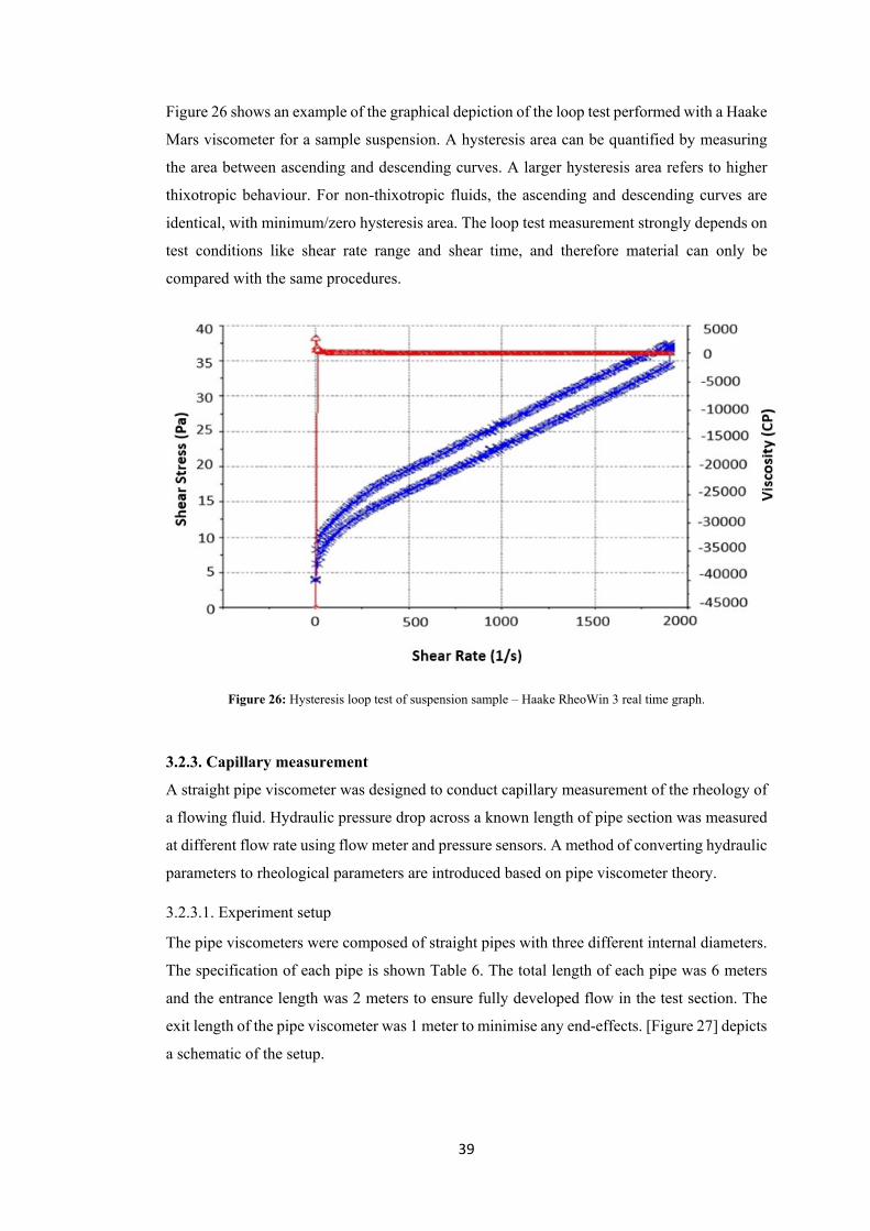
Figure 26 shows an example of the graphical depiction of the loop test performed with a Haake
Mars viscometer for a sample suspension. A hysteresis area can be quantified by measuring
the area between ascending and descending curves. A larger hysteresis area refers to higher
thixotropic behaviour. For non-thixotropic fluids, the ascending and descending curves are
identical, with minimum/zero hysteresis area. The loop test measurement strongly depends on
test conditions like shear rate range and shear time, and therefore material can only be
compared with the same procedures.
Figure 26: Hysteresis loop test of suspension sample – Haake RheoWin 3 real time graph.
3.2.3. Capillary measurement
A straight pipe viscometer was designed to conduct capillary measurement of the rheology of
a flowing fluid. Hydraulic pressure drop across a known length of pipe section was measured
at different flow rate using flow meter and pressure sensors. A method of converting hydraulic
parameters to rheological parameters are introduced based on pipe viscometer theory.
3.2.3.1. Experiment setup
The pipe viscometers were composed of straight pipes with three different internal diameters.
The specification of each pipe is shown Table 6. The total length of each pipe was 6 meters
and the entrance length was 2 meters to ensure fully developed flow in the test section. The
exit length of the pipe viscometer was 1 meter to minimise any end-effects. [Figure 27] depicts
a schematic of the setup.

40
A differential pressure transmitter, an absolute pressure transmitter and a flow meter were
installed on the pipeline to measure the friction drop of fluid flowing through the test section
and the volumetric flow rate during experiments.
A detailed description of the apparatus is presented below.
Table 6: Specification of pipe viscometers.
External diameter (inch)
Internal diameter
(inch)
Entrance length (m)
Exit length (m)
Typical flow rate (lpm)
0.5 0.43 2 1 4.42-19.47 0.75 0.62 2 1 4.54-25.96
1 0.87 2 1 2.48-25.27
Figure 27: Straight pipe viscometer.
Siemens Sitrans FM Mag 5000 and SITRANS F M TRANSMAG 2 flow meters were both
used for flow rate measurements, [Figure 28].The Siemens Sitrans FM Mag 5000 is a
microprocessor-based transmitter engineered for high performance. However, the
disadvantage encountered with this flowmeter is that it cannot measure flow rate reading
correctly below 10 litre per minutes. SITRANS F M TRANSMAG 2 is used instead to measure
the flow rate at lower range. It has better accuracy at low flow rate.
Figure 28: SIEMENS flow transmitter FM Mag 5000 and SITRANS F M TRANSMAG 2.
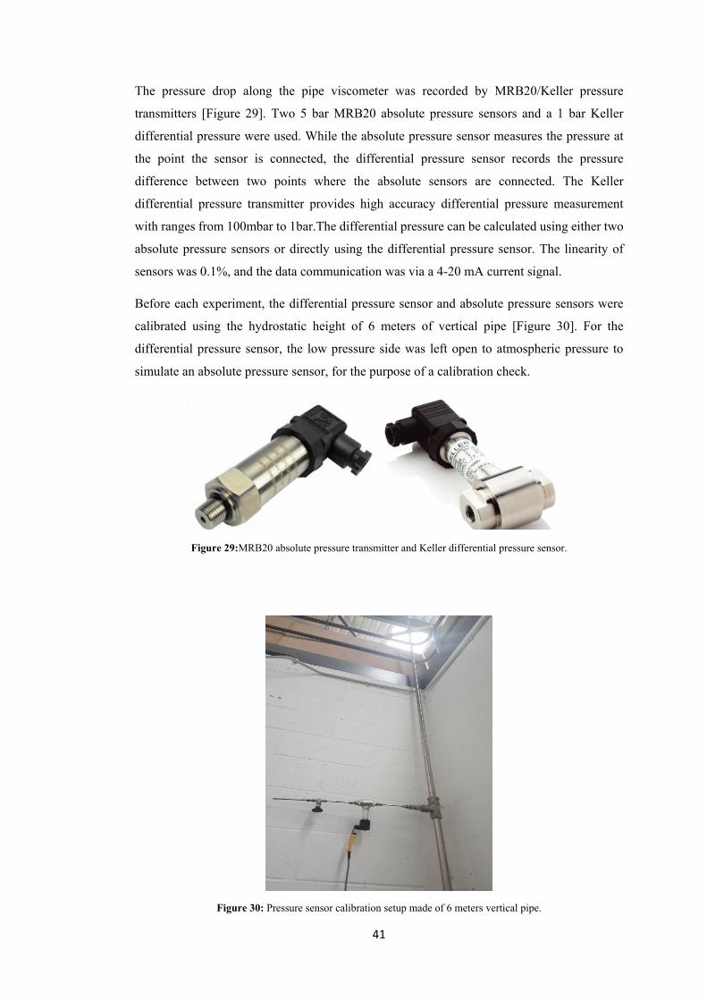
41
The pressure drop along the pipe viscometer was recorded by MRB20/Keller pressure
transmitters [Figure 29]. Two 5 bar MRB20 absolute pressure sensors and a 1 bar Keller
differential pressure were used. While the absolute pressure sensor measures the pressure at
the point the sensor is connected, the differential pressure sensor records the pressure
difference between two points where the absolute sensors are connected. The Keller
differential pressure transmitter provides high accuracy differential pressure measurement
with ranges from 100mbar to 1bar.The differential pressure can be calculated using either two
absolute pressure sensors or directly using the differential pressure sensor. The linearity of
sensors was 0.1%, and the data communication was via a 4-20 mA current signal.
Before each experiment, the differential pressure sensor and absolute pressure sensors were
calibrated using the hydrostatic height of 6 meters of vertical pipe [Figure 30]. For the
differential pressure sensor, the low pressure side was left open to atmospheric pressure to
simulate an absolute pressure sensor, for the purpose of a calibration check.
Figure 29:MRB20 absolute pressure transmitter and Keller differential pressure sensor.
Figure 30: Pressure sensor calibration setup made of 6 meters vertical pipe.

42
The DAQ SomatXR MX840B-R data acquisition system is used for this experiment, to record
and digitise the signals [Figure 31]. Catmaneasy is the software interface used for data
acquisition, which provides real-time display of data during the experiment, and enables
saving the data in MATLAB format for further processing, [Figure 32]. All recorded data is
later processed using a MATLAB code and presented in an Excel spreadsheet.
Figure 31: DAQ SomatXR MX840B-R data acquisition system.
Figure 32: CatmanEasy Interface– real time graph.
3.2.3.2. Bias test
According to experimental procedures, air bubbles along the pipeline were released to
minimize the effect air entrainment and bias measurement conducted prior to each experiment.
Figure 33 illustrates the variation of sensor bias of pressure sensors during an experiment. For
the bias test, all the valves along the pipe viscometer were closed to ensure that the fluid inside
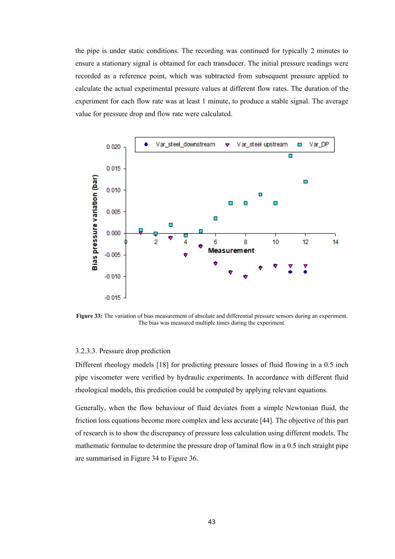
43
the pipe is under static conditions. The recording was continued for typically 2 minutes to
ensure a stationary signal is obtained for each transducer. The initial pressure readings were
recorded as a reference point, which was subtracted from subsequent pressure applied to
calculate the actual experimental pressure values at different flow rates. The duration of the
experiment for each flow rate was at least 1 minute, to produce a stable signal. The average
value for pressure drop and flow rate were calculated.
Figure 33: The variation of bias measurement of absolute and differential pressure sensors during an experiment. The bias was measured multiple times during the experiment.
3.2.3.3. Pressure drop prediction
Different rheology models [18] for predicting pressure losses of fluid flowing in a 0.5 inch
pipe viscometer were verified by hydraulic experiments. In accordance with different fluid
rheological models, this prediction could be computed by applying relevant equations.
Generally, when the flow behaviour of fluid deviates from a simple Newtonian fluid, the
friction loss equations become more complex and less accurate [44]. The objective of this part
of research is to show the discrepancy of pressure loss calculation using different models. The
mathematic formulae to determine the pressure drop of laminal flow in a 0.5 inch straight pipe
are summarised in Figure 34 to Figure 36.

44
Figure 34: Pressure drop equation of Bingham plastic model fluid, summarised from [18].
Figure 35: Pressure drop equation of Power law model fluid, summarised from [18].
Figure 36: Pressure drop equation of H-B model fluid, summarised from [18].

45
3.3. Test material
3.3.1. Additives
3.3.1.1. Additives for synergy experiments
The viscosifiers, used in synergy experiments are, Guar Gum, Pac-R, Aus-Gel-Xtra , Corewell
and Xanthan Gum, which are ideal for viscosity enhancement due to their low cost and
resistance to thermal degradation. However, there may be differences in their capability to
increase low-end rheology.
Guar Gum is a white powder manufacturing from guar beans, which widely used as a
stabilizing, thickening and suspending agent in the drilling industry. The disadvantage of Guar
Gum is its sensitivity to high pH. Pac-R is a filtration control additive, which is mostly used
in water-based mud. It helps to control filtration rate and provide supplementary viscosity in
fresh water, seawater and brine-based fluids. Aus-Gel-Xtra is a modified premium grade
Wyoming bentonite which used as a high yielding viscosifier with excellent wellbore cleaning
properties. Corewell is a dispersible product which is used to protect exposed formation during
drilling operation. Xanthan Gum is a natural white powder, which can dissolve readily in water
and thicken the drilling mud.
3.3.1.2. Additives for particle effect experiments
In order to minimise solids settling during the tests and to better characterise the cutting effect
on drilling fluid, an aqueous solution of 0.5 wt. % Xanthan Gum was used as suspending fluid.
The concentration and type of polymer is particular selected to provide sufficient viscosity to
suspend the sand and calcium carbonate particles and to create a nearly stable suspension
during experiment. In this research, Xanthan Gum was supplied from Australian Mud
Company (AMC) under commercial name of XanboreTM, [Figure 37].
To prepare 0.5 wt. % fluid, XanboreTM was completely mixed with water. Xanthan Gum
powder was slowly added to distilled water and agitated at 1000 rpm for 20 minutes. Poor
dispersion leads to clumping of particles (known as “fish eyes”) and reduces chemical
functionality.
46
Figure 37: AMC Xanthan Gum (XanboreTM) of suspending fluid.
3.3.1.3. Additives for pipe viscometer experiments
An aqueous solution of 6 wt. % bentonite was used for the capillary measurement to study its
rheology effect on the friction loss along the straight pipe viscometer. Bentonite is a natural
clay mineral most widely used in the water base drilling fluid, and functions as a lubricant and
coolant for the drill bit. It helps remove cuttings and prevents blowouts. Bentonite solution
was chosen for experiment as it tends to provide a more stable fluid viscosity. Unlike other
viscosifier additives such as polymers, it is not affected by bacteria activity or previous shear
history. Bentonite fluid was prepared in an industrial tank with capacity of 1000 litres using
high-speed agitator, [Figure 38].
Figure 38 : The storage tank with the agitator.

47
3.3.2. Solid particles
The particle effect experiments were performed using graded sands and Calcium Carbonate
particles suspended in Xanthan Gum fluid to form solid-liquid suspensions. Narrow particle
size ranges were selected using sieving method – the sieves and the sieve shaker are shown in
Figure 39. Three size ranges of sand particles, and one size range of Calcium Carbonate
particles were physically sorted using the sieving method. The details of particles are shown
in Table 7.
The fine particles weight concentrations in the suspension ranged starting from 1 wt. % to 10
wt. %, to create a diluted to concentrated solid suspensions. As the average densities of fine
particles are 2. 65 g/cm3, the corresponding particle volume concentrations ranged from 0.3
vol. % to 3 vol. %. Higher angular velocities of the mixer were avoided to minimise formation
of air bubbles in the suspension, and to obtain homogeneous monodisperse suspensions. The
effect of particle shape was not studied in this research due to the difficulties associated with
supplying solid particles with different shapes.
Figure 39: Sieve shaker (left) and sieve meshes (right) for 200 μm, 150 μm, 106 μm, and 75 μm (top to bottom).

48
Table 7: Size range of solid particles.
Particle Particle Size
(microns)
Solid Concentration
(wt. %)
Solid Concentration
(vol. %)
Calcium Carbonate 38-75
0.3 1 0.9 3 1.5 5 2.4 8 3.0 10
Silica Sand
106-200
0.3 1 0.9 3 1.5 5 2.4 8 3.0 10
200-250
0.3 1 0.9 3 1.5 5 2.4 8 3.0 10
250-300
0.3 1 0.9 3 1.5 5 2.4 8 3.0 10

49
Chapter 4. Results and Discussion Experimental results along with the interpretation are presented below.
4.1. Benchmarking of different rheology measurement techniques
In order to investigate the reliability of the Marsh Funnel as a qualitative measurement of fluid
rheology, a particular comparison experiment, also termed ‘the benchmark experiment’, was
designed. The Marsh Funnel and API rotary viscometer were used to determine rheological
properties of drilling fluids. Two drilling fluid solutions were made using bentonite and a
nature polymer Pac-R. The concentration of the Pac-R was adjusted to produce a similar Marsh
Funnel viscosity as the bentonite mud system. The Marsh Funnel viscosity was 81s for the
bentonite mud and 81.5s for the polymer mud. The samples were also tested using the Ofite
R1B1 viscometer, and the rheology measurements are illustrated in Figure 40.
As observed in the Figure 40, these two fluids might be similar at particular shear rates, but
indeed they had distinctive properties, and therefore different responses in drilling. However,
if the measurement using the Marsh Funnel was only considered, both fluids were expected to
produce similar fluid response (e.g. in the case of pressure drop or cutting transportation).
Figure 40: Comparison of fluid viscosity of a polymer and a bentonite solution using Ofite 900 R1B1 rotary viscometer.
Different sensors can be used for a particular rotary viscometer equipment. There is a lack of
literature evidence to investigate the effect of sensor type on the rheological measurement. As
part of this study, a controlled experiment was devised to evaluate if the measurements from
different sensors [Figure 41] are in agreement. In order to evaluate different rotary viscometry
0
10
20
30
40
50
60
0 200 400 600 800 1000 1200
Shea
r Str
ess (
Pa)
Shear Rate (1/s)
Natural Polymer
Bentonite

50
test methods, a 0.3 wt. % Xanthan Gum solution was selected and tested using a Haake Mars
rotational viscometer. The concentration and type of polymer were selected in order to achieve
high low-end rheology so that any potential inconsistency in measurement due to low values
of viscosity would be minimal, and the effect of sensor can be obtained more accurately. Three
sensors used in Haake Mars viscometers, namely cylinder sensor Z20DIN, plate-plate sensor
PP35Ti and cone-plate sensor C35/4Ti, were used [Table 8].
Figure 41: Haake Mars Z20DIN, PP35Ti and C35/4Ti sensor systems.
Table 8: Specification of Haake Mars sensor systems.
Sensor Cylinder-Z20DIN Cone-Plate-C35/4TI Plate-Plate-PP 35TI Maximum Shear Rate 1900 1/s 2249 1/s 2749 1/s
Sample Volume 8.20 cm3 0.80 cm3 0.80 cm3 Gap 0.85 mm 0.14 mm 1.00 mm
Angle 0 ° 4 ° 0 ° Clearance to Bottom 4.20 mm / /
Figure 42 showed the measured viscosity from Haake Mars viscometer, using different sensors,
by varying the shear rates. It shows that measurements with different sensor geometries are
closer to each other at medium and high shear rate ranges. Across the range of shear rates, the
cylinder sensor measures up to 1900 1/s while plate-plate sensor can measure up to 2749 1/s
and the cone-plate can measure up to 2249 1/s. These three sensor systems meet rheology
measurement requirements across a very wide shear range. However, the main disadvantage
of the plate-plate and cone-plate sensors is that test fluid can evaporate easily during
measurement, and that the sensors are not suitable to measure suspensions with particles. The

51
cylinder sensor Z20 DIN (bob diameter = 20mm and inner cup diameter =21.7mm, gap
4.20mm) was used for thixotropic loop measurements and rheological measurement of
suspension with particles during this research.
Figure 42: Rheological measurement of 0.3 wt. % Xanthan Gum measuring with different geometries of Haake Mars.
The Ofite R1B1 viscometer is commonly used in petroleum engineering, while the Ofite R1B2
can be used when more accurate measurement of viscosity at low shear rates is required. The
measurements of typical viscometer and advanced Haake Mars are in agreement at specific
shear rate. To compare these two rheological measurements, a benchmark experiment was
conducted with a fluid mixture of 0.18 wt. % Xanthan Gum and 0.02 wt. % Guar Guam, to
achieve high viscosity at low shear rate. A log plot of viscosity versus shear rate as shown in
Figure 43 suggests that the measurements are similar for different viscometers over the point
of 1.7 1/s, however, the typical viscometer Ofite 900 cannot measure very low-end or high-
end rheology. Similar comparison experiments were also carried out with other low-end
rheology viscosifiers, which suggested the Ofite 900 and Haake Mars are in agreement during
measurement over a wide shear range applicable to drilling fluids.

52
Figure 43: Comparison of rheological measurements with Haake Z20DIN, Ofite R1B1 and R1B2 geometries.
For the rheological measurement of flowing fluid, a straight pipe viscometer is an industrially
accepted apparatus. The pressure drop measurements of 6 wt. % bentonite are shown in Figure
44. This measurement was first conducted with 0.5 inch straight pipe viscometer of internal
diameter 0.4299 inch. The pressure drop was calculated by comparing the absolute pressure
measurements of two 5 bar MRB20 absolute pressure sensors and also directly measured using
the 1 bar Keller differential pressure sensor. To determine the rheological parameters and
compare with the Ofite 900 viscometer rheological measurements, the wall shear stress and
corresponding value of the flow characteristic were calculated. The analysis of the 0.5 inch
pipe viscometer data is presented in Table 9.
Figure 44: MATLAB interface of pressure drop experiment of 0.5 inch straight pipe viscometer.
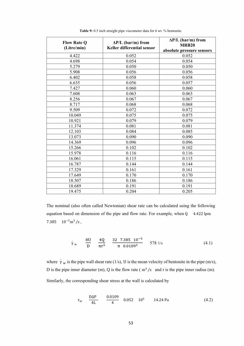
53
Table 9: 0.5 inch straight pipe viscometer data for 6 wt. % bentonite.
Flow Rate Q (Litre/min)
ΔP/L (bar/m) from Keller differential sensor
ΔP/L (bar/m) from MRB20
absolute pressure sensors 4.422 0.052 0.052 4.698 0.054 0.054 5.279 0.050 0.050 5.908 0.056 0.056 6.402 0.058 0.058 6.635 0.056 0.057 7.427 0.060 0.060 7.608 0.063 0.063 8.256 0.067 0.067 8.717 0.068 0.068 9.509 0.072 0.072
10.049 0.075 0.075 10.921 0.079 0.079 11.374 0.081 0.081 12.103 0.084 0.085 13.073 0.090 0.090 14.369 0.096 0.096 15.266 0.102 0.102 15.978 0.116 0.116 16.061 0.115 0.115 16.787 0.144 0.144 17.329 0.161 0.161 17.649 0.170 0.170 18.507 0.186 0.186 18.689 0.191 0.191 19.475 0.204 0.205
The nominal (also often called Newtonian) shear rate can be calculated using the following
equation based on dimension of the pipe and flow rate. For example, when Q = 4.422 lpm =
7.385 × 10⁻⁵m3 /s ,
where γ ̇ w is the pipe wall shear rate (1/s), U is the mean velocity of bentonite in the pipe (m/s),
D is the pipe inner diameter (m), Q is the flow rate ( m3 /s ) and r is the pipe inner radius (m).
Similarly, the corresponding shear stress at the wall is calculated by
γ ̇ w = 8UD
= 4Qπr3
= 32×7.385×10−5
π×0.01093 = 578 1/s
(4.1)
τw = D∆P 4L
= 0.0109
4× 0.052 × 105 = 14.24 Pa
(4.2)
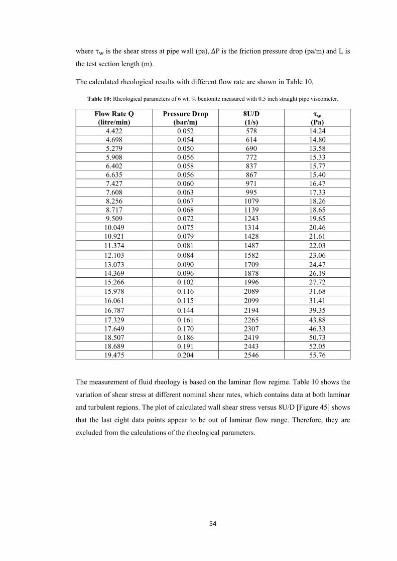
54
where τw is the shear stress at pipe wall (pa), ∆P is the friction pressure drop (pa/m) and L is
the test section length (m).
The calculated rheological results with different flow rate are shown in Table 10,
Table 10: Rheological parameters of 6 wt. % bentonite measured with 0.5 inch straight pipe viscometer.
Flow Rate Q (litre/min)
Pressure Drop (bar/m)
8U/D (1/s)
𝛕𝛕𝐰𝐰 (Pa)
4.422 0.052 578 14.24 4.698 0.054 614 14.80 5.279 0.050 690 13.58 5.908 0.056 772 15.33 6.402 0.058 837 15.77 6.635 0.056 867 15.40 7.427 0.060 971 16.47 7.608 0.063 995 17.33 8.256 0.067 1079 18.26 8.717 0.068 1139 18.65 9.509 0.072 1243 19.65
10.049 0.075 1314 20.46 10.921 0.079 1428 21.61 11.374 0.081 1487 22.03 12.103 0.084 1582 23.06 13.073 0.090 1709 24.47 14.369 0.096 1878 26.19 15.266 0.102 1996 27.72 15.978 0.116 2089 31.68 16.061 0.115 2099 31.41 16.787 0.144 2194 39.35 17.329 0.161 2265 43.88 17.649 0.170 2307 46.33 18.507 0.186 2419 50.73 18.689 0.191 2443 52.05 19.475 0.204 2546 55.76
The measurement of fluid rheology is based on the laminar flow regime. Table 10 shows the
variation of shear stress at different nominal shear rates, which contains data at both laminar
and turbulent regions. The plot of calculated wall shear stress versus 8U/D [Figure 45] shows
that the last eight data points appear to be out of laminar flow range. Therefore, they are
excluded from the calculations of the rheological parameters.

55
Figure 45: Wall shear stress versus nominal shear rate.
The data points are then presented in a logarithmic plot of wall shear stress versus nominal
shear rate to establish a relation between the flow behaviour N and 8U/D . A polynomial
trendline is fitted to the data as shown in Figure 46. The flow behaviour N = 2 ×
0.2715 ln �8UD� − 3.2292 according to equation (2.4). After obtaining N for different shear
rates, the corresponding true wall shear rate γ̇w can be calculated according to equation (2.3),
as shown in Table 11. Moreover, the wall shear stress versus nominal shear rate can be plotted
and then compared with the Ofite 900 viscometer rheology measurement [Figure 47]. It is
important to mention that nominal shear rates are compared with the rotary viscometer
measurements, because measurements from the rotary viscometer are recorded at different
nominal shear rates.

56
Figure 46: The logarithmic plot of wall shear stress versus nominal shear rate.
Table 11: Calculated rheological parameters of 6 wt. % bentonite measured with 0.5 inch straight pipe viscometer.
Ln(τw) = 0.2715(Ln(8U/D))2 - 3.2292Ln(8U/D) + 12.19
2.5
2.6
2.7
2.8
2.9
3.0
3.1
3.2
3.3
3.4
6.3 6.5 6.7 6.9 7.1 7.3 7.5 7.7
Ln (τ
w)
Ln (8U/D)
6 wt.% Bentonite
Flow Rate Q (litre/min)
Pressure Drop
(bar/m)
8U/D (1/s)
𝛕𝛕𝐰𝐰 (Pa) N 𝛄𝛄 ̇
(1/s)
4.422 0.052 578 14.24 0.22 1078 4.698 0.054 614 14.80 0.26 1058 5.279 0.050 690 13.58 0.32 1056 5.908 0.056 772 15.33 0.38 1085 6.402 0.058 837 15.77 0.42 1120 6.635 0.056 867 15.40 0.44 1138 7.427 0.060 971 16.47 0.51 1208 7.608 0.063 995 17.33 0.52 1225 8.256 0.067 1079 18.26 0.56 1289 8.717 0.068 1139 18.65 0.59 1335 9.509 0.072 1243 19.65 0.64 1418
10.049 0.075 1314 20.46 0.67 1475 10.921 0.079 1428 21.61 0.72 1570 11.374 0.081 1487 22.03 0.74 1619 12.103 0.084 1582 23.06 0.77 1700 13.073 0.090 1709 24.47 0.81 1807 14.369 0.096 1878 26.19 0.86 1952 15.266 0.102 1996 27.72 0.90 2053

57
Figure 47: Comparison of 6 wt. % bentonite rheological measurements with 0.5 inch straight pipe viscometer and Ofite 900 viscometer.
In the experiments conducted using the 0.75 inch straight pipe viscometer, the pressure drop
measured by the differential pressure sensor and absolute pressure sensors were different. The
corresponding N value was different at same flow rate, [Table 12] and [Table 13], which
resulted in different wall shear stress at the same nominal shear rate, [Figure 48] and [Figure
49]. An average value of pressure drop calculated, [Table 14] and corresponding plotting of
wall shear stress and nominal shear rate obtained.
Table 12: Calculated rheological parameters of 6 wt. % bentonite measured with 0.75 inch straight pipe viscometer (using differential sensor Keller).
10
12
14
16
18
20
22
24
26
28
30
500 1000 1500 2000 2500
Shea
r Str
ess (
pa)
Shear Rate (1/s)
0.5 inch pipe viscometer Ofite 900 R1B1
Flow Rate Q (litre/min)
Pressure Drop
(bar/m)
8U/D (1/s)
𝛕𝛕𝐰𝐰 (Pa) N 𝛄𝛄 ̇
(1/s)
4.544 0.018 198 7.19 0.42 265 5.058 0.019 220 7.48 0.43 294 5.407 0.020 236 7.72 0.43 313 5.803 0.020 253 7.90 0.43 335 6.412 0.021 279 8.27 0.44 369 6.761 0.022 295 8.61 0.44 388 7.036 0.023 307 8.89 0.44 404 7.867 0.023 343 9.23 0.45 449 8.576 0.024 374 9.53 0.45 488 9.136 0.025 398 9.83 0.45 519 9.787 0.026 427 10.04 0.45 555
10.277 0.026 448 10.22 0.46 581 11.309 0.027 493 10.70 0.46 638
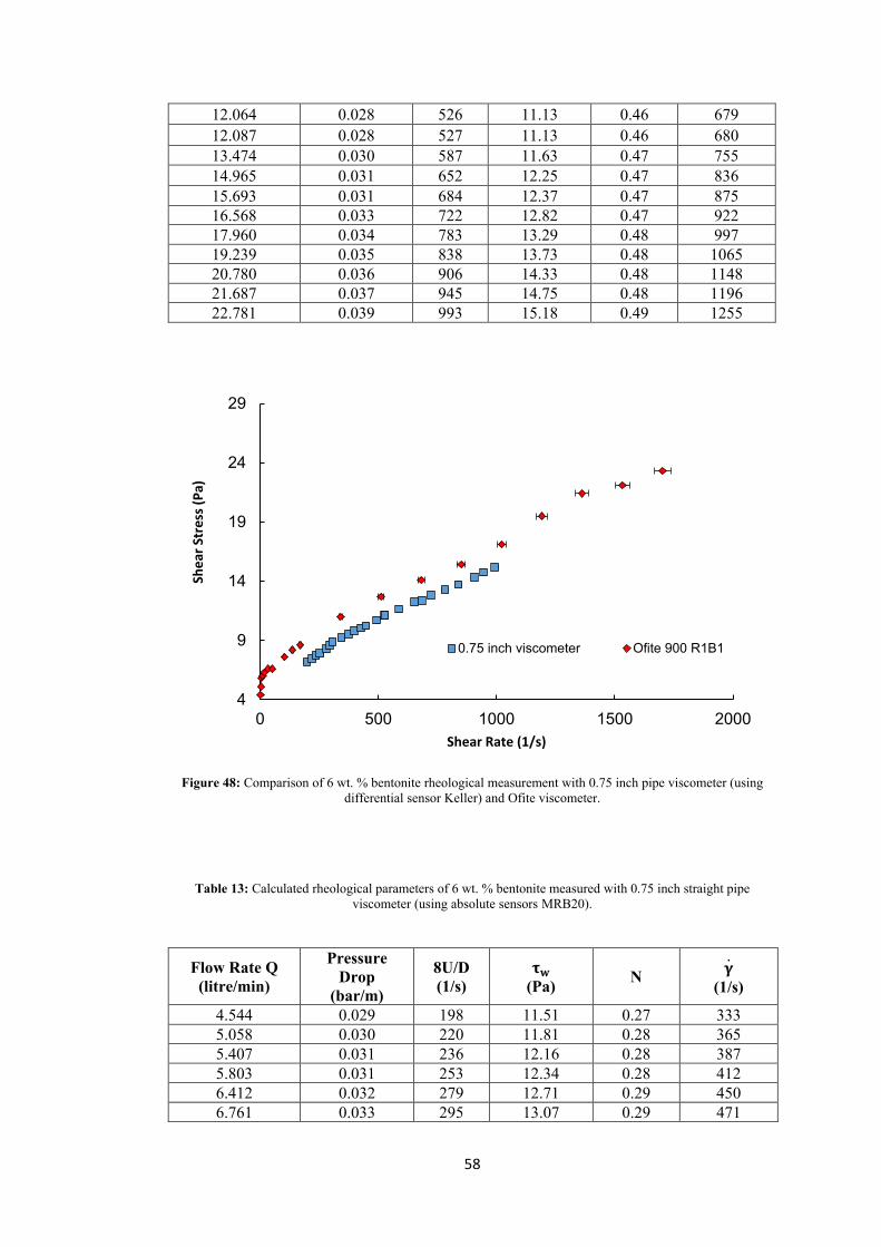
58
Figure 48: Comparison of 6 wt. % bentonite rheological measurement with 0.75 inch pipe viscometer (using
differential sensor Keller) and Ofite viscometer.
Table 13: Calculated rheological parameters of 6 wt. % bentonite measured with 0.75 inch straight pipe viscometer (using absolute sensors MRB20).
4
9
14
19
24
29
0 500 1000 1500 2000
Shea
r Str
ess (
Pa)
Shear Rate (1/s)
0.75 inch viscometer Ofite 900 R1B1
12.064 0.028 526 11.13 0.46 679 12.087 0.028 527 11.13 0.46 680 13.474 0.030 587 11.63 0.47 755 14.965 0.031 652 12.25 0.47 836 15.693 0.031 684 12.37 0.47 875 16.568 0.033 722 12.82 0.47 922 17.960 0.034 783 13.29 0.48 997 19.239 0.035 838 13.73 0.48 1065 20.780 0.036 906 14.33 0.48 1148 21.687 0.037 945 14.75 0.48 1196 22.781 0.039 993 15.18 0.49 1255
Flow Rate Q (litre/min)
Pressure Drop
(bar/m)
8U/D (1/s)
𝛕𝛕𝐰𝐰 (Pa) N 𝛄𝛄 ̇
(1/s)
4.544 0.029 198 11.51 0.27 333 5.058 0.030 220 11.81 0.28 365 5.407 0.031 236 12.16 0.28 387 5.803 0.031 253 12.34 0.28 412 6.412 0.032 279 12.71 0.29 450 6.761 0.033 295 13.07 0.29 471
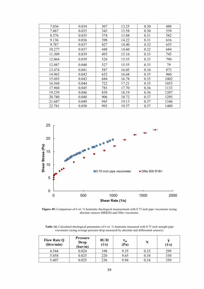
59
Figure 49: Comparison of 6 wt. % bentonite rheological measurement with 0.75 inch pipe viscometer (using
absolute sensors MRB20) and Ofite viscometer.
Table 14: Calculated rheological parameters of 6 wt. % bentonite measured with 0.75 inch straight pipe viscometer (using average pressure drop measured by absolute and differential sensors).
Flow Rate Q (litre/min)
Pressure Drop
(bar/m)
8U/D (1/s)
𝛕𝛕𝐰𝐰 (Pa) N 𝛄𝛄 ̇
(1/s)
4.544 0.024 198 9.35 0.33 299 5.058 0.025 220 9.65 0.34 330 5.407 0.025 236 9.94 0.34 350
0
5
10
15
20
25
0 500 1000 1500 2000
Shea
r Str
ess
(Pa)
Shear Rate (1/s)
0.75 inch pipe viscometer Ofite 900 R1B1
7.036 0.034 307 13.25 0.30 488 7.867 0.035 343 13.58 0.30 539 8.576 0.035 374 13.88 0.31 582 9.136 0.036 398 14.22 0.31 616 9.787 0.037 427 14.40 0.32 655
10.277 0.037 448 14.60 0.32 684 11.309 0.039 493 15.16 0.33 745 12.064 0.039 526 15.55 0.33 790 12.087 0.040 527 15.55 0.33 79 13.474 0.041 587 16.05 0.34 873 14.965 0.042 652 16.68 0.35 960 15.693 0.043 684 16.78 0.35 1002 16.568 0.044 722 17.21 0.35 1053 17.960 0.045 783 17.70 0.36 1133 19.239 0.046 838 18.19 0.36 1207 20.780 0.048 906 18.72 0.37 1295 21.687 0.049 945 19.13 0.37 1346 22.781 0.050 993 19.57 0.37 1409
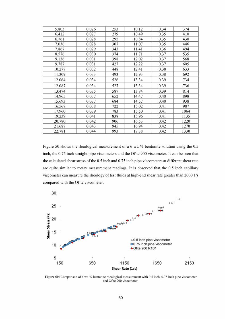
60
5.803 0.026 253 10.12 0.34 374 6.412 0.027 279 10.49 0.35 410 6.761 0.028 295 10.84 0.35 430 7.036 0.028 307 11.07 0.35 446 7.867 0.029 343 11.41 0.36 494 8.576 0.030 374 11.71 0.37 535 9.136 0.031 398 12.02 0.37 568 9.787 0.031 427 12.22 0.37 605
10.277 0.032 448 12.41 0.38 633 11.309 0.033 493 12.93 0.38 692 12.064 0.034 526 13.34 0.39 734 12.087 0.034 527 13.34 0.39 736 13.474 0.035 587 13.84 0.39 814 14.965 0.037 652 14.47 0.40 898 15.693 0.037 684 14.57 0.40 938 16.568 0.038 722 15.02 0.41 987 17.960 0.039 783 15.50 0.41 1064 19.239 0.041 838 15.96 0.41 1135 20.780 0.042 906 16.53 0.42 1220 21.687 0.043 945 16.94 0.42 1270 22.781 0.044 993 17.38 0.42 1330
Figure 50 shows the rheological measurement of a 6 wt. % bentonite solution using the 0.5
inch, the 0.75 inch straight pipe viscometers and the Ofite 900 viscometer. It can be seen that
the calculated shear stress of the 0.5 inch and 0.75 inch pipe viscometers at different shear rate
are quite similar to rotary measurement readings. It is observed that the 0.5 inch capillary
viscometer can measure the rheology of test fluids at high-end shear rate greater than 2000 1/s
compared with the Ofite viscometer.
Figure 50: Comparison of 6 wt. % bentonite rheological measurement with 0.5 inch, 0.75 inch pipe viscometer
and Ofite 900 viscometer.
5
10
15
20
25
30
150 650 1150 1650 2150
Shea
r Str
ess (
Pa)
Shear Rate (1/s)
0.5 inch pipe viscometer0.75 inch pipe viscometerOfite 900 R1B1

61
Figure 51, similarly, shows the rheological measurement of a 6 wt. % bentonite solution to
compare a 1 inch straight pipe viscometer to the Ofite 900. It illustrates that the measurements
between the two viscometers are different This is attributed to small values of pressure drop
within the test section of the 1 inch pipe, which leads to inaccurate measurement of shear stress.
Figure 51: Comparison of 6 wt. % bentonite rheological measurement with 1 inch pipe viscometer and Ofite 900 viscometer.
A hydraulic experiment was conducted to predict the friction loss of bentonite flowing along
the 0.5 inch straight pipe. The rheological data and density of 6 wt. % bentonite were measured
by the Ofite 900 viscometer and mud balance under controlled temperature for the pressure
drop prediction. The full rheology measurement of the test sample is presented in [Figure 52].
The density of test fluid is 1060kg/m3. Three rheological models are chosen for the regression
of 6 wt. % bentonite full measurement including the Bingham Plastic, Power-Law and H-B
models from [Table 2]. The corresponding rheological parameters are calculated and shown
in [Table 15]. Extensive model evaluation from Figure 34 to 36 was conducted to predict the
pressure drop of bentonite flowing along the 0.5 inch straight pipe viscometer, as detailed in
[Table 16]. The experimental flow rates of laminar flow condition began from 4.422 lpm to
15.266 lpm, as shown in the plot of pressure drop versus flow rate, in [Figure 53].
0
5
10
15
20
25
0 500 1000 1500 2000
Shea
r Str
ess (
Pa)
Shear Rate (1/s)
1 inch pipe viscometer Ofite 900 R1B1

62
Figure 52: Full rheological measurement of 6 wt. % bentonite using Ofite 900 viscometer.
Table 15: Rheological constants of 6 wt. % bentonite for 0.5 inch pipe viscometer.
Pipe Viscometer Bingham Plastic Power Law Herschel-Bulkley
0.5 inch τ = 6.16 Pa
μp = 0.0108 Pa K=3.3205
N=0.2303
τ = 4.355 Pa
K=3.3205
N=0.2303
Table 16: Calculation of pressure drop of 6 wt. % bentonite in laminar flow condition measuring with 0.5 inch pipe viscometer.
Flow Rate Q (litre/min)
Measured DP (bar/m)
Predicted DP (bar/m)
Bingham Plastic Power Law Herschel -
Bulkley 4.422 0.052 0.053 0.097 0.059 4.698 0.054 0.054 0.098 0.061 5.279 0.050 0.057 0.101 0.064 5.908 0.056 0.061 0.103 0.067 6.402 0.058 0.063 0.105 0.069 6.635 0.056 0.064 0.106 0.071 7.427 0.060 0.068 0.109 0.074 7.608 0.063 0.069 0.109 0.075 8.256 0.067 0.073 0.112 0.078 8.717 0.068 0.075 0.113 0.080 9.509 0.072 0.079 0.115 0.083
0
5
10
15
20
25
0 500 1000 1500 2000
Shea
r Str
ess (
Pa)
Shear Rate (1/s)
6% Bentonite Ofite 900 Viscometer measurement

63
10.049 0.075 0.082 0.117 0.085 10.921 0.079 0.087 0.119 0.088 11.374 0.081 0.089 0.120 0.090 12.103 0.084 0.093 0.122 0.093 13.073 0.090 0.098 0.124 0.096 14.369 0.096 0.104 0.127 0.100 15.266 0.102 0.109 0.128 0.103
Figure 53: Pressure loss predictions of three different rheological models.
It can be seen from Figure 53 that the Power Law model prediction produces a poor estimation
of pressure drop at different flow rates. The friction loss prediction of 6 wt. % bentonite using
the Bingham plastic and Herschel-Bulkley models are considerably closer to the measured
pressure drop. It should be noted that the conventional approach of pressure drop prediction is
based on the rheological constants. The particular choice of the rheological constants of
rheological models when data fitting, could affect the determination of friction loss of the test
fluid flowing in hydraulic circuits. It is noteworthy that rheological parameters at different
ranges of shear rate also result in different rheological constants. To increase the accuracy of
pressure drop prediction, the rheological model parameters are required to be determined over
the shear rate range in which the pressure drop is determined.
It is also possible to use pipe viscometer data to calculate the pressure drop directly. This can
be performed using the relationship between shear stress and shear rate, as given in equations
(2.5) and (2.7). For a given flow rate, the nominal shear rate can be determined, and
0.04
0.05
0.06
0.07
0.08
0.09
0.10
0.11
0.12
0.13
0.14
4 6 8 10 12 14 16
Pres
sure
dro
p (b
ar/m
)
Flow rate (lpm)
Measured pressure dropBingham plastic predictionPower Law predictionH-B prediction
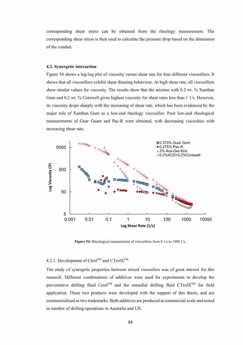
64
corresponding shear stress can be obtained from the rheology measurement. The
corresponding shear stress is then used to calculate the pressure drop based on the dimension
of the conduit.
4.2. Synergetic interaction
Figure 54 shows a log-log plot of viscosity versus shear rate for four different viscosifiers. It
shows that all viscosifiers exhibit shear thinning behaviour. At high shear rate, all viscosifiers
show similar values for viscosity. The results show that the mixture with 0.2 wt. % Xanthan
Gum and 0.2 wt. % Corewell gives highest viscosity for shear rates less than 1 1/s. However,
its viscosity drops sharply with the increasing of shear rate, which has been evidenced by the
major role of Xanthan Gum as a low-end rheology viscosifier. Poor low-end rheological
measurements of Guar Guam and Pac-R were obtained, with decreasing viscosities with
increasing shear rate.
Figure 54: Rheological measurement of viscosifiers from 0 1/s to 1900 1/s.
4.2.1. Development of CtrolTM and CTrolXTM
The study of synergetic properties between mixed viscosifers was of great interest for this
research. Different combinations of additives were used for experiments to develop the
preventative drilling fluid CtrolTM and the remedial drilling fluid CTrolXTM for field
application. These two products were developed with the support of this thesis, and are
commercialised as two trademarks. Both additives are produced at commercial scale and tested
in number of drilling operations in Australia and US.
5
50
500
5000
0.001 0.01 0.1 1 10 100 1000 10000
Log
Visc
osity
CP)
Log Shear Rate (1/s)
0.375% Guar Gum0.275% Pac-R3% Aus-Gel-Xtra0.2%XCD+0.2%Corewell
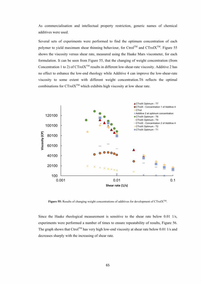
65
As commercialisation and intellectual property restriction, generic names of chemical
additives were used.
Several sets of experiments were performed to find the optimum concentration of each
polymer to yield maximum shear thinning behaviour, for CtrolTM and CTrolXTM. Figure 55
shows the viscosity versus shear rate, measured using the Haake Mars viscometer, for each
formulation. It can be seen from Figure 55, that the changing of weight concentration (from
Concentration 1 to 2) of CTrolXTM results in different low-shear-rate viscosity. Additive 2 has
no effect to enhance the low-end rheology while Additive 4 can improve the low-shear-rate
viscosity to some extent with different weight concentration.T6 reflects the optimal
combinations for CTrolXTM which exhibits high viscosity at low shear rate.
Figure 55: Results of changing weight concentrations of additives for development of CTrolXTM.
Since the Haake rheological measurement is sensitive to the shear rate below 0.01 1/s,
experiments were performed a number of times to ensure repeatability of results, Figure 56.
The graph shows that CtrolTM has very high low-end viscosity at shear rate below 0.01 1/s and
decreases sharply with the increasing of shear rate.
100
20100
40100
60100
80100
100100
120100
0.001 0.01 0.1
Visc
osity
(CP)
Shear rate (1/s)
CTrolX Optimum - T7CTrolX - Concentration 1 of Additive 4CTrolAdditive 2 at optimum concentrationCTrolX Optimum - T6CTrolX Optimum - T4CTrolX - Concentration 2 of Additive 4CTrolX Optimum - T2CTrolX Optimum - T1

66
Figure 56: Repeatability of CtrolTM measurements.
4.2.2. Field application of CtrolTM and CTrolXTM
These experiments are performed by Drilling Mechanics Group researchers for benchmarking
CtrolTM with other commercial fluids and also using CtrolTM in the field for two Coiled Tubing
drilling operations using RoXplorer drilling rig in Victoria Australia [Figure 57].
In the coiled tube drilling trial, the RoXplorer was a revolutionary drill rig for mineral
exploration that utilises continuous steel coil. The downhole mud motor systems of RoXplorer,
made of a positive displacement motor and a downhole hammer, were connected to 500 meters
of coiled tube. The downhole motors received hydraulic energy from the drilling mud to
deliver rotary and reciprocating movements to the percussive bit. This coiled tubing drilling
allowed for continuous drilling and pumping and increased the rate of penetration, making
drilling faster, cheaper and safer than conventional drilling.
Figure 57: Coiled tube drilling system, RoXplorer, used in the drilling trials in Australia - courtesy DET CRC.

67
The benchmark experiments in the field were performed to compare the efficiency of CtrolTM
and CtrolXTM with two commercial drilling fluid systems. After each experiment, water was
circulated to return fluid loss level to the initial value before testing the new drilling fluid.
Figure 58 shows the fluid loss variation with flow rate, for CtrolTM, CtrolXTM and two
commercial polymers. Figure 59 shows flow return after CtrolTM invasion into unconsolidated
formations. It can be seen from these figures that CtrolTM and CtrolXTM established significant
flow return comparing with two other commercial drilling fluid systems.
Figure 58: The benchmark of CtrolTM and CTrolXTM in the field (Mostofi and Samani 2017).
Figure 59: Establishing return after CtrolTM invasion into unconsolidated formations. The data collected from the RoXplorer field trial in Victoria. (Mostofi and Samani 2018).

68
4.3. Particle effect on rheology
In the following section, the effects of solids concentration and size on the viscosity of
suspensions are presented. The experiments were designed to investigate the effect of solid
particles on polymer viscosity at different shear rates and also the change in thixotropic
property.
As previous literature suggested that the cuttings settling velocity in suspension decreases
significantly with increasing of the particle volume concentration whilst increasing with
increase in particle size [45], thus, a Haake step-wise experiment was designed to verify this
using the Haake viscomter with a suspension of 0.5 wt. % Xanthan Gum with 0.3 vol. % silica
sand, at a size range of 250-300 micron. The shear rate was ramped up from zero shear rate to
1900 1/s and then ramped down from 1900 1/s to zero shear rate. Figure 60 shows the plot of
shear rate versus time for ramp-up and ramp-down. The measured viscosity at shear rates of
100 1/s and 1000 1/s for ramp-up and ramp-down are denoted on the Figure 60 as points A, D
and points B, C respectively. It can been seen that the difference in viscosity at each shear rate,
between ramp-up and ramp-down are minimum. This suggests no significant effect of
sedimentation on the experiment of viscosity.
Figure 60: Haake step-wise measurement of suspension with 0.3 vol. % sand at size range of 250-300 micron.
The effect of solid volume concentration on the rheology of suspensions are shown in Figure
61 to Figure 64. Here, suspensions of silica sand of different size distributions (106-200,200-
250 and 250-300 μm) and volume concentrations (0.3-3.0%), and 38-75 μm Calcium
Carbonate particles with different volume concentrations (0.3-3.0%) were used to measure
viscosity versus shear rate, using the Haake Mars Z20DIN viscometer and the blank fluid
0.5wt. % Xanthan Gum.
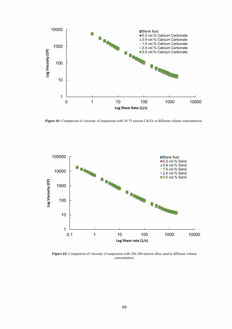
69
Figure 61: Comparison of viscosity of suspension with 38-75 micron CaCO3 at different volume concentration.
Figure 62: Comparison of viscosity of suspension with 106-200 micron silica sand at different volume
concentration.
1
10
100
1000
10000
0 1 10 100 1000 10000
Log
Visc
osity
(CP)
Log Shear Rate (1/s)
Blank fluid0.3 vol.% Calcium Carbonate0.9 vol.% Calcium Carbonate1.5 vol.% Calcium Carbonate2.4 vol.% Calcium Carbonate3.0 vol.% Calcium Carbonate
1
10
100
1000
10000
100000
0.1 1 10 100 1000 10000
Log
Visc
osity
(CP)
Log Shear rate (1/s)
Blank fluid0.3 vol.% Sand0.9 vol.% Sand1.5 vol.% Sand2.4 vol.% Sand3.0 vol.% Sand

70
Figure 63: Comparison of viscosity of suspension with 200-250 micron silica sand at different volume
concentration.
Figure 64: Comparison of viscosity of suspension with 250-300 micron silica sand at different volume
concentration.
1
10
100
1000
10000
0.1 1 10 100 1000 10000
Log
Visc
osity
(CP)
Log Shear rate (1/s)
Blank fluid0.3 vol.% Sand0.9 vol.% Sand1.5 vol.% Sand2.4 vol.% Sand3.0 vol.% Sand
1
10
100
1000
10000
0.1 1 10 100 1000 10000
Log
Visc
osity
(CP)
Log Shear Rate (1/s)
Blank fluid0.3 vol.% Sand0.9 vol.% Sand1.5 vol.% Sand

71
The data in Figure 61 - Figure 64 suggests that there is a minimum change in the viscosity of
suspensions solutions as compared with the blank solution, for the suspensions used in the
experiments. To better characterise the effect of solid particles on the fluid rheology, the
relative viscosity ηr is obtained for each suspension solution, defined as:
ηr =ηsηb
(4.3)
where ηs is the suspension viscosity and ηb is the blank fluid viscosity, which is the viscosity
of the suspending fluid without solid particles. The effect of solid particles on the fluid can be
reflected in the magnitude of relative viscosity.
Figure 65: Relative viscosity of suspensions with 3.0 vol. % particles at shear rate from 0 to 1900 1/s.
Figure 65 shows that the relative viscosity seems to be smaller at lower shear rates, and
increases gradually with shear rate. As shown in the graph, the relative viscosity of Calcium
Carbonate solution at low shear rate as low as 1.01, and increases gradually reaching a
maximal relative viscosity of 1.3 at approximately 700 1/s shear rate. A similar trend can be
observed for the suspension with silica sand. One possible explanation for this trend is that
particles can form aggregates at low shear condition, and therefore shear will produce less
interaction between aggregated cuttings. However, the established network breaks at medium
or high shear rates (greater than 700 1/s), and the interaction of particles increases rapidly, and
as a result the suspension viscosity increases.
0.95
1.00
1.05
1.10
1.15
1.20
1.25
1.30
0 1 10 100 1000 10000
Rela
tive
visc
osiy
Log Shear rate (1/s)
Calcium Carbonate106-200 micron Sand
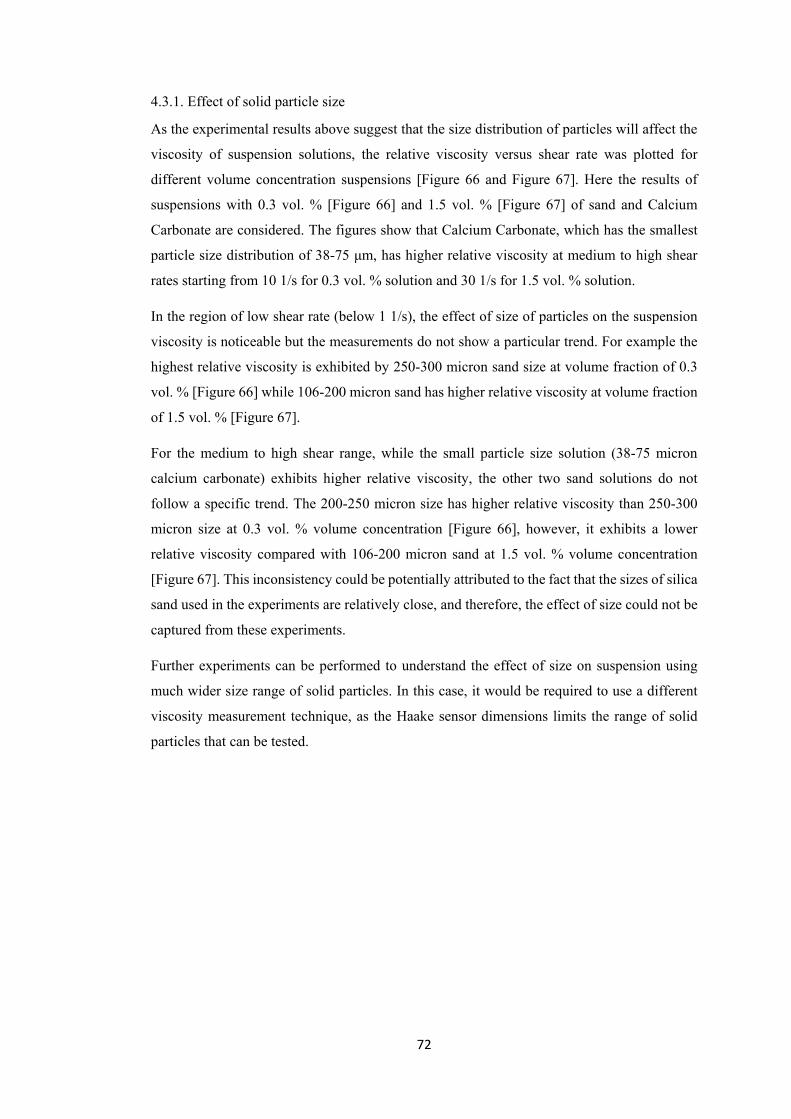
72
4.3.1. Effect of solid particle size
As the experimental results above suggest that the size distribution of particles will affect the
viscosity of suspension solutions, the relative viscosity versus shear rate was plotted for
different volume concentration suspensions [Figure 66 and Figure 67]. Here the results of
suspensions with 0.3 vol. % [Figure 66] and 1.5 vol. % [Figure 67] of sand and Calcium
Carbonate are considered. The figures show that Calcium Carbonate, which has the smallest
particle size distribution of 38-75 μm, has higher relative viscosity at medium to high shear
rates starting from 10 1/s for 0.3 vol. % solution and 30 1/s for 1.5 vol. % solution.
In the region of low shear rate (below 1 1/s), the effect of size of particles on the suspension
viscosity is noticeable but the measurements do not show a particular trend. For example the
highest relative viscosity is exhibited by 250-300 micron sand size at volume fraction of 0.3
vol. % [Figure 66] while 106-200 micron sand has higher relative viscosity at volume fraction
of 1.5 vol. % [Figure 67].
For the medium to high shear range, while the small particle size solution (38-75 micron
calcium carbonate) exhibits higher relative viscosity, the other two sand solutions do not
follow a specific trend. The 200-250 micron size has higher relative viscosity than 250-300
micron size at 0.3 vol. % volume concentration [Figure 66], however, it exhibits a lower
relative viscosity compared with 106-200 micron sand at 1.5 vol. % volume concentration
[Figure 67]. This inconsistency could be potentially attributed to the fact that the sizes of silica
sand used in the experiments are relatively close, and therefore, the effect of size could not be
captured from these experiments.
Further experiments can be performed to understand the effect of size on suspension using
much wider size range of solid particles. In this case, it would be required to use a different
viscosity measurement technique, as the Haake sensor dimensions limits the range of solid
particles that can be tested.
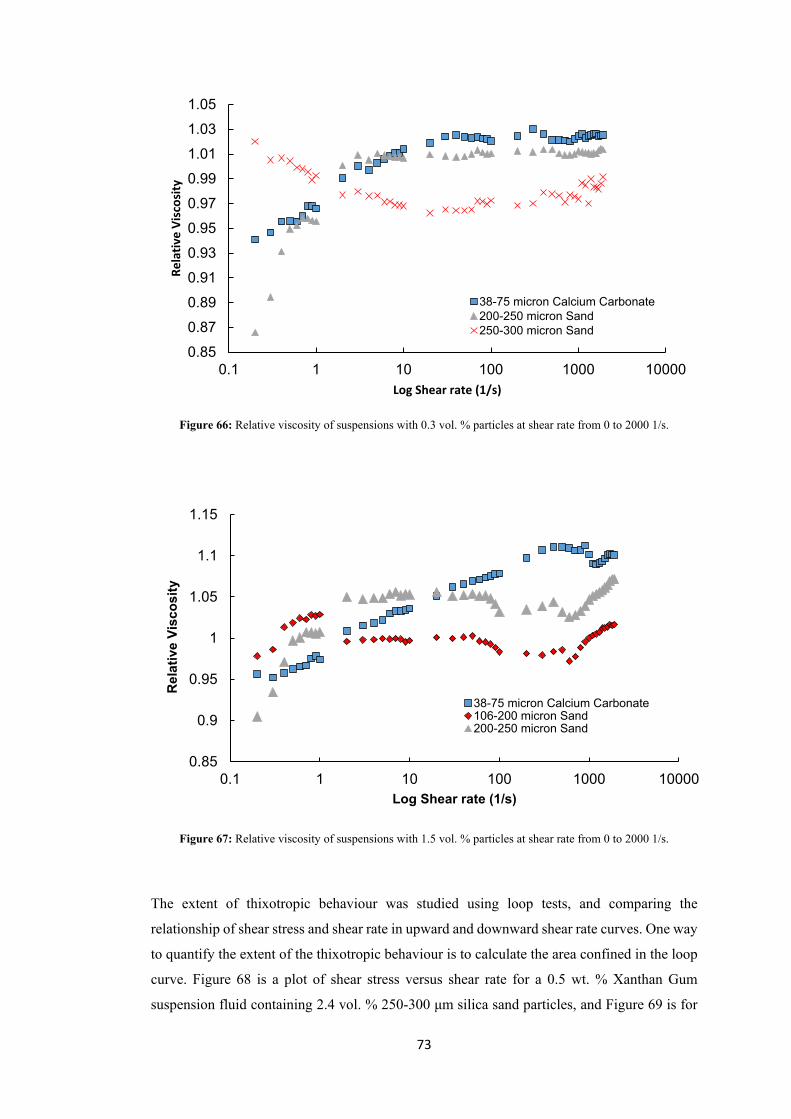
73
Figure 66: Relative viscosity of suspensions with 0.3 vol. % particles at shear rate from 0 to 2000 1/s.
Figure 67: Relative viscosity of suspensions with 1.5 vol. % particles at shear rate from 0 to 2000 1/s.
The extent of thixotropic behaviour was studied using loop tests, and comparing the
relationship of shear stress and shear rate in upward and downward shear rate curves. One way
to quantify the extent of the thixotropic behaviour is to calculate the area confined in the loop
curve. Figure 68 is a plot of shear stress versus shear rate for a 0.5 wt. % Xanthan Gum
suspension fluid containing 2.4 vol. % 250-300 μm silica sand particles, and Figure 69 is for
0.85
0.87
0.89
0.91
0.93
0.95
0.97
0.99
1.01
1.03
1.05
0.1 1 10 100 1000 10000
Rela
tive
Visc
osity
Log Shear rate (1/s)
38-75 micron Calcium Carbonate200-250 micron Sand250-300 micron Sand
0.85
0.9
0.95
1
1.05
1.1
1.15
0.1 1 10 100 1000 10000
Rel
ativ
e Vi
scos
ity
Log Shear rate (1/s)
38-75 micron Calcium Carbonate106-200 micron Sand200-250 micron Sand
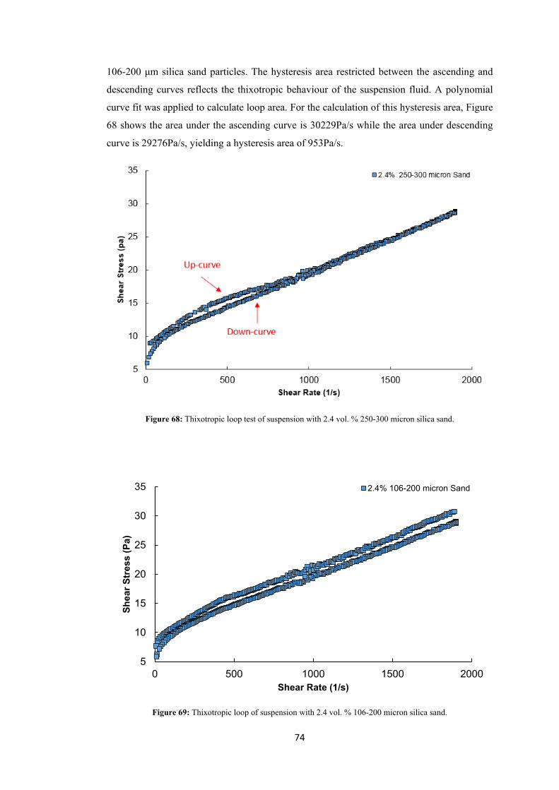
74
106-200 μm silica sand particles. The hysteresis area restricted between the ascending and
descending curves reflects the thixotropic behaviour of the suspension fluid. A polynomial
curve fit was applied to calculate loop area. For the calculation of this hysteresis area, Figure
68 shows the area under the ascending curve is 30229Pa/s while the area under descending
curve is 29276Pa/s, yielding a hysteresis area of 953Pa/s.
Figure 68: Thixotropic loop test of suspension with 2.4 vol. % 250-300 micron silica sand.
Figure 69: Thixotropic loop of suspension with 2.4 vol. % 106-200 micron silica sand.
5
10
15
20
25
30
35
0 500 1000 1500 2000
Shea
r Str
ess
(Pa)
Shear Rate (1/s)
2.4% 106-200 micron Sand

75
The calculated area of loop tests with 2.4 vol. % of different particle sizes are shown in
Table 17.
Table 17: Thixotropic loop tests of 2.4 vol. % of CaCO3 and silica sand suspensions with different particles sizes.
Particle Particle Size
(microns)
Solids Concentration
(vol. %) Hysteresis Area Value
Calcium Carbonate 38-75
2.4
14
Silica Sand
106-200 2666
200-250 367
250-300 953
Based on Table 17, and the loop area shown in Figure 68 and Figure 69, it can be concluded
that the presence of cutting increases thixotropic behaviour, however, the extent is not
correlated with the size of particles. It is worth mentioning that more consistent results could
be obtained by repeating the experiments using different measurement gap-times.
4.3.2. Effect of solid particle concentration
In order to better demonstrate the effect of solid concentrations, the viscosity of suspensions
with Calcium Carbonate and silica sand are considered. The plot of relative viscosity at
different concentrations of particles is plotted for shear rates of 0 to 1 1/s and 100 to 1900
1/s .The relation between solid volume concentration and relative viscosity is shown in Figure
70 to Figure 73. The experimental data in the figure suggests that the relative viscosity
increases with increase in volume concentration of solid particles.
Figure 70 to Figure 73 show the relation between the volume concentrations of Calcium
Carbonate/fine sand particles and the relative viscosity of suspensions from low-end to high
end rheology. For suspensions with the same particle size, the relative viscosity of suspensions
increases with increasing particle volume concentrations at the same shear rate. This trend is
more obvious for particles with volume concentrations greater than 2.4 vol. % at low-end
rheology (shear rate less than 1 1/s). One possible explanation is that the increase in particle
concentration enhances particle-particle interactions. The inner particle force of fine cuttings
dominates at low shear rates which giving a large increase in viscosity. Furthermore, from
medium to high shear rate starting from 100 1/s, the gradient of curve is almost constant,
indicating that the relative viscosities of different calcium carbonate suspensions have no
significant change with the increasing shear rates in this range.
76
Figure 70: Relative viscosity of CaCO3 suspensions with different volume concentration at shear rate from 0 to 1
1/s.
Figure 71: Relative viscosity of CaCO3 suspensions with different volume concentration at shear rate from 100 to 1900 1/s.
0.93
0.94
0.95
0.96
0.97
0.98
0.99
1.00
1.01
1.02
1.03
0.0 0.2 0.4 0.6 0.8 1.0
Rela
tive
Visc
osity
Shear Rate(1/s)
0.3 vol.% 0.9 vol.% 1.5 vol.%2.4 vol.% 3.0 vol.%
1.00
1.05
1.10
1.15
1.20
1.25
1.30
1.35
100 600 1100 1600 2100
Rela
tive
Visc
osity
Shear Rate(1/s)
0.3 vol.% 0.9 vol.% 1.5 vol.%2.4 vol.% 3.0 vol.%

77
Figure 72: Relative viscosity of 200-250 micron sand suspensions with different volume concentration at shear
rate from 0 to 1 1/s.
Figure 73: Relative viscosity of 200-250 micron sand suspensions with different volume concentration at shear rate from 100 to 1900 1/s.
0.80
0.85
0.90
0.95
1.00
1.05
1.10
0 0.2 0.4 0.6 0.8 1
Rela
tive
Visc
osity
Shear Rate(1/s)
0.3 vol.% 0.9 vol.% 1.5 vol.%2.4 vol.% 3.0 vol.%
1.00
1.02
1.04
1.06
1.08
1.10
1.12
1.14
100 600 1100 1600 2100
Rela
tive
Visc
osity
Shear Rate(1/s)
0.3 vol.% 0.9 vol.% 1.5 vol.%2.4 vol.% 3.0 vol.%

78
In Figure 74, the variation of relative viscosity with different concentration at specific shear
rate is illustrated. The data suggests that the relative viscosity increases with increasing volume
concentration of solid particles.
Figure 74: Relative viscosity of 38-75 micron CaCO3 with different volume concentration at specific shear rate.
To investigate the effect of concentration of solid particles on the extent of the thixotropic
behaviour, the loop tests of suspensions with Calcium Carbonate and silica sand of dispersed
and agglomerative conditions were performed. [Figure 75] and [Figure 76] show plots of shear
stress versus shear rate for the loop tests performed on 0.9 vol.% and 1.5 vol.% respectively.
Figure 75: Thixotropic loop of suspension with 0.9 vol. % 106-200 micron silica sand.
0.9
0.95
1
1.05
1.1
1.15
1.2
1.25
0.0 0.5 1.0 1.5 2.0 2.5 3.0
Rela
tive
Visc
osity
Paticle Volume Concentration (%)
Shear Rate at 0.2 1/sShear Rate at 1 1/sShear Rate at 10 1/sShear Rate at 100 1/sShear Rate at 1000 1/sShear Rate at 1900 1/s
5
10
15
20
25
30
0 500 1000 1500 2000
Shea
r Str
ess (
Pa)
Shear Rate (1/s)
0.9% 106-200 micron Sand
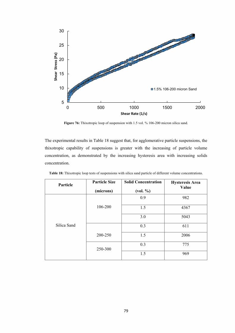
79
Figure 76: Thixotropic loop of suspension with 1.5 vol. % 106-200 micron silica sand.
The experimental results in Table 18 suggest that, for agglomerative particle suspensions, the
thixotropic capability of suspensions is greater with the increasing of particle volume
concentration, as demonstrated by the increasing hysteresis area with increasing solids
concentration.
Table 18: Thixotropic loop tests of suspensions with silica sand particle of different volume concentrations.
Particle Particle Size
(microns)
Solid Concentration
(vol. %)
Hysteresis Area Value
Silica Sand
106-200
0.9 982
1.5 4367
3.0 5043
200-250
0.3 611
1.5 2006
250-300 0.3 775
1.5 969
5
10
15
20
25
30
0 500 1000 1500 2000
Shea
r St
ress
(Pa)
Shear Rate (1/s)
1.5% 106-200 micron Sand

80
It can be concluded from the experiment results that the volume fraction of particles in
suspension significantly affects the viscosity of mono-dispersed suspensions with fine
particles. The effect of particle size is minimal during medium and high shear rate regions, for
the fluids under investigation. Furthermore, the suspension viscosity also depends on the
imposed range of shear rate.
It is noteworthy that the impact of solid suspensions on the suspension rheology can be also
affected by the viscosity of suspending liquid. For example, the extent of the effect could be
potentially different if the suspending fluid has a different viscosity. For practical applications,
lower viscosities are more relevant for drilling operation, however, the settlement of the
particles during drilling operation is an issue that requires further investigation, and therefore,
different measurement techniques should be incorporated. In future research, the pipe
viscometer will be used to investigate the rheology of suspensions.
81
Chapter 5. Conclusion This thesis was focused on the rheology of drilling fluids. The work began with a review of
different measurement techniques, followed by benchmarking the fluid rheology obtained
from different viscosifiers (drilling fluid additives). The interaction between different
polymers was studied experimentally, which led to the development of two drilling fluid
systems, CtrolTM and CTrolXTM, for preventative and remedial drilling fluid loss respectively.
Finally, the effect of drill cuttings on the fluid rheology studied at a wide range of shear rates.
A summary of key findings are presented below.
5.1. Effective methods of drilling fluid viscosity measurement
There are different measurement techniques developed and standardised within drilling
engineering to measure and represent the viscosity of drilling fluid. These methods are
reported as part of API standards, and are extensively used within the drilling industry as best
practices to design, measure and monitor the drilling fluid in the lab and in the field. These
methods are compared and benchmarked with other measurement techniques, which are more
commonly used in other engineering disciplines.
Different measurement techniques were compared in this thesis. This comparison entailed
measurement techniques using the Marsh Funnel (flow through constriction), different rotary
viscosity measurement equipment (different tools and sensors), and pipe viscometer
(capillary). The results showed that pipe viscometer (different pipe dimensions) and different
rotary viscometers (Haake and Ofite with five different sensor arrangements) have agreement
in terms of viscosity measurements at measured shear rates. However, the measurement of
fluid viscosity using the Marsh Funnel demonstrated that is not a reliable tool to quantify fluid
viscosity even at qualitative level – two fluids with the same Marsh Funnel viscosity exhibited
very different fluid rheology measured using rotary viscometers.
The thesis also reviewed the effectiveness of industry practice of measuring and quantifying
fluid viscosity at only two shear rates of 510 1/s and 1020 1/s. The results of benchmark
experiments obtained from solutions made using common drilling fluid polymers with similar
measurements at high shear rate (1020 1/s), showed that there are significant difference in
fluid rheology: while the high-end rheology of these solutions were almost the same, the low-
end rheology at low shear rates were up to two orders of magnitudes different. The benchmark
results therefore suggest that the response/behaviour of the fluid in processes depending on
low shear rate (e.g. fluid loss control and sedimentation of cuttings within tanks) will be
significantly different for these fluids, while the conventional fluid viscosity measurements
considers these fluids as comparable solutions.
82
5.2. CtrolTM and CTrolXTM drilling fluids
This research work facilitated the development of two drilling fluid systems for fluid loss
control, namely CtrolTM and CTrolXTM. Particularly, the body of experimental work related to
characterising the low-end rheology of different polymer combinations were performed as part
of this thesis. As a part of the research, this thesis also provided laboratory support to
researchers on site (Dr Masood Mostofi and Frank Samani) during the implementation and
field testing of these products. Both products are registered and patented under trademark
names of CtrolTM and CTrolXTM.
CtrolTM is a preventative drilling fluid, which is used under normal drilling operation. The
fluid is designed on the basis of rheological synergies between different natural and synthetic
polymers, which can deliver extensive shear thinning property. CtrolTM exhibits small
viscosities at high shear rates, providing effective hole cleaning, drag deduction and sample
(cutting) delivery to surface (with minimum level of cutting spreading). At low shear rates,
CtrolTM has significantly higher viscosity, which makes the drilling fluid an effective solution
for fluid loss control in unconsolidated grounds and also natural fractures with small apertures.
CTrolXTM is a remedial drilling fluid, which is deployed after drilling natural fractured
formations or after inducing hydraulic fractures to control the fluid loss. CTrolXTM is
injected/circulated when the drilling process is on hold. In this thesis, the low-end rheology of
different polymer and bentonite combinations were tested to derive a recipe with maximum
viscosities at low shear rates (at the range of 0.001-0.1 1/s).
5.3. Effect of fine particles on mono-dispersed suspension rheology
In the final part of this research, the effect of solid fine particles on the polymer rheology was
investigated. The experimental conditions in terms of solid size and concentration were
selected to represent drilling conditions in the field.
The test protocol was developed to minimise any possibility of cuttings settlement during the
experiments. The experiments were performed at low to high shear rates, ranging from 0 1/s
to 1900 1/s. A suspending fluid with high viscosity was used to suspend the cuttings and
minimise the settlement of cuttings during the experiments. The results were interpreted based
on relative viscosity at each shear rate derived from the ratio of suspension fluid viscosity over
the suspending fluid viscosity. The thixotropic property of suspension was measured using a
profile of loop test.
The results showed that shear rate and cutting concentration are two key factors affecting
relative viscosity, and the suspension viscosity is not much affected by the sizes tested in this
research. The effect of cuttings on suspension viscosity was minimum at low shear rates, while

83
the relative viscosity increases continuous with shear rate. Figure 77 illustrates a conceptual
variation of relative viscosity with particle concentration and shear rate. The results confirm
that the relative viscosity is controlled by the concentration of solid particles, and the effect is
higher at higher shear rates.
The thixotropic behaviour of fluids is affected by the presence of cuttings. Even at high
polymer concentration, the suspending fluid exhibited a minimum thixotropic behaviour
measured from hysteresis in the loop experiments. The suspension fluids showed a thixotropic
behaviour, where the area between the ramp up and ramp down of shear rate increases with
cutting concentration. The data also shows that the extent of thixotropic behaviour is not
correlated with the size of particles. These trends are conceptually demonstrated in Figure 78.
Figure 77: (a) variation of relative viscosity with particle concentration, (b) variation of relative viscosity with
shear rate.
Figure 78: Variation of thixotropic loop area with particle concentration.
84
5.4. Recommendations for future work
There are areas that we believe further work can be performed which are not covered here due
to the current limitation in available equipment, time and in expanding the focus of this work.
The mechanisms of interactions between polymers can be further studied. In this work, a pure
experimental and trial and error approach was implemented to derive the optimum
composition of CtrolTM and CTrolXTM. The work benefited from literature specifying possible
combinations and mechanisms that can result in the synergies between different polymers,
however, the mixed solutions were only quantified in terms of resultant viscosity. The
limitations were mainly due to lack of equipment and also possible complex interactions of
the polymer mixture. Indeed, further work can be performed in future research to better
understand the variation of the interaction of the polymer systems.
The effect of cuttings on drilling fluid rheology can be further studied at a larger range of
cutting size, lower viscosity of suspending solution and under dynamic conditions of the
wellbore. Due to equipment limitations (dimensions of the Haake concentric sensor), the range
of cutting size was limited, which can be in part the reason that a particular trend related to the
effect of cuttings on the suspension relative viscosity was not observed. Furthermore,
extremely high viscosity was used for the suspending fluid to ensure that the particles would
not settle during the experiment. Indeed, it is possible that more pronounced effects related to
the solid particles could be observed if a thinner suspending fluid would have been used. These
experiments can be performed in future using a pipe viscometer, in which the dynamic
condition of the pipe in vertical arrangement will be sufficient to suspend and transport the
cuttings. The other benefit of conducting the experiments using the pipe viscometer is that the
measurements will be under the same dynamic conditions of the wellbore where the drilling
fluid transports the cuttings to surface. As part of this research, a pipe viscometer was
developed in the laboratories; however, the complementary experiments to evaluate the effect
of cuttings using a pipe viscometer, under thermal and pressure control were not performed
due to time constrains, and planning is underway to conduct these experiments as part of
doctoral studies after completion of this research work.
85
References [1] Bourgoyne Jr, A.T., et al., Applied drilling engineering. Volume 2. 1986.
[2] Bloys, B., et al., Designing and managing drilling fluid. Oilfield Review, 1994. 6(2): p.
33- 43.
[3] Pitt, M., The Marsh funnel and drilling fluid viscosity: a new equation for field use. SPE
Drilling & Completion, 2000. 15(01): p. 3-6.
[4] Walker, T.O., Additive for reducing fluid loss or filtration rate for aqueous drilling fluid
containing both high salinity and high soluble calcium. 1976, Google Patents.
[5] Fontana, P., L. Watkins, and P. Aronstam, Drilling system and method for controlling
equivalent circulating density during drilling of wellbores. 2007, Google Patents.
[6] Chen, G., et al., A study of wellbore stability in shales including poroelastic, chemical,
and thermal effects. Journal of Petroleum Science and Engineering, 2003. 38(3-4): p.
167-176.
[7] Barnes, H.A., J.F. Hutton, and K. Walters, An introduction to rheology. 1989: Elsevier.
[8] Barnes, H.A., Thixotropy—a review. Journal of Non-Newtonian fluid mechanics, 1997.
70(1-2): p. 1-33.
[9] Chhabra, R.P. and J.F. Richardson, Non-Newtonian flow and applied rheology:
engineering applications. 2011: Butterworth-Heinemann.
[10] Hemphill, T., W. Campos, and A. Pilehvari, Yield-power law model more accurately
predicts mud rheology. Oil and Gas Journal;(United States), 1993. 91(34).
[11] Huang, X. and M.H. Garcia, A Herschel–Bulkley model for mud flow down a slope.
Journal of fluid mechanics, 1998. 374: p. 305-333.
[12] Garakani, A.K., et al., Comparison between different models for rheological
characterization of activated sludge. Iranian journal of environmental health science &
engineering, 2011. 8(3): p. 255.
[13] Roussel, N. and R. Le Roy, The Marsh cone: a test or a rheological apparatus? Cement
and concrete research, 2005. 35(5): p. 823-830.
[14] Kumar, A. and R.K. Gupta, Fundamentals of polymer engineering, revised and expanded.
2003: CRC Press.
[15] API, R., 13D.(2010). Standard procedure for rheology and hydraulics of oil-well fluids.
Recommended practice Sixed Edition, May. American Petroleum Institute.
[16] Accessory, A.B.V., Brookfield Engineering Laboratories. Inc., Stoughton, Massachusetts,
date unknown.
[17] Kang, Y.J., S.Y. Yoon, and S. Yang. Viscosity measurement using hydrodynamic
divergencing chamber and digital counting in microfluidic channels. in 2010 IEEE 23rd
International Conference on Micro Electro Mechanical Systems (MEMS). 2010. IEEE.
[18] Munson, B.R., et al., Fundamentals of fluid mechanics. 2014: John Wiley & Sons.
86
[19] Collins, M. and W. Schowalter, Behavior of non‐Newtonian fluids in the entry region of
a pipe. AIChE journal, 1963. 9(6): p. 804-809.
[20] Barker, B. Massecuite consistency measurement using a pipeline viscometer. in Proc S
Afr Sug Technol Ass. 2008.
[21] Vajargah, A.K. and E. van Oort, Determination of drilling fluid rheology under downhole
conditions by using real-time distributed pressure data. Journal of Natural Gas Science
and Engineering, 2015. 24: p. 400-411.
[22] Rommetveit, R. and K. Bjorkevoll. Temperature and pressure effects on drilling fluid
rheology and ECD in very deep wells. in SPE/IADC Middle East Drilling Technology
Conference. 1997. Society of Petroleum Engineers.
[23] Ford, J., et al. Experimental investigation of drilled cuttings transport in inclined
boreholes. in SPE Annual Technical Conference and Exhibition. 1990. Society of
Petroleum Engineers.
[24] Shauly, A., A. Wachs, and A. Nir, Shear-induced particle migration in a polydisperse
concentrated suspension. Journal of Rheology, 1998. 42(6): p. 1329-1348.
[25] Fadairo, A., D. Orodu, and O. Falode. Investigating the carrying capacity and the effect
of drilling cutting on rheological properties of jatropha oil based mud. in SPE Nigeria
annual international conference and exhibition. 2013. Society of Petroleum Engineers.
[26] Mahto, V. and V. Sharma, Rheological study of a water based oil well drilling fluid.
Journal of Petroleum Science and Engineering, 2004. 45(1-2): p. 123-128.
[27] Bergström, L., Shear thinning and shear thickening of concentrated ceramic suspensions.
Colloids and Surfaces A: Physicochemical and Engineering Aspects, 1998. 133(1-2): p.
151-155.
[28] Coussot, P., Mudflow rheology and dynamics. 2017: Routledge.
[29] Peker, S.M. and S.S. Helvaci, Solid-liquid two phase flow. 2011: Elsevier.
[30] Watanabe, Y., A. Kawamoto, and K. Matsuda, Particle size distributions in functionally
graded materials fabricated by the centrifugal solid-particle method. Composites science
and Technology, 2002. 62(6): p. 881-888.
[31] Mangesana, N., et al., The effect of particle sizes and solids concentration on the rheology
of silica sand based suspensions. Journal of the Southern African Institute of Mining and
Metallurgy, 2008. 108(4): p. 237-243.
[32] Mueller, S., E. Llewellin, and H. Mader, The rheology of suspensions of solid particles.
Proceedings of the Royal Society A: Mathematical, Physical and Engineering Sciences,
2009. 466(2116): p. 1201-1228.
[33] Cheng, X., et al., Imaging the microscopic structure of shear thinning and thickening
colloidal suspensions. Science, 2011. 333(6047): p. 1276-1279.
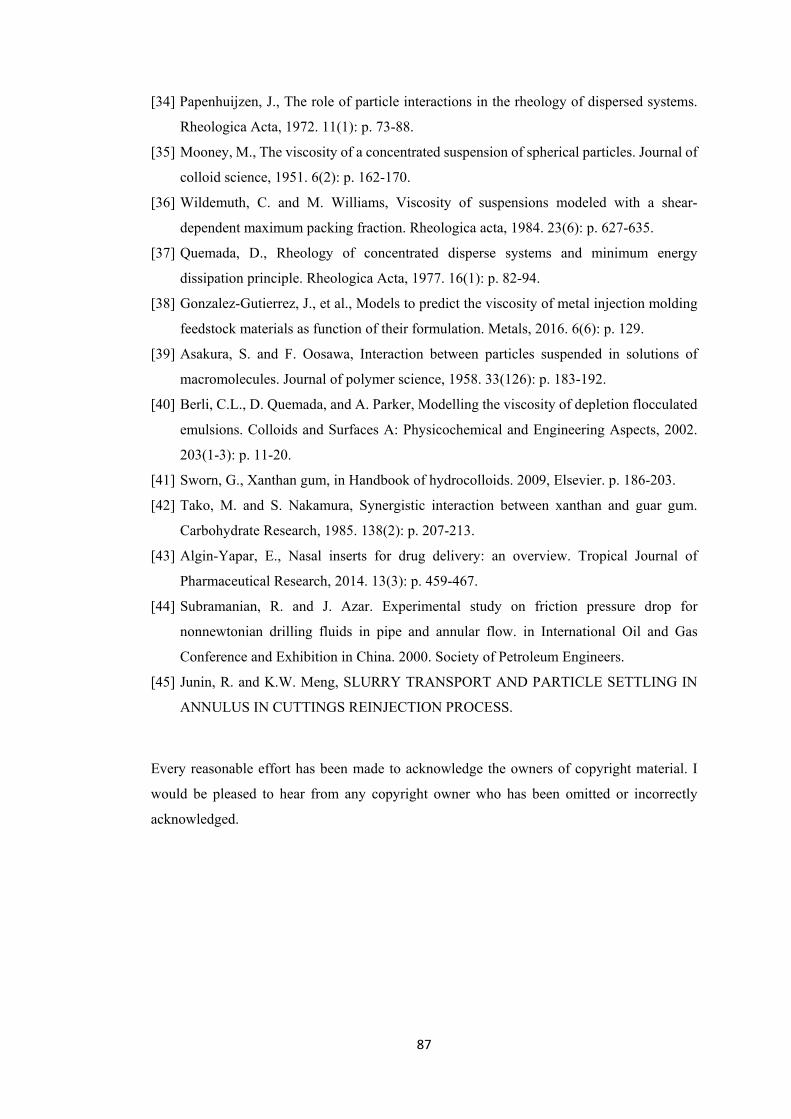
87
[34] Papenhuijzen, J., The role of particle interactions in the rheology of dispersed systems.
Rheologica Acta, 1972. 11(1): p. 73-88.
[35] Mooney, M., The viscosity of a concentrated suspension of spherical particles. Journal of
colloid science, 1951. 6(2): p. 162-170.
[36] Wildemuth, C. and M. Williams, Viscosity of suspensions modeled with a shear-
dependent maximum packing fraction. Rheologica acta, 1984. 23(6): p. 627-635.
[37] Quemada, D., Rheology of concentrated disperse systems and minimum energy
dissipation principle. Rheologica Acta, 1977. 16(1): p. 82-94.
[38] Gonzalez-Gutierrez, J., et al., Models to predict the viscosity of metal injection molding
feedstock materials as function of their formulation. Metals, 2016. 6(6): p. 129.
[39] Asakura, S. and F. Oosawa, Interaction between particles suspended in solutions of
macromolecules. Journal of polymer science, 1958. 33(126): p. 183-192.
[40] Berli, C.L., D. Quemada, and A. Parker, Modelling the viscosity of depletion flocculated
emulsions. Colloids and Surfaces A: Physicochemical and Engineering Aspects, 2002.
203(1-3): p. 11-20.
[41] Sworn, G., Xanthan gum, in Handbook of hydrocolloids. 2009, Elsevier. p. 186-203.
[42] Tako, M. and S. Nakamura, Synergistic interaction between xanthan and guar gum.
Carbohydrate Research, 1985. 138(2): p. 207-213.
[43] Algin-Yapar, E., Nasal inserts for drug delivery: an overview. Tropical Journal of
Pharmaceutical Research, 2014. 13(3): p. 459-467.
[44] Subramanian, R. and J. Azar. Experimental study on friction pressure drop for
nonnewtonian drilling fluids in pipe and annular flow. in International Oil and Gas
Conference and Exhibition in China. 2000. Society of Petroleum Engineers.
[45] Junin, R. and K.W. Meng, SLURRY TRANSPORT AND PARTICLE SETTLING IN
ANNULUS IN CUTTINGS REINJECTION PROCESS.
Every reasonable effort has been made to acknowledge the owners of copyright material. I
would be pleased to hear from any copyright owner who has been omitted or incorrectly
acknowledged.
88
Appendices Additives Data Sheet
Appendix A - AMC GUAR GUM

89
Appendix B - AMC PAC-R
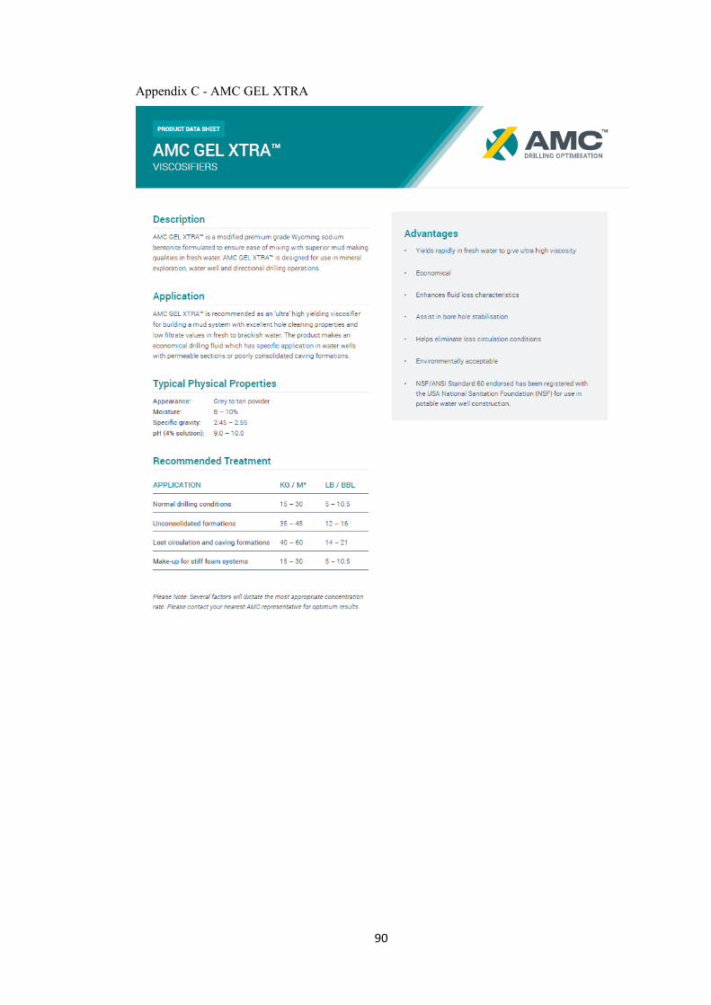
90
Appendix C - AMC GEL XTRA

91
Appendix D - COREWELL

92
Appendix E – AMC XAN BORE