study of steady-state wake characteristics of variable ... study of steady state wake...

Study of Steady-State Wake Characteristics

of Variable Angle Wedges

by

Grant Lee Eddy Jr.

Thesis submitted to the Faculty of the

Virginia Polytechnic Institute and State University

in partial fulfillment of the requirements for the degree of

MASTER OF SCIENCE

In

Mechanical Engineering

Commitee

P.S. King, Chairman W.F. O'Brien C.L. Dancey

September, 2001 Blacksburg, Virginia

Keywords: Wake, Inlet Distortion, Wedge, Transient, V-gutter, Gas Turbine Engine Testing

ii

Study of Steady State Wake Characteristics

of Variable Angle Wedges

by

Grant Lee Eddy Jr.

Committee Chair: P.S. King

Mechanical Engineering

Abstract

Current methods of creating inlet total pressure distortion for testing in gas turbine

engines are only able to simulate steady-state distortion patterns. With modern military

aircraft it is becoming necessary to examine the effects of transient inlet distortion on

engines. One alternative being evaluated is a splitting airfoil that is essentially a wedge

that can be set at different opening angles. An array of such devices would be placed in

front of the engine for testing that would be capable of creating steady-state distortion

patterns as well as transient distortion patterns by changing the opening angle of the

airfoils.

The work here analyzes the steady-state wake characteristics of some of the

splitting airfoil concepts. Single-wedge tests were conducted with various opening

angles in an attempt to classify the various aspects found in the wake pattern. It was

found that the wake has completely different characteristics with larger opening angles.

In addition, several different combinations of wedges were also examined to see if single

wedge analysis could be applied to arrays of wedges. Analysis was done on

combinations of wedges aligned vertically as well as combinations that were done

horizontally. It was found that single wedge characteristics change considerably when

different wake patterns interact with each other

iii

Acknowledgements

I would like to thank my advisory committee for the support and guidance that I

have received throughout my postgraduate education. Particular acknowledgement is

given to Dr. Peter King for aiding me in all aspects of my research even when there was

way too many things going on at times. Special gratitude is also given to Dr. King and

his wife Lorette for allowing me to stay in their home for the final month of my graduate

study. It really made things easier and was greatly appreciated.

I would like to thank Dr. Robertshaw and Dr. Diller for allowing me to be a

teaching assistant in various capacities so I was able to support myself while going

through graduate school. I would also like to thank Captain Sexton at VMI for

convincing me that graduate school was a good alternative.

A thanks goes to the Virginia Tech Machine Shop for building my test section and

supplying other items that were essential to my research. My apologies to Bill Songer for

breaking so many of your tools, but what else is a novice supposed to do.

The various people in the Turbolab past and present deserve some recognition

although most of them managed to leave before me. Scott, Karl, Matt, Drew, Keith,

Christian, and "Who let the Wayne out" are the departed and I wish them luck in their

endeavors. To Mac, Kevin, Joe, Jon and all the newcomers, I wish you luck in finishing

your graduate work and try not to save too much to do for the closing days.

A special thanks to the Richmond Crew for trying to make life a little easier at

times. "Slick Willy" deserves some special gratitude because I am sure he will be the

only one who will want to read this work of art.

I sincerely want to thank my girlfriend Marci Rapp for her support of me while I

was working on my postgraduate studies. Without her love and support, I probably

wouldn't have stuck it out till the end.

Last of all I would like to thank my parents and family for making sure I made the

right choices throughout life so far. You have been a great help in all my life so far and I

appreciate it.

iv

Table of Contents

Abstract ..............................................................................................................................ii

Acknowledgements...........................................................................................................iii

Table of Contents ............................................................................................................. iv

Table of Figures................................................................................................................vi

1 Introduction .................................................................................................................... 1

2 Literature Review........................................................................................................... 5

2.1 Current Inlet Pressure Distortion Practice ............................................................ 5

2.2 Transient Distortion Considerations ...................................................................... 8

2.3 Transient Distortion Generator Concept............................................................... 11

2.4 Splitting Airfoil Tests Completed .......................................................................... 17

3 Experimental Setup...................................................................................................... 23

3.1 Model Development ............................................................................................... 23

3.2 Wind Tunnel and Test Section............................................................................... 28

3.3 Testing Procedure.................................................................................................. 33

4 Test Results ................................................................................................................... 38

4.1 Flow Characteristics............................................................................................... 38

4.2 Single Wedge Results ............................................................................................. 41 Total Pressure Loss Contours.................................................................................... 42 Wake Width............................................................................................................... 47 Maximum Pressure Loss ........................................................................................... 50 Similarity Study......................................................................................................... 53 Summary ................................................................................................................... 55

4.3 Horizontally Aligned Wedge Results .................................................................... 56 Total Pressure Loss Contours.................................................................................... 57 Maximum Pressure Loss ........................................................................................... 63 Comparison with Single Wedge Data ....................................................................... 65 Summary ................................................................................................................... 68

4.4 Vertically Aligned Wedge Results ......................................................................... 69 Total Pressure Loss Contours.................................................................................... 70 Maximum Pressure Loss ........................................................................................... 80 Comparison with Single Wedge Data ....................................................................... 81 Prediction of Combination Data................................................................................ 85

v

Summary ................................................................................................................... 88

5 Conclusions and Recommendations .......................................................................... 90

5.1 Conclusions ........................................................................................................... 91

5.2 Recommendations .................................................................................................. 96

References ........................................................................................................................ 99

Appendix A-Wind Tunnel and Test Section Setup .................................................... 101

Appendix B - Percent Total Pressure Drop Contour Plots for Single Wedges ....... 105

Appendix C - Percent Total Pressure Drop Contour Plots for Combinations of Two Wedges Aligned Horizontally....................................................................................... 111

Appendix D - Comparison Plots for Horizontally Aligned Data .............................. 118

Appendix E - Percent Total Pressure Drop Contour Plots for Combinations of Two Wedges Aligned Vertically ........................................................................................... 125

Appendix F - Comparison Plots for Vertically Aligned Data ................................... 132

Appendix G – Uncertainty Analysis ............................................................................139

Vita.................................................................................................................................. 142

vi

Table of Figures Figure 1.1: Distorted and Undistorted Surge Lines............................................................ 3 Figure 2.1: Total Pressure Distortion Screens.................................................................... 7 Figure 2.2: Airjet Distortion Generator.............................................................................. 8 Figure 2.3: Splitting Airfoil Opened at Different Angles ................................................ 14 Figure 2.4: Array of Splitting Airfoils ............................................................................. 15 Figure 2.5: Possible Array of Splitting Airfoils .............................................................. 16 Figure 2.6: Jumel's Test Section Showing Measurements Taken at 1 ft., 2 ft., and 3 ft.

Behind the Wedge (Jumel, 1999).............................................................................. 18 Figure 2.7: Percent Total Pressure Loss Behind 60° Wedge (Jumel, 1999) .................... 20 Figure 2.8: Percent Total Pressure Loss Behind a 60° Wedge and a 90° Wedge at First

Station (Jumel, 1999) ................................................................................................ 21 Figure 3.1: Side view of hinge concept.......................................................................... 25 Figure 3.2: Original Hinge and Cut Hinge....................................................................... 26 Figure 3.3: Front and Rear of Actual Splitting Airfoil Tested ......................................... 26 Figure 3.4: Wind Tunnel and Test Section ...................................................................... 30 Figure 3.5: Traverse Used in Experiments....................................................................... 31 Figure 3.6: Plot of Electronic Manometer Calibration..................................................... 32 Figure 3.7: Total Pressure Measurements (1/8" and 1/4" increments) with a 60 Degree

Splitting Airfoil � Slot 2............................................................................................ 34 Figure 3.8: Front and Rear Views of 120° and 60° Airfoils in a Vertical Combination.. 36 Figure 3.9: Front and Rear Views of 120° and 60°Airfoils in a Horizontal Combination

................................................................................................................................... 37 Figure 4.1: Schematic Illustrations of Flow Regions of Wake and Jet Flow (Schetz,

1984).......................................................................................................................... 39 Figure 4.2: Flat Plate Structure Generating a Wake......................................................... 40 Figure 4.3: 3-D Total Pressure Drop Contour for a 60° Wedge at Slot 2 ........................ 43 Figure 4.4: 30° Airfoil Total Pressure Drop Contour at Slot 2 and Slot 7 ....................... 44 Figure 4.5: 90° Airfoil Total Pressure Drop Contour at Slot 4 and Slot 7 ....................... 45 Figure 4.6: 120° and 150° Airfoil Total Pressure Drop Contour at Slot 7....................... 46 Figure 4.7: Wake Width Definition Plots......................................................................... 48 Figure 4.8: Wake Width for Single Wedges .................................................................... 49 Figure 4.9: Maximum Pressure Loss Coefficient Varying with Distance for the Different

Wedge Angles ........................................................................................................... 51 Figure 4.10: Maximum Pressure Loss Coefficient Varying with Angle for the Distances

Downstream .............................................................................................................. 52 Figure 4.11: Nondimensional Vertical Pressure Loss Profile for Slots 2 and 7............... 54 Figure 4.12: Nondimensional Horizontal Pressure Loss Profile for Slots 2 and 7 .......... 55 Figure 4.13: 3-D Total Pressure Drop Contour for a 90° and 60° Wedge Aligned

Horizontally at Slot 2 ................................................................................................ 58 Figure 4.14: 60° and 90° Horizontally Aligned Airfoils Total Pressure Drop Contours at

Second Slot................................................................................................................ 59 Figure 4.15: 60° and 90° Horizontally Aligned Airfoils Total Pressure Drop Contours at

Third Slot................................................................................................................... 60

vii

Figure 4.16: 60° and 90° Horizontally Aligned Airfoils Total Pressure Drop Contours at Fourth Slot................................................................................................................. 61

Figure 4.17: 60° and 90° Horizontally Aligned Airfoils Total Pressure Drop Contours at Fifth Slot.................................................................................................................... 62

Figure 4.18: Maximum Pressure Loss Plots for Different Combinations of Airfoils Tested while Horizontally Aligned ........................................................................... 64

Figure 4.19: Typical Profile Locations for Comparison of Wedges for Horizontally Aligned Data ............................................................................................................. 66

Figure 4.20: Comparison of 60° and 90° with Horizontal Alignment to Single Wedge Data at Slots 2 and 3.................................................................................................. 67

Figure 4.21: Comparison of 60° and 90° with Horizontal Alignment to Single Wedge Data at Slots 4 and 5.................................................................................................. 68

Figure 4.22: 3-D Total Pressure Drop Contour for a 90° and 60° Wedge Aligned Vertically at Second Slot........................................................................................... 71

Figure 4.23: 60° and 90° Vertically Aligned Airfoils Total Pressure Drop Contours at Slot 2 ......................................................................................................................... 72








Figure 4.31: Maximum Pressure Loss Plots for Different Combinations of Airfoils Tested while Vertically Aligned ............................................................................... 80

Figure 4.32: Typical Profile Locations for Comparison of Wedges for Horizontally Aligned Data ............................................................................................................. 82

Figure 4.33: Comparison of 60° and 90° with Vertical Alignment to Single Wedge Data at Slots 2 and 5 .......................................................................................................... 84

Figure 4.34: Comparison of 30° and 120° with Vertical Alignment to Single Wedge Data at Slots 2 and 5.................................................................................................. 85

Figure 4.35: Superimposed and Original Contour Plots for a Combination of 60° and 90° Wedges at Slot 4 ................................................................................................. 87

Figure 4.36: Superimposed and Original Profiles for a Combination of 60° and 90° Wedges at Slot 4....................................................................................................... 88

Figure A1: Drawing of Wind Tunnel and Test Section ................................................. 102 Figure A2: Right Side View of Test Section.................................................................. 103 Figure A3: Left Side View of Test Section.................................................................... 103

viii

Figure A4: Second Left Side View of Test Section ....................................................... 104 Figure A5: View of Seven Slots on Test Section........................................................... 104 Figure B1: Single 30 Degree Wedge Total Pressure Drop Contours............................. 106 Figure B2: Single 60 Degree Wedge Total Pressure Drop Contours............................. 107 Figure B3: Single 90 Degree Wedge Total Pressure Drop Contours............................. 108 Figure B4: Single 120 Degree Wedge Total Pressure Drop Contours........................... 109 Figure B5: Single 150 Degree Wedge Total Pressure Drop Contours........................... 110 Figure C1: 30 Degree and 60 Degree Wedge (side-by-side) Total Pressure Drop

Contours .................................................................................................................. 112 Figure C2: 30 Degree and 90 Degree Wedges (side-by-side) Total Pressure Drop





Contours .................................................................................................................. 117 Figure D1: Comparison of 30° and 60° Wedges with Horizontal Alignment to Single

Wedge Data ............................................................................................................. 119 Figure D2: Comparison of 30° and 90° Wedges with Horizontal Alignment to Single





Wedge Data ............................................................................................................. 124 Figure E1: 30 Degree and 60 Degree Wedges (up and down) Total Pressure Drop

Contours .................................................................................................................. 126 Figure E2: 30 Degree and 90 Degree Wedges (up and down) Total Pressure Drop

Contours .................................................................................................................. 127 Figure E3: 30 Degree and 120 Degree wedges (up and down) Total Pressure Drop




Contours .................................................................................................................. 131 Figure F1: Comparison of 30° and 60° Wedges with Vertical Alignment to Single

Wedge Data ............................................................................................................. 133

ix

Figure F2: Comparison of 30° and 90° Wedges with Vertical Alignment to Single Wedge Data ............................................................................................................. 134





1

1 Introduction

The interaction between inlet flow uniformity and engine performance is an

important parameter in the field of aircraft turbomachinery. The ideal case would be if

the air entering the engine was uniform with a constant temperature, pressure and

direction. However, aircraft in flight rarely experience ideal flow into the engines. The

unsteady inlet flow that occurs can be caused by a number of things: maneuvers,

interaction of airframe and inlet, wakes from other aircraft, or gas ingestion from gun and

rocket exhaust [1]. All of these sources can produce a pressure or temperature distortion

that will create problems when the air is ingested into the engine. The effect on the

engine is that the available power is reduced, often causing the engine to experience

instability. Since the 1970s the gas turbine industry has been testing their engines to see

the effects of inlet distortion. At first, such testing was recommended, but over the last

25 years it has become an established practice [2].

All engine manufacturers use established guidelines for evaluating inlet and

engine performance with non-uniform airflow. These established methods are presented

in the Aerospace Recommended Practice, ARP-1420 [3] and its companion document,

the Aerospace Information Report, AIR-1419 [4]. These documents are mainly

concerned with total pressure distortion generated at the inlet. This is because total

pressure is capable of describing the distorted flow in enough detail to avoid performance

problems. These reports also discuss the distortion test methods, the data acquisition

system, and the recommended ways to assess performance and stability.

When pressure distortion is introduced into an engine it can have drastic effects

on the engine�s performance. The thrust and the power available can be greatly reduced

2

which means poor performance for the aircraft. In addition, the surge margin is reduced

which can lead to instability. Surge is defined as global oscillation of mass flow through

a compressor system, which can often lead to complete flow reversal [5]. The reason that

surge is a problem with a compressor is that the compressor is taking air at a lower

pressure and forcing it to a higher pressure, a situation in which the air naturally wants to

do the exact opposite. This reversal of natural events makes compressors inherently

unstable.

The surge line on a compressor map marks the locus of points where the engine

will experience instability, which can lead to violent oscillations in the engine. These

oscillations can cause unwanted blade vibration, which places unanticipated stress on the

blades. Blade stress can lead to replacement of the blades at an earlier time than planned.

These oscillations may even cause a blade to shear and to exit through the engine, which

is very disastrous and should be avoided at all costs. In the most extreme cases surge can

cause the air in the burner to exit through the compressor causing flames to come out the

front of the engine. Because compressor blades are not designed for that kind of heat and

stress, surge needs to be avoided as much as possible. Figure 1.1 shows a typical

compressor map with surge lines for distorted and undistorted flow. As can be seen in

Figure 1.1, the surge line is reduced with pressure distortion, limiting the available

performance of the engine.

3

Figure 1.1: Distorted and Undistorted Surge Lines

.

Davis et al. [2] discuss ARP-1420 and how surge margin and loss of surge

pressure ratio are major concepts incorporated. In ARP-1420 the surge margin is defined

as the difference between the surge pressure ratio and the operating pressure ratio,

normalized by the operating pressure ratio [3]. With the terminology of Figure 1.1, this

definition shows the undistorted surge margin (SM) to be

1001 ×−=PRO

PRO)(PRSM (1)

Engines are designed to operate well below the surge line although inlet pressure

distortion reduces the available surge margin pushing the engine towards surge. This loss

in surge pressure ratio due to inlet distortion ( ∆ PRS) is defined, with reference to Figure

1.1, as

1001

1 ×−=PR

PRDS)(PR∆PRS (2)

Operating Airflow

Operating Point

Distorted Flow

Surge Limit

Undistorted Flow

Surge Limit

Pressure

Ratio

Corrected Airflow

PR1

PRDS

PRO

4

Because the loss in surge pressure ratio needs to be minimized, it is the responsibility of

the designer to test their engines for inlet distortion to reduce surge margin. Engine

manufacturers must be able to test their engines with various distortion patterns in order

to avoid the effects of surge. AIR-1419 serves as a reference and guidance for testing the

effects of inlet pressure distortion.

There are several methods that engine manufacturers use today to test their

engines for pressure distortion. These methods are capable of testing the steady state

effect that distortion has on the aircraft components. The two most widely used methods

are distortion screens and airjet distortion generators. These methods will be discussed in

greater detail in Chapter 2. Today�s military aircraft are capable of extreme maneuvers

that can create distortion patterns that change rapidly. There is currently no effective way

to test engines for this transient pressure distortion. Therefore, alternate methods of

testing for inlet distortion need to be investigated that will address these transient

concerns.

5

2 Literature Review Gas turbine engine manufacturers have recognized the need for testing their

engines for performance in the presence of inlet distortion. It is important to keep the

engines away from surge to avoid performance loss and equipment failure. Engines are

tested for their response to temperature distortion and pressure distortion. Pressure

fluctuation before the inlet is a big concern since the compressor was designed for steady

flow. There are several established ways to create inlet distortion patterns to test the

effect on the engine components. These current methods are only able to simulate

steady-state distortion and are not capable of creating any transient distortion. Due to the

extreme maneuvers that modern military aircraft now perform, it is becoming necessary

to examine the current distortion techniques. It has been shown that transient distortion is

something that needs to be investigated. There has been some preliminary work on

looking at distortion generators capable of creating transient distortion. These studies are

far from complete and much more work needs to be done before transient distortion

devices can be used in industry.

2.1 Current Inlet Pressure Distortion Practice

Engine manufacturers follow several steps when testing their engines for

operations with inlet pressure distortion. The process normally starts with wind-tunnel

tests of subscale inlet and airframe components to provide some sort of measurement to

approximate the distortion. The next step is to use a direct-connect test, where a

component or engine is connected directly to an air supply duct that supplies conditioned

6

air at the same pressure, temperature, and Mach number experienced at a given flight

condition [2]. A distortion generator is then placed in the supply duct directly in front of

the engine in order to simulate the distortion found in the wind tunnel tests. The

distortion generator functions by creating a total pressure deficit that can then be assessed

on the different components of the engine. Currently two methods of distortion

generators exist: distortion screens and airjet distortion generators.

Distortion screens are the classical way that engines have been tested for

distortion effects. Screens were the first method used for creating distortion and are still

in use today. A distortion screen creates a physical blockage through wire mesh that

corresponds to a total pressure drop downstream. This flow blockage allows the screen

to generate steady-state total pressure distortion patterns. Each screen has only one

distortion pattern. As a result, many different screens are needed in order to simulate

more complex patterns. Each screen can have a different mesh and shape that can create

different distortion patterns. The distortion screen designs have been created through

years of testing engines for distortion. Typical patterns are circumferential, radial, or

combined since these are patterns that the aircraft will see in every day flight. Some

examples of distortion screens can be seen in Figure 2.1.

7

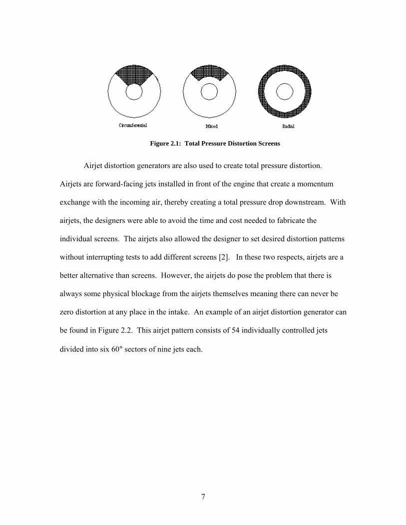
Figure 2.1: Total Pressure Distortion Screens

Airjet distortion generators are also used to create total pressure distortion.

Airjets are forward-facing jets installed in front of the engine that create a momentum

exchange with the incoming air, thereby creating a total pressure drop downstream. With

airjets, the designers were able to avoid the time and cost needed to fabricate the

individual screens. The airjets also allowed the designer to set desired distortion patterns

without interrupting tests to add different screens [2]. In these two respects, airjets are a

better alternative than screens. However, the airjets do pose the problem that there is

always some physical blockage from the airjets themselves meaning there can never be

zero distortion at any place in the intake. An example of an airjet distortion generator can

be found in Figure 2.2. This airjet pattern consists of 54 individually controlled jets

divided into six 60° sectors of nine jets each.

8

Figure 2.2: Airjet Distortion Generator

Airjet distortion generators and distortion screens are used for military and

commercial engines. Many of the distortion patterns will be the same for the two uses

such as take-off and landing. However, military aircraft have much greater

maneuverability and hence will see different distortion patterns than commercial engines

in certain instances.

2.2 Transient Distortion Considerations

Modern military aircraft are capable of very advanced maneuvers and designers

are always looking to create newer and better aircraft. These types of engines and

aircraft create new problems for distortion testing. The current distortion testing methods

are capable of simulating the distortion seen by aircraft only at moderate changes in angle

of attack (AOA) and sideslip. Moderate changes can be assumed to act as steady-state

distortion since there is no great shift from an ordered pattern. However, modern aircraft

are capable of changing AOA and sideslip at rates up to 50 deg/sec [6]. This high rate of

change from normal flight conditions can cause the inlet flow patterns to deviate from

9

steady-state, and the engine can become sensitive to the distortion pattern time history. It

takes somewhere on the order of one engine revolution for a pressure distortion to have

an effect on the compressor. Therefore, the transient distortion caused by extreme

maneuvers cannot be ignored.

There have been some tests performed to examine the effect of AOA on engine

performance. These tests were necessary because the F/A 18 aircraft had been

experiencing engine stalls at high angles of attack that were outside the flight envelope

[7]. Because, future fighter aircraft will be expected to routinely operate at these

conditions, the stall had to be investigated. A team of NASA and industry researchers

have developed the F/A-18A High Alpha Research Vehicle (HARV). This aircraft is a

F-18 that has been modified with a thrust vectoring vane system that provides the ability

to maintain high AOA conditions [8]. Tests were run to try to better understand the

effect of inlet distortion on the propulsion system at high AOA. As expected, the tests

showed higher levels of inlet distortion as AOA was increased. These tests did not take

into account any of the transient effects on engine stability that can be caused by rapid

changes in AOA . Instead, these tests showed that even at steady high AOA the engines

experienced stall due to increased circumferential pressure distortion.

Testing has also been done on variable geometry engine intakes to test for

transient distortion effects on the instability inception of a low-pressure compressor [9].

In this study, a LARZAC 04 twin-spool turbofan engine was operated and equipped with

a moving delta wing upstream of the engine that was capable of producing transient inlet

distortion. This experiment was important because aircraft with variable engine inlet

geometries are being built and flown today. The effect of this transient distortion was

10

studied to see what effect it had on the surge margin as compared to steady-state. It was

found that differences in the nature of stall inception existed. In general, the warning

times for engines approaching surge were greatly reduced with the introduction of

transient distortion. This study verified that transient distortion is something that needs to

seriously be considered in future engine and aircraft development.

In the current testing methods, transient variation and angular flow or swirl are

not considered important enough to be simulated. A numerical study was conducted on a

single high-speed rotor by Davis et al. [2] in order to see whether transient distortion and

swirl would have enough effect on the engine to change the experimental stall limit.

Transient distortion can be caused by rapid change in AOA and swirl can be caused by

serpentine inlet ducts that are being used in stealth operation. This investigation used a

code known as TEACC (Turbine Engine Analysis Compressor Code), which is a 3D

compression system code. A 90°, one-per-revolution, distortion pattern was simulated

using TEACC and the effect of the distortion on the compression system was found.

Next, rotation of the screen in the clockwise or counter-clockwise direction was

simulated. It was found with this changing distortion pattern that the stall margin was

lowered more than it would have been with steady-state distortion. Counter-rotating

swirl was found to have a much greater effect on the stability margin. This counter-

clockwise swirl can cause engine surge, even when the total pressure distortion appears to

be within allowable limits. Swirl and transient distortion both do have detrimental effects

on the engine stability, so the current test methods must be examined to address these

issues.

11

Airjet distortion generators and distortion screens are used to create steady-state

distortion. They are not used to create transient, or time variant distortion. This

limitation is adequate for commercial engines, but transient distortion effects are a large

concern for military aircraft. The current practice to test for transient distortion is to

measure the peak levels of distortion during the wind tunnel tests by looking at the time

history. These peak levels of distortion are then simulated using airjets or distortion

screens. This simulation does allow testing at peak distortion levels, but is still at steady

state. There is currently no good method to create transient pressure distortion patterns.

Several devices have been used to attempt to simulate time-variant distortion [2]. One

example is the random frequency generator which uses separated flow to produce

pressure fluctuations. Another example is a discrete-frequency generator which uses a

periodic pulsing of the flow to develop fluctuations. Neither of these methods have been

successful enough to be used in standard practice. Technology for aircraft engines is

continually advancing and in the future engines will require distortion generators capable

of producing rapid sequences of distortion patterns to provide a time history that could

represent a transient maneuver.

2.3 Transient Distortion Generator Concept

The U.S. Air Force Arnold Engineering Development Center (AEDC) has

recognized that transient distortion is something that must be addressed. The AEDC in

partnership with Virginia Tech has been developing technologies to provide controlled

transient pressure distortion [6]. This research focuses on creating new ways to generate

12

transient total pressure distortion patterns. Establishing the requirements of the distortion

generator was completed in Phase 1 of the current research. The distortion generator must

be capable of creating both classical and complex distortion patterns. Patterns that are

classified as classical are ones that all aircraft typically see in everyday flight such as

radial and circumferential distortion. Complex distortion patterns include the types of

distortion seen by aircraft attempting extreme maneuvers or those equipped with

serpentine inlet ducts. There are some additional requirements that the AEDC has

specified for distortion patterns, such as the pattern shapes generated by the device must

be characterized with magnitude and dimensions [6]. In addition, the distortion pattern

must correspond as closely as possible to those produced by transient maneuvers found in

fighter aircraft flight. These patterns must be controllable and repeatable. All of these

requirements must be satisfied in the new transient distortion generator.

Phase 2 was concerned with developing the new concept for creating transient

distortion. A literature review of the current distortion methods was completed by

DiPietro [10] to see if any of them could be altered to introduce transient distortion.

Distortion produced by physical blockage similar to screens and distortion produced by

momentum exchange like airjets was examined. Dipietro produced a list of fifteen

different concepts that were examined to find the best alternative. Some of these

concepts were variations of previous designs while some were new designs altogether.

After doing some analytical analysis, it was found that only five of the concepts

were suitable for further investigation. The two momentum exchange concepts involved

the use of air exchanging devices. One of the designs utilized streamlined airfoil struts

that were able to blow air into the airstream to create a momentum exchange. This design

13

was not that different from conventional airjets, but the streamlined struts would provide

very little distortion when the jets were off. The other design used suction on the airfoil

leading edge to obtain the pressure drop. The streamlined airfoil shape was chosen so that

the strut�s distortion was as minor as possible. The physical blockage concepts all used

mechanical obstructions to block the flow. One design was a flat plate that was able to

translate into and out of the duct perpendicular to the flow. In addition, this design was

also able to rotate to change angles of attack. Another design utilizing blockage was a

segmented blade concept. This design uses a flat plate that is at an angle to the flow.

The last design using blockage was the splitting airfoil design. This design is essentially

a wedge shaped device consisting of two flat plates that can be opened and closed to

different angles. The five different concepts were tested in a wind tunnel to see what

could be found about the total pressure loss.

During these tests a pitot static probe was scanned across the entire test section at

different intervals behind the distortion devices. The total pressure profiles of the

different designs were analyzed to see which option seemed to be the best choice. The

streamlined airfoil that sucked the air from the airstream was found to not cause enough

of a total pressure drop compared to the other designs. Therefore this design was

eliminated. The translating/rotating plate was found to cause distortion effects at all areas

of the test section. This would be a problem if a distortion pattern was needed only in the

center of a test section since this design would cause distortion at the outer edges also.

The splitting airfoil and segmented blade concepts were both able to produce controllable

pressure distortion. These concepts are essentially the same since the splitting airfoil is

just a mirror image of the segmented blade. The splitting airfoil may be the better design

14

since it will be easier to change the opening angle through the use of a hinge or similar

device. The splitting airfoil is also able to be fully closed which would give very little

distortion. The airjet momentum exchange device was also found to create favorable

total pressure patterns. Little distortion was found with the airjets turned off. Therefore

the best two devices were the airjet concept with streamlined struts and the splitting

airfoil design. Both of these devices were able to produce the desired free stream total

pressure distortion. In addition, both of these concepts were able to produce very little

distortion when in the �off� position.

It was decided that the physical blockage technique is a better concept to use than

momentum exchange. The physical blockage is easier and cheaper to use and is capable

of creating the distortion patterns needed. It was decided that a splitting airfoil device

would be the optimum design. This splitting airfoil was essentially a wedge that could be

opened to different angles to produce controlled distortion. The wedge is a symmetrical

bluff body that is capable of producing controlled and predictable distortion patterns. An

example of a splitting airfoil can be seen in Figure 2.3. In this figure the air is coming

towards the front of the wedge as indicated by the arrow. The distortion would be seen

downstream from the wedge.

flow

Figure 2.3: Splitting Airfoil Opened at Different Angles

15

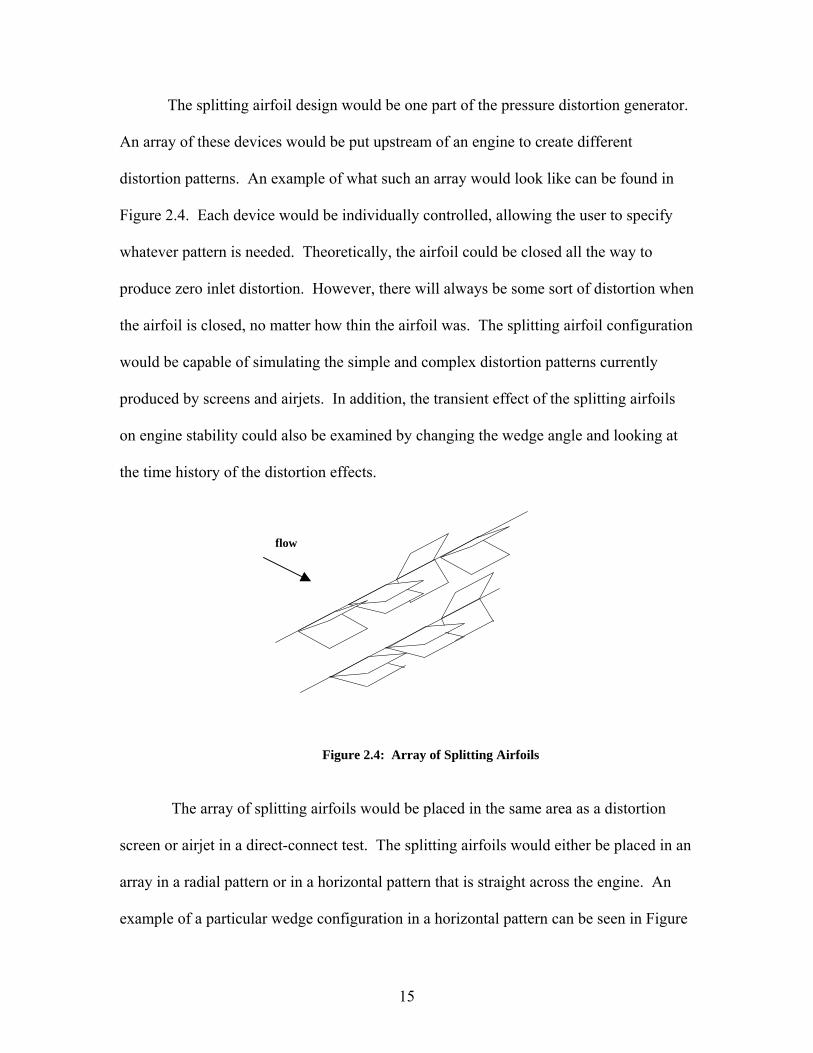
The splitting airfoil design would be one part of the pressure distortion generator.

An array of these devices would be put upstream of an engine to create different

distortion patterns. An example of what such an array would look like can be found in

Figure 2.4. Each device would be individually controlled, allowing the user to specify

whatever pattern is needed. Theoretically, the airfoil could be closed all the way to

produce zero inlet distortion. However, there will always be some sort of distortion when

the airfoil is closed, no matter how thin the airfoil was. The splitting airfoil configuration

would be capable of simulating the simple and complex distortion patterns currently

produced by screens and airjets. In addition, the transient effect of the splitting airfoils

on engine stability could also be examined by changing the wedge angle and looking at

the time history of the distortion effects.

flow

Figure 2.4: Array of Splitting Airfoils

The array of splitting airfoils would be placed in the same area as a distortion

screen or airjet in a direct-connect test. The splitting airfoils would either be placed in an

array in a radial pattern or in a horizontal pattern that is straight across the engine. An

example of a particular wedge configuration in a horizontal pattern can be seen in Figure

16

2.5. This is not necessarily a wedge pattern that corresponds to distortion levels that an

aircraft will ever see in flight. However, it is useful to show what patterns the model

distortion generator is capable of producing. The view of Figure 2.5 is from the front of

the engine looking at the wedge array. The fully blackened section represents places

where the splitting airfoil would be fully opened, while the small black areas represent

the areas where the splitting airfoils are partially opened.

Figure 2.5: Possible Array of Splitting Airfoils

The splitting airfoil concept is believed to be a possible candidate for the transient

total pressure distortion generator. Preliminary testing of the design was now needed to

ensure that pressure distortion created would be repeatable and large enough to be used in

testing.

17

2.4 Splitting Airfoil Tests Completed

Preliminary investigation of the splitting airfoil was completed by Jumel [10]

while working in the Turbomachinery Laboratory at Virginia Tech. His testing was not

concerned with trying to design the actual transient distortion generator, but was the first

step in trying to characterize the flow produced by such a device. Jumel tested several

different geometries of strut-mounted wedges in a wind tunnel to see what sorts of

distortion patterns were created. Each of his tests assessed the steady-state distortion

produced by one wedge. His goal was to see what the wake pattern looked like with

different angle wedges and to see how far downstream the patterns extended. He also

attempted to establish a control law that would enable the user to find the wake pressure

for different wedge geometries. However, the experimental results did not match the

theoretical predictions well, because of the unsteady flow mechanics associated with

bluff bodies.

Jumel was able to get some very interesting experimental data for different wedge

geometries. A view of his test section is shown in Figure 2.6. Data was collected at 1

foot, 2 feet, and 3 feet downstream of the wedge. The total pressure profile was

measured at each of these locations for different angles. He then determined the

turbulence index and the percent total pressure loss profiles. In order to assess the

pressure drop across the wedges, he used a pressure taken from upstream in the wind

tunnel. He also experimentally determined the wake pressure, which is a good indication

of how much distortion is being created. As expected, Jumel found that with increased

velocity and wedge angle the pressure drop increased.

18

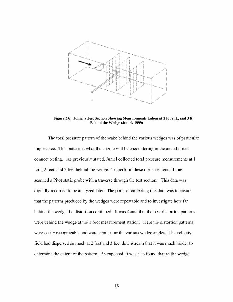
Figure 2.6: Jumel's Test Section Showing Measurements Taken at 1 ft., 2 ft., and 3 ft. Behind the Wedge (Jumel, 1999)

The total pressure pattern of the wake behind the various wedges was of particular

importance. This pattern is what the engine will be encountering in the actual direct

connect testing. As previously stated, Jumel collected total pressure measurements at 1

foot, 2 feet, and 3 feet behind the wedge. To perform these measurements, Jumel

scanned a Pitot static probe with a traverse through the test section. This data was

digitally recorded to be analyzed later. The point of collecting this data was to ensure

that the patterns produced by the wedges were repeatable and to investigate how far

behind the wedge the distortion continued. It was found that the best distortion patterns

were behind the wedge at the 1 foot measurement station. Here the distortion patterns

were easily recognizable and were similar for the various wedge angles. The velocity

field had dispersed so much at 2 feet and 3 feet downstream that it was much harder to

determine the extent of the pattern. As expected, it was also found that as the wedge

19

angle increased the distortion pattern increased as well. However, it was seen at the 1

foot station that the distortion pattern for different wedges showed similar characteristics.

An example of a distortion pattern can be seen in Figure 2.7. The plotted

parameter Cp is a pressure loss coefficient, and is represented by the following equation:

100(max)

)((max))( ×

−=

t

tt

PyPP

yCp (3)

In this equation )(yPt is the total pressure measured at each point in the grid, while

(max)tP is the maximum total pressure upstream of the wedge. In the figure, two

distinct zones can be seen that are characterized by peak total pressure loss. These zones

represent the symmetric area of the wedge and therefore should be nearly mirror images.

It is also interesting to note that the pressure loss induced by the strut holding the wedge

can be seen. The strut is shown as the horizontal region of pressure loss extending from

the wedge to the right wall. The strut did have some interaction with the wedge causing

some distortion that was not expected. Figure 2.7 shows a 60° wedge with total pressure

patterns measured at 1 foot, 2 feet, and 3 feet behind the wedge. It can be seen that as the

measurements are taken farther downstream of the wedge, the distortion pattern becomes

somewhat washed out and its boundaries are harder to specify. This result is because the

region of low pressure is dissipated as the flow progresses downstream. This dissipation

is shown to be much more extreme with increased wedge angle. However, it useful with

the small angle wedge here to see how the pattern dissipated and how the peak pressure

loss decreased.

20

1 Foot Behind Wedge 2 Feet Behind Wedge

3 Feet Behind Wedge

Figure 2.7: Percent Total Pressure Loss Behind 60° Wedge (Jumel, 1999)

Jumel�s results are somewhat misleading due to some uncommon assumptions

that were made in his analysis. After reviewing his data, it was found that the pressure

loss coefficients found using Equation 3 above were very high. Jumel had used the gage

pressure for (max)tP and for )(yPt . In the numerator this is fine since the difference

between the two values will still be the same. However, the absolute pressure is usually

used as the denominator to find the percent pressure drop. So what Jumel had found was

actually the percent gage pressure drop. Due to this fact, his values for the pressure loss

coefficient, Cp, as defined in this report, are actually much lower than the ones shown in

his figures. The patterns will still look the same although the values for his pressure loss

coefficient will be much lower, around 2 % at the maximum. Nevertheless, since it is his

100max

max ×−=Pt

PtPtCp

21

data that is being presented in this section, the plots will be given as they were in his

report even though some of the definitions were nonstandard.

Figure 2.8 shows a comparison of distortion patterns behind a 60° wedge and a

90° wedge taken one foot downstream. It can be seen that as the wedge angle increases

the size and depth of the distortion pattern also increases. It is also interesting to note that

the distortion pattern for the 90° wedge is getting close to being out of the range of the

graph. Due to the limitations of the traverse used in these experiments, Jumel was not

able to scan the entire test section. This limitation caused problems with the larger wedge

angles because the distortion pattern went beyond his traverse capabilities. For this

reason, some of the measurements that Jumel made at greater wedge angles did not show

the full distortion pattern, especially farther downstream from the wedge.

60° Wedge at Station 1 90° Wedge at Station 1

Figure 2.8: Percent Total Pressure Loss Behind a 60° Wedge and a 90° Wedge at First Station (Jumel, 1999)

Jumel showed with his testing that the splitting airfoil device is capable of

producing steady state distortion. The patterns produced by the wedges are consistent

and repeatable. It was found, as expected, that as the angle of the wedge increased, the

size and depth of the distortion pattern increased. The experiment also showed that the

22

best distortion patterns were found at one foot behind the wedge. At this location the

wakes were easily recognizable and similar for different wedge angles. This result

should give some indication of how far in front of the engine the eventual array of

splitting airfoils should be placed. At two and three feet behind the wedge, the total

pressure patterns were very washed out and hard to decipher. Future tests such as the

ones Jumel conducted should be centered around the area one foot behind the wedge or

closer. It is also necessary to analyze the pressure coefficient data in a more conventional

way. Jumel also was not able to get the complete pattern for some of the wedges at

higher angles due to traverse limitations. Any further testing should include an improved

traverse system so that it will be possible to scan the entire width of the test section.

Although Jumel did show that the splitting airfoil has definite promise for distortion

testing, his experimental setup was lacking in several respects.

23

3 Experimental Setup

It has been shown by Jumel and DiPietro that the splitting airfoil concept had

promise for a transient distortion generator. However, more investigation needed to be

done on the splitting airfoil concept. To accomplish this, a splitting airfoil design has

been built that is capable of being set at different angles. This enabled tests to be run with

different wedge angles while still using the same model. The tests were similar to

Jumel�s, being that the steady state total pressure loss was measured at several

downstream planes. After viewing Jumel�s results, it was decided that the current focus

should be on the first foot downstream. It was not known in this region how the wake

would form and interact with the free stream as it moved further downstream. In

addition, it was necessary to examine the entire width of the test section to get the

complete total pressure patterns. Also, combinations of more than one splitting airfoil in

close proximity were investigated. Combinations of airfoils were examined to see how

the wakes would interact with each other. This chapter will discuss the splitting airfoil

concept that was tested. It will also discuss the setup of the test section and will detail all

of the tests that were completed.

3.1 Model Development

It was necessary to create a splitting airfoil that would be capable of being set to

different angles between 0° and 180°. This device would have some sort of hinge to

enable the airfoil to open and close. Therefore, the best alternative was to use an existing

hinge to act as the airfoil. This would only approximate the actual device that would be

24

used in front of an engine, but would give test data to see what sort of pressure patterns

were capable of being created. The size of the hinge was chosen to be similar to the

wedge that Jumel studied so the results could easily be compared to each other. The size

of Jumel�s wedge was 1.5 inches along each edge and 1.5 inches wide. This would

correspond to an area that was 3 inches tall by 1.5 inches wide if fully opened. The

current investigation also focused on different configurations of airfoils that were tested

in the wind tunnel. The size of the airfoils used was decreased slightly compared to

Jumel�s so that the entire wake of the combination could be measured when testing more

than one prototype.

The size of the hinge that was decided on was a hinge that was approximately 2

inches tall and 1 inch wide when fully opened. This size was chosen to match Jumel�s

Reynolds number as close as possible while still allowing combinations of more than one

hinge to be examined. The pin for the hinge would also have to be removable to allow

the hinge to be placed on a strut in the test section. The best sort of hinge would be one

that gave the least amount of distortion when in the fully closed position.

A search was done of various hinge manufacturers to try and come up with a

suitable hinge. A collection of hinges was found at the McMaster-Carr Website [12].

The one that was chosen was a stainless steel hinge, model 1624A51. The dimensions of

this hinge were 2 by 2 inches and the thickness of the metal was 0.060 inches. The hinge

also had a removable pin. This hinge was the closest one that met all of the requirements.

When fully closed this hinge would have a height of 0.25" and 2" when fully opened.

This would enable as little distortion as possible when fully closed. A similar design

could be used in the actual direct connect testing, although the splitting airfoil would be

25

fitted with an actuation device. The hinge side view when fully closed and opened can be

seen in Figure 3.1.

Figure 3.1: Side view of hinge concept

This hinge needed to be cut down to get to the desired size of approximately 2

inches by 1 inch. Hinges are manufactured to have a curved circular metal section that

attaches the two different sides to the pin. One half of this particular hinge had 2 curved

sections while the opposite half had 3 curved sections. Therefore, in order to make the

hinge symmetrical, it was cut so there would be three of the curved sections in the final

design. After being cut, the size of the hinge was 2 inches tall and 1.125 inches wide.

Set screws were installed in the back of the hinge. These screws allowed the hinge to be

set to the angle that was needed for the different tests. The screws would be tightened

against the supporting rod that went through the hinge. A drawing of the original hinge

compared to the cut hinge can be seen in Figure 3.2. In addition, the actual splitting

airfoil used in the tests can be seen in Figure 3.3. Here you can see the set screws that are

in the back of the hinge.

26

Figure 3.2: Original Hinge and Cut Hinge

Figure 3.3: Front and Rear of Actual Splitting Airfoil Tested The rod that held the hinge in place was a 1/8" Diameter stainless steel rod. This

diameter was the same as the pin that had come in the original hinge, so no change

needed to be made to the hinges. It was necessary to calculate whether the rod would

27

bend from the force of the wind when placed in the test section. The hinge would have

the most force acting on it when open to 180°. At this angle the hinge could be treated as

a rectangular plate that is perpendicular to the flow. The drag would be the only force

acting on the hinge when fully opened and the formula for the drag is shown by the

following equation:

A*U*ρ*C*21Drag 2

d= (4)

where

Cd= drag coefficient ρ= density U= velocity A= area

Blevins [13] gives the drag coefficient, Cd, for a flat plate perpendicular to the

flow for the size of this hinge to be 1.10. The density was calculated from atmospheric

conditions when the tests were run. The tunnel free stream velocity was the same as

Jumel�s wind tunnel tests, 42 meters per second. The drag for a single hinge was

calculated to be 1.56 N. During the tests, the maximum number of airfoils that would be

on any one rod at one time would be two. Therefore the max force acting on the rod

would be 3.13 N. In order to find if the rod would bend, it was treated as a beam

supported at both ends with the max load at the center. Mott [14] gives the formula for

maximum deflection with this type of beam and loading as:

I*E*48

L*Wδ3

= (5)

28

where δ= deflection W= force acting in center of beam L= length E= modulus of elasticity I= moment of inertia

With all of these values known for the steel rod, it was found that the deflection

would be less than 1/16th of an inch at the worst case. In reality it wouldn�t even flex this

much because the force would not be acting in the middle of the rod and no tests were run

with the splitting airfoil open all the way. Therefore the rod was stiff enough to be used

for holding the splitting airfoil in the test section.

3.2 Wind Tunnel and Test Section

This section will describe the wind tunnel and test setup that were used in the

experiments. More details, including drawings and pictures of the test setup can be found

in Appendix A.

All information given below about the wind tunnel came from Jumel�s report

previously mentioned [11]. The wind tunnel used was originally designed and built by

Tkacik [15] for his experiments on stalled flow. It uses a centrifugal blower built by the

Aerovent Corp. (model BIA, size 630, class II). The fan is equipped with a 15

horsepower electric motor. The inlet area can be adjusted by moving the inlet guide vanes

which subsequently control the velocity. When originally designed, the tunnel could

produce velocities from 15 m/s to 48 m/s. However, the maximum velocity that can

currently be reached is approximately 42 m/s. A honeycomb (8,000 cells, 76.2 mm thick)

29

and 3 screens are installed in the 1.2 square meter settling section. This honeycomb helps

to reduce the freestream turbulence level in the flow prior to entering the nozzle. The

nozzle accelerates the flow and reduces the area of the tunnel from 0.836 2m to

0.093 2m , before the test section. This area reduction decreases the boundary layer

thickness at the entrance of the test section. The exit of the tunnel is 12" by 12" and has a

mounting flange at the exit.

A test section was constructed out of ½ " thick Lexan , a clear acrylic material.

The inside dimensions of the test section was 12" by 12" to match the exit of the wind

tunnel. The test section was 40 inches long and had a flange on one end to attach it to the

wind tunnel exit. A ¼" hole was cut 4 inches from the beginning that was used for a Pitot

static probe used to measure the inlet conditions. Tests were run on single hinges and

combinations of two hinges, positioned on top of each other and side to side. Three holes

were drilled on either side of the test section to allow the rods to be placed so the

different combinations of hinges could be tested. There were seven ¼" inch slots cut

across the width of the top of the test section. These slots were used for the Pitot probe to

scan the area inside. The first slot was placed so that the sensing end of the probe was 1�

behind the rod holding the hinge. The slots then continued every 2 inches downstream

for a distance of 13 inches behind the hinge, for a total of seven slots. This would allow

for measurements at 1,3,5,7,9,11,and 13 inches downstream of the airfoil. A picture of

the test section and wind tunnel can be seen in Figure 3.4.

30

Figure 3.4: Wind Tunnel and Test Section

A traverse was used to allow the pitot tube to scan the entire section. This was a

student-made traverse that was manually positioned. This traverse was located on top of

the test section and the probe was fed through the slots that were cut there. The traverse

could be moved from slot to slot to measure different downstream stations. This traverse

was able to scan the entire area of the test section. The horizontal and vertical position of

the probe could be set manually using two hand cranks. A picture of the traverse can be

found in Figure 3.5.

31

Figure 3.5: Traverse Used in Experiments

There were two pressure probes used to collect data. A Pitot-static probe was

used that was placed 4 inches from the inlet. This was used to capture the inlet

conditions, including inlet total pressure and inlet differential pressure. There was also a

Pitot probe attached to the traverse. This probe was used to capture the steady state total

pressure in the wake behind the splitting airfoil. These pressure patterns were the focus

of this study.

The probes were connected to a pressure transducer by flexible neoprene tubes.

The transducer used was a Datametrics Barocel Type 590D-10W-2PI-V1X-4D that was

capable of measuring differential pressures up to 10 inches of water. To get the

differential pressure upstream the tubes from the pitot-static probe were attached to high

and low ends of the pressure transducer. For the total pressure measurements, both

probes were attached individually by tubes to the high pressure end and the were

referenced to ambient pressure. The pressure transducer was linked to a Type 1400

Electronic Manometer that read in inches of water. This arrangement allowed pressure

measurements accurate to 0.001 inches of water. The voltage from the manometer was

32

input to a National Instruments Data Acquisition box that was linked to a laptop through

a data acquisition card (type A1-16E-4). Labview software was used to analyze the

transducer signal. The data acquisition system was set up to have a low pass

Butterworth Filter with a cutoff frequency of 100 Hz . Data was collected at 10,000

scans/sec every 3 seconds. The output voltage from Labview was displayed on the laptop

and the corresponding pressure values were input into a spreadsheet.

The barocel pressure transducer was calibrated against an inclined manometer

containing red gauge oil. Voltage from the electronic manometer was compared to the

pressure reading from the inclined manometer. A linear regression was used to obtain the

line fitting of the calibration data, as shown in Figure 3.6. It was found that the

relationship between voltage and pressure read on the electronic manometer was 1-1.

Figure 3.6: Plot of Electronic Manometer Calibration

Electronic Manometer Calibration

0

1

2

3

4

5

6

7

8

9

10

0 1 2 3 4 5 6 7 8 9 10

Inclined Manometer Reading (in. H20)

Elec

tron

ic M

anom

eter

Rea

ding

(vol

ts)

readingsLinear (readings)

33

3.3 Testing Procedure

This section will outline the testing procedure and will explain all of the tests that

were completed. In addition, an uncertainty analysis for all of the measurements that

were taken can be found in Appendix G. The first step was to remove the test section

from the wind tunnel. Next the airfoil or airfoils were placed in the test section. The

opening angle was set with a protractor and then the set screws were tightened. To make

sure that the airfoils were aligned correctly in the tunnel, a metal square was used. The

square was placed with one edge on the bottom wall of the section and the rod holding

the airfoil was rotated until the trailing edges of the airfoil were flush with the vertical

portion of the square. The test section was then attached to the wind tunnel by the use of

6 C-clamps that attached the two flanges. The traverse was then placed on top of the test

section at whichever distance was being investigated.

Before each test was started, the atmospheric pressure was recorded. After

starting the wind tunnel, the inlet total pressure and differential pressure given by the

pitot-static probe were recorded. The pitot probe was then used to scan the entire test

section in 1/4" intervals. The total pressure profile at each distance was recorded. After

completing each test the inlet conditions were recorded again. The test was then repeated

at each downstream slot.

Before data collection had begun, a sample test was completed to see if 1/4"

sampling intervals would be sufficient to get meaningful data. A 60° airfoil was placed

in the tunnel and total pressure measurements at the second slot were taken at 1/4" and

1/8" intervals. The resulting plots of total pressure for the bottom half of the wedge can

be seen in Figure 3.7. It can be seen from these plots that while there is slightly better

34

resolution with the 1/8" increments, the shape and depth of the distortion pattern is

essentially still the same with 1/4" increments. Therefore, 1/4" increments were used for

all of the testing.

Figure 3.7: Total Pressure Measurements (1/8" and 1/4" increments) with a 60 Degree Splitting Airfoil – Slot 2

No tests were run on the splitting airfoil when it was completely closed or when it

was open all the way to 180°. The angles that were investigated were 30°, 60°, 90°, 120,

and 150°. These angles refer to the total included angle of each airfoil. It was discovered

that at 1" behind the airfoil, (first slot), it was not possible to take data at the smaller

angles. This was due to the fact that the clearance was so small that the probe would

make contact with the trailing edge of the hinge. Therefore, no tests at any angles were

completed at this distance. During testing, all of the slots other than the one being

investigated were covered so that no flow could enter or leave the test section.

5 5.5 6 6.5 7Distance (inches)

4.5

5

5.5

6

Dis

tanc

e(in

ches

)

Pt (in./H2O

3.722223.166672.611112.055561.5

60 Degree Airfoil - Slot 21/8" Increments

5 5.5 6 6.5 7Distance (inches)

4.5

5

5.5

6

Dis

tanc

e(in

ches

)

Pt (in./H2O)

3.722223.166672.611112.055561.5

60 Degree Airfoil - Slot 21/4" Increments

35

For single wedges, steady state total pressure measurements were taken at slots 2-

7 for all five angles. This gave a good representation of how the wake developed

downstream. There were combinations of wedges tested also. Combinations of two

wedges mounted vertically and two wedges mounted horizontally were tested. It was

decided that no tests needed to be completed with two wedges having the same angle

since the wake pattern was already known from the single wedges and it was anticipated

that the wake would look the same for combinations with the same angle. It was also

decided that it would not be useful to test wedge combinations that would be the same

reversed, for example 30°-90° side by side and 90°-30° side by side. The pattern would

still look the same but reversed. That left ten combinations of different wedge angles.

After much of the testing it was decided not to do tests with the 150° angle wedge since

the other combinations gave enough data to determine what would happen with arrays of

two airfoils. Table 3.1 shows the possible combinations of two airfoils that could have

been tested. Here X marks the duplicate combinations, ------ marks the combinations

with the same angle, and the ! marks the combinations that were tested.

30 60 90 12030 ------------ X X X60 ! ------------ X X90 ! ! ------------ X

120 ! ! ! ------------

Table 3.1 Possible Combinations of 2 Wedge Angles

A combination of two wedges was tested with one on top of the other. There was

a 1/4" vertical gap between adjacent airfoils when fully opened. This was done since it

36

was anticipated that a similar spacing would probably be used in the actual array of

airfoils. The airfoils were aligned so both were in the middle of the test area and were

horizontally in the same position. With this arrangement, measurements were taken at

slots 2-5, skipping slots 6 and 7. It will be shown later in this report that this was

sufficient distance before the two wakes merged too much to distinguish the two. Front

and back views of a combination of two airfoils aligned vertically can be seen in Figure

3.8.

Figure 3.8: Front and Rear Views of 120° and 60° Airfoils in a Vertical Combination

Combinations with two wedges side by side were also tested. There was also a

1/4" gap between adjacent airfoils in this setup. This was done to be consistent with the

gap that was in place with the vertical tests. Data was also taken with this arrangement at

slots 2-5. Front and rear views of a combination of two airfoils aligned horizontally can

be seen in Figure 3.9. In both of these photographs the larger angle airfoil is 120° while

the smaller angle measures 60°.

37

Figure 3.9: Front and Rear Views of 120° and 60°Airfoils in a Horizontal Combination

All of the data taken was entered into a spreadsheet for analysis. The following

chapter will give the results that were found with these experiments and will discuss the

analysis that was done.

38

4 Test Results This chapter will present the results from the data that was collected for the

various tests discussed. These results will be for single airfoils and combinations of two

airfoils aligned horizontally and vertically. Prior to discussing the results, a section on

the characteristic wake flow is given. This section helps to explain the results by

showing the specific characteristics that this type of flow will show.

4.1 Flow Characteristics The splitting airfoil design tested is a wedge-shaped bluff body that creates a

wake downstream. A wake is defined as a deficit of momentum and energy behind a

body in a fluid flow [13]. This drop in momentum is evidenced by a decrease in velocity

and total pressure. The wake is formed when the flow separates at the trailing edges of

the airfoil. These separation streamlines form a shear layer between the faster free stream

and slower moving fluid. The area within the shear layers is the wake. The symmetry of

a wedge prevents the two shear layers from interacting until very far downstream. The

wake that is formed moves downstream until eventually it dissipates back into the free

stream.

Wakes are often grouped together with jets for analysis purposes. A jet is a

source of energy and momentum and a wake is a deficit of energy and momentum.

However, they do exhibit many of the same characteristics. Such as, there is no rigid

surface present in the region of interest and the wall-dominated region is eliminated.

39

Wakes and jets both exhibit several different regions as the flow progresses downstream

[16]. The near wakes directly behind a bluff body or the potential core directly

downstream of a jet are very complex regions. The shape of these areas is governed by

the shape of the body or jet. The region far downstream from a jet or body is called the

similarity region and analysis is easier there because wake or jet profile is fully

developed. The flow is classified as being in the similarity, or far wake region if the

difference between the free stream velocity and the wake velocity is small. Between the

near wake and far wake region is the transition region, where the flow is continuously

changing and developing. These two regions of flow are seen in Figure 4.1. The bluff

body in this case is a cylinder, but similar characteristics are seen for a wedge shaped

bluff body.

Figure 4.1: Schematic Illustrations of Flow Regions of Wake and Jet Flow (Schetz, 1984)

40

Blevins [13] describes these flow regions for a bluff body with a turbulent wake.

The near wake region bears an imprint of the structure generating the wake. This near

wake region is often unsteady due to periodic shedding of eddies. These near-wake

eddies are associated with a low-pressure region. Approximately 200 characteristic

diameters downstream, the eddies are obliterated and steadier flow continues. Here is the

similarity region discussed by Schetz. The near wake and far wake patterns described by

Blevins are shown in Figure 4.2 for a flat plate structure parallel to the flow.

Figure 4.2: Flat Plate Structure Generating a Wake

Studies have been done on V-shaped bluff bodies by Yang et al [17]. In these

tests the working fluid was high velocity air. In addition, the wedge shape extended

across the entire test section so that a 2-D analysis would be sufficient. It was found that

the vortex shedding that occurred in the shear layer had a close interaction with the wake

structure. Goldstein [18] also discussed how the fluid in the wake is separated from the

free flow by vortex layers in the boundary layer that formed at the point of separation.

This vortex shedding was high frequency but relatively weak. It was also seen that

vortices were formed in the wake itself. The vortices were formed on either trailing edge

and interacted further downstream forming other vortices. The vortices are alternately

discharged from the two sides and form a double row with the point separating these

41

vortices being the middle of the wedge shaped bluff body. At higher Reynolds numbers

it becomes harder to visualize the vortex pairs.

Three-dimensional bluff bodies introduce even more complicated flow

characteristics. In the tests completed the flow is definitely 3-D since the free stream is

able to interact with the wake on all sides of the wedge. In 3-D flow there is boundary

layer detachment on the trailing edges of the top and bottom of the airfoil and also

boundary layer detachment at the side of the body [11]. The vortices formed here can

create mean swirl velocity and can have strong axial components and important effects

downstream. Indeed, it will be seen later that at higher angles the wedges are influenced

by the boundary layer detachment on the sides and the wake patterns spread in the

horizontal direction. All of these flow characteristics for wedge shaped bluff bodies will

help to explain some of the results that will be discussed.

4.2 Single Wedge Results

This section will detail all of the results for the single wedge data with different

opening angles. The total pressure loss contours will be discussed first. Emphasis will

be placed on how the wake pattern for different angles develops as the flow progresses

downstream. The width of the wake will be investigated as will the maximum pressure

loss for the different wedges. Finally, the wedge wake patterns will be compared to each

other in an attempt to find some correlation between different wedge angles and

downstream development.

42

Total Pressure Loss Contours Total pressure data was taken for the five different test angles at slots 2-7, i.e.

planes of total pressure at 3", 5", 7", 9", 11" and 13" downstream. The pressure loss

coefficient, Cp, was calculated across each plane in order to help assess the total pressure

drop. The formula for the pressure coefficient is the same as given before:

100(max)

)((max))( ×

−=

t

tt

PyPP

yCp (3)

All of the values used are absolute pressures, since this was necessary to get the actual

percent pressure drop. The maximum total pressure was found in the free stream in the

inlet upstream of the wedge. The error analysis for this calculation can be seen in

Appendix G. Contour plots were made that showed the percent total pressure loss

profiles in the wedge wake. The complete set of contour plots for all of the single

wedges tested at the different slots can be found in Appendix B.

Before discussing any of the patterns for the different wedges it is useful to look

at a 3-D contour plot. On the 2-D plots, the pressure drop from the rod holding the

airfoils can clearly be seen. Compared to the pressure drop from the airfoil, the rod has

very minor differences from free stream. This can best be seen in a 3-D contour plot.

Figure 4.3 shows such a 3-D plot for a 60° wedge at slot 2. While the rod holding the

hinge can be seen, it is also shown that the pressure drop is very minor compared to the

actual wedge wake.

43

0

0.5

Cp(

%)

45

67

8 Distance (inches)

4

5

6

7

8

Distance(inches)

Cp(%)1.51.3751.251.12510.8750.750.6250.50.3750.250.1250

60 Degree Wedge - Slot 2

Figure 4.3: 3-D Total Pressure Drop Contour for a 60° Wedge at Slot 2

In the final design, there will be a support structure that holds the splitting airfoils

in an array in front of the engine. This support should be a streamlined strut rather than a

circular rod that is holding these wedges. For a circular bluff body, it can be seen that the

flow around the rod is not greatly affecting the wake pattern. A streamlined strut will

affect it even less. This is a positive thing since the support strut or rod is not wanted to

disturb the flow or wake pattern since distortion is only wanted from the airfoils.

At smaller angles the wake pattern stayed very similar as the flow dispersed

downstream. With progression downstream, the pressure loss decreased and the wake

became larger. However, the same pattern with the two distinct areas of peak pressure

drop could be seen at all distances. The 3-D effect did not play an important role in small

angle airfoils since little flow entered the wake pattern from the side to cause the two

peaks to vanish. This is the same type of pattern that Jumel saw when he analyzed his

test data for small angles. The 30° and the 60° angle airfoils both exhibited this behavior.

44

Figure 4.4 shows the percent total pressure drop contour for a 30° angle airfoil at slots 2

and 7. It can be seen that the wake pattern showed similar patterns as the flow progressed

downstream. The intensity of the maximum pressure loss was decreased by nearly 70%

from slot 2 to slot 7. The wake width in the vertical direction increased by nearly 100%.

This behavior was also representative of that found with the 60° airfoil.

Figure 4.4: 30° Airfoil Total Pressure Drop Contour at Slot 2 and Slot 7 Figure 4.5 shows a 90° airfoil at slots 4 and 7. The behavior was different for

larger airfoil angles. At 90° and above the wake patterns did not stay the same shape as

they progressed downstream. Instead, the wake dispersed in the horizontal direction. For

the 90° airfoil the two distinct zones of maximum pressure drop on either side of the

support rod could be seen at slots 2-4. At slots 5-7 these distinct zones disappeared and

instead the maximum pressure loss moved to two lobes on either side of the airfoil while

the height remained nearly the same. This shift was most likely caused from the two

vortices on the top and bottom of the wedge interacting with each other and combining to

form a higher velocity at the center and a smaller velocity towards the outside where the

4 5 6 7 8Distance (inches)

3.5

4

4.5

5

5.5

6

6.5

7

7.5

8

Dis

tanc

e(in

ches

)

Cp(%)1.51.3751.251.12510.8750.750.6250.50.3750.250.1250

Slot7


3.5

4

4.5

5

5.5

6

6.5

7

7.5

8

Dis

tanc

e(in

ches

)

Cp(%)1.51.3751.251.12510.8750.750.6250.50.3750.250.1250

Slot 2

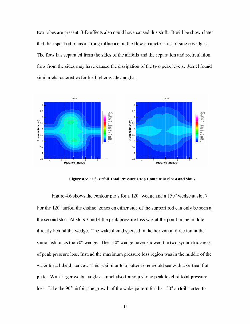
45


3.5

4

4.5

5

5.5

6

6.5

7

7.5

8

Dis

tanc

e(in

ches

)

Cp(%)1.51.3751.251.12510.8750.750.6250.50.3750.250.1250

Slot 4


3.5

4

4.5

5

5.5

6

6.5

7

7.5

8

Dis

tanc

e(in

ches

)

Cp(%)1.51.3751.251.12510.8750.750.6250.50.3750.250.1250

Slot 7

two lobes are present. 3-D effects also could have caused this shift. It will be shown later

that the aspect ratio has a strong influence on the flow characteristics of single wedges.

The flow has separated from the sides of the airfoils and the separation and recirculation

flow from the sides may have caused the dissipation of the two peak levels. Jumel found

similar characteristics for his higher wedge angles.

Figure 4.5: 90° Airfoil Total Pressure Drop Contour at Slot 4 and Slot 7

Figure 4.6 shows the contour plots for a 120° wedge and a 150° wedge at slot 7.

For the 120° airfoil the distinct zones on either side of the support rod can only be seen at

the second slot. At slots 3 and 4 the peak pressure loss was at the point in the middle

directly behind the wedge. The wake then dispersed in the horizontal direction in the

same fashion as the 90° wedge. The 150° wedge never showed the two symmetric areas

of peak pressure loss. Instead the maximum pressure loss region was in the middle of the

wake for all the distances. This is similar to a pattern one would see with a vertical flat

plate. With larger wedge angles, Jumel also found just one peak level of total pressure

loss. Like the 90° airfoil, the growth of the wake pattern for the 150° airfoil started to

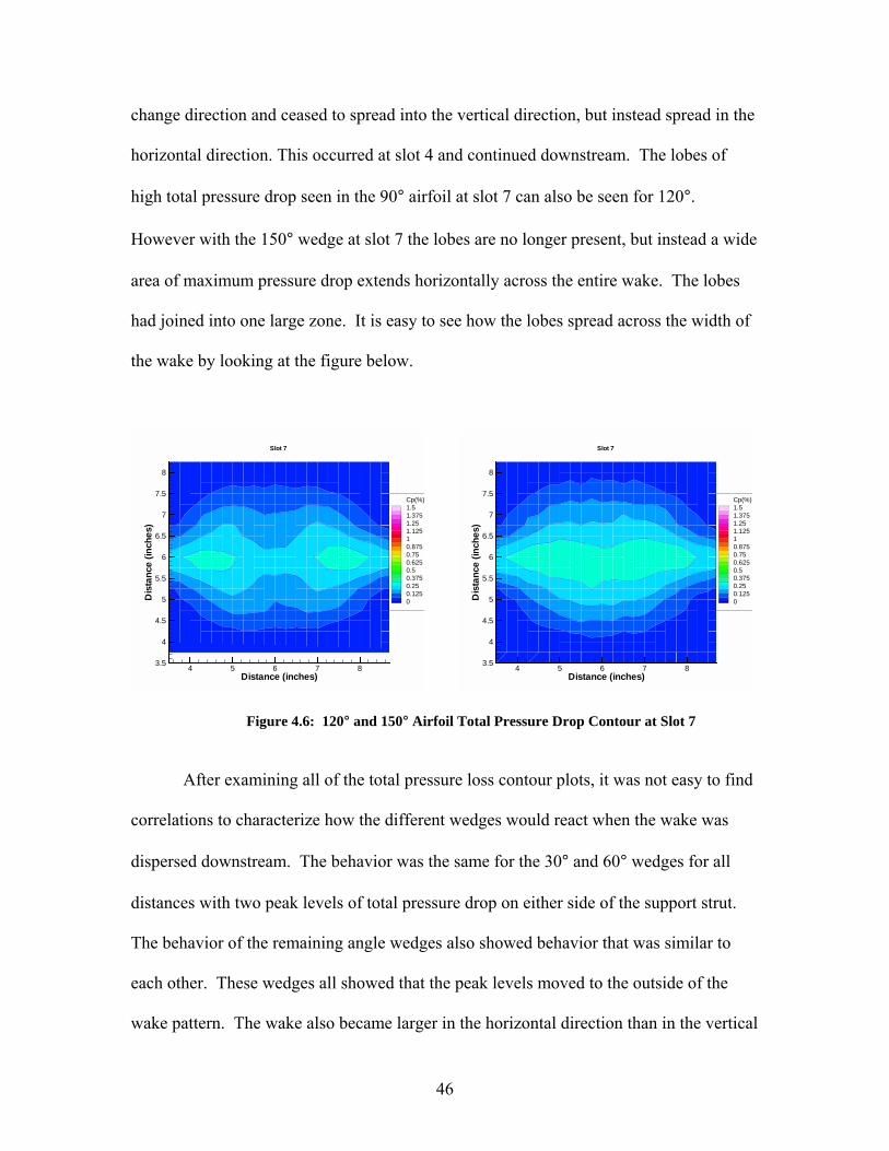
46

change direction and ceased to spread into the vertical direction, but instead spread in the

horizontal direction. This occurred at slot 4 and continued downstream. The lobes of

high total pressure drop seen in the 90° airfoil at slot 7 can also be seen for 120°.

However with the 150° wedge at slot 7 the lobes are no longer present, but instead a wide

area of maximum pressure drop extends horizontally across the entire wake. The lobes

had joined into one large zone. It is easy to see how the lobes spread across the width of

the wake by looking at the figure below.

Figure 4.6: 120° and 150° Airfoil Total Pressure Drop Contour at Slot 7

After examining all of the total pressure loss contour plots, it was not easy to find

correlations to characterize how the different wedges would react when the wake was

dispersed downstream. The behavior was the same for the 30° and 60° wedges for all

distances with two peak levels of total pressure drop on either side of the support strut.

The behavior of the remaining angle wedges also showed behavior that was similar to

each other. These wedges all showed that the peak levels moved to the outside of the

wake pattern. The wake also became larger in the horizontal direction than in the vertical


3.5

4

4.5

5

5.5

6

6.5

7

7.5

8

Dis

tanc

e(in

ches

)

Cp(%)1.51.3751.251.12510.8750.750.6250.50.3750.250.1250

Slot 7


3.5

4

4.5

5

5.5

6

6.5

7

7.5

8D

ista

nce

(inch

es)

Cp(%)1.51.3751.251.12510.8750.750.6250.50.3750.250.1250

Slot 7

47

direction for all angles 90° and larger. To try to classify the size of the individual

patterns the wake width was investigated next.

Wake Width It is useful to use the wake width as a parameter to see how the size of the wake

pattern changes as the flow progresses downstream. It has been shown that the flow

pattern of a jet has very much in common with the wake pattern from the splitting airfoil

design. Therefore, the terminology for jet width will be used with the splitting airfoil

wake. Schetz [16] uses the half radius as the characteristic width for a jet. The half

radius is defined as the distance where the velocity is half of the maximum jet velocity.

In this analysis, the half width is defined as the width between the two points where the

pressure loss coefficient is half that found at the maximum point. The wake width needs

to be investigated in the horizontal and vertical direction due the axis switching that

occurs with higher angle wedges. For vertical width, a slice of the total pressure contour

plots was taken from the center of the wedge where the distortion was presumed to be the

strongest. It was then possible to find the points on the curve where the pressure loss

coefficient was half that of the maximum value. These values were interpolated from the

data to find the actual height.

Figure 4.7 shows this more clearly. This figure is of a 30° wedge wake at slot 2.

In the plot on the left, it can be seen where the slice of the total pressure loss coefficient

was taken. The plot on the right shows the view of the total pressure loss profile and the

points used to calculate the half width. This method of finding the width was used for

vertical and horizontal distances. For the horizontal width, a slice of the pressure loss

48

contour was chosen that would give a good representation of what the plot looked like

across the horizontal axis.

Figure 4.7: Wake Width Definition Plots

Just showing a plot of the wake width in the vertical or horizontal direction is not

a good representation of how the pattern changes. Due to the fact that the major axis

switched with the larger angle wedges, a different way of showing the wake width was

needed. This axis switching is similar to behavior that is seen by elliptical jets, which

often switch the major axis as the flow progresses downstream. In his studies on

elliptical jets, Mutter used an equivalent jet radius, eR , given as [19]:

baRe ×= (6)

Here the a and b refer to the lengths of the major and minor axes respectively. Therefore,

the width of the wake was found both in the horizontal and vertical direction using the

half radius method. Then the square root of the product of these values was used for

analysis, as this value was the equivalent wedge width. The plot of all the different

equivalent wedge widths for the single wedge data can be seen in Figure 4.8.

4 5 6 7 83.5

4

4.5

5

5.5

6

6.5

7

7.5

8

30 Degree Wedge at Slot 2

Half Width Definition

4

4.5

5

5.5

6

6.5

7

7.5

8

0 0.2 0.4 0.6 0.8

Cp (%)V

ertic

al D

ista

nce

(inch

es)

Series1Maximum Cp1/2 Maximum Cp

49

Figure 4.8: Wake Width for Single Wedges

For the most part the wedge width increases in a nearly linear fashion for all of

the different angles. However, it can be seen that the equivalent wedge width is clearly

divided into two separate groups. The aspect ratio is what is different for these opening

angles. The aspect ratio (AR) used is defined as:

airfoilwidth

AR)

2sin(2 α

= (7)

where α=wedge opening angle

The numerator value is equivalent to the distance between the trailing edges of the

airfoil. The aspect ratio is important because at aspect ratios higher than one there is

more surface area exposed to the flow on the sides of the airfoils than on the top and

bottom. This increase in surface area on the sides allows the flow to separate on all sides

of the airfoil and can account for some of the characteristics that are seen at higher

angles. The group with an aspect ratio less than one include the 30° and 60° wedges.

The group with the aspect ratio greater than one include the 90°, 120°, and 150°.

Wedge Width

00.5

11.5

22.5

33.5

4

0 5 10 15

Distance (inches)

Equi

vale

nt W

edge

Wid

th

(inch

es)

306090120150

50

The 30° and 60° wedge wake widths were clearly different from the ones at

higher angles. Both of these wedges had wedge wake widths which were much smaller

than that found at the other angles. This group of wedges also had a greater wake height

than width at all distances tested. The airfoils with the aspect ratio greater than one were

affected more by flow separation off the sides and all acted in similar manners. At these

angles the equivalent width of the wake was nearly the same beyond slot 3. All of these

wedges did have a larger width in the horizontal direction than the height in the vertical

direction due to the axis switching.

Next the maximum pressure drop will be investigated for the different wedge

angles. It is necessary to see if the aspect ratio will again divide the wedge angles into

two different groups.

Maximum Pressure Loss It is interesting to see how the maximum pressure drop decreased as the distance

increased downstream for the different wedge angles. The maximum pressure loss

coefficient varying with the distance downstream for the different wedge angles can be

seen in Figure 4.9.

51

Figure 4.9: Maximum Pressure Loss Coefficient Varying with Distance for the Different Wedge Angles

At three inches behind the different airfoils the pressure loss coefficient is the

greatest at 150°. At this distance it continues to drop as the wedge angle decreases. Here

the flow is in the near wake region and the pressure loss is governed by the shape of the

bluff body. Therefore, it is expected to see larger pressure loss coefficients with larger

angle wedges. For the other distances the maximum pressure coefficient is not always

less as the angle decreases. Only at the final slot 13 inches from the wedge do the

pressure drop coefficients show the same characteristics that are shown at the beginning

with pressure drop decreasing with angle for all wedges.

It is seen again how the airfoils show two distinct groups of behavior. The 60°

airfoil has a maximum pressure loss coefficient that is greater than the 30° angle at all

distances. This behavior is also seen for the group of 90°, 120° and 150° wedges. With

this group the maximum pressure drop also is greater for higher angles wedges at each

distances. The aspect ratio again separates the wedges into two different groups. The

larger angle airfoils with the aspect ratio greater than one have more surface area

Maximum Cp Varying with Distance

0

0.2

0.4

0.6

0.8

1

1.2

1.4

1.6

0 2 4 6 8 10 12 14

Distance (inches)

Cp

(%)

306090120150

52

perpendicular to the oncoming flow so therefore there is more flow separated from the

side.

The same data is shown with maximum pressure loss varying with the wedge

angle for different distances downstream in Figure 4.10. Here it is easier to see the linear

relationship found at slots slots 2 and 7. The other distances do not have this linear

relationship, but their curves have the same nonlinear shape. The maximum pressure loss

found in the near wake region directly behind the wedge can clearly be seen here. The

values for Cp are much greater at slot 2 than any of the other values found at other

distances. It is believed that at 13 inches from the airfoil the flow is beginning to enter

into the far wake region where the flow is showing signs of similarity. The curved lines

are implicating a transitional period where the flow is changing and axis switching is

occurring.

Figure 4.10: Maximum Pressure Loss Coefficient Varying with Angle for the Distances Downstream

Maximum Cp Varying with Angle

0

0.2

0.4

0.6

0.8

1

1.2

1.4

1.6

0 20 40 60 80 100 120 140 160

Opening Angle (Degree)

Cp

(%)

3 inches

5 inches

7 inches

9 inches

11 inches

13 inches

53

Similarity Study It was desired to see if the wake pattern for the different wedges could be non-

dimensionalized to see if the characteristic wake patterns would be similar with changing

angles and/or distance. It has been shown by Schetz that in order for the profiles to show

the non-dimensional shape that the flow needed to be in the similarity or far wake region.

The slicing method discussed earlier has been used to find the pressure coefficients

across the center of the wedge in the vertical and horizontal direction. These values have

been plotted against the non-dimensional quantity of the distance in the test section

divided by the half width, 2/1r

r . It was shown by Schetz that these values should lay on

top of each other when the flow has reached the similarity region [16]. The vertical wake

profiles at slots 2 and 7 can be seen in Figure 4.11. At slot 2 it can be seen that the values

clearly do not lay on top of each other. In this near wake region, this is what one would

expect to see. It can be seen that at slot 7, the values are starting to lay on top of each

other. This is showing that the flow is approaching the similarity region. However, at

this point the flow is clearly still in the transitional region.

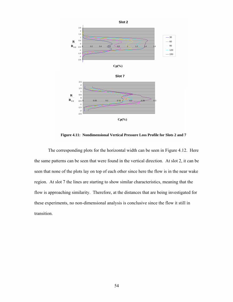
54

Slot 2

-2.5

-2

-1.5

-1

-0.5

0

0.5

1

1.5

2

2.5

0 0.2 0.4 0.6 0.8 1 1.2 1.4 1.6

30

60

90

120

150

1/2RR

Cp(%)

Slot 7

-2.5-2

-1.5-1

-0.50

0.5

11.5

22.5

0 0.05 0.1 0.15 0.2 0.25 0.3

Cp(%)

1/2RR

Figure 4.11: Nondimensional Vertical Pressure Loss Profile for Slots 2 and 7

The corresponding plots for the horizontal width can be seen in Figure 4.12. Here

the same patterns can be seen that were found in the vertical direction. At slot 2, it can be

seen that none of the plots lay on top of each other since here the flow is in the near wake

region. At slot 7 the lines are starting to show similar characteristics, meaning that the

flow is approaching similarity. Therefore, at the distances that are being investigated for

these experiments, no non-dimensional analysis is conclusive since the flow it still in

transition.

55

Slot 7

0

0.05

0.1

0.15

0.2

0.25

0.3

-4 -3 -2 -1 0 1 2 3 4

1/2RR

Cp(%)

Figure 4.12: Nondimensional Horizontal Pressure Loss Profile for Slots 2 and 7

Summary

The flow characteristics for the single wedges have been discussed and analyzed.

It seems that there are two distinct groups that act the same for the different areas

analyzed. These groups are the small angles with the 30° and 60° wedges and the larger

angles with the 90°, 120 and 150° wedges. These two groups show similar

characteristics for wedge width and for maximum total pressure loss. The variable that

has been shown to form these two groups is the aspect ratio since the larger wedges have

more surface area exposed to the oncoming flow. It has also been shown that the

distances tested were still in the transitional region so the wake patterns have not become

Slot 2

0

0.2

0.4

0.6

0.8

1

1.2

1.4

1.6

-4 -3 -2 -1 0 1 2 3 4

306090120150

1/2RR

Cp(%)

56

similar yet. The next sections will discuss the results that were found for combinations of

wedges. It is necessary to see if the wakes act the same way when different wedge angles

are combined.

4.3 Horizontally Aligned Wedge Results

This section will discuss the test results for the combinations of two wedges that

were aligned horizontally. It was necessary to examine whether the various

characteristics found for the single wedges would be applicable to combinations of

wedges. It was also necessary to look at where the two individual wakes merged and

what was the result. For these tests the wedges were spaced 1/4� from each other. It is

likely that the distance between adjacent airfoils in the eventual array will be placed

similar distances apart. Tests were only conducted on the slots 2-5 since after that point

the wakes were found to merge into one larger wake that had little in common with the

individual wakes. The shape of the different contour plots will be discussed with

emphasis placed on when the individual patterns have merged completely. The

maximum pressure drop found with the combinations of wedges will be compared to that

found with the single wedges. Also, the flow pattern for the side-by-side arrangement

will be compared to the single wedge pattern. For the analysis of the wedge

combinations it was not necessary to compare the different arrangements to each other.

This had already been done with the data from the single wedge testing. Instead, the

analysis focused on if the single wedge data gave some indication of what would occur

with combinations of these same wedges.

57

Total Pressure Loss Contours

Contour plots showing how Cp varied across the test section were made for all of

the wedge combinations that were tested in the horizontal alignment tests. The complete

set of these plots can be found in Appendix C. The wake pattern behind horizontal

combinations of wedges is different from single wedges for many reasons. The 3-D

effects will only be seen on the outer edges of the two airfoils. Therefore, the flow

characteristics will not vary as much depending on the aspect ratio. The inside edges are

so close together that the flow doesn�t show as much separation. The two wakes also

combine to form a region of constructive interference that is show by an increased

pressure loss. This region is located between the two wedges and the two peaks of total

pressure loss seen in the single wedge analysis are not as apparent.

Once again a 3-D plot will be shown of one combination of wedges to emphasize

the differences in the pressure loss seen behind the wedge combination. Figure 4.13

shows a 90° wedge next to a 60° wedge with measurements taken at slot 2. Here can be

seen the difference in pressure drop behind the adjacent wedges. At this location, it can

be seen that the two wakes have not really started to merge very much and the

characteristics for the different opening angles is visible. It is also interesting to note the

support rod. The pressure drop caused by this rod is very insignificant with respect to the

pressure drop from the wedges.

58

0

0.5

1Cp(%

)

45

67

8

Distance (inches) 4

5

6

7

8

Distance

(inch

es)

Cp(%)1.51.3751.251.12510.8750.750.6250.50.3750.250.1250

90 Degree and 60 Degree Wedges (side-by-side) - Slot 2

Figure 4.13: 3-D Total Pressure Drop Contour for a 90° and 60° Wedge Aligned Horizontally at Slot 2

All of the combinations of horizontal wedges showed total pressure loss patterns

that were similar to each other. Due to this fact, only one combination of wedges will be

followed downstream and examined in detail here. Other combinations can be viewed in

Appendix C. The contour plots for a combination of a 90° wedge adjacent to a 60°

wedge will be shown at the four downstream distances measured, slots 2-5. For all of

these plots the larger angle wedge is always on the left side. These plots will be

compared to the individual contour plots for the corresponding single wedges. The

individual contour plots were scaled so that the distances line up with the data for the

combination plots. The individual plots were then overlayed to form a plot showing what

the wake shapes would look like if the wakes did not interact. This has not been done for

all of the data since this combination gives a good representation of what occurs.

Figure 4.14 shows the 60° and 90° horizontal combination contour plot at slot 2

along with the overlayed single wedge plots at the same distance. It can be seen that the

shapes of the two wakes are still roughly the same size. The pressure loss has increased

59


4

5

6

7

8

Dis

tanc

e(in

ches

)

Cp(%)1.51.3751.251.12510.8750.750.6250.50.3750.250.1250

Overlay Plot at Slot 2

from that found with the single wedges due to the two wakes interacting with each other.

The maximum pressure loss coefficient has increased 14% from the maximum value

found with the 90° single wedge data. At this distance the peak level of pressure loss is

still behind the larger wedge, but this high Cp region also extends towards the smaller

angle wedge. The two distinct regions of higher pressure loss found with the single

wedge data can be seen only in the 90° side of the combination plot.

Figure 4.14: 60° and 90° Horizontally Aligned Airfoils Total Pressure Drop Contours at Second Slot

Figure 4.15 shows the same plots but the distance has moved to slot 3. At this

slot, the wakes have begun to merge. The size of the individual wakes can still be seen,

but the location of the peak pressure loss has moved. This peak has shifted to the center

between the two wedges. The max pressure loss coefficient has increased by over 50%

from the maximum found in either one of the two individual wedges. The combined

wakes give a greater pressure drop that is not dissipated as rapidly due to the free stream


4

5

6

7

8

Dis

tanc

e(in

ches

)

Cp(%)1.51.3751.251.12510.8750.750.6250.50.3750.250.1250

Combination Plot at Slot 2

60


4

5

6

7

8

Dis

tanc

e(in

ches

)

Cp(%)1.51.3751.251.12510.8750.750.6250.50.3750.250.1250


flow interaction that is found in the single wedges. At this slot it is believed that the two

different angle wakes can still be distinguished.

Figure 4.15: 60° and 90° Horizontally Aligned Airfoils Total Pressure Drop Contours at Third Slot

The contour plots at slot 4 can be seen in Figure 4.16. Here it can be seen that the

combined plot is starting to not show the same characteristics that the single wedge plot

has. In the single wedge contours the 60° wedge wake is nearly the same height as the

90° wedge. However, in the combination plot there is clearly a decrease in wake size

from the larger wedge to the smaller one. It seems that the wake pattern found with the

individual wedge analysis is changed when the wakes interact. The vortices coming off

the top and bottom of the different wedges combine differently to form wake patterns. At

this distance downstream the maximum pressure region is again located between the two

wedges and has increased by nearly 60% over either of the single wedge pressure loss

coefficients. It is also becoming more difficult to visually find where one wake starts and

the next begins due to the mixing that is occurring.


4

5

6

7

8

Dis

tanc

e(in

ches

)

Cp(%)1.51.3751.251.12510.8750.750.6250.50.3750.250.1250


61


4

5

6

7

8

Dis

tanc

e(in

ches

)

Cp(%)1.51.3751.251.12510.8750.750.6250.50.3750.250.1250


Figure 4.16: 60° and 90° Horizontally Aligned Airfoils Total Pressure Drop Contours at

Fourth Slot

The final contour plots for the 60°and 90° wedge horizontal combination for slot

5 can be seen in Figure 4.17. Here it can be seen that the wake for the combination looks

nothing like the individual wakes. The 60° wake pattern was larger when the individual

analysis was done and the 90° wedge wake was much wider in the horizontal direction.

It seems at this distance that the combination wake has very little in common with the

individual wakes. It was expected that the wake on the side of the 90° wedge would have

spread further in the horizontal direction away from the smaller wedge. This was not the

case and this trend also continued for all of the combinations of 120° wedges. The wakes

interact in such a way that the wake is not pushed to the outside. The maximum pressure

loss is also greatly increased over any found with the individual data at these angles. The

pressure loss coefficient increased by over 65%. What was interesting was that the

maximum pressure loss was found in two peaks that were on either side of the support


4

5

6

7

8

Dis

tanc

e(in

ches

)

Cp(%)1.51.3751.251.12510.8750.750.6250.50.3750.250.1250


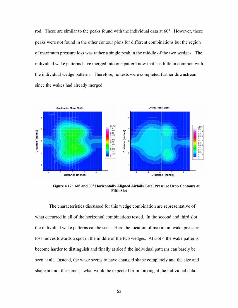
62

rod. These are similar to the peaks found with the individual data at 60°. However, these

peaks were not found in the other contour plots for different combinations but the region

of maximum pressure loss was rather a single peak in the middle of the two wedges. The

individual wake patterns have merged into one pattern now that has little in common with

the individual wedge patterns. Therefore, no tests were completed further downstream

since the wakes had already merged.

Figure 4.17: 60° and 90° Horizontally Aligned Airfoils Total Pressure Drop Contours at

Fifth Slot

The characteristics discussed for this wedge combination are representative of

what occurred in all of the horizontal combinations tested. In the second and third slot

the individual wake patterns can be seen. Here the location of maximum wake pressure

loss moves towards a spot in the middle of the two wedges. At slot 4 the wake patterns

become harder to distinguish and finally at slot 5 the individual patterns can barely be

seen at all. Instead, the wake seems to have changed shape completely and the size and

shape are not the same as what would be expected from looking at the individual data.


4

5

6

7

8

Dis

tanc

e(in

ches

)

Cp(%)1.51.3751.251.12510.8750.750.6250.50.3750.250.1250



4

5

6

7

8

Dis

tanc

e(in

ches

)Cp(%)1.51.3751.251.12510.8750.750.6250.50.3750.250.1250


63

All of the combinations showed an increase in the pressure loss compared to the

individual wedge data. The pressure loss also does not seem to dissipate as much with

two wedges as with one. The pressure drop for all the different combinations tested

aligned horizontally will be discussed in the next section.

Maximum Pressure Loss The maximum pressure drops found with the horizontal alignment were greater

than any found with the single wedge data. This occurred because the two wakes merged

together to form combined regions of high pressure loss far downstream. With one angle

staying the same, the pressure loss was increased for all cases with increase in angle of

the other airfoil. This was not the case in the single wedge flow where low angle wedges

acted differently than high angle wedges. It appears that aspect ratio does not play such

as a significant role when wedges are aligned horizontally. Plots of maximum pressure

drop varying with the distance downstream for all of the different combinations tested

can be seen in Figure 4.18.

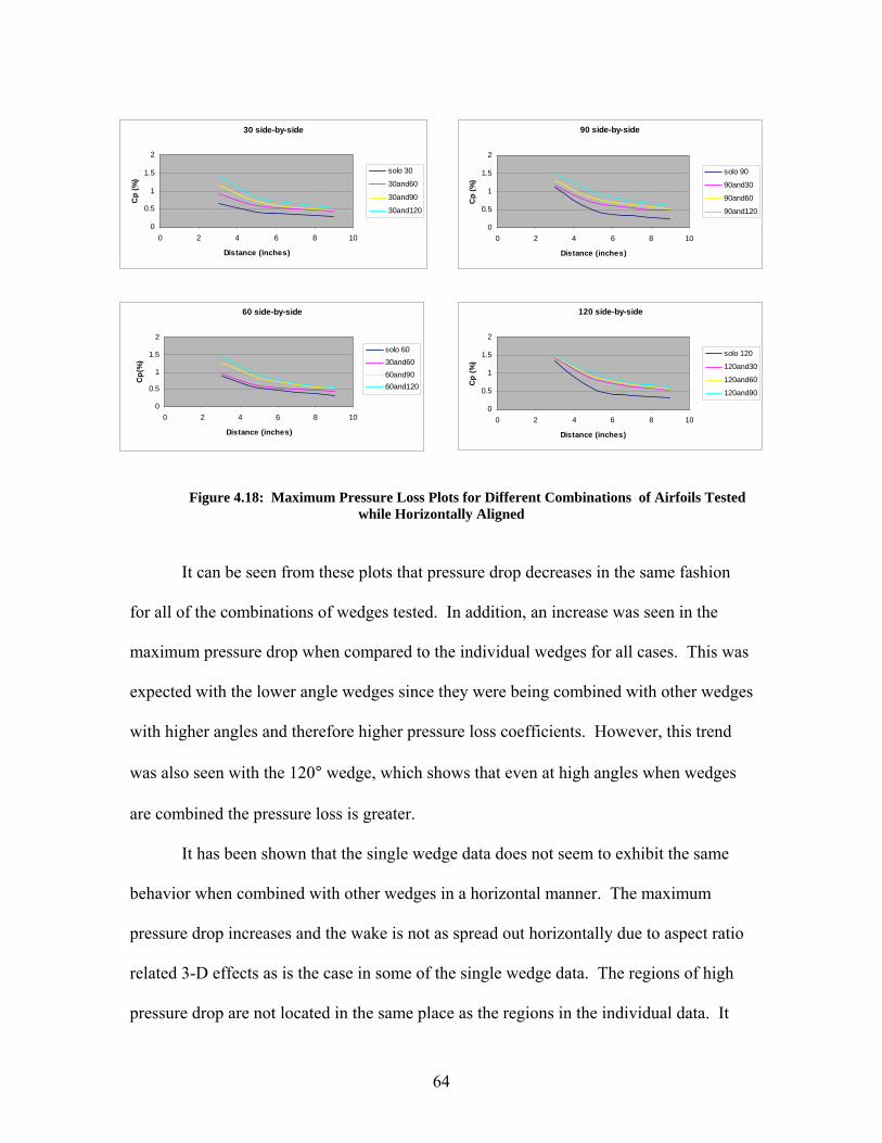
64

Figure 4.18: Maximum Pressure Loss Plots for Different Combinations of Airfoils Tested while Horizontally Aligned

It can be seen from these plots that pressure drop decreases in the same fashion

for all of the combinations of wedges tested. In addition, an increase was seen in the

maximum pressure drop when compared to the individual wedges for all cases. This was

expected with the lower angle wedges since they were being combined with other wedges

with higher angles and therefore higher pressure loss coefficients. However, this trend

was also seen with the 120° wedge, which shows that even at high angles when wedges

are combined the pressure loss is greater.

It has been shown that the single wedge data does not seem to exhibit the same

behavior when combined with other wedges in a horizontal manner. The maximum

pressure drop increases and the wake is not as spread out horizontally due to aspect ratio

related 3-D effects as is the case in some of the single wedge data. The regions of high

pressure drop are not located in the same place as the regions in the individual data. It

90 side-by-side

0

0.5

1

1.5

2

0 2 4 6 8 10

Distance (inches)

Cp

(%)

solo 90

90and30

90and60

90and120

120 side-by-side

0

0.5

1

1.5

2

0 2 4 6 8 10

Distance (inches)

Cp

(%)

solo 120

120and30

120and60

120and90

30 side-by-side

0

0.5

1

1.5

2

0 2 4 6 8 10

Distance (inches)

Cp

(%)

solo 30

30and60

30and90

30and120

60 side-by-side

0

0.5

1

1.5

2

0 2 4 6 8 10

Distance (inches)

Cp(

%)

solo 6030and6060and9060and120

65

useful to see how these regions have shifted to the middle of the wedge combination;

therefore, the next section will discuss this area.

Comparison with Single Wedge Data It has been shown that the horizontally aligned wake patterns differ from those

found in individual wedge analysis. The peak pressure loss region moves to an area

between the two wedges and the maximum pressure drop is increased. This can be seen

directly by comparing the single wedge contour plots to the combination contour plots as

was discussed earlier.

However, an alternative method was also used that just took representative data

for analysis to emphasis the increase and shift in the total pressure loss regions.

To do this for the horizontally aligned wedges, a profile of total pressure loss coefficient

values was taken from the single wedge data. This profile location was taken where the

pressure drop was the greatest and where it was representative of what the flow pattern

looked like at this point. The same profile was taken from the combination data. The

data for the individual wedges was placed with the combination data on one graph. It was

then able to physically see how the wake differed and how the region of higher pressure

loss moved. Figure 4.19 shows an example of where each of the slices was taken for the

three different plots. The comparison being made here is for the same 60°-90° horizontal

alignment arrangement

66

4 5 6 7 83.5

4

4.5

5

5.5

6

6.5

7

7.5

8

90 Degree Single Wedge

Figure 4.19: Typical Profile Locations for Comparison of Wedges for Horizontally Aligned Data

Plots have been made using this slice technique for all of the combinations of

wedges that were tested horizontally. Only the same 60°-90° combination will be

discussed here since all of the wakes show similar characteristics. The complete set of all

the plots can be found in Appendix D.

Figure 4.20 shows the 60°-90° combination at slots 2 and 3. It can be seen at slot

2 that the curves on either side of the combination plot match the single wedge data. The

slope is the same up until the top of each individual curve. It can also be noted that there

is an increase in the total pressure loss coefficient due to the mixing of the two wakes.

This constructive interference is seen with all the combinations aligned horizontally. The

region of highest pressure loss at slot 2 is located behind the 90° wedge. At slot 3 it can

be seen that the individual curves still match the combination curve on the outside. The

maximum pressure loss region is greater than the individual data and the peak is moving

closer to the center between the wedges.

4 5 6 7 83.5

4

4.5

5

5.5

6

6.5

7

7.5

8


4 5 6 7 8

4

5

6

7

8

60 and 90 Degrees Horizontally Aligned

67

Figure 4.20: Comparison of 60° and 90° with Horizontal Alignment to Single Wedge Data at Slots 2 and 3

Figure 4.21 shows the same wedge combination at slots 4 and 5. Here it can be

seen that the combination wake profile shows a curve from one side of the wedges to the

other with a maximum pressure drop in the middle of the two wedges. This shows that

the maximum pressure region has moved to the center between the two wedges. This

region is much higher than either maximum Cp found in the single wedge data. The

individual patterns no longer give a good representation of what is occurring with the

combined wake pattern, but have instead taken on different wake characteristics.

Slot 2

0

0.2

0.4

0.6

0.8

1

1.2

1.4

3 4 5 6 7 8 9

Horizontal Distance (inches)C

p (%

)

60 and 906090

Slot 3

0

0.2

0.4

0.6

0.8

1

1.2

1.4

3 4 5 6 7 8 9

Horizontal Distance (inches)

Cp

(%) 60 and 90

6090

68

Figure 4.21: Comparison of 60° and 90° with Horizontal Alignment to Single Wedge Data at Slots 4 and 5

Summary The horizontal combinations all showed similar characteristics for the different

tests that were completed. The individual wake patterns can really only be seen at the

second and third slot. Further downstream, the wakes combine and form one larger wake

region. There is greater maximum pressure loss found with the combinations than with

the individual data. The regions of higher pressure loss also moved towards the center

between the two wedges. Analyzing the single wedge data does not give a good

representation of what occurs to the wake when wedges are combined horizontally. It

Slot 4

0

0.2

0.4

0.6

0.8

1

1.2

1.4

3 4 5 6 7 8 9


Cp (%

) 60 and 906090

Slot 5

0

0.2

0.4

0.6

0.8

1

1.2

1.4

3 4 5 6 7 8 9


Cp (%

) 60 and 906090

69

does give a decent representation of the size of the wake, but the intensity and the shape

do change as the wakes are combined. In the actual array of these airfoils it might be

desired to change the distortion level quickly in a short distance. This would not be very

possible with the airfoils this close together. The wakes interact too much to have a

difference noted immediately. Therefore, different horizontal distances might be used in

the final array of splitting airfoils.

4.4 Vertically Aligned Wedge Results

This section will discuss the test results for the combinations of two wedges that

were aligned vertically. The same types of analyses that were done on the horizontal

wedges will be applied to the vertical wedges. For these tests the wedges were spaced

with a 1/4� gap between the two airfoils when fully opened. Again, tests were only

conducted at slots 2-5. The shape of the different distortion contour plots will be

discussed with emphasis placed on when and to what extent the individual patterns have

merged. The maximum pressure drop found with the combinations of wedges will be

compared to that found with the single wedges. Also, the flow patterns for the vertical

arrangement will be compared to the single wedge patterns. For this discussion, two

different combinations will be analyzed since they showed different behavior. There will

also be some discussion on trying to predict the patterns that are found using data from

the individual wedges. The data was analyzed to see if the combination wake pattern

could be predicted by superimposing individual wake patterns.

70

Total Pressure Loss Contours

Contour plots showing how Cp varied across the test section were made for all of

the wedge combinations that were tested in the vertical alignment tests. The complete set

of these plots can be found in Appendix E. The wake pattern behind vertical

combinations of wedges is different from single wedges and the horizontal wedge

combinations for many reasons. The separation streamlines coming off of the individual

wedges will intersect each other and cause the flows to merge. This type of arrangement

will also have the eddies formed on the trailing edge interact with each other forming

strong mixing zones. Again, the two wakes will combine to form a region of higher

pressure loss. This region is located in the space between the two wedges and is marked

by a single area of maximum pressure loss. This region also seems to spread in the

horizontal direction as the flow progresses downstream.

A 3-D plot of the 60°-90° wedge combination at slot 2 can be seen in Figure

4.22. In this plot the 90° wedge is the one on the bottom that has the greater pressure

drop. Here the two individual wake patterns can still be seen although there is some

mixing that is occurring. This causes the lower half of the 60° wedge to have a greater

pressure drop than the upper half. The two distinct zones of peak levels of pressure drop

can easily be seen by using this 3-D plot for both of the wedges. The magnitude of the

larger pressure drop caused by the 90° wedge is also clearly visible here.

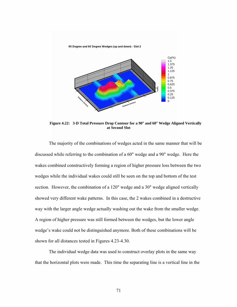
71

0

0.5

1

Cp( %

)4

6

8

Distance (inches)4

6

8

Distance (inches)

Cp(%)1.51.3751.251.12510.8750.750.6250.50.3750.250.1250

90 Degree and 60 Degree Wedges (up and down) - Slot 2

Figure 4.22: 3-D Total Pressure Drop Contour for a 90° and 60° Wedge Aligned Vertically at Second Slot

The majority of the combinations of wedges acted in the same manner that will be

discussed while referring to the combination of a 60° wedge and a 90° wedge. Here the

wakes combined constructively forming a region of higher pressure loss between the two

wedges while the individual wakes could still be seen on the top and bottom of the test

section. However, the combination of a 120° wedge and a 30° wedge aligned vertically

showed very different wake patterns. In this case, the 2 wakes combined in a destructive

way with the larger angle wedge actually washing out the wake from the smaller wedge.

A region of higher pressure was still formed between the wedges, but the lower angle

wedge�s wake could not be distinguished anymore. Both of these combinations will be

shown for all distances tested in Figures 4.23-4.30.

The individual wedge data was used to construct overlay plots in the same way

that the horizontal plots were made. This time the separating line is a vertical line in the

72

center of the two wedges. This was done for both combinations that will be discussed for

all of the distances that were measured. These plots will be used to show how the wake

pattern changes when wedges are combined in a vertical arrangement. For all of the

vertically aligned combination plots, the larger angle is always on the bottom. There will

be shown two different vertically aligned combination plots at all four distances tested.

Figure 4.23 shows the 60° and 90° combined contour plots at slot 2. At this

distance, the two wakes have not really started to merge at all and both patterns can

clearly be seen. The lower half of the 60° wedge is starting to show some mixing so a

larger pressure drop can be noticed there. Most of the combinations tested showed both

individual wake patterns clearly at this distance. The only exception with the

combinations tested was the 90° and 120° vertical arrangement. In that case, the wakes

were so large that mixing occurred immediately. That arrangement was the only one

where the initial patterns could not be seen at this distance.

Figure 4.23: 60° and 90° Vertically Aligned Airfoils Total Pressure Drop Contours at Slot 2


3

4

5

6

7

8

9

Dis

tanc

e(in

ches

)

Cp(%)1.51.3751.251.12510.8750.750.6250.50.3750.250.1250



3

4

5

6

7

8

9

Dis

tanc

e(in

ches

)

Cp(%)1.51.3751.251.12510.8750.750.6250.50.3750.250.1250


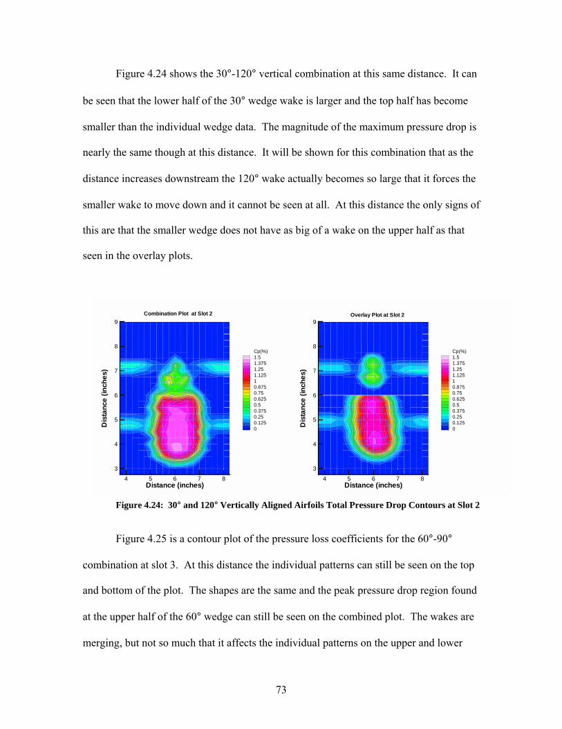
73

Figure 4.24 shows the 30°-120° vertical combination at this same distance. It can

be seen that the lower half of the 30° wedge wake is larger and the top half has become

smaller than the individual wedge data. The magnitude of the maximum pressure drop is

nearly the same though at this distance. It will be shown for this combination that as the

distance increases downstream the 120° wake actually becomes so large that it forces the

smaller wake to move down and it cannot be seen at all. At this distance the only signs of

this are that the smaller wedge does not have as big of a wake on the upper half as that

seen in the overlay plots.


Figure 4.25 is a contour plot of the pressure loss coefficients for the 60°-90°

combination at slot 3. At this distance the individual patterns can still be seen on the top

and bottom of the plot. The shapes are the same and the peak pressure drop region found

at the upper half of the 60° wedge can still be seen on the combined plot. The wakes are

merging, but not so much that it affects the individual patterns on the upper and lower


3

4

5

6

7

8

9

Dis

tanc

e(in

ches

)

Cp(%)1.51.3751.251.12510.8750.750.6250.50.3750.250.1250



3

4

5

6

7

8

9

Dis

tanc

e(in

ches

)

Cp(%)1.51.3751.251.12510.8750.750.6250.50.3750.250.1250


74

portion of the wake. There is an increased pressure loss region that is formed in the

middle between the two wedges. This constructive interference is similar to what was

seen with the horizontally aligned data. The pressure loss coefficient has been increased

by over 40% from any of the individual wedges. The behavior of this combination is

typical of most of the vertical combinations that were tested at this distance.


Figure 4.26 is a contour plot at the same distance for the vertical combination of

30° and 120°. Interesting wake patterns are seen here that differ greatly from the

individual patterns. The 120° wedge on the bottom still has the same shape on the lower

half but the maximum pressure loss has increased by nearly 40% over any of the

individual data. This region is still located directly behind the larger angle wedge. The

top of the 30° wedge wake cannot be seen at all. The flow coming off the larger angle

wedge has interacted in a destructive way with the smaller wedge so that the smaller

wake has been moved down into the 120° wake. The flow that is separating off the


3

4

5

6

7

8

9

Dis

tanc

e(in

ches

)

Cp(%)1.51.3751.251.12510.8750.750.6250.50.3750.250.1250



3

4

5

6

7

8

9

Dis

tanc

e(in

ches

)

Cp(%)1.51.3751.251.12510.8750.750.6250.50.3750.250.1250


75

individual wedges has combined and formed vortices that move behind the 120° wedge

and not behind the smaller angle. This is an interesting result that was not expected from

the individual data. This trend continues downstream until the smaller wake really can�t

be distinguished at all.


The contour plots for the 60°-90° wedge combination at the fourth slot can be

seen in Figure 4.27. Here the individual wake patterns can still be seen on the outer

portions of the larger wake. The two peak areas of maximum pressure loss can even still

be seen on the upper and lower portion of the wake for both of the wedges. The highest

pressure drop is found between the two wedges and here the wake is increasing in size in

the horizontal direction. This region has a pressure loss coefficient that has increased by

over 60% from any of the individual wedge data. At this location the wakes are still

combining in a constructive manner to form a higher pressure drop region.


3

4

5

6

7

8

9

Dis

tanc

e(in

ches

)

Cp(%)1.51.3751.251.12510.8750.750.6250.50.3750.250.1250



3

4

5

6

7

8

9

Dis

tanc

e(in

ches

)

Cp(%)1.51.3751.251.12510.8750.750.6250.50.3750.250.1250


76


The contour plots for the 30°-120° wedge combination for slot 4 can be seen in

Figure 4.28. At this distance, the combination plots show some likeness but also some

major differences from the individual data. The wake shape on the bottom of the 120°

wedge is the same as the one found with the individual data. The region of maximum

pressure loss has shifted slightly and is still located behind the 120° wedge, but has

increased by nearly 50% from the individual data. The 30° wedge wake is what differs

the greatest from the individual data. The wake from this wedge cannot be seen at all

above the support rods. The only way to tell that it is even there is because the changes it

has caused in the wake pattern of the 120° wedge. All of the wake from the top of the

small wedge has been washed out and absorbed by the 120° wedge wake. This is a very

clear example of the type of destructive interference this particular pattern exhibits.


3

4

5

6

7

8

9

Dis

tanc

e(in

ches

)

Cp(%)1.51.3751.251.12510.8750.750.6250.50.3750.250.1250



3

4

5

6

7

8

9

Dis

tanc

e(in

ches

)

Cp(%)1.51.3751.251.12510.8750.750.6250.50.3750.250.1250


77


The contour plot for the 60°-90° vertically aligned wedge combination at slot 5

can be seen in Figure 4.29. Even at this distance the individual wake patterns can still be

seen on the upper and lower portion of the combination plot. Both of these areas are

slightly smaller, but the shape of the wake is still the same. The wakes have combined

and formed a larger wake in the middle between the two wedges and it is about the same

width as the individual 90° wake. This region does have a greater pressure drop and has

a Cp value that is 65% greater than any found for the individual data. The wakes have

effectively mixed at this point and no other tests were run at further distances. This was

because this was the distance where no individual wakes could be seen for the

horizontally aligned tests.


3

4

5

6

7

8

9

Dis

tanc

e(in

ches

)Cp(%)1.51.3751.251.12510.8750.750.6250.50.3750.250.1250



3

4

5

6

7

8

9

Dis

tanc

e(in

ches

)

Cp(%)1.51.3751.251.12510.8750.750.6250.50.3750.250.1250


78


Figure 4.30 shows the 30°-120° wedge combination at slot 5. At this distance, the

individual wakes really don�t have anything in common with the single wedge data. The

120° individual wedge data is much more spread out than the combined plot. The area of

maximum pressure loss is still located behind the upper half of the 120° wedge. This

pressure loss coefficient has a value that is nearly 60% greater than any of the individual

data. Once again, the upper half of the 30° wedge wake cannot be seen at all. This

combination is the only one where this behavior was seen, and it was seen at every slot

tested. This is obviously something that would need to be avoided in an array of these

airfoils. A possibility is just to not have any of the airfoils open to an angle this big when

an array is built. Another solution could be to change the spacing that is found between

adjacent airfoils. With an increase in spacing between the adjacent airfoils, there may not

be as much of this destructive interference.


3

4

5

6

7

8

9

Dis

tanc

e(in

ches

)

Cp(%)1.51.3751.251.12510.8750.750.6250.50.3750.250.1250



3

4

5

6

7

8

9

Dis

tanc

e(in

ches

)

Cp(%)1.51.3751.251.12510.8750.750.6250.50.3750.250.1250


79


It was found during the analysis of the vertically aligned contour plots that the

majority of the combinations acted in a similar way. At the second slot the two distinct

wake patterns could be seen, with little mixing of the two wakes. Further downstream,

the wakes began mixing and a region of higher pressure drop was formed between the

two wedges. This region spread in the horizontal direction and was wider than either of

the two individual patterns. The individual characteristics could still be seen on the top

and bottom of the wake where the two wakes really didn�t mix. For the majority of

combinations, this mixing of the wakes was in a constructive way that gave the higher

pressure drop in the middle. However, for the case of the 30°-120° combination the two

wakes combined in a destructive way. The 120° wake completely washed out the smaller

wake and no individual wake patterns were seen here except at the second slot. There

was still a region of higher pressure loss, but this region was located behind the 120°

wedge at all locations. This destructive interference should be avoided when an actual

array of airfoils is built. Therefore, the 1/4� distance between the two airfoils might need


3

4

5

6

7

8

9

Dis

tanc

e(in

ches

)Cp(%)1.51.3751.251.12510.8750.750.6250.50.3750.250.1250



3

4

5

6

7

8

9

Dis

tanc

e(in

ches

)

Cp(%)1.51.3751.251.12510.8750.750.6250.50.3750.250.1250


80

to be increased so this does not occur. Another option would be to not have any of the

airfoils open to angles this large to avoid this behavior

Maximum Pressure Loss It was shown in the contour plots that the two individual wakes combined to form

a region of higher pressure drop. This region was located between the two wedges for

the majority of the combinations tested with the vertical alignment. These regions were

marked by an increase in pressure loss coefficient compared to the individual wedge data.

The plots of maximum pressure drop varying with the distance downstream can be seen

for all of the combinations tested in Figure 4.31.

Figure 4.31: Maximum Pressure Loss Plots for Different Combinations of Airfoils Tested

while Vertically Aligned

30 Up and Down

0

0.5

1

1.5

0 2 4 6 8 10

Distance (inches)

Max

Cp

(%) solo 30

30and60

30and90

30and120

60 Up and Down

00.20.40.60.8

11.21.4

0 2 4 6 8 10

Distance (inches)

Max

Cp

(%) solo 60

30and60

60and90

60and120

90 Up and Down

00.20.40.60.8

11.21.4

0 2 4 6 8 10

Distance (inches)

Max

Cp

(%) solo 90

90and30

90and60

90and120

120 Up and Down

0

0.5

1

1.5

0 2 4 6 8 10

Distance (inches)

Max

Cp

(%) solo 120

120and30

120and60

120and90

81

The general trends shown in these plots are that the individual data had the

smallest pressure loss, and when combined with other wedges in a vertical fashion the

pressure loss increased as the angle increased. With the 90° and 120° there was some

variation from this trend at the second slot. However, these differences were really not

very large compared to the change from the individual data. These plots show that when

combined in a vertical fashion, the wedges exhibit behavior that would be expected at

these distances with the pressure loss increasing with increasing angle. This was not

always the case with the individual data and this shows that combining wedges gives a

more consistent pressure drop. The individual wakes are not representative of what

occurs with combined wakes since the pressure drop increases and shifts position. This

shifting of the position of highest pressure drop will be discussed next.

Comparison with Single Wedge Data It has been shown that combining wedges in a vertical alignment produces a

higher maximum pressure drop than with either individual wedge. For most of the cases

this region is centered between the two wedges and marks the location where the wakes

have combined the most. This trend can be seen directly by comparing the individual

contour plots to the combination contour plots to examine how the regions have shifted.

For the vertically aligned combinations, a profile of the wake pressure drop taken directly

down the center of the two wakes can show the important characteristics of each wake.

This shows how the pressure loss coefficient varies across the test section and is a better

indication of how much the maximum pressure drop region has shifted. A vertical profile

was taken from each of the individual contour plots at the location in the middle of the

82

4 5 6 7 83.5

4

4.5

5

5.5

6

6.5

7

7.5

8


wake behind each wedge. These profiles were combined with the profile that was taken

from the same location in the combined contour plots. These plots are capable of

showing how the region of maximum pressure drop moves. Figure 4.32 shows an

example where each of the profiles were taken for the three different plots. The

combination here is the 60°-90° vertical alignment at slot 2.

Figure 4.32: Typical Profile Locations for Comparison of Wedges for Horizontally Aligned Data

Plots have been made using this technique described for all of the wedges that

were tested vertically. The entire set of these plots for vertical combinations at all

distances that were tested can be found in Appendix F. The 60°-90° vertical arrangement

showed typical behavior for all of the combinations. Therefore, this combination will be

shown using the technique described above. In addition the 30°-120° wedge combination

will also be discussed again to show how the smaller wedge wake was completely

engulfed by the larger wake.

4 5 6 7 83.5

4

4.5

5

5.5

6

6.5

7

7.5

8


4 5 6 7 83

4

5

6

7

8

960 and 90 Degrees Vertically Aligned

83

Figure 4.33 shows the 60°-90° wedge combination aligned vertically at slots 2

and 5. These two plots show how the wake pattern and maximum pressure drop change

as the distance is increased downstream as compared to the single wedge data. At slot 2

it can be seen that the curves are nearly the same as those seen with the single wedge

data. This was also apparent in the plots of this type that were made for the horizontal

alignment. At this distance the wakes have not combined yet. At slot 5, it can be seen

that constructive interference is occurring and the maximum pressure drop region has

moved to the point between the two wedges. This region shows a higher pressure drop

than either seen for the individual analysis. The individual wakes on the upper and lower

portion can still be seen on the combined curve and the intensity of this pressure drop is

nearly the same on the outer edges of the wake. These plots are representative of what

happened with most of the vertical combinations tested.

84

Figure 4.33: Comparison of 60° and 90° with Vertical Alignment to Single Wedge Data at Slots 2 and 5

Figure 4.34 shows the comparison of the 30°-120° combination aligned vertically

at slots 2 and 5. It can be seen at slot 2 that the individual curves are almost identical to

the one seen with the combination of the two wedges. There is little mixing that has

occurred since the distance is so close behind the wedge. Here both of the individual

peaks of pressure drop can still be seen for the two wedges. At this distance, this

combination acts just like all of the other ones that were tested. At slot 5 it can be seen

that the smaller wedge wake has been completely moved. The 120° wedge wake has

become much larger and has absorbed the wake seen from the 30° wedge. This

combination was the only one that showed this characteristic for the vertically aligned

wedges. There was destructive interference seen with this combination since the larger

Slot 2

2

3

4

5

6

7

8

9

0 0.2 0.4 0.6 0.8 1 1.2

Cp (%)

Vert

ical

Dis

tanc

e (in

ches

)

60 and 906090

slot 5

2

3

4

5

6

7

8

9

0 0.2 0.4 0.6 0.8 1 1.2

Cp (%)

Vert

ical

Dis

tanc

e (in

ches

)

60 and 906090

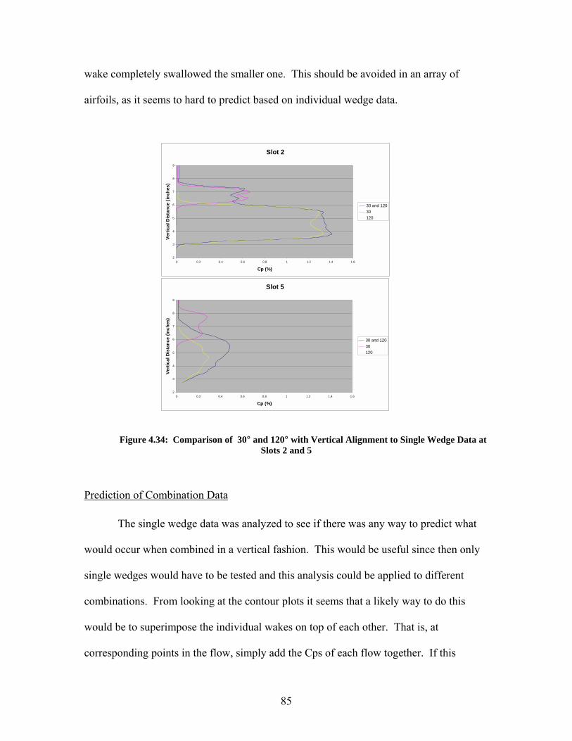
85

wake completely swallowed the smaller one. This should be avoided in an array of

airfoils, as it seems to hard to predict based on individual wedge data.

Figure 4.34: Comparison of 30° and 120° with Vertical Alignment to Single Wedge Data at Slots 2 and 5

Prediction of Combination Data The single wedge data was analyzed to see if there was any way to predict what

would occur when combined in a vertical fashion. This would be useful since then only

single wedges would have to be tested and this analysis could be applied to different

combinations. From looking at the contour plots it seems that a likely way to do this

would be to superimpose the individual wakes on top of each other. That is, at

corresponding points in the flow, simply add the Cps of each flow together. If this

Slot 2

2

3

4

5

6

7

8

9

0 0.2 0.4 0.6 0.8 1 1.2 1.4 1.6

Cp (%)

Vert

ical

Dis

tanc

e (in

ches

)

30 and 12030120

Slot 5

2

3

4

5

6

7

8

9

0 0.2 0.4 0.6 0.8 1 1.2 1.4 1.6

Cp (%)

Vert

ical

Dis

tanc

e (in

ches

)

30 and 12030120

86

method shows that it can predict the combined wakes, then it would be very easy to see

what would occur with combinations aligned vertically by using the individual data and

could probably be applied to combinations of more than two wedges. This was done for

many of the combinations of vertically aligned data with mixed results.

Figure 4.35 shows the two individual wakes superimposed on top of each other

for the 60°-90° combination at slot 4, along with the actual contour plot at slot 4. The

general trends that were found with this method can be seen in this graph. The method

was good at slots 3-5 for predicting the maximum pressure loss coefficient and the

location where it would be located. This can be seen in the contour plot since the peak

zones are of the same intensity and located at the same location on both of the plots.

However, this method was not very successful at predicting the shape of the combined

wake, especially how the wake would spread in the horizontal direction between the two

wedges. The superimposed wake is not as wide in the horizontal direction as the actual

wake. This method is good for a first approximation of what would happen to the

maximum pressure loss coefficient and where it would occur when the wakes were

combined at slots 3-5. This method did not work well at slot 2 due to the fact that the

wakes had not really begun to mix at this point. For all of the patterns except the 30°-

120° this method worked well for predicting the maximum pressure drop coefficient and

its' location.

87

Figure 4.35: Superimposed and Original Contour Plots for a Combination of 60° and 90° Wedges at Slot 4

To more clearly show how close this prediction was for this data, a profile has

been taken from the superimposed contour plot in the same manner as was discussed in

the previous section. This curve was placed on the same graph as the combination and

individual data so that it could be seen how close the prediction was for the combined

pressure loss coefficient. This plot for the 60°-90° data at slot 4 can be seen in Figure

4.36. It can be seen here that the peaks are nearly in the same location and are of a very

similar magnitude. It was found that this method worked for many of the combinations

that were tested and functions well as a first approximation to what may occur with

vertically combined wedges. This method is not perfect and more tests need to be run on

different combinations of parameters to see when this method would be more successful

for predicting the actual wake pattern that will be formed when combining airfoils at

arbitrary angles.

4 5 6 7 83

4

5

6

7

8

9

Cp(%)1.51.3751.251.12510.8750.750.6250.50.3750.250.1250

Vertically Aligned Combination at Slot 4

4 5 6 7 83

4

5

6

7

8

9

Cp(%)1.51.3751.251.12510.8750.750.6250.50.3750.250.1250

Superimposed Combination at Slot 4

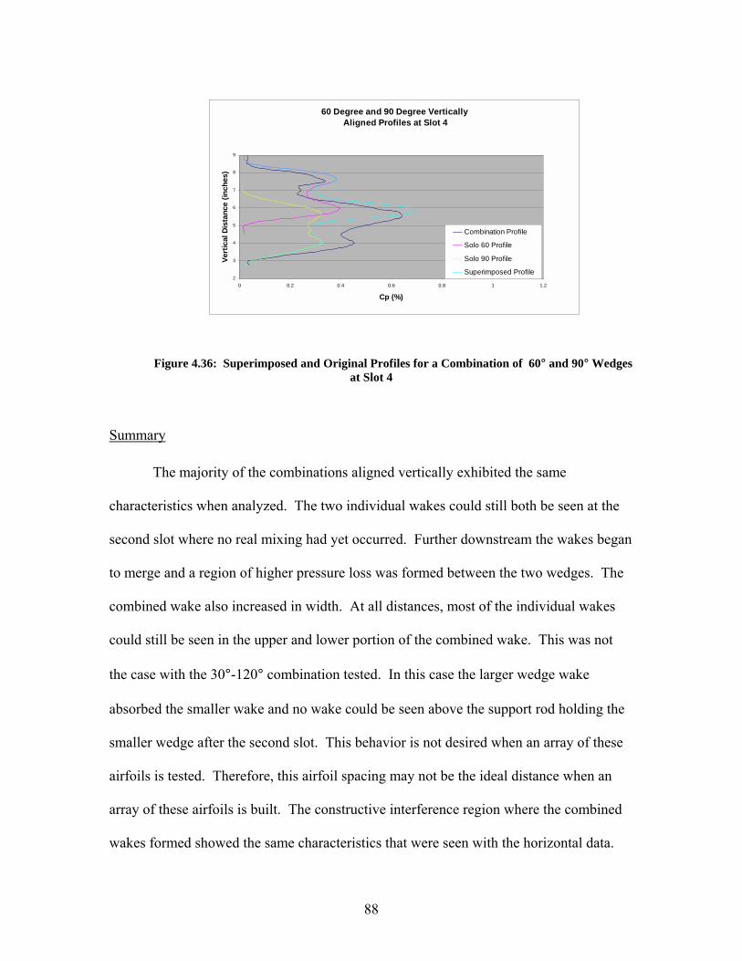
88

Figure 4.36: Superimposed and Original Profiles for a Combination of 60° and 90° Wedges at Slot 4

Summary

The majority of the combinations aligned vertically exhibited the same

characteristics when analyzed. The two individual wakes could still both be seen at the

second slot where no real mixing had yet occurred. Further downstream the wakes began

to merge and a region of higher pressure loss was formed between the two wedges. The

combined wake also increased in width. At all distances, most of the individual wakes

could still be seen in the upper and lower portion of the combined wake. This was not

the case with the 30°-120° combination tested. In this case the larger wedge wake

absorbed the smaller wake and no wake could be seen above the support rod holding the

smaller wedge after the second slot. This behavior is not desired when an array of these

airfoils is tested. Therefore, this airfoil spacing may not be the ideal distance when an

array of these airfoils is built. The constructive interference region where the combined

wakes formed showed the same characteristics that were seen with the horizontal data.

60 Degree and 90 Degree Vertically Aligned Profiles at Slot 4

2

3

4

5

6

7

8

9

0 0.2 0.4 0.6 0.8 1 1.2

Cp (%)

Vert

ical

Dis

tanc

e (in

ches

)Combination Profile

Solo 60 Profile

Solo 90 Profile

Superimposed Profile

89

With few exceptions, the maximum pressure loss was increased with an increase in

opening angle for a constant angle second wedge.

It was also found that superimposing the individual plots often gives a good first

approximation of how the pressure drop will increase when wedges are combined in a

vertical alignment. This method is not capable of predicting what the actual shape of the

wake will look like, but only the location and magnitude of the pressure drop increase. It

is not easy to predict what the actual wake pattern will look like and more testing might

be needed before this can be accomplished.

90

5 Conclusions and Recommendations

Gas turbine engine manufacturers recognize the need for testing aircraft engine

response to inlet distortion. Testing engines for inlet distortion response has been done

for many years to avoid performance problems such as surge that can occur when the

engine does not receive the expected uniform airflow. The unsteady inlet flow can be

caused by total temperature distortion or total pressure distortion. There are different

ways that engine manufacturers test their engines for total pressure distortion including

airjets and screens. These methods are capable of producing steady-state distortion

patterns that can be tested on engines to see what effect the distortion has. Modern

military aircraft are capable of very advanced maneuvers that can introduce transient or

time dependent distortion. The current methods are not able to reproduce this transient

distortion so alternative methods are being investigated that would be able to satisfy these

needs.

One alternative distortion generator that has been studied is the splitting airfoil

concept, which is essentially a wedge that can be opened to different angles. This device

would be one part of an array of splitting airfoils that would replace the airjet or

distortion screen in distortion testing. Each airfoil would be individually controlled,

enabling the user to specify whatever pattern might be needed. This array of airfoils

would be capable of producing steady state distortion and could also introduce transient

distortion by changing the opening angle of the blades. The effects of this distortion

could be studied on the engine to avoid performance problems encountered when

transient behavior is seen in flight.

91

A splitting airfoil design has been built that is capable of being set at different

angles. This design is representative of a splitting airfoil that would be used in an actual

array. Steady-state tests were conducted on this airfoil in an attempt to classify the wake

characteristics. The wake area being examined was from near the wedge trailing edge to

thirteen inches downstream of the airfoil. Tests were run on single airfoils at different

opening angles and on combinations of airfoils that were aligned both vertically and

horizontally. The total pressure was measured at several planes downstream of the

airfoil.

5.1 Conclusions

The single wedge data showed some interesting characteristics. The wake

characteristics were separated into two groups depending on their aspect ratio. Here the

aspect ratio is the ratio of the width of the airfoil over the distance between trailing edges.

The first group with an aspect ratio less than one consisted of the airfoils with the 30° and

60° opening angle. The other group with an aspect ratio greater than one consisted of

wedges with opening angles of 90°, 120°, and 150°. The reason that the aspect ratio was

so important is because at higher angles there is more frontal surface area exposed to the

flow and the flow separates on the sides of the airfoils instead of just on the trailing

edges. This flow separation on the sides of the wedge makes the two groups of airfoils

act in different ways.

For the group with the aspect ratio less than one, it was found that the wake shape

was similar at all distances downstream. This wake shape was characterized by two

92

regions of peak total pressure drop that were found above and below the support strut. In

addition, these wedge angles exhibited more 2-D behavior by the wake spreading in the

vertical direction much more than the horizontal direction. The wake width was larger

for the 60° wedge than for the 30° at all downstream distances. For this group it was also

found that the maximum pressure drop was greater for the larger angle wedge at all

distances.

The group of airfoils with the aspect ratio greater than one had similar

characteristics to the other group at the first few slots tested. Here the wake was larger in

the vertical direction than the horizontal direction. At farther distances downstream, the

wake spread more in the horizontal direction than the vertical direction. This axis

switching was caused by the greater aspect ratio. This wake pattern had two lobes of

higher pressure drop that were formed towards the outside of the wake in the horizontal

direction. At the highest angle tested these lobes had formed into one area of peak

pressure loss extending across the entire wake pattern in the horizontal direction. The

equivalent wake width was nearly the same for this group and the actual width was larger

in the horizontal direction than the vertical direction. This group also showed higher

pressure loss coefficients as the opening angle was increased. When the opening angles

were not classified in these two groups, the maximum pressure loss coefficients did not

increase at all distances as the opening angle was increased. The maximum pressure

coefficient increasing with angle in all cases only occurred at the second and last slot.

A scaling analysis was done on the wake patterns in order to find any similarity

between the different angles at the increasing distances. It was found that at three inches

behind the airfoils the wake was in the near wake region and was dominated by the shape

93

of the bluff body. At the final slot, 13 inches behind the airfoil, the wake was still in the

transitional region, but was approaching the similarity region since the non-dimensional

wake profiles were starting to lay on top of each other. Therefore, none of the scaling

analysis was conclusive since the flow had not reached the similarity region and was still

in transition.

Combinations of airfoils were tested that were aligned in the horizontal direction

with emphasis on whether the individual analysis could be applied to groups of airfoils.

It was found that there were many differences between the characteristics of individual

wedges and those aligned vertically. All of these combinations of airfoils did show wake

characteristics that were the alike when compared to each other.

At a distance of three inches (slot 2) behind the airfoils, the distinct individual

wake patterns could each be seen since this area was greatly influenced by the shape of

the bluff bodies and not much mixing of the wakes had occurred. At five inches (slot 3)

behind the airfoil and continuing downstream the two wakes combined constructively to

form a region of higher pressure loss between the two wedges. In all cases the pressure

drop found in this region was higher than any found with the individual wedges at those

angles. In addition, if one angle remained fixed, the maximum pressure loss coefficient

increased as the adjacent angle was increased. The maximum pressure drop did not

depend on the aspect ratio as seen in the individual analysis. High aspect ratio wedge

effects are not as big of a problem with wedges aligned horizontally because the flow

does not separate on the sides where the two wedges are nearest.

At the final slot measured, nine inches behind the airfoil, the individual wake

patterns had completely merged and none of the individual characteristics could be seen.

94

The constructive interference had created a wake region that usually could not be

predicted from the individual data. In a full array of airfoils, it might be useful to provide

a large cross-stream gradient of the steady-state distortion level over a short distance.

This would not be possible with the spacing between airfoils that was used in these tests.

The wakes combine rapidly so that there really is not a great change in the wake pattern

from the larger to the smaller wedge. If distortion gradients need to be changed over a

short distance, then the airfoils should probably be placed further apart. More

investigation needs to be done with varying the spacing between the airfoils to see how

this variable will affect how the wakes merge.

Combinations of airfoils were also tested that were aligned in the vertical

direction. The majority of the different angle combinations that were tested showed

related characteristics. These characteristics include a constructive wake interference

region that was formed between the two wedges and was marked by a peak level of

pressure loss. This region had greater pressure loss than seen in either of the individual

wedges in the combinations. This region also extended farther in the horizontal direction.

The individual wake shapes could still be seen at the upper and lower part of the

combined wake for most of the test cases. This was not the case for the 30°-120° wedge

combination where the smaller angle wake was completely engulfed the larger one. This

destructive behavior should be avoided when an array of these airfoils is constructed.

Larger spacing between adjacent airfoils needs to be investigated to see if this change

will eliminate the destructive interference that was found here. Another option might be

to only have the splitting airfoils opened to 90° or less. This option would eliminate the

95

destructive interference also. More testing needs to be done to analyze which of these

ideas is viable solution to this problem.

Superimposing the individual wake patterns on top of each other gave a decent

first approximation to how the maximum pressure loss coefficient increases for the

vertical combinations. This method gave close approximations to the maximum pressure

loss and was able to show where this region would be located for many of the

combinations tested. For other combinations, this method did not work well at all. There

was no definite pattern that this trend followed. Also, this method was not a good

approximation for the shape of the combined wake since it did not account for the wake

spreading in the horizontal direction. This method could not be applied to the

horizontally aligned data since it gave no consistent results. Possibly the superimposed

data would show better results with an increase in distance between horizontal wedges.

More testing is needed to collect data to try to identify the reason why this seems to work

for some combinations and not for others. This study would be very useful to be able to

predict the wake patterns in an array from the individual data.

The analysis that has been completed shows that the wake characteristics change

when different wedge angles are combined. The pressure loss is increased and the

maximum pressure loss region shifts position. Trying to use the individual data to predict

the wake pattern that will be produced with different combinations through superposition

is often not very effective. When a full array of these airfoils is eventually constructed,

the wedge wakes will not only be interacting in just the horizontal direction or the

vertical direction. Instead, the wakes will be interacting with each other on all sides and

the patterns will greatly differ from any found with the individual data. These arrays will

96

create wake patterns that will be very difficult to predict without extensive testing.

Combinations of more than two airfoils need to be tested to see how the wakes form

when interacting with the individual wakes in all directions.

5.2 Recommendations

There are many aspects that still need to be investigated before splitting airfoils

can be used effectively in distortion testing. The most important area to research is the

actual actuation mechanism for the splitting airfoil. If mounted on the airfoil, the

actuation device would have to be quite small with little increase in distortion level. The

actuator would also have to be able to change the opening angle from fully closed to

whichever angle was specified very quickly, in order to properly reproduce the desired

transient behavior. The Virginia Tech Turbolab is currently researching actuation

mechanisms for such a device in conjunction with the AEDC. There are several

actuation methods that are being investigated to find the most suitable one.

The characteristics of the splitting airfoil that were analyzed in this report also

need more examination. Different airfoil spacings need to be tested to see what effect

this has on the merging of the wakes. There were many things unfavorable things

discovered in the analysis that may be avoided or minimized by changing this parameter.

The merging of the wakes so close behind the airfoil and the destructive interference that

was seen may be avoided by varying the distance between airfoils. It might be that none

of the airfoils will ever be open to 120°, which would also eliminate this destructive

97

interference. More testing needs to be done to see how these changes affect the wake

pattern.

It is also necessary to examine arrays of airfoils that consist of combinations of

more than two wedges. It has been shown that the wake characteristics change when

different wedge combinations are aligned vertically or horizontally. It is not know what

the wake pattern will look like when more than two of the airfoils interact. The next

testing that should be completed should be an array of four or nine airfoils to see what

patterns are formed.

Standard distortion testing methods used in industry usually produce up to 30%

total pressure drop. The maximum pressure drop that was found with the analysis that

was discussed here was only around 1.5%. This is most likely due to the fact that the

Reynolds number is lower for the tests that were completed than that which will be found

in the actual direct-connect testing. The Reynolds number in these tests was around

74,000 while Reynolds number up to 800,000 will be encountered in the direct-connect

tests. This pressure drop was the greatest that could be created with the facilities that

were available for testing. It is necessary to test some of these combinations of airfoils at

higher Reynolds number in a wind tunnel with higher velocities to see if the wake

patterns that were found would be applicable to the conditions that will be found in the

direct-connect distortion testing. In addition, the devices currently used to produce total

pressure distortion are usually located at least one engine diameter upstream. It was

found with the horizontal combination data that the wake patterns were fully merged at

only 13 inches behind the airfoil. This is a much smaller distance than is currently used

98

in distortion testing. Therefore, tests need to be run so see if the distance where the

individual wake patterns would be merged is the same for higher velocity flow.

The final step before building an array of the splitting airfoils would be to test

them to see what transient effects can be seen. A high-speed data acquisition system

would be needed to accomplish this task. One alternative that may need investigation is a

combination of splitting airfoils and distortion screens. The distortion screens are already

capable of creating the steady-state total pressure distortion patterns that are typical in

everyday flight. If the array of splitting airfoils was placed in front of the distortion

screen then they would cause little disturbance when in the fully closed position. The

opening angles could then be changed quickly to produce rapid changes in distortion

level. The array of airfoils could also be used alone to create steady-state or transient

distortion. Regardless of which method is used, there is still much research that needs to

be done before the splitting airfoil concept will see widespread use in transient total

pressure distortion testing in gas turbine engines.

99

References [1] Biesiadny, T.J., Braithwaite, W.M., Soeder, R.H., and Abdelwahab M., �Summary of Investigations of Engine Response to Distorted Inlet Conditions,� AGARD Conference Proceedings No. 400, September 1986, pp. 15.1-15.20.

[2] Davis, M., Hale, A., and Beale, D., �An Argument for Enhancement of the Current Inlet Distortion Ground Test Practice for Aircraft Gas Turbine Engines,� to be presented at the ASME Turbo Expo 2001, New Orleans Louisiana. [3] SAE Aerospace Recommended Practice, ARP-1420,�Gas Turbine Inlet Flow Distortion Guidelines,� March 1978. [4] SAE Aerospace Information Report, AIR-1419, �Inlet Total-Pressure Distortion Considerations for Gas Turbine Engines,� May 1983. [5] Lawless, P.B., Fleeter, S., �Effect of Controlled Inlet Distortions on Rotating Stall Inception in a Low Speed Centrifugal Compressor,� AIAA Paper No. 94-2799, June 1994.

[6] Beale, D.K., �Simulation Requirement for the Transient Total Pressure Distortion Generator Development,� private correspondence, 1997.

[7] Bruns, J. E., Smith, C. F., �Installed F/A-18 Inlet Flow Calculations at a High Angle of Attack,� Journal of Propulsion and Power Vol. 10, Jan-Feb 1994, pgs. 109-115.

[8] Walsh, K.R., Yuhas, A.J., Williams, J.G., and Steenken, W.G., �Inlet Distortion for an F/A-18A Aircraft During Steady Aerodynamic Conditions up to 60° Angle of Attack,�

NASA Technical Memorandum No. 104329, 1997.

[9] Leinhos, D.C., Schmid, N.R., Fottner, L, �The Influence of Transient Inlet Distortions on the Instability Inception of a Low Pressure Compressor in a Turbofan Engine,� ASME Turbo Expo 2000, Munich, Germany.

[10] DiPietro, T., �Fundamental Wind Tunnel Experiments for Total Pressure Distortion Generator Concept Selection,� Year End Report for Sverdrup Technology, January, 1996.

[11] Jumel, J, King, P.S., O�Brien, W.F., �Transient Total Pressure Distortion Generator Development, Phase II,� Final Report for Academic Qualification, Blacksburg, VA, July, 1999.

[12] http://www.mcmastercarr.com [13] Blevins, R.D., Applied Fluid Dynamics Handbook, Van Nostrand Reinhold Company, 1984, pp. 279-381.

100

[14] Mott, R.L., Machine Elements in Mechanical Design, 2nd Edition, Prentice Hall, 1992, pp. A23-A27. [15] Tkacik, P.T., �Cascade Performance of Double Circular Arc Compressible at High Angle of Attack,� M.S. Thesis in Mechanical Engineering, Virginia Polytechnic and State University, May 1982. [16] Schetz, J.A., Foundations of Boundary Layer Theory for Momentum, Heat and Mass Transfer, Prentice Hall, 1984, pp. 220-254. [17] Yang, J., Tsai, G., and Wang, W., �Near-Wake Characteristics of Various V-Shaped Bluff Bodies,� Journal of Propulsion and Power Vol. 10, Jan-Feb 1994, pp. 47-55. [18] Goldstein, S., Modern Developments in Fluid Dynamics Volume II, Dover Publications, 1965, pp. 550-600. [19] Mutter, T.B., �Numerical Simulations of Elliptical Jets: A Study of Entrainment,� M.S. Thesis in Mechanical Engineering, Virginia Polytechnic and State University, March 1994.

101

Appendix A-Wind Tunnel and Test Section Setup

102

Figure A1: Drawing of Wind Tunnel and Test Section

103

Pictures of Test Setup:

Figure A2: Right Side View of Test Section

Figure A3: Left Side View of Test Section

104

Pictures of Test Setup:

Figure A4: Second Left Side View of Test Section

Figure A5: View of Seven Slots on Test Section

105

Appendix B - Percent Total Pressure Drop Contour Plots for Single Wedges

106

30 degree angle wedge:

Figure B1: Single 30 Degree Wedge Total Pressure Drop Contours


3.5

4

4.5

5

5.5

6

6.5

7

7.5

8

Dis

tanc

e(in

ches

)

Cp(%)1.51.3751.251.12510.8750.750.6250.50.3750.250.1250

Slot 2


3.5

4

4.5

5

5.5

6

6.5

7

7.5

8

Dis

tanc

e(in

ches

)

Cp(%)1.51.3751.251.12510.8750.750.6250.50.3750.250.1250

Slot 3


3.5

4

4.5

5

5.5

6

6.5

7

7.5

8

Dis

tanc

e(in

ches

)

Cp(%)1.51.3751.251.12510.8750.750.6250.50.3750.250.1250

Slot 4


3.5

4

4.5

5

5.5

6

6.5

7

7.5

8

Dis

tanc

e(in

ches

)

Cp(%)1.51.3751.251.12510.8750.750.6250.50.3750.250.1250

Slot 5


3.5

4

4.5

5

5.5

6

6.5

7

7.5

8

Dis

tanc

e(in

ches

)Cp(%)1.51.3751.251.12510.8750.750.6250.50.3750.250.1250

Slot 6


3.5

4

4.5

5

5.5

6

6.5

7

7.5

8

Dis

tanc

e(in

ches

)

Cp(%)1.51.3751.251.12510.8750.750.6250.50.3750.250.1250

Slot7

107




3.5

4

4.5

5

5.5

6

6.5

7

7.5

8

Dis

tanc

e(in

ches

)

Cp(%)1.51.3751.251.12510.8750.750.6250.50.3750.250.1250

Slot 2


3.5

4

4.5

5

5.5

6

6.5

7

7.5

8

Dis

tanc

e(in

ches

)

Cp(%)1.51.3751.251.12510.8750.750.6250.50.3750.250.1250

Slot 3


3.5

4

4.5

5

5.5

6

6.5

7

7.5

8

Dis

tanc

e(in

ches

)

Cp(%)1.51.3751.251.12510.8750.750.6250.50.3750.250.1250

Slot 4


3.5

4

4.5

5

5.5

6

6.5

7

7.5

8

Dis

tanc

e(in

ches

)

Cp(%)1.51.3751.251.12510.8750.750.6250.50.3750.250.1250

Slot 5


3.5

4

4.5

5

5.5

6

6.5

7

7.5

8

Dis

tanc

e(in

ches

)

Cp(%)1.51.3751.251.12510.8750.750.6250.50.3750.250.1250

Slot 6


3.5

4

4.5

5

5.5

6

6.5

7

7.5

8

Dis

tanc

e(in

ches

)

Cp(%)1.51.3751.251.12510.8750.750.6250.50.3750.250.1250

Slot 7

108




3.5

4

4.5

5

5.5

6

6.5

7

7.5

8

Dis

tanc

e(in

ches

)

Cp(%)1.51.3751.251.12510.8750.750.6250.50.3750.250.1250

Slot 2


3.5

4

4.5

5

5.5

6

6.5

7

7.5

8

Dis

tanc

e(in

ches

)

Cp(%)1.51.3751.251.12510.8750.750.6250.50.3750.250.1250

Slot 3


3.5

4

4.5

5

5.5

6

6.5

7

7.5

8

Dis

tanc

e(in

ches

)

Cp(%)1.51.3751.251.12510.8750.750.6250.50.3750.250.1250

Slot 4


3.5

4

4.5

5

5.5

6

6.5

7

7.5

8

Dis

tanc

e(in

ches

)

Cp(%)1.51.3751.251.12510.8750.750.6250.50.3750.250.1250

Slot 5


3.5

4

4.5

5

5.5

6

6.5

7

7.5

8

Dis

tanc

e(in

ches

)Cp(%)1.51.3751.251.12510.8750.750.6250.50.3750.250.1250

Slot 6


3.5

4

4.5

5

5.5

6

6.5

7

7.5

8

Dis

tanc

e(in

ches

)

Cp(%)1.51.3751.251.12510.8750.750.6250.50.3750.250.1250

Slot 7

109




3.5

4

4.5

5

5.5

6

6.5

7

7.5

8

Dis

tanc

e(in

ches

)

Cp(%)1.51.3751.251.12510.8750.750.6250.50.3750.250.1250

Slot 3


3.5

4

4.5

5

5.5

6

6.5

7

7.5

8

Dis

tanc

e(in

ches

)

Cp(%)1.51.3751.251.12510.8750.750.6250.50.3750.250.1250

Slot 2


3.5

4

4.5

5

5.5

6

6.5

7

7.5

8

Dis

tanc

e(in

ches

)

Cp(%)1.51.3751.251.12510.8750.750.6250.50.3750.250.1250

Slot 4


3.5

4

4.5

5

5.5

6

6.5

7

7.5

8

Dis

tanc

e(in

ches

)

Cp(%)1.51.3751.251.12510.8750.750.6250.50.3750.250.1250

Slot 5


3.5

4

4.5

5

5.5

6

6.5

7

7.5

8

Dis

tanc

e(in

ches

)Cp(%)1.51.3751.251.12510.8750.750.6250.50.3750.250.1250

Slot 6


3.5

4

4.5

5

5.5

6

6.5

7

7.5

8

Dis

tanc

e(in

ches

)

Cp(%)1.51.3751.251.12510.8750.750.6250.50.3750.250.1250

Slot 7

110


3.5

4

4.5

5

5.5

6

6.5

7

7.5

8

Dis

tanc

e(in

ches

)

Cp(%)1.51.3751.251.12510.8750.750.6250.50.3750.250.1250

Slot 4


3.5

4

4.5

5

5.5

6

6.5

7

7.5

8

Dis

tanc

e(in

ches

)

Cp(%)1.51.3751.251.12510.8750.750.6250.50.3750.250.1250

Slot 7




3.5

4

4.5

5

5.5

6

6.5

7

7.5

8

Dis

tanc

e(in

ches

)

Cp(%)1.51.3751.251.12510.8750.750.6250.50.3750.250.1250

Slot 2


3.5

4

4.5

5

5.5

6

6.5

7

7.5

8

Dis

tanc

e(in

ches

)

Cp(%)1.51.3751.251.12510.8750.750.6250.50.3750.250.1250

Slot 3


3.5

4

4.5

5

5.5

6

6.5

7

7.5

8

Dis

tanc

e(in

ches

)

Cp(%)1.51.3751.251.12510.8750.750.6250.50.3750.250.1250

Slot 5


3.5

4

4.5

5

5.5

6

6.5

7

7.5

8

Dis

tanc

e(in

ches

)Cp(%)1.51.3751.251.12510.8750.750.6250.50.3750.250.1250

Slot 6

111

Appendix C - Percent Total Pressure Drop Contour Plots for Combinations of Two Wedges Aligned Horizontally

112

30 degree and 60 degree angle wedges (side-by-side):

Figure C1: 30 Degree and 60 Degree Wedge (side-by-side) Total Pressure Drop Contours


4

5

6

7

8

Dis

tanc

e(in

ches

)

Cp(%)1.51.3751.251.12510.8750.750.6250.50.3750.250.1250

Slot 2


4

5

6

7

8

Dis

tanc

e(in

ches

)

Cp(%)1.51.3751.251.12510.8750.750.6250.50.3750.250.1250

Slot 3


4

5

6

7

8

Dis

tanc

e(in

ches

)

Cp(%)1.51.3751.251.12510.8750.750.6250.50.3750.250.1250

Slot 4


4

5

6

7

8

Dis

tanc

e(in

ches

)

Cp(%)1.51.3751.251.12510.8750.750.6250.50.3750.250.1250

Slot 5

113


Figure C2: 30 Degree and 90 Degree Wedges (side-by-side) Total Pressure Drop Contours


4

5

6

7

8

Dis

tanc

e(in

ches

)

Cp(%)1.51.3751.251.12510.8750.750.6250.50.3750.250.1250

Slot 2


4

5

6

7

8

Dis

tanc

e(in

ches

)

Cp(%)1.51.3751.251.12510.8750.750.6250.50.3750.250.1250

Slot 3


4

5

6

7

8

Dis

tanc

e(in

ches

)

Cp(%)1.51.3751.251.12510.8750.750.6250.50.3750.250.1250

Slot 4


4

5

6

7

8

Dis

tanc

e(in

ches

)

Cp(%)1.51.3751.251.12510.8750.750.6250.50.3750.250.1250

Slot 5

114




4

5

6

7

8

Dis

tanc

e(in

ches

)

Cp(%)1.51.3751.251.12510.8750.750.6250.50.3750.250.1250

Slot 2


4

5

6

7

8

Dis

tanc

e(in

ches

)

Cp(%)1.51.3751.251.12510.8750.750.6250.50.3750.250.1250

Slot 3


4

5

6

7

8

Dis

tanc

e(in

ches

)

Cp(%)1.51.3751.251.12510.8750.750.6250.50.3750.250.1250

Slot 4


4

5

6

7

8

Dis

tanc

e(in

ches

)

Cp(%)1.51.3751.251.12510.8750.750.6250.50.3750.250.1250

Slot 5

115




4

5

6

7

8

Dis

tanc

e(in

ches

)

Cp(%)1.51.3751.251.12510.8750.750.6250.50.3750.250.1250

Slot 2


4

5

6

7

8

Dis

tanc

e(in

ches

)

Cp(%)1.51.3751.251.12510.8750.750.6250.50.3750.250.1250

Slot 3


4

5

6

7

8

Dis

tanc

e(in

ches

)

Cp(%)1.51.3751.251.12510.8750.750.6250.50.3750.250.1250

Slot 4


4

5

6

7

8

Dis

tanc

e(in

ches

)

Cp(%)1.51.3751.251.12510.8750.750.6250.50.3750.250.1250

Slot 5

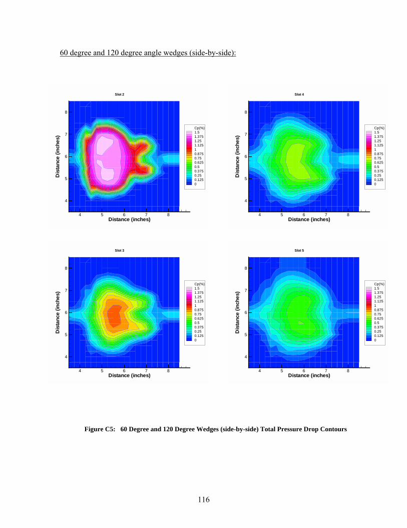
116




4

5

6

7

8

Dis

tanc

e(in

ches

)

Cp(%)1.51.3751.251.12510.8750.750.6250.50.3750.250.1250

Slot 2


4

5

6

7

8

Dis

tanc

e(in

ches

)

Cp(%)1.51.3751.251.12510.8750.750.6250.50.3750.250.1250

Slot 3


4

5

6

7

8

Dis

tanc

e(in

ches

)

Cp(%)1.51.3751.251.12510.8750.750.6250.50.3750.250.1250

Slot 4


4

5

6

7

8

Dis

tanc

e(in

ches

)

Cp(%)1.51.3751.251.12510.8750.750.6250.50.3750.250.1250

Slot 5

117




4

5

6

7

8

Dis

tanc

e(in

ches

)

Cp(%)1.51.3751.251.12510.8750.750.6250.50.3750.250.1250

Slot 2


4

5

6

7

8

Dis

tanc

e(in

ches

)

Cp(%)1.51.3751.251.12510.8750.750.6250.50.3750.250.1250

Slot 3


4

5

6

7

8

Dis

tanc

e(in

ches

)

Cp(%)1.51.3751.251.12510.8750.750.6250.50.3750.250.1250

Slot 4


4

5

6

7

8

Dis

tanc

e(in

ches

)

Cp(%)1.51.3751.251.12510.8750.750.6250.50.3750.250.1250

Slot 5

118

Appendix D - Comparison Plots for Horizontally Aligned Data

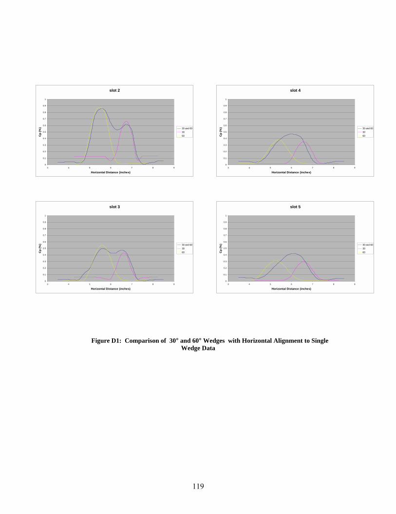
119

Figure D1: Comparison of 30° and 60° Wedges with Horizontal Alignment to Single Wedge Data

slot 2

0

0.1

0.2

0.3

0.4

0.5

0.6

0.7

0.8

0.9

1

3 4 5 6 7 8 9


Cp

(%) 30 and 60

3060

slot 3

0

0.1

0.2

0.3

0.4

0.5

0.6

0.7

0.8

0.9

1

3 4 5 6 7 8 9


Cp

(%) 30 and 60

3060

slot 4

0

0.1

0.2

0.3

0.4

0.5

0.6

0.7

0.8

0.9

1

3 4 5 6 7 8 9


Cp

(%) 30 and 60

3060

slot 5

0

0.1

0.2

0.3

0.4

0.5

0.6

0.7

0.8

0.9

1

3 4 5 6 7 8 9


Cp

(%) 30 and 60

3060

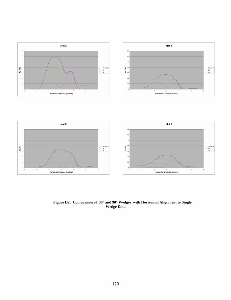
120


slot 2

0

0.2

0.4

0.6

0.8

1

1.2

1.4

3 4 5 6 7 8 9


Cp

(%) 30 and 90

3090

slot 3

0

0.2

0.4

0.6

0.8

1

1.2

1.4

3 4 5 6 7 8 9


Cp

(%) 30 and 90

3090

slot 4

0

0.2

0.4

0.6

0.8

1

1.2

1.4

3 4 5 6 7 8 9


Cp

(%) 30 and 90

3090

slot 5

0

0.2

0.4

0.6

0.8

1

1.2

1.4

3 4 5 6 7 8 9


Cp

(%) 30 and 90

3090

121


slot 2

0

0.2

0.4

0.6

0.8

1

1.2

1.4

1.6

3 4 5 6 7 8 9


Cp

(%) 30 and 120

30120

slot 3

0

0.2

0.4

0.6

0.8

1

1.2

1.4

1.6

3 4 5 6 7 8 9


Cp

(%) 30 and 120

30120

slot 4

0

0.2

0.4

0.6

0.8

1

1.2

1.4

1.6

3 4 5 6 7 8 9


Cp

(%) 30 and 120

30120

slot 5

0

0.2

0.4

0.6

0.8

1

1.2

1.4

1.6

3 4 5 6 7 8 9


Cp

(%) 30 and 120

30120

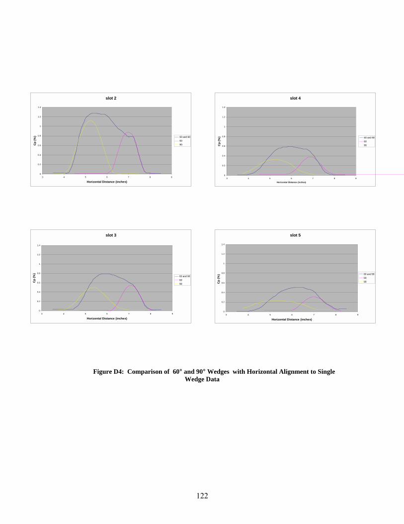
122


slot 2

0

0.2

0.4

0.6

0.8

1

1.2

1.4

3 4 5 6 7 8 9


Cp

(%) 60 and 90

6090

slot 3

0

0.2

0.4

0.6

0.8

1

1.2

1.4

3 4 5 6 7 8 9


Cp

(%)

60 and 906090

slot 4

0

0.2

0.4

0.6

0.8

1

1.2

1.4

3 4 5 6 7 8 9


Cp

(%) 60 and 90

6090

slot 5

0

0.2

0.4

0.6

0.8

1

1.2

1.4

3 4 5 6 7 8 9


Cp

(%) 60 and 90

6090

123


slot 2

0

0.2

0.4

0.6

0.8

1

1.2

1.4

1.6

3 4 5 6 7 8 9


Cp

(%) 60 and 120

6090

slot 3

0

0.2

0.4

0.6

0.8

1

1.2

1.4

1.6

3 4 5 6 7 8 9


Cp

(%) 60 and 120

60120

slot 4

0

0.2

0.4

0.6

0.8

1

1.2

1.4

1.6

3 4 5 6 7 8 9


Cp

(%)

60 and 12060120

slot 5

0

0.2

0.4

0.6

0.8

1

1.2

1.4

1.6

3 4 5 6 7 8 9


Cp

(%) 60 and 120

60120

124


slot 2

0

0.2

0.4

0.6

0.8

1

1.2

1.4

1.6

3 4 5 6 7 8 9


Cp

(%) 90 and 120

90120

slot 3

0

0.2

0.4

0.6

0.8

1

1.2

1.4

1.6

3 4 5 6 7 8 9


Cp

(%) 90 and 120

90120

slot 4

0

0.2

0.4

0.6

0.8

1

1.2

1.4

1.6

3 4 5 6 7 8 9


Cp

(%) 90 and 120

90120

slot 5

0

0.2

0.4

0.6

0.8

1

1.2

1.4

1.6

3 4 5 6 7 8 9


Cp

(%) 90 and 120

90120

125

Appendix E - Percent Total Pressure Drop Contour Plots for Combinations of Two Wedges Aligned Vertically

126

30 degree and 60 degree angle wedges (up and down):

Figure E1: 30 Degree and 60 Degree Wedges (up and down) Total Pressure Drop Contours


3

4

5

6

7

8

9

Dis

tanc

e(in

ches

)

Cp(%)1.51.3751.251.12510.8750.750.6250.50.3750.250.1250

Slot 2


3

4

5

6

7

8

9

Dis

tanc

e(in

ches

)

Cp(%)1.51.3751.251.12510.8750.750.6250.50.3750.250.1250

Slot 3


3

4

5

6

7

8

9

Dis

tanc

e(in

ches

)

Cp(%)1.51.3751.251.12510.8750.750.6250.50.3750.250.1250

Slot 4


3

4

5

6

7

8

9

Dis

tanc

e(in

ches

)

Cp(%)1.51.3751.251.12510.8750.750.6250.50.3750.250.1250

Slot 5

127




3

4

5

6

7

8

9

Dis

tanc

e(in

ches

)

Cp(%)1.51.3751.251.12510.8750.750.6250.50.3750.250.1250

Slot 2


3

4

5

6

7

8

9

Dis

tanc

e(in

ches

)

Cp(%)1.51.3751.251.12510.8750.750.6250.50.3750.250.1250

Slot 3


3

4

5

6

7

8

9

Dis

tanc

e(in

ches

)

Cp(%)1.51.3751.251.12510.8750.750.6250.50.3750.250.1250

Slot 4


3

4

5

6

7

8

9

Dis

tanc

e(in

ches

)

Cp(%)1.51.3751.251.12510.8750.750.6250.50.3750.250.1250

Slot 5

128


Figure E3: 30 Degree and 120 Degree wedges (up and down) Total Pressure Drop Contours


3

4

5

6

7

8

9

Dis

tanc

e(in

ches

)

Cp(%)1.51.3751.251.12510.8750.750.6250.50.3750.250.1250

Slot 2


3

4

5

6

7

8

9

Dis

tanc

e(in

ches

)

Cp(%)1.51.3751.251.12510.8750.750.6250.50.3750.250.1250

Slot 3


3

4

5

6

7

8

9

Dis

tanc

e(in

ches

)

Cp(%)1.51.3751.251.12510.8750.750.6250.50.3750.250.1250

Slot 4


3

4

5

6

7

8

9

Dis

tanc

e(in

ches

)

Cp(%)1.51.3751.251.12510.8750.750.6250.50.3750.250.1250

Slot 5

129




3

4

5

6

7

8

9

Dis

tanc

e(in

ches

)

Cp(%)1.51.3751.251.12510.8750.750.6250.50.3750.250.1250

Slot 2


3

4

5

6

7

8

9

Dis

tanc

e(in

ches

)

Cp(%)1.51.3751.251.12510.8750.750.6250.50.3750.250.1250

Slot 3


3

4

5

6

7

8

9

Dis

tanc

e(in

ches

)

Cp(%)1.51.3751.251.12510.8750.750.6250.50.3750.250.1250

Slot 4


3

4

5

6

7

8

9

Dis

tanc

e(in

ches

)

Cp(%)1.51.3751.251.12510.8750.750.6250.50.3750.250.1250

Slot 5

130




3

4

5

6

7

8

9

Dis

tanc

e(in

ches

)

Cp(%)1.51.3751.251.12510.8750.750.6250.50.3750.250.1250

Slot 2


3

4

5

6

7

8

9

Dis

tanc

e(in

ches

)

Cp(%)1.51.3751.251.12510.8750.750.6250.50.3750.250.1250

Slot 3


3

4

5

6

7

8

9

Dis

tanc

e(in

ches

)

Cp(%)1.51.3751.251.12510.8750.750.6250.50.3750.250.1250

Slot 4


3

4

5

6

7

8

9

Dis

tanc

e(in

ches

)

Cp(%)1.51.3751.251.12510.8750.750.6250.50.3750.250.1250

Slot 5

131




3

4

5

6

7

8

9

Dis

tanc

e(in

ches

)

Cp(%)1.51.3751.251.12510.8750.750.6250.50.3750.250.1250

Slot 2


3

4

5

6

7

8

9

Dis

tanc

e(in

ches

)

Cp(%)1.51.3751.251.12510.8750.750.6250.50.3750.250.1250

Slot 3


3

4

5

6

7

8

9

Dis

tanc

e(in

ches

)

Cp(%)1.51.3751.251.12510.8750.750.6250.50.3750.250.1250

Slot 4


3

4

5

6

7

8

9

Dis

tanc

e(in

ches

)

Cp(%)1.51.3751.251.12510.8750.750.6250.50.3750.250.1250

Slot 5

132

Appendix F - Comparison Plots for Vertically Aligned Data

133

Figure F1: Comparison of 30° and 60° Wedges with Vertical Alignment to Single Wedge Data

Slot 2

2

3

4

5

6

7

8

9

0 0.1 0.2 0.3 0.4 0.5 0.6 0.7 0.8 0.9

Cp (%)

Verti

cal D

ista

nce

(inch

es)

30 and 603060

Slot 5

2

3

4

5

6

7

8

9

10

0 0.1 0.2 0.3 0.4 0.5 0.6 0.7 0.8 0.9

Cp (%)

Ver

tical

Dis

tanc

e (in

ches

)

30 and 603060

Slot 4

2

3

4

5

6

7

8

9

10

0 0.1 0.2 0.3 0.4 0.5 0.6 0.7 0.8 0.9

Cp (%)

Verti

cal D

ista

nce

(inch

es)

30 and 6030 60

Slot 3

2

3

4

5

6

7

8

9

0 0.1 0.2 0.3 0.4 0.5 0.6 0.7 0.8 0.9

Cp (%)

Ver

tical

Dis

tanc

e (in

ches

)

30 and 603060

134

Figure F2: Comparison of 30° and 90° Wedges with Vertical Alignment to Single Wedge

Data

slot 2

2

3

4

5

6

7

8

9

0 0.2 0.4 0.6 0.8 1 1.2 1.4

Cp (%)

Ver

tical

Dis

tanc

e (in

ches

)

30 and 903090

slot 5

2

3

4

5

6

7

8

9

0 0.2 0.4 0.6 0.8 1 1.2

Cp (%)

Ver

tical

Dis

tanc

e (in

ches

)

30 and 903090

slot 3

2

3

4

5

6

7

8

9

0 0.2 0.4 0.6 0.8 1 1.2

Cp (%)

Ver

tical

Dis

tanc

e (in

ches

)

30 and 903090

slot 4

2

3

4

5

6

7

8

9

0 0.2 0.4 0.6 0.8 1 1.2

Cp (%)

Ver

tical

Dis

tanc

e (in

ches

)

30 and 903090

135


slot 2

2

3

4

5

6

7

8

9

0 0.2 0.4 0.6 0.8 1 1.2 1.4 1.6

Cp (%)

Ver

tical

Dis

tanc

e (in

ches

)

30 and 12030120

slot 5

2

3

4

5

6

7

8

9

0 0.2 0.4 0.6 0.8 1 1.2 1.4 1.6

Cp (%)

Ver

tical

Dis

tanc

e (in

ches

)

30 and 12030120

slot 3

2

3

4

5

6

7

8

9

0 0.2 0.4 0.6 0.8 1 1.2 1.4 1.6

Cp (%)

Ver

tical

Dis

tanc

e (in

ches

)

30 and 12030120

slot 4

2

3

4

5

6

7

8

9

0 0.2 0.4 0.6 0.8 1 1.2 1.4 1.6

Cp (%)

Ver

tical

Dis

tanc

e (in

ches

)

30 and 12030120

136


slot 2

2

3

4

5

6

7

8

9

0 0.2 0.4 0.6 0.8 1 1.2

Cp (%)

Ver

tical

Dis

tanc

e (in

ches

)

60 and 906090

slot 3

2

3

4

5

6

7

8

9

0 0.2 0.4 0.6 0.8 1 1.2

Cp (%)

Ver

tical

Dis

tanc

e (in

ches

)

60 and 906090

slot 4

2

3

4

5

6

7

8

9

0 0.2 0.4 0.6 0.8 1 1.2

Cp (%)

Ver

tical

Dis

tanc

e (in

ches

)

60 and 906090

slot 5

2

3

4

5

6

7

8

9

0 0.2 0.4 0.6 0.8 1 1.2

Cp (%)

Ver

tical

Dis

tanc

e (in

ches

)

60 and 906090

137


slot 2

2

3

4

5

6

7

8

9

0 0.2 0.4 0.6 0.8 1 1.2 1.4

Cp (%)

Ver

tical

Dis

tanc

e (in

ches

)

60 and 12060120

slot 3

2

3

4

5

6

7

8

9

0 0.2 0.4 0.6 0.8 1 1.2 1.4

Cp (%)

Ver

tical

Dis

tanc

e (in

ches

)

60 and 12060120

slot 4

2

3

4

5

6

7

8

9

0 0.2 0.4 0.6 0.8 1 1.2 1.4

Cp (%)

Ver

tical

Dis

tanc

e (in

ches

)

60 and 12060120

slot 5

2

3

4

5

6

7

8

9

0 0.2 0.4 0.6 0.8 1 1.2 1.4

Cp (%)

Ver

tical

Dis

tanc

e (in

ches

)

60 and 12060120

138


slot 2

2

3

4

5

6

7

8

9

10

0 0.2 0.4 0.6 0.8 1 1.2 1.4

Cp (%)

Ver

tical

Dis

tanc

e (in

ches

)

90 and 12090120

slot 3

2

3

4

5

6

7

8

9

10

0 0.2 0.4 0.6 0.8 1 1.2 1.4

Cp (%)

Ver

tical

Dis

tanc

e (in

ches

)

90 and 12090120

slot 4

2

3

4

5

6

7

8

9

10

0 0.2 0.4 0.6 0.8 1 1.2 1.4

Cp (%)

Vert

ical

Dis

tanc

e (in

ches

)

90 and 12090120

slot 5

2

3

4

5

6

7

8

9

10

0 0.2 0.4 0.6 0.8 1 1.2 1.4

Cp (%)

Ver

tical

Dis

tanc

e (in

ches

)

90 and 12090120

139

Appendix G – Uncertainty Analysis

140

Uncertainty Analysis:

An uncertainty analysis has been done on the experiment that was conducted in order to assess how much error existed. It was found that the opening angle of the splitting airfoil was accurate to +/- 1° due to the resolution that could be read from the protractor. The spatial resolution of the traverse was accurate to +/- 0.0625" due to the resolution of the scale.

The calibration curve, Figure 3.6, was used to find the error in the pressure measurements. This plot has a R value of 0.999 which shows that the curve is linear. This plot included the inclined manometer which was accurate to +/- 0.005 inches of water and also the voltage from the electronic manometer which was read on a multi-meter which was accurate to +/- 0.01 Volts. The equation of the calibration curve was:

bVmPressure +×=

where m = Slope of the line V = Voltage read by Labview b = Y-intercept The error was found for the slope which was defined as the errorm term in the following equation:

01.001.001.0005.0

12

12

±−±±−±

=±VVPPmm error

This value for the slope error was found to be equal to +/-0.0525. The error for the y-intercept was found which is represented by the errorb term in the following equation:

01.001.001.001.0005.0005.0 2

12

122 ±×

±−±±−±

−±=± VVVPPPbb error

The error for the y-intercept was found to be equal to +/- 0.0411. The voltage read by the data acquisition system was found to have an error of +/- 0.0049, since it was digitized with a 12-bit converter with a range of 10 to -10 volts. All of these errors were propagated through the calibration equation in order to find the errors for the pressure measurements, shown as errorPt in the following equation:

0411.00049.00525.0 ±+±×±=± bVmPtPt error

141

This error was found to be +/- 0.0465 inches of water for all of the total pressures measured. The electronic barometer used to measure the atmospheric pressure was accurate to +/- 0.041 inches of water. The error found in the pressure loss coefficient values, Cp, could be found by using the following formula:

100041.00465.0(max)0465.0)(0465.0(max) ×

±+±±−±=±

PatmPtyPtPtCpCp error

Cp error was found to be +/- 0.017%. An analysis was also done to see how repeatable the test results would be using this test setup. The upstream total pressure measured for each case was examined to see if the tunnel freestream conditions were consistent. Assuming a normal distribution about the mean value, the standard deviation was calculated from following formula:

21

N

1i

2i

1N

)x(xσ

−

−=∑

=

where

ix = Measured total pressure x = Mean of total pressure N= Number of samples

A sample of 80 free stream total pressure values for nominally identical flow conditions was used. It was found that the standard deviation was +/- 0.033 inches of water

142

Vita The author, son of Grant and Nancy Eddy, was born in 1976 in Richmond,

Virginia. He was raised in Richmond by his Stepfather, Lindsay Bruce, and his mother

after his father was deceased. He attended Douglas Freeman High School before

attending the Virginia Military Institute in Lexington, VA. There he was a member of

Tau Beta Pi an Phi Kappa Phi and was an academically distinguished graduate in 1999

from VMI with a B.S. in mechanical engineering. He began graduate studies in the Fall

of 1999 in the area of mechanical engineering at Virginia Tech. Upon graduation, he

plans to be employed with Bechtel Bettis in Charleston, S.C. pending a security

clearance.

study of steady-state wake characteristics of variable ... study of steady state wake...

Documents