study of mooring systems for offshore wave energy converters · com ondas regulares e irregulares....
TRANSCRIPT
FACULDADE DE ENGENHARIA DA UNIVERSIDADE DO PORTO
Study of Mooring Systems for OffshoreWave Energy Converters
Guilherme Moura Paredes
Programa Doutoral em Engenharia Civil
Supervisor: Francisco de Almeida Taveira Pinto
Second Supervisor: Luís Manuel de Carvalho Gato
November 14, 2016

c© Guilherme Moura Paredes, 2016

Study of Mooring Systems for Offshore Wave EnergyConverters
Guilherme Moura Paredes
Programa Doutoral em Engenharia Civil
November 14, 2016


Resumo
Os conversores flutuantes de energia das ondas necessitam de ser fixados de modo a impedir quefiquem à deriva no mar ou que sofram danos. No alto mar, com águas de profundidade intermédiaa elevada, a utilização de sistemas de amarração é uma opção atractiva por causa do seu custoreduzido. Devido às especificidades dos conversores flutuantes de energia das ondas (por exemploa necessidade de oscilar em ressonâcia), a concepção de soluções de amarração adequadas requero estudo de configurações de amarração diferentes das utilizadas em estruturas offshore mais co-muns. De modo a fornecer alguma assistência nesta tarefa, são apresentados três resultados: ummodelo numérico de cabos; uma técnica para seguir os movimentos de cabos de amarração emmodelos reduzidos; e dados experimentais sobre testes em modelo reduzido de diferentes config-urações de amarração. O modelo numérico de cabos utiliza o método de Galerkin com elementosespectrais/hp descontinuos, para resolver a equação diferencial parcial de cabos perfeitamenteflexíveis. Apresenta convergência exponencial para a solução e mostra algumas característicasque indicam ter a capacidade de capturar ondas de choque. A técnica de seguimento de cabosregista vídeos subaquáticos de cabos de amarração em modelos reduzidos, que são processadosutilizando um algorítmo especialmente desenvolvido para detectar e determinar a geometria doscabos em função do tempo. Toda a extensão do cabo é detectada, e não apenas alguns pontosseleccionados ao longo do seu comprimento, não havendo necessidade de utilizar interpolaçãopara reconstruir a geometria. As configurações de amarração estudadas em modelo reduzido sãoa catenária e duas configurações compactas, formadas por cabos tensos com flutuadores e pesosconcentrados. O modelo físico é composto por uma bóia cilíndrica, que representa um conversorflutuante de energia das ondas genérico, que é fixado por cada uma das configurações estudadas.São apresentados dados acerca das tensões máximas e mínimas nos cabos, dos deslocamentos dabóia, funções de transferência de primeira e segunda ordem, entre outros parâmetros, para ensaioscom ondas regulares e irregulares. As ferramentas e resultados indicados permitem tanto a in-vestigadores como a projectistas obter um conhecimento mais profundo sobre o comportamentodinâmico de cabos de amarração, e ter mais informação na altura de decidir a solução mais apro-priada para um sistema de amarração. O modelo numérico torna possível fazer a simulação deconversores amarrados em condições altamente dinâmicas, utilizado discretizações grosseiras. Atécnica para seguir o movimento de cabos pode ser utilizada tanto para a validação e calibraçãode simulações numéricas, como para determinar as regiões mais activas de cabos de amarração,desenvolver formulações e estudos mais avançados sobre o seu amortecimento, etc. Os resultadosexperimentais salientam as vantagens e desvantagens das três configurações estudadas, tornandomais fácil a selecção do melhor conceito conforme o dispositivo e a situação em causa.
i

ii

Abstract
Wave energy converters need to be secured to prevent them form drifting away in the sea or get-ting damaged. In offshore regions, with intermediate to deep waters, the use of mooring systemsto keep the converters on station is an attractive solution because of its reduced cost. Due to thespecificities of offshore wave energy converters (for example, the need to oscillate in resonance),the development of an appropriate mooring solution requires the study of mooring configurationsdifferent from those used in typical offshore structures. To provide some assistance in this task,three different outcomes are presented: a numerical model for mooring cables; a technique to trackmooring cables in small scale models; and results of experimental tests of small scale models ofdifferent mooring configurations. The numerical model uses the spectral/hp-element discontin-uous Galerkin method to solve the partial differential equation of perfectly flexible cables. Ithas exponential convergence to the solution and exhibits shock capturing features. The trackingtechnique records underwater videos of mooring cables in small scale models. These videos areprocessed using an especially developed algorithm that determines and outputs the geometry ofthe cable, represented by its medial axis, as a function of time. The cable is detected in its fulllength, and not only at selected points, so there is no need for interpolation to estimate its trueshape. The mooring configurations studied in small scale physical models are the chain catenary,and two compact configuration using taut cables, floaters and clumpweights. The physical modelis composed of a cylindrical buoy representing a generic wave energy converter that is kept onstation by the different mooring configurations studied. Data is provided about the maximum andminimum tension in the cables, the displacements of the buoy, the response amplitude operatorsfor the three configurations, among other parameters, when the model is subjected to regular andirregular waves. The tools and results mentioned allow researchers and developers to get a deeperinsight into the dynamic behaviour of mooring cables, and to have more information in the se-lection of an appropriate mooring configuration. The numerical model makes it possible to carryout simulations of moored devices in highly dynamic conditions using coarse discretisations. Thetechnique to track mooring cables can be used to validate numerical simulations, as well as to geta better understanding of the most active regions of mooring cables, accurate estimates of damp-ing, etc. The results from the experiments pin-point the advantages and disadvantages of the threeconfigurations studied, and make it easier to select the best one for a specific device and situation.
iii

iv

Acknowlegements
Although I am presented as the author of this thesis, it would not be possible to complete it withoutthe assistance of several people, whose contribution I wish to acknowledge.
I would like to thank my supervisor, Prof. Francisco de Almeida Taveira Pinto, from FEUP,and my co-supervisor, Prof. Luís Manuel de Carvalho Gato, from IST, for proposing the researchtopic and for their support throughout my work.
I also want to express my most sincere gratitude to my family not only for its support andpatience during my endeavour, but also for their additional insight and assistance in several tasks,and in particular my brother Miguel, for his companionship and encouragement.
A word of appreciation goes also to my Swedish friends, Johannes Palm, Claes Eskilssonand Lars “Lasse” Bergdahl. They have welcomed me during my mobility period in Sweden, atChalmers University of Technology and, more than assisting me in my research, they made mefeel at home. Their support and knowledge during and after my stay in Sweden were fundamentalfor the successful completion of my PhD work.
For his assistance in the tasks concerning image processing, I would also like to thank Prof.Miguel Fernando Paiva Velhote Correia, from FEUP.
I would also like to thank all my friends, who have been by my side during this time, keepingmy spirit and motivation up. In particular, my friends at FEUP, for the laughs and good momentswe shared, which contributed to an excellent work environment.
Finally, I acknowledge the support of Fundação para a Ciência e Tecnologia, for partiallyfunding my research through PhD grant SFRH/BD/62040/2009 and research project PTDC/EME-MFE/103524/2008, financed by the POPH/FSE program.
Guilherme Moura Paredes
v

vi

“By three methods we may learn wisdom: First, by reflection, which is noblest; Second, byimitation, which is easiest; and third by experience, which is the bitterest.”
Attributed to Chinese philosopher Confucius
vii

viii
Contents
List of Figures xiii
List of Tables xix
List of Symbols xxiii
1 Introduction 1
2 Literature Review 52.1 Modelling cable dynamics . . . . . . . . . . . . . . . . . . . . . . . . . . . . . 52.2 Mooring of wave energy converters . . . . . . . . . . . . . . . . . . . . . . . . 152.3 Tracking the motion of mooring cables . . . . . . . . . . . . . . . . . . . . . . . 22
3 Numerical Modelling of Mooring Cables 253.1 Introduction . . . . . . . . . . . . . . . . . . . . . . . . . . . . . . . . . . . . . 253.2 Spectral/hp-element Discontinuous Galerkin Method . . . . . . . . . . . . . . . 263.3 Cable Dynamics . . . . . . . . . . . . . . . . . . . . . . . . . . . . . . . . . . . 303.4 Numerical Model . . . . . . . . . . . . . . . . . . . . . . . . . . . . . . . . . . 323.5 Verification and Validation . . . . . . . . . . . . . . . . . . . . . . . . . . . . . 35
3.5.1 Verification . . . . . . . . . . . . . . . . . . . . . . . . . . . . . . . . . 353.5.2 Validation . . . . . . . . . . . . . . . . . . . . . . . . . . . . . . . . . . 37
3.6 Moored Buoy Simulation . . . . . . . . . . . . . . . . . . . . . . . . . . . . . . 403.7 Discussion . . . . . . . . . . . . . . . . . . . . . . . . . . . . . . . . . . . . . . 493.8 Conclusions . . . . . . . . . . . . . . . . . . . . . . . . . . . . . . . . . . . . . 50
4 Tracking Mooring Cables in Physical Models 514.1 Introduction . . . . . . . . . . . . . . . . . . . . . . . . . . . . . . . . . . . . . 514.2 Optical Concepts . . . . . . . . . . . . . . . . . . . . . . . . . . . . . . . . . . 524.3 Experimental Set-up . . . . . . . . . . . . . . . . . . . . . . . . . . . . . . . . 564.4 Tracking Technique - Experimental Procedure . . . . . . . . . . . . . . . . . . . 62
4.4.1 Calibration . . . . . . . . . . . . . . . . . . . . . . . . . . . . . . . . . 644.4.2 Video Acquisition . . . . . . . . . . . . . . . . . . . . . . . . . . . . . 66
4.5 Tracking Technique - Processing Algorithm . . . . . . . . . . . . . . . . . . . . 674.6 Case Studies . . . . . . . . . . . . . . . . . . . . . . . . . . . . . . . . . . . . . 724.7 Error Analysis . . . . . . . . . . . . . . . . . . . . . . . . . . . . . . . . . . . . 744.8 Discussion . . . . . . . . . . . . . . . . . . . . . . . . . . . . . . . . . . . . . . 764.9 Conclusions . . . . . . . . . . . . . . . . . . . . . . . . . . . . . . . . . . . . . 78
ix

x CONTENTS
5 Physical Modelling of Mooring Configurations 795.1 Introduction . . . . . . . . . . . . . . . . . . . . . . . . . . . . . . . . . . . . . 795.2 Mooring Design . . . . . . . . . . . . . . . . . . . . . . . . . . . . . . . . . . . 81
5.2.1 Design Procedure . . . . . . . . . . . . . . . . . . . . . . . . . . . . . . 815.2.2 Design Data . . . . . . . . . . . . . . . . . . . . . . . . . . . . . . . . . 83
5.3 Experimental Set-up . . . . . . . . . . . . . . . . . . . . . . . . . . . . . . . . 845.4 Experimental Methods . . . . . . . . . . . . . . . . . . . . . . . . . . . . . . . 965.5 Data Processing . . . . . . . . . . . . . . . . . . . . . . . . . . . . . . . . . . . 985.6 Results and Discussion . . . . . . . . . . . . . . . . . . . . . . . . . . . . . . . 102
5.6.1 Quasi-static Displacement Tests . . . . . . . . . . . . . . . . . . . . . . 1025.6.2 Decay Tests . . . . . . . . . . . . . . . . . . . . . . . . . . . . . . . . . 1035.6.3 Regular Waves . . . . . . . . . . . . . . . . . . . . . . . . . . . . . . . 1065.6.4 Irregular Waves . . . . . . . . . . . . . . . . . . . . . . . . . . . . . . . 113
5.7 Additional Remarks . . . . . . . . . . . . . . . . . . . . . . . . . . . . . . . . . 1215.8 Conclusions . . . . . . . . . . . . . . . . . . . . . . . . . . . . . . . . . . . . . 122
6 Conclusions 125
7 Suggested Future Developments 1297.1 Numerical Model for Mooring Cables . . . . . . . . . . . . . . . . . . . . . . . 1297.2 Tracking Technique for Mooring Cables in Physical Models . . . . . . . . . . . 1307.3 Experimental Work . . . . . . . . . . . . . . . . . . . . . . . . . . . . . . . . . 130
A Mooring Design 133A.1 Design Loads and Displacements . . . . . . . . . . . . . . . . . . . . . . . . . . 133A.2 Equations of Static Equilibrium of the Mooring Configurations . . . . . . . . . . 134
B Sea-state Definition 137
C Usage of Equipment 139C.1 Wave Tank . . . . . . . . . . . . . . . . . . . . . . . . . . . . . . . . . . . . . . 139C.2 Load Cells and Wave Probes . . . . . . . . . . . . . . . . . . . . . . . . . . . . 139
C.2.1 Load Cells . . . . . . . . . . . . . . . . . . . . . . . . . . . . . . . . . 140C.2.2 Wave Probes . . . . . . . . . . . . . . . . . . . . . . . . . . . . . . . . 140
C.3 Motion Capture . . . . . . . . . . . . . . . . . . . . . . . . . . . . . . . . . . . 142C.4 Centre of Gravity . . . . . . . . . . . . . . . . . . . . . . . . . . . . . . . . . . 142C.5 Moment of Inertia . . . . . . . . . . . . . . . . . . . . . . . . . . . . . . . . . . 146C.6 Calibration of the Floaters . . . . . . . . . . . . . . . . . . . . . . . . . . . . . 146
D Uncertainty Analysis 149D.1 General Method . . . . . . . . . . . . . . . . . . . . . . . . . . . . . . . . . . . 149D.2 Calibrated Masses . . . . . . . . . . . . . . . . . . . . . . . . . . . . . . . . . . 150D.3 Height of the Buoy . . . . . . . . . . . . . . . . . . . . . . . . . . . . . . . . . 151D.4 Diameter of the Buoy . . . . . . . . . . . . . . . . . . . . . . . . . . . . . . . . 152D.5 Determination of the Centre of Gravity . . . . . . . . . . . . . . . . . . . . . . . 152D.6 Determination of the Moment of Inertia . . . . . . . . . . . . . . . . . . . . . . 157D.7 Clumpweights . . . . . . . . . . . . . . . . . . . . . . . . . . . . . . . . . . . . 162D.8 Floaters . . . . . . . . . . . . . . . . . . . . . . . . . . . . . . . . . . . . . . . 162
D.8.1 Diameter . . . . . . . . . . . . . . . . . . . . . . . . . . . . . . . . . . 162

CONTENTS xi
D.8.2 Mass and Buoyancy . . . . . . . . . . . . . . . . . . . . . . . . . . . . 163D.9 Chain and Cable Properties . . . . . . . . . . . . . . . . . . . . . . . . . . . . . 164
D.9.1 Mass and Submerged Weight per Unit Length . . . . . . . . . . . . . . . 164D.9.2 Dimensions of the Chain . . . . . . . . . . . . . . . . . . . . . . . . . . 167D.9.3 Stiffness . . . . . . . . . . . . . . . . . . . . . . . . . . . . . . . . . . . 167
D.10 Oscillation Periods . . . . . . . . . . . . . . . . . . . . . . . . . . . . . . . . . 169D.11 Load Cells . . . . . . . . . . . . . . . . . . . . . . . . . . . . . . . . . . . . . . 180D.12 Load Cell Attachments . . . . . . . . . . . . . . . . . . . . . . . . . . . . . . . 180D.13 Draft . . . . . . . . . . . . . . . . . . . . . . . . . . . . . . . . . . . . . . . . . 181D.14 Calibration Errors . . . . . . . . . . . . . . . . . . . . . . . . . . . . . . . . . . 184
D.14.1 Calibration of the Wave Probes . . . . . . . . . . . . . . . . . . . . . . . 185D.14.2 Calibration of the Load Cells . . . . . . . . . . . . . . . . . . . . . . . . 189
Bibliography 191

xii CONTENTS

List of Figures
3.1 Illustration of the variables in the spectral/hp-element discontinuous Galerkin method.The indexes l and r indicate, respectively, the left and right borders of the elements. 29
3.2 Representation of the variables used to describe the dynamics of a cable. . . . . . 303.3 L2 norm of the error, ‖E ‖L2 , in the simulation of the elastic catenary. . . . . . . . 363.4 L2 norm of the error, ‖E ‖L2 , in the simulation of the vibrating string. . . . . . . . 373.5 Experimental set-up simulated to validate the numerical model. . . . . . . . . . . 373.6 Measured and simulated tension for the rotation period T = 3,50s. . . . . . . . . 393.7 Measured and simulated tension for the rotation period T = 1,25s. . . . . . . . . 393.8 Experimental set-up reproduced in the simulation of the moored buoy. . . . . . . 413.9 Hull of the buoy, made of a stainless steel frame wrapped in a polyethylene sheet. 413.10 Placement of the load cell. . . . . . . . . . . . . . . . . . . . . . . . . . . . . . 423.11 Comparison of experimental data and simulated results for regular waves with
height H = 0,088m and period T = 1,30s. . . . . . . . . . . . . . . . . . . . . . 463.12 Comparison of experimental data and simulated results for regular waves with
height H = 0,100m and period T = 1,40s. . . . . . . . . . . . . . . . . . . . . . 473.13 Comparison of experimental data and simulated results for regular waves with
height H = 0,122m and period T = 1,50s. . . . . . . . . . . . . . . . . . . . . . 48
4.1 Representation of pincushion and barrel distortion on a square pattern. . . . . . . 524.2 Keystone effect. When a face of an object is projected onto an oblique plane, the
shapes in the resulting projection are not geometrically similar to the ones in theobject. . . . . . . . . . . . . . . . . . . . . . . . . . . . . . . . . . . . . . . . . 54
4.3 Dilation. The origin of the structuring element (marked with ×) is matched toeach of the pixels in the initial shape (marked with ) and its pixels added together,resulting in the dilated shape. . . . . . . . . . . . . . . . . . . . . . . . . . . . . 55
4.4 Thinning. Successively reducing the thickness of a shape will result in a one-pixelwide stroke that is approximately the medial axis of the shape. . . . . . . . . . . 55
4.5 The top-hat transform. . . . . . . . . . . . . . . . . . . . . . . . . . . . . . . . 564.6 Panoramic view of the experimental set-up. The buoy (A) is in the centre with the
mooring cables (B) extending to the left and to the right of it. On the right bottomcorner is the housing (C) with the video camera (standing on a tripod). Floodlights(D) can be seen on the right part of the image. Beneath the buoy is a black filmapplied on the floor (E) and behind the buoy is a vertical black curtain (F). Thewave generator (G) and the absorption beach (H) are in the top right and top leftcorners of the image. . . . . . . . . . . . . . . . . . . . . . . . . . . . . . . . . 57
4.7 Side view of the experimental set-up. . . . . . . . . . . . . . . . . . . . . . . . . 574.8 Top view of the experimental set-up. . . . . . . . . . . . . . . . . . . . . . . . . 584.9 Components of the imaging system used to record the motions of the cables. . . . 59
xiii

xiv LIST OF FIGURES
4.10 Photograph of a mooring cable taken through a flat port. The water depth is0,900 m and the span of the cable is 5,59 m. The small field of view caused bythe flat port of the housing made it impossible to capture the entire length of thecable. Pincushion distortion is also visible in the image, causing the edges of thepit to appear curved. . . . . . . . . . . . . . . . . . . . . . . . . . . . . . . . . 60
4.11 Underwater photograph of the cable with minimal contrast enhancement, showinga foggy haze caused by the suspended dirt in the water of the wave tank. . . . . . 60
4.12 Saturation of the image caused by vertical light reflecting off the floor (on the left).The saturated region blocks the visibility of the portion of the chain near the cornerof the pit. . . . . . . . . . . . . . . . . . . . . . . . . . . . . . . . . . . . . . . 61
4.13 Target used for the experimental steps of linearisation and calibration. . . . . . . 624.14 Examples of some photographs of the target during linearisation, in different ori-
entations and positions along the plane of the cable. . . . . . . . . . . . . . . . . 634.15 Position of the target during the calibration phase. . . . . . . . . . . . . . . . . . 644.16 Local reference frame of the calibration target as established by the “Camera Cal-
ibration Toolbox for MATLAB”. The zt axis is not shown because it is almostperpendicular to the photograph. . . . . . . . . . . . . . . . . . . . . . . . . . . 65
4.17 Points used for the calibration of the experimental set-up. . . . . . . . . . . . . . 654.18 First frame of the processed clip, after correcting the distortion and the keystone
effect. The cable is not in static equilibrium, because the clip was extracted from alonger video. The image histogram has been modified to enhance visibility whenprinted. . . . . . . . . . . . . . . . . . . . . . . . . . . . . . . . . . . . . . . . 67
4.19 Initial search region (enclosed by the white contour) provided to the algorithmto assist in the detection the cable. The image histogram has been modified toenhance visibility when printed. . . . . . . . . . . . . . . . . . . . . . . . . . . 68
4.20 The result of applying the top hat transform to the search region. Contrast hasbeen enhanced over the entire image so that the result of the top-hat transform isclear, because this transform lowers the intensity of the processed regions. . . . . 69
4.21 The result of applying the Canny edged detector: the outline of the cable is effi-ciently traced. . . . . . . . . . . . . . . . . . . . . . . . . . . . . . . . . . . . . 69
4.22 Example of an extraneous streak that will interfere in the detection of the cable.These streaks are caused by the application of the Canny edged detector. Thisimage is taken from a later portion of the clip to illustrate this problem. . . . . . . 69
4.23 Outline of the cable filled in using dilation. . . . . . . . . . . . . . . . . . . . . 704.24 Medial axis of the cable completely extracted from the image. . . . . . . . . . . 704.25 Cable profile calibrated to the model reference frame defined in section 4.4.1. . . 714.26 New search region, automatically defined by the processing algorithm based on
the medial axis of the cable. . . . . . . . . . . . . . . . . . . . . . . . . . . . . 714.27 Flowchart of the algorithm used to process the videos. . . . . . . . . . . . . . . . 724.28 Experimental set-up after removing the curtain. The background has now sev-
eral shades with varying intensity, random objects and distinct edges that mightinterfere with the algorithm. The image histogram has been modified to enhancevisibility when printed. . . . . . . . . . . . . . . . . . . . . . . . . . . . . . . . 73
4.29 Detected profile of the cable in the experimental set-up without the vertical curtain,in waves with height H = 0,04m and period T = 2,33s. Even though there areseveral perturbations in the background, the cable is fully detected. . . . . . . . . 73

LIST OF FIGURES xv
4.30 Interference of the non-uniform background. The area of the background betweenthe plastic film on the floor and the black block is a bright strip that is merged withthe cable when the top-hat transform is applied. The image histogram has beenmodified to enhance visibility when printed. . . . . . . . . . . . . . . . . . . . . 73
4.31 Gap in the detected profile of the cable caused by the interference of the background. 744.32 Comparison of the measured profile of the cable with the profile obtained from the
equation of the inelastic catenary. . . . . . . . . . . . . . . . . . . . . . . . . . . 75
5.1 Schematics of the tested configurations: CON1 on the top, CON2 in the centreand CAT on bottom. . . . . . . . . . . . . . . . . . . . . . . . . . . . . . . . . . 80
5.2 Photographs of the hull (on the left) and of the rubber ballast (on the right). . . . 855.3 Cross section of the hull of the buoy showing the bulge. The deformation caused
by the bulge on the bottom is not significant when compared with the regularthickness of the hull. . . . . . . . . . . . . . . . . . . . . . . . . . . . . . . . . 85
5.4 Dimensions of the mooring configurations. . . . . . . . . . . . . . . . . . . . . . 875.5 Top view of the experimental set-up. . . . . . . . . . . . . . . . . . . . . . . . . 885.6 Fully assembled components of a mooring leg of CON2. All the mooring compo-
nents used in the compact configurations are shown: the mooring cable with theacrylic floater and calibration weights (on the top left), the fishing weights usedfor the clumpweights (on the top right), and the anchor plate (on the bottom). . . 88
5.7 Sample of the synthetic cable used for the compact configurations. . . . . . . . . 895.8 Sample of the chain used in the CAT mooring. . . . . . . . . . . . . . . . . . . . 905.9 Top view of the anchor with its removable anchor plate (the silver grey plate in the
centre). . . . . . . . . . . . . . . . . . . . . . . . . . . . . . . . . . . . . . . . 905.10 Adapters used for attaching the cables and load cells to the buoy. On the left side
of the adapter a pulley is installed that was meant to guide the cable to the load cell,which would be fixed to the right side of the adapter. However, this arrangementwas abandoned. . . . . . . . . . . . . . . . . . . . . . . . . . . . . . . . . . . . 91
5.11 Load cell (the small steel square) used to measure the tension force in the mooringcables, with the holding rings (used to connect the load cell to the cable and to theadapter) screwed in. . . . . . . . . . . . . . . . . . . . . . . . . . . . . . . . . . 91
5.12 Installation of the adapter on the buoy. (a) general view of the adapter; (b) detailedview of the adapter, showing its orientation and position. . . . . . . . . . . . . . 92
5.13 Inline assembly of the load cell. A - load cell adapter; B - shackle securing theload cell to the adapter; C - load cell; D - mooring cable. . . . . . . . . . . . . . 92
5.14 Infrared system used to track the motions of the buoy: (a) markers; (b) infra-redcameras standing on tripods on the upper catwalk. . . . . . . . . . . . . . . . . . 93
5.15 Panorama view of the experimental set-up for CON1. The model is in the centre.On the left of the photograph is the absorption beach and on the right is the wavegenerator. On the bottom of the photograph are the bars that hold the wave probes. 94
5.16 Photographs of the tested configurations assembled in the wave tank. . . . . . . . 955.17 Effects of filtering. . . . . . . . . . . . . . . . . . . . . . . . . . . . . . . . . . 985.18 Restoring force as a function of the surge displacement: (a) CON1; (b) CON2; (c)
CAT. . . . . . . . . . . . . . . . . . . . . . . . . . . . . . . . . . . . . . . . . . 995.19 Determination of the damping. (a) Example of least squares fitting a straight line
to the extremes of the natural logarithm of the decaying motion of one test; (b)decay curve determined using the mean exponential argument of all the tests andthe initial position ξ0 of the displayed sample record. . . . . . . . . . . . . . . . 100

xvi LIST OF FIGURES
5.20 Comparison between the measured and the linear displacement component (inthis case, surge). The linear component is estimated by extracting the first ordercomponent of the measured motion spectrum. . . . . . . . . . . . . . . . . . . . 102
5.21 Secant stiffness of the configurations. The oscillations near zero displacement aredue to the division of the force value by very small displacements. . . . . . . . . 102
5.22 Response amplitude operator for surge. (a) response for a regular wave height H =0,04m; (b) response for a regular wave height H = 0,08m. ξ1 - surge displacementamplitude; "Rep." denotes the repeated tests. . . . . . . . . . . . . . . . . . . . . 107
5.23 Response amplitude operator for heave. (a) response for a regular wave heightH = 0,04m; (b) response for a regular wave height H = 0,08m. ξ3 - heave dis-placement amplitude; "Rep." denotes the repeated tests. . . . . . . . . . . . . . . 107
5.24 Response amplitude operator for pitch. (a) response for a regular wave height H =0,04m; (b) response for a regular wave height H = 0,08m. ξ5 - pitch displacementamplitude "Rep." denotes the repeated tests. . . . . . . . . . . . . . . . . . . . . 108
5.25 Decaying amplitude of the heave motion in regular waves with period T = 1,05s. 1095.26 Non-dimensionl mean surge drift. . . . . . . . . . . . . . . . . . . . . . . . . . 1095.27 Non-dimensional maximum tension. . . . . . . . . . . . . . . . . . . . . . . . . 1115.28 Non-dimensional dynamic tension. . . . . . . . . . . . . . . . . . . . . . . . . . 1115.29 Non-dimensional mean tension. . . . . . . . . . . . . . . . . . . . . . . . . . . 1125.30 Shape of the tension cycles of the three configurations in regular waves with H =
0,08m and T = 1,13s, showing multiple peaks per cycle. . . . . . . . . . . . . . 1135.31 Rank of maximum surge displacements of the three configurations in the survival
sea-states. . . . . . . . . . . . . . . . . . . . . . . . . . . . . . . . . . . . . . . 1175.32 Distribution of surge displacements with the corresponding zero-crossing periods
of the three configurations in the survival sea-states. . . . . . . . . . . . . . . . . 1175.33 Time series of the tension in cable 1 in the survival sea-states. (a) - (c) SURV1;
(d) - (f) SURV2. . . . . . . . . . . . . . . . . . . . . . . . . . . . . . . . . . . . 1205.34 Rank of peak tensions and associated dynamic tensions for the three configurations
in survival sea-states. (a) SURV1; (b) SURV2 . . . . . . . . . . . . . . . . . . . 121
A.1 Free body diagram for CON1. FF - buoyancy force of the floaters. . . . . . . . . 134A.2 Free body diagram for CON2. FF - buoyancy force of the floaters; FS - submerged
weight of the clumpweights. . . . . . . . . . . . . . . . . . . . . . . . . . . . . 135A.3 Horizontal components of the restoring force. Frx - horizontal restoring force in
the x direction; τih - horizontal component of the tension force in cable i. . . . . . 136
C.1 Set-up for calibration of the load cells. The load cell is the small square rectangleon the top of the image, from which a load is hanging on a hook. . . . . . . . . . 141
C.2 Schematics of the procedure for the determination of the centre of gravity. Cg -centre of gravity; Cr - centre of rotation. . . . . . . . . . . . . . . . . . . . . . . 142
C.3 Steel wedge screwed to the hull of the buoy used in the determination of the centreof gravity. . . . . . . . . . . . . . . . . . . . . . . . . . . . . . . . . . . . . . . 143
C.4 Buoy with the wedges resting on steel supports. . . . . . . . . . . . . . . . . . . 144C.5 Determination of the centre of gravity. An external load (the hexagonal steel mass)
is hanging from to the top of the hull by a string and the rotation angle α is mea-sured by the inclinometer on the styrofoam lid. The buoy is resting on the steelframes by its side. . . . . . . . . . . . . . . . . . . . . . . . . . . . . . . . . . . 144
C.6 Nomenclature of the directions of the horizontal axes on the buoy. . . . . . . . . 145

LIST OF FIGURES xvii
C.7 Schematics of the set-up used to determine the inertia of buoy. dRC - distance fromthe pivot point R to the centre of gravity Cg. . . . . . . . . . . . . . . . . . . . . 146
D.1 Estimation of the distance dRC. The cable that goes around the pivot point andaround the attachment to the hull has a thickness e. . . . . . . . . . . . . . . . . 158
D.2 Variables in the determination of the draft. . . . . . . . . . . . . . . . . . . . . . 181

xviii LIST OF FIGURES

List of Tables
3.1 Parameters of the experimental set-up. . . . . . . . . . . . . . . . . . . . . . . . 383.2 Properties of the model buoy. mb - mass; Db - diameter; Hb - height; ycg - position
of the centre of gravity above the bottom of the buoy; db - draft; Icf - inertia aroundthe horizontal axis through the centre of flotation. . . . . . . . . . . . . . . . . . 41
3.3 Properties of the chain. . . . . . . . . . . . . . . . . . . . . . . . . . . . . . . . 423.4 Hydrodynamic coefficients of the buoy. . . . . . . . . . . . . . . . . . . . . . . 443.5 Characteristics of the ground used in the simulation of the moored buoy. . . . . . 45
4.1 Intrinsic parameters of the imaging system. . . . . . . . . . . . . . . . . . . . . 644.2 Coordinates of the calibration points in the model reference frame. . . . . . . . . 66
5.1 Considered irregular sea-states in prototype scale. . . . . . . . . . . . . . . . . 845.2 Irregular sea-states in model scale. OP - operational; SURV - survival. . . . . . . 845.3 Properties of the buoy. . . . . . . . . . . . . . . . . . . . . . . . . . . . . . . . 865.4 Draft of the buoy for each configuration. . . . . . . . . . . . . . . . . . . . . . . 865.5 Pre-tension in the cables. . . . . . . . . . . . . . . . . . . . . . . . . . . . . . . 865.6 Mass of the mooring configurations. CAT* accounts only for the portions of the
chains suspended when in rest position. . . . . . . . . . . . . . . . . . . . . . . 865.7 Properties of the floaters. Indexes 1, 2 and 3 refer to the cable where the floater
was installed. . . . . . . . . . . . . . . . . . . . . . . . . . . . . . . . . . . . . 875.8 Properties of the clumpweights. Indexes 1, 2 and 3 refer to the cable where the
clumpweight was installed. . . . . . . . . . . . . . . . . . . . . . . . . . . . . . 895.9 Properties of the synthetic cables. . . . . . . . . . . . . . . . . . . . . . . . . . 895.10 Properties of the chain. . . . . . . . . . . . . . . . . . . . . . . . . . . . . . . . 905.11 Damped natural periods of the buoy. . . . . . . . . . . . . . . . . . . . . . . . . 1035.12 Hydrodynamic parameters for surge. . . . . . . . . . . . . . . . . . . . . . . . . 1045.13 Hydrodynamic parameters for heave. . . . . . . . . . . . . . . . . . . . . . . . . 1045.14 Hydrodynamic parameters for pitch. . . . . . . . . . . . . . . . . . . . . . . . . 1055.15 Desired and measured sea-state parameters for the irregular wave tests. . . . . . . 1135.16 Displacement in operational sea-states. ξ1 - surge; ξ3 - heave; ξ5 - pitch; p.p -
peak-to-peak amplitude. Overbar denotes mean value. . . . . . . . . . . . . . . . 1145.17 Tension in operational sea-states. τ - tension; p.p - peak-to-peak amplitude. Over-
bar denotes mean value. Indexes 1 and 2 refer to the cable where the tension wasmeasured. . . . . . . . . . . . . . . . . . . . . . . . . . . . . . . . . . . . . . . 115
5.18 Displacements in survival sea-states. ξ1 - surge; ξ3 - heave; ξ5 - pitch; p.p - peak-to-peak amplitude. Overbar denotes mean value. . . . . . . . . . . . . . . . . . . 116
5.19 Tension in survival sea-states.p.p - peak-to-peak amplitude. Overbar denotes mean value.Indexes 1 and 2 refer to the cable where the tension was measured. . . . . . . . . 119
xix

xx LIST OF TABLES
A.1 First order horizonal displacements of the free buoy estimated using linear poten-tial theory. . . . . . . . . . . . . . . . . . . . . . . . . . . . . . . . . . . . . . . 133
A.2 Parameters for the estimation of the second order wave forces. . . . . . . . . . . 134
B.1 Distribution of wave heights and periods for the Northwest quadrant offshoreFigueira da Foz. . . . . . . . . . . . . . . . . . . . . . . . . . . . . . . . . . . . 137
B.2 Distribution of wave heights and periods for the West quadrant offshore Figueirada Foz. . . . . . . . . . . . . . . . . . . . . . . . . . . . . . . . . . . . . . . . . 137
B.3 Wave height and period distribution for the combined West and Northwest quad-rants offshore Figueira da Foz. . . . . . . . . . . . . . . . . . . . . . . . . . . . 138
B.4 Estimated yearly available energy distribution offshore Figueira da Foz (W·year/m).138B.5 Selected irregular sea-states. . . . . . . . . . . . . . . . . . . . . . . . . . . . . 138
C.1 Readings of the signal of the load cells before and after submergence. LC - Loadcell. . . . . . . . . . . . . . . . . . . . . . . . . . . . . . . . . . . . . . . . . . 140
C.2 Loads applied in the calibration of the load cells. . . . . . . . . . . . . . . . . . 141
D.1 Properties of the masses used in the determination of the centre of gravity and inthe calibration of the load cells. . . . . . . . . . . . . . . . . . . . . . . . . . . . 150
D.2 Measurements of the height of the buoy. . . . . . . . . . . . . . . . . . . . . . . 151D.3 Estimation of the uncertainty in the height of the buoy. . . . . . . . . . . . . . . 151D.4 Measurements of the diameter of the buoy. . . . . . . . . . . . . . . . . . . . . . 152D.5 Estimation of the uncertainty in the diameter of the buoy. . . . . . . . . . . . . . 152D.6 Value of the parameters required for the estimation of the uncertainty in the posi-
tion of the centre of gravity. . . . . . . . . . . . . . . . . . . . . . . . . . . . . . 153D.7 Measurements of the distance dcc. . . . . . . . . . . . . . . . . . . . . . . . . . 154D.8 Partial derivatives of equation D.6 with respect to its variables, for each measure-
ment presented in Table D.7. . . . . . . . . . . . . . . . . . . . . . . . . . . . . 155D.9 Systematic uncertainty due to the different variables of equation D.6 for each mea-
surement presented in Table D.7. . . . . . . . . . . . . . . . . . . . . . . . . . . 156D.10 Estimation of the uncertainty in the position of the centre of gravity of the buoy. . 157D.11 Measurements of dc and d1. . . . . . . . . . . . . . . . . . . . . . . . . . . . . . 158D.12 Estimated values of dRC. . . . . . . . . . . . . . . . . . . . . . . . . . . . . . . 158D.13 Average value and uncertainty of dRC for the two directions used in the determi-
nation of the moment of inertia of buoy. . . . . . . . . . . . . . . . . . . . . . . 159D.14 Average oscillation period of the buoy and systematic uncertainty in the tests for
the determination of the moment of inertia. . . . . . . . . . . . . . . . . . . . . 159D.15 Partial derivatives of equation D.13 with respect to its variables, for each measure-
ment presented in Table D.14. . . . . . . . . . . . . . . . . . . . . . . . . . . . 160D.16 Systematic uncertainty due to the different variables of equation D.13 for each
measurement presented in Table D.14. . . . . . . . . . . . . . . . . . . . . . . . 160D.17 Estimation of the uncertainty in moment of inertia through the centre of gravity of
the buoy. . . . . . . . . . . . . . . . . . . . . . . . . . . . . . . . . . . . . . . . 161D.18 Uncertainty in the mass and submerged weight of the clumpweights. . . . . . . . 162D.19 Measurements of the perimeter of the floaters. . . . . . . . . . . . . . . . . . . . 162D.20 Partial derivatives of equation D.16 with respect to its variables, for each measure-
ment presented in Table D.19. . . . . . . . . . . . . . . . . . . . . . . . . . . . 163D.21 Uncertainty in the diameter of the floaters. . . . . . . . . . . . . . . . . . . . . . 163D.22 Mass of the floaters and respective uncertainty. . . . . . . . . . . . . . . . . . . 163

LIST OF TABLES xxi
D.23 Buoyancy of the floaters and respective uncertainty. . . . . . . . . . . . . . . . . 163D.24 Measurement of the mass and length of 10 samples of chain. . . . . . . . . . . . 164D.25 Partial derivatives of equation D.18 with respect to its variables, for each measure-
ment presented in Table D.24. . . . . . . . . . . . . . . . . . . . . . . . . . . . 165D.26 Systematic uncertainty due to the different variables of equation D.18 for each
measurement presented in Table D.24. . . . . . . . . . . . . . . . . . . . . . . . 165D.27 Estimation of the uncertainty in the mass per unit length of the chain. . . . . . . . 165D.28 Measurement of the submerged weight and length of 5 samples of chain. . . . . . 165D.29 Partial derivatives of equation D.18 with respect to its variables, for each measure-
ment presented in Table D.28. . . . . . . . . . . . . . . . . . . . . . . . . . . . 166D.30 Systematic uncertainty due to the different variables of equation D.18 for each
measurement presented in Table D.28. . . . . . . . . . . . . . . . . . . . . . . . 166D.31 Estimation of the uncertainty in the submerged weight per unit length of the chain. 166D.32 Estimation of the uncertainty in the mass and submerged weight per unit length of
the synthetic cable. . . . . . . . . . . . . . . . . . . . . . . . . . . . . . . . . . 166D.33 Measurements of the dimensions of 10 samples of chain links. . . . . . . . . . . 167D.34 Estimation of the uncertainty in the dimensions of the chain links. X represents
each of the three dimensions analysed. . . . . . . . . . . . . . . . . . . . . . . . 167D.35 Length of the samples as reported officially, lr, and as taken from the test notes, ln. 168D.36 Axial stiffness of the samples of synthetic cable and chain. . . . . . . . . . . . . 168D.37 Uncertainty estimates in the stiffness of the synthetic cable and of the chain. . . . 168D.38 Measured heave resonance periods for the free buoy. . . . . . . . . . . . . . . . 170D.39 Estimated heave resonance period and uncertainty for the free buoy. . . . . . . . 170D.40 Measured pitch resonance periods for the free buoy. . . . . . . . . . . . . . . . . 171D.41 Estimated pitch resonance period and uncertainty for the free buoy. . . . . . . . . 171D.42 Measured surge resonance periods for CON1. . . . . . . . . . . . . . . . . . . . 171D.43 Estimated surge resonance period and uncertainty for CON1. . . . . . . . . . . . 172D.44 Measured heave resonance periods for CON1. . . . . . . . . . . . . . . . . . . . 172D.45 Estimated heave resonance period and uncertainty for CON1. . . . . . . . . . . . 172D.46 Measured pitch resonance periods for CON1. . . . . . . . . . . . . . . . . . . . 173D.47 Estimated pitch resonance period and uncertainty for CON1. . . . . . . . . . . . 173D.48 Measured surge resonance periods for CON2. . . . . . . . . . . . . . . . . . . . 174D.49 Estimated surge resonance period and uncertainty for CON2. . . . . . . . . . . . 174D.50 Measured heave resonance periods for CON2. . . . . . . . . . . . . . . . . . . . 175D.51 Estimated heave resonance period and uncertainty for CON2. . . . . . . . . . . . 175D.52 Measured pitch resonance periods for CON2. . . . . . . . . . . . . . . . . . . . 176D.53 Estimated pitch resonance period and uncertainty for CON2. . . . . . . . . . . . 176D.54 Measured surge resonance periods for the catenary. . . . . . . . . . . . . . . . . 177D.55 Estimated surge resonance period and uncertainty for the catenary. . . . . . . . . 177D.56 Measured heave resonance periods for the catenary. . . . . . . . . . . . . . . . . 178D.57 Estimated heave resonance period and uncertainty for the catenary. . . . . . . . . 178D.58 Measured pitch resonance periods for the catenary. . . . . . . . . . . . . . . . . 179D.59 Estimated pitch resonance period and uncertainty for the catenary. . . . . . . . . 179D.60 Mass of the load cells. . . . . . . . . . . . . . . . . . . . . . . . . . . . . . . . 180D.61 Mass of the load cell adapters. . . . . . . . . . . . . . . . . . . . . . . . . . . . 180D.62 Average value and uncertainty of the mass of the load cell adapters. . . . . . . . 180D.63 Freeboard and draft of the free buoy. . . . . . . . . . . . . . . . . . . . . . . . . 181D.64 Uncertainty in the draft for the free buoy. . . . . . . . . . . . . . . . . . . . . . 181

xxii LIST OF TABLES
D.65 Freeboard and draft of the buoy in CON1. . . . . . . . . . . . . . . . . . . . . . 182D.66 Uncertainty in the draft of the buoy in CON1. . . . . . . . . . . . . . . . . . . . 182D.67 Freeboard and draft of the buoy in CON2. . . . . . . . . . . . . . . . . . . . . . 182D.68 Uncertainty in the draft of the buoy in CON2. . . . . . . . . . . . . . . . . . . . 182D.69 Freeboard and draft of the buoy moored with the catenary. . . . . . . . . . . . . 182D.70 Uncertainty in the draft of the buoy moored with the catenary. . . . . . . . . . . 183D.71 Parameters of the least squares fit for each calibration of the wave probes. . . . . 186D.72 Parameters for the estimation of the uncertainty in the wave probe calibration due
to the least squares fit. . . . . . . . . . . . . . . . . . . . . . . . . . . . . . . . . 187D.73 Estimate of the uncertainty in the calibration of the wave probes. . . . . . . . . . 188D.74 Parameters of the least squares fit for the calibration of the load cells. . . . . . . . 189D.75 Parameters for the estimation of the uncertainty in the calibration of the load cells
due to the least squares fit. . . . . . . . . . . . . . . . . . . . . . . . . . . . . . 189D.76 Estimate of the uncertainty in the calibration of the load cells. . . . . . . . . . . . 189

List of Symbols
‖E ‖L2 L2 norm of the error of the numerical solution . . . . . . . . . . . . . . . . . . . . . . . . . . . . . . . . . . . . . 35
A Amplitude of a linear wave on a cable . . . . . . . . . . . . . . . . . . . . . . . . . . . . . . . . . . . . . . . . . . . . . . . . 36
a Wave amplitude . . . . . . . . . . . . . . . . . . . . . . . . . . . . . . . . . . . . . . . . . . . . . . . . . . . . . . . . . . . . . . . . . . . 106
A0 Nominal cross-section of the cable for calculations involving elasticity . . . . . . . . . . . . . . . . . . 31
A1 Nominal cross-section of the cable for hydrodynamic added mass force calculations . . . . . . 31
A Added mass matrix of a floating body . . . . . . . . . . . . . . . . . . . . . . . . . . . . . . . . . . . . . . . . . . . . . . . . 43
ae Non-dimensional acceleration vector of the cable in element e . . . . . . . . . . . . . . . . . . . . . . . . . . 33
Ai j Entry i, j of the added mass matrix A . . . . . . . . . . . . . . . . . . . . . . . . . . . . . . . . . . . . . . . . . . . . . . . . 44
arel Relative acceleration between the cable and the water . . . . . . . . . . . . . . . . . . . . . . . . . . . . . . . . 31
aw Water acceleration . . . . . . . . . . . . . . . . . . . . . . . . . . . . . . . . . . . . . . . . . . . . . . . . . . . . . . . . . . . . . . . . . 31
B Radiation damping matrix of a floating body . . . . . . . . . . . . . . . . . . . . . . . . . . . . . . . . . . . . . . . . . . 43
brb Radiation damping coefficient of the buoy . . . . . . . . . . . . . . . . . . . . . . . . . . . . . . . . . . . . . . . . . . . 103
btb Total damping coefficient of the buoy, including non-linear effects . . . . . . . . . . . . . . . . . . . . . 101
bD Dirichlet boundary condition . . . . . . . . . . . . . . . . . . . . . . . . . . . . . . . . . . . . . . . . . . . . . . . . . . . . . . . 34
Bi j Entry i, j of the damping matrix matrix B . . . . . . . . . . . . . . . . . . . . . . . . . . . . . . . . . . . . . . . . . . . . 44
btm Total damping coefficient of the mooring system, including non-linear effects . . . . . . . . . . 101
bN Newmann boundary condition . . . . . . . . . . . . . . . . . . . . . . . . . . . . . . . . . . . . . . . . . . . . . . . . . . . . . . 34
bt Damping coefficient of the buoy-mooring system. . . . . . . . . . . . . . . . . . . . . . . . . . . . . . . . . . . . . 101
bX Systematic uncertainty in quantity X . . . . . . . . . . . . . . . . . . . . . . . . . . . . . . . . . . . . . . . . . . . . . . . 149
biX Systematic uncertainty in quantity X due to variable i . . . . . . . . . . . . . . . . . . . . . . . . . . . . . . . . 150
C Stiffness matrix of a floating body . . . . . . . . . . . . . . . . . . . . . . . . . . . . . . . . . . . . . . . . . . . . . . . . . . . 43
c Celerity of a linear wave on a cable . . . . . . . . . . . . . . . . . . . . . . . . . . . . . . . . . . . . . . . . . . . . . . . . . . . 36
C0 Set of continuous functions without continuous derivatives . . . . . . . . . . . . . . . . . . . . . . . . . . . . 25
xxiii

xxiv List of Symbols
Cdn Hydrodynamic normal drag coefficient of the cable . . . . . . . . . . . . . . . . . . . . . . . . . . . . . . . . . . 31
Cdt Hydrodynamic tangential drag coefficient of the cable . . . . . . . . . . . . . . . . . . . . . . . . . . . . . . . . 31
CFD Computational fluid dynamics . . . . . . . . . . . . . . . . . . . . . . . . . . . . . . . . . . . . . . . . . . . . . . . . . . . . 15
Cm Hydrodynamic added mass coefficient of the cable . . . . . . . . . . . . . . . . . . . . . . . . . . . . . . . . . . . 31
d Minimum size of a detail resolved by the imaging system . . . . . . . . . . . . . . . . . . . . . . . . . . . . . . . 66
D0 Nominal diameter of the cable for the calculation of the hydrodynamic drag forces . . . . . . . 31
D1 Nominal diameter of the cable for the calculation of seabed forces . . . . . . . . . . . . . . . . . . . . . 32
Db Buoy diameter . . . . . . . . . . . . . . . . . . . . . . . . . . . . . . . . . . . . . . . . . . . . . . . . . . . . . . . . . . . . . . . . . . . . 41
db Buoy draft . . . . . . . . . . . . . . . . . . . . . . . . . . . . . . . . . . . . . . . . . . . . . . . . . . . . . . . . . . . . . . . . . . . . . . . . 41
DFi Diameter of floater i . . . . . . . . . . . . . . . . . . . . . . . . . . . . . . . . . . . . . . . . . . . . . . . . . . . . . . . . . . . . . 162
dRC Distance between the centre of gravity and the pivot point R in the set-up for determinationof the inertia . . . . . . . . . . . . . . . . . . . . . . . . . . . . . . . . . . . . . . . . . . . . . . . . . . . . . . . . . . . . . . . . . . . 146
E Elasticity modulus . . . . . . . . . . . . . . . . . . . . . . . . . . . . . . . . . . . . . . . . . . . . . . . . . . . . . . . . . . . . . . . . . . 31
E Error in the numerical solution . . . . . . . . . . . . . . . . . . . . . . . . . . . . . . . . . . . . . . . . . . . . . . . . . . . . . . 35
f Buoy freeboard . . . . . . . . . . . . . . . . . . . . . . . . . . . . . . . . . . . . . . . . . . . . . . . . . . . . . . . . . . . . . . . . . . . . . 86
f General numerical flux across the boundaries of element e . . . . . . . . . . . . . . . . . . . . . . . . . . . . . . 28
fdn Vector of hydrodynamic normal drag acting on the cable . . . . . . . . . . . . . . . . . . . . . . . . . . . . . . 31
fdt Vector of hydrodynamic tangential drag acting on the cable . . . . . . . . . . . . . . . . . . . . . . . . . . . . 31
fext Vector of distributed external forces acting on a cable . . . . . . . . . . . . . . . . . . . . . . . . . . . . . . . . . 30
fext Non-dimensional vector of external forces acting on the cable . . . . . . . . . . . . . . . . . . . . . . . . . 32
fbuoy Vector sum of external forces acting on a floating body . . . . . . . . . . . . . . . . . . . . . . . . . . . . . . 43
FF Floater buoyancy force . . . . . . . . . . . . . . . . . . . . . . . . . . . . . . . . . . . . . . . . . . . . . . . . . . . . . . . . . . . . 134
fm Vector of hydrodynamic added mass force acting on the cable . . . . . . . . . . . . . . . . . . . . . . . . . . 31
Frx horizontal restoring force in the x direction . . . . . . . . . . . . . . . . . . . . . . . . . . . . . . . . . . . . . . . . . 136
FS Clumpweight submerged weight . . . . . . . . . . . . . . . . . . . . . . . . . . . . . . . . . . . . . . . . . . . . . . . . . . . 135
fsn Normal force applied by the seabed on the cable . . . . . . . . . . . . . . . . . . . . . . . . . . . . . . . . . . . . . . 32
fst Tangential force applied by the seabed on the cable . . . . . . . . . . . . . . . . . . . . . . . . . . . . . . . . . . . . 32
fw Vector of first order wave forces acting on a floating body . . . . . . . . . . . . . . . . . . . . . . . . . . . . . . 43
Fxp Mean horizontal wave drift force . . . . . . . . . . . . . . . . . . . . . . . . . . . . . . . . . . . . . . . . . . . . . . . . . . . 82
Fxs Horizontal component of the slowly varying wave loads . . . . . . . . . . . . . . . . . . . . . . . . . . . . . . . 82

List of Symbols xxv
g Magnitude of the acceleration of gravity . . . . . . . . . . . . . . . . . . . . . . . . . . . . . . . . . . . . . . . . . . . . . . 32
g Acceleration of gravity . . . . . . . . . . . . . . . . . . . . . . . . . . . . . . . . . . . . . . . . . . . . . . . . . . . . . . . . . . . . . . 31
H Regular wave height . . . . . . . . . . . . . . . . . . . . . . . . . . . . . . . . . . . . . . . . . . . . . . . . . . . . . . . . . . . . . . . . 42
h Characteristic size of a finite element discretisation. . . . . . . . . . . . . . . . . . . . . . . . . . . . . . . . . . . . . 25
h Non-dimensional characteristic size of the finite element discretisation . . . . . . . . . . . . . . . . . . . 34
Hb Buoy height . . . . . . . . . . . . . . . . . . . . . . . . . . . . . . . . . . . . . . . . . . . . . . . . . . . . . . . . . . . . . . . . . . . . . . 41
Hm0 Estimate of the significant wave height using the zero-order spectral moment . . . . . . . . . 138
H∗s Increased value of the largest significant wave height of the design sea-states . . . . . . . . . . . . 82
Hs−max Maximum significant wave height of the design sea-states . . . . . . . . . . . . . . . . . . . . . . . . 133
I Image intensity . . . . . . . . . . . . . . . . . . . . . . . . . . . . . . . . . . . . . . . . . . . . . . . . . . . . . . . . . . . . . . . . . . . . . 52
Icf Inertia of the buoy relative to a horizontal axis through the centre of floatation . . . . . . . . . . . 41
Icg Inertia of the buoy relative to a horizontal axis through the centre of gravity . . . . . . . . . . . . . 85
k Wave slope. . . . . . . . . . . . . . . . . . . . . . . . . . . . . . . . . . . . . . . . . . . . . . . . . . . . . . . . . . . . . . . . . . . . . . . . 106
Kb Hydrodynamic stiffness of the buoy . . . . . . . . . . . . . . . . . . . . . . . . . . . . . . . . . . . . . . . . . . . . . . . . 101
Km Stiffness of the mooring system . . . . . . . . . . . . . . . . . . . . . . . . . . . . . . . . . . . . . . . . . . . . . . . . . . . 101
Ks Seabed stiffness modulus per unit volume . . . . . . . . . . . . . . . . . . . . . . . . . . . . . . . . . . . . . . . . . . . . 32
Kt Stiffness of the buoy-mooring system . . . . . . . . . . . . . . . . . . . . . . . . . . . . . . . . . . . . . . . . . . . . . . . 100
L Stretched length of a cable . . . . . . . . . . . . . . . . . . . . . . . . . . . . . . . . . . . . . . . . . . . . . . . . . . . . . . . . . . . 36
l Cable sample length . . . . . . . . . . . . . . . . . . . . . . . . . . . . . . . . . . . . . . . . . . . . . . . . . . . . . . . . . . . . . . . . 164
lc Characteristic length . . . . . . . . . . . . . . . . . . . . . . . . . . . . . . . . . . . . . . . . . . . . . . . . . . . . . . . . . . . . . . . . 32
LDG Local discontinuous Galerkin . . . . . . . . . . . . . . . . . . . . . . . . . . . . . . . . . . . . . . . . . . . . . . . . . . . . 14
LOWESS Locally weighted scatterplot smoothing . . . . . . . . . . . . . . . . . . . . . . . . . . . . . . . . . . . . . . . 98
Lt Length covered by the camera in a specified direction on the image . . . . . . . . . . . . . . . . . . . . . 66
M Generalised mass matrix of a floating body . . . . . . . . . . . . . . . . . . . . . . . . . . . . . . . . . . . . . . . . . . . 43
ma Added mass of the buoy-mooring system . . . . . . . . . . . . . . . . . . . . . . . . . . . . . . . . . . . . . . . . . . . 100
mab Added mass of the buoy . . . . . . . . . . . . . . . . . . . . . . . . . . . . . . . . . . . . . . . . . . . . . . . . . . . . . . . . . . 103
Me Elemental mass matrix . . . . . . . . . . . . . . . . . . . . . . . . . . . . . . . . . . . . . . . . . . . . . . . . . . . . . . . . . . . . 28
Mei j Entry i, j of the elemental mass matrix Me . . . . . . . . . . . . . . . . . . . . . . . . . . . . . . . . . . . . . . . . . . 28
mb Mass of the buoy . . . . . . . . . . . . . . . . . . . . . . . . . . . . . . . . . . . . . . . . . . . . . . . . . . . . . . . . . . . . . . . . . . 41
mabe Experimentally determined added mass of the buoy . . . . . . . . . . . . . . . . . . . . . . . . . . . . . . . . . 104

xxvi List of Symbols
mtb Total mass of the buoy, including added mass . . . . . . . . . . . . . . . . . . . . . . . . . . . . . . . . . . . . . . . 101
mc Mass of a sample of cable . . . . . . . . . . . . . . . . . . . . . . . . . . . . . . . . . . . . . . . . . . . . . . . . . . . . . . . . . 164
ml mass of the cable per unit length . . . . . . . . . . . . . . . . . . . . . . . . . . . . . . . . . . . . . . . . . . . . . . . . . . . . 30
mlc Characteristic mass per unit length . . . . . . . . . . . . . . . . . . . . . . . . . . . . . . . . . . . . . . . . . . . . . . . . . . 32
mtm Total mass of the mooring system, including added mass . . . . . . . . . . . . . . . . . . . . . . . . . . . . 101
mt Total mass of the buoy-mooring system, including added mass . . . . . . . . . . . . . . . . . . . . . . . . 100
Nc Numerical filter cut-off term . . . . . . . . . . . . . . . . . . . . . . . . . . . . . . . . . . . . . . . . . . . . . . . . . . . . . . . . 45
Np Number of pixels along a certain length Lt in an image . . . . . . . . . . . . . . . . . . . . . . . . . . . . . . . . 66
ns Unit outward normal vector to the seabed . . . . . . . . . . . . . . . . . . . . . . . . . . . . . . . . . . . . . . . . . . . . 32
p Highest order of the polynomial basis functions used in hp-elements . . . . . . . . . . . . . . . . . . . . . 25
P Average wave power density per unit surface area and crest width . . . . . . . . . . . . . . . . . . . . . . 138
PFi Perimeter of floater i . . . . . . . . . . . . . . . . . . . . . . . . . . . . . . . . . . . . . . . . . . . . . . . . . . . . . . . . . . . . . . 162
pn Position of the fairlead of the mooring cables at time instant tn . . . . . . . . . . . . . . . . . . . . . . . . . 45
q Non-dimensional tangent vector to the cable . . . . . . . . . . . . . . . . . . . . . . . . . . . . . . . . . . . . . . . . . . . 33
qe Approximate numerical solution to the tangent vector q on element e . . . . . . . . . . . . . . . . . . . 33
qej Vector of polynomial coefficients of the local numerical solution qe in element e . . . . . . . . . 33
r Buoy radius . . . . . . . . . . . . . . . . . . . . . . . . . . . . . . . . . . . . . . . . . . . . . . . . . . . . . . . . . . . . . . . . . . . . . . . . 82
r Position of a material point of the cable in a Cartesian reference frame . . . . . . . . . . . . . . . . . . . 30
RAO Response amplitude operator . . . . . . . . . . . . . . . . . . . . . . . . . . . . . . . . . . . . . . . . . . . . . . . . . . . . 106
r Non-dimensional position vector . . . . . . . . . . . . . . . . . . . . . . . . . . . . . . . . . . . . . . . . . . . . . . . . . . . . . 32re Numerical flux of re on element e . . . . . . . . . . . . . . . . . . . . . . . . . . . . . . . . . . . . . . . . . . . . . . . . . . . 33
re Approximate numerical solution to the position vector r on element e . . . . . . . . . . . . . . . . . . . 33
rej Vector of polynomial coefficients of the local numerical solution re in element e . . . . . . . . . 33
RKDG Runge-Kutta discontinuous Galerkin . . . . . . . . . . . . . . . . . . . . . . . . . . . . . . . . . . . . . . . . . . . . 14
rx x component of the position vector r . . . . . . . . . . . . . . . . . . . . . . . . . . . . . . . . . . . . . . . . . . . . . . . . . 35
ry y component of the position vector r . . . . . . . . . . . . . . . . . . . . . . . . . . . . . . . . . . . . . . . . . . . . . . . . . 36
rz z component of the position vector r . . . . . . . . . . . . . . . . . . . . . . . . . . . . . . . . . . . . . . . . . . . . . . . . . 35
s Lagrangian coordinate measured along the unstretched length of the cable . . . . . . . . . . . . . . . . 30
s Non-dimensional lagrangian coordinate along the cable . . . . . . . . . . . . . . . . . . . . . . . . . . . . . . . . . 32
sX Random uncertainty in quantity X . . . . . . . . . . . . . . . . . . . . . . . . . . . . . . . . . . . . . . . . . . . . . . . . . . 149

List of Symbols xxvii
siX Random uncertainty in quantity X due to variable i . . . . . . . . . . . . . . . . . . . . . . . . . . . . . . . . . . . 150
T Oscillation period . . . . . . . . . . . . . . . . . . . . . . . . . . . . . . . . . . . . . . . . . . . . . . . . . . . . . . . . . . . . . . . . . . 37
t Time . . . . . . . . . . . . . . . . . . . . . . . . . . . . . . . . . . . . . . . . . . . . . . . . . . . . . . . . . . . . . . . . . . . . . . . . . . . . . . . 26
T02 Spectral moment relation to approximate Tz . . . . . . . . . . . . . . . . . . . . . . . . . . . . . . . . . . . . . . . . . . 83
t Tangent vector to the cable . . . . . . . . . . . . . . . . . . . . . . . . . . . . . . . . . . . . . . . . . . . . . . . . . . . . . . . . . . . 30
tc Characteristic time . . . . . . . . . . . . . . . . . . . . . . . . . . . . . . . . . . . . . . . . . . . . . . . . . . . . . . . . . . . . . . . . . 32
Te Energy period . . . . . . . . . . . . . . . . . . . . . . . . . . . . . . . . . . . . . . . . . . . . . . . . . . . . . . . . . . . . . . . . . . . . 138
tn Time instant n . . . . . . . . . . . . . . . . . . . . . . . . . . . . . . . . . . . . . . . . . . . . . . . . . . . . . . . . . . . . . . . . . . . . . 45
TP Peak period of an irregular sea-state . . . . . . . . . . . . . . . . . . . . . . . . . . . . . . . . . . . . . . . . . . . . . . . . . 83
ts Unit vector in the direction of the tangential velocity of the cable relative to the seabed . . . . 32
t Non-dimensional time . . . . . . . . . . . . . . . . . . . . . . . . . . . . . . . . . . . . . . . . . . . . . . . . . . . . . . . . . . . . . . . 32
Tz Mean zero down-crossing period of an irregular sea-state . . . . . . . . . . . . . . . . . . . . . . . . . . . . . . 83
u Line coordinate of a digital image . . . . . . . . . . . . . . . . . . . . . . . . . . . . . . . . . . . . . . . . . . . . . . . . . . . . 52
δ u Approximate numerical solution to the solution u of a partial differential equation . . . . . . . . 26
δ ue Local approximate numerical solution to the solution u of a partial differential equation . . 27
δ u j Polynomial coefficients for the approximate solution δ u . . . . . . . . . . . . . . . . . . . . . . . . . . . . . . 26
δ uej Polynomial coefficients of the local approximate numerical solution δ ue in element e . . . . 27
ue Vector with local polynomial coefficients uej . . . . . . . . . . . . . . . . . . . . . . . . . . . . . . . . . . . . . . . . . . 28
uel Value of the numerical solution at the left boundary of element e . . . . . . . . . . . . . . . . . . . . . . . 29
uer Value of the numerical solution at the right boundary of element e . . . . . . . . . . . . . . . . . . . . . . 29
UV Ultra-violet light . . . . . . . . . . . . . . . . . . . . . . . . . . . . . . . . . . . . . . . . . . . . . . . . . . . . . . . . . . . . . . . . . 61
uX Standard uncertainty in quantity X . . . . . . . . . . . . . . . . . . . . . . . . . . . . . . . . . . . . . . . . . . . . . . . . . 149
UXk% Expanded uncertainty in quantity X to a confidence interval of k percent . . . . . . . . . . . . . 149
v Column coordinate of a digital image . . . . . . . . . . . . . . . . . . . . . . . . . . . . . . . . . . . . . . . . . . . . . . . . . 52
ve Non-dimensional velocity vector of the cable in element e . . . . . . . . . . . . . . . . . . . . . . . . . . . . . 33
vlim Limiting velocity for the ramping of the seabed friction coefficient µs . . . . . . . . . . . . . . . . . . 32
vrel Relative velocity between the cable and the water . . . . . . . . . . . . . . . . . . . . . . . . . . . . . . . . . . . . 31
vsn Magnitude of the velocity of the cable in the normal direction to the seabed . . . . . . . . . . . . . 32
vst Velocity of the cable in the tangential direction to the seabed . . . . . . . . . . . . . . . . . . . . . . . . . . . 32
vw Water velocity . . . . . . . . . . . . . . . . . . . . . . . . . . . . . . . . . . . . . . . . . . . . . . . . . . . . . . . . . . . . . . . . . . . . 31

xxviii List of Symbols
w Vector of first order wave force coefficients . . . . . . . . . . . . . . . . . . . . . . . . . . . . . . . . . . . . . . . . . . . 43
wi Entry i of the wave force coefficient vector w . . . . . . . . . . . . . . . . . . . . . . . . . . . . . . . . . . . . . . . . . 44
x Cartesian coordinate x . . . . . . . . . . . . . . . . . . . . . . . . . . . . . . . . . . . . . . . . . . . . . . . . . . . . . . . . . . . . . . . 30
xel Value of the Cartesian coordinate x at the left boundary of element e . . . . . . . . . . . . . . . . . . . . 29
xm x axis of the model reference frame . . . . . . . . . . . . . . . . . . . . . . . . . . . . . . . . . . . . . . . . . . . . . . . . . . 65
xmax Maximum allowed horizontal displacement for a floating structure . . . . . . . . . . . . . . . . . . . . 81
xer Value of the Cartesian coordinate x at the right boundary of element e . . . . . . . . . . . . . . . . . . . 29
xs Displacement of a floating structure caused by second order wave loads . . . . . . . . . . . . . . . . . 81
xt x axis of the calibration target reference frame. . . . . . . . . . . . . . . . . . . . . . . . . . . . . . . . . . . . . . . . . 64
xw Displacement of a floating structure caused by first order wave loads . . . . . . . . . . . . . . . . . . . . 81
y Cartesian coordinate y . . . . . . . . . . . . . . . . . . . . . . . . . . . . . . . . . . . . . . . . . . . . . . . . . . . . . . . . . . . . . . . 30
ycg Position of the centre of gravity of the buoy relative to the bottom . . . . . . . . . . . . . . . . . . . . . . 41
ym y axis of the model reference frame . . . . . . . . . . . . . . . . . . . . . . . . . . . . . . . . . . . . . . . . . . . . . . . . . . 65
yt y axis of the calibration target reference frame. . . . . . . . . . . . . . . . . . . . . . . . . . . . . . . . . . . . . . . . . 64
z Cartesian coordinate z . . . . . . . . . . . . . . . . . . . . . . . . . . . . . . . . . . . . . . . . . . . . . . . . . . . . . . . . . . . . . . . 30
zm z axis of the model reference frame . . . . . . . . . . . . . . . . . . . . . . . . . . . . . . . . . . . . . . . . . . . . . . . . . . 65
zt z axis of the calibration target reference frame . . . . . . . . . . . . . . . . . . . . . . . . . . . . . . . . . . . . . . . . . 64
α Angle . . . . . . . . . . . . . . . . . . . . . . . . . . . . . . . . . . . . . . . . . . . . . . . . . . . . . . . . . . . . . . . . . . . . . . . . . . . . 134
β Angle . . . . . . . . . . . . . . . . . . . . . . . . . . . . . . . . . . . . . . . . . . . . . . . . . . . . . . . . . . . . . . . . . . . . . . . . . . . . 134
Γ Numerical filter parameter . . . . . . . . . . . . . . . . . . . . . . . . . . . . . . . . . . . . . . . . . . . . . . . . . . . . . . . . . . . 45
γc Submerged weight of a sample of cable . . . . . . . . . . . . . . . . . . . . . . . . . . . . . . . . . . . . . . . . . . . . . 164
γJ JONSWAP spectrum shape parameter . . . . . . . . . . . . . . . . . . . . . . . . . . . . . . . . . . . . . . . . . . . . . . . . 83
γl submerged weight of the cable per unit length . . . . . . . . . . . . . . . . . . . . . . . . . . . . . . . . . . . . . . . . . 31
δ Phase angle . . . . . . . . . . . . . . . . . . . . . . . . . . . . . . . . . . . . . . . . . . . . . . . . . . . . . . . . . . . . . . . . . . . . . . . 100
δδδ Vector of phase angles . . . . . . . . . . . . . . . . . . . . . . . . . . . . . . . . . . . . . . . . . . . . . . . . . . . . . . . . . . . . . . 43
∆H Depth of penetration of the cable in the seabed. . . . . . . . . . . . . . . . . . . . . . . . . . . . . . . . . . . . . . . 32
δi Entry i of the phase vector δδδ . . . . . . . . . . . . . . . . . . . . . . . . . . . . . . . . . . . . . . . . . . . . . . . . . . . . . . . . 44
∆t Integration time-step/acquisition interval . . . . . . . . . . . . . . . . . . . . . . . . . . . . . . . . . . . . . . . . . . . . . 43
ε Extension of the cable . . . . . . . . . . . . . . . . . . . . . . . . . . . . . . . . . . . . . . . . . . . . . . . . . . . . . . . . . . . . . . . 30

List of Symbols xxix
ζ Damping factor . . . . . . . . . . . . . . . . . . . . . . . . . . . . . . . . . . . . . . . . . . . . . . . . . . . . . . . . . . . . . . . . . . . 100
ζs Seabed damping factor . . . . . . . . . . . . . . . . . . . . . . . . . . . . . . . . . . . . . . . . . . . . . . . . . . . . . . . . . . . . . 32
η Water surface elevation . . . . . . . . . . . . . . . . . . . . . . . . . . . . . . . . . . . . . . . . . . . . . . . . . . . . . . . . . . . . . 43
θ Angle . . . . . . . . . . . . . . . . . . . . . . . . . . . . . . . . . . . . . . . . . . . . . . . . . . . . . . . . . . . . . . . . . . . . . . . . . . . . 135
κ Numerical flux direction control parameter . . . . . . . . . . . . . . . . . . . . . . . . . . . . . . . . . . . . . . . . . . . . 34
Λ Numerical filter parameter . . . . . . . . . . . . . . . . . . . . . . . . . . . . . . . . . . . . . . . . . . . . . . . . . . . . . . . . . . 45
λ1 Local discontinuous Galerkin numerical flux penalty . . . . . . . . . . . . . . . . . . . . . . . . . . . . . . . . . . 34
λ2 Additional flux penalty to the local discontinuous Galerkin numerical flux . . . . . . . . . . . . . . . 34
λl Geometrical scale of a physical model . . . . . . . . . . . . . . . . . . . . . . . . . . . . . . . . . . . . . . . . . . . . . . . 84
λt Time scale of the physical model . . . . . . . . . . . . . . . . . . . . . . . . . . . . . . . . . . . . . . . . . . . . . . . . . . . . 97
µs Seabed kinetic friction coefficient . . . . . . . . . . . . . . . . . . . . . . . . . . . . . . . . . . . . . . . . . . . . . . . . . . . 32
ξ Displacement of the buoy in a specified degree of freedom . . . . . . . . . . . . . . . . . . . . . . . . . . . . 100
ξ0 Initial displacement of the buoy in a specified degree of freedom . . . . . . . . . . . . . . . . . . . . . . 100
ξ1 Surge displacement amplitude . . . . . . . . . . . . . . . . . . . . . . . . . . . . . . . . . . . . . . . . . . . . . . . . . . . . . 106
ξ1 Mean surge displacement . . . . . . . . . . . . . . . . . . . . . . . . . . . . . . . . . . . . . . . . . . . . . . . . . . . . . . . . . . 109
ξ3 Heave displacement amplitude . . . . . . . . . . . . . . . . . . . . . . . . . . . . . . . . . . . . . . . . . . . . . . . . . . . . . 106
ξ5 Pitch displacement amplitude . . . . . . . . . . . . . . . . . . . . . . . . . . . . . . . . . . . . . . . . . . . . . . . . . . . . . . 106
ξξξ Displacement vector of a floating structure . . . . . . . . . . . . . . . . . . . . . . . . . . . . . . . . . . . . . . . . . . . . 43
ξξξ Velocity vector of a floating structure . . . . . . . . . . . . . . . . . . . . . . . . . . . . . . . . . . . . . . . . . . . . . . . . . 43
ξξξ Acceleration vector of a floating structure . . . . . . . . . . . . . . . . . . . . . . . . . . . . . . . . . . . . . . . . . . . . . 43
ρc Density of the material of the cable . . . . . . . . . . . . . . . . . . . . . . . . . . . . . . . . . . . . . . . . . . . . . . . . . . 31
ρst Steel density . . . . . . . . . . . . . . . . . . . . . . . . . . . . . . . . . . . . . . . . . . . . . . . . . . . . . . . . . . . . . . . . . . . . . . 44
ρw Water density . . . . . . . . . . . . . . . . . . . . . . . . . . . . . . . . . . . . . . . . . . . . . . . . . . . . . . . . . . . . . . . . . . . . . 31
σ ( j) Numerical filter coefficient applied to polynomial coefficient j . . . . . . . . . . . . . . . . . . . . . . . 45
τ Magnitude of the tension in a cable . . . . . . . . . . . . . . . . . . . . . . . . . . . . . . . . . . . . . . . . . . . . . . . . . . . 30
τ0 Pre-tension magnitude . . . . . . . . . . . . . . . . . . . . . . . . . . . . . . . . . . . . . . . . . . . . . . . . . . . . . . . . . . . . . . 32
τττ Vector of tension in a cable . . . . . . . . . . . . . . . . . . . . . . . . . . . . . . . . . . . . . . . . . . . . . . . . . . . . . . . . . . 30
τ Mean tension . . . . . . . . . . . . . . . . . . . . . . . . . . . . . . . . . . . . . . . . . . . . . . . . . . . . . . . . . . . . . . . . . . . . . 110
τdyn Average dynamic tension . . . . . . . . . . . . . . . . . . . . . . . . . . . . . . . . . . . . . . . . . . . . . . . . . . . . . . . . 110
τH Horizontal component of the tension force . . . . . . . . . . . . . . . . . . . . . . . . . . . . . . . . . . . . . . . . . . . 35

τih Horizontal component of the tension force in cable i . . . . . . . . . . . . . . . . . . . . . . . . . . . . . . . . . 136
τmax Average maximum tension . . . . . . . . . . . . . . . . . . . . . . . . . . . . . . . . . . . . . . . . . . . . . . . . . . . . . . . 110
τττn Tension at the upper end of the mooring cable at time instant tn . . . . . . . . . . . . . . . . . . . . . . . . 45
τ Non-dimensional tension magnitude . . . . . . . . . . . . . . . . . . . . . . . . . . . . . . . . . . . . . . . . . . . . . . . . . . 32
τττ Non-dimensional tension vector . . . . . . . . . . . . . . . . . . . . . . . . . . . . . . . . . . . . . . . . . . . . . . . . . . . . . . 33
τττe Approximate numerical solution to the tension vector τττ on element e . . . . . . . . . . . . . . . . . . . 33
τττe Numerical flux of τττ
e on element e . . . . . . . . . . . . . . . . . . . . . . . . . . . . . . . . . . . . . . . . . . . . . . . . . . . 33
Φ Matrix with the set of local polynomial expansion functions φ ej . . . . . . . . . . . . . . . . . . . . . . . . . 28
φ ej Local polynomial expansion function . . . . . . . . . . . . . . . . . . . . . . . . . . . . . . . . . . . . . . . . . . . . . . . . 27
ψ j (x) Global polynomial expansion function . . . . . . . . . . . . . . . . . . . . . . . . . . . . . . . . . . . . . . . . . . . . 26
Ω Domain of a partial differential equation . . . . . . . . . . . . . . . . . . . . . . . . . . . . . . . . . . . . . . . . . . . . . . 26
ωd Damped natural oscillating frequency . . . . . . . . . . . . . . . . . . . . . . . . . . . . . . . . . . . . . . . . . . . . . . 100
Ωe Sub-domain of a partial differential equation enclosed by the finite element e . . . . . . . . . . . . 26
ωn Undamped natural oscillating frequency . . . . . . . . . . . . . . . . . . . . . . . . . . . . . . . . . . . . . . . . . . . . 100
∂Ω Boundary of the domain of a partial differential equation . . . . . . . . . . . . . . . . . . . . . . . . . . . . . 26
∂Ωe Boundary of the sub-domain Ωe of a partial differential equation encompassed by the finiteelement e . . . . . . . . . . . . . . . . . . . . . . . . . . . . . . . . . . . . . . . . . . . . . . . . . . . . . . . . . . . . . . . . . . . . . . . 26
∂ΩeD Dirichlet boundary on element e . . . . . . . . . . . . . . . . . . . . . . . . . . . . . . . . . . . . . . . . . . . . . . . . . . 34
∂ΩeN Newmann boundary on element e . . . . . . . . . . . . . . . . . . . . . . . . . . . . . . . . . . . . . . . . . . . . . . . . . 34
Chapter 1
Introduction
Current mooring technology and design standards cannot entirely fulfil the needs of offshore wave
energy converters. This is due to four properties of wave energy converters that set them aside
from other floating structures: their purpose, deployment, investment/revenue relation and conse-
quences in case of failure.
While the mooring system of an offshore platform has an extremely important role in prevent-
ing catastrophic failures, it amounts to only 2 % of the total investment [1]. With such a critical
role in the safety of offshore platforms and reduced cost proportion, developers do not feel the need
to optimise the design of mooring systems. In offshore wave energy converters, the consequences
of failure of the mooring system are minor when compared with offshore platforms. As such, they
do not require tight safety requirements. Nevertheless, the application of offshore standards has
been recommended, and that results in mooring systems which might represent 18 % [1] to 30 %
[2] of the total investment.
With a high percentage of the investment being associated with the mooring system, reducing
its cost is fundamental for the financial success of any offshore wave energy enterprise. However,
this is not the only requirement.
Independently of the type of device, offshore wave energy converters are to be installed in high
energy areas in order to maximise their energy output. These are regions where the wave climate
is powerful and, as consequence, where the converter and its mooring system will be under severe
loading.
Some types of wave energy converters – the motion dependent converters – need to oscillate
in the waves, often in resonance, in order to extract energy. These oscillations will subject the
mooring system to high frequency, large amplitude motions, inducing high dynamic tensions in
the mooring cables, especially when in resonance. This departs from the common desire to avoid
resonant motions of floating structures, to a far more demanding regime than usual for mooring
cables.
The complications caused by the loading regime of mooring cables of wave energy converters
extend as far as the design tools of mooring systems. Numerical modelling of mooring cables
is already challenging in traditional cases where resonance is to be minimised and, nevertheless,
1

2 Introduction
there might be considerable dynamic tensions and motions of the cables. As will be detailed in
the Literature Review, chapter 2, in these situations the numerical formulations might break down
or it might be necessary to use fine discretisations. In scenarios where large amplitude oscillations
and tensions are expected, these issues can become unmanageable.
The mooring system might also have a direct influence on the efficiency of motion dependent
converters, since the cables change the dynamic properties of the converter by adding their own
mass (and added mass), stiffness and damping. The stiffness and mass of the mooring system are
not necessarily detrimental and might even improve the efficiency of the converter, as noted in [3].
As for the additional damping, while it contributes to the stability of general floating structures [4],
in motion dependent wave energy converters it dissipates energy that could otherwise be harnessed.
The conclusions regarding the influence of the mooring system on a wave energy converter are
not consensual and depend both on the approach used to study it and on the converter itself. In [5],
the experimental results show that changing the pre-tension of a catenary mooring system can lead
to variations of up to 16 % in power extraction. In [3] is it concluded that even the position of the
fairlead on the wave energy converter can affect the performance. However, in [6] it is concluded
that the catenary mooring system has little to no influence on the power extraction (less than 1 %).
Similar results for a spherical point absorber are reached in [7] and in [8], where no significant
influence of the mooring system is noted in numerical simulations.
In the same way as wind or solar power, some wave energy converters are envisioned to be
deployed in parks that may contain tens to hundreds of machines. In order to maximise the energy
yield, the converters can be closely spaced [9] and it is essential to prevent the devices from
colliding with each other and their mooring cables to get entangled or otherwise interact.
It is paradoxical that at the same time that the devices might be required to oscillate in res-
onance to extract energy, they might also be expected to have small horizontal motions in order
to avoid collisions. These are conflicting demands that require a new level of sophistication for
the mooring systems and knowledge about their dynamics, more precisely, their motion. This
is critical not only for the study of the interaction between mooring cables of nearby converters,
but also to determine regions where mooring damping can be minimised or where the cables are
subjected to significant wear. Such knowledge can be difficult to obtain using numerical mod-
els because of the complex interaction between mooring cables and water, which might, at least,
require calibration using experimental measurements.
In spite of the difficulties and limitations of simulating mooring cables, surprisingly, there is
little interest in techniques to study their behaviour in laboratory. With few exceptions, the bulk of
the research regarding physical models of mooring cables is limited to measuring tension forces
at one or more points along the cable, without considering their motion or geometry. While this
might be acceptable for traditional floating structures, whose design is primarily based on the
tension force, it does not seem to be acceptable for offshore wave energy converters.
Taking into account the characteristics mentioned above, a good mooring system for a floating
wave energy converter must not only consider the possible effects on the device motions and power
take-off, but it must also ensure survivability, be easy to monitor and maintain, and minimise

Introduction 3
material and installation costs. It is also desirable that it takes as little space as possible on the
seabed (seabed footprint) to allow the devices to be installed close to each other, a property that is
not important, or even allowed, in other offshore structures.
Even though the specificities of wave energy converters described above have been recognised
for some time, they have not yet been fully addressed by either the industry or the research com-
munity. More precisely, the design of mooring systems for offshore wave energy converters is still
largely based on the procedures and guidelines of the offshore hydrocarbon industry. This can be
seen, for example, in the design of the mooring system for the FLOW wave energy converter [10],
which followed the safety requirements of offshore platforms and did not account for the impact
on the performance of the converter. It is also seen in the mooring studied for the DEXA concept
[5] which uses catenaries, the standard mooring solution. Even though it is a natural first choice
for a mooring system, the catenary, as pointed out by [11] might not be the best solution for wave
energy converters.
The comparison between the FLOW and the DEXA also shows that there is little consensus
about appropriate mooring solutions: both concepts are hinged attenuators, but while the DEXA
uses catenaries, the FLOW uses a compact mooring system of taut synthetic cables.
It is the aim of this work to try to fill in the gaps identified above by providing tools to assist
developers in the design of mooring systems for floating wave energy converters. These tools
come in three forms: a numerical model for mooring cables; a laboratory technique to track the
motions of mooring cables in small scale models; and experimental results from physical model
tests of different mooring configurations.
The numerical model for mooring cables, presented in chapter 3, is aimed to be especially
adapted to the loading regime of motion dependent wave energy converters. This objective is
attempted by the use of the spectral/hp-element discontinuous Galerkin method. The spectral/hp-
element method can exhibit exponential convergence and so it can provide high accuracy solutions
using coarse discretisations. Using higher order polynomials, it can easily represent geometries
other than rectilinear, capturing well both the shape of the cable and the tension along the cable.
Discontinuous Galerkin formulations do not enforce the continuity of the solution at the border of
the elements. This allows shock waves (discontinuities) like snap loads to be captured. In the case
of the Local Discontinuous Galerkin formulation, the mass matrix is block diagonal and can be
more efficiently inverted than the fully coupled matrices of continuous formulations.
The tracking technique, presented in chapter 4, records underwater videos of mooring cables
in wave tanks and processes those videos to determine the medial axis of the cables. Using video
cameras it is possible to obtain information about the motions of the cables from a distance, with-
out causing excessive interference in the experimental set-up. An advantage of the technique over
others is that it captures the entire length of the cable and, therefore, it does not require interpo-
lation. Moreover, it can be applied to a broad range of situations, since all the experimental steps
are executed underwater, without the need for windows on the sides of wave tanks. A limitation in
the presented work is that the technique is only developed as far as tracking single cables, without
floaters and clumpweights.

4 Introduction
The results from the experimental testing of different mooring configurations are presented in
chapter 5. Their goal is to assist in clarifying the benefits and the downsides that different mooring
configurations have when applied to offshore wave energy converters. The configurations selected
for testing were developed based on the suggested work and research of different authors. They
are analysed in terms of the space they take, how they respond to extreme loading regimes, how
significant their influence is on the performance and motions of the wave energy converter, etc.
The focus is put on motion dependent point absorbers that might be deployed in parks, as these
are the devices that present the greater challenges for the mooring system, but the results can be
used in a more general analysis.
Each of the chapters mentioned above is relatively self-contained and can be read indepen-
dently, including the conclusions and suggested research. In any case, a general overview of the
most important conclusions and possible developments are presented, respectively, in chapters 6
and 7.
Notation
Throughout this work an effort was made to keep the notation and symbols as simple and as
consistent as possible, adhering to internationally recognised standards. Physical quantities and
their symbols, as well as their units, are represented using the notation of the International System
of Units (SI) and of the International Union of Pure and Applied Chemistry (IUPAC). Numbers
are represented using the convention of the International Standards Organisation, where decimal
separation is represented by a comma.
Regular lower-case letters, either Greek or Latin, represent scalar quantities while bold font
lower-case letters are used for vectors; bold font upper-case Latin letters represent matrices.

Chapter 2
Literature Review
2.1 Modelling cable dynamics
The development of the theory and methods concerning the dynamics of cables in general, and
mooring cables in particular, has been driven mostly by the needs of the offshore industry, in its
different fields: hydrocarbons, shipping and cable layout. A large portion of the results are due to
the work carried out by Irvine in the 1970’s, compiled in [12], and Triantafyllou and its associates
in the 1980’s and early 1990’s. Several important contributions have been made by other authors
as well, but not in such a great extent.
As early as 1960, as part of the ongoing tests of nuclear blasts on ships, Walton and Polacheck
[13] presented a finite difference scheme for the simulation of mooring cable dynamics. With only
one reference to previous works regarding the numerical solution of the dynamics of mooring
cables, this is probably one of the earliest attempts at systematising numerical methods for this
problem.
The cable is assumed to be perfectly flexible (no torsional or bending stiffness), which will
become the standard for mooring cables, and inextensible. Hydrodynamic effects are already
accounted for in the form of added inertia and viscous quadratic drag for the transverse motions
of the cable.
As in any finite difference scheme, the cable is divided into segments, but the mass and loads
acting on the cable are concentrated, or lumped, at the nodes between each segment. Acceler-
ations, velocities, displacements and forces are computed for the lumped masses. Although not
designated as such, this is the foundation of the Lumped Mass Method. Non-linearities in the
formulation, both in the loads and in the partial differential equation of cable dynamics, are lin-
earised so that the system of equations relating all nodes can be solved in a matrix form. In order
to correct the side-effects of the linearisation, at each time step the solution process is divided
into two stages. The first stage computes approximate values for the desired variables; the second
stage determines corrections to be added to the approximate values, obeying prescribed criteria.
For stability, a leap-frog like method is used for time stepping.
5

6 Literature Review
Since elasticity is not accounted for, this formulation is only valid for situations where the
excitation frequency of the cables is well below the frequency of longitudinal elastic waves.
Results are presented for some numerical simulations, but these are not compared with any
experimental data for validation. However, it is already noted the influence that the hydrodynamic
terms play in the stability of the equation of flexible cables. For a steady-state periodic excitation
of the top end of the cable, a steady-state periodic response of the cable can only be obtained
when hydrodynamic effects are accounted for. When hydrodynamic effects are neglected, the
simulations never achieve a steady-state, presenting instead irregular oscillations. This instability
of the equation of flexible cables will become important in future developments of numerical
schemes.
The importance of the dynamic behaviour of mooring cables was highlighted by Larsen and
Fylling in [14], where they compared the results of quasi-static simulations of mooring cables with
those of dynamic simulations, under different loading regimes. The dynamic simulations used the
linear finite element method for the cable and a simple linear spring model for the ground.
It was found that, for large water depths, the use of quasi-static analysis leads to under-
estimation of the dynamic tension. Therefore, in the study of deep water mooring systems, quasi-
static analysis should be replaced by dynamic analysis.
As for loading regimes, the results showed that the first order effects of wave loading on the
dynamic tensions in mooring cables is relatively small, but depends on the type of cable used.
Wire cables react to wave frequency excitations using their elastic stiffness, generating higher
dynamic tensions than chain cables, which react mostly using their catenary stiffness. The most
important cause of large dynamic tensions is the large and slow motion of the floating structure,
which might be caused either by second order wave loads or by wind. The effect of currents on
dynamic tensions is small, as they are relatively steady, causing mostly an increase of the mean
tension component.
This early study highlights several key aspects that were the research focus of the following
years.
Later, Triantafyllou et al. [15], presented a methodology for the preliminary design of mooring
cables accounting for dynamic effects, featuring mostly the behaviour of cables whose end points
are at different heights. The text covers a wide variety of subjects, including linear and non-linear
analysis of cables, the mechanisms behind different loading and response regimes, the relative
importance of linear and non-linear effects on cables with large and small sag-to-span ratio, the
effect of elasticity and elastic waves on dynamic tension, etc.
On the subject of dynamic tensions, it is highlighted the significance of the hydrodynamic
forces, namely viscous drag and added inertia. When the relative velocity between the cable and
the water increases, so does the magnitude of the hydrodynamic forces and the resistance to trans-
verse motions. Becoming unable to change its geometry to react to external loadings, the cable
is forced to react by stretching, generating high dynamic tensions. As a solution to minimise dy-
namic tensions, the authors suggested the combination of cables with different elasticities, which
would be mobilised under the different loading or excitation regimes.

2.1 Modelling cable dynamics 7
Even though there is no formulation presented to model the interaction between the cable
and the ground, it is discussed the importance of the ground in the tension in the cable. More
precisely, it is recognised the relevance of the celerity of the cable touch-down position, and a
limiting criterion is derived that determines when to account for this effect.
Finally, a procedure is presented for a linearised, frequency-domain study of mooring cables
including drag effects, which showed a good agreement with non-linear time-domain simulations.
This approach made it possible for a preliminary design to be done in the frequency domain,
quickly testing different solutions and leaving lengthy time domain simulations for fine-tuning of
details.
In the context of studying the dynamics of towed cables in sonar arrays, Ablow and Schechter
[16] developed another implicit finite difference scheme to solve the equations of perfectly flexible
cables, but now including elasticity.
Each cable segment has a local reference frame representing its orientation, and Euler angles
are used to convert between local and global coordinates. There is a total of seven equations and
seven unknowns for each segment that need to be assembled in the global cable matrix. Since the
formulation is implicit, it is possible to use large time-steps in the simulations. Because of this,
as the authors report, it was the first numerical formulation to solve the dynamics of cables in less
time than the test case would take in reality.
When the tension is null, the system of equations becomes singular and the formulation breaks-
down. In order to avoid the issue of zero tension at the free end of the cable, its last portion is
modelled as rigid beam, with the same tension as the previous segment. As the model is not
designed for highly dynamic situations, the problem of null tensions is not treated with much de-
tail. The simulations presented are for cases with time varying inputs, although relatively smooth
when compared with resonance phenomena. Singularity happens also when sections of the cable
become vertical, because when the local tangent vector becomes aligned with the global vertical
axis, the Euler angles become undefined.
The use of the Lumped Mass Method for the simulation of vessels moored with inextensible
cables was presented by Ansari and Khan in [17]. The dynamics of both the mooring system
and floating vessel are solved in the time-domain, but semi-independently: the dynamics of the
vessel are affected by the mooring system, but dynamics of the mooring system are determined
beforehand for a specified range of forced motions. First, for the selected mooring arrangement,
simulations are carried out for the forced motions of the top end of the cables to determine the
dynamic tension forces. This data is used to create curves of dynamic tension in the mooring
cables as a function of their horizontal span. Afterwards, in the simulation of the moored vessel
subjected to external loads, the mooring system is included by applying the dynamic tension forces
at each position of the vessel read from the tension-horizontal span curves created earlier.
A case study is presented for a barge moored in shallow water. When compared to a quasi-
static analysis, the dynamic analysis presents smaller maximum tensions in the most loaded cables,
but higher average tensions in all the cables. As a consequence, the horizontal displacements are

8 Literature Review
smaller. This illustrates the impact that even a simplified dynamic analysis can have on improving
a mooring design.
The advantages and disadvantages of the Lumped Mass Method and of the Finite Element
Method when applied to solve the dynamics of cables for general oceanic applications are ex-
amined by Leonard and Nath in [18]. Although the authors acknowledge that higher order finite
element methods are already being applied in cable dynamics, only the case of linear finite el-
ements is evaluated, since it is the only one that can be directly compared with the lump mass
method. The mathematical and numerical properties of each method are derived analytically so
that they can be compared.
It is concluded that the finite element method, since it treats the cable as being continuous,
might be better suited to model cables with coarse discretisations. However, because it solves a
system of coupled differential equations, the solution for each time step can be computationally
demanding. In the Lumped Mass Method, the discretisation of the cable as a set of point-wise
masses results in a decoupled mass matrix, which can be efficiently inverted. But, at the same time,
lumping the masses has an inherent error and requires finer discretisations than the finite element
method, partially counteracting the advantage of having an uncoupled mass matrix. For both
methods, it is stressed that the hydrodynamic forces, which are based on Morison’s formula and
experimental coefficients, are subjected to a large uncertainty and might dissipate any advantage
of one method over another.
It is also mentioned that the selection of one method over another is strongly dependent on the
familiarisation of those working with cable dynamics with each of the methods.
In [19], Nakamura et al. used a simplified numerical model to demonstrate the importance of
the hydrodynamic damping and of the non-linear behaviour of catenary in slow drift motions of
moored structures. Slow drift oscillations are more influenced by the damping and by dynamic
effects of the mooring cables than wave frequency motions, which are practically unaffected.
The results of the simulations accounting for damping, added inertia and non-linear catenary
effects agree well with experimental data, even though the model is a simplified one. On the con-
trary, the use of equivalent linear stiffness elements to model mooring cables leads to incorrect
estimations of both the slow drift motions and the tensions in cables. This inaccuracy in the calcu-
lations depends on the excitation frequency and on whether the simulations use regular or irregular
waves. For low frequencies, the tension in the cables is under-estimated and the motions are over-
estimated. The opposite is true for higher frequencies. Additionally, when using linear stiffness
elements, the peak frequency of the tension cycles in the wave frequency range is underestimated,
which causes the fatigue damage to be also underestimated.
In order to prevent the singularity that occurs when the tension is zero, Burgess [20] presented
a set of equations for cable dynamics which included the effects of bending and torsion stiffness.
This ensures that even in the case of zero tension, there is a component of the constitutive relations
that is always different from zero. Like in [16], a local coordinate frame is assigned to each
segment of the cable and Euler angles are used to represent the local orientation.
2.1 Modelling cable dynamics 9
The inclusion of the flexural terms increased considerably the complexity of the equations of
motion when compared with the equation of perfectly flexible cables: this formulation required
three vector equations (one for position, one for rotation and one for the constitutive relations) and
six scalar equations (to convert from local to global coordinates).
Due to the use of Euler angles, the formulation breaks down when the tangent axis of the
elements becomes vertical, just like in [16]. However, the numerical model of [20] is formulated
in such a way as to allow Euler angles to be easily replaced in future developments by improved
relations for the conversion of local to global coordinates, thereby avoiding this singularity.
In [21], Triantafyllou and Howell demonstrated analytically that the equation of perfectly flex-
ible cables will always result in ill-posed problems when the tension is negative. Well-posedeness
of problems of cable dynamics can only be guaranteed when additional stabilising terms are added
to the equation. Ideally, these terms should have a physical meaning, like bending or torsion stiff-
ness, but this is not required as long as they contribute to an accurate solution. The stabilising
terms are not required to be intricate either: for example, well-posedness can be achieved using
only simplified models of bending stiffness, even when the bending stiffness is small. In general,
a solution will be possible if, in the equation of cable dynamics, there are terms with odd spatial
derivatives with a higher order than those of the stiffness terms.
Papazoglou and Mavrakos [22] presented a clear discussion on the adequate scaling of mooring
cables for physical modelling. Here, the authors described how the dynamics of submerged cables
are fundamentally different from those of cables in air, a subject that had already been highlighted
in [13]. On the one hand, the hydrodynamic terms oppose the transverse motion of the cables,
forcing axial displacement and stretching that lead to large dynamic tensions, as explained in [15].
On the other hand, the resistance to transverse displacements causes the terminal velocity of free
falling cables to be smaller in water than in air, enabling the cables to become completely slack
and the tensions to go to zero. Both of these issues would be very unlikely to happen for cables
in air, where the catenary stiffness would be dominant and prevent the cables from becoming
slack. As the dynamic tension in the cables grows and exceeds the static tension, the elastic
stiffness becomes dominant and elastic waves become an important phenomenon. In this regime,
the motions of the cables are also large enough to allow them fall with their low terminal velocity
and become slack. For taut or semi-taut cables, in spite of the hydrodynamic forces opposing their
motions, small axial displacements of their top end might induce large transverse displacements
across the cable.
With the exception of vortex induced vibrations, which increase the magnitude of the hydro-
dynamic forces, motions of the cable in directions normal to the plane of the excitation have little
influence in the tension.
Time-domain numerical simulations are also presented and compared with experimental data.
The numerical simulations used spectral numerical methods, combining the developments pro-
vided in other publications, even though they are not fully detailed. Although not used, references
are also made to numerical methods using linear orthogonal polynomials and sinusoids, as well as
Chebychev polynomials with the collocation method. Time integration is performed using New-

10 Literature Review
mark’s method. The simulated and measured tensions are remarkably similar, except for high
frequency oscillations that appear in the experimental measurements when the tension is close to
zero. These oscillations are not present in the numerical simulations, which is speculated to be
due to numerical damping.
As a solution to control the dynamic tensions, in [23] Mavrakos et al. studied the application
of buoys in mooring cables. In order to avoid time-consuming non-linear simulations and examine
several options, the dynamics of the cables and of the drag forces were linearised and analysed
in the frequency domain. The study considered different buoy positions, number of buoys and
buoyancy forces.
It was concluded that buoys can indeed reduce the dynamic tensions in mooring cables within a
certain frequency range. However, it was also found that buoys might actually contribute to larger
dynamic tensions than in a cable without any buoy and, therefore, their use should be thoroughly
examined.
In the continuation of the previous study [23], Mavrakos et al. [24] performed large scale
experiments of mooring configurations in a lake, in order to evaluate the benefits of using buoys
for dynamic tension reduction.
The large scale experiments used a barge to apply motions to a mooring cable anchored to
the bottom of the lake. Different cable and buoy configurations were studied, measuring both the
tension and displacements at the buoys, at the anchor and at the barge. It is concluded that the use
of buoys may indeed reduce the dynamic tension provided their application is carefully analysed,
just like it was found in the earlier study presented in [23].
The large scale experiments were reproduced in time-domain and frequency-domain simula-
tions. As expected, the results of time-domain simulations correlate better with the experimental
measurements than the frequency-domain simulations, due to the inclusion of non-linear effects.
Although filtered, the experimental records of the tension present a significant level of high
frequency oscillations, that the numerical simulations cannot reproduce, similar to what was re-
ported in [22]. This effect is more evident for tensions measured at the top end of the cable than
at lower positions. Another interesting result is the difficulty in modelling the ground, which has
already been discussed. In one of the experimental set-ups, there is a substantial portion of the
cable that is lying on the bottom of the lake and never fully lifts. Accurate simulations of this
experimental case were obtained only when most of the cable lying on the ground was neglected
in the numerical model, which demonstrated the importance of accurate models for interaction
with the ground.
Large scale experiments were also performed by Johanning et al. [25] to determine the dy-
namics of a mooring cable in prototype scale. These experiments tested three different pre-tension
states of a mooring cable: slack, fully lifted and taut.
The test set-up consisted of a single chain anchored to the seabead and excited at the top end
by the motion of a vessel, akin to that of [23]. Although seemingly simple, the large dimensions of
the test set-up proved to be a challenge and control over the different variables was hard to obtain.

2.1 Modelling cable dynamics 11
The experimental data confirmed or supported results from previous studies in small scale, for
example, [22], where the tension exhibited sharp peaks when the cable was pulled horizontally and
smooth troughs when it was slackened. Numerical simulations of the large scale tests showed a
reasonable agreement with the experimental results, except for the fact that the peak tensions were
slightly underestimated. It is also pointed out that the simulations were affected by high frequency
oscillations that the authors believe to be a numerical artefact of the Lumped Mass Method when
the cable hits the ground. However, this might be a physical phenomenon, as described in [15]
and in [22].
Another valuable contribution of this work is the description of the different problems encoun-
tered during the large scale experiments, which should be taken into account in any future work of
the same type.
A detailed study of the damping induced by mooring cables and its different mechanisms was
presented by Webster [4]. This analysis focused on methods to estimate damping, on the different
damping mechanisms and their relative importance, on the evolution of the damping with pre-
tension, as well as on other phenomena.
Mooring damping is determined using the work done by the horizontal component of the ten-
sion force during one complete oscillation cycle of the cable. Due to the damping, the tension force
shows hysteresis during periodic excitations. The dissipated energy during one complete cycle is
equal to the area enclosed by the curve of tension force vs. displacement, which is designated as
the indicator diagram.
Using the data provided by indicator diagrams for different numerical simulations, it is shown
that mooring cables have two different damping mechanisms: damping caused by the transverse
motion of the cables in water and damping caused by elastic stretching of the cables. For slack
cables under periodic excitation, the non-dimensional damping increases with non-dimensional
pre-tension. This damping regime is dominated by the transverse motions of the cables and vis-
cous drag, as noted in previous studies, and can be quite significant. However, after reaching a
certain non-dimensional pre-tension, the non-dimensional damping starts to decrease. For high
pre-tensions, the cable approaches the taut condition where transverse displacements are signif-
icantly restricted. In this situation, the reaction of the cable to external excitations is mostly by
axial elastic stretching, which presents very little damping. And as the pre-tension increases, the
higher the dominance of the elastic response over the geometrical one.
The damping regime is also dependent on the type of excitation, with horizontal excitations
causing transverse motions and generating drag damping, while vertical excitations cause mostly
axial stretching and, therefore, less damping. The later situation might be the most common for
heaving wave energy converters.
Some parametric studies are also presented in order to evaluate the effects of scope, drag coef-
ficient, excitation period, stiffness of the cable and current velocity. From all of these parameters,
currents are the ones which have the least influence on the damping values. The damping is mostly
affected by the parameters that determine whether the cables will react to excitations by changing
their geometry or by axial stretching.

12 Literature Review
It is also suggested by Webster that it could be interesting to maximise the mooring induced
damping in order to increase the stability of offshore platforms.
Following a methodology similar to that of Webster [4], Johanning et al. [26] presented ex-
perimental results of the determination of the damping of mooring cables. Part of the results are
a preliminary analysis of the large scale experiments described in [25] and the rest refer to small
scale experiments. In both cases, the experiments used a single mooring line.
The small scale experiments encompass a wide variation of the parameters of the mooring
cable and of the excitation mechanism, including forced motion and decay tests.
It is concluded that decay tests are not suitable for the accurate determination of the damping of
mooring cables, which should be estimated using forced motion tests. This is especially important
for motion dependent wave energy converters, where the damping has a direct influence on the
performance.
Unlike Webster [4], who observed that when the non-dimensional pre-tension is greater than
a certain value, the non-dimensional mooring damping decreases, the experiments of [26] showed
only an increase of the damping with the pre-tension. Moreover, it seems that for some conditions,
the damping tends to increase even when the cable is working in the elastic regime. It is also shown
that as the pre-tension of the mooring cable increases, the frequency of motion of the top end of the
cable gains importance in the dynamic behaviour of the cable. Numerical simulations of the small
scale experiments using commercial software agreed well with the experimental measurements,
supporting the conclusions.
In the continuation of the work of Johanning et al. [25], Vickers and Johanning [27] per-
formed large scale tests of three different mooring arrangements: a simple steel catenary cable; a
steel catenary terminated at the upper end by a nylon rope; and a nylon rope using a floater and
clumpweight to a create zig-zag pattern.
The configurations were installed in the sea and excited at the top end by a vessel. Although
the analysis of the results is not very deep, it is observed that, given a sinusoidal motion amplitude,
the catenary presents the highest damping in relation to the pre-tension of all the arrangements. On
the other hand, the zig-zag configuration presents the smallest one. These are interesting results
for developers of mooring configurations of wave energy converters seeking to minimise mooring
damping.
With the exception of the simple catenary configuration, it was possible to reproduce the results
obtained by Webster in [4], where the increase in the non-dimensional pre-tension first leads to
an increase of the non-dimensional damping, and then to a decrease. It was not possible to obtain
this result for the catenary because of the limitations in the pulling power of the vessel and in the
holding power of the anchor for the high loads required for such an outcome.
In order to simplify the analysis of the results and obtain a way of comparing the data of
the three configurations, a non-dimensionalisation parameter for the damping is presented using
the pre-tension in the cables, instead of their submerged weight like Webster did [4]. Using the
proposed non-dimensionalisation, the non-dimensional damping is a linear function of the motion

2.1 Modelling cable dynamics 13
amplitude. However, as the authors point out, this linear tendency and the validity of this non-
dimensional parameter need confirmation from controlled tests.
Aamo and Fossen [28] developed a finite element model specifically for mooring cables of
vessels with limited motions. The objective of this numerical model was to minimise the compu-
tational effort and time in the determination of the solution.
It is assumed that mooring cables are pre-tensioned and therefore their tension never ap-
proaches zero. As such, there is no need to account for flexural terms, or any other stabilising
parameter, to assure the well-posedeness of the problem and the dynamic equations are relatively
simple. Inertia effects are neglected since, for limited motions, hydrodynamic loads are dominated
by drag, which is included in a simplified way. As it is intended to model mooring cables, both
ends of the cables are constrained: the bottom end is fixed to an anchor and the top end to the
floating vessel. Under these assumptions it is demonstrated the existence and uniqueness of the
solution for the class of problems that this model intends to solve.
The result is a an efficient code for mooring dynamics, that obtains higher efficiency than other
formulations by neglecting terms and effects that would make it more general, but are not required
for the desired type of problems.
Pascoal et al. [29] developed a simplified numerical model for the simulation of the effects of
mooring cables on floating structures. This numerical model does not represent the cables them-
selves, for example, their geometry. Instead, as the authors explain, it represents forces equivalent
to those applied by the mooring system on the floating structure.
The forces of the mooring system are approximated by a higher order Taylor series, which is
simple to program, with coefficients that depend on the position, velocity and acceleration of the
fairlead. In order to determine the coefficients for the Taylor series – the identification – it is nec-
essary to run at least one time-domain simulation using a non-linear time-domain formulation. In
this simulation, the mooring configuration that the equivalent model is to represent is subjected to
forced motion respecting strict conditions: in the case presented, the forced motion is synthesised
using Schroeder phases. The equivalent model is then fitted to the results of the simulations using
a least squares fit. Once the coefficients are determined, different simulations can be run using the
equivalent model without the need for re-identification.
Simulations are presented comparing the results of the equivalent force model to those of
simulations using the Lumped Mass Method, showing a good agreement between the two methods.
The equivalent force model does not replace the need for accurate time-domain simulations in
the verification of critical design stages. What it provides is a computationally efficient method to
evaluate several mooring parameters in an early stage, without the need to resort in every occasion
to time consuming numerical models.
To tackle some of the problems of earlier formulations, Montano et al. [30] presented a numer-
ical model for the dynamics of perfectly flexible mooring cables using higher order mixed finite
elements. The tension in the cable is a Lagrange multiplier and the constitutive axial stress-strain
relation is solved together with the equation of motion of the cable. It is argued by the authors

14 Literature Review
that by enforcing the kinematic relation between displacement and strain in this manner, the for-
mulation should be robust enough to prevent singularities even in the extreme case of inextensible
materials.
Continuous polynomials are used to approximate the solution for the position, while fully
discontinuous polynomials are used for the tension. Due to the use of higher order polynomials,
this formulation presents exponential convergence to the solution. Additionally, by allowing the
finite elements to have non-linear shapes, local compressions caused by the stacking of rigid linear
elements are avoided, as the cable can acquire a naturally continuous curved geometry. Instabilities
caused by the use of Euler angles in previous works are prevented by the use of quaternions.
As the downside of the higher order nature of the numerical model, it is demonstrated that,
for common cables, the maximum allowed time step for explicit time-schemes can never be larger
than 10−4 s, which is unbearably small for commercial applications. To minimise this problem,
a backward-Euler scheme is used together with a damped Newton method. This allows the time
step to be two orders of magnitude larger than for explicit schemes, partially compensating the
extra computational effort. Another drawback of the formulation is that it appears that the tension
is kept constant within each element, independently of the polynomial order used for the position.
This might pose a problem for situations where large extensions might occur, urging the developmt
of formulations where the tension is allowed to vary.
From what was described above, it is safe to state that the dynamic behaviour of mooring
cables has been relatively well established, at least when they are applied to secure large floating
structures. However, when applied to wave energy converters, especially to motion dependent
devices oscillating in resonance, mooring cables might be subjected to high frequency large am-
plitude and transverse and longitudinal motions. This is the motion regime that generates high
peak tensions in mooring cables, and it is a significantly different one from that expected in large
floating structures. As such, it is necessary to develop new tools to study the dynamics of mooring
cables, particularly numerical methods, that can handle the extreme loadings.
The next step in numerical modelling of mooring cables, and the one applied in this work
(chapter 3), is an improvement to the method of Montano et al. presented above [30]: the use
of a higher-order fully discontinuous Galerkin methods, where both the geometry and the tension
are approximated with higher order polynomials. One of the possible discontinuous Galerkin
methods is the Local Discontinuous Galerkin method, which, according to Arnold et al. [31], was
first presented by Cockburn and Shu in [32].
The Local Discontinuous Galerkin (LDG) method and the Runge-Kutta Discontinuous Galerkin
(RKDG) method are thoroughly discussed in [33] for different types of problems. Here, stability,
convergence, numerical dissipation and other characteristics of the methods are demonstrated or
derived even if, for some cases, they cannot be explicitly proven.
When higher order polynomials and higher order time integration schemes are used, the LDG
and RKDG methods present exponential convergence (or even super-converge) to the solution
and little numerical dissipation. These features have a special relevance in long time-domain
2.2 Mooring of wave energy converters 15
simulations, such as those used in the simulation of moored floating structures to determine the
dynamic loads acting on the mooring system.
Due to the discontinuous nature of the formulations, the determination of the solution inside a
certain element requires only the information from its bordering elements. As a result, the global
mass matrix is block diagonal, leading to a faster inversion and allowing the paralelisation of the
process.
In [33] it is also demonstrated the potential of the LDG and RKDG methods to capture shock
waves and discontinuities with high accuracy. In the case studies presented, when higher-order
discretisations are used, shocks are captured in only 2 or 3 elements. This is another important
feature for the analysis of mooring systems of wave energy converters, which might have to endure
snap loads [10, 34].
The application of higher-order finite elements is thoroughly presented in [35], including ap-
plications of discontinuous Galerkin methods. The special case of spectral elements is presented
in more detail in [36]. These are mathematically dense works, but provide a solid foundation of
both higher order and discontinuous methods.
Although higher order discretisations might have a considerable computational cost per mesh
point when compared with constant or linear discretisations, for the same accuracy they allow the
use of much coarser meshes, which results in an overall lower computational cost [33].
2.2 Mooring of wave energy converters
The dynamic interaction between waves and floating structures, either ships or offshore platforms,
has been modelled using linear potential flow theory, which is presented clearly in [37] and [38].
The requirement of these structures to have small motions fits well in the small motion assumption
of linear potential theory. Besides its simplicity and solid results, linear potential theory is also
appreciated for the possibility of being used either in frequency or in time-domain simulations.
Being floating structures, it would be expected that floating wave energy converters could be
modelled using linear potential theory as well. This can be true for some concepts, but others rely
on large amplitude resonant motions to extract energy and fall out of the small motion assumption
of linear potential theory. For these types of devices, more appropriate methods would be fully
non-linear potential theory as in [39] or computational fluid dynamics (CFD) as in [40].
As mentioned in [41] CFD simulations are becoming more computationally affordable and
start to compete with physical model testing. However, both CFD and the simpler fully non-linear
potential theory are still too computationally demanding to be used for practical purposes. As
a consequence, the simulation of floating wave energy converters still relies on linear potential
theory. In order to incorporate non-linear effects, simulations are often executed in the time-
domain, using convolution methods such as those of Cummins [42], van Oortmerssen [43] or
others.
In the same way as with linear potential theory, it would also be reasonable that the design
of floating wave energy converters be governed by the same rules and methods used for offshore

16 Literature Review
structures. However, as already recognised in 1995 by Bergdahl and Mårtensson [44], floating
wave energy converters require specific design approaches.
In the study presented by Berdgahl and Mårtensson [44], several design guidelines for moor-
ing systems are listed and analysed in terms of their suitability for wave energy converters. Two
of these guidelines are selected for a deeper analysis: the DNV POSMOOR guidelines for off-
shore platforms and the DNV tentative rules for fish farms. The rationale behind the selection of
these two guidelines is that the DNV POSMOOR are standard offshore guidelines, but are highly
demanding in terms of safety, while the rules for fish farms have relaxed safety requirements that
should resemble those needed for wave energy converters.
A case study is presented for the design of a mooring system for a wave energy converter using
the two selected sets of DNV rules. As the water depth in the case study is relatively shallow, 35 m,
a reasonably sized chain would not have enough catenary stiffness to resist the horizontal loads.
As such, the horizontal loads must be resisted by cables with small enough stiffness to react by
axial stretching, which requires either the use of wire rope or synthetic cables. Since wire cables
would need to be around 1 km long to present enough yield, a nylon rope is chosen because, having
a smaller stiffness, it requires a smaller length. A significant problem at the time of the study of
[44] was that the DNV POSMOOR guidelines did not present enough information on the use of
synthetic rope, while the tentative rules for fish farms were more clear.
Using this simple example, Berdgahl and Mårtensson [44] demonstrate that the use of com-
mon offshore guidelines may not warrant acceptable results for wave energy converters. Chain
or steel catenaries, which were already commonly used, become unmanageably long or heavy in
order to conform to offshore guidelines, while more adequate synthetic cables were not yet widely
accepted.
In order to systematise the requirements for mooring systems of wave energy converters and
guide the research efforts, Harris et al. [45] presented a deep review of the different types of wave
energy converters and mooring technologies.
The authors first make a distinction between motion dependent devices, which need to oscillate
with the waves to extract energy, and motion independent devices, that need not oscillate. This
classification is essential because motion dependent devices require special approaches for the
conception and analysis of the mooring system, while motion independent devices may use current
practices, albeit with proper relaxation of safety demands.
Existing configurations and technologies are classified according to their suitability for the
two types of devices into high, medium and low, taking into account parameters such as their cost,
the space they take, their maintenance demands, etc. This classification is, at least partially, a
reflection of the authors’ opinions and might not be shared by other researchers. For example, the
catenary is classified as being generally adequate due to its low cost and simplicity, although it
might impose stiffness restrictions. Taut spread systems, on the other hand, are deemed to have
limited use as they are not able to accommodate tidal variations (in [11], Fitzgerald and Bergdahl
present an almost opposite opinion about the merits of these two mooring systems, as will be later
detailed).

2.2 Mooring of wave energy converters 17
The use of active control systems for mooring cables is seen as too expensive to be used in
wave energy converters. Other systems, such as the articulated leg column, although expensive,
have the possibility of being interesting for specific wave energy technologies.
Emphasis is placed on the use of synthetic materials for the cables, due to their low weight
and to the possibility of being used as an active component of the wave energy converter, for
example, as springs. Chains might be appropriate in some circumstances because of their abrasion
resistance and reliability. Wire cables are not considered adequate due to the possibility of being
damaged by bending during transportation, installation and working life.
It is concluded that, in general, offshore guidelines can be applied to the design of mooring
systems for wave energy converters, but there are fundamental differences that must be addressed.
As the consequences of a failure of an unmanned wave energy converter are not as severe as for an
offshore platform, the design should put more weight on the economic and financial issues of the
device, as pointed in [44]. Appropriate safety factors and mooring technology will require data
and experience from the installation of prototypes in the sea.
Similar conclusions are reached in [9] by Johanning et al., where the issue of design guidelines
and methodologies for floating marine energy converters is further discussed. In general, the
existing guidelines for the design of mooring systems for offshore structures can be applied to
marine energy converters, if they are properly adapted. More precisely, the design methodologies
presented in the DNV POSMOOR rules and in the API RP-2SK are thought to be adequate, but the
safety requirements must be eased. In fact, when applied to marine energy converters, the safety
requirements in offshore guidelines will result in expensive solutions that might compromise the
economic viability of the devices. As such, modifications to offshore guidelines must account for
the working principles of the converters, for their economy and investment return rates, and for
the less severe consequences of their failure.
At the request of Carbon Trust, DNV prepared a report about useful guidelines for the design
and operation of wave energy converters [46]. For the design of mooring systems, this report
refers to DNV’s standard DNV-OS-E301 - Position Mooring [47] for offshore platforms, despite
the earlier publications by Berdgahl and Mårtensson [44] and Harris et al. [45] indicating the need
for adaptations.
A possible approach for the preliminary design of mooring systems for wave energy converters
is suggested by Johanning et al. [48]. However, the method presented is simply a quasi-static
design based on the inelastic catenary equations and is largely taken from the theory presented in
[38] and [49]. A simple example is presented for the case of a cylindrical buoy moored by two
diametrically opposed chain catenaries, which does not account for hydrodynamic effects of the
mooring cables, as it is a preliminary design phase.
A more detailed description, and rather comprehensive approach, of the design of a mooring
system for a wave energy converter is presented in [10] by Fonseca et al., for the case of the FLOW
hinged attenuator. The design procedure was based on the guidelines of the offshore industry, but
included special requirements of wave energy converters.

18 Literature Review
As for any offshore structure, the focus of the design is on survivability, and no study is pre-
sented regarding the operational performance of the device. Full account is made of the different
environmental loads, namely currents, wind and waves, for a return period of 100 years. Two ex-
treme sea-states are selected for the design using the contour method. The dynamics of the wave
energy converter were modelled using linear potential theory and quadratic transfer functions,
while the dynamics of the mooring system were modelled using the method presented in [29].
Design loads and displacements, as well as safety factors were obtained from standard offshore
guidelines.
The mooring configuration selected used taut hybrid cables mostly made of nylon rope, but
terminated at the anchor by a chain segment and a buoy, to prevent the nylon cable from drag-
ging along the seabed. This solution was the result of accounting for specific problems of wave
energy converters if they are to be economically viable, such as reduced cost and total weight of
the mooring system, large capacity to absorb peak loads and the need of easy deployment and
maintenance.
Although compact, the study presents a clear methodology for the design of a mooring system
for a wave energy converter, from statistical analysis of environmental loads to the final mooring
solution.
The design of a mooring system for a wave energy converter is not limited to the minimisation
of its cost: it must also account for the influence of the mooring system in the performance of the
device and vice-versa, which is particularly important for motion dependent devices. As explained
in [50], independently of the working principle of the device, extracting wave energy will generate
extra drift forces due to the change in momentum of the wave field, which must be absorbed by
the mooring system.
For the FLOW wave energy converter, the effects of wave energy extraction were studied
by Fonseca et al. [51], using potential theory to simulate the dynamics of the device. It was
demonstrated that extracting energy can cause a significant change in the behaviour of the device
not only in the degrees of freedom used to extract energy (as would naturally be expected), but
also in the coupled degrees of freedom. On the other hand, degrees of freedom that are not coupled
to those used to extract energy are practically unaffected. The mean drift forces can increase by as
much as 47 % and the peak drift can be twice as large when compared with the situation where no
energy is extracted.
The significance of previous results is reinforced by the fact that the damping used to model
the power take-off was not the theoretical optimum value and that no special control strategy was
applied, meaning that the wave drift forces can be even higher for the same sea conditions.
Retzler [52] studied drift forces on the Pelamis in physical model tests, including the effects
of wave energy extraction. As expected, it was observed that the drift forces increase significantly
when there is energy extraction.
Interestingly, it was also found that extracting all the energy available per length of wave front,
would cause drift forces which were only half as large as those caused by a perfectly reflected
wave. An explanation for this is not reached, but it is speculated that the physics of the drift

2.2 Mooring of wave energy converters 19
forces caused by wave energy extraction might be different from those of reflected and transmitted
waves. As such, different formulations should be developed to estimate drift forces due to energy
extraction. An empirical formula for the estimation of the drift forces is provided, but it requires
physical verification.
With the goal of examining the influence of the mooring system on wave energy converters,
Fitzgerald and Bergdahl [11] studied five different mooring concepts, from simple catenaries to
complex arrangements using clumpweights, buoys and different types of materials.
All the configurations were pre-designed to keep the floating wave energy converter safely on
station under extreme waves and slowly varying forces, in a water depth of 50 m. A finite element
code was used to simulate the dynamics of the most loaded cable in its displaced position when
subjected to the mean environmental loads and to the expected motions of the top end caused by
extreme waves.
For the conditions analysed, namely the shallow water depth, the catenary is demonstrated to
be an inefficient solution. Although it can limit the horizontal displacement of the wave energy
converter, achieving the necessary stiffness to resist the quasi-static displacements requires either
extremely heavy or extremely long cables (lying mostly on the seabed). Neither of these solutions
is appealing because of the cost and of the space taken on the seabead. Additionally, the catenary
has a large resistive impedance (damping), dissipating energy that could otherwise be harnessed
by the wave energy converter. These conclusions were already reached in [44] and are in dis-
agreement with those of [9] and [45], as mentioned earlier. Because of the large hydrodynamic
damping, the catenary is also prone to snap loads.
Lighter cables can be used if, in place of connecting the catenary straight to the wave energy
converter, it is connected to a surface buoy which is connected to the wave energy converter by
a taut synthetic cable. The horizontal cable decouples the wave frequency motions of the wave
energy converter from the catenary, reducing both the peak loads in the mooring cables and the
interference of the mooring systems in the energy conversion. This effect is enhanced if the syn-
thetic cable has a reduced stiffness. The downside of this type of configuration is that it increases
slightly the space taken by the mooring system and the horizontal displacements of the wave en-
ergy converter.
To reduce the horizontal span of the mooring configuration, a clumpweight can be used as a
substitute for the catenary. The clumpweight is connected to the anchor by a small chain segment
and connected to the surface buoy by a wire rope. Besides the smaller dimension, this arrangement
generates smaller peak loads than the catenary. However, the horizontal displacement of the wave
energy converter as well as the total weight of the mooring system are larger than if catenaries are
used.
If vertically loaded anchors are used, the horizontal span of the mooring systems can be further
reduced, since it is no longer necessary to ensure that the tension force is horizontal at the anchor.
One of the configurations using vertically loaded anchors was made of wire rope connecting
the anchor to a floater, the floater to a clumpweight and, finally the clumpweight to the wave
energy converter. This configuration is compact, has smaller peak loads than the catenary and has
20 Literature Review
a small impedance. However, its weight is similar to the catenary’s and it allows larger horizontal
motions of the wave energy converter. Another configuration analysed used only taut synthetic
cables, connecting the wave energy converter directly to vertically loaded anchors. The peak
loads in this configuration are similar to the previous configuration, but the maximum horizontal
displacement of the wave energy converter and the seabed footprint are the smallest of all the
studied configurations. Although seemingly restrictive to the wave frequency motion of the device,
the use of synthetic cables with appropriate stiffness allows the device to react properly to wave
excitations.
Still in the investigation of the influence of mooring systems on wave energy converters,
Fitzgerald and Bergdahl [3] developed a hybrid time/frequency-domain method to model mooring
systems. Their method can be compared to that of Pascoal et al. [29], in that it uses time-domain
simulations to calibrate simpler mooring models for a particular case.
After defining the mooring configuration to be analysed, a series of environmental conditions
in the operational range, including mean environmental forces, are defined. Using a time-domain
model, the dynamic behaviour of the mooring cables is simulated for forced sinusoidal motions
representing each environmental condition. A sinusoid is then fitted to the time history of the
dynamic response of the mooring system. The parameters of the sinusoid are the hydrodynamic
coefficients of the mooring system (stiffness, damping and inertia) for that environmental condi-
tion. In other words, the response of the mooring system is linearised for each of the specified
environmental conditions. Using interpolation, it is possible to obtain linearisations for different
environmental conditions, without the need to resort to more time-domain simulations.
The simulation of the coupled dynamics of the mooring system and of the wave energy con-
verter are then solved in the frequency domain, by adding the hydrodynamic coefficients of the
wave energy converter to those of the mooring system.
The method is demonstrated by being applied to different mooring systems securing a cylin-
drical wave energy converter, with important results. It is shown that the use of a single point
mooring might be detrimental to the performance of motion dependent wave energy converters
and that it couples the heave motion to the surge and pitch motions. A better option would be to
attach the mooring cables around the perimeter of the wave energy converter. This arrangement
not only keeps heave decoupled from both pitch and surge, but also keeps the performance of the
moored wave energy converter almost equal to that of the unmoored device.
As in the previous study of Fitzgerald and Bergdahl [11], the simple catenary is shown to have
a negative effect on the performance of the converter. Finally, a mixed configuration using simple
catenaries together with catenaries connected to intermediate surface buoys might improve the
performance of the device, by keeping it aligned with the desired wave direction and enhancing
pitch motions.
In partial opposition of the results reached by Fitzgerald and Bergdahl [3, 11], presented above,
are the results of Vicente et al. [7] concerning the numerical simulation of a heaving spherical
point-absorber with a linear power take-off.

2.2 Mooring of wave energy converters 21
The performance of the wave energy converter under regular waves is analysed in two mooring
scenarios: simple catenaries, and catenaries with intermediate submerged floaters. The simulations
are carried out in the time-domain, using linear potential theory and Cummins formulation [42]
for the wave energy converter, while the mooring system is modelled quasi-statically. No account
is made of either dynamic effects such as drag, inertia and dynamic tension, or of second order
loads. Under these assumptions, it is concluded that the mooring system has a small influence
on the dynamics of the wave energy converter. However, it is also concluded that the use of
intermediate floaters reduces the maximum horizontal displacement of the wave energy converter
and increases the energy output.
A similar study is presented by the previous authors in [8], comparing the performance of a
spherical point-absorber when it is moored by catenaries with when it is floating freely. Again, it
is concluded that the mooring system has little influence on the performance of the wave energy
converter. The most significant factors influencing the results of the simulations are the power
take-off, and the dimensions and geometry of the case study.
Cerveira et al. [6] arrive at the same conclusions when studying the influence of mooring
systems on a point absorber using the numerical method presented in [29]. The point absorber
was a cylinder with a hemispherical cap on the bottom, and energy was extracted using the relative
motions of heave and surge against an idealised fixed referential.
Three different conditions were compared: the point absorber extracting energy without moor-
ing system; the point absorber extracting energy and moored with a slack mooring system; and
the point absorber extracting energy and moored with a moderately slack mooring system. The
characteristics of the power take-off are kept constant between the three test cases.
It is concluded that the mooring system has a reduced effect on the annual energy production
for the region modelled in the study, with a variation of around 1 % of the total energy extracted
between the unmoored and moored conditions. The mooring system has some influence in the
pitch motions, but no power is extracted from this degree of freedom.
Part of the limited influence of the mooring system can probably be explained by the small
values of the linearised added mass, stiffness and damping coefficients obtained for the mooring
system, which were around two orders of magnitude smaller than the values for the floater and for
the power take-off.
For the frequency domain analysis of the OEBuoy (similar to the backward bent duct buoy),
Sheng et al. [53] used a simple linearisation to model a catenary mooring system. The method
consisted of a straight forward approximation to the vertical and horizontal mooring forces using
the first order coefficients of a Taylor series around the geometry of interest. No other details about
the representation of the dynamics of the mooring system are provided. The dynamics of the buoy
are simulated using linear potential theory. When compared with physical model experiments,
this method produced good results for the resonance periods in the sway direction. However, in
the surge direction, there was a significant difference between the measured and the predicted
periods for one of the test cases. Part of this difference is justified by the authors by the small
22 Literature Review
dimensions of the physical model used in the experiments, that created difficulties in obtaining
accurate measurements of its characteristics, a predicament of several physical models.
Dispite the considerable research efforts, researchers and developers seem to agree only in the
need to adapt the existing mooring design guidelines to the safety requirements of wave energy
converters. The extent of the impact of the mooring system on the efficiency of floating wave
energy converters or the appropriateness of different mooring solutions, are still far from being
consensual. There is, therefore, the need to study the behaviour of different mooring concepts
idealised for wave energy converters, beyond simplfied numerical simulations or conjectures, re-
trieving physical data required to evalute their performance. This is the objective of the phyiscal
model experiments presented in chapter 5.
The guidelines or recommended practices for the development and testing of wave energy
converters are just as varied as the other fields of wave energy. Without referencing all of them,
an important milestone was the publication of the Equimar guidelines [54], which synthesised
suggested approaches and procedures in a single document, including those for physical model
testing. In the case of physical modelling, its scope is broad enough to treat uncertainty analysis,
definition of survival sea-states, design of experiment, data analysis, etc.
2.3 Tracking the motion of mooring cables
In spite of the problems enumerated earlier concerning the dynamic behaviour of cables in and out
of water, the technology to track the motions of mooring cables, or cables in general, is scarce.
In [55], Howell and Triantafyllou track the motion of a cable in air using ball markers and
video cameras. The ball markers were attached at selected positions along the cable, which was
excited at its top end, and video cameras were used to record the movements of the markers during
the experiments. Post processing was then applied to reconstruct the geometry of the cable through
the motions of the markers in the videos. This technique could not be applied underwater, as bulky
ball makers would change buoyancy and cross section of the cables, changing their dynamics.
Improving the technique of [55], Yang [56] developed an algorithm and an experimental pro-
cedure that was used to study the dynamics of mooring cables (therefore, submerged). Like in
[55], Yang tracked selected points along the cable, but used white tape instead of using ball mark-
ers. The motion of the cables (or, more precisely, of the markers) was recorded using a video
camera shooting through windows in the walls of the tank where the experiments were conducted.
The geometry of the cable between the tape markers was reconstructed in post processing using
interpolation.
If underwater video cameras were used, this technique could possibly be applied when the ca-
bles are not visible through side windows. However, this is not described nor exemplified. Imaging
through side windows limits the application of the technique to two dimensional experiments that
can be assembled in the field of view of those windows, as was the case in [56].
When studying the dynamics of a falling chain in air, [57] used a technique that was able to
capture the entire length of the chain. Unfortunately, the method used is not fully described. It
2.3 Tracking the motion of mooring cables 23
can be speculated from the information given that it used a uniform background with a different
colour from the chain so that, in post processing, it can be easily subtracted.
It is now clear that, as described in the first paragraph, the methods to track submerged cables
can be further improved, which will be the main topic of chapter 4, by combining existing methods
to detect the complete length of mooring cables.
Unlike the methods that track points, tracking the entire length presents several problems,
as the geometry of a moving cable cannot be parametrised. As such, no model can be easily
developed to simplify the detection of the changing geometry. A solution to this problem can
be taken from [58], where Montague et al. used photographic cameras and image processing
to measure the camber of steel slabs. A photograph was taken of the side of the slabs coming
out of the production line. This photograph was first calibrated to correct the optical distortions
inherent to all imaging systems. Then, the image of the slab was skeletonised in order to shrink
the thickness of the slab to the geometry of its medial axis, which represents the camber. Like side
images of slabs, a cable has a small thickness compared with its length, rendering this approach
highly interesting.
With respect to the correction of image distortions, the theoretical models describing the most
frequent distortions have been well established at least since the 1960’s in the seminal works
of Brown and its associates [59, 60]. These models are still used and the great majority of the
developments have been focused on improving their algorithm and employment, in order to take
advantage of the increasing processing power of computers, such as in [61].
The optical theory of underwater imaging is described in [62], along with its main difficulties.
Acquisition of underwater images without degradation of their quality requires the use of signifi-
cantly more complex technology than that used in air. Images obtained underwater without proper
hardware are subjected to several types of distortions, blur, chromatic aberration, etc. that degrade
their quality. The choice of the proper optical hardware must be a balance between its cost and
the minimum quality that can be tolerated. In order to avoid the use of expensive hardware, it is
common practice to use regular cameras for image acquisition and then use image processing to
correct any problem. Research in this field is still very active, for example, [63] and [64], and
has been driven by the development of underwater remotely operated vehicles. However, such
developments diverge from the focus of the current work.

24 Literature Review

Chapter 3
Numerical Modelling of MooringCables
3.1 Introduction
This chapter describes a numerical model for mooring cable dynamics. The numerical model
solves the partial differential equation of perfectly flexible cables, using the spectral/hp-element
discontinuous Galerkin method, which is briefly introduced in section 3.2.
The equation of perfectly flexible cables is described in section 3.3, along with the most rel-
evant external forces acting on a mooring cable: gravity, buoyancy, hydrodynamic forces and
ground forces. Afterwards, in section 3.4, the discretised formulation for the equation of cable
dynamics is derived.
In the linear finite element method, with basis functions of constant polynomial order p = 1,
convergence to the solution can be achieved only by decreasing the characteristic size h of the
elements. In the spectral/hp-element discontinuous Galerkin method, however, convergence can
be achieved both by decreasing h and by increasing p [35]. Furthermore, for smooth solutions,
increasing the polynomial order provides exponential convergence. This means that the solution
can be obtained by solving a system of equations with fewer unknowns than a lower-order approx-
imation [35]. In section 3.5 it will be shown that the numerical model developed presents such
exponential convergence.
For a fixed error, spectral/hp-elements show little numerical diffusion when compared to low
order schemes. This is important in long-time integration, such as the case of time-domain simu-
lations of resonant floating wave energy converters.
A discontinuous Galerkin formulation does require not the solutions obtained from the numer-
ical model to be continuous at the boundaries of adjacent elements [33]. As such, it can be argued
that its use is better suited to capture shock waves than C0 Galerkin formulations [33, 35]. This
characteristic is especially interesting when modelling floating wave energy converters, as their
resonant motions might induce snap loads on the mooring cables. The ability of the numerical
25

26 Numerical Modelling of Mooring Cables
model to adequately determine the magnitude of snap loads will be demonstrated in sections 3.5,
using simulations of a cable undergoing forced motions, and in 3.6, for the case of a moored buoy.
The properties of the model and the areas requiring further development are discussed in sec-
tion 3.7, and the sum up with the most important conclusions is presented in section 3.8.
3.2 Spectral/hp-element Discontinuous Galerkin Method
This section follows partially the explanation given in [65]. Lets consider the advection equation
in one dimension,
∂u∂ t−∇ · f(u) = 0 (3.1)
where u is the quantity being transported, t is time and f(u) is the flux of u through the boundary
∂Ω of the domain Ω. The equation is to be solved satisfying some initial and boundary conditions.
In the finite element method, the domain Ω is divided into Nel sub-domains Ωe (the elements)
with boundaries ∂Ωe and characteristic size h, such that:
Nel⋃e=1
Ωe = Ω (3.2)
Nel⋂e=1
Ωe = /0 (3.3)
and the exact solution u is approximated by a solution δ u. In the hp-element method, this approx-
imate solution is a polynomial of order p or less:
u(x, t)≈ δ u(x, t) =Nel×(p+1)−k
∑j=1
δ u j (t)ψ j (x) (3.4)
where δ u j are the polynomial coefficients, ψ j (x) are the polynomial basis functions and k is the
number of linearly-dependent coefficients, equal to the number of internal element borders. The
polynomials ψ j (x), which are selected beforehand, are a function only of position x, not of time.
Commonly used polynomials for the basis functions are the Jacobi polynomials [35] and within
these, the special cases of the Legendre, Lagrange and Chebychev polynomials.
In the discontinuous Galerkin formulation, the basis functions are defined locally on each ele-
ment, independently of the adjacent ones, and the approximate solution is the sum of the solutions
within each element:
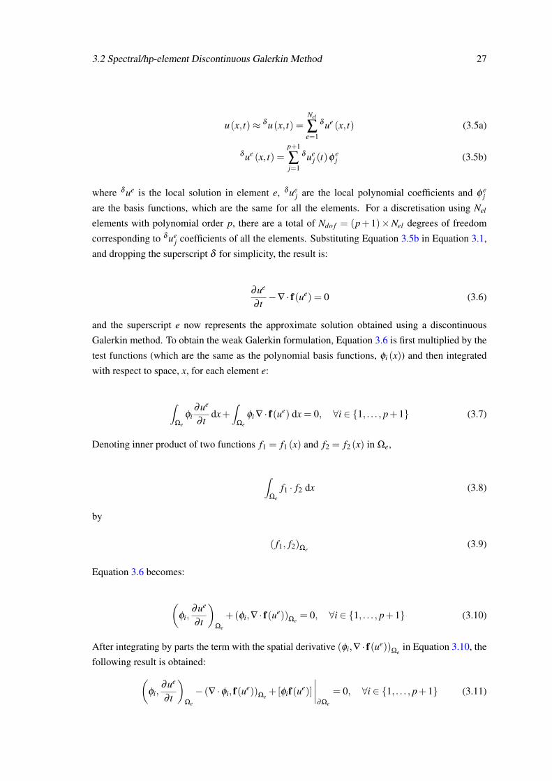
3.2 Spectral/hp-element Discontinuous Galerkin Method 27
u(x, t)≈ δ u(x, t) =Nel
∑e=1
δ ue (x, t) (3.5a)
δ ue (x, t) =p+1
∑j=1
δ uej (t)φ
ej (3.5b)
where δ ue is the local solution in element e, δ uej are the local polynomial coefficients and φ e
j
are the basis functions, which are the same for all the elements. For a discretisation using Nel
elements with polynomial order p, there are a total of Ndo f = (p+1)×Nel degrees of freedom
corresponding to δ uej coefficients of all the elements. Substituting Equation 3.5b in Equation 3.1,
and dropping the superscript δ for simplicity, the result is:
∂ue
∂ t−∇ · f(ue) = 0 (3.6)
and the superscript e now represents the approximate solution obtained using a discontinuous
Galerkin method. To obtain the weak Galerkin formulation, Equation 3.6 is first multiplied by the
test functions (which are the same as the polynomial basis functions, φi (x)) and then integrated
with respect to space, x, for each element e:
∫Ωe
φi∂ue
∂ tdx+
∫Ωe
φi ∇ · f(ue) dx = 0, ∀i ∈ 1, . . . , p+1 (3.7)
Denoting inner product of two functions f1 = f1 (x) and f2 = f2 (x) in Ωe,
∫Ωe
f1 · f2 dx (3.8)
by
( f1, f2)Ωe(3.9)
Equation 3.6 becomes:
(φi,
∂ue
∂ t
)Ωe
+(φi,∇ · f(ue))Ωe
= 0, ∀i ∈ 1, . . . , p+1 (3.10)
After integrating by parts the term with the spatial derivative (φi,∇ · f(ue))Ωe
in Equation 3.10, the
following result is obtained:(φi,
∂ue
∂ t
)Ωe
− (∇ ·φi, f(ue))Ωe
+[φif(ue)]
∣∣∣∣∂Ωe
= 0, ∀i ∈ 1, . . . , p+1 (3.11)
28 Numerical Modelling of Mooring Cables
The term in the square brackets [φif(ue)] in Equation 3.11 is the flux at the borders ∂Ωe of the
elements. In a discontinuous Galerkin method, this term is replaced by a numerical flux[φif(ue)
]and Equation 3.12 becomes:
(φi,
∂ue
∂ t
)Ωe
− (∇ ·φi, f(ue))Ωe
+[φif(ue)
]∣∣∣∣∂Ωe
= 0, ∀i ∈ 1, . . . , p+1 (3.12)
In the numerical model developed, the numerical flux applied used a modified version of the Local
Discontinuous Galerkin formulation [33], which will be described later in section 3.4. When the
term with the spatial derivative in Equation 3.12, (∇ ·φi, f(ue))Ωe
, is again integrated by parts, the
following result is obtained:
(φi,
∂ue
∂ t
)Ωe
+(φi,∇ · f(ue))Ωe
+[φi
( f(ue)− f(ue))]∣∣∣∣
∂Ωe
= 0, ∀i ∈ 1, . . . , p+1 (3.13)
Equation 3.13 represents the Green form of the Discontinuous Galerkin formulation [65], which
is the one that will be used for the numerical model. Each term in Equation 3.13 represents an
elemental matrix. For example, the first term,
(φi,
∂ue
∂ t
)Ωe
, ∀i ∈ 1, . . . , p+1 (3.14)
can be written as:
(φi,Φ
∂
∂ tue)
Ωe
, ∀i ∈ 1, . . . , p+1 (3.15)
where
Φ = [φ1 . . . φ j . . . φp+1] (3.16)
ue =[ue
1 . . . uej . . . ue
p+1]T (3.17)
and, by further rearranging the terms, expression 3.15, can be written as:
Me · ∂ ue
∂ t(3.18)
where
Mei j =
∫Ωe
φi (x)φ j (x) dx (3.19)

3.2 Spectral/hp-element Discontinuous Galerkin Method 29
is the entry i, j of the elemental matrix Me, also called elemental mass matrix (not to be con-
fused with mass matrices representing the inertia of physical systems). The elemental matrices
of the different elements are assembled in global matrices and the resulting system of ordinary
differential equations is then solved for the vector ue by matrix inversion.
As stated earlier, the discontinuous Galerkin formulation does not require the solution to be
continuous at the border of adjacent elements, as is represented in Figure 3.1. In fact, in Equa-
tions 3.10 to 3.13, there is no explicit coupling to the surrounding elements.
u
ue l
ue-1 r
ue+1 l
ue r
xe-1 r = xe
l xe r = xe+1
lx
Ω e-1 Ω e Ω e+1
Figure 3.1: Illustration of the variables in the spectral/hp-element discontinuous Galerkin method. Theindexes l and r indicate, respectively, the left and right borders of the elements.
The transfer of information between elements is achieved via the numerical flux f(ue). Using
the notation in Figure 3.1, the numerical fluxes at the borders of an element have, generally, the
form:
f(ue)|xel= fl
(ue
l ,ue−1r)
(3.20a)f(ue)|xer= fr
(ue
r ,ue+1l
)(3.20b)
where fl and fr are general functions indicating that the fluxes at the boundaries of element Ωe
might depend on the values of u at, respectively, the right and left borders of the surrounding
elements Ωe−1 and Ωe+1.
The application of boundary conditions will be described in section 3.4, for the specific case
of the numerical model developed, since they are applied through the numerical fluxes.

30 Numerical Modelling of Mooring Cables
3.3 Cable Dynamics
Figure 3.2 represents a section of a cable that has a mass per unit length ml and is under the
action of distributed external forces fext. A certain point on the cable has a constant lagragian
coordinate s, that is independent of the cable extension ε and of its current geometry. This
point is identified in a three-dimensional Cartesian reference frame Oxyz by its coordinate vec-
tor r(s, t) = (rx(s, t),ry(s, t),rz(s, t)). Along its length, the cable has an internal tension τττ (s, t),
with magnitude τ , that has the direction of the tangential vector t at every point, τττ = τ t.
x
y
zr(s,t)
tB
fext
s τBtA
τAA
B
Figure 3.2: Representation of the variables used to describe the dynamics of a cable.
For a cable with neither bending nor torsion stiffness, the equation of motion is [66, 67]:
∂ 2r∂ t2 =
1ml
∂τττ
∂ s+
1+ ε
mlfext (3.21)
The extension ε is determined using the following relation:
ε =
∥∥∥∥∂r∂ s
∥∥∥∥−1 (3.22)
Using Equation 3.22, the unit tangential vector t is given by
t =∂r∂ s
/
∥∥∥∥∂r∂ s
∥∥∥∥= 11+ ε
∂r∂ s
(3.23)
Equation 3.21 can also be written as:
∂ 2r∂ t2 =
1ml
∂
∂ s
(τ
1+ ε
∂r∂ s
)+
1+ ε
mlfext (3.24)

3.3 Cable Dynamics 31
The tension magnitude τ is determined using Hooke’s Law,
τ = EA0ε (3.25)
where E is the elasticity modulus and A0 is a nominal cross section of the cable. For the case of
a cable with constant cross section, A0 is its real cross-section. However, when the cross-section
varies, like in chains, A0 must be an equivalent value that can model the cable as if it had – in
what matters to elasticity calculations – a constant cross-section. In order to model hydrodynamic
forces and ground interactions, different values of the nominal cross section, as well as of the
diameter of the cable, will be required.
The vector fext of distributed external forces contains the contributions of weight, buoyancy,
hydrodynamic forces and ground forces. The submerged weight per unit length γl (which is the
net result of the buoyancy force and the weight) is given by:
γl =
(ρc−ρw
ρc
)mlg (3.26)
where ρc and ρw are, respectively, the density of the cable and of the water, and g is the acceleration
of gravity.
The hydrodynamic forces are accounted for using Morison’s formulations for added mass
force fm (Equation 3.27), tangential drag fdt (Equation 3.28) and normal drag fdn (Equation 3.29):
fm =Cm A1 (arel− (arel · t) t)(1+ ε) (3.27)
fdt =12
CdtρwD0 (vrel · t)2 t(1+ ε) (3.28)
fdn =12
CdnρwD0 ‖(vrel− (vrel · t) t)‖(vrel− (vrel · t) t)(1+ ε) (3.29)
where Cm, Cdt and Cdn are, respectively, the coefficients of mass, tangential drag and normal drag,
A1 is a nominal cross section of the cable, D0 is a nominal diameter of the cable and vrel and arel
are the relative velocity and acceleration between the cable and the water. The values of vrel and
arel are given by:
vrel = aw−∂r∂ t
(3.30)
arel = aw−∂ 2r∂ t2 (3.31)
where vw and aw are the water velocity and acceleration.
Similarly to the hydrodynamic forces, the ground forces are split between a component normal
to the ground and a component tangential to the ground. In the normal direction, the soil acts as
a bilinear spring-damper system. A stiffness force is applied to the cable when it is touching the
soil, and a damping force is applied to the cable when it is penetrating the soil, but not when it is

32 Numerical Modelling of Mooring Cables
being lifted [68, 69]:
fsn =
(KsD1∆H−2ζs
√KsD1 ml min(0,vsn)
)ns, if ∆H > 0
0, otherwise(3.32)
vsn =∂r∂ t·ns (3.33)
where fsn is the normal force, Ks is the bulk modulus of the soil, D1 is a nominal diameter of the
cable, ∆H is the normal penetration length in the soil, ζs is the soil’s damping factor and vsn is the
projection of the velocity of the cable in the direction normal to the soil, given by the unit vector
ns.
In the tangential direction, the soil applies a variable Coulomb friction force: when the tangen-
tial velocity of the cable is between zero and a limiting velocity vlim, the kinetic friction coefficient
is linearly ramped from 0 to its maximum value µs; when the tangential velocity is above vlim, the
kinetic friction coefficient is constant:
fst =−(
ρc−ρw
ρc
)mlg µs min
(‖vst‖vlim
,1)
ts (3.34)
vst =∂r∂ t− vsn ·ns (3.35)
ts =vst
‖vst‖(3.36)
where fst is the force applied by the soil on the cable in the tangential direction, g is the magnitude
of the acceleration of gravity and ts is the unit vector in the direction of the tangential velocity of
the cable.
3.4 Numerical Model
For the discretisation of the cable equation, the quantities length, time and mass per unit length
are made non-dimensional by scaling them with a characteristic length lc, time tc and mass mlc,
mlc = ml (3.37)
lc = l (3.38)
tc = l√
ml
τ0(1+ ε)(3.39)
where l is the unstretched length of the cable and τ0 is the pre-tension [70]. Using the symbol “ ˜ ”
to denote the non-dimensionalised variables, Equation 3.24 becomes:
∂ 2r∂ t2 =
∂
∂ s
(τ
1+ ε
∂ r∂ s
)+(1+ ε) fext (3.40)

3.4 Numerical Model 33
Following the procedure of [30] to write the cable equation as a system of two first order partial
differential equations in space, Equation 3.40 becomes:
∂ 2r∂ t2 =
∂
∂ s
(τ
1+ εq)+(1+ ε) fext (3.41a)
q =∂ r∂ s
(3.41b)
or, using Equation 3.21,
∂ 2r∂ t2 =
∂ τττ
∂ s+(1+ ε) fext (3.42a)
q =∂ r∂ s
(3.42b)
The exact solutions r and q are approximated by re and qe:
r(s)≈ re (s) = ∑ rej(t)
φ j (s) (3.43)
q(s)≈ qe (s) = ∑ qej(t)
φ j (s) (3.44)
where rej =(
rejx, r
ejy, r
ejz
)and qe
j =(
qejx, q
ejy, q
ejz
). The final discretised equations are:
(φi,
∂ 2re
∂ t2
)Ωe
=
(φi,
∂
∂ s
(τττ
e))Ωe
+[φi
( τττ
e− τττe)]∣∣∣∣
∂Ωe
+(
φi,(1+ ε) fext
)Ωe
, ∀i ∈ 1, . . . , p+1 (3.45a)
(φi, qe)Ωe
=
(φi,
∂ re
∂ s
)Ωe
+[φi
(re− re)]∣∣∣∣
∂Ωe
, ∀i ∈ 1, . . . , p+1 (3.45b)
As is usual for dynamic problems, the second order time derivative ∂ 2re/∂ t2 is integrated by steps:
instead of solving Equation 3.45a directly for the position re, the equation is first solved for the
acceleration ae, by setting
ae =∂ 2re
∂ t2 (3.46)
The acceleration is then integrated to velocity ve (which will be used in stabilising the numerical
model) and then to position re. Several different methods can be used for this procedure. In the
cases presented in sections 3.5 and 3.6, two different schemes were used: the Störmer-Verlet and
the Leap-frog method.

34 Numerical Modelling of Mooring Cables
The numerical fluxes were established using a modified version of the Local Discontinuous
Galerkin formulation [33]. Lets define the operators f and [[ f ]] as:
f (x)= 12( fl (x)+ fr (x)) (3.47)
[[ f (x)]] = fl (x)− fr (x) (3.48)
where, as in Figure 3.1, the indexes l and r are used to represent, respectively, the values of
function f to the left and to the right of border point x. Using this notation, the numerical fluxes
are expressed as:
re = re+κ [[re]] (3.49)τττ
e= τττe−κ
[[τττ
e]]+
λ1
h[[re]]+λ2h [[ve]] (3.50)
where κ ∈ [−1/2,1/2] controls the up- and down-winding of the fluxes (for centred fluxes, κ = 0),
λ1 and λ2 are constant, mesh independent parameters (the penalties) and h is the non-dimensional
element size.
The terms containing λ1 and λ2 in Equation 3.50 are used to provide stability to the method,
but the term containing λ2 is not part of the Local Discontinuous Galerkin formulation. It was
included here because it was found that it increased the robustness of the method, but it requires
further investigation. The velocity values ve are obtained as an intermediate step when determining
re, as explained above.
Evaluating the terms containing τττe requires special attention. The computed variables in the
numerical model are re and qe; τττe has to be determined as an intermediate step, once the values
of qe are known (see Equations 3.22, 3.25, 3.41a and 3.41b). Because of this, before computing
the fluxes, the approximation qe = ∑ q jφ j has to be computed in order to determine ε and then τe.
The value of τe (s) is then multiplied by qe = ∑ q j (t)φ j (s) to obtain τττe. The fluxes have to be
computed at the two boundaries of each element.
Boundary conditions are applied through the numerical fluxes. For a Dirichlet boundary con-
dition bD on a Dirichlet boundary ∂ΩeD and a Neumann boundary condition bN on a Neumann
boundary ∂ΩeN, the fluxes at the boundaries become:
re = bDτττ
e= τττ
e+
λ1
h
(re− bD
) on ∂ΩeD (3.51)
re = reτττ
e= bN
on ∂ΩeN (3.52)
3.5 Verification and Validation 35
3.5 Verification and Validation
3.5.1 Verification
Two test cases were selected to verify the properties of the numerical model. The first case is the
shape acquired by an elastic cable when hung between its two ends; the second case is a wave
propagating in a linear vibrating string. These two cases have analytical solutions that can be
compared with the results given by the numerical model. For both cases, the numerical solution
was obtained using different discretisations in the order p of Jacobi polynomials and in the element
size h. A measurement of the quality of the results of the numerical model is given by the L2 norm
of the error E :
‖E ‖L2 =
√∫Ω
(r− re)2 dΩ (3.53)
In the first case, a cable with an unstretched length of 100,5 m was fixed by its ends to points
100 m apart at the same height. Its stiffness was K = 200kN/m and its mass per unit length was
ml = 1,738kg/m. The penalty terms were set to λ1 = 5000 and λ2 = 0 and centred fluxes were
used (κ = 0). The solution to this case is provided by the equations of the elastic catenary [71]:
rx = aτsinh−1(
saτ
)+aτ
mlgK
s (3.54)
rz =√
a2τ + s2 +
mlg2K
s2−aτ (3.55)
aτ =τH
mlg(3.56)
where τH is the horizontal component of the tension force and rx and rz are the horizontal and
vertical component of the position vector r. The origins of the coordinate systems for r and s are
located at the lowest point of the cable. ‖E ‖L2 is presented in Figure 3.3.
For a reduced number of elements (only two), when the polynomial order p is increased, the
model shows the exponential convergence characteristic of p-type refinement, as demonstrated
by the straight line in the semi-logarithmic plot, Figure 3.3a. On the other hand, for constant
polynomial order, increasing the number of elements results in a much slower convergence to the
exact solution. Even with six times the degrees of freedom used in p-type refinement, the error in
h-type refinement is at least five orders of magnitude larger. This is the algebraic and sub-optimal
convergence of h-type refinement, demonstrated by the hyperbolic lines on the semi-logarithmic
plot and the straight lines on the logarithmic plot of Figure 3.3.
In the second case, the cable equation was linearised to have constant tension and extension,
both in time and along the whole length of the cable. In this situation, the partial differential
equation for the motion of the cable simplifies to the standard wave equation:

36 Numerical Modelling of Mooring Cables
0 50 100 15010
−10
10−5
100
L2−norm of the error for the static test.
Degrees of Freedom
L 2−no
rm o
f the
err
or
Nel
= 2, p = [1, 9]
Nel
= [2, 50], p = 1
Nel
= [2, 50], p = 2
(a) Semi-logarithmic plot.
101
102
10−10
10−5
100
L2−norm of the error for the static test.
Degrees of Freedom
L 2−no
rm o
f the
err
or
Nel
= 2, p = [1, 9]
Nel
= [2, 50], p = 1
Nel
= [2, 50], p = 2
(b) Logarithm plot.
Figure 3.3: L2 norm of the error, ‖E ‖L2 , in the simulation of the elastic catenary.
d2rdt2 =
τ
ml(1+ ε)
∂ 2r∂ s2 = c2 ∂ 2r
∂ s2 (3.57)
For this test, a 0,5 m cable was stretched to 1 m and fixed at both ends. Its mass per unit length
was 1 kg/m and its pre-tension was 1 N. The cable was initially deformed to have the shape of a
half-sine and then released. The solution to this case is given by Equation 3.58 [72]:
ry(s, t) = Acos(
cπ
L(1+ ε)t)
sin(
π
L(1+ ε)s)
(3.58)
where A is the amplitude of the sine, L is the stretched length of the cable and c is the transverse
wave celerity (Equation 3.57). A full oscillation cycle (2 s) was simulated using the leap-frog
scheme with a time step of 1×10⁻⁴ s, which was small enough to ensure that the error was domi-
nated by the spatial discretisation. Like for the static case, the penalties were set to λ1 = 5000 and
λ2 = 0 and centred fluxes were used (κ = 0). ‖E ‖L2 is presented in Figure 3.4.
As was the case for the elastic catenary, p-type refinement yields exponential convergence for
all the polynomial orders tested, as demonstrated by the straight lines in the semi-logarithmic plot.
Moreover, increasing the polynomial order provides such a fast convergence that ‖E ‖L2 reaches
the magnitude of the computer round-off error at around 10−11 and saturates. On the other hand,
increasing the number of elements for a polynomial order p = 1 (linear finite element method),
increases the number of degrees of freedom, but ‖E ‖L2 does not get anywhere near the computer
round-off error.
As expected, for smooth solutions, when the polynomial order is increased, the model exhibits
exponential convergence with a limited number of degrees of freedom, providing higher accuracy
solutions with less computational work when compared with the traditional formulation.

3.5 Verification and Validation 37
0 50 100 150 200 250
10−10
10−5
100
L2−norm of the error for the dynamic test.
Degrees of Freedom
L 2−no
rm o
f the
err
or
Nel
= 5, p = [1, 10]
Nel
= 10, p = [1, 10]
Nel
= 20, p = [1, 10]
Nel
= [1, 20], p = 1
(a) Semi-logarithmic plot.
101
102
10−10
10−5
100
L2−norm of the error for the dynamic test.
Degrees of Freedom
L 2−no
rm o
f the
err
or
Nel
= 5, p = [1, 10]
Nel
= 10, p = [1, 10]
Nel
= 20, p = [1, 10]
Nel
= [1, 20], p = 1
(b) Logarithm plot.
Figure 3.4: L2 norm of the error, ‖E ‖L2 , in the simulation of the vibrating string.
3.5.2 Validation
The results of the numerical model were validated against the data presented in [73], about exper-
iments on a submerged chain subjected to forced oscillations, Figure 3.5.
3,3 ± 0,003 m
32,554 ± 0,005 m
Motor with load cell
0,0 m
3,0 mChain 33 ± 0,005 m
Anchoring point
rm
Figure 3.5: Experimental set-up simulated to validate the numerical model.
A motor, installed above the water level, was used to drive the upper end of the chain in a
periodic circular motion with a radius of 0,20 m. At the connection to the motor, a load-cell was
installed to record the tension. Table 3.1 presents the values of the most relevant parameters of the
experimental set-up, as described in [73].
Two experimental cases were simulated using the numerical model: the chain being driven
with a period T = 3,50s and with a period T = 1,25s. The first case originated a slow motion of
the chain, which caused the tension to vary smoothly throughout the cycle, whereas the second
case originated quick motions that generated relative large and sharp peak loads.
The chain was modelled using 10 elements with Jacobi polynomials of order p = 1 to 7. The
penalty terms were set to λ1 = 5000 and λ2 = 1 and the fluxes were upwinded (κ = 1/2). Fifteen
consecutive cycles were simulated in order to achieve steady-state and investigate the numerical
dispersion. For time stepping a leap-frog scheme was used with a time-step of 1×10⁻⁴ s. The

38 Numerical Modelling of Mooring Cables
Table 3.1: Parameters of the experimental set-up.
Parameter Valuel (m) 33ρc (kg/m3) 7800ml (kg/m) 0,0818EA (N) 10000D0 = D1 = Link thickness (m) 0,0022Cm 3,8Cdt 0,5Cdn 2,5Ks (GPa/m) 3ζs 1µs 0,3vlim (m/s) 0,01ρw (kg/m3) 1000
portions of the chain that were above the water level were subjected to their dry weight and no
hydrodynamic forces.
The simulated tension forces at the top end of the chain are presented in Figures 3.6 and 3.7.
For both excitation periods, the measured and the simulated tensions are remarkably similar. The
shape of the tension cycle and the tension amplitude in the numerical simulations are close to
those obtained in the experiments. The model is even able to capture small details, such as the
indentation at the bottom and at the peak of the tension cycle for the excitation period of 1,25 s.
There is one notable difference between the simulated and the measured tension: the simulated
tension has a higher ripple content than the measured one and this is most evident when the tension
is close to zero. This phenomenon can have different origins, which are not fully understood. Part
of it can be explained by the digitisation of the experimental data, but it might also be caused by
the physics of the cable, by imperfections in the experimental set-up and or by numerical artefacts.
Probably, it is a combination of all, as explained below. High frequency oscillations in the tension
have been reported in experimental measurements [22, 24] and in numerical simulations [25],
although their cause was not explained.
The experimental data was obtained from digitisation of tension plots printed on paper. These
plots had ripple content, as do most experimental records (see, for example, Figure 5.17), which
was impossible to resolve in the scale at which the plots were printed. As such, those ripples could
not be digitised and the experimental tension looks smoother than it actually was.
If the ripples in the experimental data are due to the physics of the cable, then the numerical
model is able to capture fine details of the behaviour of the cable. If they are a result of imper-
fections in the experimental set-up, such as vibrations of the load cell or of the motor driving the
chain, noise in the data-logger, etc. then in the numerical results they are an artefact that must be
eliminated.

3.5 Verification and Validation 39
0 5 10 150
10
20
30
40
50
60
70
80
Tension for the excitation period of T=3,50s.
Time (s)
Ten
sion
(N
)
NumericalExperimental
Figure 3.6: Measured and simulated tension for the rotation period T = 3,50s.
0 5 10 150
10
20
30
40
50
60
70
80
Tension for the excitation period of T=1,25s.
Time (s)
Ten
sion
(N
)
NumericalExperimental
Figure 3.7: Measured and simulated tension for the rotation period T = 1,25s.

40 Numerical Modelling of Mooring Cables
The cable equation (Equation 3.24), which takes into account only axial stiffness, is a simpli-
fication of the dynamics of a real cable. This works well for cables under tension, but when the
tension is small or zero, the equation becomes singular, and the solutions undetermined [20, 21].
In this situation, small variations in the input data, together with computer round-off errors, cause
large variations in the solution and the resulting ripples. The penalty terms used in the numeri-
cal discretisation (λ1 and λ2) provide some robustness to the solution process by preventing the
right-hand term to become zero and by damping part of the ripples. A real cable has both bending
and torsional stiffness which, if included in the cable equation, would prevent it from becoming
singular. However, modelling such a cable results in a much more complicated equation, which
might not bring much added value when compared with its increased complexity.
It is known that modelling discontinuities using higher order functions may cause Gibbs-type
oscillations, as in the classical case of approximating a square wave with a Fourier series. This
might happen in the numerical model, since it uses high-order polynomials to approximate a so-
lution that is allowed to be discontinuous at the element boundaries. Additional discontinuities
are caused by shock loads: sharp and high amplitude tension peaks that occur when a slack cable
is violently re-tensioned. This is seen to happen for T = 1,25s, which presents a higher ripple
content than the simulation with T = 3,50s. To prevent this problem, numerical filters can be
applied to the numerical model to remove the ripples, although they were not applied in these
simulations. Even without any filtering, the ripple content is not too large and, for the excitation
period T = 3,50s, the ripples are not much larger than in the experimental records. Additionally,
in both simulations, the ripples die out quickly when the tension increases.
In these simulations it was also noticed that the results are sensitive to the ground parameters.
The ground model used was adopted from linear numerical models [68, 69] and might not be suit-
able for higher-order discretisations. This issue is further investigated and explained in [67] when
describing this same numerical model for cable dynamics: according to [15], in a dynamic simula-
tion where the cable interacts with the ground, shock waves might be generated at the points where
the cable impacts the ground and propagate along the cable. This effect was noticed to happen in
the numerical simulations. In lower order numerical models, with higher numerical dissipation,
these ripples are naturally damped. However, in this numerical model, with little dissipation, they
have little attenuation and require additional control measures, such as an improved ground model.
3.6 Moored Buoy Simulation
Since the aim of the numerical model developed is the simulation of moored floating wave energy
converters, the model was used to reproduce the physical model experiments of a moored buoy
presented in [74].
The experimental set-up, Figure 3.8, was composed of a cylindrical buoy in a wave tank,
moored on the seaward side by a chain and, on leeward side, by a horizontal nylon string connected
to a linear spring.

3.6 Moored Buoy Simulation 41
0,00 m- 0,21 m
0,90 m
Wave generatorBuoy
Chain
Nylon string
Spring
5,59 m
Figure 3.8: Experimental set-up reproduced in the simulation of the moored buoy.
Due to the design specifications imposed for the mass and for the inertia of the buoy, its
construction was rather complicated and resulted in a somewhat fragile hull, Figure 3.9.
Figure 3.9: Hull of the buoy, made of a stainless steel frame wrapped in a polyethylene sheet.
The properties of the buoy were determined experimentally following the procedures described
in [75] and are presented in Table 3.2.
Table 3.2: Properties of the model buoy. mb - mass; Db - diameter; Hb - height; ycg - position of the centreof gravity above the bottom of the buoy; db - draft; Icf - inertia around the horizontal axis through the centreof flotation.
mb Db Hb ycg db Icf
35,28 0,500 0,400 0,108 0,180 0,85±0,05kg ±0,002m ±0,002m ±0,004m ±0,008m ±0,03kgm2
The chain and the nylon string were attached at diametrically opposed sides of the buoy,
0,200 m above the bottom of the buoy and 0,020 m above the water level. A load cell was in-

42 Numerical Modelling of Mooring Cables
stalled in-line with the chain, at the connection of the chain to the buoy, to record the tension
force, Figure 3.10.
Figure 3.10: Placement of the load cell.
Long-crested regular waves with different heights, H, and periods, T , were generated in the
direction parallel to the the plane of the mooring cables. In these test conditions it is reasonable to
assume that the motion of the buoy was essentially two-dimensional and limited to surge, heave
and pitch.
The properties of the chain are listed in Table 3.3. The values of the axial stiffness EA and of
the hydrodynamic parameters were taken from [73] (such as in section 3.5.2) where a similar-sized
chain was used in physical model experiments. When in rest position, the tension in the chain (the
pre-tension) was 1,77 N.
Table 3.3: Properties of the chain.
Parameter ValueEA (N) (1,0±0,7)×104
ml(kg/m) (0,044±0,001)×10−4
γl(N/m) (0,382±0,006)×10−3
Outer link length (m) (16,6±0,7)×10−3
Outer link width (m) (7,1±0,7)×10−3
Link thickness (m) (1,7±0,5)×10−3
Cdt 0,5Cdn 2,5Cm 3,8
The nylon string had a negligible mass and the stiffness of the linear spring was 5,36 N/m.
The mass of the spring was judged to have little influence on the shape or in the tension of the
nylon string, since it was hung vertically above the water and the string was passed through a
pulley before being attached to the spring, Figure 3.8. When in rest position, the elongation of
the spring caused by the pre-tension of the nylon string was 0,243 m, yielding a pre-tension in the
string of 1,3 N.

3.6 Moored Buoy Simulation 43
An infra-red motion tracking system was used to record the rigid body motion of the buoy
in the six degrees of freedom and a resistive wave probe was used to measure the free surface
elevation two meters to the port side of the rest position of the buoy.
Out of the experimental test series, three conditions were chosen to be simulated: T = 1,30s,
H = 0,088m; T = 1,40s, H = 0,10m and T = 1,50s, H = 0,123m. Longer and higher waves
were not simulated as they had a pronounced second harmonic component; the shorter and smaller
waves were not simulated as the uncertainty in the recorded displacements was large. Neverthe-
less, the three conditions selected will be enough to illustrate some more characteristics of the
numerical model.
The buoy was modelled using linear potential theory, which, for a single excitation frequency,
describes the motions as a linearly damped oscillator [37]:
(M+A) ξξξ +B ξξξ +Cξξξ = fbuoy (3.59)
where A is the generalised mass matrix, A is the added mass matrix, B is the radiation damping
matrix, C is the hydrostatic stiffness matrix, ξξξ , ξξξ and ξξξ are, respectively, the acceleration, velocity
and position vectors in the six degrees of freedom and fbuoy is the vector of external forces acting
on the buoy (wave forces, mooring forces, etc.). Wave induced forces and moments are also
computed following linear potential theory:
fw = wη sin(
2π
Tt +δδδ
)(3.60)
where fw is the vector of wave induced forces on the buoy, w is the vector of the wave force
coefficients in the six degrees of freedom, η is the water surface elevation at the mean position of
the buoy and δδδ is the vector of the phase delay for each force and moment component.
Equation 3.59 was integrated in time using the Leap-frog scheme [76] with a time step ∆t =
1×10⁻² s. In reality, however, Equation 3.59 is only valid for floating structures subjected to
linear external forces, which is not the case for a buoy moored with a catenary. For time integra-
tion with non-linear external forces, Equation 3.59 should be replaced by Cummins’s formulation
[42]. Since the mass of the buoy was much larger than the mass of the mooring system, it was
assumed that the moored buoy had a weakly non-linear behaviour and, therefore, that it was valid
to represent it using Equation 3.59.
The hydrodynamic parameters of the buoy (added mass, radiation damping and wave force
coefficients) were determined using the formulation presented in [77] and are listed in Table 3.4.
Keeping with the assumption of a weakly non-linear behaviour of the buoy, viscous drag terms
were not included in the dynamics of the buoy.
The linear potential formulation used to determine the hydrodynamic coefficients assumes that
the water depth is constant, which was not the case in the experiments, Figure 3.8. Since the buoy

44 Numerical Modelling of Mooring Cables
Table 3.4: Hydrodynamic coefficients of the buoy.
T Mode Ai j Bi j wi δi (rad)
Surge 24,55 kg 31,73 kg/s 1057,8 N/m 1,475
1,30 sHeave 26,23 kg 37,94 kg/s 817,9 N/m 0,258
Pitch 0,2599 kgm2 0,03336 kgm2/s 34,30 N −1,667
Surge-Pitch 1,1739 kgm 1,0288 kgm/s - -
Surge 23,921 kg 20,82 kg/s 963,8 N/m 1,501
1,40 sHeave 27,05 kg 38,09 kg/s 921,8 N/m 0,206
Pitch 0,2581 kgm2 0,01974 kgm2/s 29,68 N −1,641
Surge-Pitch 1,1369 kgm 0,6410 kgm/s - -
Surge 23,17 kg 14,05 kg/s 880,2 N/m 1,519
1,50 sHeave 27,83 kg 37,47 kg/s 1016,4 N/m 0,168
Pitch 0,2564 kgm2 0,01213 kgm2/s 25,86 N −1,623
Surge-Pitch 1,1004 kgm 0,4129 kgm/s - -
is located at a point where the water depth is 0,900 m, this was the value used in the computation
of the hydrodynamic coefficients.
The leeward nylon string mooring leg was modelled as a simple linear spring with a pre-strain
of 0,243 m, that went slack when the strain was smaller than 0,000 m. The tension force of the
nylon string leg was applied to the buoy at a point 0,200 m above its bottom and at a distance of
0,250 m from its central axis. For simplicity, it was assumed that this force was always horizontal,
since the string had a negligible mass and, being taut, its angle to the horizontal at the connection
to the buoy was around 2.
The chain was discretised using 10 elements with 4th order Legendre polynomials (Ndo f = 50).
This discretisation was fine enough to provide grid independent simulations, as finer discretisations
using 5th and 6th order polynomials did not show significant differences in the results. Crossed
fluxes were used, meaning that the tension was up-winded and the position was down-winded, and
the stabilisation parameters were λ1 = λ2 = 1.
As cables cannot be compressed, the simulated chain had a bilinear stress-strain relation,
which allowed elongation, but did not allow compression. The values of the stiffness, mass and
drag coefficients used to model the chain are presented in Table 3.3. In the computation of the
hydrodynamic forces acting on the chain, the nominal diameters used were D0 = D1 = 0,0027m,
which is the diameter of a uniform cable made of the same material as the chain (steel, ρst =
7800kg/m3), that would have the same mass per unit length.
The anchoring point was set to a depth of 1,11 m, at a horizontal distance of 5,59 m from the
fairlead point when in rest position. The fairlead point was 0,2 m above the bottom of the buoy
at a distance of 0,250 m from its central axis. As most of the chain was hanging over the central
pit, the water depth used in the simulation of the dynamics of the chain was 1,11 m. This was also
the depth used for the computation of the wave length and of the wave induced water velocity and

3.6 Moored Buoy Simulation 45
acceleration. The difference in the water depth used to model the chain and to model the buoy
resulted in some additional discrepancies between the experimental and the simulated dynamics.
For the non-dimensionalisation, the characteristic length lc was the length of the chain, 5,88 m
and the characteristic time was 0,01233 s. The simulations were time-stepped using an explicit
Stormer-Verlet algorithm, with ∆t = 5×10⁻⁵ s for the wave periods T = 1,30s and T = 1,40s,
and ∆t = 2×10⁻⁵ s for the period T = 1,50s.
In order to control the numerical ripples seen in section 3.5.2, exponential filters were applied
to the position and to the tension in the chain, with each polynomial coefficient being multiplied
by a filter coefficient given by:
σ ( j) = exp
(−Γ
(j−Nc
p+1−Nc
)Λ), ∀ j ∈ 1, . . . , p+1 (3.61)
where σ ( j) is the filter coefficient applied to the polynomial coefficient j, Γ and Λ are parameters
that control the sharpness of the filter and Nc is the cut-off term of the filter (the filter has no effect
for j < Nc). This type of filter is described in [36]. In the simulations Nc was set to 0, Γ to 0,1 and
Λ to 10.
Coupling the simulation of the chain to the simulation of the buoy was achieved through a
special purpose function. At each time instant tn, the position pn of the attachment point of the
chain to the buoy was computed and transferred to the numerical model for cable dynamics. The
numerical model updated the previous position pn−1 of the upper end of the chain at time step tn−1
to the current position pn and computed the evolution of the tension between the two positions.
The tension at the current position and time τττn was then transferred to the linear potential theory
solver simulating the buoy. This new tension force was used by the linear solver, along with the
other loads, to determine the new position of the buoy and so on.
As the cable simulation requires a smaller time step than the simulation of the buoy, the nu-
merical model of the cable used linear interpolation to estimate the position of the top end of the
chain between the previous and the current position fed by the linear solver.
The characteristics used to model the ground are presented in Table 3.5. With the exception
of the limiting velocity vlim, they are the same as those used in subsection 3.5.2 since, in both
situations, the tank floor was made of concrete.
Table 3.5: Characteristics of the ground used in the simulation of the moored buoy.
Parameter ValueKs (GPa/m) 3ζs 1µs 0,3vlim (m/s) 1×10⁻⁴

46 Numerical Modelling of Mooring Cables
The tension at the upper end of the chain and the motion of buoy referred to the centre of
floatation are presented in Figures 3.11 to 3.13. Before analysing the results, it is important to
point out that both the numerical simulations and the experiments suffered from problems and
simplifications that affected the results. Some of these problems were detected only after the
experiments and the simulations had been carried out.
20 21 22 23 24 25 26 27−0.04
−0.02
0
0.02
0.04
0.06
0.08
0.1
Surge displacement H=0,088m, T=1,30s
Time (s)
ξ 1 (m
)
Experimental measurement Numerical simulation
(a) Surge
20 21 22 23 24 25 26 27
−0.05
0
0.05
Heave displacement H=0,088m, T=1,30s
Time (s)
ξ 3 (m
)
Experimental measurement Numerical simulation
(b) Heave
20 21 22 23 24 25 26 27−20
−15
−10
−5
0
5
10
15
20
Pitch displacement H=0,088m, T=1,30s
Time (s)
ξ 5 (°)
Experimental measurement Numerical simulation
(c) Pitch
20 21 22 23 24 25 26 270
2
4
6Experimental tension − H=0,088m, T=1,30s
Time (s)
τ (N
)
20 21 22 23 24 25 26 270
2
4
6Numerical tension − H=0,088m, T=1,30s
Time (s)
τ (N
)
(d) Tension
Figure 3.11: Comparison of experimental data and simulated results for regular waves with heightH = 0,088m and period T = 1,30s.
In surge, it is clear the existence of an offset in the mean oscillating position between the
numerical simulations and the experimental results. This offset is caused by second order drift
forces which, in the experiments, displaced the buoy from its rest position. Linear potential theory
takes into account only first order loads and no second order load. Therefore, the surge offset is
not due to any failure in the numerical model for cable dynamics.
On a deeper analysis of the results, it is seen that, for the three periods tested, the maximum
tension and the heave motions are well captured in the numerical simulations. The pitch and surge

3.6 Moored Buoy Simulation 47
20 21 22 23 24 25 26 27−0.04
−0.02
0
0.02
0.04
0.06
0.08
Surge displacement H=0,100m, T=1,40s
Time (s)
ξ 1 (m
)
Experimental measurement Numerical simulation
(a) Surge
20 21 22 23 24 25 26 27
−0.05
0
0.05
Heave displacement H=0,100m, T=1,40s
Time (s)
ξ 3 (m
)
Experimental measurement Numerical simulation
(b) Heave
20 21 22 23 24 25 26 27−20
−15
−10
−5
0
5
10
15
20
Pitch displacement H=0,100m, T=1,40s
Time (s)
ξ 5 (°)
Experimental measurement Numerical simulation
(c) Pitch
20 21 22 23 24 25 26 270
2
4
6Experimental tension − H=0,100m, T=1,40s
Time (s)
τ (N
)
20 21 22 23 24 25 26 270
2
4
6Numerical tension − H=0,100m, T=1,40s
Time (s)
τ (N
)
(d) Tension
Figure 3.12: Comparison of experimental data and simulated results for regular waves with heightH = 0,100m and period T = 1,40s.
motions (except for the surge offset) are well captured for T = 1,40s and T = 1,50s. For T =
1,30s, the pitch and surge motions are only reasonably captured, with the pitch amplitude being
larger than in the experiments, and the surge amplitude being smaller. The pitch resonance period
was estimated to be T = 1,19s in the experiments and T = 1,20s in the numerical simulations.
At T = 1,30s, the wave period is relatively close to the pitch resonance period, a situation where
linear potential theory is known to overestimate the motion amplitude (especially when viscous
damping is not modelled). As pitch and surge are coupled, this higher amplitude in pitch might
induce a smaller than expected amplitude in surge.
When it comes to tension, the amplitude of the numerical ripples is not as significant as in
the cases shown in subsection 3.5.2. Since the peak values of the tension are well captured, this
might mean that the filter applied is performing well and improving the results and the quality
of the numerical model. However, in contrast to the cases of subsection 3.5.2, the shape of the

48 Numerical Modelling of Mooring Cables
20 21 22 23 24 25 26 27−0.06
−0.04
−0.02
0
0.02
0.04
0.06
0.08
0.1
Surge displacement H=0,122m, T=1,50s
Time (s)
ξ 1 (m
)
Experimental measurement Numerical simulation
(a) Surge
20 21 22 23 24 25 26 27
−0.05
0
0.05
Heave displacement H=0,122m, T=1,50s
Time (s)
ξ 3 (m
)
Experimental measurement Numerical simulation
(b) Heave
20 21 22 23 24 25 26 27−20
−15
−10
−5
0
5
10
15
20
Pitch displacement H=0,122m, T=1,50s
Time (s)
ξ 5 (°)
Experimental measurement Numerical simulation
(c) Pitch
20 21 22 23 24 25 26 270
2
4
6Experimental tension − H=0,122m, T=1,50s
Time (s)
τ (N
)
20 21 22 23 24 25 26 270
2
4
6Numerical tension − H=0,122m, T=1,50s
Time (s)
τ (N
)
(d) Tension
Figure 3.13: Comparison of experimental data and simulated results for regular waves with heightH = 0,122m and period T = 1,50s.
tension cycle is not so well captured in these numerical simulations. The explanation for this is
not fully understood, but it might be partially related to the load cell used in the experiments.
Even though the load cell was submersible, it was not pressure compensated. This meant that the
water pressure around the cell reduced the tension readings. At rest, this effect was estimated to
reduce the measured tension by around 0,6 N to 0,8 N, but during the tests, the load cell moved
with the buoy and the water pressure was not constant. As such, during the tests, the pressure
effect was not constant, which might have changed the shape of the tension cycles. This does
not necessarily mean that the experimental maximum tension in the experiments was higher than
what was measured: the load cell could have been above the water level when the tension reached
its maximum value. Additionally, it was later found out that the load cell might have also been
somewhat damaged during the experiments.

3.7 Discussion 49
Another effect that may explain the difference between the measured and the recorded data is,
as mentioned earlier, the choice to integrate in time Equation 3.59 and 3.60 instead of Cummins’s
equation.
On a smaller scale, the fact that the numerical simulation could not account for the different
water depths in the experiments might cause some variations in the results as well.
3.7 Discussion
The numerical model showed a remarkable performance in the simulations presented. With rel-
atively few degrees of freedom, the maximum tension and the shape of tension cycle were well
determined. Even in long simulations, the solution did not show appreciable signs of numerical
dissipation or other integration errors that could build up with time. The only exception was the
simulation of the moored buoy in section 3.6, where the results were not as good as for the other
test cases. This particular test case was affected by the limitations of linear potential theory, used
to model the dynamics of the buoy, and by limitations in the experimental data, due to problems
with the sensors used in the physical model. Because of this, the results of this test case cannot be
expected to be fully representative of the quality of the numerical model. However, the numerical
model was still able to estimate correctly the peak tensions as measured in the physical model.
It was stated in [35] that the discontinuous Galerkin formulation can be expected to be better at
capturing shock waves than lower-order continuous methods. The ability of the model to correctly
estimate the peak tensions in the dynamic simulations (see sections 3.5.2 and 3.6), especially in
the cases with short oscillating periods, suggests that it might really perform well in this sense.
An important issue is the existence of high frequency ripples in the tension. The cause of these
ripples is not completely understood: they might be a physical phenomenon, or caused by limita-
tions in the experimental set-up or in the numerical model. The presence of ripples in experimental
measurements and numerical simulations of tension in cables has been known for some time, but
never fully explained [15, 22, 24, 25, 67]. As the numerical model uses a discontinuous formu-
lation, Gibbs oscillations might be generated at the boundary of adjacent elements. On the other
hand, the data acquisition interval of the load cells in the experiments (1×10⁻² s to 5×10⁻² s) is
much larger than the time-steps used in the simulations (1×10⁻⁴ s to 1×10⁻⁵ s). This might act
as a filter, smoothing ripples in experimental measurements.
The equation of perfectly flexible cables is known to be ill-posed when the tension is low.
Coincidently, the ripples are more prominent when the tension is low, which suggests a relation
between the two. If this is true, the ripples are not caused by the specific discretisation presented
here, but are due to the cable equation itself. In this case, the formulation will require stabilization
and filtering to attenuate this issue. The penalty term λ2 and the filter used in section 3.6 were
applied exactly with this purpose. The penalty term λ2, which can be compared to a damping
coefficient, is not a standard term in the Local Discontinuous Galerkin formulation. Although
beneficial in the simulations described, its effects on the numerical model and its optimization
require a deeper study. As explained in [67] the ripples might also be caused (or magnified) by

50 Numerical Modelling of Mooring Cables
the shock waves generated at the points where the cable impacts the ground, which was noted to
happen in the simulations presented. This phenomenon and its attenuation also require further
research. This ripple effect might be an evidence of the ability of the model to capture shock
waves. Shock waves are discontinuities in the solution and, as already mentioned, modelling
discontinuities with higher-order functions might cause Gibbs-type oscillations.
Finally, unlike lower order formulations, the time-step used in the test cases presented is rather
small (about 1×10⁻⁴ s to 1×10⁻⁵ s). Using such a small time-step in the numerical model might
counteract the gain in computational work from using fewer degrees of freedom when compared
with other formulations. The requirement to use small time-steps is a consequence of using ex-
plicit time-stepping schemes and higher order polynomials [35]: the maximum time-step allowed
decreases when either the polynomial order or the number of elements increase.
3.8 Conclusions
A numerical model for cable dynamics, which solves the partial differential equation of perfectly
flexible cables using the spectral/hp-element discontinuous Galerkin method, was developed and
presented.
It was demonstrated that the model has exponential convergence and that it can achieve high-
quality solutions with few degrees of freedom, a classical feature of higher order formulations.
The numerical model exhibited a remarkable performance in the reproduction of analytical and
experimental cases, where it determined accurate solutions and showed some ability to capture
shock loads. These features were targeted since the beginning of the development of the numerical
model, and are some of the reasons why a higher-order discontinuous Galerkin formulation was
used.
In the simulation of physical model tests of a moored buoy the results were not as good as
expected. However, the simulation of the moored buoy did not depend solely on the numerical
model for cable dynamics; it also depended on the simulation of the buoy itself, which was mod-
elled with linear potential theory. This theory has strong limitations in its range of application,
especially for periods near resonance. Furthermore, there were problems in the physical model
experiments and the experimental data might have a large uncertainty. As such, these simulations,
which were limited by the quality of the data they tried to reproduce, cannot be assumed to be
representative of the numerical model developed.
Further developments are required in the stabilization parameters and in the ground interaction
dynamics, in order to reduce numerical artefacts that stem from the low numerical dissipation of
high-order methods and from the Discontinuous Galerkin formulation.
Since the numerical model requires small time-steps (due to the use of explicit time-stepping
schemes together with higher order polynomials) part of the advantage of using few degrees of
freedom might be lost. This limitation should be overcome by the use of implicit time-stepping
schemes that allow the relaxation of the time-step requirements.

Chapter 4
Tracking Mooring Cables in PhysicalModels
4.1 Introduction
The tracking technique presented here measures the geometry of mooring cables in physical mod-
els, as when the moored object is excited by surface gravity waves, and has been described in
an earlier publication [78]. It processes underwater videos of the mooring cables, moving with
frequencies around those of the incident waves, and outputs the position of their medial axis.
Being thin and long elements, it is assumed that cables can be represented by their medial axis
without any impairment. When compared with other techniques, it has two major advantages: (i)
by capturing the complete medial axis of cables, it has no need for interpolation and (ii) all the
experimental steps are performed underwater, so it can be applied to a broad range of situations.
Since optics and image processing will play a major role in this task, a basic introduction to
some of their concepts is presented in section 4.2.
The physical model set-up used to test and develop the technique is described in section 4.3.
In the experimental phase of the technique standard photogrammetric methods, described in sec-
tion 4.4, are applied in order to obtain data to correct short-comings in the videos and acquire
essential parameters to convert the video data into physical values. Afterwards, a special-purpose
processing algorithm, described in section 4.5 interprets the videos and outputs the geometry of
the cable.
In section 4.6 it will be demonstrated that the technique is feasible and robust, performing
well even when contrast conditions are far from optimal. A basic error analysis is provided in
section 4.7 to show that, in spite of the prototype nature of this proof of concept, the error is
acceptable. As this work describes a proof of concept, it has not been optimised yet. Some
suggestions on further improvements are provided in sections 4.8 and 4.9.
The technique has only been tested using cables without floaters and sinkers. Furthermore,
because there was only one camera available, three-dimensional motion could not be determined,
51

52 Tracking Mooring Cables in Physical Models
so the technique is only demonstrated for cables with two dimensional motion. However, the de-
scribed procedures and algorithms can be easily expanded to determine three dimensional motions
if more than one camera is used.
4.2 Optical Concepts
An image can be interpreted as a scalar function of two variables or coordinates, u and v, which
are bounded by the dimensions of the image. Each point or pair of coordinates is assigned a
value which represents the intensity of light, I, at that point. In analogue images, the function is
continuous, but in a digital image the function is discrete. In the case of digital images, each point
in the image is called a pixel.
For black and white images, the intensity may take the value 0 for background pixels (usually
black) or 1 for foreground pixels (usually white). For 8 bit greyscale images, the intensity usually
takes integer values from 0 (black) to 255 (white) with the values in-between representing different
shades of grey. By specifying a colour map, the intensity values are converted into colours and the
image can be visualised.
Since a digital image is a function, it can be subjected to mathematical operations, some of
which will be described in the following text.
The optics of any imaging system are affected, more or less intensely, by some form of dis-
tortion, depending on its quality and purpose [59]. Two of these distortions (the most relevant for
this work) are the radial and the tangential distortion. These two kinds of distortion will have a
significant role in the experimental set-up, in the algorithm and in the error analysis.
Radial distortion may show up in two different ways: pincushion distortion, Figure 4.1 in
the centre, where the magnification increases radially from the centre of the image, and barrel
distortion, where the magnification decreases radially from the centre of the image, Figure 4.1 on
the right.
Figure 4.1: Representation of pincushion and barrel distortion on a square pattern.
4.2 Optical Concepts 53
Tangential distortion induces magnification that varies perpendicularly to the rays from the
image centre. This type of distortion is generally caused by the imperfect alignment of the different
optical components (decentering distortion) and comes associated with radial and other distortions
in a complex phenomenon [60].
Radial and tangential distortions are usually modelled using the Conrady-Brown polynomial
approximation [59, 60]. This model maps the position of the points in the distorted image to
the position of the points in the distortion-free image. The coefficients of the polynomial are the
distortion parameters of the camera and can be determined using different optimisation routines.
Usually, these routines consist of acquiring a series of photographs of a regular pattern with a
known geometry, and then estimating a fit of the polynomial that describes the distortion of the
pattern in the photographs. The distortion parameters, together with the focal length, the position
of the nodal points and the skewness of the image sensor are the intrinsic parameters of the camera.
An image whose optical distortions have been corrected is said to be linearised. Some of the
routines used to determine the intrinsic parameters are also able to determine the relative position
between the camera and the target in six degrees of freedom (orientation and position). These are
the extrinsic parameters of the camera.
If the images are captured underwater, the optical issues become more complex because the
lens is immersed in a fluid (air) with a different refractive index than that of the medium surround-
ing the object being imaged (water). Unless specific and expensive equipment is used, several
distortion artefacts will be added to the ones described above [62]. For example, the simple case
of using a standard camera through a transparent flat plane (a glass wall of an aquarium or the
glass of an under-water housing) will result in a reduced field of view of the camera, in the gen-
eration of pincushion distortion and in an image with multiple focus points [62, 64]. Part of these
problems can be fixed using a hemispherical dome port between the lens and the water, instead
of a flat one. This preserves the field of view of the camera and maintains a single focus point
[62]. The downside of using a hemispherical dome port is that the image created will be a curved
surface instead of a flat plane, as in most cameras. In order to have the entire image surface in
focus, the depth of field (the thickness of the volume seen by the camera that is in focus) has to be
large enough to encompass the depth of the surface. For a lens with a constant focal distance, this
usually means that the aperture has to be reduced. A full mathematical description of this problem
is given in [62].
Another problem arising when imaging underwater is that, in general, the linearisation proce-
dures mentioned earlier are not valid. The Conrady-Brown model for correcting optical distortions
was developed for cameras in air imaging subjects that are also in air, where the linearisation is
valid for any camera-to-object distance and for different focus adjustments [63]. Special (and
rather complex) procedures are required for underwater linearisation, an area which still requires
some development. Under certain conditions, however, the in-air linearisation procedure can be
applied underwater. For this to be valid, the linearisation must be performed underwater for the
specific distance between the camera and the object of interest, and the optical characteristics of

54 Tracking Mooring Cables in Physical Models
the camera cannot be altered after linearisation. The restrictions mentioned above were adopted in
the experimental set-up described later, so the in-air linearisation method could be used.
Since a photograph is a projection of a three dimensional object onto a plane, the result of the
projection depends on the relative position between the camera and the object, Figure 4.2. The
apparent change of shape of the object with change of the view point is known as keystone effect
and is caused by the viewing axis not being perpendicular to the plane or planes captured in the
image.
Figure 4.2: Keystone effect. When a face of an object is projected onto an oblique plane, the shapes in theresulting projection are not geometrically similar to the ones in the object.
The keystone effect can be partially corrected using an operation called homography. This oper-
ation takes the original image and re-projects it onto another plane [79, 80]. By re-projecting the
photograph in a plane parallel to the one affected by the keystone effect, the effect is partially elim-
inated. Evidently, after applying an homography transformation, the keystone effect might appear
in other objects in the image that are now viewed from an oblique angle and, hence, it might be
impossible to correct this effect in the entire image at once. This operation is a simple matrix
multiplication that requires only the intrinsic parameters of the camera, as well as the current and
the desired orientation of the projection planes. When an image is corrected so that the real object
and the object in the image have geometric similarity, the image is said to be rectified.
Accurate measurements using imaging techniques require geometric similarity between the
object and its representation, implying that all of the distortions and optical effects be corrected.
Once these effects are corrected, the use of an appropriate linear transformation should (ideally)
convert the positions of the points of the image to coordinates in the desired reference frame. The
image is then said to be calibrated. Calibration might be as simple as the multiplication of each of
the coordinates of the points in the image by a constant.
Besides correcting optical artefacts, images can be subjected to another type of transforma-
tions: morphological operations. For this work, the most relevant are dilation, thinning, edge-
detection and the top-hat transform .

4.2 Optical Concepts 55
Dilation enlarges objects or shapes by super-imposing on foreground pixels a specified shape,
called structuring element, Figure 4.3. The structuring element has an origin which is matched to
each foreground pixel when adding the two shapes together, Figure 4.3.
Initial shape Structuring element Dilated shape
Origin
Figure 4.3: Dilation. The origin of the structuring element (marked with×) is matched to each of the pixelsin the initial shape (marked with ) and its pixels added together, resulting in the dilated shape.
Thinning is an operation that shrinks shapes by reducing their thickness by one or two pixels
[81]. When executed several times, thinning will reduce objects to simple strokes, but it will never
break the object or make it disappear, Figure 4.4.
Initial shape Thinning appliedonce
Thinning appliedrepeatedly
Figure 4.4: Thinning. Successively reducing the thickness of a shape will result in a one-pixel wide strokethat is approximately the medial axis of the shape.
For a simple shape, the remaining stroke after thinning has been applied several times is ap-
proximately the medial axis of the shape. Contrary to dilation, thinning does not require a struc-
turing element.
Edge detection looks for regions in greyscale images with large gradients in the intensity values
[81]. These regions usually correspond to edges of the objects in the image, but may also be
generated by shadows, differences in illumination and other perturbations.
The top-hat transform detects the bright regions in an image that are narrower than a selected
structuring element or, in simpler terms, regions where the structuring element cannot fit in, Fig-
ure 4.5. When an image, such as Figure 4.5a is represented as three-dimensional plot, Figure 4.5b,
the brighter regions will appear as peaks and plateaus, while the darker regions will appear as
valleys. Some of the bright regions, like the sharp peak on the right of Figure 4.5c, are narrower
than the structuring element, which in this case is a simple 3 pixel wide cross. These regions
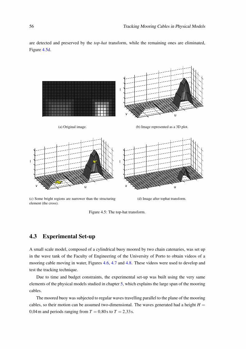
56 Tracking Mooring Cables in Physical Models
are detected and preserved by the top-hat transform, while the remaining ones are eliminated,
Figure 4.5d.
(a) Original image. (b) Image represented as a 3D plot.
(c) Some bright regions are narrower than the structuringelement (the cross).
(d) Image after tophat transform.
Figure 4.5: The top-hat transform.
4.3 Experimental Set-up
A small scale model, composed of a cylindrical buoy moored by two chain catenaries, was set up
in the wave tank of the Faculty of Engineering of the University of Porto to obtain videos of a
mooring cable moving in water, Figures 4.6, 4.7 and 4.8. These videos were used to develop and
test the tracking technique.
Due to time and budget constraints, the experimental set-up was built using the very same
elements of the physical models studied in chapter 5, which explains the large span of the mooring
cables.
The moored buoy was subjected to regular waves travelling parallel to the plane of the mooring
cables, so their motion can be assumed two-dimensional. The waves generated had a height H =
0,04m and periods ranging from T = 0,80s to T = 2,33s.
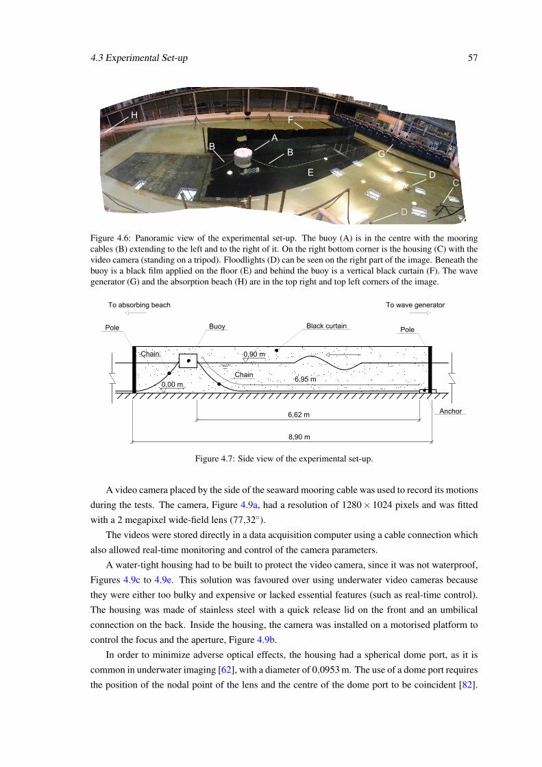
4.3 Experimental Set-up 57
C
A
B G
D
D
H
B
E
F
Figure 4.6: Panoramic view of the experimental set-up. The buoy (A) is in the centre with the mooringcables (B) extending to the left and to the right of it. On the right bottom corner is the housing (C) with thevideo camera (standing on a tripod). Floodlights (D) can be seen on the right part of the image. Beneath thebuoy is a black film applied on the floor (E) and behind the buoy is a vertical black curtain (F). The wavegenerator (G) and the absorption beach (H) are in the top right and top left corners of the image.
Figure 4.7: Side view of the experimental set-up.
A video camera placed by the side of the seaward mooring cable was used to record its motions
during the tests. The camera, Figure 4.9a, had a resolution of 1280× 1024 pixels and was fitted
with a 2 megapixel wide-field lens (77,32).
The videos were stored directly in a data acquisition computer using a cable connection which
also allowed real-time monitoring and control of the camera parameters.
A water-tight housing had to be built to protect the video camera, since it was not waterproof,
Figures 4.9c to 4.9e. This solution was favoured over using underwater video cameras because
they were either too bulky and expensive or lacked essential features (such as real-time control).
The housing was made of stainless steel with a quick release lid on the front and an umbilical
connection on the back. Inside the housing, the camera was installed on a motorised platform to
control the focus and the aperture, Figure 4.9b.
In order to minimize adverse optical effects, the housing had a spherical dome port, as it is
common in underwater imaging [62], with a diameter of 0,0953 m. The use of a dome port requires
the position of the nodal point of the lens and the centre of the dome port to be coincident [82].

58 Tracking Mooring Cables in Physical Models
Figure 4.8: Top view of the experimental set-up.
Guiding pins on the lid of the housing ensured that the dome port would maintain its alignment
with the camera even when the lid had to be removed. Despite the effort in designing the housing,
neither the dome port could be provided in optical quality glass nor a perfect positioning of the
camera could be guaranteed with the equipment available. As a consequence, there is a small
distortion in the videos that could not be corrected using theoretical models.
To keep in focus all of the curved image generated by the dome port, the aperture of the camera
was set to a low value, maximising the depth-of-field. Because of the reduced aperture, together
with water quality issues, the recorded images had a somewhat low quality.
The simpler flat port was rejected because of the problems mentioned in section 4.2, which
cannot be easily corrected. Additionally, earlier tests using a flat port demonstrated that it would
be unsuitable because of the reduced field of view. This is illustrated in Figure 4.10, showing a
photograph of a catenary with the same camera used in these experiments, but taken through a flat
port. Although the cable spanned only 5,59 m, it was not possible to capture its whole length.
To capture the entire span of the seaward mooring chain, the camera had to be positioned
4,29 m away from the model, Figure 4.8. Since the floor and walls of the tank were light beige

4.3 Experimental Set-up 59
(a) Video camera. (b) Motorised control system.
(c) Underwater camera housing viewed from the side. (d) Fully assembled imaging system viewed fromthe front.
(e) Fully assembled imaging system viewed from theside
Figure 4.9: Components of the imaging system used to record the motions of the cables.

60 Tracking Mooring Cables in Physical Models
Figure 4.10: Photograph of a mooring cable taken through a flat port. The water depth is 0,900 m and thespan of the cable is 5,59 m. The small field of view caused by the flat port of the housing made it impossibleto capture the entire length of the cable. Pincushion distortion is also visible in the image, causing the edgesof the pit to appear curved.
and the chain was silver grey, it was difficult to distinguish both from afar when under water.
In addition, the tank water had a high content of suspended material (dust and minerals), which
absorbed and scattered light. This problem could be so intense that, at times, it would completely
hinder the acquisition of any video during the experiments. The large thickness of water between
the camera and the cable, combined with the visibility problems, resulted in images with somewhat
low contrast, Figure 4.11.
Figure 4.11: Underwater photograph of the cable with minimal contrast enhancement, showing a foggyhaze caused by the suspended dirt in the water of the wave tank.
In order to improve contrast, the chain was brightened and the background was darkened. This
solution was chosen for practical reasons: most wave tanks have dark walls (due either to con-
struction or to dirt) and it is easier to make a small cable brighter so it stands out against a dark
background, than to brighten the whole inside of a wave tank. A dark cable on a light background
might even result in the cable fading in the image due to light scattering and to saturation of the
image sensor in the video camera.
A coat of white paint was applied to the chain, which was also illuminated with four underwa-
ter floodlights placed along its length, distributing the light evenly, Figures 4.6 and 4.8. The use

4.3 Experimental Set-up 61
of cheaper and simpler flood lights pointing downward to chain from above the water was tried in
preliminary tests, but it caused severe saturation of the imaging sensor, Figure 4.12
Figure 4.12: Saturation of the image caused by vertical light reflecting off the floor (on the left). Thesaturated region blocks the visibility of the portion of the chain near the corner of the pit.
Beneath the chain, the tank floor was covered with a black sticker film which had a matte
surface, in order to minimise light reflections, Figures 4.6 to 4.8. Red markings were placed every
0,500 m on the black film in the direction of the cable starting at the anchoring point, to be used
as references.
Behind the chain, a black curtain was hung between two poles, aligned with the wave direction,
Figures 4.6 to 4.8. Imposing the use of a curtain would severely limit the range of application of
the technique: for example, in multi-directional sea-states, a shadow region would be created.
However, it will be shown in section 4.6 that the technique is fully functional when the vertical
curtain is removed, which will be a requirement in most situations. In these experiments it was
only used to improve the contrast conditions and the video quality for the development of the
technique.
In spite of the seemingly elementary approach to improve contrast, it was the most effective
one from all of the tested solutions. Besides what was described above, two other solutions were
tried. In one of them, electroluminescent cables were threaded through the links of the chain, but
they were too stiff and too large. In the other, ultra-violet light (UV) was used to illuminate the
chain, which was painted with fluorescent and phosphorescent paint. The UV light should induce
the fluorescence and phosphorescence of the paint in the chain and, being invisible to the camera,
UV would not cause saturation. However, the power of the ultra-violet lights available was too
weak to excite the paints and any light emitted by the chain was too faint to be useful.
Independently of the conditions in the used laboratory, it is always necessary to assure that the
cables stand-out well enough to be detected by the processing software. This will usually result
in the need to enhance contrast. Even though this might seem trivial, it is worth to emphasise
it because, at least at the present moment, a feasible processing algorithm is very limited when
compared to the human ability to interpret images.
It is important to remember that contrast in the experimental set-up is obtained by making the
cable lighter than the surroundings, because the processing algorithm described later is designed
to look for small bright regions in the images.

62 Tracking Mooring Cables in Physical Models
In some steps of the tracking technique described in the next section, namely for the linearisa-
tion and for the calibration, a flat target with a chess-like pattern will be required. The target that
was used in this work is shown in Figure 4.13.
(a)
(b)
Figure 4.13: Target used for the experimental steps of linearisation and calibration.
It was made of a square pattern printed on a white plastic film pinned to a chipboard panel. On its
back it had metal supports to keep it vertical when placed on the floor.
For the procedures involving image processing and algorithm coding, the software suite MAT-
LAB was used. Even though it is a proprietary software and relatively slow when compared to
other programming languages, it provided a reasonable platform for prototyping. All efforts were
made to use solely standard image processing functions, instead of any function exclusive to MAT-
LAB, so that the algorithm developed could be programmed and tested in different environments.
The special purpose “Camera Calibration Toolbox For MATLAB” [83] that will be used in some
steps of the technique, as well as its source code, are freely available and can be fully inspected.
4.4 Tracking Technique - Experimental Procedure
Three different steps are required in the experimental phase: (i) linearisation, to obtain the intrinsic
parameters of the camera required to correct the optical distortions; (ii) calibration, to obtain the
relative position between the camera and the cable (the extrinsic parameters) and the correspon-
dence between pixel and model coordinates, respectively; and (iii) video acquisition of the cables
moving underwater.
Linearisation is a conditional step: it is only required if the camera is not designed to provide
distortion-free images underwater or if the optical parameters of the camera are not known. The
video camera used in the experiments distorts the images when it is used underwater so linearisa-
tion was a necessary step.
For the linearisation, the freely available Camera Calibration Toolbox for Matlab [83] was
used. This toolbox is based on the Conrady-Brown distortion model [59, 60], see section 4.2,
which, in general, is not valid when either the camera or the object being imaged are submerged.
However, as noted by [64], the Conrady-Brown model may be applied underwater (and, in fact,

4.4 Tracking Technique - Experimental Procedure 63
it frequently is) with some constraints: its application will be limited to a single camera-to-object
distance. As an example, in the set-up used in these experiments, Figure 4.8, moving the camera
sideways would not require a new linearisation, but moving the camera towards the cable would.
During linearisation, the target in Figure 4.13 is photographed in several positions in the plane
of the seaward mooring cable along its span, Figure 4.14.
Figure 4.14: Examples of some photographs of the target during linearisation, in different orientations andpositions along the plane of the cable.
Table 4.1 presents the intrinsic parameters of the imaging system used in the experiments,
obtained after linearisation using the Conrady-Brown model. Following the recommendations
of the toolbox user’s manual, the coefficients were estimated only up to 4th order; higher orders
should not be used when the error in the coefficients is similar to the coefficients’ magnitude. In
the same way, the skewness of the camera sensor was not estimated as it was almost 90, as is
usual in modern, high quality cameras.

64 Tracking Mooring Cables in Physical Models
Table 4.1: Intrinsic parameters of the imaging system.
Parameter x direction y direction Skew ()
Focal length (pixel) 841±24 838±24 0
Image centre (pixel) 607±21 554±25
Distortion coefficients
1st order 2nd order 3rd order 4th order
(−8,7±2,8)×10−2 (9,5±4,1)×10−1 (9,6±6,8)×10−3 (2,5±6,6)×10−3
Although the fitted polynomial was limited to 4th order, the error in the coefficients was still
significant. This is probably due to the limitations of the video system caused by the quality of the
dome port and by the inaccuracy in centring the dome and the lens of the camera.
4.4.1 Calibration
This step determines the transformation required to correct the keystone effect (see Figure 4.2)
and to convert pixel coordinates to the desired model coordinates.
To acquire the calibration data, the target in Figure 4.13 is positioned in the plane of the cable
in a known location, as shown in Figure 4.15. The target should not be tilted in any direction in
relation to plane of the cable, so (in these experiments) it was held in place by the metal supports
on its back. A single photograph is taken of the target in this position.
Figure 4.15: Position of the target during the calibration phase.
Knowing the intrinsic parameters of the imaging system, the distortions in the image are cor-
rected. Then, the current orientation of the local reference frame of the target (O xt yt zt) relative
to the camera (the extrinsic parameters), are determined, Figure 4.16. Both of these steps are
executed using the “Camera Calibration Toolbox for MATLAB”.
Once the current extrinsic parameters are known, a new matrix of extrinsic parameters is built
defining an orientation where the target is parallel to the imaging plane (in other words, where

4.4 Tracking Technique - Experimental Procedure 65
Figure 4.16: Local reference frame of the calibration target as established by the “Camera CalibrationToolbox for MATLAB”. The zt axis is not shown because it is almost perpendicular to the photograph.
the zt axis is aligned with the camera viewing axis). This matrix is then used in the homography
transformation to obtain the desired new orientation of the plane of the image. The local xt and
yt axes do not need to be rotated, but they were anyway so that, for convenience, the images are
properly oriented when displayed.
In the rectified image, four points are selected whose coordinates in the model are known, as
illustrated in Figure 4.17.
B
A
C
D
Figure 4.17: Points used for the calibration of the experimental set-up.
By defining a model coordinate frame (0 xm ym zm) with the origin at the anchoring point, the
xm axis pointing to the left and the ym axis pointing up, the coordinates of the points A, B, C and
D in Figure 4.17 are established, Table 4.2. Inspecting Figure 4.17, the pixel coordinates of points
A,B,C and D can also be determined. Then, a multivariate least-squares fit is used to compute
the matrix that converts pixel to model coordinates. To minimize the conversion error, the points
should be spread across the entire measurement region, but not aligned.
Image rectification and calibration could be merged into a single step, which would both sim-
plify the procedure and make the Camera Calibration Toolbox for MATLAB necessary only for
linearisation (if necessary at all). However, the technique is just a proof-of-concept and the extra

66 Tracking Mooring Cables in Physical Models
Table 4.2: Coordinates of the calibration points in the model reference frame.
Point Coordinates
A (6,500;0,000)m
B (4,000;0,599)m
C (3,231;0,599)m
D (0,000;0,000)m
work demanded to merge rectification and calibration would not bring any new development or
significant advantage at this stage.
The calibration is obviously dependent on the relative position and orientation between the
camera and the cable.
4.4.2 Video Acquisition
Video acquisition (the recording of the motions of the cable) is the last experimental step. As
the objective of the technique is to detect the geometry of cables as a function of time, the video
specifications, namely the frame rate and the resolution, are of utmost importance.
The frame-rate is the acquisition frequency of the video camera. Just like for general data
acquisition [84], it must be at least twice that of the highest frequency phenomena with a noticeable
contribution to the shape of the cable.
The video resolution will determine the smallest dimension or detail that can be detected
by the camera. Any physical characteristic or motion that, when viewed from the camera, is
smaller than the width of a pixel, will be imaged together with its surroundings and will become
undistinguishable. The size d of the details contained in each pixel is obtained by the simple
equation:
d =Lt
Np(4.1)
where Lt is the total length covered in a certain direction and Np is the number pixels in the length
Lt . For instance, in the set-up used in this work, the horizontal field of view encompasses 8,90 m
(including the regions to the left and to the right of the cable), Figure 4.7. Since the camera has
a horizontal resolution of 1280 pixels, the resolution for this set-up is 0,007m/pixel and no detail
smaller than 0,007 m will be detected. To obtain finer resolutions, either the camera has to be
placed closer to the cable or a camera with a higher resolution has to be used.
In practice, the minimum requirements for the frame rate and resolution only guarantee that
the motions are detected, but not that their detailed evolution in time and space are appropriately
captured. As such, the resolution and the frame rate should be well above the minimum values,
in order to capture the behaviour with enough detail. Perturbations in the data acquisition, such
as poor visibility or other interferences, will also demand the use higher data acquisition rates.

4.5 Tracking Technique - Processing Algorithm 67
Additionally, the values of the frame rate and resolution are interdependent. They must be such
that it is possible to record a change of shape or position with a specified magnitude in the time
span between two frames. An example would be the need to capture the propagation of a transverse
wave along the cable with variations in the displacement no larger than 0,001 m with a time-step
no larger than 0,01 s.
For the experiments described in this chapter, the frame-rate was 15 frames per second (15 Hz).
The frame-rate is considerably low when compared with usual acquisition frequencies in coastal
engineering models (around 100 Hz). This low value was chosen because the file size of the
videos grows rapidly with the frame-rate and, for this proof of concept, a large frame-rate was not
required.
As stated in the Introduction, all the experimental steps (linearisation, calibration and video
acquisition) are executed underwater, without any need for side windows in the tank or other
access constraints.
4.5 Tracking Technique - Processing Algorithm
The algorithm will be explained using a worked example. For this, a small clip was extracted from
a larger video. In this clip, the waves have a height H = 0,04m and a period T = 1,14s.
The wave period is close to the resonance period of the moored buoy in heave (T = 1,13s)
and pitch (T = 1,16s) in order to induce extreme velocities and displacements on the cable. To
skip the ramping sequence of the wave generator (when the waves are small and vary in size), the
clip begins with the cable in a non-stationary position, Figure 4.18, subjected to fully developed
regular waves.
Figure 4.18: First frame of the processed clip, after correcting the distortion and the keystone effect. Thecable is not in static equilibrium, because the clip was extracted from a longer video. The image histogramhas been modified to enhance visibility when printed.
Before processing the video, the user estimates, by inspection, the maximum expected dis-
placement (in pixels) of the cable between two successive frames. This information is important
because it will be used by the algorithm to determine where in the image to search for the cable as
it moves from frame to frame, as well as to remove unwanted features.

68 Tracking Mooring Cables in Physical Models
The first frame of the video is extracted and the distortion and perspective effects are corrected,
Figure 4.18. Note the dull or foggy appearance of the image caused by the suspended dust in the
water.
Even though a person can clearly identify the cable when looking at Figure 4.18, the algorithm
is unable to do so without assistance. To this end, a search region is manually defined around the
cable, Figure 4.19, which should be as tight as possible without intersecting the cable.
Figure 4.19: Initial search region (enclosed by the white contour) provided to the algorithm to assist in thedetection the cable. The image histogram has been modified to enhance visibility when printed.
This region is stored as a mask, a logical matrix with the same dimensions as the image with entries
that take the value 1 in positions corresponding to the search region and the value 0 everywhere
else.
From now on, all processing will occur inside the search region, disregarding the rest of the
image. The use of a search region not only speeds up the algorithm, because there is less data to
process, but also and more importantly, limits the area where the algorithm can look for the cable,
reducing the possibility of detecting unwanted features.
The search region is defined manually only for this first frame, just for the algorithm to have a
starting point. Afterwards, the algorithm will use the medial axis of the cable in the current frame
and the maximum expected displacement between two frames to automatically update the search
region as the cable moves.
Selecting the search region can be compared to designating the set of markers that are to be
tracked in conventional motion-capture technologies. If the experimental set-up is not altered,
including the position of the camera, the search region has to be delimited only once and can then
be used for the entire series of tests.
Once the search region is defined, the cable has to be separated from the background of the
image. Since the cable is brighter than the background, the top-hat transform is applied to separate
the image of the cable from the background, using a circular structuring element, Figure 4.20. The
diameter of this structuring element (in pixels) should be equal to the average thickness of the
cable in the image, which must be determined by visual inspection (for example, when defining
the initial search region). It is important that the diameter of the structuring element is as close
as possible to the thickness of the cable: if the diameter is too large, unwanted features might be
detected and if the diameter is too small, the cable might not be completely detected.
In the images, the cable can be recognised by a being bright, long and thin shape. Therefore,
an edge detector will efficiently trace its outline. For this, the Canny edge detector was used. This

4.5 Tracking Technique - Processing Algorithm 69
Figure 4.20: The result of applying the top hat transform to the search region. Contrast has been enhancedover the entire image so that the result of the top-hat transform is clear, because this transform lowers theintensity of the processed regions.
edge detector can detect edges in several directions, even in images where the edge sharpness is
poor [81], such as in photographs with motion blur.
The result of applying the Canny edge detector is shown in Figure 4.21, where all the data on
and outside of the border of the search region was deleted.
Figure 4.21: The result of applying the Canny edged detector: the outline of the cable is efficiently traced.
The outline of the cable is clear and sharp, but the process is not yet complete: the cable is
represented by its outline instead of its medial axis and there are small extraneous streaks around
the cable, as in Figure 4.22.
Figure 4.22: Example of an extraneous streak that will interfere in the detection of the cable. These streaksare caused by the application of the Canny edged detector. This image is taken from a later portion of theclip to illustrate this problem.
Analysing Figure 4.22, one can see that the small streaks are not longer than the width of
search region. They cannot be longer because their size is limited by the search region. If the
initial search region is tight enough around the cable, the maximum width of the search region
in any subsequent frame is twice the maximum expected displacement (the cable can move to
either side of its current position). With this in mind, all streaks shorter than twice the maximum
expected displacement are deleted. Any extraneous streaks that might happen to be connected to
the cable cannot be removed at this stage.

70 Tracking Mooring Cables in Physical Models
In order to fill in the outline of the cable and connect any loose segments, the image is dilated
using a circular structuring element with a radius equal to half of the thickness of the cable, Fig-
ure 4.23. This is the smallest radius which ensures that the opposite edges are joined together.
As such, this radius minimises the risk of distorting the geometry by merging together sections of
the cable that are momentarily next to each other in the image, even though they belong to distant
parts of the cable.
Figure 4.23: Outline of the cable filled in using dilation.
After filling in the outline, the cable is thinned until stability is achieved. This method was
used in [58] to determine the camber of steel slabs. The result is the medial axis of the cable, with
any existing extraneous branches still attached. These branches can now be removed. First, the
branch points are detected and a small circular area around them is erased, breaking the branches
apart. The area erased around the branch points is three pixels wide to ensure that any contact
between the cable and the branches is removed and the branches are indeed separated. Then, just
like for the extraneous streaks, any branches shorter than the maximum expected displacement
are deleted. This operation could not be executed in the previous step (in the elimination of the
other streaks), because the outline of the cable could have been broken in several places, making
it impossible to differentiate the unwanted branches from the actual outline of the cable.
The erased regions around the branch points are redrawn by dilating the image using a circular
structuring element with a diameter of three pixels (the same that was used to break the branches
apart) and, afterwards, applying thinning once more, Figure 4.24.
Figure 4.24: Medial axis of the cable completely extracted from the image.
It is essential to use a circular structuring element, and not any other shape, in order to achieve
a smooth geometry after thinning.
Now, the medial axis of the cable is adequately defined. Using the calibration matrix deter-
mined in the calibration step of the experimental phase, the pixel coordinates are converted to
model coordinates and the actual profile of the cable is obtained, Figure 4.25.
In Figure 4.25 it can be seen that there is a sharp bend in the cable in the point where it touches
the ground. This bend would likely not have been captured with techniques using discrete tracking
points and hardly recovered using interpolation.

4.5 Tracking Technique - Processing Algorithm 71
01234567−0.5
0
0.5
1
1.5
Measured profile of the cable
x (m)
y (m
)
Figure 4.25: Cable profile calibrated to the model reference frame defined in section 4.4.1.
The medial axis of the cable is now used to define a new search region, to be applied in the next
frame. If the cable has a certain maximum expected displacement between any two successive
frames, then, from one frame to the next, it must be somewhere inside a region centred on the
medial axis of the cable with a thickness equal to twice the maximum expected displacement.
So, the medial axis of the cable, Figure 4.24 is dilated using a circular structuring element with a
radius equal to the maximum expected displacement between two frames and the result is stored
as a new mask, Figures 4.26.
Figure 4.26: New search region, automatically defined by the processing algorithm based on the medialaxis of the cable.
The second frame is loaded and the entire process is repeated, but now the search region is
updated automatically at the end of each cycle, based on the previous position of the medial axis
of the cable. In this way, the search region is able to follow the cable. The same process is
repeated recursively for the remaining frames of the video. A flowchart of the algorithm is shown
in Figure 4.27 for a better understanding of the process.
During the experiments, some portions of the cable will inevitably come out of the water,
especially near the top end, and the imaging system will not be able to see them. While these
portions of the cable are out of the water, they cannot be tracked. However, as soon as they come
back under water, they will be immediately detected: the search region is wide enough around the
cable to encompass these portions that show up near the free surface.
After a first step where the user instructs the algorithm the position of the cable, the algorithm
is able to follow it as it moves in the image and adjust accordingly. This is the key feature of this
algorithm.

72 Tracking Mooring Cables in Physical Models
Start
Read Video
Display first frame
Intrinsic and extrinsic data
Create search region
Input initial search region
Correct first frame
Top-hat transform Edge-detector
Calibration data
Input maximum displacement
Input cable thickness
For i = 2 : Num. Of Frames
Save profile
Remove streaks
Dilate (fill outline)ThinFind branch points
Break branches Remove branches Dilate (fill gaps)
ThinCalibrate
New search region
Correct frame
Load next frame
Figure 4.27: Flowchart of the algorithm used to process the videos.
4.6 Case Studies
To demonstrate the performance of the algorithm in non-optimal conditions, the vertical curtain
was removed, Figure 4.28.
Notice the following three details: (i) the background is now much lighter than before, with
varied shades in the area around the cable; (ii) there is one edge (the edge of the plastic film on the
floor) that crosses the cable horizontally; and (iii) in the background, on the floor, there are some
bricks on the right and a large black block on the left. In this set-up, two regular sea-states were
tested: waves with a height H = 0,04m and periods T = 2,33s and T = 1,14s.

4.6 Case Studies 73
Black block Bricks
Figure 4.28: Experimental set-up after removing the curtain. The background has now several shades withvarying intensity, random objects and distinct edges that might interfere with the algorithm. The imagehistogram has been modified to enhance visibility when printed.
In the waves with period T = 2,33s, the cable has moderate motions. Using the same settings
as before (size of the structuring elements and expected displacement) to process a clip of this test,
the cable is still correctly detected despite the poor visual conditions, Figure 4.29. This proves the
suitability of the technique in low-quality contrast situations, but realistic experimental set-ups.
01234567−0.5
0
0.5
1
1.5
Measured profile without the black curtain
x (m)
y (m
)
Figure 4.29: Detected profile of the cable in the experimental set-up without the vertical curtain, in waveswith height H = 0,04m and period T = 2,33s. Even though there are several perturbations in the back-ground, the cable is fully detected.
In regular waves with period T = 1,14s, the buoy is close to resonance, as mentioned in section
4.5. The induced motions in the cable are so large that it crosses the corner of the black block,
Figure 4.30, and the algorithm fails to detect the cable in this region, Figure 4.31.
Bright strip
Figure 4.30: Interference of the non-uniform background. The area of the background between the plasticfilm on the floor and the black block is a bright strip that is merged with the cable when the top-hat transformis applied. The image histogram has been modified to enhance visibility when printed.
A narrow bright strip exists between the black film on the floor beneath the cable and the black
block in the background. When the cable is close to this region, the narrow strip is picked up by

74 Tracking Mooring Cables in Physical Models
01234567−0.5
0
0.5
1
1.5
The effect of interference from scattered objects in the background
x (m)
y (m
)
Figure 4.31: Gap in the detected profile of the cable caused by the interference of the background.
the top-hat transform, because the thickness of the strip is similar to the size of the structuring
element used in the top-hat transform. The algorithm is now unable to distinguish the cable from
the background and malfunctions. However, as the video progresses and the cable moves away
from this strip, the algorithm resumes full detection without any intervention.
Comparing the results of the two test conditions presented, Figures 4.29 and 4.31, we can see
that the only difference between the two is in the region of the narrow bright strip. This means that
it is indeed the narrow bright strip that causes the failure and not the frequency nor the amplitude
of the motions of the cable.
It is important to emphasise that the background objects in these experiments would not be
present in an actual experiment; they were left as a test to the limits of the algorithm.
In conclusion, the algorithm is robust enough to perform well when the background is not
ideal and the water is not absolutely clear (poor contrast), as long as there are no bright details
with dimensions similar to the thickness of the cable in its vicinity (which does not seem to be a
severe restriction).
4.7 Error Analysis
Although the technique presented is a proof-of-concept that has not been optimised, it is important
to try to quantify its error and identify its sources. However, only simple error estimates can be
provided. On the one hand, there is no analytical solution for the dynamics of a moving cable and
numerical models have several simplifications and limitations; on the other hand, experimental
data is lacking and that is the very problem that this technique seeks to solve. As a result, the
error has to be estimated for a static situation. Since there was no practical way to measure the
actual profile of the cable in the physical model, the data obtained using the tracking technique is
compared with the solution of the inelastic catenary and with known coordinates of points in the
physical model.
Figure 4.32 presents the profile measured with the technique and the profile of the inelastic
catenary determined using the data from Figures 4.7 and 4.8. As it can be seen, the two profiles

4.7 Error Analysis 75
01234567−0.5
0
0.5
1
1.5
Comparison of measured and analytical profiles of the cable
x (m)
y (m
)
Measured Analytical
Figure 4.32: Comparison of the measured profile of the cable with the profile obtained from the equation ofthe inelastic catenary.
are almost identical. Because of the connection of the cable to the anchor in the experimental set-
up, the anchoring point was around 0,05 m raised relative to the floor. This caused a small stretch
of cable, between x = 0,00 m and x = 0,25 m to be suspended, while in the theoretical profile it is
assumed that the cable is resting on the floor.
Also noticeable in Figure 4.32, as well as in Figures 4.25, 4.29 and 4.31, is a region, between
x = 2,0 m and x = 5,5 m, where the cable has slightly negative vertical coordinates, indicating that
it would be below the floor of the wave tank. This impossible situation is caused by the portion of
the cable that is resting on the floor in the physical model wobbling around a mean position, instead
of laying in a perfectly straight line while on the ground. The sections of the cable that are closer
to the camera are represented in lower regions of the image which, when converted to physical
model coordinates, correspond to negative vertical coordinates. However, this perturbation is not
too significant.
In the whole span of the cable, the upper end point was the only one whose coordinates could
be measured directly (the other point was the anchoring point, which, by definition, has coordi-
nates (0,0) m, see Figure 4.17). As such, this is the only point that can be used for an actual
quantitative estimation of the error. The error is defined as the difference between the known and
the measured coordinates in each direction.
The vertical coordinate of the upper endpoint was measured using a 1 m ruler to determine
the water depth at the point where the cable comes out of the water and was 0,9000±0,0005m.
The abscissa (the horizontal distance between the buoy and the anchor) had to be measured at the
water surface using a measuring tape and was estimated to be 6,615 m. Because the buoy was
displaced while making the measurements (both by touching its hull with the measuring tape and
by the waves generated by the operator making the measurements) and because of parallax errors,
the abscissa can only be interpreted as a rough estimate of the actual coordinate. The coordinates
determined for the upper endpoint using the tracking technique are (6,5331;0,9004)m resulting
in a difference of 4×10⁻⁴ m (0,04 %) for the height and a difference of 0,08 m (1,2 %) for the
abscissa. The difference in height is smaller than the uncertainty of ruler used to measure the
actual height. As such, it is only possible to state that the measurement is within 5×10⁻⁴ m of the

76 Tracking Mooring Cables in Physical Models
real value, limited by the uncertainty of the direct measurement. For the abscissa, the difference
is simply a rough estimate, with a large uncertainty. Note that the error is non-linearly distributed
across the image and that these error estimates refer only to the upper endpoint.
The possible causes for the error are the following: the misalignment between the target and
the plane of the cable, causing an incorrect re-projection of the image; the misalignment of the
camera in relation to the optics of the watertight housing, distorting the image; the quality of the
dome port, which also distorted the image; the linearisation being executed in a medium for which
it was not envisaged; the selection, both in number and position, of the points used for calibration;
the assumption that the profile of the inelastic catenary can describe the cable in the physical
model; the uncertainty in the measurements of the dimensions of the cable in the physical model;
and finally, the procedure used to determine the calibration matrix for the whole image, which
assumed the conversion factors are constant across the image.
4.8 Discussion
After processing the videos, the geometry of the cable in each frame was obtained. This result is
relevant on its own: it can be used to validate and calibrate numerical models; to determine the
sections of the cable subject to wear near the touch-down point; to estimate the envelope of the
displacement of the cables; for qualitative analyses of the most active regions of the cable; for
correlations between the geometry of the cable and tension force, wave height, wave phase, water
velocity, etc.
If the water velocity and acceleration are measured in synchrony with the video acquisition
(for example, using particle image velocimetry) it becomes possible to estimate the hydrodynamic
forces acting on the cable. This will be important for wave energy converters, where damping
losses are to be minimised.
The self adjusting search region efficiently tracks the cable as it moves. It reduces the pro-
cessing time, prevents the detection of unwanted features and is even able to detect the portions
of the cable that come back under water. However, there is a drawback: because the search region
is wider than the cable, it might expand from the point where the cable goes out of the water to
include the reflections on the free surface. This will occur when the water is still, but tends to
disappear once the surface is moving and the reflections break apart. A possible way to deal with
reflections could be to disregard any point whose coordinates are above the still water level.
One of the biggest problems in the development and application of the technique was the
poor visibility underwater, caused by suspended dust. Even though good contrast is required in
any situation, the suspended dust forced the use of “heavy actions” in order to achieve it. This
issue cannot be viewed as a limitation or failure of the technique. It is not reasonable to expect
that a technique developed to be used in a laboratory, where test conditions should be rigorously
controlled, works flawlessly in an inadequate environment. The positive side of this obstacle is
that the technique developed proved to be robust and to work under unfavourable conditions.

4.8 Discussion 77
The actions taken to improve the contrast may seem to be detrimental to the application of
the technique, but it is not necessarily so. The paint coat applied to the chain was so thin that the
submerged weight per unit length of the chain only changed from 1,24 N/m to 1,25 N/m, which
can be neglected in most situations. The black sticker film on the floor is easy to obtain and apply
and has no interference on the outcome of the experiment, unless bottom surface roughness is
important. In this case, black paint may be used when preparing the surface. Depending on the
visibility, there might be no need to enhance the contrast at all.
The black curtain was only used in the experiments to enhance visibility for the initial devel-
opment of the technique, but it was shown that the algorithm is robust enough to work well even
when the curtain is removed.
Even though the cases presented were essentially two-dimensional, this is not an inherent lim-
itation of the technique. Measuring three dimensional motion requires at least two video cameras,
but only one was available at this instance. The algorithm and the experimental procedure can
easily be expanded to detect three dimensional motions using stereoscopy theory [79]. The cam-
era calibration toolbox used in this work is also able to linearise and calibrate pairs of cameras for
stereo-vision [83].
The algorithm is not limited to track a single cable. It was the large span of the cables that
limited the number of cables that could be captured on video. It is entirely possible to define
more than one search region and track multiple cables simultaneously. The algorithm imposes no
limitation on this matter.
The error of the measurements is acceptable, around 0,0005 m (0,04 %) in the vertical direction
and around 0,08 m (1,2 %) in the horizontal direction. It must be remembered that the objective
of this work is to demonstrate the feasibility of the technique; an accurate error analysis requires
improved optical equipment (including an additional camera to estimate three-dimensional mo-
tions) and optimisation of the photogrammetric procedures, objectives that were not pursued in
this work.
Nevertheless, there is one important source of error that it is necessary to analyse: the use of
a single matrix to convert pixel to model coordinates, as mentioned in section 4.7. This matrix
was determined using a least squares fit, which minimises the total quadratic error of the fit across
the image. It is assumed that, after linearisation and rectification, there are no distortions in the
image. This was not the case here and, as a result, the conversion factors are not constant across
the image. For example, using solely points B and C (Figure 4.17) on the target to determine
the horizontal conversion factor, the result would be 0,0053 m/pixel. However, using points A
and D, the factor would be 0,0056 m/pixel. The difference between the conversion factors might
seem small, but with 1168 pixels between points A and D, the results after conversion will have a
significant difference. Fixing this problem requires non-linear, local fitting procedures, that need
to be developed for underwater applications.
The extracted profile of the cable will present a step-like appearance (see Figure 4.22). This is
the result of digitizing an image into pixels and depends on the resolution of the camera. Smooth-
ing operations, like LOWESS, could be applied to achieve a smoother result, but this comes at a

78 Tracking Mooring Cables in Physical Models
cost: the harder the smoothing, the more details are lost. Moreover, smoothing will affect mainly
the regions where there are rapid changes in the profile of the cable, like in the touch-down point,
Figure 4.25. As the algorithm is intended to capture fine details that are not detected using other
techniques, smoothing would defeat the purpose of tracking the entire length of the cable and so it
was not considered. Nonetheless, sub-pixel smoothing and interpolation, that preserves the details
of the cable, may be important.
4.9 Conclusions
A technique to track mooring cables in physical models was presented. The technique combines
existing photogrammetric methods and a video processing algorithm to determine the geometry
of the mooring cables as a function of time.
Because the technique detects the whole length of the cables, all the singularities in the geom-
etry of the cables were captured. This geometry of the cables may be used directly for qualitative
analysis or be post-processed to obtain hydrodynamic data and other relevant information. This
is important in situations where the motions of the cables must be well determined or when the
cables undergo large deformations.
Since all the experimental steps were performed underwater, and there was no need for visual
access through side windows in the wave tank, it was shown that the technique can be used even
in complex physical models.
It was also demonstrated that the tracking technique is robust enough to perform well even
when laboratory conditions are far from ideal. The requirements imposed on the experimental set-
up solely due to the usage of the technique were modest and no more than what is usually done for
any experiment; only few and simple adjustments were required for the technique to be applied.
Chapter 5
Physical Modelling of MooringConfigurations
5.1 Introduction
This chapter reports the most meaningful results of this work for the short term development
of mooring systems for floating wave energy converters: the performance of different types of
mooring configurations in physical model tests.
Three different types of mooring configurations were tested, based on the results presented in
[3] and [11], Figure 5.1: (i) a compact (low-footprint) configuration consisting of a synthetic cable
that is taut using a floater; (ii) a compact configuration composed of a synthetic cable, a floater and
a clumpweight in a zig-zag geometry; and (iii) a chain catenary. For simplicity, the configurations
will be denoted by CON1, CON2 and CAT, respectively.
The use of a floater in CON1 reduces the vertical loads on the wave energy converter and
decouples the vertical motion of the converter from the horizontal motions of the mooring system
[3]. Further adding clumpweights to CON1 to obtain a zig-zag geometry, CON2, creates a com-
pliant configuration with a small seabed footprint and smaller dynamic tensions than the catenary
[11]. The catenary, in turn, is the standard mooring solution, so it is a natural reference frame to
compare the results of the compact configurations and it has been used in studies concerning wave
energy converters [5, 7, 85]
The tests focused on how the different types of mooring systems behave relative to each other
solely due to their geometry and load distribution. There was no study detailing the influence of
a particular component of the mooring system. More specifically, the axial stiffness of the cables
was chosen to be high enough for the axial stretching to be negligible.
The physical models, described in detail in section 5.3, had three mooring legs 120 apart
around a cylindrical buoy, which represented a generic wave energy converter. This type of moor-
ing arrangement was chosen because it is advantageous for arrays, allowing a high concentration
of devices for a given area and the possibility of anchors to be shared by several devices. A similar
79

80 Physical Modelling of Mooring Configurations
Buoy
Floater
Anchor
Buoy
Chain
Buoy
Floater
Anchor Clumpweight
Anchor
Figure 5.1: Schematics of the tested configurations: CON1 on the top, CON2 in the centre and CAT onbottom.
arrangement is studied in [85], using catenaries and in [86], for a configuration using a floater
similar to the one presented in this work.
To design the mooring system, a procedure was developed, section 5.2, based on the guidelines
for floating offshore oil and gas platforms, but with modifications adapted to the non-standard
compact configurations.
Each configuration is evaluated based on its hydrodynamic coefficients, section 5.6.2, on the
response amplitude operators, section 5.6.3 and on its behaviour in irregular waves, section 5.6.4.
Rigorous experimental and analysis methods, described in sections 5.4 and 5.5 were used to obtain
the maximum reliability for the results.
Some important simplifications were made in these experiments: there is no simulation of
power take-off, no simulation of tide level variation and no simulation of arrays. In small scale
models it is cumbersome or impossible to adequately model the power take-off [87, 88]: using
Froude similarity, for a geometric scale λl , forces scale as λ 3l and power as λ
3,5l . Besides this,
introducing a power take-off would restrict the conclusions of the experimental work to devices
with that specific power take-off principle, but the aim of these experiments is to study only the
effect of the mooring configurations alone. The results can then be applied in the study of a
particular case, knowing that the power take-off system increases the loads in the mooring cables
and the surge displacements [50]. The variation of the mean sea level caused by tides was not
modelled due to time restrictions; tests in arrays were not conducted due to limitations in space

5.2 Mooring Design 81
and resources. Both of these parameters are expected to influence the behaviour of the device and
of the mooring system.
The results presented here are part of a larger set of tests, including variations of each config-
uration for sensitivity analysis, which will the subject of a subsequent publication.
5.2 Mooring Design
5.2.1 Design Procedure
The design of the mooring system was adapted from the guidelines DNV-OS-E301 [47] and API
RP-2SK [89] for the design of mooring systems for floating oil and gas platforms using catenaries.
These guidelines establish limits on the maxima tension in the mooring cables and displacement
of the platforms. To maintain geometric similarity with a prototype wave energy converter, the
major restriction on the design is the limitation of the maximum displacement.
To start with, an analogy is made with the design of offshore platforms. In [49] it is suggested
that, in the pre-design stage of a floating platform, the maximum horizontal displacement is not
allowed to exceed 15 % of the water depth, in order to avoid damage to risers. Floating wave
energy converters have no risers, but a similar limitation can be imposed, for example, to avoid
damage to electrical connections. For the physical model tested in the experiments, the maximum
allowed horizontal displacement, xmax, was set to 20% of the water depth.
Out in the sea, a floating structure is subjected to wind, currents and waves. However, since
the wave tank of the Faculty of Engineering of the University of Porto is only able to simulate
waves, no account was made of current or wind loads. Only waves, which excite first order (wave
frequency) and second order (permanent and slowly varying) forces, were accounted for in the
design.
Following the guidelines [47] and [89], it was assumed that the mooring system had a negligi-
ble effect on the first order displacements of the buoy (those caused by the first order wave loads).
The role of the mooring system is only to resist the permanent and slowly varying horizontal loads,
limiting the horizontal displacements that they induce, xs. Limiting the displacements due to first
order wave loads, xw, is achieved by the careful choice of the dynamic properties of the floating
structure alone: inertia, hydrodynamic stiffness and damping. In the end, the sum of the first and
second order displacements must be smaller than the maximum allowed displacement xmax:
xmax ≥ xs + xw (5.1)
Due to several constraints, the dimensions and dynamic properties of the buoy were selected
before the design of the mooring system, as explained in section 5.3. Since xmax is imposed and xw
depends solely on the properties of the buoy, which are already defined, the problem of designing

82 Physical Modelling of Mooring Configurations
the mooring system is that of determining the maximum allowed xs:
xs ≤ xmax− xw (5.2)
and then of calculating the necessary stiffness of the mooring system to prevent xs from being
exceeded.
The first order wave displacements were estimated in regular waves with the expected maxi-
mum wave height of the design sea-states, for a range of different periods, simulated using linear
potential theory (the formulation presented in [77]). The design value of xw was set to the maxi-
mum horizontal displacement obtained in the simulations.
As there were no second order codes available to estimate the slowly varying loads, Fxs, these
were not determined explicitly. Instead, they were accounted for in the determination of the hor-
izontal mean drift loads, Fxp, using the approximation presented in [38], for a surface piercing
cylinder with radius r in regular waves with height H:
Fxp =23
ρwg(
H2
)2
r (5.3)
where ρw is the water density and g is the magnitude of the acceleration of gravity. To account for
the slowly varying loads in irregular waves, the wave height used in Equation 5.3 was an increased
value of the largest significant wave height of the design sea-states, which will be termed H∗s .
The result was an approximate value of the magnitude of the permanent and slowly varying wave
forces. The design calculations are summarised in annex A.
In the case of the catenary, it must be ensured that, in the most severe event, there are no
vertical forces at the anchor, meaning that the chain can never be fully lifted. The selection of a
chain that would fit this and the previous requirements was aided by the charts and data provided
in [49] for the pre-design of catenary mooring systems.
The compact configurations are non-standard and so there are no guidelines or empirical data
to further assist in their design. To solve this problem, some restrictions were imposed on the
design of the configurations, defining their requirements and ensuring a fair comparison between
them:
a) all configurations should have, as much as possible, the same horizontal reaction force for the
maximum allowed second order displacement xs;
b) in the compact configurations, the buoyancy force of each and every floater should be the
same and, if applicable, equal to the magnitude of the submerged weight of each and every
clumpweight;
c) the buoyancy of the floaters should be the same for both compact configurations;
d) for the compact configurations, the horizontal distance from the anchor to the buoy should be
the same;

5.2 Mooring Design 83
e) the compact configurations should use, as much as possible, the same materials, lengths of
cable and position of floaters;
f) in the compact configurations, the design should guarantee, as much as possible, that the
floaters never come out of the water and, if applicable, that the clumpweights never touch
the floor;
g) to take advantage of the reduced dimensions of the compact configurations, the distance from
the anchor to the buoy should be twice the water depth;
h) the catenary is allowed to have a larger anchor-to-buoy distance and length of cable than the
compact configurations due to its working principle.
Restriction a) is a consequence of the design procedure described above, that should be applied
to all configurations; restrictions b), c), d) and e) are applied for symmetry reasons and to reduce
the factors that might induce unexplained variability in the results; restriction f) is imposed to avoid
sudden losses of restoring force and tension in the cables, resulting in large displacements of the
buoy with probable snap loads in the cables; restriction g) is an ad hoc imposition and restriction
h) comes from the nature of a catenary mooring system and cannot be avoided. Considering these
rules, it was then possible to design adequate compact configurations and to have a fair comparison
between the three different configurations.
Instead of the simplified method presented above, a more sophisticated approach could have
been used, carrying out time-domain dynamic simulations of the floating wave energy converter
coupled to the mooring system. This would be justified for the design of an actual full-scale
mooring system or for an optimization problem, but not for the purpose of these experiments. The
objective here is a comparative assessment of the behaviour of different mooring configurations
in general. The only requirements are that the configurations have designs that can be compared
in a fair way, while avoiding major flaws that might mask the quality of the results. A simple
design procedure is acceptable, as long as it is scientifically reasonable and applied for all the test
cases. The additional work of preparing a complex numerical model and the time required for
each simulation would be unreasonably high in view of the expected outcome.
5.2.2 Design Data
The extreme sea-states selected for the design of the mooring system were based on the conditions
of the Portuguese Pilot Zone (a region off the West coast of Portugal near Figueira da Foz) taken
from [10] and are presented in Table 5.1.
A JONSWAP spectrum with a shape parameter γJ = 3,3 was used to represent the irregular sea-
states, as will be detailed in section 5.2.2. The peak periods (TP) of the survival sea-states were
estimated from the zero-crossing periods (Tz) using the relation TP = 1,287T02 = 1,287Tz, where
T02 is a spectral moment parameter used as an approximation to Tz for narrow-banded spectra,
[90]. Two operational sea-states were also selected using the data from [91], by choosing the ones
84 Physical Modelling of Mooring Configurations
Table 5.1: Considered irregular sea-states in prototype scale.
PrototypeType Hs (m) Tz (s) TP (s)Operational 3,0 - 9,0Operational 3,0 - 13,0Survival 8,6 9,0 11,6Survival 9,5 11,0 14,2
with the most available energy (combined power and probability of occurrence) offshore Figueira
da Foz, Table 5.1. A detailed description of this is given in Annex B. As in [10], a water depth of
90 m was assumed to be characteristic of the location.
5.3 Experimental Set-up
Due to the wave tank dimensions and to the limitations of the wave generator for long and high
waves, the model was built using a geometrical scale λl = 1/100, resulting in a water depth of
0,900 m. As is customary for wave dynamics [92], the characteristics of the sea-states were scaled
using Froude similarity, Table 5.2.
Table 5.2: Irregular sea-states in model scale. OP - operational; SURV - survival.
ModelType Hs (m) TP (s)OP1 0,030 0,90OP2 0,030 1,30SURV1 0,086 1,16SURV2 0,095 1,42
The geometrical scale used to build the buoy was λl = 1/50, twice the scale of the remain-
ing components of the model, λl = 1/100. Using the scale λl = 1/100, a typical floating point
absorber with a diameter of 20 m would have a model diameter of only 0,200 m. Its motions and
the tension forces in the cables would be too small to be measured with an acceptable accuracy.
With a larger scale applied to the buoy, its diameter was 0,500 m and its motions and tension
forces became larger. This decision was based on the results of previous experiments simulating
a floating point absorber, where the motions and forces were so small that the measurements had
low precision [74]. The scale distortion was deemed acceptable because the experiments did not
intend to reproduce any existing concept.
The buoy was composed of a cylindrical hull of fibre-reinforced plastic and an inner ballast
made of rubber, Figure 5.2. Around the bottom of the hull there was a slight bulge, Figure 5.3,
and so its shape deviates slightly from that of a perfect cylinder. However, this imperfection is not
too large.
In [54] it is advised to test extreme sea-states near the resonance periods of floating wave
energy converters. To comply with this recommendation, the ballast was designed so that the

5.3 Experimental Set-up 85
(a) (b)
Figure 5.2: Photographs of the hull (on the left) and of the rubber ballast (on the right).
Figure 5.3: Cross section of the hull of the buoy showing the bulge. The deformation caused by the bulgeon the bottom is not significant when compared with the regular thickness of the hull.
natural periods of the free buoy in heave and pitch were close to the peak period of the sea-state
SURV1. Contrary to what would probably be expected, the resonance periods of the buoy were
not intended to be close to the peak periods of the operational sea-states. This reflects the fact
that, unless good control strategies are developed, a device will not always be able to operate in
the most favourable sea-states for power extraction. In the particular case of the region modelled
in this study, there would be at least two important operating conditions (OP1 and OP2) and the
device cannot have optimal performance at both of them. This can also be interpreted as the device
being optimised to have an overall good performance over a range of different sea-states with high
energy content, instead of being tuned for a particular sea-state.
The properties of the buoy, excluding any extra fixture or adapter, are shown in Table 5.3,
where the position of the centre of gravity ycg is given relative to the flat bottom. The position of
the centre of gravity and the inertia around horizontal axis through the centre of gravity Icg were

86 Physical Modelling of Mooring Configurations
determined experimentally using the procedures described in [75], to ensure maximum accuracy
of the measurements. A detailed description of these procedures is given in Annex C.
Table 5.3: Properties of the buoy. - mass; Db - diameter; Hb - height.
mb Db Hb Icg ycg
35,50 0,515 0,400 0,87 0,0758±0,05 kg ±0,002 m ±0,002 m ±0,02 kgm2 ±0,004 m
Millimetre paper rulers were glued to the hull in four different positions to allow the free-
board, f , and the draft, db, to be measured, Table 5.4.
Table 5.4: Draft of the buoy for each configuration.
Free CON1 CON2 CAT
db (±0,003 m) 0,176 0,177 0,189 0,180
The design of the mooring configurations was carried out after determining the dimensions of
the buoy, Figure 5.4. The layout of the mooring legs is shown in Figure 5.5. In order to resist the
permanent and slowly varying forces and to keep the horizontal displacement of the buoy within
20 % of the water depth, the required horizontal stiffness of the mooring system was estimated to
be 41,0 N/m. Detailed information on the design of the configurations is presented in Annex A.
The pre-tension in the mooring system for each configuration is presented in Table 5.5 and the
total mass of each configuration as built is presented in Table 5.6
Table 5.5: Pre-tension in the cables.
CON1 CON2 CAT
Cable 1 (2,8±0,2)N (10,6±0,2)N (3,0±0,2)N
Cable 2 (3,1±0,2)N (11,0±0,2)N (3,1±0,2)N
Table 5.6: Mass of the mooring configurations. CAT* accounts only for the portions of the chains suspendedwhen in rest position.
CON1 CON2 CAT CAT*
Mass (kg) 0,790±0,002 3,936±0,002 3,045±0,001 0,875±0,001
Originally, the mooring configurations were designed for two-dimensional experiments with
only two mooring legs, opposite to each other. It was only after the mooring system was designed
that it was decided to test the triangular arrangement for the mooring legs shown in Figure 5.5. The
dimensions of the mooring legs were not adjusted for this, which led to the mooring configurations
having a somewhat lower horizontal stiffness than what was established in the design phase. In
either case, it was not possible to have the stiffness of the three configurations exactly matching
each other due to the guidelines established in the previous sections and due to limitations in the
material available to build the models.

5.3 Experimental Set-up 87
0,70
0 m
1,800 m
1,585 m
Buoy
Floater
0,90
0 m
Anchor0,02
0 m
Buoy
1,950 m
1,660 m
6,660 m
Chain
0,90
0 m
1,800 m
Buoy
Floater
Anchor Clumpweight0,700
m
0,900 m
0,685
m
0,90
0 m
Anchor
Figure 5.4: Dimensions of the mooring configurations.
In order to obtain the required secant stiffness of 4,10 N/m for the compact configurations, the
magnitude of buoyancy of the floaters and of the submerged weight of the clumpweights should
be 10,0 N. Hollow acrylic spheres were used to build floaters and lead fishing weights were used
for the clumpweights. Small weights were added to the acrylic spheres and to the clumpweights in
order to calibrate, respectively, their buoyancy and their submerged weight to the desired values.
Figure 5.6 shows the elements of one of the mooring legs of CON2, which contains all of the
components used in the compact configurations. Tables 5.7 and 5.8 summarise the properties of
the floaters and of the clumpweights after building and calibration.
Table 5.7: Properties of the floaters. Indexes 1, 2 and 3 refer to the cable where the floater was installed.
Mass (kg) Buoyancy (N) Diameter (m)F1 0,252±0,001 9,97±0,06 0,135±0,003F2 0,276±0,001 10,05±0,06 0,135±0,003F3 0,232±0,001 9,96±0,06 0,135±0,003
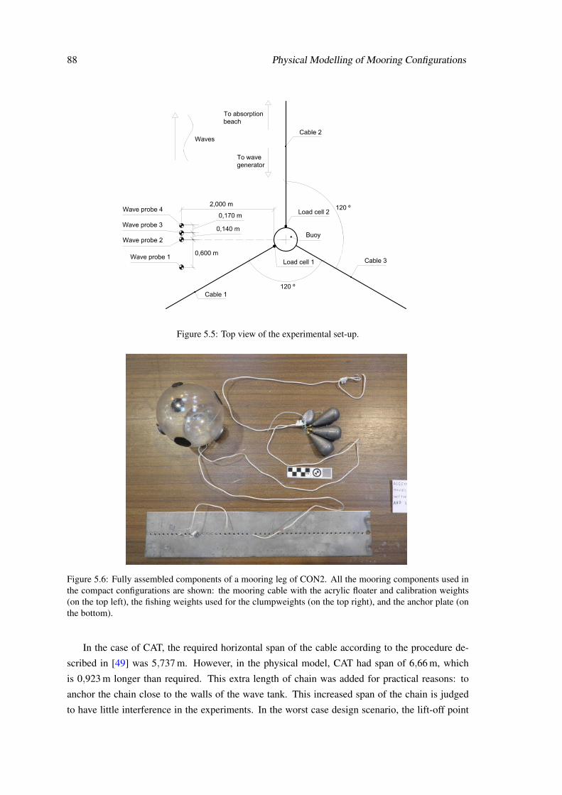
88 Physical Modelling of Mooring Configurations
Figure 5.5: Top view of the experimental set-up.
Figure 5.6: Fully assembled components of a mooring leg of CON2. All the mooring components used inthe compact configurations are shown: the mooring cable with the acrylic floater and calibration weights(on the top left), the fishing weights used for the clumpweights (on the top right), and the anchor plate (onthe bottom).
In the case of CAT, the required horizontal span of the cable according to the procedure de-
scribed in [49] was 5,737 m. However, in the physical model, CAT had span of 6,66 m, which
is 0,923 m longer than required. This extra length of chain was added for practical reasons: to
anchor the chain close to the walls of the wave tank. This increased span of the chain is judged
to have little interference in the experiments. In the worst case design scenario, the lift-off point

5.3 Experimental Set-up 89
Table 5.8: Properties of the clumpweights. Indexes 1, 2 and 3 refer to the cable where the clumpweight wasinstalled.
Mass (kg) Submerged weight (N)W1 1,115±0,001 9,968±0,001W2 1,125±0,001 10,051±0,001W3 1,113±0,001 9,959±0,001
of the chain should be at a distance of 5,737 m from the buoy, so the extra length of cable would
be resting on the floor. As both the theoretical and the actual spans of CAT are significantly larger
than the span of compact configurations (1,80 m), the extra length will not affect the ranking of
the configurations in this particular point.
The cable in the compact mooring configurations was made of polyester with a braided sheath
and a parallel strand core, Figure 5.7, and its properties are presented in Table 5.9. This type of
cable was chosen because it had negligible extension and bending stiffness in the range of tension
forces anticipated, and so elasticity would not be a significant variable in the outcome of the tests.
Figure 5.7: Sample of the synthetic cable used for the compact configurations.
Table 5.9: Properties of the synthetic cables.
EA (N) ml (kg/m) γl (N/m)(1,6±0,3)×105 (3,2±0,2)×10−3 (8,0±0,2)×10−3
The chain used to model CAT was made of zinc plated steel, Figure 5.8 and its properties are
presented in Table 5.10. It was selected, among the commercially available sizes, to be the one
with the lightest weight per unit length that could both prevent excessive displacements and have
a span that could fit in the wave tank. The acquisition of the appropriate chain to build the model
cannot be separated from the design stage, since the design depends on knowing the characteristics
of the available chains.
There is a large uncertainty in the values of the axial stiffness because the laboratory tasked
with conducting the tensile tests on the samples did not have the appropriate equipment to test

90 Physical Modelling of Mooring Configurations
Figure 5.8: Sample of the chain used in the CAT mooring.
Table 5.10: Properties of the chain.
Parameter ValueEA (1,6±0,7)×106 Nml (0,1447±0,0001) kg/mγl (1,243±0,006)N/mLink inner length (2,064±0,007)×10−2 mLink inner width (5,72±0,07)×10−3 mLink thickness (2,99±0,05)×10−3 m
cables and the procedure used was not rigorous. More details on this are provided in Annex D,
section D.9.3.
Steel blocks were used as gravity anchors for the mooring systems, Figure 5.9. Each block
was 0,50 m wide by 0,50 m deep by 0,02 m high and weighed around 333 N underwater. At the
anchor, the cables were fixed to a removable stainless steel plate to allow the quick exchange of
the mooring system and anchoring point without the need to move the anchors, Figures 5.6 and
5.9.
Figure 5.9: Top view of the anchor with its removable anchor plate (the silver grey plate in the centre).

5.3 Experimental Set-up 91
The cables were connected to the buoy using adapters bolted on the sides of the hull, Fig-
ures 5.10, which had a mass of (0,0572± 0,0018)kg. The attachment point of the cables was
located 0,220 m from the top of the buoy and 0,015 m from the surface of the hull.
Figure 5.10: Adapters used for attaching the cables and load cells to the buoy. On the left side of the adaptera pulley is installed that was meant to guide the cable to the load cell, which would be fixed to the right sideof the adapter. However, this arrangement was abandoned.
Load cells, Figure 5.11, were installed at the top-end of the left seaward cable and of the
leeward cable as shown in Figure 5.5. The right seaward cable was not instrumented because it
was assumed, due to symmetry, that the tension would be the same as in the left seaward cable.
The length of the cables where the load cells were installed was adequately shortened to account
for the length of the load cells and their accessories.
Figure 5.11: Load cell (the small steel square) used to measure the tension force in the mooring cables, withthe holding rings (used to connect the load cell to the cable and to the adapter) screwed in.
Initially, it was planned for the load cells to be screwed to one end of the adapters, remaining
fixed relative to the buoy, and for the mooring cables to go through the pulley shown in Figure 5.10,
before being attached to the load cells. This would both keep the load cells out of the water
(to avoid submergence effects) and the direction of the tension force aligned with the sensing
axes of the cells. These issues caused problems in the measurements of the tension forces in the

92 Physical Modelling of Mooring Configurations
work reported in [74]. However, preliminary tests determined that the friction in the pulleys was
unacceptably high, so it was decided to flip the adapters upside down, Figure 5.12, and install the
load cells inline, Figure 5.13. The impact of having the load-cells inline is judged to be minimal,
since their length, including accessories, was 0,046 m, their mass was only (0,0141±0,0001) kg
and the signal cables were quite thin and flexible. Due to their S-type construction, the effects of
submergence of the loads cells on the tension force readings was verified to be minimal.
(a) (b)
Figure 5.12: Installation of the adapter on the buoy. (a) general view of the adapter; (b) detailed view of theadapter, showing its orientation and position.
C
D
A
B
Figure 5.13: Inline assembly of the load cell. A - load cell adapter; B - shackle securing the load cell to theadapter; C - load cell; D - mooring cable.

5.3 Experimental Set-up 93
To measure the wave height, resistive wave probes were installed as shown in Figure 5.5. The
spacing of the probes was selected using the method of Mansard and Funke for analysis of wave
reflections, as described in the data analysis software manual [93].
The motion of the buoy was measured with an infra-red motion capture system. This sys-
tem uses infra-red cameras to emmit infra-red light and record the reflections from extremely
lightweight infra-red markers. Two of these cameras were positioned above the wave tank (one
seaward of the buoy and one leeward) and infra-red markers were placed on the buoy’s lid, Fig-
ure 5.14.
(a) (b)
Figure 5.14: Infrared system used to track the motions of the buoy: (a) markers; (b) infra-red camerasstanding on tripods on the upper catwalk.
A panorama view of the fully assembled experimental set-up for CON1 is shown in Fig-
ure 5.15. Close up views of CON2 and CAT, also when assembled in the wave tank, are shown in
Figure 5.16.

94 Physical Modelling of Mooring Configurations
Figure 5.15: Panorama view of the experimental set-up for CON1. The model is in the centre. On the leftof the photograph is the absorption beach and on the right is the wave generator. On the bottom of thephotograph are the bars that hold the wave probes.
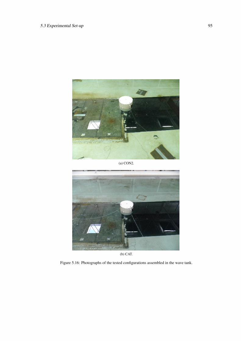
5.3 Experimental Set-up 95
(a) CON2.
(b) CAT.
Figure 5.16: Photographs of the tested configurations assembled in the wave tank.

96 Physical Modelling of Mooring Configurations
All the sensors (load cells, wave probes and motion capture) were synchronised and their data
recorded in the same computer and software; however, while the motion data was recorded directly
in engineering units, the data from the load cells and from the wave probes had to be recorded in
analogue mode (more precisely, as voltage). Post processing was required to convert the analogue
data to the proper units. A detailed uncertainty analysis for the data conversion is presented in
Annex D.
Extreme care was taken in the measurement of the properties and in the calibration of the
components of the model and of the measuring equipment. This included not only the careful
measurement of the properties and quantities themselves, but also the design and preparation of
the measuring procedures in order to have the greatest accuracy and most reliable uncertainty
quantification. The details concerning these matters are described in Annex D and were based on
the methods proposed in [54, 75, 94].
5.4 Experimental Methods
Four types of tests were conducted: i) quasi-static displacement tests, to determine the load-
excursion behaviour of the mooring systems in surge; ii) decay tests, to determine the natural
periods of the buoy-mooring system and estimates of the hydrodynamic parameters; iii) regular
wave tests, to determine the response amplitude operators and non-linear effects; and iv) irregular
wave tests, to determine the behaviour of each mooring configuration under realistic loading con-
ditions. The generated waves were long-crested, propagating in a direction parallel to the plane of
the leeward mooring cable, Figure 5.5. In this situation, the sway, roll and yaw degrees of freedom
do not have significant excitation forces and the motion of the buoy is effectively reduced to the
surge, the heave and the pitch degrees of freedom.
The quasi-static displacement tests were performed using a string to slowly pull the buoy
horizontally in direction of the x axis, Figure 5.5 (the direction of the leeward mooring cable), and
then slowly releasing the buoy back to rest position. This was done for the leeward and for the
seaward direction of the model. Particular care was taken during the tests to prevent the pulling
force on the string to rotate the buoy around the pitch axis.
In the decay tests, the buoy was displaced from its equilibrium position in a single degree of
freedom and then released. This was done for the surge, heave and pitch degrees of freedom, each
one at a time. Each test was conducted at least fifteen times in order to reduce the uncertainty in
the measurements.
In the regular wave tests, waves were generated with twenty different periods ranging from
T = 0,80s to T = 2,33s (in model scale). Around the expected resonance peaks of the system,
the wave periods were closely spaced in order to obtain a good resolution. This was done for two
target wave heights: H = 0,04m and H = 0,08m (in model scale), in order to study non-linear
effects on the behaviour of the buoy-mooring arrangement. The tests lasted 270 s in order to record

5.4 Experimental Methods 97
at least 100 waves for the longest periods and to allow for the initial transients to die out. Each
test started with the buoy in rest position, with minimal or no movement at all.
Prior to setting up the model, the regular sea-states were calibrated in order to have the average
wave height as close as possible to the target wave height. This was done by adjusting the gain of
the wave generator, a magnifying factor of the target wave height. However, the need to improve
the resolution of the response amplitude operators around the resonance peaks, required some
regular sea-states to be defined during the experiments and run without having been previously
calibrated. As a consequence, the average wave height of some of these regular sea-states is
somewhat different from the desired value. To partially compensate the lack of calibration, the
gain of these uncalibrated sea-states was estimated based on the gain of the calibrated sea-states
with the closest periods.
The irregular wave tests used the sea-states mentioned in Table 5.2. Their duration was set to
the equivalent of at least three hours in prototype scale (10800 s) as recommended in [47] and [54],
which, scaled to model values using Froude similarity (for λl = 1/100, the time scale is λt = 1/10),
resulted in a duration of 1080 s. In order to obtain sufficiently resolved spectra in post-processing,
see section 5.5, the duration of the tests was increased to 1575 s [84]. A JONSWAP spectrum
was used for the generation of the sea-states with a shape parameter γJ = 3.3, because it leads to
waves with greater steepness, as recommended in [54]. Since a pseudo-random method was used
to generate the irregular sea-states, the length of the sea-state repetition cycle (do not confuse with
the test duration) of the wave generator was set to be 1843 s [93]. This was the smallest possible
cycle length that the wave generator could create which would not be smaller than the test duration
[95].
Still in accordance with the recommendations proposed in [54], the execution of both regular
and irregular sea-states was conducted in a random order to reduce the bias effects on the experi-
ments and selected regular sea-states were repeated to assess the repeatability of the experiments.
All the tests requiring waves were run with active absorption to ensure the maximum quality
of the generated wave conditions.
To achieve a good time resolution and allow the removal of electro-magnetic interference,
the acquisition frequency of all sensors was 100 Hz. According to [93], the maximum excitation
frequency on a sea-state is expected to be around 8/TP. This excitation frequency was maximum
when TP was minimum (10 Hz for TP = 0,80s). The 4th super-harmonic of the maximum excitation
frequency will be 36 Hz, which is well below the Nyquist frequency (50 Hz) and, so, it will be
adequately captured.
As was the case for the construction of the model, proper care was taken to ensure that the
laboratory equipment was correctly used, in order to maximise the quality of the results and allow
an accurate estimate of their uncertainty. The procedures used for operation of the laboratory
equipment are described in Annex C.
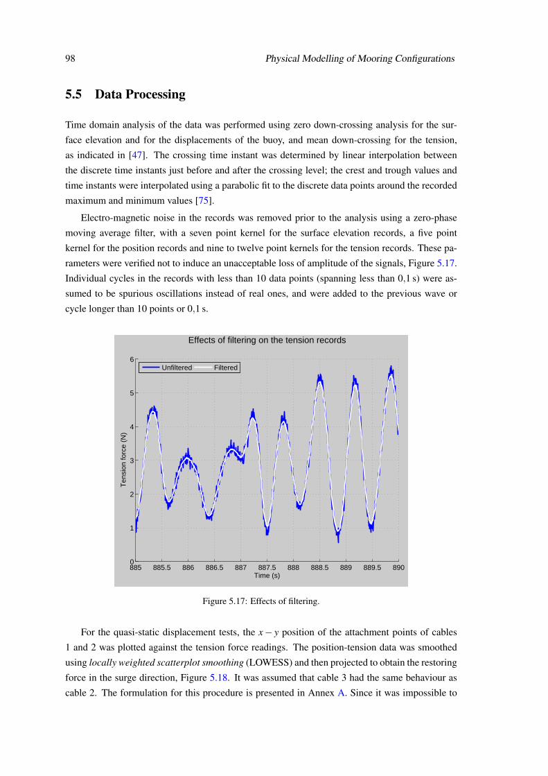
98 Physical Modelling of Mooring Configurations
5.5 Data Processing
Time domain analysis of the data was performed using zero down-crossing analysis for the sur-
face elevation and for the displacements of the buoy, and mean down-crossing for the tension,
as indicated in [47]. The crossing time instant was determined by linear interpolation between
the discrete time instants just before and after the crossing level; the crest and trough values and
time instants were interpolated using a parabolic fit to the discrete data points around the recorded
maximum and minimum values [75].
Electro-magnetic noise in the records was removed prior to the analysis using a zero-phase
moving average filter, with a seven point kernel for the surface elevation records, a five point
kernel for the position records and nine to twelve point kernels for the tension records. These pa-
rameters were verified not to induce an unacceptable loss of amplitude of the signals, Figure 5.17.
Individual cycles in the records with less than 10 data points (spanning less than 0,1 s) were as-
sumed to be spurious oscillations instead of real ones, and were added to the previous wave or
cycle longer than 10 points or 0,1 s.
885 885.5 886 886.5 887 887.5 888 888.5 889 889.5 8900
1
2
3
4
5
6
Effects of filtering on the tension records
Time (s)
Ten
sion
forc
e (N
)
Unfiltered Filtered
Figure 5.17: Effects of filtering.
For the quasi-static displacement tests, the x− y position of the attachment points of cables
1 and 2 was plotted against the tension force readings. The position-tension data was smoothed
using locally weighted scatterplot smoothing (LOWESS) and then projected to obtain the restoring
force in the surge direction, Figure 5.18. It was assumed that cable 3 had the same behaviour as
cable 2. The formulation for this procedure is presented in Annex A. Since it was impossible to

5.5 Data Processing 99
measure the inclination angle of the load cells during the tests, this angle was estimated using the
static equilibrium equations of the mooring configurations for each position of the buoy, Annex A.
−0.1 0 0.1 0.2 0.3
−10
−8
−6
−4
−2
0
2
Restoring force for CON1
Displacement (m)
For
ce (
N)
ExperimentalTheoretical
(a)
−0.1 0 0.1 0.2 0.3
−10
−8
−6
−4
−2
0
2
Restoring force for CON2
Displacement (m)
For
ce (
N)
ExperimentalTheoretical
(b)
−0.1 0 0.1 0.2 0.3
−10
−8
−6
−4
−2
0
2
Restoring force for CAT
Displacement (m)
For
ce (
N)
ExperimentalTheoretical
Figure 5.18: Restoring force as a function of the surge displacement: (a) CON1; (b) CON2; (c) CAT.
The experimental values of the restoring force in CON1 and CON2 are lower than what would
be expected (4,10 N when displaced 0,10 m, see Annex A) because of in building imperfections in
the model and because of the assumptions made in the determination of the restoring force.
The damped natural periods of the modes of motion were estimated from the data obtained in
the decay tests. For each test, the time elapsed between the first and the last crest and between
the first and the last trough was measured and divided by the number of cycles encompassed by
those time spans. The average of all the periods for each degree of freedom was taken as the best
estimate for the natural period.
It was assumed that during the decay tests, the degrees of freedom were uncoupled from each
other and that the motion was linearly damped, with constant hydrodynamic coefficients and stiff-

100 Physical Modelling of Mooring Configurations
ness. Under these assumptions, the displacement of the buoy ξ as a function of time t in each
degree of freedom can be described by [75]:
ξ (t) = ξ0 e(−ζ ·ωn·t) cos(√
1−ζ 2 ·ωn +δ
)(5.4)
where ξ0 is the initial displacement when the buoy was released, ζ is the damping factor, ωn is the
natural (undamped) angular frequency of the buoy-mooring system and δ is a phase angle. The
term ζ ·ωn in the exponential argument was determined by taking the slope of a straight line fitted
to the natural logarithm of the peaks of |ξ (t)|, Figure 5.19.
0 5 10 15 20 25 30
10−4
10−2
100
Fit of the exponential decay
Time (s)
|ξ5| (
rads
)
|ξ
5|
Fitted line
(a)
0 5 10 15 20 25 30−0.2
−0.15
−0.1
−0.05
0
0.05
0.1
0.15
0.2
Estimated decay from the initial position
Time (s)
ξ 5 (ra
ds)
ξ5
Estimated decay
(b)
Figure 5.19: Determination of the damping. (a) Example of least squares fitting a straight line to theextremes of the natural logarithm of the decaying motion of one test; (b) decay curve determined using themean exponential argument of all the tests and the initial position ξ0 of the displayed sample record.
Knowing the value of ζ ·ωn, the undamped natural frequency and the damping factor can be
estimated using the relation [75]:
ωd = ωn√
1−ζ 2 (5.5)
where ωd is the damped angular frequency of the buoy, determined directly from the damped
natural periods.
Having determined the stiffness and the undamped oscillating frequency of the buoy-mooring
system, the total mass of the system (real plus added mass), mt, is determined using the following
equation [75]:
mt = Ktω
2n (5.6)
where Kt is the stiffness of the buoy-mooring system. The added mass, ma, is obtained from
the real mass, mt (Equation 5.6), by subtracting the real mass, measured with a scale. The total

5.5 Data Processing 101
damping coefficient, bt, is determined by:
bt = 2mtζ ωn (5.7)
The total stiffness of the buoy-mooring system, Kt, as well as the individual contributions from
the buoy, Kb, and from the mooring system, Km, are frequency independent and can be determined
easily, either experimentally or analytically, as shown in subsection 5.6.1.
Both the total damping, bt, and the total mass, mt, of the model vary with frequency and
contain contributions from the buoy and from the mooring system. In order to determine the
contributions of each component of the model, first the total mass and the damping coefficient of
the buoy alone, mtb and bt
b respectively, need to be determined for the same oscillating frequency
as the coupled buoy-mooring system. Then, the contribution of the buoy is subtracted from the
total value (mt and bt) to obtain the contribution of the mooring system, mtm and bt
m, respectively.
With the available equipment it was possible to execute decay tests only at the natural frequencies
of each configuration, including the buoy floating freely. This meant that the added mass and
damping of the free buoy could only be determined for its natural frequencies, which were not the
same as when the buoy was moored. Furthermore, because there is no restoring force in surge for
an un-moored floating structure, the hydrodynamic coefficients for surge could not be determined
at all for the free buoy.
The computation of the response amplitude operators was carried out using a modification
of the method described in [85]. The regular wave records were filtered using a windowed-sinc
filter with a Blackman window [96]. This eliminated all components with periods above 3,25 s,
effectively removing any slowly varying oscillations and drift trends, Figure 5.20. Afterwards, a
Fast Fourier Transform (FFT) of the filtered record was taken and the amplitude and frequency
of the first order component extracted. These were then used as a first guess in an iterative least-
squares fitting algorithm looking for the phase, frequency and amplitude that best fit the signal
around that first guess. The quality of the fit was assessed using the coefficient of determination.
The variance spectrum of the surface elevation was determined using Welch’s method with a
Hann window and 50% overlap between sub-series [97]. The initial portion of the record with
the transients was removed and the data was filtered with a windowed-sinc filter to eliminate all
frequency components above 10 Hz. The record was then split into 31 sub-series around 97 s
long to obtain a resolution of 0,01 Hz (the exact value of the resolution varies from record to
record depending on the length of the transient portion) and estimates with a standard deviation
of 18,4 % of the mean, as recommended in [54]. In the computation of the spectral parameters,
the spectra were interpolated using zero-padding to a 65536 point FFT. The peak frequency was
determined using the centroid method proposed in [98].

102 Physical Modelling of Mooring Configurations
225 230 235 2400.12
0.13
0.14
0.15
0.16
0.17
0.18
0.19
0.2
Extraction of the linear component of surge
Time (s)
Dis
plac
emen
t (m
)
Measured motionFirst order fit
Figure 5.20: Comparison between the measured and the linear displacement component (in this case, surge).The linear component is estimated by extracting the first order component of the measured motion spectrum.
5.6 Results and Discussion
5.6.1 Quasi-static Displacement Tests
The experimentally determined plots of secant stiffness of the mooring system Km as a function of
surge displacement are presented in Figure 5.21. Just like for the restoring force, the experimental
values are lower than expected, which is both attributed to imperfections in the model and to the
assumptions made to determine the stiffness.
−0.1 0 0.1 0.2 0.320
25
30
35
40
Secant stiffness as a function of the position of the buoy
Displacement (m)
Stif
fnes
s (N
/m)
CON1CON2CAT
Figure 5.21: Secant stiffness of the configurations. The oscillations near zero displacement are due to thedivision of the force value by very small displacements.
It was not possible to experimentally determine the stiffness for heave and pitch. Instead, they
were computed using the equations of static equilibrium for each configuration (see Annex A) for

5.6 Results and Discussion 103
small displacements around the rest position (±0,01 m for heave and ±1 for pitch). The uncer-
tainty of the estimates of the stiffness for heave and pitch should be higher than for surge, since
the calculations were based on approximate assumptions for the geometry of the configurations.
5.6.2 Decay Tests
The damped natural periods of the buoy are presented in Table 5.11. As expected, the three
configurations affect the dynamics of the buoy differently, which is clear from the different values
of the natural oscillating periods.
Table 5.11: Damped natural periods of the buoy.
Mode of Motion Free CON1 CON2 CAT
Surge (s) - 8,561±0,006 9,22 ±0,08 9,14 ±0,01
Heave (s) 1,112±0,006 1,118±0,008 1,132±0,006 1,130±0,009
Pitch (s) 1,170±0,005 1,145±0,005 1,168±0,005 1,163±0,006
For surge, CON1 presents the shortest oscillating period, while CON2 and CAT present similar
oscillating periods which are slightly longer than in CON1. When compared with the free buoy,
CON1 has the least influence in the oscillating period in heave (which was already expected due
to its geometry) and CON2 has the least influence in pitch. CAT has some influence on both pitch
and heave.
To understand how the different configurations influence the dynamics of the buoy, some hy-
drodynamic parameters were estimated, Tables 5.12 to 5.14. These parameters were computed
as explained in section 5.5. There is data for only one frequency per configuration and degree
of freedom because, as mentioned in section 5.5, the decay tests could only be executed for the
natural damped frequency of each configuration.
The added mass, mab, and radiation damping coefficient, br
b, of the buoy determined using
linear potential theory [77] are also provided for comparison.
Since the added mass and damping depend on the oscillating frequency, which is different for
all configurations, a comparison of the results of the four cases might not be completely valid.
The comparison should be most accurate between CON2 and CAT, as they have similar oscillating
periods.
Because there is no restoring force in surge when the buoy is free, there is no oscillatory
motion in this situation and no parameter is estimated. The analysis in surge is justified only for
the moored situations. For heave and pitch it was possible to determine hydrodynamic parameters
for the free buoy, so it was possible to determine the total mass for the mooring system, mtm,
accounting for its real plus its added mass.
In surge, although the linear added mass of the buoy for CON1 is similar to that of CAT, and
CON1 has the smallest draft, its total mass is larger than CAT. This is probably caused by the
floaters with their large volume. The same holds for the damping coefficients.

104 Physical Modelling of Mooring Configurations
Table 5.12: Hydrodynamic parameters for surge.
Parameter Free CON1 CON2 CAT
ωd (rad/s) - 0,7339 0,6818 0,6877
ωn (rad/s) - 0,7341 0,6820 0,6879
ζ - 0,0224 0,0235 0,0242
Kt (N/m) - 28,65 28,28 23,63
Km (N/m) - 28,65 28,28 23,63
mt (kg) - 53,16 60,80 49,94
mab (kg) - 18,28 20,14 18,73
bt (kg/s) - 1,7491 1,9500 1,6658
brb (kg/s) - 0,0196 0,0182 0,0167
Table 5.13: Hydrodynamic parameters for heave.
Parameter Free CON1 CON2 CAT
ωd (rad/s) 5,650 5,620 5,551 5,560
ωn (rad/s) 5,667 5,644 5,568 5,583
ζ 0,0759 0,0924 0,0782 0,0897
Kt (N/m) 2039,5 2047,8 2059,6 2054,9
Km (N/m) - 8,3 20,0 15,4
mt (kg) 63,51 64,28 66,44 65,93
mtm (kg) - 1,48 3,49 3,00
mabe (kg) 27,67 28,44 30,60 30,09
mab (kg) 26,92 26,96 27,11 27,06
bt (kg/s) 54,67 67,04 57,90 66,00
brb (kg/s) 37,92 37,94 35,91 36,04
CON2 and CAT have similar oscillating periods, but the total mass of CON2 is around 10 kg
higher than the one of CAT, while the difference in the real masses is only 3,06 kg, Table 5.6
(relative to the hanging mass of CAT). This can support the conclusion that the floaters introduce
a significant added mass and damping (the clumpweights too, but to a lesser extent), but it might
also be caused by the higher draft of CON2 relative to CAT.
Since CON1 has a larger total mass than CAT, its shorter surge oscillating period is probably
due to the higher stiffness.
In heave, CON1 has the oscillating period closest to the free buoy because it also has the
stiffness and total mass that are closest to the values of the free buoy.
For the free buoy, the total added mass of the configuration, ma, is the same as the experi-
mentally determined added mass of the buoy alone, mabe, which is remarkably similar to value
estimated using linear potential theory, mab. It is then reasonable to assume that the estimates of

5.6 Results and Discussion 105
Table 5.14: Hydrodynamic parameters for pitch.
Parameter Free CON1 CON2 CAT
ωd (rad/s) 5,370 5,487 5,379 5,403
ωn (rad/s) 5,371 5,488 5,380 5,404
ζ 0,0140 0,0137 0,0164 0,0249
Kt (N·m) 37,76 39,41 42,43 39,44
Km (N/m) - 1,44 1,84 0,84
mt (kg·m2) 1,31 1,31 1,47 1,35
mab (kg·m2) 0,283 0,285 0,311 0,291
bt (kg·m2/s) 0,1970 0,1962 0,258 0,363
brb (kg·m2/s) 0,0493 0,0605 0,1019 0,0655
the added mass of the buoy using linear potential theory are equally accurate for the other config-
urations. In this situation, two of the four components of the total mass are known: the real and
the added masses of the buoy. The difference between the sum of these values and the total mass
of the model is the total mass of the mooring system mtm.
Using this reasoning, the mooring system of CON1 brings to the model a total mass of 1,48 kg;
CON2, with its clumpweights and floaters, brings a total mass of 3,49 kg; and the chains in CAT
bring a total mass of 3,00 kg, which is close to the value of CON2, despite the large difference in
the real masses of mooring components, Table 5.6. It seems that the chains have a large hydrody-
namic influence in heave.
When it comes to the damping coefficient, CON2 has a somewhat close value to the one of
the free buoy, while CON1 and CAT have higher damping coefficients. Since CON2 and CAT
have similar oscillating periods, but CON2 has a higher draft than CAT, it seems that the chains
cause more damping than the floaters and the clumpweights together. However, CON1, whose
major sources of damping are the floaters, has a higher damping coefficient than CAT, when it
was perhaps expected to have a smaller one. Part of this can be due to the difference in oscillating
frequencies, but it might also be that the floaters do generate high damping. The key difference
between CON1 and CON2 might be how the geometry of the mooring legs influences the motion
of the floaters. In CON1, the floaters are connected directly to the buoy, so any motion of the buoy
is transmitted straight to the floaters. On the contrary, in CON2, the displacement of the buoy
is distributed between the floaters and the clumpweights. In this configuration, the bulky floaters
have smaller motions than in CON1, therefore generation less damping, while the clumpweights
because of their a small size, do not cause an excessive increase in the damping.
In spite of having a larger damping than the free buoy, the oscillating period of CON1 is not
much longer than the free buoy because the damping factor is still small and its influence on the
oscillating frequency is of quadratic order, Equations 5.4 and 5.5.

106 Physical Modelling of Mooring Configurations
In pitch, it is CON2 that has the natural period closest to the one of the free buoy. As a coin-
cidence, the mooring system increases the stiffness and the total inertia proportionally, preventing
a large shift in the natural period.
In CON1, the only significant effect of the mooring system is increasing the stiffness and,
therefore, the natural oscillating frequency; there is almost no variation in the total mass or in the
damping coefficient when compared to the free buoy.
CAT increases both the stiffness and the total inertia, but the resulting values do not balance
as well as in the case of CON2, leading to a slightly higher natural frequency than for the free
buoy. In this case, the increased stiffness is mostly due to the larger draft of the buoy caused by
the weight of the chains, and not by the moment of the tension forces, like in CON1 and CON2,
as seen by the value of the mooring system stiffness.
Both CON2 and CAT lead to increased damping when compared with the free buoy, with CAT
having the highest damping coefficient in pitch. A possible explanation for this is that in the com-
pact configurations, the buoy can rotate with little motions of the floaters and of the clumpweights:
in CON1, the cable connected to the buoy can pivot about the connection to the floater, while in
CON2 there will be some motion of the clumpweights, but also a significant rotation of the cable
connecting them to the buoy. On the other hand, in CAT, the entire chain has to be dragged through
the water when the buoy rotates.
5.6.3 Regular Waves
The response amplitude operators (RAO) obtained with the regular wave tests are presented in
Figures 5.22 to 5.24. The displacement amplitudes in surge, ξ1, and in heave, ξ3, were non-
dimensionalised using the wave amplitude, a, and in pitch, ξ5, using the wave slope, k.
Two striking results are evident when analysing the plots: first, for each wave height and
degree of freedom, the variation of the RAO between the three configurations is unexpectedly
small; second, the wave height has a greater impact in the response than the mooring configuration.
The peak in the surge response for periods between 1,10 s and 1,20 s is not due to any resonant
motion in surge, but due to the resonant motions of heave and pitch. In all configurations, the
surge resonance period is longer than 8 s, which is much longer than the longest wave period
tested, T = 2,33s, so there is little to no surge resonant motion. For both wave heights, CON2
has the highest response amplitude for the long periods (longer than 1,10 s-1,15 s), while CON1
has the highest response for shorter periods. Looking at the damping values determined for surge
in the decay tests, Table 5.12, it would be expected that CON2, with the largest damping, had the
smallest response. However, the estimated damping is strictly valid only for the surge resonance
period. For increasingly larger periods beyond 1,30 s-1,40 s, the difference between the response
of CON2 and the responses of CON1 and of CAT becomes smaller. The excitation period is
approaching the surge resonance period and the hydrodynamic coefficients of the configurations
are probably approaching the values presented in Table 5.12, where the damping of CON2 is the
largest.

5.6 Results and Discussion 107
0.8 1 1.2 1.4 1.6 1.8 2 2.20
0.5
1
1.5
2
2.5
Surge response amplitude operator − H=0,04m
Period (s)
ξ 1 / a
CON1CON2CATCON1 Rep.CON2 Rep.CAT Rep.
1 1.1 1.20.5
1
1.5Resonance region
Period (s)
ξ 1 / a
(a)
0.8 1 1.2 1.4 1.6 1.8 2 2.20
0.5
1
1.5
2
2.5
Surge response amplitude operator − H=0,08m
Period (s)
ξ 1 / a
CON1CON2CATCON1 Rep.CON2 Rep.CAT Rep.
1 1.1 1.20.5
1
1.5Resonance region
Period (s)
ξ 1 / a
(b)
Figure 5.22: Response amplitude operator for surge. (a) response for a regular wave height H = 0,04m;(b) response for a regular wave height H = 0,08m. ξ1 - surge displacement amplitude; "Rep." denotes therepeated tests.
0.8 1 1.2 1.4 1.6 1.8 2 2.20
0.5
1
1.5
2
2.5
Heave response amplitude operator − H=0,04m
Period (s)
ξ 3 / a
CON1CON2CATCON1 Rep.CON2 Rep.CAT Rep.
1.1 1.15 1.2
1.5
2
2.5
Resonance region
Period (s)
ξ 3 / a
(a)
0.8 1 1.2 1.4 1.6 1.8 2 2.20
0.5
1
1.5
2
2.5
Heave response amplitude operator − H=0,08m
Period (s)
ξ 3 / a
CON1CON2CATCON1 Rep.CON2 Rep.CAT Rep.
1.1 1.15 1.2
1.5
2
2.5
Resonance region
Period (s)
ξ 3 / a
(b)
Figure 5.23: Response amplitude operator for heave. (a) response for a regular wave height H = 0,04m;(b) response for a regular wave height H = 0,08m. ξ3 - heave displacement amplitude; "Rep." denotes therepeated tests.
The behaviour shown in Figures 5.22a and 5.22b hints that, for devices using the surge motion
to extract energy, CON1 might be better in smaller periods while CON2 might be better for longer
ones.
In heave, CON1 has the highest response for both wave heights tested, so it will likely have
the best performance for energy extraction in this degree of freedom. The only exception occurs
at the heave resonance peak, where CON2 has a larger response. This is in line with the estimated
damping for heave presented in Table 5.13, where CON1, at the resonance frequency of heave,
has the highest damping.

108 Physical Modelling of Mooring Configurations
0.8 1 1.2 1.4 1.6 1.8 2 2.20
1
2
3
4
5
6
Pitch response amplitude operator − H=0,04m
Period (s)
ξ 5 / ka
CON1CON2CATCON1 Rep.CON2 Rep.CAT Rep.
1.1 1.15 1.22
3
4
5
Resonance region
Period (s)
ξ 5 / ka
(a)
0.8 1 1.2 1.4 1.6 1.8 2 2.20
1
2
3
4
5
6
Pitch response amplitude operator − H=0,08m
Period (s)
ξ 5 / ka
CON1CON2CATCON1 Rep.CON2 Rep.CAT Rep.
1.1 1.15 1.22
3
4
5
Resonance region
Period (s)
ξ 5 / ka
(b)
Figure 5.24: Response amplitude operator for pitch. (a) response for a regular wave height H = 0,04m;(b) response for a regular wave height H = 0,08m. ξ5 - pitch displacement amplitude "Rep." denotes therepeated tests.
For the period of 1,05 s, there is a sharp break in the response in heave, that is common to all
configurations in both wave heights. This phenomena is not due to any problem in data analysis,
but to real phenomena for this period which affected only the heave motion. For a relatively steady
wave height and period, after the initial transients of the waves and of the motion of the buoy, the
heave amplitude just slowly decreased, in an exponential way, Figure 5.25. This decaying motion
lasted for about 520 s before it stabilised (the standard duration for regular wave tests was 270 s).
An explanation for this phenomena could not be reached, but a possibility is the build up of wave
reflections inside the tank.
In pitch, CON1 has the highest response for periods up to 1,20 s to 1,30 s; for longer periods,
CON2 and CAT perform slightly better than CON1. This is similar to what happens in surge and
it is probably not a coincidence, but caused by the coupling between the two degrees of freedom.
Heave, on the contrary, is uncoupled from the other degrees of freedom [38].
There is probably a significant outlier component in the peak value of the pitch RAO of CON1
for the wave height H = 0,04 m at the period T = 1,13s, since it presents a sharp increase in the
response, in contrast with the smooth appearance of the RAO for other periods and for the other
configurations.
The response amplitude operators decrease when the wave height increases. In a purely first
order process, the RAOs should be constant when the wave height changes, so this variation is
likely due to second order and other non-linear effects. Among these, the most relevant would
be the second order drift forces (which depend on the square of the wave height), the viscous
damping, and also the non-linearity of the mooring system, whose stiffness varies with the mean
position of the buoy. All configurations seem to be equally affected by this decrease in response
amplitude, which might mean that its causes are more likely associated with the buoy than with
the mooring system.
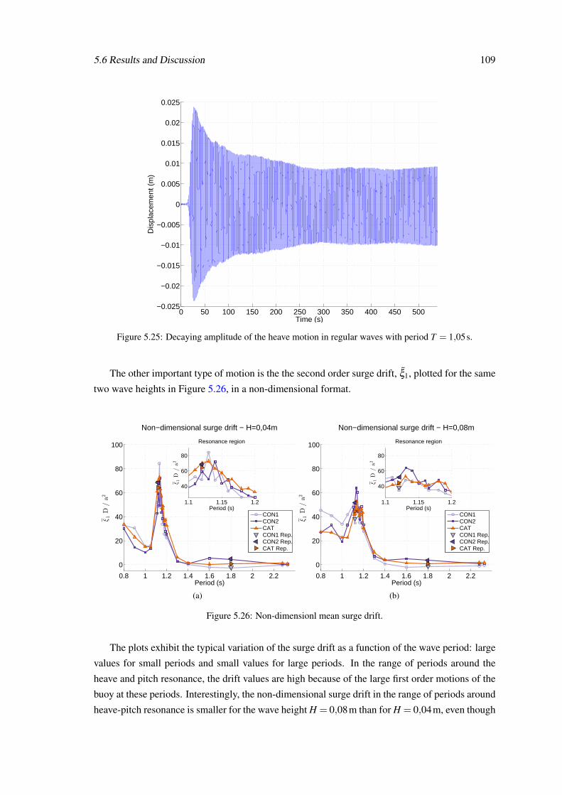
5.6 Results and Discussion 109
0 50 100 150 200 250 300 350 400 450 500−0.025
−0.02
−0.015
−0.01
−0.005
0
0.005
0.01
0.015
0.02
0.025
Decrease of the heave amplitude in regular waves with period T=1,05 s
Time (s)
Dis
plac
emen
t (m
)
Figure 5.25: Decaying amplitude of the heave motion in regular waves with period T = 1,05s.
The other important type of motion is the the second order surge drift, ξ1, plotted for the same
two wave heights in Figure 5.26, in a non-dimensional format.
0.8 1 1.2 1.4 1.6 1.8 2 2.2
0
20
40
60
80
100
Non−dimensional surge drift − H=0,04m
Period (s)
ξ1D
/a2
CON1CON2CATCON1 Rep.CON2 Rep.CAT Rep.
1.1 1.15 1.2
40
60
80
Resonance region
Period (s)
ξ1D
/a2
(a)
0.8 1 1.2 1.4 1.6 1.8 2 2.2
0
20
40
60
80
100
Non−dimensional surge drift − H=0,08m
Period (s)
ξ1D
/a2
CON1CON2CATCON1 Rep.CON2 Rep.CAT Rep.
1.1 1.15 1.2
40
60
80
Resonance region
Period (s)
ξ1D
/a2
(b)
Figure 5.26: Non-dimensionl mean surge drift.
The plots exhibit the typical variation of the surge drift as a function of the wave period: large
values for small periods and small values for large periods. In the range of periods around the
heave and pitch resonance, the drift values are high because of the large first order motions of the
buoy at these periods. Interestingly, the non-dimensional surge drift in the range of periods around
heave-pitch resonance is smaller for the wave height H = 0,08m than for H = 0,04m, even though

110 Physical Modelling of Mooring Configurations
the drift forces are four times as large in the former when compared with the later. This is probably
caused by the stiffening of the mooring system with the increasing displacement.
Although CON1 has the largest stiffness and should be better at resisting drift forces, it seems
that it allows the largest drift displacements in the smaller periods, exactly when the drift forces
have a greater importance. This was not expected.
In the range of periods of the survival sea-states, TP = 1,16s to TP = 1,42s, CON2 and CAT
have similar drifts, with CAT having slightly larger drifts than CON2. In the survivability tests
with irregular sea-states, this same result will be seen to happen as well.
Except at the heave-pitch resonance range, the plots are fairly similar between configurations
and between wave heights. The variation of the drift with the wave height and the rough shape of
the plots in general are largely due to the unsteadiness of the motion during the tests and to the
data analysis procedure. During the tests, the mean oscillating position of the buoy in surge varied
slowly, instead of being constant, as it should be in regular waves (although different than the rest
position). This could have been caused by the long period transient motion of buoy in surge, that
took a long time to die out. Only the small segments of the records where the mean position was
relatively stable could be used to estimate the drift, but they were not fully representative of the
entire records. Consequently, there is a large variability in the drift values. This variability was
amplified by the non-dimensionalisation using the square of the wave height. The waves did not
have the exact height H = 0,04m for all periods, having instead slight variations. For the smaller
waves, small variations in the wave height result in large variations of the non-dimensionalisation
constant.
Finally, there is the tension in the most loaded cable (cable 1) which is analysed from three
points of view: the average maximum tension, τmax, the mean tension, τ , and the average dynamic
tension, τdyn. The average maximum tension is the mean value of the peak tension recorded in
each oscillation in regular waves, while the average dynamic tension is defined as the mean of the
difference between the maximum and the minimum tension in each cycle.
The non-dimensional maximum tension is plotted in Figure 5.27. The results are not surpris-
ing. CON2, with the highest pre-tension, has the highest maximum tension, while CON1 and
CAT, with similar pre-tensions have similar maximum tensions.
In the region of heave-pitch resonance, the peak of the maximum tension is due to the quick
and large motions of the buoy when in resonance, which is supported by the large values of the
dynamic tension in this range, Figure 5.28.
When the wave height increases, the non-dimensional maximum tension decreases. This hap-
pens because the mean tension component of the maximum tension is almost constant, Figure 5.29,
so when the wave height increases, its non-dimensional value decreases. This effect is more no-
torious for CON2, where the non-dimensional mean tension is reduced by almost 50 % when the
wave height doubles in size, because it has the highest pre-tension (which dominates the mean
tension) of the three configurations.
Outside the resonance peak, for decreasing periods, the maximum tension seems to rise prob-
ably because of the increasing magnitude of the second order drift forces, which also increases

5.6 Results and Discussion 111
1 1.5 20
0.05
0.1
0.15
0.2
Non−dimensional maximum tensionH=0,04m
Period (s)
τmax/ρ
wgH
D2
CON1CON2CATCON1 Rep.CON2 Rep.CAT Rep.
1.1 1.15 1.2
0.040.060.080.1
0.120.14
Resonance region
Period (s)τmax/ρwgH
D2
(a)
1 1.5 20
0.05
0.1
0.15
0.2
Non−dimensional maximum tensionH=0,08m
Period (s)
τmax/ρ
wgH
D2
CON1CON2CATCON1 Rep.CON2 Rep.CAT Rep.
1.1 1.15 1.2
0.040.060.080.1
0.120.14
Resonance region
Period (s)
τmax/ρwgH
D2
(b)
Figure 5.27: Non-dimensional maximum tension.
0.8 1 1.2 1.4 1.6 1.8 2 2.20
0.01
0.02
0.03
0.04
0.05
0.06
0.07
0.08
Non−dimensional dynamic tensionH=0,04m
Period (s)
τdyn/ρ
wgH
D2
CON1CON2CATCON1 Rep.CON2 Rep.CAT Rep.
1.1 1.15 1.2
0.02
0.04
0.06Resonance region
Period (s)
τdyn/ρwgH
D2
(a)
0.8 1 1.2 1.4 1.6 1.8 2 2.20
0.01
0.02
0.03
0.04
0.05
0.06
0.07
0.08
Non−dimensional dynamic tensionH=0,08m
Period (s)
τdyn/ρ
wgH
D2
CON1CON2CATCON1 Rep.CON2 Rep.CAT Rep.
1.1 1.15 1.2
0.02
0.04
0.06Resonance region
Period (s)
τdyn/ρwgH
D2
(b)
Figure 5.28: Non-dimensional dynamic tension.
their contribution to the mean tension. For increasing periods, the maximum tension seems to rise
probably because of the interaction with the resonant motion of surge.
This analysis has a catch: the fact that CON2 has the highest maximum tension in regular
waves, does not mean that it will have the highest maximum tension in irregular waves. While
in CON2 the dynamic tension is just a fraction of the mean tension, in CON1 and in CAT both
tensions have the same magnitude. This means that both CON1 and CAT are susceptible to having
null tension in the cables (which did happen for some of the periods tested), a tell-tale sign of
imminent snap loads and high peak tensions. In fact, this is what will be seen in the results of the
irregular wave tests, where CON2 will present the best results for the tension while CON1 and
CAT will show poor performances.

112 Physical Modelling of Mooring Configurations
0.8 1 1.2 1.4 1.6 1.8 2 2.20
0.02
0.04
0.06
0.08
0.1
0.12
0.14
0.16
Non−dimensional mean tension − H=0,04m
Period (s)
τ/ρ
wgH
D2
CON1CON2CATCON1 Rep.CON2 Rep.CAT Rep.
1.1 1.15 1.20.020.040.060.080.1
0.12
Resonance region
Period (s)τ/ρwgH
D2
(a)
0.8 1 1.2 1.4 1.6 1.8 2 2.20
0.02
0.04
0.06
0.08
0.1
0.12
0.14
0.16
Non−dimensional mean tension − H=0,08m
Period (s)
τ/ρ
wgH
D2
CON1CON2CATCON1 Rep.CON2 Rep.CAT Rep.
1.1 1.15 1.20.020.040.060.080.1
0.12
Resonance region
Period (s)
τ/ρwgH
D2
(b)
Figure 5.29: Non-dimensional mean tension.
The similarity between the dynamic tension plots for 0,04 m and 0,08 m waves indicates that,
in the range of periods tested, it should vary linearly with the wave height, just like the first order
wave loads and motions that induce the dynamic tension.
In general, CON1 has the highest dynamic tension for both wave heights, with the exception of
the resonance periods for H = 0,08m. CON2 has practically no variation in the dynamic tension
when the wave height changes, while CAT has a 25 % increase for H = 0,08m when compared
with H = 0,04m.
Just like for the drift, the tension plots do not have a smooth appearance, which is both due
to the unsteadiness of the tension, and to the tension cycles in some of the periods tested having
several peaks. Most of these peaks were above the mean tension value and so they were detected
in the zero-crossing analysis. Averaging all the values of all of the peaks in each record resulted
in average peak values lower than what they would be if only the single largest peak in each cycle
was detected. An example of this is shown in Figure 5.30.
Another consequence of the multi-peak shape of the tension cycle is the fatigue damage to
the cables. Although this effect was not a research priority in these experiments, some important
conclusions can be made. The existence of several peaks per cycle will increase the fatigue damage
to the cables, especially when the tension is high.
CON2 presents the most complex cycles, which can have more than three peaks each. The
mooring legs in this configuration (with a floater and a clumpweight) together with the buoy, act
as three degree-of-freedom oscillator, that has three natural oscillating frequencies, and might have
other complex non-linear interactions.
CON1, with a floater, acts as a two degree of freedom oscillator and has two natural oscillating
frequencies. The tension cycles are not as complex as for CON2, but it still has multi-peak cycles.
CAT acts simply as a spring and has only one natural oscillating frequency. Nevertheless,
it also shows several peaks per cycle in some periods, probably because of the non-linearity of
mooring systems. No configuration is immune to this effect.
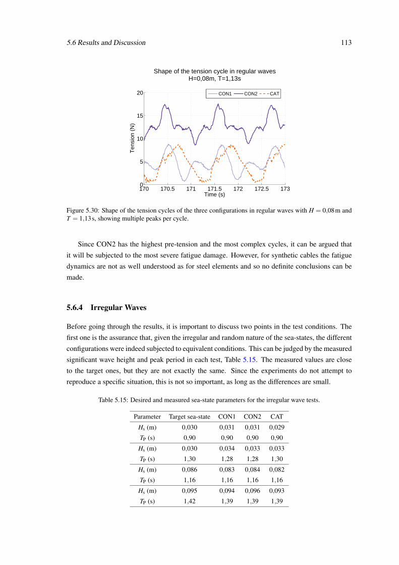
5.6 Results and Discussion 113
170 170.5 171 171.5 172 172.5 1730
5
10
15
20
Shape of the tension cycle in regular wavesH=0,08m, T=1,13s
Time (s)
Ten
sion
(N
)
CON1 CON2 CAT
Figure 5.30: Shape of the tension cycles of the three configurations in regular waves with H = 0,08m andT = 1,13s, showing multiple peaks per cycle.
Since CON2 has the highest pre-tension and the most complex cycles, it can be argued that
it will be subjected to the most severe fatigue damage. However, for synthetic cables the fatigue
dynamics are not as well understood as for steel elements and so no definite conclusions can be
made.
5.6.4 Irregular Waves
Before going through the results, it is important to discuss two points in the test conditions. The
first one is the assurance that, given the irregular and random nature of the sea-states, the different
configurations were indeed subjected to equivalent conditions. This can be judged by the measured
significant wave height and peak period in each test, Table 5.15. The measured values are close
to the target ones, but they are not exactly the same. Since the experiments do not attempt to
reproduce a specific situation, this is not so important, as long as the differences are small.
Table 5.15: Desired and measured sea-state parameters for the irregular wave tests.
Parameter Target sea-state CON1 CON2 CAT
Hs (m) 0,030 0,031 0,031 0,029
TP (s) 0,90 0,90 0,90 0,90
Hs (m) 0,030 0,034 0,033 0,033
TP (s) 1,30 1,28 1,28 1,30
Hs (m) 0,086 0,083 0,084 0,082
TP (s) 1,16 1,16 1,16 1,16
Hs (m) 0,095 0,094 0,096 0,093
TP (s) 1,42 1,39 1,39 1,39

114 Physical Modelling of Mooring Configurations
What matters is that the generated test conditions for each target sea-state are the same for
the three configurations. As the maximum difference between test conditions is 6,9 % for the
significant wave height (sea-state OP1) and 1,5 % for the period (sea-state OP2), it can be assumed
that the test conditions are much the same for all the configurations. Furthermore, each target sea-
state had only one realisation of the random wave phases, which meant that even the generated
time series were the same for the three configurations.
The realisation of the wave phases brings up the second point: the variability of the results
due to the randomness of the waves. In order to establish with some confidence the results of the
irregular wave tests, each target sea-state would have to be run with, at least, ten different wave
phase realisations. Due to lack of time, it was only possible to have one realisation, which is not
enough to cover the possible variability of the results. When the results of the three configurations
do not show significant differences, the conclusions might be hindered by this bias.
Now, for the evaluation of the performance of the different configurations, the major factor
to consider is the power extraction. Since there was no power take-off installed, this is estimated
using the mean squared velocity of the buoy in each degree of freedom, Table 5.16. For a linearly
damped power take-off, the mean squared velocity can be assumed to be proportional to the aver-
age power that would be extracted by the device. This assumption can be up for debate, but it will
at least provide an estimate.
Table 5.16: Displacement in operational sea-states. ξ1 - surge; ξ3 - heave; ξ5 - pitch; p.p - peak-to-peak am-plitude. Overbar denotes mean value.
OP1 OP2
Parameter CON1 CON2 CAT CON1 CON2 CAT
ξ 1 (·10−3 m) 6,1 5,3 5,6 4,8 4,3 4,6
ξ 1p.p (·10−3 m) 19,8 18,1 16,1 19,6 20,0 17,5
ξ 21 (m2/s2) 0,064 0,059 0,060 0,088 0,085 0,073
maxξ1 (·10−3 m) 46,2 43,8 43,3 47,4 43,6 40,0
ξ 3p.p (·10−3 m) 9,1 8,5 8,5 25,3 25,1 24,5
ξ 23 (m2/s2) 0,048 0,039 0,040 0,271 0,263 0,250
maxξ3 (·10−3 m) 13,5 13,5 13,0 35,6 34,3 33,0
ξ 5p.p() 3,8 3,4 3,2 9,1 8,5 7,8
ξ 25(rad2/s2) 2,348 1,827 1,649 11,043 9,4708 7,775
maxξ5() 5,4 4,9 4,5 10,7 10,2 9,1
CON1 allows the highest power extraction in both sea-states in all degrees of freedom. This
is in accordance with the general analysis of the response amplitude operators, sub-section 5.6.3,
where CON1 had an overall better performance than CON2 and than CAT. CON2 appears as the
second best configuration, since its performance is lower than CAT only for surge and heave and
only in sea-state OP1; CAT is, then, the configuration with the worst overall performance in terms
of power extraction.

5.6 Results and Discussion 115
Judging from the surge response amplitude operator, Figure 5.22a, it would be expected that
CON2 had a better performance than CON1 for the sea-state OP2 (TP = 1,30s), which does not
happen. However, the differences between the response amplitude operators of CON1 and CON2
and between the mean squared velocities of the three configurations for TP = 1,30s in surge are
small and might be due to experimental variability and randomness.
For pitch, in OP2 (TP = 1,30s), CAT should have a slightly better performance than CON1,
Figure 5.24a, or, at least, similar, Figure 5.24b. Instead, CAT has the worst performance and
CON1 has the best one, with a difference of almost 42 % in power extracted. The fact that CAT
has a higher estimated total damping, Table 5.14, can be a possible explanation for the lower
performance in irregular seas, when compared with regular waves. Once again, randomness might
have had an impact on the results.
The remaining motion parameters (ξ , ξ p.p and maxξ ) follow the same trend as the mean
squared velocity (which is consistent), but with even smaller differences between configurations.
In operational sea-states, peak tensions are, usually, not an important factor, since they tend to
be much smaller than in survival conditions. However, they are presented in Table 5.17 because of
an interesting situation: CON1 is already showing both large dynamic tensions (equal to or greater
than the mean tension) and, up to the uncertainty in readings, null tensions. In contrast, CON2 and
CAT have low dynamic tensions and are able to keep both cables under tension. The potential for
this situation was already highlighted in sub-section 5.6.3.
Table 5.17: Tension in operational sea-states. τ - tension; p.p - peak-to-peak amplitude. Overbar de-notes mean value. Indexes 1 and 2 refer to the cable where the tension was measured.
OP1 OP2
Parameter CON1 CON2 CAT CON1 CON2 CAT
Hs (m) 0,031 0,031 0,029 0,034 0,033 0,033
TP (s) 0,90 0,90 0,90 1,28 1,28 1,30
τ1 (±0,2N) 2,9 10,8 3,1 2,9 10,7 3,1
maxτ1 (±0,2N) 5,8 11,9 3,6 5,1 12,1 3,9
minτ1 (±0,2N) 0,2 9,6 2,7 0,7 9,2 2,4
τdyn1 (±0,3N) 2,9 1,1 0,5 2,2 1,5 0,8
τ2 (±0,2N) 3,0 11,1 3,0 3,0 11,1 3,0
maxτ2 (±0,2N) 6,6 12,3 3,6 5,9 12,6 3,8
minτ2 (±0,2N) 0,1 9,9 2,5 0,3 9,3 2,0
τdyn2 (±0,3N) 3,6 1,2 0,6 2,9 1,6 0,8
For the survival sea-states, the focus is on the extreme motions and tensions, Tables 5.18 and
5.19.
To ensure the integrity of power lines (or similar components connected to the wave energy
converter) and to avoid possible crashes between devices, the most relevant criterion is the maxi-
mum surge displacement.

116 Physical Modelling of Mooring Configurations
Table 5.18: Displacements in survival sea-states. ξ1 - surge; ξ3 - heave; ξ5 - pitch; p.p - peak-to-peak am-plitude. Overbar denotes mean value.
SURV1 SURV2
Parameter CON1 CON2 CAT CON1 CON2 CAT
ξ 1 (·10−3 m) 62,5 63,2 63,6 31,9 39,0 39,6
ξ 1p.p (·10−3 m) 131,2 135,2 119,5 81,7 92,8 90,0
maxξ1 (·10−3 m) 311,6 318,6 278,7 186,8 222,7 210,8
maxξ1p.p (·10−3 m) 428,5 442,0 348,9 247,5 286,8 255,3
ξ 3p.p (·10−3 m) 71,6 69,6 66,6 74,8 70,7 71,6
maxξ3 (·10−3 m) 87,2 83,4 77,6 108,9 98,5 100,9
maxξ3p.p (·10−3 m) 171,7 164,3 154,8 198,4 183,1 183,0
ξ 5p.p() 21,8 19,1 18,0 17,6 14,8 15,5
maxξ5() 25,7 22,2 20,7 21,3 17,4 18,8
maxξ5p.p() 44,6 38,7 37,1 40,2 34,0 35,1
In section 5.2, in the design of the mooring system, the maximum surge displacement allowed
for the buoy was set to be 0,200 m, which is far exceed by all configurations. The reason for this,
already mentioned in section 5.2, is the fact that the mooring legs were initially designed to be
opposite to each other, but were later installed in a triangular arrangement, reducing the overall
stiffness in surge.
The largest surge displacement occurs, in both sea-states, in CON2; CAT has the best results
in the sea-state SURV1, while in sea-state SURV2 it is CON1. The inferior performance of CON2
might be due to it having more components subjected to drift forces (floaters and clumpweights)
than CON1 or CAT. As before the differences between the values of the three configurations are
too small to exclude randomness of the sea-states as the cause for these results.
The extreme surge displacement might be interpreted under a different light. Figure 5.31
shows all the peak values of the surge displacement in the survival sea-states, ranked by their mag-
nitude. For CON1, in the sea-state SURV1, the last two values are repeated. This almost certainly
means that this configuration reached a state where the mooring leg is fully taut. Although this
does not imply the failure of the mooring system, when the cable is fully taut the tensions can
increase sharply, so this condition should be avoided. This situation, which did not happen for any
other configuration, could mean that CON1 has a limited displacement only because it reached a
deformation limit.
Figure 5.31 reveals another interesting effect. While for sea-state SURV2 (TP = 1,42s) the
peak values rise steadily with the rank for all configurations, in sea-state SURV1 (TP = 1,16s)
there is a sudden increase in the peak magnitudes when the rank reaches 100 to 125. Also, there are
fewer, but significantly larger peaks for sea-state SURV1 when compared with sea-state SURV2.
The examination of the response amplitude operator of surge for waves with height H = 0,08m,
Figure 5.22b, shows that the surge response for the period T = 1,16s should be slightly higher
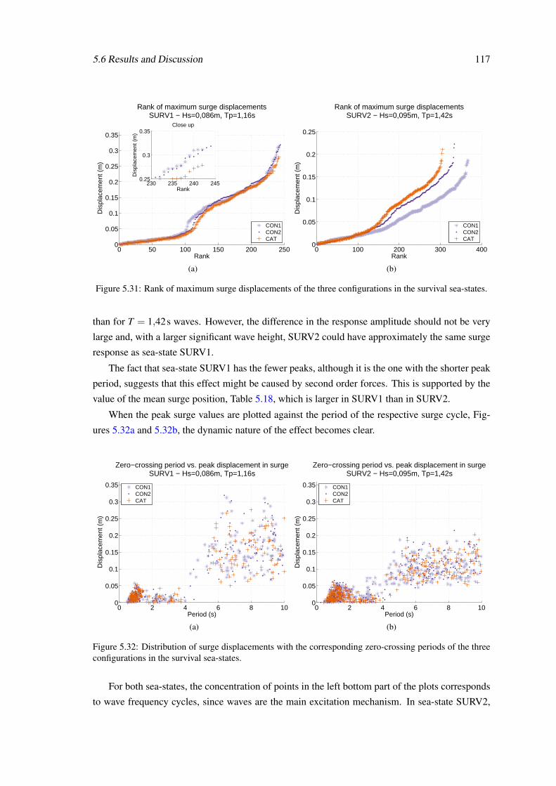
5.6 Results and Discussion 117
0 50 100 150 200 2500
0.05
0.1
0.15
0.2
0.25
0.3
0.35
Rank of maximum surge displacementsSURV1 − Hs=0,086m, Tp=1,16s
Rank
Dis
plac
emen
t (m
)
CON1CON2CAT
230 235 240 2450.25
0.3
0.35Close up
Rank
Dis
plac
emen
t (m
)
(a)
0 100 200 300 4000
0.05
0.1
0.15
0.2
0.25
Rank of maximum surge displacementsSURV2 − Hs=0,095m, Tp=1,42s
Rank
Dis
plac
emen
t (m
)
CON1CON2CAT
(b)
Figure 5.31: Rank of maximum surge displacements of the three configurations in the survival sea-states.
than for T = 1,42s waves. However, the difference in the response amplitude should not be very
large and, with a larger significant wave height, SURV2 could have approximately the same surge
response as sea-state SURV1.
The fact that sea-state SURV1 has the fewer peaks, although it is the one with the shorter peak
period, suggests that this effect might be caused by second order forces. This is supported by the
value of the mean surge position, Table 5.18, which is larger in SURV1 than in SURV2.
When the peak surge values are plotted against the period of the respective surge cycle, Fig-
ures 5.32a and 5.32b, the dynamic nature of the effect becomes clear.
0 2 4 6 8 100
0.05
0.1
0.15
0.2
0.25
0.3
0.35
Zero−crossing period vs. peak displacement in surgeSURV1 − Hs=0,086m, Tp=1,16s
Period (s)
Dis
plac
emen
t (m
)
CON1CON2CAT
(a)
0 2 4 6 8 100
0.05
0.1
0.15
0.2
0.25
0.3
0.35
Zero−crossing period vs. peak displacement in surgeSURV2 − Hs=0,095m, Tp=1,42s
Period (s)
Dis
plac
emen
t (m
)
CON1CON2CAT
(b)
Figure 5.32: Distribution of surge displacements with the corresponding zero-crossing periods of the threeconfigurations in the survival sea-states.
For both sea-states, the concentration of points in the left bottom part of the plots corresponds
to wave frequency cycles, since waves are the main excitation mechanism. In sea-state SURV2,

118 Physical Modelling of Mooring Configurations
the remaining points are more or less evenly distributed in the plot. However, for the sea-state
SURV1, there is a second cluster of points, although not very pronounced, in the 8 s-10 s interval.
This period interval encompasses the surge resonance periods of the mooring configurations. This
suggests that the jump in the magnitude of the peaks in sea-state SURV1 is caused by excitation
in the surge resonance period, which is likely to come from second order forces. It is interesting
to note that this second order excitation affects the three configurations similarly.
Extreme displacements and extreme displacement amplitudes (not necessarily the same) might
cause damage to several components of a wave energy converter, especially to electrical cables and
to the power take-off system. Most designs try to avoid this by incorporating safety mechanisms
in the device itself, because it might be challenging to conceive a mooring system that can both
allow large displacements in operational conditions and prevent large displacements in survival
conditions. Nevertheless it is important to see how the different configurations behave in this
aspect.
CON2, which has the largest surge displacements, has also the largest surge amplitudes for
both sea-states. In heave and pitch, CON1 has both the largest displacement and the largest dis-
placement amplitude. This should not be a surprise, since CON1 is the best for extracting energy
because it allows greater motions of the buoy.
CAT has the smallest displacement and displacement amplitudes for sea-state SURV1 in all
degrees of freedom. This is in agreement with the response amplitude operators for T = 1,16s,
Figures 5.23b and 5.24b, where CAT presents the smallest value. In sea-state SURV2, CAT has
the second smallest displacements and displacement amplitudes, but they are very close to the
actual smallest values. In extreme displacements, CAT seems to be the configuration with the best
performance.
For the purpose of safe station-keeping, the critical factor is the extreme tension in the cables:
maximum, minimum and dynamic, Table 5.19. In irregular waves, as defined in [47], the dynamic
tension is the difference between the absolute maximum tension and the mean tension.
The time series of the tension in cable 1 for the three configurations in the survival sea-states
are plotted in Figure 5.33. Some aspects the behaviour of the configuration can be quickly grasped
just by looking at the this figure: CON1 has a low mean tension, with moderate and closely spaced
peak tensions; CON2 has a high mean tension, but small and relatively spaced peak tensions; the
catenary has low mean tension, with sharp and high peak tensions.
The extreme tensions occur, for all the configurations and for both cables, in sea-state SURV1.
This is the sea-state that generates the most intense response in surge, the mode of motion that is
most influenced by the mooring system.
CON2 has the highest maximum tension values. Even though the tension behaviour is far from
linear, this should be anticipated, as CON2 has also the highest pre-tension.
Within the uncertainty of the measurements, CON2 and CAT have the same maximum tension,
around 17 N, which is the absolute maximum tension recorded. This is somewhat surprising,
since the pre-tension in CAT is significantly lower than in CON2. The consequence of this is that

5.6 Results and Discussion 119
Table 5.19: Tension in survival sea-states.p.p - peak-to-peak amplitude. Overbar denotes mean value. In-dexes 1 and 2 refer to the cable where the tension was measured.
SURV1 SURV2
TP = 1,16s TP = 1,42s
Parameter CON1 CON2 CAT CON1 CON2 CAT
τ1 (±0,2N) 3,6 11,2 3,8 3,2 11,0 3,4
maxτ1 (±0,2N) 11,0 17,3 17,5 9,6 14,8 11,2
minτ1 (±0,2N) 0,0 6,5 0,2 0,0 7,8 0,3
τdyn1 (±0,3N) 7,4 6,2 13,7 6,4 3,9 7,8
τ2 (±0,2N) 2,3 10,5 2,4 2,6 10,7 2,6
maxτ2 (±0,2N) 8,9 15,1 8,6 8,0 13,6 6,6
minτ2 (±0,2N) 0,0 5,7 0,5 0,0 7,1 0,7
τdyn2 (±0,3N) 6,5 4,6 6,2 5,4 2,8 4,0
although CAT has a lower pre-tension, it would have to be designed to withstand the same forces
as CON2.
In CON1 and in CAT the minimum tension in both cables and in both sea-states is practically
0,0 N. CON2, on the other hand, never presented tensions below 9,2 N. Keeping the cables under
tension is important to avoid snap loads and local compression in the cables and CON2 is the only
one that meets this requirement.
The dynamic tensions in CON1 and in CAT are larger than in CON2. In fact, in CON1 and in
CAT the dynamic tension is almost as large as the maximum tension, while in CON2 the dynamic
tension is around half of the maximum tension. This is the direct result of CON1 and CAT allowing
the tension to go to 0 N, which results in snap loads. This can be seen more clearly in Figure 5.34,
where peak and dynamic tensions are plotted, for each configuration, by the rank of their peak
tensions: the higher tensions are always associated with high dynamic tensions.
CON2 is probably the best configuration when it comes to tension in the cables because it has
the smallest dynamic loading and its mooring components have to resist peak loads that are not
much higher than the mean load.
Overall, CON1 stands out as a good choice to maximize power production, but it has a poor
performance in tension in the cables. CON2, being a hybrid between a compact configuration
such as CON1 and a heavy configuration such as CAT, gathers the strong points from both. It
seems to be a good compromise solution, with smaller values of extracted power than CON1 (yet
higher than CAT), but with an excellent performance of the dynamic behaviour of the mooring
cables. CAT has the best performance in minimizing the extreme displacements and displacement
amplitudes, which is important mostly for surge, where active mechanisms to protect wave energy
converters might not be feasible. However, it has the worst performance in power extraction and
generates very high dynamic tensions. Additionally, it takes a lot of space in the seabed.

120 Physical Modelling of Mooring Configurations
0 500 1000 15000
5
10
15
20
Time series of the tension in cable 1 of CON1SURV1 − Hs=0,086m, Tp=1,16s
Time (s)
Ten
sion
(N
)
(a)
0 500 1000 15000
5
10
15
20
Time series of the tension in cable 1 of CON2SURV1 − Hs=0,086m, Tp=1,16s
Time (s)
Ten
sion
(N
)
(b)
0 500 1000 15000
5
10
15
20
Time series of the tension in cable 1 of CATSURV1 − Hs=0,086m, Tp=1,16s
Time (s)
Ten
sion
(N
)
(c)
0 500 1000 15000
5
10
15
20
Time series of the tension in cable 1 of CON1SURV2 − Hs=0,095 m, Tp=1,42s
Time (s)
Ten
sion
(N
)
(d)
0 500 1000 15000
5
10
15
20
Time series of the tension in cable 1 of CON2SURV2 − Hs=0,095 m, Tp=1,42s
Time (s)
Ten
sion
(N
)
(e)
0 500 1000 15000
5
10
15
20
Time series of the tension in cable 1 of CATSURV2 − Hs=0,095 m, Tp=1,42s
Time (s)
Ten
sion
(N
)
(f)
Figure 5.33: Time series of the tension in cable 1 in the survival sea-states. (a) - (c) SURV1; (d) - (f)SURV2.

5.7 Additional Remarks 121
0 500 1000 1500 20000
5
10
15
20
Rank of tensions in cable 1SURV1 − Hs=0,086m, Tp=1,16s
Rank
Ten
sion
(N
)
Peak tension CON1Peak tension CON2Peak tension CATDyn. tension CON1Dyn. tension CON2Dyn. tension CAT
(a)
0 500 1000 1500 20000
5
10
15
20
Rank of tensions in cable 1SURV2 − Hs=0,095m, Tp=1,42s
Rank
Ten
sion
(N
)
Peak tension CON1Peak tension CON2Peak tension CATDyn. tension CON1Dyn. tension CON2Dyn. tension CAT
(b)
Figure 5.34: Rank of peak tensions and associated dynamic tensions for the three configurations in survivalsea-states. (a) SURV1; (b) SURV2
5.7 Additional Remarks
The choice of the best configuration depends also on other factors, such as weather variability,
restrictions related to the impact of certain types of anchors or mooring configurations on the
seabed, etc. In sheltered regions or in regions where the difference between operational and sur-
vival conditions is not very large, mooring systems like CON1 might perform better than in the
tests presented here, when it comes to keeping the cables under tension. The type of soil might
hinder the use of drag embedment anchors or anchors resisting vertical loads, which would not
allow some of the configurations to be used at all.
The position of the attachment point of the mooring cables (fairlead) has an influence in the
dynamic behaviour of wave energy converters. Attaching all the mooring cables to a single point
on the device would decouple the pitch motion from the motions of the mooring cables, which
could improve power extraction in pitch or, at least, make it less dependent on the mooring system.
The irregular tests presented here were performed using long crested waves acting on a single
device without power take-off. When the devices are set-up in dense arrays and subjected to
short-crested waves, both the displacements of the devices and the tensions in the cables will
be magnified [86]. The use of a power take-off in operational conditions will also increase the
tensions in the cables and the surge drift, when compared to the results presented [50].
Despite the differences between configurations, some of the results, such as the response am-
plitude operators, show only small variations between configurations. On the one hand, this might
mean that the configurations have little effect on the dynamics of the buoy. On the other hand, this
might mean that the results are dominated by the large size and mass of the buoy compared to the
size of the other components of the model, due to the use of a distorted scale.

122 Physical Modelling of Mooring Configurations
As mentioned in section 5.1, tests were performed to assess sensitivity of the results of the
compact configurations to variations of their properties. These results could not be presented here,
but they will be the subject of a future publication.
Finally, each sea-state in the irregular wave tests had only one random phase realisation, which
was used for the three configurations (but different realisations between sea-states). Being a ran-
dom event, several realisations should have been done for each sea-state ([47] requires at least 10)
in order to remove the variability of the results. This was not done due to the limited time available
for testing. As a consequence, and because the results do not have a very large variation between
the three configurations, there will be some uncertainty in the conclusions.
5.8 Conclusions
Three mooring configurations for wave energy converters were tested in physical models and the
results presented. The configurations were: (i) a compact mooring arrangement composed of a
synthetic cable with an intermediate floater (CON1); (ii) a compact mooring configuration com-
posed of a synthetic cable with a floater and a clumpweight, creating a zig-zag pattern (CON2);
and (iii) a catenary (CAT).
The parameters analysed included those commonly used in the design of mooring systems,
such as maximum surge displacement or maximum loads in the cables, but also parameters rel-
evant to wave energy converters, such as the mean squared velocity in each mode of motion (to
estimate power extraction) or peak-to-peak amplitudes (to estimate extreme loads in the power
take-off).
CON1 provided the best results for power extraction and had the least interference in the heave
motion (where its natural period is almost the same as for the buoy floating freely). This happens
because the vertical motion of the wave energy converter is decoupled from the motions of the
mooring cables. However, this configuration was not so good at maintaining the tension in cables
and had high dynamic tensions in extreme conditions.
CON2 did not have as good a performance in power extraction as CON1, but it proved to be
superior in handling the tension in the cables. It was able to keep the cable under tension at all
times, while simultaneously minimising the dynamic tension. It had also the smallest impact in
the natural pitch period. In general, it seems to be a good compromise between CON1 and CAT,
combining the strong points of both with its own strong points, in a globally optimised solution.
CAT had a good performance in extreme sea-states, where it limited the maximum displace-
ments and the maximum displacement amplitudes. The downside of this is that it also had the
worst performance in power extraction. Like CON1, it was not able to keep the cable under ten-
sion at all times and, additionally, it had the largest dynamic tension, leading to the highest maxi-
mum tension. It had also, by far, the largest footprint of the three configurations, which results in
added costs and environmental impact. Still, even though it has not been especially designed for
wave energy converters, CAT might have an acceptable performance, depending on the working
principle of the device and on the sea-states in which it should operate.

5.8 Conclusions 123
In spite of the ranking of each configuration for each parameter, the differences between the
configurations are not large in any situation.

124 Physical Modelling of Mooring Configurations

Chapter 6
Conclusions
Three major outcomes were obtained with this thesis: (i) a numerical model for the simulation
of mooring cables; (ii) a technique to track the motions of mooring cables in small scale models;
and (iii) the physical model study of mooring configurations for offshore wave energy converters.
These results try to answer the needs, outlined in the Introduction, of new tools for the study and
development of mooring systems for wave energy converters and of an improved understanding
of their dynamic behaviour.
The numerical model developed used the spectral/hp-element discontinuous Galerkin method
to solve the partial differential equation of perfectly flexible cables. It was able to reproduce both
analytical and experimental results with remarkable quality. The model did not perform so well
in the simulation of a physical model of a moored buoy. However, this cannot be fully attributed
to the numerical model. On the contrary, it is probably the result of having used linear potential
theory to simulate the dynamics of the buoy (which does not account for important second order
effects) and of the considerable uncertainty in some of the data measured in the physical model
experiments.
Due to its higher order discontinuous formulation, the numerical model demonstrated expo-
nential convergence to the solution and evidenced the ability to capture shocks, in the form of peak
tensions. These goals were targeted from the beginning. Additionally, the use of a discontinuous
formulation resulted in the mass matrix of the numerical model being block diagonal, which can
be inverted more efficiently than the sparse matrices of continuous formulations. All of these char-
acteristics result in the numerical model being capable of providing high accuracy solutions using
coarse discretisations. Theoretically, it is also possible to obtain faster computational times using
this numerical model than lower order or continuous ones. However, this very much depends on
the time-marching scheme used and on the programming language in which the numerical model
is coded. Higher order methods require smaller time-steps than lower order ones, which might
counteract the gain of using coarser discretisations.
The experimental technique to track mooring cables was able to capture the full length of a
mooring cable in a wave tank when the buoy it secured was excited by waves. As it captured the
full length of the cable, it also captured singularities that would remain undetected by techniques
125

126 Conclusions
tracking a discrete set of points along the cable. An example of such singularity was the break in
the slope of the cable at the point where it touches the floor of the wave tank, while it was moving
back and forth.
The algorithm developed to process the videos proved to be robust enough to work even when
visibility conditions were far from ideal. However, in spite of its robustness, some care was still
required in the preparation of the experimental set-up. More specifically, when viewed from the
camera, the experimental set-up cannot have any detail in the vicinity of the cable with a dimension
similar to the thickness of the cable. It was also necessary to ensure enough contrast between the
cable and the background of the image.
The range of application of the technique is wide, from concept design to fundamental re-
search on mooring cable dynamics. By outputting the geometry of cables as a function of time,
this technique provides data that was previously hard to obtain. This information can be used to
validate and calibrate numerical models, to determine the regions where the cable is mostly likely
to be damaged by dragging or rubbing against the seabed, etc.
By post-processing the videos it is possible to determine the velocity and the acceleration of
desired points along the cable. When this is combined with measurements of water velocity in the
vicinity of the cable, it becomes possible to study the hydrodynamic drag and inertia effects of
mooring cables.
Using the common measurements of water surface elevation and tension in the cable, the data
provided by the technique allows deeper studies of phenomena such as snap loads, shock waves
caused by the cable hitting the seabed, correlation of the tension in the cable with its geometry and
velocity, with the wave phase, etc.
Although applied only in a two dimensional experiment, there is no inherent limitation pre-
venting the use of the technique in three-dimensional cases.
The physical model experiments of mooring systems analysed three different configurations:
CON1, using taut synthetic cables with a floater near the surface; CON2, using taut synthetic
cables with a floater and a clumpweight creating a zig-zag shape; and CAT, a chain catenary.
The general conclusion of the experiments is that no single mooring configuration can be
selected as the absolute best to secure a floating wave energy converter. All the configurations have
advantages that cannot be matched by the others, and their relevance depends on many parameters,
of which the type of wave energy converter is just one.
CON1, using taut cables and floaters, allowed motion dependent devices to have the best per-
formance in power extraction because it allowed larger motions, but this might not be so important
for motion independent devices. Being compact it used little material, had a reduced weight and
allowed a dense arrangement of devices in arrays, all of which are important in reducing the cost
of deployment. This configuration was also the one causing the smaller difference between the dy-
namic behaviour of the free buoy and of the moored buoy, so it is the one which allows developers
to design a wave energy converter with the least concern about the impact of the mooring system.
However, it was not so good at coping with high dynamic tensions and extreme displacements.

Conclusions 127
CON2, using taut cables, floaters and clumpweights did not perform as well as CON1 in
terms of energy extraction, but the difference was small. However, it was the best configuration at
keeping the dynamic tensions low, and it was the only one that was able to prevent the mooring
cables from getting slack. Like CON1, it has several advantages because it is compact, but more
material is required for clumpweights, which also make it heavier and, therefore, more expensive
than CON1.
In comparison with CON1 and CON2, CAT had the worst performance when it came to allow-
ing energy to be extracted by motion dependent devices, but it was the best at preventing extreme
displacements. Like CON1 it was susceptible to high dynamic tensions and, some times, allowed
the cables to become slack. An apparent disadvantage when compared to CON1 and CON2 is that
it occupied a considerable space on the seabed and does not allow devices to be deployed in dense
arrays. However, since it uses cheaper anchoring technology than CON1 and CON2, and it is an
already established technology, it can well be a good choice for motion independent devices.

128 Conclusions

Chapter 7
Suggested Future Developments
7.1 Numerical Model for Mooring Cables
One of the most important subjects to be analysed in the numerical model is the existence of
high frequency ripples. These are especially apparent when the tension is low and when the
cable impacts the ground. It is not known whether these are physical phenomena captured by
the numerical model or numerical artefacts that should be dealt with. For this it will likely be
necessary the development of improved models describing the interaction between the cable and
the ground, to eliminate this as a possible cause.
It is also suggested that the results of the numerical model be compared with more experi-
mental data. This data should come from simple experiments, with high accuracy measurements
and broad parametric variations. There should be a reduced number of variables influencing the
behaviour of the cables in the experiments, and complex physical models, such as the case of the
moored buoy used in this work, should be avoided. Possible set-ups include the use of a motor
to drive one end of the cable in a periodic motion. Only after the conduction of these tests, and
the nuances of the numerical model are thoroughly investigated and well understood, should its
results be compared with complex physical models: first with a cable subjected only to waves,
then subjected to both waves and forced motions of the top end, and finally subjected to waves
while mooring a simple buoy.
Also required is the formal demonstration of the properties of the numerical model, namely
its convergence and shock capturing ability, as well as a more thorough study of the non-standard
stabilisation parameter λ2.
For improved performance it is suggested the application of implicit time-stepping schemes
and coding the model in languages such as Fortran or C++, although this is more a technical issue.
129

130 Suggested Future Developments
7.2 Tracking Technique for Mooring Cables in Physical Models
Reducing the error associated with the technique is the foremost important development to achieve
engineering and scientific quality. This will require the use of equipment with enhanced optical
quality than the one used in this work. After this, the next step, if needed, is the development
or the application of improved procedures to linearise the camera and calibrate the experimental
set-up. The complexity of the work required for this task depends on the optics used and on their
quality.
Also necessary, even with high-quality optical equipment, is development calibration proce-
dures, that can determine how the error, the distortion and the calibration factors are distributed
across the image, and estimate local corrections and conversion factors.
The algorithm should be expanded so that it becomes able to track single and multiple segment
cables, with floaters and clumpweights, in three dimensions. This requires more the application of
already existing knowledge than carrying out research, but it is vital for the technique to be truly
powerful.
The possibility of tracking the trajectory of specified points on the cable after acquiring the
videos, as well as of determining the velocity and acceleration of all the sections of the cable,
should also be included in the algorithm, instead of being a post-processing step. Once this
achieved, the technique can be used to its full potential by combining it with measurements water
velocity around the cable.
Sub-pixel interpolation, although not critical, will also be an interesting development.
Some simplification of the methods should also be considered, aimed at reducing the work
required by the operator using the technique. This should include the automatic detection of the
cable in the videos and the elimination of the need to linearise the camera for each experiment.
7.3 Experimental Work
There are two important improvements that are strongly suggested. One is the determination
of the hydrodynamic properties of the buoy and of the mooring cables, separately, for different
oscillating frequencies, with and without waves. This will allow a better use of the experimental
results, since it will be possible to estimate with much greater accuracy the impact of the mooring
configurations. The other is the test of the configurations with different phase realisations for the
same sea-state conditions.
It is also important that the mooring configurations be tested with different directions of the
incoming waves and with different positions of the attachments of the cables to the hull. Variations
on the pre-tension have been tested, but not yet fully analysed. Other parametric variations can be
imagined to be tested with the same physical model. And, of course, it can even be suggested the
definition of new configurations for analysis.
Considering a wider variation of the experimental set-up, it is necessary to test the configura-
tions in properly scaled models, instead of distorted ones. This task can be considerably difficult

7.3 Experimental Work 131
because it requires dynamic scaling of the stiffness of the cables, of the floater and of the clump-
weights.
The configurations should ultimately be tested in arrays, which will require large wave tanks,
in order to examine the interaction between devices. A power take-off can be included in future
experiments. This should be done with some care, since it causes changes in the dynamics of the
buoy and reduces the scope of the conclusions to specific types of power take-off system.

132 Suggested Future Developments

Appendix A
Mooring Design
A.1 Design Loads and Displacements
Water depth: 0,900 m
xmax (20% of the water depth) = 0,180m≈ 0,200m
Maximum significant wave height of the design sea-states, Hs−max = 0,0950m
Maximum expected wave height Hmax = 2Hs−max = 0,190m≈ 0,200m
The first order (wave frequency) displacements of the free buoy, xw, in regular waves were
estimated using linear potential theory and are presented in Table A.1.
Table A.1: First order horizonal displacements of the free buoy estimated using linear potential theory.
T (s) xw(m)
0,9 0,0581,1 0,0801,3 0,0501,8 0,099
xw = 0,099m≈ 0,100m
xs = xmax− xw = 0,100m
Fxs =23
ρwg(
H∗s2
)2
r (A.1)
where H∗s is an increased value of the maximum significant wave height, to account for the effect
of the slowly varying forces. The parameters used in equation A.1 and the magnitude of the second
order drift forces are presented in Table A.2.
133

134 Mooring Design
Table A.2: Parameters for the estimation of the second order wave forces.
Parameter Valueρw (kg/m3) 1000g (m/s2) 9,81H∗s (m) 0,100r (m) 0,25725Fxs (N) 4,0875
The mooring systems must be able to provide a horizontal restoring force of at least 4,1 N
when the buoy is displaced horizontally from rest position by 0,100 m, which is equivalent to a
horizontal secant stiffness of 41 N/m.
A.2 Equations of Static Equilibrium of the Mooring Configurations
O
B
A
x
z
α
βFF
τ2τ2
τ1
τ1
Figure A.1: Free body diagram for CON1. FF - buoyancy force of the floaters.
OA2= x2
A + z2A (A.2)
AB2= (xB− xA)
2 +(zB− zA)2 (A.3)
τ1 sin(α) = FF + τ2 sin(β ) (A.4)
τ1 cos(α) = τ2 cos(β ) (A.5)

A.2 Equations of Static Equilibrium of the Mooring Configurations 135
O x
z
α
βθ
τ1
τ1
FF
FS
τ2 τ2
τ3
τ3
AB
C
Figure A.2: Free body diagram for CON2. FF - buoyancy force of the floaters; FS - submerged weight ofthe clumpweights.
OA2= x2
A + z2A (A.6)
AB2= (xB− xA)
2 +(zB− zA)2 (A.7)
BC2= (xC− xB)
2 +(zC− zB)2 (A.8)
τ1 sin(α) = FF +T2 sin(β ) (A.9)
τ1 cos(α) = τ2 cos(β ) (A.10)
τ2 cos(β ) = τ3 cos(θ) (A.11)
FF = τ1 sin(α)+ τ2 sin(β ) (A.12)
FS = τ2 sin(β )+ τ3 sin(θ) (A.13)

136 Mooring Design
α
y
x
τ1h
τ1h
τ2h
τ3hFrx
A
B
C
D
Figure A.3: Horizontal components of the restoring force. Frx - horizontal restoring force in the x direction;τih - horizontal component of the tension force in cable i.
tan(α) = (xB− xA)/(yB− yA) (A.14)
τ1hx = τ1hx sin(α) (A.15)
Frx = τ2hx− (τ1hx + τ3hx) (A.16)
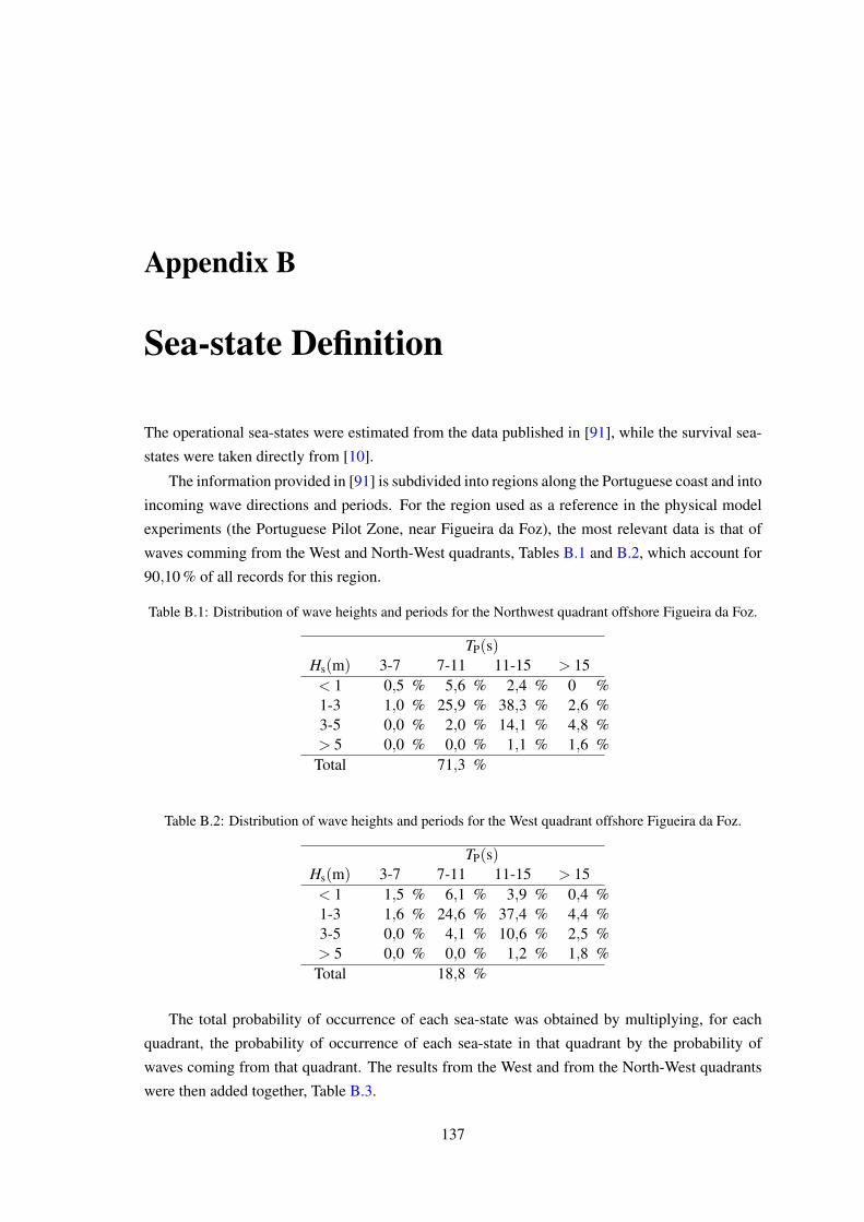
Appendix B
Sea-state Definition
The operational sea-states were estimated from the data published in [91], while the survival sea-
states were taken directly from [10].
The information provided in [91] is subdivided into regions along the Portuguese coast and into
incoming wave directions and periods. For the region used as a reference in the physical model
experiments (the Portuguese Pilot Zone, near Figueira da Foz), the most relevant data is that of
waves comming from the West and North-West quadrants, Tables B.1 and B.2, which account for
90,10 % of all records for this region.
Table B.1: Distribution of wave heights and periods for the Northwest quadrant offshore Figueira da Foz.
TP(s)Hs(m) 3-7 7-11 11-15 > 15< 1 0,5 % 5,6 % 2,4 % 0 %1-3 1,0 % 25,9 % 38,3 % 2,6 %3-5 0,0 % 2,0 % 14,1 % 4,8 %> 5 0,0 % 0,0 % 1,1 % 1,6 %
Total 71,3 %
Table B.2: Distribution of wave heights and periods for the West quadrant offshore Figueira da Foz.
TP(s)Hs(m) 3-7 7-11 11-15 > 15< 1 1,5 % 6,1 % 3,9 % 0,4 %1-3 1,6 % 24,6 % 37,4 % 4,4 %3-5 0,0 % 4,1 % 10,6 % 2,5 %> 5 0,0 % 0,0 % 1,2 % 1,8 %
Total 18,8 %
The total probability of occurrence of each sea-state was obtained by multiplying, for each
quadrant, the probability of occurrence of each sea-state in that quadrant by the probability of
waves coming from that quadrant. The results from the West and from the North-West quadrants
were then added together, Table B.3.
137

138 Sea-state Definition
Table B.3: Wave height and period distribution for the combined West and Northwest quadrants offshoreFigueira da Foz.
TP(s)Hs(m) 3-7 7-11 11-15 > 15< 1 0,6 % 5,1 % 2,4 % 1,9 %1-3 1,0 % 23,1 % 34,3 % 4,3 %3-5 0,0 % 2,2 % 12,0 % 1,6 %> 5 0,0 % 0,0 % 1,0 % 1,5 %
The estimates of available energy were determined by multiplying the probability of occur-
rence of each sea-state by the respective average power density, P, (using the average significant
wave height and peak period of the range), Table B.4, through the equation:
P =Hm0
2Teρwg2
64π(B.1)
where Hm0 is the estimate of the significant wave height from the wave spectrum, ρw is the water
density, g is the magnitude of the acceleration of gravity and Te = 1,2/1,4TP is the energy period.
Table B.4: Estimated yearly available energy distribution offshore Figueira da Foz (W·year/m).
TP(s)Hs(m) 5 9 13 > 15
0,5 3 49 33 302 85 3496 7509 10724 0 1330 10536 16265 0 0 1380 2333
Two sea-states were selected for the periods with the most available energy (TP = 9s and
TP = 13s) by taking, for each period, the mean of the two wave heights with the most available
energy (Hs = 2m and Hs = 4m), Table B.5.
Table B.5: Selected irregular sea-states.
Hs (m) TP (s)3,0 9,03,0 13,0

Appendix C
Usage of Equipment
This annex describes the procedures for calibration and operation of the equipment used in the
experimental work.
C.1 Wave Tank
The wave tank of the Faculty of Engineering of the University of Porto is equipped with a multi-
paddle piston wave maker, with active absorption. All tests, including the calibration of the wave
tank, were run using active absorption.
The calibration of the tank was executed in order to assure that, at the position where the model
was to be installed, the wave heights and periods of the sea-states had, as much as possible, the
desired values.
To calibrate the tank, all the planned sea-states were run without the model in the wave tank,
while wave probes recorded the surface elevation at the position where the model was to be in-
stalled. After a sea-state was run, the average wave height (for the regular tests) or the significant
wave height (for the irregular tests) was determined. If the measured value of the wave height was
off from the desired value, a gain would be applied to the initial value of the target wave height
until the desired wave weight was reached.
After each experiment was executed in the wave tank, including the decay tests, the water in
the wave tank was allowed to settle for at least 20 min for any waves to die out before the next test
was started.
C.2 Load Cells and Wave Probes
The data from the load cells and from the wave probes were recorded as voltage in the same
computer used to track the motion of the buoy. To achieve this, the analogue voltage signal form
the probes and from the load cells was passed through an analogue-to-digital (A\D) converter
type PCI-DAS1602/16 manufactured by Measurement Computing. As per recommendation of the
139
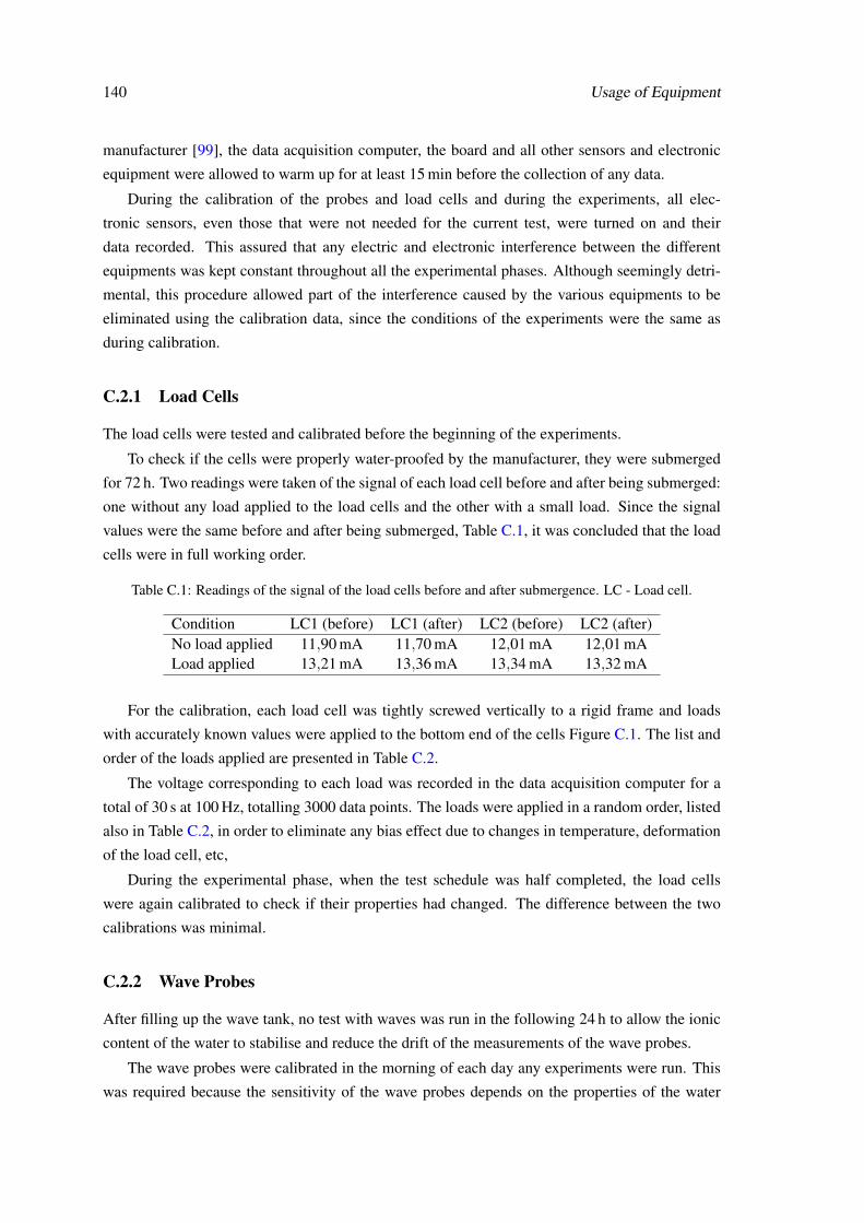
140 Usage of Equipment
manufacturer [99], the data acquisition computer, the board and all other sensors and electronic
equipment were allowed to warm up for at least 15 min before the collection of any data.
During the calibration of the probes and load cells and during the experiments, all elec-
tronic sensors, even those that were not needed for the current test, were turned on and their
data recorded. This assured that any electric and electronic interference between the different
equipments was kept constant throughout all the experimental phases. Although seemingly detri-
mental, this procedure allowed part of the interference caused by the various equipments to be
eliminated using the calibration data, since the conditions of the experiments were the same as
during calibration.
C.2.1 Load Cells
The load cells were tested and calibrated before the beginning of the experiments.
To check if the cells were properly water-proofed by the manufacturer, they were submerged
for 72 h. Two readings were taken of the signal of each load cell before and after being submerged:
one without any load applied to the load cells and the other with a small load. Since the signal
values were the same before and after being submerged, Table C.1, it was concluded that the load
cells were in full working order.
Table C.1: Readings of the signal of the load cells before and after submergence. LC - Load cell.
Condition LC1 (before) LC1 (after) LC2 (before) LC2 (after)No load applied 11,90 mA 11,70 mA 12,01 mA 12,01 mALoad applied 13,21 mA 13,36 mA 13,34 mA 13,32 mA
For the calibration, each load cell was tightly screwed vertically to a rigid frame and loads
with accurately known values were applied to the bottom end of the cells Figure C.1. The list and
order of the loads applied are presented in Table C.2.
The voltage corresponding to each load was recorded in the data acquisition computer for a
total of 30 s at 100 Hz, totalling 3000 data points. The loads were applied in a random order, listed
also in Table C.2, in order to eliminate any bias effect due to changes in temperature, deformation
of the load cell, etc,
During the experimental phase, when the test schedule was half completed, the load cells
were again calibrated to check if their properties had changed. The difference between the two
calibrations was minimal.
C.2.2 Wave Probes
After filling up the wave tank, no test with waves was run in the following 24 h to allow the ionic
content of the water to stabilise and reduce the drift of the measurements of the wave probes.
The wave probes were calibrated in the morning of each day any experiments were run. This
was required because the sensitivity of the wave probes depends on the properties of the water

C.2 Load Cells and Wave Probes 141
Figure C.1: Set-up for calibration of the load cells. The load cell is the small square rectangle on the top ofthe image, from which a load is hanging on a hook.
Table C.2: Loads applied in the calibration of the load cells.
Order of application Load (±0,001N)1 1,0502 97,7663 2,0214 19,6105 68,5236 5,0037 0,5598 9,8309 48,981
10 0,26511 0,16712 87,99613 39,08314 0,00015 0,06916 58,742
which varied from day to day (for example, the mineral content) and some times even during the
same day.
Only three points were used for calibrating the wave probes: 0,000 m, 0,040 m and −0,040 m
relative to a standard position. These three points were judged to be enough as they correspond to
a height difference of 0,080 m, which includes the range of all regular waves and all but the largest
third of the irregular waves in the survival sea-states. As the wave probes are highly linear, the use
of more points was not required.

142 Usage of Equipment
The prongs of the wave probes were all parallel to the wave front and care was taken to ensure
that the wave probes were aligned with each other and with the wave direction.
After assembly in the wave tank, the mast securing each probe was aligned vertically using a
spirit level to minimise any reading errors due to tilts.
As recommended by the manufacturer [93], the distance between the wave probes was mea-
sured at the water surface.
C.3 Motion Capture
The motion capture system was assembled, calibrated and operated according the the specifica-
tions of the manufacturer [100]. It was only calibrated sporadically when the need arose, which
would happen when either the cameras or the infra-red markers on the buoy were accidentally
disturbed. After each test the data recorded by the motion capture system was checked in order
to ensured that the measurement residue was below 0,002 m. Unfortunately, this value cannot be
translated directly into an uncertainty in the position of the buoy, because the manufacturer of the
motion tracking system did not provide the necessary information for these calculations.
C.4 Centre of Gravity
The centre of gravity was determined indirectly, by balancing the buoy on a horizontal rotation
axis, Cr, and applying an external load, F , to the hull, as illustrated in Figure C.2. Without any
load applied, the buoy would (theoretically) remain in a vertical position. By applying the external
load to the top of the hull, in a direction 90 to the horizontal rotation axis, a moment is created
which causes the buoy to rotate by an angle α .
Cg
Cr
F
dcc
hCr
ycgr
α
W
Figure C.2: Schematics of the procedure for the determination of the centre of gravity. Cg - centre of gravity;Cr - centre of rotation.

C.4 Centre of Gravity 143
The moment of the external load is counter-balanced by the moment due to the weight W of
the buoy. Knowing α it is possible to determine the vertical distance dcc between the rotation axis
and the centre of gravity, Cg, by the following equation:
dcc =FW
(hCr +
rtan(α)
)(C.1)
For the experimental determination of the centre of gravity, the rotation axis was created by
two steel wedges screwed to the hull of the buoy at diametrically opposed positions, Figure C.3.
The buoy with the wedges was placed on flat horizontal supports, that allowed the buoy to rotate
around the tip of the wedges, Figure C.4.
Figure C.3: Steel wedge screwed to the hull of the buoy used in the determination of the centre of gravity.
The rotation angle α caused by the application of the external load was measured with a digital
inclinometer placed on the lid of the buoy, as close as possible to its longitudinal axis, Figure C.5.
Measurements were made with different loads, applied in random order, first on the front of the
buoy and then on the back. The wedges were installed in two different directions 90 to one
another (N-S and E-W, Figure C.6), providing a total of four sets of readings.
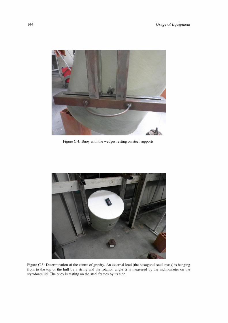
144 Usage of Equipment
Figure C.4: Buoy with the wedges resting on steel supports.
Figure C.5: Determination of the centre of gravity. An external load (the hexagonal steel mass) is hangingfrom to the top of the hull by a string and the rotation angle α is measured by the inclinometer on thestyrofoam lid. The buoy is resting on the steel frames by its side.

C.4 Centre of Gravity 145
N
S
EW
Figure C.6: Nomenclature of the directions of the horizontal axes on the buoy.

146 Usage of Equipment
C.5 Moment of Inertia
The inertia of the buoy around the horizontal axis through the centre of gravity was determined
indirectly, by hanging the buoy by cables attached to the hull and swinging it like a pendulum,
Figure C.7.
dRC
Cg
R
Figure C.7: Schematics of the set-up used to determine the inertia of buoy. dRC - distance from the pivotpoint R to the centre of gravity Cg.
Knowing the period of the oscillation, the inertia can be determined using the following equa-
tion:
Icg =
(T2π
)WdRC−mbd2
RC (C.2)
where Icg is the mass moment of inertia through the centre of gravity, T is the oscillation period,
W is the weight of the buoy, mb is the mass and dRC is the distance between the centre of gravity
and the pivot point of the cables, R.
The cables holding the buoy were attached at diametrically opposed sides, at the same height
in order to prevent torsional motions while swinging. To measure the period, a smartphone was
placed on the lid of the buoy with an application recording the acceleration as a function of time.
C.6 Calibration of the Floaters
The buoyancy of the floaters was calibrated by placing the floaters in a water filled basin and
attaching a clumpweight to each one. The clumpweights had been previously calibrated, so their
submerged weight was accurately known and was at most 0,05 N off from the desired 10,00 N
value. Afterwards, small weights (stainless steel washers and small pieces of lead) were added

C.6 Calibration of the Floaters 147
to each floater until they would barely be able to float. At this point, the buoyancy of the floaters
would be almost exactly the same as the submerged weight of the clumpweights, but with unknown
uncertainty.
By trial and error, small pieces of rubber were placed on top of each floater (only one at each
try) until it was found the smallest piece that would cause each floater to sink. The uncertainty
in the buoyancy of the floaters was assumed to be the submerged weight of the largest piece of
rubber used, which was 0,06 N.

148 Usage of Equipment

Appendix D
Uncertainty Analysis
D.1 General Method
The estimation of the standard uncertainty uX of a property X follows the division of uncertainty
sources into systematic and random. The systematic uncertainty is denoted by bX , while the
random uncertainty, when applicable, is the standard deviation sX of the values of X [94]. The
standard uncertainty is obtained as follows:
uX =√
sX2 +b2
X (D.1)
The expanded uncertainty of UXk%, with a confidence of k% is obtained from uX by:
UXk% = tk%uX (D.2)
where tk% is the coefficient from the Student t-distribution for the k% probability, with the adequate
degrees of freedom. The expanded uncertainty for all values presented in this work is the UX95%.
When the number of measurements is equal to, or greater then 10, sometimes the coefficient tk%
was simplified to the value 2 [94].
When the mean value X of a sample of X is used to estimate the mean of the parent population,
µX , the standard deviation of the mean, sX , is obtained from the standard deviation of the sample
of X , sX , from:
sX =sX√
N(D.3)
where N is the number of samples used to estimate X .
In situations where several measurements are required to estimate the value of a variable, the
best estimate is taken to be the mean of the measurements, X . When the measurement is obtained
as a single reading from a measuring equipment which, independently of how many repetitions are
149

150 Uncertainty Analysis
made, will always be the same, the best estimate is the value X itself. In this case, the uncertainty
of the measuring equipment is assumed to be the UX95%. An example of this could be the weight
measured by a scale.
When the final result must be obtained from equations combining different variables, the un-
certainty in the final result is propagated from the input variables using the Taylor Series Method.
For a property f that is a function of several variables
f = f (X1,X2, ...,Xi, ...,Xn) (D.4)
the uncertainty is estimated in the following way:
u f =
√∑
(∂ f∂Xi
)2 (bi
X + siX
)2 (D.5)
where siX and bi
X are, respectively, the random and the systematic uncertainty in quantity X due to
variable i.
D.2 Calibrated Masses
The properties of the masses used to apply the loads in the determination of the centre of gravity
and in the calibration of the load cells are listed in Table D.1.
Table D.1: Properties of the masses used in the determination of the centre of gravity and in the calibrationof the load cells.
Name Mass (×10−3 kg) Um95%(×10−3 kg) Weight (×10−3 N) Uw95%(×10−3 N)1 1,008 0,001 9,88848 0,009812 2,030 0,001 19,91430 0,009815 5,011 0,001 49,15791 0,0098110 10,006 0,001 98,15886 0,0098120 20,038 0,001 196,57278 0,0098150 49,447 0,001 485,07507 0,00981100 99,716 0,001 978,21396 0,00981200 198,55 0,01 1947,7755 0,0981500 502,78 0,01 4932,2718 0,09811000 995,36 0,01 9764,4816 0,09812000 1992,07 0,01 19542,2067 0,09812000’ 1985,3 0,01 19475,7930 0,09815000 4985,86 0,01 48911,2866 0,0981Hook 7,1 0,1 69,651 0,981

D.3 Height of the Buoy 151
D.3 Height of the Buoy
The average height of the buoy was determined from four measurements around its perimeter,
Table D.2. The uncertainty calculations are presented in Table D.3.
Table D.2: Measurements of the height of the buoy.
Measurement Value (m)1 0,40002 0,40003 0,40154 0,4005
Table D.3: Estimation of the uncertainty in the height of the buoy.
Parameter ValueHb (m) 0,4005bHb (m) 0,0005sHb (m) 0,000707106781sHb
(m) 0,00040824829uHb (m) 0,000645497224t95% 3,182UHb95% (m) 0,002053972168

152 Uncertainty Analysis
D.4 Diameter of the Buoy
The average diameter of the buoy was determined from two measurements at its top, in two or-
thogonal directions, Table D.4. The uncertainty calculations are presented in Table D.5.
Table D.4: Measurements of the diameter of the buoy.
Measurement Value (m)1 0,51452 0,5145
Table D.5: Estimation of the uncertainty in the diameter of the buoy.
Parameter ValueDb (m) 0,5145bDb (m) 0,0005sDb (m) 0,0000sDb
(m) 0,0000uDb (m) 0,0005t95% 4,3030UDb95% (m) 0,0022
D.5 Determination of the Centre of Gravity
The position of the centre of gravity was estimated using the method described in section C.4,
equation C.1:
dcc =FW
(hCr +
rtan(α)
)(D.6)
where the variables dcc, F , W , hCr, r and α are defined in Figure C.2. The uncertainty in the posi-
tion of the centre of gravity was estimated using the relations derived below, from equation D.6:
udcci =
√∑
(∂dcc
∂X j
)2 (bX j
)2 (D.7)
where udcci is the uncertainty in the measurement i of distance dcc and X j are the variables in equa-
tion D.6. There is no random uncertainty in the calculation of udcci because, for each measurement
with a certain applied load, the values of the variables were always the same, no matter how
many times the measurement is repeated. The uncertainties udcci are condensed into the systematic
uncertainty of the estimation of dcc using in the following way:
bdcc =√
∑(udcci)2/N (D.8)

D.5 Determination of the Centre of Gravity 153
where N is the number of measurements. The uncertainty in the position of the centre of gravity
relative to the bottom of the buoy, including random uncertainty, is then calculated as demonstrated
below:
udcc =
√∑
(b2
dcc+ s2
dcc
)(D.9)
ycg = Hb− (dcc +hCr) (D.10)
uycg =√
u2Hb
+u2dcc
+u2hCr
(D.11)
The value of the variables used in the determination of the position of the centre of gravity and
of its uncertainty are listed in Table D.6. The results obtained for the distance dcc in each mea-
surement are listed in Table D.7. The results of the intermediate calculations of the uncertainty are
presented in Tables D.8 and D.9 and the final results of the uncertainty are presented in Table D.10.
Table D.6: Value of the parameters required for the estimation of the uncertainty in the position of the centreof gravity.
Parameter Value uX
Mass, mb (kg) 35,50 0,05W (N) 348,255 0,4905r (m) 0,25725 0,002α (rad) - 0,0017453293F (N) - 0,0009907614hCr (m) N/A 5,15×10⁻⁴
Hb (m) 0,400 6,22×10⁻⁴

154 Uncertainty Analysis
Table D.7: Measurements of the distance dcc.
Axis hCr (m) Loads applied Total mass (kg) F (N) α() dcc
N-S Forward 0,2015 2000 1992,07 19,5422067 8,0 0,1140209726N-S Forward 0,2015 5000 4985,86 48,9112866 21,6 0,1195538067N-S Forward 0,2015 1000 995,36 9,7644816 4,2 0,1038701182N-S Forward 0,2015 2000+2000’ 3977,37 39,0179997 16,8 0,1180386063N-S Forward 0,2015 5000+1000 5981,22 58,6757682 26,8 0,1197538707N-S Forward 0,2015 2000+1000 2987,43 29,3066883 11,9 0,1196855962N-S Backward 0,2015 2000 1992,07 19,5422067 6,6 0,1360694235N-S Backward 0,2015 5000 4985,86 48,9112866 20,2 0,1264982941N-S Backward 0,2015 1000 995,36 9,7644816 2,8 0,1531272630N-S Backward 0,2015 2000+2000’ 3977,37 39,0179997 15,3 0,1279309997N-S Backward 0,2015 5000+1000 5981,22 58,6757682 25,4 0,1252294336N-S Backward 0,2015 2000+1000 2987,43 29,3066883 10,8 0,1304414374E-W Forward 0,2020 2000 1992,07 19,5422067 7,3 0,1240077832E-W Forward 0,2020 5000 4985,86 48,9112866 20,9 0,1229500657E-W Forward 0,2020 1000 995,36 9,7644816 3,3 0,1307503918E-W Forward 0,2020 2000+2000’ 3977,37 39,0179997 16,0 0,1231177927E-W Forward 0,2020 5000+1000 5981,22 58,6757682 26,1 0,1224654935E-W Forward 0,2020 2000+1000 2987,43 29,3066883 11,5 0,1233828910E-W Backward 0,2020 2000 1992,07 19,5422067 7,5 0,1209695868E-W Backward 0,2020 5000 4985,86 48,9112866 21,5 0,1200563026E-W Backward 0,2020 1000 995,36 9,7644816 3,8 0,1142514771E-W Backward 0,2020 2000+2000’ 3977,37 39,0179997 16,6 0,1192850200E-W Backward 0,2020 5000+1000 5981,22 58,6757682 26,6 0,1205454033E-W Backward 0,2020 2000+1000 2987,43 29,3066883 12,1 0,1179583824

D.5
Determ
inationofthe
Centre
ofGravity
155
Table D.8: Partial derivatives of equation D.6 with respect to its variables, for each measurement presented in Table D.7.
Measurement ∂dcc/∂F×10−3 (m/N) ∂dcc/∂hCr×10−2 ∂dcc/∂ r×10−1 ∂dcc/∂α×10−1 (m/) ∂dcc/∂W ×10−4 (m/N)1 5,834600684 5,611464789 3,992764666 7,452826611 −3,2740656292 2,444298954 14,044676056 3,547280249 2,666106791 −3,4329386993 10,637545589 2,803830986 3,818091302 13,447201869 −2,9825879944 3,025234691 11,203859155 3,710897185 3,450100755 −3,3894303395 2,040942528 16,848507042 3,335437473 2,132060882 −3,4386834556 4,083900403 8,415295775 3,993344030 5,091313223 −3,4367229817 6,962848443 5,611464789 4,849847306 10,927247343 −3,9071778868 2,586280242 14,044676056 3,817231171 3,030250166 −3,6323468199 15,682067852 2,803830986 5,732849118 30,226103943 −4,396986777
10 3,278768791 11,203859155 4,095441147 4,139357633 −3,67348637311 2,134261509 16,848507042 3,548287342 2,355773690 −3,59591200612 4,450910184 8,415295775 4,411452534 6,165555414 −3,74557256713 6,345638702 5,611464789 4,380433545 8,940924333 −3,56083281414 2,513736078 14,044676056 3,677937096 2,839019433 −3,53046089015 13,390407921 2,803830986 4,862727415 21,767315825 −3,75444406416 3,155410161 11,203859155 3,907250024 3,793559271 −3,53527710217 2,087156202 16,848507042 3,439208184 2,239399337 −3,51654659618 4,210059141 8,415295775 4,136250020 5,446457883 −3,54288929019 6,190170265 5,611464789 4,262330675 8,472982084 −3,47359224820 2,454572572 14,044676056 3,565448732 2,689776809 −3,44736766321 11,700721227 2,803830986 4,221370189 16,421852721 −3,28068447322 3,057179273 11,203859155 3,758259829 3,531326793 −3,42522059923 2,054432469 16,848507042 3,364569110 2,161862105 −3,46141199224 4,024964581 8,415295775 3,925384769 4,926804051 −3,387126743

156U
ncertaintyA
nalysisTable D.9: Systematic uncertainty due to the different variables of equation D.6 for each measurement presented in Table D.7.
Measurement bFdcc×10−7 (m) bhcr
dcc×10−5 (m) br
dcc×10−4 (m) bα
dcc×10−4 (m) bW
dcc×10−4 (m)
1 5,780697343 3,928025352 7,985529331 13,007636294 −1,6059291912 2,421717138 9,831273239 7,094560498 4,653234172 −1,6838564323 10,539269926 1,962681690 7,636182603 23,469794779 −1,4629594114 2,997285862 7,842701408 7,421794370 6,021561770 −1,6625155815 2,022087147 11,793954930 6,670874945 3,721148225 −1,6866742356 4,046171022 5,890707042 7,986688061 8,886017900 −1,6857126227 6,898521711 3,928025352 9,699694611 19,071644432 −1,9164707538 2,562386722 9,831273239 7,634462342 5,288784255 −1,7816661159 15,537188041 1,962681690 11,465698236 52,754503385 −2,156722014
10 3,248477670 7,842701408 8,190882293 7,224541962 −1,80184506611 2,114543994 11,793954930 7,096574684 4,111600732 −1,76379483912 4,409790159 5,890707042 8,822905068 10,760924218 −1,83720334413 6,287014103 3,928025352 8,760867090 15,604856779 −1,74658849514 2,490512762 9,831273239 7,355874192 4,955023664 −1,73169106715 13,266699759 1,962681690 9,725454829 37,991133048 −1,84155481316 3,126258698 7,842701408 7,814500049 6,621009964 −1,73405341917 2,067873872 11,793954930 6,878416368 3,908489169 −1,72486610618 4,171164234 5,890707042 8,272500039 9,505862264 −1,73778719719 6,132981971 3,928025352 8,524661349 14,788143483 −1,70379699720 2,431895843 9,831273239 7,130897463 4,694546145 −1,69093383921 11,592623347 1,962681690 8,442740378 28,661539926 −1,60917573422 3,028935322 7,842701408 7,516519659 6,163327951 −1,68007070423 2,035452460 11,793954930 6,729138220 3,773161170 −1,69782258224 3,987779682 5,890707042 7,850769538 8,598895228 −1,661385668

D.6 Determination of the Moment of Inertia 157
Table D.10: Estimation of the uncertainty in the position of the centre of gravity of the buoy.
Parameter Valuedcc (m) 0,123081684sdcc (m) 0,009031084sdcc
(m) 0,001843462bdcc (m) 0,000390934udcc (m) 0,001884458ycg (m) 0,075793316uycg (m) 0,002050193t95%ycg (m) 2U95%ycg (m) 0,004100386
D.6 Determination of the Moment of Inertia
The moment of inertia about the horizontal axis through the centre of gravity was estimated using
the method described in section C.5 and equation C.2:
Icg =
(T2π
)WdRC−mbd2
RC (D.12)
(D.13)
where the variables Icg, T , W , dRC and mb have been defined in section C.5 and in Figure C.7. The
distance was determined using the relation
dRC = dcg +dc−d1−2e (D.14)
and the variables dcg, dc, d1 and e are explained in Figure D.1.
The uncertainty in the inertia was estimated using the relations derived below, from equa-
tion D.13
The parameters dc and d1 were measured at the four points N, S, E and W (see Figure C.6,
section C.4) and are listed are in Table D.11. The estimated values of dRC are presented in Ta-
ble D.12 while the average values of dRC for the two directions N− S and E −W are presented
in Table D.13. The uncertainty in dRC, also presented in Table D.13, was estimated using the
following equation:
udRC =√
u2dcg
+u2dc+u2
d1+2u2
e (D.15)
The results obtained for the period T in each measurement are listed in Table D.14. The results
of the intermediate calculations of the uncertainty are presented in Tables D.15 and D.16 and the
final results of the uncertainty are presented in Table D.17.

158 Uncertainty Analysis
Cg
e
e
dc
dcg
d1
dRC
R
Figure D.1: Estimation of the distance dRC. The cable that goes around the pivot point and around theattachment to the hull has a thickness e.
Table D.11: Measurements of dc and d1.
Parameter Value (m) bX (m)dcN 0,1625dcS 0,1600 ±0,0005dcE 0,1605dcW 0,1625d1N 0,0515d1S 0,0490 ±0,0005d1E 0,0505d1W 0,0515
e 0,000300 ±0,000025
Table D.12: Estimated values of dRC.
Parameter Value (m) bX (m)dRC/N 0,43511dRC/S 0,43511 ±0,002078294dRC/E 0,43411dRC/W 0,43511

D.6 Determination of the Moment of Inertia 159
Table D.13: Average value and uncertainty of dRC for the two directions used in the determination of themoment of inertia of buoy.
Parameter ValuedRC/NS (m) 0,43511dRC/EO (m) 0,43461bdRC (m) 0,00208sdRC/NS (m) 0,00000sdRC/NS
(m) 0,00000sdRC/EO (m) 0,00071sdRC/EO
(m) 0,00050udRC/NS (m) 0,00208udRC/EO (m) 0,00219
Table D.14: Average oscillation period of the buoy and systematic uncertainty in the tests for the determi-nation of the moment of inertia.
Measurement Axis dRC (m) T (s) bT (m)1 NS 0,43511 1,404380000 0,000982 NS 0,43511 1,405020000 0,001643 NS 0,43511 1,406460000 0,000984 NS 0,43511 1,404200000 0,000945 NS 0,43511 1,406860000 0,001206 NS 0,43511 1,416180000 0,000987 NS 0,43511 1,411260000 0,000988 NS 0,43511 1,409720000 0,001309 NS 0,43511 1,402720000 0,00114
10 NS 0,43511 1,402820000 0,0012411 EW 0,43461 1,404620000 0,0012212 EW 0,43461 1,404200000 0,0010813 EW 0,43461 1,403840000 0,0011014 EW 0,43461 1,413500000 0,0009415 EW 0,43461 1,406720000 0,0012016 EW 0,43461 1,406280000 0,0009417 EW 0,43461 1,404280000 0,0014818 EW 0,43461 1,405200000 0,0012019 EW 0,43461 1,404760000 0,0010620 EW 0,43461 1,405280000 0,00098
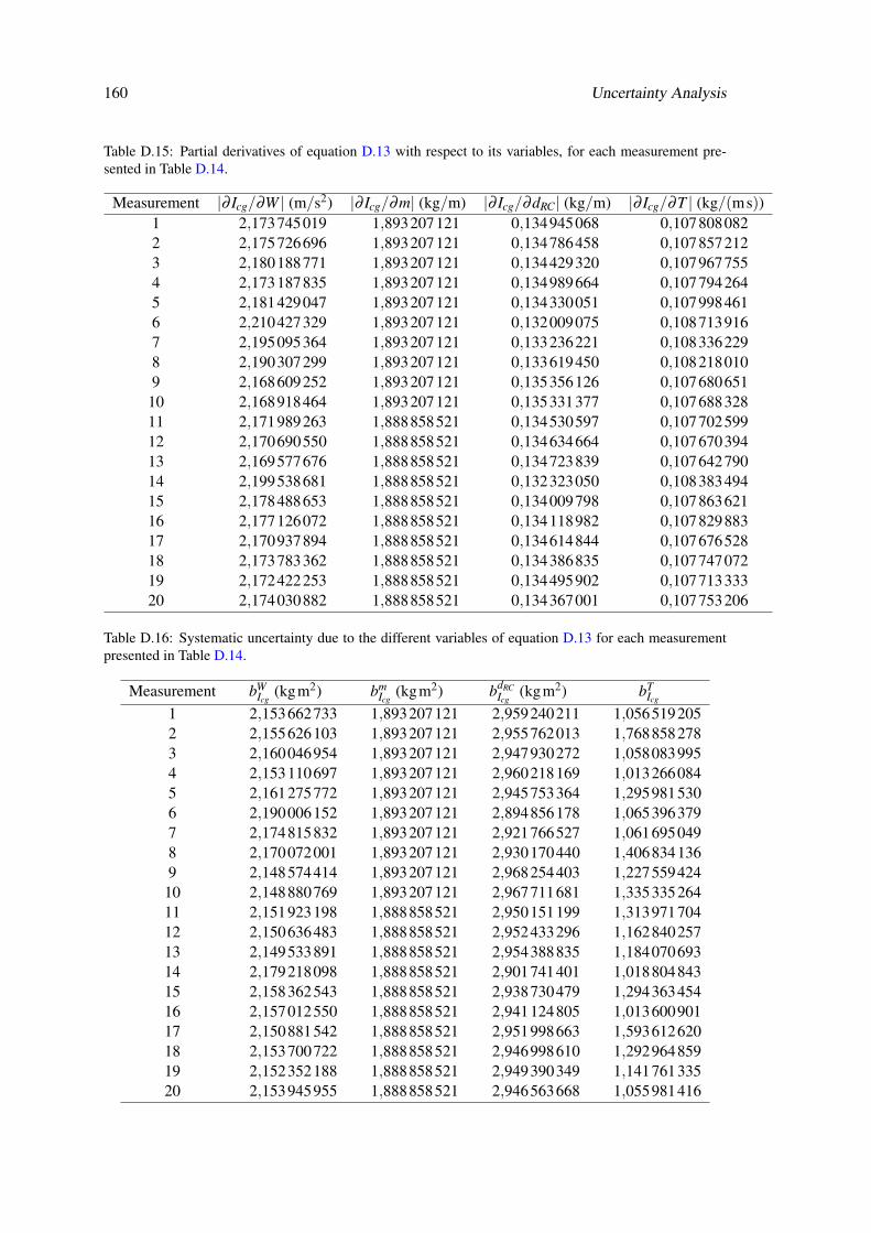
160 Uncertainty Analysis
Table D.15: Partial derivatives of equation D.13 with respect to its variables, for each measurement pre-sented in Table D.14.
Measurement |∂ Icg/∂W | (m/s2) |∂ Icg/∂m| (kg/m) |∂ Icg/∂dRC| (kg/m) |∂ Icg/∂T | (kg/(ms))1 2,173745019 1,893207121 0,134945068 0,1078080822 2,175726696 1,893207121 0,134786458 0,1078572123 2,180188771 1,893207121 0,134429320 0,1079677554 2,173187835 1,893207121 0,134989664 0,1077942645 2,181429047 1,893207121 0,134330051 0,1079984616 2,210427329 1,893207121 0,132009075 0,1087139167 2,195095364 1,893207121 0,133236221 0,1083362298 2,190307299 1,893207121 0,133619450 0,1082180109 2,168609252 1,893207121 0,135356126 0,10768065110 2,168918464 1,893207121 0,135331377 0,10768832811 2,171989263 1,888858521 0,134530597 0,10770259912 2,170690550 1,888858521 0,134634664 0,10767039413 2,169577676 1,888858521 0,134723839 0,10764279014 2,199538681 1,888858521 0,132323050 0,10838349415 2,178488653 1,888858521 0,134009798 0,10786362116 2,177126072 1,888858521 0,134118982 0,10782988317 2,170937894 1,888858521 0,134614844 0,10767652818 2,173783362 1,888858521 0,134386835 0,10774707219 2,172422253 1,888858521 0,134495902 0,10771333320 2,174030882 1,888858521 0,134367001 0,107753206
Table D.16: Systematic uncertainty due to the different variables of equation D.13 for each measurementpresented in Table D.14.
Measurement bWIcg
(kgm2) bmIcg
(kgm2) bdRCIcg
(kgm2) bTIcg
1 2,153662733 1,893207121 2,959240211 1,0565192052 2,155626103 1,893207121 2,955762013 1,7688582783 2,160046954 1,893207121 2,947930272 1,0580839954 2,153110697 1,893207121 2,960218169 1,0132660845 2,161275772 1,893207121 2,945753364 1,2959815306 2,190006152 1,893207121 2,894856178 1,0653963797 2,174815832 1,893207121 2,921766527 1,0616950498 2,170072001 1,893207121 2,930170440 1,4068341369 2,148574414 1,893207121 2,968254403 1,22755942410 2,148880769 1,893207121 2,967711681 1,33533526411 2,151923198 1,888858521 2,950151199 1,31397170412 2,150636483 1,888858521 2,952433296 1,16284025713 2,149533891 1,888858521 2,954388835 1,18407069314 2,179218098 1,888858521 2,901741401 1,01880484315 2,158362543 1,888858521 2,938730479 1,29436345416 2,157012550 1,888858521 2,941124805 1,01360090117 2,150881542 1,888858521 2,951998663 1,59361262018 2,153700722 1,888858521 2,946998610 1,29296485919 2,152352188 1,888858521 2,949390349 1,14176133520 2,153945955 1,888858521 2,946563668 1,055981416

D.6 Determination of the Moment of Inertia 161
Table D.17: Estimation of the uncertainty in moment of inertia through the centre of gravity of the buoy.
Parameter ValueIcg (kgm2) 0,874651797bIcg (kgm2) 0,007138529sIcg (kgm2) 0,038251001sIcg
(kgm2) 0,008553184uIcg (kgm2) 0,011140716t95%ycg 2U95%ycg (kgm2) 0,022281432

162 Uncertainty Analysis
D.7 Clumpweights
The submerged weight of the clumpweights was determined using a Jolly-type scale, with an
expanded uncertainty of U95% = 0,0001 kgf or 0,000981 N which is rounded to 0,001 N. The dry
mass was determined in a scale with an expanded uncertainty of U95% = 0,001kg. These results
are summarised in Table D.18
Table D.18: Uncertainty in the mass and submerged weight of the clumpweights.
Mass (kg) Submerged weight (N)W1 1,115±0,001 9,968±0,001W2 1,125±0,001 10,051±0,001W3 1,113±0,001 9,959±0,001
D.8 Floaters
D.8.1 Diameter
The diameter, DFi, of the floaters was determined indirectly from five measurements of the perime-
ter, PFi, Table D.19 assuming the floaters to be perfect spheres:
DFi = PFi/π (D.16)
The uncertainty in the diameter of the floaters was then determined by propagating the uncer-
tainty in the measurements of the perimeter to the diameter, Tables D.20 to D.21.
Table D.19: Measurements of the perimeter of the floaters.
Measurement PF1(m) PF2(m) PF3(m)1 0,4230 0,4270 0,42002 0,4220 0,4220 0,42503 0,4280 0,4240 0,42704 0,4210 0,4245 0,42055 0,4190 0,4205 0,4205bP ±0,0005
D.8 Floaters 163
Table D.20: Partial derivatives of equation D.16 with respect to its variables, for each measurement pre-sented in Table D.19.
Measurement ∂DF1/∂PF1 ∂DF2/∂PF2 ∂DF3/∂PF3
1 0,134645082 0,135918321 0,1336901522 0,134326772 0,134326772 0,1352817023 0,136236631 0,134963392 0,1359183214 0,134008462 0,135122547 0,1338493075 0,133371842 0,133849307 0,133849307
bDF 0,000159155
Table D.21: Uncertainty in the diameter of the floaters.
Parameter F1 F2 F3DF(m) 0,134517758 0,134836068 0,134517758bDF (m) 0,000159155 0,000159155 0,000159155sDF (m) 0,001070014 0,000790986 0,001015354sDF
(m) 0,000478525 0,000353740 0,000454080uDF (m) 0,000504298 0,000387894 0,000481164t95% 2,776UDF95% (m) 0,001399930 0,001076794 0,001335712
D.8.2 Mass and Buoyancy
The mass of the floaters was measured directly with a scale and is presented in Table D.22, so
uncertainty is that of the scale.
Table D.22: Mass of the floaters and respective uncertainty.
Mass (kg)F1 0,252±0,001F2 0,276±0,001F3 0,232±0,001
The buoyancy of the floaters and its uncertainty were measured as indicated in section C.6 and
are presented in Table D.23
Table D.23: Buoyancy of the floaters and respective uncertainty.
Buoyancy (N)F1 9,97±0,06F2 10,05±0,06F3 9,96±0,06

164 Uncertainty Analysis
D.9 Chain and Cable Properties
D.9.1 Mass and Submerged Weight per Unit Length
The mass per unit length ml and the submerged weight per unit length γl of the chain and of the
synthetic cable were obtained my dividing the mass mc and the submerged weight γc of samples
by their length l:
ml = mc/l (D.17)
γl = γc/l (D.18)
The uncertainty in the mass per unit length ml and in the submerged weight per unit length γl
were then determined by propagating the uncertainty in the measurements.
Ten samples were used to determine the uncertainty in the of the mass per unit length of the
chain, Tables D.24 to D.27, while only five were used to determine its submerged weight per unit
length, Tables D.28 to D.31.
In the case of the synthetic cable, since it was extremely lightweight, it was not feasible to use
several samples. Instead, a single long sample was used, heavy enough for the scales to measure its
mass and submerged weight without significant error and long enough for it to be representative.
The results are presented in Table D.32.
Table D.24: Measurement of the mass and length of 10 samples of chain.
Sample l (m) mc (kg) ml (kg)1 1,0005 0,1456 0,1455272362 1,0000 0,1452 0,1452000003 1,0050 0,1448 0,1440796024 0,9995 0,1448 0,1448724365 1,0000 0,1450 0,1450000006 1,0015 0,1449 0,1446829767 1,0035 0,1452 0,1446935728 1,0030 0,1448 0,1443668999 1,0025 0,1444 0,14403990010 0,9995 0,1446 0,144672336bX 0,0005 0,0001 -

D.9 Chain and Cable Properties 165
Table D.25: Partial derivatives of equation D.18 with respect to its variables, for each measurement pre-sented in Table D.24.
Sample ∂ml/∂mc (m−1) ∂ml/∂ l (kg)1 0,999500250 0,1454545092 1,000000000 0,1452000003 0,995024876 0,1433627884 1,000500250 0,1449449095 1,000000000 0,1450000006 0,998502247 0,1444662767 0,996512207 0,1441889118 0,997008973 0,1439350949 0,997506234 0,14368069910 1,000500250 0,144744709
Table D.26: Systematic uncertainty due to the different variables of equation D.18 for each measurementpresented in Table D.24.
Sample bmcml
(kg) blml
(m) bml (kg/m)1 0,000499750 0,000014545 0,0004999622 0,000500000 0,000014520 0,0005002113 0,000497512 0,000014336 0,0004977194 0,000500250 0,000014494 0,0005004605 0,000500000 0,000014500 0,0005002106 0,000499251 0,000014447 0,0004994607 0,000498256 0,000014419 0,0004984658 0,000498504 0,000014394 0,0004987129 0,000498753 0,000014368 0,00049896010 0,000500250 0,000014474 0,000500459
Table D.27: Estimation of the uncertainty in the mass per unit length of the chain.
Parameter Valueml (kg/m) 0,144713496sml (kg/m) 0,000469623sml (kg/m) 0,000148508bml (kg/m) 0,000157944uml (kg/m) 0,000216797t95% 2Uml95% (kg/m) 0,000433594
Table D.28: Measurement of the submerged weight and length of 5 samples of chain.
Sample l (m) γc (N) γl (N/m)1 1,0010 1,242927 1,2416853152 1,0020 1,244889 1,2424041923 1,0005 1,248813 1,2481889064 0,9995 1,244889 1,2455117565 1,0035 1,242927 1,238591928
bX 0,0005 0,000981 -

166 Uncertainty Analysis
Table D.29: Partial derivatives of equation D.18 with respect to its variables, for each measurement pre-sented in Table D.28.
Sample ∂γl/∂γc (N−1) ∂γl/∂ l (N)1 0,999000999 0,0012404452 0,998003992 0,0012399243 0,999500250 0,0012475654 1,000500250 0,0012461355 0,996512207 0,001234272
Table D.30: Systematic uncertainty due to the different variables of equation D.18 for each measurementpresented in Table D.28.
Sample bγcγl (N/m) bl
γl(N/m) bγl (N/m)
1 0,000499500 0,000001217 0,0004995022 0,000499002 0,000001216 0,0004990033 0,000499750 0,000001224 0,0004997524 0,000500250 0,000001222 0,0005002525 0,000498256 0,000001211 0,000498258
Table D.31: Estimation of the uncertainty in the submerged weight per unit length of the chain.
Parameter Valueγ l (kg/m) 1,243276419sγl (kg/m) 0,003686669sγl(kg/m) 0,001648728bγl(kg/m) 0,000223318uγl(kg/m) 0,001663784tγl95% 2,776Uγl95%(kg/m) 0,004619404
Table D.32: Estimation of the uncertainty in the mass and submerged weight per unit length of the syntheticcable.
Parameter Valuel (m) 5,980±0,001mc (kg) 0,0189±0,0001γc (N) 0,0481±0,0001uml = bml =Uml95% (kg/m) 0,0000170uγl = bγl =Uγl95% (N/m) 0,0001666

D.9 Chain and Cable Properties 167
D.9.2 Dimensions of the Chain
Ten chain links were used to estimate the representative dimensions of the chain. The measure-
ments are presented in Table D.33 and the uncertainty estimates are presented in Table D.34.
Table D.33: Measurements of the dimensions of 10 samples of chain links.
Sample Inner length (m) Inner height (m) Thickness (m)1 0,0205 0,0055 0,00302 0,0209 0,0057 0,00303 0,0207 0,0059 0,00314 0,0204 0,0059 0,00305 0,0208 0,0058 0,00306 0,0208 0,0056 0,00307 0,0206 0,0057 0,00308 0,0206 0,0059 0,00299 0,0206 0,0057 0,002910 0,0205 0,0055 0,0030
Table D.34: Estimation of the uncertainty in the dimensions of the chain links. X represents each of thethree dimensions analysed.
Parameter Inner length Inner height ThicknessX (m) 0,02064 0,00572 0,00299sX (m) 0,00016 0,00015 0,00006sX (m) 0,00005 0,00005 0,00002bX (m) 0,00005uX (m) 0,00007 0,00007 0,00005tX95% 2,262UX95% (m) 0,00011 0,00011 0,00004
D.9.3 Stiffness
As the laboratories of the Faculty of Engineering of the University of Porto could only execute
tensile tests on rigid materials, the determination of the stiffness of the chain and of the synthetic
cable was requested to an independent laboratory. Due to the lack of experience of that laboratory
on testing cables, there were problems during the tests and inconsistencies in the reported results.
Firstly, there is a large variability in the breaking loads of the samples. Secondly, at least two
different values of the length of the samples have to be used in the determination of the stiffness:
the value in the official report and the value in the unofficial notes of each test, Table D.35. The
consequence is that the stiffness results are highly unreliable and must be seen as indicative.
The stiffness was calculated by determining the slope of the initial portion of the force-
elongation curve of each test sample and then multiplying it by the sample’s length, Table D.36.
The uncertainty estimates are presented in Table D.37.

168 Uncertainty Analysis
Table D.35: Length of the samples as reported officially, lr, and as taken from the test notes, ln.
Synthetic cable Chainlr (m) 0,0700 0,0700ln (m) 0,3775 0,2465
Table D.36: Axial stiffness of the samples of synthetic cable and chain.
EA-ln (N) EA-lr (N)Sample Synthetic cable Chain Synthetic cable Chain
1 137874 1641143 25572 4660452 171298 1153132 31771 3274613 170109 1227905 31550 3486954 187855 2606617 34842 7402165 146502 1585530 27172 450252
Table D.37: Uncertainty estimates in the stiffness of the synthetic cable and of the chain.
Parameter Value ln Value lrSynthetic cable Chain Synthetic cable Chain
EA (N) 162728 1642865 30181 466534sEA (N) 20250 579685 3756 164616sEA = uEA (N) 9056 259243 1680 73619t95% 2,776U95% (N) 25140 719658 4663 204365

D.10 Oscillation Periods 169
D.10 Oscillation Periods
The resonance periods of the different degrees of freedom of the buoy were estimated from the
recorded displacement during the decay tests. For each test run it was measured the time span
between the first and the last crest of the displacement, which was then divided by the number of
complete cycles encompassed by that time span. This was repeated for the troughs, providing two
average oscillation periods for each test run.
The uncertainty in the time span ∆ti of test i is the combination of, respectively, the uncer-
tainty in the values of the start, tstart, and finishing time, tfinish, instants, equation D.20, while the
uncertainty in each measured period Ti, is the uncertainty in the time span divided by the number
of oscillations, equation D.20:
u∆ti =√
ut2start
+ut2finish
(D.19)
uTi =√
ut2start
+ut2finish
/N (D.20)
where N is the number of oscillations.
The uncertainty in the value of the time instants is at most half of the value of the acquisition
period, which, for the acquisition period of 0,01 s used in the experiments, is 0,005 s. So, the
systematic uncertainty for each individual time span measured is always 0,0070710678 s. The
minimum number of cycles recorded (which sets the maximum limit for the systematic uncertainty
in the resonance period) is 3, resulting in a systematic uncertainty of 0,0023570227 s.
The results of the measured resonance periods and respective uncertainties for the four config-
urations tested in surge, heave and pitch are presented in Tables D.38 to D.59.

170 Uncertainty Analysis
Table D.38: Measured heave resonance periods for the free buoy.
Sample Ti−crest (s) Ti−trough (s)1 1,104016 1,1065192 1,104307 1,0975903 1,112994 1,1208424 1,111026 1,1104265 1,109427 1,1187536 1,106851 1,1012867 1,105955 1,1039528 1,115628 1,1080229 1,100137 1,10131510 1,126604 1,12382111 1,127088 1,13056412 1,123439 1,11782513 1,115760 1,10100314 1,118023 1,11792115 1,128684 1,12748316 1,117765 1,11514817 1,103160 1,10065318 1,100802 1,09041219 1,132639 1,12521220 1,106823 1,11886521 1,104750 1,110843
Table D.39: Estimated heave resonance period and uncertainty for the free buoy.
Parameter ValueT (s) 1,112484119sT (s) 0,010355250sT (s) 0,001597850bT (s) 0,002357023uT (s) 0,002847574t95% 2UT 95% (s) 0,005695149

D.10 Oscillation Periods 171
Table D.40: Measured pitch resonance periods for the free buoy.
Sample Ti−crest (s) Ti−trough (s)1 1,168848 1,1690572 1,169153 1,1686443 1,168855 1,1695174 1,170263 1,1714085 1,169383 1,1688536 1,167181 1,1686187 1,167652 1,1701908 1,171605 1,1707049 1,174000 1,17243710 1,171132 1,17154411 1,169527 1,16952812 1,167881 1,16737313 1,169291 1,16978414 1,167593 1,16763215 1,169468 1,17049216 1,169784 1,17207017 1,174548 1,17257118 1,170406 1,17046519 1,171279 1,169707
Table D.41: Estimated pitch resonance period and uncertainty for the free buoy.
Parameter ValueT (s) 1,169959026sT (s) 0,001740804sT (s) 0,000282396bT (s) 0,002357023uT (s) 0,002373879tT 95% 2UT 95% (s) 0,004747759
Table D.42: Measured surge resonance periods for CON1.
Sample Ti−crest (s) Ti−trough (s)1 8,558512 8,5652642 8,544674 8,5529323 8,549998 8,5478664 8,558597 8,5613495 8,559936 8,5652766 8,561259 8,5602227 8,564380 8,5513938 8,561270 8,5664969 8,553642 8,56541310 8,557869 8,55832111 8,579183 8,55234612 8,568646 8,57271913 8,577044 8,583961

172 Uncertainty Analysis
Table D.43: Estimated surge resonance period and uncertainty for CON1.
Parameter ValueT (s) 8,561483385sT (s) 0,009549823sT (s) 0,001872874bT (s) 0,002357023uT (s) 0,003010517t95% 2UT 95% (s) 0,006021035
Table D.44: Measured heave resonance periods for CON1.
Sample Ti−crest (s) Ti−trough (s)1 1,096024 1,1042962 1,131259 1,1281693 1,112264 1,1037304 1,145035 1,1874815 1,135861 1,1188406 1,117670 1,1211267 1,157403 1,1330418 1,132073 1,1358609 1,108991 1,11975510 1,113527 1,10445311 1,116026 1,11567612 1,111145 1,11629913 1,090694 1,07088214 1,112049 1,10477615 1,095777 1,10000916 1,117793 1,11919117 1,102488 1,09951318 1,121274 1,133295
Table D.45: Estimated heave resonance period and uncertainty for CON1.
Parameter ValueT (s) 1,117604028sT (s) 0,020377729sT (s) 0,003396288bT (s) 0,002357023uT (s) 0,004134045tT 95% 2UT 95% (s) 0,008268090

D.10 Oscillation Periods 173
Table D.46: Measured pitch resonance periods for CON1.
Sample Ti−crest (s) Ti−trough (s)1 1,145093 1,1443662 1,147032 1,1467933 1,141374 1,1405304 1,144999 1,1450365 1,144724 1,1445626 1,145513 1,1454747 1,144190 1,1445128 1,149224 1,1503029 1,148573 1,14975810 1,145389 1,14536411 1,142512 1,14195312 1,142302 1,14233113 1,143963 1,14432514 1,144554 1,14512415 1,145469 1,14609816 1,150212 1,15172817 1,147221 1,14747618 1,143900 1,14372619 1,143823 1,145036
Table D.47: Estimated pitch resonance period and uncertainty for CON1.
Parameter ValueT (s) 1,145383184sT (s) 0,002543456sT (s) 0,000412603bT (s) 0,002357023uT (s) 0,002392864t95% 2UT 95% (s) 0,004785728
174 Uncertainty Analysis
Table D.48: Measured surge resonance periods for CON2.
Sample Ti−crest (s) Ti−trough (s)1 8,092495 8,2302332 9,281521 9,2781303 8,929140 8,9183934 9,285090 9,2855645 9,283016 9,2875026 9,278361 9,2804737 9,283872 9,2843108 9,278250 9,2870159 9,275347 9,28924210 9,281112 9,29188211 9,280400 9,29085112 9,288295 9,28434413 9,287495 9,28990814 9,281317 9,28997215 9,284420 9,28709516 9,285582 9,28533617 9,279306 9,29533218 9,262891 9,26307119 9,273627 9,26623520 9,279655 9,28776321 9,275559 9,27828822 9,275014 9,283079
Table D.49: Estimated surge resonance period and uncertainty for CON2.
Parameter ValueT (s) 9,214904159sT (s) 0,245034969sT (s) 0,037809717bT (s) 0,002357023uT (s) 0,037883113t95% 2UT 95% (s) 0,075766225

D.10 Oscillation Periods 175
Table D.50: Measured heave resonance periods for CON2.
Sample Ti−crest (s) Ti−trough (s)1 1,131091 1,1324902 1,168234 1,1683013 1,145988 1,1461964 1,138877 1,1338665 1,114005 1,1147346 1,136298 1,1310277 1,147686 1,1359988 1,127448 1,1256819 1,141449 1,13719910 1,137681 1,13378511 1,123963 1,12482612 1,137103 1,13619713 1,126965 1,12790714 1,124734 1,12834715 1,126756 1,13271116 1,134966 1,13241217 1,133840 1,12652418 1,132592 1,13375619 1,145080 1,13764620 1,131713 1,13480521 1,117647 1,12295122 1,125938 1,12787023 1,121623 1,12438824 1,116095 1,120372
Table D.51: Estimated heave resonance period and uncertainty for CON2.
Parameter ValueT (s) 1,132453354sT (s) 0,010948425sT (s) 0,001580269bT (s) 0,002357023uT (s) 0,002837747t95% (s) 2UT 95% (s) 0,005675493

176 Uncertainty Analysis
Table D.52: Measured pitch resonance periods for CON2.
Sample Ti−crest (s) Ti−trough (s)1 1,169787 1,1686702 1,171517 1,1718463 1,172021 1,1720154 1,156619 1,1575695 1,168642 1,1679726 1,163188 1,1638437 1,171503 1,1721508 1,167627 1,1677249 1,171052 1,17088110 1,169115 1,17023611 1,162492 1,16110612 1,170392 1,17001113 1,171019 1,16880914 1,173042 1,17399815 1,170888 1,17120216 1,165168 1,16482217 1,167877 1,16695518 1,168271 1,16775919 1,161730 1,16210720 1,163626 1,16272821 1,171278 1,170808
Table D.53: Estimated pitch resonance period and uncertainty for CON2.
Parameter ValueT (s) 1,167858690sT (s) 0,004223476sT (s) 0,000651696bT (s) 0,002357023uT (s) 0,002445458t95% 2UT 95% (s) 0,004890916

D.10 Oscillation Periods 177
Table D.54: Measured surge resonance periods for the catenary.
Sample Ti−crest (s) Ti−trough (s)1 9,078914 9,0783062 9,063779 9,0910573 9,093684 9,1009184 9,075638 9,0880495 9,187799 9,1837556 9,086606 9,1203377 9,093328 9,1205628 9,121051 9,1442849 9,118352 9,13682710 9,188068 9,21437311 9,086606 9,12033712 9,128758 9,14263313 9,135614 9,15426114 9,107804 9,14382315 9,106242 9,15613516 9,181829 9,21394917 9,173577 9,18491718 9,113824 9,14360119 9,117770 9,14799220 9,131754 9,15798621 9,227472 9,233282
Table D.55: Estimated surge resonance period and uncertainty for the catenary.
Parameter ValueT (s) 9,135615548sT (s) 0,043770031sT (s) 0,006753862bT (s) 0,002357023uT (s) 0,007153336t95% 2UT 95% (s) 0,014306671

178 Uncertainty Analysis
Table D.56: Measured heave resonance periods for the catenary.
Sample Ti−crest (s) Ti−trough (s)1 1,148662 1,1427752 1,126058 1,1198803 1,156484 1,1600234 1,137993 1,1340085 1,125456 1,1192116 1,103790 1,0962907 1,102856 1,1006528 1,110291 1,1095629 1,136071 1,14979910 1,143903 1,14871811 1,141938 1,14131212 1,151259 1,14859513 1,150070 1,13427714 1,094876 1,102907
Table D.57: Estimated heave resonance period and uncertainty for the catenary.
Parameter ValueT (s) 1,129918429sT (s) 0,020281486sT (s) 0,003832841bT (s) 0,002357023uT (s) 0,004499580t95% 2U95% (s) 0,008999161

D.10 Oscillation Periods 179
Table D.58: Measured pitch resonance periods for the catenary.
Sample Ti−crest (s) Ti−trough (s)1 1,166812 1,1655022 1,171127 1,1704623 1,171148 1,1695264 1,160866 1,1618345 1,170053 1,1702636 1,119962 1,1288017 1,161589 1,1616288 1,162648 1,1626609 1,174684 1,17692810 1,163983 1,16669611 1,145374 1,14505412 1,162738 1,16822513 1,161108 1,15889214 1,173560 1,17385415 1,171523 1,17111716 1,159885 1,16127117 1,166628 1,16936718 1,164262 1,16457719 1,158938 1,15729920 1,155988 1,15809521 1,170400 1,17064222 1,168210 1,16942323 1,159135 1,16073824 1,169065 1,16710125 1,162312 1,164247
Table D.59: Estimated pitch resonance period and uncertainty for the catenary.
Parameter ValueT (s) 1,163324000sT (s) 0,010325421sT (s) 0,001593247bT (s) 0,002357023uT (s) 0,002844994t95% 2UT 95% (s) 0,005689988

180 Uncertainty Analysis
D.11 Load Cells
The mass of the load cells, including accessories, was measured using a scale with an uncertainty
of 0,0001 kg, Table D.60.
Table D.60: Mass of the load cells.
Load cell Mass (kg)LC1 0,0131LC2 0,0141
The reference value adopted for the mass of the load cells was the largest one 0,0141 kg,
as this is the value that would cause the largest difference between the real and the theoretical
measurements.
D.12 Load Cell Attachments
The mass of the load cell adapters was measured using a scale with an uncertainty of 0,0001 kg,
Table D.61. Since there were four different adapters, the average value of the mass and associated
uncertainty was estimated, Table D.62.
Table D.61: Mass of the load cell adapters.
Adapter Mass (kg)1 0,05612 0,05903 0,05644 0,0571
Table D.62: Average value and uncertainty of the mass of the load cell adapters.
Parameter Valuemadap (kg) 0,05715bm−adap (kg) 0,00010sm−adap (kg) 0,00130sm−adap (kg) 0,00065t95% 3,182um−adap (kg) 0,00066Um−adap95% (kg) 0,00210

D.13 Draft 181
D.13 Draft
The draft, db, was estimated indirectly by subtracting readings of the freeboard, f , on four points
around the perimeter of the buoy from its height, Hb, Figure D.2 and equation D.21:
f
db
Hb
Figure D.2: Variables in the determination of the draft.
db = Hb− f (D.21)
The measured values of the freeboard, the calculated values of the draft and its uncertainty for
the four configurations tested are presented in Tables D.63 to D.70.
Table D.63: Freeboard and draft of the free buoy.
f (m) db (m)0,2235 0,17700,2255 0,17500,2255 0,17500,2225 0,1780
Table D.64: Uncertainty in the draft for the free buoy.
Parameter Valueb f (m) 0,00050uHb(m) 0,00065db(m) 0,17625sdb(m) 0,00150sdb
(m) 0,00075udb(m) 0,00111t95% 3,182Udb95%(m) 0,00353

182 Uncertainty Analysis
Table D.65: Freeboard and draft of the buoy in CON1.
f (m) db (m)0,2260 0,17450,2220 0,17850,2215 0,17900,2240 0,1765
Table D.66: Uncertainty in the draft of the buoy in CON1.
Parameter Valueb f (m) 0,00050uHb(m) 0,00065db(m) 0,17713sdb(m) 0,00206sdb
(m) 0,00103udb(m) 0,00131t95% 3,182Udb95%(m) 0,00418
Table D.67: Freeboard and draft of the buoy in CON2.
f (m) db (m)0,2140 0,18650,2120 0,18850,2100 0,19050,2110 0,1895
Table D.68: Uncertainty in the draft of the buoy in CON2.
Parameter Valueb f (m) 0,00050uHb(m) 0,00065db(m) 0,18875sdb(m) 0,00171sdb
(m) 0,00085udb(m) 0,00118t95% 3,182UHb95%(m) 0,00376
Table D.69: Freeboard and draft of the buoy moored with the catenary.
f (m) db (m)0,2240 0,17650,2190 0,18150,2180 0,18250,2200 0,1810

D.13 Draft 183
Table D.70: Uncertainty in the draft of the buoy moored with the catenary.
Parameter Valueb f (m) 0,00050udb(m) 0,00065db(m) 0,18036sdb(m) 0,00265sdb
(m) 0,00133uHb(m) 0,00156t95% 3,182Udb95%(m) 0,00496

184 Uncertainty Analysis
D.14 Calibration Errors
The quantification of the uncertainty associated with calibrations is more involved than the analy-
ses executed in the previous sections. To simplify the analysis, it is necessary to evaluate the error
sources, which are:
• the systematic uncertainty in the applied loads (load cells) or displacements (wave probes);
• the random noise in the records;
• the systematic uncertainty caused by the signal conditioning and analogue-to-digital con-
version.
Taking into account the error sources, the following assumptions were made:
• in the calibration, there is no random uncertainty in the voltage readings, since each reading
was the result of averaging 3000 samples, recorded for 30 s at 100 Hz;
• the systematic errors caused by the signal conditioning and by the analogue-to-digital con-
version in the experiments are the same as during calibration (there was no change to the
system) and so they cancel out;
• there is random uncertainty in the measurements during the experiments due to the noise
in the records, which is quantified by the largest standard deviation of the voltage readings
during calibration;
• all calibration points have the same systematic error magnitude, which is equal to largest
systematic error determined for the loads or displacements.
The conversion of the voltage readings to force and free surface elevation was made using a
straight line estimated by a least squares fit to the calibration points:
Y = mV +b (D.22)
where V is the voltage reading, m and b are the slope and constant of the straight line determined in
the least squares fit and Y is the force or surface elevation value. In these conditions, the evaluation
of the uncertainty due to the use of a least squares fit is given by:
uY =
√u2
Y−fit +
(∂Y∂V
)2
s2V (D.23)
where sV is the random uncertainty in the voltage and uY−fit is given by

D.14 Calibration Errors 185
uY−fit =
√√√√s2Y
(1N+
(V −V
)2
sVV
)(D.24)
sY =
√∑
Ni=1 (Yi−mVi− c)2
N−2(D.25)
sVV =N
∑i=1
X2i −
(∑
Ni=1Vi
)2
N(D.26)
where Vi is the voltage reading of calibration point i from a total number N of calibration points.
The uncertainty due to the fit is then combined with the random and systematic uncertainties in Y
and V just like what was done in the previous sections.
D.14.1 Calibration of the Wave Probes
The conversion of voltage to water surface elevation is given by equation D.27:
η = mV +b (D.27)
where η is the water surface elevation. The systematic uncertainty in η is bη = 0,00001m. Since
only three points were used in the calibration of the wave probes, the value of t95% is 12,706.
The parameters of each wave probe calibration are given in Table D.71, while the intermediate
calculations of the uncertainty and the final results are given in Tables D.72 and D.73.

186 Uncertainty Analysis
Table D.71: Parameters of the least squares fit for each calibration of the wave probes.
Calibration m (m/V) b (m) R2
cal-12-08-2014 0,028873668 −0,002797314 0,999999125cal-13-08-2014 0,029254055 −0,002193480 0,999994582cal-14-08-2014 0,028308565 −0,001855990 0,999998343cal-18-08-2014 0,029330360 −0,002604095 0,999995200cal-19-08-2014 0,028218085 −0,003203104 0,999996469cal-20-08-2014 0,028081371 −0,002063971 0,999972101cal-21-08-2014 0,028212225 −0,002588976 0,999998470cal-22-08-2014 0,028017494 −0,003258077 0,999999422cal-25-08-2014 0,027997092 −0,003300376 0,999964583cal-26-08-2014-2 0,028076652 −0,002958296 0,999963086cal-27-08-2014 0,028365268 −0,001964357 0,999997834cal-28-08-2014 0,028178137 −0,002949667 0,999999633cal-29-08-2014 0,027978028 −0,002303572 0,999983719cal-01-09-2014 0,027557723 −0,003043433 0,999967239cal-02-09-2014 0,027864629 −0,001985979 0,999978493cal-03-09-2014 0,028011992 −0,002320114 0,999992076cal-05-09-2014 0,027907459 −0,002285613 0,999990430cal-08-09-2014 0,027982975 −0,002710427 0,999986506cal-09-09-2014 0,028537199 −0,002429117 0,999972351cal-10-09-2014 0,027829204 −0,003015434 0,999971187cal-11-09-2014 0,028720279 −0,002672915 0,999977131cal-12-09-2014 0,028567063 −0,002881163 0,999998640cal-15-09-2014 0,027118183 −0,003076058 0,999925292cal-16-09-2014 0,027455177 −0,002368326 0,999978512cal-17-09-2014 0,027604804 −0,002903947 0,999987649

D.14 Calibration Errors 187
Table D.72: Parameters for the estimation of the uncertainty in the wave probe calibration due to the leastsquares fit.
Calibration uη−fit (m) sV (V) ∂η/∂V × sV (m)cal-12-08-2014 0,000052926 0,016938302 0,000489071cal-13-08-2014 0,000131672 0,019179370 0,000561074cal-14-08-2014 0,000072818 0,016315949 0,000461881cal-18-08-2014 0,000123942 0,016055628 0,000470917cal-19-08-2014 0,000106292 0,016393480 0,000462593cal-20-08-2014 0,000298792 0,015511748 0,000435591cal-21-08-2014 0,000069977 0,016218185 0,000457551cal-22-08-2014 0,000043018 0,016231172 0,000454757cal-25-08-2014 0,000336651 0,017572773 0,000491987cal-26-08-2014-2 0,000343694 0,016135106 0,000453020cal-27-08-2014 0,000083249 0,015453967 0,000438356cal-28-08-2014 0,000034290 0,015655376 0,000441139cal-29-08-2014 0,000228255 0,015878988 0,000444263cal-01-09-2014 0,000323785 0,015348027 0,000422957cal-02-09-2014 0,000262341 0,014659314 0,000408476cal-03-09-2014 0,000159239 0,014416403 0,000403832cal-05-09-2014 0,000174996 0,015005468 0,000418765cal-08-09-2014 0,000207801 0,015454355 0,000432459cal-09-09-2014 0,000297449 0,016249709 0,000463721cal-10-09-2014 0,000303649 0,015271369 0,000424990cal-11-09-2014 0,000270517 0,015601780 0,000448087cal-12-09-2014 0,000065980 0,016221301 0,000463395cal-15-09-2014 0,000488942 0,007887581 0,000213897cal-16-09-2014 0,000262227 0,008768118 0,000240730cal-17-09-2014 0,000198803 0,009346030 0,000257995

188 Uncertainty Analysis
Table D.73: Estimate of the uncertainty in the calibration of the wave probes.
Calibration uη (m) Uη95% (m)cal-12-08-2014 0,000492028 0,006251708cal-13-08-2014 0,000576404 0,007323792cal-14-08-2014 0,000467693 0,005942506cal-18-08-2014 0,000487057 0,006188548cal-19-08-2014 0,000474752 0,006032204cal-20-08-2014 0,000528315 0,006712764cal-21-08-2014 0,000462979 0,005882614cal-22-08-2014 0,000456896 0,005805325cal-25-08-2014 0,000596225 0,007575638cal-26-08-2014-2 0,000568729 0,007226269cal-27-08-2014 0,000446303 0,005670725cal-28-08-2014 0,000442583 0,005623459cal-29-08-2014 0,000499569 0,006347529cal-01-09-2014 0,000532756 0,006769198cal-02-09-2014 0,000485568 0,006169623cal-03-09-2014 0,000434209 0,005517062cal-05-09-2014 0,000453968 0,005768123cal-08-09-2014 0,000479898 0,006097583cal-09-09-2014 0,000551011 0,007001145cal-10-09-2014 0,000522417 0,006637828cal-11-09-2014 0,000523509 0,006651710cal-12-09-2014 0,000468175 0,005948637cal-15-09-2014 0,000533775 0,006782150cal-16-09-2014 0,000356110 0,004524728cal-17-09-2014 0,000325859 0,004140367

D.14 Calibration Errors 189
D.14.2 Calibration of the Load Cells
The conversion of voltage to water surface elevation is given by equation D.28:
τ = mV +b (D.28)
where τ is the tension in the cables. The systematic uncertainty in τ is bτ = 0,000990761N.
Since more than ten points were used in the calibration of the load cells, the value of t95% is set
to 2. The parameters of each load cell calibration are given in Table D.74, while the intermediate
calculations of the uncertainty and the final results are given in Tables D.75 and D.76.
Table D.74: Parameters of the least squares fit for the calibration of the load cells.
Load cell m (N/V) b (N) R2
1 22,250915115 −110,796341390 0,9999990772 22,354139075 −111,700192921 0,999998928
Table D.75: Parameters for the estimation of the uncertainty in the calibration of the load cells due to theleast squares fit.
Load cell uτ−fit (N) sV (V) ∂τ/∂V × sV (N)1 0,034267490 0,004429628 0,0985632842 0,036926675 0,005149398 0,115110360
Table D.76: Estimate of the uncertainty in the calibration of the load cells.
Load cell uτ (N) Uτ95% (N)1 0,104354988 0,2087099752 0,120892331 0,241784663

190 Uncertainty Analysis

Bibliography
[1] J. Fitzgerald. Position Mooring of Wave Energy Converters. Phd thesis, Chalmers Univer-
sity of Technology, 2009.
[2] L. Martinelli, P. Ruol, and G. Cortellazzo. On mooring design of wave energy converters:
the Seabreath application. In P. Lynett and J. McKee Smith, editors, Proceedings of the
33rd International Conference Coastal Engineering (ICCE), pages 1–12, Santander, 2012.
[3] J. Fitzgerald and L. Bergdahl. Including moorings in the assessment of a generic offshore
wave energy converter: A frequency domain approach. Marine Structures, 21(1):23–46,
2008.
[4] W. C. Webster. Mooring-induced damping. Ocean Engineering, 22(6):571–591, 1995.
[5] E. Angelelli, B. Zanuttigh, F. Ferri, and J.P. Kofoed. Experimental assessment of the moor-
ing influence on the power output of floating Wave Activated Body WECs. In P. Frigaard,
J. P. Kofoed, A. S. Bahaj, L. Bergdahl, A. Clément, D. Conley, A. F. O. Falcão, C. M.
Johnstone, L. Margheritini, I. Masters, and D. Sarmento, A. J.and Vicinanza, editors, Pro-
ceedings of the 10th European Wave and Tidal Energy Conference, Aalborg, Denmark,
2013. European Wave and Tidal Energy Conference.
[6] F. Cerveira, N. Fonseca, and R. Pascoal. Mooring system influence on the efficiency of
wave energy converters. International Journal of Marine Energy, 3–4:65 – 81, 2013.
[7] P. C. Vicente, A. F. O. Falcão, and P. A. P. Justino. Optimization of Mooring Configuration
Parameters of Floating Wave Energy Converters. In International Conference on Ocean,
Offshore and Arctic Engineering, OMAE, pages 759–765, Rotterdam, 2011. ASME.
[8] P. C. Vicente, A. F. O. Falcão, and P. A. P. Justino. Non-linear Slack-Mooring Modelling
of a Floating Two-Body Wave Energy Converter. In Proceedings of the 9th European Wave
and Tidal Energy Conference, Southampton, UK, 2011. EWTEC.
[9] L. Johanning, G. H. Smith, and J. Wolfram. Towards Design Standards for WEC Moorings.
In 6th European Wave and Tidal Energy Conference, pages 223–230, Glasgow, UK, 2005.
EWTEC.
191

192 BIBLIOGRAPHY
[10] N. Fonseca, R. Pascoal, T. Morais, and R. Dias. Design of a mooring system with synthetic
ropes for the FLOW wave energy converter. In Proceedings of the ASME 2009 28th Interna-
tional Conference on Ocean, Offshore and Arctic Engineering, volume 4, pages 1189–1198,
Honolulu, HI, United states, 2009. American Society of Mechanical Engineers.
[11] J. Fitzgerald and L. Bergdahl. Considering Mooring Cables for Offshore Wave Energy
Converters. In Proceeding of the 7th European Wave and Tidal Energy Conference, Porto,
2007. IST/IDMEC.
[12] M. Irvine. Cable Structures. Dover Publication, Inc., New York, 1981.
[13] T. S. Walton and H. Polachek. Calculation of transient motion of submerged cables. Math-
ematics of Computation, (14):27–46, 1960.
[14] C. M. Larsen and I. J. Fylling. Dynamic behaviour of anchor lines. Technical Report 3,
Norwegian Maritime Research, 1982.
[15] M. S. Triantafyllou, A. Bliek, and H. Shin. Dynamic Analysis as a Tool for Open-Sea
Mooring System Design. SNAME Transactions, 93:303–324, 1985.
[16] C. M. Ablow and S. Schechter. Numerical simulation of undersea cable dynamics. Ocean
Engineering, 10(6):443–457, 1983.
[17] K. A. Ansari and N. U. Khan. The Effect of Cable Dynamics on the Station-Keeping Re-
sponse of a Moored Offshore Vessel. Journal of Energy Resources Technology, 108(1):52–
58, 1986.
[18] J. W. Leonard and J. H. Nath. Comparison of finite element and lumped parameter methods
for oceanic cables. Engineering Structures, 3(3):153–167, 1981.
[19] M. Nakamura, W. Koterayama, and Y. Kyozuka. Slow drift damping due to drag forces
acting on mooring lines. Ocean Engineering, 18(4):283–296, 1991.
[20] J. J. Burgess. Equations of Motion of a Submerged Cable with Bending Stiffness. In S. K.
Chakrabarti, C. Sparks, R. C. Ertekin, and S. Jagannathan, editors, Proceedings of the 11th
International Conference on Offshore Mechanics and Artic Engineering, pages 283–289,
Calgary, Alberta, Canada, 1992. ASME.
[21] M. S. Triantafyllou and C. T. Howell. Dynamic Response of Cables Under Negative Ten-
sion: An Ill-Posed Problem. Journal of Sound and Vibrations, 173(4):433–447, 1994.
[22] V. J. Papazoglou, S. A. Mavrakos, and M. S. Triantafyllou. Non-linear cable response and
model testing in water. Journal of Sound and Vibration, 140(1):103–115, 1990.

BIBLIOGRAPHY 193
[23] S. A. Mavrakos, J. Chatjigerorgiou, and V. J. Papazoglou. Use of buoys for dynamic tension
reduction in deep water mooring applications. In Proceedings of the 7th International Con-
ference on the Behavior of Offshore Structures (BOSS’94), pages Vol. 2, 417–426, Boston,
1994. Pergamon.
[24] S. A. Mavrakos, V. J. Papazoglou, M. S. Triantafyllou, and J. Hatjigeorgiou. Deep water
mooring dynamics. Marine Structures, 9(2):181–209, 1996.
[25] L. Johanning, G. H. Smith, and C. Bullen. Large scale mooring line experiments and com-
parison with a fully dynamic simulation program with importance to WEC installation.
pages 455–462, Lisbon, Portugal, 2007. International Society of Offshore and Polar Engi-
neers.
[26] L. Johanning, G. Smith, and J. Wolfram. Measurements of static and dynamic mooring
line damping and their importance for floating WEC devices. Ocean Engineering, 34(14-
15):1918–1934, 2007.
[27] A. Vickers and L. Johanning. Comparison of damping properties for three different mooring
arrangements. In Proceedings of the 8th European Wave and Tidal Conference, pages 637–
645, Uppsala, Sweden, 2009.
[28] O. M. Aamo and T. I. Fossen. Finite Element Modelling of Moored Vessels. Mathemat-
ical and Computer Modelling of Dynamical Systems: Methods, Tools and Applications in
Engineering and Related Sciences, 7(1):47–75, 2001.
[29] R. Pascoal, S. Huang, N. Barltrop, and C. Guedes-Soares. Equivalent force model for the
effect of mooring systems on the horizontal motions. Applied Ocean Research, 27(3):165–
172, 2005.
[30] A. Montano, M. Restelli, and R. Sacco. Numerical simulation of tethered buoy dynamics
using mixed finite elements. Computer Methods in Applied Mechanics and Engineering,
196(41-44):4117–4129, 2007.
[31] D. N. Arnold, F. Brezzi, B. C, and L. D. Marini. Unified Analysis of Discontinuous Galerkin
Methods for Elliptic Problems. SIAM Journal on Numerical Analysis, 39(5):1749–1779,
2002.
[32] B. Cockburn and C.-W. Shu. The Local Discontinuous Galerkin Method for Time-
Dependent Convection-Diffusion Systems. SIAM Journal on Numerical Analysis,
35(6):2240–2463, 1998.
[33] B. Cockburn and C. Shu. Runge–Kutta Discontinuous Galerkin Methods for Convection-
Dominated Problems. Journal of Scientific Computing, 16(3):173–261, 2001.
[34] P. R. Thies, L. Johanning, and G. H. Smith. Towards component reliability testing for
marine energy converters. Ocean Engineering, 38(2–3):360–370, 2011.

194 BIBLIOGRAPHY
[35] G. E. Karniadakis and S. J. Sherwin. Spectral/hp Element Methods for CFD. Oxford
University Press, Oxford, New York, 2nd edition, 2003.
[36] J. S. Hesthaven and T. Warburton. Nodal Discontinuous Galerkin Methods - Algorithms,
Analysis, and Applications. Springer, New York, 2008.
[37] J. N. Newman. Marine Hydrodynamics. The MIT Press, Cambridge, 1977.
[38] O. M. Faltinsen. Sea Loads on Ships and Offshore Structures. Cambridge University Press,
Cambridge, 1993.
[39] Q. W. Ma and S. Yan. QALE-FEM for numerical modelling of non-linear interaction be-
tween 3D moored floating bodies and steep waves. International Journal for Numerical
Methods in Engineering, 78(6):713–756, 2009.
[40] Y.-H. Yu and Y. Li. Preliminary results of a RANS simulation for a floating point absorber
wave energy system under extreme wave conditions. In Proceedings of the ASME 30th
International Conference on Ocean, Offshore and Arctic Engineering OMAE2011, Rother-
dam, The Netherlands, 2011. ASME.
[41] C. Eskilsson, J. Palm, J. P. Kofoed, and E. Friis-Madsen. CFD study of the overtopping
discharge of the Wave Dragon wave energy converter. In Renewable Energies Offshore,
pages 287–294. CRC Press, 2015.
[42] W. E. Cummins. The impulse response function and ship motions. Technical Report 1661,
David Taylor Model Basin Washington D. C., 1962.
[43] G. van Oortmerssen. The Motions of a Moored Ship in Waves. Phd, Delft University of
Technology, 1976.
[44] L. Bergdahl and N. Mårtensson. Certification of Wave-Energy Plants - Discussion of Ex-
isting Guidelines, especially for mooring design. In Second European Wave Power Confer-
ence, Lisbon, 1995.
[45] R. E. Harris, L. Johanning, and J. Wolfram. Mooring systems for wave energy converters: A
review of design issues and choices. In 3rd International Conference on Marine Renewable
Energy, pages 180–189, Blyth, UK, 2004.
[46] Det Norske Veritas. Guidelines on design and operation of wave energy converters. Tech-
nical report, Carbon Trust, 2005.
[47] Det Norske Veritas. Offshore Standard DNV-OS-E301 - Position Mooring, 2004.
[48] Mooring design approach for wave energy converters. Proceedings of the Institution of
Mechanical Engineers, Part M: Journal of Engineering for the Maritime Environment,
220(4):159–174, 2006.

BIBLIOGRAPHY 195
[49] N.D.P. Barltrop. Floating Structures - A Guide for Design and Analysis, Volumes 1-2.
Energy Institute, 1998.
[50] J. Falnes. Ocean Waves and Oscillating Systems Linear Interactions Including Wave-Energy
Extraction. Cambridge University Press, 2002.
[51] N. Fonseca, R. Pascoal, J. Marinho, and T. Morais. Analysis of Wave Drift Forces on a
Floating Wave Energy Converter. In 27th International Conference on Offshore Mechanics
and Arctic Engineering, number 2003, pages 831–839, Estoril, 2008. ASME.
[52] C. Retzler. Measurements of the slow drift dynamics of a model Pelamis wave energy
converter. Renewable Energy, 31(2):257–269, 2006.
[53] W. Sheng, A. W. Lewis, and R. Alcorn. Numerical Investigation into Hydrodynamics of
Moored Floating Wave Energy Converters. In Proceedings of the 10th European Wave and
Tidal Energy Conference, Aalborg, 2013. EWTEC.
[54] Equimar. Protocols for the Equitable Assessment of Marine Energy Converters. The Insti-
tute for Energy Systems, School of Engineering, The University of Edinburgh, Edinburgh,
1st edition, 2011.
[55] C. T. Howell and M. S. Triantafyllou. Stable and Unstable Nonlinear Resonant Response
of Hanging Chains: Theory and Experiment. Proceedings: Mathematical and Physical
Sciences, 440(1909):345–364, 1993.
[56] W. S. Yang. Hydrodynamic Analyis of Mooring Lines Based on Optical Tracking Experi-
ments. Phd, Texas A&M University, 2007.
[57] W. Tomaszewski, P. Pieranski, and J. C. Geminard. The motion of a freely falling chain tip.
American Journal of Physics, 74(9):776–783, 2006.
[58] R. J. Montague, J. Watton, and K. J. Brown. A machine vision measurement of slab camber
in hot strip rolling. Journal of Materials Processing Technology, 168(1):172–180, 2005.
[59] D. C. Brown. Close-range camera calibration. Photogrammetric Engineering, 37(8):855–
866, 1971.
[60] D. C. Brown. Decentering Distortion of Lenses. Photometric Engineering, 32(3):444–462,
1966.
[61] J. Heikkila and O. Silven. A four-step camera calibration procedure with implicit image
correction. In Proceedings of IEEE Computer Society Conference on Computer Vision and
Pattern Recognition, pages 1106–1112, San Juan, Puerto Rico, 1997. IEEE.
[62] L. E. Mertens. Underwater Lens and Optical Ports. In P. Halley and H. Hodara, editors,
AGARD LECTURE SERIES No. 61 on Optics of the Sea (Interface and In-water Transmis-
sion and Imaging), pages 5.3–1 – 5.3–25. AGARD, 1973.

196 BIBLIOGRAPHY
[63] C. Kunz and H. Singh. Hemispherical refraction and camera calibration in underwater
vision. In OCEANS 2008, pages 1–7, Quebec City, QC, 2008.
[64] T. Treibitz, Y. Schechner, C. Kunz, and H. Singh. Flat Refractive Geometry. IEEE transac-
tions on pattern analysis and machine intelligence, 34(1):51–65, 2012.
[65] C. Eskilsson and S. Sherwin. An Introduction to Spectral/hp Element Methods for Hy-
perbolic Problems. Technical Report Von Karman Institute Lecture Series 2006-01, Von
Karman Institute, 2005.
[66] M. S. Triantafyllou. Cable Dynamics for Offshore Applications. In J. B. Herbich, editor,
Developments in Offshore Engineering - Wave Phenomena and Offshore Topics, chapter 6,
pages 283–284. Gulf Publishing Company, Houston, Texas, 1st edition, 1999.
[67] J. Palm. Developing Computational Methods for Moored Floating Wave Energy Devices.
Report. X - Department of Shipping and Marine Technology, Chalmers University of Tech-
nology, Göteborg, Sweden, no: 14:151 ISSN:1652-9189. Department of Shipping and Ma-
rine Technology, Chalmers University of Technology„ 2014.
[68] J. Lindahl. Implicit numerisk lösning av rörelseekvationerna för en förankringskabel. Tech-
nical Report Series A:11, Chalmers University of Technology, Gothenburg, 1984.
[69] Orcina Ltd. OrcaFlex Manual Version 9.5a. Daltongate Ulverston Cumbria, 2012.
[70] J. Palm, G. Moura Paredes, C. Eskilsson, F. Taveira-Pinto, and L. Bergdahl. Simulation of
Mooring Cable Dynamics Using a Discontinuous Galerkin Method. In B. B. Wriggers and
Rinkmann P., editors, V International Conference on Computational Methods in Marine
Engineering - MARINE 2013, 2013.
[71] A. Sjöberg and L. Bergdahl. Förankringar och förankringskrafter. Technical Report Series
B:30, Chalmers University of Technology, Department of Hydraulics, 1981.
[72] W. Greiner. Classical Mechanics: Systems of Particles and Hamiltonian Dynamics.
Springer, New York, 2003.
[73] J. Lindahl. Modellförsök med en förankringskabel. Technical Report Series A:12, Chalmers
University of Technology, Department of Hydraulics, 1985.
[74] G. Moura Paredes, C. Eskilsson, J. Palm, L. Bergdahl, L. M. Leite, and F. Taveira-Pinto.
Experimental and Numerical Modelling of a Moored, Generic Floating Wave Energy Con-
verter. In 10th European Wave and Tidal Energy Conference,, Aalborg, Denmark, 2013.
[75] S. K. Chakrabarti. Offshore Structure Modeling. World Scientific Publishing Co., Singa-
pore, 1994.
[76] J. H. Ferziger and M. Peric. Computational Methods for Fluid Dynamics. Springer-Verlag,
Berlin, 3rd, rev. edition, 2002.

BIBLIOGRAPHY 197
[77] M. Johansson. Transient Motions of Large Floating Structures. Technical Report A:14,
Chalmers University of Technology, Göteborg, 1986.
[78] G. Moura Paredes and F. Taveira-Pinto. An experimental technique to track mooring cables
in small scale models using image processing. Ocean Engineering, 111:439–448, 2016.
[79] R. Hartley and A. Zisserman. Multiple View Geometry in Computer Vision. Cambridge
University Press, New York, 2nd edition, 2004.
[80] R. Szeliski. Computer Vision - Algorithms and Applications. Springer Verlag, London,
2011.
[81] R. C. Gonzales, R. E. Woods, and S. L. Eddins. Digital Image Processing Using Matlab.
Pearson Education, Inc., Upper Saddle River, New Jersey, 2004.
[82] S. F. Ray. Scientific Photography and Applied Imaging. Focal Press, Oxford, 1st edition,
1999.
[83] J. Bouguet. Camera Calibration Toolbox for Matlab, 2013.
[84] D. E. Newland. An Introduction to Random Vibrations, Spectral and Wavelet Analysis.
Dover Publication, Inc., Mineola, New York., 3rd edition, 1993.
[85] V. Harnois, S.D. Weller, L. Johanning, P.R. Thies, M. Le Boulluec, D. Le Roux, V. Soulé,
and J. Ohana. Numerical model validation for mooring systems: Method and application
for wave energy converters. Renewable Energy, 75:869–887, 2015.
[86] V. Krivtsov and B. Linfoot. Basin Testing of Wave Energy Converters in Trondheim: Inves-
tigation of Mooring Loads and Implications for Wider Research. Journal of Marine Science
and Engineering, 2:326–335, 2014.
[87] A. Clément. Modelling and Standardised Design Methods. In WaveNet - Results from
the European Thematic Network on Wave Energy, chapter 6, pages 106–128. European
Community, 2003.
[88] A. F. de O. Falcão. R&D Requirements for Fixed Devices. In WaveNet - Results from
the European Thematic Network on Wave Energy, chapter C3, pages 141–174. European
Community, 2003.
[89] American Petroleum Institute. Recommend Practice 2SK - Design and Analysis of Station-
keeping Systems for Floating Structures, 2005.
[90] L. Bergdahl. Wave-Induced Loads and Ship Motions. Chalmers University of Technology,
Göteborg, 2010.
[91] M. Costa, R.l Silva, and J. Vitorino. Contribuição para o Estudo do Clima de Agitação
Marítima na Costa Portuguesa. In 2as Jornadas Portuguesas de Engenharia Costeira e
Portuária, Sines, 2001. AIPCN/PIANC Secção Portugal.

198 BIBLIOGRAPHY
[92] S. A. Hughes. Physical Models and Laboratory Techniques in Coastal Engineering. World
Scientific Publishing Co., Singapore, 1st edition, 1993.
[93] P. J. Beresford, J. M. A. Spencer, and J. Clarke. HR WaveData - Data acquisition and
analysis software User Manual. Technical Report IT 493, HR Wallingford, Wallingford,
2005.
[94] H. W. Coleman and W. G. Steele. Experimentation, Validation, and Uncertainty Analysis
for Engineers. John Wiley & Sons, Inc., New Jersey, 3rd edition, 2009.
[95] P. J. Beresford. HR WaveMaker Wave generation control program. Technical Report IT
453, HR Wallingford Limited, Wallingford, 2003.
[96] S. W. Smith. The Scientist and Engineer’s Guide to Digital Signal Processing. California
Technical Publishing, San Diego, 1997.
[97] P. Welch. The use of fast Fourier transform for the estimation of power spectra: A method
based on time averaging over short, modified periodograms. IEEE Transactions on Audio
and Electroacoustics, 15(2):70–73, 1967.
[98] IAHR Working Group on Wave Generation and Analysis. List of Sea-State Parameters.
Journal of Waterway, Port, Coastal, and Ocean Engineering, 115(6):793–808, 1989.
[99] Measurement Computing Corporation. PCI-DAS1602/16 Analog and Digital I/O Board
User’s Guide, 2009.
[100] Qualisys AB. Qualisys Track Manager User Manual, 2006.