study of ligand-based virtual screening tools in computer-aided drug design
TRANSCRIPT
TURUN YLIOPISTON JULKAISUJAANNALES UNIVERSITATIS TURKUENSIS
SARJA - SER. D OSA - TOM. 897
MEDICA - ODONTOLOGICA
TURUN YLIOPISTOUNIVERSITY OF TURKU
Turku 2010
Study of ligand-baSed virtual Screening toolS in
computer-aided drug deSign
by
pekka tiikkainen

From VTT Medical Biotechnology and University of TurkuInstitute of Biomedicine – Pharmacology, andISB National Graduate School in Informational and Structural BiologyTurku, Finland
Supervised by
Professor Olli KallioniemiVTT Medical Biotechnology and University of Turku
and
Professor Antti PosoDepartment of Pharmaceutical ChemistryUniversity of Kuopio
Reviewed by
Dr. Anna-Marja HoffrénVisipoint OyTurku, Finland
and
Professor Anders KarlénDepartment of Medical ChemistryUniversity of UppsalaUppsala, Sweden
Opponent
Dr. Ulla Pentikäinen Department of Biological and Environmental ScienceUniversity of JyväskyläJyväskylä, Finland
ISBN 978-951-29-4247-3 (PRINT)ISBN 978-951-29-4248-0 (PDF)ISSN 0355-9483 Painosalama Oy – Turku, Finland 2010
To my family and Astrid

4 Abstract
Pekka Tiikkainen
Study of ligand-based virtual screening tools in computer-aided drug
design
VTT Medical Biotechnology, andInstitute of Biomedicine, University of TurkuTurku, Finland
Abstract
Virtual screening is a central technique in drug discovery today. Millions of molecules can be tested in silico with the aim to only select the most promising and test them experimentally. The topic of this thesis is ligand-based virtual screening tools which take existing active molecules as starting point for finding new drug candidates.
One goal of this thesis was to build a model that gives the probability that two molecules are biologically similar as function of one or more chemical similarity scores. Another important goal was to evaluate how well different ligand-based virtual screening tools are able to distinguish active molecules from inactives. One more criterion set for the virtual screening tools was their applicability in scaffold-hopping, i.e. finding new active chemotypes.
In the first part of the work, a link was defined between the abstract chemical similarity score given by a screening tool and the probability that the two molecules are biologically similar. These results help to decide objectively which virtual screening hits to test experimentally. The work also resulted in a new type of data fusion method when using two or more tools. In the second part, five ligand-based virtual screening tools were evaluated and their performance was found to be generally poor. Three reasons for this were proposed: false negatives in the benchmark sets, active molecules that do not share the binding mode, and activity cliffs. In the third part of the study, a novel visualization and quantification method is presented for evaluation of the scaffold-hopping ability of virtual screening tools.
Key words: ligand-based virtual screening, data fusion, drug discovery
Pekka Tiikkainen
Ligandipohjaisten virtuaaliseulontatyökalujen käyttö tietokoneavusteisessa
lääkekehityksessä
VTT Lääketieteellinen biotekniikka jaBiolääketieteen laitos, Turun yliopisto, Turku
Tiivistelmä
Virtuaaliseulonta on keskeinen teknologia nykyaikaisessa lääkekehityksessä. Miljoonia molekyylejä voidaan testata laskennallisesti, jolloin vain kaikkein lupaavimmat yhdisteet täytyy testata kokeellisesti. Tämän väitöskirjan aiheena ovat ligandipohjaiset virtuaaliseulontatyökalut, jotka käyttävät tunnettuja aktiivisia yhdisteitä lähtökohtana uusien lääkeaine-ehdokkaiden etsimisessä.
Tämän väitöskirjatyön yksi tavoitteista oli rakentaa malli, joka antaa todennäköisyyden kahden yhdisteen biologiselle samankaltaisuudelle yhden tai useamman kemiallisen samankaltaisuusarvon funktiona. Toinen tärkeä tavoite oli määritellä, kuinka erilaiset ligandipohjaiset virtuaaliseulontatyökalut onnistuvat erottelemaan aktiiviset yhdisteet ei-aktiivisista. Lisäksi haluttiin tutkia työkalujen kykyä löytää uusia aktiivisia kemotyyppejä.
Työn ensimmäisessä osassa saatiin määriteltyä yhteys abstrakteille samankaltaisuusarvoille ja todennäköisyydelle että kaksi verrattua yhdistettä ovat biologisesti samankaltaiset. Näitä tuloksia voidaan käyttää valittaessa objektiivisesti yhdisteitä kokeelliseen testaukseen. Työn tuloksena kehitettiin myös uusi datafuusiotekniikka kahdelle tai useammalle virtuaaliseulontatyökalulle. Työn toisessa osassa arvioitiin viiden ligandipohjaisen virtuaaliseulontatyökalun toimintakykyä. Johtopäätöksenä oli, että toimintakyky oli useimmiten heikko. Tähän on kolme mahdollista syytä: osa koetietokannassa ei-aktiivisiksi määritellyistä yhdisteistä ovat todellisuudessa aktiivisia, koetietokannan aktiiviset yhdisteet kiinnittyvät kohteeseensa eri tavoin ja viimeisenä syynä ovat aktiivisuusjyrkänteet. Työn kolmannessa osassa kehitettiin uusi visualisointi- ja kvantitointimenetelmä virtuaaliseulontatyökalujen ”scaffold hopping”–kyvyn mittaamiseen eli sen määrittämiseen, kuinka hyvin työkalut kykenevät löytämään uusia aktiivisia kemikaaliluokkia.
Avainsanat: ligandipohjainen virtuaaliseulonta, datafuusio, lääkekehitys

Tiivistelmä 5
Pekka Tiikkainen
Study of ligand-based virtual screening tools in computer-aided drug
design
VTT Medical Biotechnology, andInstitute of Biomedicine, University of TurkuTurku, Finland
Abstract
Virtual screening is a central technique in drug discovery today. Millions of molecules can be tested in silico with the aim to only select the most promising and test them experimentally. The topic of this thesis is ligand-based virtual screening tools which take existing active molecules as starting point for finding new drug candidates.
One goal of this thesis was to build a model that gives the probability that two molecules are biologically similar as function of one or more chemical similarity scores. Another important goal was to evaluate how well different ligand-based virtual screening tools are able to distinguish active molecules from inactives. One more criterion set for the virtual screening tools was their applicability in scaffold-hopping, i.e. finding new active chemotypes.
In the first part of the work, a link was defined between the abstract chemical similarity score given by a screening tool and the probability that the two molecules are biologically similar. These results help to decide objectively which virtual screening hits to test experimentally. The work also resulted in a new type of data fusion method when using two or more tools. In the second part, five ligand-based virtual screening tools were evaluated and their performance was found to be generally poor. Three reasons for this were proposed: false negatives in the benchmark sets, active molecules that do not share the binding mode, and activity cliffs. In the third part of the study, a novel visualization and quantification method is presented for evaluation of the scaffold-hopping ability of virtual screening tools.
Key words: ligand-based virtual screening, data fusion, drug discovery
Pekka Tiikkainen
Ligandipohjaisten virtuaaliseulontatyökalujen käyttö tietokoneavusteisessa
lääkekehityksessä
VTT Lääketieteellinen biotekniikka jaBiolääketieteen laitos, Turun yliopisto, Turku
Tiivistelmä
Virtuaaliseulonta on keskeinen teknologia nykyaikaisessa lääkekehityksessä. Miljoonia molekyylejä voidaan testata laskennallisesti, jolloin vain kaikkein lupaavimmat yhdisteet täytyy testata kokeellisesti. Tämän väitöskirjan aiheena ovat ligandipohjaiset virtuaaliseulontatyökalut, jotka käyttävät tunnettuja aktiivisia yhdisteitä lähtökohtana uusien lääkeaine-ehdokkaiden etsimisessä.
Tämän väitöskirjatyön yksi tavoitteista oli rakentaa malli, joka antaa todennäköisyyden kahden yhdisteen biologiselle samankaltaisuudelle yhden tai useamman kemiallisen samankaltaisuusarvon funktiona. Toinen tärkeä tavoite oli määritellä, kuinka erilaiset ligandipohjaiset virtuaaliseulontatyökalut onnistuvat erottelemaan aktiiviset yhdisteet ei-aktiivisista. Lisäksi haluttiin tutkia työkalujen kykyä löytää uusia aktiivisia kemotyyppejä.
Työn ensimmäisessä osassa saatiin määriteltyä yhteys abstrakteille samankaltaisuusarvoille ja todennäköisyydelle että kaksi verrattua yhdistettä ovat biologisesti samankaltaiset. Näitä tuloksia voidaan käyttää valittaessa objektiivisesti yhdisteitä kokeelliseen testaukseen. Työn tuloksena kehitettiin myös uusi datafuusiotekniikka kahdelle tai useammalle virtuaaliseulontatyökalulle. Työn toisessa osassa arvioitiin viiden ligandipohjaisen virtuaaliseulontatyökalun toimintakykyä. Johtopäätöksenä oli, että toimintakyky oli useimmiten heikko. Tähän on kolme mahdollista syytä: osa koetietokannassa ei-aktiivisiksi määritellyistä yhdisteistä ovat todellisuudessa aktiivisia, koetietokannan aktiiviset yhdisteet kiinnittyvät kohteeseensa eri tavoin ja viimeisenä syynä ovat aktiivisuusjyrkänteet. Työn kolmannessa osassa kehitettiin uusi visualisointi- ja kvantitointimenetelmä virtuaaliseulontatyökalujen ”scaffold hopping”–kyvyn mittaamiseen eli sen määrittämiseen, kuinka hyvin työkalut kykenevät löytämään uusia aktiivisia kemikaaliluokkia.
Avainsanat: ligandipohjainen virtuaaliseulonta, datafuusio, lääkekehitys

6 Table of Contents
Table of Contents
Abstract................................................................................................................4Tiivistelmä............................................................................................................5Table of Contents.................................................................................................6Abbreviations.......................................................................................................9List of original publications...............................................................................111 Introduction.....................................................................................................122 Review of literature.........................................................................................14
2.1 Modeling of small molecules...................................................................142.1.1 Representation of molecules.............................................................14
2.1.1.1 Atom and bond types..................................................................142.1.1.2 Stereoisomerism.........................................................................152.1.1.3 Ionic state (pKa).........................................................................17
2.1.2 1D descriptors....................................................................................182.1.2.1 log P and log D...........................................................................192.1.2.2 Point charges..............................................................................20
2.1.3 3D conformations..............................................................................212.1.3.1 Converting 2D structures to 3D..................................................212.1.3.2 Conformational analysis.............................................................22
2.1.3.2.1 Systematic search................................................................232.1.3.2.2 Random or Monte Carlo methods.......................................242.1.3.2.3 Molecular dynamics approaches.........................................242.1.3.2.4 Genetic algorithms..............................................................252.1.3.2.5 Active analogue approach...................................................25
2.1.4 Force fields........................................................................................262.1.4.1 Molecule geometry optimization................................................282.1.4.2 Molecular interaction fields........................................................282.1.4.3 GRID..........................................................................................30
2.1.4.3.1 Calculating interaction fields with GRID............................302.1.4.3.2 GRID probes........................................................................322.1.4.3.3 Applications of GRID.........................................................32
2.2 Ligand-based virtual screening................................................................332.2.1 2D similarity search...........................................................................34
2.2.1.1 Substructure searching...............................................................342.2.1.2 Path Fingerprints.......................................................................342.2.1.3 Extended Connectivity Fingerprints...........................................362.2.1.4 Similarity metrics.......................................................................36
2.2.2 3D methods........................................................................................372.2.2.1 General idea of 3D overlay tools................................................382.2.2.2 Types of 3D overlay tools..........................................................392.2.2.3 Overlay optimization..................................................................40
2.3 Pharmacophore modeling.........................................................................422.3.1 Definition...........................................................................................42
2.3.2 Ligand-based pharmacophore modeling...........................................422.3.3 Protein-based pharmacophore modeling...........................................43
2.4 Docking....................................................................................................442.4.1 Docking algorithms...........................................................................442.4.2 Scoring functions...............................................................................452.4.3 Taking protein flexibility into account..............................................47
2.5 Virtual screening method validation........................................................492.5.1 Actives...............................................................................................492.5.2 Decoys...............................................................................................502.5.3 Publicly available validation datasets................................................502.5.4 Performance metrics..........................................................................51
2.5.4.1 Enrichment analysis...................................................................522.5.4.2 ROC analysis..............................................................................522.5.4.3 Scaffold-centric performance.....................................................542.5.4.4 Binding pose prediction..............................................................55
2.6 Data fusion...............................................................................................552.6.1 Data fusion in ligand-based virtual screening...................................56
2.6.1.1 Similarity fusion.........................................................................562.6.1.2 Group fusion...............................................................................562.6.1.3 Turbo similarity searching..........................................................572.6.1.4 Work of Muchmore et al............................................................57
2.6.2 Data fusion in structure-based virtual screening...............................583 Aims of the study............................................................................................604 Materials and methods.....................................................................................61
4.1 Datasets....................................................................................................614.1.1 Maximum Unbiased Validation (II, III)............................................614.1.2 Directory of Useful Decoys (I, III)....................................................614.1.3 NCI-60 (I, III)....................................................................................61
4.2 Small molecule structures........................................................................614.2.1 Pre-treatment (I, II, III)......................................................................614.2.2 3D conformations (I, II, III)..............................................................62
4.3 Ligand-based virtual screening tools........................................................624.3.1 UNITY fingerprints (I)......................................................................624.3.2 Daylight fingerprints (I)....................................................................624.3.3 ECFP4/FCFP4 fingerprints (II).........................................................634.3.4 GRIND descriptors (I).......................................................................634.3.5 BRUTUS (I, II, III)............................................................................634.3.6 ROCS and EON (II, III)....................................................................64
4.4 Relating chemical and biological similarity of small molecules..............644.4.1 Definition of biological similarity (I, III)..........................................644.4.2 Relating chemical and biological similarity scores (I, III)................654.4.3 Synergy calculation (I)......................................................................66
4.5 Performance metrics.................................................................................67

Table of Contents 7
Table of Contents
Abstract................................................................................................................4Tiivistelmä............................................................................................................5Table of Contents.................................................................................................6Abbreviations.......................................................................................................9List of original publications...............................................................................111 Introduction.....................................................................................................122 Review of literature.........................................................................................14
2.1 Modeling of small molecules...................................................................142.1.1 Representation of molecules.............................................................14
2.1.1.1 Atom and bond types..................................................................142.1.1.2 Stereoisomerism.........................................................................152.1.1.3 Ionic state (pKa).........................................................................17
2.1.2 1D descriptors....................................................................................182.1.2.1 log P and log D...........................................................................192.1.2.2 Point charges..............................................................................20
2.1.3 3D conformations..............................................................................212.1.3.1 Converting 2D structures to 3D..................................................212.1.3.2 Conformational analysis.............................................................22
2.1.3.2.1 Systematic search................................................................232.1.3.2.2 Random or Monte Carlo methods.......................................242.1.3.2.3 Molecular dynamics approaches.........................................242.1.3.2.4 Genetic algorithms..............................................................252.1.3.2.5 Active analogue approach...................................................25
2.1.4 Force fields........................................................................................262.1.4.1 Molecule geometry optimization................................................282.1.4.2 Molecular interaction fields........................................................282.1.4.3 GRID..........................................................................................30
2.1.4.3.1 Calculating interaction fields with GRID............................302.1.4.3.2 GRID probes........................................................................322.1.4.3.3 Applications of GRID.........................................................32
2.2 Ligand-based virtual screening................................................................332.2.1 2D similarity search...........................................................................34
2.2.1.1 Substructure searching...............................................................342.2.1.2 Path Fingerprints.......................................................................342.2.1.3 Extended Connectivity Fingerprints...........................................362.2.1.4 Similarity metrics.......................................................................36
2.2.2 3D methods........................................................................................372.2.2.1 General idea of 3D overlay tools................................................382.2.2.2 Types of 3D overlay tools..........................................................392.2.2.3 Overlay optimization..................................................................40
2.3 Pharmacophore modeling.........................................................................422.3.1 Definition...........................................................................................42
2.3.2 Ligand-based pharmacophore modeling...........................................422.3.3 Protein-based pharmacophore modeling...........................................43
2.4 Docking....................................................................................................442.4.1 Docking algorithms...........................................................................442.4.2 Scoring functions...............................................................................452.4.3 Taking protein flexibility into account..............................................47
2.5 Virtual screening method validation........................................................492.5.1 Actives...............................................................................................492.5.2 Decoys...............................................................................................502.5.3 Publicly available validation datasets................................................502.5.4 Performance metrics..........................................................................51
2.5.4.1 Enrichment analysis...................................................................522.5.4.2 ROC analysis..............................................................................522.5.4.3 Scaffold-centric performance.....................................................542.5.4.4 Binding pose prediction..............................................................55
2.6 Data fusion...............................................................................................552.6.1 Data fusion in ligand-based virtual screening...................................56
2.6.1.1 Similarity fusion.........................................................................562.6.1.2 Group fusion...............................................................................562.6.1.3 Turbo similarity searching..........................................................572.6.1.4 Work of Muchmore et al............................................................57
2.6.2 Data fusion in structure-based virtual screening...............................583 Aims of the study............................................................................................604 Materials and methods.....................................................................................61
4.1 Datasets....................................................................................................614.1.1 Maximum Unbiased Validation (II, III)............................................614.1.2 Directory of Useful Decoys (I, III)....................................................614.1.3 NCI-60 (I, III)....................................................................................61
4.2 Small molecule structures........................................................................614.2.1 Pre-treatment (I, II, III)......................................................................614.2.2 3D conformations (I, II, III)..............................................................62
4.3 Ligand-based virtual screening tools........................................................624.3.1 UNITY fingerprints (I)......................................................................624.3.2 Daylight fingerprints (I)....................................................................624.3.3 ECFP4/FCFP4 fingerprints (II).........................................................634.3.4 GRIND descriptors (I).......................................................................634.3.5 BRUTUS (I, II, III)............................................................................634.3.6 ROCS and EON (II, III)....................................................................64
4.4 Relating chemical and biological similarity of small molecules..............644.4.1 Definition of biological similarity (I, III)..........................................644.4.2 Relating chemical and biological similarity scores (I, III)................654.4.3 Synergy calculation (I)......................................................................66
4.5 Performance metrics.................................................................................67

8 Table of Contents
4.5.1 Enrichment of actives (I, II)..............................................................674.5.2 Scaffold hopping performance (III)..................................................67
4.6 Molecular scaffolds (III)..........................................................................684.7 Scaffold hopping analysis........................................................................68
4.7.1 Identification of scaffold hops (I)......................................................684.7.2 Scaffold hopping heatmaps (III)........................................................68
4.8 Similarity and group fusion......................................................................694.8.1 Similarity fusion (I, II)......................................................................694.8.2 Group fusion (II)...............................................................................70
4.9 Activity cliff analysis (II).........................................................................715 Results and discussion.....................................................................................72
5.1 Relationship between chemical and biological similarity (I)...................725.1.1 Single methods..................................................................................725.1.2 Combinations of methods..................................................................72
5.2 The enrichment of actives in the MUV dataset (II)..................................755.2.1 Non-overlapping binding poses.........................................................755.2.2 False negatives..................................................................................755.2.3 Activity cliffs.....................................................................................76
5.3 The effect of data fusion on the enrichment of actives............................765.3.1 Similarity fusion (I, II)......................................................................765.3.2 Group fusion (II)...............................................................................79
5.4 Scaffold hopping......................................................................................795.4.1 Example pairs (I)...............................................................................795.4.2 Scaffold heatmaps (III)......................................................................80
6 Conclusions.....................................................................................................837 Acknowledgements.........................................................................................848 References.......................................................................................................86Original publications I-III..................................................................................99
Abbreviations
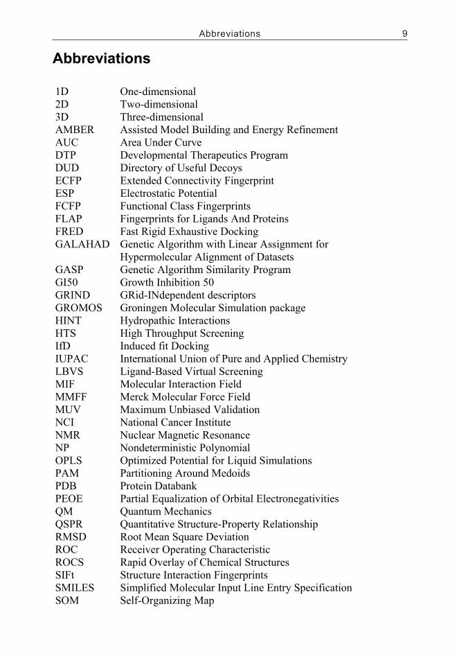
1D One-dimensional2D Two-dimensional3D Three-dimensionalAMBER Assisted Model Building and Energy RefinementAUC Area Under CurveDTP Developmental Therapeutics Program DUD Directory of Useful DecoysECFP Extended Connectivity FingerprintESP Electrostatic PotentialFCFP Functional Class FingerprintsFLAP Fingerprints for Ligands And ProteinsFRED Fast Rigid Exhaustive DockingGALAHAD Genetic Algorithm with Linear Assignment for
Hypermolecular Alignment of DatasetsGASP Genetic Algorithm Similarity ProgramGI50 Growth Inhibition 50GRIND GRid-INdependent descriptorsGROMOS Groningen Molecular Simulation packageHINT Hydropathic InteractionsHTS High Throughput ScreeningIfD Induced fit DockingIUPAC International Union of Pure and Applied ChemistryLBVS Ligand-Based Virtual ScreeningMIF Molecular Interaction FieldMMFF Merck Molecular Force FieldMUV Maximum Unbiased ValidationNCI National Cancer InstituteNMR Nuclear Magnetic ResonanceNP Nondeterministic PolynomialOPLS Optimized Potential for Liquid SimulationsPAM Partitioning Around Medoids PDB Protein DatabankPEOE Partial Equalization of Orbital ElectronegativitiesQM Quantum MechanicsQSPR Quantitative Structure-Property RelationshipRMSD Root Mean Square DeviationROC Receiver Operating CharacteristicROCS Rapid Overlay of Chemical StructuresSIFt Structure Interaction FingerprintsSMILES Simplified Molecular Input Line Entry SpecificationSOM Self-Organizing Map
Abbreviations 9
4.5.1 Enrichment of actives (I, II)..............................................................674.5.2 Scaffold hopping performance (III)..................................................67
4.6 Molecular scaffolds (III)..........................................................................684.7 Scaffold hopping analysis........................................................................68
4.7.1 Identification of scaffold hops (I)......................................................684.7.2 Scaffold hopping heatmaps (III)........................................................68
4.8 Similarity and group fusion......................................................................694.8.1 Similarity fusion (I, II)......................................................................694.8.2 Group fusion (II)...............................................................................70
4.9 Activity cliff analysis (II).........................................................................715 Results and discussion.....................................................................................72
5.1 Relationship between chemical and biological similarity (I)...................725.1.1 Single methods..................................................................................725.1.2 Combinations of methods..................................................................72
5.2 The enrichment of actives in the MUV dataset (II)..................................755.2.1 Non-overlapping binding poses.........................................................755.2.2 False negatives..................................................................................755.2.3 Activity cliffs.....................................................................................76
5.3 The effect of data fusion on the enrichment of actives............................765.3.1 Similarity fusion (I, II)......................................................................765.3.2 Group fusion (II)...............................................................................79
5.4 Scaffold hopping......................................................................................795.4.1 Example pairs (I)...............................................................................795.4.2 Scaffold heatmaps (III)......................................................................80
6 Conclusions.....................................................................................................837 Acknowledgements.........................................................................................848 References.......................................................................................................86Original publications I-III..................................................................................99
Abbreviations
1D One-dimensional2D Two-dimensional3D Three-dimensionalAMBER Assisted Model Building and Energy RefinementAUC Area Under CurveDTP Developmental Therapeutics Program DUD Directory of Useful DecoysECFP Extended Connectivity FingerprintESP Electrostatic PotentialFCFP Functional Class FingerprintsFLAP Fingerprints for Ligands And ProteinsFRED Fast Rigid Exhaustive DockingGALAHAD Genetic Algorithm with Linear Assignment for
Hypermolecular Alignment of DatasetsGASP Genetic Algorithm Similarity ProgramGI50 Growth Inhibition 50GRIND GRid-INdependent descriptorsGROMOS Groningen Molecular Simulation packageHINT Hydropathic InteractionsHTS High Throughput ScreeningIfD Induced fit DockingIUPAC International Union of Pure and Applied ChemistryLBVS Ligand-Based Virtual ScreeningMIF Molecular Interaction FieldMMFF Merck Molecular Force FieldMUV Maximum Unbiased ValidationNCI National Cancer InstituteNMR Nuclear Magnetic ResonanceNP Nondeterministic PolynomialOPLS Optimized Potential for Liquid SimulationsPAM Partitioning Around Medoids PDB Protein DatabankPEOE Partial Equalization of Orbital ElectronegativitiesQM Quantum MechanicsQSPR Quantitative Structure-Property RelationshipRMSD Root Mean Square DeviationROC Receiver Operating CharacteristicROCS Rapid Overlay of Chemical StructuresSIFt Structure Interaction FingerprintsSMILES Simplified Molecular Input Line Entry SpecificationSOM Self-Organizing Map

10 Abbreviations
SQL Structured Query LanguageTSS Turbo Similarity SearchingVS Virtual ScreeningZINC Zinc Is Not Commercial
List of original publications
This thesis is based on the following original publications, which are referred in the text by the Roman numerals I-III. The original communications have been reproduced with the permission of the copyright holders. Unpublished data is also included.
1 Tiikkainen P, Poso A, Kallioniemi O. Comparison of structure fingerprint and molecular interaction field based methods in explaining biological similarity of small molecules in cell-based screens. J Comput Aided Mol Des. 2009. Apr; 23(4):227-239.
2 Tiikkainen P*, Markt P*, Wolber G, Kirchmair J, Distinto S, Poso A, Kallioniemi O. Critical Comparison of Virtual Screening Methods Against the MUV Dataset. J Chem Inf Model. 2009. Oct; 49(10):2168-2178..
3 Tiikkainen P, Kallioniemi O, Poso A. Visualization and quantification of scaffold hopping with Ligand-based virtual screening tools. Submitted.
* Equal contribution

List of original publications 11
SQL Structured Query LanguageTSS Turbo Similarity SearchingVS Virtual ScreeningZINC Zinc Is Not Commercial
List of original publications
This thesis is based on the following original publications, which are referred in the text by the Roman numerals I-III. The original communications have been reproduced with the permission of the copyright holders. Unpublished data is also included.
1 Tiikkainen P, Poso A, Kallioniemi O. Comparison of structure fingerprint and molecular interaction field based methods in explaining biological similarity of small molecules in cell-based screens. J Comput Aided Mol Des. 2009. Apr; 23(4):227-239.
2 Tiikkainen P*, Markt P*, Wolber G, Kirchmair J, Distinto S, Poso A, Kallioniemi O. Critical Comparison of Virtual Screening Methods Against the MUV Dataset. J Chem Inf Model. 2009. Oct; 49(10):2168-2178..
3 Tiikkainen P, Kallioniemi O, Poso A. Visualization and quantification of scaffold hopping with Ligand-based virtual screening tools. Submitted.
* Equal contribution

12 Introduction
1 Introduction
Drug development projects are famous for their duration which can be over ten years and the costs which can go close to a billion US dollars. Roughly the drug discovery and development process is divided in pre-clinical and clinical phases.
Pre-clinical research starts from the identification of one or more therapeutically significant drug targets whose activity one wants to modulate, be it with small molecules, peptides or anti-bodies. Next an assay is developed (if one doesn’t already exists) which is used to screen a collection of molecules or antibodies for their activities. Once the hit molecules have been identified they usually need to be modified to improve their affinity and selectivity to the target. At this point the molecules are called lead molecules. Within pre-clinical development animal testing is vital for assessing the activity of the lead molecule in a complete organism.
After the lead molecule has been found to be effective and safe in animal testing it can be taken for clinical testing in humans. This phase divides further in four sub-phases: Phase I, Phase II, Phase III and Phase IV. In the first of these, safety of the drug candidate is evaluated on healthy volunteers. Efficacy is evaluated on patients in the other three phases. The second phase involves only a few dozen patients while the third phase is a multi-center study with up to thousands of patients. In each phase the drug candidate is compared to a placebo drug or an established treatment for the disease. The candidate drug must be more efficient than the existing treatment in order to be given a marketing permission by an agency regulating drug sales. Phase IV trials are conducted for drugs which have already been given the marketing permission. The purpose at this stage is to provide more information on the safety of the target using larger patient populations and for longer time periods than possible in the earlier phases. Additionally, interactions with other drugs can be studied in Phase IV.
Computer modeling is an essential component in modern pre-clinical drug discovery and development. Instead of testing each compound in a large compound library experimentally by using high-throughput screening (HTS), virtual screening tools can be used to rank molecules on their probability of binding to the target. This leads to considerable savings in personnel and material costs as only a small number of molecules of the complete library need to be tested experimentally.
Virtual screening tools are traditionally divided into structure-based and ligand-based methods. The former methods require a three-dimensional structure of
the target protein. Usually the structure is experimentally determined using either X-ray crystallography or Nuclear Magnetic Resonance (NMR) spectroscopy. Another option is to build a homology model using an experimentally determined structure of a related protein as a template. All structure-based virtual screening tools attempts to predict the shape and the electrostatic complementarity of the small molecule with the binding site of the protein. The most common way to perform this is docking where a rigid or flexible three-dimensional conformation of a molecule is fitted into the binding site and this so-called binding pose is scored. Another approach is to manually define a set of interactions required for binding and to only accept those molecules that fulfill most or all of these requirements.
In this thesis I have studied ligand-based virtual screening tools. In the first publication I related the chemical similarity scores for a set of molecules to the similarity of their cytotoxicity profiles. This led to important findings on the advantages and deficiencies of different tools. The results also allowed me to estimate the biological similarity of a molecule pair given their chemical similarity values calculated with one or more tools. Combination of different tools led to synergy and improved retrieval of actives in a retrospective screen. In the second paper, the capability of five similarity search tools and two pharmacophore elucidators were assessed in a retrospective virtual screen against the Maximum Unbiased Validation (MUV) benchmark set. The dataset contains known active molecules and simple property matched inactive (decoy) molecules divided into 17 target classes. Performance of the tools was found to be disappointing with most target classes. Three potential reasons were identified: false negatives, non-overlapping binding modes and activity cliffs. The first and second reason is due to the data set used and should be taken in to account when designing future benchmark sets. The third reason is more difficult to resolve as long as only chemical information of the two molecules being compared is available. In the third paper I designed and evaluated an approach for visualizing and quantifying the scaffold hopping capability of ligand-based virtual screening tools. Two 3D overlay tools (BRUTUS and EON) were found to perform best while also the third tool evaluated (ROCS) performed well with certain ligand sets.

Introduction 13
1 Introduction
Drug development projects are famous for their duration which can be over ten years and the costs which can go close to a billion US dollars. Roughly the drug discovery and development process is divided in pre-clinical and clinical phases.
Pre-clinical research starts from the identification of one or more therapeutically significant drug targets whose activity one wants to modulate, be it with small molecules, peptides or anti-bodies. Next an assay is developed (if one doesn’t already exists) which is used to screen a collection of molecules or antibodies for their activities. Once the hit molecules have been identified they usually need to be modified to improve their affinity and selectivity to the target. At this point the molecules are called lead molecules. Within pre-clinical development animal testing is vital for assessing the activity of the lead molecule in a complete organism.
After the lead molecule has been found to be effective and safe in animal testing it can be taken for clinical testing in humans. This phase divides further in four sub-phases: Phase I, Phase II, Phase III and Phase IV. In the first of these, safety of the drug candidate is evaluated on healthy volunteers. Efficacy is evaluated on patients in the other three phases. The second phase involves only a few dozen patients while the third phase is a multi-center study with up to thousands of patients. In each phase the drug candidate is compared to a placebo drug or an established treatment for the disease. The candidate drug must be more efficient than the existing treatment in order to be given a marketing permission by an agency regulating drug sales. Phase IV trials are conducted for drugs which have already been given the marketing permission. The purpose at this stage is to provide more information on the safety of the target using larger patient populations and for longer time periods than possible in the earlier phases. Additionally, interactions with other drugs can be studied in Phase IV.
Computer modeling is an essential component in modern pre-clinical drug discovery and development. Instead of testing each compound in a large compound library experimentally by using high-throughput screening (HTS), virtual screening tools can be used to rank molecules on their probability of binding to the target. This leads to considerable savings in personnel and material costs as only a small number of molecules of the complete library need to be tested experimentally.
Virtual screening tools are traditionally divided into structure-based and ligand-based methods. The former methods require a three-dimensional structure of
the target protein. Usually the structure is experimentally determined using either X-ray crystallography or Nuclear Magnetic Resonance (NMR) spectroscopy. Another option is to build a homology model using an experimentally determined structure of a related protein as a template. All structure-based virtual screening tools attempts to predict the shape and the electrostatic complementarity of the small molecule with the binding site of the protein. The most common way to perform this is docking where a rigid or flexible three-dimensional conformation of a molecule is fitted into the binding site and this so-called binding pose is scored. Another approach is to manually define a set of interactions required for binding and to only accept those molecules that fulfill most or all of these requirements.
In this thesis I have studied ligand-based virtual screening tools. In the first publication I related the chemical similarity scores for a set of molecules to the similarity of their cytotoxicity profiles. This led to important findings on the advantages and deficiencies of different tools. The results also allowed me to estimate the biological similarity of a molecule pair given their chemical similarity values calculated with one or more tools. Combination of different tools led to synergy and improved retrieval of actives in a retrospective screen. In the second paper, the capability of five similarity search tools and two pharmacophore elucidators were assessed in a retrospective virtual screen against the Maximum Unbiased Validation (MUV) benchmark set. The dataset contains known active molecules and simple property matched inactive (decoy) molecules divided into 17 target classes. Performance of the tools was found to be disappointing with most target classes. Three potential reasons were identified: false negatives, non-overlapping binding modes and activity cliffs. The first and second reason is due to the data set used and should be taken in to account when designing future benchmark sets. The third reason is more difficult to resolve as long as only chemical information of the two molecules being compared is available. In the third paper I designed and evaluated an approach for visualizing and quantifying the scaffold hopping capability of ligand-based virtual screening tools. Two 3D overlay tools (BRUTUS and EON) were found to perform best while also the third tool evaluated (ROCS) performed well with certain ligand sets.

14 Review of literature
2 Review of literature
2.1 Modeling of small molecules
2.1.1 Representation of molecules
When working with small molecule it is important that they are properly. This includes assigning a proper protonation and tautomeric states for the molecule. Many bioactive drugs come as combinations of different stereoisomers (i.e. racemic mixtures) and not all isomers are necessarily active. Choosing the correct stereoisomer for modeling can have a significant effect on the end result. These issues are described more in detail in the following chapters.
2.1.1.1 Atom and bond types
Organic small molecules consist of only a small subset of all elements in nature – most notably carbon, nitrogen, oxygen, phosphate, sulfur, hydrogen and halogens. However, in chemoinformatics and molecular modeling it is usually not enough to designate an atom by its element. The environment of an atom also dictates its chemical properties. Therefore elements are divided into atom types as function of their environment. Figure 1 illustrates different Sybyl atom types [1, 2] for oxygen.
Atom type is used to model interactions of the atom with its environment. For example, a hydrogen bond with an ether oxygen (O.3 atom in Figure 1) as acceptor is weaker than a carbonyl oxygen (O.2 atom in Figure 1). Therefore differentiating these two types of oxygen is important for reliable calculations. The atom types are assigned by following a set of hierarchical rules. For instance, Tripos atom types can be derived as described in ref [3].
Bond types are closely related to atom types. They also have effect on the calculations, for example double bonds are shorter and more electronegative than single bonds. There are five defined Tripos bond types: single, double, triple, aromatic and amide. The amide bond is used exclusively between the nitrogen and the carbon in an amide group.
In addition to the Tripos atom types given as an example above, other atom typing schemes include for example the IDATM atom types [4] implemented in the structure analysis tool Chimera [5] or those implemented in the freely available docking tool AutoDock [6].
Figure 1. Three oxygen atom types. Carbonyl (double bonded) oxygens have type O.2, and
the ether oxygen has type O.3. Oxygens in a carboxyl group have a special atom type
O.co2 to account for the delocalized electron shared by the oxygens and thus
differentiating them from carbonyl oxygens.
2.1.1.2 Stereoisomerism
A central theme in organic chemistry is stereoisomerism. Two stereoisomers have the same molecular formula and the same atom connectivity. They differ only in the three dimensional orientations of their atoms in such a way that they cannot be overlaid in space. Such molecules are said to be chiral.
Many molecules found in nature can only be found as one stereoisomer. Also a large proportion of drugs are chiral and often only one of the isomers is therapeutically active while the other isomers are either inactive or even toxic. Examples of drugs that have stereospecific activity include quinidine [7] and ethambutol [8]. Administrating the safe isomer to the patient is not necessarily enough to circumvent the problem as the body is sometimes able to interconvert one isomer to another. For example (R)-thalidomide is effective against morning sickness while (S)-thalidomide is teratogenic. The apparent solution to avoid teratogenicity would therefore be to administer only the safe (R)-isomer. Unfortunately this strategy would fail as the body can convert the safe isomer into the teratogenic one [9].
One of the most common forms of stereoisomerism results from a carbon atom having four different substituents attached to it (a chiral center). These groups can be attached in two ways leading to two non-superimposable isomers called enantiomers [Figure 2]. A popular analogy is the left and the right hand that cannot be overlaid.

Review of literature 15
2 Review of literature
2.1 Modeling of small molecules
2.1.1 Representation of molecules
When working with small molecule it is important that they are properly. This includes assigning a proper protonation and tautomeric states for the molecule. Many bioactive drugs come as combinations of different stereoisomers (i.e. racemic mixtures) and not all isomers are necessarily active. Choosing the correct stereoisomer for modeling can have a significant effect on the end result. These issues are described more in detail in the following chapters.
2.1.1.1 Atom and bond types
Organic small molecules consist of only a small subset of all elements in nature – most notably carbon, nitrogen, oxygen, phosphate, sulfur, hydrogen and halogens. However, in chemoinformatics and molecular modeling it is usually not enough to designate an atom by its element. The environment of an atom also dictates its chemical properties. Therefore elements are divided into atom types as function of their environment. Figure 1 illustrates different Sybyl atom types [1, 2] for oxygen.
Atom type is used to model interactions of the atom with its environment. For example, a hydrogen bond with an ether oxygen (O.3 atom in Figure 1) as acceptor is weaker than a carbonyl oxygen (O.2 atom in Figure 1). Therefore differentiating these two types of oxygen is important for reliable calculations. The atom types are assigned by following a set of hierarchical rules. For instance, Tripos atom types can be derived as described in ref [3].
Bond types are closely related to atom types. They also have effect on the calculations, for example double bonds are shorter and more electronegative than single bonds. There are five defined Tripos bond types: single, double, triple, aromatic and amide. The amide bond is used exclusively between the nitrogen and the carbon in an amide group.
In addition to the Tripos atom types given as an example above, other atom typing schemes include for example the IDATM atom types [4] implemented in the structure analysis tool Chimera [5] or those implemented in the freely available docking tool AutoDock [6].
Figure 1. Three oxygen atom types. Carbonyl (double bonded) oxygens have type O.2, and
the ether oxygen has type O.3. Oxygens in a carboxyl group have a special atom type
O.co2 to account for the delocalized electron shared by the oxygens and thus
differentiating them from carbonyl oxygens.
2.1.1.2 Stereoisomerism
A central theme in organic chemistry is stereoisomerism. Two stereoisomers have the same molecular formula and the same atom connectivity. They differ only in the three dimensional orientations of their atoms in such a way that they cannot be overlaid in space. Such molecules are said to be chiral.
Many molecules found in nature can only be found as one stereoisomer. Also a large proportion of drugs are chiral and often only one of the isomers is therapeutically active while the other isomers are either inactive or even toxic. Examples of drugs that have stereospecific activity include quinidine [7] and ethambutol [8]. Administrating the safe isomer to the patient is not necessarily enough to circumvent the problem as the body is sometimes able to interconvert one isomer to another. For example (R)-thalidomide is effective against morning sickness while (S)-thalidomide is teratogenic. The apparent solution to avoid teratogenicity would therefore be to administer only the safe (R)-isomer. Unfortunately this strategy would fail as the body can convert the safe isomer into the teratogenic one [9].
One of the most common forms of stereoisomerism results from a carbon atom having four different substituents attached to it (a chiral center). These groups can be attached in two ways leading to two non-superimposable isomers called enantiomers [Figure 2]. A popular analogy is the left and the right hand that cannot be overlaid.

16 Review of literature
Figure 2. Both enantiomers of a molecule with one chiral carbon atom (arrow).
Stereoisomerism can also arise if the molecule has a carbon-carbon double bond with different substituents on both sides of the bond [Figure 3]. As rotation of the double bond is restricted, we have two ways to arrange the substituents in a way the two isomers cannot be overlaid.
Figure 3. Different substituents on both sides of the double bond make it impossible to
overlay the isomers. The molecule to the left is called the (E)-isomer while the one to the
right is the (Z)-isomer.
Two isomers can have different physiological and biological properties and should therefore be treated separately. When performing 3D virtual screening it is important to use the relevant stereoisomer of the molecule. In combinatorial chemistry libraries, the compounds usually exists as racemic mixtures (i.e. contain more than one stereoisomer). A 3D model for each possible stereoisomer should be generated and handled as if they were separate molecules. Sometimes a 3D model of a stereoisomer is not possible due to steric clashes and such isomers are therefore excluded from further analysis at the 3D conformer generation step. This can happen for example when there are two very bulky substituents on the same side of a double bond (Z-isomer) and therefore only the (E)-isomer could be sterically possible. In the analysis step of virtual screening, results for different stereoisomer of a molecule can be merged, e.g. the stereoisomer with the highest score could be chosen to represent all isomers of the molecule.
2.1.1.3 Ionic state (pKa)
The ionization state of weak acids and bases dictate several properties of a small molecule. In order to reach its target, it is important that the molecule is in its neutral form when crossing a hydrophobic obstacle such as a cell membrane. When interacting with the target protein, formation of a hydrogen bond can depend on the proper ionization state of the ligand’s functional group participating in the interaction [10].
Degree of (de-)protonation of an ionizable group is quantified with the equilibrium constant Ka given in Equation 1 where [A-] equals the concentration of deprotonated species, [H+] is the concentration of unbound protons and [HA] is the concentration of the protonated species
Equation 1
[ ][ ][ ]HA
HAKa
+−
=
The linkage between the pH and the negative logarithm of the equilibrium constant (pKa) is given by the Henderson-Hasselbach equation [Equation 2]. The pKa value assigned to a compound is the pH value where the de-protonated and the protonated species can be found in equal concentrations (in Equation 2 the logarithm term becomes zero as log 1 = 0).
Equation 2
[ ][ ]HA
ApKpH a
−
+= 10log
For molecules with a single protonation site, the pKa value can be determined by titrating the solution with a strong base or acid and plotting the ratio of the two ionic states as function of pH. For molecules with more protonation sites, the situation becomes more complex as the number of possible ionic species increases.
Determining the dominant protonation state of a small molecule at a given pH is an important application of computational chemistry. A wide variety of methods has been developed to tackle the task. Most of them rely on training a model with molecules for which experimental pKa values are known. Also ab
initio methods have been used. These methods are based on fundamental physical properties and therefore do not require training sets of molecules.

Review of literature 17
Figure 2. Both enantiomers of a molecule with one chiral carbon atom (arrow).
Stereoisomerism can also arise if the molecule has a carbon-carbon double bond with different substituents on both sides of the bond [Figure 3]. As rotation of the double bond is restricted, we have two ways to arrange the substituents in a way the two isomers cannot be overlaid.
Figure 3. Different substituents on both sides of the double bond make it impossible to
overlay the isomers. The molecule to the left is called the (E)-isomer while the one to the
right is the (Z)-isomer.
Two isomers can have different physiological and biological properties and should therefore be treated separately. When performing 3D virtual screening it is important to use the relevant stereoisomer of the molecule. In combinatorial chemistry libraries, the compounds usually exists as racemic mixtures (i.e. contain more than one stereoisomer). A 3D model for each possible stereoisomer should be generated and handled as if they were separate molecules. Sometimes a 3D model of a stereoisomer is not possible due to steric clashes and such isomers are therefore excluded from further analysis at the 3D conformer generation step. This can happen for example when there are two very bulky substituents on the same side of a double bond (Z-isomer) and therefore only the (E)-isomer could be sterically possible. In the analysis step of virtual screening, results for different stereoisomer of a molecule can be merged, e.g. the stereoisomer with the highest score could be chosen to represent all isomers of the molecule.
2.1.1.3 Ionic state (pKa)
The ionization state of weak acids and bases dictate several properties of a small molecule. In order to reach its target, it is important that the molecule is in its neutral form when crossing a hydrophobic obstacle such as a cell membrane. When interacting with the target protein, formation of a hydrogen bond can depend on the proper ionization state of the ligand’s functional group participating in the interaction [10].
Degree of (de-)protonation of an ionizable group is quantified with the equilibrium constant Ka given in Equation 1 where [A-] equals the concentration of deprotonated species, [H+] is the concentration of unbound protons and [HA] is the concentration of the protonated species
Equation 1
[ ][ ][ ]HA
HAKa
+−
=
The linkage between the pH and the negative logarithm of the equilibrium constant (pKa) is given by the Henderson-Hasselbach equation [Equation 2]. The pKa value assigned to a compound is the pH value where the de-protonated and the protonated species can be found in equal concentrations (in Equation 2 the logarithm term becomes zero as log 1 = 0).
Equation 2
[ ][ ]HA
ApKpH a
−
+= 10log
For molecules with a single protonation site, the pKa value can be determined by titrating the solution with a strong base or acid and plotting the ratio of the two ionic states as function of pH. For molecules with more protonation sites, the situation becomes more complex as the number of possible ionic species increases.
Determining the dominant protonation state of a small molecule at a given pH is an important application of computational chemistry. A wide variety of methods has been developed to tackle the task. Most of them rely on training a model with molecules for which experimental pKa values are known. Also ab
initio methods have been used. These methods are based on fundamental physical properties and therefore do not require training sets of molecules.

18 Review of literature
The most popular approach is to train a QSPR (Quantitative Structure-Property Relationship) model using a given set of molecular descriptors [11]. Typically a single model is trained for a certain chemical group. This naturally restricts the applicability of the model. In practice, a set of models are generated each specialized to predict the pKa value for a given functional group.
More recently topological look-up methods have been applied where the immediate atom neighborhood of the ionizable site is used to predict the correct protonation state [12-14]. The neighborhood is defined with circular fingerprints that encode information of atoms at each distance step from the ionizable atom up to a given maximum distance.
Molecular interaction fields (more on these below) were used by Milletti et al. [15] for pKa prediction. The training set consisted of 466 semi-rigid fragments with known pKa values. For each fragment, an ionizable or nonionizable reference group/atom was picked whose minimum interaction potential to 10 probes was measured with the GRID software (see section on the program below). Different fragments were used to control the effect the surrounding atoms have on the pKa constant of the reference group. The interaction value for each probe was finally binned. 33 separate predictive models were built (one for five-membered heterocycles, for example) for predicting the pKa value as a function of the binned interaction energy of an ionizable atom and its surroundings. Given a novel molecule, the ionizable group and its surroundings is mapped to one of the 33 models based on the MIF interaction bins. The approach was evaluated with an external dataset of 28 novel compounds and good correspondence with the experimental and predicted pKa values was observed.
The advantage of trained models described so far is their speed. However, applicability of a given model is restricted and will most probably fail when a structurally different molecule is presented. Quantum Mechanical (QM) methods offer an alternative as they do not require a training set for making the prediction [16]. These methods provide accurate predictions but are computationally very expensive rendering them inapplicable for predicting pKa values for large databases of molecules.
2.1.2 1D descriptors
The simplest descriptors or properties of small molecules are the so-called 1D descriptors which include scalars for molecular weight, atom count, charge and number of rotatable bonds. These are familiar even to people with limited knowledge of chemistry. Most of these are straightforward to calculate, for instance molecular weight is just the sum of weights of the atoms in the
molecule. Despite their simplicity – or perhaps just because of it – 1D properties are widely used to describe things like general characteristics of small molecule libraries or to predict the solubility and permeability of small molecules [17].
In the following chapters, some less trivial molecular scalar properties are described.
2.1.2.1 log P and log D
One of the single most important properties of a small molecule is its solubility in water which influences both its pharmacokinetic and pharmacodynamic properties.
If a molecule is overly soluble it does not pass the intestinal lipid epithelium easily and it therefore becomes difficult to administer it orally.– a major factor for practical use of a drug. In contrast, a molecule with poor solubility readily desolves into the epithelium but not in the cytosol meaning it is not able to bind any intracellular targets [18]. One strategy to improve intestinal cell wall permeability is to use a pro-drug, i.e. a more lipophilic analog of the actual drug which is metabolized into the active form in vivo.
If the molecule is able to reach its intended target, solubility still plays an important role in the binding process. The hydrophobic effect is very important in binding but again the molecule must strike a balance between hydrophobicity and solubility [19, 20]. Molecules that are overly hydrophobic tend to be less specific binders and are also metabolized more readily. Both factors are risk factors for toxic side effects. If binding to the target requires specific electrostatic or hydrogen bonding interactions, being too hydrophobic (i.e. lack of complementary hydrogen bonding partners for example) is naturally a drawback. In the other end of the hydrophobicity spectrum, molecules overly hydrophilic (soluble) might not be able to leave the water phase (de-solve) and bind to the target.
The most common way to describe the lipophilicity of a molecule is with the partition coefficient which is the logarithm of the ratio of concentrations of the molecule in octanol (or some other hydrophobic solvent) and water [21]. There are two kinds of partition coefficients, log P and log D. When determining the former the pH of the water phase is set so that majority of the compound is non-ionized. The latter property gives the partition coefficient of the molecule as a function of pH, i.e. the molecule can also be ionized. Usually log D is measured at the physiological pH of 7.4. The majority of drug molecules are ionizable meaning that log D should be used in describing them.
Review of literature 19
The most popular approach is to train a QSPR (Quantitative Structure-Property Relationship) model using a given set of molecular descriptors [11]. Typically a single model is trained for a certain chemical group. This naturally restricts the applicability of the model. In practice, a set of models are generated each specialized to predict the pKa value for a given functional group.
More recently topological look-up methods have been applied where the immediate atom neighborhood of the ionizable site is used to predict the correct protonation state [12-14]. The neighborhood is defined with circular fingerprints that encode information of atoms at each distance step from the ionizable atom up to a given maximum distance.
Molecular interaction fields (more on these below) were used by Milletti et al. [15] for pKa prediction. The training set consisted of 466 semi-rigid fragments with known pKa values. For each fragment, an ionizable or nonionizable reference group/atom was picked whose minimum interaction potential to 10 probes was measured with the GRID software (see section on the program below). Different fragments were used to control the effect the surrounding atoms have on the pKa constant of the reference group. The interaction value for each probe was finally binned. 33 separate predictive models were built (one for five-membered heterocycles, for example) for predicting the pKa value as a function of the binned interaction energy of an ionizable atom and its surroundings. Given a novel molecule, the ionizable group and its surroundings is mapped to one of the 33 models based on the MIF interaction bins. The approach was evaluated with an external dataset of 28 novel compounds and good correspondence with the experimental and predicted pKa values was observed.
The advantage of trained models described so far is their speed. However, applicability of a given model is restricted and will most probably fail when a structurally different molecule is presented. Quantum Mechanical (QM) methods offer an alternative as they do not require a training set for making the prediction [16]. These methods provide accurate predictions but are computationally very expensive rendering them inapplicable for predicting pKa values for large databases of molecules.
2.1.2 1D descriptors
The simplest descriptors or properties of small molecules are the so-called 1D descriptors which include scalars for molecular weight, atom count, charge and number of rotatable bonds. These are familiar even to people with limited knowledge of chemistry. Most of these are straightforward to calculate, for instance molecular weight is just the sum of weights of the atoms in the
molecule. Despite their simplicity – or perhaps just because of it – 1D properties are widely used to describe things like general characteristics of small molecule libraries or to predict the solubility and permeability of small molecules [17].
In the following chapters, some less trivial molecular scalar properties are described.
2.1.2.1 log P and log D
One of the single most important properties of a small molecule is its solubility in water which influences both its pharmacokinetic and pharmacodynamic properties.
If a molecule is overly soluble it does not pass the intestinal lipid epithelium easily and it therefore becomes difficult to administer it orally.– a major factor for practical use of a drug. In contrast, a molecule with poor solubility readily desolves into the epithelium but not in the cytosol meaning it is not able to bind any intracellular targets [18]. One strategy to improve intestinal cell wall permeability is to use a pro-drug, i.e. a more lipophilic analog of the actual drug which is metabolized into the active form in vivo.
If the molecule is able to reach its intended target, solubility still plays an important role in the binding process. The hydrophobic effect is very important in binding but again the molecule must strike a balance between hydrophobicity and solubility [19, 20]. Molecules that are overly hydrophobic tend to be less specific binders and are also metabolized more readily. Both factors are risk factors for toxic side effects. If binding to the target requires specific electrostatic or hydrogen bonding interactions, being too hydrophobic (i.e. lack of complementary hydrogen bonding partners for example) is naturally a drawback. In the other end of the hydrophobicity spectrum, molecules overly hydrophilic (soluble) might not be able to leave the water phase (de-solve) and bind to the target.
The most common way to describe the lipophilicity of a molecule is with the partition coefficient which is the logarithm of the ratio of concentrations of the molecule in octanol (or some other hydrophobic solvent) and water [21]. There are two kinds of partition coefficients, log P and log D. When determining the former the pH of the water phase is set so that majority of the compound is non-ionized. The latter property gives the partition coefficient of the molecule as a function of pH, i.e. the molecule can also be ionized. Usually log D is measured at the physiological pH of 7.4. The majority of drug molecules are ionizable meaning that log D should be used in describing them.

20 Review of literature
Experimental determination of the partition coefficient for large compound libraries is unfeasible. Several computational methods have therefore been developed for predicting the coefficient. The most popular are regression models trained using molecules with experimentally determined partition coefficients. In the software MLogP [22], each element frequently found in drug molecules is divided into a number of atom types depending on its neighboring atoms. Each atom type is assigned a hydrophobicity value. When the partition coefficient is calculated for a molecule, hydrophobicity values of its atoms are simply added up. These methods give only rough estimates but are fast and universal as the most commonly occurring atom types are parameterized. Another way to build a log P estimator is to use molecular fragments of known lipophilicity as a training material. This is the approach taken in the ClogP software [23] which breaks the molecule into fragments which are further divided based on their bonding environment. The fragment values are added up and corrections are made if they occur close to each other.
More advanced methods to predict the partition coefficient are possible with machine learning techniques. These include work done with neural networks [24] and support vector machines [25]. Their results are superior compared to the simple regression models but with the caveat that the compounds predicted must resemble the training set molecules.
2.1.2.2 Point charges
Distribution of electrons around positively charged nuclei of a molecule can be considered as a cloud represented mathematically as a probability function. This information can be obtained either experimentally by X-ray crystallography or computationally by using quantum mechanics methods. Although accurate, the latter approach is computationally too expensive in order to be practical in virtual screening. The charge distribution is simplified by assigning a so-called partial or point charge located in the center of each atom in a molecule.
The most common approach to calculate point charges is based on the Partial Equalization of Orbital Electronegativities (PEOE) method originally introduced by Gasteiger and Marsili [26]. This is an iterative process where each atom is first given an initial point charge (its formal charge). Next the point charge of each atom is altered based on the electronegativity of its neighbors. This is done to simulate movement of electrons from less electronegative atoms towards more electronegative ones. This step is repeated a few times until convergence is reached. This algorithm takes only sigma bonds into account. The more advanced Gasteiger-Hückel approach takes also
π-bond systems into account [27]. Charges of atoms that are part of a π-system are considered to be de-localized across the whole system. First the π -component of the point charge is calculated using Hückel’s approach [28]. After this the Gasteiger charge calculation is done for the σ component.
The topological methods described above are computationally inexpensive and fairly accurate for atoms that have been parameterized. This explains the popularity of these methods. Quantum mechanical functions take the three-dimensional structure of the molecule into account for point charge determinations and give more accurate results. However, calculation and analysis of the wave function describing electron distributions requires lots of computer power. Semiempirical methods such as the electrostatic potential (ESP) fit method are widely used when more accurate charge models are required [29]. The point charges are fitted in the atoms by least-squares fitting from a charge density calculated quantum mechanically for a set of points surrounding the molecule. It is important to remember that there is no experimental method to determine point charges and therefore it is impossible to evaluate if an individual point charge is “correct”.
2.1.3 3D conformations
Representing molecules only in two dimensions is naturally a simplification of the real world where everything takes place in three dimensions. Therefore molecular modeling tools handling 3D models of molecules are important. Having a three-dimensional model of a small molecule is absolutely vital in applications such as docking and molecular superposition which are discussed later. In the following chapter, methods which transform a two-dimensional structure into a three-dimensional conformation are introduced. Also tools that explore the conformational space to generate an ensemble of conformers are described.
2.1.3.1 Converting 2D structures to 3D
Automatic 3D model builders - that convert a 2D structure into a 3D model automatically without human intervention – can be divided into fragment and rule- and data-based tools [30]. Often a single tool cannot be strictly classified to belong to only one class since they can combine techniques from both classes. Numerical methods which apply quantum and/or molecular mechanics calculations to derive a conformer usually require a reasonable starting conformation and thus cannot be considered as automatic methods. These are discussed in more detail in the “Conformational analysis” section.

Review of literature 21
Experimental determination of the partition coefficient for large compound libraries is unfeasible. Several computational methods have therefore been developed for predicting the coefficient. The most popular are regression models trained using molecules with experimentally determined partition coefficients. In the software MLogP [22], each element frequently found in drug molecules is divided into a number of atom types depending on its neighboring atoms. Each atom type is assigned a hydrophobicity value. When the partition coefficient is calculated for a molecule, hydrophobicity values of its atoms are simply added up. These methods give only rough estimates but are fast and universal as the most commonly occurring atom types are parameterized. Another way to build a log P estimator is to use molecular fragments of known lipophilicity as a training material. This is the approach taken in the ClogP software [23] which breaks the molecule into fragments which are further divided based on their bonding environment. The fragment values are added up and corrections are made if they occur close to each other.
More advanced methods to predict the partition coefficient are possible with machine learning techniques. These include work done with neural networks [24] and support vector machines [25]. Their results are superior compared to the simple regression models but with the caveat that the compounds predicted must resemble the training set molecules.
2.1.2.2 Point charges
Distribution of electrons around positively charged nuclei of a molecule can be considered as a cloud represented mathematically as a probability function. This information can be obtained either experimentally by X-ray crystallography or computationally by using quantum mechanics methods. Although accurate, the latter approach is computationally too expensive in order to be practical in virtual screening. The charge distribution is simplified by assigning a so-called partial or point charge located in the center of each atom in a molecule.
The most common approach to calculate point charges is based on the Partial Equalization of Orbital Electronegativities (PEOE) method originally introduced by Gasteiger and Marsili [26]. This is an iterative process where each atom is first given an initial point charge (its formal charge). Next the point charge of each atom is altered based on the electronegativity of its neighbors. This is done to simulate movement of electrons from less electronegative atoms towards more electronegative ones. This step is repeated a few times until convergence is reached. This algorithm takes only sigma bonds into account. The more advanced Gasteiger-Hückel approach takes also
π-bond systems into account [27]. Charges of atoms that are part of a π-system are considered to be de-localized across the whole system. First the π -component of the point charge is calculated using Hückel’s approach [28]. After this the Gasteiger charge calculation is done for the σ component.
The topological methods described above are computationally inexpensive and fairly accurate for atoms that have been parameterized. This explains the popularity of these methods. Quantum mechanical functions take the three-dimensional structure of the molecule into account for point charge determinations and give more accurate results. However, calculation and analysis of the wave function describing electron distributions requires lots of computer power. Semiempirical methods such as the electrostatic potential (ESP) fit method are widely used when more accurate charge models are required [29]. The point charges are fitted in the atoms by least-squares fitting from a charge density calculated quantum mechanically for a set of points surrounding the molecule. It is important to remember that there is no experimental method to determine point charges and therefore it is impossible to evaluate if an individual point charge is “correct”.
2.1.3 3D conformations
Representing molecules only in two dimensions is naturally a simplification of the real world where everything takes place in three dimensions. Therefore molecular modeling tools handling 3D models of molecules are important. Having a three-dimensional model of a small molecule is absolutely vital in applications such as docking and molecular superposition which are discussed later. In the following chapter, methods which transform a two-dimensional structure into a three-dimensional conformation are introduced. Also tools that explore the conformational space to generate an ensemble of conformers are described.
2.1.3.1 Converting 2D structures to 3D
Automatic 3D model builders - that convert a 2D structure into a 3D model automatically without human intervention – can be divided into fragment and rule- and data-based tools [30]. Often a single tool cannot be strictly classified to belong to only one class since they can combine techniques from both classes. Numerical methods which apply quantum and/or molecular mechanics calculations to derive a conformer usually require a reasonable starting conformation and thus cannot be considered as automatic methods. These are discussed in more detail in the “Conformational analysis” section.

22 Review of literature
Fragment-based model building methods first divide a molecule into (partially overlapping) fragments. Fragment conformers are then derived from a library containing pre-defined and optimized conformations derived experimentally and/or from force field calculations. Then the molecule is merged for an initial 3D model. Any steric clashes between atoms from different fragments still need to be resolved by turning torsion angles. COBRA [31, 32] is an example of a tool that applies fragmentation as part of its algorithm.
Rule- and data-based methods apply a set of pre-determined rules derived from experimental data when assigning critical parameters like bond lengths and bond angles. These parameters depend heavily on type and hybridization state of the directly connected atoms. Rings and acyclic chains are usually treated separately. As smaller rings (less than 10 heavy atoms) are rather rigid, a pre-determined low-energy conformer taken from a fragment library can be used. Acyclic chains allow a much larger conformational variation and iterating through all conformations would be inefficient. Therefore most methods represent acyclic chains in an extended conformation by assigning all bonds in the trans configuration unless a double bond in the cis configuration is given. This efficiently prevents any clashes between atoms not directly bonded. Examples of 3D generators in this category include CORINA [33] and CONCORD [34].
2.1.3.2 Conformational analysis
Molecules can adopt many different.. Each conformer corresponds to a distinct local minimum in the energy landscape. Figure 4 gives an example of a conformer energy landscape for a compound, tiotidine. Changes in conformation take place by changes in torsion angles while the bond lengths and angles remain practically constant.
An important application of conformational analysis is to find the so called bioactive conformer, i.e. the pose a small molecule adopts when binding to its macromolecular target [35]. There is no straightforward rule to decide if a given conformer of a ligand is the bioactive conformation against a given target. Therefore ensembles of low-energy conformations must be sampled assuming that the bioactive conformer is among these. Knowledge of the binding pose is invaluable when developing other molecules with better properties that target the same macromolecule [36]. In absence of experimental information such as a high resolution X-ray crystal structure, computational tools are needed for picking the correct conformer from several energetically accessible ones [37]. An additional confounding factor is that a drug molecule can have more than one bioactive conformer if it binds to several targets [38].
In the following chapters five main approaches to conformer analysis are presented each of which has its advantages and deficiencies.
2.1.3.2.1 Systematic search
The most intuitive approach to generate an ensemble of conformers is the systematic search [39]. From a starting position, each torsion angle of the molecule is systematically altered in turn by a certain step size (e.g. 30 degrees). This strategy generates a lot of conformers if the molecule is flexible, i.e. it has several rotatable bonds. The number of conformations grows exponentially with the number of rotatable bonds (n in Equation 3).
Equation 3
( ) nsizestepcountConformer _/360_ =
To restrict the number of conformers taken for the final analysis, a number of filtering steps should be applied. The first filter is the so called “bump check” where conformers with atoms not directly connected and having overlapping van der Waals radii are removed. This step is done before calculating the energy for the conformer therefore saving precious computational resources.
After the bump check conformer energies are calculated with a force field such as the one in Equation 5. The second step is to exclude any conformer with a too large energy difference to the minimum energy conformer found. This energy window depends on the force field used and usually ranges from 5 to 15 kcal/mol. This window should not be too restrictive as the energy of the bioactive conformation can differ quite a bit from the global minimum [40-42].
After these two steps, the number of conformers can still be too large. Fortunately, it is still possible to reduce the number of conformers by clustering similar conformers into clusters and to choose one conformer to represent each cluster [43]. Figure 4b is an example of such clustering. In this case, the SOM clustering algorithm [44] was used to group similar conformers together. “Altitude” of a node on the map corresponds to the energy of the lowest energy conformer of the node. Picking a conformer from each low-energy node for further analysis would be an efficient strategy in this case.
The clear advantage of using systematic search is its completeness as each combination of torsion angles is explored. This is also the largest disadvantage of the method as this is computationally expensive and storing the results takes lots of hard disk space. Therefore it is only applicable for compounds with

Review of literature 23
Fragment-based model building methods first divide a molecule into (partially overlapping) fragments. Fragment conformers are then derived from a library containing pre-defined and optimized conformations derived experimentally and/or from force field calculations. Then the molecule is merged for an initial 3D model. Any steric clashes between atoms from different fragments still need to be resolved by turning torsion angles. COBRA [31, 32] is an example of a tool that applies fragmentation as part of its algorithm.
Rule- and data-based methods apply a set of pre-determined rules derived from experimental data when assigning critical parameters like bond lengths and bond angles. These parameters depend heavily on type and hybridization state of the directly connected atoms. Rings and acyclic chains are usually treated separately. As smaller rings (less than 10 heavy atoms) are rather rigid, a pre-determined low-energy conformer taken from a fragment library can be used. Acyclic chains allow a much larger conformational variation and iterating through all conformations would be inefficient. Therefore most methods represent acyclic chains in an extended conformation by assigning all bonds in the trans configuration unless a double bond in the cis configuration is given. This efficiently prevents any clashes between atoms not directly bonded. Examples of 3D generators in this category include CORINA [33] and CONCORD [34].
2.1.3.2 Conformational analysis
Molecules can adopt many different.. Each conformer corresponds to a distinct local minimum in the energy landscape. Figure 4 gives an example of a conformer energy landscape for a compound, tiotidine. Changes in conformation take place by changes in torsion angles while the bond lengths and angles remain practically constant.
An important application of conformational analysis is to find the so called bioactive conformer, i.e. the pose a small molecule adopts when binding to its macromolecular target [35]. There is no straightforward rule to decide if a given conformer of a ligand is the bioactive conformation against a given target. Therefore ensembles of low-energy conformations must be sampled assuming that the bioactive conformer is among these. Knowledge of the binding pose is invaluable when developing other molecules with better properties that target the same macromolecule [36]. In absence of experimental information such as a high resolution X-ray crystal structure, computational tools are needed for picking the correct conformer from several energetically accessible ones [37]. An additional confounding factor is that a drug molecule can have more than one bioactive conformer if it binds to several targets [38].
In the following chapters five main approaches to conformer analysis are presented each of which has its advantages and deficiencies.
2.1.3.2.1 Systematic search
The most intuitive approach to generate an ensemble of conformers is the systematic search [39]. From a starting position, each torsion angle of the molecule is systematically altered in turn by a certain step size (e.g. 30 degrees). This strategy generates a lot of conformers if the molecule is flexible, i.e. it has several rotatable bonds. The number of conformations grows exponentially with the number of rotatable bonds (n in Equation 3).
Equation 3
( ) nsizestepcountConformer _/360_ =
To restrict the number of conformers taken for the final analysis, a number of filtering steps should be applied. The first filter is the so called “bump check” where conformers with atoms not directly connected and having overlapping van der Waals radii are removed. This step is done before calculating the energy for the conformer therefore saving precious computational resources.
After the bump check conformer energies are calculated with a force field such as the one in Equation 5. The second step is to exclude any conformer with a too large energy difference to the minimum energy conformer found. This energy window depends on the force field used and usually ranges from 5 to 15 kcal/mol. This window should not be too restrictive as the energy of the bioactive conformation can differ quite a bit from the global minimum [40-42].
After these two steps, the number of conformers can still be too large. Fortunately, it is still possible to reduce the number of conformers by clustering similar conformers into clusters and to choose one conformer to represent each cluster [43]. Figure 4b is an example of such clustering. In this case, the SOM clustering algorithm [44] was used to group similar conformers together. “Altitude” of a node on the map corresponds to the energy of the lowest energy conformer of the node. Picking a conformer from each low-energy node for further analysis would be an efficient strategy in this case.
The clear advantage of using systematic search is its completeness as each combination of torsion angles is explored. This is also the largest disadvantage of the method as this is computationally expensive and storing the results takes lots of hard disk space. Therefore it is only applicable for compounds with

24 Review of literature
relatively few rotatable bonds. With large molecules, this issue can be circumvented by dividing the molecule into fragments with a certain maximum number of rotatable bonds and applying systematic search for each fragment. The fragment conformers are later merged. This is an approach used in the conformer generator OMEGA2 [45].
2.1.3.2.2 Random or Monte Carlo methods
Compared with systematic search, a totally different approach to conformer space exploration are the random methods (also known as Monte Carlo methods) [46]. Torsion angles are changed randomly at each iteration of the algorithm. The energy of the resulting modified conformer is subsequently minimized and compared with conformers already found. If the new conformer is unique enough it is stored. After this the process starts from the beginning.
A disadvantage of the approach is that one cannot be certain if all accessible conformers have been explored. This problem is more pronounced with large and flexible molecules with a large conformational space available. Completeness of the method can be estimated by repeating the run several times and comparing the results. If similar results are attained, one can be reasonably confident that all important parts of the conformational space have been explored.
The force field used in the minimization step can be modified by addition of a poling function which penalizes conformers that resemble existing ones. This has the effect of improving search speed as the same conformers are not evaluated over and over again. This has been implemented in the CATALYST software [47].
2.1.3.2.3 Molecular dynamics approaches
Heat movement of proteins and small molecules are simulated with molecular dynamics. Molecular dynamics is based on the classic Newton’s second law of motion [48] [Equation 4].
Equation 4
maF =
where F is the force applied on an object (atom), m is the mass of the atom and a is the acceleration. The greater the mass of the atom the smaller its velocity change (acceleration) is when a force is applied to the atom. Molecular dynamics software evaluates the system at preset time intervals, calculates various forces affecting the atoms (using an appropriate force field) and updates
velocity and direction of the atoms. The higher the system temperature the greater the forces applied on the atoms.
As already stated above, molecules with a large number of rotatable bonds are problematic for both systematic and random conformer analysis. One strategy to overcome the problem is to use molecular dynamics that simulates random fluctuations in conformation. A force field similar to one used in geometry optimization is usually applied. The dynamics simulation is performed in a high temperature (e.g. 1200 K) to allow crossing of energy barriers between local minima. The simulation is run for a pre-determined time and a conformer sample is taken at constant intervals. The geometry of the sample conformer is optimized to its closest minimum and recorded.
In a related method called simulated annealing [49] the system is first heated to a high temperature and then gradually cooled to zero Kelvins at regular intervals. The resulting conformer is assumed to be very close to a local minimum and therefore recorded. The system is again heated to a high temperature and subsequently cooled. The process is repeated for a number of loops.
2.1.3.2.4 Genetic algorithms
Genetic algorithms have also been applied to finding conformers [50]. Details of different implementations differ but the general idea is the same. A conformer is encoded as a string of values (torsion angles) called chromosome. The process starts with a number of random conformers which are encoded in chromosomes. Each conformer (set of torsion angles) is evaluated with a fitness function which quantifies the quality of the solution. The population of chromosomes is then subjected to a modification step where they can go through cross-over (two chromosomes swapping pieces) or point mutations (random change in one or more of properties of the chromosome). Afterwards the resulting chromosomes are evaluated and the top scoring individuals are taken for another round of selection. The process is terminated after a given number of loops (generations).
2.1.3.2.5 Active analogue approach
Given a set of molecules active against the same target, the active analogue approach [39, 51] can be used to quickly identify a set of conformations where the bioactive conformer probably resides.
First one molecule is picked from the set and its conformations calculated. This molecule should be the most rigid one to keep the number of conformations

Review of literature 25
relatively few rotatable bonds. With large molecules, this issue can be circumvented by dividing the molecule into fragments with a certain maximum number of rotatable bonds and applying systematic search for each fragment. The fragment conformers are later merged. This is an approach used in the conformer generator OMEGA2 [45].
2.1.3.2.2 Random or Monte Carlo methods
Compared with systematic search, a totally different approach to conformer space exploration are the random methods (also known as Monte Carlo methods) [46]. Torsion angles are changed randomly at each iteration of the algorithm. The energy of the resulting modified conformer is subsequently minimized and compared with conformers already found. If the new conformer is unique enough it is stored. After this the process starts from the beginning.
A disadvantage of the approach is that one cannot be certain if all accessible conformers have been explored. This problem is more pronounced with large and flexible molecules with a large conformational space available. Completeness of the method can be estimated by repeating the run several times and comparing the results. If similar results are attained, one can be reasonably confident that all important parts of the conformational space have been explored.
The force field used in the minimization step can be modified by addition of a poling function which penalizes conformers that resemble existing ones. This has the effect of improving search speed as the same conformers are not evaluated over and over again. This has been implemented in the CATALYST software [47].
2.1.3.2.3 Molecular dynamics approaches
Heat movement of proteins and small molecules are simulated with molecular dynamics. Molecular dynamics is based on the classic Newton’s second law of motion [48] [Equation 4].
Equation 4
maF =
where F is the force applied on an object (atom), m is the mass of the atom and a is the acceleration. The greater the mass of the atom the smaller its velocity change (acceleration) is when a force is applied to the atom. Molecular dynamics software evaluates the system at preset time intervals, calculates various forces affecting the atoms (using an appropriate force field) and updates
velocity and direction of the atoms. The higher the system temperature the greater the forces applied on the atoms.
As already stated above, molecules with a large number of rotatable bonds are problematic for both systematic and random conformer analysis. One strategy to overcome the problem is to use molecular dynamics that simulates random fluctuations in conformation. A force field similar to one used in geometry optimization is usually applied. The dynamics simulation is performed in a high temperature (e.g. 1200 K) to allow crossing of energy barriers between local minima. The simulation is run for a pre-determined time and a conformer sample is taken at constant intervals. The geometry of the sample conformer is optimized to its closest minimum and recorded.
In a related method called simulated annealing [49] the system is first heated to a high temperature and then gradually cooled to zero Kelvins at regular intervals. The resulting conformer is assumed to be very close to a local minimum and therefore recorded. The system is again heated to a high temperature and subsequently cooled. The process is repeated for a number of loops.
2.1.3.2.4 Genetic algorithms
Genetic algorithms have also been applied to finding conformers [50]. Details of different implementations differ but the general idea is the same. A conformer is encoded as a string of values (torsion angles) called chromosome. The process starts with a number of random conformers which are encoded in chromosomes. Each conformer (set of torsion angles) is evaluated with a fitness function which quantifies the quality of the solution. The population of chromosomes is then subjected to a modification step where they can go through cross-over (two chromosomes swapping pieces) or point mutations (random change in one or more of properties of the chromosome). Afterwards the resulting chromosomes are evaluated and the top scoring individuals are taken for another round of selection. The process is terminated after a given number of loops (generations).
2.1.3.2.5 Active analogue approach
Given a set of molecules active against the same target, the active analogue approach [39, 51] can be used to quickly identify a set of conformations where the bioactive conformer probably resides.
First one molecule is picked from the set and its conformations calculated. This molecule should be the most rigid one to keep the number of conformations

26 Review of literature
limited. A set of pharmacophoric features are identified that are thought to be important for binding. Distances between these features are used to restrict the conformational space that needs to be sampled for all the other molecules in the set. This has been shown to lead to similar results as with systematic search while being more than two orders of magnitude faster [39].
2.1.4 Force fields
Force fields are polynomial functions that are used for example in describing the conformational energy of the molecule or calculating the interaction energy between the molecule and a point in space near the molecule. The former type of a force field finds applications in optimization of the 3D geometry of the molecule. The latter type is useful in identifying the types of interactions the molecule can make with other molecules/chemical groups.
A typical force field for geometry optimization has the form of Equation 5 [52].
Equation 5
...+++++= elecvdwtorsbendstrtot EEEEEE
Here Etot is the total energy of the current conformer. Estr is the bond stretching term which compares the actual bond lengths of the conformer to the energetic optimum. Ebend in turn compares bond angles (bending) to their optimal values, Etors is the torsional term, Evdw controls that there are no major clashes of non-bonded atoms. Eelec is needed if charges are used to quantify electric attraction and repulsion.
Force fields need to be parameterized, i.e. proper values have to be assigned for constants in the equation. For this experimental data is needed. Different force fields (i.e. different sets of terms and parameters) have been developed for both small molecules and proteins. The distinction is not absolute with many of the force fields which can be used both for macromolecules and small molecules. For small molecules, noteworthy force fields include MM2/MM3 [53, 54], the Tripos force field [1] and the MMFF94s force field [55]. Among force fields used for modelling macromolecules, the most famous are the CHARMM [56], AMBER [57], OPLS [58] and GROMOS [59].
Figure 4. a) 2D structure of the histamine H2 antagonist tiotidine. b) energy landscape of
tiotidine’s conformers generated with systematic search. “Valleys” contain tiotidine
conformer with lower total energy while the “mountains” contain rare and high-energy
conformer. Node colour corresponds to the number of conformers it contains with more
lightly coloured containing more conformers. c) three low energy conformers taken from
three local minima in the energy landscape. Total energies are 42.4, 46.1 and 45.7 kcal/mol
for conformer 1, 2 and 3, respectively. These examples clearly illustrate that the molecule
can have more than one conformer in solution.
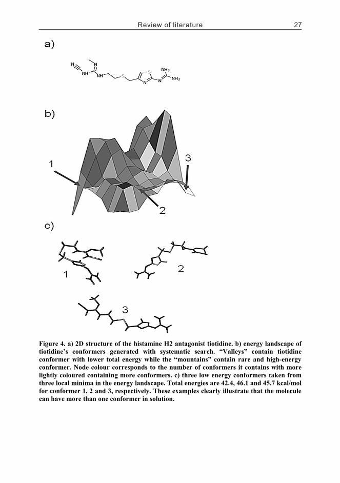
Review of literature 27
limited. A set of pharmacophoric features are identified that are thought to be important for binding. Distances between these features are used to restrict the conformational space that needs to be sampled for all the other molecules in the set. This has been shown to lead to similar results as with systematic search while being more than two orders of magnitude faster [39].
2.1.4 Force fields
Force fields are polynomial functions that are used for example in describing the conformational energy of the molecule or calculating the interaction energy between the molecule and a point in space near the molecule. The former type of a force field finds applications in optimization of the 3D geometry of the molecule. The latter type is useful in identifying the types of interactions the molecule can make with other molecules/chemical groups.
A typical force field for geometry optimization has the form of Equation 5 [52].
Equation 5
...+++++= elecvdwtorsbendstrtot EEEEEE
Here Etot is the total energy of the current conformer. Estr is the bond stretching term which compares the actual bond lengths of the conformer to the energetic optimum. Ebend in turn compares bond angles (bending) to their optimal values, Etors is the torsional term, Evdw controls that there are no major clashes of non-bonded atoms. Eelec is needed if charges are used to quantify electric attraction and repulsion.
Force fields need to be parameterized, i.e. proper values have to be assigned for constants in the equation. For this experimental data is needed. Different force fields (i.e. different sets of terms and parameters) have been developed for both small molecules and proteins. The distinction is not absolute with many of the force fields which can be used both for macromolecules and small molecules. For small molecules, noteworthy force fields include MM2/MM3 [53, 54], the Tripos force field [1] and the MMFF94s force field [55]. Among force fields used for modelling macromolecules, the most famous are the CHARMM [56], AMBER [57], OPLS [58] and GROMOS [59].
Figure 4. a) 2D structure of the histamine H2 antagonist tiotidine. b) energy landscape of
tiotidine’s conformers generated with systematic search. “Valleys” contain tiotidine
conformer with lower total energy while the “mountains” contain rare and high-energy
conformer. Node colour corresponds to the number of conformers it contains with more
lightly coloured containing more conformers. c) three low energy conformers taken from
three local minima in the energy landscape. Total energies are 42.4, 46.1 and 45.7 kcal/mol
for conformer 1, 2 and 3, respectively. These examples clearly illustrate that the molecule
can have more than one conformer in solution.

28 Review of literature
2.1.4.1 Molecule geometry optimization
Given a non-minimized 3D model of the molecule, the force field function is used in a step-by-step process to reach a minimum energy conformation. It should be noted that with a single starting conformer, it is not likely that the obtained minimum would correspond to the global energy minimum.
In the first phase when the conformer still has high energy, steepest descent approach is taken. Each atom is moved in one of the directions in space and the change in energy is recorded. Once all atoms have been iterated, the conformer is changed into the direction leading to the largest decrease in total energy (i.e. following the first derivate of the force field function). The process stops after a given number of steps or if the difference in energy is small enough.
Steepest descent is slow near the minimum state and fine-tuning of the conformation is done with an alternative method. One option for this is the conjugate gradient method where previous steps are recorded and they are used in deciding the next step [29]. This prevents the process from returning to an earlier state. Compared to steepest descent, conjugate gradients have the disadvantage of requiring more computational power and memory. However, this should not be a problem with modern computers. Like the steepest descent approach, conjugate gradient algorithm is terminated once a given number of steps have been taken or until the energy difference is small enough.
The two methods described above use only the first derivate of the force field to determine direction on the potential surface. Second derivate methods such as the Newton-Raphson method [29] use the derivative of the gradient (second derivative of the force field) to estimate where the minimum lies speeding up the minimization process. Storing the second derivate requires N2 of memory where N is the number of values of the gradient (first derivative) at a given point on the energy potential surface. Therefore the method should not be used for large systems such as proteins where the memory requirements would be too large.
2.1.4.2 Molecular interaction fields
Binding of a small molecule to a macromolecule usually occur with non-covalent interactions. The most important of these are the electrostatic, hydrogen bond, hydrophobic and van der Waals interactions. These can be modeled with the so called molecular interaction fields (MIF). MIF is a collection of evenly distributed grid nodes around the target molecule. Calculation of the MIF is started with a generation of a three dimensional grid around the molecule with equally spaced nodes. The interaction energy of the
target molecule and a chemical probe with specific interaction properties is measured at each node of the grid. A chemical probe represents common types of interactors such as hydrogen bond acceptors and donors found in small molecules.
MIFs for a given probe are visualized with 3D isoenergic contours (i.e. points in space with the same interaction potential). An example is given in Figure 5 for the topoisomerase 1 inhibitor irinotecan. Contours coloured in ivory represent space where a hydrogen bond acceptor makes favorable contacts with the molecule. Likewise the red contours show where a hydrogen bond donor could interact.
A number of programs have been developed to calculate MIFs such as HINT [60] and ISOSTAR/SUPERSTAR [61]. The most popular tool however must be GRID originally developed in the 1980s by Peter Goodford [62]. Here this software will be explained in more detail.
Figure 5. Regions surrounding irinotecan favourable for hydrogen-bond donors (red) and acceptors (ivory) as calculated with the GRID program.

Review of literature 29
2.1.4.1 Molecule geometry optimization
Given a non-minimized 3D model of the molecule, the force field function is used in a step-by-step process to reach a minimum energy conformation. It should be noted that with a single starting conformer, it is not likely that the obtained minimum would correspond to the global energy minimum.
In the first phase when the conformer still has high energy, steepest descent approach is taken. Each atom is moved in one of the directions in space and the change in energy is recorded. Once all atoms have been iterated, the conformer is changed into the direction leading to the largest decrease in total energy (i.e. following the first derivate of the force field function). The process stops after a given number of steps or if the difference in energy is small enough.
Steepest descent is slow near the minimum state and fine-tuning of the conformation is done with an alternative method. One option for this is the conjugate gradient method where previous steps are recorded and they are used in deciding the next step [29]. This prevents the process from returning to an earlier state. Compared to steepest descent, conjugate gradients have the disadvantage of requiring more computational power and memory. However, this should not be a problem with modern computers. Like the steepest descent approach, conjugate gradient algorithm is terminated once a given number of steps have been taken or until the energy difference is small enough.
The two methods described above use only the first derivate of the force field to determine direction on the potential surface. Second derivate methods such as the Newton-Raphson method [29] use the derivative of the gradient (second derivative of the force field) to estimate where the minimum lies speeding up the minimization process. Storing the second derivate requires N2 of memory where N is the number of values of the gradient (first derivative) at a given point on the energy potential surface. Therefore the method should not be used for large systems such as proteins where the memory requirements would be too large.
2.1.4.2 Molecular interaction fields
Binding of a small molecule to a macromolecule usually occur with non-covalent interactions. The most important of these are the electrostatic, hydrogen bond, hydrophobic and van der Waals interactions. These can be modeled with the so called molecular interaction fields (MIF). MIF is a collection of evenly distributed grid nodes around the target molecule. Calculation of the MIF is started with a generation of a three dimensional grid around the molecule with equally spaced nodes. The interaction energy of the
target molecule and a chemical probe with specific interaction properties is measured at each node of the grid. A chemical probe represents common types of interactors such as hydrogen bond acceptors and donors found in small molecules.
MIFs for a given probe are visualized with 3D isoenergic contours (i.e. points in space with the same interaction potential). An example is given in Figure 5 for the topoisomerase 1 inhibitor irinotecan. Contours coloured in ivory represent space where a hydrogen bond acceptor makes favorable contacts with the molecule. Likewise the red contours show where a hydrogen bond donor could interact.
A number of programs have been developed to calculate MIFs such as HINT [60] and ISOSTAR/SUPERSTAR [61]. The most popular tool however must be GRID originally developed in the 1980s by Peter Goodford [62]. Here this software will be explained in more detail.
Figure 5. Regions surrounding irinotecan favourable for hydrogen-bond donors (red) and acceptors (ivory) as calculated with the GRID program.

30 Review of literature
2.1.4.3 GRID
GRID is applicable for calculation of both small molecules and macromolecules. With the former, it is most useful when only active ligands but no structure of the target protein is known. MIFs for each of the small molecules are then calculated and common regions of interaction potential are identified. This gives indirect information of the properties of the macromolecular binding site. The results can then be applied for example in building a pharmacophore which, in turn, is used in virtual screening to find more potential binders.
For a protein active site, GRID can be used to determine favorable binding regions for a small molecule. These results can guide the design of ligands with complementary properties to the MIF. The information is also invaluable when optimizing existing ligands which might lack functional groups required for interaction with a specific region of the active site.
2.1.4.3.1 Calculating interaction fields with GRID
Like the typical force field for geometry optimization (Equation 5), the interaction energy of a probe with the molecule is calculated using a four term polynomial formula as shown in Equation 6.
Equation 6
SEEEE hbelvdwtot +++=
The first term Evdw represents the contribution of dispersion interaction. Even with non-polar atoms there is fluctuation of electron density around the nuclei. This results in induced small polarity when two atoms are in close contact with each other (i.e. the distance between the nuclei is the sum of the van der Waals radii of the two atoms). A contact closer than this leads to repulsion and a quick increase in interaction energy. GRID uses the Lennard-Jones function for calculating Evdw [Equation 7].
Equation 7
612 d
B
d
AEvdw −=
where d is the distance between the probe and the target atom. A and B are parameters based on van der Waals radii and polarizability of the probe and the atom.
The second term of the GRID force field represents electrostatic interaction. Treatment of the dielectric constant is more complicated than with most force fields and therefore this term [Equation 8] demands more discussion. The system is considered to consist of two homogenous phases with different dielectric coefficients: ζ = 4 for the target phase and ε = 80 for the solvent (water) phase.
Equation 8
+
+−+=qp
el
ssddK
pqE
4
)/()(12
εζεζζ
Terms p and q are the electrostatic charges of the probe and the atom of the target molecule. K is a constant and d is the distance between the probe and the target atom. Parameters sp and sq give the number of target atom nuclei (depth) within 4 Å of the probe and target atom, respectively. The closer the probe is to the target surface (inside a protein binding cavity for example), the larger the product 4spsq becomes effectively diminishing the latter term inside parentheses. This in turn means that the effective dielectric coefficient is very close to ζ. In contrast, the further the probe is from the target (meaning that sp
becomes zero), the greater the effective dielectric constant becomes modeling the dampening of electrostatic potential in water.
The third term quantifies hydrogen bonding. Here directionality of the interaction is important. GRID rotates the probe to optimize the interaction energy.
S is the entropy term introduced in GRID version 14 for the hydrophobic probe. Whenever order is introduced into the system (by constraining movement of atoms after ligand binding for example) entropy decreases. This has a negative impact on the binding event. This is at least partially compensated upon binding through release of highly structured water molecules into bulk water where their movement is less constrained which increases entropy. In GRID displacement of a water molecule from the binding site is assumed to be beneficial entropically. Each water molecule displaced gives an entropic contribution of -0.848 kcal/mol [63].
GRID also has a special probe type called DRY where the entropic component is used. DRY is used to identify hydrophobic regions on the target surface. Energy of the probe consists of three components [64]. The first one (WENT) is the constant -0.848 kcal/mol for displacing a structure water molecule from the target surface (see above). The second component (ELJ) quantifies induction

Review of literature 31
2.1.4.3 GRID
GRID is applicable for calculation of both small molecules and macromolecules. With the former, it is most useful when only active ligands but no structure of the target protein is known. MIFs for each of the small molecules are then calculated and common regions of interaction potential are identified. This gives indirect information of the properties of the macromolecular binding site. The results can then be applied for example in building a pharmacophore which, in turn, is used in virtual screening to find more potential binders.
For a protein active site, GRID can be used to determine favorable binding regions for a small molecule. These results can guide the design of ligands with complementary properties to the MIF. The information is also invaluable when optimizing existing ligands which might lack functional groups required for interaction with a specific region of the active site.
2.1.4.3.1 Calculating interaction fields with GRID
Like the typical force field for geometry optimization (Equation 5), the interaction energy of a probe with the molecule is calculated using a four term polynomial formula as shown in Equation 6.
Equation 6
SEEEE hbelvdwtot +++=
The first term Evdw represents the contribution of dispersion interaction. Even with non-polar atoms there is fluctuation of electron density around the nuclei. This results in induced small polarity when two atoms are in close contact with each other (i.e. the distance between the nuclei is the sum of the van der Waals radii of the two atoms). A contact closer than this leads to repulsion and a quick increase in interaction energy. GRID uses the Lennard-Jones function for calculating Evdw [Equation 7].
Equation 7
612 d
B
d
AEvdw −=
where d is the distance between the probe and the target atom. A and B are parameters based on van der Waals radii and polarizability of the probe and the atom.
The second term of the GRID force field represents electrostatic interaction. Treatment of the dielectric constant is more complicated than with most force fields and therefore this term [Equation 8] demands more discussion. The system is considered to consist of two homogenous phases with different dielectric coefficients: ζ = 4 for the target phase and ε = 80 for the solvent (water) phase.
Equation 8
+
+−+=qp
el
ssddK
pqE
4
)/()(12
εζεζζ
Terms p and q are the electrostatic charges of the probe and the atom of the target molecule. K is a constant and d is the distance between the probe and the target atom. Parameters sp and sq give the number of target atom nuclei (depth) within 4 Å of the probe and target atom, respectively. The closer the probe is to the target surface (inside a protein binding cavity for example), the larger the product 4spsq becomes effectively diminishing the latter term inside parentheses. This in turn means that the effective dielectric coefficient is very close to ζ. In contrast, the further the probe is from the target (meaning that sp
becomes zero), the greater the effective dielectric constant becomes modeling the dampening of electrostatic potential in water.
The third term quantifies hydrogen bonding. Here directionality of the interaction is important. GRID rotates the probe to optimize the interaction energy.
S is the entropy term introduced in GRID version 14 for the hydrophobic probe. Whenever order is introduced into the system (by constraining movement of atoms after ligand binding for example) entropy decreases. This has a negative impact on the binding event. This is at least partially compensated upon binding through release of highly structured water molecules into bulk water where their movement is less constrained which increases entropy. In GRID displacement of a water molecule from the binding site is assumed to be beneficial entropically. Each water molecule displaced gives an entropic contribution of -0.848 kcal/mol [63].
GRID also has a special probe type called DRY where the entropic component is used. DRY is used to identify hydrophobic regions on the target surface. Energy of the probe consists of three components [64]. The first one (WENT) is the constant -0.848 kcal/mol for displacing a structure water molecule from the target surface (see above). The second component (ELJ) quantifies induction

32 Review of literature
and dispersion interactions between the probe and the target. The value used here is the standard Lennard-Jones potential of a water molecule which the probe is simulated to replace. For the last component, the hydrogen bonding energy (EHB) is calculated that is lost when the water molecule is replaced with a hydrophobic component. For a non-polar surface this term is negligent but near a polar surface replacement of a water molecule with a hydrophobe carries a high enthalpic penalty. Final score for the DRY probe is WENT + ELJ – EHB where each component is a negative number. If the sum is negative the grid point is termed hydrophobic and hydrophilic otherwise.
2.1.4.3.2 GRID probes
The exact outcome of Equation 6 depends heavily on properties of the chemical probe being used. In addition to the special DRY probe discussed above, all the important functional group types are included and parameterized with experimental data. An extensive list of probes can be found in the GRID manual [65]. Some of the most commonly used probes are O1 which corresponds to an alkyl hydroxyl and is able to identify regions where a hydrogen bond donor can interact. N1 is the prototype probe for a hydrogen bond acceptor.
2.1.4.3.3 Applications of GRID
An early success story of using GRID came in 1993 when it was applied in rational design of zanamivir - an inhibitor of the influenza virus sialidase [66]. The molecule was later commercialized by Glaxo under the marketing name Relenza. The authors used GRID to probe the active site of sialidase and this led to critical changes in the structure of an earlier inhibitor.
More recently, a software called FLAP (Fingerprints for Ligands And Proteins) [67] has been developed for inspecting and comparing MIFs calculated with GRID. Each heavy atom is assigned into a general class depending on which GRID probe type it corresponds to. The atoms are used for generating 3- or 4-point 3D pharmacophores which are ultimately turned into a pharmacophore key that describes the combinations of atoms in the molecule and their mutual distances [Figure 6].
Figure 6. Three-point pharmacophores as generated with FLAP. Two triplets of functional groups in the molecules are identified. Mutual distances of these groups is recorded in a vector and used to represent the molecule. 4-point pharmacophores groups can be generated for three-dimensional structures to differentiate stereoisomers.
With protein active sites, the program first calculates a set of MIFs using probes mimicking the most important interaction types. The resulting interaction fields are analyzed and a set of site points with favorable interaction potential are identified. These points are combined – like with small molecules - into either 3- or 4-point 3D pharmacophores. Again, a pharmacophore key is generated describing all combinations of three or four site points of the active site.
The pharmacophore keys allow small molecules to be compared with active sites (docking), small molecules to be compared with other small molecules (ligand-based virtual screening) and protein relationships studies which are valuable in studying drug promiscuity.
2.2 Ligand-based virtual screening
A common assumption in drug design is that two compounds with similar chemical properties also exhibit similar biological effects [68]. This is the main principle and motivation of ligand-based virtual screening where a compound with interesting biological properties can be used as a query template in finding other compounds with the same properties. Since only one or more active small molecules are needed, ligand-based methods offer an alternative when no 3D target protein structure is available.
The definition of chemical similarity of two small molecules varies widely. In this chapter, three approaches for defining and quantifying chemical similarity are described: 2D fingerprints, 3D methods and pharmacophores.

Review of literature 33
and dispersion interactions between the probe and the target. The value used here is the standard Lennard-Jones potential of a water molecule which the probe is simulated to replace. For the last component, the hydrogen bonding energy (EHB) is calculated that is lost when the water molecule is replaced with a hydrophobic component. For a non-polar surface this term is negligent but near a polar surface replacement of a water molecule with a hydrophobe carries a high enthalpic penalty. Final score for the DRY probe is WENT + ELJ – EHB where each component is a negative number. If the sum is negative the grid point is termed hydrophobic and hydrophilic otherwise.
2.1.4.3.2 GRID probes
The exact outcome of Equation 6 depends heavily on properties of the chemical probe being used. In addition to the special DRY probe discussed above, all the important functional group types are included and parameterized with experimental data. An extensive list of probes can be found in the GRID manual [65]. Some of the most commonly used probes are O1 which corresponds to an alkyl hydroxyl and is able to identify regions where a hydrogen bond donor can interact. N1 is the prototype probe for a hydrogen bond acceptor.
2.1.4.3.3 Applications of GRID
An early success story of using GRID came in 1993 when it was applied in rational design of zanamivir - an inhibitor of the influenza virus sialidase [66]. The molecule was later commercialized by Glaxo under the marketing name Relenza. The authors used GRID to probe the active site of sialidase and this led to critical changes in the structure of an earlier inhibitor.
More recently, a software called FLAP (Fingerprints for Ligands And Proteins) [67] has been developed for inspecting and comparing MIFs calculated with GRID. Each heavy atom is assigned into a general class depending on which GRID probe type it corresponds to. The atoms are used for generating 3- or 4-point 3D pharmacophores which are ultimately turned into a pharmacophore key that describes the combinations of atoms in the molecule and their mutual distances [Figure 6].
Figure 6. Three-point pharmacophores as generated with FLAP. Two triplets of functional groups in the molecules are identified. Mutual distances of these groups is recorded in a vector and used to represent the molecule. 4-point pharmacophores groups can be generated for three-dimensional structures to differentiate stereoisomers.
With protein active sites, the program first calculates a set of MIFs using probes mimicking the most important interaction types. The resulting interaction fields are analyzed and a set of site points with favorable interaction potential are identified. These points are combined – like with small molecules - into either 3- or 4-point 3D pharmacophores. Again, a pharmacophore key is generated describing all combinations of three or four site points of the active site.
The pharmacophore keys allow small molecules to be compared with active sites (docking), small molecules to be compared with other small molecules (ligand-based virtual screening) and protein relationships studies which are valuable in studying drug promiscuity.
2.2 Ligand-based virtual screening
A common assumption in drug design is that two compounds with similar chemical properties also exhibit similar biological effects [68]. This is the main principle and motivation of ligand-based virtual screening where a compound with interesting biological properties can be used as a query template in finding other compounds with the same properties. Since only one or more active small molecules are needed, ligand-based methods offer an alternative when no 3D target protein structure is available.
The definition of chemical similarity of two small molecules varies widely. In this chapter, three approaches for defining and quantifying chemical similarity are described: 2D fingerprints, 3D methods and pharmacophores.

34 Review of literature
2.2.1 2D similarity search
2.2.1.1 Substructure searching
The most widely used approach for measuring the chemical similarity of two small molecules is to compare their 2D topology. The oldest approach is sub-structure search where the presence of a certain substructure (e.g. steroid ring system) is queried across a database of molecules. However, substructure searching is an NP-complete problem meaning that the time required for the search grows very fast as the size of the molecules grows.
Due to the poor time performance of substructure searching, faster methods are required. A commonly used solution is to employ so called structure keys. These are fixed-length sets where each component of the key set corresponds to a pre-defined substructure. If the sub-structure is found in the molecule, the set component corresponding to it is set to 1 and 0 if the substructure is not found.
For a large database, structure keys can be generated “up-front” without the need to repeat the process every time the database is queried. All that remains to be done later is to compare the strings of zeros and ones between the query and the database keysets which is easy computationally. In addition to substructuresearching, structure keys can be used for similarity searching as exemplified in the paper introducing the new version of the widely used MDL keys [69].
2.2.1.2 Path Fingerprints
The main problem with structure keys is their context-dependency. A given set of pre-determined structure keys can work fine for one application and be nearly useless for another. This has been solved with the use of molecular fingerprints which today is the most used method for comparing small molecules. Fingerprints are applicable to a much wider set of structures as they do not encode the existence of pre-determined substructures. Only the atom-atom connectivity of the input molecule is needed for generating the fingerprint.
Path Fingerprints are generated by the systematic path analysis of bonds connecting the atoms of the molecule. All paths between two atoms in the molecule are iterated up to a given maximum length. The process is exhaustive meaning that every possible feature (i.e. path) in the molecule is generated. An example of the process is given in Figure 7. Each path generated is a fragment identified with an integer. To make comparison of features efficient, a constant length binary fingerprint is derived for each molecule (e.g. 1024 bits). A computational technique called hashing is used to map each path identifier into
certain sets of bits in the fingerprint. Since each path corresponds to a large integer, this can be used as a seed in a pseudo-random number generator. Output tells which fingerprint bits are to be set to 1’s. Usually each feature corresponds to only a few bits. An individual bit can be set to on by a number of different features but no two features correspond to exactly the same set of bits [70].
Unlike with structure keys, a given hashed fingerprint bit does not have a direct correspondence with a certain substructure or path in the molecule. Instead, molecular fingerprints should be understood as their biological counterparts: all people have unique fingerprints but they cannot be used to make any conclusions of the properties of the individual such as height or eye color.
Figure 7. Illustration of hashed path fingerprints. Atom-atom paths are first identified from the molecule taking only heavy (non-hydrogen) atoms in account. Each path fragment corresponds to an integer value which given as input for a hash function that turns one or more bits on in a fixed length binary fingerprint (10 bits in this example).

Review of literature 35
2.2.1 2D similarity search
2.2.1.1 Substructure searching
The most widely used approach for measuring the chemical similarity of two small molecules is to compare their 2D topology. The oldest approach is sub-structure search where the presence of a certain substructure (e.g. steroid ring system) is queried across a database of molecules. However, substructure searching is an NP-complete problem meaning that the time required for the search grows very fast as the size of the molecules grows.
Due to the poor time performance of substructure searching, faster methods are required. A commonly used solution is to employ so called structure keys. These are fixed-length sets where each component of the key set corresponds to a pre-defined substructure. If the sub-structure is found in the molecule, the set component corresponding to it is set to 1 and 0 if the substructure is not found.
For a large database, structure keys can be generated “up-front” without the need to repeat the process every time the database is queried. All that remains to be done later is to compare the strings of zeros and ones between the query and the database keysets which is easy computationally. In addition to substructuresearching, structure keys can be used for similarity searching as exemplified in the paper introducing the new version of the widely used MDL keys [69].
2.2.1.2 Path Fingerprints
The main problem with structure keys is their context-dependency. A given set of pre-determined structure keys can work fine for one application and be nearly useless for another. This has been solved with the use of molecular fingerprints which today is the most used method for comparing small molecules. Fingerprints are applicable to a much wider set of structures as they do not encode the existence of pre-determined substructures. Only the atom-atom connectivity of the input molecule is needed for generating the fingerprint.
Path Fingerprints are generated by the systematic path analysis of bonds connecting the atoms of the molecule. All paths between two atoms in the molecule are iterated up to a given maximum length. The process is exhaustive meaning that every possible feature (i.e. path) in the molecule is generated. An example of the process is given in Figure 7. Each path generated is a fragment identified with an integer. To make comparison of features efficient, a constant length binary fingerprint is derived for each molecule (e.g. 1024 bits). A computational technique called hashing is used to map each path identifier into
certain sets of bits in the fingerprint. Since each path corresponds to a large integer, this can be used as a seed in a pseudo-random number generator. Output tells which fingerprint bits are to be set to 1’s. Usually each feature corresponds to only a few bits. An individual bit can be set to on by a number of different features but no two features correspond to exactly the same set of bits [70].
Unlike with structure keys, a given hashed fingerprint bit does not have a direct correspondence with a certain substructure or path in the molecule. Instead, molecular fingerprints should be understood as their biological counterparts: all people have unique fingerprints but they cannot be used to make any conclusions of the properties of the individual such as height or eye color.
Figure 7. Illustration of hashed path fingerprints. Atom-atom paths are first identified from the molecule taking only heavy (non-hydrogen) atoms in account. Each path fragment corresponds to an integer value which given as input for a hash function that turns one or more bits on in a fixed length binary fingerprint (10 bits in this example).

36 Review of literature
2.2.1.3 Extended Connectivity Fingerprints
Another breed of fingerprints are the so called extended connectivity fingerprints (ECFP) [71] implemented in the Pipeline Pilot software [72]. Sharing some resemblance to the path fingerprints described above, ECFPs are generated by iteratively taking each atom as a starting point for feature generation.
Whereas path fingerprints generate the features as a function of a path between two atoms in the molecule, ECFPs use the complete neighborhood around each atom. An atom neighborhood includes all the atoms within a given distance threshold from the central atom plus all the bonds connecting them. Atom and bond types within the neighborhood are written in an array of number pairs. In each number pair the first number describes the bond type and the second number gives the atom type the bond leads to. This array is transformed into an
integer value specific for the fragment. Finally the integer is given as input for a hashing function which turns certain set of bits on in a fixed-length binary fingerprint.
2.2.1.4 Similarity metrics
Once fingerprints have been calculated for the database, their similarity needs to be calculated. Several similarity metrics have been proposed and used over the years and Table 1 gives an overview of the most common ones.
The most commonly used similarity metric for calculating fingerprint similarity is the Tanimoto similarity (first row in Table 1) which is defined as the ratio of bits set on in both fingerprints divided by the number of distinct bits set on in either fingerprint. An important point to notice here is that bits set to zero in both fingerprints are ignored. This is because most of the bits are usually zeros in a given fingerprint. Including them in the equation would undermine the ability of the metric to differentiate similar compounds from dissimilar ones.
One problem often associated with metrics such as those listed in Table 1 is size-bias, i.e. tendency to systematically favor small/large compounds [73]. This effect was studied by Holliday et al [74]. They found that most of the metrics studied exhibited bias to either small or large compounds. As an exception, the Modified Tanimoto metric [75] was found to be largely unaffected by compound size.
Table 1. Common similarity metrics for binary fingerprints. Number of fingerprints turned on in the fingerprint for the first and the second molecule are given as a and b, respectively and c is the number of bits turned on in the both fingerprints. Total number of bits contained in a fingerprint is m.
Metric Expression Metric Expression
Tanimoto
cba
c
−+Russell-Rao m
c
Cosine
ab
c Forbes
ab
cm
Hamming cba 2−+
2.2.2 3D methods
The 2D methods described above are popular largely due to their speed and simplicity. A major disadvantage in their use is the type of results they produce in a virtual screening campaign. The high scoring hits tend to have the same structural features and scaffold as the query molecule. This is fine as long as structural analogs are sought. Such a situation could arise when an interesting hit molecule has been found in a high throughput screen. Then one wants to query a database for more compounds that share the same scaffold as the original hit.
However, often the motivation for a virtual screening campaign is to find compounds that share the biological activity of the query molecule but do not have the same scaffold (“scaffold hopping”) [76]. One reason for this can be that the original molecule and its analogs are protected by patents. Alternatively there can be toxicity problems with the original compound. Finding a novel lead structure with scaffold hopping can potentially alleviate both of these problems.
An example of such a case is given in Figure 8 which has 2D structures of three phosphodiesterase 5 (PDE5) inhibitors all used in the treatment for erectile dysfunction. Two of the molecules (Sildenafil and Vardenafil) differ by only two small changes in their structures. In contrast, Tadalafil exhibit a case of scaffold hopping having a completely different 2D structure but still sharing the biological activity of the other two (PDE5 inhibition). The pharmacokinetic properties of Tadalafil are superior to the other two compounds (improved half-life [77] and absorption not influenced by food intake [78]) making it a competitive alternative to Sildenafil and Vardenafil.

Review of literature 37
2.2.1.3 Extended Connectivity Fingerprints
Another breed of fingerprints are the so called extended connectivity fingerprints (ECFP) [71] implemented in the Pipeline Pilot software [72]. Sharing some resemblance to the path fingerprints described above, ECFPs are generated by iteratively taking each atom as a starting point for feature generation.
Whereas path fingerprints generate the features as a function of a path between two atoms in the molecule, ECFPs use the complete neighborhood around each atom. An atom neighborhood includes all the atoms within a given distance threshold from the central atom plus all the bonds connecting them. Atom and bond types within the neighborhood are written in an array of number pairs. In each number pair the first number describes the bond type and the second number gives the atom type the bond leads to. This array is transformed into an
integer value specific for the fragment. Finally the integer is given as input for a hashing function which turns certain set of bits on in a fixed-length binary fingerprint.
2.2.1.4 Similarity metrics
Once fingerprints have been calculated for the database, their similarity needs to be calculated. Several similarity metrics have been proposed and used over the years and Table 1 gives an overview of the most common ones.
The most commonly used similarity metric for calculating fingerprint similarity is the Tanimoto similarity (first row in Table 1) which is defined as the ratio of bits set on in both fingerprints divided by the number of distinct bits set on in either fingerprint. An important point to notice here is that bits set to zero in both fingerprints are ignored. This is because most of the bits are usually zeros in a given fingerprint. Including them in the equation would undermine the ability of the metric to differentiate similar compounds from dissimilar ones.
One problem often associated with metrics such as those listed in Table 1 is size-bias, i.e. tendency to systematically favor small/large compounds [73]. This effect was studied by Holliday et al [74]. They found that most of the metrics studied exhibited bias to either small or large compounds. As an exception, the Modified Tanimoto metric [75] was found to be largely unaffected by compound size.
Table 1. Common similarity metrics for binary fingerprints. Number of fingerprints turned on in the fingerprint for the first and the second molecule are given as a and b, respectively and c is the number of bits turned on in the both fingerprints. Total number of bits contained in a fingerprint is m.
Metric Expression Metric Expression
Tanimoto
cba
c
−+Russell-Rao m
c
Cosine
ab
c Forbes
ab
cm
Hamming cba 2−+
2.2.2 3D methods
The 2D methods described above are popular largely due to their speed and simplicity. A major disadvantage in their use is the type of results they produce in a virtual screening campaign. The high scoring hits tend to have the same structural features and scaffold as the query molecule. This is fine as long as structural analogs are sought. Such a situation could arise when an interesting hit molecule has been found in a high throughput screen. Then one wants to query a database for more compounds that share the same scaffold as the original hit.
However, often the motivation for a virtual screening campaign is to find compounds that share the biological activity of the query molecule but do not have the same scaffold (“scaffold hopping”) [76]. One reason for this can be that the original molecule and its analogs are protected by patents. Alternatively there can be toxicity problems with the original compound. Finding a novel lead structure with scaffold hopping can potentially alleviate both of these problems.
An example of such a case is given in Figure 8 which has 2D structures of three phosphodiesterase 5 (PDE5) inhibitors all used in the treatment for erectile dysfunction. Two of the molecules (Sildenafil and Vardenafil) differ by only two small changes in their structures. In contrast, Tadalafil exhibit a case of scaffold hopping having a completely different 2D structure but still sharing the biological activity of the other two (PDE5 inhibition). The pharmacokinetic properties of Tadalafil are superior to the other two compounds (improved half-life [77] and absorption not influenced by food intake [78]) making it a competitive alternative to Sildenafil and Vardenafil.

38 Review of literature
The current and the two following chapters (pharmacophores and docking) introduce virtual screening methods that all can be used to perform scaffold hopping. Common feature for them all is that the 2D structures of the compounds are not taken into account explicitly. Rather, compounds are compared by quantifying their shape overlap and interaction field similarity. In order to bind the target strongly, shape and charge distribution of the small molecule must complement those of the binding site in the macromolecule. From the point of view of the macromolecule, the explicit 2D structure of the small molecule is irrelevant.
2.2.2.1 General idea of 3D overlay tools
All the 3D overlay tools described in this chapter follow the same basic principle: one or more molecules are used as template molecules (sometimes also called query or target molecules) on which database compounds are overlaid and scored. The template molecule should be in an energy minimized conformation. Alternatively, the bioactive conformation from a protein co-crystal structure can be used when available [79, 80].
Conformers for the database molecules must be pre-calculated for most programs. Generation of conformers is described above and is not discussed here. In addition, some programs require appropriate point charges to be pre-calculated for both the template and the database molecules if electrostatic field similarity is quantified.
Figure 8. 2D structures of three drug molecules all binding to phosphodiesterase 5. Vardenafil and Sildenafil are very similar structurally and also share the same pharmacokinetic properties. Tadalafil in contrast has a very different structure and also pharmacokinetic properties superior to the former two.
2.2.2.2 Types of 3D overlay tools
Methods based on interaction grids are one of the main types of 3D overlay methods. They build a constant-spaced grid around the 3D model of the molecule. The interaction energy between the molecule and each grid node is calculated using a force field of choice. It is important to note that this is an approximation of the force fields which are continuous functions. Therefore the grid spacing has to be sufficiently dense so that no important features of the force field are missed. A plethora of probes (interaction types) have been developed over the years.
A method used in all the publications of this thesis, BRUTUS, belongs to the family of grid-based tools [81-83]. Field types implemented in BRUTUS are van der Waals and electrostatic fields which are combined in one combo-field type to speed-up overlaying. The fields are combined by assigning points inside the van der Waals radii as a constant value and using calculated values outside the radii. The program quantifies chemical similarity of two overlaid compounds as function of complementary of their grid nodes. Figure 9 gives a simplified schematic illustration of how BRUTUS superposes two molecules.
Grids are not the only possibility to compare molecules based on their interaction fields. Another option is to calculate the interaction potentials in selected points in space close to the compound surface. Based on these calculations, local interaction energy minima are then chosen to represent the complete interaction field. Overlay of two molecules is achieved by optimizing the overlap of these minima. This is the approach taken in FieldCompare [84, 85] and ShaEP [86].
As noted above, grid-based methods suffer from approximating the force field(s). An alternative tool to compare interaction potentials is by Gaussian functions. Each atom of the molecule has a set of Gaussian functions associated with it. The interaction potential of a point in space around the molecule can be calculated as a sum of functions of all atoms. Comparison of two molecules can be quantified by a simple integration of their respective Gaussians.
A popular tool employing Gaussians is ROCS by OpenEye Software [87]. Gaussians are especially adept in representing the volume (shape) of the molecule. Therefore one important component of ROCS similarity is shape overlap. A second component employed in ROCS scoring is the Colorscore which quantifies the relative overlap of functional groups.

Review of literature 39
The current and the two following chapters (pharmacophores and docking) introduce virtual screening methods that all can be used to perform scaffold hopping. Common feature for them all is that the 2D structures of the compounds are not taken into account explicitly. Rather, compounds are compared by quantifying their shape overlap and interaction field similarity. In order to bind the target strongly, shape and charge distribution of the small molecule must complement those of the binding site in the macromolecule. From the point of view of the macromolecule, the explicit 2D structure of the small molecule is irrelevant.
2.2.2.1 General idea of 3D overlay tools
All the 3D overlay tools described in this chapter follow the same basic principle: one or more molecules are used as template molecules (sometimes also called query or target molecules) on which database compounds are overlaid and scored. The template molecule should be in an energy minimized conformation. Alternatively, the bioactive conformation from a protein co-crystal structure can be used when available [79, 80].
Conformers for the database molecules must be pre-calculated for most programs. Generation of conformers is described above and is not discussed here. In addition, some programs require appropriate point charges to be pre-calculated for both the template and the database molecules if electrostatic field similarity is quantified.
Figure 8. 2D structures of three drug molecules all binding to phosphodiesterase 5. Vardenafil and Sildenafil are very similar structurally and also share the same pharmacokinetic properties. Tadalafil in contrast has a very different structure and also pharmacokinetic properties superior to the former two.
2.2.2.2 Types of 3D overlay tools
Methods based on interaction grids are one of the main types of 3D overlay methods. They build a constant-spaced grid around the 3D model of the molecule. The interaction energy between the molecule and each grid node is calculated using a force field of choice. It is important to note that this is an approximation of the force fields which are continuous functions. Therefore the grid spacing has to be sufficiently dense so that no important features of the force field are missed. A plethora of probes (interaction types) have been developed over the years.
A method used in all the publications of this thesis, BRUTUS, belongs to the family of grid-based tools [81-83]. Field types implemented in BRUTUS are van der Waals and electrostatic fields which are combined in one combo-field type to speed-up overlaying. The fields are combined by assigning points inside the van der Waals radii as a constant value and using calculated values outside the radii. The program quantifies chemical similarity of two overlaid compounds as function of complementary of their grid nodes. Figure 9 gives a simplified schematic illustration of how BRUTUS superposes two molecules.
Grids are not the only possibility to compare molecules based on their interaction fields. Another option is to calculate the interaction potentials in selected points in space close to the compound surface. Based on these calculations, local interaction energy minima are then chosen to represent the complete interaction field. Overlay of two molecules is achieved by optimizing the overlap of these minima. This is the approach taken in FieldCompare [84, 85] and ShaEP [86].
As noted above, grid-based methods suffer from approximating the force field(s). An alternative tool to compare interaction potentials is by Gaussian functions. Each atom of the molecule has a set of Gaussian functions associated with it. The interaction potential of a point in space around the molecule can be calculated as a sum of functions of all atoms. Comparison of two molecules can be quantified by a simple integration of their respective Gaussians.
A popular tool employing Gaussians is ROCS by OpenEye Software [87]. Gaussians are especially adept in representing the volume (shape) of the molecule. Therefore one important component of ROCS similarity is shape overlap. A second component employed in ROCS scoring is the Colorscore which quantifies the relative overlap of functional groups.

40 Review of literature
2.2.2.3 Overlay optimization
All overlay tools need a set of initial overlays as starting points to begin with. The database molecule is then rotated and translated along the gradient until a local minimum is reached. An ensemble of different initial overlays is needed to make sure one of these local minima is also the global minimum with a reasonable probability. Having a large number of starting overlays improves this probability but requires more computational time.
Different programs solve the problem of initial overlays in different ways. ROCS uses only a few initial starting points where the molecules have been aligned along their inertial axes [88]. This has been shown to be enough to find the global optimal overlay in most cases [89]. Software utilizing graphs such as ShaEP [86] and FieldScreen [84, 85] derive a set of initial overlays based on maximal subgraphs of full graphs of the molecules where nodes represent interaction potential minima.
BRUTUS employs a very large set of initial overlays which are then pruned for final optimization. First the grid of a database molecule is translated using step size of 1 Å within the grid of the template molecule. Starting from these positions, the grid of the database molecule is rotated with step size of 30 degrees each of which leads to an initial alignment.
After the set of initial alignments have been derived, all that remains is to optimize the overlay towards the local minimum. Once this has been done for each initial alignment the software reports one or more of the top solutions for further analysis [81-83].
Figure 9. Schematic illustration of BRUTUS overlay algorithm. a) first a grid is built around the molecule and electrostatic potential between a grid node (intersection of lines in this illustration) and all heavy atoms of the molecule is calculated. Grid points falling inside the van der Waals radius of the molecule (illustrated with oval shapes) are assigned a constant value. b) the two grids are overlaid by keeping the template grid static while rotating and translating the grid of the database molecule. The aim is to maximize similarity of node pairs from the two grids located closely in space.

Review of literature 41
2.2.2.3 Overlay optimization
All overlay tools need a set of initial overlays as starting points to begin with. The database molecule is then rotated and translated along the gradient until a local minimum is reached. An ensemble of different initial overlays is needed to make sure one of these local minima is also the global minimum with a reasonable probability. Having a large number of starting overlays improves this probability but requires more computational time.
Different programs solve the problem of initial overlays in different ways. ROCS uses only a few initial starting points where the molecules have been aligned along their inertial axes [88]. This has been shown to be enough to find the global optimal overlay in most cases [89]. Software utilizing graphs such as ShaEP [86] and FieldScreen [84, 85] derive a set of initial overlays based on maximal subgraphs of full graphs of the molecules where nodes represent interaction potential minima.
BRUTUS employs a very large set of initial overlays which are then pruned for final optimization. First the grid of a database molecule is translated using step size of 1 Å within the grid of the template molecule. Starting from these positions, the grid of the database molecule is rotated with step size of 30 degrees each of which leads to an initial alignment.
After the set of initial alignments have been derived, all that remains is to optimize the overlay towards the local minimum. Once this has been done for each initial alignment the software reports one or more of the top solutions for further analysis [81-83].
Figure 9. Schematic illustration of BRUTUS overlay algorithm. a) first a grid is built around the molecule and electrostatic potential between a grid node (intersection of lines in this illustration) and all heavy atoms of the molecule is calculated. Grid points falling inside the van der Waals radius of the molecule (illustrated with oval shapes) are assigned a constant value. b) the two grids are overlaid by keeping the template grid static while rotating and translating the grid of the database molecule. The aim is to maximize similarity of node pairs from the two grids located closely in space.

42 Review of literature
2.3 Pharmacophore modeling
2.3.1 Definition
The official IUPAC (International Union of Pure and Applied Chemistry) definition from 1998 for pharmacophores is as follows [90] :
A pharmacophore is the ensemble of steric and electronic features that is
necessary to ensure the optimal supramolecular interactions with a specific
biological target structure to trigger (or to block) its biological response.
The pharmacophore is an abstract concept [91] describing a set of interactions required to bind a given cavity. A common way to visualize a pharmacophore is as a set of spatially arranged spheres with certain type and diameter. The spheres are commonly called (pharmacophore) features.
Common feature types are hydrophobic, hydrogen bond acceptor, hydrogen bond donor, positively ionizable and negatively ionizable groups. Each feature therefore describes the target binding site, e.g. a hydrophobic feature corresponds to a hydrophobic protein side chain(s) in the cavity, a hydrogen bond acceptor feature has hydrogen bond donating counterpart in the protein. Hydrogen bond acceptor and donor features usually have direction as a parameter.
The starting point for a pharmacophore model can be a set of active molecules known to bind the same cavity or a co-crystal structure of an active ligand bound to the target [92].
2.3.2 Ligand-based pharmacophore modeling
Probably the most common used approach for pharmacophore model generation is to start from a set of active small molecules. Some pharmacophore modeling tools require pre-calculated 3D molecule conformers [93] whereas some tools are able to generate them on-the-fly [94].
Tools such as GASP [94] require a template molecule on which the rest of the compounds are overlaid based on pharmacophore features the compounds have in common. Usually the most rigid compound is used as a template. CATALYST [47] requires the user to choose one reference molecule but the actual conformer of the reference used in the final model depends how well the other molecules can be overlaid on it. On the other hand, GALAHAD [93] does not require a template to be specified.
Tools such as CATALYST allow the user to reduce the mapping constraints, e.g. all molecules in the training set are not required to map to each and every feature of the model. Additionally some molecules in the set can be completely excluded from the model. This is practical if there are molecules that exert their activity through a different binding mode.
Excluded volumes can also be included in the pharmacophore models. They correspond to regions in space occupied by protein heavy atoms and can be used to avoid steric clashes. Inactive molecules that might otherwise fulfill the pharmacophore features can be excluded if they contain atoms in these regions. Toba et al. [95] described an extension to CATALYST where the information from inactive molecules is used to generate excluded volumes and no information of 3D structure of the target protein is needed.
2.3.3 Protein-based pharmacophore modeling
Another strategy for pharmacophore generation is to use a protein structure co-crystallized with a ligand [91, 92]. The largest public repository for protein structures is the Protein Data Bank (PDB) [96]. By analyzing the interactions the co-crystallized ligand makes with its target, it is possible to derive a pharmacophore. One automated tool for the job is LigandScout [92]. The software reads in the co-crystal structure and fixes errors that are common in PDB files. The derived model can also be edited manually and finally exported for virtual screening with CATALYST for instance. Since the coordinates of the proteins heavy atoms are explicitly known, exclusion spheres can be included to avoid ligand-protein steric clashes.
If only an apo structure of the target exists, hot spot analysis can be employed to identify regions of the cavity where the functional group of a given ligand could form a strong interaction [91]. The cavity is first embedded in a grid and the interaction energy of each grid node and the protein is measured with a set of probes each representing a certain type of interaction type. The energy minima found in this way can be converted into pharmacophore features. One option for calculating the energies is GRID [62]. Another tool with the same principle is SuperStar [61].
Once the pharmacophore model has been constructed it can be used for virtual screening of small molecules. Many tools such as CATALYST and Phase [97] are able to do this without the need for additional software. Before applying the models for virtual screening of large databases they still need validation with known actives not used in building the models and appropriate decoy (inactive) molecules. The validation issues are discussed later in the thesis.
Review of literature 43
2.3 Pharmacophore modeling
2.3.1 Definition
The official IUPAC (International Union of Pure and Applied Chemistry) definition from 1998 for pharmacophores is as follows [90] :
A pharmacophore is the ensemble of steric and electronic features that is
necessary to ensure the optimal supramolecular interactions with a specific
biological target structure to trigger (or to block) its biological response.
The pharmacophore is an abstract concept [91] describing a set of interactions required to bind a given cavity. A common way to visualize a pharmacophore is as a set of spatially arranged spheres with certain type and diameter. The spheres are commonly called (pharmacophore) features.
Common feature types are hydrophobic, hydrogen bond acceptor, hydrogen bond donor, positively ionizable and negatively ionizable groups. Each feature therefore describes the target binding site, e.g. a hydrophobic feature corresponds to a hydrophobic protein side chain(s) in the cavity, a hydrogen bond acceptor feature has hydrogen bond donating counterpart in the protein. Hydrogen bond acceptor and donor features usually have direction as a parameter.
The starting point for a pharmacophore model can be a set of active molecules known to bind the same cavity or a co-crystal structure of an active ligand bound to the target [92].
2.3.2 Ligand-based pharmacophore modeling
Probably the most common used approach for pharmacophore model generation is to start from a set of active small molecules. Some pharmacophore modeling tools require pre-calculated 3D molecule conformers [93] whereas some tools are able to generate them on-the-fly [94].
Tools such as GASP [94] require a template molecule on which the rest of the compounds are overlaid based on pharmacophore features the compounds have in common. Usually the most rigid compound is used as a template. CATALYST [47] requires the user to choose one reference molecule but the actual conformer of the reference used in the final model depends how well the other molecules can be overlaid on it. On the other hand, GALAHAD [93] does not require a template to be specified.
Tools such as CATALYST allow the user to reduce the mapping constraints, e.g. all molecules in the training set are not required to map to each and every feature of the model. Additionally some molecules in the set can be completely excluded from the model. This is practical if there are molecules that exert their activity through a different binding mode.
Excluded volumes can also be included in the pharmacophore models. They correspond to regions in space occupied by protein heavy atoms and can be used to avoid steric clashes. Inactive molecules that might otherwise fulfill the pharmacophore features can be excluded if they contain atoms in these regions. Toba et al. [95] described an extension to CATALYST where the information from inactive molecules is used to generate excluded volumes and no information of 3D structure of the target protein is needed.
2.3.3 Protein-based pharmacophore modeling
Another strategy for pharmacophore generation is to use a protein structure co-crystallized with a ligand [91, 92]. The largest public repository for protein structures is the Protein Data Bank (PDB) [96]. By analyzing the interactions the co-crystallized ligand makes with its target, it is possible to derive a pharmacophore. One automated tool for the job is LigandScout [92]. The software reads in the co-crystal structure and fixes errors that are common in PDB files. The derived model can also be edited manually and finally exported for virtual screening with CATALYST for instance. Since the coordinates of the proteins heavy atoms are explicitly known, exclusion spheres can be included to avoid ligand-protein steric clashes.
If only an apo structure of the target exists, hot spot analysis can be employed to identify regions of the cavity where the functional group of a given ligand could form a strong interaction [91]. The cavity is first embedded in a grid and the interaction energy of each grid node and the protein is measured with a set of probes each representing a certain type of interaction type. The energy minima found in this way can be converted into pharmacophore features. One option for calculating the energies is GRID [62]. Another tool with the same principle is SuperStar [61].
Once the pharmacophore model has been constructed it can be used for virtual screening of small molecules. Many tools such as CATALYST and Phase [97] are able to do this without the need for additional software. Before applying the models for virtual screening of large databases they still need validation with known actives not used in building the models and appropriate decoy (inactive) molecules. The validation issues are discussed later in the thesis.
44 Review of literature
The output from mapping a small molecule on the pharmacophore can be either qualitative (binds/does not bind) or quantitative. In the latter case compounds passing the pharmacophore filter can be ranked for further filtering.
2.4 Docking
Placing a small molecule in a three dimensional model of the protein binding site (docking) is one of the most widely used virtual screening techniques. Docking can be applied to screen a database for novel binders (virtual screening). Another potential application is the identification of a putative binding mode for a known active molecule. This is valuable when deciding which analogs to synthesize and test next (lead development). The two major components of any docking tool are the docking algorithm and the scoring function which are introduced in the following chapters.
2.4.1 Docking algorithms
How the pose prediction step (i.e. predicting which interactions the ligand makes with the protein) is performed depends on the docking software used. The most popular options include genetic algorithms and the incremental construction of the bound pose.
Genetic algorithm is implemented in the widely used GOLD docking tool [98]. Each binding pose of a ligand including its conformations is expressed as a string of values (termed chromosome). Initially, a set of chromosome populations (“islands”) is randomly generated. Each chromosome is given a fitness value with a scoring function that describes how well the ligand fits into the binding cavity. Once the whole population on an island has been scored, three evolutionary operators can be applied to generate the next generation of chromosomes. With cross-over two parent chromosomes within an island swap parts of their chromosomes to generate two child chromosomes. With mutation some properties of a single parent chromosome are altered to generate a new child chromosome. With migration a chromosome is copied to another population island. For cross-over and mutation the parent(s) are chosen randomly with a bias towards chromosomes with high fit values. The resulting children replace the least fit members of the population. Relative probability of each operator varies with migration being rare (5 % by default) and cross-over and mutation more equally probable. This loop is repeated for a number of user-defined generations. In the end only solutions with high fit value should remain in each island leading to identification of the correct binding mode.
In the other popular docking algorithm – incremental construction – the ligand is split in rigid fragments by cutting its rotatable bonds. One of these fragments,
termed base fragment, is first placed into the binding cavity. The way the base fragment is placed depends on the software implementing the algorithm. Dock [99] analyzes the binding site before any docking is done to identify a set of non-overlapping spheres each corresponding to a ligand heavy atom. The base fragment is placed in a way to match these spheres. FlexX [100] is another docking program using incremental construction. Here the base fragment is placed in a way to have the ligand make at least three interactions with the protein. With both programs the remaining fragments are attached one by one once the base fragment has been placed. It is usually possible to place the base fragment in more than one way. Accordingly this leads to more than one possible binding pose. The solutions are scored to identify the top binding poses for further analysis.
The algorithms introduced above require only one conformer of the molecule as its conformational space is explored automatically during docking. With other programs the user has to generate the ensemble of conformers before running the docking algorithm. For example, FRED [101] treats the ligand rigid meaning that given a single input conformer it is unlikely to find the correct binding mode. FRED performs exhaustive docking with each input conformer by rotating and translating the molecule in the binding site. This leads to a large set of putative binding modes. These are initially filtered by excluding every solution not residing inside a pre-defined volume defining the binding site. Additionally at least one heavy atom is required to be within a smaller core volume. The remaining poses are scored with one of the scoring functions implemented in the program. A number of top scoring (by default 100) poses are retained which are used for further analysis such as the consensus scoring with additional scoring functions.
The top scoring binding pose given by any of the tools can still be non-optimal. Therefore it is recommended to optimize the ligand-protein geometry with a force field. For example, FRED uses the MMFF force field [55] to do this but due to the computational expense of minimization it is not run by default.
2.4.2 Scoring functions
The other critical component of any docking software is the scoring function. The objective of any scoring function is to estimate the free energy of binding for a ligand in a given binding pose. This can be expressed mathematically by the fundamental thermodynamic Equation 9:
Equation 9
STHG ∆−∆=∆

Review of literature 45
The output from mapping a small molecule on the pharmacophore can be either qualitative (binds/does not bind) or quantitative. In the latter case compounds passing the pharmacophore filter can be ranked for further filtering.
2.4 Docking
Placing a small molecule in a three dimensional model of the protein binding site (docking) is one of the most widely used virtual screening techniques. Docking can be applied to screen a database for novel binders (virtual screening). Another potential application is the identification of a putative binding mode for a known active molecule. This is valuable when deciding which analogs to synthesize and test next (lead development). The two major components of any docking tool are the docking algorithm and the scoring function which are introduced in the following chapters.
2.4.1 Docking algorithms
How the pose prediction step (i.e. predicting which interactions the ligand makes with the protein) is performed depends on the docking software used. The most popular options include genetic algorithms and the incremental construction of the bound pose.
Genetic algorithm is implemented in the widely used GOLD docking tool [98]. Each binding pose of a ligand including its conformations is expressed as a string of values (termed chromosome). Initially, a set of chromosome populations (“islands”) is randomly generated. Each chromosome is given a fitness value with a scoring function that describes how well the ligand fits into the binding cavity. Once the whole population on an island has been scored, three evolutionary operators can be applied to generate the next generation of chromosomes. With cross-over two parent chromosomes within an island swap parts of their chromosomes to generate two child chromosomes. With mutation some properties of a single parent chromosome are altered to generate a new child chromosome. With migration a chromosome is copied to another population island. For cross-over and mutation the parent(s) are chosen randomly with a bias towards chromosomes with high fit values. The resulting children replace the least fit members of the population. Relative probability of each operator varies with migration being rare (5 % by default) and cross-over and mutation more equally probable. This loop is repeated for a number of user-defined generations. In the end only solutions with high fit value should remain in each island leading to identification of the correct binding mode.
In the other popular docking algorithm – incremental construction – the ligand is split in rigid fragments by cutting its rotatable bonds. One of these fragments,
termed base fragment, is first placed into the binding cavity. The way the base fragment is placed depends on the software implementing the algorithm. Dock [99] analyzes the binding site before any docking is done to identify a set of non-overlapping spheres each corresponding to a ligand heavy atom. The base fragment is placed in a way to match these spheres. FlexX [100] is another docking program using incremental construction. Here the base fragment is placed in a way to have the ligand make at least three interactions with the protein. With both programs the remaining fragments are attached one by one once the base fragment has been placed. It is usually possible to place the base fragment in more than one way. Accordingly this leads to more than one possible binding pose. The solutions are scored to identify the top binding poses for further analysis.
The algorithms introduced above require only one conformer of the molecule as its conformational space is explored automatically during docking. With other programs the user has to generate the ensemble of conformers before running the docking algorithm. For example, FRED [101] treats the ligand rigid meaning that given a single input conformer it is unlikely to find the correct binding mode. FRED performs exhaustive docking with each input conformer by rotating and translating the molecule in the binding site. This leads to a large set of putative binding modes. These are initially filtered by excluding every solution not residing inside a pre-defined volume defining the binding site. Additionally at least one heavy atom is required to be within a smaller core volume. The remaining poses are scored with one of the scoring functions implemented in the program. A number of top scoring (by default 100) poses are retained which are used for further analysis such as the consensus scoring with additional scoring functions.
The top scoring binding pose given by any of the tools can still be non-optimal. Therefore it is recommended to optimize the ligand-protein geometry with a force field. For example, FRED uses the MMFF force field [55] to do this but due to the computational expense of minimization it is not run by default.
2.4.2 Scoring functions
The other critical component of any docking software is the scoring function. The objective of any scoring function is to estimate the free energy of binding for a ligand in a given binding pose. This can be expressed mathematically by the fundamental thermodynamic Equation 9:
Equation 9
STHG ∆−∆=∆

46 Review of literature
where ΔG is the free energy of binding, ΔH is the enthalpy term, T is temperature of the system in Kelvin and ΔS is the entropy term.
Scoring functions are divided into (i) empirical, (ii) force field-based and (iii) knowledge-based functions.
Empirical scoring functions have a term for each important type of interaction. These terms are parameterized with a training set consisting of high quality 3D experimentally determined binding modes of various ligands and targets. With empirical scoring functions the score of the pose is quantified by measuring the
extent its geometry deviates from optimal values such as ligand-protein heavy atom distance and angle for hydrogen bonds. In addition to these enthalpic terms, entropy can also be taken into account by penalizing the ligand for too many rotating bonds. Empirical scoring functions are quick to calculate making them practical for virtual screening of large molecule libraries. Also the explicit terms make it intuitive to understand. The need for a training data set is its largest deficiency. Therefore predicting interaction energies of complexes for protein targets not used in training can be inaccurate.
As their name already tells, force field-based scoring functions employ a force field to calculate the binding affinity of a ligand to the target (see section above for more detailed discussion on force fields). The approach suits well in estimating the enthalpy term of the free energy function but the entropic term and de-solvation effects are usually ignored.
The third large class are the knowledge-based scoring functions [102]. Like empirical scoring functions these are based on experimental data of ligands co-crystallized with proteins usually taken from the Protein Data Bank. Whereas empirical functions are composed of multiple terms with parameters fitted to reproduce experimental binding affinities, knowledge-based functions are based on frequencies for a given ligand atom type interacting with a protein atom of a given type. This information is converted into Helmholtz free interaction energy using Equation 10.
Equation 10
)(ln)( rgTkrA ijB−=
where kB is the Boltzmann constant (1.3806503 × 10⁻²³ m2 kg s-2 K-1), T is the absolute temperature and the function gij(r) scores ligand atom i and protein atom j given their distance r. The final docking score is the sum of free interaction energies of all ligand-protein atom pairs within a predefined distance threshold of each other. A major advantage of knowledge-based functions is
that they take solvation and entropic terms implicitly in account, something that is difficult to quantify explicitly as terms in an empirical scoring function [103].
Recent developments in scoring functions include an improvement of the empirical scoring function Chemscore [104, 105] in GOLD [98]. Here buriedness of an interaction has been taken into account [106]. Ligand-protein interactions occurring deep in the binding pocket were given more weight than those taking place close to the solvent exposed part. This led to an improved enrichment of actives across 85 target proteins studied.
Another scoring strategy employs Structure Interaction Fingerprints (SIFt) [107] to rank docked poses based on which protein residues they interact with. Use of these fingerprints requires at least one reference molecule placed into the active site which can be either an experimentally derived co-crystal structure or manually inspected docking result. The three dimensional interaction network of the complex structure is converted into a one dimensional binary interaction fingerprint where each bit describes if a specific interaction type is taking place between the ligand and a given protein residue. Next a library of molecules is docked into the same site and a fingerprint is generated for each docked pose. The fingerprint of each pose is compared to the reference fingerprint and the docked molecules are ranked in decreasing order of their best scoring poses. Radestock et al. [108] employed an interaction fingerprint similar to SIFt to rank a number of molecules docked against a homology model of the metabotropic glutamate receptor 5 (mGluR5). Using multiple reference fingerprints, the approach clearly outperformed other scoring functions. However, one should be cautious when interpreting these results as there is a clear bias towards actives with similar chemotypes as the reference molecules.
The greatest problem with scoring functions is their inability to rank molecules based on the affinity [109]. Therefore future scoring functions should take entropic effects, solvation and polarization better into account [110]. Another possible strategy would be to build target and ligand set specific scoring functions but this would restrict their applicability [111].
2.4.3 Taking protein flexibility into account
The majority of docking studies make one crucial assumption that is not usually true – that is treating the protein structure as rigid [112]. Just like small molecules, a protein can adopt several conformations with some proteins being more flexible than others. The structure of the protein determined experimentally with X-ray crystallography is just a snapshot of the continuous movement taking place in solution [113, 114].

Review of literature 47
where ΔG is the free energy of binding, ΔH is the enthalpy term, T is temperature of the system in Kelvin and ΔS is the entropy term.
Scoring functions are divided into (i) empirical, (ii) force field-based and (iii) knowledge-based functions.
Empirical scoring functions have a term for each important type of interaction. These terms are parameterized with a training set consisting of high quality 3D experimentally determined binding modes of various ligands and targets. With empirical scoring functions the score of the pose is quantified by measuring the
extent its geometry deviates from optimal values such as ligand-protein heavy atom distance and angle for hydrogen bonds. In addition to these enthalpic terms, entropy can also be taken into account by penalizing the ligand for too many rotating bonds. Empirical scoring functions are quick to calculate making them practical for virtual screening of large molecule libraries. Also the explicit terms make it intuitive to understand. The need for a training data set is its largest deficiency. Therefore predicting interaction energies of complexes for protein targets not used in training can be inaccurate.
As their name already tells, force field-based scoring functions employ a force field to calculate the binding affinity of a ligand to the target (see section above for more detailed discussion on force fields). The approach suits well in estimating the enthalpy term of the free energy function but the entropic term and de-solvation effects are usually ignored.
The third large class are the knowledge-based scoring functions [102]. Like empirical scoring functions these are based on experimental data of ligands co-crystallized with proteins usually taken from the Protein Data Bank. Whereas empirical functions are composed of multiple terms with parameters fitted to reproduce experimental binding affinities, knowledge-based functions are based on frequencies for a given ligand atom type interacting with a protein atom of a given type. This information is converted into Helmholtz free interaction energy using Equation 10.
Equation 10
)(ln)( rgTkrA ijB−=
where kB is the Boltzmann constant (1.3806503 × 10⁻²³ m2 kg s-2 K-1), T is the absolute temperature and the function gij(r) scores ligand atom i and protein atom j given their distance r. The final docking score is the sum of free interaction energies of all ligand-protein atom pairs within a predefined distance threshold of each other. A major advantage of knowledge-based functions is
that they take solvation and entropic terms implicitly in account, something that is difficult to quantify explicitly as terms in an empirical scoring function [103].
Recent developments in scoring functions include an improvement of the empirical scoring function Chemscore [104, 105] in GOLD [98]. Here buriedness of an interaction has been taken into account [106]. Ligand-protein interactions occurring deep in the binding pocket were given more weight than those taking place close to the solvent exposed part. This led to an improved enrichment of actives across 85 target proteins studied.
Another scoring strategy employs Structure Interaction Fingerprints (SIFt) [107] to rank docked poses based on which protein residues they interact with. Use of these fingerprints requires at least one reference molecule placed into the active site which can be either an experimentally derived co-crystal structure or manually inspected docking result. The three dimensional interaction network of the complex structure is converted into a one dimensional binary interaction fingerprint where each bit describes if a specific interaction type is taking place between the ligand and a given protein residue. Next a library of molecules is docked into the same site and a fingerprint is generated for each docked pose. The fingerprint of each pose is compared to the reference fingerprint and the docked molecules are ranked in decreasing order of their best scoring poses. Radestock et al. [108] employed an interaction fingerprint similar to SIFt to rank a number of molecules docked against a homology model of the metabotropic glutamate receptor 5 (mGluR5). Using multiple reference fingerprints, the approach clearly outperformed other scoring functions. However, one should be cautious when interpreting these results as there is a clear bias towards actives with similar chemotypes as the reference molecules.
The greatest problem with scoring functions is their inability to rank molecules based on the affinity [109]. Therefore future scoring functions should take entropic effects, solvation and polarization better into account [110]. Another possible strategy would be to build target and ligand set specific scoring functions but this would restrict their applicability [111].
2.4.3 Taking protein flexibility into account
The majority of docking studies make one crucial assumption that is not usually true – that is treating the protein structure as rigid [112]. Just like small molecules, a protein can adopt several conformations with some proteins being more flexible than others. The structure of the protein determined experimentally with X-ray crystallography is just a snapshot of the continuous movement taking place in solution [113, 114].

48 Review of literature
Upon binding of a small molecule in the active site of the protein the conformational freedom of both binding partners becomes highly restricted. The conformation of the protein backbone and the orientation of the side chains can be quite different in the ligand bound state as compare to the apo structure of the same protein or when a small molecule of a different chemotype is bound. Therefore no docking tool treating the protein as rigid can be expected to succeed in docking of a ligand if the target protein is in a wrong conformation [115].
The simplest and computationally least expensive approach taking protein flexibility into account is called soft docking [116]. It is performed like any rigid docking run except the scoring function parameters are altered to allow the protein and ligand atoms to clash more. In this way minor side chain movements are taken into account implicitly. However, the approach is not adequate if larger changes are needed to accommodate the ligand.
A more advanced method is to dock the ligands to multiple conformations of the same target. This has the clear disadvantage of an increased burden on computational resources which grows linearly with the number of conformations. If this approach is pursued, one must decide how to generate the conformation library. One straightforward way is to take a number of experimentally determined conformers of the protein [117]. These can be either co-crystal structures where the cognate ligands have induced distinct protein conformations or apo structures measured with NMR. However, this approach gives no guarantee that a completely novel class of ligands is found if the ligands require a different protein conformer not covered by the ensemble.
The protein conformer ensemble can also be generated computationally from a single starting point with rotamer exploration [118] or with molecular dynamics [119]. In the former method only side chain movements are investigated by using different side chain conformers from a rotamer library, i.e. a collection of low energy side chain conformers frequently found in experimental crystal structures. The latter method allows – at least in principle – the generation of any conformation including movements of the protein backbone. The approach simulates the heat movement of the protein in solution using Newtonian mechanics. The simulation is allowed to run for up to few nanoseconds which is expected to lead to several distinct low-energy conformations. The major disadvantage is the large computational cost especially if several starting conformations are used.
It is also possible to combine the methods above. The docking tool Glide IfD (Induced fit Docking) from Schrödinger [120] first performs soft docking and records several docking poses. For each pose, side chains close to the ligand are
replaced with other rotamers of the same side chain to better accommodate the ligand. The purpose of this step is to simulate induced fit effects of the ligand. Next the complex is minimized allowing the protein backbone to move. Finally the ligand is re-docked into the re-arranged binding site. Once each of the original binding poses has been evaluated the best scoring pose is chosen to represent the molecule.
2.5 Virtual screening method validation
A critical step in any virtual screening campaign is to validate the approach used. If this is not done, there is no guarantee that the tool will work against the target in question. In both structure- and ligand-based virtual screening the most commonly used validation technique is to construct a dataset consisting of actives and decoys (molecules inactive or assumed to be inactive against the given target). The applicability of the screening tool is measured by its ability to score the actives above the decoys.
In the current chapter, details of method validation are discussed. Special emphasis is given to sources of bias that arise if the validation is not done carefully.
2.5.1 Actives
The molecules known to be active against the target being studied (i.e. actives) are central to any validation dataset. Common sources for actives are ligand databases such as MDDR [121]. Certainly actives that bind the target with high affinity (low micromolar or better) should be used if only available. Generally target selectivity is not addressed at this early stage but this is something done in later stages of drug development once initial hits have been obtained.
The active molecules should also be structurally diverse. This is important in order to make sure the VS method tested is able to perform scaffold hopping (i.e. identify actives from various chemical series). In an extreme case, all actives might be derivates of a single molecular scaffold with small differences in substituents. A 2D fingerprint will perform very well in such a case as the common scaffold to a large extent dictates which bits are turned on in the fingerprint. However, this indicates nothing of the ability of the VS method to identify actives binding the same site but having a different scaffold.
Insufficient active diversity can lead to overoptimistic performance also with structure-based tools. For example, Mackey and Melville [122] noticed that the docking software DOCK [99] is able to enrich cox2 actives taken from the DUD validation dataset [123]. However, the performance is largely due to the

Review of literature 49
Upon binding of a small molecule in the active site of the protein the conformational freedom of both binding partners becomes highly restricted. The conformation of the protein backbone and the orientation of the side chains can be quite different in the ligand bound state as compare to the apo structure of the same protein or when a small molecule of a different chemotype is bound. Therefore no docking tool treating the protein as rigid can be expected to succeed in docking of a ligand if the target protein is in a wrong conformation [115].
The simplest and computationally least expensive approach taking protein flexibility into account is called soft docking [116]. It is performed like any rigid docking run except the scoring function parameters are altered to allow the protein and ligand atoms to clash more. In this way minor side chain movements are taken into account implicitly. However, the approach is not adequate if larger changes are needed to accommodate the ligand.
A more advanced method is to dock the ligands to multiple conformations of the same target. This has the clear disadvantage of an increased burden on computational resources which grows linearly with the number of conformations. If this approach is pursued, one must decide how to generate the conformation library. One straightforward way is to take a number of experimentally determined conformers of the protein [117]. These can be either co-crystal structures where the cognate ligands have induced distinct protein conformations or apo structures measured with NMR. However, this approach gives no guarantee that a completely novel class of ligands is found if the ligands require a different protein conformer not covered by the ensemble.
The protein conformer ensemble can also be generated computationally from a single starting point with rotamer exploration [118] or with molecular dynamics [119]. In the former method only side chain movements are investigated by using different side chain conformers from a rotamer library, i.e. a collection of low energy side chain conformers frequently found in experimental crystal structures. The latter method allows – at least in principle – the generation of any conformation including movements of the protein backbone. The approach simulates the heat movement of the protein in solution using Newtonian mechanics. The simulation is allowed to run for up to few nanoseconds which is expected to lead to several distinct low-energy conformations. The major disadvantage is the large computational cost especially if several starting conformations are used.
It is also possible to combine the methods above. The docking tool Glide IfD (Induced fit Docking) from Schrödinger [120] first performs soft docking and records several docking poses. For each pose, side chains close to the ligand are
replaced with other rotamers of the same side chain to better accommodate the ligand. The purpose of this step is to simulate induced fit effects of the ligand. Next the complex is minimized allowing the protein backbone to move. Finally the ligand is re-docked into the re-arranged binding site. Once each of the original binding poses has been evaluated the best scoring pose is chosen to represent the molecule.
2.5 Virtual screening method validation
A critical step in any virtual screening campaign is to validate the approach used. If this is not done, there is no guarantee that the tool will work against the target in question. In both structure- and ligand-based virtual screening the most commonly used validation technique is to construct a dataset consisting of actives and decoys (molecules inactive or assumed to be inactive against the given target). The applicability of the screening tool is measured by its ability to score the actives above the decoys.
In the current chapter, details of method validation are discussed. Special emphasis is given to sources of bias that arise if the validation is not done carefully.
2.5.1 Actives
The molecules known to be active against the target being studied (i.e. actives) are central to any validation dataset. Common sources for actives are ligand databases such as MDDR [121]. Certainly actives that bind the target with high affinity (low micromolar or better) should be used if only available. Generally target selectivity is not addressed at this early stage but this is something done in later stages of drug development once initial hits have been obtained.
The active molecules should also be structurally diverse. This is important in order to make sure the VS method tested is able to perform scaffold hopping (i.e. identify actives from various chemical series). In an extreme case, all actives might be derivates of a single molecular scaffold with small differences in substituents. A 2D fingerprint will perform very well in such a case as the common scaffold to a large extent dictates which bits are turned on in the fingerprint. However, this indicates nothing of the ability of the VS method to identify actives binding the same site but having a different scaffold.
Insufficient active diversity can lead to overoptimistic performance also with structure-based tools. For example, Mackey and Melville [122] noticed that the docking software DOCK [99] is able to enrich cox2 actives taken from the DUD validation dataset [123]. However, the performance is largely due to the

50 Review of literature
program giving high ranks for actives of one scaffold class accounting for half of the total actives. Actives of the class are structurally very similar to the ligand co-crystallized with the protein in the structure. When the scaffold bias was removed by giving less weight for the actives in the dominating cluster, they observed a significant reduction in enrichment (drop from 15 to 4.1).
2.5.2 Decoys
Validation datasets are not exclusively composed of active molecules. Another equally important components are the inactive molecules – decoys. As stated above, the purpose of any virtual screening tool is to systematically score active molecules above inactives. To make this job nontrivial, the decoys have to be chosen so that their physicochemical properties (e.g. weight and charge) resemble those of the actives [124].
The traditional way is to pick a random set of inactives from a large molecule library. This has been the approach taken in the widely used Rognan dataset [125]. Using randomly chosen decoys leads to over-optimistic results. For example, docking scoring functions are additive meaning that larger molecules systematically get higher scores. If the decoy molecules are generally smaller than the actives, the validation result is biased and over-optimistic [126]. In the realm of ligand-based virtual screening, ranking the validation set with simple descriptors might lead to similar performance as with more sophisticated tools. To justify the use of more complex screening tools, decoys and actives should have similar simple property value distributions (e.g. similar size and charge). Because of this property-matching the simple descriptors do not perform better than could be expected by random once this correction has been made.
2.5.3 Publicly available validation datasets
To address the problems associated with screening validation, two publicly available datasets have been published within the past few years.
The first to be discussed is the DUD dataset (Directory of Useful Decoys) [123]. The dataset contains actives and decoys against 40 various protein targets that fall into six classes: nuclear hormone receptors, kinases, serine proteases, metalloenzymes, folate enzymes, and other enzymes. The number of actives against each target ranges from 12 (catechol O-methyltransferase) to 416 (epidermal growth factor receptor). For each active, 36 inactives were chosen from the druglike subset of the ZINC database [127]. The decoys were property-matched to their corresponding actives with simple descriptors. Notably, the decoys were only assumed to be inactive. To reduce the number of false negatives, all decoys were required to be topologically distinct from any
active (Tanimoto similarity had to be less than 0.9 for CACTVS fingerprints [128]).
Since its publication, the DUD dataset has been extensively used by the research community (e.g. [129, 130]). Also deficiencies in the dataset have been pointed out. The authors of DUD themselves pointed out in a later article [131] that formal charge is not among the simple properties used to match decoys with actives. This means that target classes with charged actives give overly optimistic performance. Another and perhaps more critical deficiency is the lack of structural diversity among the actives as Good and Oprea pointed out in their article [132]. As a solution, they clustered the actives based on their reduced graphs.
Another and more recent benchmark is the MUV (Maximum Unbiased Validation) dataset [133]. Molecule data in the MUV dataset comes from the bioassay data in Pubchem [134, 135]. The authors chose 17 protein targets for which validated hits were available. First, hits due to assay artefacts such as aggregate formation were excluded. The remaining actives for each target were next mapped in the chemical space defined by a number of simple chemophysical properties. A number of criteria were given to the decoys and actives that were used in the final dataset. First, each active had to be sufficiently embedded by decoys (inactives tested against the same assay). The actives were also required to have a common level of spread (distance) to each other. Last, decoys were chosen so that the spread of their distances to the nearest active is similar to the spread of actives to each other.
After these steps, each target class in the MUV dataset contains 30 actives and 15,000 decoys. In comparison to the DUD dataset, there are a number of advantages. First, the actives represent a wide variety of scaffold classes. This puts the scaffold hopping capabilities of the VS method being validated to a real test. Secondly, decoys in the MUV data set are not only assumed to be inactive. Rather, they have been actually tested with the same assay as the actives. However, this still leaves some room for noise caused by false negatives but nevertheless this is an improvement over previous benchmark sets. The MUV dataset is still very young and it remains to be seen how widely the research community adopts it and the principles used in building the dataset.
2.5.4 Performance metrics
Once the actives and decoys have been ranked with the VS tool of choice, the performance still needs to be quantified. The two most common approaches – enrichment factors and ROC (Receiver Operating Characteristic) curves - are

Review of literature 51
program giving high ranks for actives of one scaffold class accounting for half of the total actives. Actives of the class are structurally very similar to the ligand co-crystallized with the protein in the structure. When the scaffold bias was removed by giving less weight for the actives in the dominating cluster, they observed a significant reduction in enrichment (drop from 15 to 4.1).
2.5.2 Decoys
Validation datasets are not exclusively composed of active molecules. Another equally important components are the inactive molecules – decoys. As stated above, the purpose of any virtual screening tool is to systematically score active molecules above inactives. To make this job nontrivial, the decoys have to be chosen so that their physicochemical properties (e.g. weight and charge) resemble those of the actives [124].
The traditional way is to pick a random set of inactives from a large molecule library. This has been the approach taken in the widely used Rognan dataset [125]. Using randomly chosen decoys leads to over-optimistic results. For example, docking scoring functions are additive meaning that larger molecules systematically get higher scores. If the decoy molecules are generally smaller than the actives, the validation result is biased and over-optimistic [126]. In the realm of ligand-based virtual screening, ranking the validation set with simple descriptors might lead to similar performance as with more sophisticated tools. To justify the use of more complex screening tools, decoys and actives should have similar simple property value distributions (e.g. similar size and charge). Because of this property-matching the simple descriptors do not perform better than could be expected by random once this correction has been made.
2.5.3 Publicly available validation datasets
To address the problems associated with screening validation, two publicly available datasets have been published within the past few years.
The first to be discussed is the DUD dataset (Directory of Useful Decoys) [123]. The dataset contains actives and decoys against 40 various protein targets that fall into six classes: nuclear hormone receptors, kinases, serine proteases, metalloenzymes, folate enzymes, and other enzymes. The number of actives against each target ranges from 12 (catechol O-methyltransferase) to 416 (epidermal growth factor receptor). For each active, 36 inactives were chosen from the druglike subset of the ZINC database [127]. The decoys were property-matched to their corresponding actives with simple descriptors. Notably, the decoys were only assumed to be inactive. To reduce the number of false negatives, all decoys were required to be topologically distinct from any
active (Tanimoto similarity had to be less than 0.9 for CACTVS fingerprints [128]).
Since its publication, the DUD dataset has been extensively used by the research community (e.g. [129, 130]). Also deficiencies in the dataset have been pointed out. The authors of DUD themselves pointed out in a later article [131] that formal charge is not among the simple properties used to match decoys with actives. This means that target classes with charged actives give overly optimistic performance. Another and perhaps more critical deficiency is the lack of structural diversity among the actives as Good and Oprea pointed out in their article [132]. As a solution, they clustered the actives based on their reduced graphs.
Another and more recent benchmark is the MUV (Maximum Unbiased Validation) dataset [133]. Molecule data in the MUV dataset comes from the bioassay data in Pubchem [134, 135]. The authors chose 17 protein targets for which validated hits were available. First, hits due to assay artefacts such as aggregate formation were excluded. The remaining actives for each target were next mapped in the chemical space defined by a number of simple chemophysical properties. A number of criteria were given to the decoys and actives that were used in the final dataset. First, each active had to be sufficiently embedded by decoys (inactives tested against the same assay). The actives were also required to have a common level of spread (distance) to each other. Last, decoys were chosen so that the spread of their distances to the nearest active is similar to the spread of actives to each other.
After these steps, each target class in the MUV dataset contains 30 actives and 15,000 decoys. In comparison to the DUD dataset, there are a number of advantages. First, the actives represent a wide variety of scaffold classes. This puts the scaffold hopping capabilities of the VS method being validated to a real test. Secondly, decoys in the MUV data set are not only assumed to be inactive. Rather, they have been actually tested with the same assay as the actives. However, this still leaves some room for noise caused by false negatives but nevertheless this is an improvement over previous benchmark sets. The MUV dataset is still very young and it remains to be seen how widely the research community adopts it and the principles used in building the dataset.
2.5.4 Performance metrics
Once the actives and decoys have been ranked with the VS tool of choice, the performance still needs to be quantified. The two most common approaches – enrichment factors and ROC (Receiver Operating Characteristic) curves - are
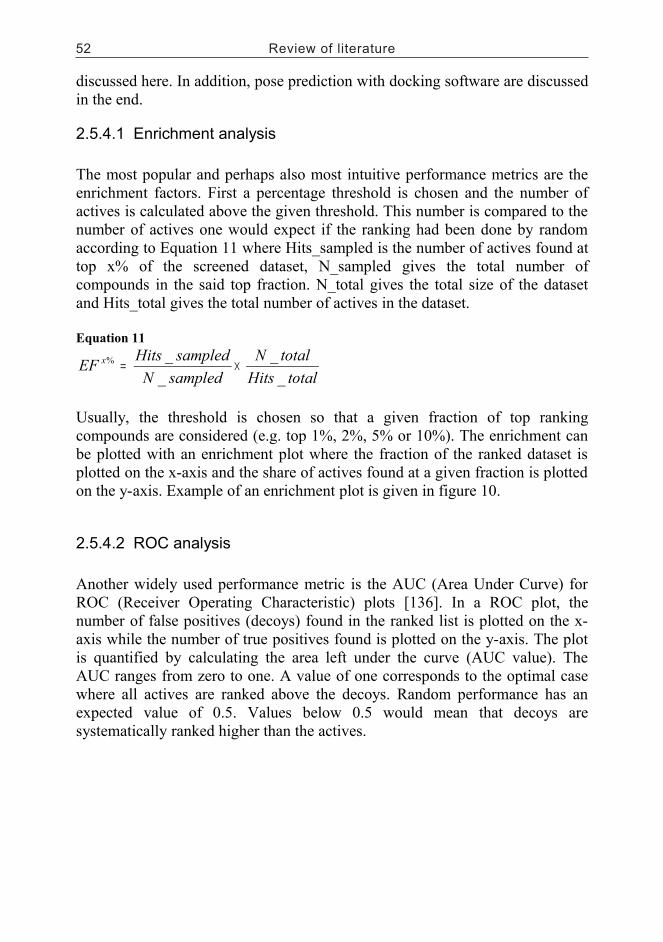
52 Review of literature
discussed here. In addition, pose prediction with docking software are discussed in the end.
2.5.4.1 Enrichment analysis
The most popular and perhaps also most intuitive performance metrics are the enrichment factors. First a percentage threshold is chosen and the number of actives is calculated above the given threshold. This number is compared to the number of actives one would expect if the ranking had been done by random according to Equation 11 where Hits_sampled is the number of actives found at top x% of the screened dataset, N_sampled gives the total number of compounds in the said top fraction. N_total gives the total size of the dataset and Hits_total gives the total number of actives in the dataset.
Equation 11
totalHits
totalN
sampledN
sampledHitsEF x
_
_
_
_% ×=
Usually, the threshold is chosen so that a given fraction of top ranking compounds are considered (e.g. top 1%, 2%, 5% or 10%). The enrichment can be plotted with an enrichment plot where the fraction of the ranked dataset is plotted on the x-axis and the share of actives found at a given fraction is plotted on the y-axis. Example of an enrichment plot is given in figure 10.
2.5.4.2 ROC analysis
Another widely used performance metric is the AUC (Area Under Curve) for ROC (Receiver Operating Characteristic) plots [136]. In a ROC plot, the number of false positives (decoys) found in the ranked list is plotted on the x-axis while the number of true positives found is plotted on the y-axis. The plot is quantified by calculating the area left under the curve (AUC value). The AUC ranges from zero to one. A value of one corresponds to the optimal case where all actives are ranked above the decoys. Random performance has an expected value of 0.5. Values below 0.5 would mean that decoys are systematically ranked higher than the actives.
Figure 10. Example of an enrichment plot for one sample (dotted line). Solid black line denotes the optimal scenario where all actives have been ranked before any of the inactives. Finely dashed black line denotes the expected case if the order of compounds is random.
One advantage of ROC analysis over the enrichment analysis is its insensitivity to the active/decoy ratio [137]. Enrichment factors at a given cutoff tend to drop as the relative number of decoys drops whereas ROC AUC is insensitive to this. Another benefit of ROC analysis is that it takes both true and false positive rates explicitly into account whereas enrichment analysis considers only the former. Additionally, one can calculate confidence intervals for ROC AUCs giving them more statistical power.
One commonly raised criticism of ROC AUC values is the fact that they quantify the global performance [138]. A given AUC value can result from either good or poor early performance. One is usually only interested in the molecules in the very top of a ranked list, after all the purpose of virtual screening is to choose a subset of molecules for experimental testing. Jain [137] advocated the use of the true positive rate at a given early false positive rate

Review of literature 53
discussed here. In addition, pose prediction with docking software are discussed in the end.
2.5.4.1 Enrichment analysis
The most popular and perhaps also most intuitive performance metrics are the enrichment factors. First a percentage threshold is chosen and the number of actives is calculated above the given threshold. This number is compared to the number of actives one would expect if the ranking had been done by random according to Equation 11 where Hits_sampled is the number of actives found at top x% of the screened dataset, N_sampled gives the total number of compounds in the said top fraction. N_total gives the total size of the dataset and Hits_total gives the total number of actives in the dataset.
Equation 11
totalHits
totalN
sampledN
sampledHitsEF x
_
_
_
_% ×=
Usually, the threshold is chosen so that a given fraction of top ranking compounds are considered (e.g. top 1%, 2%, 5% or 10%). The enrichment can be plotted with an enrichment plot where the fraction of the ranked dataset is plotted on the x-axis and the share of actives found at a given fraction is plotted on the y-axis. Example of an enrichment plot is given in figure 10.
2.5.4.2 ROC analysis
Another widely used performance metric is the AUC (Area Under Curve) for ROC (Receiver Operating Characteristic) plots [136]. In a ROC plot, the number of false positives (decoys) found in the ranked list is plotted on the x-axis while the number of true positives found is plotted on the y-axis. The plot is quantified by calculating the area left under the curve (AUC value). The AUC ranges from zero to one. A value of one corresponds to the optimal case where all actives are ranked above the decoys. Random performance has an expected value of 0.5. Values below 0.5 would mean that decoys are systematically ranked higher than the actives.
Figure 10. Example of an enrichment plot for one sample (dotted line). Solid black line denotes the optimal scenario where all actives have been ranked before any of the inactives. Finely dashed black line denotes the expected case if the order of compounds is random.
One advantage of ROC analysis over the enrichment analysis is its insensitivity to the active/decoy ratio [137]. Enrichment factors at a given cutoff tend to drop as the relative number of decoys drops whereas ROC AUC is insensitive to this. Another benefit of ROC analysis is that it takes both true and false positive rates explicitly into account whereas enrichment analysis considers only the former. Additionally, one can calculate confidence intervals for ROC AUCs giving them more statistical power.
One commonly raised criticism of ROC AUC values is the fact that they quantify the global performance [138]. A given AUC value can result from either good or poor early performance. One is usually only interested in the molecules in the very top of a ranked list, after all the purpose of virtual screening is to choose a subset of molecules for experimental testing. Jain [137] advocated the use of the true positive rate at a given early false positive rate
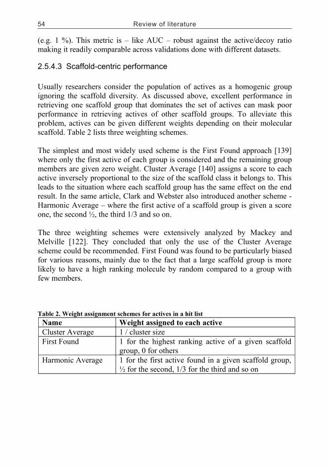
54 Review of literature
(e.g. 1 %). This metric is – like AUC – robust against the active/decoy ratio making it readily comparable across validations done with different datasets.
2.5.4.3 Scaffold-centric performance
Usually researchers consider the population of actives as a homogenic group ignoring the scaffold diversity. As discussed above, excellent performance in retrieving one scaffold group that dominates the set of actives can mask poor performance in retrieving actives of other scaffold groups. To alleviate this problem, actives can be given different weights depending on their molecular scaffold. Table 2 lists three weighting schemes.
The simplest and most widely used scheme is the First Found approach [139] where only the first active of each group is considered and the remaining group members are given zero weight. Cluster Average [140] assigns a score to each active inversely proportional to the size of the scaffold class it belongs to. This leads to the situation where each scaffold group has the same effect on the end result. In the same article, Clark and Webster also introduced another scheme - Harmonic Average – where the first active of a scaffold group is given a score one, the second ½, the third 1/3 and so on.
The three weighting schemes were extensively analyzed by Mackey and Melville [122]. They concluded that only the use of the Cluster Average scheme could be recommended. First Found was found to be particularly biased for various reasons, mainly due to the fact that a large scaffold group is more likely to have a high ranking molecule by random compared to a group with few members.
Table 2. Weight assignment schemes for actives in a hit list
Name Weight assigned to each active
Cluster Average 1 / cluster sizeFirst Found 1 for the highest ranking active of a given scaffold
group, 0 for others Harmonic Average 1 for the first active found in a given scaffold group,
½ for the second, 1/3 for the third and so on
2.5.4.4 Binding pose prediction
One additional performance metric important in validating docking performance still remains to be introduced. Pose prediction accuracy measures the fidelity how well docking software is able to reproduce the experimental ligand conformation. The industry standard for quantifying this is the RMSD (Root Mean Square Deviation) of non-hydrogen atoms of the computationally and experimentally derived binding poses (Equation 12).
Equation 12
n
xxRMSD
n
i ii∑ =−
= 1
2,2,1 )(
First, the co-crystallized ligand is removed from the protein active site and computationally derived conformers are derived for the ligand. Using the bioactive conformation from the crystal structure cannot be considered to represent the real-life situation where the bioactive conformation is rarely known. Therefore, pose prediction performance is also dependent on the ability of the conformer generation software to generate the bioactive conformation [141]. The objective is to have the highest-scoring pose within a given threshold from the experimental one. Generally, RMSD of 2 Å or better is considered sufficiently accurate to call the docking a success.
The steps given above describe cognate docking which should be considered as an upper limit to the performance of the docking protocol [137]. In cognate docking the protein conformation is optimal for the ligand to bind to and might not give a realistic picture of the performance if the protein can take various conformations upon ligand binding (i.e. induced fit). The protein conformation might not be suitable at all for discovery of actives of other scaffold classes which can lead to drastic changes in protein conformation. Therefore, cognate docking experiments should only be considered reliable if the target protein is known to be rigid and resistant to induced fit [137].
2.6 Data fusion
Data fusion (also called sensor fusion) means combining information retrieved from two or more sensors with the hope that the combined signal is better than the one retrieved from any of the individual sensors [142, 143]. In this case better can be that the signal is more reliable or more accurate, for example. Different kinds of sensors can be combined, each with its own strengths which

Review of literature 55
(e.g. 1 %). This metric is – like AUC – robust against the active/decoy ratio making it readily comparable across validations done with different datasets.
2.5.4.3 Scaffold-centric performance
Usually researchers consider the population of actives as a homogenic group ignoring the scaffold diversity. As discussed above, excellent performance in retrieving one scaffold group that dominates the set of actives can mask poor performance in retrieving actives of other scaffold groups. To alleviate this problem, actives can be given different weights depending on their molecular scaffold. Table 2 lists three weighting schemes.
The simplest and most widely used scheme is the First Found approach [139] where only the first active of each group is considered and the remaining group members are given zero weight. Cluster Average [140] assigns a score to each active inversely proportional to the size of the scaffold class it belongs to. This leads to the situation where each scaffold group has the same effect on the end result. In the same article, Clark and Webster also introduced another scheme - Harmonic Average – where the first active of a scaffold group is given a score one, the second ½, the third 1/3 and so on.
The three weighting schemes were extensively analyzed by Mackey and Melville [122]. They concluded that only the use of the Cluster Average scheme could be recommended. First Found was found to be particularly biased for various reasons, mainly due to the fact that a large scaffold group is more likely to have a high ranking molecule by random compared to a group with few members.
Table 2. Weight assignment schemes for actives in a hit list
Name Weight assigned to each active
Cluster Average 1 / cluster sizeFirst Found 1 for the highest ranking active of a given scaffold
group, 0 for others Harmonic Average 1 for the first active found in a given scaffold group,
½ for the second, 1/3 for the third and so on
2.5.4.4 Binding pose prediction
One additional performance metric important in validating docking performance still remains to be introduced. Pose prediction accuracy measures the fidelity how well docking software is able to reproduce the experimental ligand conformation. The industry standard for quantifying this is the RMSD (Root Mean Square Deviation) of non-hydrogen atoms of the computationally and experimentally derived binding poses (Equation 12).
Equation 12
n
xxRMSD
n
i ii∑ =−
= 1
2,2,1 )(
First, the co-crystallized ligand is removed from the protein active site and computationally derived conformers are derived for the ligand. Using the bioactive conformation from the crystal structure cannot be considered to represent the real-life situation where the bioactive conformation is rarely known. Therefore, pose prediction performance is also dependent on the ability of the conformer generation software to generate the bioactive conformation [141]. The objective is to have the highest-scoring pose within a given threshold from the experimental one. Generally, RMSD of 2 Å or better is considered sufficiently accurate to call the docking a success.
The steps given above describe cognate docking which should be considered as an upper limit to the performance of the docking protocol [137]. In cognate docking the protein conformation is optimal for the ligand to bind to and might not give a realistic picture of the performance if the protein can take various conformations upon ligand binding (i.e. induced fit). The protein conformation might not be suitable at all for discovery of actives of other scaffold classes which can lead to drastic changes in protein conformation. Therefore, cognate docking experiments should only be considered reliable if the target protein is known to be rigid and resistant to induced fit [137].
2.6 Data fusion
Data fusion (also called sensor fusion) means combining information retrieved from two or more sensors with the hope that the combined signal is better than the one retrieved from any of the individual sensors [142, 143]. In this case better can be that the signal is more reliable or more accurate, for example. Different kinds of sensors can be combined, each with its own strengths which

56 Review of literature
compensate weaknesses of the other sensors. Originally used for military uses such as target identification, it has now found use in a number of fields.
In drug discovery, data fusion has found applications in both ligand- and structure-based virtual screening [144]. More specifically, the first step is to rank a set of compounds with a number of virtual screening tools. Once the lists have been derived, they are combined into one fused list. MIN and SUM rules are commonly used for merging ranked lists of compounds. Using the MIN rule the value of a compound in the fused list equals to its smallest (minimum) rank in any of the lists being combined. Using the SUM rule the value of the compound in the fused list equals to the sum of ranks across all the lists being merged. Finally the compounds in the fused list are re-ranked based on their value.
2.6.1 Data fusion in ligand-based virtual screening
One way to perform data fusion in ligand-based virtual screening is to combine hit lists derived with more than one tool or similarity metric (similarity fusion). The other approach involves using only one tool but several template molecules (group fusion) [145].
2.6.1.1 Similarity fusion
In a study of similarity fusion using the SUM rule by Whittle et al. [146] they found that combining different similarity metrics generally improves results but this is not consistent across all test cases. Another important finding which applies to all types of data fusion is that the performance gained by combining data from different sources drops after inclusion of three or four rankings [147]. The effect has also been found in Publication I of this thesis. Salim et al. [148] did a comparison of similarity metrics. They observed that while a given metrics combination might perform well with one target class, it did not do so in another group. This has been largely attributed to different preferences similarity metrics have for the molecule size with some performing better with large molecules and others with small ones [74].
2.6.1.2 Group fusion
Whittle et al. [149] and Hert et al. [150] both studied the performance of group fusion. With similarity fusion, ranked lists must be fused using ranks as different methods/metrics have differing scales and distributions. This leads to the loss of information as the actual similarity scores are ignored. This is not a problem in
group fusion where fused lists can be generated with the similarity scores. Both Whittle et al. and Hert et al. found this approach to be superior to using ranks. In the former of the two studies, it was also found that group fusion performs well when the actives are structurally diverse.
2.6.1.3 Turbo similarity searching
Group fusion is not a viable option if only one known active exists. For this case, a data fusion methods known as turbo similarity searching (TSS) can be applied [151, 152]. The authors coined the method in analogy to a turbo booster in an engine that uses exhaust gases to increase the power of the engine. According to the similarity principle [68], the more similar a molecule is to the active template the higher the probability it is active as well. The authors of the TSS method take this principle a step further by assuming that the nearest neighbours in fact are active and that they can be used as templates as well. First the database is ranked by decreasing similarity to the active. The top scoring molecules are then used as templates which results in a ranked list for each nearest neighbour. Finally all the resulting lists are merged for a final fused list. The authors noticed this to lead to an improved performance despite the underlying assumption of the nearest neighbour being active, does not always hold true.
2.6.1.4 Work of Muchmore et al.
The data fusion techniques described above are simple but effective. One thing they do not indicate is the probability that a given compound will be effective. In work done by Muchmore et al. [153] chemical similarity (10 metrics) for a set of compound pairs was related to the experimental affinity data measured against 23 different protein targets for the same molecules. In the end, the authors could assign a probability as a function of their chemical similarity for two molecules being active against the same target.
These results are already useful when deciding objectively which compounds to select for experimental testing. The authors took the work still further by combining probabilities (or beliefs as they call it) of two or more similarity metrics. For this they employed Hooper’s rule (Equation 13) for combining evidence.
Equation 13
)1)(1(1 21int BBBjo −−−=

Review of literature 57
compensate weaknesses of the other sensors. Originally used for military uses such as target identification, it has now found use in a number of fields.
In drug discovery, data fusion has found applications in both ligand- and structure-based virtual screening [144]. More specifically, the first step is to rank a set of compounds with a number of virtual screening tools. Once the lists have been derived, they are combined into one fused list. MIN and SUM rules are commonly used for merging ranked lists of compounds. Using the MIN rule the value of a compound in the fused list equals to its smallest (minimum) rank in any of the lists being combined. Using the SUM rule the value of the compound in the fused list equals to the sum of ranks across all the lists being merged. Finally the compounds in the fused list are re-ranked based on their value.
2.6.1 Data fusion in ligand-based virtual screening
One way to perform data fusion in ligand-based virtual screening is to combine hit lists derived with more than one tool or similarity metric (similarity fusion). The other approach involves using only one tool but several template molecules (group fusion) [145].
2.6.1.1 Similarity fusion
In a study of similarity fusion using the SUM rule by Whittle et al. [146] they found that combining different similarity metrics generally improves results but this is not consistent across all test cases. Another important finding which applies to all types of data fusion is that the performance gained by combining data from different sources drops after inclusion of three or four rankings [147]. The effect has also been found in Publication I of this thesis. Salim et al. [148] did a comparison of similarity metrics. They observed that while a given metrics combination might perform well with one target class, it did not do so in another group. This has been largely attributed to different preferences similarity metrics have for the molecule size with some performing better with large molecules and others with small ones [74].
2.6.1.2 Group fusion
Whittle et al. [149] and Hert et al. [150] both studied the performance of group fusion. With similarity fusion, ranked lists must be fused using ranks as different methods/metrics have differing scales and distributions. This leads to the loss of information as the actual similarity scores are ignored. This is not a problem in
group fusion where fused lists can be generated with the similarity scores. Both Whittle et al. and Hert et al. found this approach to be superior to using ranks. In the former of the two studies, it was also found that group fusion performs well when the actives are structurally diverse.
2.6.1.3 Turbo similarity searching
Group fusion is not a viable option if only one known active exists. For this case, a data fusion methods known as turbo similarity searching (TSS) can be applied [151, 152]. The authors coined the method in analogy to a turbo booster in an engine that uses exhaust gases to increase the power of the engine. According to the similarity principle [68], the more similar a molecule is to the active template the higher the probability it is active as well. The authors of the TSS method take this principle a step further by assuming that the nearest neighbours in fact are active and that they can be used as templates as well. First the database is ranked by decreasing similarity to the active. The top scoring molecules are then used as templates which results in a ranked list for each nearest neighbour. Finally all the resulting lists are merged for a final fused list. The authors noticed this to lead to an improved performance despite the underlying assumption of the nearest neighbour being active, does not always hold true.
2.6.1.4 Work of Muchmore et al.
The data fusion techniques described above are simple but effective. One thing they do not indicate is the probability that a given compound will be effective. In work done by Muchmore et al. [153] chemical similarity (10 metrics) for a set of compound pairs was related to the experimental affinity data measured against 23 different protein targets for the same molecules. In the end, the authors could assign a probability as a function of their chemical similarity for two molecules being active against the same target.
These results are already useful when deciding objectively which compounds to select for experimental testing. The authors took the work still further by combining probabilities (or beliefs as they call it) of two or more similarity metrics. For this they employed Hooper’s rule (Equation 13) for combining evidence.
Equation 13
)1)(1(1 21int BBBjo −−−=

58 Review of literature
In this equation B1 is the belief associated with the chemical similarity value of the first metric and B2 is the belief for the second metric. Belief for the best performing individual metric ECFP_6 [71] was combined with beliefs for the other nine metrics. It was observed that the greatest improvement occurred when ECFP_6 and ROCS [87] were combined. This was logical as the two metrics measure similarity in different ways and whose similarity values correlate only slightly. Still a third belief from the remaining metrics was combined with ECFP_6 and ROCS. Combining the results from Daylight fingerprints [154] still led to slight improvement but adding a fourth metric did not lead to any further improvement.
The findings above were evaluated against an external test set of 134 active compounds from 28 target classes. The compound pairs arising from the same class were considered as active pairs while all the other pairs as inactive. Performances of the individual methods and the joint belief of ECFP_6, ROCS and Daylight in enriching the active pairs were assessed. For comparison, ranks from lists for ECFP_6, ROCS and Daylight were combined with the MAX, MIN and SUM rules and performances were assessed also for these fused lists. The joint belief fared better than any of the individual metrics as expected. MAX and MIN rules fared poorly when compared to ECFP_6 individually and the joint belief. However, the SUM rule gave similar performance to the joint belief. The authors noted that the belief theory should still be considered superior as it gives a quantitative probability for two molecules sharing activity against a target. This information is lost when using ranks as with the SUM rule.
As an additional note, the idea of assigning a probability for the biological similarity as function of chemical similarity was used in Publication I as well. Also the results and conclusions drawn were similar to those of Muchmore et al.
2.6.2 Data fusion in structure-based virtual screening
In structure-based virtual screening – or docking – data fusion is generally called consensus scoring [155, 156]. Here a molecule is first docked into the binding site using one scoring function and the resulting binding poses re-scored with one or more different scoring functions. These lists can then be merged using the same principles as with LBVS (Ligand-Based Virtual Screening) tools resulting in a fused list [157]. The scores calculated with the function used for docking can be used as well or ignored when making the final fused list . As with data fusion in LBVS, it is a good idea to combine scoring functions that make uncorrelated errors. Also scoring functions performing poorly individually should be ignored altogether as they will only deteriorate
the performance of those functions with good performance [157, 158]. Consensus scoring does not automatically lead to superior results. This was noted by Yang et al. [158] who concluded that consensus scoring does not always reach the performance of the best individual function but should be better than the average of the merged functions.
Care should also be taken when choosing which scoring function to use for the actual docking (the pose prediction) and which one for re-scoring. Studies by O’Boyle et al. and Cheng et al. [157, 159] both show that some functions are good in predicting the correct binding conformer while others are better in scoring the docked poses (i.e. giving better enrichment of actives over inactives). In the former of the two studies, the authors found that first docking the ligands with GOLD’s Chemscore function and re-ranking the compounds with Goldscore was superior to either of the individual functions. If the order of functions was changed, performance dropped significantly, being worse than with using Goldscore alone. The same was observed in the case that the scores of Chemscore were included in making the final ranking.
Review of literature 59
In this equation B1 is the belief associated with the chemical similarity value of the first metric and B2 is the belief for the second metric. Belief for the best performing individual metric ECFP_6 [71] was combined with beliefs for the other nine metrics. It was observed that the greatest improvement occurred when ECFP_6 and ROCS [87] were combined. This was logical as the two metrics measure similarity in different ways and whose similarity values correlate only slightly. Still a third belief from the remaining metrics was combined with ECFP_6 and ROCS. Combining the results from Daylight fingerprints [154] still led to slight improvement but adding a fourth metric did not lead to any further improvement.
The findings above were evaluated against an external test set of 134 active compounds from 28 target classes. The compound pairs arising from the same class were considered as active pairs while all the other pairs as inactive. Performances of the individual methods and the joint belief of ECFP_6, ROCS and Daylight in enriching the active pairs were assessed. For comparison, ranks from lists for ECFP_6, ROCS and Daylight were combined with the MAX, MIN and SUM rules and performances were assessed also for these fused lists. The joint belief fared better than any of the individual metrics as expected. MAX and MIN rules fared poorly when compared to ECFP_6 individually and the joint belief. However, the SUM rule gave similar performance to the joint belief. The authors noted that the belief theory should still be considered superior as it gives a quantitative probability for two molecules sharing activity against a target. This information is lost when using ranks as with the SUM rule.
As an additional note, the idea of assigning a probability for the biological similarity as function of chemical similarity was used in Publication I as well. Also the results and conclusions drawn were similar to those of Muchmore et al.
2.6.2 Data fusion in structure-based virtual screening
In structure-based virtual screening – or docking – data fusion is generally called consensus scoring [155, 156]. Here a molecule is first docked into the binding site using one scoring function and the resulting binding poses re-scored with one or more different scoring functions. These lists can then be merged using the same principles as with LBVS (Ligand-Based Virtual Screening) tools resulting in a fused list [157]. The scores calculated with the function used for docking can be used as well or ignored when making the final fused list . As with data fusion in LBVS, it is a good idea to combine scoring functions that make uncorrelated errors. Also scoring functions performing poorly individually should be ignored altogether as they will only deteriorate
the performance of those functions with good performance [157, 158]. Consensus scoring does not automatically lead to superior results. This was noted by Yang et al. [158] who concluded that consensus scoring does not always reach the performance of the best individual function but should be better than the average of the merged functions.
Care should also be taken when choosing which scoring function to use for the actual docking (the pose prediction) and which one for re-scoring. Studies by O’Boyle et al. and Cheng et al. [157, 159] both show that some functions are good in predicting the correct binding conformer while others are better in scoring the docked poses (i.e. giving better enrichment of actives over inactives). In the former of the two studies, the authors found that first docking the ligands with GOLD’s Chemscore function and re-ranking the compounds with Goldscore was superior to either of the individual functions. If the order of functions was changed, performance dropped significantly, being worse than with using Goldscore alone. The same was observed in the case that the scores of Chemscore were included in making the final ranking.
60 Aims of the study
3 Aims of the study
1. Relate chemical similarity scores given by a variety of ligand-based virtual screening tools to the biological similarity of small molecules. The goal was to have a conversion or look-up table that transforms an abstract chemical similarity score into a concrete probability value for two molecules having the same biological action.
2. Study the effect of combining results from several chemical similarity scores and the use of several template molecules.
3. Compare performance of ligand-based virtual screening tools in retrieving actives from a carefully designed benchmark ligand set. Additionally determine the applicability of these datasets for benchmarking.
4. Related to the third aim, study the performance of the virtual screening tools in performing scaffold-hopping, i.e. identifying two small molecules representing different chemotypes as similar.
4 Materials and methods
4.1 Datasets
4.1.1 Maximum Unbiased Validation (II, III)
MUV [133] contains validated active and inactive decoy molecules for 17 target classes (Publication II, table 1). Each target class has 30 actives and 15,000 decoys. Ligand 2D structures were downloaded from the MUV website [160].
4.1.2 Directory of Useful Decoys (I, III)
Directory of Useful Decoys (DUD) [123] contains 40 target classes with 11 to 444 active ligands per group. Each active molecule has 36 property-matched decoy molecules. Ligand structures were downloaded from the DUD web site [161].
4.1.3 NCI-60 (I, III)
Developmental Therapeutics Program (DTP) of the National Cancer Institute (NCI) [162] has over the years screened tens of thousands of small molecules for their ability to inhibit growth of cancer cells. The cancer cell lines with the most screening information available are jointly known as the NCI-60 cell lines. Datasets containing both the cytotoxicity data expressed as GI50 values (compound concentration that halves cancer cell growth rate) and the small molecule structures were downloaded from the DTP website [162].
4.2 Small molecule structures
4.2.1 Pre-treatment (I, II, III)
In Publication I, downloaded small molecule structures were used as they were except that any salts included in the structures were removed. For Publications II and III, the molecular structures, charges and bonds were standardized and all but the largest fragment in the structure record (i.e. the molecule itself) were removed using the Standardize Molecule tool of Pipeline Pilot. Additionally any duplicate entries were removed based on their Canonical SMILES strings.

Materials and methods 61
3 Aims of the study
1. Relate chemical similarity scores given by a variety of ligand-based virtual screening tools to the biological similarity of small molecules. The goal was to have a conversion or look-up table that transforms an abstract chemical similarity score into a concrete probability value for two molecules having the same biological action.
2. Study the effect of combining results from several chemical similarity scores and the use of several template molecules.
3. Compare performance of ligand-based virtual screening tools in retrieving actives from a carefully designed benchmark ligand set. Additionally determine the applicability of these datasets for benchmarking.
4. Related to the third aim, study the performance of the virtual screening tools in performing scaffold-hopping, i.e. identifying two small molecules representing different chemotypes as similar.
4 Materials and methods
4.1 Datasets
4.1.1 Maximum Unbiased Validation (II, III)
MUV [133] contains validated active and inactive decoy molecules for 17 target classes (Publication II, table 1). Each target class has 30 actives and 15,000 decoys. Ligand 2D structures were downloaded from the MUV website [160].
4.1.2 Directory of Useful Decoys (I, III)
Directory of Useful Decoys (DUD) [123] contains 40 target classes with 11 to 444 active ligands per group. Each active molecule has 36 property-matched decoy molecules. Ligand structures were downloaded from the DUD web site [161].
4.1.3 NCI-60 (I, III)
Developmental Therapeutics Program (DTP) of the National Cancer Institute (NCI) [162] has over the years screened tens of thousands of small molecules for their ability to inhibit growth of cancer cells. The cancer cell lines with the most screening information available are jointly known as the NCI-60 cell lines. Datasets containing both the cytotoxicity data expressed as GI50 values (compound concentration that halves cancer cell growth rate) and the small molecule structures were downloaded from the DTP website [162].
4.2 Small molecule structures
4.2.1 Pre-treatment (I, II, III)
In Publication I, downloaded small molecule structures were used as they were except that any salts included in the structures were removed. For Publications II and III, the molecular structures, charges and bonds were standardized and all but the largest fragment in the structure record (i.e. the molecule itself) were removed using the Standardize Molecule tool of Pipeline Pilot. Additionally any duplicate entries were removed based on their Canonical SMILES strings.

62 Materials and methods
4.2.2 3D conformations (I, II, III)
In Publication I, 3D structures were generated with Corina version 3.2 [33, 163]. For each 2D structure given as input, the program generated a multi-conformer library where energies of all conformers were within 20 kcal/mol of the minimum energy conformer. Separate sets of conformers were also generated for each stereoisomer of a molecule. The conformers were directly given as input for Almond [164] to calculate GRIND descriptors [165].
For BRUTUS calculations [81, 82], only the conformer with the minimum energy was retained for each stereoisomer. These were then further minimized with a custom made Sybyl script using the MMFF94s force field together with MMFF94 point charges [55]. These were used as templates in the BRUTUS search. Multi-conformer database files were generated using a systematic search functionality of Sybyl [166].
In Publications II and III, stereoisomers were first generated using the flipper tool part of the OpenEye software package [167] which generates the isomers only if stereoisomerism is not defined for a double bond or a chiral carbon. All 3D conformers were generated using OMEGA2 [45] with default settings. Afterwards, MMFF94 point charges [55] were calculated for each conformer using the molcharge tool from OpenEye [168]. For each stereoisomer the minimum energy conformer was used as a template. All the three 3D overlay tools in Publication II and III used exactly the same molecule files for both templates and database molecules.
4.3 Ligand-based virtual screening tools
4.3.1 UNITY fingerprints (I)
Tanimoto similarity of Unity fingerprints [169] were calculated with the Molecule Spreadsheet tool which is part of the Sybyl 8.0 modeling software [166]. The similarity scores were calculated for 38,332,428 molecule pairs representing 15,653 individual molecules from the NCI-60 dataset.
4.3.2 Daylight fingerprints (I)
Tanimoto similarity scores for Daylight fingerprints [154] of the NCI-60 dataset were kindly donated by Anders Wallqvist (Biotechnology HPC Software Applications Institute, Fort Detrick, MD, USA)
4.3.3 ECFP4/FCFP4 fingerprints (II)
ECFP4 and FCFP4 fingerprints were first generated for all ligands in the MUV dataset [133]. Pairwise Tanimoto similarities were then calculated within each of the 17 ligand sets. This was all done using Pipeline Pilot Student Edition [72].
4.3.4 GRIND descriptors (I)
GRid-INdependent descriptors (GRIND) describes the molecular interaction fields surrounding a molecule as a vector of values [165]. Each value represents a distance between two points in space around the molecule. The value in the bin is the largest product of interaction energies for interaction field nodes whose mutual distance falls into the distance bin.
GRIND descriptors were calculated for each conformer of the molecules in the NCI-60 dataset by using Almond 3.3.0 software [164]. First the molecular interaction fields were calculated with three probe types representing important non-covalent interaction types: DRY (hydrophobic interactions), O (hydrogen bond acceptor) and N1 (hydrogen bond donor). The fourth probe type (TIP) [170] was also used to describe the shape of the molecules. Ten correlograms (four auto-correlograms and six cross-correlograms) were generated each with 122 descriptors (distance bins).
The correlograms were exported into a text-file and concatenated into a single vector. The Pearson correlation coefficient was calculated between all GRIND descriptors of conformers of the molecules being compared. The largest coefficient value for any combination of conformers was used to represent similarity of the two molecules. This was done for 48,868,066 pairs representing 14,720 distinct molecules from the NCI-60 dataset.
4.3.5 BRUTUS (I, II, III)
For each template molecule, overlay against the multi-conformer database molecules was repeated using each stereoisomer. The stereoisomer conformer with the lowest energy was always used. The highest total score out of all stereoisomers was used to represent the similarity of the template molecule to the database molecules.
Version 0.8.7 of the BRUTUS software was used [81, 82]. Filtering of the results was switched off using the command line parameter (-f disable), and no overlays were retained during the screening to save hard disk space. Otherwise default parameters were used.
Materials and methods 63
4.2.2 3D conformations (I, II, III)
In Publication I, 3D structures were generated with Corina version 3.2 [33, 163]. For each 2D structure given as input, the program generated a multi-conformer library where energies of all conformers were within 20 kcal/mol of the minimum energy conformer. Separate sets of conformers were also generated for each stereoisomer of a molecule. The conformers were directly given as input for Almond [164] to calculate GRIND descriptors [165].
For BRUTUS calculations [81, 82], only the conformer with the minimum energy was retained for each stereoisomer. These were then further minimized with a custom made Sybyl script using the MMFF94s force field together with MMFF94 point charges [55]. These were used as templates in the BRUTUS search. Multi-conformer database files were generated using a systematic search functionality of Sybyl [166].
In Publications II and III, stereoisomers were first generated using the flipper tool part of the OpenEye software package [167] which generates the isomers only if stereoisomerism is not defined for a double bond or a chiral carbon. All 3D conformers were generated using OMEGA2 [45] with default settings. Afterwards, MMFF94 point charges [55] were calculated for each conformer using the molcharge tool from OpenEye [168]. For each stereoisomer the minimum energy conformer was used as a template. All the three 3D overlay tools in Publication II and III used exactly the same molecule files for both templates and database molecules.
4.3 Ligand-based virtual screening tools
4.3.1 UNITY fingerprints (I)
Tanimoto similarity of Unity fingerprints [169] were calculated with the Molecule Spreadsheet tool which is part of the Sybyl 8.0 modeling software [166]. The similarity scores were calculated for 38,332,428 molecule pairs representing 15,653 individual molecules from the NCI-60 dataset.
4.3.2 Daylight fingerprints (I)
Tanimoto similarity scores for Daylight fingerprints [154] of the NCI-60 dataset were kindly donated by Anders Wallqvist (Biotechnology HPC Software Applications Institute, Fort Detrick, MD, USA)
4.3.3 ECFP4/FCFP4 fingerprints (II)
ECFP4 and FCFP4 fingerprints were first generated for all ligands in the MUV dataset [133]. Pairwise Tanimoto similarities were then calculated within each of the 17 ligand sets. This was all done using Pipeline Pilot Student Edition [72].
4.3.4 GRIND descriptors (I)
GRid-INdependent descriptors (GRIND) describes the molecular interaction fields surrounding a molecule as a vector of values [165]. Each value represents a distance between two points in space around the molecule. The value in the bin is the largest product of interaction energies for interaction field nodes whose mutual distance falls into the distance bin.
GRIND descriptors were calculated for each conformer of the molecules in the NCI-60 dataset by using Almond 3.3.0 software [164]. First the molecular interaction fields were calculated with three probe types representing important non-covalent interaction types: DRY (hydrophobic interactions), O (hydrogen bond acceptor) and N1 (hydrogen bond donor). The fourth probe type (TIP) [170] was also used to describe the shape of the molecules. Ten correlograms (four auto-correlograms and six cross-correlograms) were generated each with 122 descriptors (distance bins).
The correlograms were exported into a text-file and concatenated into a single vector. The Pearson correlation coefficient was calculated between all GRIND descriptors of conformers of the molecules being compared. The largest coefficient value for any combination of conformers was used to represent similarity of the two molecules. This was done for 48,868,066 pairs representing 14,720 distinct molecules from the NCI-60 dataset.
4.3.5 BRUTUS (I, II, III)
For each template molecule, overlay against the multi-conformer database molecules was repeated using each stereoisomer. The stereoisomer conformer with the lowest energy was always used. The highest total score out of all stereoisomers was used to represent the similarity of the template molecule to the database molecules.
Version 0.8.7 of the BRUTUS software was used [81, 82]. Filtering of the results was switched off using the command line parameter (-f disable), and no overlays were retained during the screening to save hard disk space. Otherwise default parameters were used.

64 Materials and methods
In publication I, BRUTUS total scores were calculated for 3,018,315 molecule pairs representing 12,767 distinct molecules.
4.3.6 ROCS and EON (II, III)
The same template and database molecule conformations as with BRUTUS were given as an input for ROCS version 2.3.1 [87] as well. The highest ROCS total score (shape score plus colorscore) found was used to represent similarity of a pair of molecules. The top scoring ROCS overlays were re-scored with EON version 2.0.1 [171] which evaluates similarity based on the electrostatic complementarity. The total score given by EON was used (shape score plus the Poisson-Boltzmann electrostatic Tanimoto coefficient) for each molecule pair.
4.4 Relating chemical and biological similarity of small molecules
4.4.1 Definition of biological similarity (I, III)
In Publication I, biological similarity values for the molecules in the NCI-60 set were donated by Anders Wallqvist who had done the calculations for their article [172]. They had first log-transformed the GI50 data and then filtered out molecules with data missing for more than 20 cell lines. Furthermore, only molecules with a signal variation of 0.02 or greater were retained. From here on, the vector of log-transformed GI50 values is referred as the cytotoxicity profile of the molecule.
Biological similarity of two molecules was defined as the Pearson correlation of cytotoxicity profiles of the molecules. Cell lines with missing values for either of the molecules were ignored.
In Publication III, the August 2008 version of the NCI-60 screening data [162] was used. Here the purpose was not to study the relationship between chemical and biological similarity domains per se but rather to transform the different chemical similarity scores into probability values describing the probability of them being biologically similar. In effect, this converted the chemical similarity scores into a common reference framework enabling their direct comparison.
The data handling was different from that done by Wallqvist et al [172]. First the GI50 values were transformed into their negative logarithms (pGI50). Molecules with missing data on 20 cell lines or more and those being inactive (pGI50 < 5) in five cell lines or more were removed. Additionally molecules for which no structures were available or for which 3D conformer could not be
generated were ignored from further analysis. After this 9,542 high quality molecules remained to be used in the study.
The pGI50 values were re-scaled by assigning a value of zero to data points where pGI50 < 5 or if the value was missing. Those data points where pGI50 >8 were set to 3. The remaining values were re-scaled from 0 to 3. Biological similarity was calculated using the continuous Tanimoto formula (Equation 14).
Equation 14
∑∑∑∑
−+=
i
ii
i
ii
i
ii
i
ii
bababbaa
ba
biosimil***
*
,
where biosimila,b is the biological similarity of molecules a and b, ai and bi
denote the re-scaled pGI50 value of cell line i for molecules a and b, respectively.
4.4.2 Relating chemical and biological similarity scores (I, III)
In both Publications I and III the chemical and biological similarity values were related in the same way. First the following definition was made:
Equation 15
);( bracN ≥≥
which defines the number of compound pairs with a chemical similarity of a or greater and biological similarity of b or greater.
This leads to definition of the ratio in Equation 16.
Equation 16
)_;(
);()|(
minsimilbiolracN
bracNbracF
≥≥≥≥≡==
where the Equation 15 is used as the numerator. The denominator is the total number of molecule pairs with a chemical similarity of a or greater. The term biol_similmin refers to the minimum biological similarity value two molecules can have. In Publication I, biol_similmin = -1 and in Publication III biol_similmin
= 0.

Materials and methods 65
In publication I, BRUTUS total scores were calculated for 3,018,315 molecule pairs representing 12,767 distinct molecules.
4.3.6 ROCS and EON (II, III)
The same template and database molecule conformations as with BRUTUS were given as an input for ROCS version 2.3.1 [87] as well. The highest ROCS total score (shape score plus colorscore) found was used to represent similarity of a pair of molecules. The top scoring ROCS overlays were re-scored with EON version 2.0.1 [171] which evaluates similarity based on the electrostatic complementarity. The total score given by EON was used (shape score plus the Poisson-Boltzmann electrostatic Tanimoto coefficient) for each molecule pair.
4.4 Relating chemical and biological similarity of small molecules
4.4.1 Definition of biological similarity (I, III)
In Publication I, biological similarity values for the molecules in the NCI-60 set were donated by Anders Wallqvist who had done the calculations for their article [172]. They had first log-transformed the GI50 data and then filtered out molecules with data missing for more than 20 cell lines. Furthermore, only molecules with a signal variation of 0.02 or greater were retained. From here on, the vector of log-transformed GI50 values is referred as the cytotoxicity profile of the molecule.
Biological similarity of two molecules was defined as the Pearson correlation of cytotoxicity profiles of the molecules. Cell lines with missing values for either of the molecules were ignored.
In Publication III, the August 2008 version of the NCI-60 screening data [162] was used. Here the purpose was not to study the relationship between chemical and biological similarity domains per se but rather to transform the different chemical similarity scores into probability values describing the probability of them being biologically similar. In effect, this converted the chemical similarity scores into a common reference framework enabling their direct comparison.
The data handling was different from that done by Wallqvist et al [172]. First the GI50 values were transformed into their negative logarithms (pGI50). Molecules with missing data on 20 cell lines or more and those being inactive (pGI50 < 5) in five cell lines or more were removed. Additionally molecules for which no structures were available or for which 3D conformer could not be
generated were ignored from further analysis. After this 9,542 high quality molecules remained to be used in the study.
The pGI50 values were re-scaled by assigning a value of zero to data points where pGI50 < 5 or if the value was missing. Those data points where pGI50 >8 were set to 3. The remaining values were re-scaled from 0 to 3. Biological similarity was calculated using the continuous Tanimoto formula (Equation 14).
Equation 14
∑∑∑∑
−+=
i
ii
i
ii
i
ii
i
ii
bababbaa
ba
biosimil***
*
,
where biosimila,b is the biological similarity of molecules a and b, ai and bi
denote the re-scaled pGI50 value of cell line i for molecules a and b, respectively.
4.4.2 Relating chemical and biological similarity scores (I, III)
In both Publications I and III the chemical and biological similarity values were related in the same way. First the following definition was made:
Equation 15
);( bracN ≥≥
which defines the number of compound pairs with a chemical similarity of a or greater and biological similarity of b or greater.
This leads to definition of the ratio in Equation 16.
Equation 16
)_;(
);()|(
minsimilbiolracN
bracNbracF
≥≥≥≥≡==
where the Equation 15 is used as the numerator. The denominator is the total number of molecule pairs with a chemical similarity of a or greater. The term biol_similmin refers to the minimum biological similarity value two molecules can have. In Publication I, biol_similmin = -1 and in Publication III biol_similmin
= 0.

66 Materials and methods
In Publication I, Equation 16 was used to generate look-up tables for the different chemical similarity scores at the following thresholds for biological similarity b: 0.4, 0.5, 0.6, 0.7, 0.8 and 0.9. In Publication III, only the value of b = 0.5 was used. If a value in a look-up table was based on less than hundred molecule pairs, it was replaced with the ratio for the highest chemical similarity value that was based on at least 100 pairs. This was done to prevent the random fluctuation with small sample values from distorting the results. In Publication I these look-up tables were also generated for combinations of chemical similarity scores to allow the quantitative study of data fusion and synergy.
In Publication I, Equation 17 was defined as well. Equation 17
);_(
);()|(
min brsimilchemcN
bracNbracG
≥≥≥≥≡==
where chem_similmin refers to the smallest chemical similarity score possible for the virtual screening tool used. With the Equation, “inverse” look-up tables were generated that give the ratio of molecule pairs with a chemical similarity of a or greater for all molecule pairs with a biological similarity of b or greater.
4.4.3 Synergy calculation (I)
One of the main goals of the thesis was to study synergy [144] arising from combining results of two or more virtual screening tools. The following equation gives the definition of relative synergy.
Equation 18
[ ])|min_,();|,min_(max
)|,()|,(
brchemyixFbrjychemxF
brjyixFbrjyixS
yx
rel =========≡===
where function F is as defined in Equation 17, chem_minx and chem._miny are the smallest similarity scores possible with tools x and y, respectively. Analogously absolute synergy is defined as the numerator subtracted from the denominator of Equation 18.
4.5 Performance metrics
In the three Publications, various performance metrics were used to quantify the capability of the tools for enriching active molecules and performing scaffold hopping. All the scores were calculated with in-house Perl and SQL scripts.
4.5.1 Enrichment of actives (I, II)
Enrichment factors were calculated using Equation 11. Enrichment was evaluated at the top 1, 2, 5, and 10 % of the ranked list in Publication I while in Publication II also the enrichment at the top 20% was calculated.
In addition to the enrichment factors, also the Area Under Curve (AUC) of the Receiver Operating Characteristics (ROC) was used. A ROC curve describes the share of actives found (true positive rate) as function of inactives found (false positive rate) at a given position of a ranked list. If all actives have been ranked before any of the inactives, the ROC value is one. The expected value of the ROC AUC is 0.5 if the actives are randomly distributed.
4.5.2 Scaffold hopping performance (III)
The ability of a ligand-based virtual screening tool in identifying actives with different chemotypes as chemically similar was quantified on the ligand set level with Equation 19.
Equation 19
[ ]2
min,,,
,
)__(*)_1(
n
similchemsimilchemsimilscaff
scoreji
toolji
a
ji
settool
∑≠
−−=
where the numerator iterates through all molecule pairs in the ligand set and sums up their scaffold weighted chemical similarities. Chemical similarity scores used were estimated by using biological similarity scores taken from look-up tables generated with Equation 17. The more similar the scaffolds of a molecule pair are the less weight their chemical similarity is given. This effect is further augmented with exponent a. Term chem_similmin, tool is the smallest estimated biological similarity score in the look-up table of a given tool. This
parameter value was slightly over 0.08 for all methods. Its purpose is to diminish the impact of insignificant similarity scores. The sum is divided by the number of molecule pairs (n2) to allow comparison between ligand sets.

Materials and methods 67
In Publication I, Equation 16 was used to generate look-up tables for the different chemical similarity scores at the following thresholds for biological similarity b: 0.4, 0.5, 0.6, 0.7, 0.8 and 0.9. In Publication III, only the value of b = 0.5 was used. If a value in a look-up table was based on less than hundred molecule pairs, it was replaced with the ratio for the highest chemical similarity value that was based on at least 100 pairs. This was done to prevent the random fluctuation with small sample values from distorting the results. In Publication I these look-up tables were also generated for combinations of chemical similarity scores to allow the quantitative study of data fusion and synergy.
In Publication I, Equation 17 was defined as well. Equation 17
);_(
);()|(
min brsimilchemcN
bracNbracG
≥≥≥≥≡==
where chem_similmin refers to the smallest chemical similarity score possible for the virtual screening tool used. With the Equation, “inverse” look-up tables were generated that give the ratio of molecule pairs with a chemical similarity of a or greater for all molecule pairs with a biological similarity of b or greater.
4.4.3 Synergy calculation (I)
One of the main goals of the thesis was to study synergy [144] arising from combining results of two or more virtual screening tools. The following equation gives the definition of relative synergy.
Equation 18
[ ])|min_,();|,min_(max
)|,()|,(
brchemyixFbrjychemxF
brjyixFbrjyixS
yx
rel =========≡===
where function F is as defined in Equation 17, chem_minx and chem._miny are the smallest similarity scores possible with tools x and y, respectively. Analogously absolute synergy is defined as the numerator subtracted from the denominator of Equation 18.
4.5 Performance metrics
In the three Publications, various performance metrics were used to quantify the capability of the tools for enriching active molecules and performing scaffold hopping. All the scores were calculated with in-house Perl and SQL scripts.
4.5.1 Enrichment of actives (I, II)
Enrichment factors were calculated using Equation 11. Enrichment was evaluated at the top 1, 2, 5, and 10 % of the ranked list in Publication I while in Publication II also the enrichment at the top 20% was calculated.
In addition to the enrichment factors, also the Area Under Curve (AUC) of the Receiver Operating Characteristics (ROC) was used. A ROC curve describes the share of actives found (true positive rate) as function of inactives found (false positive rate) at a given position of a ranked list. If all actives have been ranked before any of the inactives, the ROC value is one. The expected value of the ROC AUC is 0.5 if the actives are randomly distributed.
4.5.2 Scaffold hopping performance (III)
The ability of a ligand-based virtual screening tool in identifying actives with different chemotypes as chemically similar was quantified on the ligand set level with Equation 19.
Equation 19
[ ]2
min,,,
,
)__(*)_1(
n
similchemsimilchemsimilscaff
scoreji
toolji
a
ji
settool
∑≠
−−=
where the numerator iterates through all molecule pairs in the ligand set and sums up their scaffold weighted chemical similarities. Chemical similarity scores used were estimated by using biological similarity scores taken from look-up tables generated with Equation 17. The more similar the scaffolds of a molecule pair are the less weight their chemical similarity is given. This effect is further augmented with exponent a. Term chem_similmin, tool is the smallest estimated biological similarity score in the look-up table of a given tool. This
parameter value was slightly over 0.08 for all methods. Its purpose is to diminish the impact of insignificant similarity scores. The sum is divided by the number of molecule pairs (n2) to allow comparison between ligand sets.

68 Materials and methods
4.6 Molecular scaffolds (III)
The scaffold of a small molecule was defined as its carbon skeleton, i.e. all heavy atoms were changed into carbons and all bonds were made single (see Figure 2 in Publication III). ECFP_4 fingerprints of the scaffolds were generated with Pipeline Pilot [72] and the scaffold similarity of two molecules was defined as the Tanimoto similarity (Table 1) of ECFP_4 fingerprints of their scaffolds [71].
4.7 Scaffold hopping analysis
4.7.1 Identification of scaffold hops (I)
To identify individual examples of scaffold hopping, molecule pairs from the NCI dataset were picked that fulfilled the following criteria. First they had to have a high biological similarity score (cytotoxicity profile correlation >= 0.50) indicating a common mode of action and possibly the same binding target. Additionally the pairs had to have a high score with both 3D tools (GRIND score >= 0.90 and BRUTUS total score >= 2.8) and a low score with the two fingerprint tools (both Daylight and Unity Tanimoto <= 0.40).
It was also interesting to analyze biologically similar molecule pairs (cytotoxicity profile correlation >= 0.50) that were structurally similar (both Daylight and Unity Tanimoto >= 0.70) but which the two 3D tools failed to identify as similar (Brutus total score <= 2.2 and GRIND score <= 0.850).
4.7.2 Scaffold hopping heatmaps (III)
Scaffold hopping patterns within a ligand set were visualized using heatmaps with the molecules hierarchically clustered along the vertical and hierarchical axes of the heatmap. The heatmaps were generated using the statistical software R [173].
Major components of a heatmap are shown in Figure 5 of Publication III and they are as follows. (1) The heatmap itself, identical dendrograms with the ligand set members clustered according to their scaffolds, (2) template molecules are on the vertical axis and (3) the database molecules on the horizontal axis. All dendrograms were generated using average linkage. Chemical similarity of two molecules can be read from their intersection on the heatmap. (4) Color Key describes the correspondence between color intensity on the heatmap and the quantitative similarity score.
4.8 Similarity and group fusion
In the thesis, both similarity and group fusion were applied. The former refers to combining results from two or more virtual screening tools while the latter refers to combining results from several template molecules.
4.8.1 Similarity fusion (I, II)
In publication I, similarity fusion was applied to the DUD dataset [123]. The chemical similarity of all actives was calculated with all other actives and decoys in the ligand set of the template using two tools, GRIND [165] and BRUTUS [81, 82]. The two sets of hit lists were merged using both the traditional SUM and MAX rules and the look-up tables generated using Equation 17 modified for use with two or more tools. The latter fusion technique is referred to as “biofusion” here on for clarity.
For MAX and SUM similarity fusions, the GRIND and BRUTUS scores were first re-scaled from 0 to 1 using Equation 20
Equation 20
min_max_ chemchem
aarescaled −
=
where a is the original score, chem_max is the maximum score given by the method (one for GRIND, four for BRUTUS) and chem_min is the minimum score given by the method (-1 for GRIND and 0 for BRUTUS).
Using the MAX rule, the larger score of the re-scaled scores was used to represent a molecule pair in the fused hit list. With the SUM rule the sum of the two rescaled scores was used. Lastly, the fused lists were re-ranked in the descending order.
With biofusion, first the correct row was identified using the two similarity scores and the probability for biological similarity was read and used to represent the molecule pair in the fused list. Finally the fused lists were re-ranked in the descending order.
In Publication I, the MAX and SUM rules were applied to re-scaled similarity scores – not ranks of the molecules. For the thesis, the GRIND and Brutus results were also fused based on ranks of the molecules by using the MIN and SUM rules as described below for Publication II.

Materials and methods 69
4.6 Molecular scaffolds (III)
The scaffold of a small molecule was defined as its carbon skeleton, i.e. all heavy atoms were changed into carbons and all bonds were made single (see Figure 2 in Publication III). ECFP_4 fingerprints of the scaffolds were generated with Pipeline Pilot [72] and the scaffold similarity of two molecules was defined as the Tanimoto similarity (Table 1) of ECFP_4 fingerprints of their scaffolds [71].
4.7 Scaffold hopping analysis
4.7.1 Identification of scaffold hops (I)
To identify individual examples of scaffold hopping, molecule pairs from the NCI dataset were picked that fulfilled the following criteria. First they had to have a high biological similarity score (cytotoxicity profile correlation >= 0.50) indicating a common mode of action and possibly the same binding target. Additionally the pairs had to have a high score with both 3D tools (GRIND score >= 0.90 and BRUTUS total score >= 2.8) and a low score with the two fingerprint tools (both Daylight and Unity Tanimoto <= 0.40).
It was also interesting to analyze biologically similar molecule pairs (cytotoxicity profile correlation >= 0.50) that were structurally similar (both Daylight and Unity Tanimoto >= 0.70) but which the two 3D tools failed to identify as similar (Brutus total score <= 2.2 and GRIND score <= 0.850).
4.7.2 Scaffold hopping heatmaps (III)
Scaffold hopping patterns within a ligand set were visualized using heatmaps with the molecules hierarchically clustered along the vertical and hierarchical axes of the heatmap. The heatmaps were generated using the statistical software R [173].
Major components of a heatmap are shown in Figure 5 of Publication III and they are as follows. (1) The heatmap itself, identical dendrograms with the ligand set members clustered according to their scaffolds, (2) template molecules are on the vertical axis and (3) the database molecules on the horizontal axis. All dendrograms were generated using average linkage. Chemical similarity of two molecules can be read from their intersection on the heatmap. (4) Color Key describes the correspondence between color intensity on the heatmap and the quantitative similarity score.
4.8 Similarity and group fusion
In the thesis, both similarity and group fusion were applied. The former refers to combining results from two or more virtual screening tools while the latter refers to combining results from several template molecules.
4.8.1 Similarity fusion (I, II)
In publication I, similarity fusion was applied to the DUD dataset [123]. The chemical similarity of all actives was calculated with all other actives and decoys in the ligand set of the template using two tools, GRIND [165] and BRUTUS [81, 82]. The two sets of hit lists were merged using both the traditional SUM and MAX rules and the look-up tables generated using Equation 17 modified for use with two or more tools. The latter fusion technique is referred to as “biofusion” here on for clarity.
For MAX and SUM similarity fusions, the GRIND and BRUTUS scores were first re-scaled from 0 to 1 using Equation 20
Equation 20
min_max_ chemchem
aarescaled −
=
where a is the original score, chem_max is the maximum score given by the method (one for GRIND, four for BRUTUS) and chem_min is the minimum score given by the method (-1 for GRIND and 0 for BRUTUS).
Using the MAX rule, the larger score of the re-scaled scores was used to represent a molecule pair in the fused hit list. With the SUM rule the sum of the two rescaled scores was used. Lastly, the fused lists were re-ranked in the descending order.
With biofusion, first the correct row was identified using the two similarity scores and the probability for biological similarity was read and used to represent the molecule pair in the fused list. Finally the fused lists were re-ranked in the descending order.
In Publication I, the MAX and SUM rules were applied to re-scaled similarity scores – not ranks of the molecules. For the thesis, the GRIND and Brutus results were also fused based on ranks of the molecules by using the MIN and SUM rules as described below for Publication II.

70 Materials and methods
In Publication II, the MIN (analogous to the MAX rule) and AVG (analogous to the SUM rule) were used. The major difference to Publication I was that the chemical similarity scores were not re-scaled but rather each molecule was represented by its rank in a single-method list. Similarity fusion was applied on five ligand-based virtual screening tools (FCFP_4, ECFP_4, BRUTUS, ROCS and EON) which had been first used to generate ranked lists of ligand sets in the MUV by using each active as the template molecule.For the MIN rule the smallest rank a molecule had in any of the five lists was used to represent the molecule in the final list and for the AVG rule the average of the five ranks was used. In the end, the fused lists were re-ranked in the ascending order.
4.8.2 Group fusion (II)
Use of multiple templates was studied in Publication II. Two approaches for picking the templates were tested: random and diversity-based. The size of the template sets ranged from two to ten molecules in the random picking strategy. For the diversity-based picking also a set size of one template was tested.
Within the random approach, hundred sets were randomly picked for each template set size from each of the 17 MUV ligand sets. This was done separately for each chemical similarity metric. In addition to single methods
also the fused lists generated with MIN and AVG rules were considered as chemical similarity metrics.
The Partitioning Around Medoids (PAM) algorithm [174] as implemented in the R software [173] was used for picking the diverse template sets. For input, a matrix of pair-wise active ligand distances was given for each target class. For each chemical similarity metric, one set of each size was chosen from each of the MUV ligandsets. As with the random picking strategy, the similarity fusion rank lists were considered as chemical similarity metrics.
Irrespective of the template picking strategy the hit lists of the templates in the set were fused in the same way. The largest similarity score a database molecule had to any of the templates in the set was used to represent the database molecule in the final list. For the similarity fusion metrics (which consisted of ranks) the smallest value was chosen to represent the database molecule.
4.9 Activity cliff analysis (II)
Since one of the possible reasons for the poor performance of a ligand-based virtual screening tool is activity cliffs, their frequency was evaluated. For this purpose, the screening results of 391 bioassays were downloaded from the NIH PubChem repository [134, 135].
Next all template-decoy pairs, where the decoy was in the top 1 percent of the hit list of the template, were listed. For each molecule pair, both the number of PubChem assays where both molecules had been tested and the number of assays where both molecules were found to be active were calculated.
Materials and methods 71
In Publication II, the MIN (analogous to the MAX rule) and AVG (analogous to the SUM rule) were used. The major difference to Publication I was that the chemical similarity scores were not re-scaled but rather each molecule was represented by its rank in a single-method list. Similarity fusion was applied on five ligand-based virtual screening tools (FCFP_4, ECFP_4, BRUTUS, ROCS and EON) which had been first used to generate ranked lists of ligand sets in the MUV by using each active as the template molecule.For the MIN rule the smallest rank a molecule had in any of the five lists was used to represent the molecule in the final list and for the AVG rule the average of the five ranks was used. In the end, the fused lists were re-ranked in the ascending order.
4.8.2 Group fusion (II)
Use of multiple templates was studied in Publication II. Two approaches for picking the templates were tested: random and diversity-based. The size of the template sets ranged from two to ten molecules in the random picking strategy. For the diversity-based picking also a set size of one template was tested.
Within the random approach, hundred sets were randomly picked for each template set size from each of the 17 MUV ligand sets. This was done separately for each chemical similarity metric. In addition to single methods
also the fused lists generated with MIN and AVG rules were considered as chemical similarity metrics.
The Partitioning Around Medoids (PAM) algorithm [174] as implemented in the R software [173] was used for picking the diverse template sets. For input, a matrix of pair-wise active ligand distances was given for each target class. For each chemical similarity metric, one set of each size was chosen from each of the MUV ligandsets. As with the random picking strategy, the similarity fusion rank lists were considered as chemical similarity metrics.
Irrespective of the template picking strategy the hit lists of the templates in the set were fused in the same way. The largest similarity score a database molecule had to any of the templates in the set was used to represent the database molecule in the final list. For the similarity fusion metrics (which consisted of ranks) the smallest value was chosen to represent the database molecule.
4.9 Activity cliff analysis (II)
Since one of the possible reasons for the poor performance of a ligand-based virtual screening tool is activity cliffs, their frequency was evaluated. For this purpose, the screening results of 391 bioassays were downloaded from the NIH PubChem repository [134, 135].
Next all template-decoy pairs, where the decoy was in the top 1 percent of the hit list of the template, were listed. For each molecule pair, both the number of PubChem assays where both molecules had been tested and the number of assays where both molecules were found to be active were calculated.

72 Results and discussion
5 Results and discussion
5.1 Relationship between chemical and biological similarity (I)
5.1.1 Single methods
In respect to enrichment of biologically similar molecule pairs (cytotoxicity profile correlation of 0.8 or greater), the fingerprints Daylight and UNITY fingerprints performed best while GRIND and BRUTUS performed markedly worse (Figure 2 in Publication I).
One of the reasons for the inferior performance of the two 3D methods lies in the fact that many (18.2 %) of biologically similar molecule pairs share the same scaffold. Pairs such as these are easily identified as similar by using fingerprints. 3D methods require conformers of the molecules and if the conformer generator fails to re-produce the biological conformer, two molecules are incorrectly identified as dissimilar.
Another important thing to note in Figure 2 (Publication I) is that the line for none of the methods approaches unity. One reason is the inherent fuzziness of the cytotoxicity data as the same phenotype (the cell growth inhibition in this case) can be due to different mechanisms. Therefore two molecules with a high biological similarity score can bind into completely different targets with no chemical similarity identifiable with any method. Conversely two non-identical molecules can be identified as completely similar by a similarity tool if the feature differentiating the two molecules is missed by the tool. This feature can be important for biological activity leading to a false positive.
Biological similarity of the NCI molecules was also used to enrich chemically similar compounds (Figure 3 in Publication I). When the biological similarity was 0.6 or greater enrichment could be observed.
5.1.2 Combinations of methods
Interesting findings were made when the share of biologically active pairs was analyzed as a function of two or more methods. In Figure 11 the share of biologically similar compound pairs as a function of Brutus total score and Tanimoto similarity of Unity fingerprints is illustrated. Contours show Brutus/Unity similarity score combinations where the share of biologically similar pairs is 0.03, 0.06 and 0.09. An important observation is the curvature of
the contours. This is a sign of synergy for the combinations of similarity scores intersecting at the curved area.
Point 1 in Figure 11 is in the intersection of Brutus total score of 2.36 and Unity similarity of 0.50. The share of biologically similar pairs at this point is 0.03. More formally this can be expressed using Equation 17: F(brutus = 2.36, Unity = 0.50 | r = 0.80) = 0.03. Taking only the Brutus score in account (Point 2 on Figure 11) we get only F(brutus = 2.36, Unity = 0.00 | r = 0.80) = 0.002 while taking only the Unity similarity in account (Point 3 on Figure 11) gives us F(brutus = 0.00, Unity = 0.50 | r = 0.80) = 0.011. Having these three ratios we can use Equation 18 to calculate the relative synergy at point 1 as 0.03 / max{0.002; 0.011} = 2.7.
Relative synergies for different combinations of Brutus and Unity similarities are plotted in Figure 12. Evidently the largest gains from combining the two methods are achieved when only relatively high similarity scores are combined, i.e. when Brutus total score is between two and three and Unity Tanimoto is between 0.3 and 0.7. If one similarity metric is already very high the additional information from another method does not lead to further gain.
Figure 5 in Publication I plots maximal relative synergies for different combinations of the four methods studied in the paper. Two main conclusions can be drawn. First, synergy gains drop dramatically once the third or the fourth method is added into the combination. Two methods are able to describe chemical properties of the molecules to such an extent that the third and fourth method do effect only slightly. The second important finding is that combining two methods with the same underlying principle does not lead to much benefit.
This is clear with the combination of Daylight and Unity fingerprints which both describe the molecule by iterating bond paths.
When Publication II was being finalized another paper by Muchmore et al. [153] was published where the same idea for relating chemical and biological similarity domains was presented. The results obtained and the conclusions drawn by the authors are very similar to those presented here.

Results and discussion 73
5 Results and discussion
5.1 Relationship between chemical and biological similarity (I)
5.1.1 Single methods
In respect to enrichment of biologically similar molecule pairs (cytotoxicity profile correlation of 0.8 or greater), the fingerprints Daylight and UNITY fingerprints performed best while GRIND and BRUTUS performed markedly worse (Figure 2 in Publication I).
One of the reasons for the inferior performance of the two 3D methods lies in the fact that many (18.2 %) of biologically similar molecule pairs share the same scaffold. Pairs such as these are easily identified as similar by using fingerprints. 3D methods require conformers of the molecules and if the conformer generator fails to re-produce the biological conformer, two molecules are incorrectly identified as dissimilar.
Another important thing to note in Figure 2 (Publication I) is that the line for none of the methods approaches unity. One reason is the inherent fuzziness of the cytotoxicity data as the same phenotype (the cell growth inhibition in this case) can be due to different mechanisms. Therefore two molecules with a high biological similarity score can bind into completely different targets with no chemical similarity identifiable with any method. Conversely two non-identical molecules can be identified as completely similar by a similarity tool if the feature differentiating the two molecules is missed by the tool. This feature can be important for biological activity leading to a false positive.
Biological similarity of the NCI molecules was also used to enrich chemically similar compounds (Figure 3 in Publication I). When the biological similarity was 0.6 or greater enrichment could be observed.
5.1.2 Combinations of methods
Interesting findings were made when the share of biologically active pairs was analyzed as a function of two or more methods. In Figure 11 the share of biologically similar compound pairs as a function of Brutus total score and Tanimoto similarity of Unity fingerprints is illustrated. Contours show Brutus/Unity similarity score combinations where the share of biologically similar pairs is 0.03, 0.06 and 0.09. An important observation is the curvature of
the contours. This is a sign of synergy for the combinations of similarity scores intersecting at the curved area.
Point 1 in Figure 11 is in the intersection of Brutus total score of 2.36 and Unity similarity of 0.50. The share of biologically similar pairs at this point is 0.03. More formally this can be expressed using Equation 17: F(brutus = 2.36, Unity = 0.50 | r = 0.80) = 0.03. Taking only the Brutus score in account (Point 2 on Figure 11) we get only F(brutus = 2.36, Unity = 0.00 | r = 0.80) = 0.002 while taking only the Unity similarity in account (Point 3 on Figure 11) gives us F(brutus = 0.00, Unity = 0.50 | r = 0.80) = 0.011. Having these three ratios we can use Equation 18 to calculate the relative synergy at point 1 as 0.03 / max{0.002; 0.011} = 2.7.
Relative synergies for different combinations of Brutus and Unity similarities are plotted in Figure 12. Evidently the largest gains from combining the two methods are achieved when only relatively high similarity scores are combined, i.e. when Brutus total score is between two and three and Unity Tanimoto is between 0.3 and 0.7. If one similarity metric is already very high the additional information from another method does not lead to further gain.
Figure 5 in Publication I plots maximal relative synergies for different combinations of the four methods studied in the paper. Two main conclusions can be drawn. First, synergy gains drop dramatically once the third or the fourth method is added into the combination. Two methods are able to describe chemical properties of the molecules to such an extent that the third and fourth method do effect only slightly. The second important finding is that combining two methods with the same underlying principle does not lead to much benefit.
This is clear with the combination of Daylight and Unity fingerprints which both describe the molecule by iterating bond paths.
When Publication II was being finalized another paper by Muchmore et al. [153] was published where the same idea for relating chemical and biological similarity domains was presented. The results obtained and the conclusions drawn by the authors are very similar to those presented here.

74 Results and discussion
Figure 11. The share of biologically similar molecule pairs (cytotoxicity profile greater than or equal to 0.80) as function of Brutus total score and Tanimoto similarity of Unity fingerprints. See the text for detailed discussion.
Figure 12. Relative synergy for combinations of Brutus total score and Unity Tanimoto.
5.2 The enrichment of actives in the MUV dataset (II)
The enrichment of active molecules from a set of actives and decoys is the primary job of any virtual screening tool. When five individual ligand-based virtual screening tools (ECFP_4 and FCFP_4 fingerprints, EON, BRUTUS and ROCS) were evaluated against the MUV dataset the results were disappointing (Figure 2 of Publication II). Significant enrichment was observed only for four ligand sets (aid548, aid832, aid846 and aid852) out of seventeen. In the following three reasons for the poor performance are proposed and discussed. These are non-overlapping binding poses, false negatives and activity cliffs.
5.2.1 Non-overlapping binding poses
Different ligands can inhibit the same process in different ways. They can bind different sub-cavities of the same binding site or different binding sites or proteins altogether. In this case a method comparing ligands by their chemical properties cannot be expected to identify them as similar. Some ligand sets are based on cell-based reporter gene assays when the exact binding partner of the ligand is unclear [175]. It is noteworthy that these five ligand sets are among those where the enrichment of actives is disappointing (aid466, aid600, aid692, aid858 and aid859).
This is a quality control issue that should be taken into account better in future. The best but also the most costly way to handle this is to crystallize the ligands together with their targets or to perform competitive assays using ligands with a known binding mode.
5.2.2 False negatives
Some of the decoy molecules are very similar to the actives of the same ligand set. The possibility increases that these are in fact false negatives and therefore the poor enrichment values are partially due to misclassified decoys. All decoys had been found to be inactive in the high throughput screening results deposited at the PubChem assay database. Unlike actives found in the screens, the inactives were not validated in a secondary screen. The authors of the MUVdataset had made a small-scale literature search with the top ranking decoys and they found no evidence for their activity [133].
When future versions of benchmark datasets are designed it would be very useful to have some of the decoys experimentally validated. As this is slow and
Results and discussion 75
Figure 11. The share of biologically similar molecule pairs (cytotoxicity profile greater than or equal to 0.80) as function of Brutus total score and Tanimoto similarity of Unity fingerprints. See the text for detailed discussion.
Figure 12. Relative synergy for combinations of Brutus total score and Unity Tanimoto.
5.2 The enrichment of actives in the MUV dataset (II)
The enrichment of active molecules from a set of actives and decoys is the primary job of any virtual screening tool. When five individual ligand-based virtual screening tools (ECFP_4 and FCFP_4 fingerprints, EON, BRUTUS and ROCS) were evaluated against the MUV dataset the results were disappointing (Figure 2 of Publication II). Significant enrichment was observed only for four ligand sets (aid548, aid832, aid846 and aid852) out of seventeen. In the following three reasons for the poor performance are proposed and discussed. These are non-overlapping binding poses, false negatives and activity cliffs.
5.2.1 Non-overlapping binding poses
Different ligands can inhibit the same process in different ways. They can bind different sub-cavities of the same binding site or different binding sites or proteins altogether. In this case a method comparing ligands by their chemical properties cannot be expected to identify them as similar. Some ligand sets are based on cell-based reporter gene assays when the exact binding partner of the ligand is unclear [175]. It is noteworthy that these five ligand sets are among those where the enrichment of actives is disappointing (aid466, aid600, aid692, aid858 and aid859).
This is a quality control issue that should be taken into account better in future. The best but also the most costly way to handle this is to crystallize the ligands together with their targets or to perform competitive assays using ligands with a known binding mode.
5.2.2 False negatives
Some of the decoy molecules are very similar to the actives of the same ligand set. The possibility increases that these are in fact false negatives and therefore the poor enrichment values are partially due to misclassified decoys. All decoys had been found to be inactive in the high throughput screening results deposited at the PubChem assay database. Unlike actives found in the screens, the inactives were not validated in a secondary screen. The authors of the MUVdataset had made a small-scale literature search with the top ranking decoys and they found no evidence for their activity [133].
When future versions of benchmark datasets are designed it would be very useful to have some of the decoys experimentally validated. As this is slow and

76 Results and discussion
costly, it might be realistic to test only a small set of decoys but this would still be a step forwards.
5.2.3 Activity cliffs
Activity cliffs [176, 177] are defined as small changes in structure of the molecule that induce major changes in the binding affinity. They could be the reason why some of the decoys in the MUV resemble actives while not being false negatives.
Figures 6 and 7 in Publication II show results of the activity cliff analysis performed on top-ranking decoys. The closer a decoy molecule is to the template molecule the greater the probability that there is at least one PubChem assay (against another target) where both the decoy and the template have been confirmed as active. For example, compound CID 2883004 (Figure 8 in Publication II) is a validated Rho-Kinase 2 inhibitor from the MUV ligand set aid644. Compound CID 1506381 (Figure 8 in Publication II) is an inactive decoy from the same set but structurally very similar to CID 2883004. It is possible that the bulky side group of the decoy induces steric clash with the kinase and inactivity. However both molecules are active in three confirmatory screens found in PubChem: aid825 (Cathepsin L inhibition assay), aid830 (Cathepsin B inhibition assay) and aid938 (Thyroid Stimulating Hormone Receptor agonist assay). One can hypothesize that the bulky side group of CID 1506381 is better accommodated by these three targets.
It needs to be noted that these activity cliffs are still only putative as long as a confirmatory assay is not done to rule out the possibility of the decoy being a false negative.
5.3 The effect of data fusion on the enrichment of actives
Both the similarity fusion (use of two or more virtual screening tools) and the group fusion (use of two or more template molecules) were studied in the thesis.
5.3.1 Similarity fusion (I, II)
In publication I, three different similarity fusion techniques were applied to combining GRIND and Brutus hit lists from the DUD dataset and compared to each other and the two screening tools. These were MAX (“MAX rescaled”) and SUM (“SUM rescaled”) rules applied on re-scaled similarity scores and the look-up tables generated using Equation 17 (“biofusion”). Results from the two
tools were also fused using MIN (“minrank”) and SUM (“sumrank”) rules on molecule ranks.
Figure 13a illustrates the distribution of enrichment factors for both the individual methods and the different data fusion techniques on the level of a single template meaning that each distribution is based on 2,805 observations. It is evident that all data fusion methods lead to improved enrichment compared to using either GRIND or Brutus alone. Out of the traditional data fusion techniques, “SUM re-scaled” scores has the highest median enrichment. Interestingly, the biofusion gives the best overall enrichment. The enrichment factor distribution is shown in the Figure 13a for six thresholds for the biological similarity (Bio, r=0.4 to 0.9). Judging from the results in Figure 13a there is a little difference in which threshold to be used for the biological similarity.
Figure 13b also displays the distribution of enrichment factors – this time averaged across the 40 ligandsets in the DUD. Here the difference between the biofusion and the best traditional data fusion technique (minrank) is practically zero. This figure also gives a more realistic picture of the relative performance of these techniques as the Figure 13a is biased by the superior performance of the biofusion in some ligand sets with large number of templates such as the cox2 set with 343 actives. As the scaffold diversity of actives in the DUD is rather low [132] enrichment experiments done with structurally very similar template molecules produces only a little new knowledge.
Equivalent performance of the biofusion with the minrank can initially lead to a conclusion that the added complexity of the biofusion makes it an inferior approach. However, it has one advantage over any of the more simple data fusion approaches: interpretativeness. Ranks given by the minrank, for instance have no meaning themselves outside their context. In contrast, the value given by the biofusion as a function of similarity scores gives an intuitive and very useful variable: the probability that the two molecules produce a similar biological phenotype. This could, for example be used for choosing objectively which molecules from a virtual screen to choose for the experimental testing.
In publication II, only the rank fusion rules AVG and MIN were used in combining results from the five ligand-based virtual screening tools used in the study. The results of this are shown in Figures 1 and 2 of Publication II. Both fusion rules are among the top performers when the average enrichment factors within ligand sets are considered although an individual tool can still outperform both data fusion methods (Figure 2 of Publication II). However, the data fusion is no miracle maker if none of the tools being fused performs well.

Results and discussion 77
costly, it might be realistic to test only a small set of decoys but this would still be a step forwards.
5.2.3 Activity cliffs
Activity cliffs [176, 177] are defined as small changes in structure of the molecule that induce major changes in the binding affinity. They could be the reason why some of the decoys in the MUV resemble actives while not being false negatives.
Figures 6 and 7 in Publication II show results of the activity cliff analysis performed on top-ranking decoys. The closer a decoy molecule is to the template molecule the greater the probability that there is at least one PubChem assay (against another target) where both the decoy and the template have been confirmed as active. For example, compound CID 2883004 (Figure 8 in Publication II) is a validated Rho-Kinase 2 inhibitor from the MUV ligand set aid644. Compound CID 1506381 (Figure 8 in Publication II) is an inactive decoy from the same set but structurally very similar to CID 2883004. It is possible that the bulky side group of the decoy induces steric clash with the kinase and inactivity. However both molecules are active in three confirmatory screens found in PubChem: aid825 (Cathepsin L inhibition assay), aid830 (Cathepsin B inhibition assay) and aid938 (Thyroid Stimulating Hormone Receptor agonist assay). One can hypothesize that the bulky side group of CID 1506381 is better accommodated by these three targets.
It needs to be noted that these activity cliffs are still only putative as long as a confirmatory assay is not done to rule out the possibility of the decoy being a false negative.
5.3 The effect of data fusion on the enrichment of actives
Both the similarity fusion (use of two or more virtual screening tools) and the group fusion (use of two or more template molecules) were studied in the thesis.
5.3.1 Similarity fusion (I, II)
In publication I, three different similarity fusion techniques were applied to combining GRIND and Brutus hit lists from the DUD dataset and compared to each other and the two screening tools. These were MAX (“MAX rescaled”) and SUM (“SUM rescaled”) rules applied on re-scaled similarity scores and the look-up tables generated using Equation 17 (“biofusion”). Results from the two
tools were also fused using MIN (“minrank”) and SUM (“sumrank”) rules on molecule ranks.
Figure 13a illustrates the distribution of enrichment factors for both the individual methods and the different data fusion techniques on the level of a single template meaning that each distribution is based on 2,805 observations. It is evident that all data fusion methods lead to improved enrichment compared to using either GRIND or Brutus alone. Out of the traditional data fusion techniques, “SUM re-scaled” scores has the highest median enrichment. Interestingly, the biofusion gives the best overall enrichment. The enrichment factor distribution is shown in the Figure 13a for six thresholds for the biological similarity (Bio, r=0.4 to 0.9). Judging from the results in Figure 13a there is a little difference in which threshold to be used for the biological similarity.
Figure 13b also displays the distribution of enrichment factors – this time averaged across the 40 ligandsets in the DUD. Here the difference between the biofusion and the best traditional data fusion technique (minrank) is practically zero. This figure also gives a more realistic picture of the relative performance of these techniques as the Figure 13a is biased by the superior performance of the biofusion in some ligand sets with large number of templates such as the cox2 set with 343 actives. As the scaffold diversity of actives in the DUD is rather low [132] enrichment experiments done with structurally very similar template molecules produces only a little new knowledge.
Equivalent performance of the biofusion with the minrank can initially lead to a conclusion that the added complexity of the biofusion makes it an inferior approach. However, it has one advantage over any of the more simple data fusion approaches: interpretativeness. Ranks given by the minrank, for instance have no meaning themselves outside their context. In contrast, the value given by the biofusion as a function of similarity scores gives an intuitive and very useful variable: the probability that the two molecules produce a similar biological phenotype. This could, for example be used for choosing objectively which molecules from a virtual screen to choose for the experimental testing.
In publication II, only the rank fusion rules AVG and MIN were used in combining results from the five ligand-based virtual screening tools used in the study. The results of this are shown in Figures 1 and 2 of Publication II. Both fusion rules are among the top performers when the average enrichment factors within ligand sets are considered although an individual tool can still outperform both data fusion methods (Figure 2 of Publication II). However, the data fusion is no miracle maker if none of the tools being fused performs well.

78 Results and discussion
Figure 13. The distribution of enrichment factors at the top 1 percent of the ranked hitlist for BRUTUS and GRIND and the different data fusion techniques used. a) individual template molecules, b) average enrichment factors of the 40 ligand sets in the DUD
5.3.2 Group fusion (II)
Use of several templates in Publication II led to the improved enrichment as shown in the Figure 3 in Publication II. Additionally the more templates that were used the better the enrichment (Figure 5 in Publication II). This was hardly surprising since more of the chemical space is covered with several molecules as compared to using only a single molecule.
The template picking strategy also made a major difference to the enrichment. Figure 4 in Publication II shows the average enrichment across the 17 MUV ligand sets. Blue line illustrates the performance when five templates were chosen by random and the green line has the best enrichment for each ligand set with any of the 100 randomly picked template sets. The orange line shows the enrichment factors for the five-member template set picked based on diversity. For most ligand sets the enrichment factor for the diverse template set lies somewhere between the average random and the maximum random lines.
The superior performance of diversely picked templates over the random selection is hardly surprising as by definition a larger portion of the chemical space is covered than can be expected by using a single random set. It is however, noteworthy that the PAM algorithm used here does not yield optimal results as some of the randomly chosen template sets (green line in Figure 4, Publication II) outperform it. Therefore a topic of future work could be the testing of other (clustering) algorithms for choosing the template set.
In the real world scenario probably all available actives would be used as templates to maximize the chemical space screened and the diversity of any potential hits. Picking a diverse template set would therefore be done only if computational resources dictate an upper limit for the number of templates.
5.4 Scaffold hopping
5.4.1 Example pairs (I)
To understand better the screening tools used in Publication I, individual biologically similar molecule pairs were studied that were given high scores either exclusively by 3D tools (GRIND and BRUTUS) or exclusively by the fingerprints (Daylight and UNITY).
Figure 8 in Publication I shows a pair of molecules (NSC 639500 and NSC 657835) which is a good example of 3D tools identifying the chemical similarity despite of very different 2D structures of the molecules. The overlay of the two molecules in Figure 8b of Publication I illustrates the good steric
Results and discussion 79
Figure 13. The distribution of enrichment factors at the top 1 percent of the ranked hitlist for BRUTUS and GRIND and the different data fusion techniques used. a) individual template molecules, b) average enrichment factors of the 40 ligand sets in the DUD
5.3.2 Group fusion (II)
Use of several templates in Publication II led to the improved enrichment as shown in the Figure 3 in Publication II. Additionally the more templates that were used the better the enrichment (Figure 5 in Publication II). This was hardly surprising since more of the chemical space is covered with several molecules as compared to using only a single molecule.
The template picking strategy also made a major difference to the enrichment. Figure 4 in Publication II shows the average enrichment across the 17 MUV ligand sets. Blue line illustrates the performance when five templates were chosen by random and the green line has the best enrichment for each ligand set with any of the 100 randomly picked template sets. The orange line shows the enrichment factors for the five-member template set picked based on diversity. For most ligand sets the enrichment factor for the diverse template set lies somewhere between the average random and the maximum random lines.
The superior performance of diversely picked templates over the random selection is hardly surprising as by definition a larger portion of the chemical space is covered than can be expected by using a single random set. It is however, noteworthy that the PAM algorithm used here does not yield optimal results as some of the randomly chosen template sets (green line in Figure 4, Publication II) outperform it. Therefore a topic of future work could be the testing of other (clustering) algorithms for choosing the template set.
In the real world scenario probably all available actives would be used as templates to maximize the chemical space screened and the diversity of any potential hits. Picking a diverse template set would therefore be done only if computational resources dictate an upper limit for the number of templates.
5.4 Scaffold hopping
5.4.1 Example pairs (I)
To understand better the screening tools used in Publication I, individual biologically similar molecule pairs were studied that were given high scores either exclusively by 3D tools (GRIND and BRUTUS) or exclusively by the fingerprints (Daylight and UNITY).
Figure 8 in Publication I shows a pair of molecules (NSC 639500 and NSC 657835) which is a good example of 3D tools identifying the chemical similarity despite of very different 2D structures of the molecules. The overlay of the two molecules in Figure 8b of Publication I illustrates the good steric

80 Results and discussion
overlap of the molecules. Also the carbonyl groups are pointing roughly in the same direction.
Low fingerprint and high 3D similarity scores do not necessarily mean the two molecules would constitute a non-obvious case of scaffold hopping. This is exemplified by the Figure 9 of Publication I. To the human eye the structural similarity of molecules NSC 113764 and NSC 676181 is very obvious. Neither GRIND nor Brutus has any problems in scoring the pair as similar. Surprisingly both fingerprint methods fail in identifying them as similar. The substitution of a nitrogen atom in NSC 113764 with a carbon in NSC 676181 and the fourth ring in the latter molecule are enough to confuse the fingerprints.
5.4.2 Scaffold heatmaps (III)
The visualization of the heatmap scores as calculated with Equation 19 (a = 3) are shown in Figure 14 for both the MUV and the DUD datasets. Within both datasets the ligand sets can be divided into three major clusters based on their heatmap score profiles across ROCS, EON and BRUTUS. Cluster 1 contains ligand sets with high scores for either of the two 3D overlay tools scoring similarity of electrostatic fields (BRUTUS and EON). Heatmap scores for ligand sets in Cluster 3 are clearly lower for all overlay tools. For the MUV sets in this cluster, only EON is giving reasonable scores. Lastly, all methods give low scores for ligand sets in Cluster 2.
Of particular interest is the markedly inferior performance of ROCS compared to EON and BRUTUS in almost all of the ligand sets. Exceptions to this are ligand sets er_agonist, ar and comt of the DUD. Especially for the COMT (Catechol O-methyltransferase ligands) set only ROCS is giving a reasonable score. Using the heatmaps in Figure 8a-c of Publication III, it is easy to identify to which molecule pairs ROCS is giving high scores while EON and BRUTUS fail to do so. For example, when molecule ZINC00392003 is used as a template, ROCS gives high scores for a set of five molecules falling into a different dendrogram based on their scaffolds (solid lined box in Figure 8a of Publication III). Inspecting these pairs in a more detail gives us important knowledge of the overlay tools used.
For example, the ROCS total score is 1.776 for pair ZINC00392003 and ZINC03814484 when the former is used as the template (Figure 15a and Figure 8d-e of Publication III). Particularly the colorscore (measuring the overlap of pharmacophoric features) is almost perfect (0.9770) although the nitro group of ZINC03814484 is not matched with an isofunctional group in the template. ROCS is only concerned with matching the functional groups of the template
molecule and not of the database molecule. The same holds true for other database molecules boxed in Figure 8a of Publication III which all can be overlaid in a way matching the hydroxyl and the carbonyl of the template but whose additional functional groups do not have to be matched.
If the template molecule (ZINC00392003) is modified by adding a hydroxyl group and overlay re-scored (Figure 15b), the total score drops to 1.409 with the color score going down to 0.652 since the added group in the template is not matched by the other molecule.
This scoring strategy is in stark contrast with EON and BRUTUS which require functional groups in both molecules to be matched. Therefore the lack of an isofunctional group overlapping the nitro group ZINC03814484 leads to a low similarity score.
Another interesting region in the ROCS heatmap for COMT (dashed box in Figure 8a in Publication III) is where ZINC00392003 is the database molecule and the five compounds in the Figure 8e of Publication III are used as templates. Here the similarity is very low owing to the fact that only some of functional groups in the templates are matched by ZINC00392003. This raises the issue of which molecule to use as a template when generating overlays of active molecules for a pharmacophore model, for example. If the “wrong” template is used there is a risk that the correct overlay of the molecules is missed. Therefore molecule pairs should be evaluated systematically by using each molecule as the template.
The scaffold definition (carbon skeletons) and the metric used to describe their similarity (ECFP_4 fingerprints) is one of many possible approaches. Each definition has its advantages and disadvantages and one problem with the approach taken here is illustrated by the ligand set GPB (Glycogen phosphorylase beta inhibitors) member of the DUD set. The ligand set has very high heatmap scores for all three tools evaluated (last row in Figure 14a). However, almost all ligands except three are built around the same ring (Figure 10d in Publication III) and one would expect such a ligand set to get a low score due to the term in Equation 19 disfavouring structurally similar pairs. The pairs are however, given surprisingly low scaffold similarity scores. This is attributable to the small size and the low complexity of the ligands when only a few bits are turned on in the fingerprint. Therefore just a different side group – for example – means that a relatively large number of fingerprint bits are in the different state. This is then reflected as a low Tanimoto similarity (Figure 10e in Publication III). If terminal side chains had been ignored this would not be the case. However, this might lead into new problems with other molecule pairs as exemplified with hypothetical molecules in Figure 3 and 4 of Publication III.

Results and discussion 81
overlap of the molecules. Also the carbonyl groups are pointing roughly in the same direction.
Low fingerprint and high 3D similarity scores do not necessarily mean the two molecules would constitute a non-obvious case of scaffold hopping. This is exemplified by the Figure 9 of Publication I. To the human eye the structural similarity of molecules NSC 113764 and NSC 676181 is very obvious. Neither GRIND nor Brutus has any problems in scoring the pair as similar. Surprisingly both fingerprint methods fail in identifying them as similar. The substitution of a nitrogen atom in NSC 113764 with a carbon in NSC 676181 and the fourth ring in the latter molecule are enough to confuse the fingerprints.
5.4.2 Scaffold heatmaps (III)
The visualization of the heatmap scores as calculated with Equation 19 (a = 3) are shown in Figure 14 for both the MUV and the DUD datasets. Within both datasets the ligand sets can be divided into three major clusters based on their heatmap score profiles across ROCS, EON and BRUTUS. Cluster 1 contains ligand sets with high scores for either of the two 3D overlay tools scoring similarity of electrostatic fields (BRUTUS and EON). Heatmap scores for ligand sets in Cluster 3 are clearly lower for all overlay tools. For the MUV sets in this cluster, only EON is giving reasonable scores. Lastly, all methods give low scores for ligand sets in Cluster 2.
Of particular interest is the markedly inferior performance of ROCS compared to EON and BRUTUS in almost all of the ligand sets. Exceptions to this are ligand sets er_agonist, ar and comt of the DUD. Especially for the COMT (Catechol O-methyltransferase ligands) set only ROCS is giving a reasonable score. Using the heatmaps in Figure 8a-c of Publication III, it is easy to identify to which molecule pairs ROCS is giving high scores while EON and BRUTUS fail to do so. For example, when molecule ZINC00392003 is used as a template, ROCS gives high scores for a set of five molecules falling into a different dendrogram based on their scaffolds (solid lined box in Figure 8a of Publication III). Inspecting these pairs in a more detail gives us important knowledge of the overlay tools used.
For example, the ROCS total score is 1.776 for pair ZINC00392003 and ZINC03814484 when the former is used as the template (Figure 15a and Figure 8d-e of Publication III). Particularly the colorscore (measuring the overlap of pharmacophoric features) is almost perfect (0.9770) although the nitro group of ZINC03814484 is not matched with an isofunctional group in the template. ROCS is only concerned with matching the functional groups of the template
molecule and not of the database molecule. The same holds true for other database molecules boxed in Figure 8a of Publication III which all can be overlaid in a way matching the hydroxyl and the carbonyl of the template but whose additional functional groups do not have to be matched.
If the template molecule (ZINC00392003) is modified by adding a hydroxyl group and overlay re-scored (Figure 15b), the total score drops to 1.409 with the color score going down to 0.652 since the added group in the template is not matched by the other molecule.
This scoring strategy is in stark contrast with EON and BRUTUS which require functional groups in both molecules to be matched. Therefore the lack of an isofunctional group overlapping the nitro group ZINC03814484 leads to a low similarity score.
Another interesting region in the ROCS heatmap for COMT (dashed box in Figure 8a in Publication III) is where ZINC00392003 is the database molecule and the five compounds in the Figure 8e of Publication III are used as templates. Here the similarity is very low owing to the fact that only some of functional groups in the templates are matched by ZINC00392003. This raises the issue of which molecule to use as a template when generating overlays of active molecules for a pharmacophore model, for example. If the “wrong” template is used there is a risk that the correct overlay of the molecules is missed. Therefore molecule pairs should be evaluated systematically by using each molecule as the template.
The scaffold definition (carbon skeletons) and the metric used to describe their similarity (ECFP_4 fingerprints) is one of many possible approaches. Each definition has its advantages and disadvantages and one problem with the approach taken here is illustrated by the ligand set GPB (Glycogen phosphorylase beta inhibitors) member of the DUD set. The ligand set has very high heatmap scores for all three tools evaluated (last row in Figure 14a). However, almost all ligands except three are built around the same ring (Figure 10d in Publication III) and one would expect such a ligand set to get a low score due to the term in Equation 19 disfavouring structurally similar pairs. The pairs are however, given surprisingly low scaffold similarity scores. This is attributable to the small size and the low complexity of the ligands when only a few bits are turned on in the fingerprint. Therefore just a different side group – for example – means that a relatively large number of fingerprint bits are in the different state. This is then reflected as a low Tanimoto similarity (Figure 10e in Publication III). If terminal side chains had been ignored this would not be the case. However, this might lead into new problems with other molecule pairs as exemplified with hypothetical molecules in Figure 3 and 4 of Publication III.
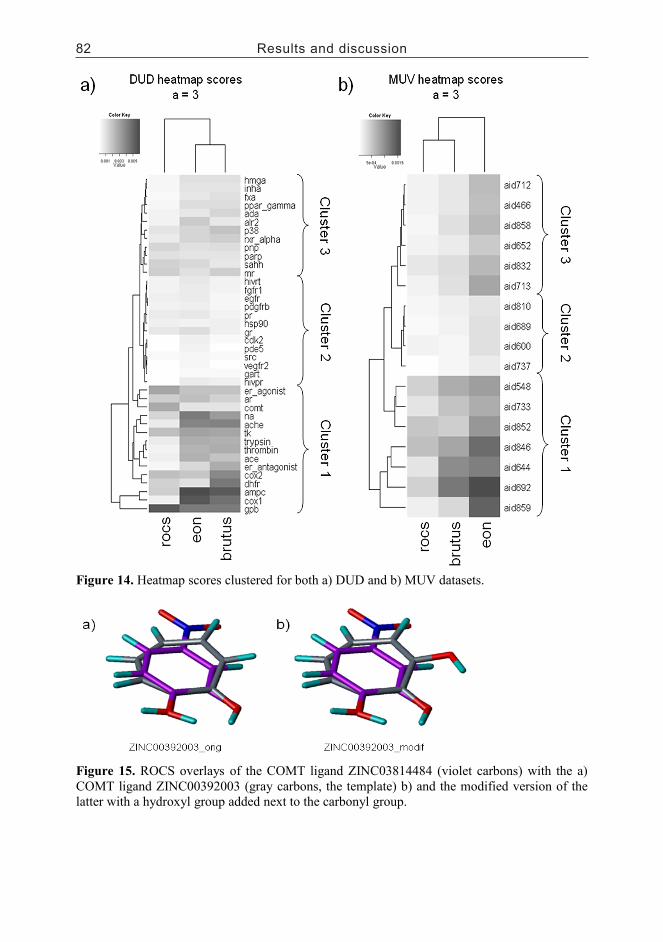
82 Results and discussion
Figure 14. Heatmap scores clustered for both a) DUD and b) MUV datasets.
Figure 15. ROCS overlays of the COMT ligand ZINC03814484 (violet carbons) with the a) COMT ligand ZINC00392003 (gray carbons, the template) b) and the modified version of the latter with a hydroxyl group added next to the carbonyl group.
6 Conclusions
As a result of the thesis work, a new way for fusing virtual screening results has been designed. Not only performing at least as well as existing data fusion techniques the method presented here has the added advantage of interpretability – something that is lost when dealing with just ranks in a list.
Interesting insights on how data fusion works for ligand-based virtual screening tools is presented. The tools whose results are combined should quantify the chemical similarity from different view points. If one tool fails in identifying a pair of chemically similar compounds there is a good chance an orthogonal tool succeeds in this and therefore complementing the first tool. One should also use only three or four tools as it is likely that additional tools are nothing much more than a strain on computational resources and the software license budget.
The performance of the five screening tools evaluated in Publication II was a disappointment. The low enrichment however, is partially an artefact of the benchmark dataset used meaning that there is still room for new and improved benchmark sets. Especially false negatives and alternative binding sites are issues to be taken into account. I hope that the results and discussion that have been presented in this work can serve as a stimulus for people working on the next-generation of benchmark data sets. The third reason for the poor performance – activity cliffs – is a more difficult problem to tackle. Similarity searching methods using only the structural information of actives might not be enough and thus also the information from structurally similar inactives should be included. This is a development that speaks for the use of pharmacophore models where e.g. excluded volumes are routinely used to represent points in space which should be avoided by the ligand.
Quantitative data is crucial in any field for successful decision making. At the same time the use of appropriate visualization techniques should not be underestimated as they make complex data easier for people to comprehend and aid in making conclusions. As part of the thesis work a heatmap plotting technique has been developed to allow the visualization of scaffold hopping patterns of ligand-based virtual screening tools. These are helpful by allowing the user quickly to understand which chemotypes are linked. Also a formula is
presented for turning each heatmap into a number. This not only allows for ranking screening tools based on their scaffold-hopping capability but also allows us to see patterns of the performance for combinations of ligand sets and tools.

Conclusions 83
Figure 14. Heatmap scores clustered for both a) DUD and b) MUV datasets.
Figure 15. ROCS overlays of the COMT ligand ZINC03814484 (violet carbons) with the a) COMT ligand ZINC00392003 (gray carbons, the template) b) and the modified version of the latter with a hydroxyl group added next to the carbonyl group.
6 Conclusions
As a result of the thesis work, a new way for fusing virtual screening results has been designed. Not only performing at least as well as existing data fusion techniques the method presented here has the added advantage of interpretability – something that is lost when dealing with just ranks in a list.
Interesting insights on how data fusion works for ligand-based virtual screening tools is presented. The tools whose results are combined should quantify the chemical similarity from different view points. If one tool fails in identifying a pair of chemically similar compounds there is a good chance an orthogonal tool succeeds in this and therefore complementing the first tool. One should also use only three or four tools as it is likely that additional tools are nothing much more than a strain on computational resources and the software license budget.
The performance of the five screening tools evaluated in Publication II was a disappointment. The low enrichment however, is partially an artefact of the benchmark dataset used meaning that there is still room for new and improved benchmark sets. Especially false negatives and alternative binding sites are issues to be taken into account. I hope that the results and discussion that have been presented in this work can serve as a stimulus for people working on the next-generation of benchmark data sets. The third reason for the poor performance – activity cliffs – is a more difficult problem to tackle. Similarity searching methods using only the structural information of actives might not be enough and thus also the information from structurally similar inactives should be included. This is a development that speaks for the use of pharmacophore models where e.g. excluded volumes are routinely used to represent points in space which should be avoided by the ligand.
Quantitative data is crucial in any field for successful decision making. At the same time the use of appropriate visualization techniques should not be underestimated as they make complex data easier for people to comprehend and aid in making conclusions. As part of the thesis work a heatmap plotting technique has been developed to allow the visualization of scaffold hopping patterns of ligand-based virtual screening tools. These are helpful by allowing the user quickly to understand which chemotypes are linked. Also a formula is
presented for turning each heatmap into a number. This not only allows for ranking screening tools based on their scaffold-hopping capability but also allows us to see patterns of the performance for combinations of ligand sets and tools.

84 Acknowledgements
7 Acknowledgements
The thesis work was carried out at the joint unit of VTT Medical Biotechnology and University of Turku during the years 2005-2009. Working at a unit with connections to both academic and industrial world has been an interesting experience.
I would like to thank my thesis supervisors Professor Olli Kallioniemi (University of Turku) and Professor Antti Poso (University of Kuopio) for their advice and support throughout the five years. I am also grateful to Dr. Lauri Kangas for being member of my thesis committee and the advice he has given. Reviewers of this thesis, Dr. Anna-Marja Hoffrén and Professor Anders Karlén are credited for their work as well.
Over the years I have participated in a number of research projects at our unit. The central driving force behind these has been group leader Dr. Marko Kallio. Other people who have contributed to these projects are Dr. Leena Laine, Jonathan Rehnberg and Mari Björkman.
Many of my colleagues at VTT have become close friends during the past years. I have been lucky for having worked at a work place without major clashes and where people spend time together also outside office hours. I would also like to thank my friends and fellow-modellers at University of Kuopio who I have been able to meet all too rarely. Especially I would like to thank Licenciate of Pharmacy Tuomo Kalliokoski for company during extra-curricular activities of courses and conferences.
During the past two years I have made several visits to University of Innsbruck where I have always felt welcome. I would like to thank Dr. Gerhard Wolber and Professor Thierry Langer for hosting me at their research group. My thanks also go to the co-authors of Publication II: Dr. Patrick Markt, Dr. Johannes Kirchmair and Dr. Simona Distinto.
My research has been funded by Academy of Finland, Sigrid Juselius Foundation, Cancer Organizations of Finland, the Marie Curie Canceromics grant from the EU and the Epitron Project. My many thanks go to these organizations and Professor Olli Kallioniemi for arranging the funding. I have also been member of the ISB graduate school whose annual winter schools in Lapland have been a welcome break in the thesis work and a great opportunity to meet fellow graduate students across the country.
The research projects would not have been possible without the vast computing resources of CSC – IT Center for Science. I would also like to thank Openeye
Scientific Software Inc. and Scitegic Inc. for the free academic licences of the software tools. Dr. Toni Rönkkö is credited for developing the Brutus software used in all Publications of this thesis.
I also want to thank all my friends and family. Many thanks go to my mother Maija and my father Seppo for their support and teaching what is important in life. Finally I want to thank my loving girlfriend Astrid Ziegler for staying by my side despite the great geographical distance that usually has separated us.

Acknowledgements 85
7 Acknowledgements
The thesis work was carried out at the joint unit of VTT Medical Biotechnology and University of Turku during the years 2005-2009. Working at a unit with connections to both academic and industrial world has been an interesting experience.
I would like to thank my thesis supervisors Professor Olli Kallioniemi (University of Turku) and Professor Antti Poso (University of Kuopio) for their advice and support throughout the five years. I am also grateful to Dr. Lauri Kangas for being member of my thesis committee and the advice he has given. Reviewers of this thesis, Dr. Anna-Marja Hoffrén and Professor Anders Karlén are credited for their work as well.
Over the years I have participated in a number of research projects at our unit. The central driving force behind these has been group leader Dr. Marko Kallio. Other people who have contributed to these projects are Dr. Leena Laine, Jonathan Rehnberg and Mari Björkman.
Many of my colleagues at VTT have become close friends during the past years. I have been lucky for having worked at a work place without major clashes and where people spend time together also outside office hours. I would also like to thank my friends and fellow-modellers at University of Kuopio who I have been able to meet all too rarely. Especially I would like to thank Licenciate of Pharmacy Tuomo Kalliokoski for company during extra-curricular activities of courses and conferences.
During the past two years I have made several visits to University of Innsbruck where I have always felt welcome. I would like to thank Dr. Gerhard Wolber and Professor Thierry Langer for hosting me at their research group. My thanks also go to the co-authors of Publication II: Dr. Patrick Markt, Dr. Johannes Kirchmair and Dr. Simona Distinto.
My research has been funded by Academy of Finland, Sigrid Juselius Foundation, Cancer Organizations of Finland, the Marie Curie Canceromics grant from the EU and the Epitron Project. My many thanks go to these organizations and Professor Olli Kallioniemi for arranging the funding. I have also been member of the ISB graduate school whose annual winter schools in Lapland have been a welcome break in the thesis work and a great opportunity to meet fellow graduate students across the country.
The research projects would not have been possible without the vast computing resources of CSC – IT Center for Science. I would also like to thank Openeye
Scientific Software Inc. and Scitegic Inc. for the free academic licences of the software tools. Dr. Toni Rönkkö is credited for developing the Brutus software used in all Publications of this thesis.
I also want to thank all my friends and family. Many thanks go to my mother Maija and my father Seppo for their support and teaching what is important in life. Finally I want to thank my loving girlfriend Astrid Ziegler for staying by my side despite the great geographical distance that usually has separated us.

86 References
8 References
[1] CLARK, M., et al., 1989. Validation of the General Purpose Tripos 5.2 Force Field.Journal of Computational Chemistry,
10(8), pp. 982-1012.
[2] SYBYL atom types.http://tripos.com/mol2/atom_types.html.[3] Rules for Determining Atom Types.http://www.hhmi.swmed.edu/Manuals/csds/pluto/atom_types.html#C.
[4] MENG, E.C. and LEWIS, R.A., 1991.Determination of molecular topology and atomic hybridization states from heavy atom coordinates. Journal of
Computational Chemistry, 12(7), pp. 891-898.
[5] PETTERSEN, E.F., et al., 2004. UCSF Chimera--a visualization system for exploratory research and analysis. Journal of computational chemistry,
25(13), pp. 1605- 1612.
[6] MORRIS, G.M., et al., 1999. Automated docking using a Lamarckian genetic algorithm and an empirical binding free energy function. Journal
of Computational Chemistry, 19(14), pp. 1639-1662.
[7] HILL, R.J., et al., 1988. Determinants of stereospecific binding of type I antiarrhythmic drugs to cardiac sodium channels.Molecular
pharmacology, 34(5), pp. 659-663.
[8] LIM, S.A., 2006. Ethambutol-associated optic neuropathy. Annals of
the Academy of Medicine, Singapore,
35(4), pp. 274-278.
[9] TEO, S.K., et al., 2004. Clinicalpharmacokinetics of thalidomide. Clinical pharmacokinetics, 43(5), pp. 311-327.
[10] LEE, A.C. and CRIPPEN, G.M., 2009. Predicting pKa. Journal of
chemical information and modeling,
49(9), pp. 2013-2033.
[11] KLOPMAN, G. and FERCU, D., 1994. Application Of The Multiple Computer Automated Structure Evaluation Methodology To A Quantitative Structure-Activity Relationship Study Of Acidity. Journal
of Computational Chemistry, 15(9), pp. 1041-1050.
[12] XING, L. and GLEN, R.C., 2002. Novel methods for the prediction of logP, pK(a), and logD. Journal of
chemical information and computer
sciences, 42(4), pp. 796-805.
[13] JELFS, S., et al., 2007. Estimation of pKa for druglike compounds usingsemiempirical and information-baseddescriptors. Journal of chemical
information and modeling, 47(2), pp. 450-459.
[14] KOGEJ, T. and MURESAN, S., 2005. Database mining for pKa prediction. Current drug discovery
technologies, 2(4), pp. 221-229.
[15] MILLETTI, F., et al., 2007. New and original pKa prediction method using grid molecular interaction fields. Journal of chemical information and
modeling, 47(6), pp. 2172-2181.
[16] LIPTAK, M.D., et al., 2002. Absolute pK(a) determinations for substituted phenols.Journal of the
American Chemical Society, 124(22), pp. 6421-6427.
[17] LIPINSKI, C.A., et al., 1997.Experimental and computational approaches to estimate solubility and permeability in drug discovery and development settings. Advanced drug
delivery reviews, 23(1-3), pp. 3-25.
[18] KUBINYI, H., 1979. Nonlineardependence of biological activity onhydrophobic character: the bilinear model. Il Farmaco; edizione
scientifica, 34(3), pp. 248-276.
[19] EISENBERG, D. and MCLACHLAN,A.D., 1986. Solvation energy in protein folding and binding. Nature, 319(6050), pp. 199-203.
[20] MIYAMOTO, S. and KOLLMAN, P.A.,1993. What determines the strength of noncovalent association of ligands to proteins in aqueous solution? Proceedings of the National Academy
of Sciences of the United States of
America, 90(18), pp. 8402-8406.
[21] LEO, A., et al., 1971. Partitioncoefficients and their uses. Chemical
Reviews, 71(6), pp. 525-616.
[22] MORIGUSHI, I., et al., 1992. Simple method of calculating octanol/water partition coefficient. Chemical & Pharmaceutical Bulletin,
40(1), pp. 127-130.
[23] LEO, A.J., 1993. Calculating log Poct from structures. Chemical
Reviews, 93(4), pp.1281-1306.
[24] MOLNAR, L., et al., 2004. A neural network based prediction of octanol-water partition coefficientsusing atomic fragmental descriptors. Bioorganic & medicinal chemistry
letters, 14(4), pp. 851-853.[25] LIAO, Q., et al., 2006. SVM approach for predicting LogP. Molecular diversity, 10(3), pp. 301-309.
[26] GASTEIGER, J. and MARSILI, M., 1980. Iterative partial equalization of orbital electronegativity--a rapid access to atomic charges. Tetrahedron,
36(22), pp. 3219-3228.
[27] GASTEIGER, J. and SALLER, H., 1985. Calculation of the Charge Distribution in Conjugated Systems by a Quantification of the Resonance Concept. Angewandte Chemie
International Edition in English, 24(8), pp.687-689.
[28] SINGER, J.A. and PURCELL, W.P.,1967. Huckel molecular orbital calculations for some antimalarial drugs and related molecules. Journal of
medicinal chemistry, 10(5), pp. 754-762.
References 87
8 References
[1] CLARK, M., et al., 1989. Validation of the General Purpose Tripos 5.2 Force Field.Journal of Computational Chemistry,
10(8), pp. 982-1012.
[2] SYBYL atom types.http://tripos.com/mol2/atom_types.html.[3] Rules for Determining Atom Types.http://www.hhmi.swmed.edu/Manuals/csds/pluto/atom_types.html#C.
[4] MENG, E.C. and LEWIS, R.A., 1991.Determination of molecular topology and atomic hybridization states from heavy atom coordinates. Journal of
Computational Chemistry, 12(7), pp. 891-898.
[5] PETTERSEN, E.F., et al., 2004. UCSF Chimera--a visualization system for exploratory research and analysis. Journal of computational chemistry,
25(13), pp. 1605- 1612.
[6] MORRIS, G.M., et al., 1999. Automated docking using a Lamarckian genetic algorithm and an empirical binding free energy function. Journal
of Computational Chemistry, 19(14), pp. 1639-1662.
[7] HILL, R.J., et al., 1988. Determinants of stereospecific binding of type I antiarrhythmic drugs to cardiac sodium channels.Molecular
pharmacology, 34(5), pp. 659-663.
[8] LIM, S.A., 2006. Ethambutol-associated optic neuropathy. Annals of
the Academy of Medicine, Singapore,
35(4), pp. 274-278.
[9] TEO, S.K., et al., 2004. Clinicalpharmacokinetics of thalidomide. Clinical pharmacokinetics, 43(5), pp. 311-327.
[10] LEE, A.C. and CRIPPEN, G.M., 2009. Predicting pKa. Journal of
chemical information and modeling,
49(9), pp. 2013-2033.
[11] KLOPMAN, G. and FERCU, D., 1994. Application Of The Multiple Computer Automated Structure Evaluation Methodology To A Quantitative Structure-Activity Relationship Study Of Acidity. Journal
of Computational Chemistry, 15(9), pp. 1041-1050.
[12] XING, L. and GLEN, R.C., 2002. Novel methods for the prediction of logP, pK(a), and logD. Journal of
chemical information and computer
sciences, 42(4), pp. 796-805.
[13] JELFS, S., et al., 2007. Estimation of pKa for druglike compounds usingsemiempirical and information-baseddescriptors. Journal of chemical
information and modeling, 47(2), pp. 450-459.
[14] KOGEJ, T. and MURESAN, S., 2005. Database mining for pKa prediction. Current drug discovery
technologies, 2(4), pp. 221-229.
[15] MILLETTI, F., et al., 2007. New and original pKa prediction method using grid molecular interaction fields. Journal of chemical information and
modeling, 47(6), pp. 2172-2181.
[16] LIPTAK, M.D., et al., 2002. Absolute pK(a) determinations for substituted phenols.Journal of the
American Chemical Society, 124(22), pp. 6421-6427.
[17] LIPINSKI, C.A., et al., 1997.Experimental and computational approaches to estimate solubility and permeability in drug discovery and development settings. Advanced drug
delivery reviews, 23(1-3), pp. 3-25.
[18] KUBINYI, H., 1979. Nonlineardependence of biological activity onhydrophobic character: the bilinear model. Il Farmaco; edizione
scientifica, 34(3), pp. 248-276.
[19] EISENBERG, D. and MCLACHLAN,A.D., 1986. Solvation energy in protein folding and binding. Nature, 319(6050), pp. 199-203.
[20] MIYAMOTO, S. and KOLLMAN, P.A.,1993. What determines the strength of noncovalent association of ligands to proteins in aqueous solution? Proceedings of the National Academy
of Sciences of the United States of
America, 90(18), pp. 8402-8406.
[21] LEO, A., et al., 1971. Partitioncoefficients and their uses. Chemical
Reviews, 71(6), pp. 525-616.
[22] MORIGUSHI, I., et al., 1992. Simple method of calculating octanol/water partition coefficient. Chemical & Pharmaceutical Bulletin,
40(1), pp. 127-130.
[23] LEO, A.J., 1993. Calculating log Poct from structures. Chemical
Reviews, 93(4), pp.1281-1306.
[24] MOLNAR, L., et al., 2004. A neural network based prediction of octanol-water partition coefficientsusing atomic fragmental descriptors. Bioorganic & medicinal chemistry
letters, 14(4), pp. 851-853.[25] LIAO, Q., et al., 2006. SVM approach for predicting LogP. Molecular diversity, 10(3), pp. 301-309.
[26] GASTEIGER, J. and MARSILI, M., 1980. Iterative partial equalization of orbital electronegativity--a rapid access to atomic charges. Tetrahedron,
36(22), pp. 3219-3228.
[27] GASTEIGER, J. and SALLER, H., 1985. Calculation of the Charge Distribution in Conjugated Systems by a Quantification of the Resonance Concept. Angewandte Chemie
International Edition in English, 24(8), pp.687-689.
[28] SINGER, J.A. and PURCELL, W.P.,1967. Huckel molecular orbital calculations for some antimalarial drugs and related molecules. Journal of
medicinal chemistry, 10(5), pp. 754-762.

88 References
[29] SCHLICK, T., 1992. OptimizationMethods in Computational Chemistry.Reviews in Computational Chemistry.Editors: Lipkowitz, K.B. and Boyd, D.B. John Wiley & Sons, Inc. New York.
[30] GASTEIGER, J. and ENGEL, T.,(editors), 2003. Chemoinformatics. WILEYVCH Verlag GmbH & Co. Weinheim.
[31] LEACH, A.R., et al., 1990. Automated conformational analysis and structure generation: algorithms for molecular perception. Journal of
Chemical Information and Computer
Sciences, 30(3), pp. 316-324.
[32] LEACH, A.R. and PROUT, K., 1990. Automated conformational analysis: Directed conformational search using the A* algorithm. Journal
of Computational Chemistry, 11(10), pp. 1193-1205.
[33] CORINA. Molecular Networks GmbH. Erlangen, Germany.
[34] CONCORD. Tripos Inc. St. Louis, MO,USA.
[35] KIRCHMAIR, J., et al., 2005.Comparative analysis of protein-bound ligand conformations with respect to catalyst's conformational space subsampling algorithms. Journal of
chemical information and modeling,
45(2), pp. 422-430.
[36] HARDY, L.W. and MALIKAYIL, A.,2003. The impact of structure-guided drug design on clinical agents.
Current Drug Discovery, (Dec), pp. 15-20.
[37] JONES, G., et al., 2009. Elucidating molecular overlays from pairwise alignments using a genetic algorithm. Journal of chemical
information and modeling, 49(7), pp. 1847-1855.
[38] GUNTHER, S., et al., 2006.Representation of target-bound drugs by computed conformers: implications for conformational libraries. BMC
bioinformatics, 7pp. 293.
[39] DAMMKOEHLER, R.A., et al., 1989. Constrained search of conformational hyperspace. Journal of
computer-aided molecular design, 3(1), pp. 3-21.
[40] NICKLAUS, M.C., et al., 1995.Conformational changes of small molecules binding to proteins. Bioorganic & medicinal chemistry,
3(4), pp. 411-428.
[41] BOSTROM, J., et al., 1998.Conformational energy penalties of proteinbound ligands. Journal of
computer-aided molecular design,
12(4), pp. 383-396.
[42] VIETH, M., et al., 1998. Do active site conformations of small ligands correspond to low free-energy solution structures? Journal of computer-aided
molecular design, 12(6),pp. 563-572.
[43] VESTERMANA, B., et al., 1996.Conformer clustering algorithm and itsapplication for crown-type macrocycles. Journal of Molecular
Structure, 368pp. 145-151.
[44] KOHONEN, T., 1982. Self-organized formation of topologically correct feature maps. Biological
Cybernetics, 43(1), pp. 59-69.
[45] OMEGA2. Openeye Scientific Software Inc. Santa Fe, NM, USA.
[46] CHANDRASEKHAR, J., et al., 2001. Efficient exploration of conformational space using the stochastic search method: application to beta-peptide oligomers. Journal of
Computational Chemistry, 22(14), pp.1646-1654.
[47] Catalyst. Accelrys Inc. San Diego, CA, US.
[48] NEWTON, I., 1687. PhilosophiæNaturalis Principia Mathematica.
[49] KIRKPATRICK, S., et al., 1983.Optimization by Simulated Annealing.Science (New York, N.Y.), 220(4598), pp. 671-680.
[50] VAINIO, M.J. and JOHNSON, M.S., 2007. Generating conformer ensembles using a multiobjective genetic algorithm. Journal of
chemical information and modeling,
47(6), pp. 2462-2474.
[51] MAYER, D., et al., 1987. A unique geometry of the active site of angiotensinconverting enzyme consistent with structureactivity
studies. Journal of computer-aided
molecular design, 1(1), pp. 3-16.
[52] HÖLTJE, H.D., et al., 2003. Molecular Modeling: Basic Principles and Application. WILEY-VCH Verlag GmbH & Co. Weinheim.
[53] ALLINGER, N.L., et al., 1989.Molecular mechanics. The MM3 force field for hydrocarbons. 1. Journal of
the American Chemical Society,
111(23), pp. 8551-8566.
[54] ALLINGER, N.L., 1977. Conformational analysis. 130. MM2. A hydrocarbon force field utilizing V1 and V2 torsional terms. Journal of the
American Chemical Society, 99(25), pp. 8127-8134.
[55] HALGREN, T.A., 1999. MMFF VII. Characterization of MMFF94, MMFF94s, and other widely available force fields for conformational energies and for intermolecular-interaction energies and geometries. Journal of
Computational Chemistry, 20(7), pp. 730-748.
[56] BROOKS, B.R., et al., 1983.CHARMM: A Program for Macromolecular Energy, Minimization, and Dynamics Calculations. Journal of
Computational Chemistry, 4(2), pp. 187-217.
[57] CORNELL, W.D., et al., 1995. ASecond Generation Force Field for theSimulation of Proteins, Nucleic Acids, and Organic Molecules. Journal of the
American Chemical Society, 117(19), pp. 5179-5197.

References 89
[29] SCHLICK, T., 1992. OptimizationMethods in Computational Chemistry.Reviews in Computational Chemistry.Editors: Lipkowitz, K.B. and Boyd, D.B. John Wiley & Sons, Inc. New York.
[30] GASTEIGER, J. and ENGEL, T.,(editors), 2003. Chemoinformatics. WILEYVCH Verlag GmbH & Co. Weinheim.
[31] LEACH, A.R., et al., 1990. Automated conformational analysis and structure generation: algorithms for molecular perception. Journal of
Chemical Information and Computer
Sciences, 30(3), pp. 316-324.
[32] LEACH, A.R. and PROUT, K., 1990. Automated conformational analysis: Directed conformational search using the A* algorithm. Journal
of Computational Chemistry, 11(10), pp. 1193-1205.
[33] CORINA. Molecular Networks GmbH. Erlangen, Germany.
[34] CONCORD. Tripos Inc. St. Louis, MO,USA.
[35] KIRCHMAIR, J., et al., 2005.Comparative analysis of protein-bound ligand conformations with respect to catalyst's conformational space subsampling algorithms. Journal of
chemical information and modeling,
45(2), pp. 422-430.
[36] HARDY, L.W. and MALIKAYIL, A.,2003. The impact of structure-guided drug design on clinical agents.
Current Drug Discovery, (Dec), pp. 15-20.
[37] JONES, G., et al., 2009. Elucidating molecular overlays from pairwise alignments using a genetic algorithm. Journal of chemical
information and modeling, 49(7), pp. 1847-1855.
[38] GUNTHER, S., et al., 2006.Representation of target-bound drugs by computed conformers: implications for conformational libraries. BMC
bioinformatics, 7pp. 293.
[39] DAMMKOEHLER, R.A., et al., 1989. Constrained search of conformational hyperspace. Journal of
computer-aided molecular design, 3(1), pp. 3-21.
[40] NICKLAUS, M.C., et al., 1995.Conformational changes of small molecules binding to proteins. Bioorganic & medicinal chemistry,
3(4), pp. 411-428.
[41] BOSTROM, J., et al., 1998.Conformational energy penalties of proteinbound ligands. Journal of
computer-aided molecular design,
12(4), pp. 383-396.
[42] VIETH, M., et al., 1998. Do active site conformations of small ligands correspond to low free-energy solution structures? Journal of computer-aided
molecular design, 12(6),pp. 563-572.
[43] VESTERMANA, B., et al., 1996.Conformer clustering algorithm and itsapplication for crown-type macrocycles. Journal of Molecular
Structure, 368pp. 145-151.
[44] KOHONEN, T., 1982. Self-organized formation of topologically correct feature maps. Biological
Cybernetics, 43(1), pp. 59-69.
[45] OMEGA2. Openeye Scientific Software Inc. Santa Fe, NM, USA.
[46] CHANDRASEKHAR, J., et al., 2001. Efficient exploration of conformational space using the stochastic search method: application to beta-peptide oligomers. Journal of
Computational Chemistry, 22(14), pp.1646-1654.
[47] Catalyst. Accelrys Inc. San Diego, CA, US.
[48] NEWTON, I., 1687. PhilosophiæNaturalis Principia Mathematica.
[49] KIRKPATRICK, S., et al., 1983.Optimization by Simulated Annealing.Science (New York, N.Y.), 220(4598), pp. 671-680.
[50] VAINIO, M.J. and JOHNSON, M.S., 2007. Generating conformer ensembles using a multiobjective genetic algorithm. Journal of
chemical information and modeling,
47(6), pp. 2462-2474.
[51] MAYER, D., et al., 1987. A unique geometry of the active site of angiotensinconverting enzyme consistent with structureactivity
studies. Journal of computer-aided
molecular design, 1(1), pp. 3-16.
[52] HÖLTJE, H.D., et al., 2003. Molecular Modeling: Basic Principles and Application. WILEY-VCH Verlag GmbH & Co. Weinheim.
[53] ALLINGER, N.L., et al., 1989.Molecular mechanics. The MM3 force field for hydrocarbons. 1. Journal of
the American Chemical Society,
111(23), pp. 8551-8566.
[54] ALLINGER, N.L., 1977. Conformational analysis. 130. MM2. A hydrocarbon force field utilizing V1 and V2 torsional terms. Journal of the
American Chemical Society, 99(25), pp. 8127-8134.
[55] HALGREN, T.A., 1999. MMFF VII. Characterization of MMFF94, MMFF94s, and other widely available force fields for conformational energies and for intermolecular-interaction energies and geometries. Journal of
Computational Chemistry, 20(7), pp. 730-748.
[56] BROOKS, B.R., et al., 1983.CHARMM: A Program for Macromolecular Energy, Minimization, and Dynamics Calculations. Journal of
Computational Chemistry, 4(2), pp. 187-217.
[57] CORNELL, W.D., et al., 1995. ASecond Generation Force Field for theSimulation of Proteins, Nucleic Acids, and Organic Molecules. Journal of the
American Chemical Society, 117(19), pp. 5179-5197.

90 References
[58] JORGENSEN, W.L. and TIRADORIVES, J., 1988. The OPLS [optimized potentials for liquid simulations] potential functions for proteins, energy minimizations for crystals of cyclic peptides and crambin.Journal of the American Chemical
Society, 110(6), pp. 1657-1666.
[59] CHRISTEN, M., et al., 2005. TheGROMOS software for biomolecularsimulation: GROMOS05. Journal of
computational chemistry, 26(16), pp. 1719-1751.
[60] KELLOGG, G.E., et al., 1991. HINT: a new method of empirical hydrophobic field calculation for CoMFA. Journal of computer aided
molecular design, 5(6), pp. 545-552.
[61] VERDONK, M.L., et al., 1999.SuperStar: a knowledge-based approach for identifying interaction sites in proteins.Journal of Molecular
Biology, 289(4), pp.1093-1108.
[62] GOODFORD, P.J., 1985. Acomputational procedure fordetermining energetically favorable binding sites on biologically important macromolecules. Journal of medicinal
chemistry, 28(7), pp.849-857.
[63] CRUCIANI, G., (editor), 2006.Molecular Interaction Fields. WILEY-VCH Verlag GmbH & Co. Weinheim.
[64] GRID manual: Computing thehydrophobic energies.http://www.moldiscovery.com/docs/grid/c43.html.
[65] GRID manual: Directives controlling the choice of the probe.http://www.moldiscovery.com/docs/grid/c4458.html.
[66] VON ITZSTEIN, M., et al., 1993.Rational design of potent sialidase-based inhibitors of influenza virus replication. Nature, 363(6428), pp. 418-423.
[67] BARONI, M., et al., 2007. A common reference framework for analyzing/comparing proteins and ligands. Fingerprints for Ligandsand Proteins (FLAP): theory and application. Journal of chemical
information and modeling, 47(2), pp. 279-294.
[68] MARTIN, Y.C., et al., 2002. Dostructurally similar molecules have similar biological activity? Journal of
medicinal chemistry, 45(19), pp. 4350-4358.
[69] DURANT, J.L., et al., 2002.Reoptimization of MDL keys for use in drug discovery. Journal of chemical
information and computer sciences,
42(6), pp. 1273-1280.
[70] Fingerprints - Screening and Similarity. http://www.daylight.com/dayhtml/doc/theory/theory.finger.html.
[71] SCITEGIC, Inc., 2007. Pipeline Pilot. Chemistry Collection: Basic Chemistry Guide. Scitegic, Inc. San Diego, CA, US.
[72] Pipeline Pilot Student Edition. Accelrys Inc.
[73] FLOWER, D.R., 1998. On the Properties of Bit String-Based Measures of Chemical Similarity. Journal of Chemical Information
and Computer Sciences, 38(3), pp. 379-386.
[74] HOLLIDAY, J.D., et al., 2003. Analysis and display of the size dependence of chemical similarity coefficients. Journal of chemical
information and computer sciences,
43(3), pp. 819-828.
[75] FLIGNER, M.A., et al., 2002. AModification of the Jaccard-TanimotoSimilarity Index for Diverse Selection of Chemical Compounds Using Binary Strings. Technometrics, 44pp. 110-119.
[76] CLEVES, A.E. and JAIN, A.N., 2008. Effects of inductive bias on computational evaluations of ligand-based modeling and on drug discovery. Journal of computer-aided molecular
design, 22(3-4), pp. 147-159.
[77] WRIGHT, P.J., 2006. Comparison of phosphodiesterase type 5 (PDE5) inhibitors.International journal of
clinical practice, 60(8), pp. 967-975.
[78] SUPURAN, C.T., et al., 2006.Phosphodiesterase 5 inhibitors--drug design and differentiation based on selectivity, pharmacokinetic and efficacy profiles. Current
pharmaceutical design, 12(27), pp.3459-3465.
[79] MCGAUGHEY, G.B., et al., 2007.Comparison of topological, shape, anddocking methods in virtual screening. Journal of chemical information and
modeling, 47(4), pp. 1504-1519.
[80] HAWKINS, P.C., et al., 2007.Comparison of shape-matching and docking as virtual screening tools. Journal of medicinal chemistry, 50(1), pp. 74-82.
[81] RONKKO, T., et al., 2006. BRUTUS: optimization of a grid-based similarity function for rigid-body molecular superposition. II. Description and characterization. Journal of
computer-aided molecular design,
20(4), pp. 227-236.
[82] TERVO, A.J., et al., 2005. BRUTUS: optimization of a grid-based similarity function for rigid-body molecular superposition. 1. Alignment and virtual screening applications. Journal of medicinal chemistry, 48(12), pp. 4076-4086.
[83] RÖNKKÖ, T.P., 2009. A Molecular Energy Field Based Superposition Algorithm for Virtual Screening. Dissertation/Thesis. University of Kuopio.
[84] CHEESERIGHT, T.J., et al., 2008.FieldScreen: virtual screening usingmolecular fields. Application to the DUD data set. Journal of chemical
information and modeling, 48(11), pp. 2108-2117.
References 91
[58] JORGENSEN, W.L. and TIRADORIVES, J., 1988. The OPLS [optimized potentials for liquid simulations] potential functions for proteins, energy minimizations for crystals of cyclic peptides and crambin.Journal of the American Chemical
Society, 110(6), pp. 1657-1666.
[59] CHRISTEN, M., et al., 2005. TheGROMOS software for biomolecularsimulation: GROMOS05. Journal of
computational chemistry, 26(16), pp. 1719-1751.
[60] KELLOGG, G.E., et al., 1991. HINT: a new method of empirical hydrophobic field calculation for CoMFA. Journal of computer aided
molecular design, 5(6), pp. 545-552.
[61] VERDONK, M.L., et al., 1999.SuperStar: a knowledge-based approach for identifying interaction sites in proteins.Journal of Molecular
Biology, 289(4), pp.1093-1108.
[62] GOODFORD, P.J., 1985. Acomputational procedure fordetermining energetically favorable binding sites on biologically important macromolecules. Journal of medicinal
chemistry, 28(7), pp.849-857.
[63] CRUCIANI, G., (editor), 2006.Molecular Interaction Fields. WILEY-VCH Verlag GmbH & Co. Weinheim.
[64] GRID manual: Computing thehydrophobic energies.http://www.moldiscovery.com/docs/grid/c43.html.
[65] GRID manual: Directives controlling the choice of the probe.http://www.moldiscovery.com/docs/grid/c4458.html.
[66] VON ITZSTEIN, M., et al., 1993.Rational design of potent sialidase-based inhibitors of influenza virus replication. Nature, 363(6428), pp. 418-423.
[67] BARONI, M., et al., 2007. A common reference framework for analyzing/comparing proteins and ligands. Fingerprints for Ligandsand Proteins (FLAP): theory and application. Journal of chemical
information and modeling, 47(2), pp. 279-294.
[68] MARTIN, Y.C., et al., 2002. Dostructurally similar molecules have similar biological activity? Journal of
medicinal chemistry, 45(19), pp. 4350-4358.
[69] DURANT, J.L., et al., 2002.Reoptimization of MDL keys for use in drug discovery. Journal of chemical
information and computer sciences,
42(6), pp. 1273-1280.
[70] Fingerprints - Screening and Similarity. http://www.daylight.com/dayhtml/doc/theory/theory.finger.html.
[71] SCITEGIC, Inc., 2007. Pipeline Pilot. Chemistry Collection: Basic Chemistry Guide. Scitegic, Inc. San Diego, CA, US.
[72] Pipeline Pilot Student Edition. Accelrys Inc.
[73] FLOWER, D.R., 1998. On the Properties of Bit String-Based Measures of Chemical Similarity. Journal of Chemical Information
and Computer Sciences, 38(3), pp. 379-386.
[74] HOLLIDAY, J.D., et al., 2003. Analysis and display of the size dependence of chemical similarity coefficients. Journal of chemical
information and computer sciences,
43(3), pp. 819-828.
[75] FLIGNER, M.A., et al., 2002. AModification of the Jaccard-TanimotoSimilarity Index for Diverse Selection of Chemical Compounds Using Binary Strings. Technometrics, 44pp. 110-119.
[76] CLEVES, A.E. and JAIN, A.N., 2008. Effects of inductive bias on computational evaluations of ligand-based modeling and on drug discovery. Journal of computer-aided molecular
design, 22(3-4), pp. 147-159.
[77] WRIGHT, P.J., 2006. Comparison of phosphodiesterase type 5 (PDE5) inhibitors.International journal of
clinical practice, 60(8), pp. 967-975.
[78] SUPURAN, C.T., et al., 2006.Phosphodiesterase 5 inhibitors--drug design and differentiation based on selectivity, pharmacokinetic and efficacy profiles. Current
pharmaceutical design, 12(27), pp.3459-3465.
[79] MCGAUGHEY, G.B., et al., 2007.Comparison of topological, shape, anddocking methods in virtual screening. Journal of chemical information and
modeling, 47(4), pp. 1504-1519.
[80] HAWKINS, P.C., et al., 2007.Comparison of shape-matching and docking as virtual screening tools. Journal of medicinal chemistry, 50(1), pp. 74-82.
[81] RONKKO, T., et al., 2006. BRUTUS: optimization of a grid-based similarity function for rigid-body molecular superposition. II. Description and characterization. Journal of
computer-aided molecular design,
20(4), pp. 227-236.
[82] TERVO, A.J., et al., 2005. BRUTUS: optimization of a grid-based similarity function for rigid-body molecular superposition. 1. Alignment and virtual screening applications. Journal of medicinal chemistry, 48(12), pp. 4076-4086.
[83] RÖNKKÖ, T.P., 2009. A Molecular Energy Field Based Superposition Algorithm for Virtual Screening. Dissertation/Thesis. University of Kuopio.
[84] CHEESERIGHT, T.J., et al., 2008.FieldScreen: virtual screening usingmolecular fields. Application to the DUD data set. Journal of chemical
information and modeling, 48(11), pp. 2108-2117.

92 References
[85] CHEESERIGHT, T., et al., 2006.Molecular field extrema as descriptors of biological activity: definition and validation. Journal of chemical
information and modeling, 46(2), pp. 665-676.
[86] VAINIO, M.J., et al., 2009. ShaEP: molecular overlay based on shape and electrostatic potential. Journal of chemical information and
modeling, 49(2), pp. 492-502.
[87] ROCS. Openeye Scientific Software Inc.
[88] NICHOLLS, A., et al., 2004. Variable selection and model validation of 2D and 3D molecular descriptors. Journal of computeraided molecular
design, 18(7-9), pp. 451-474.
[89] GRANT, J.A., et al., 1998. A fastmethod of molecular shape comparison: A simple application of a Gaussian description of molecular shape. Journal
of Computational Chemistry, 17(14), pp. 1653-1666.
[90] WERMUTH, C., et al., 1998. Glossary of Terms Used in Medicinal Chemistry (IUPAC Recommendations 1997).
[91] LANGER, T. and HOFFMANN, R.D., (editors), 2006. Pharmacophores and Pharmacophore Searches. WILEY-VCH Verlag GmbH & Co. Weinheim.
[92] WOLBER, G. and LANGER, T., 2005. LigandScout: 3-D pharmacophores derived from protein-bound ligands and their use as virtual screening filters. Journal of chemical
information and modeling, 45(1), pp. 160-169.
[93] RICHMOND, N.J., et al., 2006.GALAHAD: 1. pharmacophore identification by hypermolecular alignment of ligands in 3D. Journal of
computer-aided molecular design,
20(9), pp. 567-587.
[94] JONES, G., et al., 1995. A geneticalgorithm for flexible molecular overlay and pharmacophore elucidation. Journal of computer-aided
molecular design, 9(6), pp. 532-549.
[95] TOBA, S., et al., 2006. Usingpharmacophore models to gain insight into structural binding and virtual screening: an application study with CDK2 and human DHFR. Journal of
chemical information and modeling,
46(2), pp. 728-735.
[96] RCSB Protein Data Bank.http://www.rcsb.org/pdb/home/home.do.
[97] DIXON, S.L., et al., 2006. PHASE: a new engine for pharmacophore perception, 3D QSAR model development, and 3D database screening: 1. Methodology and preliminary results. Journal of
computeraided molecular design,
20(10-11), pp. 647-671.
[98] JONES, G., et al., 1997. Development and validation of a genetic algorithm for flexible docking. Journal of Molecular Biology, 267(3), pp. 727-748.
[99] EWING, T.J., et al., 2001. DOCK 4.0: search strategies for automated molecular docking of flexible molecule databases. Journal of computer-aided
molecular design, 15(5), pp. 411-428.
[100] FlexX. http://www.biosolveit.de/FlexX/.
[101] FRED. Openeye Scientific Software Inc. Santa Fe, NM, USA.
[102] MUEGGE, I. and MARTIN, Y.C., 1999. A general and fast scoring function for protein-ligand interactions: a simplified potential approach. Journal of medicinal chemistry, 42(5), pp. 791-804.
[103] STAHL, M. and SCHULZ-GASCH, T., 2004. Scoring functions for protein–ligand interactions: a critical perspective. Drug Discovery
Today: Technologies, 1(3), pp.231-239.
[104] BAXTER, C.A., et al., 1998. Flexible docking using Tabu search and an empirical estimate of binding affinity. Proteins, 33(3), pp. 367-382.
[105] ELDRIDGE, M.D., et al., 1997.Empirical scoring functions: I. Thedevelopment of a fast empirical scoringfunction to estimate the binding affinity of ligands in receptor complexes. Journal of computer-aided molecular
design, 11(5), pp. 425-445.
[106] O'BOYLE, N.M., et al., 2008. Using buriedness to improve discrimination between actives and inactives in docking. Journal of
chemical information and modeling,
48(6), pp. 1269-1278.
[107] DENG, Z., et al., 2004. Structuralinteraction fingerprint (SIFt): a novel method for analyzing three-dimensional proteinligand binding interactions. Journal of medicinal chemistry, 47(2), pp. 337-344.
[108] RADESTOCK, S., et al., 2008.Homology model-based virtual screening for GPCR ligands using docking and target biased scoring. Journal of chemical information and
modeling, 48(5), pp. 1104-1117.
[109] ENYEDY, I.J. and EGAN, W.J., 2008. Can we use docking and scoring for hit-tolead optimization? Journal of
computer-aided molecular design,
22(3-4), pp. 161-168.
[110] PAGE, C.S. and BATES, P.A., 2006. Can MM-PBSA calculations predict the specificities of protein kinase inhibitors? Journal of
computational chemistry, 27(16),pp. 1990-2007.
[111] COUPEZ, B. and LEWIS, R.A., 2006. Docking and scoring--theoretically easy, practically impossible? Current medicinal
chemistry, 13(25), pp. 2995-3003.
[112] NAJMANOVICH, R., et al., 2000. Side-chain flexibility in proteins upon ligand binding. Proteins, 39(3), pp. 261-268.
[113] CARLSON, H.A., 2002. Proteinflexibility and drug design: how to hit amoving target. Current opinion in
chemical biology, 6(4), pp. 447-452.
References 93
[85] CHEESERIGHT, T., et al., 2006.Molecular field extrema as descriptors of biological activity: definition and validation. Journal of chemical
information and modeling, 46(2), pp. 665-676.
[86] VAINIO, M.J., et al., 2009. ShaEP: molecular overlay based on shape and electrostatic potential. Journal of chemical information and
modeling, 49(2), pp. 492-502.
[87] ROCS. Openeye Scientific Software Inc.
[88] NICHOLLS, A., et al., 2004. Variable selection and model validation of 2D and 3D molecular descriptors. Journal of computeraided molecular
design, 18(7-9), pp. 451-474.
[89] GRANT, J.A., et al., 1998. A fastmethod of molecular shape comparison: A simple application of a Gaussian description of molecular shape. Journal
of Computational Chemistry, 17(14), pp. 1653-1666.
[90] WERMUTH, C., et al., 1998. Glossary of Terms Used in Medicinal Chemistry (IUPAC Recommendations 1997).
[91] LANGER, T. and HOFFMANN, R.D., (editors), 2006. Pharmacophores and Pharmacophore Searches. WILEY-VCH Verlag GmbH & Co. Weinheim.
[92] WOLBER, G. and LANGER, T., 2005. LigandScout: 3-D pharmacophores derived from protein-bound ligands and their use as virtual screening filters. Journal of chemical
information and modeling, 45(1), pp. 160-169.
[93] RICHMOND, N.J., et al., 2006.GALAHAD: 1. pharmacophore identification by hypermolecular alignment of ligands in 3D. Journal of
computer-aided molecular design,
20(9), pp. 567-587.
[94] JONES, G., et al., 1995. A geneticalgorithm for flexible molecular overlay and pharmacophore elucidation. Journal of computer-aided
molecular design, 9(6), pp. 532-549.
[95] TOBA, S., et al., 2006. Usingpharmacophore models to gain insight into structural binding and virtual screening: an application study with CDK2 and human DHFR. Journal of
chemical information and modeling,
46(2), pp. 728-735.
[96] RCSB Protein Data Bank.http://www.rcsb.org/pdb/home/home.do.
[97] DIXON, S.L., et al., 2006. PHASE: a new engine for pharmacophore perception, 3D QSAR model development, and 3D database screening: 1. Methodology and preliminary results. Journal of
computeraided molecular design,
20(10-11), pp. 647-671.
[98] JONES, G., et al., 1997. Development and validation of a genetic algorithm for flexible docking. Journal of Molecular Biology, 267(3), pp. 727-748.
[99] EWING, T.J., et al., 2001. DOCK 4.0: search strategies for automated molecular docking of flexible molecule databases. Journal of computer-aided
molecular design, 15(5), pp. 411-428.
[100] FlexX. http://www.biosolveit.de/FlexX/.
[101] FRED. Openeye Scientific Software Inc. Santa Fe, NM, USA.
[102] MUEGGE, I. and MARTIN, Y.C., 1999. A general and fast scoring function for protein-ligand interactions: a simplified potential approach. Journal of medicinal chemistry, 42(5), pp. 791-804.
[103] STAHL, M. and SCHULZ-GASCH, T., 2004. Scoring functions for protein–ligand interactions: a critical perspective. Drug Discovery
Today: Technologies, 1(3), pp.231-239.
[104] BAXTER, C.A., et al., 1998. Flexible docking using Tabu search and an empirical estimate of binding affinity. Proteins, 33(3), pp. 367-382.
[105] ELDRIDGE, M.D., et al., 1997.Empirical scoring functions: I. Thedevelopment of a fast empirical scoringfunction to estimate the binding affinity of ligands in receptor complexes. Journal of computer-aided molecular
design, 11(5), pp. 425-445.
[106] O'BOYLE, N.M., et al., 2008. Using buriedness to improve discrimination between actives and inactives in docking. Journal of
chemical information and modeling,
48(6), pp. 1269-1278.
[107] DENG, Z., et al., 2004. Structuralinteraction fingerprint (SIFt): a novel method for analyzing three-dimensional proteinligand binding interactions. Journal of medicinal chemistry, 47(2), pp. 337-344.
[108] RADESTOCK, S., et al., 2008.Homology model-based virtual screening for GPCR ligands using docking and target biased scoring. Journal of chemical information and
modeling, 48(5), pp. 1104-1117.
[109] ENYEDY, I.J. and EGAN, W.J., 2008. Can we use docking and scoring for hit-tolead optimization? Journal of
computer-aided molecular design,
22(3-4), pp. 161-168.
[110] PAGE, C.S. and BATES, P.A., 2006. Can MM-PBSA calculations predict the specificities of protein kinase inhibitors? Journal of
computational chemistry, 27(16),pp. 1990-2007.
[111] COUPEZ, B. and LEWIS, R.A., 2006. Docking and scoring--theoretically easy, practically impossible? Current medicinal
chemistry, 13(25), pp. 2995-3003.
[112] NAJMANOVICH, R., et al., 2000. Side-chain flexibility in proteins upon ligand binding. Proteins, 39(3), pp. 261-268.
[113] CARLSON, H.A., 2002. Proteinflexibility and drug design: how to hit amoving target. Current opinion in
chemical biology, 6(4), pp. 447-452.

94 References
[114] TEAGUE, S.J., 2003. Implications of protein flexibility for drug discovery. Nature reviews.Drug
discovery, 2(7), pp. 527-541.
[115] TOTROV, M. and ABAGYAN, R.,2008. Flexible ligand docking to multiple receptor conformations: a practical alternative. Current opinion in
structural biology, 18(2), pp. 178-184.
[116] JIANG, F. and KIM, S.H., 1991. "Soft docking": matching of molecular surface cubes. Journal of Molecular
Biology, 219(1),pp. 79-102.
[117] BARRIL, X. and MORLEY, S.D.,2005. Unveiling the full potential of flexible receptor docking using multiple crystallographic structures. Journal of medicinal chemistry, 48(13), pp. 4432-4443.
[118] LEACH, A.R., 1994. Ligand docking to proteins with discrete side-chain flexibility.Journal of Molecular
Biology, 235(1), pp.345-356.
[119] ALONSO, H., et al., 2006. Combining docking and molecular dynamic simulations in drug design. Medicinal research reviews, 26(5), pp. 531-568.
[120] SHERMAN, W., et al., 2006. Novel procedure for modeling ligand/receptor induced fit effects. Journal of medicinal chemistry, 49(2), pp. 534-553.
[121] MDL Drug Data Report.http://www.symyx.com/products/databases/bioactivity/mddr/index.jsp.
[122] MACKEY, M.D. and MELVILLE, J.L.,2009. Better than random? The chemotype enrichment problem. Journal of chemical
information and modeling, 49(5), pp. 1154-1162.
[123] HUANG, N., et al., 2006.Benchmarking sets for molecular docking. Journal of medicinal
chemistry, 49(23), pp.6789-6801.
[124] HAWKINS, P.C., et al., 2008. How to do an evaluation: pitfalls and traps. Journal of computer-aided
molecular design, 22(3-4), pp. 179-190.
[125] BISSANTZ, C., et al., 2000. Protein-based virtual screening of chemical databases. 1. Evaluation of different docking/scoring combinations. Journal of medicinal chemistry, 43(25), pp. 4759-4767.
[126] VERDONK, M.L., et al., 2004. Virtual screening using protein-ligand docking: avoiding artificial enrichment. Journal of chemical information and
computer sciences, 44(3), pp. 793-806.
[127] IRWIN, J.J. and SHOICHET, B.K.,2005. ZINC--a free database of commercially available compounds for virtual screening.Journal of chemical
information and modeling, 45(1), pp. 177-182.
[128] IHLENFELDT, W.D., et al., 1994. Computation and management of chemical properties in CACTVS: An extensible networked approach toward modularity and compatibility. Journal
of Chemical Information and Computer
Sciences, 34(1), pp. 109-116.[129] KIRCHMAIR, J., et al., 2009. How to optimize shape-based virtual screening: choosing the right query and including chemical information. Journal of chemical information and
modeling, 49(3), pp. 678-692.
[130] VON KORFF, M., et al., 2009.Comparison of ligand- and structure-based virtual screening on the DUD data set. Journal of chemical
information and modeling, 49(2), pp. 209-231.
[131] IRWIN, J.J., 2008. Communitybenchmarks for virtual screening. Journal of computer-aided molecular
design, 22(3-4), pp. 193-199.
[132] GOOD, A.C. and OPREA, T.I., 2008. Optimization of CAMD techniques 3. Virtual screening enrichment studies: a help or hindrance in tool selection? Journal ofcomputer-
aided molecular design, 22(3-4),pp. 169-178.
[133] ROHRER, S.G. and BAUMANN, K., 2009. Maximum unbiased validation (MUV)data sets for virtual screening based onPubChem bioactivity data. Journal of
chemical information and modeling,
49(2), pp. 169-184.
[134] WHEELER, D.L., et al., 2008.Database resources of the National Center for Biotechnology Information. Nucleic acids research, 36(Database issue), pp. D13-21.
[135] The Pubchem Project.http://pubchem.ncbi.nlm.nih.gov/.
[136] FAWCETT, T., 2006. An introduction to ROC analysis. Pattern
Recognition Letters, 27(8), pp. 861-874.
[137] JAIN, A.N., 2008. Bias, reporting, and sharing: computational evaluations of docking methods. Journal of computer-aided molecular
design, 22(3-4), pp. 201-212.
[138] TRUCHON, J.F. and BAYLY, C.I.,2007. Evaluating virtual screening methods: good and bad metrics for the "early recognition" problem. Journal of
chemical information and modeling,
47(2), pp. 488-508.
[139] GOOD, A.C., et al., 2004. Measuring CAMD technique performance: a virtual screening case study in the design of validation experiments. Journal of computer
aided molecular design, 18(7-9), pp. 529-536.
[140] CLARK, R.D. and WEBSTERCLARK, D.J., 2008. Managing bias in ROC curves. Journal
of computer-aided molecular design,
22(3-4), pp. 141-146.[141] KIRCHMAIR, J., et al., 2006.Comparative performance assessment of the conformational model generators omega and catalyst: a large-scale survey on the retrieval of protein-bound ligand conformations. Journal of
chemical information and modeling,
46(4), pp. 1848-1861.

References 95
[114] TEAGUE, S.J., 2003. Implications of protein flexibility for drug discovery. Nature reviews.Drug
discovery, 2(7), pp. 527-541.
[115] TOTROV, M. and ABAGYAN, R.,2008. Flexible ligand docking to multiple receptor conformations: a practical alternative. Current opinion in
structural biology, 18(2), pp. 178-184.
[116] JIANG, F. and KIM, S.H., 1991. "Soft docking": matching of molecular surface cubes. Journal of Molecular
Biology, 219(1),pp. 79-102.
[117] BARRIL, X. and MORLEY, S.D.,2005. Unveiling the full potential of flexible receptor docking using multiple crystallographic structures. Journal of medicinal chemistry, 48(13), pp. 4432-4443.
[118] LEACH, A.R., 1994. Ligand docking to proteins with discrete side-chain flexibility.Journal of Molecular
Biology, 235(1), pp.345-356.
[119] ALONSO, H., et al., 2006. Combining docking and molecular dynamic simulations in drug design. Medicinal research reviews, 26(5), pp. 531-568.
[120] SHERMAN, W., et al., 2006. Novel procedure for modeling ligand/receptor induced fit effects. Journal of medicinal chemistry, 49(2), pp. 534-553.
[121] MDL Drug Data Report.http://www.symyx.com/products/databases/bioactivity/mddr/index.jsp.
[122] MACKEY, M.D. and MELVILLE, J.L.,2009. Better than random? The chemotype enrichment problem. Journal of chemical
information and modeling, 49(5), pp. 1154-1162.
[123] HUANG, N., et al., 2006.Benchmarking sets for molecular docking. Journal of medicinal
chemistry, 49(23), pp.6789-6801.
[124] HAWKINS, P.C., et al., 2008. How to do an evaluation: pitfalls and traps. Journal of computer-aided
molecular design, 22(3-4), pp. 179-190.
[125] BISSANTZ, C., et al., 2000. Protein-based virtual screening of chemical databases. 1. Evaluation of different docking/scoring combinations. Journal of medicinal chemistry, 43(25), pp. 4759-4767.
[126] VERDONK, M.L., et al., 2004. Virtual screening using protein-ligand docking: avoiding artificial enrichment. Journal of chemical information and
computer sciences, 44(3), pp. 793-806.
[127] IRWIN, J.J. and SHOICHET, B.K.,2005. ZINC--a free database of commercially available compounds for virtual screening.Journal of chemical
information and modeling, 45(1), pp. 177-182.
[128] IHLENFELDT, W.D., et al., 1994. Computation and management of chemical properties in CACTVS: An extensible networked approach toward modularity and compatibility. Journal
of Chemical Information and Computer
Sciences, 34(1), pp. 109-116.[129] KIRCHMAIR, J., et al., 2009. How to optimize shape-based virtual screening: choosing the right query and including chemical information. Journal of chemical information and
modeling, 49(3), pp. 678-692.
[130] VON KORFF, M., et al., 2009.Comparison of ligand- and structure-based virtual screening on the DUD data set. Journal of chemical
information and modeling, 49(2), pp. 209-231.
[131] IRWIN, J.J., 2008. Communitybenchmarks for virtual screening. Journal of computer-aided molecular
design, 22(3-4), pp. 193-199.
[132] GOOD, A.C. and OPREA, T.I., 2008. Optimization of CAMD techniques 3. Virtual screening enrichment studies: a help or hindrance in tool selection? Journal ofcomputer-
aided molecular design, 22(3-4),pp. 169-178.
[133] ROHRER, S.G. and BAUMANN, K., 2009. Maximum unbiased validation (MUV)data sets for virtual screening based onPubChem bioactivity data. Journal of
chemical information and modeling,
49(2), pp. 169-184.
[134] WHEELER, D.L., et al., 2008.Database resources of the National Center for Biotechnology Information. Nucleic acids research, 36(Database issue), pp. D13-21.
[135] The Pubchem Project.http://pubchem.ncbi.nlm.nih.gov/.
[136] FAWCETT, T., 2006. An introduction to ROC analysis. Pattern
Recognition Letters, 27(8), pp. 861-874.
[137] JAIN, A.N., 2008. Bias, reporting, and sharing: computational evaluations of docking methods. Journal of computer-aided molecular
design, 22(3-4), pp. 201-212.
[138] TRUCHON, J.F. and BAYLY, C.I.,2007. Evaluating virtual screening methods: good and bad metrics for the "early recognition" problem. Journal of
chemical information and modeling,
47(2), pp. 488-508.
[139] GOOD, A.C., et al., 2004. Measuring CAMD technique performance: a virtual screening case study in the design of validation experiments. Journal of computer
aided molecular design, 18(7-9), pp. 529-536.
[140] CLARK, R.D. and WEBSTERCLARK, D.J., 2008. Managing bias in ROC curves. Journal
of computer-aided molecular design,
22(3-4), pp. 141-146.[141] KIRCHMAIR, J., et al., 2006.Comparative performance assessment of the conformational model generators omega and catalyst: a large-scale survey on the retrieval of protein-bound ligand conformations. Journal of
chemical information and modeling,
46(4), pp. 1848-1861.
96 References
[142] SHAFER, G., 1986.The combination of evidence. International Journal of Intelligent
Systems, 1(3), pp. 155-179.
[143] HALL, D.L. and MCMULLEN, S.A.H., 2004. Mathematical Techniques in Multisensor Data Fusion. Artech House, Inc. Norwood, MA.
[144] WILLETT, P., 2006. Enhancing the Effectiveness of Ligand-Based Virtual Screening Using Data Fusion. QSAR & Combinatoral Science, 25(12), pp. 1143-1152.
[145] WHITTLE, M., et al., 2006. Analysis of data fusion methods in virtual screening: similarity and group fusion. Journal of chemical
information and modeling, 46(6),pp. 2206-2219.
[146] WHITTLE, M., et al., 2003. Evaluation of similarity measures for searching the dictionary of natural products database. Journal of chemical
information and computer sciences,
43(2), pp. 449-457.
[147] WANG, R. and WANG, S., 2001. How does consensus scoring work for virtual library screening? An idealized computer experiment. Journal of
chemical information and computer
sciences, 41(5), pp. 1422-1426.
[148] SALIM, N., et al., 2003. Combination of fingerprint-based similarity coefficients using data fusion. Journal of chemical
information and computer sciences,
43(2), pp.435-442.
[149] WHITTLE, M., et al., 2004. Enhancing the effectiveness of virtual screening by fusing nearest neighbor lists: a comparison of similarity coefficients. Journal of chemical
information and computer sciences,
44(5), pp. 1840-1848.
[150] HERT, J., et al., 2004. Comparison of topological descriptors for similarity-based virtual screening using multiple bioactive reference structures. Organic & biomolecular
chemistry, 2(22), pp. 3256-3266.
[151] HERT, J., et al., 2006. New methods for ligand-based virtual screening: use of data fusion and machine learning to enhance the effectiveness of similarity searching. Journal of chemical information and
modeling, 46(2),pp. 462-470.
[152] HERT, J., et al., 2005. Enhancing the effectiveness of similarity-based virtual screening using nearest-neighbor information. Journal of
medicinal chemistry, 48(22), pp.7049-7054.
[153] MUCHMORE, S.W., et al., 2008.Application of Belief Theory to Similarity Data Fusion for Use in Analog Searching and Lead Hopping. Journal of chemical information and
modeling,48(5), pp.941-948.
[154] Daylight Chemical InformationSystems, Inc. http://www.daylight.com/
[155] CHARIFSON, P.S., et al., 1999.Consensus scoring: A method for obtaining improved hit rates from docking databases of three-dimensional structures into proteins. Journal of
medicinal chemistry, 42(25), pp. 5100-5109.
[156] FEHER, M., 2006. Consensus scoring for protein-ligand interactions. Drug discovery today, 11(9-10), pp. 421-428.
[157] O'BOYLE, N.M., et al., 2009. Testing assumptions and hypotheses for rescoring success in protein-ligand docking. Journal of chemical
information and modeling, 49(8),pp. 1871-1878.
[158] YANG, J.M., et al., 2005. Consensus scoring criteria for improving enrichment in virtual screening. Journal of chemical
information and modeling, 45(4), pp. 1134-1146.
[159] CHENG, T., et al., 2009. Comparative assessment of scoring functions on a diverse test set. Journal
of chemical information and modeling,
49(4), pp. 1079-1093.
[160] Maximum Unbiased Validation (MUV) Datasets for Virtual Screening.http://www.pharmchem.tubs.de/lehre/baumann/MUV.html.
[161] DUD (Directory of Useful Decoys) web site. http://dud.docking.org/r2.
[162] National Cancer Institute,
Developmental Therapeutics Program.http://dtp.nci.nih.gov/index.html.
[163] GASTEIGER, J.R., C. andSADOWSKI, J., 1990. Automatic generation of 3D atomic coordinates for organic molecules. Tetrahedron Comp.
Method., 3pp.537-547.
[164] Almond.http://www.moldiscovery.com/soft_almond.php.
[165] PASTOR, M., et al., 2000. GRid-INdependent descriptors (GRIND): a novel class of alignment-independent threedimensional molecular descriptors. Journal of medicinal chemistry, 43(17), pp. 3233-3243.
[166] Sybyl. Tripos L. P.
[167] Flipper. Openeye Scientific Software Inc.
[168] Molcharge. Openeye ScientificSoftware Inc.
[169] Tripos, Inc. http://www.tripos.com.
[170] FONTAINE, F., et al., 2004.Incorporating molecular shape into thealignment-free Grid-Independent Descriptors. Journal of medicinal
chemistry, 47(11), pp.2805-2815.
[171] EON. Openeye Scientific Software Inc. Santa Fe, NM, USA.

References 97
[142] SHAFER, G., 1986.The combination of evidence. International Journal of Intelligent
Systems, 1(3), pp. 155-179.
[143] HALL, D.L. and MCMULLEN, S.A.H., 2004. Mathematical Techniques in Multisensor Data Fusion. Artech House, Inc. Norwood, MA.
[144] WILLETT, P., 2006. Enhancing the Effectiveness of Ligand-Based Virtual Screening Using Data Fusion. QSAR & Combinatoral Science, 25(12), pp. 1143-1152.
[145] WHITTLE, M., et al., 2006. Analysis of data fusion methods in virtual screening: similarity and group fusion. Journal of chemical
information and modeling, 46(6),pp. 2206-2219.
[146] WHITTLE, M., et al., 2003. Evaluation of similarity measures for searching the dictionary of natural products database. Journal of chemical
information and computer sciences,
43(2), pp. 449-457.
[147] WANG, R. and WANG, S., 2001. How does consensus scoring work for virtual library screening? An idealized computer experiment. Journal of
chemical information and computer
sciences, 41(5), pp. 1422-1426.
[148] SALIM, N., et al., 2003. Combination of fingerprint-based similarity coefficients using data fusion. Journal of chemical
information and computer sciences,
43(2), pp.435-442.
[149] WHITTLE, M., et al., 2004. Enhancing the effectiveness of virtual screening by fusing nearest neighbor lists: a comparison of similarity coefficients. Journal of chemical
information and computer sciences,
44(5), pp. 1840-1848.
[150] HERT, J., et al., 2004. Comparison of topological descriptors for similarity-based virtual screening using multiple bioactive reference structures. Organic & biomolecular
chemistry, 2(22), pp. 3256-3266.
[151] HERT, J., et al., 2006. New methods for ligand-based virtual screening: use of data fusion and machine learning to enhance the effectiveness of similarity searching. Journal of chemical information and
modeling, 46(2),pp. 462-470.
[152] HERT, J., et al., 2005. Enhancing the effectiveness of similarity-based virtual screening using nearest-neighbor information. Journal of
medicinal chemistry, 48(22), pp.7049-7054.
[153] MUCHMORE, S.W., et al., 2008.Application of Belief Theory to Similarity Data Fusion for Use in Analog Searching and Lead Hopping. Journal of chemical information and
modeling,48(5), pp.941-948.
[154] Daylight Chemical InformationSystems, Inc. http://www.daylight.com/
[155] CHARIFSON, P.S., et al., 1999.Consensus scoring: A method for obtaining improved hit rates from docking databases of three-dimensional structures into proteins. Journal of
medicinal chemistry, 42(25), pp. 5100-5109.
[156] FEHER, M., 2006. Consensus scoring for protein-ligand interactions. Drug discovery today, 11(9-10), pp. 421-428.
[157] O'BOYLE, N.M., et al., 2009. Testing assumptions and hypotheses for rescoring success in protein-ligand docking. Journal of chemical
information and modeling, 49(8),pp. 1871-1878.
[158] YANG, J.M., et al., 2005. Consensus scoring criteria for improving enrichment in virtual screening. Journal of chemical
information and modeling, 45(4), pp. 1134-1146.
[159] CHENG, T., et al., 2009. Comparative assessment of scoring functions on a diverse test set. Journal
of chemical information and modeling,
49(4), pp. 1079-1093.
[160] Maximum Unbiased Validation (MUV) Datasets for Virtual Screening.http://www.pharmchem.tubs.de/lehre/baumann/MUV.html.
[161] DUD (Directory of Useful Decoys) web site. http://dud.docking.org/r2.
[162] National Cancer Institute,
Developmental Therapeutics Program.http://dtp.nci.nih.gov/index.html.
[163] GASTEIGER, J.R., C. andSADOWSKI, J., 1990. Automatic generation of 3D atomic coordinates for organic molecules. Tetrahedron Comp.
Method., 3pp.537-547.
[164] Almond.http://www.moldiscovery.com/soft_almond.php.
[165] PASTOR, M., et al., 2000. GRid-INdependent descriptors (GRIND): a novel class of alignment-independent threedimensional molecular descriptors. Journal of medicinal chemistry, 43(17), pp. 3233-3243.
[166] Sybyl. Tripos L. P.
[167] Flipper. Openeye Scientific Software Inc.
[168] Molcharge. Openeye ScientificSoftware Inc.
[169] Tripos, Inc. http://www.tripos.com.
[170] FONTAINE, F., et al., 2004.Incorporating molecular shape into thealignment-free Grid-Independent Descriptors. Journal of medicinal
chemistry, 47(11), pp.2805-2815.
[171] EON. Openeye Scientific Software Inc. Santa Fe, NM, USA.

98 References
[172] WALLQVIST, A., et al., 2006.Evaluating chemical structure similarity as an indicator of cellular growth inhibition. Journal of chemical
information and modeling, 46(1), pp. 430-437.
[173] R. The R Project for StatisticalComputing, http://www.r-project.org/.
[174] KAUFMAN, L. and ROUSSEEUW, P.J., 1990. Finding
Groups in Data: An Introduction to
Cluster Analysis. Wiley. New York.
[175] CRISMAN, T.J., et al., 2007.Understanding false positives in reporter gene assays: in silico
chemogenomics approaches to prioritize cell-based HTS data. Journal
of chemical information and modeling,
47(4), pp. 1319-1327.[176] GUHA, R. and VAN DRIE, J.H., 2008. Assessing how well a modeling protocol captures a structure-activity landscape. Journal of chemical
information and modeling, 48(8), pp. 1716-1728.
[177] GUHA, R. and VAN DRIE, J.H., 2008. Structure--activity landscape index: identifying and quantifying activity cliffs.Journal of chemical
information and modeling, 48(3), pp. 646-658.
Original publications I-III