Study of Capital Asset Pricing Model in

Nordic Stock Market

Nupur Garg

Master’s thesis November 2019 School of Business Master’s Degree Programme in International Business Management

Description

Author

Garg, Nupur Type of publication

Master’s thesis Date

November 2019

Language of publication: English

Number of pages

59 Permission for web

publication: Yes

Title of publication

Study of Capital Asset Pricing Model in Nordic stock market

Degree programme

Master’s Degree Programme in International Business Management

Supervisor(s)

Hundal, Shabnamjit

Assigned by

JAMK Centre for Competitiveness

Abstract

This study focused on studing the impacts of using CAMP in estimating the

performance of the Nordic stock market. Random sampling was used and a total of

35 companies were selected for the case study. CAPM formula, as formualted by

previous studies, was used to estimate the performance of these companies and

various anayses has done on the data including regression, t-test and Jensen alpha

tests.

From the descriptive statistics, it was found that the average beta was 0.0191 while

the maximum beta was 0.759. This implies that the selected Nordic stocks had a

systematic risk of 99% lower than the index. Further, Jensen Alpha analysis showed

that the Nordic stock has outperformed the market’s expected return based on

CAPM productions. However, looking at the t-test values, there has been a

significant change in the systematic risk in Nordic stocks and at the same time, there

has been a significant change in the unsystematic risk of this market. The regression

analysis shows that there was a positive association betwen beta and daily returns

with an increase in beta leading to a possible increase in actual return. Therefore, the

finding was not statistically significant. The expected return was also calculated.

The finding showed that beta is not the only factor to be considered when making

investments in the Nordic stock markets.

In conclusion, the study finds that CAPM is not an accurate model to be used in

measuring the expected returns of investments in the Nordic markets.

Keywords/tags

Risk and return, CAPM, Jensen Alpha, Regression, t-Test, Nordic stock market Miscellaneous

1

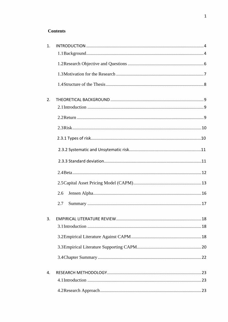
Contents

1. INTRODUCTION ...................................................................................................... 4

1.1 Background ...................................................................................................... 4

1.2 Research Objective and Questions .................................................................. 6

1.3 Motivation for the Research ............................................................................ 7

1.4 Structure of the Thesis ..................................................................................... 8

2. THEORETICAL BACKGROUND ................................................................................. 9

2.1 Introduction ..................................................................................................... 9

2.2 Return .............................................................................................................. 9

2.3 Risk ................................................................................................................ 10

2.3.1 Types of risk...............................................................................................10

2.3.2 Systematic and Unsytematic risk..............................................................11

2.3.3 Standard deviation....................................................................................11

2.4 Beta ................................................................................................................ 12

2.5 Capital Asset Pricing Model (CAPM) ........................................................... 13

2.6 Jensen Alpha .............................................................................................. 16

2.7 Summary ................................................................................................... 17

3. EMPIRICAL LITERATURE REVIEW .......................................................................... 18

3.1 Introduction ................................................................................................... 18

3.2 Empirical Literature Against CAPM ............................................................. 18

3.3 Empirical Literature Supporting CAPM ........................................................ 20

3.4 Chapter Summary .......................................................................................... 22

4. RESEARCH METHODOLOGY .................................................................................. 23

4.1 Introduction ................................................................................................... 23

4.2 Research Approach ........................................................................................ 23

2

4.3 Context of study ........................................................................................... 24

4.4 Sampling and Data Collection.......................................................................27

4.5 Variables .................................................................................................... 28

4.6 Data Analysis ............................................................................................ 31

4.6.1 Time series regression...............................................................................31

4.6.2 Cross-Sectional Regression .................................................................... 32

4.6.3 t-Test for Difference in Means ............................................................... 34

5. FINDINGS .............................................................................................................. 35

5.1 Introduction ................................................................................................... 35

5.2 Descriptive Statistics ..................................................................................... 35

5.3 Nature and Extent or Risk ............................................................................. 36

5.4 Jensen Alpha .................................................................................................. 37

5.5 Findings of t-tests .......................................................................................... 37

5.6 Cross-Sectional Regression: Relationship between Risk and Return ........... 38

5.6.1 Expected Return and Beta ...................................................................... 38

5.6.2 Expected Return, Beta, and Residual Variance ...................................... 40

5.7 Chapter Summary .......................................................................................... 41

6. CONCLUSION AND RECOMMENDATION .............................................................. 42

6.1 Conclusion .................................................................................................... 42

6.3 Summary and Discussion..............................................................................43

6.3 Limitations of the Study ................................................................................ 45

6.4 Recommendations for Future Research ........................................................ 45

7.REFERENCES .................................................................................................... 47

Appendix

Appendix 1. Information on Swedish Companies.......................................................53

Appendix 2. Information on Danish Companies.........................................................56

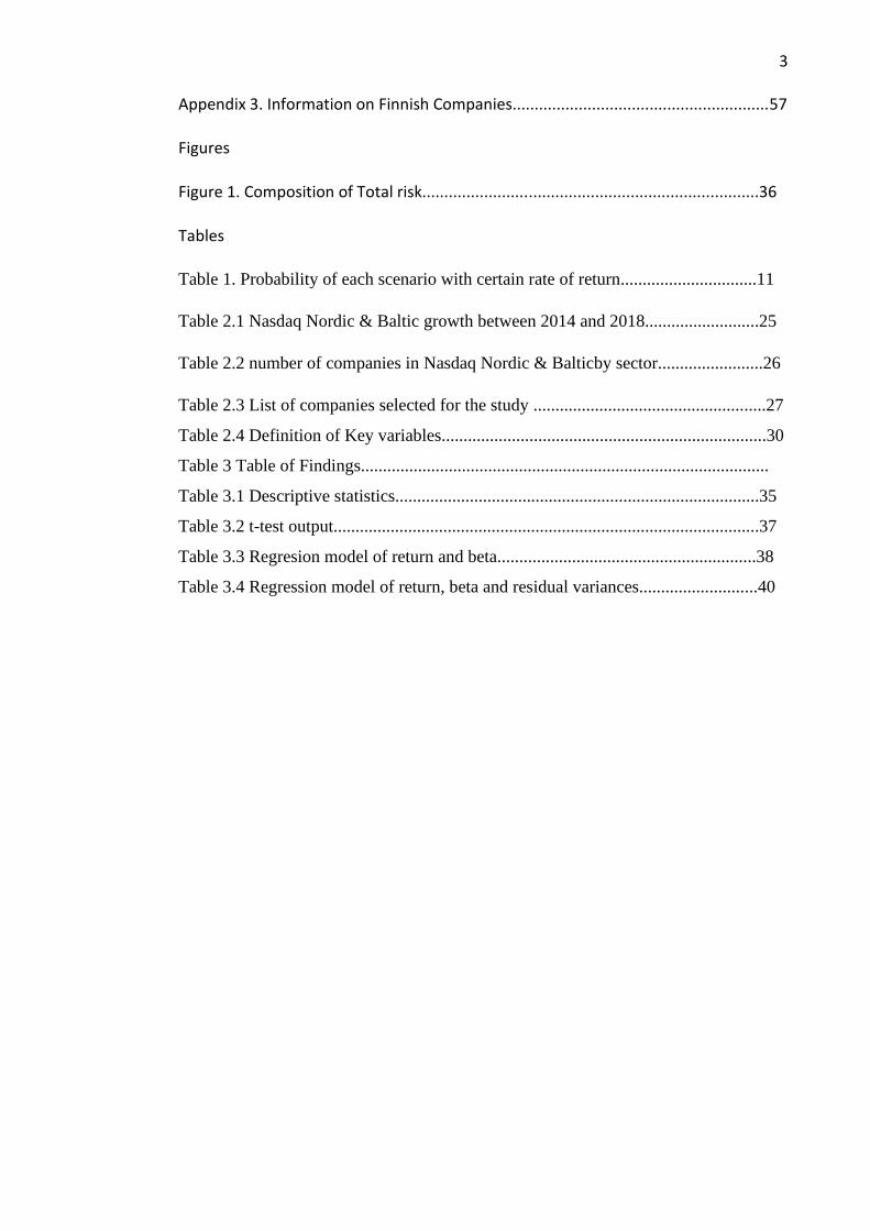
3

Appendix 3. Information on Finnish Companies..........................................................57

Figures

Figure 1. Composition of Total risk............................................................................36

Tables

Table 1. Probability of each scenario with certain rate of return...............................11

Table 2.1 Nasdaq Nordic & Baltic growth between 2014 and 2018..........................25

Table 2.2 number of companies in Nasdaq Nordic & Balticby sector........................26

Table 2.3 List of companies selected for the study .....................................................27

Table 2.4 Definition of Key variables..........................................................................30

Table 3 Table of Findings.............................................................................................

Table 3.1 Descriptive statistics...................................................................................35

Table 3.2 t-test output.................................................................................................37

Table 3.3 Regresion model of return and beta...........................................................38

Table 3.4 Regression model of return, beta and residual variances...........................40

4

1. INTRODUCTION

Capital Asset Pricing Model (CAPM) is one of the most significant concepts in

finance. The model argues that the required return on asset is influenced by its

systematic risk. The model is applied in estimating returns on assets, including

stocks. However, several researchers have argued that the CAPM does not

hold in stock markets. This thesis examines the relationship between risk and

return of Nordic stocks, thereby assessing the validity of the CAPM in the

Nordic Stock Market. It analyses the returns on 35 stocks to determine whether

the Nordic Stock Market has underperformed or outperformed, based on the

CAPM expected returns. It also tests whether systematic risk of Nordic stocks

has changed between 2009 and 2019.

1.1 Background

The primary motivation for most investors is making a return on their

investments. Nearly everything an investor doesin relation to their investment

is geared towards ensuring that an investment that is making profits continues

to make the same profit at the very least, and if possible, that the investment

starts to make even more profit. By the same token, investors are as well likely

to divest away from an investment if it is only returning losses with no

potential for profit. While, it is clear what investors hope for, the reality is that

some investors still make losses sometimes, even if this is not what they hoped

for. Markowitz (2016) argues that his happens because of the challenges

associated with making predictions about future profits. While technologies,

historical financial data analysis skills, and investment models can be used to

predict the behavior of stocks, the risks of losses cannot be eliminated entirely.

Thus, investors always have to accept some level of risk when making their

investments.

The question therefore shifts from whether the investor can eliminate all risks

while making investment decisions, to how the investors can manage the risks

associated with their investments.

By shifting the question, the focus therefore turns to the relationship between

risk and return, a concept that has been examined at length by both scholars

5

and investors. Brealey, Myers and Allen (2011) rightly points out that risk-

return relationship is one of the most significant aspects considered in various

investment decisions. According to Gitman, Joehnk & Smart (2015), the risk

associated with an investment determines the investor’s expected return,

whereby the higher the risk, the more chances are of a higher return. This is

the basis of the tradeoff theory, and what this means for investors is that they

always have to choose between the two conflicting goals: minimizing risk

ormaximising returns. Brigham & Houston (2016) further notes that most

investment managers know this, and for that reason, they employ the use of

various models to help predict the estimated risks and the expected returns of

their portfolio. One popularly used model is the capital asset pricing model

(CAPM).

The CAPM is applied in determining the relationship between risk and return

on an investment. According to Watson and Head (2016), unsystematic risk is

ignored in portfolio management and other investment decisions, since it can

be eliminated through diversification. The concept of CAPM is also applied in

estimating the cost of capital, which is used in investment appraisal decisions.

This is vital in assessing the viability of projects using the net present value

(NPV) criterion. Long-term investments such as purchase of fixed assets,

expansion, and introduction of new products, among others are appraised using

NPV. The NPV discounts all the expected cash flows at the company’s cost of

capital.

The CAPM lays the foundation for the relationship between risk and return

(Brealay, Myers, and Allen 2011). It argues that investors are risk-averse and

require a higher return on an asset associated with a high risk. It implies that if

an investment has a high risk, it must generate a high return to attract

investors. The CAPM posits that risk can be divided into systematic and

unsystematic risk. Systematic risk relates to market-wide factors and cannot be

eliminated by diversification, while unsystematic risk is due to firm and

industry-specific factors. Systematic risk is measured by beta, which measures

an asset’s risk relative to the market risk. The model assumes that investors

can eliminate all the unsystematic risk by establishing well-diversified

portfolios. Therefore, they base their investment decisions solely on systematic

6

risk. The model is widely used in estimating required returns on stocks and

other investments. This thesis investigates the relationship between risk and

return of Nordic stocks to assess the validity of the CAPM. It also uses the

CAPM to compare the performance of the Nordic stocks with the CAPM’s

estimated required returns.

Despite is usefulness, questions have emerged regarding the usefulness of

CAPM to predict the relationship between risk and return, with some

researchers concluding that it does not offer any meaningful estimations of risk

and return. The CAPM assumes that returns on an investment depend on the

investment’s systematic risk since unsystematic risk is irrelevant in investment

decisions. However, various researchers have questioned the validity of

CAPM and challenged its application in pricing assets. For instance, Dempsey

(2013) argues that the empirical evidence against CAPM is so compelling that

the model should be abandoned. Östermark (1991) also found evidence against

the validity of CAPM in the Finish and Swedish stock markets. The conflicting

findings in the various studies that exist so far make it a challenge for

managers and investors to know whether CAPM can benefit them or not.

Beyond the conflicting findings, fewstudies discuss the significance of CAPM

within the Nordic Stock Market, which lead to information gap. This

background show why a furtherstudy of CAPM and its usefulness in the

Nordic Stock Market is important.

1.2 Research Objective and Questions

The goal of this research is to determine whether CAPM beta (systematic) and

total risk explain the cross-section variation in returns on stocks listed on the

Nordic Stock Market. To achieve this goal, the following research questions

have been deduced:

i. What is the nature and extent of risk in the last 10 years?

ii. Has the Nordic stock market underperformed or outperformed the

expected return (CAPM) in the last 10 years?

iii. Is there any change in systematic, unsystematic and total risks in

Nordic stock market in the last 10 years between 2009 and 2019?

7

iv. What is the relationship between risk and return of stocks listed on

the Nordic Stock market?

In the first question, CAPM is used to estimate beta and calculate systematic

risk. This will help determine the proportion of total risk (standard deviation)

that is accounted for by systematic and unsystematic risks. For the second

question, Jensen alpha is used to determine the difference between the actual

returns on the stocks and the estimated required returns (CAPM returns).

Studying the relationship between risk and return helps determine whether the

CAPM is valid or not.

1.3 Motivation for the Research

This study is motivated by two reasons, one being a practical justification, and

the second being a theoretical justification. The theoretical justification is

inspired by the gaps observed in the extent studies as shown in the

background. As it is, a number of studies have shown that CAPM can be used

to help in estimating risk and return. At the same time, contrasting studies have

shown that CAPM is not a sufficient approach to estimate risk and return.

Thus, by making an additional study, a review of extant literature is made,

which critically examines the findings of previous studies and makes a critical

review why CAPM is considered inadequate. The study also presents an

updated review of literature, which is far from the authority in the subject, but

provides a relevant additional information to both researchers and students of

finance management. However, CAPM is a major area of finance which helps

investors to know the risk and return. According to ACCA (2019), CAPM was

published by William Sharpe in the year 1986. Watson & Head (2016) states

that unsystematic risk can be ignored but systematic risk plays a very

important role.

Secondly, on a practical level, the resulting controversy on the significance of

CAPM makes it harder for managers to make decisions on whether they will

adopt the model when making their investment decisions. This thesis may

contribute to the knowledge necessary in making investment decisions as it

focuses specifically on the relationship between risk and return on Nordic

stocks to assess the validity of data. The research determines whether CAPM

8

beta is a significant determinant of the variations in cross-section returns of the

Nordic stocks using more recent data from 2009 to 2019. The findings of this

thesis can help investors and companies listed on the stock markets of Finland,

Denmark and Sweden to better understand the relationship between risk and

return.

1.4 Structure of the Thesis

The study is organized into six different chapters. Chapter one discusses the

background, aims, and objectives, as well as the justification for studying the

CAPM in the Nordic Stock Market. Chapter two reviews theoretical

background of CAPM, including its assumptions and its limitations. Chapter

three reviews empirical studies on the CAPM and relationship between risk

and return, identifying gaps in research. Chapter four of the study explains the

research methodology, including a description of the data used and how it is

collected, as well as a discussion of the statistical methods applied. The

chapter also includes a justification for the models used. Chapter five presents

the findings of data analysis, implications of the findings, and links to findings

to existing empirical studies. Finally, Chapter six is conclusion of the study,

including a summary of the research, limitations of the study, and areas for

further research.

9

2. THEORETICAL BACKGROUND

2.1 Introduction

This chapter discusses the theoretical literature on CAPM and the relationship

between risk and return. The first section, theoretical background, defines

return, risk, CAPM, expected return and Jensen alpha. The section also

highlights the different types of risk, as well as measures for risk and return.

2.2 Return

Brealey, Myers and Allen (2011) define return as the profit or loss on any

investment activity. Return includes profit, interest, or dividend earned on an

investment, plus capital gains (Watson & Head, 2016). Capital gain or loss

refers to the change in the value of the investment over a period. Mayo (2012)

identifies three types of return; realized, expected, and required returns.

Realized return is the measure of how much an investor has gained or lost on

an investment over the period the investment was held. The realized return on

a stock is calculated as follows:

Realized return = (Ending Price−Initial Price)+Dividends

Initial Price × 100%

Expected return is the gain or loss an investor anticipates from an investment,

based on its historical performance (Mayo 2012). For instance, the expected

return on a stock is the historical average return of the return. Under

uncertainty, the expected return is calculated as follows:

Expected return =∑ 𝑅𝑖𝑃𝑖, where Ri is the return and Pi is the probability of the

condition.

Required return is the minimum return expected on an investment. It is the

opportunity cost of capital, that is, the amount an investor would earn on other

available market securities. According to Gittman and Zutter (2015), a rational

investor cannot commit on an investment if its expected return is lower than

the required return. In efficient markets, the expected return is equal to the

required return (Ilmanen 2012).

10

2.3 Risk

According to Yang (2014), the risk which is involved in an investment can

indirectly explained with some specific concepts.

2.3.1 Types of Risk

Risk- Here, in the case of investment, the return always remains uncertain

because nobody knows the situation of market as well as what will be the

situation in the future so there is always some risk involved in every kind of

investment. So, risk is all about the uncertainity available in the expected

return. Taking risk may lead to an opportunity as well as loss because no one

knows what will happen next. Accordingly, every investment involves risk

(Bodie et al. 2004).

Risk free- Risk free is a type of return in which investors get some return by

the end of their holding period. Here, government bond is also taken as risk

free assets due to the fact that government always print money and this is

helpful for the investors as they get assured about their investment. Investors

need to give some amount in advance so that they will get that amount back at

the end of period (Sibilkov 2007).

Risk premium- Risk premium is all about the compensation involved in the

investment. This can be measured by the rate of return earned by having the

investment from the excess of risk free ROR (Drobny 2010).

Therefore, risk refers to the variability or volatility of returns associated with

an investment (Markowitz 2016). Due to changes in the firm’s operating

conditions, sector and market factors, an investment may not generate the

expected return (Markowitz 2016). Therefore, investment decisions must

consider both expected returns and risk.

The total risk associated with an investment is measured using the standard

deviation. Standard deviation is measure of the variability of returns from the

mean return (Watson & Head 2016). It is determined by getting the square of

variance as follows:

Var(r) =∑ (𝑟𝑖 − 𝜇)2𝑛1 , where ri is the return and μ is the mean or average return.

Standard deviation = √𝑉𝑎𝑟(𝑟)

11

2.3.2 Systematic and Unsystematic return

According to Markowitz (2016), total risk is divided into systematic and

unsystematic risk, depending on the contributing factors.

Total Risk = Systematic Risk + Unsystematic Risk

Unsystematic risk: It the risk inherent in a specific firm or industry(Moyer,

McGuigan & Kretlow 2005). It is due to factors such as employee strikes,

government policy specific to a sector, firm’s financial challenges, and

unavailability of raw materials, among other firm-specific factors. It is also

called diversifiable risk since it can be eliminated through diversification.

Systematic Risk: It is the proportion of total risk that is inherent in the entire

market. It is due to market-wide factors and affects all firms or investments

irrespective of the sector (Moyer et al. 2005). Causes of systematic risk include

changes in interest, inflation, exchange rates, among other market-wide factors

(Moyer, et al. 2005). Such factors are beyond the control of a firm or investor.

Thus, unsystematic risk cannot be eliminated through diversification (Watson

& Head 2016). According to Markowitz (2016), unsystematic risk can be

eliminated through diversification, hence investors base their decisions on

systematic risk. Systematic risk is measured using beta.

2.3.3 Standard deviation- A Measure of Risk

Bodie at al. (2004) discussed that while making a decision to invest or not, an

investor has to take the possible outcomes of investing in current scenario and

also HRP stocks in the current scenario. After that, he also needs to caculate

the estimated probability of every scenario.

Table 1- Probability of each scenario with certain rate of return [Accessed

from Bodie at al. (2004)]

12

Here, an example is taken in the above table where s denotes the number of

scenario. The statistical measurement of expected risk and return is presented

in the above table of probability distribution. According to the table, HRP is

equal to the return on the investment which is expected.

E(Rt)=RtPs where,

Rt denotes realized return of every single stock.

Variance is used to measure the volatility of the realized return. This is helpful

in calculating or estimating the uncertainty of the risk. In addition to that, we

take square root of variance for calculating the standard deviation so that the

risk taken from expected return must have the same dimensions.

However, for calculating the stock performances, standard deviation and the

expected return are the major parameters (ibid).

2.4 Beta

Beta is a measure of an investment’s volatility relative to that of the entire

market (Lumby & Jones 2003). For instance, if a stock’s beta is 1.2, it implies

that the volatility of the stick’s returns is 20% greater than that of the market.

On the other hand, a beta of 0.8 implies that the stock’s risk is 20% lower

than that of the market. This also implies that if the market volatility increases

by 1 unit, the stock’s risk will increase by 0.8 (Lumby & Jones 2003).

Beta is calculated by determining the covariance between the stock’s return

and the index or benchmark’s return divided by the variance of the

benchmark’s return (Lumby & Jones 2003). Alternatively, it be estimated by

getting the regression of a stock’s returns on the benchmark’s return (Lumby

& Jones 2003). It is the coefficient of the benchmark’s return in the regression

model.

13

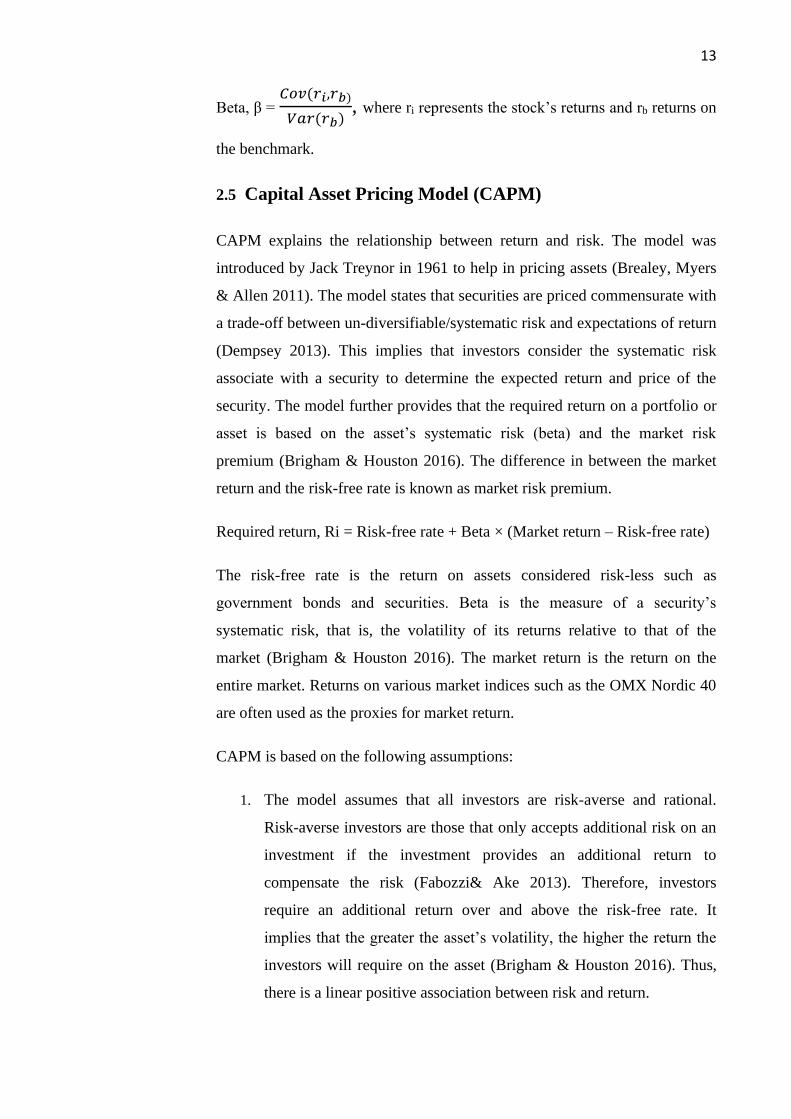
Beta, β = 𝐶𝑜𝑣(𝑟𝑖,𝑟𝑏)

𝑉𝑎𝑟(𝑟𝑏), where ri represents the stock’s returns and rb returns on

the benchmark.

2.5 Capital Asset Pricing Model (CAPM)

CAPM explains the relationship between return and risk. The model was

introduced by Jack Treynor in 1961 to help in pricing assets (Brealey, Myers

& Allen 2011). The model states that securities are priced commensurate with

a trade-off between un-diversifiable/systematic risk and expectations of return

(Dempsey 2013). This implies that investors consider the systematic risk

associate with a security to determine the expected return and price of the

security. The model further provides that the required return on a portfolio or

asset is based on the asset’s systematic risk (beta) and the market risk

premium (Brigham & Houston 2016). The difference in between the market

return and the risk-free rate is known as market risk premium.

Required return, Ri = Risk-free rate + Beta × (Market return – Risk-free rate)

The risk-free rate is the return on assets considered risk-less such as

government bonds and securities. Beta is the measure of a security’s

systematic risk, that is, the volatility of its returns relative to that of the

market (Brigham & Houston 2016). The market return is the return on the

entire market. Returns on various market indices such as the OMX Nordic 40

are often used as the proxies for market return.

CAPM is based on the following assumptions:

1. The model assumes that all investors are risk-averse and rational.

Risk-averse investors are those that only accepts additional risk on an

investment if the investment provides an additional return to

compensate the risk (Fabozzi& Ake 2013). Therefore, investors

require an additional return over and above the risk-free rate. It

implies that the greater the asset’s volatility, the higher the return the

investors will require on the asset (Brigham & Houston 2016). Thus,

there is a linear positive association between risk and return.

14

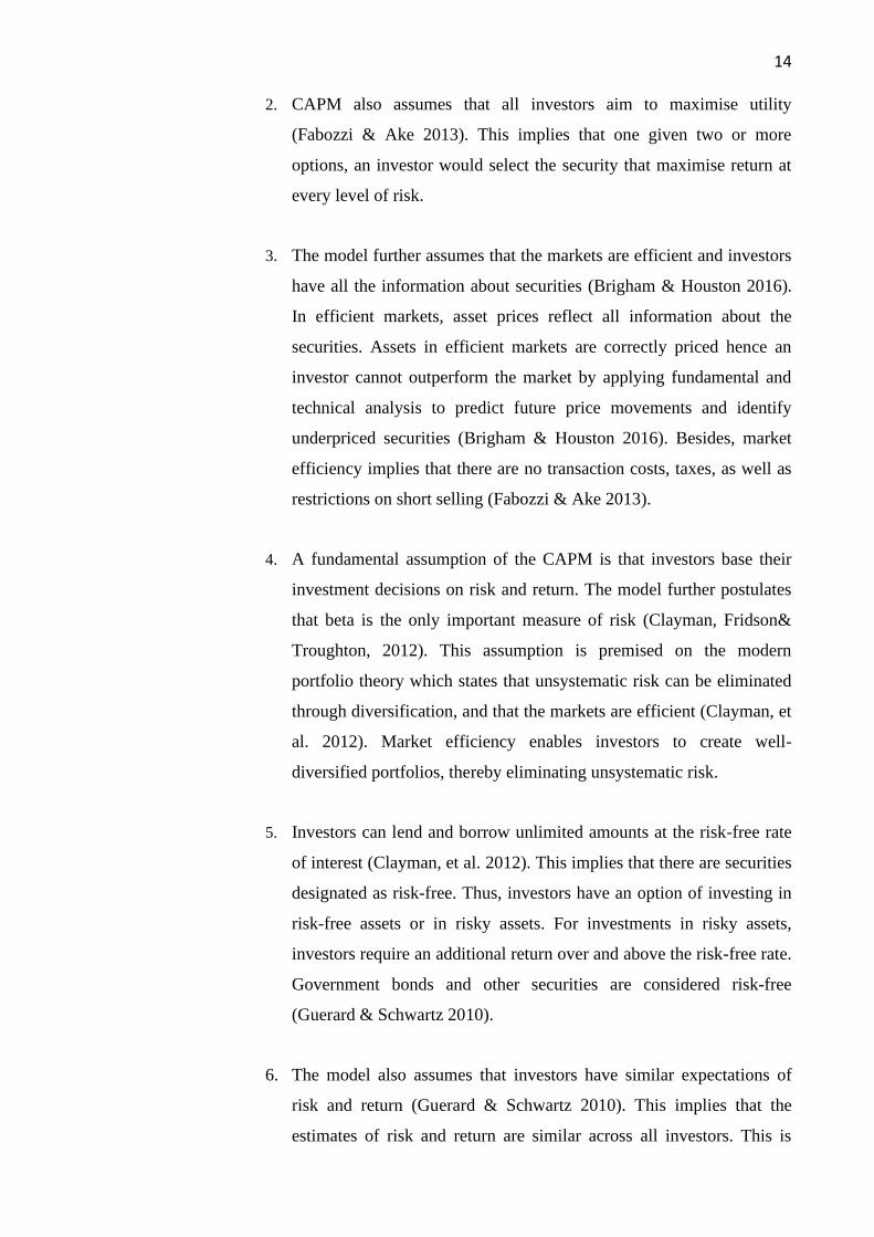
2. CAPM also assumes that all investors aim to maximise utility

(Fabozzi & Ake 2013). This implies that one given two or more

options, an investor would select the security that maximise return at

every level of risk.

3. The model further assumes that the markets are efficient and investors

have all the information about securities (Brigham & Houston 2016).

In efficient markets, asset prices reflect all information about the

securities. Assets in efficient markets are correctly priced hence an

investor cannot outperform the market by applying fundamental and

technical analysis to predict future price movements and identify

underpriced securities (Brigham & Houston 2016). Besides, market

efficiency implies that there are no transaction costs, taxes, as well as

restrictions on short selling (Fabozzi & Ake 2013).

4. A fundamental assumption of the CAPM is that investors base their

investment decisions on risk and return. The model further postulates

that beta is the only important measure of risk (Clayman, Fridson&

Troughton, 2012). This assumption is premised on the modern

portfolio theory which states that unsystematic risk can be eliminated

through diversification, and that the markets are efficient (Clayman, et

al. 2012). Market efficiency enables investors to create well-

diversified portfolios, thereby eliminating unsystematic risk.

5. Investors can lend and borrow unlimited amounts at the risk-free rate

of interest (Clayman, et al. 2012). This implies that there are securities

designated as risk-free. Thus, investors have an option of investing in

risk-free assets or in risky assets. For investments in risky assets,

investors require an additional return over and above the risk-free rate.

Government bonds and other securities are considered risk-free

(Guerard & Schwartz 2010).

6. The model also assumes that investors have similar expectations of

risk and return (Guerard & Schwartz 2010). This implies that the

estimates of risk and return are similar across all investors. This is

15

attributed to the fact that information is available to all investors in the

market (Clayman, et al. 2012). Therefore, all investors give a similar

estimate of the price of a security.

7. CAPM also assumes that investors have identical horizons

(Markowitz 2016). This implies that investors buy all securities and

sell them at one common point in time. Thus, the model assumes a

single investment horizon. This means that investors are only

concerned about the terminal wealth, that is, the value of the

investment at the end of the investment period.

8. Finally, the model assumes that all securities are marketable and

highly divisible (Markowitz 2016). This indicates that it is possible for

an investor to buy or sell any security at any time they wish.

The CAPM has been criticized for its theoretical limitations. According to

Brigham and Houston (2016), CAPM is based on unrealistic assumptions. For

instance, the assumption of a single period investment horizon is unrealistic.

Investors are not only concerned about the terminal value of their investments.

In reality, most investors have continuous investment horizons. Besides, the

assumption that all investors have similar expectations of risk and return is

unreasonable. Investors have different expectations of the market (Kurschner

2008). This is due to the fact that markets are not perfectly efficient.

Information is not available to all investors. This explains why some investors

outperform the market by incurring efforts and resources to obtain information

that is not readily available, through measures such as technical and

fundamental analysis (Peterson 2012). The assumption that investors can

borrow and lend unlimited amounts of money at the risk-free rate of interest is

also unrealistic (ibid.)

16

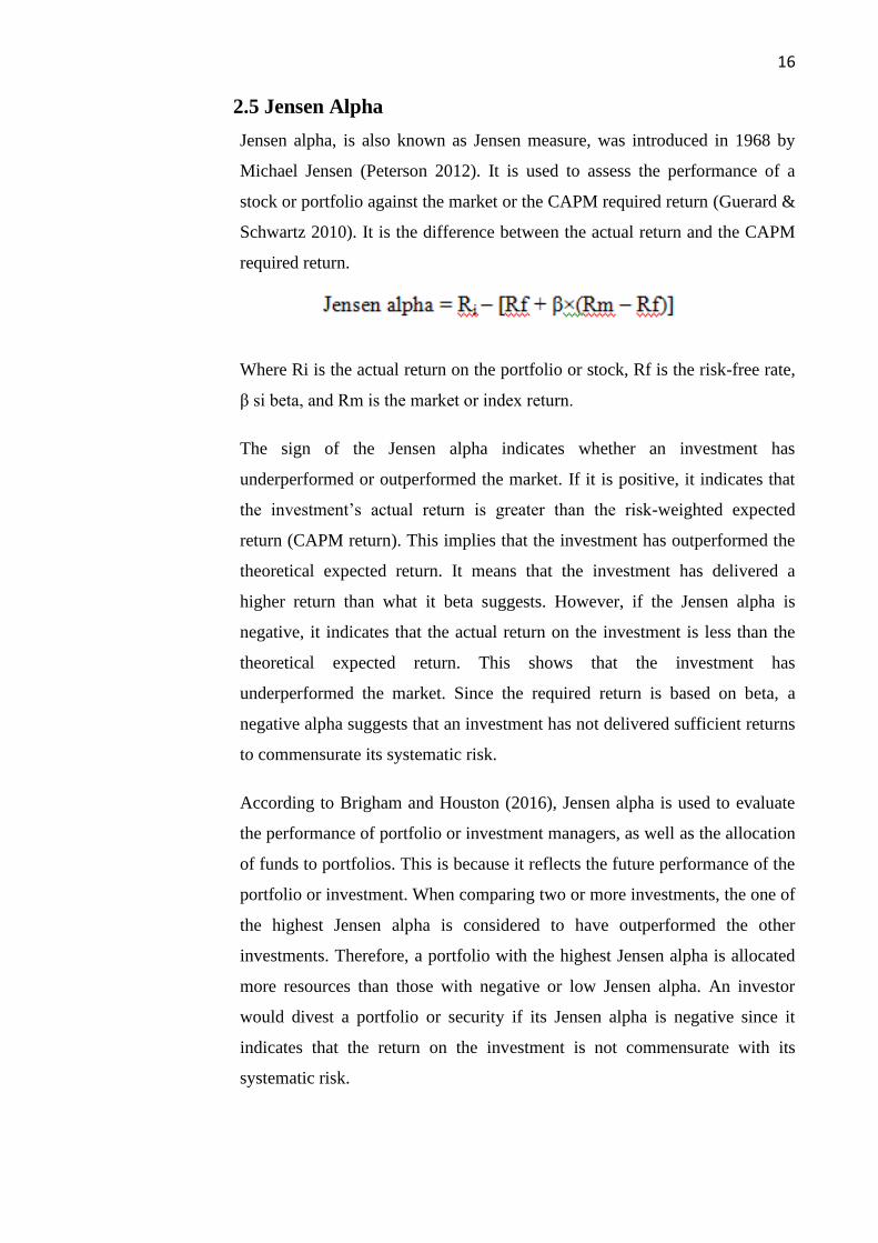
2.5 Jensen Alpha

Jensen alpha, is also known as Jensen measure, was introduced in 1968 by

Michael Jensen (Peterson 2012). It is used to assess the performance of a

stock or portfolio against the market or the CAPM required return (Guerard &

Schwartz 2010). It is the difference between the actual return and the CAPM

required return.

Where Ri is the actual return on the portfolio or stock, Rf is the risk-free rate,

β si beta, and Rm is the market or index return.

The sign of the Jensen alpha indicates whether an investment has

underperformed or outperformed the market. If it is positive, it indicates that

the investment’s actual return is greater than the risk-weighted expected

return (CAPM return). This implies that the investment has outperformed the

theoretical expected return. It means that the investment has delivered a

higher return than what it beta suggests. However, if the Jensen alpha is

negative, it indicates that the actual return on the investment is less than the

theoretical expected return. This shows that the investment has

underperformed the market. Since the required return is based on beta, a

negative alpha suggests that an investment has not delivered sufficient returns

to commensurate its systematic risk.

According to Brigham and Houston (2016), Jensen alpha is used to evaluate

the performance of portfolio or investment managers, as well as the allocation

of funds to portfolios. This is because it reflects the future performance of the

portfolio or investment. When comparing two or more investments, the one of

the highest Jensen alpha is considered to have outperformed the other

investments. Therefore, a portfolio with the highest Jensen alpha is allocated

more resources than those with negative or low Jensen alpha. An investor

would divest a portfolio or security if its Jensen alpha is negative since it

indicates that the return on the investment is not commensurate with its

systematic risk.

17

2.7 Summary

The chapter reviewed theoretical and empirical literature on CAPM and the

relationship between risk and return (Fabozzi& Ake 2013). Risk and return

are fundamental measures investors rely on during investment decisions. Risk

refers to the variability of returns on an investment (Brigham & Houston

2016). Risk is classified into systematic and unsystematic risk depending on

the contributing factors. Systematic risk is due to market-wide factors such as

changes in interest rates, inflation, and exchange rates, among other variables.

Unsystematic risk is due to firm and sector-specific factors (ibid.)

Unsystematic risk can be eliminated by creating a well-diversified portfolio of

assets. Systematic risk is measured using beta, while total risk is measured

using standard deviation. Because unsystematic risk can be eliminated,

CAPM assumes that beta is the only determinant of stock and portfolio

returns (Fabozzi& Ake 2013). Modern portfolio theory provides a guideline

for reducing portfolio risk. It recommends that investors should create a

portfolio consisting of unrelated stocks, since the covariance between such

stocks is low. The theory suggests that investors can create an efficient

portfolio, or the minimum variance portfolio. This is the portfolio that

maximizes the risk-adjusted performance (Brigham & Houston 2016). Risk-

adjusted measures include Sharpe and Treynor ratios. Sharpe ratio shows the

excess return above risk-free rate per unit of standard deviation (Fabozzi&

Ake 2013). The chapter also discussed CAPM including its assumptions such

as existence of risk-free rate, similar expectations of risk and return, markets

are efficient, among other assumptions.

18

3. EMPIRICAL LITERATURE REVIEW

3.1 Introduction

This section reviews the empirical literature on CAPM and the relationship

between risk and return. Empirical literature review is important since it

enhances understanding of the topic and enables the identification of research

gaps. It assists in developing hypothesis and determining the appropriate

methodology for future studies on CAPM.

After the introduction of CAPM, various empirical studies have been

conducted to determine its validity in stock markets. Most of the studies have

focused on one fundamental assumption of the CAPM, that is, beta is the only

determined of return, and that the relationship between beta and return is

linear. Based on this assumption, the regression model of return and beta

should be statistically significant. Besides, the intercept of the model should

not be significantly different from the risk-free rate.

3.2 Empirical Literature Against CAPM

Among the early empirical studies on the CAPM was conducted by Lintner.

Lintner used ten-year data on 301 stocks from 1954 to 1963. Lintner’s

analysis involved a two-stage regression analysis. The first stage was the time

series regression analysis conducted to estimate the beta of each asset. The

slope of the regression of the stock’s returns and the market returns gave an

estimate of beta. The second stage of the analysis involved a cross-section

regression of the 301 pairs of returns and beta. Lintner’s cross-sectional

regression model is shown by the following equation:

Ri = α0 + α1β + є

Lintner found that the intercept of the cross-sectional regression was

significantly different (greater) than the risk-free rate. Besides, the coefficient

of beta in the model was not statistically significant. Lintner concluded that the

analysis did not support the validity of CAPM.

Miller, Jensen, and Scholes (1972) analysed monthly data of all securities

listed on the NYSE from January 1926 to December 1930. They used time-

19

series regression to estimate beta for each of the stocks. They then divided the

sample into ten different portfolios based on beta values. Miller, et al. (1972)

then conducted two cross-sectional regressions. The first cross-section

regression was between portfolio returns and beta. In the second regression,

Miller, et al. (1972) added residual variance to the model. The results showed

that the R-square of the model increased when residual variance was added.

This indicates that beta is not the only determined of return, thereby

invalidating CAPM.

Levy (1978) used the same methodology as Miller, et al. (1972) analyzing

twenty-year data of 101 stocks. The r square of the model cross-sectional

regression with beta was 0.21, but when variance was added, the r-square

increased to 0.38. Levy (1978) concluded that the CAPM was not valid since

beta was not the only determined of return on stocks and portfolios. Fama and

French (2003) also tested the empirical validity of the CAPM and found no

empirical proof of CAPM assumptions.

Novak, and Petr (2004) studied the impact of CAPM beta, market value of

equity and momentum on stock return on the Stockholm Stock Exchange. The

study found that none of the factors, including CAPM beta is significant for

explaining stock returns on the Stockholm Stock Exchange. This suggests that

CAPM is not valid since it posits that CAPM beta is a significant and the only

factor explaining variability of stock returns.

Östermark (1991) used regression model to assess the relationship between

beta and stock returns in two Scandinavian Stock Markets; Sweden and

Finland. The study relied on the r-square (coefficient of determination) to

assess the explanatory power of squared beta. The study found that in the

Finnish Stock Market, the explanatory power of squared beta was low. The

model for the Swedish Stock market indicates that squared beta explained a

greater percentage of the variations in stock returns than in the Finnish market.

Östermark (1991) concluded that the Finnish model was consistent with

international evidence on the invalidity of CAPM.

Boďa and Kanderová (2014) used monthly data of 10 S&P 500 index stocks

from 2003 to 2012 to test the linearity of the relationship between CAPM beta

20

and stock returns. They divided the data into two subsequent non-overlapping

5-year sub periods. They used regression model to determine the relationship

between beta and stock returns. The study found that there is no linear

relationship between beta and stock returns. Besides, there was a significant

change in beta between the two sub periods. The results invalidate the linearity

assumption of CAPM (Boďa, and Kanderová 2014).

Anwar and Kumar (2018) tested whether the CAPM holds in the Indian stock

market, using data of NIFTY 50 companies from April 1, 2009 to March 31,

2016. The performed time-series regression to determine stocks’ betas and

cross-sectional regression to assess the relationship between beta and stock

returns. The data was subcategorized into portfolios based on size and value.

The regression models indicated that CAPM beta was not robust in explaining

stock returns of the NIFTY 50 companies. However, when portfolios were

used, the explanatory power of the CAPM beta improved although it was still

very low. Anwar and Kumar (2018) concluded that the CAPM did not hold in

the Indian stock market.

Karp and Van Vuuren (2017) studied the validity of CAPM and the Fama

French Three-Factor model in the Johannesburg Stock Exchange. Using data

of 46 companies listed on the JSE from 2010 to 2015, they constructed

portfolios using an annual sorting procedurebased on Size and Book-to-

Market. The study found that the models are poor in explaining stock returns.

However, Karp and Van Vuuren (2017) identified inadequate market proxy

measures as the primary reason for the poor performance of the models.

These findings suggest that CAPM is inadequate in being used as a proxy to

help improve returns to investors. Particularly, the studies looked at how the

model influences beta, stock’s returns and the market returnin various

marketsacross selected stock exchanges. They find that CAPM is not robust

enough to explain the returns earned, irrespective of the company or market in

question.

3.3 Empirical Literature Supporting CAPM

Although most studies have rejected the validity of CAPM, other studies have

supported the validity of CAPM and its application in estimating stocks’

21

returns. Fama and MacBeth (1973) studied monthly percentage returns of all

stocks listed on the New York Stock Exchange between January 1926 and

June 1968. They performed time-series regression on each stock to estimate

betas. They divided the data into 20 portfolios on the basis of ranked betas of

individual stocks, with each portfolio having equally weighted stocks. They

estimated the beta for each portfolio (equally weighted), residual variance and

squared beta. Fama and MacBeth (1973) then conducted cross-sectional

regression analysis with actual returns on each portfolio as the dependent

variable, while beta, residual variance and squared beta were the independent

variables. Analysis showed the intercept of the model was not statistically

significant. The coefficients of squared beta and residual variance were not

statistically significant, while the coefficient of beta was statistically

significant. They concluded that the regression showed that beta was the only

significant determinant of stock returns, thereby supporting the CAPM.

Sreenu (2018) tested the capital asset-pricing model (CAPM) and three-factor

model of Fama in Indian Stock Exchange. Using daily and annual average data

of 54 companies listed on the National Stock Exchange from 2010 to 2016,

they developed regression models for both the CAPM and Fama models. The

results showed that the intercepts of both models were statistically

insignificant (Sreenu 2018). This supports CAPM since an insignificant

coefficient implies that beta is the only factor explaining variability of returns.

Satrio (2015) tested the validity of CAPM and the Three-Factor model in

explaining returns of Indonesian stocks. Using data of 284 firms listed on the

Indonesian Stock Exchange from December 2002 to December 2012, he found

that CAPM is valid.

Roll (1977) provided a critique of the empirical tests that concluded that

CAPM is not valid and should not be applied in estimating returns. He argued

that the so called ‘empirical tests’ are invalid since they are based on

inefficient benchmarks. When estimating beta of a portfolio or stock, the

returns are regressed against the returns on a benchmark or market index.

CAPM requires such benchmark to be efficient. Roll (1977) also argued that

empirical arguments against CAPM are not valid from the theoretical and

practitioner’s view point. The fundamental principle of the CAPM is that

22

investors only consider systematic risk when determining returns since they

can eliminate unsystematic risk through diversification (Roll 1977). The

critique of CAPM that beta is not the only risk determining returns implies that

investors expected to be paid or compensated for unavoidable risk, an idea

which Roll (1977) finds inconsistent with the beliefs of theorists and

practitioners.

3.4 Chapter Summary

This chapter reviewed empirical studies that have been conducted to test

CAPM in stock markets. Most of these studies focused on the CAPM

assumption that beta is the only determinant of return. Empirical studies have

reached conflicting conclusions about the validity of CAPM in stock markets.

Miller, Jensen, and Scholes (1972), Levy (1978), and Boďa and Kanderová

(2014), among other studies found that CAPM does not hold in stock markets.

However, Fama, and MacBeth (1973), Sreenu (2018), and Satrio (2015) found

that CAPM is valid. The literature review shows that very few studies have

been conducted to test the validity of the CAPM in the Nordic Stock market.

This study uses the most recent 10-years data to test CAPM in the Nordic

stock market.

23

4. RESEARCH METHODOLOGY

4.1 Introduction

This chapter explains the research approach and strategy, data collection

method and variables used in the study. It also explains the statistical methods

employed to determine the relationship between risk and return, and test

CAPM.

4.2 Research Approach

Various research approaches can be used to conduct a study, and according to

one if the researcher, the choice of a particular approach over the other is

often pegged on how the researcher indents to treat truth and objectivity,

collect data, ananlyse the data and make inferences from the study. The

question of truth and how it is treated in a research is determined by the

research philosophy, of which there are positivism and interpretivism. On

research philosophy, this thesis is a positivism study. According to Wilson

(2019), a positivist research approach is a study in which the researcher is

independent and the findings can be considered objective. In this case, the role

of the researcher is restricted to collecting data and interpreting the results of

data analysis. The data used in the analysis is secondary data (stock prices),

which the researcher has no control over. The main strength of a positivist

approach over interpretivism is that it maintains objectivity where

interpretivists treat data with a subjective view, thereby leading to research

biases.

Trochim (2005) outlines two types of logical reasoning in research: inductive

and deductive. The key differences between them is that inductive techniques

focus on generating new theory and thought, whereas deductive reasoning

focus on testing the existing thought or theory to see its applicability within a

given context.A deductive approach implies that the aim of the study is to test

hypothesis about existing theories and not to develop new theories (Trochim

2005). The study adopts a deductive approach for two reasons. First, as

outlined in chapter one, this study aims at finding out whether CAPM beta

(systematic) and total risk explain the cross-section variation in returns on

stocks listed on the Nordic Stock Market. CAPM is an existing theory, which

means the use of a deductive approach to examine it is appropriate. Secondly,

24

this study focuses on a specific context, rather than just examining the theory

in a broad spectrum. Particularly, in this case, the hypothesis tested is whether

CAPM is valid in the Nordic Stock Exchange.

Another important methodological consideration was the research strategy.

According to Mc Burney and White (2013), research strategies can be

categorized into many brackets, the main ones being case studies, surveys,

experiments and field excursions. In the present case, case study is the

preferred strategy. Case studies refer to a research in which the goal is to look

at a specific organisation, country or segment of the market with the goal of

understanding how a phenomenon influences that selected entity based on its

unique characteristics. The strengths of conducting a case study is that the

findings are often specific to the context, making it relevant for

recommendations to be drawn and implemented from them. He also points out

that using a case study approach limits the ability to generalize findings.

Nevertheless, by using the case study approach, this study can focus

particularly on the Nordic stock market, which is where the research interest is

situated (ibid.)

Finally, this thesis uses a correlational research design. According to Mc

Burney and White (2013), a correlational research design involves determining

the relationship between two variables using quantitative data. The variables in

this study are numerical, making it possible to conduct a correlational

(quantitative) research.

4.3 Context of the study

As mentioned, the study is based on the Nordic stock markets. Before

describing the sampling and data collection procedures, it is imperative to

situate the study within the context. Nordic countries refer to countries situated

within a specific geographical region of North Atlantic and Northern Europe,

and typically comprise Sweden, Norway, Iceland, Denmark, Finland,

Greenland and Faroe Islands (Gotz 2003).The financial services and

marketplaces for this region is controlled by the Nasdaq subsidiary, Nasdaq

Nordic, which also controls the Baltic and the Caucasian regions.

25

Nasdaq Nordic was formed in 2003 as OMX AB, when HEX plc merged with

OM AB. It was renamed to Nasdaq AB, although it is also known as OMX AB

since February 2008 (Bakie 2014). Nasdaq Nordicoperates two divisions,

which control eight exchanges. These include Copenhagen, Stockholm,

Helsinki, Iceland, Tallinn, Riga, Vilnius, and Armenian stock exchanges. It is

one of the larger Nasdaq subsidiaries in Europe based on key statistics.

Specifically, as of end of year 2018, the daily average traded in Nasdaq Nordic

was 3.10 billion EUR.

The stock market has seen growth across most of its indicators. According to

its annual trading statistics report, average trades per day grew by 13.4% in

2018, while derivatives grew by 4%. However, the number of new companies

listed in Nasdaq Nordic declined significantly, from 118 to 84 between 2017

and 2018, although this is due to switches of where some 23 companies were

listed during the period (Nasdaq Nordic 2019).Nevertheless, the total number

of listed companies in the Nasdaq Nordic continued to grow, jumping from

792 to 10002 between 2014 and 2019. Table 2.1 is a summary of the growth in

number of listed companies in the Nasdaq Nordic and Baltic as reported by

Nasdaq, while Table 2.2 is a summary of the main sectors within the market,

together with the number of companies represented for each market.

Table 2. 1: Nasdaq Nordic & Baltic growth between 2014 and 2018

Year end Total Number of Listed Companies

2014 792

2015 852

2016 900

2017 984

2018 1,002

26

Table 2.2. number of companies in Nasdaq Nordic & Balticby sector

Industry/ sector Companies per ICB Sector

Oil & Gas 27

Basic Materials 47

Industrials 238

Consumer Goods 113

Health Care 149

Consumer Services 102

Telecommunications 15

Utilities 13

Financials 178

Technology 120

Total 1002

Notably as well, one of the main indices for the Nasdaq Nordic is the OMX

Nordic 40 (OMXN40), which was formed in 2006. The index consists of 40

most traded stock classes under the OMX Nordic umbrella in four markets,

which are Stockholm, Reykjavik, Helsinki and Copenhagen.

This context is significant for the study because Nasdaq Nordic is one of only

two pan-European stock exchanges active today. Further, it is larger than the

fellow Euronext by number of European markets represented in the listings.

By using Nasdaq Nordic, the study is able to find the most reliable data for the

selected study objective.

27

4.4 Sampling and Data Collection

According to Silverman (2010), it is advisable to work with a representative

sample where the population being studied is too large to be used in its

entirety. The context discussed above comprised more than a thousand

companies, which is too large for the scope of this study. This calls for

sampling techniques that are both useful and suitable for the particular study

based on factors such affordability, timeliness, efficiency as well as relevance.

In this case, random sampling is found to be the most suitable. Yin (2003)

defines random sampling as the procedure for selecting participants in a study

whereby any sample is selected purely based on chance, and the probability for

selecting a sample is equal for all the samples.

A random sample of 35 companies was selected from the list of companies

traded on the Nordic stock markets; Finland, Denmark and Sweden. A random

sample is beneficial in research since it eliminates sampling bias that affects

the objectivity of the findings. Close market prices of each of the 35 selected

companies and the OMX Nordic 40 Index were collected for the ten years

between 1 April 2009 and 31 March 2019. The daily stock prices were

collected since the variable is critical in the determination of stocks’ returns, a

key variable in this analysis. All the data was obtained from the OMX Nordic

website.

Table 2.3 shows the selected companies and the countries from which they are

selected. In summary, six companies were from Finland, eight were from

Denmark, and 21 were from Sweden.

Table 2.3: List of companies selected for the study as follows-

Company name Country Total per country

ABB LTD

Alfa

ASSA Abloy

Atlas copco A

Astra zeneca

Boliden

Electrolux B

Ericsson B

Sweden 21

28

Hexagon B

H&M

Investor B

Nordea bank

Sandvik

SEB A SV.Handelsbanken A

SKF

Swedbank A

Swedish Match

Tele 2 B

Telia company

Volvo B

Carlsberg B

Danske bank

DSV

Genman

Novo nordisk B

Novozymes B Vestas wind system

Coloplast B

Denmark 8

Fortum oyj

Kone oyj

Neste oyj

Sampo oyj

Storaensooyj

UPM

Finland 6

4.5 Variables

The key variables used in the analysis include risk-free rate, average annual

return, standard deviation of returns (Total risk), beta, unsystematic risk,

CAPM return, and Jensen alpha.

29

4.5.1 Risk-Free Rate

This is the return on riskless assets. The risk-free rate is important in this

study since it is used in the determination of CAPM required rate of return.

The yield of government bonds represent the risk-free rate. In this study, the

yield on 10-year Finland government bond is taken as the proxy for risk-free

rate. As on 27 October, the yield on 10-year bond was 0.138% (World

Government Bonds 2019). The annualized risk-free rate is determined as

follows:

Annualized Rf = (1 + 0.138%)250 - 1 = 3.51%

4.5.2 Return

Return is the percentage change in the daily close price of a stock. Daily

returns are calculated for each stock and the index as follows:

Daily return = (𝐶𝑢𝑟𝑟𝑒𝑛𝑡 𝑑𝑎𝑦′𝑠𝑐𝑙𝑜𝑠𝑒 𝑝𝑟𝑖𝑐𝑒−𝑃𝑟𝑒𝑣𝑖𝑜𝑢𝑠 𝑑𝑎𝑦′𝑠 𝑐𝑙𝑜𝑠𝑒 𝑝𝑟𝑖𝑐𝑒)

𝑃𝑟𝑒𝑣𝑖𝑜𝑢𝑠 𝑑𝑎𝑦′𝑠 𝑃𝑟𝑖𝑐𝑒 × 100%

Annualized return = (1 + average daily return)250 – 1

4.5.3 Standard deviation (Total Risk)

Daily standard deviation of each stock and index is determined by the

following formula:

Daily Variance of stock returns, Var(r) = ∑ (𝑟𝑖 − 𝜇)2𝑛1

Daily Standard deviation = √𝑉𝑎𝑟(𝑟)

Annualized total risk (standard deviation) = Daily standard deviation × √250

4.5.4 Beta

Beta is the measure of systematic risk of stock relative to that of the market.

In this analysis, beta is determined through regression of each stock’s returns

and the index return. Beta is estimated for each of the 35 stocks.

Stock returns, Ri = α + βRm + є, Rm is the daily return on the market index

(OMX Nordic 40 Index). The slope of the market return in the model is the

estimate of the asset’s beta.

Given the values of beta and standard deviations, systematic and unsystematic

risk of each of the 35 securities are calculated as follows:

Total risk = standard deviation

30

Total systematic risk = Beta of the stock × standard deviation of index

(market)

Total unsystematic risk (residual variance) = Total risk – systematic risk

4.5.5 CAPM Return

CAPM return measures the required return based on a stock’s beta and the

market risk premium. It is calculated as follows:

4.5.6 Jensen Alpha

This is the difference between the actual and required return. Jensen alpha is

calculated using the formula below:

Jensen Alpha = Actual annualized Return – [Rf + Beta×(Rm – Rf)]

Table 2.4: Definition of Key variables

Name of variables Sources/Formula

Risk free rate www.worldgovernmentbonds.com/country/finland/

Return on stock Calculated from daily prices: (𝑃1 − 𝑃0)

𝑃0⁄

Return on OMX Nordic 40 Index Calculated from daily prices: (𝑃1 − 𝑃0)

𝑃0⁄

Equity beta (systematic risk) Slope of regression equation: Ri = α + βRm +є

Standard deviation of returns Calculated from daily prices √∑ (𝑟𝑖 − 𝜇)2𝑛

1

Total Systematic risk Beta × Standard deviation of index

Unsystematic risk (residual variance) Total risk – systematic risk

31

4.6 Data Analysis

Data analysis starts with the calculation of daily stock returns, and standard

deviation of returns. The average daily return is calculated for each of the 35

stocks for the whole period (2009 to 2019). The average returns and standard

deviation of the 35 companies are subjected to two stages of analysis. The first

stage is the time-series regression, while the second stage is the cross-sectional

regression. This is the same methodology applied by Miller, Jensen, and

Scholes (1972), Levy (1978), and Fama & MacBeth (1973), among other

empirical studies on CAPM.

4.6.1 Time-Series Regression

Regression analysis shows the relationship between two variables, a

dependent variable and independent variable (Lind, Marchal &Wathen 2019).

Linear regression assumes that there is a linear relationship between the

dependent variable and the independent variable. Linear regression model is

expressed as shown by the equation below:

Y = a + bX + є, where Y is the dependent variable while X is the independent

variable, and є is the error term. B is the coefficient of X and indicates the

change in Y (dependent variable) associated with a unit change in the

independent variable (Lind et al. 2019).

Time series regression is applied to estimate the beta of each stock. Time

series regression uses the daily returns of all the 35 stocks and index from

2009 to 2019. It is determined by regressing the returns on a stock against the

index return (Fabozzi, Rachev, Focardi & Hoechstoetter, 2013). In this case,

stock return is the dependent variable and the index return is the independent

or predictor variable (Lind, et al. 2019). The slope of the regression model

between the stock’s returns and the market return represents beta. The slope

of the model essentially shows the change in the stock’s return resulting from

a unit change in the index, or market return, which is synonymous with

systematic risk.

The calculated beta is then used to estimate the required return, total

systematic risk and unsystematic risk of each stock as follows:

Required return = Risk-free rate + Beta (Index return – Risk-free rate)

32

Jensen Alpha = Actual Annualized Return – CAPM required return

Total systematic risk = Beta × Standard deviation of index return

Total unsystematic risk = Standard deviation of stock – total systematic risk

The calculated values will be interpreted using descriptive statistics such as

mean, standard, minimum, and maximum. For instance, if the average Jensen

alpha of the 35 companies is positive, it would imply that the companies

outperformed the market.

4.6.2 Cross-Sectional Regression

According to Pardoe (2012), cross-section data is data gathered at one point in

time, unlike time-series data that is collected over a given period. In this study,

cross-sectional data was obtained by determining average return (10-year

average), standard deviation of the stocks’ returns, and beta for the entire

period (2009 to 2019). This gives a sample with 35 observations of average

return, standard deviation, and beta. Beta for each of the stocks was used to

calculate unsystematic risk or residual variance.

Two cross-sectional regression models are developed using Excel to test

CAPM. The first model is shows the relationship between beta and expected

return as shown by the equation below.

Y = α + β1Beta

Where: Y is the expected return (Average annualized return – Annualized risk-

free rate) and Beta is the systematic risk.

The objective of conducting cross-sectional regression is to determine the

relationship between stocks’ expected returns and risk. This helps in testing the

validity of CAPM by evaluating one fundamental assumption of CAPM, that

is, beta is the only significant variable influencing stocks’ returns (Fabozzi &

Ake 2013). For the regression model to meet the above assumption, it must

meet the following conditions:

1. The intercept of the model must be zero, that is, statistically

insignificant. Since CAPM assumes that beta is the only

determinant of return, the intercept of the regression model must be

equal to zero (Markowitz 2016). If the risk free rate is not deducted

33

from the stock’s actual returns, then the intercept of the model must

be equal to the risk-free rate for CAPM to hold. Thus, if the

intercept is statistically significant, it implies that beta is not the

only determinant of return (Lind, et al. 2019)

2. The coefficient of beta in the model must be statistically

significant. If the coefficient of beta is not statistically significant, it

implies that beta has no relationship with beta (Lind, et al., 2019).

This would suggest that beta is not a significant predictor of stock

returns, thereby invaliding the CAPM.

The model is interpreted using and t-tests of significance to determine if it

meets the above two conditions. They test the null hypotheses that the

intercept (α = 0) is zero, and that the coefficient of beta (β = 0) is zero (Pardoe

2012). Excel regression output indicates the p-values of intercept’s and

coefficient’s t-statistics. In this case, all tests are conducted at 5% significance

level. This implies that if the p-value is greater than 0.05, the null hypothesis is

not rejected (Pardoe 2012).

The R-square of the model shows the percentage of the variations in the

dependent variable (stock returns) explained by the predictor variable (Pardoe

2012). If the R square of the model is low, it indicates that beta is not the only

variable explaining stock returns. This would provide evidence against CAPM.

The second cross-sectional model is developed by adding residual variance or

unsystematic risk to the first model. The objective of developing the second

regression is to determine if the addition of residual variance improves the

model’s r square. If the r-square of the second model is greater than that of the

first model, it would indicate that beta is not the only determinant of return

(Markowitz 2016). Besides, this would imply that investors are compensated

for avoidable or diversifiable risk. The second model is shown by the

following equation:

Y = α + β1Beta + γRVar and RVar is the residual variance or unsystematic

risk.

34

4.6.3 t-Test for Difference in Means

The last statistical test is to determine if there have been significant changes in

systematic and unsystematic risk of the Nordic stocks in the last 10 years. In

this study, the average systematic and unsystematic risks of the 35 companies

in the first year 2009 (April 2009 to March 2010) is compared with the average

systematic and unsystematic risks in the last year (from April 2018 to March

2019).

To determine whether there has been a significant change, sample paired t-test,

also called dependent sample t-test, is conducted. Paired sample t-test is used

to assess whether there is a difference between the two samples(Lind et al.

2019). It tests the null hypothesis the means of the two samples are equal, that

is, the difference between the means is zero. According to Graham (2011),

paired sample test is used when the two samples are paired. This implies that

the samples come from the same population, and the only difference between

them is time. The two samples are paired since it is the same 35 stocks

measured in different periods; 2009/2010 and 2018/2019.

The test is conducted at 5% significance level. If the p-value of the t-statistic is

less than 5%, then there is a significant difference in the average systematic

and unsystematic risks between 2009/2010, and 2018/2019. If the p-value is

greater than 5%, then there is no significant change in risk.

Null hypothecs, H0: μ2009 = μ2019

Alternative hypothesis, HA: μ2009 ≠ μ2019

35

5. FINDINGS

5.1 Introduction

This chapter presents the results of data analysis and discusses the findings of

the study. It explains the results of time-series and cross-sectional regression

analyses and the implications of findings on the application of the CAPM to

the Nordic Stock Market. The time series regression is used to estimate the

stocks’ betas and determine Jensen Alpha, while the cross-sectional regression

analysis establishes the relationship between beta and stock average returns.

The results help determine whether it is appropriate for investors in the Nordic

Stock Market to apply CAPM in estimating expected returns. The chapter also

discusses the implications of the findings and compares them with previous

empirical studies on CAPM.

5.2 Descriptive Statistics

Time series regression was conducted using daily returns of 35 stocks selected

for the period between 2009 and 2019, to determine their betas. Average

returns and standard deviation of returns were calculated. The results are

presented as descriptive statistics in Table 3.1 below.

Table 3.1: Descriptive statistics

As shown in the above table, the average beta was 0.0191. This implies that

that systematic risk or volatility of the 35 stocks was about 99% lower than

that of the index. The maximum beta is 0.759, indicating that the systematic

risk of the most volatile of the 35 stocks, was 93% lower than the market

volatility. The minimum beta was -0.0246 suggesting that some stock returns

move in opposite directions to the movement of index returns.

The average CAPM return is 0.0364, implying that investors in the Nordic

stocks require a minimum annual return of 3.64% on their stocks.

BetaAnnualized

Return

Annualized

Standard

Deviation

Total

Systematic

Risk

Total

Unsytematic

Risk

CAPM

Return

Jensen

Alpha

Average 0.0191 0.1986 0.3164 0.0036 0.3128 0.0364 0.1622

Maximum 0.0759 0.9380 1.5866 0.0145 1.5721 0.0403 0.8978

Minimum -0.0246 0.0246 0.2059 -0.0047 0.2039 0.0334 -0.0127

36

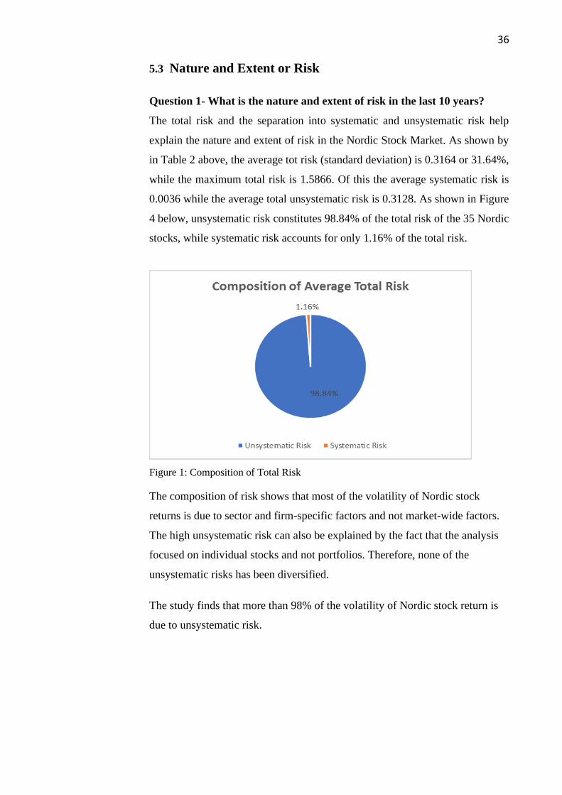
5.3 Nature and Extent or Risk

Question 1- What is the nature and extent of risk in the last 10 years?

The total risk and the separation into systematic and unsystematic risk help

explain the nature and extent of risk in the Nordic Stock Market. As shown by

in Table 2 above, the average tot risk (standard deviation) is 0.3164 or 31.64%,

while the maximum total risk is 1.5866. Of this the average systematic risk is

0.0036 while the average total unsystematic risk is 0.3128. As shown in Figure

4 below, unsystematic risk constitutes 98.84% of the total risk of the 35 Nordic

stocks, while systematic risk accounts for only 1.16% of the total risk.

Figure 1: Composition of Total Risk

The composition of risk shows that most of the volatility of Nordic stock

returns is due to sector and firm-specific factors and not market-wide factors.

The high unsystematic risk can also be explained by the fact that the analysis

focused on individual stocks and not portfolios. Therefore, none of the

unsystematic risks has been diversified.

The study finds that more than 98% of the volatility of Nordic stock return is

due to unsystematic risk.

37

5.4 Jensen Alpha

Question 2- Has the Nordic stock market underperformed or outperformed

the expected return (CAPM) in the last 10 years?

This section answers the second research question. The actual return on the

stocks is compared with the CAPM required returns to assess whether they

have outperformed the market or not. The analysis shows that out of the 35

stocks, only two had negative Jensen alpha. 33 other stocks had positive

Jensen Alpha, implying that their actual returns exceeded the CAPM required

returns. The average Jensen Alpha is 16.22%, showing that on average, the

Nordic stocks outperformed the market by 16.22%. The maximum Jensen

alpha is 89%, indicating that the best performing stock delivered almost twice

the CAPM required return.

The analysis shows that the Nordic Stock market has outperformed the market

(expected return) in the last ten years between 2009 and 2019.

5.5 Findings of t-tests

Question 3- Is there any change in systematic, unsystematic and total risks

in Nordic stock market in the last 10 years between 2009 and 2019?

This section compares the stocks’ systematic and unsystematic risk between

2009 and 2019.

Table 3.2: t-test outputs

As shown in Table 3.2 above, the t-stat for the difference in systematic risk

between 2009 and 2019 is -10.125. The corresponding p-value is 0.000. The

2008/2009 2018/2019 2008/2009 2018/2019

Mean -0.000446419 0.00291486 Mean 0.023007689 0.01337127

Variance 1.66864E-06 1.80786E-06 Variance 4.55289E-05 1.13271E-05

Observations 35 35 Observations 35 35

Pearson Correlation -0.109547317 Pearson Correlation 0.280533334

Hypothesized Mean Difference 0 Hypothesized Mean Difference 0

df 34 df 34

t Stat -10.12539806 t Stat 8.583388882

P(T<=t) one-tail 4.23504E-12 P(T<=t) one-tail 2.50141E-10

t Critical one-tail 1.690924255 t Critical one-tail 1.690924255

P(T<=t) two-tail 8.47008E-12 P(T<=t) two-tail 5.00282E-10

t Critical two-tail 2.032244509 t Critical two-tail 2.032244509

UnSystematic RiskSystematic Risk

38

value is less than 5% implying that there is adequate proof to refute the null

hypothesis (Lind, et al., 2019). Therefore, it can be concluded that there has

been a significant change in systematic risk of Nordic stocks between 2009

and 2019 (Lind, et al., 2019). A comparison of the two means suggests that

systematic risk of the Nordic stocks has increased in the last ten years.

The p-value of the test of difference of unsystematic risk is 0.000. This

indicates that there is a significant difference between the mean of

unsystematic risk in 2009 and 2019. It implies that there has been a significant

change in unsystematic risk of Nordic stocks in the last years (Lind, et al.,

2019). The two means suggest that unsystematic risk has decreased in the

Nordic stock market.

5.6 Cross-Sectional Regression: Relationship between Risk and

Return

Question 4- What is the relationship between risk and return of stocks

listed on the Nordic Stock market?

5.6.1 Expected Return and Beta

The first cross-sectional regression model shows the association between

expected returns and beta. The model’s output is shown in Table 5.3 below.

Table 3.3: Regression model of returns and beta

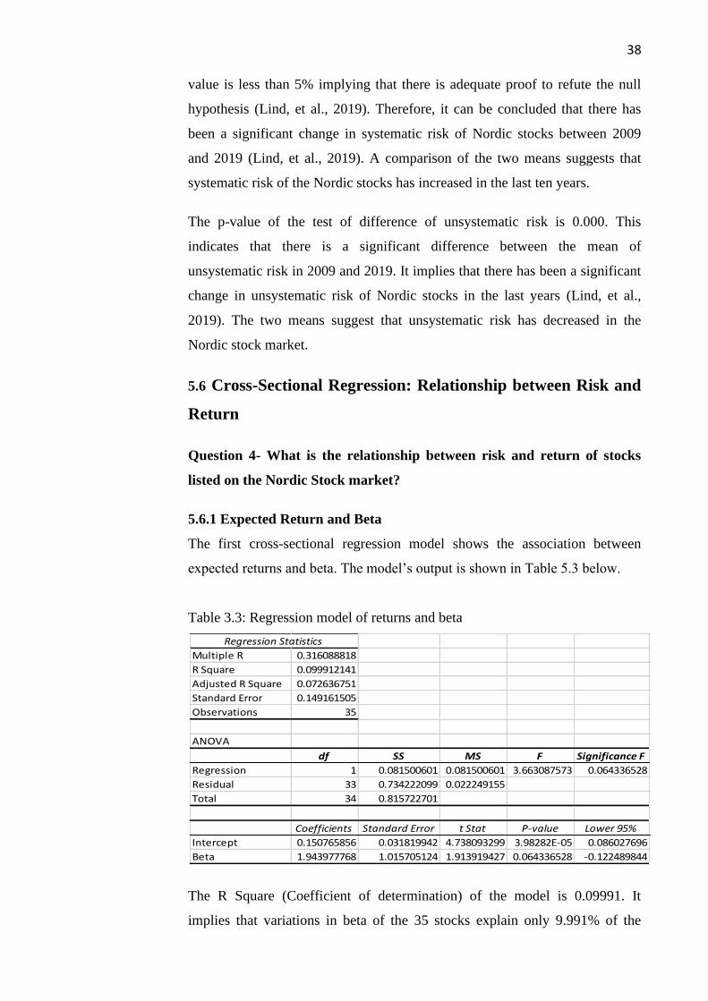
The R Square (Coefficient of determination) of the model is 0.09991. It

implies that variations in beta of the 35 stocks explain only 9.991% of the

Regression Statistics

Multiple R 0.316088818

R Square 0.099912141

Adjusted R Square 0.072636751

Standard Error 0.149161505

Observations 35

ANOVA

df SS MS F Significance F

Regression 1 0.081500601 0.081500601 3.663087573 0.064336528

Residual 33 0.734222099 0.022249155

Total 34 0.815722701

Coefficients Standard Error t Stat P-value Lower 95%

Intercept 0.150765856 0.031819942 4.738093299 3.98282E-05 0.086027696

Beta 1.943977768 1.015705124 1.913919427 0.064336528 -0.122489844

39

variations in actual returns on the stocks between 2009 and 2019 (Pardoe

2012). It suggests that beta explain a small percentage of the variations in

stock returns. More than 90% of the variations in stock returns is explained by

variables other than systematic risk. The model’s coefficient of determination

is small implying that its predictive power is low (Pardoe 2012). This indicates

that the model is not a good predictor of actual daily returns on stocks trading

on the Nordic Stock Market.

To determine if beta was the only determinant of the actual daily stock returns

of the 35 companies listed on the Nordic Stock Exchange, the intercept of the

model was tested for significance. The intercept of the model is 0.1508

suggesting that the average return on a stock would be 15.08% if beta is zero,

that is if systematic risk is zero (Pardoe 2012). The significance of the

intercept is determined by testing the null hypothesis that it is zero or

significantly close to zero. The t-statistic of the intercept is 4.738 with a p-

value of 0.0000398. The p-value is less than 5%, indicating that there is

sufficient proof to reject the null hypothesis. This implies that the claim that

the intercept of the model is zero or significantly close to zero is false.

Therefore, it can be concluded that the intercept of this model is not equal to

zero. The implication of the results is that the intercept is statistically

significant, meaning that beta is not the only determinant of actual returns on

stocks listed on the Nordic Stock Market (ibid.)

The coefficient of beta in the above model is 1.944 suggesting a positive

association between beta and actual daily returns on stocks listed on the Nordic

Stock Market (Graham 2011). It implies that a unit increase in beta (systematic

risk) is associated with an increase in the actual return by 1.944. This appears

consistent with the CAPM, which argues that higher systematic risk attracts a

higher return since investors require a high return to compensate for the high

risk. The t-statistic of the coefficient of beta is 1.914, and the corresponding p-

value is 0.0643. The p-value is higher than 0.05 implying that there is

inadequate evidence to reject the null hypothesis that the coefficient is zero

(Graham 2011). This means that the slope of beta is not statistically

significant. That is, beta has no significant association with actual stock

returns.

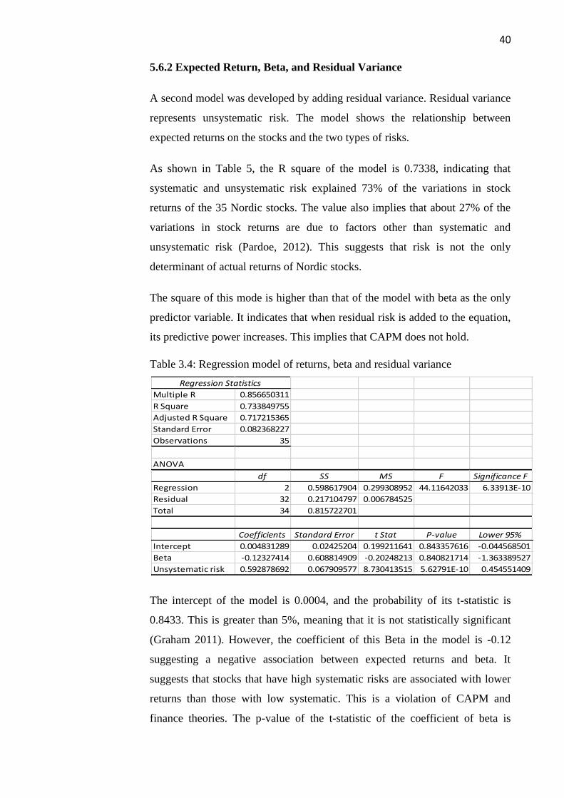
40

5.6.2 Expected Return, Beta, and Residual Variance

A second model was developed by adding residual variance. Residual variance

represents unsystematic risk. The model shows the relationship between

expected returns on the stocks and the two types of risks.

As shown in Table 5, the R square of the model is 0.7338, indicating that

systematic and unsystematic risk explained 73% of the variations in stock

returns of the 35 Nordic stocks. The value also implies that about 27% of the

variations in stock returns are due to factors other than systematic and

unsystematic risk (Pardoe, 2012). This suggests that risk is not the only

determinant of actual returns of Nordic stocks.

The square of this mode is higher than that of the model with beta as the only

predictor variable. It indicates that when residual risk is added to the equation,

its predictive power increases. This implies that CAPM does not hold.

Table 3.4: Regression model of returns, beta and residual variance

The intercept of the model is 0.0004, and the probability of its t-statistic is

0.8433. This is greater than 5%, meaning that it is not statistically significant

(Graham 2011). However, the coefficient of this Beta in the model is -0.12

suggesting a negative association between expected returns and beta. It

suggests that stocks that have high systematic risks are associated with lower

returns than those with low systematic. This is a violation of CAPM and

finance theories. The p-value of the t-statistic of the coefficient of beta is

Regression Statistics

Multiple R 0.856650311

R Square 0.733849755

Adjusted R Square 0.717215365

Standard Error 0.082368227

Observations 35

ANOVA

df SS MS F Significance F

Regression 2 0.598617904 0.299308952 44.11642033 6.33913E-10

Residual 32 0.217104797 0.006784525

Total 34 0.815722701

Coefficients Standard Error t Stat P-value Lower 95%

Intercept 0.004831289 0.02425204 0.199211641 0.843357616 -0.044568501

Beta -0.12327414 0.608814909 -0.20248213 0.840821714 -1.363389527

Unsystematic risk 0.592878692 0.067909577 8.730413515 5.62791E-10 0.454551409

41

0.8408. This is greater than 0.05, indicating that beta has no significant impact

on actual returns (Graham 2011). On the other hand, the p-value of the t-

statistic of the slope of unsystematic risk is 0.000, implying that it is

statistically significant. Therefore, only unsystematic risk (residual risk) has a

significant impact on actual returns.

Therefore, from the above analysis, two conclusions can be seen. First, the

intercept is statistically significant implying that there are other significant

influencers of actual stock returns other than the stocks’ systematic risk (beta).

Secondly, the coefficient of beta is not statistically significant suggesting that

beta did not have a significant association with actual returns of the 35 stocks

listed on the Nordic Stock Market between 2009 and 2019. The results are a

violation of the CAPM which asserts that the return on an asset is dependent

on its systematic risk (beta). Thus, the CAPM was not valid for stocks listed on

the Nordic Stock Market between 2009 and 2014. The findings of this study

imply that CAPM is not accurate and should not be used in estimating the

required returns of Nordic stocks. The results are consistent with the findings

of Miller, et al. (1972), Levy (1978) and Östermark (1991), who found that

beta is not a good predictor of stock returns. Miller, et al. (1972) found that

beta explained only 21% of the variations in stock returns, and that is not

statistically significant. When residual variance was added to the model, the R

squared increased (Miller, et al. 1972). In this analysis, the addition of residual

variance increased the model’s R square from 9% to 73%.

5.7 Chapter Summary

This chapter presents the results of data analysis to assess the relationship

between returns and risk, and to test the validity of CAPM in the Nordic stock

market. The first objective was to determine the nature and extent of risk.

Returns and standard deviations were calculated, and time-series regression

used to estimate beta for each stock was estimated. Analysis of risks indicates

that 98% of the total volatility of stock returns was accounted for by

unsystematic risk, with systematic risk accounting for less than 1.5% of the

volatility of stock returns. Jensen Alpha indicated that the 35 stocks

outperformed the market (required returns). Only two of the 35 stocks had

negative Jensen Alpha. T-tests for the differences in systematic and

42

unsystematic risk between 2009 and 2019 rejected the respective null

hypotheses, implying that there was a significant change in both systematic

and unsystematic risk in the last ten years.

The validity of the CAPM was tested using two cross-sectional regression

models as applied by Miller et al. (1972) and Levy (1978). The first model

showed that there is no significant association between beta and actual returns.

The model’s R square indicated that beta explained only 9% of the variations

in actual returns of Nordic stocks. Significance tests of the model further

suggested that the intercept was statistically significant, implying that beta is

not the only determinant of returns. Besides, beta is not statistically significant

suggesting that systematic risk has no significant impact on Nordic stock

returns. When residual variance was added, the model’s R square increased to

73%, thereby rejecting the claim that only beta determines stock returns. Beta

was not statistically significant in the second model, while residual variance

(unsystematic risk) was statistically significant. These findings provide

evidence against the validity of CAPM in the Nordic stock market. The results

were consistent with previous empirical studies by Miller et al. (1972) and

Levy (1978) who used the same methodology and concluded that CAPM is not

valid.

6. CONCLUSION AND RECOMMENDATION

6.1 Conclusions

The study has focused on CAPM and its significance in estimating the returns

of investments. The study aim was to determine the performance of the Nordic

stock market over a ten-year period between 2009 and 2019. The study had

two main questions, which were set as follows: Is there any change in

systematic risk in between 10 years in Nordic stock market?And does the

Nordic stock market underperformed or over performed in 10 years? The

concept of CAPM has been seen to have originated in the mid-20th century,

after which interest continued to grow over the decades. As the concept grew

more popular, it attracted the interest of scholars and other researchers, and in

time, several studies were made which tested the underpinning theory of the

model as well as evaluated its effectiveness in predicting performance.

Theoretical concepts associated with CAPM include return and rate of return,

43

risk (both systematic and unsystematic), diversification of investment

portfolios and beta, which affects the market as a whole.The study combined

these concepts in the formula

Ra= Rrf + [β * (Re – Rrf)] where,

”Ra” denotes expected return on the security,

”Rrf” denotes risk free rate,

”β” denotes beta,

”Re” denotes expected return of market,

(Re – Rrf) denotes risk premium

Using this formula, the study relied on secondary data gathered from the

Nasdaq Nordic andsampled 35 companies. From the study, it was found that

CAPM is not useful in predicting the performance of Nasdaq Nordic. The

study also found that the findings are consistent with the previous findings

which also reached the conclusion that CAPM is not useful in predicting

performance of stocks in a market.

6.2 Summary and Discussion

From the descriptive statistics, it was found that the average beta was 0.0191,

while the maximum beta was 0.759. What this implies is that the selected

Nordic stocks had a systematic risk of 99% lowerthan the index.Further, the

Jensen Alpha analysis showed that the Nordic stock has outperformed the

market’s expected return based on CAPM productions. Looking at the t-test

values, there has been a significant change in the systematic risk in Nordic

stocks, and at the same time, there has been a significant change in the

unsystematic risk of this market. These findings are in line with the findings of

various previous studies, including those of Pardoe (2012) and Lind et al.

(2019) both of whom also reached similar conclusions.

CAPM is one of the most commonly used models in estimating returns on

investment. The model is applied in calculating the cost of capital, which is

critical in evaluating and appraising long-term investment decisions such as

the acquisition of fixed assets, expansion, among other capital budgeting

decisions. CAPM assumes that investors base their investment decisions on

44

risk and return. It shows the relationship between risk and return. The model

assumes that investors can establish efficient portfolios and diversify all

unsystematic risk. Therefore, only systematic risk should be considered in

estimating returns. Since the fundamental premises of CAPM is the risk-return

relationship, it is essential to understand the relationship between risk and

return to make sound investment decisions. This study analyzed data of 35

stocks listed on the Nordic stock markets to determine the nature and extent of

risk, and to tests whether both systematic and unsystematic risks have changed

over the last ten years. It also tested the validity of CAPM using cross-

sectional regression. Analysis of data suggests that unsystematic risk

constitutes about 98% of the total volatility of returns on Nordic stock markets.

Jensen alpha was used to compare actual performance to the required returns,

and found that the Nordic stocks outperformed the market or their required

returns. Tests of difference in samples indicated that there was a significant

change in both systematic and unsystematic risk of Nordic stocks between

2009 and 2019.

Cross-sectional regression was used to determine the association between risk

and return. In the model between returns and beta, it was found that beta is not

statistically significant and explained only 9% of the variations of actual

returns on the stocks. When residual variance was added to the model, the R

square increased to 73%. Only residual variance was found to be statistically,

with beta not having a significant effect on returns. The data seem to reject the

validity of CAPM in the Nordic stock market. The findings were similar to

those of Miller et al. (1972) and Levy (1978) who concluded that CAPM is not

valid.

The implication of the findings is that investors in the Nordic stock markets

should not rely on CAPM for estimating returns, especially when dealing with

individual stocks. CAPM is not valid and not reliable for estimating returns as

the study provides evidence against the validity of its assumptions.

45

6.3 Limitations of the Study

The study analyzed betas and returns of stocks and not portfolios. The CAPM

assumes that investors can eliminate all unsystematic risk by diversifying their

portfolios. The study used individual stocks, implying that no unsystematic

risk was diversified. With only 35 stocks, it was not possible to create

adequate sample of portfolios to test CAPM. This may have affected the

relationship between risk and return. According to Roll (1977), CAPM

presupposes that the index used in determining beta is efficient. In this study, it

was assumed that the OMX Nordic 40 Index is efficient. This is not realistic

since there can never be perfectly efficient markets in real life. Roll (1977)

further argue that CAPM is forward-looking since it determines expected

returns. Therefore, the use of historical data in testing CAPM can be

misleading.

6.4 Recommendations for Future Research

Based on the study, three recommendations are given. First, it is recommended

that investors in the Nordic stock markets should not rely on CAPM for

estimating returns, especially when dealing with individual stocks. The reason

is that CAPM is not valid and not reliable for estimating returns. The findings

of this study have shown that CAPM is not a valid measure for investors

because the beta did not have a significant association with actual returns of

the 35 stocks listed on the Nordic Stock Market between 2009 and 2019.

Further, any links between CAPM and returns were found to be insignificant,

and this is consistent with the previous findings in some of the studies cited in

the literature.

Secondly, it is also recommended that the managers should consider other

alternative models that predict the performance of organisations other than the

systematic and beta proposed in CAPM. One suggestion is using Multi Beta

Models. Unlike CAPM, which uses a single beta, multi-beta models use

various market risks, thus having more than one beta to predict risk. The

proposed models are the Arbitrage Pricing Model and The Multifactor model.

Thirdly, this study had a number of limitations, the main one being that it

focused primarily on the Nordic stock market but used a small sample size.

46

Thus, it is recommended that future studies look at a larger dataset within this

market to offer a supporting study that can confirm or contrast these findings.

Further, future studies on CAPM should develop efficient portfolios to test the

validity of CAPM. This will, ensure that all unsystematic risk is diversified

thus giving accurate estimates of beta. Besides, studies should focus on

identifying efficient portfolios for proxies as the market return. As outlined by

Roll (1977), if the benchmark is not efficient then the estimates of beta would

not be accurate.

47

7. REFERENCES

ACCA. 2019. CAPM: Theory, advantages and disadvantages. Accessed on

20 october 2019. Retrieved from

https://www.accaglobal.com/in/en/student/exam-support-

resources/fundamentals-exams-study-resources/f9/technical-

articles/CAPM-theory.html

Andrew,Lo. 2008. Finance theory. Accessed on 29 october 2019. Retrieved

from https://ocw.mit.edu/courses/sloan-school-of-management/15-401-

finance-theory-i-fall-2008/

Anwar, M., & Kumar, S. (2018). CAPM - Empirical Evidence from the

Indian Stock Market. Accessed on 1 novemvber 2019. Retrieved from doi:

10.17010/ijrcm/2018/v5/i4/141546

Brooks, R., and Upton, K. 2017. Bond Portfolio Holding PeriodReturn

Decomposition. Journal of Investing, pp.77-90

Brealey, A., Myers, S., and Allen, S. 2011. Principles of corporate finance.

10th edition

Bodie, Z., Kane, A., and Marcus, A. 2004. Essentials of investments.5th

edition New York

Baker,H. And Filbeck, G. (2013). Portfolio theory and management. New

York

Black, F., Jensen, M., and Scholes, M. (1972). The Capital Asset Pricing

Model

Brigham, E. And Houston, J. (2016). Fundamentals of financial

management. Boston.

48

Boďa, M. And Kanderová, M. (2014). Linearity of the Sharpe-lintner

Version of the Capital Asset Pricing Model. Procedi. Pg. 1136-1147.

Brown,P and Walter, T. 2012. The CAPM: Theoretical Validity, Empirical

Intractability and Practical Applications. Pg. 44-50.

Clayman, M. Fridson and Troughton, G. 2012. Corporate Finance: A

Practical Approach.

CFI. 2019. What is the required rate of return. Accessed on 21 october

2019. Retrieved from

https://corporatefinanceinstitute.com/resources/knowledge/trading-

investing/risk-and-return/

Creswell. 2014. CAPM. Accessed on 26 october 2019. Retrieved from

https://gul.gu.se/public/pp/public_file_archive/archive.html?publishedItem

Id=42564721&courseId=86421&fileId=42564716

CFI. 2019. What is CAPM? Accessed on 11 november 2019. Retrieved

from

https://corporatefinanceinstitute.com/resources/knowledge/finance/what-is-

capm-formula/

CFI. 2019. What is Mean- Variance Analysis? Accessed on 30 october

2019. Retrieved from

https://corporatefinanceinstitute.com/resources/knowledge/trading-

investing/mean-variance-analysis/

Dempsey, M. 2013. The Capital Asset Pricing Model : The History of a

Failed Revolutionary Idea in Finance.

Drobny, S. 2010. The invisible hands. New Jersey: John Wiley and Sons,

Inc

49

Fabozzi, F. Rachev, S. Focardi, S and Hoechstoetter, M. 2013. Probability

and statistics for finance

Fama, E and French, K. 2003. The Capital Asset Pricing Model: Theory

and Evidence. Journal of Economic Perspectives pg. 25-46

Fama, E and MacBeth, J. 1973. Risk, Return and Equilibrium. Pg. 607.

Götz and Norbert. 2003. "Norden: Structures That Do Not Make a

Region". Pg. 323–341.

Gitman, L and Zutter, C. 2015. Principles of managerial finance.

Gitman, L. Joehnk, M and Smart, S. 2015. Fundamentals of investing.

Boston.

Graham, A. 2011. Statistics. London.

Guerard, J and Schwartz, E. 2010. Quantitative corporate finance. New

York.

Hotvedt, E. and Tedder. 1978. Systematic and unsystematic risk of rates of

return. Accessed on 28 october 2019. Retrieved from

ageconsearch.umn.edu/bitstream/30276/1/10010135.pdf

Ilmanen, A. 2012. Expected Returns an Investor's . United Kingdom.

Karp, A and Van Vuuren, G. 2017. The Capital Asset Pricing Model And

Fama-French Three Factor. Pg. 231-256.

John,B. 2014. "Nasdaq drops OMX name from branding". Nasdaq Nordic

(2019) Annual trading statistics. Accessed on 11 november 2019.

Retrieved from

http://www.nasdaqomxnordic.com/digitalAssets/110/110020_annual-

statistics-nordic-2018.pdf

50

John, G. 2019. What are difference among required, expected and realized

rate of return?. Accessed on 25 october 2019. Retrieved from

https://www.brighthub.com/money/personal-finance/articles/16790.aspx

Lind, D., Marchal, W and Wathen, S. 2019. Basic statistics for business

and economics. New York.

Linden,A., Trochim,W. and Adams,J. 2006. Evaluating Program

Effectiveness Using the Regression Point. pg.406-424.

Markowitz, H. 2016. Risk-Return Analysis. New York.

Michelle,R. 2018. What is rate of return and what is a good rate of return.

Accessed on 23 october 2018. Retrieved from

https://www.thestreet.com/personal-finance/education/what-is-rate-of-

return-14779699

Mokkelbost,P. 1971. Unsystematic Risk over Time. Pg.785.

Mayo, H. 2012. Basic finance.

McBurney, D and White, T. 2013. Research methods. CA.

Moyer, C. 2005. Contemporary financial management. Ohio.

Novak, J and Petr, D. 2004. CAPM Beta, Size, Book-to-Market, and

Momentum in Realized Stock Returns. Pg. 447-460.

OSC. 2019. The risk and return relationship. Accessed on 21 october 2019.

Retrieved from https://www.getsmarteraboutmoney.ca/invest/investing-

basics/understanding-risk/the-risk-return-relationship/

Östermark, R. 1991. Empirical evidence CAPM in two Scandinavian stock

exchanges market. Pg. 223-234.

Peterson, S. 2012. Investment theory and risk management.

51

Renne, B. Why does low beta mean for a business?. Accessed on 22

october 2018. Retrieved from https://smallbusiness.chron.com/low-beta-

mean-business-26280.html

Research Support. 2019. Research methodology. Accessed on 27 october

2019. Retrieved from

https://libguides.wits.ac.za/c.php?g=693518&p=4914913

Roll, R. 1977. A critique of the asset pricing theory's tests . pg. 129-176.

Satrio, A. 2015. CAPM and Three Factor Model

Saunders, M., Lewis, P., and Thornhill, A. 2009. Research Methods for

Business Students. 5th edition. Harlow

Sandip, R. 2018. Whai is the Jensen’s Alpha? Accessed on 29 october

2019, Retrieved from https://www.plindia.com/blog/what-is-the-jensens-

alpha/

Sibilkov,V. 2007. Asset Liquidity and Capital Structure. Volume 44, pg.

1173-1197

Sreenu, N. 2018. An Empirical Test of Capital Asset-pricing Model and

Three-factor Model of Fama in Indian Stock Exchange. pp. 293-308

Trochim, W. 2005. Research Methods: The Concise Knowledge Base.

Ohio.

Watson,D and Head, A. 2016. Corporate Finance: Principles and Practice.

New York.

Wilson, J. (2019). Essentials of Business Research. Milton: Routledge.

52

Yang, M. 2014. The Risk Return Relationship.SSRN Electronic Journal

Book

Zhao,L. 2015. Credit Risk 'Beta'. Accessed on 27 october 2019. Retreived

from: http://dx.doi.org/10.2139/ssrn.2667055

53

Appendix

Appendix 1. Information of Swedish companies

Serial

Number.

Name of

companies

Industry Website

1 ABB LTD Industrial http://www.abb.com

2 Alfa Laval Industrial http://www.alfalaval.com

3 Assa Abloy B Industrial https://www.assaabloy.com

4 Atlas Copco A Industrial http://www.atlascopcogroup.com

5 Astrazeneca Healthcare http://www.astrazeneca.com

6 Boliden Basic materials http://www.boliden.com

7 Electrolux B Technology https://www.electroluxgroup.com

8 Ericsson B Technology http://www.ericsson.com

9 Hexagon B Technology http://www.hexagon.com

54

10 Hennes &

Mauritz B

Consumer

Cyclical

http://www.hm.com

11 Investor B Financial

services

http://www.investorab.com

12 Nordea Bank

ABP

Financial

services

http://www.nordea.com

13 Sandvik Industrial http://www.sandvik.com

14 SEB A Financial

services

http://www.seb.se

15 SV.

Handelsbanken

A

Financial

services

http://www.handelsbanken.se

16 SKF B Industrial http://www.skf.com

17 Swedbank A Fiancial

services

55

18 Swedish Match Consumer

Defensive

http://www.swedishmatch.com

19 Tele2 B Communication

services

http://www.tele2.com

20 Telia Company Communication

services

http://www.teliacompany.com

21 Volvo B Industrials http://www.volvogroup.com

56

Appendix 2- Information on Denmark companies

Serial

Number

Name of

companies

Industry Website

1 Carlsberg B Consumer

Defensive

http://www.carlsberggroup.com

2 Danske Bank Financial

services

http://www.danskebank.com

3 DSV Panalpina Industrial http://www.dsv.com

4 Genmab Healthcare http://www.genmab.com

5 Novo Nordisk

B

Healthcare http://www.novonordisk.com

6 Novozymes B Basic materials http://www.novozymes.com

7 Vestas Wind

System

Industrial http://www.vestas.com

8 Coloplast B Healthcare http://www.coloplast.com

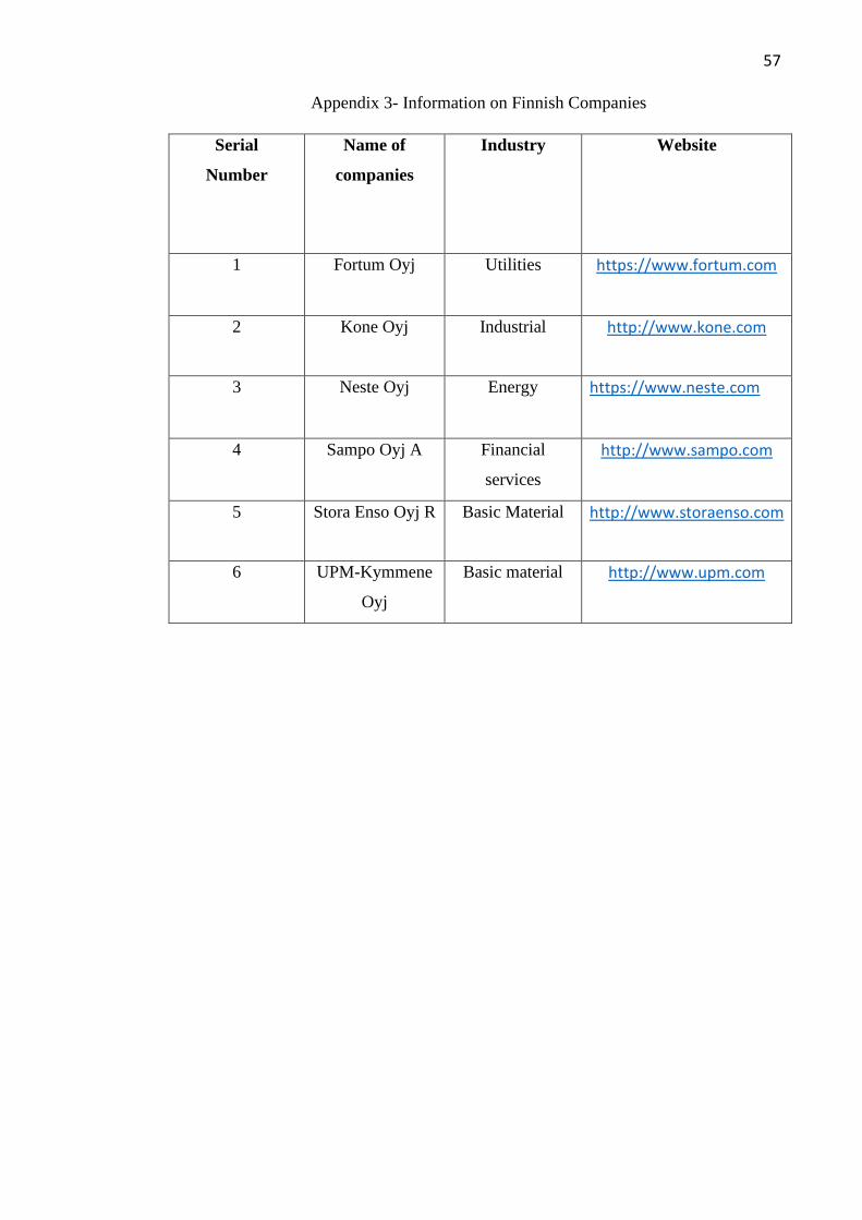
57

Appendix 3- Information on Finnish Companies

Serial

Number

Name of

companies

Industry Website

1 Fortum Oyj Utilities https://www.fortum.com

2 Kone Oyj Industrial http://www.kone.com

3 Neste Oyj Energy https://www.neste.com

4 Sampo Oyj A Financial

services

http://www.sampo.com

5 Stora Enso Oyj R Basic Material http://www.storaenso.com

6 UPM-Kymmene

Oyj

Basic material http://www.upm.com