HAL Id: hal-00747616https://hal.archives-ouvertes.fr/hal-00747616v2

Submitted on 29 Apr 2014

HAL is a multi-disciplinary open accessarchive for the deposit and dissemination of sci-entific research documents, whether they are pub-lished or not. The documents may come fromteaching and research institutions in France orabroad, or from public or private research centers.

L’archive ouverte pluridisciplinaire HAL, estdestinée au dépôt et à la diffusion de documentsscientifiques de niveau recherche, publiés ou non,émanant des établissements d’enseignement et derecherche français ou étrangers, des laboratoirespublics ou privés.

Study of a low Mach nuclear core model for two-phaseflows with phase transition I: stiffened gas law

Manuel Bernard, Stéphane Dellacherie, Gloria Faccanoni, Bérénice Grec,Yohan Penel

To cite this version:Manuel Bernard, Stéphane Dellacherie, Gloria Faccanoni, Bérénice Grec, Yohan Penel. Study ofa low Mach nuclear core model for two-phase flows with phase transition I: stiffened gas law.ESAIM: Mathematical Modelling and Numerical Analysis, EDP Sciences, 2014, 48, pp.1639-1679.�10.1051/m2an/2014015�. �hal-00747616v2�

Study of a low Mach nuclear core model

for two-phase �ows with phase

transition I: sti�ened gas law

Manuel Bernard∗, Stéphane Dellacherie†,

Gloria Faccanoni‡, Bérénice Grec§ and Yohan Penel¶

April 15, 2014

In this paper, we are interested in modelling the �ow of the coolant (water) in anuclear reactor core. To this end, we use a monodimensional low Mach number modelcoupled to the sti�ened gas law. We take into account potential phase transitions bya single equation of state which describes both pure and mixture phases. In someparticular cases, we give analytical steady and/or unsteady solutions which providequalitative information about the �ow. In the second part of the paper, we introducetwo variants of a numerical scheme based on the method of characteristics to simulatethis model. We study and verify numerically the properties of these schemes. We�nally present numerical simulations of a loss of �ow accident (LOFA) induced by acoolant pump trip event.

AMS Classi�cations 35Q35, 35Q79, 65M25, 76T10.

Introduction

Several physical phenomena have to be taken into account when modelling a water nuclearreactor such as PWRs1 or BWRs2 (see [12] for an introduction). In particular, the present workdeals with the handling of high thermal dilation of the coolant �uid induced by thermal transfersin nuclear cores (see Figure 1 for schematic pictures of PWR and BWR reactors). A naturalapproach is to represent the evolution of the �ow by means of a system of PDEs similar to the

∗IFPEN � Lyon, BP 3, 69360 Solaize, France � manuel.bernard@ifpen.fr†DEN/DANS/DM2S/STMF, Commissariat à l'Énergie Atomique et aux Énergies Alternatives � Saclay, 91191Gif-sur-Yvette, France � stephane.dellacherie@cea.fr

‡Université de Toulon � IMATH, EA 2134, avenue de l'Université, 83957 La Garde, France � faccanon@univ-tln.fr§MAP5 UMR CNRS 8145 - Université Paris Descartes - Sorbonne Paris Cité, 45 rue des Saints Pères, 75270Paris Cedex 6, France � berenice.grec@parisdescartes.fr

¶CETMEF-INRIA � team ANGE and LJLL UMR CNRS 7598, 4 place Jussieu, 75005 Paris, France �yohan.penel@cerema.fr

1PWR is the acronym for Pressurized Water Reactor.2BWR is the acronym for Boiling Water Reactor.

1

compressible Navier-Stokes equations coupled to the modelling of phase transition as it is thecase in classic industrial codes [1, 7, 24].

In nominal and incidental situations as well as in some accidental situations studied in safetyevaluations, the magnitude of the sound velocity is much higher than the one of the velocity ofthe coolant �uid, which means that the Mach number of the �ow is small. The discretizationof compressible Navier-Stokes type systems at low Mach number may induce numerical issuesdirectly related to the existence of fast acoustic waves (see for example [15, 28, 42] when theconvective part of the compressible Navier-Stokes system is discretized by means of a Godunovtype scheme). Sereval numerical techniques based on the resolution of a Poisson equation havebeen proposed in the literature to extend incompressible methods to the (compressible) low Machcase. A pioneering work was that of Casulli & Greenspan [9] where a �nite-di�erence scheme overa staggered grid is designed by impliciting terms involving the speed of sound in order to avoidrestrictive stability conditions. In [11], Colella & Pao made use of the Hodge decomposition tosingle out the incompressible part of the velocity �eld.

Nevertheless, in a low Mach number regime, the acoustic phenomena can be neglected in energybalances although the �ow is highly compressible because of the thermal dilation. Thus, toovercome the numerical di�culties, S. Dellacherie proposed in [16] another model obtained by�ltering out the acoustic waves in the compressible model. Let us underline that this approachwas �rst applied to model low Mach combustion phenomena [34,35,41], then astrophysical issues[4, 5] and thermal dilation of the interface of bubbles at low Mach number [13]. This speci�ckind of models have been studied from a theoretical point of view. We mention for instance [21]for the well-posedness of a low Mach number system and [26, 34, 39, 41] for the derivation ofmonodimensional explicit solutions.

From a numerical point of view, 2D simulations have been performed in [4, 5, 30] for astrophys-ical and combustion applications while a numerical study of the model established in [13] wasproposed in [14]. As for the low Mach number model derived in [16] and called the Low MachNuclear Core (Lmnc) model, it was discretized in [6] in the monodimensional (1D) case. More-over, 1D unsteady analytical solutions were also given in [6] which allowed to assess the numericalschemes. Notice that 2D numerical results will be presented in [17,18].

Despite relevant numerical results, the approach proposed in [6, 16] was not satisfying since itwas restricted to monophasic �ows. Thus, we extend in this study the results stated in [6,16] bytaking into account phase transition in the Lmnc model. If we neglect viscous e�ects, the Lmncmodel proposed in this paper may be seen as the low Mach number limit of the HomogeneousEquilibrium Model (HEM) [10,25,29,37,43] with source terms. Let us recall that the HEM modelis the compressible Euler system in which the two phases are supposed to be at local kinematic,mechanic and thermodynamic equilibria.

A crucial step in the process is the modelling of �uid properties through the equation of state(EOS). It is important from a physical point of view to match experimental data and from amathematical point of view to close the system of PDEs. In the present work, this point isachieved by using the sti�ened gas EOS. A major result in this paper is the exhibition of 1Dunsteady analytical solutions with phase transition (see Proposition 3.4). These solutions areof great importance: on the one hand they provide accurate estimates of heat transfers in anuclear core in incidental and accidental situations, and on the other hand they enable to assessthe robustness of the monodimensional numerical schemes presented in this article. In addition,regardless of the EOS used in the pure phases, when the thermodynamic pressure is constant(which is the case in the Lmnc model) and when the phase change is modelled by assuming local

2

Containementstructure

Liquid

Vapor

Steamgenerator

(heat change)

Pump

Reactor core(155 bar)

Reactor vesselControlrods

Pressurizer

Water coolant(output temp.: 330 ◦C)

Water coolant(input temp.: 290 ◦C)

(a) Scheme of the primary circuit of a PWR.

Containementstructure

Pump

Controlrods

Reactor vessel &Steam generator

Reactor core(75 bar)

Pressurizer

Water coolant(output temp.: 290 ◦C)

Water coolant(input temp.: 280 ◦C)

Liquid

Vapor

(b) Scheme of the primary circuit of a BWR.

Figure 1: Scheme of nuclear reactors whose coolant is water: the major di�erence between PWRand BWR is the steam void formation in the core of the latter.

mechanic and thermodynamic equilibria, the mixture can always be considered a sti�ened gas(this point will be clari�ed in the sequel): this important remark legitimates the study of theLmnc model together with the sti�ened gas EOS.

Compared to the numerous low Mach number combustion models derived in the literature, theLmnc model di�ers for several reasons. Some of them are due to the underlying �uids: indeed,combustion issues are related to gas modelled by the ideal gas law and involved in misciblemixtures whereas our modelling comprises a more general equation of state and mixtures ofimmiscible �uids. We must also mention that the system of PDEs is set in a bounded domain withnonperiodic boundary conditions whose in�uence upon theoretical and numerical investigationsis noticeable.

At last, we wish to underline that although this study is speci�c to dimension 1 (which is essentialto obtain in particular the unsteady analytical solutions with phase change), it remains usefulfrom an industrial point of view since many safety evaluations use a 1D modelling to describethe �ow in each component of the nuclear reactor and thus within the nuclear core [7, 19].Nevertheless, the extension of this work to dimensions 2 and 3 is a natural and importantperspective [17].

This paper is organized as follows. In Section 1, the Lmnc model is recalled together withboundary/initial conditions and assumptions under which it is valid. We also study the existenceof (more or less) equivalent formulations of the model that can be used depending on the variableswe aim at focusing on. Section 2 is devoted to the modelling of phase transition and to theEOS that is necessary to close the system. In Section 3, we prove some theoretical resultsstated (without proof) in [6] and we extend them to the multiphasic case. Exact and asymptoticsolutions are thus exhibited. Numerical aspects are then investigated in Section 4. More precisely,we present some numerical schemes based on the method of characteristics proposed in [38]. Wethen prove that these schemes preserve the positivity of the density and of the temperaturefor any time step. Finally, these schemes are applied in Section 5 to various situations withoccurrence of phase transition like a simpli�ed scenario for a Loss of Flow Accident (LOFA)induced by a coolant pump trip event.

3

1. The low Mach nuclear core model

The Low Mach Nuclear Core (Lmnc) model introduced in [16] is obtained by �ltering out theacoustic waves in a compressible Navier-Stokes type system. This is achieved through an asymp-totic expansion with respect to the Mach number assumed to be very small in this framework.One of the major consequences is the modi�cation of the nature of the equations: the �lteringout of the acoustic waves � which are solutions of a hyperbolic equation in the compressiblesystem � introduces a new unknown (namely the dynamic pressure) which is solution to an el-liptic equation in the Lmnc model. Another consequence is that we are able to compute explicitmonodimensional unsteady solutions of the Lmnc model with or without phase transition3 (seeSection 3) and to construct 1D robust and accurate numerical schemes4 (see Section 4).

In this section, we recall the Lmnc model and we present equivalent formulations for smoothsolutions. Since we are interested in the 1D case in this paper, we do not extend results to2D/3D. Nevertheless, this can easily be done (provided the boundary conditions are adapted).

1.1. Governing equations

The 1D nonconservative formulation of the Lmnc model [16] is written as∂yv =

β(h, p0)

p0Φ(t, y), (1.1a)

ρ(∂th+ v∂yh) = Φ(t, y), (t, y) ∈ R+ × [0, L] (1.1b)

∂t(ρv) + ∂y(ρv2 + p) = F(v)− ρg, (1.1c)

where v and h denote respectively the velocity and the (internal) enthalpy of the �uid. Pressurep0 is a given constant � see below. The density ρ = ρ(h, p0) is related to the enthalpy by anequation of state (EOS) � see Section 2. So does the dimensionless compressibility coe�cientβ(h, p0) which is de�ned by

β(h, p0) def=− p0

ρ2(h, p0)· ∂ρ∂h

(h, p0). (1.2)

The power density Φ(t, y) is a given function of time and space modelling the heating of thecoolant �uid due to the �ssion reactions in the nuclear core. Finally, g is the gravity �eld andF(v) models viscous e�ects: the classic internal friction in the �uid, and also the friction on the�uid due to technological devices in the nuclear core (e.g. the friction on the �uid due to thefuel rods). In the sequel, we take

F(v) = ∂y(µ∂yv).

In this case, µ is a turbulent viscosity given by an homogenized turbulent model. Nevertheless,we explain in the sequel that the exact choice of F(v) is not important in the 1D case (this is nomore the case in 2D/3D).

We must also emphasize that model (1.1) is characterized by two pressure �elds, which is classicin low Mach number approaches:

3This is not the case for the 1D compressible system from which the Lmnc is derived.4The existence of fast acoustic waves in the compressible system induces numerical di�culties � see [15, 28] forexample � which cannot arise in the Lmnc model since the acoustic waves have been �ltered out to obtainthis low Mach number model.

4

� p0: this �eld is involved in the equation of state and is named the thermodynamic pressure.It is assumed to be constant throughout the present study and corresponds to an averagepressure in the nuclear core;

� p(t, y): it appears in the momentum equation (1.1c) and is referred to as the dynamicpressure. It is similar to the pressure �eld which appears in the incompressible Navier-Stokes system.

Notice that p0 + p(t, y) is a 1st-order approximation of the classic compressible pressure in thenuclear core: the pressure p(t, y) is indeed a perturbation around the average pressure p0 (thisis due to the low Mach number hypothesis [16]). In the 1D case, equation (1.1c) decouples fromthe two other equations and may be considered a post-processing leading to the computation ofp (this is why the expression of F(v) is not essential in 1D). Thus, equation (1.1c) will often beleft apart in the sequel and equations (1.1a)-(1.1b) will often be referred to as the Lmnc modelfor the sake of simplicity.

1.2. Supplements

From now on, we suppose that:

Hypothesis 1.1.

1. Φ(t, y) is nonnegative for all (t, y) ∈ R+ × [0, L].

2. p0 is a positive constant.

The �rst assumption characterizes the fact that we study a nuclear core where the coolant �uidis heated. In the steam generator of a PWR type reactor (see Figure 1a) � which could also bemodelled by means of a Lmnc type model � the �uid of the primary circuit heats the �uid ofthe secondary circuit by exchanging heat through a tube bundle: in that case, we would haveΦ(t, y) ≤ 0 in the primary circuit and Φ(t, y) ≥ 0 in the secondary circuit.

The second assumption corresponds to real physical conditions even if it is not required in thesetting of the equation of state (see Section 2.3).

Boundary conditions (BC) The �uid is injected at the bottom of the core at a given enthalpyhe and at a given �ow rate De. We also impose the dynamic pressure p at the exit of the core(y = L). The inlet BC are {

h(t, 0) = he(t), (1.3a)

(ρv)(t, 0) = De(t), (1.3b)

while the outlet BC isp(t, L) = 0. (1.3c)

The entrance velocity ve(t) to apply at y = 0 is deduced from the relation

ve(t)def=De(t)

ρe(t)where ρe

def= ρ(he, p = p0). (1.4)

The fact that he andDe depend on time enables to model transient regimes induced by accidentalsituations. For example, when De(t) tends to zero, it models a main coolant pump trip event

5

which is a Loss Of Flow Accident (LOFA) as at the beginning of the Fukushima accident in thereactors 1, 2 and 3.

We also assume in the sequel that:

Hypothesis 1.2.

1. De is nonnegative.

2. he is such that ρe is well-de�ned and positive.

The �rst assumption corresponds to a nuclear power plant of PWR or BWR type: the �owis upward5. The second assumption means that the EOS ρ(h, p) is such that ρ(he, p0) can becomputed. Moreover, we also suppose that ρ(he, p0) > 0 from a physical point of view.

We �nally make the following modelling hypothesis:

Hypothesis 1.3. β is nonnegative.

Positivity assumptions about Φ, De, β and ρ in Hypotheses 1.1, 1.2 and 1.3 ensure that thevelocity v(t, y) remains nonnegative at any time and anywhere in the core. Otherwise, the systemcould become ill-posed (see Section 4.2 in [16] where this question is partially addressed).

Well-prepared initial conditions The model is �nally closed by means of the initial conditionh0(y) = h(0, y) satisfying the following hypothesis:

Hypothesis 1.4.

1. We impose the compatibility condition h0(y = 0) = he(t = 0).

2. h0 is such that ρ0 is well-de�ned and positive.

The initial density deduced from the EOS directly satis�es the equality ρ0(y = 0) = ρe(t = 0).Secondly, as system (1.1) consists of steady and unsteady equations, the initial velocity v0 mustsatisfy equation (1.1a) for t = 0, which means

v′0(y) =β(h0(y), p0

)p0

Φ(0, y).

Hence, h0 prescribes the initial velocity v0 through the previous di�erential equation togetherwith the condition v0(y = 0) = ve(t = 0). The initial �ow rate D0 is thus given by

D0(y) = ρ0(y)v0(y).

Such initial data h0 and D0 are said to be well-prepared. This will be implicitly assumed in thesequel.

5 The �ow could be downward when the nuclear reactor is a material testing reactor.

6

1.3. Origin and di�erent formulations of the model

The 1D Lmnc model (1.1) is written in [16] as ∂yv =β(h, p0)

p0Φ(t, y), (1.5a)

ρ(h, p0) · (∂th+ v∂yh) = Φ(t, y). (1.5b)

We recall that in the 1D case, equation (1.1c) is a post-processing of (1.5). It is important tonote that the low Mach number model (1.5) is justi�ed only under smoothness assumptions. Tostudy the existence of weak solutions, it might be better to use a conservative formulation whichis equivalent to (1.5) for smooth solutions. This conservative formulation is the following:

Proposition 1.1. Under smoothness assumptions, system (1.5) is equivalent to{∂tρ+ ∂y(ρv) = 0, (1.6a)

∂t(ρh) + ∂y(ρhv) = Φ(t, y). (1.6b)

System (1.6) (coupled to equation (1.1c)) is the Lmnc model written in conservative variables.Although (1.6) is more general than (1.5), system (1.5) is interesting as it emphasizes the factthat the �ltering out of the acoustic waves turns the hyperbolic nature of the compressibleNavier-Stokes system (related to the acoustic waves) to an elliptic constraint (upon the velocity)similar to the incompressible case.

Moreover, under smoothness assumptions and for a particular class of EOS, we can derive asemi-conservative formulation equivalent to (1.5), and which may be useful to derive e�cientnumerical schemes. Indeed, we have the following proposition.

Proposition 1.2. Under smoothness assumptions:

1. System (1.5) implies ∂yv =β(h, p0)

p0Φ(t, y), (1.7a)

∂t(ρ(h, p0)h

)+ ∂y

(ρ(h, p0)hv

)= Φ(t, y). (1.7b)

2. For equations of state such that

∂ρ

∂h(h, p0) 6= −ρ(h, p0)

h, (1.8)

systems (1.5) and (1.7) are equivalent.

Condition (1.8) upon ρ seems to be quite restrictive insofar as it does not enable to handle idealgas (for which ∂ρ

∂h = − ρh ). In the latter case, equations (1.7a) and (1.7b) are nothing but the

same equation, which implies that we have to use formulations (1.5) or (1.6).

Remark 1.1. The equivalence between systems (1.5), (1.6) and (1.7) also holds in higher di-mensions. Nevertheless, the momentum equation is strongly coupled to the other equations in2D/3D and must be taken into account under conservative or nonconservative forms. Indeed,these forms are equivalent (as soon as the unknowns are smooth).

7

Proof of Proposition 1.1.

• ⇒ According to de�nition (1.2) of β, we have

∂tρ+ ∂y(ρv) =∂ρ

∂h(∂th+ v∂yh)︸ ︷︷ ︸

(1.5b)= Φ

ρ

+ρ ∂yv︸︷︷︸(1.5a)

= βΦp0

= 0 (1.9)

which gives (1.6a). We also obtain

∂t(ρh) + ∂y(ρhv) = h(∂tρ+ ∂y(ρv)

)+ ρ (∂th+ v∂yh) = Φ,

using (1.5b) and (1.6a). We recover (1.6b).

• ⇐ Because of (1.6a), we deduce (1.5b) from (1.6b). Moreover, we deduce from (1.6a) and(1.5b) that

∂tρ+ ∂y(ρv) =∂ρ

∂h(∂th+ v∂yh) + ρ∂yv =

∂ρ

∂h· Φ

ρ+ ρ∂yv = 0,

which gives (1.5a) thanks to de�nition (1.2) of β.

Proof of Proposition 1.2. The �rst point is a direct consequence of Proposition 1.1 since

∂t(ρ(h, p0)h

)+ ∂y

(ρ(h, p0)hv

)= ρ(h, p0) · (∂th+ v∂yh)︸ ︷︷ ︸

(1.5b)= Φ

+h[∂t(ρ(h, p0)

)+ ∂y

(ρ(h, p0)v

)]︸ ︷︷ ︸(1.9)= 0

.

To prove the second point, we just have to show that (1.7) implies (1.5) under condition (1.8).On the one hand, since

∂tρ+ ∂y(ρv) =∂ρ

∂h(h, p0)(∂th+ v∂yh) + ρ(h, p0)∂yv,

by using (1.2) and (1.7a), we obtain

∂tρ+ ∂y(ρv) =∂ρ

∂h(h, p0)

(∂th+ v∂yh−

Φ

ρ(h, p0)

). (1.10)

On the other hand, (1.7b) leads to

ρ(h, p0) · (∂th+ v∂yh) + h[∂t(ρ(h, p0)

)+ ∂y

(ρ(h, p0)v

)]= Φ(t, y)

that is to say

∂tρ+ ∂y(ρv) = −ρ(h, p0)

h

(∂th+ v∂yh−

Φ

ρ(h, p0)

). (1.11)

Thus, by comparing (1.10) and (1.11), we obtain

∂th+ v∂yh−Φ

ρ(h, p0)= 0

under condition (1.8), which proves that (1.7) implies (1.5).

8

2. Equation of state for two-phase �uids

For the system to be closed, an additional equation is required: the equation of state (EOS). Itcorresponds to the modelling of thermodynamic properties and consists of an algebraic relationbetween thermodynamic variables. Indeed, perturbations of the inlet velocity or of the powerdensity may strongly modify the temperature in the �uid and cause phase transition from liquidphase to vapor phase. At this modelling scale, the �uid can thus be under liquid, vapor ormixture phases. The issue is here to construct an EOS that models all phases of a �uid.

The model used in this study is based on the assumption of local mechanic and thermodynamicequilibria between phases. This means that the phases are assumed to move at the same velocityand that vaporisation, condensation and heat transfer processes are assumed to be instantaneous.As a consequence, the two-phase �ow can be considered a single-phase problem provided the EOS(h, p) 7→ ρ(h, p) (and thus the compressibility coe�cient β de�ned by (1.2)) takes phase transitioninto account. With this modelling, the two-phase �ow evolution at low Mach number can bedescribed by means of the Lmnc model (1.1). In this case and when viscous e�ects modelled byF(v) in (1.1c) are neglected, the Lmnc model (1.1) is the low Mach limit of the HomogeneousEquilibrium Model (HEM) [10,25,29,37,43] with source terms.

2.1. General thermodynamics

In classic thermodynamics, two variables are su�cient to represent a thermodynamic state ofa pure single-phase �uid. This is done by means of an EOS which is a relation between theinternal energy, the density and the entropy. In the literature, there exist numerous EOS speci�cto the �uid and to the model which are under consideration. In the case of liquid-vapor phasetransitions, the EOS must not only represent the behavior of each pure phase (liquid or vapor),but also model the rate of the mass transfer between one phase to the other.

Phase diagram of Figure 2b represent the coexistence curve ps(T ) which relates the pressure tothe temperature when phase change occurs: the plane (T, p) is split by the coexistence curveinto two regions in which one phase or another is stable. At any point on such a curve the twophases have equal Gibbs potentials and both phases can coexist.

In the (1/ρ, p) plane (see Figure 2a) this mixture where both phases coexist is called the saturationzone. The designation �at saturation� means that the steam is in equilibrium with the liquidphase. This region is bounded by two curves connected at the critical point (1/ρc, pc) which alsobelongs to the critical isotherm T = Tc. Within the two-phase region, through any point passesan isotherm which is a straight line.

These curves can be obtained experimentally (see [33] for instance) and correspond to thermo-dynamic equilibria of temperature, pressure and Gibbs potential of the two phases. The Van derWaals law associated to the Maxwell construction is the most common example of this kind ofEOS.

Nevertheless, it is very complicated to derive a unique EOS describing accurately both pure andmixture phases. To better handle pure phases and saturation curves, an idea consists in usingtwo laws (one for each phase) so that each phase has its own thermodynamics. In the followingsection, we detail the general construction of the EOS in the mixture region given one EOS foreach phase.

9

iso-T with

T = Tc

saturated

liquid

curve

saturated

vapor

curve

critical

point

C

1ρc

pc

1ρ

p

iso-T with

T < Tc

L Vps(T )

triple line

liquid

liquid-vapor mixture

vapor

1ρs`(T )

1ρsg(T )

(a) Since the phase transition appears at constant pressureand temperature, the physical isotherm is horizontal inthe mixture region and coincide with the isobar. Atcritical point C, the isotherm T = Tc has a horizontaltangent.

T

p

triple

point

critical

point

liquid

vapor

Tc

pc

(b) Coexistence curve ps(T )

Figure 2: Saturation and coexistence curves.

2.2. Construction of the EOS in the mixture

In this section, we explain how to specify the EOS in the mixture given an EOS for each purephase.

Characterization of the two-phase media We consider each phase κ (κ = ` for the liquid phaseand κ = g for the vapor phase) as a compressible �uid governed by a given EOS: (ρ, ε) 7→ ηκ whereρ, ε and ηκ denote respectively the speci�c density, the speci�c internal energy and the speci�centropy of the �uid. We assume that the function (τ, ε) 7→ ηκ(1/τ, ε) has a negative-de�niteHessian matrix where τ def= 1/ρ is the speci�c volume [8].

We then de�ne classically for any phase κ the temperature Tκ, the pressure pκ and the chemicalpotential gκ respectively by

Tκdef=

(∂ηκ∂ε

∣∣∣∣ρ

)−1

, pκdef=−ρ2Tκ

∂ηκ∂ρ

∣∣∣∣ε

, gκdef= ε+

pκρ− Tκηκ.

Finally α denotes the volume fraction of vapor phase. This variable characterizes the volume ofvapor in each unit volume: α = 1 means that this volume is completely �lled by vapor; similarly,a full liquid volume corresponds to α = 0. Liquid and vapor are thus characterized by theirthermodynamic properties.

The mixture density ρ and the mixture internal energy ε are de�ned by{ρ def= αρg + (1− α)ρ`, (2.1a)

ρε def= αρgεg + (1− α)ρ`ε`, (2.1b)

where ρg, ρ`, εg and ε` denote respectively vapor/liquid densities and vapor/liquid internalenergies. Recalling that the internal energy is connected to the enthalpy by the relation ρh =

10

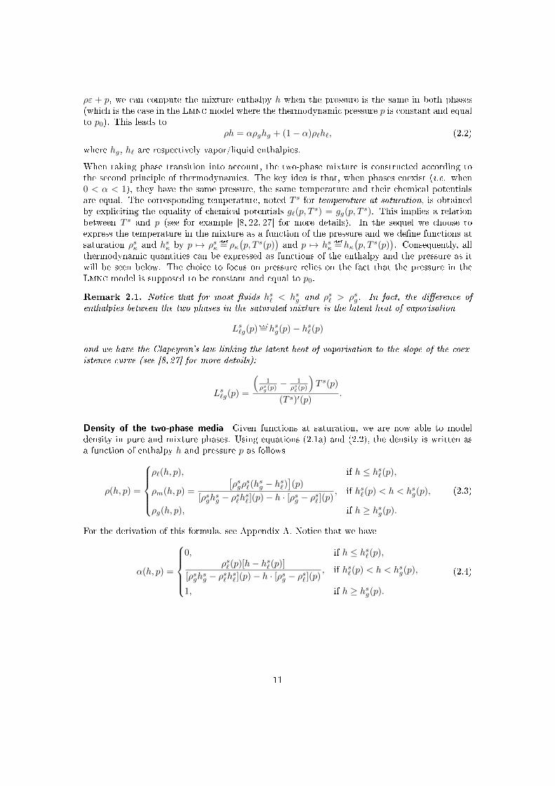
ρε + p, we can compute the mixture enthalpy h when the pressure is the same in both phases(which is the case in the Lmnc model where the thermodynamic pressure p is constant and equalto p0). This leads to

ρh = αρghg + (1− α)ρ`h`, (2.2)

where hg, h` are respectively vapor/liquid enthalpies.

When taking phase transition into account, the two-phase mixture is constructed according tothe second principle of thermodynamics. The key idea is that, when phases coexist (i.e. when0 < α < 1), they have the same pressure, the same temperature and their chemical potentialsare equal. The corresponding temperature, noted T s for temperature at saturation, is obtainedby expliciting the equality of chemical potentials g`(p, T s) = gg(p, T

s). This implies a relationbetween T s and p (see for example [8, 22, 27] for more details). In the sequel we choose toexpress the temperature in the mixture as a function of the pressure and we de�ne functions atsaturation ρsκ and hsκ by p 7→ ρsκ

def= ρκ(p, T s(p)

)and p 7→ hsκ

def= hκ(p, T s(p)

). Consequently, all

thermodynamic quantities can be expressed as functions of the enthalpy and the pressure as itwill be seen below. The choice to focus on pressure relies on the fact that the pressure in theLmnc model is supposed to be constant and equal to p0.

Remark 2.1. Notice that for most �uids hs` < hsg and ρs` > ρsg. In fact, the di�erence ofenthalpies between the two phases in the saturated mixture is the latent heat of vaporisation

Ls`g(p)def= hsg(p)− hs`(p)

and we have the Clapeyron's law linking the latent heat of vaporisation to the slope of the coex-istence curve (see [8, 27] for more details):

Ls`g(p) =

(1

ρsg(p) −1

ρs`(p)

)T s(p)

(T s)′(p).

Density of the two-phase media Given functions at saturation, we are now able to modeldensity in pure and mixture phases. Using equations (2.1a) and (2.2), the density is written asa function of enthalpy h and pressure p as follows

ρ(h, p) =

ρ`(h, p), if h ≤ hs`(p),

ρm(h, p) =

[ρsgρ

s`(h

sg − hs`)

](p)

[ρsghsg − ρs`hs` ](p)− h · [ρsg − ρs` ](p)

, if hs`(p) < h < hsg(p),

ρg(h, p), if h ≥ hsg(p).

(2.3)

For the derivation of this formula, see Appendix A. Notice that we have

α(h, p) =

0, if h ≤ hs`(p),

ρs`(p)[h− hs`(p)][ρsgh

sg − ρs`hs` ](p)− h · [ρsg − ρs` ](p)

, if hs`(p) < h < hsg(p),

1, if h ≥ hsg(p).

(2.4)

11

Temperature of the two-phase media The temperature in the mixture T s is implicitly de�nedby the equation g`(p, T

s) = gg(p, Ts) so that the temperature depends continuously on the

enthalpy and on the pressure and reads

T (h, p) =

T`(h, p), if h ≤ hs`(p),T s(p), if hs`(p) < h < hsg(p),

Tg(h, p), if h ≥ hsg(p).(2.5)

We must emphasize that the function h 7→ T (h, p = p0) cannot be inverted in the mixture zonefor a constant pressure (as it is the case in the Lmnc model). This remark prevents from workingwith equations on T instead of equations on h.

Compressibility coe�cient of two-phase media Computing the derivative of the density (2.3),we obtain the compressibility coe�cient β (previously de�ned by (1.2))

β(h, p) def=− p

ρ2· ∂ρ∂h

∣∣∣∣p

=

β`(h, p), if h ≤ hs`(p),

βm(p) def= p ·1ρsg− 1

ρs`

hsg − hs`(p), if hs`(p) < h < hsg(p),

βg(h, p), if h ≥ hsg(p).

(2.6)

We notice that independently of the EOS in the pure phases, the compressibility coe�cient isconstant in the mixture (since the pressure is constant in the Lmnc model). Moreover, it isgenerally discontinuous between pure and mixture phases.

2.3. The sti�ened gas EOS

Several EOS can be considered to describe thermodynamic properties of pure phases. In thispaper (like in [6, 16]) we use the sti�ened gas law. This EOS is the simplest prototype thatcontains the main physical properties of pure �uids such as repulsive and attractive moleculare�ects, thereby facilitating the handling of thermodynamics through a simple analytical formu-lation. It is a generalization of the well-known ideal gas law (which is a commonly used EOSto describe the vapor phase), and it is an acceptable model for the liquid phase which is nearlyincompressible (see Appendix C for water and steam parameters). Moreover, we will see thatthe EOS which models the mixture is a sti�ened gas EOS regardless of the EOS modelling thepure phases.

For a given pure phase, the sti�ened gas EOS is fully de�ned by the entropy η written as afunction of the density ρ and the internal energy ε:

(ρ, ε) 7→ η = cv [ln(ε− q − π/ρ)− (γ − 1) ln ρ] +m. (2.7)

The parameters cv > 0 (speci�c heat at constant volume), γ > 1 (adiabatic coe�cient), π(constant reference pressure), q (binding energy) and m (reference entropy, relevant only whenphase transition is involved) are some constants describing thermodynamic properties of thephase. Note that the case of an ideal gas is recovered by setting π and q to zero. We refer to [36]for a more in-depth discussion on the physical basis for this EOS.

12

The classic de�nitions in thermodynamics provide the following expressions for the temperatureT , the pressure p, the enthalpy h and the Gibbs potential g as functions of the density ρ and theinternal energy ε:

p(ρ, ε) def=−Tρ2 ∂η

∂ρ

∣∣∣∣ε

= (γ − 1)(ε− q − π/ρ)ρ− π = (γ − 1)(ε− q)ρ− γπ,

T (ρ, ε) def=

(∂η

∂ε

∣∣∣∣ρ

)−1

=ε− q − π/ρ

cv,

h(ρ, ε) def= ε+p

ρ= q + (ε− q − π/ρ)γ,

g(ρ, ε) def= ε− Tη +p

ρ= q + (ε− q − π/ρ)

(γ − m

cv− ln

((ε− q − π/ρ)ρ1−γ)) .

Physical considerations We underline that the various parameters of the sti�ened gas EOScannot be chosen freely if a physically correct thermodynamic behavior is expected. Throughoutthis paper, we will consistently make the assumption that the parameters satisfy the followingstandard restrictions, which follow from thermodynamic stability theory.

For η to be well-de�ned, it is necessary to have ε− q−π/ρ > 0 and ρ > 0. Since cv > 0, the �rstinequality implies T > 0. Because of γ > 0, we get h− q > 0. Moreover, we also have to satisfyρ > 0: since γ > 1 and h− q > 0, this is satis�ed when p+ π > 0. We note that this hypothesisdoes not generally guarantee positivity of the pressure. This is consistent with the view that asti�ened gas is obtained by shifting the zero point of an ideal gas pressure [36]. In particular,all derived thermodynamic quantities are well de�ned as long as p+ π remains positive; see forinstance [23]. Hence there is no reason to discard negative-pressure solutions as unphysical. Tosummarize, the modelling hypotheses upon the EOS are

cv > 0, γ > 1 and p+ π > 0. (2.8)

The term (γ − 1)(ε − q)ρ > 0 in the expression of p models repulsive e�ects that are presentfor any state (gas, liquid or solid) and is due to molecular vibrations. π leads to the �sti�ened�properties compared to an ideal gas: a large value of π implies near-incompressible behavior.The product γπ > 0 represents the attractive molecular e�ect that guarantees the cohesion ofmatter in liquid or solid phases (hence π = 0 for a gas).

Temperature and enthalpy at saturation We assume that each phase κ is described by its ownsti�ened gas EOS. To complete the results from Section 2.2, we have to express the temperature atsaturation. As the temperature is constant in the mixture, we make a change of thermodynamicvariables from (ρ, ε) to (p, T ) which can be made explicit for this kind of EOS. The variables arenow given by

ρκ(p, T ) =p+ πκ

(γκ − 1)cvκT,

εκ(p, T ) = cvκTp+ πκγκp+ πκ

+ qκ,

hκ(p, T ) = qκ + γκcvκT,

gκ(p, T ) = qκ + T(cvκγκ − q′κ − cvκγκ lnT + cvκ(γκ − 1) ln(p+ πκ)

),

13

where for the sake of simplicity we denoted

q′κdef=mκ + cvκγκ ln cvκ + cvκ(γκ − 1) ln(γκ − 1) (2.9)

as in [31, 40]. We are now able to de�ne the temperature at saturation T s(p) of the mixture asthe solution of the equation g`(p, T s) = gg(p, T

s) which yields

(cvgγg−cv`γ`)[1−lnT s(p)

]+cvg (γg−1) ln(p+πg)−cv`(γ`−1) ln(p+π`) =

q` − qgT s(p)

+q′g−q′`. (2.10)

We suppose in the sequel that for κ ∈ {`, g}, cvκ , γκ and πκ satisfy the modelling hypothesis(2.8), and that qκ and q′κ are such that T s(p) exists and is unique at least when p = p0 (this isthe case for the constants of Table 1 in Appendix C computed for liquid and steam water). Thus,we have in particular T s(p0) > 0. We remark that if q` = qg or if cvgγg = cv`γ`, we can computeT s analytically. Otherwise, a Newton algorithm can be used to solve this nonlinear equation forany �xed p. We then deduce the enthalpy at saturation for each phase

hsκ(p) = qκ + γκcvκTs(p). (2.11)

Density The density is linked to the enthalpy by relation (2.3) where

ρκ(h, p) =γκ

γκ − 1

p+ πκh− qκ

, (2.12a)

ρsκ(p) =p+ πκ

(γκ − 1)cvκTs(p)

. (2.12b)

The density ρsκ(p) de�nes the density at saturation for each phase κ ∈ {`, g}.

Temperature The temperature satis�es relation (2.5) with

Tκ(h, p) =h− qκγκcvκ

.

Compressibility coe�cient Relation (2.6) provides the expression of the compressibility coe�-cient with

β(h, p) =

β`(p) =γ` − 1

γ`

p

p+ π`, if h ≤ hs`(p),

βm(p) = p ·1ρsg− 1

ρs`

hsg − hs`(p), if hs`(p) < h < hsg(p),

βg(p) =γg − 1

γg

p

p+ πg, if h ≥ hsg(p).

(2.13)

We notice that βκ is independent from h whereas β depends on h through the choice of the phaseκ ∈ {`,m, g}.

14

Binding energy We set

q(h, p) def=

q`, if h ≤ hs`(p),

qm(p) def=

[ρsgh

sg − ρs`hs`ρsg − ρs`

](p), if hs`(p) < h < hsg(p),

qg, if h ≥ hsg(p).

(2.14)

We notice that

hs`(p) > q`, hsg(p) > qg and hsg(p) > hs`(p) > qm(p). (2.15)

The two �rst estimates result from the de�nition (2.11) of hsκ while the last one is proved by astraightforward calculation as (hsg − hs`)(ρsg − ρs`) < 0 (see Figure 3 and remark 2.1).

Graphs of density, temperature, compressibility coe�cient and speed of sound (whose expressionis detailed in Sect. B) for liquid water and steam at p = 155× 105 Pa with parameters of Table 1(page 49) are pictured on Figure 3.

Conclusion: a uni�ed sti�ened gas EOS Given relation (2.3), the density can be expressedby

ρ(h, p) =p/β(h, p)

h− q(h, p)(2.16)

where β(h, p) and q(h, p) are given by (2.13) and (2.14). It is important to note that for anyEOS de�ning the pure phases, ρ(h, p) in the mixture is always given by ρm(h, p) = p/βm(p)

h−qm(p) .Thus, since p is constant in the Lmnc model, the mixture can always be considered a sti�enedgas. Of course, this important property is mostly due to the local mechanic and thermodynamicequilibria hypothesis which gives ρm(h, p) (see Appendix A).

Because of (2.16), PDE (1.1b) can be rewritten as

∂th+ v∂yh =β(h, p0)

p0

(h− q(h, p0)

)Φ. (2.17)

This formulation is the key point of the present study and will be used in the sequel insteadof (1.1b).

3. Theoretical study

In this section we derive some analytical steady and unsteady solutions to system (1.1) togetherwith BC (1.3) with sti�ened gas law so that equation (1.1b) is replaced by (2.17). For a singlephase �ow we obtain exact and asymptotic solutions for di�erent power densities and inletvelocities. We then extend these calculations to two-phase �ows with phase transition. We pointout that our results generalize earlier works from Gonzalez-Santalo and Lahey [26]. In the latterpaper, although the modelling of mixture is identical to what we present here, pure phases areconsidered incompressible. On the contrary, our work does not rely on any restriction in purephases which allows for a physically more relevant modelling especially when pure gas phaseappears.

15

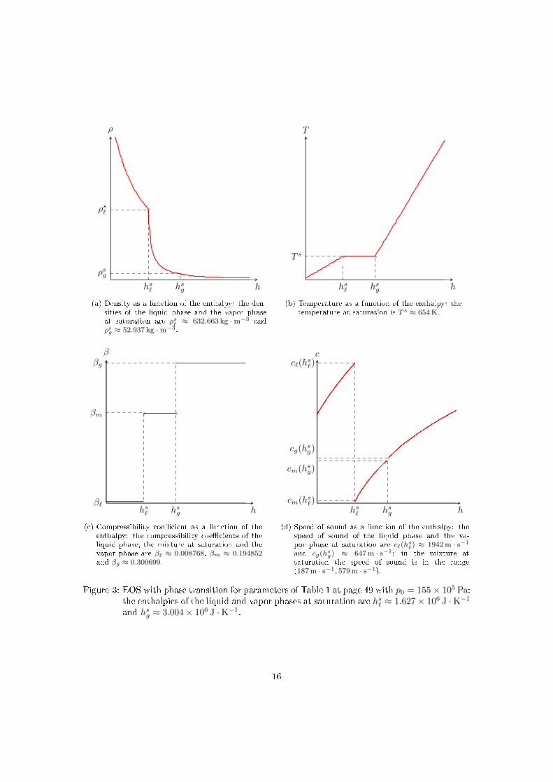
h

ρ

ρs`

hs`

ρsg

hsg

(a) Density as a function of the enthalpy: the den-sities of the liquid phase and the vapor phaseat saturation are ρs` ≈ 632.663 kg ·m−3 andρsg ≈ 52.937 kg ·m−3.

h

T

T s

hsghs`

(b) Temperature as a function of the enthalpy: thetemperature at saturation is T s ≈ 654 K.

h

ββg

hsgβ`

βm

hs`

(c) Compressibility coe�cient as a function of theenthalpy: the compressibility coe�cients of theliquid phase, the mixture at saturation and thevapor phase are β` ≈ 0.008768, βm ≈ 0.194852and βg ≈ 0.300699.

h

c

cg(hsg)

hsg

cm(hsg)

c`(hs`)

hs`

cm(hs`)

(d) Speed of sound as a function of the enthalpy: thespeed of sound of the liquid phase and the va-por phase at saturation are c`(hs`) ≈ 1942 m · s−1

and cg(hsg) ≈ 647 m · s−1; in the mixture atsaturation the speed of sound is in the range(187 m · s−1, 579 m · s−1).

Figure 3: EOS with phase transition for parameters of Table 1 at page 49 with p0 = 155× 105 Pa:the enthalpies of the liquid and vapor phases at saturation are hs` ≈ 1.627× 106 J ·K−1

and hsg ≈ 3.004× 106 J ·K−1.

16

3.1. Validity of the model

As stated in � 2.3, we must ensure of the positivity of h − q(h, p0) for h solution to (2.17). Wemention that in the framework of sti�ened gas satisfying (2.8), Hypotheses 1.2(2.) and 1.4(2.)reduce to:

Hypothesis 3.1. Data he and h0 are such that

H def= min

{inft≥0

he(t), miny∈[0,L]

h0(y)

}> q`.

Indeed, if at instant t the inlet �ow is in liquid phase (i.e. he(t) < hs`) and satis�es Hypothesis 3.1,then he(t) − q(he(t), p0) = he(t) − q` > 0. If the inlet �ow is a mixture of liquid and steam(i.e. he(t) ∈ [hs` , h

sg]), then he(t) − q(he(t), p0) = he(t) − qm ≥ hs` − qm > 0 according to

(2.15). Likewise, if the inlet �ow is in vapor phase (i.e. he(t) > hsg), then he(t)− q(he(t), p0) =he(t)− qg > hsg − qg > 0 according to (2.15). Thus, in each case, he(t)− q(he(t), p0) > 0 whichimplies that ρe(t) is well-de�ned and positive through (2.8) and (2.12a). The same proof appliesto h0.

To go further, we need to de�ne some notations that will be useful for the whole section. Tosolve the transport equation (2.17), we make use of the method of characteristics. This methodconsists in constructing curves (called characteristic curves) along which PDE (2.17) reduces toan ordinary di�erential equation (ODE). More precisely, let χ(τ ; t, y) be the position at time τof a particle located in y at time t in a �ow driven at velocity v. For t ≥ 0 and y ∈ (0, L), χ isthus solution to the parametrized ODE

dχ

dτ(τ ; t, y) = v

(τ, χ(τ ; t, y)), (3.1a)

χ(t; t, y) = y. (3.1b)

The curve(τ, χ(τ ; t, y)

)is the characteristic curve passing through the point (t, y). Properties

of χ depend on the smoothness of the velocity �eld v.

We denote in the sequel (see Figure 4) ξ(t, y) the foot of the characteristic curve, t∗(t, y) thetime at which the characteristic curve crosses the boundary y = 0 and y∗(t) the location at timet of a particle initially placed at y = 0. In other words, ξ, t∗ and y∗ are de�ned by

ξ(t, y) def= χ(0; t, y), χ(t∗(t, y); t, y

)= 0 and ξ

(t, y∗(t)

)= 0. (3.2)

We thus have the characterization

ξ(t, y) > 0 ⇐⇒ t∗(t, y) < 0 ⇐⇒ y > y∗(t).

This enables to prove the following result:

Lemma 3.1. When Hypothesis 3.1 is satis�ed, any smooth solution to PDE (2.17) with BC(1.3a) and well-prepared initial conditions satis�es h− q(h, p0) > 0.

Proof of Lemma 3.1. We recall that q is de�ned through (2.14). For any t ≥ 0 and y ∈ (0, L),there are three possible situations:

� If h(t, y) > hsg, then h(t, y)− q(h(t, y), p0

)> hsg − qg > 0 because of (2.15);

17

� If h(t, y) ∈ [hs` , hsg], then h(t, y)− q

(h(t, y), p0

)≥ hs` − qm > 0 because of (2.15);

� If h(t, y) < hs` , then equation (2.17) reads (at least locally by a smoothness argument)

∂t(h− q`) + v∂y(h− q`) =β`Φ

p0(h− q`).

We infer that h : (τ ; t, y) 7→ h(τ, χ(τ ; t, y)

)satis�es

∂τ

[h(τ ; t, y)− q`

]=[h(τ ; t, y)− q`

] β`p0

Φ(τ, χ(τ ; t, y)

),

h(t; t, y) = h(t, y).

Hence

h(t, y)− q` =[h(τ ; t, y)− q`

]exp

(β`p0

∫ t

τ

Φ(σ, χ(σ; t, y)

)dσ

)for any τ such that χ(τ ; t, y) ∈ (0, L).

This shows that h(t, y)− q` is continuous and has the same sign

? as he(t∗(t, y)

)− q` (if ξ(t, y) ≤ 0),

? or as h0

(ξ(t, y)

)− q` (if ξ(t, y) ∈ [0, L]),

? or as hs` − q` (if ξ(t, y) > L or if ξ(t, y) does not exist, i.e. when phase change occursbefore and after).

All of them are positive thanks to Hypothesis 3.1 and (2.15).

3.2. Exact and asymptotic solutions for single-phase �ow

In this section, we compute some analytical solutions of (1.1) supplemented with the sti�enedgas law for some particular cases (according to relevant values for Φ, he and De) when a singlephase κ ∈ {`,m, g} is present. The compressibility coe�cient β and the coe�cient q are thusconstant.

Since we focus on the 1D case and as βκ(h, p0) = βκ in the case of the sti�ened gas law, we cancompute the velocity v by a direct integration of equation (1.1a), which gives

v(t, y) = ve(t) +βκp0

∫ y

0

Φ(t, z) dz, (3.3)

with ve de�ned by (1.4). This velocity is obviously nonnegative under Hypotheses 1.1, 1.2 and1.3, so that it is compatible with the location of BC. As mentioned earlier, equation (1.1b) canbe rewritten as (2.17). To compute the enthalpy, we apply the method of characteristics (seeabove) which gets simpler in the case of the sti�ened gas law.

The following results had �rst been stated in [6]. The proofs are detailed below.

18

yL

t

ξ( t 1, y∗ (t 1

)) =

0

t1

y∗(t1)

ξ(t 1, y

1) y1

t∗

ξ(t 1, y

2) y2

Figure 4: Sketch of the method of characteristics and de�nitions of ξ(t, y), t∗(t, y) and y∗(t).

3.2.1. Constant power density

Proposition 3.1. Let us assume that

� the power density Φ = Φ0 > 0 is constant in time and space;

� he and De satisfy Hypotheses 1.2 and 3.1 and are such that ve = De/ρ(he, p0) is indepen-dent of time;

� h0 veri�es Hypotheses 1.4 and 3.1.

Let us denote Φ0def= βκΦ0/p0. Then ξ(t, y) and t∗(t, y) de�ned by (3.2) are equal to

ξ(t, y) =

(y +

ve

Φ0

)e−Φ0t − ve

Φ0

,

t∗(t, y) = t− 1

Φ0

ln

(1 +

Φ0

vey

)= − 1

Φ0

ln

(1 +

Φ0

veξ(t, y)

),

and the solution h of equation (1.1b) supplemented with BC (1.3a) is given by

h(t, y) =

qκ +

[h0

(ξ(t, y)

)− qκ

]eΦ0t, if ξ(t, y) ≥ 0,

qκ +[he(t∗(t, y)

)− qκ

](1 +

Φ0y

ve

)= he

(t∗(t, y)

)+

Φ0y

De

(t∗(t, y)

) , if ξ(t, y) < 0.

(3.4)

Corollary 3.1. Under the hypotheses of Prop. 3.1, we have y∗(t) = (eΦ0t−1) veΦ0

and the solution

p of equation (1.1c) together with BC (1.3c) is given by

� if y∗(t) > L, then

p(t, y) = Φ0[µ(y)− µ(L)]+

vep0

βκ

{g[He

(t∗(t, y)

)−He

(t∗(t, L)

)]+ Φ0vee

Φ0t[He

(t∗(t, y)

)−He

(t∗(t, L)

)]}; (3.5a)

19

� if y∗(t) ≤ L and y ≥ y∗(t) then

p(t, y) = Φ0[µ(y)− µ(L)]+

p0

βκ

{(g + Φ0vee

Φ0t) [H0

(ξ(t, L)

)−H0

(ξ(t, y)

)]+ Φ2

0eΦ0t[H0

(ξ(t, L)

)−H0

(ξ(t, y)

)]}; (3.5b)

� otherwise

p(t, y) = Φ0[µ(y)− µ(L)]+

p0

βκ

{(g + Φ0vee

Φ0t) [H0

(ξ(t, L)

)−H0(0)

]+ Φ2

0eΦ0t[H0

(ξ(t, L)

)−H0(0)

]+ ve

{g[He

(t∗(t, y)

)−He(0)

]+ Φ0vee

Φ0t[He

(t∗(t, y)

)−He(0)

]}}; (3.5c)

where H′0(y) = 1/(h0(y) − qκ), H

′0(y) = y/(h0(y) − qκ), H

′e(t) = 1/(he(t) − qκ) and H

′e(t) =

e−Φ0t/(he(t)− qκ).

Notice that Equation (3.5c) is a correction of Equation (9b) in [6].

Remark 3.1. As it has been stated in [6], if the inlet enthalpy is also constant and if the inletvelocity is nonzero, there is an asymptotic state which is reached in �nite time. This time isequal to t∞ = 1

Φ0ln(1 + Φ0L

ve) and satis�es ξ(t∞, L) = 0 and y∗(t∞) = L. Hence, for t ≥ t∞, the

solution (h, v, p)(t, y) is given by

h∞(y) = he +Φ0

Dey,

v∞(y) = ve + Φ0y,

p∞(y) = Φ0[µ(y)− µ(L)] +gDe

Φ0

ln

1 + Φ0Lve

1 + Φ0yve

+ Φ0De(L− y).

However, if the inlet velocity is ve = 0, then ξ(t, y) is always positive and no asymptotic statecan be reached since the enthalpy increases continuously in time.

Remark 3.2. Proposition 3.1 applies for nonzero Φ0. When Φ0 = 0, the same proof holds exceptthe resolution of ODE (3.1) whose solution becomes χ(τ ; t, y) = y + ve(τ − t). We remark thatsolution (3.7) converges to this case when Φ0 → 0, which shows that the model is continuous withrespect to Φ0. In particular, the enthalpy reads

h(t, y) =

{h0(y − vet), if y ≥ vet,he(t− y/ve), otherwise,

which was expected as h is a solution to a simple linear transport equation.

20

Proof of Proposition 3.1. Equation (3.3) becomes

v(t, y) = ve + Φ0y. (3.6)

Since v is linear, the Cauchy-Lipschitz theorem applied to ODE (3.1) ensures the existence of χover some interval (depending on t and y). Moreover, χ is continuous with respect to (τ, t, y).We then solve ODE (3.1) using expression (3.6). We obtain

χ(τ ; t, y) =

(y +

ve

Φ0

)eΦ0(τ−t) − ve

Φ0

. (3.7)

For �xed t ≥ 0 and y ∈ (0, L), the requirement χ(τ ; t, y) ∈ (0, L) constrains the interval ofexistence

τ ∈

max {0; t∗(t, y)} , t+1

Φ0

ln

1 + Φ0Lve

1 + Φ0yve

. (3.8)

For (τ, t, y) satisfying (3.8), we note

h(τ ; t, y) def= h(τ, χ(τ ; t, y)

). (3.9)

We deduce from equation (1.1b) rewritten under the form equation (2.17) that h satis�es{∂τ

[h(τ ; t, y)− qκ

]= Φ0

[h(τ ; t, y)− qκ

],

h(t; t, y) = h(t, y).

The solution of this linear �rst order ODE is

h(t, y)− qκ = h(t; t, y)− qκ =[h(τ ; t, y)− qκ

]eΦ0(t−τ) =

[h(τ, χ(τ ; t, y)

)− qκ

]eΦ0(t−τ). (3.10)

Two cases must be investigated depending on the minimal time until which the characteristiccurve remains in the domain or equivalently depending on the sign of ξ (see (3.8) and Figure 4):

� if ξ(t, y) ≥ 0, then the characteristic curve does not cross the boundary y = 0, which meansthat we can take τ = 0 in equation (3.10) and

h(t, y)− qκ =[h0

(χ(0; t, y)

)− qκ

]eΦ0t =

[h0

(ξ(t, y)

)− qκ

]eΦ0t;

� if ξ(t, y) < 0, the backward characteristic curve reaches the boundary at time t∗(t, y) > 0and

h(t, y)− qκ = [he(t∗)− qκ]eΦ0(t−t∗) = [he(t

∗)− qκ]

(1 +

Φ0y

ve

).

Noticing that βκp0

(h− qκ) = 1ρ leads to

h(t, y) = qκ + [he(t∗)− qκ] +

1

ρe(t∗)

Φ0

vey = he(t

∗) +Φ0

De(t∗)y.

21

Proof of Corollary 3.1. The exact dynamic pressure p can be computed by integrating the mo-mentum equation (1.1c) which is equivalent to

∂yp = −∂t(ρv)− ∂y(ρv2) + ∂y(µ∂yv)− ρg.

Using the mass conservation law and observing that v given by (3.6) is independent of time, weobtain

∂yp = −(Φ0v + g)ρ+ Φ0∂yµ

from which we deduce

∂yp = − p0

βκ

g + Φ0(ve + Φ0y)

h− qκ+ Φ0∂yµ.

Integrating between y and L, we get due to BC (1.3c)

p(t, y) =p0(g + Φ0ve)

βκ

∫ L

y

1

h(t, z)dz +

p0Φ20

βκ

∫ L

y

z

h(t, z)dz + Φ0[µ(y)− µ(L)] (3.11)

where h def= h− qκ. Since h is de�ned piecewise by (3.4), we have to consider three cases:

� If y∗(t) > L, the curve τ 7→ χ(τ ; t, y) lies in the green part of the graph on Figure 4, i.e.above the curve τ 7→ χ

(τ ; t, y∗(t)

). As y∗(t) > L =⇒ χ(t, y) < 0 for all (t, y) ∈ R+× (0, L),

we can select the relevant value for h in (3.4), i.e. h(t, y) = he(t∗(t, y)

) (1 + Φ0y

ve

).

To compute each integral in (3.11), we use the change of variables τ = t∗(t, z), which yields∫ L

y

1

h(t, z)dz = −ve

∫ t∗(t,L)

t∗(t,y)

1

he(τ)dτ = ve

[He(τ)

]t∗(t,y)

t∗(t,L),∫ L

y

z

h(t, z)dz =

v2e

Φ0

∫ t∗(t,y)

t∗(t,L)

eΦ0(t−τ) − 1

he(τ)dτ =

v2e

Φ0

[eΦ0tHe(τ)−He(τ)

]t∗(t,y)

t∗(t,L).

We then infer (3.5a).

� If y∗(t) ≤ L and y ≥ y∗(t) (=⇒ ξ(t, y) ≥ 0), we have h(t, y) = h0

(ξ(t, y)

)eΦ0t so that by

means of the change of variable ζ = ξ(t, z) we specify the integrals in (3.11)∫ L

y

1

H(t, z)dz =

∫ ξ(t,L)

ξ(t,y)

1

h0(ζ)dζ =

[H0(ζ)

]ξ(t,L)

ξ(t,y),∫ L

y

z

h(z)dz = eΦ0t

∫ ξ(t,L)

ξ(t,y)

ζ

h0(ζ)dζ + (eΦ0t − 1)

ve

Φ0

∫ ξ(t,L)

ξ(t,y)

1

h0(ζ)dζ

= eΦ0t[H0(ζ)

]ξ(t,L)

ξ(t,y)+ (eΦ0t − 1)

ve

Φ0

[H0(ζ)

]ξ(t,L)

ξ(t,y).

Hence we deduce (3.5b).

� The last corresponds to y < y∗(t) ≤ L. The integration domain is split into two partsdepending on the sign of ξ(t, z). More precisely∫ L

y

f(z) dz =

∫ L

y∗(t)

f(z) dz +

∫ y∗(t)

y

f(z) dz

for any function f . For integrals between y∗(t) and L, we apply Formula (3.5b) withy = y∗(t). For integrals between y and y∗(t), we apply Formula (3.5a) with L replaced byy∗(t). Summing all terms leads to (3.5c).

22

3.2.2. Varying power density (with y or t)

Let us generalize the results of Proposition 3.1 by taking Φ = Φ(y):

Proposition 3.2. Let us assume that

� the power density Φ depends only on space;

� he and De satisfy Hypotheses 1.2 and 3.1 and are such that ve = De/ρ(he, p0) is indepen-dent of time;

� h0 veri�es Hypotheses 1.4 and 3.1.

Let us de�ne

Θ(y) def=

∫ y

0

dz

v(z)with v(z) = ve +

βκp0

∫ z

0

Φ(y) dy.

Then ξ and t∗ de�ned by (3.2) are equal to

ξ(t, y) = Θ−1(Θ(y)− t

)and t∗(t, y) = t−Θ(y).

The solution h of equation (1.1b) with BC (1.3a) is given by

h(t, y) =

qκ + v(y)

h0

(ξ(t, y)

)− qκ

v(ξ(t, y)

) , if ξ(t, y) ≥ 0,

qκ + v(y)he(t∗(t, y)

)− qκ

ve= he

(t∗(t, y)

)+

1

De

(t∗(t, y)

) ∫ y

0

Φ(z) dz, if ξ(t, y) < 0.

Let us note that v(y) = v0(y) since v(t, y) = v(y) and as v0 is well-prepared (see �1.2).

We can also extend the results of Proposition 3.1 by taking Φ = Φ(t):

Proposition 3.3. Let us assume that

� the power density Φ depends only on time;

� he and De satisfy Hypotheses 1.2 and 3.1;

� h0 veri�es Hypotheses 1.4 and 3.1.

Let us de�ne

Ψ(t) def=βκp0

∫ t

0

Φ(s) ds.

We thus have

ξ(t, y) = ye−Ψ(t) −∫ t

0

ve(s)e−Ψ(s)ds

and t∗(t, y) is the solution of the equation (upon t) y =

∫ t

t∗ve(s)e

Ψ(t)−Ψ(s)ds. Then the solution

h of equation (1.1b) with BC (1.3a) is given by

h(t, y) = qκ +

[h0

(ξ(t, y)

)− qκ

]eΨ(t), if ξ(t, y) ≥ 0,[

he(t∗(t, y)

)− qκ

]eΨ(t)−Ψ(t∗), if ξ(t, y) < 0.

23

Remark 3.3. In the general case, i.e. with time dependence for he and De and time/spacedependence for Φ, it does not seem possible to compute an exact solution. However, if he(t),De(t) and Φ(t, y) have a �nite limit as t → +∞ denoted by h∞e , D∞e , Φ∞(y), then there existsa steady solution for the enthalpy

h∞(y) = h∞e +1

D∞e

∫ y

0

Φ∞(z) dz

and all other quantities are deduced from h∞. We recover the result of [16].

Up to now, there is no theoretical result in the general case about the convergence of the unsteadysolution to this steady state. We just notice that solutions from Props. 3.2 and 3.3 actually do.

Proof of Proposition 3.2. Since the inlet velocity ve is a positive constant and as Φ does notdepend on t, the velocity v(t, y) = v(y) = v0(y) is a positive function independent of time due to(3.3). Function Θ introduced in the statement of Proposition 3.2 is thus invertible. In a similarway as for Proposition 3.1, we solve the characteristic ODE (3.1) which is equivalent to

1 =χ′

v(χ)= Θ′(χ)χ′ = [Θ(χ)]′.

For the sake of simplicity, we set χ′ = dχdτ and χ′′ = d2χ

dτ2 . This leads to Θ(χ(τ ; t, y)

)− Θ(y) =

Θ(χ(τ ; t, y)

)−Θ

(χ(t; t, y)

)= τ − t and

χ(τ ; t, y) = Θ−1(Θ(y) + τ − t

). (3.12)

We can ensure that χ(τ ; t, y) ∈ (0, L) provided τ ∈(max

{0, t∗(t, y)

}, t+ Θ(L)−Θ(y)

). Keeping

the same notation (3.9) for h, equation (2.17) becomes∂τ[h(τ ; t, y)− qκ

]=βκp0

[h(τ ; t, y)− qκ

]Φ(χ(τ ; t, y)

),

h(t; t, y) = h(t, y).

(3.13)

We di�erentiate ODE (3.1) to obtain

χ′′(τ ; t, y) = χ′(τ ; t, y)dv

dy

(χ(τ ; t, y)

)= χ′(τ ; t, y)

βκp0

Φ(χ(τ ; t, y)

).

The positivity of v implies that χ′(τ ; t, y) > 0 and

βκp0

Φ(χ(τ ; t, y)

)=χ′′(τ ; t, y)

χ′(τ ; t, y)=[ln(χ′(τ ; t, y)

)]′=[ln v(χ(τ ; t, y)

)]′.

Inserting this relation in equation (3.13), we have

∂τ (h− qκ) = (h− qκ)∂τ[ln v(χ(τ ; t, y)

)].

Hence

h(t, y)− qκ = v(y)h(τ, χ(τ ; t, y)

)− qκ

v(χ(τ ; t, y)

) .

24

Given expression (3.12) for χ, we �nally obtain

h(t, y) = qκ +

v(y)

h0

(ξ(t, y)

)− qκ

v(ξ(t, y)

) , if ξ(t, y) ≥ 0,

v(y)he(t∗(t, y)

)− qκ

ve, otherwise.

Proof of Proposition 3.3. As previously, the key point is the integration of the characteristicODE (3.1) which reads

d

dτ

(χ(τ)e−Ψ(τ)

)= ve(τ)e−Ψ(τ).

This leads to

χ(τ ; t, y) = yeΨ(τ)−Ψ(t) +

∫ τ

t

ve(s)eΨ(τ)−Ψ(s) ds.

Consequentlyh(t, y)− qκ =

[h(τ, χ(τ ; t, y)

)− qκ

]eΨ(t)−Ψ(τ).

The main issue is then to determine the interval for τ such that χ(τ ; t, y) ∈ (0, L). The equalityχ(τ ; t, y) = 0 can be rewritten as

y =

∫ t

τ

ve(s)eΨ(t)−Ψ(s) ds.

As the right hand side vanishes for τ = t, two cases may occur: either y is greater than the righthand side for τ = 0 (which would imply that the left bound of the interval is 0), or there existsτ = t∗ > 0 such that the previous equality holds. In the former case, we obtain

h(t, y)− qκ =[h0

(χ(0; t, y)

)− qκ

]eΨ(t),

while in the latter case

h(t, y)− qκ =[he(t∗(t, y)

)− qκ

]eΨ(t)−Ψ(t∗).

3.3. Exact and asymptotic solutions for two-phase �ow with phasetransition

In the case of a two-phase �ow with phase transition and if we can determine the position of eachphase, we can deduce the exact solution using the single-phase �ow results given in Section 3.2.In the particular case where all parameters and boundary/initial data are constant, the result isthe following.

25

ts`

ys`

tsg

ysg y

t

L

M

G

(a) Liquid (L), mixture (M) and vapor (G) re-gions of the spatiotemporal domain R+×R+

for the velocity.

ts`

ys`

tsg

ysg y

t

t`(y)

t m(y

)

tg(y)

(b) De�nition of four regions of the spatiotem-poral domain R+ × R+ for the enthalpy.

Figure 5: De�nition of regions for Proposition 3.4

Proposition 3.4. Let us assume that he(t) ≡ he > q`, ve(t) ≡ ve > 0, Φ(t, y) ≡ Φ0 andh0(y) ≡ h0 = he > q`. Let Φκ

def= βκΦ0/p0, where κ is respectively `, m, g in the liquid, mixtureand gas phases. We suppose that the initial and boundary data correspond to the liquid phase,i.e. he(= h0) < hs` . We set

ys`def=De

Φ0(hs` − he), ysg

def=De

Φ0(hsg − he).

Let us de�ne three curves in R+ × R+ as pictured on Figure 5b

t`(y) def=1

Φ`ln

(1 +

Φ`y

ve

), for 0 ≤ y ≤ ys` ,

tm(y) def=1

Φmln

(ve + (Φ` − Φm)ys` + Φmy

ve + Φ`ys`

)+ t`(y

s` ), for ys` < y < ysg,

tg(y) def=1

Φgln

(ve + (Φ` − Φm)ys` + (Φm − Φg)y

sg + Φgy

ve + (Φ` − Φm)ys` + Φmysg

)+ tm(ysg), for y ≥ ysg.

Let us also de�ne

ts`def= t`(y

s` ) =

1

Φ`ln

(hs` − q`h0 − q`

), tsg

def= tm(ysg) = ts` +1

Φmln

(hsg − qmhs` − qm

).

Then the spatiotemporal domain R+×R+ consists of three regions corresponding to liquid, mixtureand vapor phases as follows (see Figure 5a):

L ={

(t, y) ∈ R+ × R+∣∣ t ≤ ts` or y ≤ ys` } ,

M ={

(t, y) ∈ (ts` ,+∞)× (ys` ,+∞)∣∣ t ≤ tsg or y ≤ ysg

},

G ={

(t, y) ∈ (tsg,+∞)× (ysg,+∞)}

;

26

the solution v of equation (1.1a) is given by

v(t, y) =

ve + Φ`y, if (t, y) ∈ L,ve + Φ`y

s` + Φm(y − ys` ), if (t, y) ∈M,

ve + Φ`ys` + Φm(ysg − ys` ) + Φg(y − ysg), if (t, y) ∈ G,

and the solution h of equation (1.1b) is given by (see Figure 5b)

h(t, y) =

q` + (h0 − q`)eΦ`t, if (t, y) ∈ L and t < t`(y),

qm + (hs` − qm)eΦm(t−ts`), if (t, y) ∈M and t < tm(y),

qg + (hsg − qg)eΦg(t−tsg), if (t, y) ∈ G and t < tg(y),

he + Φ0

Dey, otherwise.

Remark 3.4. We notice that constant Φm is the Zuber's characteristic reaction frequency de�nedin [44] and used in [26]. Contrary to the latter paper, we do not assume the pure phases to beincompressible. Thus we can extend the Zuber's frequency to liquid and gas phases as a piecewiseconstant function.

Remark 3.5. In any case, we observe that a steady state is reached. It is given by

h∞(y) = he +Φ0

Dey

and the velocity is piecewise linear. Moreover, we can determine the time t∞ at which the steadystate (it is thus an asymptotic state in that case) is reached

t∞ def=

t`(L), if ys` > L,

tm(L), if ys` ≤ L ≤ ysg,tg(L), if ysg < L.

The assumptions of Proposition 3.4 may seem restrictive but it can be trivially extended toseveral cases:

� to other constant initial and boundary conditions (i.e. mixture or vapor);

� if Φ = Φ0 < 0 such that v remains positive, the enthalpy is then still monotone.

If Φ and/or boundary-initial conditions are not constant anymore, the enthalpy is no longermonotone. It is thus di�cult to determine regions L,M and G. However, if this can be achieved,we can similarly apply the monophasic results in each region to compute the exact solution. Inany case, the following result holds (similar to Remark 3.3):

Remark 3.6. For any inlet velocity ve, inlet �ow rate De and power density Φ which have �nitelimits in time, let us denote

(h∞e , D

∞e ,Φ

∞(y))

= limt→+∞

(he(t), De(t),Φ(t, y)

). Then, there exists

a steady solution(h∞(y), v∞(y), p∞(y)

)given by

h∞(y) = h∞e +1

D∞e

∫ y

0

Φ∞(z) dz,

v∞(y) =D∞e

ρ(h∞(y), p0

) ,

27

p∞(y) = g

∫ L

y

ρ(h∞(z), p0

)dz −

[µβ(h∞(z), p0

)Φ∞(z)

p0− (D∞e )

2

ρ(h∞(z), p0

)]z=Lz=y

,

with ρ(h∞, p0) given by (2.3).

Proof of Proposition 3.4. Since ρe, ve, h0 and Φ0 are constant and correspond to the liquid phase,equations (1.1a)-(2.17) are written over a time interval [0, T ) for some T > 0 to be speci�ed later(which corresponds to the �rst time another phase appears)

∂yv = Φ`,

∂th+ v∂yh = Φ`(h− q`),v(t, 0) = ve,

h(t, 0) = he,

h(0, x) = h0 = he.

We can apply Proposition 3.1 to this system which leads to

v(y) = ve + Φ`y

and

h(t, y) =

q` + (h0 − q`)eΦ`t, if t < t`(y),

he +Φ0

Dey, otherwise,

where the curve t = t`(y) corresponds to the characteristic curve coming from (t = 0, y = 0), thatis ξ`(t, y) = 0 (see Proposition 3.1 for the de�nition of ξ`). The enthalpy h(t, ·) is a monotone-increasing function consisting (spatially) of a linear part and a constant part at each time. Twosituations may occur:

� either he + Φ0

DeL ≤ hs` : the �uid remains liquid inde�nitely (T = +∞) and the enthalpy is

equal to he + Φ0

Dey everywhere as soon as t ≥ t`(L);

� or he + Φ0

DeL > hs` : a mixture phase appears.

In the latter case, there exists t > 0 and y ∈ (0, L) such that h(t, y) = hs` . We then de�ne T = ts`as the solution of h(ts` , L) = hs` and y

s` as the smallest y such that h(ts` , y) = hs` , i.e.

q` + (h0 − q`)eΦ`ts` = hs` , he +

Φ0

Deys` = hs` .

For t > ts` , the �uid is in liquid phase for y < ys` and in mixture phase for y ≥ ys` and t smallenough, i.e. t ∈ [ts` , T ′). Therefore, in the liquid region the previous solution is still valid,whereas in the mixture region [ts` , T ′)× [ys` , L] equations (1.1a)-(2.17) are written as

∂yv = Φm,

∂th+ v∂yh = Φm(h− qm),

v(t, ys` ) = ve + Φ`ys` ,

h(t, ys` ) = hs` ,

h(ts` , y) = hs` .

28

y2 yN−1

hnivnipni

yi

0

y1

hn1 =he(tn)

vn1 =ve(tn)

L

yN

pnN = p0

Figure 6: Grid and boundary conditions.

We adapt Proposition 3.1 to the current spatiotemporal domain so that we obtain

v(y) = ve + Φ`ys` + Φm(y − ys` )

and

h(t, y) =

qm + (hs` − qm)eΦm(t−ts`), if t < tm(y),

he +Φ

Dey, otherwise.

The curve t = tm(y) corresponds to the characteristic curve passing through (ts` , ys` ), i.e.

tm(y) =1

Φmln

(ve + (Φ` − Φm)ys` + Φmy

ve + Φ`ys`

)+ ts` .

This can be rewritten in a simpler form. To this end, we use the de�nition of ys` , the relation1ρe

= β`p0

(he− q`) and the continuity of ρ at ys` (implying βm(hs` − qm) = β`(hs` − q`)) which leads

to

tm(y) =1

Φmln

(he − qm + Φ0y

De

hs` − qm

)+ ts` .

If needed, we apply the same procedure to �nd (tsg, ysg) such that hsg is reached and the proof

follows.

4. Numerical scheme

The main advantage of dimension 1 is that equations in (1.1) can be decoupled in an explicitnumerical procedure which means that it su�ces to compute h from equation (1.1b) � i.e. (2.17)for the sti�ened gas law � in order to deduce all other variables. To solve the transport equationwith source term (2.17), the numerical method of characteristics (MOC) seems suitable insofaras this method was essential in the theoretical part of the study. Moreover, this method hasinteresting properties such as unconditional stability and positivity-preserving for variable h− q(see � 4.3). Accuracy can be improved using 2nd-order results from [38].

Given ∆y > 0 and ∆t > 0, we consider a uniform Cartesian grid { yi = i∆y }1≤i≤N such thaty1 = 0 and yN = L (see Figure 6) as well as a time discretization { tn = n∆t }n≥0. Unknownsare collocated at the nodes of the mesh. We set the initial values v0

i = v0(yi) and h0i = h0(yi)

for i = 1, . . . , N .

29

We must emphasize that as the pressure variable p is supposed to be constant and equal to p0

in the Lmnc model, most parameters are constant throughout the study (such as T s, βκ or qκ).That is why references to the dependence on the pressure may be dropped in the sequel for thesake of simplicity.

4.1. Key idea of the scheme

For details about numerical methods of characteristics, the reader may refer to [2, 20, 38] andreferences therein. This method amounts to tracking particles along the �ow and to solve ODEsalong the characteristic curves. More precisely, it consists in locating accurately the position ofparticles and updating the unknown according to the source term as described from a theoreticalpoint of view in Section 3.2. Actually, at time tn, we aim at approximating the solution of

d

dτhn+1i (τ) =

β(hn+1i (τ)

)Φ(τ, χ(τ ; tn+1, yi)

)p0

(hn+1i (τ)− q

(hn+1i (τ)

)), (4.1a)

where τ 7→ hn+1i (τ) def= h

(τ, χ(τ ; tn+1, yi)

)and the characteristic �ow χ satis�es

d

dτχ(τ ; tn+1, yi) = v

(τ, χ(τ ; tn+1, yi)

), τ ≤ tn+1,

χ(tn+1; tn+1, yi) = yi,

(4.1b)

with v an approximate solution to (1.1a). The reader may refer to [38] for further details aboutthe resolution of (4.1b).

The classic Euler-type MOC method applied to ODE (4.1a) over the interval [tn; tn+1] is writ-ten

h(tn+1, yi) = hn+1i (tn+1)

= hn+1i (tn) + ∆t

β(hn+1i (tn)

)Φ(tn, χ(tn; tn+1, yi)

)p0

(hn+1i (tn)− q

(hn+1i (tn)

))+O(∆t2).

Hence the scheme can be written

hn+1i = hn+1,n

i + ∆tβ(hn+1,ni

)Φ(tn, ξni

)p0

(hn+1,ni − q

(hn+1,ni

)), (4.2)

where ξni and hn+1,ni are some approximations of χ(tn; tn+1, yi) and hn+1

i (tn) respectively. Inthe sequel, scheme (4.2) will be referred to as the MOC scheme.

To reach higher order, we rewrite ODE (4.1a) using the facts that β(h) and h− q(h) are positiveunder Hypotheses 1.3 and 3.1. We set

R(h) def=

∫ h

H

dh

β(h) ·(h− q(h)

) ,where H is de�ned within Hypothesis 3.1. Then, equation (4.1a) reads

R′(hn+1i

) d

dτhn+1i (τ) =

Φ(τ, χ(τ ; tn+1, yi)

)p0

(4.3)

30

and thus can be integrated explicitly between tn and tn+1

R(hn+1i (tn+1)

)−R

(hn+1i (tn)

)=

1

p0

∫ tn+1

tnΦ(τ, χ(τ ; tn+1, yi)

)dτ.

As Φ is a datum, the right hand side can be expanded at any order or exactly computed. Usingthe trapezoidal rule, the scheme reads

hn+1i = R−1

(R(hn+1,ni

)+

∆t

p0

Φ(tn, ξni ) + Φ(tn+1, yi)

2

). (4.4)

Notice that we can give explicit expressions for R and R−1:

R(h) =

1β`

ln(h−q`H−q`

), if h ≤ hs` ,

Rs` + 1βm

ln(h−qmhs`−qm

), if hs` < h < hsg,

Rsg + 1βg

ln(h−qghsg−qg

), if h ≥ hsg,

R−1(r) =

q` + (H− q`)eβ`r, if r ≤ Rs` ,qm + (hs` − qm)eβm(r−Rs`), if Rs` < r < Rsg,

qg + (hsg − qg)eβg(r−Rsg), if r ≥ Rsg,

where

Rs`def=

1

β`ln

(hs` − q`H− q`

), Rsg

def=Rs` +1

βmln

(hsg − qmhs` − qm

).

Strategy (4.4) is named INTMOC. We recall that hsκ > qκ and hsg > hs` > qm � see (2.15) � andthat H > q` under Hypothesis 3.1. Thus, Rs` and R

sg are well-de�ned.

Strategies (4.2) and (4.4) being set up, it remains to specify how to compute ξni and hn+1,ni .

These computations are the core of numerical methods of characteristics and are detailed in thenext section.

4.2. Description of the scheme

Given the numerical solutions (hni , vni , p

ni ), the overall process at step n+ 1 consists in computing

successively hn+1i , vn+1

i and pn+1i as follows.

• Enthalpy. For the boundary condition (i = 1) we impose hn+11 = he(t

n+1). Then hn+1i is

determined in two steps:

¬ Solve ODE (4.1b) over the interval [tn, tn+1]. The approximation ξni of χ(tn; tn+1, yi)is computed either at order 1 or 2:

(i) at order 1 in time, we have χ(tn; tn+1, yi) ≈ yi −∆t · v(tn, yi) so that we set

ξni = yi −∆t · vni ; (4.5)

31

(ii) at order 2 in time (see [38,39] for more details), we have

χ(tn; tn+1, yi) ≈ yi −∆t · v(tn, yi)−1

2∆t2

(∂tv(tn, yi)− v(tn, yi)∂yv(tn, yi)

).

Due to (1.1a) and with a standard 1st-order �nite-di�erence discretization for∂tv, we set

ξni = yi −∆t

(3

2vni −

1

2vn−1i

)+

∆t2

2

β(hni )

p0vni Φ(tn, yi). (4.6)

­ Update the enthalpy:

� if ξni > 0 (see Figure 7a), let j be the index such that ξni ∈ [yj , yj+1) andθnij

def=(yj+1 − ξni )/∆y. As ξni is generally not a mesh node, we use an interpo-

lation procedure to evaluate hn+1,ni :

(i) at order 1hn+1,ni = θnijh

nj + (1− θnij)hnj+1; (4.7)

(ii) at higher order (see [38] for more details)

hn+1,ni = λni h

−j + (1− λni )h+

j (4.8)

where

λnidef=

1+θnij

3 , if P+j (θnij) ≥ 0 and P−j (θnij) ≥ 0,

0, if P+j (θnij) ≥ 0 and P−j (θnij) < 0,

1, if P+j (θnij) < 0 and P−j (θnij) ≥ 0,

θnij , otherwise,

h−jdef=

hnj , if P+

j (θnij) < 0 and P−j (θnij) < 0,

(θnij)2

2

(hnj−1 − 2hnj + hnj+1

)−θnij2

(hnj−1 − 4hnj + 3hnj+1

)+ hnj+1,

otherwise,

h+j

def=

hnj+1, if P+

j (θnij) < 0 and P−j (θnij) < 0,

(θnij)2

2

(hnj+2 − 2hnj+1 + hnj

)−θnij2

(hnj+2 − hnj

)+ hnj+1,

otherwise,

and P±j (θ) def=(θ − δ±j )(θ − δ±j+1) with

δ−jdef=

2(hnj+1 − hnj )

hnj−1 − 2hnj + hnj+1

, δ+j

def=2(hnj+1 − hnj )

hnj − 2hnj+1 + hnj+2

,

δ−j+1def=hnj−1 − 4hnj + 3hnj+1

hnj−1 − 2hnj + hnj+1

, δ+j+1

def=hnj+2 − hnj

hnj − 2hnj+1 + hnj+2

.

32

y

t

yj−1 yj yj+1

tn+1

yi

tn

ξni

(a) ξni > 0

y

t

0

tn+1

yi

tn

ξni

t∗i

(b) ξni ≤ 0

Figure 7: Numerical method of characteristics.

This procedure has been designed in [38] in order to ensure the maximum prin-ciple by means of a variable stencil (and an adaptive order). Even if there isno maximum principle associated to equation (2.17), this scheme preserves theproperty hni − q(hni ) > 0 (see Proposition 4.1).

We then update hn+1i by formulae (4.2) or (4.4).

� if ξni ≤ 0 (see Figure 7b), we compute the time t∗i at which the characteristic curveτ 7→ χ(τ ; tn+1, yi) crosses the in�ow boundary. There we have h(t∗i , 0) = he(t

∗i ).

Using a �rst order approximation in time, we set t∗i = tn+1 − yi/vni and we

compute the updated enthalpy similarly to what is detailed above:

(i) by integrating ODE (4.1a) over [t∗i , tn+1] (MOC strategy)

hn+1i = he(t

∗i ) + (tn+1 − t∗i )

β(he(t

∗i ))Φ(t∗, 0)

p0

[he(t

∗i )− q

(he(t

∗i ))]

; (4.9a)

(ii) by integrating ODE (4.3) over [t∗i , tn+1] (INTMOC strategy)

hn+1i = R−1

(R(he(t

∗i ))

+tn+1 − t∗i

p0

Φ(t∗i , 0) + Φ(tn+1, yi)

2

). (4.9b)

The boundary y = 0 is the only one we need to care about since characteristic curvescannot exit from the domain at y = L (we assumed that ve > 0 and Φ ≥ 0 which impliesthat v > 0).

• Velocity. For the boundary condition (i = 1), we set vn+11 = ve(t

n+1). Then, we integrateequation (1.1a) over [yi, yi+1]. Depending on the ability to compute the primitive functionof Φ (and as β is piecewise constant), the velocity �eld can be computed directly

vn+1i = vn+1

i−1 +1

p0

∫ yi

yi−1

β(h(tn+1, z)

)Φ(tn+1, z) dz, (4.10)

or approximated for example by the following upwind approach

vn+1i = vn+1

i−1 +∆y

p0β(hn+1

i−1 )Φ(tn+1, yi−1) (4.11)

33

since h is transported by vni ≥ 0. However, since the coe�cient β is discontinuous at phasechange points (see Figure 3c), we have to adapt the previous algorithm in cells where the�uid changes from a phase to the mixture. It is reasonable to suppose that at most apure phase and a mixture are present within a single cell (never liquid, mixture and steamsimultaneously). Then, if hsκ ∈ (hn+1

i−1 , hn+1i ), let y∗ be the linear approximation of ysκ, i.e.

y∗ def= yi−1 + ∆yhsκ − hn+1

i−1

hn+1i − hn+1

i−1

.

Hence∫ yi

yi−1

β(h(tn+1, z)

)Φ(tn+1, z) dz

=

∫ y∗

yi−1

β(h(tn+1, z)

)Φ(tn+1, z) dz +

∫ yi

y∗β(h(tn+1, z)

)Φ(tn+1, z) dz (4.10')

or when the primitive function of Φ is not known∫ yi

yi−1

β(h(tn+1, z)

)Φ(tn+1, z) dz

≈ (y∗ − yi−1)β(hn+1i−1 )Φ(tn+1, yi−1) + (yi − y∗)β(hn+1

i )Φ(tn+1, yi). (4.11')

• Pressure. For the boundary condition (i = N), we set pnN = p0. Then we rewrite equa-tion (1.1c) in the following equivalent form

−∂yp = ∂t(ρ(h)v) + ∂y(ρ(h)v2)− ∂y(µ∂yv) + ρ(h)g

= ρ(h)∂tv + ρ(h)v∂yv − ∂y(µ∂yv) + ρ(h)g.

Using (1.1a) it becomes

−∂yp = ρ(h)∂tv + ρ(h)vβ(h)Φ

p0− ∂y

(µβ(h)Φ

p0

)+ ρ(h)g.

Let us note ρn+1i = ρ(hn+1

i ) and βn+1i = β(hn+1

i ). Integrating this equation over [yi−1, yi],we obtain

pn+1i−1 = pn+1

i +∆y

2

[(ρn+1i + ρn+1

i−1

)g + ρn+1

i

vn+1i − vni

∆t+ ρn+1

i−1

vn+1i−1 − vni−1

∆t

+ ρn+1i vn+1

i

βn+1i

p0Φ(tn+1, yi) + ρn+1

i−1 vn+1i−1

βn+1i−1

p0Φ(tn+1, yi−1)

]− µ

[βn+1i

p0Φ(tn+1, yi)−

βn+1i−1

p0Φ(tn+1, yi−1)

], i ∈ {2, . . . , N}.

(4.12)

4.3. Positivity-preserving property

We have the following result which is the discrete version of Lemma 3.1:

34

Proposition 4.1. When Hypothesis 3.1 is satis�ed, strategies (4.2)&(4.9a) and (4.4)&(4.9b)with well-prepared initial conditions ensure the positivity of hni − q(hni ) for any ∆t > 0.

Proof. For the sake of clarity, we set κ(h) the phase corresponding to the value of h, namelyκ(h) = ` if h < hs` , m if h ∈ [hs` , h

sg] and g if h > hsg. Let us show by induction the inequalities

hni ≥ H and hni > qκ(hni ). (4.13)

We recall that H is de�ned within Hyp. 3.1. Given the physical framework, we assume withoutloss of generality that the �uid is under the liquid phase initially and at the entry, which meanshe(t) < hs` and h0(y) < hs` for all t ≥ 0 and y ∈ (0, L). Estimates (4.13) is satis�ed for n = 0 byhypothesis. If it is satis�ed at iteration n, then hn+1,n

i ≥ H according to the maximum principleveri�ed by the interpolation processes (4.7) (by convexity) and (4.8) (by construction: see [38]).Then, if κ(hn+1,n

i ) ∈ {m, g}, we directly have hn+1,ni > qκ(hn+1,n

i ) due to (2.15). If κ(hn+1,ni ) = `,

then hn+1,ni ≥ H > q` due to Hyp. 3.1. To summarize, we have hn+1,n

i > qκ(hn+1,ni ).

To complete the proof, we remark that no matter what scheme is used to compute hn+1i from

hn+1,ni , the cases κ(hn+1

i ) ∈ {m, g} are trivially handled due to (2.15). It thus remains to dealwith κ(hn+1

i ) = `. If hn+1i is computed via the MOC scheme (4.2), as hn+1,n

i > qκ(hn+1,ni ), we

remark that hn+1i > hn+1,n

i , which implies that κ(hn+1,ni ) = `. Thus, (4.2) yields

hn+1i − q` = (hn+1,n

i − q`)(

1 + ∆tβ`Φ(tn, ξni )

p0

)> 0.

Likewise, if hn+1i is computed via the INTMOC scheme (4.4), as R−1 is monotone-increasing

owing to (2.15) and Hyp. 3.1, we have hn+1i > hn+1,n

i , which again implies that κ(hn+1,ni ) = `.

Scheme (4.4) then reads

hn+1i − q` = (hn+1,n

i − q`) exp

[∆t

β`(Φ(tn, ξni ) + Φ(tn+1, yi)

)2p0

].

Hence the conclusion, which also holds in the exiting characteristic curve case via schemes (4.9a)and (4.9b). Both schemes are thus compatible with our modelling of thermodynamics.

Both schemes (MOC and INTMOC) are explicit and unconditionally stable which are standard fea-tures for numerical methods of characteristics. The handling of boundary conditions is achievedin the present study at order 1. Although the time step can be chosen independently from themesh size, it must be small enough to provide accurate transient results.

5. Numerical examples

In this section, we focus on data sets for which phase transition occurs (for the simulations ofsingle-phase �ows, we refer to [6]).

To simulate some scenarii in a PWR, parameters are set as follows:

� Geometry of the reactor: L = 4.2 m;

35

� Discretization parameters: N = 100 mesh nodes (∆y ≈ 4.3 cm) and ∆t = 0.01 s;

� Reference value for the pressure, the power density and the velocity: p0 = 155× 105 Pa,Φ0 = 170× 106 W ·m−3, v = 0.5 m · s−1;

� Initial data: h0(y) = he, v0(y) = ve +∫ y

0β(h0(z))Φ(0, z)/p0dz (well-prepared insofar as

they satisfy the divergence constraint (1.1a));

� Constant viscosity: µ0 = 8.4 · 10−5 kg ·m−1 · s−1.

To perform simulations, we have to provide physical values for liquid and vapor sti�ened gasparameters. This is achieved by using the tables of water and steam [33] as described in theappendix C. Parameters involved in the sti�ened gas law for the following simulations are thosein Table 1, page 49. For this data set, variables at saturation are hs` ≈ 1.627× 106 J ·K−1,hsg ≈ 3.004× 106 J ·K−1, ρs` ≈ 632.663 kg ·m−3 and ρsg ≈ 52.937 kg ·m−3.

In Test 5.1, a two-phase �ow with phase transition is considered and enables to compare thenumerical schemes presented in Section 4, while all other tests only involve scheme (4.4)&(4.9b)with high order interpolation (4.8) (noted INTMOC_2) to assess the robustness of the scheme andthe relevance of the model.

5.1. Two-phase �ow with phase transition

In the �rst test, we investigate the ability of our model to deal with two-phase �ows withphase transition. We consider the case when the inlet density ρe, the inlet velocity ve, theinitial condition h0 and the power density Φ are constant, so that we can apply Proposition 3.4to compute exact transient and asymptotic solutions. The boundary conditions are ρe(t) =750 kg ·m−3 and ve(t) = v, thus h0(y) = he(t) = h`(ρe) ≈ 1.190× 106 J ·K−1. The powerdensity is set constant in space and time and equal to Φ0. With these parameters, the domain isinitially �lled with liquid. Then according to Proposition 3.4 mixture appears at time ts` ' 1.769 sfor y > ys` ' 0.964 m and pure vapor appears at time tsg ' 2.929 s for y > ysg ' 4.002 m. Theasymptotic state is reached at tg(L) ' 2.957 s.

Figure 8 displays numerical results for the enthalpy and the velocity at instants t = 2.1 s, t = 2.8 sand t = 3.5 s. At this last time the solution has already reached the asymptotic regime. Figure 9displays the mass fraction and the Mach number computed from the enthalpy and the velocity.Figure 10 displays the density and the temperature computed from the enthalpy.

In those �gures we compare the exact and asymptotic solutions to the di�erent versions of thenumerical scheme, namely:

� by scheme (4.2)&(4.9a) with linear interpolation (4.7) for hn+1,ni (called MOC_1),

� by scheme (4.2)&(4.9a) with high order interpolation (4.8) for hn+1,ni (called MOC_2),

� by scheme (4.4)&(4.9b) with linear interpolation (4.7) for hn+1,ni (called INTMOC_1),

� by scheme (4.4)&(4.9b) with high order interpolation (4.8) for hn+1,ni (called INTMOC_2).

We mention that the foot of the characteristic curve ξni is always computed by means of the2nd-order expression (4.6) and the velocity �eld by means of formulae (4.10) and (4.10').

We observe that all numerical results match the behaviour of the exact solution including phasetransition. Nevertheless as it can be noticed at time t = 2.8 s, there is some discrepancy close tothe singularity (interface between information coming from the boundary and the inner domain).

36

This can easily be accounted for. Indeed, the scheme relies on an interpolation process whichassumes some smoothness for the solution. As it is not smooth at the singularity, the schemeprovides a smoothened version of the exact solution. It must be underlined that the higher thedegree of interpolation, the more accurate the solution. Moreover, there is a clear advantage ofINTMOC versions of the scheme over MOC which is due to the better approximation of the righthand side in the former case. For these reasons, from now on, we will use only the INTMOC_2

scheme which is more accurate.

Figure 9 shows that the Mach number remains lower than 0.05 so that the low Mach numberhypothesis of the model is valid in this con�guration. Observe that during the transient state,the Mach number is greater than at the asymptotic state.

From a physical point of view, it is worth emphasizing that our model predicts the appearance ofsome vapor at the top of the reactor for this data set. This is due to a too small in�ow velocity.

5.2. Non monotone Φ

We perform a simulation for a steady power density piecewise constant in space

Φ(t, y) =

{Φ0, if y ≤ L/2,0, if y > L/2.

This power density models the situation where the control rods are blocked at the middle of thereactor. The boundary conditions are ρe(t) = 750 kg ·m−3 and ve(t) = v, thus h0(y) = he(t) =h`(ρe) ≈ 1.190× 106 J ·K−1. At the initial state the core thus is �lled with liquid, so that thevoid fraction is 0.

We emphasize that due to the steady boundary condition for the pressure and to the fact thatthe dynamic pressure is decoupled from the other variables in 1D, the right part [L/2, L] ofthe domain does not in�uence the left part [0, L/2]. This can also be seen in the statement ofProposition 3.4 where the process (for h and v) evolves from y = 0 to y = L. Hence, we canapply Proposition 3.4 over [0, L/2] since Φ is constant within. However, given the solution over[0, L/2] (and more speci�cally at y = L/2), we cannot apply Proposition 3.4 over [L/2, L] withthese inlet boundary conditions at y = L/2 as they are unsteady until the asymptotic state isreached. Besides, we know the global asymptotic solution which is given by Proposition 3.6.

We plot on Figure 11 the asymptotic solution from Proposition 3.6 and the numerical one com-puted by means of the INTMOC_2 scheme for the enthalpy, the mass fraction, the dynamicalpressure, the density and the temperature at the instants t = 0.0 s, t = 1.0 s, t = 2.0 s, t = 3.0 sand t = 4.0 s. The velocity is given at instants t < ts` , t = 1.8 s and t = 2.0 s. At t = ts` ' 1.768 smixture appears over [ys` , L/2] where ys` ' 0.964 m. This mixture is transported to �ll the do-main y ≥ ys` . As long as the domain is �lled with liquid, the velocity does not depend on time.When mixture appears, β is piecewise constant in the domain so that, according to Proposi-tion 3.4, the velocity increases up to the asymptotic value. The dynamical pressure is computedby scheme (4.12) and decreases towards the asymptotic state.

5.3. A simpli�ed scenario for a Loss of Flow Accident

Our model is tested here on an accidental transient regime: a main coolant pump trip whichis a Loss Of Flow Accident (LOFA) as at the beginning of the Fukushima accident in reactors

37

1e+06

1.2e+06

1.4e+06

1.6e+06

1.8e+06

2e+06

2.2e+06

2.4e+06

2.6e+06

2.8e+06

3e+06

3.2e+06

0 0.5 1 1.5 2 2.5 3 3.5 4

En

tha

lpy

y

t=2.100

MOC_1MOC_2

INTMOC_1INTMOC_2

ExactAsymptotic

0

1

2

3

4

5

6

7

8

0 0.5 1 1.5 2 2.5 3 3.5 4

Ve

locity

y

t=2.100

MOC_1MOC_2

INTMOC_1INTMOC_2

ExactAsymptotic

1e+06

1.2e+06

1.4e+06

1.6e+06

1.8e+06

2e+06

2.2e+06

2.4e+06

2.6e+06

2.8e+06

3e+06

3.2e+06

0 0.5 1 1.5 2 2.5 3 3.5 4

En

tha

lpy

y

t=2.800

MOC_1MOC_2

INTMOC_1INTMOC_2

ExactAsymptotic

0

1

2

3

4

5

6

7

8

0 0.5 1 1.5 2 2.5 3 3.5 4

Ve

locity

y

t=2.800

MOC_1MOC_2

INTMOC_1INTMOC_2

ExactAsymptotic

1e+06

1.2e+06

1.4e+06

1.6e+06

1.8e+06

2e+06

2.2e+06

2.4e+06

2.6e+06

2.8e+06

3e+06

3.2e+06

0 0.5 1 1.5 2 2.5 3 3.5 4

En

tha

lpy

y

t=3.500

MOC_1MOC_2

INTMOC_1INTMOC_2

ExactAsymptotic

0

1

2

3

4

5

6

7

8

0 0.5 1 1.5 2 2.5 3 3.5 4

Ve

locity

y

t=3.500

MOC_1MOC_2

INTMOC_1INTMOC_2

ExactAsymptotic

Figure 8: Numerical enthalpy (left) and velocity (right) for test 5.1: Two-phase �ow with phasetransition. We compare the four numerical solutions to the analytical and asymptoticones. The horizontal dotted lines correspond to h = hs` and h = hsg.

38

0

0.2

0.4

0.6

0.8

1

1.2

0 0.5 1 1.5 2 2.5 3 3.5 4

Ma

ss_

fra

ctio

n

y

t=2.100

MOC_1MOC_2

INTMOC_1INTMOC_2

ExactAsymptotic

0

0.02

0.04

0.06

0.08

0.1

0 0.5 1 1.5 2 2.5 3 3.5 4

Ma

ch

_n

um

be

r

y

t=2.100

MOC_1MOC_2

INTMOC_1INTMOC_2

ExactAsymptotic

0

0.2

0.4

0.6

0.8

1

1.2

0 0.5 1 1.5 2 2.5 3 3.5 4

Ma

ss_

fra

ctio

n

y

t=2.800

MOC_1MOC_2

INTMOC_1INTMOC_2

ExactAsymptotic

0

0.02

0.04

0.06

0.08

0.1

0 0.5 1 1.5 2 2.5 3 3.5 4

Ma

ch

_n

um

be

r

y

t=2.800

MOC_1MOC_2

INTMOC_1INTMOC_2

ExactAsymptotic

0

0.2

0.4

0.6

0.8

1

1.2

0 0.5 1 1.5 2 2.5 3 3.5 4

Ma

ss_

fra

ctio

n

y

t=3.500

MOC_1MOC_2

INTMOC_1INTMOC_2

ExactAsymptotic

0

0.02

0.04

0.06

0.08

0.1

0 0.5 1 1.5 2 2.5 3 3.5 4

Ma

ch

_n

um

be

r

y

t=3.500

MOC_1MOC_2

INTMOC_1INTMOC_2

ExactAsymptotic

Figure 9: Numerical mass fraction (left) and Mach number (right) of the test 5.1: Two-phase �owwith phase transition. We compare the four numerical solutions with the analyticaland asymptotic ones.

39

0

100

200

300

400

500

600

700

800

0 0.5 1 1.5 2 2.5 3 3.5 4

De

nsity

y

t=2.100

MOC_1MOC_2

INTMOC_1INTMOC_2

ExactAsymptotic

540

560

580

600

620

640

660

680

700

720

0 0.5 1 1.5 2 2.5 3 3.5 4

Te

mp

era

ture

y

t=2.100

MOC_1MOC_2

INTMOC_1INTMOC_2

ExactAsymptotic

0

100

200

300

400

500

600

700

800

0 0.5 1 1.5 2 2.5 3 3.5 4

De

nsity

y

t=2.800

MOC_1MOC_2

INTMOC_1INTMOC_2

ExactAsymptotic

540

560

580

600

620

640

660

680

700

720

0 0.5 1 1.5 2 2.5 3 3.5 4

Te

mp

era

ture

y

t=2.800

MOC_1MOC_2

INTMOC_1INTMOC_2

ExactAsymptotic

0

100

200

300

400

500

600

700

800

0 0.5 1 1.5 2 2.5 3 3.5 4

De

nsity

y

t=3.500

MOC_1MOC_2

INTMOC_1INTMOC_2

ExactAsymptotic

540

560

580

600

620

640

660

680

700

720

0 0.5 1 1.5 2 2.5 3 3.5 4

Te

mp

era

ture

y

t=3.500

MOC_1MOC_2

INTMOC_1INTMOC_2

ExactAsymptotic

Figure 10: Numerical density (left) and temperature (right) of the test 5.1: Two-phase �ow withphase transition. We compare the four numerical solutions with the analytical andasymptotic ones. The horizontal dotted lines correspond to ρ = ρs` and ρ = ρsg.

40

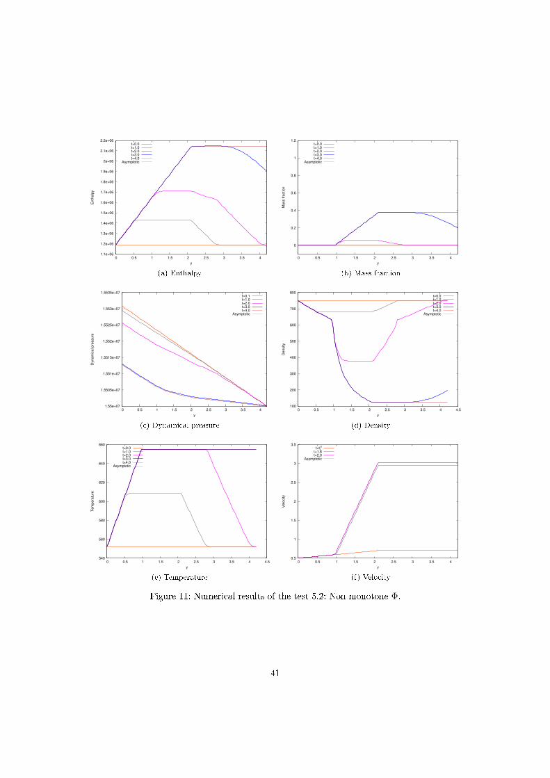
1.1e+06

1.2e+06

1.3e+06

1.4e+06

1.5e+06

1.6e+06

1.7e+06

1.8e+06

1.9e+06

2e+06

2.1e+06

2.2e+06

0 0.5 1 1.5 2 2.5 3 3.5 4

En

tha

lpy

y

t=0.0t=1.0t=2.0t=3.0t=4.0

Asymptotic

(a) Enthalpy

0

0.2

0.4

0.6

0.8

1

1.2

0 0.5 1 1.5 2 2.5 3 3.5 4

Ma

ss f

ractio

n

y

t=0.0t=1.0t=2.0t=3.0t=4.0

Asymptotic

(b) Mass fraction

1.55e+07

1.5505e+07

1.551e+07

1.5515e+07

1.552e+07

1.5525e+07

1.553e+07

1.5535e+07

0 0.5 1 1.5 2 2.5 3 3.5 4

Dyn

am

ica

l p

ressu

re

y

t=0.1t=1.0t=2.0t=3.0t=4.0

Asymptotic

(c) Dynamical pressure

100

200

300

400

500

600

700

800

0 0.5 1 1.5 2 2.5 3 3.5 4 4.5

De

nsity

y

t=0.0t=1.0t=2.0t=3.0t=4.0

Asymptotic

(d) Density

540

560

580

600

620

640

660

0 0.5 1 1.5 2 2.5 3 3.5 4 4.5

Te

mp

era

ture

y

t=0.0t=1.0t=2.0t=3.0t=4.0

Asymptotic

(e) Temperature

0.5

1

1.5

2

2.5

3

3.5

0 0.5 1 1.5 2 2.5 3 3.5 4

Ve

locity

y

t<tls

t=1.8t=2.0

Asymptotic

(f) Velocity

Figure 11: Numerical results of the test 5.2: Non monotone Φ.

41

tt1 t2 t3

Φ

Φ0

7%Φ0

(a) Φ(t)

tt1 t2 t3

ve

10v

0.2v

(b) ve(t)

Figure 12: Power density and entrance velocity for the test 5.3: A simpli�ed scenario for a Lossof Flow Accident.

1, 2 and 3. To simulate this scenario, the domain is �lled at �rst with liquid water and wehave a normal behaviour of the reactor: the pumps work normally and control rods are in upperposition. We impose at the entrance the velocity ve = 10v and the power density is equal to Φ0.These constants are chosen so as to prevent the appearance of mixture. The asymptotic state isreached at t ' 0.8 s.

At time t1 = 1.5 s most of the pumps stop, so that the entrance velocity decreases. At time t2the security system makes control rods drop into the core decreasing abruptly the power density.However, there is still some residual power density (here set to 7%Φ0). This instant t2 ' 2.85 scorresponds to the reaction time (0.3 s) of the safety system (drop of the control rods) aftermixture appears (t ' 2.55 s) and is detected. At time t3 the security pumps are turned on, thusthe in�ow is re-established. We then compute the solution until the asymptotic state is reached.Functions ve(t) and Φ(t) can be modelled as follows (see Figure 12):

ve(t) =

10v, if 0 ≤ t < t1,

0.2v, if t1 ≤ t < t3,

10v, if t ≥ t3,Φ(t) =

{Φ0, if 0 ≤ t < t2,

7%Φ0, if t ≥ t2.

In Figure 13 we report the behaviour of the mass fraction and temperature computed at di�erentinstants. Thanks to our model we can predict the appearance of some steam in the core dependingof the value of t3:

Case A: for t3 = 40 s, the asymptotic state corresponding to Φ = 7%Φ0 and ve = 0.2v isestablished. In this case, due to the residual power density the �uid is completelyvaporized at the top of the domain during the transition (see for example Figure 13a attime t = 30 s) even though there are only liquid and mixture phases in the correspondingasymptotic state.

Case B: for t3 = 20 s, the pumps are re-started soon enough so that the appearance of puresteam is avoided.

Case C: for t3 = 4 s, even though the pumps are re-started almost instantaneously, some mixtureappears in a large part of the domain.

In all cases when the pumps are re-started, the �uid comes back to the liquid phase. As expected,the sooner the pumps are re-started, the safer the situation.

42

0

0.2

0.4

0.6

0.8

1

1.2

0 0.5 1 1.5 2 2.5 3 3.5 4

Ma

ss f

ractio

n

y

t=0.0t=1.5t=3.0

t=30.0t=40.0t=50.0

550

600

650

700

750

800

850

900

0 0.5 1 1.5 2 2.5 3 3.5 4 4.5

Te

mp

era

ture

y

t=0.0t=1.5t=3.0

t=30.0t=40.0t=50.0

(a) Case A

0

0.2

0.4

0.6

0.8

1

1.2

0 0.5 1 1.5 2 2.5 3 3.5 4

Ma

ss f

ractio

n

y

t=0.0t=1.5t=3.0

t=10.0t=20.0t=25.0

540

560

580

600

620

640

660

0 0.5 1 1.5 2 2.5 3 3.5 4 4.5

Te

mp

era

ture

y

t=0.0t=1.5t=3.0

t=10.0t=20.0t=25.0

(b) Case B

0

0.2

0.4

0.6

0.8

1

1.2

0 0.5 1 1.5 2 2.5 3 3.5 4

Ma

ss f

ractio

n

y

t=0.0t=1.5t=3.0t=4.0t=5.0

540

560

580

600

620

640

660

0 0.5 1 1.5 2 2.5 3 3.5 4 4.5

Te

mp

era

ture

y

t=0.0t=1.5t=3.0t=4.0t=5.0

(c) Case C

Figure 13: Numerical mass fraction (left) and temperature (right) of the test 5.3: A simpli�edscenario for a Loss of Flow Accident.

43

6. Conclusion & Perspectives

We proposed in this paper simulations of a low Mach number model � named Lmnc � for �uid�ows in nuclear reactor cores coupled to an adaptive sti�ened gas equation of state (EOS) whichvaries according to the phase of the coolant �uid (which can be pure liquid water, pure steamor mixture of these two phases). The monodimensional (1D) numerical strategy we worked outleads to accurate and relevant qualitative results in accordance with what was expected. Theseresults were obtained with an optimal computational cost since the velocity and the dynamicpressure are directly integrated in the 1D case.

More precisely, compared to a previous study [6], the present work enables to deal with more re-alistic situations insofar as the model allows for phase transition and, thus, for accidental scenariisuch as a Loss of Flow Accident (LOFA) induced by a coolant pump trip event. Nevertheless, themethod used to determine parameters involved in the sti�ened gas EOS seems to be restrictivegiven the range of temperature that must be considered. That is why another strategy will beinvestigated in [18] using tabulated laws instead of the sti�ened gas EOS.

From a numerical point of view, a variant of the classic method of characteristics was proposed.It relies on the EOS and provided second-order accurate results. This algorithm was comparedto the unsteady analytical solutions derived in this study for di�erent data sets including con�g-urations where phase transition occurs.

Moreover, we recall that the thermodynamic pressure is constant in the Lmnc model. Hence,whatever the EOS used to model each phase and no matter what the dimension of the domain(1D, 2D or 3D), the computational cost related to the EOS will be much lower in the discretizationof the Lmnc model than in any strategy for the compressible model.

The adaptation of the proposed algorithm to dimensions 2 and 3 will be carried out in futureworks. However, it must be underlined that although the Lmnc model may be a useful toolfor safety studies, it is not designed to handle all potential situations especially when the Machnumber cannot be considered small anymore. This is why it is important to study the possibilityto couple the Lmnc model to the compressible system from which it is derived (this approachwill be investigated in future works). Likewise, couplings with systems dedicated to other circuitsin the reactor must be considered.

A. Derivation of the mixture density formula

The mechanic and thermodynamic equilibria hypothesis in the mixture at saturation impliesthat the pressures are identical in each phase. This allows to obtain (2.2) by using (2.1b). Thisresults in the equality for the mixture density ρm

ρm =αρsgh

sg + (1− α)ρs`h

s`

h= αρsg + (1− α)ρs`

where ρsκ and hsκ are the density and the enthalpy of the phase κ ∈ {`, g} at saturation, i.e.ρsκ = ρκ

(p, T s(p)

)and hsκ = hκ

(p, T s(p)

)where T s(p) is the temperature T solution of g`(p, T ) =

gg(p, T )). We deduce α is prescribed by

α(h, p) = ρs`h− hs`

(ρsghsg − ρs`hs`)− h · (ρsg − ρs`)

.

44

Hence we obtain

ρm(h, p) = ρs` + α(h, p) · (ρsg − ρs`) =ρsgρ

s`(h

sg − hs`)

ρsghsg − ρs`hs` − h · (ρsg − ρs`)

,

which gives the expression (2.3) of ρm as a function of (h, p).

B. Computation of the speed of sound for two-phase media

We detail in this section how to express the speed of sound in the diphasic case. This enables inparticular to compute the Mach number in any case and to highlight that it remains small.

B.1. General case

In [3, 22, 23], it has been proved that the speed of sound of the mixture is always positive. Tocompute explicitly the speed of sound as a function of the enthalpy and the pressure, we startfrom the usual thermodynamic relation

Tdη = dε− p

ρ2dρ.

On the one hand, the relation h = ε+ pρ coupled to the previous statement leads to

d(ρε) = (ρT )dη + hdρ.

On the other hand, we have

d(ρε) =∂(ρε)

∂ρ

∣∣∣∣p

dρ+∂(ρε)

∂p

∣∣∣∣ρ

dp.

Therefore, the comparison of the two previous equalities yields

dp =h− ∂(ρε)

∂ρ

∣∣∣p

∂(ρε)∂p

∣∣∣ρ

dρ+ρT

∂(ρε)∂p

∣∣∣ρ

dη,

so that the speed of sound c is given by

c2 def=∂p

∂ρ

∣∣∣∣η

=h− ∂(ρε)

∂ρ

∣∣∣p

∂(ρε)∂p

∣∣∣ρ

=h− ∂(ρh)

∂ρ

∣∣∣p

∂(ρh)∂p

∣∣∣ρ− 1

, (B.1)

since ρε = ρh− p.

� In the pure phase κ ∈ {`, g}, the volume fraction α is 0 (i.e. κ = `) or 1 (i.e. κ = g), sothat ρ = ρκ, h = hκ and equation (B.1) becomes

c2κ =−ρκ ∂hκ

∂ρκ

∣∣∣p

ρκ∂hκ∂p

∣∣∣ρκ− 1

. (B.2a)

45

� In the mixture, using (2.2) and noticing that ρκhκ = ρsκhsκ (since T = T s(p) in the mixture),

which only depends on p, we can write

∂(ρh)

∂ρ

∣∣∣∣p

=∂α

∂ρ

∣∣∣∣p

(ρsghsg) + α

�����∂(ρsghsg)

∂ρ

∣∣∣∣p

− ∂α

∂ρ

∣∣∣∣p

(ρs`hs`) + (1− α)

�����∂(ρs`hs`)

∂ρ

∣∣∣∣p

,

∂(ρh)

∂p

∣∣∣∣ρ

=∂α

∂p

∣∣∣∣ρ

(ρsghsg) + α

∂(ρsghsg)

∂p

∣∣∣∣ρ

− ∂α

∂p

∣∣∣∣ρ

(ρs`hs`) + (1− α)

∂(ρs`hs`)

∂p

∣∣∣∣ρ

.

Because of (2.1a), we compute the partial derivatives of the volume fraction α

∂α

∂ρ

∣∣∣∣p

=1

ρsg − ρs`,

∂α

∂p

∣∣∣∣ρ

=−(ρs`)

′(ρsg − ρs`)− (ρ− ρs`)((ρsg)′ − (ρs`)′)

(ρsg − ρs`)2= −

α(ρsg)′ + (1− α)(ρs`)

′

ρsg − ρs`,

where (ρsκ)′ is the derivative of p 7→ ρsκ(p). Hence

(cm(h, p)

)2 def=h− ρsgh

sg−ρ

s`hs`

ρsg−ρs`

−[α(ρsg)′ + (1− α)(ρs`)

′]ρsgh

sg−ρs`h

s`

ρsg−ρs`+ α(ρsgh

sg)′ + (1− α)(ρs`h

s`)′ − 1

, (B.2b)

where (ρsκhsκ)′ denotes the derivative of the product p 7→ ρsκ(p)hsκ(p).

Finally, the speed of sound is given by

c(h, p) =

c`(h, p), if h ≤ hs`(p),

cm(h, p), if hs`(p) < h < hsg(p),

cg(h, p), if h ≥ hsg(p).

(B.3)

Remark B.1. The speed of sound is discontinuous across the saturation curve, and it is smallerin the mixture than in any pure phase. The minimum value is reached for void ratios close tozero (see [22] and Figure 3d).

B.2. Sti�ened gas EOS

To compute the speed of sound cκ in a pure phase (κ ∈ {`, g}) using (B.2a), we need to expressthe enthalpy h as a function of the density ρκ and the pressure p. Inverting (2.12a), we obtain

hκ(ρ, p) = qκ +γκ(p+ πκ)

ρ(γκ − 1)

so that (B.2a) becomes

cκ(ρ, p) =

√γκ(p+ πκ)

ρ.

In the mixture, the speed of sound cm satis�es equation (B.2b) which is written as(cm(h, p)

)2=

h− qm−[α(ρsg)

′ + (1− α)(ρs`)′]qm + α(ρsgh

sg)′ + (1− α)(ρs`h

s`)′ − 1

.

46

In this expression, we introduced the following notations

(ρsκ)′(p) =1

(γκ − 1)cvκTs(p)

(1− (p+ πκ)

(T s)′

T s(p)

),

(ρsκhsκ)′(p) =

1

(γκ − 1)cvκTs(p)

(qκ + γκcvκT

s(p)− (p+ πκ)qκ(T s)′

T s(p)

),

(T s)′(p) =

(γg − 1)cvgp+ πg

− (γ` − 1)cv`p+ π`

(cvgγg − cv`γ`) +qg − q`T s(p)

T s(p) =

1

ρsg(p)− 1

ρs`(p)

hsg(p)− hs`(p)T s(p) =

T s(p)

pβm(p).

C. Approximation of the water EOS with the sti�ened gas

law

In this appendix, we describe the method introduced in [31,32,40] to choose parameters describingeach pure phase of water with a sti�ened gas law to best �t with saturated curves (see Figure 2a).Then, we determine relevant values for liquid water and steam.

More precisely, we suppose that each phase is described by its own sti�ened gas EOS (2.7), sothat we have to compute �ve constants for each phase: the speci�c heat at constant volume cvκ ,the adiabatic coe�cient γκ, the reference pressure πκ, the binding energy qκ and the referenceentropy q′κ de�ned by (2.9). We recall that κ = ` refers to the liquid phase and κ = g to thevapor one. These parameters will be determined using experimental values at saturation.

The sti�ened gas law consists of the following expressions for the density, the enthalpy and theGibbs potential as functions of the temperature T and the pressure p:

ρκ(T, p) =p+ πκ

(γκ − 1)cvκT, (C.1a)

hκ(T, p) = qκ + γκcvκT, (independent of p) (C.1b)

gκ(T, p) = qκ + T[cvκγκ − q′κ − cvκγκ lnT + cvκ(γκ − 1) ln(p+ πκ)

]. (C.1c)

For a given temperature T , the experimental data needed for the computation are the pres-sure at saturation psexp(T ), the enthalpies at saturation hsκ,exp(T ) and the densities at saturationρsκ,exp(T ). We can �nd these data in [33] for several �uids. Let T0 and T1 two reference temper-atures (recorded in [33]) between the triple point and the critical point (see Figure 2b).

• Step I: computation of γκcvκ . From the analytical expression of the enthalpy (C.1b), wehave h′κ(T ) = γκcvκ . This yields an averaged value of the product cpκ

def= γκcvκ by means ofa linear approximation of the experimental enthalpies between reference states T0 and T1

as

cpκ =hsκ,exp(T1)− hsκ,exp(T0)

T1 − T0. (C.2)

47

• Step II: computation of qκ. Equation (C.1b) applied to the reference state T0 provides theapproximation of the binding energy qκ:

qκ = hsκ,exp(T0)− cpκT0.

• Step III: computation of πκ. At saturation, there is an algebraic relation between the tem-perature and the pressure, e.g. we can write p = ps(T ). Thus, using (C.1a), the speci�cdensities at saturation are expressed as

ρsκ(T ) = ρκ(T, ps(T )

)=

ps(T ) + πκ(cpκ − cvκ)T

, (C.3)

which evaluated at T0 and T1 yields

ρsκ(T1)

ρsκ(T0)=

(ps(T1) + πκ)T0

(ps(T0) + πκ)T1,

so that we can determine an averaged value of the coe�cient πκ using experimental valuesof the density and the pressure at saturation

πκ =T0ρ

sκ,exp(T0)psexp(T1)− T1ρ

sκ,exp(T1)psexp(T0)

T1ρsκ,exp(T1)− T0ρsκ,exp(T0).

• Step IV: computation of cvκ . Equation (C.3) applied to the reference state T0 providesthe approximation of cvκ

cvκ = cpκ −psexp(T0) + πκ

T0ρsκ,exp(T0).

• Step V: computation of γκ. Using (C.2) we deduce the approximation of γκ

γκ =cpκcvκ

.

• Step VI: computation of q′κ. At thermodynamic equilibrium, the two Gibbs potentials areequal. Using (C.1c), this implies

A ln(ps(T ) + πg

)−B ln

(ps(T ) + π`

)− C(lnT − 1) +

D

T+ q′` − q′g = 0

with

A def= cpg − cvg , B def= cp` − cv` , C def= cpg − cp` , D def= qg − q`.

By convention, we take q′` = 0 J ·K−1 and determine the coe�cient q′g using experimentalvalues of the pressure at saturation

q′g = A ln(psexp(T0) + πg

)−B ln

(psexp(T0) + π`

)− C(lnT0 − 1) +

D

T0.

48

Phase cv [J ·K−1] γ π [Pa] q [J · kg−1] q′ [J ·K−1]Liquid 1816.2 2.35 109 −1167.056×103 0Vapor 1040.14 1.43 0 2030.255×103 −23310

Table 1: Liquid water and steam, parameters computed in [31,32].

Reference states T0 and T1 must now be speci�ed. First, T0 is a reference state chosen in orderto have the best �t between the theoretical pressure ps(T ) and the experimental one psexp(T ).Secondly, this strategy for the determination of parameters for a sti�ened gas EOS is accurateif the two reference states are su�ciently close. Practically (following [31, 32]), we took for theliquid phase T0 = 298 K and T1 = 473 K (steps I and II) and T0 = 439 K and T1 = 588 K (stepsIII to VI). As for the steam, we set T0 = 298 K and T1 = 473 K in any step.

The values for liquid water and steam are given in Table 1. As underlined in [22, 31, 32], theseparameter values yield reasonable approximations over a temperature range from 298 K to 473 K.Nevertheless near the critical point, there are some restrictions due to the nonlinearity of theenthalpy with respect to the temperature. To circumvent this limitation, we shall propose in [18] anew strategy to better approximate the thermodynamic quantities involved in the Lmncmodel.

References

[1] TRACE V5.0 Theory Manual, Field Equations, Solution Methods and Physical Models.Technical report, U.S. Nuclear Regulatory Commission, 2008.

[2] A. Acrivos. Method of characteristics technique. Application to heat and mass transferproblems. Ind. Eng. Chem., 48(4):703�710, 1956.

[3] G. Allaire, G. Faccanoni, and S. Kokh. A strictly hyperbolic equilibrium phase transitionmodel. C. R. Acad. Sci. Paris Ser. I, 344:135�140, 2007.

[4] A.S. Almgren, J.B. Bell, C.A. Rendleman, and M. Zingale. Low Mach number modeling oftype Ia supernovae. I. hydrodynamics. Astrophys. J., 637(2):922, 2006.

[5] A.S. Almgren, J.B. Bell, C.A. Rendleman, and M. Zingale. Low Mach number modeling oftype Ia supernovae. II. energy evolution. Astrophys. J., 649(2):927, 2006.

[6] M. Bernard, S. Dellacherie, G. Faccanoni, B. Grec, O. La�tte, T.-T. Nguyen, and Y. Penel.Study of low Mach nuclear core model for single-phase �ow. ESAIM Proc., 38:118�134,2012.

[7] D. Bestion. The physical closure laws in the CATHARE code. Nucl. Eng. Des., 124(3):229�245, 1990.

[8] H. B. Callen. Thermodynamics and an Introduction to Thermostatistics. John Wiley &sons, second edition, 1985.

[9] V. Casulli and D. Greenspan. Pressure method for the numerical solution of transient,compressible �uid �ows. Internat. J. Numer. Methods Fluids, 4(11):1001�1012, 1984.

[10] S. Clerc. Numerical Simulation of the Homogeneous Equilibrium Model for Two-PhaseFlows. J. Comput. Phys., 181(2):577�616, 2002.

49

[11] P. Colella and K. Pao. A projection method for low speed �ows. J. Comput. Phys.,149(2):245�269, 1999.

[12] J.M. Delhaye. Thermohydraulique des réacteurs. EDP sciences, 2008.

[13] S. Dellacherie. On a diphasic low Mach number system. ESAIM Math. Model. Numer.Anal., 39(3):487�514, 2005.

[14] S. Dellacherie. Numerical resolution of a potential diphasic low Mach number system. J.Comput. Phys., 223(1):151�187, 2007.

[15] S. Dellacherie. Analysis of Godunov type schemes applied to the compressible Euler systemat low Mach number. J. Comput. Phys., 229(4):978�1016, 2010.

[16] S. Dellacherie. On a low Mach nuclear core model. ESAIM Proc., 35:79�106, 2012.

[17] S. Dellacherie, G. Faccanoni, B. Grec, F. Lagoutière, E. Nayir, and Y. Penel. 2D numericalsimulation of a low Mach nuclear core model with sti�ened gas using Freefem++. ESAIM.Proc., (accepted).

[18] S. Dellacherie, G. Faccanoni, B. Grec, and Y. Penel. Study of low Mach nuclear core modelfor two-phase �ows with phase transition II: tabulated EOS. In preparation.

[19] M. Drouin, O. Grégoire, and O. Simonin. A consistent methodology for the derivation andcalibration of a macroscopic turbulence model for �ows in porous media. Int. J. Heat MassTran., 63(0):401 � 413, 2013.

[20] D. R. Durran. Numerical methods for �uid dynamics, volume 32 of Texts in Applied Math-ematics. Springer, New York, second edition, 2010. With applications to Geophysics.

[21] P. Embid. Well-posedness of the nonlinear equations for zero Mach number combustion.Comm. Partial Di�erential Equations, 12(11):1227�1283, 1987.

[22] G. Faccanoni. Étude d'un modèle �n de changement de phase liquide-vapeur. Contributionà l'étude de la crise d'ébullition. PhD thesis, École Polytechnique, France, November 2008.

[23] G. Faccanoni, S. Kokh, and G. Allaire. Modelling and simulation of liquid-vapor phasetransition in compressible �ows based on thermodynamical equilibrium. ESAIM Math.Model. Numer. Anal., 46:1029�1054, September 2012.

[24] P. Fillion, A. Chanoine, S. Dellacherie, and A. Kumbaro. FLICA-OVAP: A new platformfor core thermal�hydraulic studies. Nucl. Eng. Des., 241(11):4348�4358, 2011.

[25] E. Goncalvès and R. F. Patella. Numerical study of cavitating �ows with thermodynamice�ect. Comput. & Fluids, 39(1):99�113, 2010.

[26] J.M. Gonzalez-Santalo and R.T. Jr Lahey. An exact solution for �ow transients in two-phasesystems by the method of characteristics. J. Heat Transf., 95(4):470�476, 1973.

[27] W. Greiner, L. Neise, and H. Stöcker. Thermodynamics and statistical mechanics. Springer,1997.

[28] H. Guillard and C. Viozat. On the behaviour of upwind schemes in the low Mach numberlimit. Comput. & Fluids, 28(1):63�86, 1999.

[29] S. Jaouen. Étude mathématique et numérique de stabilité pour des modeles hydrodynamiquesavec transition de phase. PhD thesis, Université Paris 6, 2001.

50

[30] M.F. Lai, J.B. Bell, and P. Colella. A projection method for combustion in the zero Machnumber limit. In Proc. 11th AIAA Comput. Fluid Dyn. Conf., pages 776�783, 1993.

[31] O. Le Métayer, J. Massoni, and R. Saurel. Elaborating equations of state of a liquid and itsvapor for two-phase �ow models. Int. J. Therm. Sci., 43(3):265�276, 2004.

[32] O. Le Métayer, J. Massoni, and R. Saurel. Modelling evaporation fronts with reactiveRiemann solvers. J. Comput. Phys., 205:567�610, 2005.

[33] E. W. Lemmon, M. O. McLinden, and D. G. Friend. Thermophysical Properties of FluidSystems. National Institute of Standards and Technology, Gaithersburg MD, 20899.

[34] A. Majda and K.G. Lamb. Simpli�ed equations for low Mach number combustion with strongheat release, volume 35 of IMA Vol. Math. Appl. Springer-Verlag, 1991. Dynamical issuesin combustion theory.

[35] A. Majda and J. Sethian. The derivation and numerical solution of the equations for zeroMach number combustion. Combust. Sci. Technol., 42(3-4):185�205, 1985.

[36] R. Meniko� and B.J. Plohr. The Riemann problem for �uid �ow of real materials. Rev.Modern Phys., 61(1):75�130, 1989.

[37] S. Müller and A. Voss. The Riemann problem for the Euler equations with nonconvexand nonsmooth equation of state: construction of wave curves. SIAM J. Sci. Comput.,28(2):651�681 (electronic), 2006.

[38] Y. Penel. An explicit stable numerical scheme for the 1D transport equation. DiscreteContin. Dyn. Syst. Ser. S, 5(3):641�656, 2012.

[39] Y. Penel. Existence of global solutions to the 1D abstract bubble vibration model. Di�entialIntegral Equations, 26(1-2):59�80, 2013.

[40] R. Saurel, F. Petitpas, and R. Abgrall. Modelling phase transition in metastable liquids:application to cavitating and �ashing �ows. J. Fluid Mech., 607:313�350, 2008.

[41] G.I. Sivashinsky. Hydrodynamic theory of �ame propagation in an enclosed volume. ActaAstronaut., 6:631�645, 1979.

[42] G. Volpe. Performance of compressible �ow codes at low Mach numbers. AIAA J., 31(1):49�56, 1993.

[43] A. Voss. Exact Riemann solution for the Euler equations with nonconvex and nonsmoothequation of state. PhD thesis, RWTH Aachen, 2005.

[44] N. Zuber. Flow excursions and oscillations in boiling, two-phase �ow systems with heataddition. In Symposium on Two-phase Flow Dynamics, Eindhoven EUR4288e, pages 1071�1089, 1967.

51