eries 01 Aerodynamics 04

Experimental and Computational Study of a Blunt Cylinder-Flare Model in High Supersonic Flow

E.M. Houtman/WJ. Bannink/B.H. Timmerman

Delft University Press

Experimental and Computational Study of a Blunt Cylinder-Flare Model in High Supersonic Flow

8ibliotheek TU Delft

1111111111111 C 3021881

2392 344 9

•• U1 Li .... Ma. 11. i Ij» i i i i I I t I I I i i i IIIIMn _lilA'. , i_Nili 111 'Je . IJ ' , i j

Series 01: Aerodynamics 04

Experimental and Computational Study of a Blunt Cylinder-Flare Model in High Supersonic Flow

E.M. Houtman/W.J. Bannink/B.H. Timmerman

Delft University Pre ss / 1998

Published and distributed by:

Delft University Press Mekelweg 4 2628 CD Delft The Netherlands Telephone +31 (0)152783254 Fax +31 (0)152781661 e-mail: DUP@DUP.TUDelft.NL

by order of:

Faculty of Aerospace Engineering Delft University of Technology Kluyverweg 1 P.O. Box 5058 2600 GB Delft The Netherlands Telephone +31 (0)152781455 Fax +31 (0)15278 1822 e-mail: Secretariaat@LR.TUDelft.NL website: http://www.lr.tudelft.nl/

Cover: Aerospace Design Studio, 66.5 x 45.5 cm, by: Fer Hakkaart, Dullenbakkersteeg 3, 2312 HP Leiden, The Netherlands Tel. + 31 (0)71 512 67 25

90-407-1567-X

Copyright © 1 998 by Faculty of Aerospace Engineering

All rights reserved . No part of the material protected by this copyright notice may be reproduced or utilized in any form or by any means, electron ic or mechanical, including photocopying, recording or by any information storage and retrieval system, without written permission from the publisher: Delft University Press.

Printed in The Netherlands

CONTENTS

LIST OF SYMBOLS iv

1 INTRODUCTION 1

2 EXPERIMENTS 2 2.1 Experimental equipment and conventional techniques 2 2.2 Digital Holographic InteIferometry 3

3 NUMERICAL FLOW SIMULATIONS 8 3.1 Discretization of the Euler equations . 8 3.2 Solution procedure . JO 3.3 Computational grid. . . . . . . 11 3.4 Numerical simulation of InteIferometry 12

4 RESULTS 13 4.1 Visualization studies 13 4.2 InteIferometry 18 4.3 Computations 23 4.4 SuIface pressure distributions 26

5 CONCLUSIONS 31

REFERENCES 32

Acknowledgements

The authors wish to express their gratitude to the folJowing students who contributed to this inves­tigation: Mr: P.A. Lusse who perforrned the visualization tests, Mr. S. Reginato who perforrned the surface pressure measurements and Mr. C. Beets who perforrned the grid generation and preliminary computations. The technical staff of the High Speed Laboratory is acknowledged for its technical assistance throughout the experimental part of this project.

LIST OF SYMBOLS

General

bold BOLD

Arabic

C

Cp, Ct"

e

et Lg,h f SFF

F H ht I i.j, k K L -'1 ,'v/np

S"S)'Sk Sf n

P Pt q

R

rijk r m

S 6.S 8

T

lt, r, lC

F 6.\/

vectors of variables are indicated in bold lowercase matrices are indicated in BOLD capitals

lift coefficient drag coefficient speed of sound specific heats at constant pressure and constant volume respectively intemal energy total energy per unit of mass flux vectors in x. y . .:-direction respectively numerical flux function spatial discretization of goveming equations Jacobian of discretized system total enthalpy identity matrix indices in computational space Gladstone-Dale constant width of test-section Mach number Mach number based on the velocity component in the direction of the local pressure gradient number of volumes in i , j, k direction respectively number of faces of control volume unit normal vector statie pressure total pressure velocity vector gas constant limiter function applied to i-direction

source term boundary of control volume surface of cell face coordinate along light ray rotation matrix time velocity components in x . y.::: directions respectively control volume cell volume

X. y,z i .y.z

Greek

Q

J1 À

ç p

Pint

o [li jk

a[l

Subscripts

Cartesian coordinate system rotated Cartesian coordinate system

angle of attack ratio of specific heats (cp / Ct = 1.4) difference operator forward and backward differences in i-direction flow deflection angle constant in higher order interpolation function Mach angle wavelength of light source parametric coordinate density integrated density along light path phase angle control volume cell face of control volume

ARS Approximate Riemann Sol ver at' averaged quantity dis t, undist flow field with and without model i,j. k grid point indices m cell face index max SFF X.y.z 0C

maximal Numerical Flux Function components in x. y. z direction free-stream condition

Chapter 1

INTRODUCTION

The present investigation of high-supersonic and hypersonic f10w s around (blunt) bodies at large an­gle of attack has been initiated by the development of re-entry spacecraft (Space Shuttle, Hermes) and advanced launchers. In general the flow at these conditions is characterized by several phenom­en a, such as the presence of a bow shock, embedded shocks, regions of separated and vortical flow, shock-boundary layer and shock-shock interactions and high heating rates near discontinuities at the model surface, such as cockpit-body and wing-body junctions. The prediction of the complex three­dimensional flow field provides achallenging task for numeri cal methods. In order to validate such computer codes, experimental data of good quality are a prerequisi te. For validation of the codes it is satisfactory to study simple configurations, with which interesting flow phenomena can be generated.

Realistic hypersonic flow conditions during re-entry are difficult to simulate in a wind tunnel and require special facilities. Many flow phenomena, such as separation and vortex formation, shock­boundary layer interactions and shock-shock interactions, already appear at high supersonic Mach numbers (3-4). These flow conditions can be realized in standard facilities , for which a variety of measuring techniques is available. In view of these considerations an experimental program on a sim­ple test configuration has been staned at the High Speed Aerodynamics Laboratory of the Faculty of Aerospace Engineering. Several wind tunnel tests have been performed on a hemispherical-nose­cylinder with a 30° conical afterbody. Although a simple geometry was selected, several interesting flow phenomena were observed. The leeward flow field at medium to high angle of attack is domi­nated by large separated regions, vortical flow and embedded shocks. The windward flow field is less compJicated, but at large angles of attack an interesting shock-shock interaction exists, which influ­ences the surface flow. The model has been investigated in the high-supersonic flow regime (Mach number 3 up to 4) and angles of attack up to 20c

. Under these flow conditions the assumption of a perfect gas is still valid. The purpose of this investigation was to provide aerodynamic data of good quality and high resolution in order to validate computer codes.

Besides the experimental program, a number of numerical simulations wi th a three-dimensional Euler code have been performed. Within th is investigation, emphasis was put on the simulation of inviscid flow phenomena, like the capturing of the bow shock and the flare shock and their interaction at high angles of attack.

The work described in this report has been sponsored by the European Space Research and Technology Centre (ESTEC, Noordwijk, the Netherlands) under Purchase Order number 141125 (date: 28-03-1994). The study was monitored by 1. Muylaert, Aerothermodynamics section (YPA) of ESTEC.

Chapter 2

EXPERIMENTS

2.1 Experimental equipment and conventional techniques

The major part of the experiments are performed in the TST-27 wind tunnel of the High Speed Aero­dynamics Laboratory. This is a blow-down wind tunnel with a test-section of 2i x 28 cm2 (height x width), which can be operated in the Mach number range Moe = 0.5 - 4. Interferometric exper­iments are performed in the ST-I5 supersonic blow-down wind tunnel. which has a test-section of 1.5 x 15 cm2 . This wind tunnel is equipped with a fixed nozzle, generating a Mach number of 2.9.5 in the test-section.

The model is axi-symmetric, consisting of a cylinder with a hemispherical head. a conical flare with an angle of 30° and a cylindrical tail. The coordinate system used and the dimensions of the model are given in Fig. 2.1: the dimensions of the model used in the smaller ST-15 wind tunnel are given between brackets. For the tests in the TST-27 wind tunnel two models were made. Asolid black-

Sidevicw Fromview

z A ~=15(7) x -------- ----- _ . . -

:'-. 60(28) ~

99 (46.2) ., 75 (35) I' ~~-.

127 (59.5) dimensions in mm (mterferometry)

Figure 2.1: Geometry of test configuration

painted model was used for several experiments, including: qualitative flow visualization as obtained from shadowgraph- and Schlieren techniques, surface oil-flow visualizations and flow field explo­rations with a five-hole probe (Lusse 1992). Another model was used for measuring the surface pres­sure distribution (Reginato 1993). This model was equipped with 75 pressure orifices, located at three generators with a 10° spacing (Fig. 2.2). At the rear of the model screw holes all ow roll angles with a :360° range and a 5° stepsize, which enables the determination of a pressure distribution over the en­tire model with a high resolution. The location of pressure orifices is concentrated in regions where a complex (separated) flow was expected, i.e. the region where the hemispherical head changes into the cylindrical part and the region near the conical wedge.

The tests are performed at Mach numbers i\lIoe of :3,3 .. 5 and 4, and angles of attack Ct from 0° to 20°. The Reynolds number based on a model-length of 12i mm ranges from 6 x 106 to i.6 X 106 . Part ofthe results (surface pressures and shadowgraph pictures) is available on demand for validation purposes.

2

iN" Wiiifiih' 1'11 '11 hAiNitibiilii " ie "iW .; _; ri ij Wi 4 i p i ia' Rtt "iI. 11 i.' h ft

:: f!sel 0 39

Figure 2.2: Location of pressure orifices on test configuration

2.2 Digital Holographic Interferometry

Oigital Holographic Interferometry (DHI) is applied to obtain quantitative information about the den­sity distribution in the flow field. In the dual-reference-beam, plane-wave OHI set-up used here, holographic interferometry for recording of a flow field in an interferogram is combined with phase­stepping ofthis interferogram and digital image-processing to compute the phase map from these digi­tised interferograms (Lanen et al. 1992; Lanen 1992). This phase map represents the deformation of the wavefront of the light beam which has traversed the flow field and from it the mean density in the flow field can be calculated. As the results only contain the density integrated along the light paths, quantitative interpretation for 3-0 f10ws is not as direct as in the case of 2-0 flows . Main advantage of this optical technique is that a large part of the flow field can be measured at one instant with a high resolution of data and without disturbance of the flow.

The flow field was recorded with the plane-wave holographic interferometer set-up shown in Fig. 2.3. A ruby pulse laser was used to expose the holographic plate, thereby freezing the flow-field image. The pulse length used here is 0 .. ) msec, resulting in a limited sensitivity to unsteady flow phenomena. In the post-processing ph ase the plate is illuminated with a (continuous) CW HeNe laser and four phase-stepped interferograms are generated. which are digitally stored and processed. From these four interferograms a 2-0 ph ase image (512 x 512 pixels, representing a region of ï5 x ï.) mm2 in the flow) is obtained, which contains information about the flow-field density averaged over the light path (tunnel width). The use of two reference paths makes it possible to store two different flow situations on the same holographic plate in such a way that they can be reconstructed separately.

The interferometer set-up is placed over the test section of the wind tunnel. Optical access is provided

3

'"

Rl PBSC R2

PULSED RUBY LASER CW HeNe lASER

~ ,,~~~~------------------------~~-

M4/''--+--,-ii'' "3 ';

TEST secnoN

"5 W1 W2

Figure 2.3: Two-reference-beam, plane-wave holographic interferometer. BSP: 50/50 beamsplit­ter plate; H: holographic plate; L l '" . L.J. L6: positive lens, L4 ' Ls: negative lens; MI ..... ::'1'14 : 45° -incidence HEL-mirror; :\1.s. :\1,. :\18 : mirror: M6 : 0° -incidence HEL-mirror; PBSC: polarising beamsplitting cube; PZT: piezo-electric transducer: R l . .... R 3: ~.\-retardation plate; S: mechanical shutter; H 'l · Vl'z: test-section window; SF: spatial filter

by (circular) windows in the tunnel side walls. The main flow direction is norm al to the plane of drawing. The model is placed in the middle of the test section. In the reconstruction stage the CCD­camera is focussed at the symmetry plane of the flow, as for axi-symmetric flows this has been shown to minimise refraction problems (Montgomery and Reuss 1982). Hence, the inverse Abel transform can be used to compute the radial refractive index distribution from the interferometric data while neglecting refractive distortion.

The wind tunnel is started with the model in the field of view. With mirror ~18 unblocked the ruby laser is fired once to record the "model flow". Subsequently a recording of the "undisturbed flow" is made, af ter having retracted the model, out of the field of view (Fig. 2.4), firing the laser for the second time with Ms blocked and M, unblocked. During the reconstruction phase, the object beam is blocked, while both reference beams are recreated by unblocking Mi as weil as 1"18' The plane-wave interferogram resulting from those two reconstructions can be subjected to phase-stepping by trans­lating mirror M" thus enabling an accurate automatic digital computation of the phase shift (Lanen et al. 1992). The method measures the deformation of the wavefront of a (laser) light beam caused by spatial density gradients in the flow field.

Quantitative deduction of the wave front distortion from interferograms requires application of the phase stepping technique to generate at least three phase-stepped interferograms and the application of digital image processing routines to compute the wave front deformation from these digitized inter­ferograms. This procedure overcomes certain ambiguity problems. usually occuring when the evalu­ation is based on the principle of fringe counting.

In the phase map modulo 2" resulting from ph ase stepping this "flow" hologram, horizontal background fringes can be seen (Fig. 2.5.a). These result from the difference between the wave­length at which the hologram is recorded (.\r uby =693.4 nm) and that at which it is reconstructed (.\HeNe =632.8 nm). These background fringes can be removed in two ways. The first one makes use of the fact that the fringe-effect caused by a difference in recording and reconstruction wavelength

4

I' Ir

lAewing Pvea - -~

-' . ..

Figure 2.4: Streamwise translation of model bet ween successive exposures of holographic plate

(a) Superimposed Iinear phase distribution. obtained

fro m "flow" hologram (b) Reference fringes . obtained from reference holo­

gram

Figure 2.5: Phase maps modulo 2" radians

5

is similar to that which occurs when the direction of the reconstruction beam differs from that in the recording stage (Françon 1974). Therefore, the background fringes can be eliminated by slightly

rotating mirror Ms, thereby producing an infinite fringe pattem. Phase-stepping and image processing this interference pattem then directly gives the phase modulo 2". The second solution avoids chang­ing anything to the set-up, by recording an additional hologram of which the reconstructed fringe pattem will only contain the background fringes. This reference hologram is made by two exposures in a no flow situation. By subtracting the phase maps of the reference hologram (Fig. 2.5.b) from the flow hologram, the real phase map modulo 2" is obtained. This second method was used to obtain the results presented in this report.

Figure 2.6: Phase map modulo 27i showing steady deviations from uniform supersonic flow

The phase map (Lanen 1992), which represents the deformation of the wave front of the light beam traversing the flow field (scene beam), may be written as an integral of the refractive index n along the light rays:

2n(J J ) .6.d>( x , z ) = T . ndistds - . n ,.mdistds

ut undtSt

(2.1 )

Here ~Q denotes the phase difference between the undisturbed scene beam and the disturbed scene beam, À the wavelength of the pulsed laser, n dist the refractive index in the disturbed flow field (flow with model) and nundist the refractive index in the undisturbed flow field (flow without model) . The coordinate s is measured along the light rays and (x. :;) represents the projection plane. The refractive index n is linearly coup led to the density p via the relation :

n = 1 + K p (2.2)

in which K is the Gladstone-Dale constant, which is a characteristic for the gas through which the light passes. Using this relation, the phase map can be written as a function of the density p(x. y.:;)

6

in the flow field :

(2.3)

so that the integrated density Pint along the light path may be determined from the phase angle:

! L

1 /2 1 ). ~Q Pint = L p(X, y, z) ds = Poe + L A' 2" (2.4)

- ~ L

To assess the quality of the free stream in the wind tunnel, Fig. 2.6 shows the phase map obtained by comparing the undisturbed flow to the no flow situation. It shows an average phase gradient in the flow direction of about one wavelength over ï5 mmo which corresponds to a variation in density of 0.02 kg/ m3 (i.e. 3% of the average Poe , corresponding to 1 % change in :\1",,) . This agrees with earl ier pressure probe measurements (Bannink 1963) which showed a decrease in Mach number of OA / m in the flow direction. Also, disturbance lines can be seen running at the Mach angle ( /l x = 22°) .

7

- --~ -~--------------------

Chapter 3

NUMERI CAL FLOW SIMULATIONS

3.1 Discretization of the Euler equations

Numerical simulations were performed using a code based on a cell-centred fini te-volume discretiza­tion of the three-dimensional Euler equations. The Euler equations, expressing conservation of mass, momentum and energy for a compressible perfect gas, will be formulated in conservative form . In a Cartesian coordinate system the Euler equations in a conservative differential form are given by:

where q is the vector of the conserved variables:

q = (p,pu.pv . pu"pet )T

and f ( q) , g( q ) and h( q) are the flux vectors , given by:

f (q) (pu , pu 2 + p , puv , puw , puht ) T

g (q)

h (q)

(pv ,puv , pv 2 + p ,pvw,pvht ) T

(pw, puu' , pvw , pw 2 + p. pwht ) T

(3. 1)

(3.2)

(3.3)

Here p is the density ; u, ö', w are the Cartesian velocity components in the J; , y, :; directions respec­tively; p is the statie pressure; et is the total energy per unit of mass given by et = e + ~ (u 2 + l' 2 + u' 2),

in which e is the intemal energy per unit of mass; ht is the total enthalpy given by ht = et + pi p. For a calorically perfect gas the equation of state may be expressed as:

p = h -l)pe (3.4)

in which the ratio of specific heats -f = cpl Cu is considered constant h = 1.4 ). These equations fully describe the three-dimensional inviscid perfect gas flow.

Solutions of the Euler equations in general may contain discontinuities (shock waves. shear layers). Since the differential form expressed by Eq. (3.1) is not valid at these discontinuities. the equations are written in an integral form, in which discontinuities are captured as "weak" solutions:

(3.5)

where n = (nx . ny , n=) T with I n 1= 1 is the outward unit normal vector on the boundary 5 of the control volume F. Making use of the invariance of the Euler equations under rotation of the coordinate system, equation Eq. (3.5) can be simplified with:

f (q) . nx + g(q) . ny + h(q ) . n= = T - I f (T q ) (3.6)

8

where T is the rotation matrix, which transforms the momentum components of the state vector q to a new Cartesian i. 'ij, .: coordinate system in which the i -axis is aligned with the unit normal on the con trol volume boundary.

A straightforward and simple discretization of Eq. (3.5) with the substitution of Eq. (3.6) for a subdi­vision of thecontrol volume F into disjunct cells 1'iJ k (finite volumes) is:

. :\"f F oqijk ~ -1 (

6. iJk----at + L T ij k .m f T ijkm qiJk .m ) .6. Sijk .m = 0 m =1

(3.7)

where 6. Vijk is the volume of cell v ijk. q ijk is the mean value of q over \ 'ijk and is collocated at the centre of the finite volume. The second part of the equation is the summation of the total f1uxes normal to the surface .6.Sijk .m of the Sf cell faces of Vijk . This total flu x is assumed to be constant over the cell face. For practical reasons (simple implementation) a structured grid with hexahedral cells is used, where 1'i±ljk , Vij±lk and 1iJk±1 are the neighbouring cells of 1 ijk . The flux vectors T ijrm f (T ijk .m qijk .m ) in Eq. (3.7) have to be calculated by some numerical flux function. For the calculation of the numerical flux some functions belonging to the family of upwind schemes are used. Three different types of schemes have been implemented in the code: the flux-vector-splitting scheme of van Leer (1982) and flux-difference-splitting schemes of Osher (1982) and Roe (1981). The computations presented in the present report have been obtained with the Osher scheme. In this scheme the numerical flux function for the interface Si+ ~ Jk may be written in the form:

Ti~\jk f(Ti+ijkq,+~jk) = fi+~jk = Ti-=-\jJNFF (Ti+~jk qf+~jk ·Ti+~jk q~+ bk) (3.8)

where qL, 1 'k and qR 1 'k are the states at either side of the cell interface, obtained from an interpola-l -r:) ] 2+:)]

tion betweën some statës q ijk in the centres of the finite volumes. For example, in a spatially first order accurate system, the states are assumed to be constant within each volume, so we get qf+ ~ jk = q ijk

and qR 1 'k = q'+lJk' -'+, J

First order accuracy, however, is too low for practical applications and discontinuities not aligned with the grid are smeared out disastrously. As has been noted by van Leer (1977) the order of accuracy can he improved by using a more accurate interpolation to calculate the different components q of the state vectors q at both sides of a cell face. In order to avoid spurious non-monotonicity (wiggles or over- and undershoots) , the interpolation has to be limited, which has the properties of second order accuracy in the smooth part of the flow field and steepening of discontinuities without introducing non-monotonicity. For the present calculations the MinMod limiter function is used, which had been chosen for reasons of efficiency. The interpolation formulae for the MinMod limiter are:

where

qf-"i Jk = %k + ~ {(I + n:)::0:i + (1 - n:)~;}

qR . = qk - 1 {(I - n:)~ + (1 + n:)'f'} 1+~ Jk 1J 4 Z 1

'Ki = MinMod (.6. i . Vi) ~i = MinMod (v ; . .6. i )

and the MinMod-function is given by:

MinMod (x, y) = sign (x) . max[O. min(x· sign (y) . y . sign(x»]

(3.9)

(3,10)

9

3.2 Solution procedure

The system of nonlinear discretized eguations is solved by means of a multigrid technique. Although not well-established for hyperbolic differential eguations, the multigrid technique has been applied successfully to the Euler equations (Anderson et al. 1988; Spekreijse 1987; Hemker and Koren 1995). The advanta.ge of a multigrid solution method is that (at least for the first-order discretized Euler equa­tions) a convergence rate is achieved, which is independent of the mesh si ze at guite general circum­stances.

Consider the first- or second order accurate discretization of the Euler equations given by eguation Eq. (3.7) to be written as:

(3.11)

where Fm is the spatial discretization operator at gridlevel m. A nested sequence of finite volume grids ~;." (m = 1. .... n) is developed, with corresponding mesh sizes hl > hl > ... > hno Hence 1/1

is the coarsest grid and v~ is the finest grid. The grids have a regular structure for reasons of simple implementation. Each finite volume on a given grid is the union of eight volumes on the next finer grid by skipping every other point in each direction on the finer grid.

The solution of the discretized eguations is achieved by a Nonlinear MultiGrid method (NMG), also known as Full Approximation Scheme (FAS). In order to start with a good initialization. the NMG is preceded by a nested iteration. The nested iteration starts at the coarsest grid with an initial qm;

m = 1. The approximate solution qm is improved by a single NMG-cycle. The approximate solution qm+1 on the next finer grid is obtained by a prolongation of the approximate solution qm: this is achieved by a trilinear interpolation.

Within the multigrid method, the solution at the different grid levels is smoothed by arelaxation method. Relaxation methods have very good stability and (error) smoothing properties, and although the computational costs per iteration are higher, the overall performance may defeat an explicit time­integration method.

The smoothing procedure used here is based on an implicit time integration method. For the system of equations Eq. (3.11) a backward time-integration method can be written as:

~qn+1 ~V_J_ = _F(qn+l)

J ~t J (3.12)

where F(q7+1 ) denotes the spatial discretization evaluated at time level n+ 1, and ~q)n-'-l = qJn+l­qT. Because Eg. (3.12) is a system of non-linear eguations, this cannot be solved directly. Therefore a Newton linearization is used, which can be written as:

F(qn+l) = F(qn) + _ ~qn+l [aF] n

J J aq j J (3.13)

[aF] Substitution of Eq. (3.13) into Eg. (3.12) with ft = aq gives:

__ J I _ ft ~qn+l = _F(qn) [ ~V ]n ~t j J J

(3.14)

10

For the limit.6.t ---; oe Newton's root finding method is obtained, which should theoretically lead to quadratic convergence if the Jacobian matrix ]-i is evaluated correctly. The system Eq. (3.14) rep­resents a large banded block matrix, whose bandwidth is dependent on the order of accuracy of the spatial discretization and on the dimensions of the grid. EspeciaJly for the three-dimensional second­order discretized equations the bandwidth is very large. The construction of this matrix and solving the system requires an enormous amount of memory and CPU-time, which goes far beyond the ca­pacities of most computers. Rather than solving Eq. (3.14) directly, a number of strategies have been developed in order to reduce the computational work, but maintaining a high convergence rate as far as possible. When second order accurate steady solutions are required, it is common practice to re­place the true Jacobian matrix ]-i in the left hand side of Eq. (3.14) by a much simpier matrix ]-i 1

based on the first-order accurate equations. For steady flows this has no effect on the accuracy of the right hand side discretization. The matrix for a three-dimensional first-order system is a septadiago­nal block matrix, where the blocks itself are 5 x 5-matrices. However, cenainly for three-dimensional problems this system is still too large to solve directly, so most implicit methods use iterative methods. In this repon a Collective point Gauss-Seidel relaxation method has been used. with an ordering of the relaxation sweeps along diagonal planes in order to achieve some level of vectorization.

3.3 Computational grid

A view of the grid is given in Fig. 3.1, where the grid on the surface of the model, in the symmetry plane and in the outflow plane is shown. The majority of the computations is performed on a grid

Figure 3. I: Three-dimensional view on grid; 64 x 48 x 32 ceJls

with 64 cells in the direction of the rotation axis, 48 cells in the circumferential direction and :32 cells in the direction normal to the surface. The grid is constructed with an elliptic grid generator based on the Poisson equation. which uses an initial solution obtained by a 3D transfinite interpolation.

11

------------------

3.4 Numerical simulation of Interferometry

Since the experimental DHI technique delivers an integrated density, which is not a direct output of the numeri cal simulation, it is necessary to post-process the numerical results, in order to be able to compare experimental and numerical results. The computation of the numeri cal phase map is based on Eq. (2.3), which will be evaluated for a number of Iines equal to the number of pixels in the exper­imental phase map. This procedure makes a direct comparison between experimental and numeri cal results possible. Comparison of experimental and caIculated phase maps serves a two-fold purpose. In addition to the validation of the caIculations it can assist in the interpretation of the experimental data.

The parameters needed for computing the phase map from the 3-0 density field around the body, p(x, y , .:), are the Gladstone-Dale constant for air, h' (0.2251 x 10-3 m3 j kg ), the wavelength of the laser, À (693.4 x 1O-9m) and the free stream density, Poe (0. iO kg/m 3) .

The evaluation of the integral Eq. (2.3) should be performed along the actual light paths. The actual light path is bent due to refractive-index gradients. Formally this path through the flow field should be traced, and the refractive index gradient (or density gradient) should be integrated along this path. but this is a computationally very expensive procedure. The computational complexity can be reduced considerably by approximating the light path by a straight line perpendicular to the image plane (along the y-axis).

In order to evaluate integrals along straight lines through a discrete field, an algorithm has been writ­ten which caIculates the values of the appropriate integrand at certain points, af ter which the inte­gration is performed according the trapezoidal rule. This process is schematically shown in Fig. 3.2. The Euler code described above uses a grid with hexahedral cells. For the interpolation procedure.

1-8: Data points in Euler solution

Figure 3.2: Schematic View of Integration Process

each computational cell is subdivided into five tetrahedrals. The integration procedure follows a path along subsequent triangular cell faces of the tetrahedrals. The intersection of the light path with the triangular cell face is determined (points a, band c in Fig. 3.2) and the desired quantity is caIculated via a linear interpolation between the nodes of the triangular cell face. This cell-face to cell-face in­terpolation algorithm makes the search algorithm much faster than an interpolation based on a fixed interval spacing along the light paths. Furthermore the accuracy of the integration along the light ray is automatically adjusted to the accuracy of the discrete Euler solution.

12

UU!:!" _" I"P"1ë1 ! ! II Ij! M@*I a MV.' MlJiHlll Ij .... 1' ........ 'N!! 111 .1/,.

Chapter 4

RESULTS

Before discussing the interferometry- and computational results, some results of the qualitati ve flow visualization tests will be presented, in order to highlight the global flow structure and some interesting flow phenomena.

4.1 Visualization studies

In Fig. 4.1 the most significant shadowgraphs taken at a very short exposure (20 nanoseconds) are gi ven for flows at Mach numbers ,VI x = :3 and 4. and angles of attack of 10°. 150 and 20°. These pictures clearly show the bow shock and the flare shock, and their interaction at the windward side for Cl = 15° and Cl = 20°. The flow features drawing attention are the unsteady character of the leeside flow, where the flow separation from the cylinder and attachment at the conical flare is coupled with a number of weak shocks. Apparently we have to do with a transitional flow. Thi s unsteadiness may also be observed at the windward side for a certain combination of Mach number and angle of attack as shown by the flare shock at the vertex of the flare. The unsteadiness is present at all angles of attack at M oe = 3 and only at Cl = 20° at lVloo = 4. The flow separation at the leeward side may be observed by means of the weak separation shock and the edge of the separated flow. The weak separation shock is clearly present in all cases, except at JVI= = 4 and Cl = 20° and extends from the separation point to the flare shock. The front part of the separation zone shows itself as a very thin layer which suddenly dissolves more or less halfway the cylinder, indicating probably the transition from laminar to turbulent flow. The shadowgraphs show a tendency that the transition region moves upstream with increasing angle of attack.

The shock-shock interaction at the windward side moves upstream and closer to the surface with in­creasing angle of attack and with increasing free-stream Mach number. At an angle of anack of 20° and at 1\l1oo = 4 and Cl = 15° the shock-shock interaction has an effect on the flare surface via an ad­justment wave, originating from the interaction point. This adjustment wave is clearly visible in the shadowgraphs. Interactions between two shocks can be classified into several types, depending on the Mach number of the oncoming flow and the angles of the two impinging shocks (Edney 1968). A type VI interaction (see Fig. 4.2.b) takes place when both shocks are sufficiently weak and ofthe same family. This type of interaction produces a combined shock, a slip line and an adjustment wave ema­nating from the shock intersection point. Depending on the geometrical configuration and free stream Mach number the adjustment wave appears either as a compression shock or as an expansion fan. A type V interaction (see Fig. 4.2.a) can occur when the flare shock is sufficiently strong. Here, the interaction region is more complex and from it four different elements emanate : a curved combined shock, an extra shock, a shear layer and a jet (a sm all layer containing compression and expansion waves). The jet and the shear layer almost coincide.

A detail of the shock-shock interaction area at Moe = 4 and Cl = 20° is shown in Fig. 4.3. This interaction may be investigated by the use ofEdney's pressure flow deflection diagrams (Edney 1968), which gives the pressure rise and flow deflection through one or more oblique shock waves. The

13

14

/ .. .. . '. ,/, . .. ~,

(d) M~ = 4, a = 15°

Figure 4.\: Spark-shadowgraphs

flare shock

flare shock expansion wave

combined shock

(a) type V interaction (b) type VI interac ti on

Figure 4.2: Sketches of different shock-shock interactions (Edney 1968)

pressure-flow-deflection diagram for the case :\1:>0 = 4 and Cl = 20° is shown in Fig. 4.4, which is based on the measurement of the shock angles of the bow shock, the flare shock and the combined shock near the interaction point. The static pressure p behind an oblique shock is plotted as a function of the flow deflection Ó through a shock, giving a heart-shaped curve. The shock-polar for the free­stream Mach number, which is 3.96 in the present case, is shown, and other shock-pol ars are given relative to the free-stream shock-polar. From the measured bow shock angle near the interaction, point 1 on the free-stream shock-polar can be found. At this point the deflection angle and statie pressure are defined behind the bow shock. Point 1 serves as a starting point for another curve, which is a function of the Mach number and deflection angle behind the bow shock. In a similar way point 2, which defines the flow deflection and static pressure behind the flare shock, can be found. Using the angle of the combined shock, point 4 can be found on the free-stream shock-polar. The flow behind this part of the shock appears to be subsonic. If it is assumed that no other waves depart from the interaction point 5, the pressures in the regions 3 and 4 should be equaL Since the pressure in region 2 is lower than the pressure in region 4, a shock wave is needed between regions 2 and :3 in order to establish the required pressure. This type of interaction was classified by Edney (Edney 1968) as a type VI interaction. It must be emphasized that the flow-deflection diagram is only valid in the interaction point, because of the three-dimensionality of the flow.

However, studying the detailed shadowgraph of the interaction Fig. 4.3, there may be some evidence that the bow shock, the f1are shock and the adjustment wave do not intersect in a single point, but in two different points. The structure belonging to this type of interaction is the much more complex type V interaction, which can not be analyzed using only the shadowgraph information, since starting conditions at the flare shock are unknown. As can be seen in the sketch of this type of interaction (Fig. 4.2.a) two adjustment waves start from the interaction region. These two waves, a shock wave and an expansion wave are also visible in the shadowgraph picture. Furthermore, the appearance of a weak adjustment shock and an expansion wave is supported by other experiments (oil-flow and surface pressures), which will be presented further on.

The oil-f1ow visualization tests reveal a complex separation pattem at angles of attack above .') 0 . The

15

Figure 4.3: Spark-shadowgraph of the shock-shock interaction, JvI':JO = 4. a = 20°

20

p/p-

15 teg . 6(' ) piP.

0.0 1.0

8.' 2.18

31 ,1 14.86

34 .3 17.07

34 .3 17.07

10

10

M

3.96

3.37

\.68

1. 59

066

20 30

as : bow shock FS: llareshoek

CS: comblned shock

AS: adJustmenl snoek

SL: slip Layer

40 ó(") 50

Figure 4.4: Pressure-flow deflection diagram of shock-shock interaction at windward side; i'v1oo = 4, Ct = 20°

16

oil-f1ow pictures at the leeward- and windward si de for Moe = 4 and a = 20° are given in Fig. 4.5 and Fig. 4.6 respectively. Based on the leeward oil-flow picture a proposition of the surface topology

Figure 4.5: Oil-f1ow visualization leeward side, J11oc. = 4.04, a = 20°

is arranged (Bakker and Bannink 1992) in Fig. 4.7 . A primary separation starts from a saddle point (Ss) at the leeward side of the cylindrical part directly behind the hemisphere. This type of separa-

Figure 4.6: Oil-flow visualization windward side,c\{", = 4.04 , a = 20°

tion is characteristic for hemispherical cylinders at large angle of attack. Pairs of saddles (Ss) and foei (~s) signal the formation of vortices emerging from the body surface. At the windward side a separation line is visible (Fig. 4.6) at the aft part of the cylinder. This separation is probably caused by the existence of the f1are shock. The separation lines at the windward and leeward side pass into each other. On the flare cone a reattachment occurs on both sides. Downstream of this reattachment, separation lines can be observed at the leeward side, which diverge at the cylindrical aft part.

The effect of the adjustment shock originating from the shock -shock interaction is visible as a dark line

17

embedded shock

Figure 4.7: Proposition for leeward side surface topology, ;\1"", = 4, a = 20°

in the oil-flow pattem on the windward conical flare surface. This position coincides with intersection of the adjustment shock and the surface as was observed in the shadowgraph Fig . 4.3.

4.2 Interferometry

Figures 4.8 (a) and (b) show the results of the imerferometric experiments and the postprocessed nu­merical calculations, respectively, for the axi-symmetric flow case (0° angle of attack). In the exper­imentai phase map modulo 2rr the model has been depicted in black. It further contains some areas (near the shock waves) where the fringes are so c10sely packed that no separate fringes can be dis­cemed. These areas do not satisfy the sampling criterion (i .e. the minimum sampling frequency must he higher than 2 pixelsJfringe) required in order to remove the 2" discontinuities correctly from the phase map modulo 2rr (phase unwrapping), and therefore have to be circumvented in this process. In pixels with a low value of the modulation intensity (this also follows from the phase-stepping pro­cedure (Lanen et al. 1990», the phase value is unreliable. Low modulation intensity areas can he found in regions where light rays are blocked by the model and in regions of insufficient sampling (high gradients, e.g. near shocks). Therefore the position of the model and the unreliable pixels can be deterrnined by thresholding the modulation intensity. By doing so a mask is obtained containing the pixels that have to he circumvented in the phase unwrapping process. In the following interfero­metric results the unreliable pixels will be depicted in black, not to be confused with the fringe pixels with value 2nrr, with n a natural number.

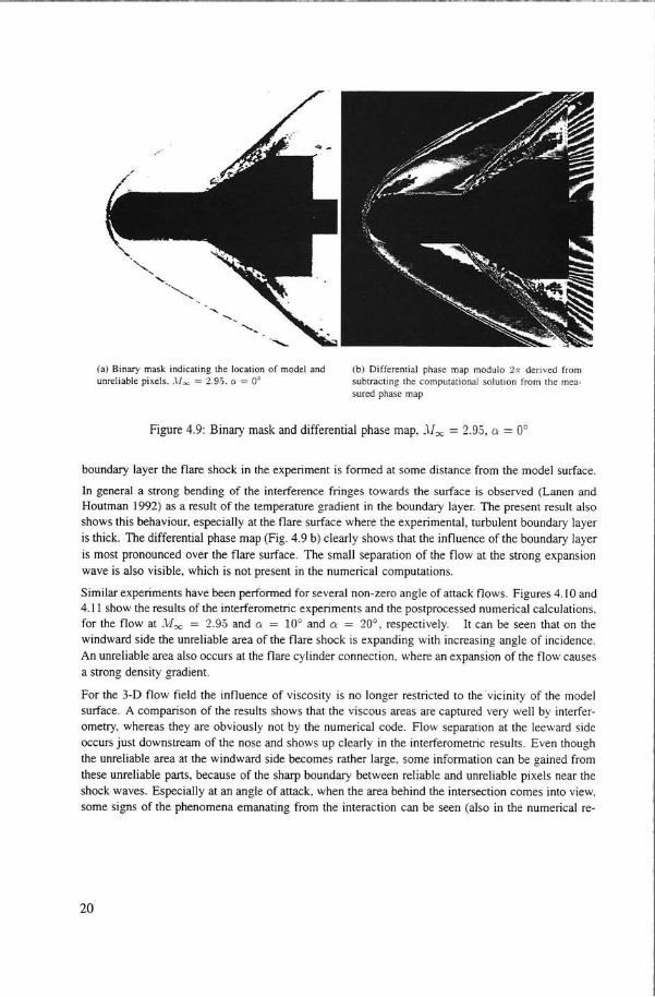
Direct comparison of measured and computed phase maps is inhibited by two error sources in the experimental data: non-uniforrnities in the free stream and the presence of unreliable areas. From the mask in Fig. 4.9 a it appears that not all pixels on the bow shock are unreliable. However, phase­unwrapping attempts fail to pass the shock correctly. Therefore in all results presented here the phase map modulo 27l" will he shown instead of the continuous ph ase map. This means that the comparison with numerical results can only reveal whether the behaviour of the flow inside the reliable areas is the same for both techniques.

18

(a) Experiment (b) Computation

Figure 4.8: Phase maps modulo 2", M x = 2.9.5, 0 = 0°

An example of a mask is given in Fig. 4.9 a for the zero angle of attack case. From the mask a strength­ening of the flare shock can be seen which is caused by the impingement of the expansion fan from the nose region due to the increase of local shock angle and Mach number. Between the nose and the bow shock the phase map modulo 2" seems to give continuous fringes , but these have to be cancelled because of unreliability.

Also the flare shocks and the shock-shock interaction area give no reliable results. An explanation for this can be found in the numerical phase map: the gradient is very high in those areas, which results in a very close spacing of the fringes, so that the limit of 2 pixels per fringe cannot be reached. This could not be helped sufficiently by zooming in on these areas. Therefore. as little or no extra information could be gained from zooming, all results are presented covering the same area: ï 5 x ï5mm2 The blurred regions at the cone surface might be due to unsteady flow phenomena, such as a turbulent boundary layer.

Fig. 4.9 b shows a pixelwise comparison by subtracting the measured and the computed phase maps. It can be seen that, apart from the shock areas, the results agree reasonably weIl. However. the dif­ferential ph ase map shows substantial differences in the vicinity of the shock waves. especially at the

bow shock near the stagnation point and at the flare shock. The numerical phàse map shows a more gradual phase difference gradient at the shock than the experimental phase map. AIso, the differential phase map is seen to be slightly asymmetric. This is caused by the fact that the angle of incidence was not exactly 0° (namely 0.45° ) and by the non-uniformity of the free stream.

Differences between the numerical and experimental phase maps can also be expected in regions of the flow field where viscous effects are present. For the axi-symmetric flow case these regions are confined to the boundary layer, which influences the flare shock. The correspondence between the shock locations is good. The results only differ at the foot of the flare shock. Due to the presence of a

19

W!'I!~"=== __ U'~"" .. __ .u ____ .. u." __ ~ __ ~ ______________ ~'~I!~-U __ ~_~'an _____ ... __ ~'''~ __ w.~-~'U-~'~''~' ___ ~-__ '~ __ ~~.~_~.w~~a,~~.w

(al Binary mask indicating the locati on of model and unreli able pixels .. H= = 2,9.'>. 0 = 0'

(bl Differemial phase map modulo 2;; denved from subtracting the computational solution from the mea· sured ph ase map

Figure 4.9: Binary mask and differential phase map, JJx = 2.95, 0. = 00

boundary layer the flare shock in the experiment is formed at some distance from the model surface.

In general astrong bending of the interference fringes towards the surface is observed (Lanen and Houtman 1992) as a result of the temperature gradient in the boundary layer. The present result also shows this behaviour, especial1y at the flare surface where the experimental, turbulent boundary layer is thick. The differential phase map (Fig. 4.9 b) clearly shows that the influence of the boundary layer is most pronounced over the flare surface. The sm all separation of the flow at the strong expansion wave is also visible, which is not present in the numeri cal computations.

Similar experiments have been performed for several non-zero angle of attack flows . Figures 4.10 and 4.11 show the results of the interferometric experiments and the postprocessed numerical calculations, for the flow at iv/x = 2.95 and 0. = 100 and Cl.' = 20 0

, respectively. It can be seen that on the windward side the unreliable area of the flare shock is expanding with increasing angle of incidence. An unreliable area also occurs at the flare cylinder connection, where an expansion of the flow causes astrong density gradient.

For the 3-D flow field the influence of viscosity is no longer restricted to the vicinity of the model surface. A comparison of the results shows that the viscous areas are captured very well by interfer­ometry, whereas they are obviously not by the numerical code. Flow separation at the leeward side occurs just downstream of the nose and shows up clearly in the interferometric results. Even though the unreliable area at the windward side becomes rather large, some information can be gained from these unreliable parts, because of the sharp boundary between reliable and unreliable pixels ne ar the shock waves. Especially at an angle of attack, when the area behind the intersection comes into view, some signs of the phenomena emanating from the interaction can be seen (also in the numerical re-

20

(a) Experiment (unreliable pixels depicted in black) (b) Computation

Figure 4.10: Phase maps modu\o 27<, lvIoe = 2.9.5, Cl = 10°

(a) Experiment (unreliable pixels depicted in black) (b) Computation

Figure 4.1 I: Phase maps modulo 2", i\lLx , = 2.9.5, Cl = 20°

21

-~~----- ~-----------------------

sults).

At the windward side of the model there is areasonabie correspondence of the experimental and nu­merical shock locations, although the numerical flare shock seems to be positioned further from the body. This may be caused by the fact that in the experimental results the flare shock is not attached to the model, whereas it is for the numerical flow field. In the experimental results the flare shock is formed closer to the model surface than for Q = 0° which is probably due to a thinner upstream boundary layer. The numerical results now yield a detached shock, which is the correct non-viscous solution. Both the numerical and the experimental resuJts show that the flare shock strength increases at the shock-shock interaction. Further downstream the flare shock becomes weaker due to the inter­action with the expansion wave originating at the cone-cylinder junction. At the leeward side of the model the flare shock is formed at a considerable di stance from the model surface due to the large scale flow separation. The non-viscous results of the Euler Code still yield a shock wave which can be traced up to the model surface.

In the interferometric measurements there seems to be some structure at the leeward side of the model aligned with the flare. Here the unreliable, flare shock area does not possess the narrow shock-like structure but has a more wavy character. Especially at an angle of 20° it gives a "vortical" impression. Topological interpretations of earlier oil-f1ow experiments reveal the presence of two counter rotating vortices originating from the separation region at the leeward side of the model (Bakker et al. 1992). which may explain this pattem. In the interferometric results these structures show up as unreliable pixels because they occur outside the symmetry plane at which the set-up is focussed. As they are not imaged properly a shadowgraph-effect occurs due to light ray deflection. Although no guantitative information can be extracted from these points, some insight into the form and behaviour of these vortical structures may be gained.

1:>.0 2rr

4 M_=2.95:a=10°

Windward ., ·20

----e----- Computation

----b- Experiment

leeward

·'0 "0

i : Sample Ijne .... [' , V , - I ______

! ~.

I 'I-~--j : , !

I I I

\ \

\ 3 E B =

20 =(mm) 3'0

Figure 4.12: Unwrapped phase along vertical line .. H 00 = 2.95. 0 = 10°

The unwrapped phase angle (!::.of27ï) along a verticalline through the cylindrical part (indicated in the sm all figure inserted) has been plotted in Figs. 4.12 and 4.13 for Q = 10° and 0 = 20°, respectively. The phase angle !::.0 is related to the integrated density along the light paths according to Eg. (2.4). The experimental phase distribution has been shifted 27ï and 4" radians for 0 = 10° and 0 = 20°,

22

~ó 211'

4 M_ = 2.95: a = 200

=

Windward ·1

·20

--e--- Computation

--8-- Experiment

-;0

i , I

11 l' Leeward

10 20

~

--lJample line '~

.~ ,

~;

=( mm J 30

Figure 4.13: Unwrapped phase along venical line.-'Ioe = 2. 9·5. 0 = 20°

respectively, in order to make a comparison with the numerical result. This shift is necessary, since the phase unwrapping in the experimental results fails at the shock due to the c10sely packed fringes. For the computations no phase unwrapping is necessary, since the ph ase angle éJ. o is a direct result of the simulation process rather than the phase modulo 2". The experimental and computational phase distribution agree rather weil in the regions which are enclosed by the model and the shock. Compar­ison of the phase distribution in the flow out si de of the shock shows that the ph ase period which has disappeared is 2" and 4" for Cl: = 10° and Cl: = 20°, respectively.

4.3 Computations

The convergence history of the computations at A100 = 2,95 and Cl: = 10° and Cl = 20° is given in Fig. 4.14. Figure 4.14(a) shows the logarithm (base 10) of the Lj-norm of the residual as a function of the FAS-iteration number. The residual drops to engineering accuracy (10-4 ) within 58 and 96 FAS iterations for Cl: = 10° and Cl: = 20° respectively. The Iift- and drag coefficients, which do not include the forces on the base area, are obtained within 0.1 % of its final value within 15 a 20 FAS-cycles. see Fig. 4. I 4(b).

Since viscous effects are not modelled by the Euler equations and the model is not equipped with sharp edges, the computational results do not predict separated flow. The bow-shock-wave topology is however predicted rather weil by the numerical method, A three-dimensiOIial view of the shock­wave pattem in the half space in the background is given in Fig. 4.15 for J\J oe = 4.04 and Cl: = 20°. In this picture the shocks are represented as surfaces. These surfaces are ca\culated by an algorithm for the detection and visualization of shocks in a discrete flow field. The criterion used for the occurrence of a shock wave is that the velocity component in the direction of the local pressure gradient should pass the sonic value. Therefore the following scalar quantity is ca\culated:

(4.1)

23

24

LoglO(Res)

.,

·3

20

M. = 2.95. Grid 64 x 48 x 32 ____ a,. 10·

___ a=20·

40 60 '0 100

FASUeralion

(a) Logarithm of L I -norm of residu al

C •. C;:

1.0

0.9

0.8

0.7

06

O.S

0.4

0.3

02

0. '

0.0

f\..-

20

M. = 2.95. Grid 64 x 48)( 32

C<.a= 100 C,. o.= 10· Cv u:E20·

Co, a=20·

40 60 '0 100

FAS Ileration

(b) CL and CD (without contribution of base area)

Figure 4.14: History of residual and aerodynamic forces, cl/Ix = 2.9.5, Cl = 10° and 20°

Figure 4.15: Shock pattem in computational data set,M"" = 4.04, ct = 20°

where q is the velocity vector, c the speed of sound and \7 p / 11\7 pil is the normalized pressure gradient. The shock surfaces are then represented as surfaces where ,Hnp = 1, and the gradient of Jifnp along the local flow direction is negative (q. \ijVInp < 0).

Besides the bow shock and the flare shock, this shock detection also reveals the existence of an em­

bedded shock at the leeward side of the conical flare. Only th is shock is also plotted in the foreground

half-space. This shock can be filtered out of the isosurface by aselection criterion which uses the nor­mal vectors of the triangular surfaces of the discrete shock surface. Only those triangles are plotted for which the angle between its normal vector and the assumed norm al vector of the shock is less than a specified value. The position of this embedded shock corresponds with a curve at which the oil-streak lines show a kink (Figs.4.5,4.7).

Figure 4.16 shows the pressure distribution in the plane of symmetry for a calculation at :"11 x = 4.04 and 0 = 20° . The bow shock is captured within 2 cells in those regions where the shock is aligned with the grid (nose region). The isobars in the region between the shock-shock interaction and the model do not reveal an adjustment shock originating from the interaction point. which was observed in the shadowgraph and also follows from the heart-diagram analysis.

M_ = 4.04; 0: = 20°

75 Range: 1.0-22.0

Step: 0.75 z

50

25

o

·25

·50

o 25 50 75 x(mm) 100 125

Figure 4.16: Isobars p/Poc in the plane of symmetry, Jfx = 4.04, Q = 20°

25

4.4 Surface pressure distributions

The surface pressure distributions obtained from the experiments and the computations at the windward- and leeward generator in the plane y = 0 are given in Figs. 4.17 - 4.20 for Mach numbers ]\1/00 = 2.95 and 4.04 and angles of attack 0 = 100 and 200. The pressure distributions from the computations agree very weil with the experimental pressure distributions in those regions which are not dominated by viscosity effects, the windward sides of the hemispherical head and the cylinder. At the leeward side of the cylinder a separation causes a higher pressure than the computations (with attached flow) predict. Furthermore, differences occur at the beginning of the f1are , where a shock-induced separation smears out the pressure increase in the experiments. At the leeward surface no shock can be observed in the experimental pressure distribution.

25 M. =2.95; a= 10°

20

15

10

Windward side

5

o

, o 20 40 60 80 x (mm)100

Figure 4.17: Computational and experimental surface pressure distribution at leeward- and windward generator, :VJoo = 2.9.5, 0 = 100

For the lower angle of attack (0 = 100), the experimental and the computational pressure distributions

at the flare agree rather weIl. In these cases the shock-shock interaction has no influence on the flare surface. Downstream of the f1are, at the cylindrical part, the decrease of pressure due to the expansion is predicted rather weil by the computational method for all angles of attack.

The effects of the shock-shock interaction on the pressure distribution at the windward side of the flare at Q = 200 are not predicted very weil by the numerical simulations. In order to explain the behaviour of the pressure distribution at the windward side at x > 80mm, the lines observed in the corresponding shadowgraphs are depicted in the Figures 4.18 and 4.20. They show that the lines coming from the interaction point, which are shocks according to the heart-diagram, coincide with a sudden increase of pressure on the surface. At Moe = 4.04 (Fig. 4.20) a significant expansion occurs just downstream of this shock, which coincides with another line coming from the interaction area and reflecting on the

26

25 M_ = 2.95; Cl = 20'

20

15

10

5

o

Lines in spark·shadowgraph

o 20 40 60 80 X (mm) 100

Figure 4.18: Computational and experimental surface pressure distribution at leeward- and windward generator, j\1= = 2.95, Ct = 20°

25 M_ = 4.04 ; Cl= 10'

20

15

10

5

o Leeward side

o 20 40 60 80 x (mm) 100

Figure 4.19: Computational and experimental surface pressure distribution at leeward- and windward generator, ,'vice = 4.04 , a = 10°

27

25 M_ = 4 .04; cr = 20'

p/p-

20

. 15

, ,

\ 10 , ,

\ . '

5 , ,

0CGUZZI 0 0 ~eeward side

0

, , ,

o 20 40 60 80 x (mm) 100

Figure 4.20: Computational and experimental surface pressure distribution at leeward- and windward generator, ]\1[= = 4.04, Q = 20°

surface. In the shadowgraph (Fig. 4.3) it is visible that this line reflects on the shear layer and again reflects on the surface, which coincides with another expansion.

The shock-shock interaction is an inviscid phenomenon, which should be modelled by the present numerical method. The weak adjustment shocks and expansion waves are not captured due to the numerical dissipation, which causes discontinuities to be smeared out when they are not aligned with grid lines. A finer grid in the x-direction (96 cells) with a clustering of points near the shock-shock interaction did not improve the result. The pressure distributions at the f1are for the standard and the finer grid computations and the experiment are shown in Fig. 4.21 .

The embedded shock at the f1are, which was predicted by the shock detection algorithm, can also be observed in the computational leeward surface pressure distribution, which is given in the upper half of Fig. 4.22 together with some streamlines. The kink in the streamlines at this shock are also ob­served in the oil-f1ow visualization (Figs.4.5,4.7). The experimental pressure distribution, which is given in the lower half of Fig. 4.22, does not show the shock; apparently, the pressure rise through the shock is smeared out and decreased by the (turbulent) boundary layer. At the windward side the com­putational and experimental pressure distributions agree rather weil at the cylindrical part (Fig. 4.23); at the f1are the effect of the adjustment shock is not visible in the computational pressure distribu­tion, The footprint of the adjustment shock in the experimental pressure distribution may be observed by the local maxima. The shape of this footprint is almost identical to the footprint observed in the oil-f1ow visualization (Fig. 4.6).

28

25 M_ = 4.04; a = 20'

15

10

5

o

60

leeward side

80

] Experiment

-==J Comp. 64)(48)(32

-==J Comp. 96)(48x48

x (mm) 100

Figure 4.21: Computational and experimental surface pressure distribution at the leeward and wind­ward generator of the flare, !1100 = 4.04, Q = 20°

M_ = 4.04; Cr. = 20°; lsobars p/p,~; Increment = 0.2

Leeward side

Computation

Experiment

Figure 4.22: Computational and experimental leeward surface pressure distribution, JI[= = 4.04, Q = 20°

29

M_ = 4.04 : a = 20°: lsobars p/p~: Increment = 0. 5

Windward side

Computation

Experiment

Figure 4.23: Computational and experimental windward surface pressure distribution, 1\10:; = 4.04, Oe = 20°

30

Chapter 5

CONCLUSIONS

Different experimental techniques have been used to analyse the high-supersonic flow around a hemispherical-nose-cylinder with conical flare. The model has been investigated for flows with free-stream Mach numbers of 3 and 4 and angles of attack from 0° up to 20° . Interesting features of this flow are a complex surface flow topology. with various separalions and their interactions, and a shock-shock interaction at large angles of attack in the windward region interfering with the body. The experiments are compared with computational results obtained from an Euler code.

Qualitative visualization techniques as spark shadowgraph and surface oil-flow appear to be a valuable tooi to identify characteristic features about the flow topology and the shock pattems. High resolution surface pressure data support the interpretation of the visualization studies.

Digital Holographic Interferometry is a valuable tooi for quantitative flow diagnostics. since the entire integrated density field is captured at a single moment. It may serve as a validation instrument for computer codes. because the integrated density can be compared direclly 10 post-processed numerical results . Difficult areas in the flow field are areas with high density gradients (shock waves) normal to the light rays, where the phase-unwrapping process fails. Simulated ph ase maps were obtained from discrete solutions of a 3D Euler code, neglecting the light ray deflection. The experimental results and the post-processed Euler results show a rather good agreement in those areas which are not affected by viscous effects or by shock waves. Comparing interferometric and numerical results can serve multiple purposes, as differences may reveal flaws in both methods and can assist in mutual interpretation of the results. Comparison of both phase maps gives some insight into the possible causes for "bad" points in the interferometric results. E.g., the Euler code results reveal that the areas indicated as unreliable in the interferometry (because of low modulation intensity) near the shock waves and expansion areas at the flare-cylinder junction are caused by astrong density gradient, so that the sampling condition cannot be met.

The computational results are compared with detailed surface pressure measurements. The pressure distribution at the nose and the windward side of the model is predicted rather weil by the Euler code. At the leeward side, where the flow is dominated by the presence of separation and vortex formation . the agreement between experimental pressure and computational pressures is rather poor. as ma)' be expected. The surface pressure distributions at 20Q angle of attack indicate adjustment shocks and expansion waves originating from the shock-shock interaction in the windward flow field. The ad­justment shock- and expansion waves, which interfere with the body. are however not captured by the numerical method due to numerical dissipation. In order to capture these phenomena. a very fine grid in the shock-shock interaction region should be used.

31

REFERENCES

ANDERSON, W.K., THOMAS, J.L. , AND WHITFIELD, D.L. (1988) "Multigrid Acceleration of the Flux-split Euler Equations," A1AA Joumal, 26(6):649-654.

BAKKER, P.G. AND BANNINK, W.J. (1992) "Experimental Visualization of Viscous Interaction Effects in Compressible Flow Field," Annual report 1992, pp. 18-28, I.M. Burgers Centre for Fluid Mechanics.

BAKKER , P.G., BAN NINK , W.J ., AND L USSE. P.A. (1992) "Experimental lnvestigation of the High Supersonic Flowfield past a Re-entry Body," In Brun, R. and Chikhaoui, A.A. , editors, /UTAM Symposium: Aerothermochemistry of Spacecrafts and Associated Hypersonic Flows, pp. 413-418, Marseille.

BAN NINK , W.L (1963) "De verdeling van het getal van Mach bij een beperkt gedeelte van de meet­plaats van de supersone wind tunnel no. 2 bij een nominaal getal van Mach van 3." Memorandum m-75, Dept. of Aerospace Engineering, Delft University of Technology.

EDNEY, B. (1968) "Anomalous Heat Transfer and Pressure Distributions on Blunt Bodies at Hyper­

sonic Speeds in the Presence of an Impinging Shock," FFA Report 115, The Aeronautical Research Institute of Sweden.

FRA NÇON, M . (1974) "Holography, " Academic Press, New York.

HEMKER, P.W. AND KOREN , B . (1995) "Defect Correction and Nonlinear Multigrid for the Steady Euler Equations," In Habashi, W.G. and Hafez, M.M., editors, Compurarional Fluid Dynamics Tech­niques, pp. 699 - 718. Gordon and Breach, Base!.

LANEN, TH.A.W.M. (1992) "Digiral Holographic Interferometry in Compressible Flow Re­search, " PhD thesis, Delft University of Technology.

LANEN, T.A.W.M., BAKKER, P.G. , AND BRYANSTO N-CROSS, P.J . (1992) "Digital Holographic Interferometry in High-Speed Flow Research," Experiments in Flt/ids, 13:56-62.

L ANEN, T. AND HO UTMA N, E.M. (1992) "Comparison oflnterferometric Measurements with 3-D Euler Computations for Circular Cones in Supersonic Flow," AIAA Paper 92-2691 CP.

L ANEN. T.A.W.M., NEBBELI NG, c. , AN D IN GE N, J .L. VAN (1990) "Phase-stepping Holographic Interferometry in Studying Transparent Density Fields around 2-D Objects of Arbitrary Shape," Opr. Comm., 76:268-276.

LEER, B. VAN (1977) "Towards the Ultimate Conservation Difference Scheme IV; A New Approach to Numerical Convection," Joumal of Camp. Physics, 23:276--299.

LEER, B. VA N (1982) "Flux-Vector Splitting for the Euler Equations," Lecture Notes in Physics, 170:507-512.

LUSSE, P. (1992) "Visualisation Study of a Blunt-Cylinder-Flare Model in High Supersonic Flow," Graduate thesis, Dept. of Aerospace Engineering, Delft University of Technology.

32

MONTGOMERY, G.P. AND REUSS. D.L. (1982) "Effects of Refraction on Axisymmetric Flame Temperatures measured by Holographic Interferometry," Appl. Opr. , 21 :1373-1380.

OSHER, S. AND SOLOMON , F. (1982) "Upwind Difference Schemes for Hyperbolic Systems of Conservation Laws," Marh. Camp., 38:339-374.

REGINATO, S. (1993) "Pressure Measurements on a Blunt-Cylinder-Flare Model in High Supersonic Flow," Graduate thesis, Delft University of Technology/ University of Pisa.

ROE , P.L. (1981) "Approximate Riemann Solvers, Parameter Vectors and Difference Schemes," Joumal of Camp. Physics, 43:357-372.

SPEKREIJSE, S.P. (1987) "Mulrigrid SoLurion of rhe Sready EuLer Equariolls. " PhD thesis, Delft University of Technology.

33

Series 01: Aerodynamics

01. F. Motallebi, 'Prediction of Mean Flow Data for Adiabatic 2-D Compressible Turbulent Boundary Layers' 1997 / VI + 90 pages / ISBN 90-407-1564-5

02. P.E. Skare, 'Flow Measurements for an Afterbody in a Vertical Wind Tunnel' 1997 / XIV + 98 pages / ISBN 90-407-1565-3

03. B.W. van Oudheusden, 'Investigation of Large-Amplitude 1-DOF Rotational Galloping' 1998 / IV + 100 pages / ISBN 90-407-1 566-1

04. E.M. Houtman / W .J. Bannink / B.H. Timmerman, 'Experimental and Computational Study of a Blunt Cylinder-Flare Model in High Supersonic Flow' 1998 / VIII + 40 pages / ISBN 90-407-1567-X

05. G.J .D. Zondervan, 'A Review of Propeller Modelling Techniques Based on Euler Methods' 1998/ IV + 84 pages / ISBN 90-407-1568-8

06. M .J. Tummers / D.M. Passchier, 'Spectral Analysis of Individual Realization LDA Data' 1998/ VIII + 36 pages / ISBN 90-407-1569-6

07. P.J.J. Moeleker, 'Linear Temporal Stability Analysis' 1998/ VI + 74 pages / ISBN 90-407-1570-X

08. B.W. van Oudheusden, 'Galloping Behaviour of an Aeroelastic Oscillator with Two Degrees of Freedom' 1998 / IV + 128 pages / ISBN 90-407-1571-8

09. R. Mayer, 'Orientation on Quantitative IR-thermografy in Wall-shear Stress Measurements' 1998 / XII + 108 pages / ISBN 90-407-1 572-6

10. K.J.A. Westin / R.A.W.M. Henkes, 'Prediction of Bypass Transition with Differential Reynolds Stress Modeis ' 1998/ VI + 78 pages / ISBN 90-407-1573-4

11. J.L.M . Nijholt, 'Design of a Michelson Interferometer for Quantitative Refraction Index Profile Measurements' 1998/ 60 pages / ISBN 90-407-1574-2

12. R.A.W.M. Henkes / J .L. van Ingen, 'Overview of Stability and Transition in External Aerodynamics' 1998/ IV + 48 pages / ISBN 90-407-1575-0

13. R.A.W.M. Henkes, 'Overview of Turbulence Models for External Aerodyna­mics' 1998 / IV + 40 pages / ISBN 90-407-1576-9

Series 02: Flight Mechanics

01. E. Obert, 'A Method for the Determination of the Effect of Propeller Slip­stream on a Stattc Longitudinal Stability and Control ot Multi-engined Aircraft' 1997/ IV + 276 pages / ISBN 90-407-1577-7

02. C. Bill / F. van Dalen / A. Rothwell, 'Aircraft Design and Analysis System (ADAS)' 1997 / X + 222 pages / ISBN 90-407-1578-5

03. E. Torenbeek, 'Optimum Cruise Performance of Subsonic Transport Air­craft' 1998 / X + 66 pages / ISBN 90-407-1579-3

Series 03: Control and Simulation

01. J.C. Gibson, 'The Definition, Understanding and Design of Aircraft Handling Qualities' 1997 / X + 162 pages / ISBN 90-407-1580-7

02. E.A. Lomonova, 'A System Look at Electromechanical Actuation for Primary Flight Control' 1997 / XIV + 110 pages / ISBN 90-407-1581-5

03. C.A.A.M. van der Linden, 'DASMAT-Delft University Aircraft Simulation Model and Analysis TooI. A Matlab/Simulink Environment for Flight Dyna­mics and Control Analysis' 1998 / XII + 220 pages / ISBN 90-407-1582-3

Series 05: Aerospace Structures and Computional Mechanics

01. A .J. van Eekelen, 'Review and Selection of Methods for Structural Reliabili­ty Analysis' 1997 / XIV + 50 pages / ISBN 90-407-1583-1

02. M.E. Heerschap, 'User's Manual for the Computer Program Cufus. Quick Design Procedure for a CUt-out in a FUSelage version 1.0' 1997 / VIII + 144 pages / ISBN 90-407-1584-X

03. C. Wohlever, 'A Preliminary Evaluation of the B2000 Nonlinear Shell Element Q8N.SM' 1998/ IV + 44 pages / ISBN 90-407-1585-8

04. L. Gunawan, 'Imperfections Measurements of a Perfect Shell with Specially Designed Equipment (UNIVIMP) 1998 / VIII + 52 pages / ISBN 90-407-1586-6

I \

Series 07: Aerospace Materials

01 . A. Vasek / J. Schijve, 'Residual Strenght of Cracked 7075 T6 AI-alloy Sheets under High Loading Rates' 1997 / VI + 70 pages / ISBN 90-407-1587-4

02. I. Kunes, 'FEM Modelling of Elastoplastic Stress and Strain Field in Centre­cracked Plate' 1997 / IV + 32 pages / ISBN 90-407-1588-2

03. K. Verolme, 'The Initial Buckling Behavior of Flat and Curved Fiber Metal Laminate Panels' 1998 / VIII + 60 pages / ISBN 90-407-1589-0

04. P.W.C. Provó Kluit, 'A New Method of Impregnating PEl Sheets for the /n­Situ Foaming of Sandwiches ' 1998 / IV + 28 pages / ISBN 90-407-1590-4

05. A. Vlot / T. Soerjanto / I. Yeri / J .A . Schelling, 'Residual Thermal Stress es around Bonded Fibre Metal Laminate Repair Patches on an Aircraft Fusela­ge' 1998/ IV + 24 pages / ISBN 90-407-1591-2

06 . A. Vlot, 'High Strain Rate Tests on Fibre Metal Laminates' 1998/ IV + 44 pages / ISBN 90-407-1592-0

07. S. Fawaz, 'Application of the Virtual Crack Closure Technique to Calculate Stress Intensity Factors for Through Cracks with an Oblique Elliptical Crack Front' 1998/ VIII + 56 pages / ISBN 90-407-1593-9

08. J. Schijve, 'Fatigue Specimens for Sheet and Plate Material' 1998/ VI + 18 pages / ISBN 90-407-1594-7

Series 08: Astrodynamics and Satellite Systems

01. E. Mooij. 'The Motion of a Vehicle in a Planetary Atmosphere' 1997 / XVI + 156 pages / ISBN 90-407-1595-5

02. G.A. Bartels, 'GPS-Antenna Phase Center Measurements Performed in an Anechoic Chamber' 1997 / X + 70 pages / ISBN 90-407-1596-3

03. E. Mooij. 'Linear Quadratic Regulator Design for an Unpowered, Winged Re­entry Vehicle' 1998/ X + 154 pages / ISBN 90-407-1597-1

)01- 1 8&1

The high supersonic flow around a generic re-entry body (hemisphericalnose-cylinder with conical flare) at incidence has been investigated experimentally and numerically. Visualization studies using shortexposure shadowgraphy and surface oil-flow have provided a qualitative understanding of the flow physics. Quantitative results are obtained with a holographic interferometry system with digital image processing. These results are compared with post-processed numerical data from inviscid flow simulations with a 30 Euler code. Extensive surface pressure measurements deliver a detailed pressure distribution on the body which can be used as a validation of computational codes. Interesting features of the flow are a complex surface flow topology at the leewards side with various separations, and a shock-shock interaction in the windward reg ion interfering with the body.

I SBN 90-407 - 1S67 -X

DELFT AEROS~"'~~ 9 78 fN G IN E ERING & TE C HNOLOGY