studies on genetics of heat stress in us holsteins … · studies on genetics of heat stress in ......
TRANSCRIPT
STUDIES ON GENETICS OF HEAT STRESS IN US HOLSTEINS
by
JARMILA BOHMANOVA
(Under the Direction of Ignacy Misztal)
ABSTRACT
The objective of this study was to explore the genetic component of heat stress in U.S.
Holsteins using national milk yield data consisting of 57 million first-parity test-day records of 6
million Holstein cows that calved from 1993 through 2004 and weather records from 202 public
weather stations.
Seven temperature humidity indices were compared in a humid and semi-arid climate for
their ability to detect a decline of milk yield due to heat stress. The index with a higher weight on
humidity was the best in the humid climate. The index with a larger weight on temperature was
the best heat stress indicator in the semi-arid climate.
National genetic evaluation for heat tolerance was conducted using a repeatability test-
day model. Based on estimated heat tolerance PTAs, the 100 most and 100 least heat-tolerant
sires were selected. For each of the 200 sires, official U.S. PTAs from February 2006 were
obtained. Sires that were the most heat tolerant transmitted lower milk yields with higher fat and
protein contents than did sires that were the least heat tolerant. Daughters of the most heat
tolerant sires had better udder and body composition, better type, lower dairy form, slightly
higher TPI, longer productive life, higher daughter pregnancy rate, were easier calving and had
better persistency than did daughters of the least heat tolerant sires.

Heat stress was evaluated as a factor in the genotype x environment interaction on milk
production in the United States. Data for the Southeast and Northeast were extracted from the
national data set and analyzed separately. Two repeatability models with and without the effect
of heat stress were implemented. Both models were fitted with the national and regional data
sets. Correlations between breeding values of sires with ≥ 100 and ≥ 300 daughters in two
regions were calculated. When heat stress was ignored (first model), the correlation of regular
breeding values between regions for sires with ≥ 100 (≥ 300) daughters was 0.85 (0.87). Heat
stress as modeled here explains only a small amount of genotype by environment interaction,
partly because test day records provide only snapshots of heat stress over a hot season.
INDEX WORDS: Dairy cattle, Genetic evaluation, Genotype by environment interaction,
Holstein, Heat stress, Milk yield, Temperature humidity index

STUDIES ON GENETICS OF HEAT STRESS IN US HOLSTEINS
by
JARMILA BOHMANOVA
M.S., Czech University of Agriculture, Czech Republic, 2001
A Dissertation Submitted to the Graduate Faculty of The University of Georgia in Partial
Fulfillment of the Requirements for the Degree
DOCTOR OF PHILOSOPHY
ATHENS, GEORGIA
2006

© 2006
Jarmila Bohmanova
All Rights Reserved

STUDIES ON GENETICS OF HEAT STRESS IN US HOLSTEINS
by
JARMILA BOHMANOVA
Major Professor: Ignacy Misztal
Committee: Romdhane Rekaya J. Keith Bertrand
Joe W. West Electronic Version Approved: Gerrit HoogenboomMaureen Grasso
Dean of the Graduate School The University of Georgia May 2006

iv
ACKNOWLEDGEMENTS
I would like to express my deepest gratitude to Dr. Ignacy Misztal for his critical
guidance and invaluable assistance. It has been a pleasure and honor to work with him during the
course of my programs. Many thanks must also go to members of my committee; Drs.
Romdhane Rekaya, Keith Bertrand, Joe West and Gerrit Hoogenboom for their advice and
assistance.
I wish to thank the past and current members of Animal Breeding and Genetics group at
UGA for providing friendly and enthusiastic environment. In particular, I would like to thank
Drs. Shogo Tsuruta, Jesus Arango, Saidu Oseni, Andres Legarra, Kath Donoghue, and Robyn
Sapp for their friendship and assistance. Special thanks must go to Brenda Burke for her
friendship, encouragement and teaching me ‘the correct way of talking’. I also want to thank
Mike Kelley for his technical support over the years. It has been a pleasure to spend time with
such a wonderful group of people.
The friendship and assistance of Carolina Realini, Jorge Urioste, Ignacio Aguilar and
Mary Orwig is greatly appreciated. Conversations with Drs. Tom Lawlor, John Cole and Dean
Roger have been beneficial and enjoyable.
I would like to thank my friends in the Czech Republic for their encouragement and
stimulation. Finally, special thanks must go to my parents, brother and his wife and my
grandparents for their invaluable and unconditional love, support and encouragement.

v
TABLE OF CONTENTS
Page
ACKNOWLEDGEMENTS............................................................................................... iv
LIST OF TABLES........................................................................................................... viii
LIST OF FIGURES ............................................................................................................ x
CHAPTER
1 INTRODUCTION .................................................................................................. 1
2 REVIEW OF LITERATURE ................................................................................. 3
Thermoneutral zone .................................................................................... 3
Defining heat stress..................................................................................... 5
Response to heat stress................................................................................ 6
Heat exchange............................................................................................. 7
Physiological responses to exposure to thermal stress ............................... 8
Climatic heat stress factors ....................................................................... 12
Factors influencing heat tolerance ............................................................ 15
Methods for assessment of heat tolerance ................................................ 20
Characteristics of a heat tolerant animal................................................... 24
Strategies for reduction of effects of heat stress ....................................... 25
Literature Cited ......................................................................................... 29
3 COMPARISON OF SEVEN TEMPERATURE HUMIDITY INDICES AS
INDICATORS OF MILK PRODUCTION LOSSES DUE TO HEAT STRESS IN
SEMI-ARID AND HUMID CLIMATES............................................................. 38
vi
Abstract ..................................................................................................... 39
Introduction............................................................................................... 39
Data and Methods ..................................................................................... 45
Results....................................................................................................... 51
Conclusions............................................................................................... 52
Literature Cited ......................................................................................... 52
4 NATIONAL GENETIC EVALUATION OF MILK YIELD FOR HEAT
TOLERANCE OF UNITED STATES HOLSTEINS .......................................... 73
Introduction............................................................................................... 74
Materials and Methods.............................................................................. 76
Results....................................................................................................... 78
Conclusions............................................................................................... 80
Acknowledgements................................................................................... 80
References................................................................................................. 80
5 HEAT STRESS AS A FACTOR IN GENOTYPE X ENVIRONMENT
INTERACTION IN U.S. HOLSTEINS................................................................ 86
Abstract ..................................................................................................... 87
Introduction............................................................................................... 88
Materials and methods .............................................................................. 90
Results and discussion .............................................................................. 93
Conclusions............................................................................................... 95
Acknowledgments..................................................................................... 96

vii
References................................................................................................. 97
6 CONCLUSIONS................................................................................................. 107

viii
LIST OF TABLES
Table 3.1: Dew point temperature (Tdp in °C) for dry bulb temperature (Tdb) between 20 and 34
°C and relative humidity between 50 and 100%........................................................................... 54
Table 3.2: Wet bulb temperature (Twb in °C) for dry bulb temperature (Tdb) between 20 and 34
°C and relative humidity between 50 and 100%........................................................................... 54
Table 3.3: TH1 for dry bulb temperature (Tdb) between 20 and and 34 °C and relative humidity
between 50 and 100% ................................................................................................................... 54
Table 3.4: TH2 for dry bulb temperature (Tdb) between 20 and 34 °C and relative humidity
between 50 and 100% ................................................................................................................... 55
Table 3.5: TH3 for dry bulb temperature (Tdb) between 20 and 34 °C and relative humidity
between 50 and 100% ................................................................................................................... 55
Table 3.6: TH4 for dry bulb temperature (Tdb) between 20 and 34 °C and relative humidity
between 50 and 100% ................................................................................................................... 55
Table 3.7: TH5 for dry bulb temperature (Tdb) between 20 and 34 °C and relative humidity
between 50 and 100% ................................................................................................................... 56
Table 3.8: TH6 for dry bulb temperature (Tdb) between 20 and 34 °C and relative humidity
between 50 and 100% ................................................................................................................... 56
Table 3.9: TH7 for dry bulb temperature (Tdb) between 20 and 34 °C and relative humidity
between 50 and 100% ................................................................................................................... 56
Table 3.10: Descriptive statistics of weather data from Athens and Phoenix .............................. 57
Table 3.11: Descriptive statistics of performance data (1993-2004) from herds nearby Athens
and Phoenix................................................................................................................................... 58

ix
Table 3.12: Threshold of heat stress and rate of decline (α ) of milk production (in kg) due to
heat stress for seven THIs ............................................................................................................. 58
Table 3.13: Ratio of Twb and Tdb (Twb :Tdb) in THI1-THI7, yearly heat stress degrees and yearly
losses (Δy) in milk production due to heat stress detected by THI1-THI7 in Athens and Phoenix,
rank of THI based on Δy............................................................................................................... 58
Table 4.1: Average PTAs and TPIs from February 2006 U.S. official evaluation for the 100 most
and 100 least heat tolerant U.S. Holstein bulls ............................................................................. 82
Table 4.2: Summary of average state milk and heat tolerance PTA, rank of states based on milk
and heat tolerant PTAs and number of cows included in the evaluation per state ....................... 83
Table 5.1: Summary statistics of national and regional data sets ................................................. 99
Table 5.2: Number of weather stations per state, average (Mean), minimal (Min), maximal (Max)
and standard deviation (SD) of yearly heat stress degrees per state ........................................... 100
Table 5.3: Average number of daughters per sire for 636 sires with ≥ 100 daughters and for 265
sires with ≥ 300 daughters in National, Northeast and Southeast data set. ................................ 104
Table 5.4: Spearman correlations of sire’s breeding values for heat tolerance additive effect
(Corra1_GE), generic additive effect (Corra0_GE) using the Expanded model and generic additive
effect (Corra_G) using the Standard model between Southeast (SE), Northeast (NE) and National
(NE) data sets; differences in correlations of generic additive effects from the Expanded model
and the Standard model (Corra0_GE - Corra_G).............................................................................. 105
Table 5.5: Spearman correlations of original (as estimated in NA), and altered state specific
breeding values (breeding values for heat stress four times larger - in parentheses) ................. 106
x
LIST OF FIGURES
Figure 2.1: Diagram of the relationship between ambient temperature and heat production
(adapted from Yousef (1985) and Curtis (1981)) ........................................................................... 4
Figure 3.1: Average diurnal pattern of January dry bulb temperature (Tdb in °C) and relative
humidity (RH in %) in Phoenix and Athens ................................................................................. 59
Figure 3.2: Average diurnal pattern of June dry bulb temperature (Tdb in °C) and relative
humidity (RH in %) in Phoenix and Athens ................................................................................. 60
Figure 3.3: Average monthly pattern of dry bulb temperature (Tdb in °C) and relative humidity
(RH %) in Athens and Phoenix..................................................................................................... 61
Figure 3.4 Average monthly pattern of wet bulb depression (WBD in °C) in Phoenix and Athens
....................................................................................................................................................... 62
Figure 3.5: Average June diurnal pattern of temperature humidity indices (THI 1- THI 7) in
Phoenix ......................................................................................................................................... 63
Figure 3.6: Average June diurnal pattern of seven temperature humidity indices (THI1-THI7) in
Athens ........................................................................................................................................... 64
Figure 3.7: Average monthly pattern of THI1- THI7 in Phoenix................................................. 65
Figure 3.8: Average monthly pattern of THI1- THI7 in Athens................................................... 66
Figure 3.9: Seasonal differences in milk production in herds near Athens and Phoenix ............. 67
Figure 3.10: Temperature humidity index (THI5) with (cooled) and without (not cooled)
accounting for use of evaporative cooling .................................................................................... 68
Figure 3.11: Least square estimates (x), regression on degrees of THI1 (solid line), a threshold of
heat stress and a slope of decline of milk yield in Phoenix .......................................................... 69

xi
Figure 3.12: Least square estimates (x), regression on degrees of THI1 (solid line), a threshold of
heat stress and a slope of decline of milk yield in Athens ............................................................ 69
Figure 3.13: Least square estimates (x), regression on degrees of THI2 (solid line), a threshold of
heat stress and a slope of decline of milk yield in Phoenix .......................................................... 69
Figure 3.14: Least square estimates (x), regression on degrees of THI2 (solid line), a threshold of
heat stress and a slope of decline of milk yield in Athens ............................................................ 69
Figure 3.15: Least square estimates (x), regression on degrees of THI3 (solid line), a threshold of
heat stress and a slope of decline of milk yield in Phoenix .......................................................... 70
Figure 3.16: Least square estimates (x), regression on degrees of THI3 (solid line), a threshold of
heat stress and a slope of decline of milk yield in Athens ............................................................ 70
Figure 3.17: Least square estimates (x), regression on degrees of THI4 (solid line), a threshold of
heat stress and a slope of decline of milk yield in Phoenix .......................................................... 70
Figure 3.18: Least square estimates (x), regression on degrees of THI4 (solid line), a threshold of
heat stress and a slope of decline of milk yield in Athens ............................................................ 70
Figure 3.19: Least square estimates (x), regression on degrees of THI5 (solid line), a threshold of
heat stress and a slope of decline of milk yield in Phoenix .......................................................... 71
Figure 3.20: Least square estimates (x), regression on degrees of THI5 (solid line), a threshold of
heat stress and a slope of decline of milk yield in Athens ............................................................ 71
Figure 3.21: Least square estimates (x), regression on degrees of THI6 (solid line), a threshold of
heat stress and a slope of decline of milk yield in Phoenix .......................................................... 71
Figure 3.22: Least square estimates (x), regression on degrees of THI6 (solid line), a threshold of
heat stress and a slope of decline of milk yield in Athens ............................................................ 71

xii
Figure 3.23: Least square estimates (x), regression on degrees of THI7 (solid line), a threshold of
heat stress and a slope of decline of milk yield in Phoenix .......................................................... 72
Figure 3.24: Least square estimates (x), regression on degrees of THI7 (solid line), a threshold of
heat stress and a slope of decline of milk yield in Athens ............................................................ 72
Figure 4.1: Trend of PTAs for daughter pregnancy rate (DPR) and heat tolerance by year of birth
....................................................................................................................................................... 84
Figure 4.2: Trend of test-day PTA’s in thermal and temperate conditions and 305 day PTA’s by
bull’s birth year ............................................................................................................................. 85
Figure 5.1: Proportional distribution of test day records in the Southeastern data set by state .. 101
Figure 5.2.Proportional distribution of test day records in the Northeast data set by state ........ 102
Figure 5.3: Frequency of test day records with no heat stress (avgTHI <72), moderate heat stress
(73 ≤ avgTHI ≤ 76) and severe heat stress (avgTHI > 76) in National, Northeast and Southeast
data set ........................................................................................................................................ 103

1
CHAPTER
CHAPTER 1
INTRODUCTION
Heat stress is one of the major factors that has a negative impact on milk production and
reproduction of Holstein cattle in the southern part of United States. The impact of heat stress
can be relieved by modification of the environment (nutrition, cooling) or by genetic selection of
animals less affected by thermal stress. Identification of such animals can be based on
measurements of their immediate response (rectal, skin, milk temperature, respiration rate) to the
exposure to heat stress conditions. However, it is impossible to use these variables in a breeding
program because the collecting of such records on a national basis would be very tedious and
labor intensive. Alternatively, a decline of production due to heat stress can be used as an
indicator of heat tolerance. In Holsteins, test-day milk yield is an obvious choice. The animal
with a minimal decline of milk production per degree of increase of a climatic variable is
identified as heat tolerant. Dry bulb temperatures combined with humidity in an index are
usually used for the description of climatic conditions because of their availability from public
weather stations. Meteorological data from public weather stations provide an accurate
description of environmental conditions on farms even kilometers away. Nevertheless, if cooling
devices are used on the farm, the actual climatic conditions in the barn are different from those at
the weather station. This fact can significantly mask the real effect of heat stress. However,
accounting for the effect of cooling is compromised by a lack of adequate records on the use and
efficiency of these heat abatement devices.

2
The first objective of this study was to identify the best temperature humidity index
suitable for studying heat stress in Holsteins. Currently seven different indices are available but
none of them was specifically designed for Holstein cattle. The second objective was to conduct
a genetic evaluation for heat stress and identify genetically superior sires for heat tolerance and
investigate their genetic value in yield and non-yield traits. The third objective was to investigate
whether heat stress is a factor in the genotype by environment interaction for milk production in
the United States.

3
CHAPTER 2
REVIEW OF LITERATURE
Cattle, as other homeothermic animals, require relatively constant core body temperature
for their vital and productive processes. The body temperature of homeothermic animals is
relatively uniform, fluctuating around 39°C. But since extensive metabolic heat is produced by
internal organs, the core is usually warmer than the shell. Body temperature also varies with the
time of the day, tending to be lower in the morning and higher in the late afternoon and early
evening. Diurnal variation of body temperature doesn’t exceed 1°C if the animal is exposed to a
natural environment. The highest increase of body temperature occurs after feeding (Yousef,
1985). In cows, body temperature varies with the stage of lactation, level of milk production,
physical activity and stage of the estrous cycle (Curtis, 1983; Shearer and Beede, 1990b).
The best single indicator of average body temperature is probably blood temperature in
the aorta since it represents a mixture of blood from all over the body. Rectal temperature
estimates average body temperature less accurately because it changes more slowly than average
body temperature (Curtis, 1983). Igono et al. (1987) reported that milk temperature is a practical
measurement for assessment of heat stress in dairy cattle.
Thermoneutral zone
Thermoneutral zone (comfort zone) is the range of ambient temperature within which
metabolic rate is at a minimum, and within which temperature regulation is achieved by

4
nonevaporative physical processes alone. The most comfortable range of environmental
temperatures for milk production of dairy cattle is between 0 and 16°C (Yousef, 1985).
As shown in Figure 2.1, the thermoneutral zone is bounded by the lower critical
temperature (LCT), which is defined as the ambient temperature below which the rate of
metabolic heat production increases by shivering and (or) nonshivering thermogenic processes to
maintain thermal balance. The upper end of the thermoneutral zone, at which the increase in heat
production is primarily due to a rise in body temperature, is called the upper critical temperature
(UCT). The UCT is also defined as the ambient temperature above which thermoregulatory
evaporative heat loss processes are activated (Yousef, 1985).
Figure 2.1: Diagram of the relationship between ambient temperature and heat production (adapted from
Yousef (1985) and Curtis (1981))
Heat stress
Thermoneutral zone
Cold stress
UCT LCT
Cool Thermal comfort
Warm
Ambient temperature
Hea
t pro
duct
ion
The thermoneutral zone is subdivided into three subzones: cool, thermal comfort, and
warm. The cool zone is the range of ambient temperature where heat production remains
5
minimal and the animal conserves energy by cover insulation (piloerection), tissue insulation
(peripheral vasoconstriction) and cold induced heat production (shivering). The thermal comfort
zone is the range of ambient temperature where optimum productivity, efficiency, and
performance is demonstrated. The warm zone is the range of ambient temperature where heat
production is minimal, and the thermoregulatory responses are limited to decreasing tissue
insulation by vasodilatation and increasing the effective surface area by changing posture
(Curtis, 1983; Yousef, 1985).
The lower critical temperature (LCT) varies and dependends upon age, nutrition, level of
production, specific housing and pen conditions, breed type, behavior, and acclimatization.
Upper critical temperature is less variable and depends on the degree of acclimatization, rate of
production, pregnancy status, air movement around animals, and relative humidity (Fuquay,
1981; Shearer and Beede, 1990a; Young, 1981).
When ambient temperature rises above the upper critical temperature (UCT), the animal
can no longer control its body temperature, and the hypothalamic thermoregulatory center sends
signals to induce a sequence of thermoregulatory responses increasing peripheral blood flow
from internal organs to peripheral tissues, sweating, and panting, reducing feed intake and
nutrient absorption (Shearer and Beede, 1990b). The active dissipation processes (sweating and
panting) require the expenditure of considerable amount of energy, hence in the heat stress zone
the animal’s heat production rises above the minimal level (Curtis, 1983).
Defining heat stress
Stress denotes the magnitude of external forces which tend to displace the bodily system
from its resting or ground state (Yousef, 1985). Stress may be climatic, such as extensive cold or
heat; nutritional, due to feed or water deprivation; social, resulting from a low rank in the

6
pecking order or internal, due to some physiological disorder, pathogens or toxins (Stott, 1981).
Strain is described as the displacement from the resting or ground state by internal forces
(Yousef, 1985). Heat stress occurs when any combination of environmental factors cause the
effective temperature of the environment to be higher than the animal’s thermoneutral zone
(Armstrong, 1994). Stress from the thermal environment is a major factor negatively affecting
production and reproduction of dairy cattle. Annual economic losses of the US dairy industries
caused by heat stress average $897 million (St-Pierre et al., 2003). Because of the major
significance of this problem, heat stress in dairy cattle has been extensively discussed by many
authors (Bianca, 1965; Garcia-Ispierto et al., 2006; Kadzere et al., 2002; Nienaber et al., 1999;
Shearer and Beede, 1990a; Shearer and Beede, 1990b; St-Pierre et al., 2003; West, 2003; Yousef,
1985) in the last several decades.
Response to heat stress
Adaptation is a change which reduces the physiological strain produced by a stressful
component of the total environment. Two types of adaptations are recognized:
1. Genetic adaptation – a genetically fixed condition of a specie, which favors survival in a
particular environment
2. Phenotypic adaptation - an adaptation occurring within the lifetime of the organism
Acclimation is a short term physiological change, occurring within the lifetime of an
organism due to experimentally induced stressful changes, in particular, climatic factors.
Acclimatization is a short term, usually seasonal, physiological change, occurring within
the lifetime of an organism, caused by stressful changes in the natural climate (Yousef, 1985).
Hardening is a short term process induced by extreme but non-lethal stress conditions.
The changes brought about by hardening are reversible, whereas acclimation leads to irreversible

7
changes. These changes affect fitness traits such as fecundity and longevity and stress resistance
(Jakobsen et al., 2002).
Heat exchange
Heat stress occurs when the sum of metabolic heat and heat received from the
environment exceeds heat dissipated. Metabolic heat includes the energy necessary for
maintenance plus increments for exercise, growth, lactation, gestation and feeding (Fuquay,
1981).
Thermal exchange between animal and environment are via radiation, convection and
conduction and evaporation. The rate of exchange depends on the ability of the environment to
accept heat and vapor. Evaporation and condensation occur along a vapor gradient (difference
between the animal surface and environmental vapor pressure). Resistance to nonevaporative
heat transfer is proportional to the temperature gradients within the animal and between it and
the environment.
Solar radiation
Solar radiation is the radiant energy from the sun. The heat load on cow bodies from solar
radiation is produced by absorption of light and associated heat on the surface of animals
exposed to sunlight (Becerril et al., 1993). During the day, heat gain from solar radiation and
metabolism usually exceeds heat loss from radiation, convection and evaporation, so that some
heat is stored and body temperature rises. At night, the heat flow reverses and stored heat is
dissipated back to the environment and body temperature falls (Finch, 1986). Radiation is an
important avenue of heat loss whenever all or part of the surrounding is cooler than the animal's
surface. It is of major importance at night when the animal radiates to the cooler sky. High

8
humidity and clouds impede cooling by radiation (Fuquay, 1981). The amount of heat absorbed
by an animal exposed to direct sunlight is related to coat color. Black cows absorb over twice as
much heat from the sun as white cows (Shearer and Beede, 1990b).
Convection and Conduction
Heat is gained from the environment by convection or conduction only if air temperature
is higher than skin temperature or if the animal is resting against a surface hotter than its skin
(Fuquay, 1981). The nature of the floor determines the rate at which animals lose heat to the
floor. Conductive heat loss ordinarily comprises a relatively small portion of total heat loss,
ranging from 10 - 15% (Curtis, 1983).
Evaporative heat loss
Evaporative heat loss occurs when the dew point temperature of the air around the animal
is lower than the temperature of the evaporative surfaces of the animal. Increased air velocity
around the animal and low humidity facilitates evaporative heat loss. As the ambient temperature
rises, evaporative heat loss becomes the major avenue of heat loss because it is not dependent on
the thermal gradient, as are conduction and convection (Fuquay, 1981). At the air temperature of
40 °C, approximately 84% of the total evaporative heat loss is by means of sweating (Yousef,
1985).
Physiological responses of exposure to thermal stress
Temperatures above the thermoneutral zone trigger a chain of physiological, anatomical
and behavioral changes in the animal’s body, such as reduction of feed intake, decline of
performance (milk production, growth, and reproduction), decrease of activity, increase of
9
respiratory rate and body temperature, increase of peripheral blood flow and sweating and
change in endocrine function.
Reduced feed intake
Thermal stress affects the dynamic characteristics of digestion and neuroendocrine
factors influencing digestion. Declining feed intake has been identified as a major cause of
reduced milk production in dairy cows. Also, a reduction in the efficiency of converting feed
energy units to production energy units during heat stress has been reported (Fuquay, 1981).
Maust et al. (1972) reported a negative correlation between rectal temperature and feed intake on
the same day. This suggests that elevated body temperature influences feed intake. Ominski et al.
(2002) observed a 6.5% decrease of feed intake after short term heat stress. During the
recuperation phase dry matter intake (DMI) remained depressed which indicates that the
recovery from heat stress is not immediate. In the experiment of Holter et al. (1996), DMI of
Jersey cows was depressed by 17% when the minimum temperature humidity index exceeded 59.
Bouraoui et al.(2002) found a 9.6% decrease in DMI when the temperature humidity index
increased from 69 to 78.
Decreased milk production
Reduced milk yield under heat stress is caused by associated effects on thermal
regulation, energy balance and endocrine changes (Yousef, 1985). In the study of Ominski et al.
(2002), milk production decreased by 4.8 % when cows were exposed to heat stress compared to
milk production of cows in the thermoneutral zone. Bouraoui et al.(2002) reported a decrease of
milk production by 0.4 kg for every degree above temperature humidity index of 69. West et al.
(2003) found a linear relationship between temperature humidity index and milk production. The

10
decline of milk production per degree of temperature humidity index two days prior milk
recording was 0.88 kg and 0.69 kg for Holstein and Jersey cows, respectively.
Decreased reproduction
Heat stress dramatically lowers conception rates, influences estrus behavior, modifies
endocrine function, alters the oviductal and uterine environments, and delays or interrupts early
embryo development of dairy cattle. The most common causes of reproductive inefficiency in
dairy herds are inadequate estrus detection, absence of expressed estrus and infertility, some of
which is due to embryonic mortality. Because the early embryo is the most susceptible to heat
stress, the incorporation of cooling strategies for cows on the day of estrus and for 7 days
thereafter would most likely decrease embryo loss due to hyperthermia. Heat stress does not
prevent the occurrence of normal estrus cycles. It does, however, amplify the problem of heat
detection by reducing the length of the estrus period, from 18 hours down to about 10 hours, and
lowering the intensity of estrus behavior (Shearer and Beede, 1990a).
The dominance of the large follicle is suppressed during heat stress, and the steroidogenic
capacity of theca and granulose cells is also compromised. Heat stress impairs oocyte quality and
embryo development, and increases embryo mortality. In addition to the immediate effects,
delayed effects of heat stress have been detected as well. Conception rates drop from about 40–
60% in cooler months to 10–20% or lower in summer (Wolfenson et al., 2000).
Continuous exposure of bulls to temperatures > 29.4°C decreases sperm concentration,
lower motility, and increases the percentages of morphologically abnormal sperm (Ax et al.,
1987). Ravagnolo and Misztal (2002a) reported using a two trait model for nonreturn rate at 90
days (NR90) and test-day milk yield, correlation of -0.35 between NR90 and THI, suggesting
negative relationship between heat tolerance and reproduction. In the following study
11
(Ravagnolo and Misztal, 2002b), nonreturn rates at 45 days (NR45) of first parity cows were
more sensitive to THI above 70 than NR45 of cows in later parities. The THI on the day of
insemination showed the highest effect on NR45.
Increased water intake
Water consumption of dairy cattle is increased in order to compensate for losses of water
from evaporative heat loss through sweating and panting during the period of heat stress. Since
sweat of ruminants is high in K, cows also have to compensate for large loses of K in sweat
(Shearer and Beede, 1990b).
Changed metabolic rate and maintenance requirements
McDowell et al. (1969) noted a twofold higher decline of milk energy output than decline
of digestible energy intake in Holstein cows, resulting in a marked decrease in efficiency of the
utilization of energy. The increase in the energy requirement under heat stress is caused by
increased blood transport, increased action of the sweat glands and metabolic rate coping with
elevated body temperature.
Increased respiration rate
McDowell et al. (1969) observed respiration rate of Holstein cows during a two weeks
exposure to heat stress. The highest respiratory rates were recorded on the first and second day,
with a plateau period through the fourth day, followed by a gradual decline through the second
week. Respiration rate returned to the initial level in 8 hours after removal from heat stress.

12
Changed blood hormone concentration
Secretion of hormones associated with metabolism (thyroxine, somatotropine, and
glucocoritcoids) and water balance (antidiureteic hormone and aldosterone) are significantly
influenced by heat stress. Several days after heat stress begins, the secretion rate of thyriod
hormones is reduced. Growth hormone secretion rates are reduced during prolonged heat stress
after initial rise (Curtis, 1983). Adrenal corticoids, mainly cortisol, elicit physiological
adjustments that enable animals to tolerate stressful conditions. However, the effects of high
temperatures on cortisol levels are inconsistent (Correa-Calderon et al., 2004).
Climatic heat stress factors
The main factors which are responsible for energy flow to the animal are: effective air
temperature, solar radiation, relative humidity, wind speed and structural properties of animal’s
coat (Yousef, 1985). Thermal environment can be represented by a single or a combination of
the bioclimatic factors. Extensive efforts have been undertaken to develop an index to take into
account all environmental factors (ambient temperature, relative humidity, solar radiation and
wind speed) causing measurable physiological responses.
Wet-bulb globe temperature is an index developed for humans and is calculated as:
WBGT = (0.7 × Twb) + (0.2 × Tgl) + (0.1 × Tdb)
where Twb is a wet bulb temperature, Tgl is a globe temperature, Tdb is a dry bulb
temperature (Yousef, 1985). All T values are in °C.
Temperature-humidity index (THI) is an index developed to assess discomfort related to
high ambient temperature and relative humidity. Animal species differ in sensitivity to ambient
temperature and vapor pressure. This fact is considered by specific weightings given to dry and
wet bulb air temperatures in THI for different species. The index for cattle is estimated as: THI =
13
(0.35 × Tdb + 0.65 × Twb) × 1.8 + 32. The formula for young pigs is: THI = (0.65 × Tdb + 0.35 ×
Twb) × 1.8 + 32. The THI for man is expressed as: THI = (0.15 × Tdb + 0.85 × Twb) × 1.8 + 32.
(National Research Council, 1971).
National Research Council (1971) empirically determined indices weighting dry bulb and
wet bulb or dew point temperatures (Tdp), and relative humidity (RH):
THI = [0.4 × (Tdb + Twb) + 15] × 1.8 + 32
THI = [0.55 × Tdb + 0.2 × Tdp] × 1.8 + 32 + 17.5
THI = (1.8 × Tdb + 32) - (0.55 - 0.55 × RH) × (1.8 × Tdb - 26)
Temperature-humidity index developed by the U.S. National Weather Service in 1959 for
man has the following form: THI = (Tdb + Twb) × 0.72 + 40.6. Yousef (1985) based his
temperature-humidity index on combination of dry bulb temperature and dew point temperature
(Tdp): THI = Tdb + 0.36 × Tdp + 41.2
Ravagnolo et al. (2000) compared different environmental factors (average, minimal,
maximal temperature, relative humidity, THI) for prediction of a depressing effect of heat stress
on milk production. The factor with the greatest influence on milk production was THI. Milk
production decreased by 0.2 kg per unit of THI > 72.
West et al (2003) tested effects of different weather variables (minimum, maximum, and
mean air temperature, relative humidity and THI) obtained at the day of recording, one, two or
three days before the record was taken on milk production of Holstein and Jersey cows. The
variable that had the greatest impact on milk production was mean THI two days before (THI2-
d). The importance of the two day lag between the time of exposure and response of the animal
can be explained by the time required to consume, digest and utilize consumed nutrients. Using
14
THI2-d, the decline in milk production was -0.88 kg/unit THI for Holsteins and -0.60 kg unit
THI for Jerseys.
Holter et al. (1996) noted that daily minimum THI is a better environmental indicator for
the prediction of dry matter intake than daily maximum THI. St-Pierre et al. (2003) declared THI
of 70, 77 and 72 to be the degrees at which heat stress begins in dairy cows, dairy heifers (0 to 1
year) and dairy heifers (1 to 2 years), respectively. Igono et al. (1992) determined the critical
values for minimum, mean and maximum THI in Holstein cows to be 64, 72 and 76,
respectively.
Temperature humidity index is used to evaluate impact of heat stress on the production of
livestock all over the world (Aharoni et al., 2002; Bouraoui et al., 2002; Correa-Calderon et al.,
2004; Finocchiaro et al., 2005; Holter et al., 1997; Holter et al., 1996; Igono and Johnson, 1990;
Igono et al., 1985; Ravagnolo and Misztal, 2000; Ravagnolo and Misztal, 2002a; Ravagnolo and
Misztal, 2002b; Ravagnolo et al., 2000; Rodriquez et al., 1985; St-Pierre et al., 2003; West et al.,
2003).
Equivalent temperature incorporates dry bulb temperature, relative humidity and solar
radiation. The disadvantage of this measure lies in the difficulty of obtaining a suitable
evaluation of the amount of thermal radiation received by an animal (Silanikove, 2000).
Black globe temperature combines the effects of total incoming radiation from the sun,
horizon, ground and other subjects with air temperature and wind speed (Silanikove, 2000).
Araki (1985) used black globe temperature to estimate the effect of sprinkler and fan cooling on
vaginal temperature patterns of Holstein cows.
Black globe humidity index is a combination of black globe temperature with wet bulb
temperature. It is one of the best indices to represent heat stress in open areas; nevertheless, it

15
accounted for only 24 % of the variance of heat stress-related milk yield depression in dairy
cows (Silanikove, 2000).
Factors influencing heat tolerance
Level of milk production
Total body heat load of lactating cows is elevated by a rise in the metabolic heat
associated with milk production, which aggravates her ability to maintain homeothermy under
conditions of heat stress. Therefore, lactating animals, and especially higher producing and
multiparous cows, are more sensitive to heat stress than non-lactating animals (Bianca, 1965).
Fuquay et al. (1981) reported that for each 0.45 kg of milk, a 454 kg cow produces 10 kcal of
metabolic heat per hour.
Stage of lactation
Maust et al. (1972) investigated effects of heat stress on energy intake, milk yield, milk
fat and rectal temperature of 36 Holstein cows representing three stages of lactation: early
lactation (below 100 days in milk), mid-lactation (from 100 to 180 days) and late lactation (from
180 to 360 days). Cows in the early stage of lactation extensively utilize body reserves and are
less dependent on consumed feed energy. They were the highest in production, despite of
consuming the least feed. Mid-lactation cows were most adversely influenced by heat stress; late
intermediately, and early lactation the least. Cows in mid-lactation were most affected, but they
seemed to recover from one or more days of thermal stress better than cows in late lactation.

16
Length of exposure to heat stress
Effects of length of thermal stress on gross efficiency (kg milk/Mcal ENE) has been
examined by McDowel et al. (1976). Authors reported 27% higher gross efficiency in cows
exposed to 20 days of maximum temperature above 27°C compared to cows exposed to the same
conditions for 40 to 80 days. Igono and Johnson (1990) observed a decline in milk production
when the animal’s rectal temperature was > 39°C for more than16 hours.
Nutrition
Food intake is related directly to all aspects of energy metabolism with the release of heat
for maintenance, activities and production. Changes in the quality or quantity of food alters the
intensity of the metabolic heat load (Finch, 1986). Chen (1993) investigated the effect of
supplemental protein quality on dairy cows exposed to thermal stress. Milk yield was higher by
11% for cows fed high than for cows fed low quality protein. Dry matter intake, respiration rate
and rectal temperature were not affected by the quality of protein.
Bovine somatotropin (bST) treatment
Elvinger et al. (1992) observed an effect of bST on cows in thermoregulated and heat
stress environments. The authors found higher rectal temperatures for cows treated with bST
than cows treated with placebo. Cows administered bST had higher milk yield in both
environments. Respiration rate of heat stressed cows was not affected by bST.
Cows that were administered bST were affected by thermal stress as were other high
producing cows if excessive metabolic heat was not dissipated. The use of bST does not change
the maintance requirement or partial efficiencies of milk yield (West, 1994). The effect of bST is
maximized when the animal’s internal temperature stays in the thermoneutral zone (Keister et

17
al., 2002), indicating that cows administered by bST in the hot season have to be cooled by heat
abatement devices.
Differences in heat tolerance between cattle species
Many authors have provided evidence of Bos indicus cattle being more heat tolerant than
Bos taurus. The sweat glands are larger and closer to the skin surface in Bos indicus than in Bos
taurus. Also, the density of sweat gland population is higher. Although Bos indicus has larger
and more sweat glands, it has only slightly higher sweating rates than Bos taurus under
comparable conditions of heat stress. In Bos indicus, sweating rates increase exponentially in
response to increases in body temperature, while in Bos taurus sweating rates tend to plateau
after an initial increase.
There is a noticeable difference between the species in their ability to regulate rectal
temperature. The mean rectal temperature of heat stressed animals is higher in Bos taurus than in
Bos indicus and as a result the total depression in fertility is much larger in Bos taurus than in
Bos indicus (Curtis, 1983). Better heat tolerance of Bos indicus cattle is mainly due to greater
surface area, particularly in the region of the dewlap and prepuce, larger number of sweat glands,
and short hair. Furthermore, lighter coat colors and the distribution of fat such as intramuscular
or fat in the hump assists in heat loss from the core (Yousef, 1985).
Differences between breeds
Although animals of all breeds respond to chronic exposure to heat stress by a decrease in
their production, the environmental temperature at which this decrease begins varies
considerably. The upper critical temperature for milk production of Holsteins is 21°C and is
slightly higher in Jersey and Brown Swiss (24°C) and considerably higher in Brahman cows

18
(35°C). Lower producing, tropically evolved cattle or tropically adapted Criolla and native cattle
appear to decrease milk yield in around 29°C (Yousef, 1985).
Srikandakumar and Johnson (2004) reported a higher rectal temperature of Holstein cows
(39.2°C) than that of both Jersey (38.7°C) and Australian Milking Zebu (38.8°C) cows in
December (summer in Australia). Higher rectal temperatures in Holstein cows were explained by
higher heat production. However, the magnitude of the increase in rectal temperature during heat
stress was lowest in Australian Milking Zebu cows (0.38°C) followed by Holstein (0.47°C) and
Jersey cows (0.70°C). The Jersey cows thus appear to be the least capable in maintaining their
normal body temperature.
West et al. (2003) reported higher milk temperature in Holsteins cows (39.3°C) than
Jersey cows (39.1°C) in summer months in Georgia. Similarly as in the previous study, the
magnitude of increase in milk temperature was higher in Jersey cows (0.6°C) compared to
Holstein cows (0.5°C). The Jersey breed has become a popular choice of farmers from regions
significantly affected by heat stress. Keister et al. (2002) reported that Jersey cow numbers
increased in Arizona from 2.5% of the cows in 1975 to 13.4% in 2000. This is mainly due to the
fact that milk production and reproduction of Jersey cows is not as depressed as in Holstein cows
during thermal stress.
Structure and color of animal’s coat
There is a significant effect of coat color on heat exchanges within the coat. The
differences in heat load due to color become important to thermoregulation if water is limited.
Animals with dark coats become more rapidly dehydrated and their body temperatures rise more
rapidly than those of light colored coats (Finch, 1986).

19
Becerril et al. (1993) found a significant effect of white coat color percentage on milk
production, fat and protein percentages of first lactation Holstein cows. Milk production
increased by 1.91 kg per 1% increase in white color. Heritability of percentage of white color
was 0.72 using an animal model (Becerril et al., 1994) and 0.22 using a paternal half-sib analysis
(King et al., 1988).
Size of the animal
In a hot environment a small animal has a thermoregulatory advantage over a large but
otherwise similar animal, because of its greater surface area per unit of body mass. For the same
reason, a slender animal with large body appendages, such as the dewlap and ears, has an
advantage over a compact animal with small appendages but with otherwise similar features. In
some of the tropical regions small cattle may be found, not because they are more efficient in
their heat dissipation but because they are more resistant to certain diseases and to a low standard
of nutrition (Bianca, 1965).
The number of sweat glands corresponds to the number of hair follicles and is fixed at
birth. Thus, with increasing size of the animal, the number of sweat glands per unit area of skin
decreases. More important than the number of sweat glands seams to be their volume. There is
evidence that high sweat-gland volumes are associated with high heat tolerance (Bianca, 1965).
Acclimatization
Acclimatization to heat stress occurs when an animal, in response to repeated or
continuous exposure to an environment hotter than formerly experienced, develops functional,
structural, and behavioral traits that increase its ability to live in a hot environment without
distress (Curtis, 1983). Animals become adapted to summer heat by changes in hair coat and by

20
reducing their resting metabolic rate. Rearing calves in a warm environment (27°C) improves
their later heat tolerance, whereas rearing them in a cool environment (10°C) improves their later
cold tolerance. Since the heat acclimatized animals become more sensitive to cold and the cold-
acclimatized animals more sensitive to heat, this also meant that the whole zone of
thermoneutrality had been shifted, upwards in the heat tolerant group and downwards in the
other (Bianca, 1965). In Canada and the Northern United States, animals are exposed to mild or
moderate short-term heat stress. Thermal heat stress in these temperate regions poses a serious
problem because animals have not adapted physiologically to the heat stress conditions (Ominski
et al., 2002).
Day length
Barash et al. (2001) studied a combined effect of the temperature and day length on milk
production of Holstein cows. They reported that milk production was reduced by 0.01 kg/°C and
elongation of day length by 1 hour increased milk production by 1.2 kg. Aharoni et al. (2002)
found a positive effect of pre-partum short days on milk yield.
Methods for assessment of heat tolerance
It is difficult to define heat stress because the response to thermal stressors is a complex
reaction. Different methods have been developed to identify heat tolerant animals.
Rectal temperature (Trec) is the most widely used measure to determine an animal’s heat
tolerance, which is expressed as an increase of Trec above a level of 38.3°C (Bianca, 1965; Igono
and Johnson, 1990). However, use of Trec for detection of acute heat stress is limited because of
its lag in response to rising ambient temperature. Moreover, Trec is prone to errors from sources

21
such as variability in depth and duration of probe insertion, as well as variation in animal
handing (West et al., 2003).
Stress degree hours denote the number of hours per day when Trec is greater than 39°C.
Trec of 39°C is taken as the critical value because at this temperature thermoregulatory and
productive functions of the cow are adversely affected. A high magnitude of stress degree hours
indicates inability of heat dissipating mechanism to cope with the animal's heat load in terms of
combined effects of intensity and duration of thermal stress (Igono and Johnson, 1990).
Milk temperature is a popular indicator of heat stress in dairy cows. West et al. (2003)
used milk temperature to monitor body temperature of cows in summer months in Georgia.
Authors found that dry matter intake and milk production followed a curvilinear relationship
with milk temperature. Further, milk temperature increased linearly with increasing ambient
temperature. West et al. (1990) found a correlation of 0.87 and 0.89 between p.m. milk and rectal
temperatures for shaded cows and for cows with shade, spray and fans, respectively. Igono et al.
(1985) studied the benefits of spray cooling on cows comfort. Responses of lactating Holstein
and Guernsey cows were measured by milk and rectal temperature. Authors reported that milk
temperature provides reliable indication of heat stress comparable to rectal temperature.
Respiratory rate (RR) is easily observable by counting flank movement but for a long-
term study collecting measurements becomes tedious and labor intensive. A respiration rate of 60
bpm is a normal rate, 120 bmp reflects heat stress. Cows exposed to heat stress begin to rise in
RR in significantly lower air temperatures than for rectal temperature (Bianca, 1965).
Skin temperature was lowly correlated with rectal temperature (r = -0.022) and
respiration rate (r = - 0.086) in the study of Umphrey et al. (2001), indicating that skin
temperature is not a good indicator of an animal’s body temperature.

22
Tympanic temperature
Frequently collected data of tympanic temperature provides fine details of an animal’s
ability to cope with thermal stress. Hahn et al. (1992) recommended the use of a fractal analysis
technique of tympanic temperature for the evaluation of heat tolerance of animals.
Heat shock proteins (Hsps)
Heat shock proteins function as molecular chaperones that help animals to cope with
stress. They can be induced in addition to heat by environmental factors such as cold, heavy
metals, ethanol fumes, insecticides, parasites, diseases or genetic stress (inbreeding). Hsps are
primarily involved in protein quality system, they fold proteins and prevent aggregation of
misfolded proteins (Sørensen et al., 2003). They are classified into 5 families according to their
molecular weight (Hsp100, Hsp90, Hsp70, Hsp60 and the small Hsps). The heat shock genes are
highly preserved and show low variation between species, suggesting evolutionary importance of
cell protection during and after stress. Hsp expression is fine tuned (not being only an on-off
mechanism) and are also continuously expressed after a mild chronic stress exposure (Hoffmann
et al., 2003). To date, research has been mainly focused on the Hsp70 family. In bovines, Hsp72
has been believed to be absent under nonstressful conditions and therefore the prospect of using
the Hsp 70 family as a selection criterion for heat tolerance has been discussed. However, the
study of Kristensen et al. (2004) showed that Hsp72 is also present in the plasma from
nonstressed Holstein dairy cattle and which eliminated this possibility.
Response functions
The level of heat stress can be measured indirectly through the response of the animals.
Unfortunately, accurate estimation of this response is difficult because the magnitude of decline

23
of production can be caused not only by climatic conditions but also by other factors, such as
coat color, disease incidence, feed quality and quantity and management regime (type of cooling
system, time of usage). Due to the lack of information concerning the presence of these factors,
it is difficult to statistically separate these confounding factors from the real heat load effect
(Mayer et al., 1999; Stott, 1981).
Hahn (1981) proposed a response function of THI on milk production, conception, rectal
temperature and hay intake to predict an animal’s performance at various locations in the United
States. Lindvill and Pardue (1992) developed a model for the prediction of summer milk
production using “total hours during the past 4 days during which THI > 74” (HD74) and
“square of total hours during the past day during which THI > 80” (HA80S). HD74 described the
ability of dairy cattle to acclimate to hot weather and HA80S captured extreme events.
Diurnal patterns of temperature (nighttime cooling)
The severity of heat stress depends to a large extent on the diurnal fluctuations of the
ambient temperature. Kabuga (1992) observed diurnal pattern in rectal temperatures, respiratory
rates and pulse rate (being lower in the morning than afternoons), suggesting that animals are
able to cope with heat stress by storing heat during the day and dissipating it at night.
Nighttime environmental conditions strongly affect the thermal balance and milk yield of
cows (Spain and Spiers, 2001). The effects of heat stress that may be experienced during high
day ambient temperatures may be ameliorated when night temperatures fall (Akari et al., 1987).
During heat stress, the cool period of hours per day with temperature < 21°C provides a
margin of safety which reduces the effects of heat stress on milk production (Igono et al., 1992).
Nighttime cooling is necessary for recovery from thermal stress. Dairy cattle can recover from
heat stress if nighttime temperature is below 20°C (Spiers et al., 2001). Holter et al. (1996)

24
reported, that daytime heat stress had a lower effect on dry matter intake (DMI) when there was
at least a temporary nighttime respite. In the study of Keister et al. (2002), cows were able to
maintain milk production on days with high daytime temperatures as long as night THI were
below 75. However, once nighttime THI went above 75, there was a precipitous drop in daily
milk production (2.8 kg) and DMI. Whenever the nighttime THI dropped below 75, there was an
increase in dry matter intake the following day. Nienaber et al. (2003) reported severe heat stress
when animals were exposed to THI≥ 70 over a three-day period without a significant nighttime
relief.
Characteristics of a heat tolerant animal
Heat tolerance reflects the ability of an animal to maintain normal temperature with an
increase in ambient temperature. In general, small animals have a thermoregulatory advantage
over large animals because of their greater surface area per unit of body mass. For the same
reason a slender animal with large body appendages, such as dewlap and ears, has an advantage
over a compact animal with small appendages but otherwise similar features. The superiority of
heat tolerance seems to be the result of a higher sweating rate and of lower heat production per
unit body weight. Animals with low body temperature might have inherited low food intake and
heat production regardless of the level of environmental heat stress (Bianca, 1965).
In general, the metabolic rate of heat adapted animals is lower than animals of temperate
regions. Heat loss is amplified by a greater surface area, particularly in the region of the dewlap
and prepuce, a larger number of sweat glands, and short hair. Furthermore, lighter coat colors
and the distribution of fat such as intramuscular or fat in the hump will assist in heat loss from
the core (Yousef, 1985).

25
Strategies for reduction of effects of heat stress
Beede and Collier (1986) suggested three strategies for alleviating the effects of heat
stress:
1) physical modification of the environment (reducing incoming radiation via shade and
cooling)
2) improvement of nutritional management
3) genetic development of breeds that are less sensitive to heat
1) Physical modification of the environment
Highest yields and efficiency of performance can be obtained under stable environmental
conditions with temperatures in the comfort range for lactating cows. Heat stress of dairy cattle
can be alleviated by different cooling systems. The degree of improvement varies with the type
of system provided, climate, and production level of the cows. In many moderate climates, shade
is a cost effective solution for reducing the radiation heat load of cows. Fans and sprinklers offer
a practical method of alleviating heat stress during the night by increasing heat loss at the animal
surface through evaporative and convective means. Cooling with evaporatively cooled air is
effective in areas of low humidity. In more humid areas, this type of cooling is beneficial only in
daytime hours when humidity is low enough.
Armstrong (1994) emphasized the importance of provision of cooling to cows when
waiting on milking in holding pens. The holding pen is, on most dairy farms, the most stressful
area for dairy cows. When a cow is confined in the holding pen for 15 to 60 minutes two or three
times a day, stress can occur even under moderate ambient temperatures.
Correa-Calderon et al. (2004) investigated the effect of shade (C), spray and fan cooling
(SF) and evaporative cooling system called Korral Kool (KK) on physiological responses during
26
the summer on dairy cows in Arizona. Koral Kool is a system which injects a fine mist generated
at high water pressure into a stream of air. Rectal temperature and respiration rates of cows in the
C system were higher than from SF and KK.
Armstrong (1994) compared response of milk production to thermal stress in two cooling
systems and found the evaporative cooling system more effective than the spray and fan system.
Effects of spray and fan in freestall areas and feeding areas on milk yield and net income
in Holstein cows were studied by Igono et al. (1987). Authors found that cows cooled with
sprays and fans under shade consumed more feed and produced by 2 kg more milk than cows
just in a shade. Net income of spray and fan group was by $0.22/cow per day higher compared to
group under shade, indicating that spray plus fan cooling is a low cost management practice that
improves thermal balance, reduces declines of milk production and results in a greater profit.
Ryan et al. (1992) compared milk production, rectal temperature and reproduction
(number of services, pregnancy rate) under two cooling systems: EC unit, which consisted of a
large fan and nozzles which sprayed atomized water under high pressure into a dry air pushed by
the fan, and SF unit, which consisted of fans hanging from the roof and spray nozzles. The mean
differences in daily maximum temperature between indoors and outdoors were 18 ± 0.3°C and
9.2 ± 0.3°C for the EC and SF systems, respectively. The EC system enhanced reproduction
(24% higher pregnancy rate) and milk production (by 0.9 kg) compared with the SF system.
Rectal temperatures were not closely correlated with average THI for either the EC or SF cows,
suggesting rectal temperature may be a poor indicator of heat load in these cooling systems.
Keister et al. (2002) reported that spray and fan cooling system can lower THI by 2 degrees
compared to the outside environment.

27
St-Pierre et al. (2003) proposed functions of temperature (T in °C) and relative humidity
(RH in %) to quantify a decline in temperature-humidity index (ΔTHI) due to use of different
cooling systems:
Moderate heat abatement - system of fans or forced ventilation
ΔTHI = -11.06 + (0.257 × T) + (0.027 × RH)
High heat abatement - combination of fans and sprinklers
ΔTHI = -17.6 + (0.367 × T) + (0.047 × RH)
Intense heat abatement - high pressure evaporative cooling system
ΔTHI = -11.7 + (0.16 T) + (0.187 × RH)
Authors demonstrated that for dairy cows some form of heat abatement is economically
justified across all states of the United States. Total economic loses vary greatly across states due
to differences in heat stress magnitude but also size of the farms in each state.
2) Improvement of nutritional management
Different feeding management strategies have been proposed to alleviate effects of heat
stress. Feeding during the cooler hours of the day or at night (nighttime compensatory eating) is
one technique that has been recommended by several researchers and nutritionists. Evening-fed
animals are able to cool down more quickly than morning-fed cows. However, time of feeding
doesn’t have any effect on the decline of milk production (Ominski et al., 2002). Another
relatively simple nutritional management strategy could be to increase the number of feedings
per day (Beede and Collier, 1986).
Fuquay (1981) reported that cows on a low fiber diet produced more milk and had lower
rectal temperatures, respiration rates and pulse rates than cows on a high fiber diet. Knapp and
Grummer (1991) studied effects of feeding supplemental long chain acids on milk production of
28
Holstein cows during thermal stress. Authors found no significant difference in dry mater intake,
milk yield, and protein percentage between cows fed 0 or 5% supplemental fat.
3) Genetic development of heat resistant animals
Milk production of US Holstein increased by 3.500 kg during the past 20 years as a result
of improved genetics, nutrition, and management (Shook, 2006). Kadzere et al. (2002)
hypothesized that the thermal regulatory physiology of a cow may have been changed in
response to genetic selection for increased milk production. The current high producing cows are
characterized by larger frames and larger gastrointestinal tracts which allow them to consume
and digest more feed but also produce more metabolic heat. Higher heat production of these
cows impairs their ability to maintain normal temperature at higher ambient temperature and
makes them more sensitive to heat stress. Moreover, thermoneutral zone of high producing cows
is shifted to lower temperature and thus high producing cows experience heat stress earlier than
low producing cows.
Little evidence is available on genes underlying heat tolerance. However, heat shock
genes, have been widely discussed as candidate genes for heat resistance (Hoffmann et al.,
2003).
Olson et al. (2003) reported presence of a slick hair gene in the bovine genome. This gene
is dominant in mode and cattle carrying the dominant allele of this gene have slick hair and are
able to maintain body temperature at lower rates. Slick hair has a positive effect on growth and
milk production under dry, tropical conditions.
The phenomenon of cross resistance where exposure to one stressor enhances resistance
to other stressors has been noted by Hoffmann et al. (2003). This suggests that heat stress
tolerant cattle may be also tolerant to other stressors such as disease, reduced feed quality,

29
parasites. Such stress tolerant cows may have lower culling rates and thus may stay in herds
longer. This fact has been confirmed in Drosophila, where a relationship between heat resistance
and longevity has been found. However, whether this is valid in cattle is unknown (Sørensen et
al., 2003).
Quantitative genetic analyses of Ravagnolo and Misztal (2000) revealed a high genetic
variability of milk production in Holsteins at extreme temperature and humidity, indicating the
possibility for selection for heat tolerance. Authors reported a negative correlation (r = -0.35)
between milk production in temperate and hot conditions. This fact raises a question of whether
the current Holstein cow can fit all environments to which she is exposed. It may be necessary to
develop strategies for selection of dairy cattle for specific climatic conditions, enabling to
improve genetic potential even in warm climates. Ravagnolo and Misztal (2000) proposed a
model which uses weather data from public weather stations to account for heat stress. Their
model had two animal genetic effects, one corresponding to performance under mild conditions,
and one corresponding to a rate of decline after crossing the threshold of heat stress. The
application of this model in a genetic evaluation would predict rankings of animals in various
environments with similar management but in different climatic conditions.
Literature Cited
Aharoni, Y., O. Ravagnolo, and I. Misztal. 2002. Comparison of lactational responses of dairy
cows in Georgia and Israel to heat load and photoperiod. Anim. Sci. 75:469-476.
Araki, C. T., R. M. Nakamura, L. W. G. Kam, and N. L. Clarke. 1985. Diurnal temperature
patterns of early lactating cows with milking parlor cooling. J.Dairy Sci. 68:1496-1501.

30
Armstrong, D. V. 1994. Heat stress interaction with shade and cooling. J. Dairy Sci. 77:2044-
2050.
Ax, R. L., G. R. Gilbert, and G. E. Shook. 1987. Sperm in poor quality semen from bulls during
heat stress have a lower affinity for binding hydrogen-3 heparin. J Dairy Sci. 70:195-200.
Barash, H., N. Silanikove, A. Shamay, and E. Ezra. 2001. Interrelationships among ambient
temperature, day length, and milk yield in dairy cows under a Mediterranean climate. J.
Dairy Sci. 84:2314-2320.
Becerril, C. M., C. J. Wilcox, T. J. Lawlor, G. R. Wiggans, and D. W. Webb. 1993. Effects of
percentage of white coat color on Holstein production and reproduction in a subtropical
environment. J. Dairy Sci. 76:2286-2291.
Becerril, C. M., C. J. Wilcox, G. R. Wiggans, and K. N. Sigmon. 1994. Transformation of
measurements percentage of white coat color for Holsteins and estimation of heritability.
J. Dairy Sci. 77:2651-2657.
Beede, D. K. and R. J. Collier. 1986. Potential nutritional strategies for intensively managed
cattle during thermal-stress. J. Anim. Sci. 62:543-554.
Bianca, W. 1965. Reviews of the progress of dairy science. J. Dairy Res. 32:291-345.
Bouraoui, R., M. Lahmar, A. Majdoub, M. Djemali, and R. Belyea. 2002. The relationship of
temperature-humidity index with milk production of dairy cows in a Mediterranean
climate. Animal Research. 51:479-491.

31
Chen, K. H., J. T. Huber, C. B. Theurer, D. V. Armstrong, R. C. Wanderley, J. M. Simas, S. C.
Chan, and J. L. Sullivan. 1993. Effect of protein quality and evaporative cooling on
lactational performance of Holstein cows in hot weather. J. Dairy Sci. 76:819-825.
Correa-Calderon, A., D. Armstrong, D. Ray, S. DeNise, M. Enns, and C. Howison. 2004.
Thermoregulatory responses of Holstein and Brown Swiss heat-stressed dairy cows to
two different cooling systems. Int. J. Biometeorol. 48:142-148.
Curtis, S. E. 1983. Environmental management in animal agriculture. Iowa State University
Press, Ames, Iowa.
Elvinger, F., R. P. Natzke, and P. J. Hansen. 1992. Interactions of heat stress and bovine
somatotropin affecting physiology and immunology of lactating cows. J. Dairy Sci.
75:449-462.
Finch, V. A. 1986. Body temperature in beef cattle: its control and relevance to production in the
tropics. J. Anim. Sci. 62:531-542.
Finocchiaro, R., J. B. C. H. M. van Kaam, B. Portolano, and I. Misztal. 2005. Effect of heat
stress on production of Mediterranean dairy sheep. J. Dairy Sci. 88:1855-1864.
Fuquay, J. W. 1981. Heat stress as it affects animal production. J. Anim. Sci. 52:164-174.
Garcia-Ispierto, I., F. Lopez-Gatius, P. Santolaria, J. L. Yaniz, C. Nogareda, M. Lopez-Bejar,
and F. De Rensis. 2006. Relationship between heat stress during the peri-implantation
period and early fetal loss in dairy cattle. Theriogenology. 65:799-807.

32
Hahn, G. L. 1981. Housing and management to reduce climatic impacts on livestock. J. Anim.
Sci. 52:175-186.
Hahn, G. L., Y. R. Chen, J. A. Nienaber, R. A. Eigenberg, and A. M. Parkhurst. 1992.
Characterizing animal stress through fractal analysis of thermoregulatory responses. J.
Therm. Biol. 17:115-120.
Hoffmann, A. A., J. G. Sørensen, and V. Loeschcke. 2003. Adaptation of Drosophila to
temperature extremes: bringing together quantitative and molecular approaches. J.
Therm. Biol. 28:175-216.
Holter, J. B., J. W. West, and M. L. McGilliard. 1997. Predicting ad libitum dry matter intake
and yield of Holstein cows. J. Dairy Sci. 80:2188-2199.
Holter, J. B., J. W. West, M. L. McGilliard, and A. N. Pell. 1996. Predicting ad libitum dry
matter intake and yields of Jersey cows. J. Dairy Sci. 79:912-921.
Igono, M. O., G. Bjotvedt, and H. T. Sanford-Crane. 1992. Environmental profile and critical
temperature effects on milk production of Holstein cows in desert climate. Int. J.
Biometeorol. 36:77-87.
Igono, M. O. and H. D. Johnson. 1990. Physiological stress index of lactating dairy cows based
on diurnal pattern of rectal temperature. J. Interdisciplinary Cycle Res. 21:303-320.
Igono, M. O., H. D. Johnson, B. J. Steevens, G. F. Krause, and M. D. Shanklin. 1987.
Physiological, productive, and economic benefits of shade, spray, and fan system versus
shade for Holstein cows during summer heat. J. Dairy Sci. 70:1069-1079.
33
Igono, M. O., B. J. Steevens, M. D. Shanklin, and H. D. Johnson. 1985. Spray cooling effects on
milk production, milk, and rectal temperatures of cows during a moderate temperate
summer season. J. Dairy Sci. 68:979-985.
Jakobsen, J. H., P. Madsen, J. Jensen, J. Pedersen, L. G. Christensen, and D. A. Sorensen. 2002.
Genetic parameters for milk production and persistency for Danish Holsteins estimated in
random regression models using REML. J. Dairy Sci. 85:1607-1616.
Kabuga, J. D. 1992. The influence of thermal conditions on rectal temperature, respiration rate
and pulse rate of lactating Holstein-Friesian cows in the humid tropics. Int. J.
Biometeorol. 36:146-150.
Kadzere, C. T., M. R. Murphy, N. Silanikove, and E. Maltz. 2002. Heat stress in lactating dairy
cows: a review. Livest. Prod. Sci. 77:59-91.
Keister, Z. O., K. D. Moss, H. M. Zhang, T. Teegerstrom, R. A. Edling, R. J. Collier, and R. L.
Ax. 2002. Physiological responses in thermal stressed Jersey cows subjected to different
management strategies. J. Dairy Sci. 85:3217-3224.
King, V. L., S. K. Denise, D. V. Armstrong, M. Torabi, and F. Wiersma. 1988. Effects of a hot
climate on the performance of first lactation Holstein cows grouped by coat color. J.
Dairy Sci. 71:1093-1096.
Knapp, D. M. and R. R. Grummer. 1991. Response of lactating dairy cows to fat
supplementation during heat stress. J. Dairy Sci. 74:2573-2579.
34
Kristensen, T. N., P. Løvendahl, P. Berg, and V. Loeschcke. 2004. Hsp72 is present in plasma
from Holstein-Friesian dairy cattle, and the concentration level is repeatable across days
and age classes. Cell Stress Chaperone. 9:143-149.
Linvill, D. E. and F. E. Pardue. 1992. Heat stress and milk production in the South Carolina
coastal plains. J. Dairy Sci. 75:2598-2604.
Maust, L. E., R. E. McDowell, and N. W. Hooven. 1972. Effect of summer weather on
performance of Holstein cows in three stages of lactation. J. Dairy Sci. 55:1133-1139.
Mayer, D. G., T. M. Davison, M. R. McGowan, B. A. Young, A. L. Matschoss, A. B. Hall, P. J.
Goodwin, N. N. Jonsson, and J. B. Gaughan. 1999. Extent and economic effect of heat
loads on dairy cattle production in Australia. Aust. Vet. J. 77:804-808.
McDowell, R. E., N. W. Hooven, and J. K. Camoens. 1976. Effect of climate on performance of
Holsteins in first lactation. J. Dairy Sci. 59:965-973.
McDowell, R. E., E. G. Moody, P. J. Vansoest, R. P. Lehmann, and G. L. Ford. 1969. Effect of
heat stress on energy and water utilization of lactating cows. J. Dairy Sci. 52:188-194.
National Research Council. 1971. A guide to environmental research on animals. National
Academy of Sciences, Washington.
Nienaber, J. A., G. L. Hahn, T. M. Brown-Brandl, and R. A. Eigenberg. 2003. Heat stress
climatic conditions and the physiological responses of cattle. Fifth International Dairy
Housing Proceedings, For Worth, TX, USA:255-262.

35
Nienaber, J. A., G. L. Hahn, and R. A. Eigenberg. 1999. Quantifying livestock responses for heat
stress management: a review. Int. J. Biometeorol. 42:183-188.
Norman, H. D., P. M. VanRaden, R. L. Powell, J. R. Wright, and W. R. Verboort. 2005.
Effectiveness of national and regional sire evaluations in predicting future-daughter milk
yield. J. Dairy Sci. 88:812-826.
Olson, T. A., C. Lucena, C. C. Chase, Jr., and A. C. Hammond. 2003. Evidence of a major gene
influencing hair length and heat tolerance in Bos taurus cattle. J. Anim. Sci. 81:80-90.
Ominski, K. H., A. D. Kennedy, K. M. Wittenberg, and S. A. Moshtaghi Nia. 2002.
Physiological and production responses to feeding schedule in lactating dairy cows
exposed to short-term, moderate heat stress. J. Dairy Sci. 85:730-737.
Ravagnolo, O. and I. Misztal. 2000. Genetic component of heat stress in dairy cattle, parameter
estimation. J. Dairy Sci. 83:2126-2130.
Ravagnolo, O. and I. Misztal. 2002a. Effect of heat stress on nonreturn rate in Holstein cows:
genetic analyses. J. Dairy Sci. 85:3092-3100.
Ravagnolo, O. and I. Misztal. 2002b. Studies on genetics of heat tolerance in dairy cattle with
reduced weather information via cluster analysis. J. Dairy Sci. 85:1586-1589.
Ravagnolo, O., I. Misztal, and G. Hoogenboom. 2000. Genetic component of heat stress in dairy
cattle, development of heat index function. J. Dairy Sci. 83:2120-2125.
36
Rodriquez, L. A., G. Mekonnen, C. J. Wilcox, F. G. Martin, and W. A. Krienke. 1985. Effects of
relative humidity, maximum and minimum temperature, pregnancy, and stage of lactation
on milk composition and yield. J. Dairy Sci. 68:973-978.
Ryan, D. P., M. P. Boland, E. Kopel, D. Armstrong, L. Munyakazi, R. A. Godke, and R. H.
Ingraham. 1992. Evaluating two different evaporative cooling management systems for
dairy cows in a hot, dry climate. J. Dairy Sci. 75:1052-1059.
Shearer, J. K. and D. K. Beede. 1990a. Effects of high environmental temperature on production,
reproduction, and health of dairy cattle. Agri-Practice. 11:6-17.
Shearer, J. K. and D. K. Beede. 1990b. Thermoregulation and physiological responses of dairy
cattle in hot weather. Agri-Practice. 11:5-14.
Shook, G. E. 2006. Major advances in determining appropriate selection goals. J Dairy Sci.
89:1349-1361.
Silanikove, N. 2000. Effects of heat stress on the welfare of extensively managed domestic
ruminants. Livest. Prod. Sci. 67:1-18.
Sørensen, J. G., T. N. Kristensen, and V. Loeschcke. 2003. The evolutionary and ecological role
of heat shock proteins. Ecology Letters. 6:1025-1037.
St-Pierre, N. R., B. Cobanov, and G. Schnitkey. 2003. Economic loses from heat stress by US
livestock industries. J. Dairy Sci. 86:E52-77.
Stott, G. H. 1981. What is animal stress and how is it measured. J. Anim. Sci. 52:150-153.

37
Umphrey, J. E., B. R. Moss, C. J. Wilcox, and H. H. Van Horn. 2001. Interrelationships in
lactating Holsteins of rectal and skin temperatures, milk yield and composition, dry
matter intake, body weight, and feed efficiency in summer in Alabama. J. Dairy Sci.
84:2680-2685.
West, J. W. 1994. Interactions of energy and bovine somatotropin with heat stress. J. Dairy Sci.
77:2091-2102.
West, J. W. 2003. Effects of heat-stress on production in dairy cattle. J. Dairy Sci. 86:2131-2144.
West, J. W., K. Bondari, and J. C. Johnson. 1990. Effects of bovine somatotropin on milk-yield
and composition, body-weight, and condition score of Holstein and Jersey cows. J. Dairy
Sci. 73:1062-1068.
West, J. W., B. G. Mullinix, and J. K. Bernard. 2003. Effects of hot, humid weather on milk
temperature, dry matter intake, and milk yield of lactating dairy cows. J. Dairy Sci.
86:232-242.
Wolfenson, D., Z. Roth, and R. Meidan. 2000. Impaired reproduction in heat-stressed cattle:
basic and applied aspects. Animal Reproduction Sci. 60-61:535-547.
Young, B. A. 1981. Cold stress as it affects animal production. J. Anim. Sci. 52:154-163.
Yousef, M. K. 1985. Stress physiology in livestock. CRC Press, Boca Raton, Fla.
38
CHAPTER 3
COMPARISON OF SEVEN TEMPERATURE HUMIDITY INDICES AS INDICATORS OF
MILK PRODUCTION LOSSES DUE TO HEAT STRESS IN SEMI-ARID AND HUMID
CLIMATES
1 J. Bohmanova, I. Misztal. To be submitted to Journal of Dairy Science.
39
Abstract
Meteorological data (1993 to 2004) from two public weather stations in Phoenix, AZ and
Athens, GA were analyzed with test day milk yield data from herds nearby the weather stations
to identify the most appropriate temperature humidity index (THI) to measure losses in milk
production due to heat stress in semi-arid climate of Arizona and humid climate of Georgia.
Seven THIs with different weightings of dry bulb temperature and humidity were
compared. Test-day data were analyzed using two fixed models to determine threshold of heat
stress and rate of decline of milk production identified by a specific THI. Differences in
thresholds of heat stress were found among indices and between regions. The index with higher
weight on humidity was the best in the humid climate, while the index with larger weighting of
temperature was the best heat stress indicator in the semi-arid climate. Humidity is a more
important environmental factor of heat stress in humid than in dry climates.
Introduction
Heat stress is caused by a combination of environmental factors (temperature, relative
humidity, solar radiation, air movement and precipitation). Many indices combining different
environmental factors have been proposed to measure the level of heat stress. However, their use
is limited by availability of required data. The majority of studies on heat stress in livestock limit
their attention to temperature and relative humidity, since data on amount of thermal radiation
received by animal, wind speed and rainfall are not publicly available, while temperature and
humidity records are usually obtained from a meteorological station located in the area.
Hubbard (1994) reported that accurate maximum temperature can be obtained from
weather station in the radius of 60 km. Minimum temperature, relative humidity and solar
radiation require a smaller separation distance (< 30 km).
40
The water vapor content of the air is an important factor because of its impact on the rate
of evaporative loss through skin and lungs. Therefore as the mean daily temperature falls outside
the animal’s comfort zone, the amount of moisture in the air becomes a significant element in
maintaining homeostasis of the animal.
Temperature humidity index (THI) is a single value representing the combined effects of
air temperature and humidity associated with the level of thermal stress. This index has been
developed as a weather safety index to monitor and reduce heat stress related losses. Different
animal species and humans have different sensitivity to ambient temperature and amount of
moisture in the air. Cattle can tolerate much higher temperature at lower relative humidity than
swine. This is due to the fact that cattle can dissipate excessive heat more effectively by
sweating, whereas swine do not have sweat glands. However, during hot and humid weather the
natural capability of cattle to dissipate heat load by sweating and panting is compromised, and
heat stress occurs at these conditions in cattle much faster than in swine (Yousef, 1985).
The water vapor content of the air may be specified in several ways. Meteorologists
ordinarily use web bulb temperature (Twb) because it is directly measurable. Relative humidity
(RH) and dew point temperature (Tdp) are other alternative humidity variables.
In humans, the effect of the Twb affecting her (his) comfort is almost six times as large as
that of the Tdp while in cattle it is only about twice as large. This difference reflects differences in
the capacity for evaporation. Man can dissipate by evaporation about 190% of his metabolic heat
production, whereas cattle can dissipate only 105% of their metabolic heat production (Bianca,
1962).
Because of the differences in sensitivity to ambient temperature and amount of moisture
in the air among species, a range of equations for calculation of THI with different weightings of

41
dry Tdb and air moisture has been proposed. Some indices integrate air moisture in the index by
Twb [3.1, 3.2, 3.3 and 3.6], others use Tdp [3.4, 3.7] or RH [3.5].
However, none of the indices has been designed specifically for Holstein cows milking in
field conditions.
Temperature humidity index
1 0 15 0 85 1 8 3db wbTHI ( . T . T ) .= × + × × + 2
2
5
[=
[3.1] (Bianca,1962)
2 0 35 0 65 1 8 3db wbTHI ( . T . T ) .= × + × × + [3.2] (Bianca,1962)
[3.3] (Thom, 1959) 3 0 4 1 8 32 1db wbTHI [ . (T T )] .= × + × + +
4 0 55 0 2 1 8 32 17 5db dpTHI ( . T . T ) . .= × + × × + + [3.4] (National Research Council, 1971)
3.5]
(National Research Council, 1971)
5 1 8 32 0 55 0 0055 1 8 26
0 81 0 143 0 0099 46 3
db db
db db
THI ( . T ) ( . . RH ) ( . T )
. T . RH . RH T .
= × + − − × × × −
× + × + × × +
6 0 72 40 6db wbTHI (T T ) . .= + × + [3.6] (National Research Council, 1971)
7 0 36 41 2db dpTHI T . T .= + × + [3.7] (Yousef, 1985)
THI1 is an index used to monitor discomfort from temperature and humidity in humans.
THI2 and THI7 have been empirically determined in cattle exposed to heat stress conditions in
climatic chambers. How these indices from controlled environments relate to field conditions
with diurnal fluctuation of environmental variables remains unanswered. THI3 is another index
defined to monitor the degree of discomfort in people. THI5 represents the “Oklahoma Mesonet
Cattle Heat Stress Index”, designed to indicate level of heat stress of outdoor cattle. THI6 has
been developed by the United States Weather Bureau to describe discomfort in man.
THI is usually classified into classes which indicate level of heat stress. However,
definitions of those levels vary between indices and authors. For instance, Armstrong (1994)
identified index below 71 as “comfort zone”, values ranging from 72-79 as “mild stress”, 80-89

42
“moderate stress” and values above 90 as “severe stress”. Huhnke et al. (2001) divided THI7 into
two categories: 79 ≤ THI7 ≤ 83 “dangerous situation”, and THI7 ≥ 84 “emergency situation”.
Thom (1959) categorized THI as 70 ≤ THI3 ≤ 74 “uncomfortable”, 75 ≤ THI3 ≤ 79 “very
uncomfortable”, THI3 ≥ 80 “serious discomfort” (Thom, 1959).
The ratio of Twb to Tdb can provide a useful perspective on weighting placed on humidity and
ambient temperature. The highest ratio of Twb to Tdb was for THI1 and THI2 and it is 5.7 and 1.9,
respectively. The same ratio for THI3 and THI6 is 1. For THI4, THI5 and THI7, the ratio
between Twb and Tdb was determined numerically and is 1.2, 0.3 and 1.2, respectively.
As mentioned earlier, humidity can be expressed by a variety of variables such as dew
point temperature, wet bulb temperature and relative humidity. The following section illustrates
how to translate RH into Tdp and Twb.
Dew point temperature (Tdp)
Dew point temperature is the temperature to which air must be cooled for saturation to
occur. In simple words, it is the temperature at which relative humidity is 100 %. High dew point
temperature indicates high vapor content and vice versa. Dew point temperature is a good
predictor of the minimum overnight temperature, provided no fronts or other weather pattern
changes are expected. When the dew-point falls below freezing it is called the frost point.
Generally, higher dew point temperatures during periods of warm or hot weather will indicate a
greater likelihood of discomfort because the air is near saturation and therefore less capable of
absorbing moisture from the surface of one’s skin.
Dew point temperature can be calculated as follows:
116 9 237 316 78dp. . ln( e )T
. ln( e )+ ×
=−
; °C [3.8] (Jensen et al., 1990)
where e is the ambient vapor pressure and can be expressed as:

43
17 27237 30 611
100
db
db
. TT .rhe . e ;
×+= × × kPa [3.9] (Jensen et al., 1990)
Wet bulb temperature (Twb)
Wet bulb temperature represents the equilibrium temperature of a thermometer covered
with a cloth that has been wetted with pure water in air moving at least 4.6 m s-1 . When the
thermometer is exposed to unsaturated air, its temperature is below the dry bulb temperature
because of evaporative loss of energy. Wet bulb temperature is the lowest temperature to which
air can be cooled by evaporation.
db dpwb
( T ) ( T )T
γγ
× × Δ ×=
+ Δ; C° [3.10] (Jensen et al., 1990)
where γ is the psychometric constant and is calculated as:
0 622p -1c P
; kPa °C.
γλ
×=
×⋅ [3.11] (Jensen et al., 1990)
Assuming elevation of sea level, where P=101.3 kPa (barometric pressure) , cp=1.003 ×
10-3 MJ kg-1 °C-1 (specific heat of moist air at constant pressure) and λ=2 453 MJ kg-1 (latent heat
of vaporization at 20 °C), then
31 003 10 101 3 0 0660 622 2453
-1. . . kPa C.
γ−× ×
= =×
⋅ [3.12] (Jensen et al., 1990)
Slope of the saturation vapor pressure (Δ) is calculated as:
2
4098237 3
-1
dp
e ; kPa °C(T . )
×Δ = ⋅
+ [3.13] (Jensen et al., 1990)
Wet bulb depression (WBD)
Wet bulb depression is the difference between the dry bulb and wet bulb temperatures. It
indicates the maximum decrease of air temperature by evaporation. This is useful for prediction

44
of decline of temperature due to evaporative cooling. If efficiency of the evaporative cooling
system (eff in decimals) is known, the temperature of the cooled air (Tcool) can be calculated by
the following equation:
Tcool = Tdb – eff × (Tdb – Twb) [3.14] (Bucklin et al., 2004).
A 70% efficient evaporative cooling system at Tdp = 28°C and Twb = 22°C can cool the air
to Tcool = 28 – 0.7 × (28 - 22) = 23.8°C. At the same environmental conditions, but with a 60%
and 80% efficient evaporative cooling system, the temperature will be reduced to 24.4°C and
23.2°C, respectively. At saturation, the wet-bulb, dry-bulb, and dew point temperatures are all
equal. Otherwise the dew point temperature is less than the wet-bulb, which is less than the dry
bulb.
Relative humidity (RH)
Relative humidity is another way of expressing the amount of moisture in the air. RH
provides information about saturation of the air at a given temperature. RH can be expressed as a
ratio of ambient vapor pressure (e) to saturated vapor pressure (es):
s
eRH ;e
= % [3.15] (Jensen et al., 1990)
When RH is 100 % (dew point), the air is saturated and can absorb no more moisture
(e=es).The amount of water vapor the air can hold increases with temperature. Relative humidity
therefore decreases with increasing temperature if the actual amount of vapor (e) stays the same.
Summaries of Tdp and Twb for RH between 50 and 100% and Tdb between 20 and 34°C
are shown in Table 3.1 and Table 3.2. THI1-THI7 for different relative humidity and temperature
are presented in Tables 3. 3–3. 9.
Impact of heat stress on production of cows is alleviated in many dairies by some kind of
heat abatement system such as shades, fans, fans and fog misters, fans and sprinklers. Most of

45
these methods rely on evaporative cooling, which delivers droplets of water to the cows’ backs
and then use airflow to evaporate the water. Evaporative cooling systems with fans and
sprinklers deliver water droplets to the cows’ backs, and using airflow to evaporate the water,
draws heat from the body to the evaporative moisture. Heat abatement systems differ in efficacy
of cooling and thus create variation in thermal conditions cows are exposed to.
Thermal relief provided by those devices significantly differs between climatic regions.
Climatic conditions in the Southeast United States are characterized by high air temperature
associated with high humidity. These hot and humid conditions significantly compromise
evaporative heat loss. Because of this phenomenon, evaporative cooling of cows is more
successful in dry than humid climates.
The objective of this study was to identify a temperature humidity index most suitable for
assessing losses of milk production in U.S. Holstein cows exposed to heat stress in either hot and
semi-arid climate of Arizona or hot and humid climate of Georgia.
Data and Methods
Meteorological data used consisted of hourly Tdb and RH recorded between1993 and
2004 at weather stations in Phoenix, AZ and Athens, GA.
Climatic profile of Phoenix
Climatic conditions in Phoenix can be characterized as dry and with average temperature
of 24°C and relative humidity of 32% (Table 3.10.). Figure 3.1 illustrates the annual pattern of
diurnal Tdb and RH cycles in January. Throughout January, Tdb is ≤ 20 °C the whole day with an
average of 13.3°C. In general, temperature and humidity follows a counter-cyclical trend.
Therefore at maximum Tdb minimal RH is usually recorded and vice versa. In January, maximum
Tdb of 19°C is reached between 15:00-17:00, when RH is at its minimum of 30%. Maximum RH

46
of 61 % occurs in the morning hours (5:00- 8:00) simultaneously with minimal temperature of 9
°C. As shown in Figure 3.3, the mean January RH of 47 % is the highest for all months. From
March to June mean daily RH declines from 39 to 19%. Mean Tdb gradually increases from
January to July, crossing a borderline of 30°C in May and reaching 35°C in July. As shown in
Figure 3.2, with exception of a few hours in the early morning (1:00 – 7:00), temperatures in
June are at all hours of the day > 30°C. This suggests that cow’s ability to dissipate excessive
heat at night can be compromised (Igono, 1962). RH reaches its maximum of 29% in the early
morning and then stays below 20% all daytime hours.
Heat stress in Arizona is observed during the months of July and August (Igono, 1992).
During May and June, cows are exposed to hot air but because the air is dry (RH is between 22
and 28%) they can be evaporatively cooled and thus less affected by heat stress. The local
monsoon season occurring from June to September is associated with a rise of RH. Because of
the high RH at these months, the ability to cool cows by evaporative cooling is compromised.
Figure 3.4 presents a monthly pattern of wet bulb depression (WBD=Tdb-Twb). As
mentioned earlier, WBD indicates the potential for lowering Tdb by evaporative cooling. In
Phoenix, WBD differs between months. The highest WBD occurs in June, when RH is low and
when air has high capacity for evaporation of water. The lowest values are observed from
December to March, but evaporative cooling is not employed during these months.
Climatic profile of Athens
The climate in Athens can be described as warm and humid with average temperature of
17°C and RH of 72%. January maximum Tdb of 11°C occurs between 14:00 and 16:00 when RH
is 52 %. Maximum RH of 80% is reached at 6:00 - 8:00 when Tdb is at its minimum of 3°C.

47
Larger diurnal changes in RH are observed in June when RH ranges from 93% (at 6:00-9:00
when Tdb is 19°C) to 52% (at 3:00-4:00 when Tdb is 29°C).
Monthly mean temperatures are the lowest in January (6 °C) and peaks in July and
August (26 °C). RH stays >70 % for 67% of all days. Summer months (June, July, August
September) are characterized by hot weather with high humidity of 75%. In these months, WBD
is very low (around 3°C). Because of the high humidity, evaporative cooling doesn’t provide any
significant relief to the heat stressed cows and decline in milk production is observed (Figure
3.9). In general, efficacy of evaporative cooling systems in Georgia is compromised by high
humidity which is present the whole year. In contrast, summer in Phoenix is much warmer but
because of the air is dry, it can be cooled by up to 13°C.
Temperature and relative humidity were integrated into seven temperature humidity
indices (THI1-THI7) based on equations [3.1-3.13]. Figure 3.5 describes average June diurnal
pattern of THI1-THI7. All indices follow a similar trend, with minimum at around 5:00 and
maximum between 15:00 and 17:00, however, they differ in height. The largest differences
between indices are mainly observed at maximal THI when Tdb is maximal and RH minimal.
Indices with higher weighting of Twb (THI1 and THI2) have much steeper peak than indices with
lower weighting (THI5 and THI7). Based on daily (Figure 3.5) and monthly (Figure 3.7) patterns
of THI1-THI7 in Phoenix, indices can be classified into three groups: “high” – THI3 and THI4,
“medium” – THI2, THI5, THI6 and THI7, ‘low” – THI1. On the other hand, investigation of
daily (Figure 3.8) patterns of THI1-THI7 in Athens reveals only two groups. The “high” group
consists of THI3 and THI4 and the “low” group consists of THI1, THI2 and THI5 through THI7.
As shown in Figure 3.8, the “low” group splits into two subgroups (THI1 and THI2 versus THI5,
THI6 and THI7) in months of “no heat stress”.

48
Milk yield data
First parity milk yield test-day (TD) records from 58 and 61 herds nearby Athens and
Phoenix, respectively, were used. Data from Athens consisted of 110,333 TD records on 12,473
cows with average milk production of 28 kg and DIM of 174 days. Data from Phoenix contained
683,055 TD records on 81,889 cows with average milk production of 30 kg and DIM of 166
days. More detailed statistical description of both data sets is given in Table 3.11.
Seasonal differences in milk yield
Figure 3.9 illustrates seasonal differences in milk production in Athens and Phoenix.
Seasonal differences in milk production are caused by periodic changes of environment over the
year which has 1) direct effects on the animal - decrease of DMI when ambient temperature is
outside of comfort zone and consequently decrease of milk production and 2) indirect effect
through fluctuation in quantity and quality of feed. In this study, we will focus only on the first
mentioned effect.
March, April and May are months of maximal milk production in Phoenix. Considering
THI5 as indicator of heat stress, and assuming heat stress is induced at THI5 ≥ 72, decline of
milk production should be already detected in May, viz. Figure 3.10. Evaporative coolers are
usually set to turn on when Tdb ≥ 30 °C, this usually occurs in late April to early May in Phoenix
(Igono et al., 1992). Assuming evaporative cooling with efficiency of 60% is employed, THI5
can be reduced to 67, which is below threshold of heat stress. This may explain the absence of
decline of milk production in May. However, from June to August, THI climbs from 76 to 81. In
these months, even with use of evaporative cooling, THI5 can not drop below 72 (Figure 3.10).
This may explain the sharp decline of milk production from June to August. Milk production
begins to recover from heat stress in October when THI5 is <72.

49
In Athens, milk production is at its maximum in April and starts to decline in May
However THI5 in May is 67 and therefore no losses of milk production should be expected. This
decline could be either explained by effect other than heat stress or it is because THI5 is not a
good indicator of heat stress in this humid region. Milk production in June, July and August is
significantly compromised by heat stress, in June. Despite that THI5 is much higher in June and
July in Phoenix than in Athens, when effect of cooling is considered THI5 declines to the same
degree. Recall that WBD and therefore possible decline of temperature with evaporative cooling
is low in Athens due to high humidity. In September, environmental conditions in Phoenix are
worse than in Athens, even with use of cooling. This is in agreement with Figure 3.9, showing
much steeper decline of milk production in Phoenix than in Athens. It indicates that level of heat
stress is much higher in Phoenix than in Athens.
Statistical models
Two linear models were employed to compare ability of different THIs to detect losses of
milk production due to conditions of excessive temperature and relative humidity.
First, test day milk yield records were analyzed by least square analyses of variance to
identify threshold of heat stress, using the PROC GLM procedure in SAS (1999). The model was
as follows:
ijklm i j k l m ijklmy hys freq age dim thi e= + + + + +
where hysi is ith herd x year season class (season defined from December to February,
March to May, June to August, September to November), freqj is jth frequency of milking (j=1,2),
agek is the kth age at calving class (k=1 to 8), diml is the lth DIM class (l=1 to 37), thim is the mth
THI class, and eijklm is the residual.
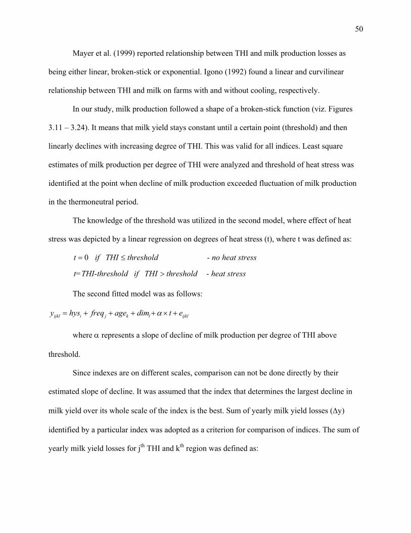
50
Mayer et al. (1999) reported relationship between THI and milk production losses as
being either linear, broken-stick or exponential. Igono (1992) found a linear and curvilinear
relationship between THI and milk on farms with and without cooling, respectively.
In our study, milk production followed a shape of a broken-stick function (viz. Figures
3.11 – 3.24). It means that milk yield stays constant until a certain point (threshold) and then
linearly declines with increasing degree of THI. This was valid for all indices. Least square
estimates of milk production per degree of THI were analyzed and threshold of heat stress was
identified at the point when decline of milk production exceeded fluctuation of milk production
in the thermoneutral period.
The knowledge of the threshold was utilized in the second model, where effect of heat
stress was depicted by a linear regression on degrees of heat stress (t), where t was defined as:
0t if THI threshold - no heat stress
t=THI-threshold if THI threshold - heat stress
= ≤
>
The second fitted model was as follows:
ijkl i j k l ijkly hys freq age dim t eα= + + + + × +
where α represents a slope of decline of milk production per degree of THI above
threshold.
Since indexes are on different scales, comparison can not be done directly by their
estimated slope of decline. It was assumed that the index that determines the largest decline in
milk yield over its whole scale of the index is the best. Sum of yearly milk yield losses (Δy)
identified by a particular index was adopted as a criterion for comparison of indices. The sum of
yearly milk yield losses for jth THI and kth region was defined as:

51
365
1jk jk ij
i
y tα=
Δ = ∑
where αjk is the rate of decline in milk production identified by jth THI in the kth region and
is the sum of degrees of heat stress per year for jth THI and kth region. 365
1ijk
i
t=∑
Results
As shown in Table 3.12, the first model revealed large differences in threshold of heat
stress among indices and between regions, ranging from 68 for THI1 in Athens to 83 for THI4 in
Phoenix. THI1 and THI2 had the lowest and THI3 and THI4 the highest threshold from all
indices in both regions. Thresholds in Athens were on average 3 degrees lower than in Phoenix.
This is probably due to more efficient use of cooling devices in Phoenix.
Indices differed in rate of decline (α) of milk production per degree of THI, ranging from
-0.40 (THI5) to -0.27 (THI2) in Athens and from -0.59 (THI1) to -0.23 (THI6) in Phoenix.
However, because of different scaling (one degree increase in THI doesn’t represent the same
increase in Tdb and RH in all indices) and thresholds, direct comparison of indices using α is not
possible. Table 3.13 presents losses in milk production per year (Δy) detected by THI1-THI7 in
Athens and Phoenix. The largest decline of 127 and 125 kg has been identified by THI2 and
THI1, respectively, in Athens. Those indices are characterized by high Twb and Tdb ratio. In
contrast, the lowest decline in Athens (101 kg) has been detected by THI5, by an index with the
lowest Twb and Tdb ratio. On the other hand, THI5 was the best in Phoenix, with Δy of 168 kg.
The worst indicator of heat stress was THI1 with Δy of 124 kg. This implies that different indices
should be used in humid and different in semi-arid climates. Indices with higher weighting of
humidity are more appropriate for humid climates and vice versa.

52
Disintegrating estimated thresholds of heat stress into Tdb and RH reveals that heat stress
occurs in Athens at temperature ≥ 23°C assuming RH of 75% and in Phoenix at ≥ 30°C and RH
of 25%. Assuming that cows in both regions have on average similar heat tolerance, the fact that
heat stress occurs in Phoenix at much higher temperature, suggests that more effective strategies
are employed to modify the indoor environment of barns in this region.
Conclusions
Temperature humidity indices differ in their ability to detect heat stress. Indices with
larger weight on humidity seem to be more suitable for humid climates. On the other hand, in
climates when humidity doesn’t reach values which could compromise evaporative cooling,
indices placing larger weight on ambient temperature than humidity appear to be more
appropriate indicators of heat stress. Heat stress occurred in the humid climate of Athens at 3
degrees lower THI than in the semi-arid climate of Phoenix. However, severity of heat stress
experienced by a cow over a year was much higher in Phoenix than in Athens. Cautions should
be exercised when comparing results from studies using different THI, since various THI
represent different environmental conditions and therefore direct comparison is not possible.
Literature Cited
Armstrong, D. V. 1994. Heat stress interaction with shade and cooling. J. Dairy Sci. 77:2044-
2050.
Bianca, W. 1962. Relative importance of dry- and wet-bulb temperatures in causing heat stress in
cattle. Nature. 195:251-252.
Bucklin, R. A., J. D. Leary, D. B. McConnell, and E. G. Wilkerson. 2004. Fan and pad
greenhouse evaporative cooling systems. Circular 1135, Department of Agricultural and
53
Biological Engineering, University of Florida.1-7.
Hubbard, K. G. 1994. Spatial variability of daily weather variables in the high plains of the USA.
Agr. Forest Meteorol. 68:29-41.
Huhnke, R. L., L. C. McCowan, L. C. Meraz, S. L. Harp, and M. E. Payton. 2001. Determining
the frequency and duration of elevated temperature-humidity index. ASAE Annual
international meeting, Sacramento, CA, USA.
Igono, M. O., G. Bjotvedt, and H. T. Sanford-Crane. 1992. Environmental profile and critical
temperature effects on milk production of Holstein cows in desert climate. Int. J.
Biometeorol. 36:77-87.
Jensen, M. E., R. D. Burman, and R. G. Allen. 1990. Evapotranspiration and irrigation water
requirements : ASCE – Manuals and Reports on Engineering Practice – No. 70. The
Society, New York, N.Y.
National Research Council. 1971. A guide to environmental research on animals. National
Academy of Sciences, Washington.
SAS. User’s guide. 1999. Statistics, version 8. SAS Inst., Inc. Cary, NC
Thom, E. C. 1959. The discomfort index. Weatherwise. 12:57-60.
Yousef, M. K. 1985. Stress physiology in livestock. CRC Press, Boca Raton, Fla.
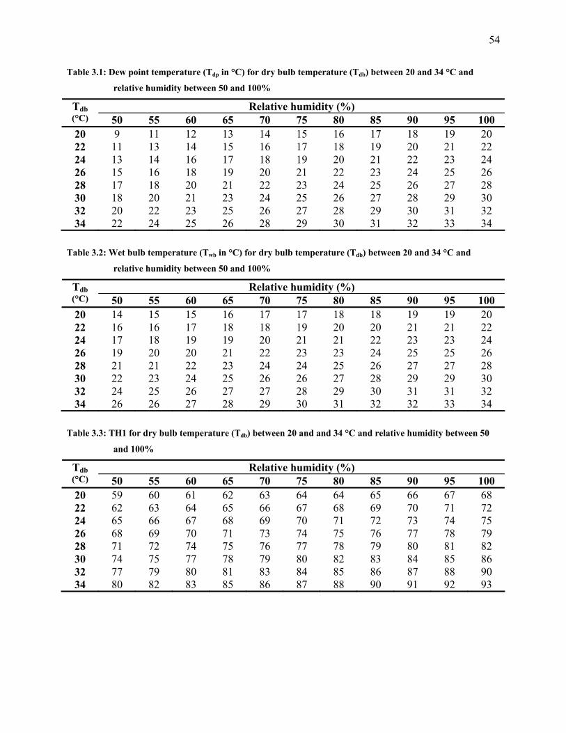
54
Table 3.1: Dew point temperature (Tdp in °C) for dry bulb temperature (Tdb) between 20 and 34 °C and
relative humidity between 50 and 100%
Relative humidity (%) Tdb (°C) 50 55 60 65 70 75 80 85 90 95 100 20 9 11 12 13 14 15 16 17 18 19 20 22 11 13 14 15 16 17 18 19 20 21 22 24 13 14 16 17 18 19 20 21 22 23 24 26 15 16 18 19 20 21 22 23 24 25 26 28 17 18 20 21 22 23 24 25 26 27 28 30 18 20 21 23 24 25 26 27 28 29 30 32 20 22 23 25 26 27 28 29 30 31 32 34 22 24 25 26 28 29 30 31 32 33 34
Table 3.2: Wet bulb temperature (Twb in °C) for dry bulb temperature (Tdb) between 20 and 34 °C and
relative humidity between 50 and 100%
Relative humidity (%) Tdb (°C) 50 55 60 65 70 75 80 85 90 95 100 20 14 15 15 16 17 17 18 18 19 19 20 22 16 16 17 18 18 19 20 20 21 21 22 24 17 18 19 19 20 21 21 22 23 23 24 26 19 20 20 21 22 23 23 24 25 25 26 28 21 21 22 23 24 24 25 26 27 27 28 30 22 23 24 25 26 26 27 28 29 29 30 32 24 25 26 27 27 28 29 30 31 31 32 34 26 26 27 28 29 30 31 32 32 33 34
Table 3.3: TH1 for dry bulb temperature (Tdb) between 20 and and 34 °C and relative humidity between 50
and 100%
Relative humidity (%) Tdb (°C) 50 55 60 65 70 75 80 85 90 95 100 20 59 60 61 62 63 64 64 65 66 67 68 22 62 63 64 65 66 67 68 69 70 71 72 24 65 66 67 68 69 70 71 72 73 74 75 26 68 69 70 71 73 74 75 76 77 78 79 28 71 72 74 75 76 77 78 79 80 81 82 30 74 75 77 78 79 80 82 83 84 85 86 32 77 79 80 81 83 84 85 86 87 88 90 34 80 82 83 85 86 87 88 90 91 92 93

55
Table 3.4: TH2 for dry bulb temperature (Tdb) between 20 and 34 °C and relative humidity between 50 and
100%
Relative humidity (%) Tdb (°C) 50 55 60 65 70 75 80 85 90 95 100 20 61 62 63 63 64 65 65 66 67 67 68 22 64 65 66 67 67 68 69 69 70 71 72 24 67 68 69 70 71 71 72 73 74 74 75 26 71 71 72 73 74 75 76 76 77 78 79 28 74 75 76 77 77 78 79 80 81 82 82 30 77 78 79 80 81 82 83 83 84 85 86 32 80 81 82 83 84 85 86 87 88 89 90 34 83 84 85 87 88 89 90 91 91 92 93
Table 3.5: TH3 for dry bulb temperature (Tdb) between 20 and 34 °C and relative humidity between 50 and
100%
Relative humidity (%) Tdb (°C) 50 55 60 65 70 75 80 85 90 95 100 20 72 72 72 73 73 74 74 75 75 75 76 22 74 75 75 76 76 76 77 77 78 78 79 24 77 77 78 78 79 79 80 80 81 81 82 26 79 80 80 81 82 82 83 83 84 84 84 28 82 83 83 84 84 85 85 86 86 87 87 30 85 85 86 86 87 88 88 89 89 90 90 32 87 88 89 89 90 90 91 91 92 93 93 34 90 91 91 92 93 93 94 94 95 95 96
Table 3.6: TH4 for dry bulb temperature (Tdb) between 20 and 34 °C and relative humidity between 50 and
100%
Relative humidity (%) Tdb (°C) 50 55 60 65 70 75 80 85 90 95 100 20 73 73 74 74 74 75 75 76 76 76 76 22 75 76 76 77 77 78 78 78 79 79 79 24 78 78 79 79 80 80 81 81 81 82 82 26 81 81 82 82 82 83 83 84 84 84 85 28 83 84 84 85 85 86 86 86 87 87 87 30 86 86 87 87 88 88 89 89 89 90 90 32 88 89 90 90 90 91 91 92 92 92 93 34 91 92 92 93 93 94 94 94 95 95 95

56
Table 3.7: TH5 for dry bulb temperature (Tdb) between 20 and 34 °C and relative humidity between 50 and
100%
Relative humidity (%) Tdb (°C) 50 55 60 65 70 75 80 85 90 95 100 20 65 65 65 66 66 66 66 67 67 67 67 22 68 68 69 69 69 70 70 70 71 71 71 24 70 70 71 71 72 72 73 73 74 74 74 26 73 73 74 74 75 76 76 77 77 78 78 28 75 75 76 77 77 78 79 79 80 81 81 30 78 79 79 80 81 82 82 83 84 85 85 32 81 82 83 83 84 85 86 87 88 89 89 34 83 84 85 86 87 88 89 90 91 92 92
Table 3.8: TH6 for dry bulb temperature (Tdb) between 20 and 34 °C and relative humidity between 50 and
100%
Relative humidity (%) Tdb (°C) 50 55 60 65 70 75 80 85 90 95 100 20 65 66 66 66 67 67 68 68 69 69 69 22 68 68 69 69 70 70 71 71 71 72 72 24 70 71 71 72 72 73 73 74 74 75 75 26 73 74 74 75 75 76 76 77 77 78 78 28 76 76 77 77 78 78 79 79 80 80 81 30 78 79 79 80 81 81 82 82 83 83 84 32 81 81 82 83 83 84 85 85 86 86 87 34 83 84 85 85 86 87 87 88 88 89 90
Table 3.9: TH7 for dry bulb temperature (Tdb) between 20 and 34 °C and relative humidity between 50 and
100%
Relative humidity (%) Tdb (°C) 50 55 60 65 70 75 80 85 90 95 100 20 65 65 66 66 66 67 67 67 68 68 68 22 67 68 68 69 69 69 70 70 71 71 71 24 70 70 71 71 72 72 73 73 73 74 74 26 73 73 74 74 74 75 75 76 76 76 77 28 75 76 76 77 77 78 78 78 79 79 79 30 78 78 79 79 80 80 81 81 81 82 82 32 80 81 82 82 82 83 83 84 84 84 85 34 83 84 84 85 85 86 86 86 87 87 87

57
Table 3.10: Descriptive statistics of weather data from Athens and Phoenix
Athens Phoenix Daily minimum Mean SD Min Max Mean SD Min Max
RH (%) 50 17 16 96 19 8 5 48 Tdb (°C) 12 7 -4 23 18 8 3 33 Twb (°C) 11 7 -6 23 12 6 1 23 Tdp (°C) 9 9 -12 22 1 7 -14 18
THI1 52 13 22 73 55 11 33 76 THI2 52 13 23 74 57 12 34 79 THI3 63 11 40 80 68 10 50 87 THI4 65 10 42 81 69 10 50 88 THI5 54 12 28 74 61 10 39 80 THI6 57 11 33 74 62 10 43 80 THI7 57 10 34 73 61 10 42 80
Daily average Mean SD Min Max Mean SD Min Max RH (%) 72 13 39 99 32 13 11 74 Tdb (°C) 17 7 1 29 24 8 9 38 Twb (°C) 14 7 -1 24 15 5 4 24 Tdp (°C) 11 8 -8 23 4 7 -9 20
THI1 58 12 31 76 61 10 42 79 THI2 59 12 31 78 64 11 43 83 THI3 69 10 47 85 75 10 56 91 THI4 70 10 48 86 74 10 56 92 THI5 61 11 36 79 67 9 50 83 THI6 63 10 40 78 68 9 50 85 THI7 62 10 40 78 66 10 48 84
Daily maximum Mean SD Min Max Mean SD Min Max RH (%) 93 8 60 100 50 18 19 100 Tdb (°C) 23 7 6 36 30 8 13 45 Twb (°C) 17 6 3 27 18 5 8 27 Tdp (°C) 14 7 -6 26 8 6 -6 23
THI1 64 11 38 81 68 10 47 86 THI2 66 11 39 85 72 11 49 92 THI3 76 9 53 91 82 9 62 99 THI4 77 9 54 93 81 10 61 98 THI5 69 10 45 85 73 8 57 88 THI6 69 9 47 85 75 9 56 93 THI7 69 10 45 85 73 10 53 90

58
Table 3.11: Descriptive statistics of performance data (1993-2004) from herds nearby Athens and Phoenix
Athens Phoenix Mean SD Min Max Mean SD Min Max
Number of records 110,480 - - - 683,876 - - - Number of cows 12,473 - - - 81,889 - - - Number of herds 61 - - - 53 - - - Number of test days per cow 9 2 1 13 8 2 1 17 Days in milk 174 97 5 365 166 93 5 365 Milk (kg) 28 7 2 59 30 7 2 79 Distance between herd and weather station (km) 32 9 2 51 23 14 10 70
Table 3.12: Threshold of heat stress and rate of decline (α ) of milk production (in kg) due to heat stress for
seven THIs
Athens Phoenix Threshold α (kg) Threshold α (kg)
THI1 68 -0.29 73 -0.59 THI2 69 -0.27 74 -0.26 THI3 78 -0.38 83 -0.29 THI4 79 -0.37 82 -0.28 THI5 72 -0.40 74 -0.31 THI6 72 -0.39 75 -0.23 THI7 71 -0.37 74 -0.28
Table 3.13: Ratio of Twb and Tdb (Twb :Tdb) in THI1-THI7, yearly heat stress degrees and yearly losses (Δy) in
milk production due to heat stress detected by THI1-THI7 in Athens and Phoenix, rank of THI
based on Δy
Athens Phoenix Twb:Tdb Heat street degrees Δy (kg) Rank Heat street degrees Δy (kg) Rank
THI1 5.7 436 -125 2 211 -124 7 THI2 1.9 471 -127 1 536 -142 5 THI3 1.0 302 -113 3 447 -131 6 THI4 1.2 291 -109 4 580 -163 2 THI5 0.3 255 -101 7 542 -168 1 THI6 1.0 264 -104 6 634 -147 4 THI7 1.2 285 -105 5 585 -162 3

Figure 3.1: Average diurnal pattern of January dry bulb temperature (Tdb in °C) and relative humidity (RH in %) in Phoenix and Athens
January
30
61
52
8019
911
3
0
10
20
30
40
50
60
70
80
90
100
0 1 2 3 4 5 6 7 8 9 10 11 12 13 14 15 16 17 18 19 20 21 22 23
hours
RH
(%)
0
5
10
15
20
25
T db
(°C
)
RH PhoenixRH AthensTdb PhoenixTdb Athens
59

Figure 3.2: Average diurnal pattern of June dry bulb temperature (Tdb in °C) and relative humidity (RH in %) in Phoenix and Athens
June
29
13
57
93
26
39
1929
0
10
20
30
40
50
60
70
80
90
100
0 1 2 3 4 5 6 7 8 9 10 11 12 13 14 15 16 17 18 19 20 21 22 23
hours
RH
(%)
0
5
10
15
20
25
30
35
40
45
T (%
)
RH PhoenixRH AthensTdb PhoenixTdb Athens
60
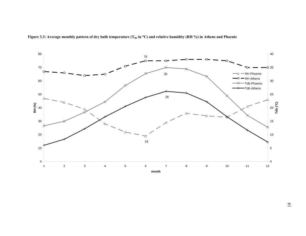
Figure 3.3: Average monthly pattern of dry bulb temperature (Tdb in °C) and relative humidity (RH %) in Athens and Phoenix
19
75
35
26
0
10
20
30
40
50
60
70
80
1 2 3 4 5 6 7 8 9 10 11 12
month
RH
(%)
0
5
10
15
20
25
30
35
40
Tdb
(°C
)
RH PhoenixRH AthensTdb PhoenixTdb Athens
61
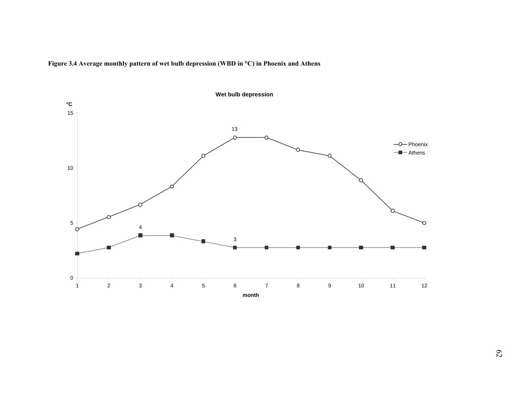
Figure 3.4 Average monthly pattern of wet bulb depression (WBD in °C) in Phoenix and Athens
Wet bulb depression
13
3
4
0
5
10
15
1 2 3 4 5 6 7 8 9 10 11 12
month
°C
PhoenixAthens
62

Figure 3.5: Average June diurnal pattern of temperature humidity indices (THI 1- THI 7) in Phoenix
Phoenix - June
60
70
80
90
100
0 1 2 3 4 5 6 7 8 9 10 11 12 13 14 15 16 17 18 19 20 21 22 23
hour
THI1THI2THI3THI4THI5THI6THI7
63

Figure 3.6: Average June diurnal pattern of seven temperature humidity indices (THI1-THI7) in Athens
Athens - June
60
70
80
90
100
0 1 2 3 4 5 6 7 8 9 10 11 12 13 14 15 16 17 18 19 20 21 22 23
hour
THI1THI2THI3THI4THI5THI6THI7
64

Figure 3.7: Average monthly pattern of THI1- THI7 in Phoenix
Phoenix
4951
55
59
66
71
76 76
72
63
54
48
6365
69
73
80
85
88 88
85
76
67
62
40
50
60
70
80
90
1 2 3 4 5 6 7 8 9 10 11 12
month
THI1THI2THI3THI4THI5THI6THI7
65
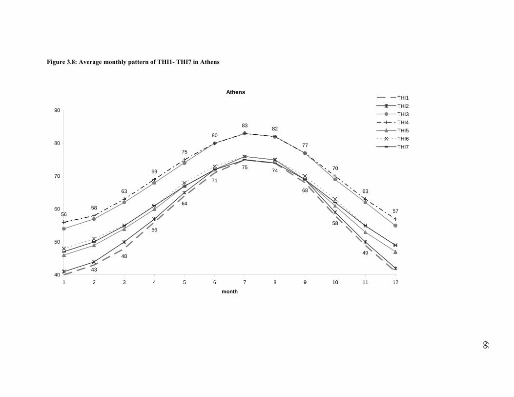
Figure 3.8: Average monthly pattern of THI1- THI7 in Athens
Athens
48
56
64
71
75 74
68
58
49
5658
63
69
75
80
83 82
77
70
63
57
4340
50
60
70
80
90
1 2 3 4 5 6 7 8 9 10 11 12
month
THI1THI2THI3THI4THI5THI6THI7
66

Figure 3.9: Seasonal differences in milk production in herds near Athens and Phoenix
-3
-2
-1
0
1
2
1 2 3 4 5 6 7 8 9 10 11 12
month
milk
(kg)
Athens
Phoenix
67

Figure 3.10: Temperature humidity index (THI5) with (cooled) and without (not cooled) accounting for use of evaporative cooling
THI
58
62
66
72
76
8081
77
69
61
55
62
67
75
71
64
58
49
5453
47
47
52
58
65
71
7473
68
59
52
45
56
5453
59
55
46
61
72
76
44
40
45
50
55
60
65
70
75
80
85
1 2 3 4 5 6 7 8 9 10 11 12
month
Phoenix not cooledPhoenix cooledAthens not cooledAthens cooled
68

Figure 3.11: Least square estimates (x), regression on degrees of THI1 (solid line), a threshold of heat stress and a slope of decline of milk yield in Phoenix
THI1 - Phoenix
73
20
22
24
26
28
30
25 35 45 55 65 75 85 95
THI
milk
(kg)
-0.59
Figure 3.12: Least square estimates (x), regression on degrees of THI1 (solid line), a threshold of heat stress and a slope of decline of milk yield in Athens
THI1 - Athens
68
20
22
24
26
28
30
25 35 45 55 65 75 85 95
THI
milk
(kg) -0.29
Figure 3.13: Least square estimates (x), regression on degrees of THI2 (solid line), a threshold of heat stress and a slope of decline of milk yield in Phoenix
THI2- Phoenix
74
20
22
24
26
28
30
25 35 45 55 65 75 85 95
THI
milk
(kg)
-0.26
Figure 3.14: Least square estimates (x), regression on degrees of THI2 (solid line), a threshold of heat stress and a slope of decline of milk yield in Athens
THI2 - Athens
69
20
22
24
26
28
30
25 35 45 55 65 75 85 95
THI
milk
(kg) -0.27
69

Figure 3.15: Least square estimates (x), regression on degrees of THI3 (solid line), a threshold of heat stress and a slope of decline of milk yield in Phoenix
THI3 - Phoenix
83
20
22
24
26
28
30
25 35 45 55 65 75 85 95
THI
milk
(kg)
-0.29
Figure 3.16: Least square estimates (x), regression on degrees of THI3 (solid line), a threshold of heat stress and a slope of decline of milk yield in Athens
THI3 - Athens
78
20
22
24
26
28
30
25 35 45 55 65 75 85 95
THI
milk
(kg)
-0.38
Figure 3.17: Least square estimates (x), regression on degrees of THI4 (solid line), a threshold of heat stress and a slope of decline of milk yield in Phoenix
THI4 - Phoenix
82
20
22
24
26
28
30
25 35 45 55 65 75 85 95
THI
milk
(kg)
-0.28
Figure 3.18: Least square estimates (x), regression on degrees of THI4 (solid line), a threshold of heat stress and a slope of decline of milk yield in Athens
THI4 - Athens
79
20
22
24
26
28
30
25 35 45 55 65 75 85 95
THI
milk
(kb) -0.37
70
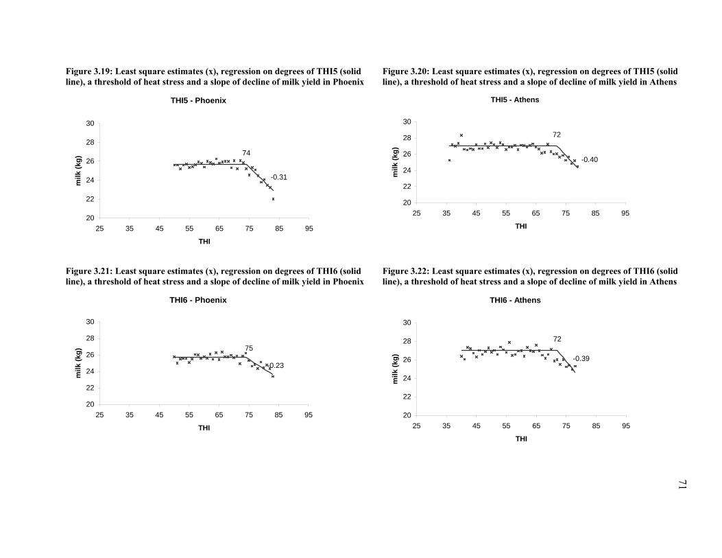
Figure 3.19: Least square estimates (x), regression on degrees of THI5 (solid line), a threshold of heat stress and a slope of decline of milk yield in Phoenix
THI5 - Phoenix
74
20
22
24
26
28
30
25 35 45 55 65 75 85 95
THI
milk
(kg)
-0.31
Figure 3.20: Least square estimates (x), regression on degrees of THI5 (solid line), a threshold of heat stress and a slope of decline of milk yield in Athens
THI5 - Athens
72
20
22
24
26
28
30
25 35 45 55 65 75 85 95
THI
milk
(kg)
-0.40
Figure 3.21: Least square estimates (x), regression on degrees of THI6 (solid line), a threshold of heat stress and a slope of decline of milk yield in Phoenix
THI6 - Phoenix
75
20
22
24
26
28
30
25 35 45 55 65 75 85 95
THI
milk
(kg)
-0.23
Figure 3.22: Least square estimates (x), regression on degrees of THI6 (solid line), a threshold of heat stress and a slope of decline of milk yield in Athens
THI6 - Athens
72
20
22
24
26
28
30
25 35 45 55 65 75 85 95
THI
milk
(kg) -0.39
71

72
Figure 3.24: Least square estimates (x), regression on degrees of THI7 (solid line), a threshold of heat stress and a slope of decline of milk yield in Athens
THI7 - Athens
71
20
22
24
26
28
30
25 35 45 55 65 75 85 95
THI
milk
(kg) -0.37
Figure 3.23: Least square estimates (x), regression on degrees of THI7 (solid line), a threshold of heat stress and a slope of decline of milk yield in Phoenix
THI7 - Phoenix
74
20
22
24
26
28
30
25 35 45 55 65 75 85 95
THI
milk
(kg)
-0.28

73
CHAPTER 4
NATIONAL GENETIC EVALUATION OF MILK YIELD FOR HEAT TOLERANCE
OF UNITED STATES HOLSTEINS
J. Bohmanova, I. Misztal, S. Tsuruta, H.D. Norman, T. J. Lawlor. 2005. Interbull Bulletin. 33:160-162.
(modified)

74
Abstract
The objective of this study was to conduct a national genetic evaluation of milk yield for
heat stress and to identify genetically heat tolerant Holstein bulls. Production data consisted of
57 million test-day records of 7 million primiparous Holstein cows that calved from 1993
through 2004. Hourly temperature and relative humidity records were available from 202 public
weather stations across the United States. The repeatability test-day model included fixed effects
of herd-test date, days in milk class, frequency of milking, age at calving, Based on estimated
heat tolerance PTAs, the 100 most and 100 least heat-tolerant sires were selected. For each of the
200 sires, official U.S. PTAs from February 2006 were obtained. Sires that were the most heat
tolerant transmitted lower milk yields with higher fat and protein contents than did sires that
were the least heat tolerant. Daughters of the most heat tolerant sires had better udder and body
composites, better type, lower dairy form, slightly higher TPI, longer productive life, higher
daughter pregnancy rate, easier calving and better persistency than did daughters of the least heat
tolerant sires. Continued selection for milk yield without consideration of heat tolerance may
result in greater susceptibility to heat stress.
Introduction
Heat stress is an important factor that significantly affects production and reproduction of
dairy cattle in the United States. Estimated total annual economic losses to the dairy industry due
to heat stress range from $897 to $1500 million (St-Pierre et al., 2003). Therefore, genetic
selection for improved heat tolerance could be a cost effective solution of this problem.
Selection on production in an optimal environment results in increased sensitivity in a
harsh environment (van der Waaij, 2004). The long-term selection of U.S. Holstein cattle for
75
milk production was carried out mainly in a temperate climate, and could have lead to an
increase of sensitivity to heat stress over the years.
The level of heat stress can be measured by an animal’s response to climatic conditions.
Climatic conditions can be described by a combination of environmental factors such as air
temperature, solar radiation, relative humidity, and wind speed. However, the majority of these
variables is not recorded in a consistent way and therefore can not be used for a national
evaluation. The temperature humidity index (THI) combines dry bulb temperature and relative
humidity and is a popular choice for large scale studies because both variables are recorded daily
at public weather stations. Meteorological data from weather stations provide an accurate
description of environmental conditions for farms even miles away. However, if cooling devices
are used on the farm, the actual climatic conditions in the barn are different from those at the
weather station. This fact can obscure identification of the real effect of heat stress.
Unfortunately, accounting for the effect of cooling is compromised by a lack of adequate records
on use and efficiency of these heat abatement devices.
More efficient metabolism and consequently lower heat production is one of the main
characteristics of a heat tolerant animal (Lee, 1953). In a harsh environment more resources are
required for fitness and health related traits than in an optimal environment. A heat tolerant cow
which metabolizes nutrients more effectively has more resources for fitness, health, and
reproduction, compared to her heat sensitive contemporaries. On this basis, it can be
hypothesized that a heat tolerant cow is more resistant not only to heat stress but also to other
stressors such as diseases, feed quality and quantity and parasites. In such a heat tolerant cow,
improved fertility and fewer health problems can lead to a longer productive life.

76
Ravagnolo and Misztal (2000) presented a methodology for genetic evaluation of heat
tolerance using test-day milk yield and climatic records from weather stations. The authors
separated predicted transmitting ability into a part describing genetic potential for milk
production in thermoneutral environments (traditional PTA) and a part describing genetic
potential for milk production under thermal conditions (PTA for heat tolerance). When this
approach was applied to the test-day milk yield of Holstein cows in Georgia, a genetic
correlation of -0.35 was found between the traditional and heat tolerance PTAs, and the genetic
variance of heat tolerance PTAs was large at high THI. This indicates a need for a separate
selection in temperate and thermal climates and suggests a potential for genetic selection of milk
yield under these conditions.
The objective of this study was to run a genetic evaluation of milk yield for heat stress at
the national level and to identify genetically heat tolerant Holstein bulls.
Materials and Methods
Data
The U.S. national data set consisted of 57,315,661 first-parity test-day records of
6,906,815 Holsteins that calved from 1993 through 2004. Hourly temperature and relative
humidity records were available from 202 public weather stations across the United States. Herds
were assigned by distance to the nearest weather station.
Hourly THIs were computed from hourly dry bulb temperature (Tdb) expressed in °C and
relative humidity (RH) expressed as a percentage (National Research Council, 1971):
(1.8 32) - [(0.55 - 0.0055 ) (1.8 - 26)]db dbTHI T RH T= × + × × ×
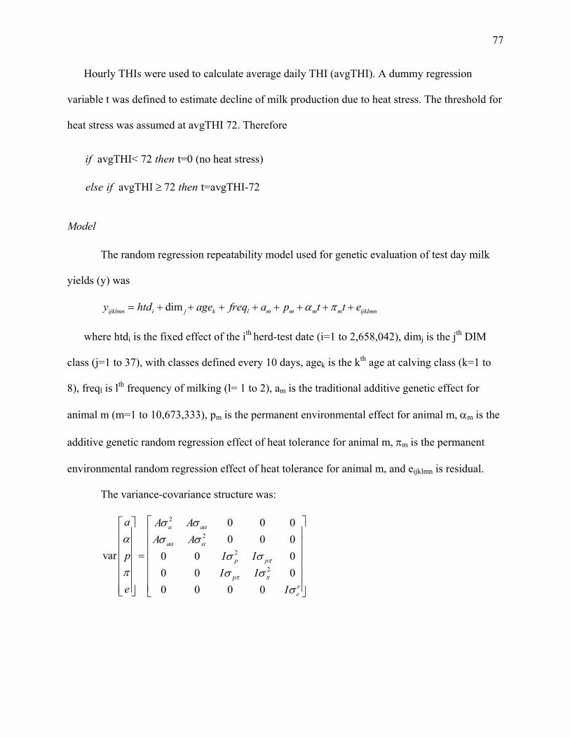
77
Hourly THIs were used to calculate average daily THI (avgTHI). A dummy regression
variable t was defined to estimate decline of milk production due to heat stress. The threshold for
heat stress was assumed at avgTHI 72. Therefore
avgTHI< 72 t=0 (no heat stress)
avgTHI 72 t=avgTHI-72
if then
else if then≥
Model
The random regression repeatability model used for genetic evaluation of test day milk
yields (y) was
dimijklmn i j k l m m m m ijklmny htd age freq a p t t eα π= + + + + + + + +
where htdi is the fixed effect of the ith herd-test date (i=1 to 2,658,042), dimj is the jth DIM
class (j=1 to 37), with classes defined every 10 days, agek is the kth age at calving class (k=1 to
8), freql is lth frequency of milking (l= 1 to 2), am is the traditional additive genetic effect for
animal m (m=1 to 10,673,333), pm is the permanent environmental effect for animal m, αm is the
additive genetic random regression effect of heat tolerance for animal m, πm is the permanent
environmental random regression effect of heat tolerance for animal m, and eijklmn is residual.
The variance-covariance structure was:
2
2
2
2
0 0 00 0 0
var 0 0 00 0 00 0 0 0
a a
a
p p
pee
a A AA A
p I II I
e I
α
α α
π
π π
σ σα σ σ
σ σπ σ σ
σ
⎡ ⎤⎡ ⎤⎢ ⎥⎢ ⎥⎢ ⎥⎢ ⎥⎢ ⎥=⎢ ⎥⎢ ⎥⎢ ⎥⎢ ⎥⎢ ⎥⎢ ⎥⎢ ⎥⎣ ⎦ ⎣ ⎦
78
where A is the relationship matrix, I is the identity matrix, σ2 denotes variance, and σ
covariance. Genetic and environmental parameters were those estimated by Ravagnolo and
Misztal (2000).
Results
The PTAs of 172,411 sires and 10.5 million cows were calculated by BLUP90IOD
(Tsuruta, 2001) in 144 rounds and 8 hours. Heat tolerance PTAs of sires ranged from -0.48 to
0.38 kg milk per THI unit > 72 per day; traditional milk yield PTAs for sires were between -8.9
and 7.9 kg per day.
Based on estimated heat tolerance PTAs, the 100 most and 100 least heat tolerant sires
were selected. For each of the 200 sires, official U.S. PTAs for February 2006 were obtained
(Table 4.1). Sires that were the most heat tolerant transmitted lower milk yields with higher fat
and protein contents than did sires that were the least heat tolerant. Daughters of the most heat
tolerant sires had better udder and body composites, better type, lower dairy form, slightly higher
TPI, longer productive life, higher daughter pregnancy rate and calved easier than did daughters
of the least heat tolerant sires. Daughters of heat tolerant bulls were more persistent in milk, fat
and protein.
Average state PTAs for milk and heat tolerance were calculated as a weighted average
(weighted by number of daughters) of PTAs of bulls having daughters in that state. As given in
Table 4.2, the states in the Southeast and Southwest of the United States were ranked high for
milk but were below average for heat tolerance. Producers in these states are paid based on a
fluid milk pricing system (Bailey and Tozer, 2001). This pricing scheme provides incentives to
select for cows with high milk yield without consideration for solid component content (fat and
protein content). As shown in this study, sires with higher PTAs for milk yield transmit lower

79
heat tolerance to their daughters. It is possible that due to the use of the less heat tolerant sires,
the problem of heat stress in these regions may have been even compounded.
As presented in Figure 4.1, heat tolerance has slightly declined over the years. An
improvement of heat tolerance can be observed after 1995. However, the changes are diminutive.
Similar trend can be seen in daughter pregnancy rate, which declined from 1980 to 1994 and
then increased from 1995 to 1998. The abrupt change in the trend in 1995 can be either attributed
to a smaller number of daughters of sires born after 1995 and consequently lower accuracy of
their proofs, or it could be due to the change in selection strategy. Nonyield traits (productive life
and somatic cell score) were added to the selection index in 1994 (Shook, 2006).
Figure 4.2 shows a trend of 305 day PTAs and test-day PTAs in temperate and heat stress
conditions. The latter PTA was calculated as a sum of heat stress PTA multiplied by the average
number of heat stress degrees per day plus the traditional PTA. The average number of heat
stress degrees per day was set to 1.5, which corresponds to climatic conditions in the southern
United States. The PTA in temperate conditions is simply the traditional PTA. The PTA for 305
day milk yield increased linearly from 1980 to 1998. Predicted transmitted abilities for milk
production in the thermal and heat stress environment were almost identical. Both test-day PTAs
showed a negative trend after 1995. This could have resulted from assumptions imposed by the
model used in this study. The model does not account for differences in persistency, and thus it
could have underestimated younger animals with flatter lactations curves and consequently
created an erroneous negative trend. It will require further investigation to confirm this
hypothesis.

80
Conclusions
Bulls that transmitted high tolerance to heat stress had daughters with lower milk yields,
higher content of milk solids, better udders, longer productive lives, easier calvings, higher
pregnancy rates and better persistency. Continued selection for milk yield without consideration
of heat tolerance may result in greater susceptibility to heat stress.
Acknowledgements
Weather data were available through the Southern Regional Climate Center (Baton
Rouge, LA) as a cooperative effort between Louisiana State University, the National Climatic
Data Center, and the National Weather Service and were provided by J.B. Cole, Animal
Improvement Programs Laboratory, USDA (Beltsville, MD).
References
Bailey, K. and P. Tozer. 2001. An evaluation of federal order reform. J. Dairy Sci. 84:974-986.
Lee, D. H. K. 1953. Manual of field studies on the heat tolerance of domestic animals. Food and
Agriculture Organization of the United Nations, Rome.
National Research Council. 1971. A guide to environmental research on animals. National
Academy of Sciences, Washington.
Ravagnolo O. , I. Misztal and G. Hoogenboom. 2000. Genetic component of heat stress in dairy
cattle, development of heat index function. J. Dairy Sci. 83, 2120-2125
Ravagnolo O. and I. Misztal. 2000. Genetic component of heat stress in dairy cattle, parameter
estimation. J. Dairy Sci. 83, 2126-2130.

81
Shook, G. E. 2006. Major advances in determining appropriate selection goals. J Dairy Sci.
89:1349-1361.
St-Pierre N. R. , B. Cobanov and G. Schnitkey. 2003. Economic losses from heat stress by US
livestock industries. J. Dairy Sci. 86:E52-E77.
Tsuruta S., I. Misztal, and I. Stranden. 2001. Use of the preconditioned conjugate gradient
algorithm as a generic solver for mixed-model equations in animal breeding applications.
J. Anim Sci. 79, 1166-1172.
van der Waaij, E. H. 2004. A resource allocation model describing consequences of artificial
selection under metabolic stress. J. Anim Sci. 82:973-981.
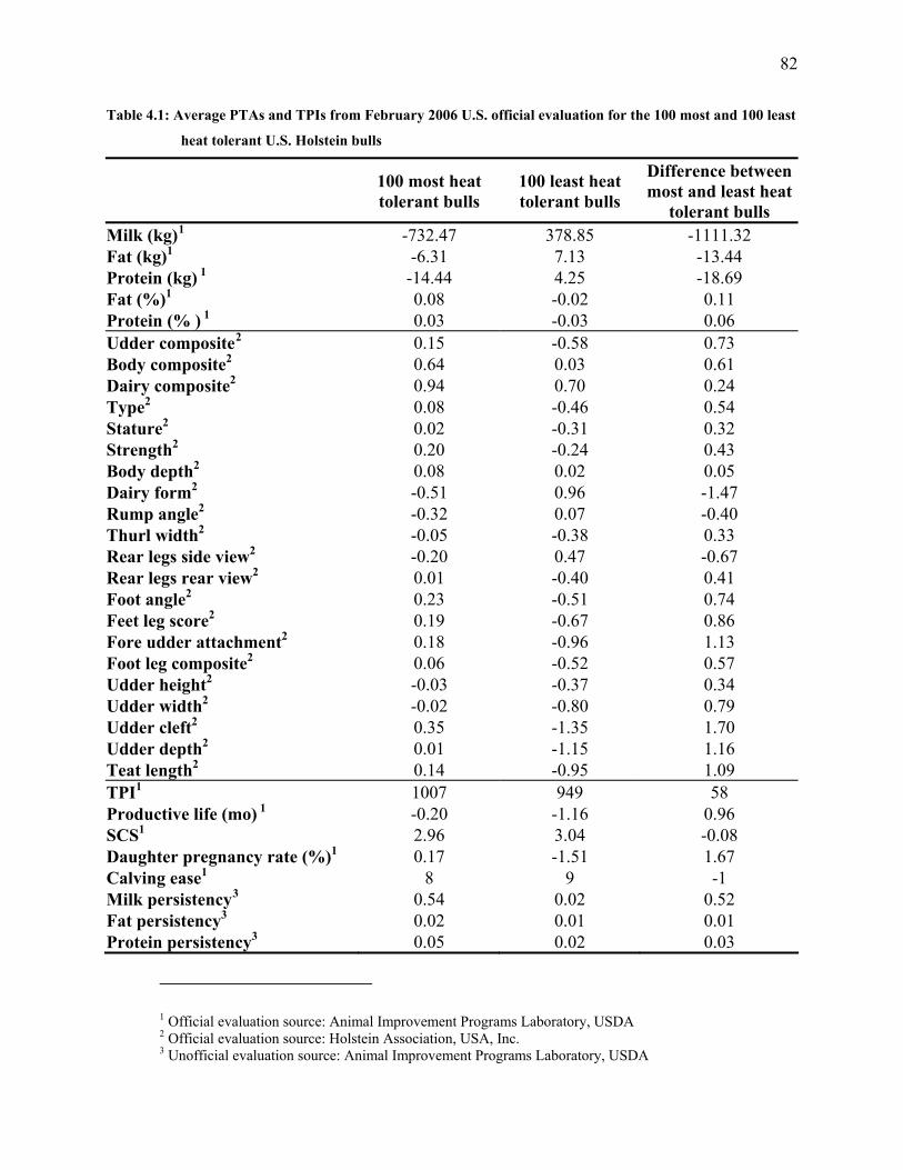
82
Table 4.1: Average PTAs and TPIs from February 2006 U.S. official evaluation for the 100 most and 100 least
heat tolerant U.S. Holstein bulls
100 most heat tolerant bulls
100 least heat tolerant bulls
Difference between most and least heat
tolerant bulls Milk (kg)1 -732.47 378.85 -1111.32 Fat (kg)1 -6.31 7.13 -13.44 Protein (kg) 1 -14.44 4.25 -18.69 Fat (%)1 0.08 -0.02 0.11 Protein (% ) 1 0.03 -0.03 0.06 Udder composite2 0.15 -0.58 0.73 Body composite2 0.64 0.03 0.61 Dairy composite2 0.94 0.70 0.24 Type2 0.08 -0.46 0.54 Stature2 0.02 -0.31 0.32 Strength2 0.20 -0.24 0.43 Body depth2 0.08 0.02 0.05 Dairy form2 -0.51 0.96 -1.47 Rump angle2 -0.32 0.07 -0.40 Thurl width2 -0.05 -0.38 0.33 Rear legs side view2 -0.20 0.47 -0.67 Rear legs rear view2 0.01 -0.40 0.41 Foot angle2 0.23 -0.51 0.74 Feet leg score2 0.19 -0.67 0.86 Fore udder attachment2 0.18 -0.96 1.13 Foot leg composite2 0.06 -0.52 0.57 Udder height2 -0.03 -0.37 0.34 Udder width2 -0.02 -0.80 0.79 Udder cleft2 0.35 -1.35 1.70 Udder depth2 0.01 -1.15 1.16 Teat length2 0.14 -0.95 1.09 TPI1 1007 949 58 Productive life (mo) 1 -0.20 -1.16 0.96 SCS1 2.96 3.04 -0.08 Daughter pregnancy rate (%)1 0.17 -1.51 1.67 Calving ease1 8 9 -1 Milk persistency3 0.54 0.02 0.52 Fat persistency3 0.02 0.01 0.01 Protein persistency3 0.05 0.02 0.03
1 Official evaluation source: Animal Improvement Programs Laboratory, USDA 2 Official evaluation source: Holstein Association, USA, Inc. 3 Unofficial evaluation source: Animal Improvement Programs Laboratory, USDA

83
Table 4.2: Summary of average state milk and heat tolerance PTA, rank of states based on milk and heat
tolerant PTAs and number of cows included in the evaluation per state
State PTA Milk Rank milk PTA heat tolerance Rank heat tolerance No. of cows AZ 5.81 9 -0.08 35 75,598 CA 5.47 25 -0.07 17 1,323,034 CO 6.07 1 -0.07 17 46,175 CT 5.83 7 -0.06 7 36,307 FL 6.05 2 -0.09 39 29,557 GA 5.81 9 -0.07 17 52,789 IA 5.54 21 -0.07 17 183,526 ID 5.37 30 -0.06 7 101,481 IL 5.09 35 -0.05 3 118,272 IN 4.63 39 -0.05 3 90,219 KS 5.32 31 -0.07 17 67,890 KY 5.18 33 -0.06 7 39,211 LA 5.67 14 -0.07 17 21,690 MA 5.49 24 -0.05 3 27,818 MD 4.85 38 -0.03 1 98,078 ME 5.81 9 -0.06 7 32,063 MI 5.52 23 -0.08 35 256,684 MN 5.65 15 -0.07 17 518,473 MO 4.94 37 -0.06 7 63,559 MS 5.83 7 -0.07 17 22,373 NC 5.58 17 -0.07 17 69,746 NE 5.40 28 -0.07 17 56,821 NH 5.84 6 -0.07 17 26,917 NJ 4.97 36 -0.04 2 21,732 NM 5.86 5 -0.07 17 38,634 NY 5.54 21 -0.06 7 644,120 OH 5.40 28 -0.06 7 212,217 OK 5.55 20 -0.06 7 23,676 OR 5.61 16 -0.07 17 81,479 PA 5.24 32 -0.05 3 650,033 SC 5.57 19 -0.07 17 27,561 SD 5.44 27 -0.07 17 34,964 TN 5.58 17 -0.07 17 53,830 TX 5.96 3 -0.08 35 126,891 UT 5.47 25 -0.07 17 64,242 VA 5.78 12 -0.07 17 154,049 VT 5.76 13 -0.06 7 103,706 WA 5.88 4 -0.08 35 134,391 WI 5.18 33 -0.06 7 924,476
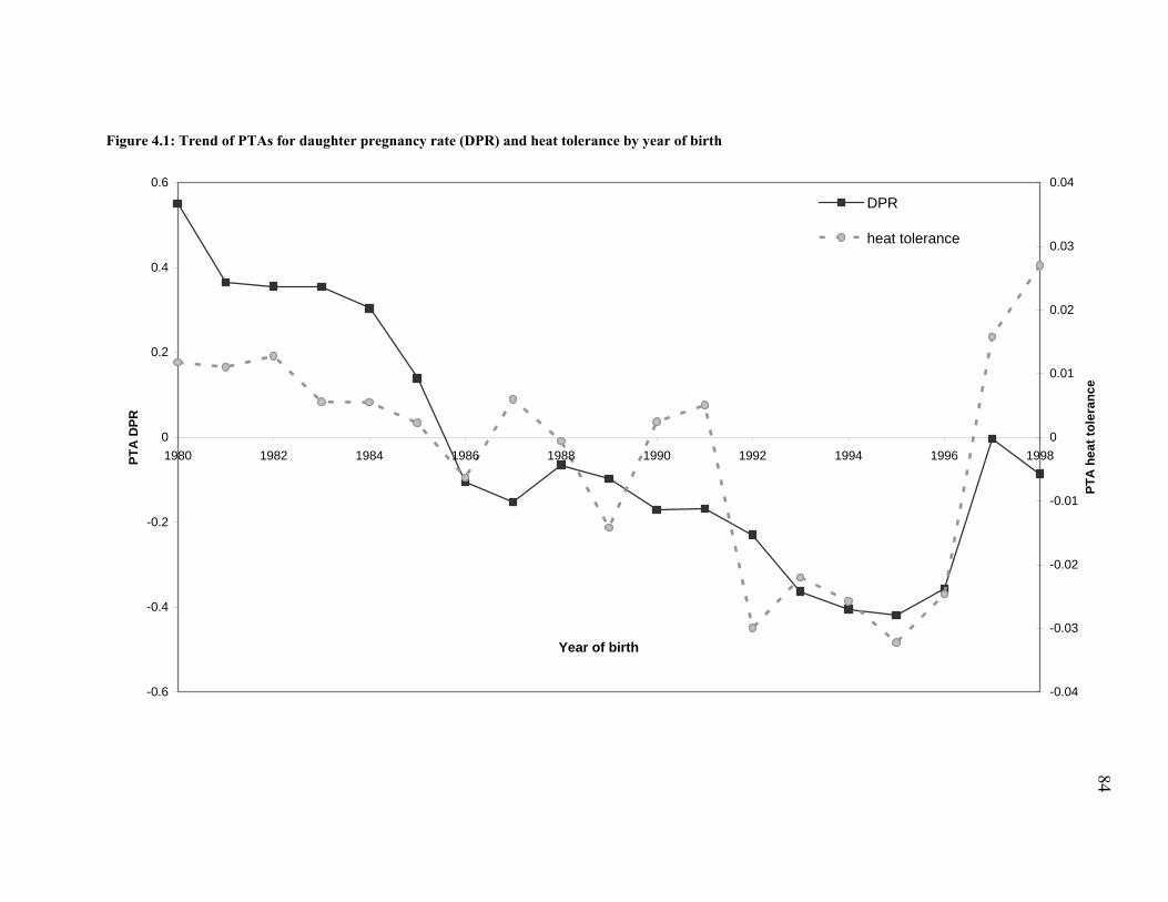
Figure 4.1: Trend of PTAs for daughter pregnancy rate (DPR) and heat tolerance by year of birth
-0.6
-0.4
-0.2
0
0.2
0.4
0.6
1980 1982 1984 1986 1988 1990 1992 1994 1996 1998
Year of birth
PTA
DPR
-0.04
-0.03
-0.02
-0.01
0
0.01
0.02
0.03
0.04
PTA
hea
t tol
eran
ce
DPR
heat tolerance
84

85
-0.5
0
0.5
1
1.5
2
1980 1982 1984 1986 1988 1990 1992 1994 1996 1998
years
test
-day
PTA
-2000
-1500
-1000
-500
0
500
305
day
PTA
TD - thermal (heat stress) conditionsTD - temperate conditions305 day
Figure 4.2: Trend of test-day PTA’s in thermal and temperate conditions and 305 day PTA’s by bull’s birth year
86
CHAPTER 5
HEAT STRESS AS A FACTOR IN GENOTYPE X ENVIRONMENT INTERACTION
IN U.S. HOLSTEINS
1 J. Bohmanova, I. Misztal, S. Tsuruta, H.D. Norman, T. J. Lawlor. Submitted to Journal of Dairy Science
03/15/2006.

87
Abstract
Heat stress was evaluated as a factor in the genotype x environment interaction on milk
production in the United States. The national data set (NA) consisted of 56 million first-parity
test day milk yields on 6 million Holsteins. The Northeastern subset (NE) included 12.5 million
records on 1.3 million cows from eight states, and the Southeastern subset (SE) included 3.5
million records on 0.4 million cows from eleven states. Climatic data were available from 202
public weather stations. Each herd was assigned to the nearest station. Average daily
temperature-humidity index (avgTHI) three days prior to test date was used as an indicator of
heat stress. Two test-day repeatability models were implemented. Effects in both models were
herd-test date, age at calving class, frequency of milking, DIM x season class, additive genetic
(regular breeding value) and permanent environmental effect. The second model additionally
included random regressions on degrees of heat stress (t=max[0,avgTHI-72]) for additive genetic
(breeding value for heat tolerance) and permanent environmental effects. Both models were
fitted with the national and regional data sets. Correlations involved breeding values from SE
and NE for sires with ≥ 100 and ≥ 300 daughters in each region. When heat stress was ignored
(first model) the correlations of regular breeding values between SE and NE for sires with ≥ 100
(≥ 300) daughters were 0.85 (0.87). When heat stress was considered (second model), the
correlation increased by 0.01. The correlations of heat stress breeding values between NE and SE
for sires with ≥ 100 (≥ 300, ≥ 700) daughters were 0.58 (0.72, 0.81). Evaluations for heat
tolerance were similar in cooler and hotter regions for high reliability sires. Heat stress as
modeled explains only a small amount of G x E interaction, partly because test day records
provide only snapshots of heat stress over a hot season.
(Keywords: genotype x environment interaction, reaction norm, heat stress)

88
Introduction
Dairy farming in the US is scattered over a wide range of climatic and topographic
regions, and therefore presence of genotype by environmental (G x E) interaction and thereby re-
ranking of sires in different regions of the United States can be expected. G x E interaction
occurs when genetic correlation of a trait expressed in two different environments is lower than
0.8 (Robertson, 1959). The interaction can be modeled by different statistical models: 1) model
with additional effect of genotype x environment interaction, 2) multitrait model defining records
coming from different environments as a different trait, 3) model with genotype specific random
regression on environmental variables – “reaction norm technique”, where phenotype is
expressed as a function of environmental descriptors (herd production level, herd size,
temperature, humidity, and geographic position).
Large G x E interactions have been reported between countries with different climatic
and production systems, such as New Zealand and United States (Weigel et al., 2001). However,
most of within-country studies did not detect significant interactions. In the study of Carabaño et
al. (1990), genetic correlations of milk production between New York, Wisconsin and California
were all above 0.90 which seems to indicate little evidence for any significant G x E interaction
across those states. Genetic correlations estimated by Rekaya et al. (2003) between five regions
of the United States (Midwest, Northeast, Northwest, Southeast, and Southwest) were all larger
than 0.93. The lowest genetic correlations were between Southeast and Southwest.
In general, differences between regional and national evaluations (r<1.0) can be
explained either by limited accuracies in regional evaluations or due to regional differences in
management and climatic conditions. Zwald et al. (2003) investigated effectiveness of thirteen
genetic, management, and climatic variables in international dairy sire evaluation as indicators of

89
production environments. Authors found lower heritability in herds from cool climates (0.26)
than in herds from hot climates (0.39). Genetic correlations between those two groups were 0.86.
This may suggest that heat stress plays an important role in G x E interaction.
In the study by Norman et al. (2005), correlations between national and regional
evaluations for first parity milk yield ranged between 0.96 (Northeast) and 0.88 (Southeast).
Lowest correlations with Southeast were probably caused by lower number of records in
Southeast and also by much larger impact of heat stress on milk production losses in this specific
region. Regional evaluation may be more or less accurate within a specific region than national
evaluation because on one hand it accounts for the effect of genotype by region interaction but
on the other hand it uses less data.
Ravagnolo and Misztal (2000) proposed a model that accounts for heat stress using
weather data from public weather stations. Their model had two genetic effects per animal, one
corresponding to performance under mild conditions, and one corresponding to a rate of decline
after crossing the threshold of heat stress. The model was first applied to test day milk yield in
Georgia and then Florida (Ravagnolo and Misztal, 2002). The correlation between the two
genetic effects was negative, and the genetic variance due to heat stress was substantial at high
temperature humidity indices. Bohmanova et al. (2005) applied a similar model to the US
national data. Comparisons using sire summaries indicated that heat tolerant sires had lower fluid
milk, higher fertility and productive life, and average TPI. Sires used in the Southeast were
below average for heat tolerance due to the prevalence of fluid milk pricing in the region.
Therefore, problems of heat stress in the Southeast are increasing over time.
The aim of this study was to investigate importance of genotype x environment
interaction in the US Holsteins, to determine if the effect of heat stress can explain a sufficient
90
part of the differences between regional and national genetic evaluations, and to see whether
sires rank the same for heat tolerance in different regions.
Materials and methods
Milk yield data
The data were obtained from AIPL/USDA and included first parity test day (TD) milk
yields of Holsteins calved between 1993 and 2004. The National data set (NA) consisted of
55,494,545 TD records on 5,797,297 cows. The Southeast and the Northeast were defined as in
Norman et al. (2005). The Northeastern data set (NE) included 12,505,982 TD records from CT,
MA, ME, NH, NJ, NY, PA and RI on 1,293,429 cows. The Southeastern data set (SE) included
3,451,223 TD records from AR, AL, FL, GA, LA, MS, NC, OK, SC, TN, TX on 357,130 cows.
All TD records were required to be between 5 and 365 DIM. More detailed description of the
data is given in Table 5.1. As presented in Figure 5.1, the majority of records in SE originated
from Texas (31%), North Carolina (16%), Georgia (12%), Tennessee (11%) and Florida (7%).
The majority of records in NE (85%) originated from New York (44%) and Pennsylvania (41%),
viz. Figure 5.2.
Meteorological data
Hourly meteorological data (temperature and relative humidity) were available from 202
public weather stations across the United States. Temperature humidity index (THI) was
determined from temperature in °C (temp) and relative humidity in % (rh) as follows (National
Research Council, 1971):
[1.8* 32] - [0.55 - 0.0055* )][1.8* - 26]THI temp rh temp= +

91
Hourly THI were rounded to the nearest whole number and averaged over 24 h to obtain
average daily THI. Average daily THI three days prior (avgTHI) to the test date was assigned to
each test day record from the nearest weather station and the threshold of heat stress was set to
avgTHI of 72 for all herds. The choice of a three day lag between weather and yield test day was
based on results from a separate unpublished study, where it was shown that weather data three
days prior to the test date explained more variability than weather data one or two days prior to
the test day or on the test day. Level of heat stress on the farm depends on many factors,
including the use and type of cooling devices. However, this information was not available.
Heat stress degree (t) was used to estimate decline of milk production caused by heat
stress. Heat stress degree was defined as a sum of units of avgTHI above 72. Therefore
avgTHI 72 t=0 (no heat stress)
avgTHI>72 t=avgTHI-72
if then
else if then
≤
Sum of yearly heat stress degrees were calculated for every public weather station and
used as a description of thermal conditions in individual states. As given in Table 5.2, Florida,
Louisiana and Texas are the states with highest heat stress degrees per year in the United States,
with 916, 818 and 761 heat stress degrees per year, respectively. Looking at regions, the
Southeast has on average 596 heat stress degrees per year compared to 88 in the Northeast.
National average is 239.
As shown in Figure 5.3, 10, 7, and 27% of TD records were obtained on days with
thermal stress (avgTHI > 72) in NA, NE and SE. In SE, 14% of TD records were measured on
moderate heat stress days (73 ≤ avgTHI ≤ 76) and 13% on severe heat stress days (avgTHI > 76).
Models

92
Two repeatability models were employed for national and regional genetic evaluations of
test-day milk yields.
Standard model:
ijklmnrijklmnr i j k lm n ry htd age freq dim a p e= + + + + + +
where htdi is the fixed effect of the ith herd-test date, agej is the jth age at calving class (j=1
to 8), freqk is kth frequency of milking (k= 1 to 4), dimlm is the lth DIM class (j=1 to 37), with
classes defined every 10 days, nested within season m (m=1 to 4; December to February, March
to May, June to August, September to November). an is the generic additive genetic effect for
animal n, pr is the permanent environmental effect for animal r, and eijklmnr is residual.
The variance covariance structure was:
2
2
2
0 0var 0 0
0 0
a
r p
s e
a Ap Ie I
σσ
σ
⎡ ⎤⎡ ⎤⎢ ⎥⎢ ⎥ = ⎢ ⎥⎢ ⎥⎢ ⎥⎢ ⎥⎣ ⎦ ⎣ ⎦
where A (n x n) is an additive relationship matrix and Ir is an identity matrix of size r x r
for the permanent environmental effect, Is is an identity matrix of size s x s for the residual (s is
the number of TD records) and σa2=26.45, σp
2=45.98 and σe2=76.49.
Expanded model:
To account for genetic differences in heat tolerance, additional random regressions on
degrees of heat stress were included in the following model:
0 1 0 1 ijklmnrijklmnr i j k lm n n r ry htd age freq dim a a t p p t e= + + + + + × + + × +
where a0n is the additive general genetic effect independent of level of heat stress,
indicating animal’s ability to produce milk in thermoneutral conditions, a1n is the additive genetic
linear random regression coefficient of heat tolerance for animal n, describing animal’s

93
environmental sensitivity to thermal stress, p0r is the permanent environmental general effect
(the basic level), and p1r is the permanent environmental random regression effect (slope) of heat
tolerance for animal r.
The variance covariance structure was:
2
2
2
2
2
0
1
0
1
0 0 0
0 0 0
var 0 0 0
0 0 0
0 0 0 0
a a
a
p p
p
e
a A A
a A A
p I I
p I I
e I
α
α α
π
π π
σ σ
σ σ
σ σ
σ σ
σ
=
⎡ ⎤⎡ ⎤⎢ ⎥⎢ ⎥⎢ ⎥⎢ ⎥⎢ ⎥⎢ ⎥⎢ ⎥⎢ ⎥⎢ ⎥⎢ ⎥⎢ ⎥⎢ ⎥⎣ ⎦ ⎣ ⎦
where σa2=26.74, σaα=-0.89, σα
2=0.16, σp2=46.46, σpπ=-1.17, σπ
2=0.04 and σe2=76.33.
State specific test day breeding values were calculated from the generic (a0) and heat
tolerance (a1) breeding values from the national genetic evaluation as follows:
365
1
365j 0 1 i , ji
a = a + a ( t ) /=
× ∑
where is the average number of heat stress degrees per year in the state j (viz.
Table 5.2).
365
1i , j
i
( t=∑ )
Breeding values were estimated by BLUPIODF90 (Tsuruta et al., 2001), a program that
handles large data sets using iteration on the data technique with a preconditioned conjugate
gradient algorithm.
Results and discussion
As shown in Table 5.3, 636 sires had ≥ 100 daughters in both NE and SE. Those sires had
on average 6,171, 1,413 and 487 daughters in NA, NE and SE, respectively. A second group of
265 sires with ≥ 300 daughters had on average 10,344, 2,310 and 889 daughters in NA, NE and
SE, respectively.

94
Table 5.4 shows correlations of predicted breeding values between national and regional
genetic evaluations for the two sire groups and the two models. For the ≥ 100 (≥ 300) daughters
group using the standard model, the correlations were 0.87 (0.89) in SE and 0.96 (0.97) in NE.
This is similar to correlations of 0.88 and 0.97 obtained by Norman et al. (2005). Correlations
increased with the number of daughters per sire. Correlations between SE and NE increased from
0.87 to 0.89 when the number of daughters increased from 100 to 300; the correlations for the
predicted breeding values are dependent on sire accuracies. When the heat stress effect was
added to the model, those correlations increased by 0.005 in the ≥ 100 daughters group and by
0.009 in the ≥ 300 daughters group. The change was in the expected direction but small,
indicating that adding the heat stress effect in the model does not greatly increase the correlations
between the regular breeding values as expected. Several explanations are possible: a) presence
of G x E interaction due to reasons other than heat stress, b) inadequate model, c) inadequate
weather records, and d) inadequate production data. Freitas et al. (2005) found that response to
heat stress based on test days was about ⅓ that obtained with daily records. This is because the
effect of heat stress between the test days cannot be considered and because only a few
observations per year are used to model variation in cooling over time. Also, the model as used
in this study captures instantaneous but not long-term response to heat stress. Assuming that only
¼ of response to heat stress has been captured in the model with test days, heat stress likely
accounts for a substantial if not the majority of the G x E interaction. To capture more of the heat
stress effect would require more frequent test days.
Table 5.4 also lists the genetic correlations between the NE and SE for the heat stress
breeding value. The correlation increased from 0.58 to 0.72 as the number of daughters per sire
increased from 100 to 300. When sires with ≥ 700 daughters were considered the correlation

95
reached 0.81. Thus the analyses in both regions identified similar heat tolerant sires but only for
sires with high accuracy. Since only a fraction of variability of heat stress is captured with the
test-day data, it requires a large number of records to have a reasonable accuracy. That accuracy
is also a function of the amount of heat stress in a particular region. More heat stress information
per cow is available in data collected in the SE than in the NE, however, the number of cows in
the NE is much larger.
Table 5.5 shows genetic correlations between predicted breeding values in several states
assuming average number of daily heat stress degrees per particular state (Table 5.2) and either
the heat tolerance values as computed in NA or four times larger. The last case assumes that only
¼ response of heat stress has been captured in the model of this paper. When heat tolerant
breeding values are as computed, the correlation between compared states are all > 0.99.
However, with heat stress breeding values four times larger, the correlations between Southeast
and Northeast is < 0.99. Florida, the hottest state in Southeast, has correlation < 0.90 with NE.
This correlation would likely to be much lower if response to heat stress was not masked by
management strategies, such as use of heat abatement devices and timing calving to avoid the
peak of production during the hot season.
Conclusions
Breeding values for heat tolerance calculated in different regions are similar. A national
evaluation for heat stress is possible. However, accuracies of breeding values for heat tolerance
for most bulls are low, and only a small fraction of variability due to heat stress may be
explained by the model used. Therefore only well proven bulls will have reliable evaluations for
heat stress. More information on effects of heat stress can be captured with records tested more
frequently than monthly.

96
Acknowledgments
The authors thank J. B. Cole from Animal Improvement Programs Laboratory, USDA
(Beltsville, MD) for providing the weather data. This study was supported by 58-1265-3-161
grant from AIPL/USDA.

97
References
Bohmanova, J., I. Misztal, S. Tsuruta, H. D. Norman, and T. J. Lawlor. 2005. National genetic
evaluation of milk yield for heat tolerance of United States Holsteins. Interbull Bulletin.
33:160-162.
Carabaño, M. J., K. M. Wade, and L. D. Van Vleck. 1990. Genotype by environment interactions
for milk and fat production across regions of the United States. J. Dairy Sci. 73:173-180.
Freitas, M. S., I. Misztal, J. Bohmanova, J. West. 2006. Utility of on- and off-farm weather
records for studies in genetics of heat tolerance. Liv. Sci. (submitted)
National Research Council. 1971. A guide to environmental research on animals. National
Academy of Sciences, Washington.
Norman, H. D., P. M. VanRaden, R. L. Powell, J. R. Wright, and W. R. Verboort. 2005.
Effectiveness of national and regional sire evaluations in predicting future-daughter milk
yield. J. Dairy Sci. 88:812-826.
Ravagnolo, O. and I. Misztal. 2000. Genetic component of heat stress in dairy cattle, parameter
estimation. J. Dairy Sci. 83:2126-2130.
Ravagnolo, O. and I. Misztal. 2002. Effect of heat stress on nonreturn rate in Holstein cows:
genetic analyses. J. Dairy Sci. 85:3092-3100.
Rekaya, R., K. A. Weigel, and D. Gianola. 2003. Bayesian estimation of parameters of a
structural model for genetic covariances between milk yield in five regions of the United
States. J. Dairy Sci. 86:1837-1844.
98
Robertson, A. 1959. The sampling variance of the genetic correlation coefficient. Biometrics.
15:469-485.
Tsuruta, S., I. Misztal, and I. Stranden. 2001. Use of the preconditioned conjugate gradient
algorithm as a generic solver for mixed-model equations in animal breeding applications.
J. Anim Sci. 79:1166-1172.
Weigel, K. A., R. Rekaya, N. R. Zwald, and W. F. Fikse. 2001. International genetic evaluation
of dairy sires using a multiple-trait model with individual animal performance records. J.
Dairy Sci. 84:2789-2795.
Zwald, N. R., K. A. Weigel, W. F. Fikse, and R. Rekaya. 2003. Identification of factors that
cause genotype by environment interaction between herds of Holstein cattle in seventeen
countries. J. Dairy Sci. 86:1009-1018.

99
Table 5.1: Summary statistics of national and regional data sets
National Northeast Southeast
Number of first parity test day records 55,494,545 12,505,982 3,451,223
Number of cows 5,797,297 1,293,429 357,130
Average milk yield (kg) 29.1 28.3 27.4
Variance of milk yield (kg2) 54.8 53.9 54.0
Average number of primiparous cows per herd 21 16 25
Number of sires 160,058 59,921 28,126

100
Table 5.2: Number of weather stations per state, average (Mean), minimal (Min), maximal (Max) and standard deviation (SD) of yearly heat stress degrees per state
Number of Heat stress degrees per year State weather stations Mean Min Max SD
Region
AL 3 439 346 533 93 Southeast AR 2 562 542 582 28 Southeast AZ 2 701 480 922 312 - CA 8 95 0 333 126 - CO 3 6 0 14 7 - CT 2 96 79 113 24 Northeast DE 1 189 189 189 - - FL 8 916 637 1427 290 Southeast GA 6 452 320 616 112 Southeast IA 4 122 84 166 34 - ID 3 24 3 40 19 - IL 5 152 93 202 43 - IN 4 165 100 295 92 - KS 4 285 193 364 75 - KY 5 216 113 331 101 - LA 4 818 696 938 120 Southeast MA 2 60 30 91 43 Northeast ME 3 81 9 212 114 Northeast MI 7 53 18 99 25 - MN 5 37 9 83 30 - MO 4 289 233 375 63 - MS 3 498 446 555 54 Southeast MT 5 2 0 9 4 - NC 5 265 27 501 172 Southeast ND 3 32 18 44 13 - NE 7 124 13 214 77 - NH 1 32 32 32 - Northeast NJ 2 183 156 210 38 Northeast NM 1 23 23 23 - - NV 4 133 0 520 258 - NY 5 42 16 51 15 Northeast OH 7 89 45 137 32 - OK 2 492 434 551 83 Southeast OR 7 7 0 16 7 - PA 7 111 46 247 73 Northeast RI 1 82 82 82 - Northeast SC 3 443 250 609 181 Southeast SD 4 68 22 97 36 - TN 5 313 64 575 186 Southeast TX 12 761 214 1324 332 Southeast UT 1 47 47 47 - - VA 7 207 40 385 118 - WA 5 5 0 16 7 - WI 5 71 43 105 25 - WV 4 69 12 141 62 - WY 4 2 0 5 2 -
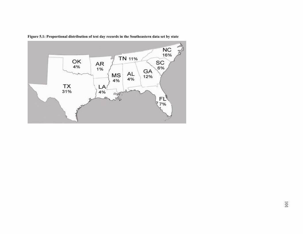
Figure 5.1: Proportional distribution of test day records in the Southeastern data set by state
101

Figure 5.2.Proportional distribution of test day records in the Northeast data set by state
102

Figure 5.3: Frequency of test day records with no heat stress (avgTHI <72), moderate heat stress (73 ≤ avgTHI ≤ 76) and severe heat stress (avgTHI > 76) in
National, Northeast and Southeast data set
90%
7%3%
93%
5%2%
73%
14% 13%
0%
20%
40%
60%
80%
100%
< 72 73 - 76 77- 86
avgTHI
NationalNortheastSouthest
103

104
Table 5.3: Average number of daughters per sire for 636 sires with ≥ 100 daughters and for 265 sires with ≥ 300 daughters in National, Northeast and Southeast
data set.
Mean number of daughters No. sires National Northeast Southeast
≥100 daughters group 636 6,171 1,413 487 ≥300 daughters group 265 10,344 2,310 889

105
Table 5.4: Spearman correlations of sire’s breeding values for heat tolerance additive effect (Corra1_GE), generic additive effect (Corra0_GE) using the Expanded
model and generic additive effect (Corra_G) using the Standard model between Southeast (SE), Northeast (NE) and National (NE) data sets;
differences in correlations of generic additive effects from the Expanded model and the Standard model (Corra0_GE - Corra_G)
Corr a1_GE Corr a0_GE Corr a_G Corr a0_GE – Corr a_G Sires SE x NE SE x NA NE x NA SE x NE SE x NA NE x NA SE x NE SE x NA NE x NA SE x NE SE x NA NE x NA≥ 1007 0.575 0.789 0.774 0.845 0.873 0.962 0.840 0.871 0.961 0.005 0.002 0.001 ≥ 3008 0.715 0.880 0.847 0.874 0.896 0.970 0.864 0.891 0.970 0.009 0.004 0.000
7 Sires with ≥ 100 daughters in both NE and SE
8 Sires with ≥300 daughters in both NE and SE

106
Table 5.5: Spearman correlations of original (as estimated in NA), and altered 9 state specific breeding values (breeding values for heat stress four times larger -
in parentheses)
Southeast Northeast FL GA TX NY
GA 1.00 (0.95) TX 1.00 (0.99) 1.00 (0.98) NY 0.99 (0.86) 1.00 (0.97) 0.99 (0.91) PA 0.99 (0.88) 1.00 (0.98) 0.99 (0.92) 1.00 (1.00)
9 Assumes four times underprediction of heat tolerant breeding values in the model

107
CHAPTER 6
CONCLUSIONS
The results from this study indicate that test-day milk yield records in combination with
meteorological data from public stations provide a valuable source of information for genetic
evaluations of heat tolerance. Heat stress is more effectively alleviated by various modifications
of environment in Phoenix, AZ than in Athens, GA, mainly because the humid climate in Athens
compromises efficiency of evaporative cooling devices. In dry climates ambient temperature
plays more important role than humidity. In humid climates, the amount of moisture in the air is
a more important factor than ambient temperature.
Sires with higher tolerance to heat stress transmit lower milk yields with higher fat and
protein contents. Their daughters have better udders and type, lower dairy form, slightly higher
TPI, longer productive life, higher daughter pregnancy rate, easier calving and better persistency
than daughters of sires that are more sensitive to heat stress. Continued selection for milk yield
without considering heat stress can result in animals with lower heat stress tolerance.
Heat stress explained only a small portion of genotype by environment interaction
between temperate and thermal regions. However, the effect of heat stress could have been much
larger if it was not masked by evaporative cooling. Moreover, the model as used in this study
identifies only the response due to the acute (immediate) and not the chronic (long-term) thermal
stress. Daily milk yield records could be a valuable source of data for more accurate evaluation
of heat stress. Daily records provide enough information which would allow to account for use of
cooling devices (identify threshold of heat stress at a herd x year basis) and identify response to

108
both short and long-term effects of heat stress. Nevertheless, the use of daily records for genetic
evaluation for heat tolerance is currently prevented by limited availability of the records.