Studies of pyridine in water clusters with synchrotron radiation and 3D momentum spectrometry

Benjamin Bolling Thesis submitted for the degree of Bachelor of Science Project duration: 5 months

Supervised by Mathieu Gisselbrecht and Bart Oostenrijk.

Department of Physics Division of Synchrotron Radiation Research

May 2017

1

Studies of pyridine in water clusters with synchrotron radiation and 3D momentum spectrometry

by

Benjamin Bolling

2

3

Acknowledgements I want to direct my gratitude and thanks to my supervisor, Mathieu Gisselbrecht, and my co-supervisor, Bart Oostenrijk. Thank you for your time, effort and the dedication throughout the whole bachelor work, and for always being ready to answer any questions I could have, since I would not have been able to write and complete this thesis without your help and support. I also want to thank my fiancée Helena and my friends David, Saber and Mohammad for supporting and listening to me, and for pushing me in the right direction to be able to finish this work. Thank you all for giving me so much positive energy.

4

5

Contents Chapter 1. Introductory. 7

1.1 Motivation. 7 1.2 Background. 8

1.2.1 Pyridine and pyridine with water clusters 8 1.2.2 Light-matter interactions 8

1.3 The work 11 Chapter 2. Methods. 12

2.1. Experimental setup 12 2.1.1 Mass spectroscopy 12 2.1.2 Momentum spectroscopy 14 2.1.3 RT-plot 15 2.1.4 Coincidence 16

2.2 Data analysis 17 2.2.1 Data structure 17 2.2.2 Metadata 17 2.2.3 GUI structure 18 2.2.4 Filters 19 2.2.5 Recursive filters 20

Chapter 3. Results. 22 3.1 Fragmentation of pyridine molecules. 22

3.1.1 Mass spectrum 22 3.1.2 Correlated mass spectrum 24

3.2 Fragmentation of pyridine and water clusters 27 3.2.1 Mass spectra 27

Files annex 30 Chapter 4. Outlook. 30 Bibliography 31 Appendix A: Calculations. 32

A2: Appendix for calculations for chapter 2. 32 Appendix B: Computer codes for the GUI. 35 Appendix C: Additional plots. 40

6

Acronyms ANACONDA ANAlysis of COiNcidence DAta HCN Hydrogen cyanide GUI Graphical User Interface MCP Multi Channel Plate (detector) m/q Mass over charge PEPIPICO PhotoElectron PhotoIon PhotoIon COincidence RT-plot Radius Time-of-flight TOF Time-Of-Flight

7

Chapter 1. Introductory. 1.1 Motivation. Global warming has increased because of the industrialization, e.g., by the release of greenhouse gases such as carbon dioxide, ammonia, and pyridine [14]. The release of various chemical compounds into the atmosphere can result in them accumulating over time, and become involved in the chemical processes of the atmosphere, e.g. cloud formations and chemistry. Pyridine, which has the chemical formula C5H5N, is produced naturally by belladonna and marshmallow, and in multiple roasting processes, such as during the production of roasted coffee [8], fried bacon [9], and tobacco smoke [10]. The release of pyridine into the atmosphere can be an active element in the cloud chemistry, resulting in the microscopic water droplets to consist of “non-pure” water molecules anymore. By recreating the atmospheric conditions in which the microscopic water droplets are formed during cloud formation, pyridine and pyridine in water clusters are studied and analysed in order to investigate pyridine’s involvement in cloud-like environment. Previous research has been conducted on water clusters using mass spectroscopy, which have shown that protonated water-clusters can consist of anywhere between on to hundreds of water molecules per protonated cluster [4]. With protonated clusters, we mean that one (or more) molecule(s) in the cluster has an excess hydrogen ion (proton) and hence, the cluster becomes positively charged. Pyridine can react in multiple ways, and, for example, act as cloud condensation nucleus [2], which can result in that the water abundance decreases in the atmosphere. Therefore, it is of great importance to study how pyridine and water clusters act together, and if they can be involved as precursors for secondary particle formation. If pyridine is involved in secondary particle formation, and if pyridine accumulates over time, the rate of the secondary particle formation will increase with pyridine’s increased abundance. Hence, precursor molecules are important to study in order to obtain a better understanding of atmospheric chemistry. Another example, which also shows the biological importance of studying pyridine, is that photochemical reactions of pyridine might lead to the formation of HCN (hydrogen cyanide). HCN is a highly reactive and biologically poisonous compound. Therefore, it is important to study if the dissociation of pyridine can result in the formation of e.g. hydrogen cyanide in the environment. In this project, pyridine in water clusters will be analysed by mass spectroscopy fragmentation and 3D momentum spectroscopy. As with most scientific experiments, the analysis requires data treatment before the experimental results can be interpreted. The research group with which this bachelor work is carried out has developed a software for data treatment. The data treatment can be carried out using designated syntaxes in a command-line interface, called ANACONDA2 (analysis of coincidence data). This means that the researcher has to learn such syntax in order to obtain some analysable results, a process which can be time-consuming. To get a faster pace workflow, a GUI (Graphical User Interface) was made. The long term goal is to be able to perform calibration and filtering of the raw data without any coding. The GUI should allow for a smooth and direct visualization of data with elementary data treatment. The results of the pyridine in water clusters analysis using mass spectroscopy fragmentation will show the abundance of the various clusters as a function of the molecular content (number of pyridine resp. water molecules) in order to understand how pyridine interacts with water clusters.

8

1.2 Background. 1.2.1 Pyridine and pyridine with water clusters To understand and interpret the experimental results, the pyridine in water clusters has to be discussed. Pyridine molecules also have to be discussed to provide a reference for pyridine in water clusters. Pyridine belongs to a chemical group called heterocyclic compounds [15]. These molecules have ring-like structures, and consist of two or more different atoms. Pyridine is a flat 6-ring molecule, meaning that it is aromatic. It consists of 5 methylidyne groups (CH) and 1 nitrogen, which has been illustrated in figure 1.1a. A protonated pyridine molecule has also been depicted, which has the chemical name pyridinium. The aromatic, heterocyclic structure results in that the way pyridine reacts strongly depends on the chemical group with which it reacts. For instance, if the reacting chemical group is an electrophile, i.e., a group with a positive terminal (total charge or dipole molecule), electrophilic substitution can take place due to pyridine’s aromatic properties. Electrophilic substitution means that an electron in one of the pi bonds of pyridine performs a nucleophilic attack on the electrophile, i.e. that one of the atoms previously participating in the pi-bond are bond to the electrophile while the other thus becomes positively charged. In figure 1.1b, this has been illustrated as pyridine performs a nucleophilic attack on an electrophile E. One question that could be addressed is how pyridine molecules arrange themselves with water clusters, as illustrated in figure 1.2. In figure 1.2, we have two possible pyridine-water interactions. Either, pyridine molecules stick to a water cluster’s surface (I), or gets embedded within the water cluster (II). 1.2.2 Light-matter interactions Light-matter interaction can be divided into two steps: Excitation/ionization and dissociation/fragmentation (see figure 1.3). The excitation means that the molecular energy state is in a higher energy state than the ground state, while ionization means that the light energy kicks out an electron [12]. In this work, the excitation is completely absent and is hence not treated here. The ionization is most likely to occur for the 1s core electron of the carbon atom (C1s) or the oxygen atom (O1s), due to the high energy of the photon. This leaves a hole in the core shell, which is instantly filled with an electron from an outer shell. Since this results in an atom with a high excess internal energy, it will decay either by kicking out a second electron (Auger decay) or by the emission of a photon (fluorescence).

Figure 1.2: Pyridine stick on the surface of the water clusters (I) and pyridine embedded within water clusters (II).

Figure 1.1. a) Molecular structure of pyridine (A) and pyridinium (B). b) Electrophilic substitution of pyridine with an electrophile E.

1

2

3

4

5

6 A B

a)

b)

9

Auger decay is most probable for low-Z elements (Z< 40) [13]. Hence, the resulting atom is doubly charged. In the case of an atom within a molecule, intra-molecular charge migration occurs with a reaction rate due to and depending on the value of the Coulomb repulsion, which can lead to molecular dissociation. Molecular dissociation can also occur for singly ionized/charged molecules, i.e., without the emission of an Auger electron. This can result in a singly charged fragment and a single or multiple uncharged fragments, or multiple charged fragments (e.g. if the uncharged fragment dissociates into two oppositely charged fragments which would sum up to zero charge).

Using synchrotron radiation as light source, it is possible to have element specific ionization, since the atomic cross-section describes the probability of the photons interacting with the atom and depends on the photon energy [12]. In figure 1.4, the cross-sections of three atomic species (the ones which are included within the clusters), i.e. carbon, nitrogen and oxygen, are plotted against photon energy.

As seen in figure 1.4, the cross section is essentially the same for all atoms at low photon energy (<100 eV), and hence, the ionization cannot be selective. Above the 1s-shell edge, the strong increase of the cross section of an atomic specie allows for ionization of a specific element.

Figure 1.3: Pyridine breakup due to the photochemical reaction, which in this case results mainly in two charged fragments due to the high energy of the photons. Note that only the charged fragments can be detected since only charged fragments can be accelerated with electromagnetic waves.

Figure 1.4: The atomic cross-sections for light interactions with carbon, nitrogen and oxygen.X-ray Data Booklet [3].

10

The possibility to ionize a specific atom can be used to localize the charges (after Auger decay) and investigate how they spread due the strongly Coulomb-repulsed forces, as illustrated in figure 1.5, when one of the carbon atoms gets C1s-ionized.

For sake of simplicity we assume that a single charge migration has happened. In reality, multiple charge migrations can happen in order for the intra-molecular charge separation to be as large as possible. Note that the localization/delocalization of the molecular orbitals plays here a major role. If the repulsion is stronger than the bond strengths, the molecule will break apart and dissociate. The fragmentation (dissociation) can result in two (or more) fragments moving away from one another, thus, each with a momentum larger than zero. Summing up the individual fragments’ momentum results in the total momentum, which has to be equal to 𝑝", which was the original total momentum of the molecule before its fragmentation:

𝑝#$# = 𝑝&&

= 𝑝" ≥ 0

with 𝑝& being the momentum of fragment 𝑛. In general, the analysis of fragmentation mechanism requires the determination of momenta of particles, determine the kinematic of the reaction. For practical reasons, scientists study dissociations which can result in a 2-body- or a 3-body breakup. We can now discuss about which photochemical reactions can occur with clusters, which incorporates different molecules (Water and Pyridine). After light-matter interaction, doubly charged originating arising from either a Carbon atom or an Oxygen atom will migrate due to Coulombic forces, leading to fragmentation of the cluster. The resulting dynamic is a complex image, since both ultrafast hydrogen-motion and heterogeneous intra/inter-molecular forces will affect charge motion and bond breaking. Furthermore, as we can see in figure 1.2, the inter-molecular arrangements of the molecules within the cluster may determine the dynamic. On the one hand, when water molecules surround the pyridine molecules, pyridine fragmentation after C-edge ionization may be hindered by other molecules. On the other hand, when the pyridine molecules stick to the surface of water cluster, fragmentation after O-edge ionization may release intact pyridine molecules. These different fragmentation processes could have particular kinematics of reaction and can be measured with 3D momentum imaging technique.

Figure 1.5: Single charge migration in a pyridine molecule if a carbon atom is doubly ionized. The two, singly-charged carbons (encircled in red) are strongly repulsed by Coulombic forces. The charge migration depicted is an electron moving from the previous double-covalent bond into the doubly ionized carbon, marked by the red arrow.

11

1.3 The work Experiments carried out with mass spectroscopy fragmentation are conventionally used to measure the time of flight in order to obtain the chemical composition of a sample in the form of a mass spectra. The experimental setup developed in the group is a more advanced mass spectrometer, which allow also to measure the 3D momentum of charged particles in coincidence. The power of this experimental method is to correlate particles masses and momenta. High order coincidences can be analysed and thus provide a full information about the dynamics of the molecular dissociation into fragments. This will be addressed in the method section. Experiments which involves clusters means that a lot of data has to be treated. The group has developed a software, ANACONDA2 (analysis of coincidence data) based on MATLAB with which experimental data can be treated. The GUI was developed in order to simplify and make data analysis with ANACONDA2 more efficient. Previously, it was necessary to write scripts together with nested and recursive functions in order to do the data treatment, since it was built as a command-line interface. The GUI includes most of its built-in functionalities so that data treatment can be carried out visually in an easy and smooth way. The GUI also gives the possibility to carry out data treatments for multiple data files at the same time. To achieve this, the GUI had to be created with many algorithms together, combining multiple, multi-layer nested and recursive functions. The GUI also includes a filter module, designed as a tree, which had to be done using a JAVA-component in MATLAB. The scope of the filter is to only provide the data of interest after or during data treatment, while ‘filtering out’ (or getting rid of) data which is not in the scope of interest for the data analysis, as it could interfere with the data of interest. This was not an easy task since the tree JAVA-component did not have any proper documentation, and similar functions were not found within MATLAB. This meant that the filter tree had to be developed empirically, with trials and errors. The filter module allows for adding, copying, editing, removing and combining filters. The filters will be discussed in chapter 2.2.4, where details will also be revealed about how it works and why it is such a powerful tool in data treatment. The GUI was tested by using a set of data obtained from a 3D momentum spectrometer experiment carried out on pyridine and pyridine in water clusters. The experiment itself was carried out at MAXLAB in Lund, Sweden, 2012. In the following, the method section will describe the physics behind the 3D momentum spectrometer, the data structure and the GUI. In the result section, the fragmentation results of pyridine are presented using the GUI for the data analysis. The results are briefly analysed, interpreted and discussed. The last chapter provides conclusion, concerning the functionality of the GUI and the experimental results.

12

Chapter 2. Methods. We studied two type of samples: Pyridine molecules and pyridine and water mixed clusters. The pyridine samples were fragmented by synchrotron light, i.e., photons. As the sample breaks apart, the fragments will be emitted as particles that are either charged (positively or negatively), or neutral. The charged particles are collected by a 3D momentum spectrometer. 2.1. Experimental setup The spectrometer to facilitate this study is described below.

The experimental setup is schematically represented in figure 2.1 [1]. The experiment is setup in a vacuum chamber to prevent emitted particles to interact with residual gas. The principle of the spectrometer is as follow. A static electric field is applied to region I, where the electric field exerts a force in the longitudinal axis (z) on the charged particles. This causes them to accelerate along this axis, with positively charged particles accelerating against the detector screen and negatively charged particles accelerating away from the detector screen. The positively charged particles entered after region I into a drift tube (i.e. free from electro-magnetic fields), region II, where no forces affects the ions. At the end of region II, a position sensitive detector collects the charged ions. The detector is a Micro Channel Plate detector, which amplifies the signal, and a commercial Delay Line Anode from Roentdek GmbH, which collects a hit as two spatial coordinates gives them a timestamp of ‘when’ the particle hit the detector screen [5]. The time it takes for an ion with mass 𝑚 and charge 𝑞 from a source point, in 𝑧", to a detector, in 𝑧-, is the underlying basis of mass spectroscope. 2.1.1 Mass spectroscopy We will now derive the principle of classical motion of ions in a one field spectrometer.

- Region I: Acceleration region, where an electric field 𝐸 is present and accelerates the particle with charge 𝑞.

- Region II: Drift region, where no electric field exists. No forces act on the particle.

Figure 2.1: Principle of the experiment using a 3D momentum spectrometer for charged particles. Region I is an extraction and acceleration region with an electric field and region II is a drift tube region with no electric field.

hv

13

In region I, the charged particle is accelerated over 𝑧/ − 𝑧" =1- unit lengths with a constant electric

field, 𝐸. The acceleration, 𝑎, can be determined by the force acting on the particle:

𝑞𝐸 = 𝑚𝑎 2.1

where 𝑞 is the charge of the particle, 𝑚 is the particle mass. The initial velocity of the particle can be divided into two parts: one along the 𝑧-axis, which is the direction of the electric field, and the other part called the radial direction 𝑅 = 𝑥- + 𝑦-. Hence, the initial velocity of the fragment is:

𝑣"- = 𝑣";- + 𝑣"<- + 𝑣"=- = 𝑣";- + 𝑣">- 2.2

where 𝑣>" = 𝑣<"- + 𝑣="- is the radial velocity of the fragments.

The motion of a particle along the z-axis is described by 𝑑𝑝;𝑑𝑡 = 𝑞𝐸 ↔ 𝑑𝑝; = 𝑞𝐸𝑑𝑡 2.3

where the momentum is 𝑝; = 𝑚𝑣;. since only the momentum in the longitudinal (𝑧-) direction is affected, as 𝐸 = 𝐸;. This equation can be integrated:

𝑑𝑝; = 𝑞𝐸𝑑𝑡 = 𝑞𝐸 𝑑𝑡 2.4

A detailed derivation for the time-of-flight (TOF) in regions I and II in figure 2.1 is made in appendix A2, and results in that the time-of-flight in region I, 𝑡D, and region II, 𝑡DD, becomes

𝑡D = −𝑚𝑣";𝑞𝐸 +

𝑚𝑣";𝑞𝐸

-+𝑚𝑑𝑞𝐸 =

𝑚-𝑣";- + 𝑞𝐸𝑚𝑑 −𝑚𝑣";𝑞𝐸 2.5

𝑡DD =𝐿

𝑣"; + ∆𝑣D=

𝐿𝑣"; + 𝑎 ∙ 𝑡D

2.6

where 𝑑 is the length of region I and 𝐿 is the length of region II. The TOF (time-of-flight) depends on the mass and the charge of the particle, and hence, a TOF-spectra be translated to a ‘mass-over-charge’ (m/q) spectra for simpler identification of the molecular fragments. The mass over charge can hence be determined for the detected particles by using mass spectroscopy, and can be calculated from the TOF since

𝑇𝑂𝐹 = 𝑡D + 𝑡DD 2.7

After some simplification and approximating that 𝑣"; = 0 (since ∆𝑣D ≫ 𝑣";), we find that

𝑇𝑂𝐹 ≈𝑚𝑞𝐸

𝑑 +𝐿𝑑. 2.8

This (eq. 2.8) can be rewritten as 𝑚𝑞 ≈

1𝐾RST

𝑇𝑂𝐹- 2.9

where 𝐾RST is an arbitrary constant which can be defined by the experimental setup (see appendix A2.3 for the full mathematical derivation from eq. 2.7 to eq. 2.9). This implies that a particle’s mass and charge define its flight time, and vice versa, that only by measuring the TOF, the particle’s mass over charge can be found and plotted as a 1-dimensional histogram. This histogram is called a mass-spectra, since the peaks define the intensity (abundance) of the different particles and is the goal of mass spectroscopy.

14

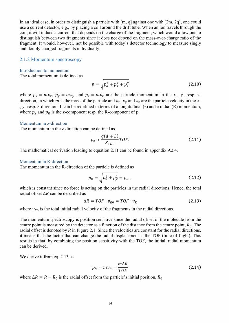
In an ideal case, in order to distinguish a particle with [m, q] against one with [2m, 2q], one could use a current detector, e.g., by placing a coil around the drift tube. When an ion travels through the coil, it will induce a current that depends on the charge of the fragment, which would allow one to distinguish between two fragments since it does not depend on the mass-over-charge ratio of the fragment. It would, however, not be possible with today’s detector technology to measure singly and doubly charged fragments individually. 2.1.2 Momentum spectroscopy Introduction to momentum The total momentum is defined as

𝑝 = 𝑝<- + 𝑝=- + 𝑝;- 2.10

where 𝑝< = 𝑚𝑣<, 𝑝= = 𝑚𝑣= and 𝑝; = 𝑚𝑣; are the particle momentum in the x-, y- resp. z-direction, in which 𝑚 is the mass of the particle and 𝑣<, 𝑣= and 𝑣; are the particle velocity in the 𝑥-, 𝑦- resp. 𝑧-direction. It can be redefined in terms of a longitudinal (z) and a radial (R) momentum, where 𝑝; and 𝑝> is the z-component resp. the R-component of p. Momentum in z-direction The momentum in the z-direction can be defined as

𝑝; ≈𝑞 𝑑 + 𝐿𝐾RST

𝑇𝑂𝐹. 2.11

The mathematical derivation leading to equation 2.11 can be found in appendix A2.4. Momentum in R-direction The momentum in the R-direction of the particle is defined as

𝑝> = 𝑝<- + 𝑝=- = 𝑝>", 2.12

which is constant since no force is acting on the particles in the radial directions. Hence, the total radial offset ∆𝑅 can be described as

∆𝑅 = 𝑇𝑂𝐹 ∙ 𝑣>" = 𝑇𝑂𝐹 ∙ 𝑣> 2.13

where 𝑣>" is the total initial radial velocity of the fragments in the radial directions. The momentum spectroscopy is position sensitive since the radial offset of the molecule from the centre point is measured by the detector as a function of the distance from the centre point, 𝑅". The radial offset is denoted by 𝑅 in Figure 2.1. Since the velocities are constant for the radial directions, it means that the factor that can change the radial displacement is the TOF (time-of-flight). This results in that, by combining the position sensitivity with the TOF, the initial, radial momentum can be derived. We derive it from eq. 2.13 as

𝑝> = 𝑚𝑣> =𝑚∆𝑅𝑇𝑂𝐹 2.14

where ∆𝑅 = 𝑅 − 𝑅" is the radial offset from the particle’s initial position, 𝑅".

15

2.1.3 RT-plot In order to get information about the initial radial momentum of the fragment, one can investigate a RT-plot (Radius Time-of-flight) for the created fragment. The RT-plot gives information about the initial radial momentum and hence about the fragmentation process itself and the initial sample composition. We can now state that p> is reflected on 𝑅 and that p; is reflected on ∆𝑇𝑂𝐹, and that there is a correlation between 𝑅 and ∆𝑇𝑂𝐹. Since p is constant for many reactions, including the photochemical reaction used in this experiment for a constant photon energy, we can expect to see ‘half-rings’, as in Figure 2.2. Figure 2.2 shows how the initial momentum of the fragment determines the hit position on the detector, where a is the hit region of the first fragments which had a momentum vector 𝑝X,Y (directed slightly towards the detector), b is the hit region where fragments had a momentum vector 𝑝X,Z (directed slightly perpendicularly towards the detector, i.e. high initial radial momentum) hit the detector and c is the hit region where fragments had a momentum vector 𝑝X,[ (directed away from the detector). Assuming that the initial kinetic energy of all fragments are (approximately) the same (with some uncertainty ∆𝐸\,X&X#XY]), means that

E_,`a`b`cdecfb`gdh/ = E_,`a`b`cd

ecfb`gdh-. 2.15

The approximation in eq. 2.15 is fairly good as we would otherwise not observe the half-ring in Figure 2.2. We now compare two particles which have different masses but same m/q ratio. For simplicity reasons, we define the mass of particle 2 to be twice as large as the mass of particle 1, i.e., 2𝑚/ = 𝑚-. We also define the charge of particle 2 to be twice as large as the charge of particle 1, i.e., 2𝑞/ = 𝑞-. This means that both particles have the same m/q ratio. Using the classical mechanics definition for a particle’s kinetic energy

𝐸 = 0.5𝑚𝑣- 2.16 for eq. 2.15, we find that (see appendix A2.5 for the full derivation)

v/,`a`b`cd- = 2v-,`a`b`cd- . 2.17

The TOF is therefore related to the particle momentum in the longitudinal direction as

TOF ≈𝑚𝑧#$#𝑝;,#$#

. 2.18

The derivation from eq. 2.17 resulting in eq. 2.18 has been made in appendix A2.6.

Figure 2.2: Detector hit positions a, b and c, depending on the initial momentum vector p of the fragment (F).

d

16

Equation 2.18 states that the particle with the highest, longitudinal momentum pX,; will reach the detector first. Since TOF depends on the initial momentum in the longitudinal direction, so does the radial hit position of the particle on the detector screen. If the initial longitudinal velocity is high, the initial radial velocity will be low. This results in that ‘cd’ decreases while ‘ab’ increases in Figure 2.2, and shows the dependency of the radius R on the TOF. Since the initial velocity of particles with larger mass have a lower initial velocity, doubly charged species (such as particle 2 previously discussed) should be identifiable in the R-TOF spectra as a smaller lobe sitting ‘within’ the larger lobe of the singly charged species (such as particles 1 and 2, which have the same m/q). The lobe is defined as a unit circle (eq. 2.19 for a circle with radius R) as described in eq. 2.20:

𝑅 = 𝑥- + 𝑦- 2.19

𝐸\ ∝ 𝑣X,;- + 𝑣X,>- 2.20

where 𝑣X,; is the initial velocity of the particle in the 𝑧-direction and 𝑣X,> is the initial velocity of the particle in the 𝑅-direction (of which 𝑧 and 𝑅 were defined by figures 2.1 and 2.2). 2.1.4 Coincidence When the synchrotron radiation interacts with the sample, many different particles can be created from one reaction. In order to detect particles arising from the same ionization events, coincident detection of particles is necessary. The scheme for measuring particle in coincidence is illustrated in Figure 2.3. Once an electron hits the detector it triggers/starts the acquisition system. An acquisition window of a few microseconds (10-50 µs) is open to acquire hits coming from the ion detector. The window is defined by the user directly at the machine, and is typically prepared by some necessary calculations depending on the experimental setup (electric field strength, region lengths, etc.) and what fragments are expected. The window can then be defined by opening resp. closing it when the lightest resp. the heaviest fragment are expected to arrive at the detector. The data acquired while the window was open are then stored. Each cycle of acquisition will then be considered as an event where the hit multiplicity defines the degree of coincidence. Single coincidence is referred to as one hit during one event, double coincidence being two hits during one event etc.

Figure 2.3: A fragmentation process, releasing one or more electrons, of which if one (or more) hits the trigger start. This activates a timer, which for a set data acquisition ‘window’ keeps the data. The window typically opens up 5 µs after the start trigger is activated and remains open for typically 20 µs, marked as a green region in the timer above. When the window is open, data is allowed through from the detector to a recorder. Elsewise, no data is allowed through (marked as the red region).

17

2.2 Data analysis Data from experiments are in raw format, which means that the events and their hits have been collected as a data array for each detector. If many fragments are registered as hits, there will be a lot of data since each hit is stored as data. 2.2.1 Data structure The resulting data from a 3D momentum spectrometer is a multidimensional data array with hits and events conditions.

As illustrated previously in Figure 2.3, hits are collected during a detection window and attributed to different events, i.e., the different detection windows. The experimental data are structured as illustrated in Figure 2.4, where it can be observed that each stored hit with its recorded data is attributed to the different events. For example, all events have a number of hits assigned to them (0, 1, 2, …), which all have different masses. The hits that belong to the event have their masses summed up to result in the total mass of the event. The mass of the event is equal to the mother nuclei if all fragments from the event are detected and stored. If the corresponding energies are measured as well, then the event is said to be kinematically complete. 2.2.2Metadata Each experiment’s data has so called metadata connected to it. The metadata is defined for each experiment and stores additional parameters beyond the data itself, such as spectrometer, detector and calibration parameters.

Figure 2.4: Experimental data structure for an N-dimensional spectrometer experiment (where the ‘data’ of each hit number has N dimensions) with, in this illustration, 2 detectors but can be extended to any number of detectors. In the illustration, 5 events have been recorded (denoted as e1 - e5 for the hit section). NaN is an abbreviation for ‘Not a Number’, which means that during the event, no hits were detected.

18

2.2.3GUIstructure The treatment of data can be a time-consuming process, especially if each experiment is treated with a command-line interface. The research group has previously developed a computational method, ANACONDA2, which allows for the experimental data to be treated and visualized. This is done in MATLAB by specified commands, i.e. syntaxes, executed in specific orders. With the GUI, the MATLAB commands are not needed in the same scale as previously for the data treatment, since the GUI enables the researcher to carry out most of the (and the more common) data treatment graphically. The visual result of the GUI can be seen in Figure 2.5, where we show the interfaces for loading multiples experimental files, the generation of filters using an intuitive tree representation based on the java plug-in*, and the (1D, 2D) plotting possibilities. The calibration interface still has to be done, but can be incorporated into the GUI in the near future.

The GUI was ‘hard-coded’ using the in-built UIcontrol system of MATLAB, with which the interface dynamically evolves while the data treatment is progressing without messiness. *Tree Controls for User Interfaces, Robyn Jackey, MathWorks File Exchange.

Figure 2.6: The visual look for the GUI. The loading, filtering and plotting parts are all based on dynamical MATLAB-functions.

19

The structure of the GUI in the ‘hard-code’ level allowed us to structure and design it in a way that allows new functionalities to be added to the kernel ANACONDA2 without the need to update, or restructure, the GUI. Efforts have been made in order to allow data treatment to be done through the GUI automatically, allowing users without any prior knowledge of how the data treatment is made to carry out the data treatment. Here, object programming with proper hierarchy was essential. Recursive and nested algorithms were written, and some parts of the kernel of ANACONDA2 was revised for making the filters. The code of the GUI can be found in appendix B, and the schematics of how the data flows through the created GUI can be seen in Figure 2.6.

The processing time on my computer (standard 2015 MacBook Pro) was ranging from 2 s to 5 s, for loading 1st file (no data loaded into memory) to loading 10th file (much data loaded into memory). The calibration can be done for each individual experiment, but a calibration on one experiment is often considered to be good enough for the same experimental setup and session. Thus, the calibration is performed on one experiment’s data and depends on the experiment and the user’s experience with the software. The filtering and plotting setup time depends completely on the user on the number of filters resp. what to plot and how, after which the computer generates a plot in less than a second for a non-recursive filter. Filters with a deep ‘recursivity’ takes slightly longer time. Hence, total processing time is typically in the order of a minute for 10 experiment files, assuming that they use the same calibration and filters. 2.2.4 Filters In the data-analysis, the information of interest can be selected by a so-called ‘data filter’. A data filter has a purpose similar to a coffee filter. The coffee filter contains very small holes, and only particles that are smaller than those holes can pass through. The filter hence blocks the coffee powder from passing through as the individual coffee grains are larger than the holes, while allowing the water pass through. The data filter only allows data through with the desired characteristics, e.g. data that comes from hits caused by fragments with the desired mass-over-charge value. A filter is needed to only view data of interest and can be designed such that the only data allowed through is, e.g., specific molecular size or molecules with a specific kinetic energy release. Hence, the meaning of a filter is that the researcher can specify some pre-known characteristics of the particle one is looking for, so that all particles which do not fulfil these conditions can be disposed of (filtered out). A filter can be constructed for hits or for events. For hits, the filter can be constructed with a condition such that only the hits with specific m/q are allowed through. As the hits are converted to events, it can be specified through the so-called ‘translate conditions’. This condition tells the kernel how to translate a hit filter to an event filter. There are several options: - ‘AND’: All hits in an event have to fulfil the hit condition. - ‘OR’: At least one of the hits in an event have to fulfil the hit condition. - ‘XOR’: Exclusively one of the hits is approved. - ‘hit1’: The first hit of the event is approved. - ‘hit2’: The second hit of the event is approved.

Figure 2.6: The key schematic of how the data is handled during the data treatment of the GUI.

20

Events filters apply to event properties. For example, events filters can be constructed such that they only allow the events through which fulfil conditions, e.g., specific coincidence degrees. Filter conditions can be applied to both raw and calibrated data. We can thus state that data filters are purely virtual as data filtered through is defined by the filters during the plotting process and does hence not delete any data, as a physical filter would do. 2.2.5 Recursive filters The filters can also be made recursive and/or combined with each other, e.g., a hits filter can be combined with an events filter if we search for a specific fragment (hit) detected as a double coincidence, meaning that we would then search for a mother molecule that dissociates into equal fragments defined by the hits filter. To illustrate how the filter works, we will create a theoretical hits and an events filter combined with each other. The fragment searched for will be CH+ (meaning that everything except CH+ will be filtered out). CH+ has a m/q = 13 Da. Therefore, 𝑚 𝑞 pX& can be set to 12.8 Da and 𝑚 𝑞 pY< to 13.2 Da, which will filter out all fragments that have a m/q < 12.8 Da or m/q > 13.2 Da. The filters need to account for differences in the initial kinetic energy release’s different momentum vectors, which causes a peak broadening. This means that not all CH+ will have the same TOF. We then select our events filter to only allow double coincidences through and apply the translate condition ‘AND’. The data flow through the filter is illustrated in Figure 2.6. For the combined filters in Figure 2.6, the following conditions are applied: Hits conditions: Events conditions: 12.8𝐷𝑎 ≤ 𝑚 𝑞 sX#t ≤ 13.2𝐷𝑎. Coincidences: Double. Translate condition: ‘AND’.

In the filter data procedure illustrated in Figure 2.6, we see a lot of hits (first column) designated to different events (third column). The second column shows if the mass filter condition is fulfilled for each hit, with 1 being ‘yes’ and 0 being ‘no’, which means that data is filtered through resp. out.

Figure 2.6: Schematics over the data flow through a hits filter and afterwards, an events filter.

21

Each event is then being checked through the translate condition, which was in the example selected to be ‘AND’ and hence, all hits in an event had to fulfil the mass filter condition in order to be filtered through. The filter shows, via column 3 and 4, that events 2, 3, 4 and 8 fulfil the translate condition ‘AND’. After this, an event filter checks if the event’s coincidence degree is double or not, which allows events 3 and 8 to be filtered through (column 7). Filter conditions can be applied for the combination of, e.g., different event filters. If the ‘AND’ condition is selected, all event filters’ conditions have to be fulfilled, while if the ‘OR’ condition is selected, only one of the event filters’ conditions have to be fulfilled, in order to let the event through the filter. If the ‘XOR’ condition is selected, only one of the events will be approved. This shows the strength of having filters combined with each other. The filters can be structured as a ‘tree’ whilst they are being constructed, in which filters can be grouped under the same ‘parent’ filters in order for multiple filters to be applied to certain data. Multiple branches can thus be created that recursively uses the various filters in the way that the user wants them, which was made with a Java input within MATLAB for the GUI. The use of recursive filters affects the processing time by increasing it. As the order of recursivity increases, the processing time per filter is decreased as data is ‘filtered out’. The first filter’s processing time was in the order of 0.1 s for one experimental data file. For 100:s of similar data files, the filter processing time would therefore be approximately 10 s.

22

Chapter 3. Results. We present in this section a preliminary study of the fragmentation of the pyridine molecule and pyridine molecule with water clusters. The photon energy is chosen such as we ionized carbon atoms of the molecules above the C-edge (>310 eV) [3], or the water molecules surrounding pyridine above the O-edge (>510 eV) [3]. The data analysis was made with the GUI for a data set of 6 files, see the files annex in the end of this chapter for the file descriptions. 3.1 Fragmentation of pyridine molecules. The fragmentation of the pure pyridine is studied first in order to use it as a reference when later studying pyridine with water clusters. 3.1.1 Mass spectrum We introduce our mass spectra in figure 3.1. In it, we have divided up the fragments into groups, which are characterized by the ‘heavier atoms’. Since we are investigating pyridine, we define carbon and nitrogen as the heavier atoms and hydrogen as the light atom. Thus, the group identifies the number of heavier atoms in the fragment and shows the possible molecular fragments, with each peak indicating the number of hydrogen atoms included in the fragment.

Figure 3.1 shows the mass over charge spectrum for pyridine with a photon energy of 399 eV, where the horizontal axis indicates the m/q in unit Da (Daltons) that specifies the summed atomic mass unit for the molecular group over charge in integer units. The vertical axis displays the intensity/abundance of the specific fragment. If we integrate over the whole spectra, which would result in the total number of fragments, we would find the m/q of all detected fragments:

𝐼 ∙ 𝑑𝑚𝑞 =

𝑚𝑞 1v#v[#v1

wxYypv&#t

=𝑚𝑞 Y]]

wxYypv&#t

−𝑚𝑞 z&1v#v[#v1

wxYypv&#t

where p{ Y]]wxYypv&#t

is equal to the total m/q of the dissociated pyridine molecules. Beyond a very strong pronounced peak for hydrogen (m/q = 1 Da), we observed 6 groups of peaks which can be associated to the photo fragmentation of the molecule. The 6 peaks groups correspond to different molecular compositions, i.e. different amounts of atoms in the various groups, with each individual peak representing the various number of protons per molecular composition. The peaks with unambiguous composition have been labelled.

Figure 3.1: Pyridine mass over charge spectra at a photon energy of 399 eV.

23

The molecules from which the fragments originate (the ‘mother molecules’) which were singly ionized undergo hydrogen evaporation. This can be observed by the unambiguous peaks at m/q = 74, 75, 76 and 78 Da, in figure 3.1. They have a very weak signal, as the peak intensities has been enhanced by a magnitude of 40 at m/q ≥ 57 Da. This means that pyridine is more likely to double-ionize, which has to do with the carbon edge (as described in chapter 1.2.2). Since the atomic masses of hydrogen, carbon and nitrogen are 1, 12 resp. 14, it means that one carbon with two hydrogens attached to it have the same atomic mass as a nitrogen. This results in an ambiguity for identification of peaks which might correspond to two different chemical compositions. Studying the peak structures in the groups C2Hi/CNHi-2 and C3Hi/C2NHi-2 suggests that doubly charged species exists due to non-integer m/q ratios, e.g. at 37.5 and 38.5 Da. Doubly charged species is most probable to exist for the heaviest fragments, i.e., m/q > 48 Da. Therefore, doubly charged species could appear in the region where the m/q ranges between 24 and 40 (since pyridine m/q = 79). In principle, fragments have a kinetic energy that can be determined by the position they hit the detector. For a given kinetic energy, the position on the detector will also depend on the time of flight. This means that doubly charged species should be more clearly observed when we plot a 2D spectrum with the radial position of the hit on the detector, R, as a function of time of flight (TOF). In Figure 3.2, we show the correlated RT-plots (radial time-of-flight) for the groups {C2Hi/CNHi-

2} and {C3Hi/C2NHi-2}.

Double-charged molecules with higher mass are accelerated just as much as single-charged molecules with half the mass, according to the ratio m/q, and the kinetic energy released due to dissociation should also be the same. Since the kinetic energy released relative to the mass, however, is higher for the smaller (lighter) molecule, it will hence travel further in the radial directions and be detected more off-centre than the larger (heavier) molecule. In Figure 3.2, this can be seen in both of the molecular groups insets of the RT-plot, where double-charged molecular compositions have been marked by orange circles, and single-charged molecular compositions can be seen above the circles taking a semi-circle-like shape.

Figure 3.2: The RT-plot for pyridine at a photon energy of 399 eV for two regions for the molecular groups C2Hi/CNHi-2 resp. C3Hi/C2NHi-2. Circles in orange highlights ions with little kinetic energy, which can be assigned to doubly charged species.

24

In chapter 2, we determined for Figure 2.2 that this shape originates from the kinetic energy of fragments, the maximum radial extension is proportional to the initial momentum vector at the break up. A quantitative analysis of this quantity could not be done since our GUI does not yet include the calibration procedure. In the mass spectrum at 399 eV, we see one fragment at a time (since it is a 1D histogram). For the pyridine fragments, there has to be at least one more fragment with which the total mass sums up to the mass of pyridine (with 𝑛 being the total number of fragments that pyridine dissociated into):

𝑚#$# = 𝑚X&

= 𝑚|=xX1X&v

Ionization mechanisms that results in a lot more doubly charged molecules than singly charged molecules have to do with the atomic cross-sections of the inner-shell electrons, as described in chapter 1.2.2. Since the photon energy is higher than the C1s-ionization energy, the probability of a C1s-ionization is much larger than ionization of an outer electron, e.g. C2s-ionization, since the cross-section decreases exponentially with the photon energy. Hence, a vacancy in the C1s fill be quickly filled up with an outer electron. This results in the Auger decay and that a lot more molecules becomes doubly charged than singly charged. A more complete description of the fragmentation process is, however, not possible since we cannot deduce from a mass spectrum the fragmentation patterns, i.e. which fragments are created in pairs during the fragmentation process. Therefore, we need to have a look at the fragments coincidence, i.e. in an ion-ion coincidence plot, to get a deeper insight into the fragmentation mechanisms. 3.1.2 Correlated mass spectrum Figure 3.3 shows the ion-ion coincidence map of the pyridine molecule fragmented at 399 eV. Each channel in the map, a 2-dimensional histogram, represents double coincidences, or sometimes higher order coincidences for which only two hits are detected. We recognise the same main groups of fragments as described in Figure 3.1, in two dimensions. The horizontal axis shows the first hit, while the vertical axis shows the second hit in each event (which has at least two fragments detected). Since the first hit is depicted in the horizontal axis, and the second in the vertical axis, we find that TOF = ≥ TOF <. Since m/q is proportional to TOF, we get that 𝑚 𝑞 = ≥ 𝑚 𝑞 <. This is why the region marked as ‘Region I’ (the blue-toned region) in figure 3.3 is empty. The maximum 𝑚 𝑞 can be found when we have kinematically complete detection, which means that all fragments have been found. The molecular mass of pyridine is 79, and hence, the highest 𝑚 𝑞 has to add up to become pyridinium (𝑚 𝑞 #$#Y] = 79 Da):

𝑚 𝑞 p$#svx ≥ 𝑚 𝑞 1v#v[#v1 = 𝑚 𝑞 < + 𝑚 𝑞 =, 3.1

which implies that we can define that 𝑚 𝑞 = ≤ 𝑚 𝑞 p$#svx − 𝑚 𝑞 <. 3.2

This results in that region II in figure 3.3 is empty. Since 𝑚 𝑞 p$#svx = 79 Da, the top dashed line goes from 𝑚 𝑞 <,𝑚 𝑞 = = 0,79 to 𝑚 𝑞 <,𝑚 𝑞 = = 79,0 and represents detections with no atoms lost, since eq. 3.1 then results in that 𝑚 𝑞 1v#v[#v1 = 𝑚 𝑞 p$#svx. As seen in figure 3.3, most of the double coincidences are below the line. Hence, we can state that we mostly have breakups that results in more than two bodies.

25

Figure 3.3: The PEPIPICO-plot for pyridine fragmented by 399 eV photons. PEPIPICO stands for PhotoElectron PhotoIon PhotoIon Coincidence, which is, an ion-ion coincidence map.

m/q[Da]

26

We added diagonal lines to classify events when heavier atoms (C or N) are all detected or lost, i.e., not detected. Hydrogen loss can be explained by looking at the difference between 𝑚 𝑞 #$#Y] and 𝑚 𝑞 1v#v[#v1, as the difference will be 𝑁svY~= + 𝐻𝑁� 𝑚 𝑞 where 𝑁svY~= is the number of heavier atoms lost and 𝑁� is the number of hydrogens lost. Data with C/N loss may be investigated by looking at events with more than two hits, i.e. higher degree of coincidences than double coincidences, in a higher order ion-coincidence map (such as 3-dimensional, i.e. PE(PI)3CO-plots). We now look at the main dissociation channels. We enlarge a region (which is shown in the inset in the top-right part of Figure 3.3) and mark the hit points with crosshairs to define which ones we investigated. The crosshairs in Figure 3.3 are set at [28, 51] for a, [28, 50] for b resp. [28, 49] for c in terms of mass-over-charge ‘coordinates’ for a PEPIPICO (photoelectron photoion photoion coincidence) plot ([m/q|x, m/q|y]). Possible fragments for crosshair a can be deduced by looking at m/q = 28, i.e. CNH2

+/C2H4+ and m/q = 51, i.e. C3HN+/C4H3

+, the crosshair coordinates add up to C5H5N++. Hence, crosshair a shows a 2-body break-up of the doubly charged Pyridine molecule. Applying the same strategy for crosshair b resp. c, we find that they add up to C5H4N++ and C5H3N++, respectively, indicating that the coincidences represented by crosshairs b resp. c have lost 1 resp. 2 hydrogen atoms. Hence, b is a three-body break-up (single dehydrogenation) and c is a 4-body break-up (double dehydrogenation). The fragmentation of the pyridine molecule has been illustrated in the pyridine bond break-up- schematics in Figure 3.4. If it is a 2-body breakup, such as indicated by crosshair a in Figure 3.3, the pyridine will most likely break apart at 2 of these points. The most probable break-up points have been marked with red dashed lines in Figure 3.4 over the single bonds. The 3-body break-up discussed for crosshair b resp. the 4-body break-up discussed for crosshair c in figure 3.3 follows the same patterns illustrated in figure 3.4, with the exception that one resp. two hydrogen atoms are lost (and undetected since we do not see uncharged fragments).

Figure 3.4: Pyridine dissociation break-up points, assuming that no (stronger) double-bonds break up.

27

3.2 Fragmentation of pyridine and water clusters We present in the following only the main result of the analysis, which can be compared to previous works. Previously, we analysed the data from samples with only pyridine molecules. That will now provide a good reference for the next analysis, where we will look at the cluster region in order to gain an understanding of how pyridine and water molecules arrange and structure themselves in clusters. 3.2.1 Mass spectra Figure 3.5 shows the mass over charge spectrum for pyridine in water clusters at 320 eV (and 520 eV). There, we identified peaks separated by 18 mass units (the mass unit of a single water molecule) due to a sequential increase of water molecules, 𝑛.

In Figure 3.5, we see two mass spectra of pyridine and water clusters, at two different photon energies. The mass spectrum starts at m/q = 70 Da instead of 0 Da, since the abundance of the smaller fragments (originating from broken pyridine molecules) have several orders of magnitude larger intensities compared to cluster peaks. Since first clusters observable appear at m/q = 73 Da, we start at m/q = 70 Da. Thus, in the mass spectra in Figure 3.5, the first main peak is at 73 Da and corresponds to protonated pure water clusters (H2O)4H+ (where m=0, n=4). The second peak at 79-80, which is the largest peak, is related to pyridine and pyridinium, respectively, and is followed by a series of small peaks, each corresponding to a few water molecules n=1:7 (8) with decreasing intensity as the number of water molecules increases. The third main peak at 159 Da corresponds to a dimer (m=2), which consists of pyridine and pyridinium, and is also followed by a series of small peaks with decreasing intensities as the number

Figure 3.5: The resulting mass over charge spectra from the fragmentation of pyridine and water clusters using 320 eV (C-edge) resp. 520 eV (O-edge) photons, normalized at m=80 Da.

28

of water molecules they correspond to increases. Finally, a trimer (m=3) is formed at 238 Da, which has a second peak that is larger than the first peak, and hence does not follow the pattern discussed above. The peaks at n=2:6 (7), however, follows the above discussed pattern. The quadrimer has a small first, main peak (n=0), which is followed by two larger peaks (n=1 resp. n=2), corresponding to 2 resp. 3 water molecules. For a higher number of water molecules, the peak intensities are clearly decreasing, and almost undistinguishable. The abundance of clusters is, in principle, related to the strength of the interaction. In our case, there are hydrogen bonds between the different molecules in the cluster. Although the large clusters have relatively low abundance, it most likely has to do with the detection efficiency, since large fragments have smaller velocities. This results in that they will have a smaller impact on the detector, as the detector is a MCP detector and requires a high-velocity particle to kick off an electron, in order for the particle to be detected. This is one of the reasons why we lack statistics in the region m/q > 360 Da in the mass spectra in Figure 3.5, as the noise makes the peaks less ambiguous. When a single pyridine molecule is in the cluster, the intensity shows a monotone decrease, while it is not the case when the number of pyridine molecules in the cluster increases. Therefore, the increase of pyridine molecules seems to enhance mixing with at least one water molecule. For the trimer, the presence of a hydronium (protonated water) ion stabilises the cluster. A “solvated” trimer with a water molecule is more abundant than a pure trimer. A possible interpretation is that the hydrogen-bond interaction with the water molecule is stronger than the hydrogen-bond interaction between pyridine molecules, and/or less sterically repulsive (since pyridine are large molecules and can become ‘physical’ obstacles for each other, compare a with d).

Figure 3.6 shows an interpretation of why a trimer is more stable, and hence more abundant, with a protonated water molecule than without any water. Figure 3.6d shows an interpretation of a hydronium ion positioned in the centre of a pyridine trimer, whilst Figure 3.6a, 3.6b and 3.6c show three possible molecular alignments for a single-protonated pyridine trimer.

Figure 3.6: An interpretation of possible protonated pyridine trimer alignments (a, b, c) via hydrogen bonds (dashed lines), and an interpretation of the molecular arrangement of a hydronium ion (i.e. a protonated water molecule) sitting in the middle of a pyridine trimer and interacts via hydrogen bonding with the pyridine molecules (d). Chemical formula for clusters a, b and c: H+(Pyr)3. Chemical formula for cluster d: H+(Pyr)3(H2O)1.

29

If the molecular centre would be the hydrogen ion of the pyridine protonation site, we would have two nitrogen atoms bond to it via hydrogen bonds, thus, resulting in a hydrogen ion referred to as a bifurcated donor. The hydrogen bonds are weaker for a bifurcated donor (hydrogen ion) than for a hydrogen atom participating in a single hydrogen bond [16]. In Figure 3.6a, three pyridine molecules (incl. one protonated) have been arranged such that they are obstacles for each other sterically and hence repulse each other either sterically, and in Figure 3.6b, the hydrogen bond between the CH-group of pyridine 2 and the nitrogen of pyridine 3 is very weak, making pyridine 3 weakly bonded to pyridine 2. The most probable molecular arrangement is hence depicted in Figure 3.6c, since there, the sterical repulsions between the pyridine molecules are negligible. The hydrogen bonds to the bifurcated donor (protonated nitrogen atom) is weaker than a hydrogen ion with a single hydrogen bond [16], as can be observed in Figure 3.5 by the intensity of the peaks: The pyridine trimer with a water molecule has higher intensity than the trimer without any water, since the water molecule present results in higher stability and hence, higher abundance. Previous studies performed on pyridine water clusters [2] have shown mass spectra with water clusters consisting of 1-4 pyridine molecules with 0-80 water molecules. Their results showed the same tendency as our results, that for the pyridine trimer, water molecules tend to stabilize these clusters since the abundance is higher for a pyridine trimer with a (protonated) water molecule than a protonated pyridine trimer with no water present. Hence, this justifies our conclusions that the protonated water molecule should be positioned in the centre of a cluster with a pyridine trimer, and reason why the protonated molecule in the cluster is (one of) the water molecule(s) is that the oxygen atom in water molecules is more electronegative than the nitrogen atom in pyridine molecules.

30

Files annex: Table 3.1: The experimental parameters of the investigated data files. Photon Data acquisition Filename Sample type energy [eV] time [s] n_0002 Molecular 90 964 n_0013 Molecular 399 904 n_0015 Molecular 405 955 p_7 Cluster 520 2448 p_8 Cluster 420 2057 p_9 Cluster 320 1583

31

Chapter 4. Outlook. We find that our GUI handles the data smoothly and is easy to get used to. It has also been programmed with a clear structure in consideration, in order for allowing more functions to be added to the GUI without creating a mess in the code. The data treatment with the GUI worked well, as all necessary data treatment in this bachelor project was carried out with the GUI. Hence, we conclude that we have created a good basic structure which can be further developed for multiple purposes, even if the more generic are already covered (such as data file handling, filtering and plotting options). Our new software enabled us to look at not only the mass spectra, but also the momentum of each fragment. This could not have been investigated with previous, commercially available software, which only enables to look into the mass spectra. Only two research groups have, until today and that we know of, developed a software enabling the analysis of the ion momentum: The Pfeifer Division at Max Planck Institute for Nuclear Physics [17], and the Atomic Physics division at the nuclear physics institute at Goethe-Universität Frankfurt [18]). We now move on to discuss our results from the experimental data and data treatment. The mass spectra for pyridine with water clusters (Figure 3.5) shows a periodic increase of the mass over charge as the number of pyridine resp. water molecules per cluster increases. We observed that clusters with three or more pyridine molecules had higher stability when they had water molecules bound to them, since they had higher abundance. This suggests that (at least one) water molecule has to be embedded in between the pyridine molecules, and thus, stabilizing this cluster via hydrogen bonds. The investigation of the mass (correlated) spectra seems to show that the formation of cluster to hinder the fragmentation of Pyridine molecule (figure C2 in appendix C), since we cannot observe charged molecular fragments with water molecules. We can then develop a hypothesis that water clusters arrange themselves around the pyridine molecules, suggesting that when pyridine is mixed with water clusters, the pyridine molecules are embedded within the water clusters (arrangement II in figure 1.2, chapter 1.2). If we combine this paragraph with the paragraph above, we realise that the situation is more complex than previously thought, since this suggests that water molecules both embed the pyridine molecules and gets embedded in between them. We can only conclude that pyridine is involved with water clusters somehow. Pyridine is a molecule which can react in different ways due to its chemical properties. This is proven by its countless applications industry, e.g., as an intermediate in organic chemistry for the production of paraquat (a pesticide) [7] or as a solvent for the production of rubber and pharmaceuticals [11]. Therefore, we believe that it is important to see how the pyridine is involved in chemical reactions in the atmosphere, and how it is arranged with water molecules, and other molecules as well, in clusters. Future work could perhaps look at pyridine as a molecule with high potential and not only study, but also use it, as a precursor for secondary particle formation in order to, e.g., decrease global warming. Research [6] has already suggested that pyridine can be used in order to reduce carbon dioxide, but this implies for free pyridine molecules and hence, not pyridine molecules that are bond to nor embedded within water clusters. We therefore conclude that more research is needed in order to not only deduce how pyridine molecules are involved with clusters and their formation, but also to understand if and how it might be used for e.g. decreasing the global warming.

32

Bibliography 1J. Laksman, Nuclear motion in molecular ions studied with synchrotron radiation and multicoincidence momentum imaging spectrometry, Thesis for degree of Doctor in Philosophy, Department of Physics, Lund University, 2012. 2M. J. Ryding, Experimental Studies of Cluster Ions Containing Water, Ammonia, Pyridine and Bisulphate, Thesis for degree of Doctor in Philosophy, Department of Chemistry, University of Gothenburg, 2011. 3X-RAY DATA BOOKLET, Center for X-ray Optics and Advanced Light Source, Lawrence Berkeley National Laboratory. 4G. Hulthe, G. Stenhagen, O. Wennerström, and C.-H. Ottoson, “Water clusters studied by electrospray mass spectrometry”, J. Chromatogr. A 777, 155 (1997). 5B. Gaire, A. M. Sayler, P. Q. Wang, N. G. Johnson, M. Leonard, E. Parke, K. D. Carnes, and I. Ben-Itzhak, “Determining the absolute efficiency of a delay line microchannel-plate detector using molecular dissociation”, Rev. Sci. Instrum. 78, 024503 (2007). 6C.-H. Lim, A. M. Holder, and C. B. Musgrave, “Mechanism of Homogeneous Reduction of CO2 by Pyridine: Proton Relay in Aqueous Solvent and Aromatic Stabilization”, J. Am. Chem. Soc., 2013, 135 (1), pp 142–154. 7World Health Organization, ENVIRONMENTAL HEALTH CRITERIA 39, PARAQUAT AND DIQUAT, Chemical Safety Information from Intergovernmental Organizations, section 3.1.1. 8H.U. Aeschbacher, U. Wolleb, J. Loliger, J.C. Spadone, R. Liardon, “Contribution of coffee aroma constituents to the mutagenicity of coffee”, Food Chem. Toxicol., 27 (1989), pp. 227–232. 9C.-T. Ho, K. N. Lee, Q. Z. J. Jin, “Isolation and identification of volatile flavor compounds in fried bacon”, Agric. Food Chem. 1983, 31, 336. 10D. J. Eatough, C. L. Benner, J. M. Bayona, G. Richards, J. D. Lamb, M. L. Lee, E. A. Lewis, and L. D. Hansen, Chemical composition of environmental tobacco smoke. 1. Gas-phase acids and bases, Environ. Sci. Technol. 23, 1989, 679-687. 11C. E. Terry, R. P. Ryan, S. S. Leffingwell, Toxicology Desk Reference: The Toxic Exposure & Medical Monitoring Index: The Toxic Exposure and Medical Monitoring Index (5th ed.), Taylor & Francis, p. 1062. 12B.H. Bransden, C.J. Joachain, Physics of Atoms and Molecules. 13K. Hiraoka, Fundamentals of Mass Spectrometry, Springer Science & Business Media, 2013, p 63. 14P. K. Bhattacharje, Global Warming Impact on the Earth, International Journal of Environmental Science and Development, Vol. 1, No. 3, August 2010. 15S. N. Ege, Organic Chemistry; Structure and Reactivity, Fourth edition, Houghton Mifflin Company, 1999, ch. 20. 16I. Rozas, I. Alkorta, J. Elguero, “Bifurcated Hydrogen Bonds: Three-Centered Interactions”, J. Phys. Chem. A 1998, 102, 9925-9932. 17Division of Quantum Dynamics and Control (lead by Prof. Thomas Pfeifer, and referred to as the Pfeifer Division), Max Planck Institute for Nuclear Physics in Heidelberg, Max Planck Society, Germany.

18Division of Atomic Physics at the Institute of Nuclear Physics at Goethe-Universität Frankfurt, Germany.

33

AppendixA:Calculations. A2: Appendix for calculations for chapter 2. A2.1: The force of this field acting on the particle is

𝐹 = 𝑞𝐸 where 𝑞 is the charge of the particle. The force is also equal to mass times the acceleration:

𝐹 = 𝑚𝑎 and setting these equations together results in

𝑞𝐸 = 𝐹 = 𝑚𝑎 A2.2: Solving these integrals yields

𝑝; = 𝑞𝐸𝑡 + 𝑝"; Integrating over this equation returns the position as a function of time:

𝑚𝑧 𝑡 = 𝑞𝐸𝑡-

2 + 𝑚𝑣";𝑡 + 𝑧" =𝑞𝐸2 𝑡- + 𝑚𝑣";𝑡 + 𝑧"

Position 𝑧 is zero at starting position 𝑧". The time of flight is searched for in this region: 𝑞𝐸2 𝑡- + 𝑚𝑣";𝑡 + 𝑧" − 𝑚𝑧 𝑡 =

𝑞𝐸2 𝑡- + 𝑚𝑣";𝑡 − 𝑚𝑧 𝑡 = 0

Thus,

𝑡- +2𝑚𝑣";𝑞𝐸 𝑡 −

2𝑚𝑧 𝑡𝑞𝐸 = 0.

This equation can be solved for time 𝑡 by the solution for a second grade polynomial

𝑡 = −2𝑚𝑣";2𝑞𝐸 ±

2𝑚𝑣";2𝑞𝐸

-

+2𝑚𝑧 𝑡𝑞𝐸

The time in this region that is searched for is positive, and 𝑧 𝑡 = 𝑑/2. Setting this 𝑡 to be the time-of-flight (TOF) for region I, 𝑡 = 𝑡D, yields:

𝑡D = −𝑚𝑣";𝑞𝐸 +

𝑚𝑣";𝑞𝐸

-+2𝑚𝑧 𝑡𝑞𝐸 = −

𝑚𝑣";𝑞𝐸 +

𝑚𝑣";𝑞𝐸

-+2𝑚𝑑2𝑞𝐸 =

= −𝑚𝑣";𝑞𝐸 +

𝑚𝑣";𝑞𝐸

-+𝑚𝑑𝑞𝐸 =

𝑚-𝑣";- + 𝑞𝐸𝑚𝑑 −𝑚𝑣";𝑞𝐸

Region II is a drift region, which means that the velocity is constant:

𝑡DD =𝐿𝑣;=

𝐿𝑣"; + ∆𝑣;

=𝐿

𝑣"; + 𝑎 ∙ 𝑡D

where 𝑣; is the velocity of the particle when it leaves region I, 𝑣"; is the initial longitudinal velocity of the particle and ∆𝑣; is the increase of the particle’s velocity due to the force of the electric field acting on the particle. The acceleration is constant, which means that the acceleration 𝑎 that the particle receives during the TOF in region I (𝑡D) is the increase in velocity. The total TOF is received by adding TOF from region I to TOF from region II:

𝑇𝑂𝐹 = 𝑡D + 𝑡DD

34

A2.3: The TOF is defined for regions I and II as

𝑡D =𝑚-𝑣";- + 𝑞𝐸𝑚𝑑 −𝑚𝑣";

𝑞𝐸 &𝑡DD =𝐿

𝑣"; + 𝑎; ∙ 𝑡D.

Since 𝑣"< ≪ 𝑣<, 𝑣"< can be neglected in order to receive a simpler relation for the time of flight:

𝑡D =𝑚-𝑣";- + 𝑞𝐸𝑚𝑑 −𝑚𝑣";

𝑞𝐸 ≈𝑞𝐸𝑚𝑑𝑞𝐸 =

𝑚𝑑𝑞𝐸

𝑡DD =𝐿

𝑣"; + 𝑎; ∙ 𝑡D≈

𝐿𝑞𝐸𝑚 ∙ 𝑡D

≈𝐿

𝑞𝐸𝑚 ∙ 𝑚𝑑

𝑞𝐸

=𝐿𝑞𝐸𝑑𝑚

=𝐿 𝑚𝑞𝐸𝑑

Thus, the total TOF becomes

𝑇𝑂𝐹 = 𝑡D + 𝑡DD ≈𝑚𝑑𝑞𝐸

+𝐿 𝑚𝑞𝐸𝑑

= 𝑑𝑚𝑞𝐸

+𝐿𝑑

𝑚𝑞𝐸

=𝑚𝑞𝐸

𝑑 +𝐿𝑑.

This can be rewritten to obtain the mass per charge dependence on the TOF:

𝑇𝑂𝐹 ≈𝑚𝑞𝐸

𝑑 +𝐿𝑑

=𝑚𝑞1𝐸

𝑑 +𝐿𝑑

=𝑚𝑞

𝐾RST

where 𝐾RST is an arbitrary constant defined as

𝐾RST =1𝐸 𝑑 +

𝐿𝑑

-

and is determined by the experimental setup and its parameter. Thus, the mass over charge becomes

𝑚𝑞 ≈

1𝐾RST

𝑇𝑂𝐹-

A2.4:

𝑝; = 𝑚𝑣; = 𝑚(𝑑 + 𝐿)𝑇𝑂𝐹

𝑞𝑞 ≈

𝑞 𝑑 + 𝐿𝐾RST

𝑇𝑂𝐹

A2.5:

𝐸\,X&X#XY]|Yx#X[]v/ = 𝐸\,X&X#XY]

|Yx#X[]v-

Inserting 𝐸 = 0.5𝑚𝑣- in the previous equation, we get

𝑚/𝑣/,X&X#XY]- = 𝑚-𝑣-,X&X#XY]- .

Inserting 𝑚- = 2𝑚/, we get that

𝑚/𝑣/,X&X#XY]- = 2𝑚/𝑣-,X&X#XY]-

and hence,

𝑣/,X&X#XY]- = 2𝑣-,X&X#XY]- .

35

A2.6: We have defined that

𝑣/,X&X#XY]- = 2𝑣-,X&X#XY]- .

We have previously shown how the initial momentum depends on the particle mass. However, as previously derived, the acceleration of a particle depends only on its m/q ratio, which means that the acceleration will be the same for particles 1 and 2, if the charges of particles 1 and 2 are related by 𝑞- = 2𝑞/. The difference between particles 1 and 2 is therefore only determined by the initial kinetic energy which the particles have received due to the fragmentation, which is different for the two particles due to the different masses. We define that the received momentum of the accelerated particle is ∆𝑝 = ∆𝑝;. Hence, the radial momentum remains constant, whilst the final longitudinal momentum is 𝑝; = 𝑝X,; + ∆𝑝;. Since the TOF depends on the longitudinal momentum, which varies as the particle moves through region I, we can deduce that the TOF also has a (minor) dependency on the initial longitudinal momentum (which is useful for the analysis of a RT-plot). For the three different momentum vectors previously defined in Figure 2.2 (chapter 2), we look at the initial momentum vectors 𝑝X,Y, 𝑝X,Z resp. 𝑝X,[. All of the initial momentum vectors 𝑝X can be divided into two vectors, 𝑧 and 𝑅, as defined previously to be the longitudinal resp. the radial directions:

𝑝X = 𝑝X,;- + 𝑝X,>-".�

Thus; 𝑝X,Y = 𝑝X,;,Y- + 𝑝X,>,Y- ".�, 𝑝X,Z = 𝑝X,;,Z- + 𝑝X,>,Z- ".�

and 𝑝X,[ = 𝑝X,;,[- + 𝑝X,>,[- ".�.

We define, for simplicity reasons, the following:

𝑝X,;,Y = 1 𝑝X,;,Z = 0 𝑝X,;,[ = −1 𝑝X,>,Y = 0 𝑝X,>,Z = 1 𝑝X,>,[ = 0

For simplicity reasons, we look at the TOF in region II, i.e. the drift tube. The same can be applied for region I by using more mathematics as the momentum varies along z in this region (see appendix A2.2 to find the relation between TOF in region I and the initial longitudinal velocity).

Since region II is much longer than region I (𝐿 ≫ 𝑑), we can approximate the (total) TOF to TOF of region II, i.e., 𝐿 + 𝑑 ≈ 𝐿. Thus, the TOF is related to the particle momentum in the longitudinal direction as

𝑇𝑂𝐹 ≈ 𝑇𝑂𝐹 𝑅𝑒𝑔𝑖𝑜𝑛𝐼𝐼 =𝑧#$#𝑣;,#$#

=𝑚𝑧#$#𝑝;,#$#

.

36

Appendix B: Computer codes for the GUI. In here is part of the raw code for the different functions, without any commentary or explanations. The full codes with comments can instead be found within the MATLAB-files. B1: Appendix for GUI start-up codes. function [ ] = main( ) [handle, UILoad, UIPlot, UIFilter, md_GUI] = GUI.create_layout; [ UIPlot, UILoad, UIFilter, md_GUI ] = GUI.callback_def(UIPlot, UILoad, UIFilter, md_GUI); end function [ h_figure, UIctrl_load, UIctrl_plot, UIctrl_filter, md_GUI] = create_layout(hObject, eventdata) set(0, 'Units', 'characters'); screen = [0 0 50 60]; pos = struct('width', screen(3), 'height', screen(4)); UI.h_figure = figure('Units', 'characters', 'Position', [0 5 pos.width pos.height], 'MenuBar', 'none', 'NumberTitle', 'off', 'Name', 'Graphical User Interface', 'HandleVisibility', 'callback'); UI.h_tabs = uitabgroup(UI.h_figure,'Position',[.01 .07 0.96 0.92]); tab_load = uitab(UI.h_tabs,'Title','Load'); tab_calib = uitab(UI.h_tabs,'Title','Calib'); tab_filter = uitab(UI.h_tabs,'Title','Filter'); tab_plot = uitab(UI.h_tabs,'Title','Plot'); [h_figure, UIctrl_load] = GUI.create_layout.load(UI.h_figure, pos, UI.h_tabs, tab_load); [h_figure, UIctrl_filter] = GUI.create_layout.filter(UI.h_figure, pos, UI.h_tabs, tab_filter); [h_figure, UIctrl_plot] = GUI.create_layout.plot(UI.h_figure, pos, UI.h_tabs, tab_plot); guidata(UI.h_figure, UI); md_GUI = struct();

⋮ md_GUI.plot_type_value = 1; end function [ UIPlot, UILoad, UIFilter, md_GUI ] = callback_def(UIPlot, UILoad, UIFilter, md_GUI) set(UILoad.LoadFolderButton, 'Callback', @LoadFolder)

⋮ set(UIPlot.PlotButton, 'Callback', @Plot_it) set(UIFilter.AddFilter, 'Callback', @AddFilterButton)

⋮ function LoadFolder(hObject, eventdata) [md_GUI] = GUI.create_layout.buttons.LoadFolder( hObject, eventdata, UIPlot, UILoad, md_GUI ); end

⋮ function Plot_it(hObject, eventdata) GUI.create_layout.buttons.Plot(md_GUI); End

⋮ function AddFilterButton(hObject, eventdata) [md_GUI] = GUI.create_layout.buttons.Add_Filter(md_GUI, UIPlot); end

⋮ end

37

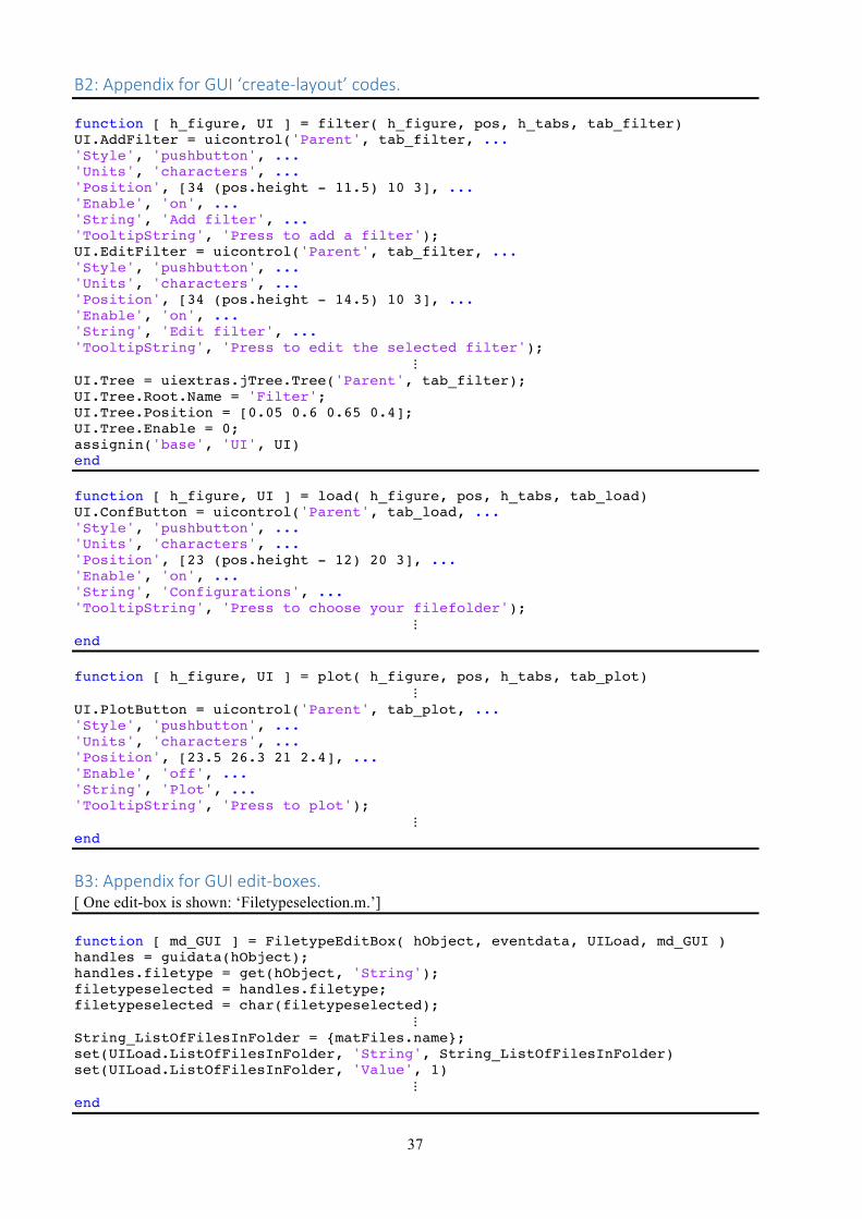
B2:AppendixforGUI‘create-layout’codes. function [ h_figure, UI ] = filter( h_figure, pos, h_tabs, tab_filter) UI.AddFilter = uicontrol('Parent', tab_filter, ... 'Style', 'pushbutton', ... 'Units', 'characters', ... 'Position', [34 (pos.height - 11.5) 10 3], ... 'Enable', 'on', ... 'String', 'Add filter', ... 'TooltipString', 'Press to add a filter'); UI.EditFilter = uicontrol('Parent', tab_filter, ... 'Style', 'pushbutton', ... 'Units', 'characters', ... 'Position', [34 (pos.height - 14.5) 10 3], ... 'Enable', 'on', ... 'String', 'Edit filter', ... 'TooltipString', 'Press to edit the selected filter');

⋮ UI.Tree = uiextras.jTree.Tree('Parent', tab_filter); UI.Tree.Root.Name = 'Filter'; UI.Tree.Position = [0.05 0.6 0.65 0.4]; UI.Tree.Enable = 0; assignin('base', 'UI', UI) end function [ h_figure, UI ] = load( h_figure, pos, h_tabs, tab_load) UI.ConfButton = uicontrol('Parent', tab_load, ... 'Style', 'pushbutton', ... 'Units', 'characters', ... 'Position', [23 (pos.height - 12) 20 3], ... 'Enable', 'on', ... 'String', 'Configurations', ... 'TooltipString', 'Press to choose your filefolder');

⋮ end function [ h_figure, UI ] = plot( h_figure, pos, h_tabs, tab_plot)

⋮ UI.PlotButton = uicontrol('Parent', tab_plot, ... 'Style', 'pushbutton', ... 'Units', 'characters', ... 'Position', [23.5 26.3 21 2.4], ... 'Enable', 'off', ... 'String', 'Plot', ... 'TooltipString', 'Press to plot');

⋮ end

B3:AppendixforGUIedit-boxes.[ One edit-box is shown: ‘Filetypeselection.m.’] function [ md_GUI ] = FiletypeEditBox( hObject, eventdata, UILoad, md_GUI ) handles = guidata(hObject); handles.filetype = get(hObject, 'String'); filetypeselected = handles.filetype; filetypeselected = char(filetypeselected);

⋮ String_ListOfFilesInFolder = {matFiles.name}; set(UILoad.ListOfFilesInFolder, 'String', String_ListOfFilesInFolder) set(UILoad.ListOfFilesInFolder, 'Value', 1)

⋮ end

38

B4:AppendixforGUIbuttons.[ Total of 13 buttons were created, of which parts of ‘Plot.m’ is shown:] function [ ] = Plot(md_GUI) clear d_fn; plot_type_value = md_GUI.plot_type_value; graphtype_X_selected_number = md_GUI.graphtype_X_selected_number; graphtype_X = md_GUI.graphtype_X; experiment_name = md_GUI.selectedloadedfiles; HitsEvents = md_GUI.HitsEvents; experiment_name_01 = char(experiment_name); dimensions = md_GUI.dimension_selected_number; numberofloadedfilesselected = md_GUI.numberofloadedfilesselected; experiment_selected_number = md_GUI.filenumber_selected; selectedloadedfiles = md_GUI.selectedloadedfiles; exp_names = md_GUI.exp_names; p_benjamin_p_d = md_GUI.benjamin_p_d; p_benjamin_p_md = md_GUI.p_benjamin_p_md;

⋮ if plot_type_value == 1 if numberofloadedfilesselected == 1 disp('one exp to plot') exp_name = exp_names{experiment_selected_number}; macro.plot_2(p_benjamin_p_d.(exp_name), p_benjamin_p_md.(exp_name), graphtype_X, experiment_name, dimensions, md_GUI); elseif numberofloadedfilesselected > 1 for l = 1:numberofloadedfilesselected disp('multi exp to plot') exp_name(l) = md_GUI.exp_names(l); end macro.plot_2_n(p_benjamin_p_d, p_benjamin_p_md, exp_name, graphtype_X, experiment_name, dimensions, md_GUI, selectedloadedfiles); end elseif plot_type_value == 2

⋮ end end

B5:AppendixforGUIlist-boxes.[A total of 10 list-box-functions were created, of which parts ‘FilterTreeList.m’ and ‘UI_Tree_selected_node_extract.m’ are shown, of which the latter is a recursive function.] function [ UI, md_GUI ] = FilterTreeList( md_GUI, fileloading ) import uiextras.jTree.* UI.Tree.Enable = 1; if fileloading == 1 filenumber = md_GUI.NumberOfLoadedFiles; filenumber = int2str(filenumber); exp_md = md_GUI.p_benjamin_p_md.(['exp', filenumber]); filename_LoadedFile = char(md_GUI.fileselected(1)); metadata_cond_1 = fieldnames(exp_md.cond); exp_name_in_tree = ['exp', filenumber, '_|_', filename_LoadedFile, '_|_.filter']; elseif fileloading == 2 md_GUI.p_benjamin_p_md.(exp_name) = general.setsubfield(md_GUI.p_benjamin_p_md.(exp_name), base_path, new_ans_1); end Node.Experiment = TreeNode('Name',exp_name_in_tree,'Parent',UI.Tree); [ Node ] = GUI.create_layout.lists.NodeCreator(metadata_cond_1, exp_md, Node)

⋮ end

39

function [ parent, SelectedNode ] = UI_Tree_selected_node_extract( node_depth, parents_nom_str, parent) node_depth = node_depth + 1; node_depth_str = num2str(node_depth); checkingexistanceofUI = evalin('base','exist(''UI'')'); if checkingexistanceofUI == 1 UI = evalin('base','UI'); SelectedNode = UI.Tree.SelectedNodes.Name; parent.(['s', node_depth_str]) = general.getsubfield(UI.Tree.SelectedNodes, parents_nom_str) s_check = strcmp(parent.(['s', node_depth_str]), 'Filter'); if s_check == 0 parents_nom_cut = strsplit(parents_nom_str, '.Name'); parents_nom_str = [char(parents_nom_cut(1)), '.Parent.Name']; [ parent, SelectedNode ] = GUI.create_layout.lists.UI_Tree_selected_node_extract( node_depth, parents_nom_str, parent ) else disp('Depth: ') disp(char(node_depth-1)) end else msgbox('The FilterTreeList is empty.') path = 0; end end

B6:AppendixforGUIpopup-menus.[A total of 10 popup-menu functions were created, of which part of ‘Popup_Hits_or_Events.m’ is shown.] function [md_GUI] = Popup_Hits_or_Events(hObject, eventdata, UILoad, UIPlot, md_GUI) guidata(hObject) disp('Object marked in h or e popup') handles = guidata(hObject); handles.filetype = get(hObject, 'String'); hits_or_events_selected_number = get(hObject, 'Val'); showinformation = 0; if hits_or_events_selected_number == 3 hits_or_events_selected_number = 1; showinformation = 1; end

⋮ if showinformation == 1 information = exps.info; information_comment = information.comment; information_acq_start = information.acquisition_start_str; information_acq_dur = information.acquisition_duration; information_acq_dur = num2str(information_acq_dur); uiwait(msgbox({'File information comment:';information_comment;'Data acquisition start:';information_acq_start;'Data acquisition duration:';information_acq_dur} ,'About !','modal')); hits_or_events_selected_number = 1; set(UIPlot.Popup_Hits_or_Events, 'Value', 1) end hits_or_events_selected = char(hits_or_events_selected); experimenttype = exps.([hits_or_events_selected]); experimenttype_fieldnames = fieldnames(experimenttype); set(UIPlot.Popup_detector_choice, 'Enable', 'on') set(UIPlot.Popup_detector_choice, 'Value', 1)

⋮ md_GUI.experimenttype = experimenttype; end

40

Appendix C: Additional plots. We present, in figure C2, a comparison between the pyridine and the pyridine with water clusters for photon energies above the C-edge (and below the N-edge) has been made, with specific regions highlighted and enhanced.

In figure C1, we notice that the main differences, at which the clusters have higher abundances, are at 14 Da, 16-18 Da, 28 Da, 34-35 Da, (from water groups), 32 Da (O2), 72-74 Da and 78-80 Da whilst the main differences at which the molecules have higher abundances are at 26 Da resp. 49-52 Da. The difference at 73 Da corresponds to a protonated water cluster with n=4 water molecules. It shows that the incident photons are able to ionize the water molecules within the clusters, or, that there is a high abundance of pure water clusters. The only suspicious observations that can be noted in Figure C1 are the peaks of N2, O2, and OH-(H2O)-R with a radical. While N2 and O2 are most likely related to residual gas in the vacuum system, the presence of a radical cannot be explained.

Figure C1: Mass spectra comparison for pure pyridine resp. pyridine in water clusters in the molecular regime. Spectras have been normalized to carbon.