studies in nonlinear dynamics &...

Studies in Nonlinear Dynamics &Econometrics

Volume10, Issue3 2006 Article 7

NONLINEAR ANALYSIS OF ELECTRICITY PRICES

Risk Premia in Electricity Forward Prices

Pavel Diko∗ Steve Lawford†

Valerie Limpens‡

∗Electrabel S.A., [email protected]†Electrabel S.A., [email protected]‡Electrabel S.A., [email protected]

Copyright c©2006 The Berkeley Electronic Press. All rights reserved.

Risk Premia in Electricity Forward Prices∗

Pavel Diko, Steve Lawford, and Valerie Limpens

Abstract

We investigate the presence of significant electricity forward risk premia, using data fromthree major continental European energy markets - German, Dutch and French. We introduce therisk premium in the framework of a standard electricity spot/forward unobserved factor model, andderive the implied forward price behaviour. We then assess the term-structure and time-evolutionof the risk premia for each of the markets.

∗Corresponding author: Pavel Diko. Address: Electrabel, avenue Einstein 2a, 1348 Louvain-la-Neuve, Belgium. Email: [email protected]. Diko, Lawford and Limpens are with theStrategy, Research and Development team, Electrabel SA. We acknowledge support from Electra-bel SA, Jacqueline Boucher and Andre Bihain. All remaining errors are our own. This paper wascompiled using Miktex, and numerical results were obtained using Eviews and Python.

1 Introduction

Early models of electricity market prices that were inspired by the financial literaturegenerally argued that (discounted) forward prices should equal current spot prices. Thisno-arbitrage reasoning was based on a buy-and-hold strategy that works well in typicalfinancial markets yet breaks down in electricity markets due to the non-storable natureof the traded commodity. In a sense, electricity forwards are not strictly speakingderivatives, because their value is not a function of another traded asset. However, theyare basic tradables in the electricity market, and the presence of a properly defined riskpremium in their prices cannot be ruled out.

In this paper, we study the presence of risk premia in three of the most liquid conti-nental European electricity markets: Germany (EEX), France (Powernext: PWN) andthe Netherlands (APX). Our analysis follows and extends the results of recent work byseveral authors. Longstaff and Wang (2004) and Karakatsani and Bunn (2005) bothperform nonparametric analysis of very-short-term forward prices, and spot prices, onthe American PJM, and UK electricity markets, and find evidence of significant risk pre-mia. Villaplana (2003) calibrates a two-factor mean-reverting model with jumps, usinghistorical electricity spot prices on the PJM market and then compares the theoreticalprice of the forward with that quoted on the market, to obtain the risk premium interms of the market price of risk of the underlying risk-factors. The former approachis unable to provide information on the risk premium over longer time horizons, whilethe latter is sensitive to estimation of seasonality patterns in electricity spot price series(robust estimation of seasonality is typically difficult to perform in electricity markets,see e.g. Culot et al. (2006) for discussion).

Our method combines the advantages of the two approaches to provide estimatesof risk premia at various time horizons, while being robust to spot price seasonality.Moreover, we extend the previous work and show an apparent time-evolution of the riskpremia, and a clear reduction in magnitude with progressive maturity of the markets. Wefocus on major European markets - German, French and Dutch - and consider separatelypeak and off-peak prices, as the properties of risk premia have been shown to differempirically for peak and off-peak (see Karakatsani and Bunn (2005)). The theoreticalequilibrium model of Bessembinder and Lemmon (2002) also predicts different behaviourfor peak and off-peak risk premia due to different demand levels in the two periods.The spot price data used in this paper is taken from EEX, PWN and APX, whilethe forward data is taken from Platts, an independent energy market data publishingcompany (further details are given below).

The rest of the paper is organized as follows. In Section 2, we perform a nonpara-metric analysis along the lines of Longstaff and Wang (2004) that shows significant riskpremia in short-term forwards in all three markets. We recast the analysis in a dy-namic trading framework that allows us to demonstrate the time-evolution of the riskpremium. Section 3 introduces a simple forward market model and links the theoreticalnotion of the market price of risk to the results of Section 2. In Sections 4 and 5, wemotivate the use of a three-factor forward market model for real market prices, showthat our main empirical results confirm significant risk premia in forward prices, andoffer a visualization of the risk premium term-structure. Section 6 concludes.

1Diko et al.: Risk Premia in Electricity Forward Prices

Published by The Berkeley Electronic Press, 2007

2 Empirical Motivation

To illustrate, we examine the performance of a hypothetical sliding MWh trading strat-egy (discussed in Hinz et al. (2005)) on each of the markets, for both peakload andoff-peak hours, and consider short-term forwards (namely, day-ahead over-the-counterprices, as published by Platts), and spot prices (exchange average clearing price). Westart with an initial capitalK(0), and repeat the following strategy on each day i ∈ [1, D]:

Buy on Forward On day i, invest all current capital K(i− 1), in order to buy poweron the over-the-counter market (paying the over-the-counter price F (i)).

Sell on Spot Also on day i, resell the power on the spot exchange (receiving the ex-change clearing price S(i)), ending with a new amount of capital K(i).

For instance, if K(0) = 10e, and spot and forward prices are S(1) = 5e/MWhand F (1) = 4e/MWh respectively, then we will buy ρ := K(0)/F (1) = 2.5MWh onthe forward market, and receive ρS(1) = 12.5e from sale on the spot market. Theaccumulated capital at the end of day d ≤ D from pursuing this strategy, assuming nowthat K(0) = 1, is given by K(d) = Πd

i=1S(i)/F (i), so that lnK(d) =∑di=1lnS(i) −

lnF (i). A positive (negative) average risk premium over [1, d] corresponds to lnK(d)greater (less) than zero, i.e. spot price greater (less) than forward price, on average.The accumulated log capital lnK(d) over time, using actual market data, is plotted inFigures 1–6, for EEX, APX and PWN peakload and off-peak hours.

The spot price S(i) is the mean (conditional on peak or off-peak hour) exchangeclearing price for physical delivery of power on day i. Spot prices and volumes oneach of the markets are determined in advance by a two-sided blind auction, organizedby the individual exchanges. Until the morning of the day prior to delivery, marketparticipants may continuously propose price/quantity bid/sell combinations using anelectronic system, for each hour of the delivery day. The bids are entered into a sealedorder book, and upon closure of the bidding phase, are aggregated to give market demandand supply curves for the following day. The intersection of each of these curves givesthe market clearing price and volume by hour. Peak hours are market-specific, and aregiven as: [0700-2300) on APX, [0800-2000) on EEX and [0800-2000) on PWN. For furtherdetails, see the exchange websites www.apx.nl, www.eex.de and www.powernext.fr.

The forward price F (i) is determined on an over-the-counter (bilateral) market, onday i− 1, also for delivery on day i. The sample periods are from 01/2001 to 08/2005,noting that there are no forward quotations on weekends. Returns are calculated relativeto the next trading day. While exchanges give 24 hourly spot prices, set on day i − 1for delivery on i, Platts (see www.platts.com for details) gives base, peak and off-peakflat delivery forward prices, where peak/off-peak hours are the same on the exchangesand the over-the-counter market. The Platts prices are a volume-weighted mean of allover-the-counter deals for delivery on day i executed during day i − 1. There are nogeographical mismatches between the exchange and over-the-counter markets (as mayarise on American markets), nor are there any timing mismatches (since virtually allover-the-counter deals are executed before the spot exchange closes on day i− 1).

Summary descriptive statistics for R(i) := lnS(i) − lnF (i) are given in Table 1,where D is the number of observations (not necessarily consecutive days), E[R] and

2 Studies in Nonlinear Dynamics & Econometrics Vol. 10 [2006], No. 3, Article 7

http://www.bepress.com/snde/vol10/iss3/art7

s.d.[R] are the estimated mean and standard deviation, and τ is the t−statistic thatE[R]= 0. Clearly, there is a very significant negative average short-term risk premiumfor all markets, during peakload hours, over the sample period. We observe a positiveaverage short-term risk premium on EEX off-peak hours, that is significant at the 5%level. There is no significant average risk premium during either APX or PWN off-peakhours.

EEX APX PWNpeak off-peak peak off-peak peak off-peak

D 721 846 698 833 717 842E[R] −0.04211 0.01325 −0.04656 0.00732 −0.02232 0.00545

s.d.[R] 0.19849 0.16361 0.21905 0.24384 0.14428 0.12141τ −5.70 2.36 −5.62 0.87 −4.14 1.30

Table 1: Summary descriptive statistics for R(i) := lnS(i) − lnF (i), i ∈ [1, D], whereR(·) is the one-day risk premium, S(·) and F (·) the spot and forward prices respectively,i the day (observation number), and D the total number of observations in the sample.The sample mean (and corresponding t-statistic, τ) and sample standard deviation, arereported for peak and off-peak hours, on the EEX, APX and PWN power markets.

Note that the slope of lnK(d) represents the instantaneous short-term (one-day)risk premium, which can be approximated on day d by ∆ lnK(d)/∆d, which equalslnK(d) − lnK(d − 1) = lnS(d) − lnF (d) = R(d), given ∆k := 1 − Lk, with L the lagoperator, and k = 1. Further, (1/2)[lnK(d)− lnK(d− 2)] = (1/2)[R(d) + R(d− 1)], ifk = 2, and an m−step backwards moving average of R(d) when k = m. A more accurateapproximation, which is convenient from a graphical viewpoint, is given by constructinga univariate Nadaraya-Watson kernel regression estimator of R(i) on i (days). Thekernel estimator of R(x) at every point x is given by

R(x) = arg minψ

D∑i=1

(R(i)− ψ)2K((x− i)/h),

where D is the number of observations in the sample, and ψ is a locally-fit constant.The bandwidth h controls the degree of smoothing. It is fixed across the sample,and is selected by the “rule-of-thumb” h = 0.15(maxi − mini) = 0.15(D − 1).The kernel weighting function K(u) is chosen to be the Gaussian density function(2π)−1/2 exp(−u2/2). For an introduction to kernel techniques, see Abadir and Law-ford (2004) and references therein. The results are plotted in Figures 7–12, and give aclear indication of time-varying trends in the instantaneous short-term risk premia.

3 Single-Factor Market Model

Here, we introduce the concept of the risk premium in a standard theoretical model of thespot and forward electricity market, that has been analyzed by, inter alia, Clewlow andStrickland (1999). Define a filtered probability space (Ω, F, Ft, P ), where Ft is a (null-set augmented) filtration generated by a one-dimensional Wiener process Wt, and P the



physical measure. We denote by St = exp(Xt) the spot price of electricity for delivery attime t. The time evolution of the log-spot price follows an Ornstein-Uhlenbeck processwith constant speed of reversion α, instantaneous volatility σ and time-varying meanlevel βt, satisfying the stochastic differential equation (SDE)

dXt = α(βt −Xt) + σdWt, α, σ > 0.

The price of a forward contract at time t for delivery at time T ≥ t will be denotedF (t, T ). We assume that at each time t, a forward contract with every maturity T ≥ tcan be traded. As shown by Clewlow and Strickland (1999), in the absence of arbitragethe dynamics of the forward price F (t, T ) under the (unique) risk-neutral measure Qequivalent to P , satisfy the SDE

dF (t, T )F (t, T )

= σe−α(T−t)dWt, (3.1)

where Wt denotes a Wiener process under Q. The risk-neutral dynamics of the wealthKt generated by the continuous time equivalent of the sliding MWh strategy in thismodel are shown in the Appendix to follow

dKt

Kt= σdWt.

As expected, the wealth process of this trading strategy is a Q-martingale. However, ourpreliminary empirical observations show that under the historical probability measureP , the wealth process Kt has a (negative) drift. So, under P we observe that

dKt

Kt= νdt+ σdWt.

From the Cameron-Martin-Girsanov theorem, we have that dWt = dWt + (ν/σ)dt,and by substituting into (3.1) we obtain the implied forward dynamics under the physicalmeasure:

dF (t, T )F (t, T )

= νe−α(T−t)dt+ σe−α(T−t)dWt.

We conclude that in the simple one-factor mean-reverting market model the empiri-cally observed drift in the sliding MWh trading strategy should imply a drift (decreasingwith time to maturity) in the forward contracts. In Section 5, we directly extend theabove argument to a more realistic market model.

3.1 Estimation

In practice, electricity markets quote forwards for delivery over a period of time (forinstance, a week, month, quarter, or year). Let F (t, T1, T2) be the price of a forwardcontract quoted at time t for delivery over the period [T1, T2]. To exclude arbitrage wemust have



F (t, T1, T2) =1

T2 − T1

∫ T2

T1

F (t, s)ds.

For the sake of computationally tractable estimation, we approximate the forwardprice F (t, T1, T2) by assuming that the prices of the forward contracts for a single timedelivery within the period [T1, T2] are approximately equal, i.e. for s, u ∈ [T1, T2] :F (t, s) ≈ F (t, u). Application of Ito’s lemma and rearranging then gives

dF (t, T1, T2)F (t, T1, T2)

= c(t, T1, T2, α)(νdt+ σdWt),

c(t, T1, T2, α) =e−α(T2−t)(1− e(T2−T1+1)α)

(T2 − T1)(1− eα),

where c(·) is derived by infinite series expansions of (T2 − T1)−1∑T2T=T1

exp(−α(T − t)),that arises in (dF (t, T1, T2)/F (t, T1, T2))/(dKt/Kt). Directly, we obtain the followingsystem:

dKt

Kt= νdt+ σdWt, (3.2)

dF (t, T1, T2)/F (t, T1, T2)dKt/Kt

= c(t, T1, T2, α). (3.3)

The parameters ν and σ are estimated by least squares on (3.2), and α is esti-mated by minimizing the mean squared error of the difference between the left andright hand sides of (3.3). Note that (3.2) may be written, after use of Ito’s lemma, asd lnKt = (ν − σ2/2)dt+ σdWt. Discretizing (with one unit of time between consecutiveobservations) gives ∆ lnKt = (ν − σ2/2) + σεt, where εt is N(0,1). Estimation of ν andσ follows by maximum likelihood (least squares). The estimation results obtained forthe German, French and Dutch markets are in Table 2. They are very similar to theinitial nonparametric analysis in Section 2 (indeed, compare Tables 1 and 2), which isunsurprising since a one-factor model only gives enough flexibility to model the strongshort-term risk premium.

The numerical estimation of α in c(t, T1, T2, α) is constrained such that α ∈ [0, 2],due to a flat likelihood surface for α > 2. For the EEX and APX peak products, α = 2,with corresponding half-life 0.35 days. The one-factor model illustrates the focus on theshort-term risk premium, and the main insight is that the half-lives on EEX, APX andPWN peak products are all less than half a day. This analysis is extended through thethree-factor model below, where we did not face the same numerical problems, and theestimation is unconstrained.

4 Principal Components Analysis

Following Clewlow and Strickland (2000), we perform a principal components analysison the empirical (symmetric) covariance matrix Σ of d lnF/F for each market, and for



EEX APX PWNpeak off-peak peak off-peak peak off-peak

ν −0.04211 0.01325 −0.04656 0.00732 −0.02232 0.00545(p-value) 1.22× 10−8 0.01851 1.96× 10−8 0.38620 3.43× 10−5 0.19290

σ 0.19849 0.16361 0.21905 0.24384 0.14428 0.12141α 2 0.202 2 0.278 1.59 0.164

half-life 0.35 3.43 0.35 2.49 0.44 4.23

Table 2: Estimated parameters of the one-factor model. See Section 3.1 and equations(3.2) and (3.3) for further details. The parameters ν and σ are estimated by least squares(the p-value follows directly), and α by nonlinear least squares. The continuous-timehalf-life is calculated as (ln 2)/α, and is reported in days. Results are reported for peakand off-peak hours, on the EEX, APX and PWN power markets.

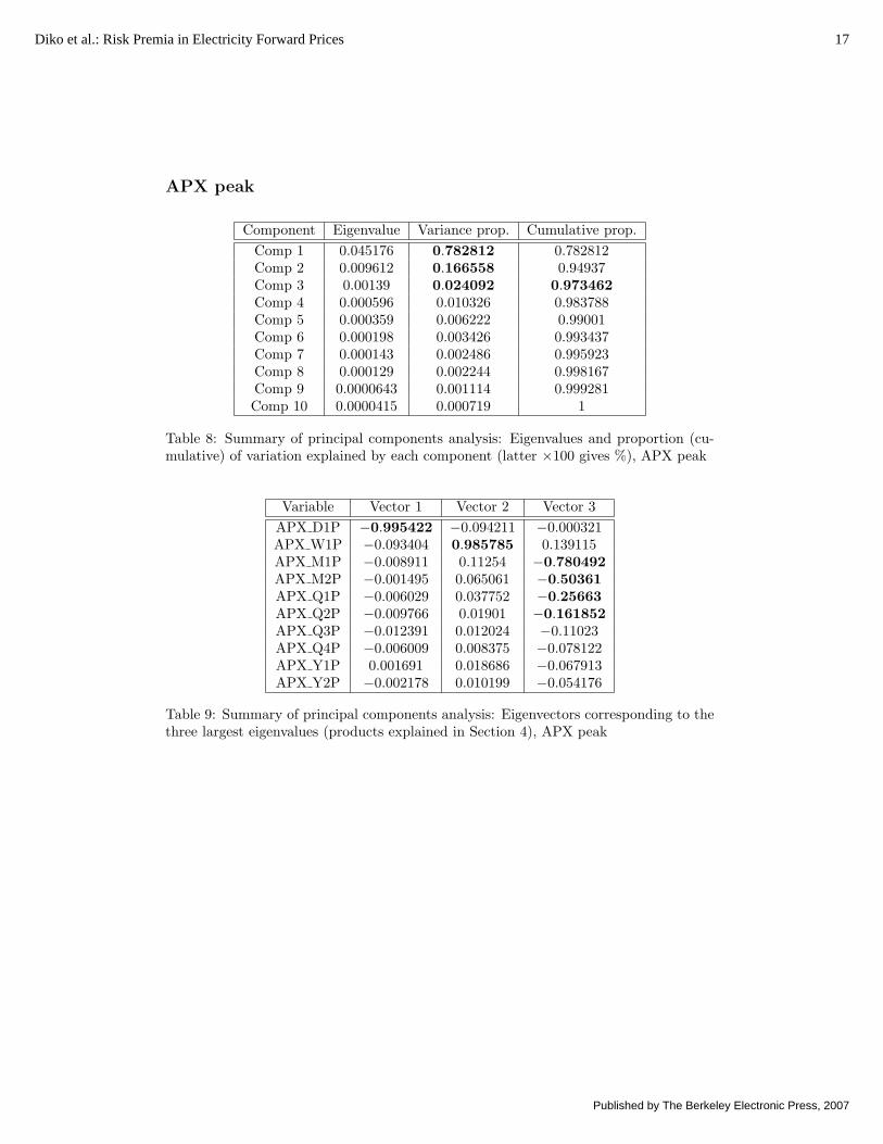
peak and off-peak hours. Since the eigenvectors associated with distinct eigenvalues ofa normal square matrix (ΣΣ′ = Σ′Σ) are orthogonal, we may reduce the dimensionof (d lnF/F ) by sorting eigenvalues in decreasing order of magnitude, and then select-ing only those eigenvectors which contribute “substantially” to explaining the observedvariation in d lnF/F . This gives a guide to determining the appropriate number ofrisk-factors that are needed. Results on eigenvalues and eigenvectors are given in Tables4–15, where elements of eigenvectors that exceed 0.15 in absolute value are highlighted.Notationally, we refer to forward products as (e.g.) EEX D1P, i.e. the day-ahead EEXpeak forward. Other products are W# (week), M# (month), Q# (quarter) and Y#(year), where # denotes a period relative to today, e.g. W1 (forward covering nextweek), and Q2 (forward covering quarter after next). Peak and off-peak products aredenoted by P and OP. For EEX, APX and PWN peak hours, we see that three largestprincipal components explain 95.9%, 97.3% and 96.3% of the variation respectively. ForEEX, APX and PWN off-peak hours, the values are reduced to 89.2%, 91.6%, and 87.5%.

The eigenvectors associated with the three largest principal components have a usefulinterpretation. For instance, on EEX peak hours (Table 5), we see that the first principalcomponent corresponds to short-term effects, through the day-ahead forward. The sec-ond and third principal components correspond to medium-term effects (week-ahead andone-month-ahead and two-month-ahead forwards) and longer-term effects (week-aheadup to three-year-ahead forwards), respectively. Similar results are seen for both APXand PWN peak hours, and for off-peak hours, although the impact of the second andthird principal components at longer time horizons is then reduced. We conclude that athree-factor model is a sensible improvement over the simple one-factor model outlinedabove (at least when considering risk premia), where the three factors correspond toshort-term, medium-term, and longer-term driving forces. We develop this below.

5 Multi-Factor Market Model

We extend the simple market model of Section 3 by introducing three risk-factorsthat drive the electricity spot price. Again, we start with a filtered probability space(Ω, F, Ft, P ) but now the filtration Ft is generated by 3-dimensional Wiener process



Wt = (W 1t ,W

2t ,W

3t ). Multi-factor models have been proposed by several authors as an

appropriate set-up for energy commodities (see e.g. Culot et al. (2006), Koekebakkerand Ollmar (2005) and Schwartz and Smith (2000) for discussion). In this framework,the spot price St = exp(βt + X1

t + X2t + X3

t ), and under the physical measure P thethree risk factors satisfy

dXit = −αiXi

tdt+ σidWit , i = 1, 2, 3.

The forward contracts under the risk-neutral measure follow

dF (t, T )F (t, T )

= σ1e−α1(T−t)dW 1

t + σ2e−α2(T−t)dW 2


t ,

and by the same reasoning as above, the risk-neutral sliding MWh strategy wealth pro-cess satisfies

dKt

Kt= σ1dW

1t + σ2dW

2t + σ3dW

3t ,

and under the physical measure:

dKt

Kt= (ν1 + ν2 + ν3)dt+ σ1dW

1t + σ2dW

2t + σ3dW

3t .

The implied historical forward dynamics are then

dF (t, T )F (t, T )

= (ν1e−α1(T−t) + ν2e−α2(T−t) + ν3e

−α3(T−t))dt

+ σ1e−α1(T−t)dW 1



t .

This formula effectively allows us to use all of the historical forward prices to estimatethe potential risk premium in the forward market at various time horizons. It is alsonoteworthy that the formula does not involve the function βt appearing in the spot priceevolution equation. Hence, our estimation is robust with respect to the seasonality ofpower prices, which can be rather complex and difficult to model.

5.1 Estimation

As for the simple one-factor model above, we approximate the market quoted forwardprices F (t, T1, T2) to facilitate estimation. By direct application of Ito’s lemma, weobtain

dF (t, T1, T2)F (t, T1, T2)

=3∑i=1

c(t, T1, T2, αi)(νidt+ σidWit ).

The stochastic processes Y 1t , Y

2t , Y

3t follow the SDE’s dY it = νidt + σidW

it , i = 1, 2, 3,

and we can rewrite the system to be estimated as:



dY it = νidt+ σidWit , i = 1, 2, 3, (5.1)

dKt

Kt=

3∑i=1

dY it , (5.2)

dF (t, T1, T2)F (t, T1, T2)

=3∑i=1

c(t, T1, T2, αi)dY it . (5.3)

After discretization, the system (5.1)–(5.3) can be viewed as a state-space model withstate and observation vectors (∆Y 1

t ,∆Y2t ,∆Y

3t ), (∆Kt/Kt,∆F (t, T1, T2)/F (t, T1, T2)).

In principle, this can be estimated using the Kalman filter, modified to account for miss-ing data (since we do not observe all the forward prices on all quotation days), and cou-pled with a parameter space search algorithm as in Cortazar et al. (2003) . Kalman filterestimation is, however, strongly dependent on the choice of the observation error covari-ance matrix, which in our case has very large dimension and is not easily parameterized.In addition, the parameter space is large (parameters (α1, α2, α3, ν1, ν2, ν3, σ1, σ2, σ3)),and it is no simple matter to find a global optimum. To overcome this problem, we de-sign a two-step least squares estimation procedure in the spirit of the one-factor modelestimation.

Step 1. Find dY it and αi that minimize (where α1 < α2 < α3)

∑t

(dKt

Kt−

3∑i=1

dY it

)2

+∑

[T1,T2]

(dF (t, T1, T2)F (t, T1, T2)

−3∑i=1

c(t, T1, T2, αi)dY it

)2.

Step 2. Given dY it from Step 1, obtain least squares estimates of νi and σi.

Intuitively, the method first finds (α1, α2, α3) and corresponding (∆Y 1t ,∆Y

2t ,∆Y

3t )

to minimize the model pricing error, and then estimates (ν1, ν2, ν3, σ1, σ2, σ3) as themean and standard deviation of (∆Y 1

t ,∆Y2t ,∆Y

3t ). In the Appendix, we demonstrate

that this estimator is in fact equivalent to the Kalman filter. Parameter estimates foreach of the markets are listed in Table 3.

Of particular note, we see that the half-lives associated with the short-term factor(peak products) are all roughly half a day (and α < 2), and so the one-factor modeloverstates the short-term rate of reversion (see the discussion in Section 3.1).

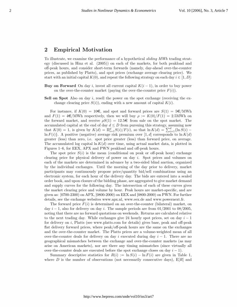
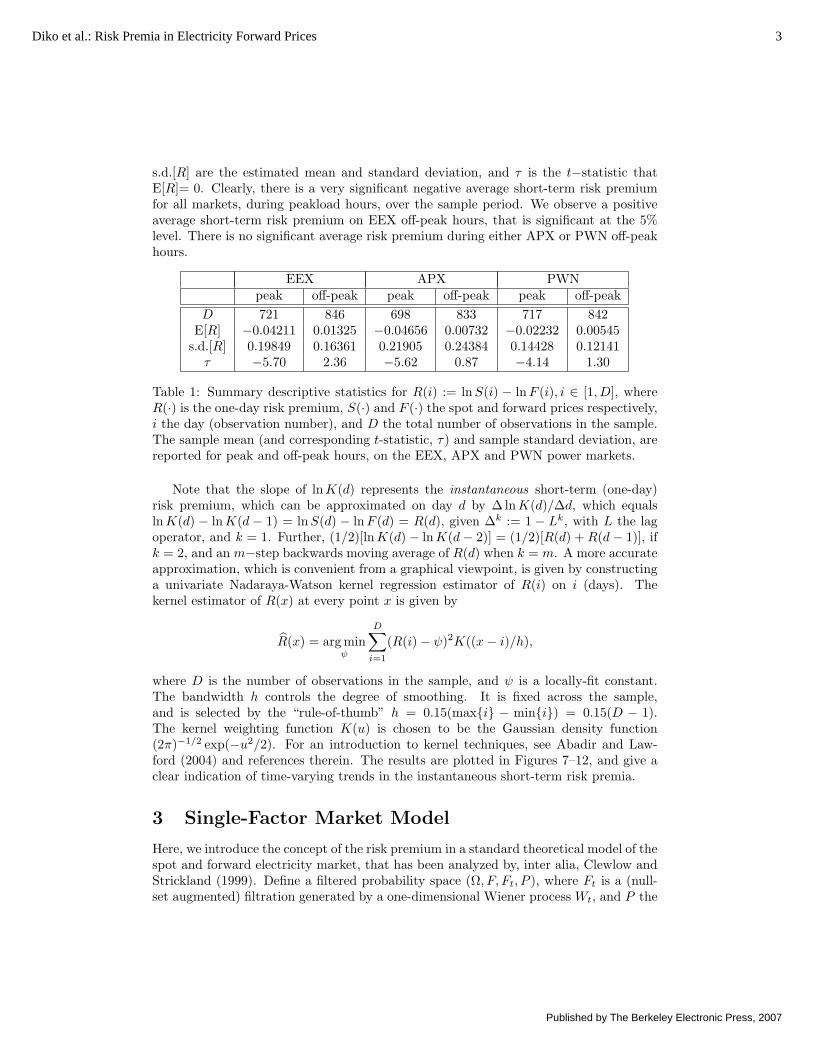
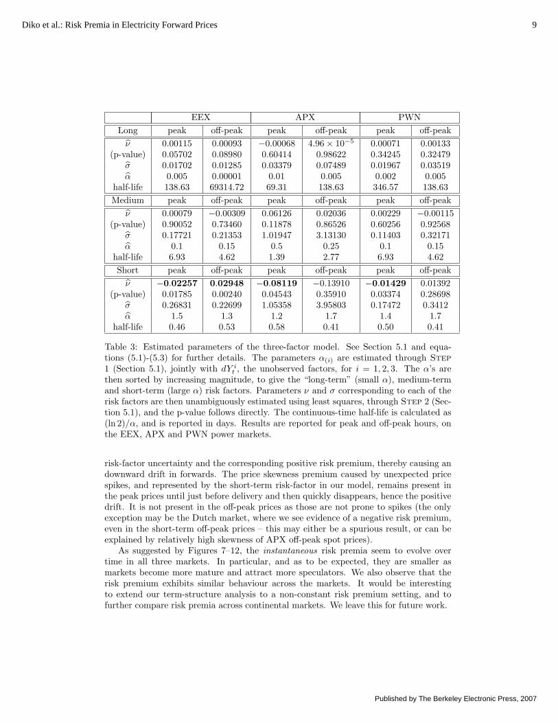
5.2 Term-structure and temporal dynamics of risk premia

Using the estimation results from Table 3, we can visualize the term-structure of the riskpremia; that is, the dependence of the instantaneous drift in the forward prices on thetime to maturity. Figures 13–18 plot these for the three markets under study. The resultsobtained are in very good agreement with the theoretical model of Bessembinder andLemmon (2002), who predict negative risk premia caused by the presence of skewness inthe spot price distribution, and positive risk premia due to the level of volatility in thespot price. As the time to maturity decreases, so does the long-term and medium-term



EEX APX PWNLong peak off-peak peak off-peak peak off-peakν 0.00115 0.00093 −0.00068 4.96× 10−5 0.00071 0.00133

(p-value) 0.05702 0.08980 0.60414 0.98622 0.34245 0.32479σ 0.01702 0.01285 0.03379 0.07489 0.01967 0.03519α 0.005 0.00001 0.01 0.005 0.002 0.005

half-life 138.63 69314.72 69.31 138.63 346.57 138.63Medium peak off-peak peak off-peak peak off-peak

ν 0.00079 −0.00309 0.06126 0.02036 0.00229 −0.00115(p-value) 0.90052 0.73460 0.11878 0.86526 0.60256 0.92568

σ 0.17721 0.21353 1.01947 3.13130 0.11403 0.32171α 0.1 0.15 0.5 0.25 0.1 0.15

half-life 6.93 4.62 1.39 2.77 6.93 4.62Short peak off-peak peak off-peak peak off-peakν −0.02257 0.02948 −0.08119 −0.13910 −0.01429 0.01392

(p-value) 0.01785 0.00240 0.04543 0.35910 0.03374 0.28698σ 0.26831 0.22699 1.05358 3.95803 0.17472 0.3412α 1.5 1.3 1.2 1.7 1.4 1.7

half-life 0.46 0.53 0.58 0.41 0.50 0.41

Table 3: Estimated parameters of the three-factor model. See Section 5.1 and equa-tions (5.1)-(5.3) for further details. The parameters α(i) are estimated through Step1 (Section 5.1), jointly with dY it , the unobserved factors, for i = 1, 2, 3. The α’s arethen sorted by increasing magnitude, to give the “long-term” (small α), medium-termand short-term (large α) risk factors. Parameters ν and σ corresponding to each of therisk factors are then unambiguously estimated using least squares, through Step 2 (Sec-tion 5.1), and the p-value follows directly. The continuous-time half-life is calculated as(ln 2)/α, and is reported in days. Results are reported for peak and off-peak hours, onthe EEX, APX and PWN power markets.

risk-factor uncertainty and the corresponding positive risk premium, thereby causing andownward drift in forwards. The price skewness premium caused by unexpected pricespikes, and represented by the short-term risk-factor in our model, remains present inthe peak prices until just before delivery and then quickly disappears, hence the positivedrift. It is not present in the off-peak prices as those are not prone to spikes (the onlyexception may be the Dutch market, where we see evidence of a negative risk premium,even in the short-term off-peak prices – this may either be a spurious result, or can beexplained by relatively high skewness of APX off-peak spot prices).

As suggested by Figures 7–12, the instantaneous risk premia seem to evolve overtime in all three markets. In particular, and as to be expected, they are smaller asmarkets become more mature and attract more speculators. We also observe that therisk premium exhibits similar behaviour across the markets. It would be interestingto extend our term-structure analysis to a non-constant risk premium setting, and tofurther compare risk premia across continental markets. We leave this for future work.



6 Conclusions

In this paper, we have investigated the presence and structure of risk premia in forwardprices on three major continental European markets – German, French and Dutch.We confirm previous nonparametric results obtained in the literature on the AmericanPJM, and UK markets, and show that the short-term forward prices are not simply theexpectation of the spot prices. We further link the presence of a risk premium with theproperties of the forward price dynamics at all time-horizons, and use it to extend therisk premium analysis beyond the very short-term. Taking into account all the availablehistorical data, we discover the presence of significant risk premia in the long-term aswell as the short-term. We infer the shape of the risk premium term-structure, i.e.the dependence of the risk premium on time to maturity of the forward contract. Wefind that the term-structure is in agreement with the theoretical model of the electricitymarket developed by Bessembinder and Lemmon (2002). It reflects the changing balanceof two forces that determine the risk premium, namely the sensitivity to skewness of thespot price, and the variability of the spot price. As the time to maturity increases, theinfluence of skewness becomes relatively less important compared to the variability, andso the risk premium decreases.



Abadir, K.M., and S. Lawford (2004): “Optimal asymmetric kernels,” Economics Let-ters, 83, 61-68.

Bessembinder, H., and M.L. Lemmon (2002): “Equilibrium pricing and optimal hedgingin electricity forward markets,” Journal of Finance, 57, 1347-1382.

Clewlow, L., and C. Strickland (1999): “Valuing energy options in a one factor modelfitted to forward prices,” Quantitative Finance Research Paper no. 10, University ofTechnology, Sydney.

Clewlow, L., and C. Strickland (2000): Energy Derivatives: Pricing and Risk Man-agement. London: Lacima Publications.

Cortazar, G., Schwartz, E.S., and L. Naranjo (2003): “Term structure estimation inlow-frequency transaction markets: A Kalman filter approach with incomplete panel-data,” Working Paper 6-03, Anderson School of Management, UCLA.

Culot, M., Goffin, V., Lawford, S., de Menten, S., and Y. Smeers (2006): “An affinejump diffusion model for electricity,” mimeo, Electrabel.

Hinz, J., von Grafenstein, L., Verschuere, M., and M. Wilhelm (2005): “Pricing electric-ity risk by interest rate methods,” Quantitative Finance, 5, 49-60.

Karakatsani, N.V., and D.W. Bunn (2005): “Diurnal reversals of electricity forwardpremia,” mimeo, Department of Decision Sciences, London Business School.

Karatzas, I., and S.E. Shreve (1997): Brownian Motion and Stochastic Calculus. Berlin:Springer.

Koekebakker, S., and F. Ollmar (2005): “Forward curve dynamics in the Nordic elec-tricity market,” Managerial Finance, 31, 74-95.

Longstaff, F.A., and A.W. Wang (2004): “Electricity forward prices: A high-frequencyempirical analysis,” Journal of Finance, 59, 1877-1900.

Schwartz, E.S., and J.E. Smith (2000): “Short-term variations and long-term dynamicsin commodity prices,” Management Science, 46, 893-911.

Villaplana, P. (2003): “Pricing power derivatives: A two-factor jump-diffusion ap-proach,” Working Paper 03-18, Department of Industrial Economics, University CarlosIII, Madrid.



Figure 1: Logarithmic wealth process (lnK)against observation number: EEX peak

Figure 2: Logarithmic wealth process (lnK)against observation number: EEX off-peak

Figure 3: Logarithmic wealth process (lnK)against observation number: APX peak

Figure 4: Logarithmic wealth process (lnK)against observation number: APX off-peak

Figure 5: Logarithmic wealth process (lnK)against observation number: PWN peak

Figure 6: Logarithmic wealth process (lnK)against observation number: PWN off-peak



Figure 7: Kernel-fit instantaneous riskpremium R(·) (×100 gives %): EEX peak

Figure 8: Kernel-fit instantaneous riskpremium R(·) (×100 gives %): EEX off-peak

Figure 9: Kernel-fit instantaneous riskpremium R(·) (×100 gives %): APX peak

Figure 10: Kernel-fit instantaneous riskpremium R(·) (×100 gives %): APX off-peak

Figure 11: Kernel-fit instantaneous riskpremium R(·) (×100 gives %): PWN peak

Figure 12: Kernel-fit instantaneous riskpremium R(·) (×100 gives %): PWN off-peak



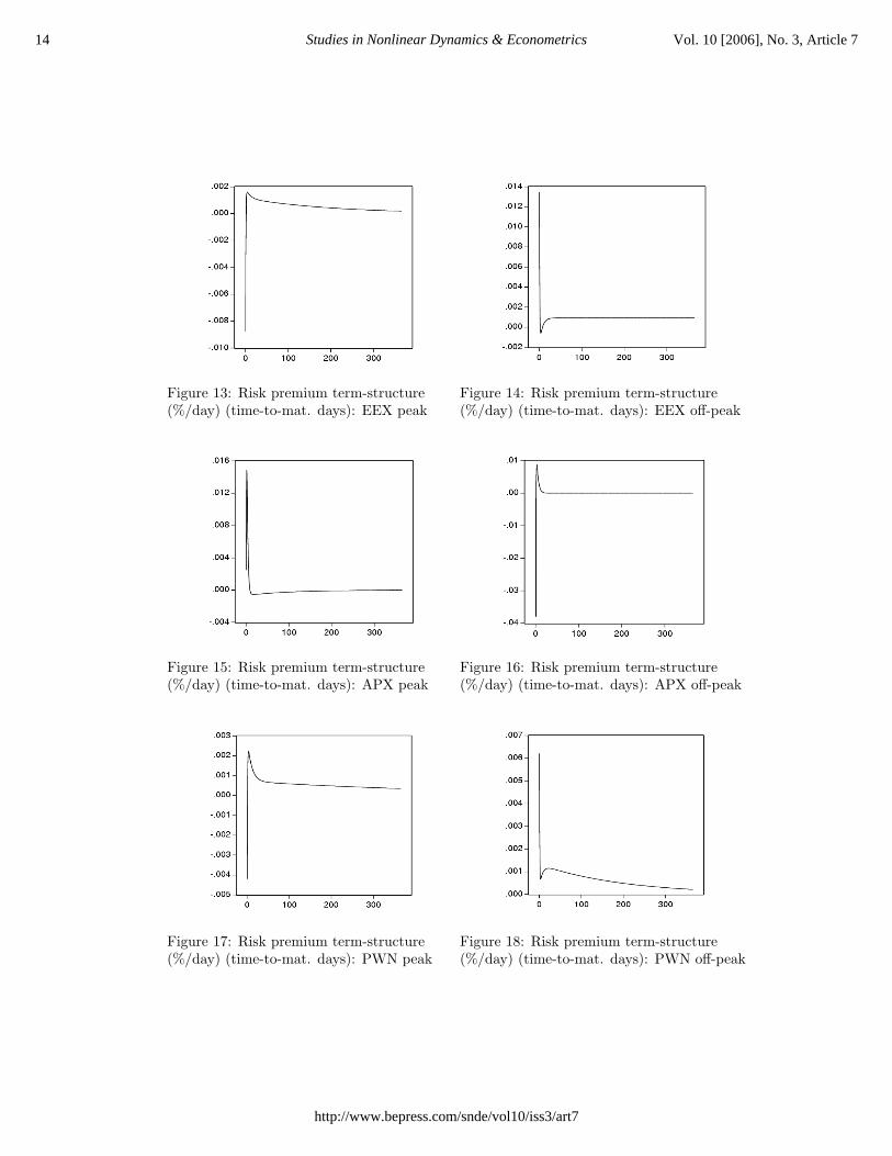
Figure 13: Risk premium term-structure(%/day) (time-to-mat. days): EEX peak

Figure 14: Risk premium term-structure(%/day) (time-to-mat. days): EEX off-peak

Figure 15: Risk premium term-structure(%/day) (time-to-mat. days): APX peak

Figure 16: Risk premium term-structure(%/day) (time-to-mat. days): APX off-peak

Figure 17: Risk premium term-structure(%/day) (time-to-mat. days): PWN peak

Figure 18: Risk premium term-structure(%/day) (time-to-mat. days): PWN off-peak



EEX peak

Component Eigenvalue Variance prop. Cumulative prop.Comp 1 0.028918 0.806624 0.806624Comp 2 0.004474 0.124803 0.931427Comp 3 0.000979 0.02732 0.958747Comp 4 0.000655 0.018279 0.977026Comp 5 0.000244 0.006817 0.983843Comp 6 0.000123 0.00343 0.987273Comp 7 0.0000992 0.002768 0.990041Comp 8 0.0000778 0.002171 0.992213Comp 9 0.0000669 0.001866 0.994079Comp 10 0.0000578 0.001611 0.99569Comp 11 0.0000541 0.001508 0.997198Comp 12 0.0000302 0.000844 0.998042Comp 13 0.0000278 0.000775 0.998817Comp 14 0.0000218 0.000608 0.999425Comp 15 0.0000206 0.000575 1

Table 4: Summary of principal components analysis: Eigenvalues and proportion (cu-mulative) of variation explained by each component (latter ×100 gives %), EEX peak

Variable Vector 1 Vector 2 Vector 3EEX D1P 0.991675 0.126394 −0.014239EEX W1P 0.126809 −0.937227 0.187542EEX M1P 0.020925 −0.25609 −0.368589EEX M2P 0.005448 −0.154066 −0.333433EEX M3P 0.002623 −0.078789 −0.270971EEX M4P 0.000761 −0.006772 −0.287515EEX M5P −0.00296 −0.011587 −0.2266EEX M6P 0.00069 −0.009759 −0.189085EEX Q1P 0.0022 −0.062955 −0.354689EEX Q2P −0.000912 0.00522 −0.239806EEX Q3P −0.000996 −0.045609 −0.091033EEX Q4P −0.001788 −0.036149 −0.105014EEX Y1P 0.000929 0.015394 −0.232396EEX Y2P −0.002161 0.028415 −0.191589EEX Y3P −0.000804 0.037517 −0.425509

Table 5: Summary of principal components analysis: Eigenvectors corresponding to thethree largest eigenvalues (products explained in Section 4), EEX peak



EEX off-peak

Component Eigenvalue Variance prop. Cumulative prop.Comp 1 0.019391 0.687414 0.687414Comp 2 0.003903 0.138377 0.825792Comp 3 0.001868 0.06622 0.892012Comp 4 0.000697 0.024717 0.916728Comp 5 0.000421 0.014909 0.931637Comp 6 0.000386 0.013695 0.945332Comp 7 0.000304 0.010762 0.956094Comp 8 0.000271 0.009612 0.965706Comp 9 0.000237 0.008397 0.974103Comp 10 0.000176 0.006232 0.980335Comp 11 0.000143 0.005058 0.985393Comp 12 0.000121 0.004306 0.989699Comp 13 0.000108 0.003841 0.99354Comp 14 0.000105 0.003724 0.997264Comp 15 0.0000772 0.002736 1

Table 6: Summary of principal components analysis: Eigenvalues and proportion (cu-mulative) of variation explained by each component (latter ×100 gives %), EEX off-peak

Variable Vector 1 Vector 2 Vector 3EEX D1OP 0.995054 −0.089808 −0.03918EEX W1OP 0.094304 0.965934 0.181016EEX M1OP 0.015469 0.06809 0.262071EEX M2OP 0.017821 −0.020692 0.366053EEX M3OP 0.009045 −0.065764 0.316446EEX M4OP 0.004256 −0.103131 0.303805EEX M5OP −0.002925 −0.038423 0.204193EEX M6OP −0.001416 −0.053985 0.168283EEX Q1OP 0.00344 −0.093916 0.417884EEX Q2OP −0.00329 −0.045614 0.238909EEX Q3OP 0.003313 0.016259 0.115969EEX Q4OP 0.011723 −0.007383 0.201498EEX Y1OP 0.003141 −0.110891 0.306071EEX Y2OP 0.002942 −0.074536 0.200298EEX Y3OP 0.010787 −0.073603 0.284638

Table 7: Summary of principal components analysis: Eigenvectors corresponding to thethree largest eigenvalues (products explained in Section 4), EEX off-peak



APX peak

Component Eigenvalue Variance prop. Cumulative prop.Comp 1 0.045176 0.782812 0.782812Comp 2 0.009612 0.166558 0.94937Comp 3 0.00139 0.024092 0.973462Comp 4 0.000596 0.010326 0.983788Comp 5 0.000359 0.006222 0.99001Comp 6 0.000198 0.003426 0.993437Comp 7 0.000143 0.002486 0.995923Comp 8 0.000129 0.002244 0.998167Comp 9 0.0000643 0.001114 0.999281Comp 10 0.0000415 0.000719 1

Table 8: Summary of principal components analysis: Eigenvalues and proportion (cu-mulative) of variation explained by each component (latter ×100 gives %), APX peak

Variable Vector 1 Vector 2 Vector 3APX D1P −0.995422 −0.094211 −0.000321APX W1P −0.093404 0.985785 0.139115APX M1P −0.008911 0.11254 −0.780492APX M2P −0.001495 0.065061 −0.50361APX Q1P −0.006029 0.037752 −0.25663APX Q2P −0.009766 0.01901 −0.161852APX Q3P −0.012391 0.012024 −0.11023APX Q4P −0.006009 0.008375 −0.078122APX Y1P 0.001691 0.018686 −0.067913APX Y2P −0.002178 0.010199 −0.054176

Table 9: Summary of principal components analysis: Eigenvectors corresponding to thethree largest eigenvalues (products explained in Section 4), APX peak



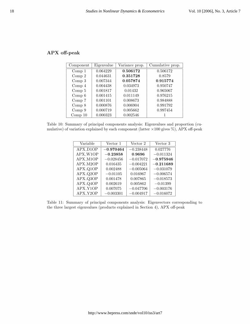
APX off-peak

Component Eigenvalue Variance prop. Cumulative prop.Comp 1 0.064229 0.506172 0.506172Comp 2 0.044631 0.351728 0.8579Comp 3 0.007344 0.057874 0.915774Comp 4 0.004438 0.034973 0.950747Comp 5 0.001817 0.01432 0.965067Comp 6 0.001415 0.011149 0.976215Comp 7 0.001101 0.008673 0.984888Comp 8 0.000876 0.006904 0.991792Comp 9 0.000719 0.005662 0.997454Comp 10 0.000323 0.002546 1

Table 10: Summary of principal components analysis: Eigenvalues and proportion (cu-mulative) of variation explained by each component (latter ×100 gives %), APX off-peak

Variable Vector 1 Vector 2 Vector 3APX D1OP −0.970464 −0.238448 0.027776APX W1OP −0.23858 0.9696 −0.011324APX M1OP −0.028456 −0.017072 −0.975946APX M2OP 0.016435 −0.004221 −0.211689APX Q1OP 0.002488 −0.005064 −0.031079APX Q2OP −0.01105 0.016967 −0.006574APX Q3OP 0.001478 0.007865 −0.018573APX Q4OP 0.002619 0.005862 −0.01399APX Y1OP 0.007075 −0.047706 −0.003176APX Y2OP −0.003301 −0.004917 −0.016072

Table 11: Summary of principal components analysis: Eigenvectors corresponding tothe three largest eigenvalues (products explained in Section 4), APX off-peak



PWN peak

Component Eigenvalue Variance prop. Cumulative prop.Comp 1 0.019741 0.731021 0.731021Comp 2 0.005354 0.198251 0.929272Comp 3 0.00091 0.03371 0.962982Comp 4 0.000404 0.014959 0.977941Comp 5 0.000259 0.009577 0.987518Comp 6 0.000189 0.007007 0.994526Comp 7 0.000148 0.005474 1

Table 12: Summary of principal components analysis: Eigenvalues and proportion (cu-mulative) of variation explained by each component (latter ×100 gives %), PWN peak

Variable Vector 1 Vector 2 Vector 3PWN D1P −0.99371 −0.106958 0.030252PWN W1P −0.091029 0.94107 0.308796PWN M1P −0.054421 0.264436 −0.576325PWN M2P −0.022684 0.142541 −0.505413PWN Q1P −0.023795 0.10449 −0.522919PWN Q2P −0.010231 0.041393 −0.179128PWN Y1P −0.010353 0.008408 −0.102983

Table 13: Summary of principal components analysis: Eigenvectors corresponding tothe three largest eigenvalues (products explained in Section 4), PWN peak



PWN off-peak

Component Eigenvalue Variance prop. Cumulative prop.Comp 1 0.016681 0.556604 0.556604Comp 2 0.007961 0.265644 0.822248Comp 3 0.001567 0.052291 0.874539Comp 4 0.001323 0.044151 0.91869Comp 5 0.001092 0.036435 0.955126Comp 6 0.000784 0.026149 0.981274Comp 7 0.000561 0.018726 1

Table 14: Summary of principal components analysis: Eigenvalues and proportion (cu-mulative) of variation explained by each component (latter×100 gives %), PWN off-peak

Variable Vector 1 Vector 2 Vector 3PWN D1OP −0.995653 −0.08988 −0.010718PWN W1OP −0.08926 0.993245 −0.008249PWN M1OP −0.007825 0.067204 0.389266PWN M2OP 0.006119 −0.026976 0.716039PWN Q1OP −0.02271 0.00765 0.44968PWN Q2OP −0.009645 −0.002484 0.234895PWN Y1OP −0.000947 −0.008835 0.279623

Table 15: Summary of principal components analysis: Eigenvectors corresponding tothe three largest eigenvalues (products explained in Section 4), PWN off-peak



A Appendix: Technical Derivations

Definition 1. Let K(n, t) be the wealth at time t of a trading strategy in which westart with unit wealth, and for each i = 1, . . . , n, we invest all the wealth at time i−1

n t

to buy the electricity futures contract maturing at time in t, and hold that contract until

maturity. We define Kt (the wealth of the sliding MWh trading strategy) to be

Kt = limn→∞

K(n, t).

Proposition 2. The wealth of the sliding MWh trading strategy in the one-factor marketmodel (see Section 3) satisfies the following SDE:

dKt

Kt= σdWt.

Proof. Let us fix a time t. It is easy to see that

K(n, t)K(n, 0)

=n∏i=1

F ( in t,in t)

F ( i−1n t, in t)

,

and taking logarithms on both sides:

lnK(n, t)− lnK(n, 0) =n∑i=1

[lnF

(i

nt,i

nt

)− lnF

(i− 1n

t,i

nt

)]. (A.1)

By direct application of Ito’s lemma, we obtain

lnF(i

nt,i

nt

)− lnF

(i− 1n

t,i

nt

)= −σ

2

4α

(1− e−2αt/n

)+ σ

∫ in t

i−1n t

e−α(it/n−s)dWs.

Substituting into (A.1) and rearranging gives

lnK(n, t)− lnK(n, 0) = −σ2

4αn(1− e−2αt/n

)+ σ

∫ t

0

h(n, s)dWs, (A.2)

where for s ∈ [ i−1n t, in t], h(n, s) = e−αit/n−s, with i = 1, . . . , n. It is clear that

limn→∞

n(1− e−2αt/n) = 2αt. (A.3)

Since limn→∞∫ t0|h(n, s)−1|ds = 0, we have by elementary properties of the Ito integral

(see for example Karatzas and Shreve (1997)) that

limn→∞

∫ t

0

h(n, s)dWs = Wt. (A.4)

Taking the limit in (A.2), and substituting from (A.3) and (A.4), we get



lnKt − lnK0 = −σ2

2t+ σWt.

Rewriting this in differential form, and further application of Ito’s lemma completes theproof.

Corollary 3. In the three-factor market model, the wealth of the sliding MWh strategysatisfies

dKt

Kt=

3∑i=1

σidWit .

The proof is straightforward, and closely follows that above.

Proposition 4. Given a series of observations Ztrt=1, Zt ∈ Rm and matrices Htrt=1,Ht ∈ Rm×n, denote:

X∗t = argmin

Xt∈Rn

r∑t=1

(Zt −HtXt)2, ξ∗t = Zt −HtX∗t , R∗ = cov(ξ∗t ), Q∗ = cov(X∗

t ).

Now consider a state-space model of the form:

Zt = HtXt + ξt, Xt = d+ εt,

where X, d ∈ Rn, εt ∼ i.i.d.N(0, Q∗), and ξt ∼ i.i.d.N(0, R∗). Further, denote by Xtrt=1

the Kalman filter estimator of the state sequence Xtrt=1 given the observation sequenceZtrt=1. Then,

X∗t = Xt; t = 1, . . . , r.

Proof. The equivalence follows from the following set of equations:

Xt = E[Xt|Z1, . . . , Zt]= E[Xt|Zt]= cov(Xt, Zt)var(Zt)−1Zt

= cov(X∗t , Zt)var(Zt)−1Zt

= cov((H ′tHt)−1H ′

tZt, Zt)var(Zt)−1Zt

= (H ′tHt)−1H ′

tvar(Zt)var(Zt)−1Zt= X∗

t ,

where the second equality follows from the independence structure of the state-spacemodel, the third is a standard result from multivariate regression theory, the fourth isimplied by the choice of matrices Q∗ and R∗, and the fifth and the last by the fact thatX∗t is a least-squares estimator.



studies in nonlinear dynamics &...

Documents