studies in ion source development for application in heavy

Studies in Ion Source Development for

Application in Heavy Ion Fusion

Project Report

Master of Science Nuclear Engineering

University of California, Berkeley

Jonathan G. Kapica

May 2004

J. G. Kapica ii MSNE Project

Contents

1. INTRODUCTION TO PROJECT 1

1.1 Objective and Requirements for HIF 1

1.2 STS 50 and Aluminosilicate Sources 2

1.3 STS 100 and Plasma Sources 4

2. ALUMINO-SILICATE SOURCE DC PULSE EXPERIMENTS 5

2.1 Introduction to Experiment 5

2.2 DC Power Supply Design and Construction 5

2.3 Potassium Alumino-silicate Source 7

2.4 Cesium Alumino-silicate Source 14

2.5 Conclusion from Experiment 16

3. TIME OF FLIGHT MEASUREMENTS OF DC BEAM 17

3.1 Motivation and Basic Principle of Experiment 17

3.2 Experimental Setups 17

3.3 Experimental Results 19

3.4 Development of Model and Comparison to Measured Data 25

3.5 Contaminated Cs Source 29

3.6 Conclusions from Experiment 32

4. ALUMINO-SILICATE SOURCE LIFETIME EXPERIMENTS 33

4.1 Setup and method of measurement 33

4.2 Experimental Results 33

4.3 Conclusions 38

5. PLASMA SOURCE ENERGY ANALYZER EXPERIMENT 39

5.1 Introduction 39

5.2 Principles and Theory 40

5.2.1 Optics of a Thin Lens 40

5.2.2 Energy Analyzer Principles 42

5.2.3 Charge Exchange in the Diode Gap 45

J. G. Kapica iii MSNE Project

5.3 Experiment Setup 48

5.3.1 Source Setup 48

5.3.2 Energy Analyzer Setup 48

5.3.3 High Voltage Pulse 50

5.4 Single Beam Results 51

5.4.1 Adjustments to Instrument 51

5.4.2 Argon Gas Pressure Variations 53

5.4.3 Scanning of Electrode-Voltage 53

5.4.4 Asymmetric Electrode-Voltage Test 55

5.5 Combined Beam Results 55

5.6 Energy Spread Due to Charge Exchange 57

5.7 Conclusions 59

6. REFERENCES AND ACKNOWLEDGMENTS 60

J. G. Kapica Page 1 Chapter 1 MSNE Project

1. Introduction to Project 1.1 Objective and Requirements for HIF

The overall purpose of these experiments is to contribute to the development of ion

injector technology in order to produce a driver for use in a heavy-ion-fusion (HIF)

power generating facility. The overall beam requirements for HIF are quite demanding; a

short list of the constraints is the following:

• Low cost (a large portion of overall cost will come from the beam system) • Bright, low emittance beam • Total beam energy 5MJ • Spot size 3mm (radius) • Pulse Duration 10ns • Current on target 40kA • Repetition Rate 5Hz • Standoff from target 5m • Transverse Temp <1keV

Figure 1.1. Layout of basic linear accelerator used for generating the required beam energy on target for HIF. (Figure taken from UCB Tutorial on Heavy-Ion Fusion).

The reasons for employing ion beams in inertial fusion systems become obvious

when the repetition rate required is considered. While laser drivers are useful in

producing a proof-of-concept, they will be incapable of application in power generation.

Consequently attempts in the U.S. to achieve a power generating system make use of

linear ion accelerators. It is apparent that the accelerator system requires the highest


quality input as obtainable. Therefore injector design is an essential portion of the entire

inertial fusion system.

At Lawrence Berkeley and Lawrence Livermore National Laboratories experiments

are being conducted using two injector formats. For this project I have conducted a series

of studies using both. The next two sections provide a brief description of the sources

used for my experiments.

1.2 STS 50 and Alumino-Silicate Sources

The STS 50 test stand located at LBNL and shown in figure 1.2 consists of a small

vacuum chamber containing a themionic ion gun, diagnostics such as a Faraday cup, slit

scanners, neutral-detector, and a time-of-flight measuring apparatus.

Figure 1.2. STS50 ion source test stand at LBNL.

Vacuum is maintained by combining a roughing pump and turbo pump. Pressure is

monitored with a cold cathode and for most experiments operates in the 1x10-7 T range.

The ion gun holds a ¼ inch diameter tungsten source (coated with alumino-silicate) in a

heat shielded cup containing tungsten heating filaments shown in figure 1.3. Power is


supplied to filaments by an isolation transformer. Figure 1.4 shows a side view of the

assembled gun displaying the extraction gap. The gap distance is adjustable and the

source fits into a Pierce electrode. The Pierce (not seen in picture) provides a shaped

acceleration potential to produce a laminar beam with uniform current density.

Figure 1.3. ¼ inch source used in STS50. Source shown with heating system.

Figure 1.4. Ion gun assembly used in STS 50.

Extraction pulses are generated with two different systems for these experiments.

The initial testing was conducted with a bi-polar ±35kV thyratron-triggered pulse


forming network. For most of the experiments, however, a long duration low voltage,

±2.5kV, supply was used. This supply is discussed further in section 2. Extensive

discussion regarding the development and fabrication of the alumino-silicate source is

contained in the two references Chacon-Glocher, E., 2002, and Baca D., et al. 2003.

Alumino-silicate, surface ionization sources provide reliable and relatively long-life

performance and have been a preferred choice for experimentation due to their simplicity

and low cost.

1.3 STS 100 and Plasma Sources

STS 100 at LLNL is the ion source used for the energy spread experiments. It

operates with an RF driven plasma source. The source is configured with a 26cm inner

diameter cylindrical plasma chamber, multi-cusp permanent magnet confinement, 11

MHz / 20µs RF pulse, through a 2 turn 11cm antenna. Ar gas is fed through a time

controlled puffer valve. The multi-beam array consists of a 61 hole grid in a hexagonal

pattern. The beam forming plate contains 2.2 mm Pierce cones, the extraction plate has

matching 4.0mm holes and the gap between the plates is 1.6cm, capable of holding 80kV.

The pulser is capable of 100kV, 20µs pulses, produced from a spark-gap triggered

system. The primary diagnostic used for this project was an electrostatic energy

analyzer, which is discussed at length in chapter 5.


2. Alumino-Silicate Source DC Pulse Experiments 2.1 Introduction to Experiment

The following series of experiments have been conducted to better understand the

performance of an alumino-silicate source for applications in heavy-ion and magnetic

fusion systems. Of interest is the diffusion of ions from the source and the resulting

current from applying a long DC extraction potential. Additionally, from long extraction

periods, the characteristics of the source over the lifetime can be studied. The

experiments have been performed at LBNL on the STS50 Ion Source Test Stand, using a

¼ diameter (A=0.317cm2) tungsten substrate source.

2.2 DC Power Supply Design and Construction

In order to accomplish this series of long pulse-length experiments a power supply

and switching system was constructed. To achieve the desired extraction pulse the

system was required to provide long pulses up to 24hrs, supply steady pulse with constant

voltage regardless of beam loading, switch on and off easily with signal generator input,

and output + and 2.5kV. The system was built using two high-voltage insulated gate

bipolar transistors (IGBT). A functional schematic of the system is shown in figure 2.1.

The IGBT serves as a switch to apply the power supply output to the respective electrode

on the ion gun. Each IGBT is controlled by a driver that applies the appropriate bias

voltages to turn the device on or off. To isolate high-voltage, the drivers are connected to

the signal generator through analog to optical converters. A sample of the system output

is shown in figure 2.2.


Figure 2.1. DC power supply setup.

Figure 2.2. Oscilloscope image showing three traces: 1 - positive 2.5kV extraction

voltage, 3 - signal generator pulse 5V, 4 - faraday cup signal 19.4mV. All shown on a 100ms/div scale.

The following series of tests was run to verify proper operation of the system. A

sample of results is plotted in figure 2.3. The unusual shape of the decay and the

properties of the steady state value will be investigated in the following and future

experiments.

Signal Generator

Analog to Fiber-optic transmitter

IGBT Driver

Positive Power Supply

+IGBT

Analog to Fiber-optic transmitter

−IGBT Negative Power Supply

IGBT Driver

+Out (Pierce

Electrode)

−Out (Extractor

Plate)


-0.2

0

0.2

0.4

0.6

0.8

1

1.2

1.4

1.6

-1 1 3 5 7 9 11 13 15 17 19 21 23 25Time (sec)

J (m

A/cm

2)

2sec5sec7.14sec10sec20sec25sec

Figure 2.3. Beam current density at various pulse lengths at 5kV temp 1100C.

2.3 Potassium Alumino-Silicate Source

This series of experiments was conducted with a Potassium alumino-silicate source.

Originally the STS50 test stand was equipped with a 50kV short (20µs) duration Marx

pulse system. To gain an understanding of this system and the operating characteristics

of the ion gun at these low extraction voltages, beam current was compared to previous

results. Shown in figure 2.4 is a comparison of the current density from the 5kV DC setup

to previously recorded data on the 50kV setup. The current varies significantly for the

duration of the long pulse. In order to compare DC to fast pulse results, the DC signal is

measured a two points, the initial peak and the steady-state value at the tail. Initially

beam current peaks at a value that is clearly space-charge limited and is shown in the

graph of figure 2.4. As expected, the peak current density scales proportional to V3/2.


0.0001

0.001

0.01

0.1

1000 10000 100000Extraction Voltage (V)

J (A

/cm

3)

HV-AC Pulse

LV-DC Pulse

V 3/2

Figure 2.4. J vs. V curves for high voltage AC pulses (20µs) and peak values from the

low voltage DC pulses (500ms), temperature 1090ûC.

For the following test, the affect of source temperature on the peak and steady state

values of current density is determined using the following setup:

• Chamber pressure 3.4X10-7T for entire experiment • Suppressor voltage -800V • Faraday cup directly connected to scope internal 50Ω load (spark-gap used

for scope protection) no bias voltage applied. • Data taken in order of ascending temperature • Temperatures measured with pyrometer before and after data acquisition

Starting with source temperature at 1050ûC, recorded the FC signal at five voltages 1

to 5kV in 1kV steps using 5ms pulse length. The same set of data was taken at 1105 and

1175ûC and the results, plotted on a log scale in figure 2.5. Once again peak values were

used.

From the graph of figure 2.5 it can be seen that at 1105ûC and 1175ûC current appears

to be space-charge limited, while at 1050ûC it is emission limited.


0.1

1

10

1000 10000Extraction Voltage (v)

Curre

nt D

ensi

ty (m

A/cm

2)

117511051050V 3/2

Figure 2.5. Current density vs. Extraction voltage (1-5kV) at three temperatures(ûC).

After the data for the 1050ûC case in figure 2.5 was obtained, a few long pulses

(10sec) were run and caused an increase in the cup current for the same voltage. To

better understand this difference the current-density vs. voltage data was retaken and is

shown in figure 2.6. The temperature was measured before and after each data run and

was constant within the accuracy of the pyrometer, however this method only measures

the temperature of the source surface. The long pulse apparently causes some type of

conditioning making the source operate closer to the space-charge limit. This effect has

been noted in many other cases and appears to be a characteristic property of the

alumino-silicate sources. I believe current flow from the source produces heat from i2R

losses, and more evenly heats the source internally. Once the source conditions it

continues to operate at the higher current until it is shutdown or depleted.


0.1

1

10

1000 10000Extraction Voltage (v)

Cur

rent

Den

sity

(mA

/cm

2)

Second RunFirst RunV 3/2

Figure 2.6. Density vs. Voltage at same temp after several long pulses.

The following set of figures (2.7 2.9) is shown to display the long pulse time

characteristics of the source and the effects of source temperature. In figure 2.7 the

1050ûC case droops more while 1105ûC and 1175ûC cases hold fairly constant. This

shows a difference in ion diffusion rate from the source as a function of temperature.

Clearly operating the source at higher temperatures maintains a more uniform current

density for the duration of the pulse. When the length of the extraction is pushed out to

20sec the resulting behavior becomes interesting and is shown in figure 2.8. Here the

1050ûC case drops off significantly and displays a double decay rate possibly indicating

two different diffusion rates.

0

0.2

0.4

0.6

0.8

1

1.2

1.4

1.6

-0.1 0 0.1 0.2 0.3 0.4 0.5 0.6 0.7Time (s)

FC C

urre

nt D

ensi

ty (m

A/c

m2)

T-1175

T-1105

T-1050

Figure 2.7. 500ms pulse at 5kV for different source temperatures.


0

0.2

0.4

0.6

0.8

1

1.2

1.4

1.6

-5 0 5 10 15 20 25Time (s)

FC C

urre

nt D

ensi

ty (m

A/c

m2)

T-1175

T-1105

T-1050

Figure 2.8. 20 second pulse at 5kV.

The dramatic change in diffusion rate is clearly seen in figure 2.9 for all temperatures.

All three cases decay to a steady state level. The steady state level appears to be a

function of temperature.

0

0.2

0.4

0.6

0.8

1

1.2

1.4

1.6

-5 5 15 25 35 45Time (s)

FC C

urre

nt D

ensi

ty (m

A/c

m2) T-1175

T-1105

T-1050

Figure 2.9. 50 second pulse at 5kV.

Figure 2.10 shows the behavior of the 1175ûC case past the 50 second point, at which

it slowly tapers off to a value slightly higher than the two lower temperature cases.


0

0.2

0.4

0.6

0.8

1

1.2

1.4

1.6

-10 10 30 50 70 90 110Time (s)

FC C

urre

nt D

ensi

ty (m

A/cm

2)

50sec

100sec

Figure 2.10. 100 and 50 second pulses 1175ûC at 5kV.

In an attempt to explain the decay rate the curves were fitted using the following

equations:

∆−=

τtJJ o exp

=

TQ

o expττ

T is temperature in units of energy and Q is desorption energy of the species. Two

decay rates of figure 2.11 may be result of two ion species. Species one depletes as

function of τ1 and the second species depletes at a rate proportional to τ2. From the

values of these rates it can be seen that τ1 is half τ2. It appears from the above equations

the only variable in τ that changes is Q which is a property of the species.


0.3

0.5

0.7

0.9

1.1

1.3

1.5

0 20 40

Time (s)

FC C

urre

nt D

ensi

ty (m

A/cm

2)

100sec

τ1=35

τ2=70

Figure 2.11. Close-up of figure 2.10 showing decay rates with fitted exponential curves.

After about 50 seconds for this source, beam current appears to decay to a fairly

stable steady-state value. During quick pulses (on the order of µs) with adequate rest

between shots, the source has an opportunity to replenish the ion density in the extraction

gap to a space-charge limit. However, during the DC condition, ions are continuously

cleared from the gap and at this point the emission of ions from the source should be

equal to beam current. The emission limited results shown in figure 2.12 were obtained

by measuring the average beam current of the last 50ms of 50sec long pulses.

0.09

0.21

0.320.40

0.48

0.06

0.140.19

0.23 0.25

0.01

0.1

1

1 10Extraction Voltage (kV)

Cur

rent

Den

sity

(mA

/cm

3)

v 3/2

1015F

935F

Figure 2.12. J vs. Voltage during the steady state value of the last 50ms of a 50sec pulse.


2.4 Cesium Alumino-Silicate Source

The following results were obtained using a ¼ Cesium Alumino-silicate source.

Figure 2.13 shows the operating regions of 500ms pulses at varied temperatures. For the

1 to 5kV results, the peak values were seen during the first 4ms of the pulse, and the tail

values are taken from an average of the last 100ms of the pulse. The 20 to 50kV values

were obtained from 20µs pulses generated using the STS50 high-voltage Marx PS. The

peak DC values and the AC results follow the space-charge limit, while the steady-state

values are clearly emission limited.

0.01

0.1

1

10

100

1 10 100

Extraction Voltage (kV)

J (m

A/cm

2)

1110 Peak

1050 Peak

1110 Tail

1050 Tail

V 3/2

Figure 2.13. J vs V for Cesium source

The results for three temperatures are shown in figure 2.14. Overall the temperature

required for peak current density from the Cs source is lower than that required for K,

which is expected due to the lower work function of Cs. Cs behaves in a manner much

easier to predict. These results show no sign of the double decay rate seen in the K

source.


0

0.2

0.4

0.6

0.8

-0.1 0.1 0.2 0.3 0.4 0.5 0.6Time (s)

FC C

urre

nt D

ensit

y (mA

/cm2) T-1175

T-1110

T-1050

Figure 2.14. 500ms Pulse at 5kV for 3 temperatures.

For comparison figure 2.15 shows the difference between the K and Cs sources. As

expected the current for Cs is much lower than K, which can easily be explained due to

the equal kinetic energy but different ion mass. Each beam is given kinetic energy of:

kVmvKE 521 2 ==

However, given the different mass the velocity of each is different:

84.1==K

Cs

Cs

K

mm

vv

Because current is charge per time, the velocity ratio is directly proportional to the

magnitude of current. By comparing the initial peak values of the signals shown in figure

2.15, this appears to hold roughly true.

87.175.04.1 ==

Cs

K

II


0

0.2

0.4

0.6

0.8

1

1.2

1.4

-0.1 0.1 0.2 0.3 0.4 0.5 0.6Time (s)

FC C

urre

nt D

ensi

ty (m

A/c

m2)

K-1175

K-1105

K-1050

Cs-1175

Cs-1110

Cs-1050

Figure 2.15. K compared to Cs

2.5 Conclusion from Experiment

The K alumino-silicate source is capable of long duration pulses with fairly constant

high current when operated in the 0.5 sec range. At longer pulse lengths the beam

undergoes a rapid decay to a semi-steady-state condition at a current roughly 75% lower

than initial value. While this is interesting for lifetime determination, it seems too low to

be of any practical value. If the half second pulse is used repetitively, an important

determination would be the duty cycle. At this time that study has not been conducted.

A verifiable explanation for the double decay rate of the K source has not yet been

developed. The suspicion of contamination of the source coating can not be ruled out; in

fact the result is not always repeatable with all K sources. Included in this report is a

time-of-flight experiment used to test for such contamination. The K sources used for

those tests displayed no signs of contaminates, however they also did not display the

double decay rate.


3. Time of Flight Measurements of DC Beam 3.1 Motivation and Basic Principle of Experiment

The following TOF experiments were conducted with two different setups, one with a

Faraday cup, and the other with a flat plate collector. Four different alumino-silicate

sources (3 Cs, and 1 K) were used. The goal of these experiments was to determine

the makeup of the beam, to insure no impurities were being emitted along with the

chosen ion (K or Cs). From previous experiments with a K source it was thought that

perhaps impurities were causing the unusual DC beam results. During these TOF

experiments, however, it became necessary to make several iterations to the setup to

properly understand the results. The outcome is a better understanding of beam physics

during a TOF test, and a useable design for testing the purity of an ion beam.

As a DC beam passes through a ring, a quick (100ns) pulse is applied; the time it

takes for the perturbation of the beam to appear in the collector is measured. With the

time, distance and ion mass data, calculations can be performed to determine the makeup

of the beam.

With this understanding of the setup and results, more accurate beam energy

measurements can be made by reversing the calculation and assuming the mass of the

ion.

3.2 Experimental Setups

Each setup is shown below with brief explanations. The initial setup consisted of a

timing ring and a Faraday cup with the layout shown in figure 3.1. With this setup it was

very difficult to decipher the data because it was obtained with the scope in the 100%

band width mode, and the capacitive noise from the ring made the signal nearly useless.


To clean up the signal the cup opening was covered with a screen, all cables inside the

vacuum chamber were heavily shielded, and the scope was switched to 20% band width.

The resulting signal was significantly improved and is shown in the following results

section.

Figure 3.1. Initial TOF experimental setup with Faraday cup.

After observing results from the faraday cup setup, it was determined that a more

definitive impact position was needed to obtain useful results. To resolve ambiguity, a

simple flat plate was installed in place of the faraday cup as shown in figure 3.2. The

plate was hooked into the scope with a 50Ω resistance.

Figure 3.2. TOF experimental setup with flat plate collector.

During the development of the model shown in section 3.4, the effect of the field after

the ring presented some confusion. To obtain better defined electric fields, a ground plate

9.5 1

Collector Plate

Source TOF Ring

ExtractorPlate

5.5 1

Faraday Cup

Source

TOF Ring

Extractor Plate

11


was installed after the ring (figure 3.3). Now the field after the ring is terminated in a

clear plane.

Figure 3.3. TOF setup with GND plate installed.

3.3 Experimental Results

With the screen installed over opening to FC the signal strength was lower but the

output was cleaned up enough to see the desired timing signal. Figure 3.4 shows a

composite of data taken for four different extraction voltages. The timing signal

elongated and moved later in time as expected with the lower beam energies.

-0.5

0

0.5

1

1.5

2

0.0 1.0 2.0 3.0 4.0 5.0 6.0 7.0 8.0Time (µs)

FC S

igna

l (m

V)

2.5 kV

2 kV

1.5 kV1 kV

Figure 3.4. Faraday cup signals for varied extraction voltages using Cs source and

+800V, 200ns pulse on the timing ring.

8 1

Collector Plate

Source

TOF Ring

Extractor Plate

1.5

GND Plate


To further validate the output, the polarity of the ring voltage was reversed and as

expected, the signal inverted (figure 3.5). More noticeable in this set of graphs is the

second pulse further in time. This is believed to be caused by the FC geometry.

0

0.5

1

1.5

2

2.5

0.0 1.0 2.0 3.0 4.0 5.0 6.0 7.0 8.0Time (µs)

FC S

igna

l (m

V)2.5 kV

2 kV

1.5 kV1 kV

Figure 3.5. Faraday cup signals for varied extraction voltages using Cs source and -

800V, 200ns pulse on the timing ring.

To illustrate this more clearly, shown in figure 3.6, are the calculated times to front

edge (5.5) and the back (11) of the cup. Apparently the beam spread is significant

enough at 6.5 from the extraction plate to scrape the front edge of the cup and cause the

first timing pulse. Then subsequently the remainder of the beam impacts the back of the

cup causing the later pulse.

0

0.5

1

1.5

2

2.5

3

0.0 1.0 2.0 3.0 4.0 5.0 6.0 7.0 8.0Time (µs)

FC S

ignal

(mV)

2.5kV (+800)

2.5kV (-800)

5.5"

11"

Figure 3.6. TOF pulses for Cs. Positions for 5.5 and 11 were calculated and labeled

to show correlation with timing signals.

For the calculations the following simple energy equation and mass data was used:


2

2mvqE = ; tdv =

Ion Atomic mass mass kg

Cesium Cs 132.90545 2.207 x 10-25 kg Potassium K 39.0983 6.493 x 10-26 kg

As can be seen from figure 3.6, the measurement point is at the beginning of the

perturbation. This point of the signal is used for all subsequent measurements. By

conducting this measurement for all beam energies and plotting versus calculations,

figure 3.7 shows the close correlation between the two. Error for these measurements is

all below 3%

3.68

3.05

2.62

2.39

3.67

3.00

2.32

2.59

2

2.5

3

3.5

4

1 1.5 2 2.5Extraction Voltage (kV)

TOF

(µs)

Measured (+800V)

Calculated

Figure 3.7. Cs source - Comparison of pulse timing to calculation for the front of FC

(5.5 inches).

The following figures (3.8 3.10) show the results from a K source using the Faraday

cup. These differ, as expected, from the Cs source in both amplitude and timing. The

lighter K ion travels at a higher velocity resulting in the higher current. The predicted

values for timing are shown compared to the measured values in figure 3.10.


-0.5

0

0.5

1

1.5

2

2.5

3

0 1 2 3 4 5 6 7 8time (µs)

FC S

igna

l (m

V)

2.5kV

2.0kV

1.5kV

1.0kV

0.5kV

Figure 3.8. Faraday cup signals for varied extraction voltages using K source and

+800V, 200ns pulse on the timing ring.

-0.5

0

0.5

1

1.5

2

2.5

3

3.5

4

4.5

0 1 2 3 4 5 6 7 8time (µs)

FC S

igna

l (m

V)

2.5kV

2.0kV

1.5kV

1.0kV

0.5kV

Figure 3.9. Faraday cup signals for varied extraction voltages using K source and

−800V, 200ns pulse on the timing ring.

3.05

2.01

1.65

1.43

1.29

2.81

1.99

1.62

1.41

1.261

1.5

2

2.5

3

3.5

0.5 1 1.5 2 2.5Extraction Voltage (kV)

TOF

(µs)

Measured (+800V)

Calculated

Figure 3.10. Measured signal plotted versus calculated for K using the Faraday cup.

All measurements in figure 3.10 except the one taken at 0.5kV were below 3% error.

The 0.5kV measurement was off by almost 8%; however this is primarily due to

measurement uncertainty.


Once again to illustrate the problem with the Faraday cup, figure 3.11 shows the

appearance of multiple pulses. The different pulses were correlated to different locations

on the faraday cup for both Cs and K. The first large pulse correlated, by calculation,

with the opening of the FC, while the second pulse is thought to be the back of the cup.

0

1

2

3

4

0 1 2 3 4 5 6 7 8time (µs)

FC S

igna

l (m

V)

K 2.5kV

Cs 2.5kV

5.5"

11"

Figure 3.11. K and Cs signals shown together to illustrate difference in current

magnitude and evolution of the timing wave. For both the Faraday cup measurements correlate to pulses.

The next set of figures show the results using a K source and the flat-plate collector.

As expected, only one pulse appeared with this setup, and properly correlated, to the

measured distance.

-2

0

2

4

6

8

10

12

0 1 2 3 4 5 6 7 8Time (µs)

Plat

e Si

gnal

(mV)

3kV

2.5kV

2.0kV

1.5kV

1.0kV

0.5kV

Figure 3.12. Flat plate collector signals for varied extraction voltages using K source

and +800V, 100ns pulse on the timing ring.


-2

0

2

4

6

8

10

12

14

16

18

0 1 2 3 4 5 6 7 8Time (µs)

Plat

e Si

gnal

(mV)

3kV

2.5kV

2.0kV

1.5kV

1.0kV

0.5kV

Figure 3.13. Flat plate collector signals for varied extraction voltages using K source

and −800V, 100ns pulse on the timing ring.

4.39

3.23

2.73

2.41

2.15

1.97

4.25

3.31

2.75

2.43

2.19

1.99

1

1.5

2

2.5

3

3.5

4

4.5

5

5.5

0.5 1 1.5 2 2.5 3Extraction Voltage (kV)

TOF

(µs)

TOF (+800)

TOF (-800)

Calculated

Figure 3.14. Measured signal plotted versus calculated for K using the flat-plate

collector.

Except for the shape of the wave, the results using the GND plate, in terms of timing,

were very similar to those obtained with out the plate. The difference in the resulting

signal is shown in figure 3.15. The ground plate condenses the field after the ring

causing a more pronounced acceleration of the particles located between the ring and

plate during the timing pulse. Consequently, with this setup, a leading hump is produced.


K 3kV Extraction +800 Ring 100ns Pulse

10

15

20

25

30

1.0 1.5 2.0 2.5 3.0Time (microseconds)

Sign

al (m

V)With Gnd PlateWithout Gnd Plate

Figure 3.15. Difference in signal from installing the ground plate. This case shows the

positive 800V ring pulse.

In fact the distortion of the pulse characteristics becomes more prevalent as the timing

pulse is increased. This is as expected due to more significant affect the longer or higher

voltage has on the beam as it passes through the resulting field. A sample of the effects is

seen in figure 3.16. A more detailed explanation is covered in the model section.

K 3kV Extraction

10

15

20

25

30

35


Sign

al (m

V)

pos 800V, 100nspos 400V, 100nspos 400V, 200nspos 800V, 200ns

Figure 3.16. Four different conditions shown together to illustrate the effect of a change

in each parameter. 3.4 Development of Model and Comparison to Measured Data

In order to obtain an analytic model to describe the resulting signal, I treated a finite

ensemble of particles with simple classical mechanics. By calculating the effects of the

fields on a particle by particle basis I was able to predict the time of impact with the


collector plate for each individual particle given its initial position. Then by assigning a

current magnitude by summing the number of particles that arrived at a given time, I

was able to nearly reproduce the signal seen on the collector plate. With this model

several simplification are made. The electric fields are treated as if between uniform

parallel plates, space charge effects are ignored, and no account is made for beam

divergence.

With space charge limited flow the expression for E should be E = -Vo(z/d)4/3. For

these DC beam tests, current and space-charge effects are assumed to be sufficiently low

to use assumption that E = -Vo/d. However, even with these gross simplifications, the

model predicts with a fair amount of accuracy the resultant signal. The overall goal of

this exercise was to gain an understanding of how the particles are moving to allow for

more accurate TOF measurements. Figures 3.17 3.19 show the comparison of

calculated vs. real for three different conditions.

K 3kV Extraction +800 Ring 100ns Pulse

10

15

20

25

30

35


Sign

al (m

V)

Real SignalSimulation

Figure 3.17. Comparison of real signal to calculation results using a 100ns positive

800V pulse on the timing ring with the ground plate installed.


K 3kV Extraction -800 Ring 100ns Pulse

10

15

20

25

30

35

40

1.5 2.0 2.5 3.0Time (microseconds)

Sign

al (m

V)

Real SignalSimulation

Figure 3.18. Comparison of real signal to calculation results using a 100ns negative

800V pulse on the timing ring with the ground plate installed.

K 3kV Extraction

10

15

20

25

30

35

1.5 1.7 1.9 2.1 2.3 2.5 2.7 2.9Time (microseconds)

Sign

al (m

V)

pos 800V, 200ns

Simulation

Figure 3.19. Comparison of real signal to calculation results using a 200ns positive

800V pulse on the timing ring.

0

5

10

15

20

25

1.5 2.0 2.5 3.0time to plate (microsec)

Sign

al (a

rb u

nits

)

Without Gnd

With Gnd

Extractor

Ring w o/gnd

Ring w /gnd

Gnd

Figure 3.20. Simulation showing resulting positions in relation to initial position of

particle for with and without the ground plate.

The important features of the waveform can be easily explained by using the simple

model in figure 3.21. The bunched particles create the peaks and gaps produce the

trough. Without the ground plate the leading bunch is not present.


1.5E-06 1.8E-06 2.0E-06 2.3E-06 2.5E-06

Time at collector plate (s)

Without Gnd PlateWith Gnd Plate

Figure 3.21. Simulated view of beam showing effect on charge density.

1.1E+05

1.2E+05

1.3E+05

0 0.5 1 1.5 2 2.5Position from Extractor (inches)

Velo

city

(m/s

)

With Gnd Plate

Without Gnd Plate

Extraction Velocity

Figure 3.22. Particle velocity at collector plate shown versus initial position at the

beginning of the timing pulse.

Figure 3.23. TOF setup showing geometry used for calculations.

The following equations are used in the development of the model.

maBcvEqF =

×+=

vv

By assuming magnetic fields are negligible the Lorentz force reduces simply,

allowing the following to be used:

Ring +800V100ns

Collector GND

GND Plate

Extractor GND

E Fieldduring pulse Accel

E Field during pulse Decel

0 1 2.5 10.5

Pierce Electrode

+3000VDC


2

2mvqE =

mqVvo

2=

The electric fields generated during the pulse have been significantly simplified by

assuming infinite plane geometry with no effect from space-charge.

Φ∇−=

vvE

sVE o

x −=

With this simple field model the following expression is used for particle acceleration

in the gaps.

dmqVa =

This is then used in the basic equations of motion.

tvatss oo ++=2

2

atvv o +=

3.5 Contaminated Cs source

During the testing of the sources, two Cs sources were found to clearly have

contamination of some sort. Figure 3.24 shows a confusing signal that resulted from the

first problem source. This measurement was taken using a Faraday cup.


1

1.5

2

2.5

3

0 1 2 3 4 5 6 7 8Time (µs)

Sign

al (m

V)

Figure 3.24. Contaminated Cs signal measured with FC setup.

The first two large pulses can easily be matched with data taken from clean sources to

help identify the peaks. By overlaying the signals as shown in figure 3.25, the earlier

peak can be correlated with a K timing signal. This indicates that in addition to Cs ions,

K ions are also being emitted from this source.

1

1.5

2

2.5

3

0 1 2 3 4 5 6 7 8Time (µs)

Sign

al (m

V)

K 1-23Cs (contaminated) 1-21

Cs (clean) 1-13

Figure 3.25. Contaminated Cs signal compared to the clean Cs source and a K source.

All measured with FC setup.

For the next series of measurements a Cs source was used with the gnd plate TOF

setup. From the signal seen in figure 3.26 it is apparent that the beam contains ions of

two separate masses. The second and larger pulse occurring at ~3.5 µs is clearly Cs,

while it appears that the contaminant is K.


Cs 3kV Extraction +800V Ring 100ns

8

9

10

11

12

1 1.5 2 2.5 3 3.5 4 4.5 5

Figure 3.26. Cs source signal showing two timing pulses.

Figure 3.27 shows a comparison of K beam data to the contaminated Cs data. As can

be seen from the figure the contaminant is very likely K.

10

15

20

25

30

1 1.5 2 2.5 3 3.5 4 4.5 5Time (microsec)

Plat

e si

gnal

(mV)

Cs Beam (2X)K Beam

Figure 3.27. K beam data superimposed on the contaminated Cs beam data. Cs

amplitude is doubled for easier comparison.

For situations like this where the mass difference between ions is significant, it

is easy to distinguish multiple ions in the beam. If more sensitivity is needed then

the distance to the collector plate can be increased for greater separation. With this

setup it can be expected that a difference in timing greater or equal to 0.5µs would

allow discrimination between ions. 0.5µs difference can be put into perspective

with the following rough calculation:

td

mqVv == 2


( )21212

mmqVdttt −=−=∆

As long as ∆t ≥ 0.5 µs the pulse separation should be sufficient, therefore:

( ) 14

21 108.5 −×≥− mm kg

If considering alkali metals and the mass separation between each, it would be

possible with this TOF setup to decipher between each if present in the beam.

3.6 Conclusions from Experiment

These experiments and the developed model provide an easy and accurate method for

determining the make-up of an ion beam. Shown in several instances, changing alumino-

silicate sources introduces the possibility of cross contamination. The presence of

undesired ions in a beam can adversely affect the quality and optics of the resulting beam.

This apparatus provides practical test to determine the source purity. Another valuable

application for this setup is the measurement of beam energy. The important detail

derived from this series of experiments is an understanding of where and how to measure

the timing pulse. When using a positive timing pulse, the moment the signal begins to

sharply drop is when the ions that were in the ring are hitting the collector. Some

confusion has been observed regarding this measurement; however the above results

clearly demonstrate this theory.


4. Alumino-Silicate Source Lifetime Experiments 4.1 Setup and Method of Measurement

For this series of experiments the DC pulser was used. In place of the signal

generator a DC voltage was supplied to the IGBT drivers to trigger and maintain a

constant extraction voltage for the duration of each shot. A Faraday cup was used to

measure beam current. For all tests a 5kV extraction was used with 500V on the cup

suppressor ring. The oscilloscope in each case was set to record at 20s/div, and for the

longest case the scope was capable of recording 2400div (13.33hrs).

Of particular interest with these tests is the percent of alkali atoms removed from the

original concentration, the length of usable service life, and the characteristics over the

lifetime.

4.2 Experimental Results

For the following results four separate K sources were completely depleted. Beam

current was recorded for the duration and is shown for each test. Two of the sources

were coated to a thickness of 16mil, and the other two were given half coats of only 8mil.

Each test was initiated with a fresh source and the shots were repeated until the no further

beam could be extracted. Calculations are made to determine the performance of each

source using this data:

• Coating is K2OAl2O3 · 4SiO2 • GMW of coating = 436.49588 g/mole • mass of K = 39.096 g/mole = 6.49x10-26kg • NA=6.022x1023 particles/mole • q = 1.6022x10-19 C

For each source the total K2OAl2O3 · 4SiO2 molecules and K atoms contained in the

coating before test are calculated:


GMWmNN A= ; NNK 2=

The mass of the coating is measured during fabrication of each source. Then by

comparing pre-test weight to a second measurement is made after the test, the change in

mass as a result of the ion emission is determined. Current versus time is recorded and

shown for each test in figures 4.1 4.3. From these plots integration is performed to

determine the total A·s removed from each source. Using this value a calculation is made

to determine the number of K ions removed and collected in the Faraday cup. By

comparing the number of beam ions collected to the reduction of mass, a percentage of

total K inventory is calculated. A summary of this data is shown in table 4.1. While

optimistic, for these tests it is assumed that current due to secondary electrons is small for

these extraction voltages and therefore ignored.

Test 1 conducted on the 16 mil K source (4/6-4/8):

0

0.5

1

1.5

2

0 1 2 3 4 5 6 7 8 9 10Time (hours)

Curr

ent D

ensi

ty (m

A/cm

2)

Shot Duration

(hrs) Integration

(A·s) Ions+ removed K Weight

removed (mg) 1 6.67 2.158 1.35X1019 0.876 2 1.67 0.547 3.42X1018 0.222 3 13.33 0.392 2.45X1018 0.159

Totals 21.67 3.097 1.93x1019 1.260 Figure 4.1. Test 1: shot 1 (6.67hrs), shot 2 (1.67hrs), shot 3 (13.33hrs only 2hrs shown).


Test 2 conducted on 8 mil K source (4/16):

0.0

0.5

1.0

1.5

2.0

0.0 1.0 2.0 3.0Time (hrs)

Curr

ent D

ensi

ty (m

A/cm

2 )

Shot Duration

(hrs) Integration


removed (mg) 1 13.33 0.370 2.31X1018 0.15

Figure 4.2. Test 2: shot 1 (13.33hrs) only first 3hrs shown. Test 3 conducted on the 16 mil K source (4/21-4/22):

0.0

0.2

0.4

0.6

0.8

1.0

0 5 10 15 20Time (hrs)

Curr

ent D

ensi

ty (m

A/c

m2 )

Shot Duration

(hrs) Integration


removed (mg) 1 13.33 2.191 1.37X1019 0.89 2 6.00 0.377 2.36X1018 0.15

Totals 21.67 2.568 1.603x1019 1.04 Figure 4.3. Test 3: shot 1 (13.33hrs) and shot 2 (6hrs) Not visible on this time scale,

current density began at 0.95mA/cm2.


Test 4 conducted on the 8 mil K source (4/26):

0

0.5

1

1.5

2

0 1 2 3 4Time (hrs)

Curr

ent D

ensi

ty (m

A/cm

2)

Shot Duration

(hrs) Integration


removed (mg) 1 13.33 1.232 7.70X1018 0.5

Figure 4.4. Test 4: shot 1 (13.33hrs) only first four hours shown.

Test Total Extraction Duration

(hrs)

Thickness of coating

(mil)

Mass of coating

(mg)

Initial mass of K (mg)

Change in mass

from test (mg)

Mass removed as K ions

(mg)

K ions removed

from initial K inventory

Mass lost as K ions

1 21.67 16 19.50 3.50 2.00 1.26 36% 63% 2 13.33 8 8.00 1.43 1.30 0.15 11% 12% 3 19.33 16 17.40 3.12 0.90 1.04 33% 116% 4 13.33 8 ? ? ? 0.50 ? ?

Table 4.1. Summary of results from four tests.

While conducting these tests, concern developed regarding the possibility that the

Faraday cup is missing a portion of the beam. By conducting a simple current analysis of

the system during this test, it appeared that the current flow on the negative power supply

indicated the beam was striking the extractor plate. From figure 4.5 it seems apparent

that any current flow monitored on the negative power supply is clear evidence of beam

loss.

negposbeam iii −=

Ω==

50signal

signalbeamVii


Figure 4.5. Source diagram labeled with current flow.

After further investigation it was determined that the current from the power-supplies

was a function of the system and not a result of the beam. To demonstrate this, the data

for figure 4.6 was taken with and without beam.

+2.5 KV High Voltage PS, Bertan Model 205A-05, (Output:1V/1mA)

0

0.5

1

1.5

2

2.5

3

0 1 2 3 4 5 6Time (min)

Curr

ent (

mA)

PS With BeamPS Without BeamPS DifferenceBeam Current

4/26/04

Figure 4.6. Current from power supply compared to beam current.

This also shows that the assumption made regarding secondary electron current is

actually reasonably valid.

Extractor Pierce

Electrode

+ −

−+

Faraday Cup

50 Ω

ibeam

ipos ineg

isignal

ipos

2.5kV 2.5kV

Vsignal


4.3 Conclusions

At this time a definitive conclusion can not be drawn from these experiments.

Further investigation is required to more thoroughly understand the results. Preliminarily

it appears that a low percentage (~30%) of the initial K inventory is available for

extraction. However, if given that this percentage is accurate then the lifetime in a pulsed

mode could easily be extrapolated.


5. Plasma Source Energy Analyzer Experiment 5.1 Introduction

A high-current density, high brightness ion beam is desired for Heavy Ion Fusion

application. The intention is to achieve this by merging multiple lower current beams

into a single high current beam. The plasma source test stand at LLNL is setup for

proving this concept. The purpose of this experiment is to measure energy spread of the

individual beamlets and the combined beam to demonstrate that while the effect of

charge exchange with neutral gas is small and of little concern, its effect can be seen and

at the expected level.

During development of the source there initially was concern that collision of

extracted ions with neutral gas in the diode gap would cause excessive charge exchange

degrading the quality of the resulting beam. Gas atoms ionized in the gap would have

inherently lower transverse energy and would contribute to an overall wider energy

spread.

In order to accomplish this measurement a single-sector electrostatic spectrometer

(energy analyzer) was used. The energy analyzer isolates from the beam, specific energy

ions. Using the principle of electrostatic rigidity the instrument collects ions in a Faraday

cup according to their energy. The curved electrode plates of the instrument produce a

focusing effect to concentrate the mono-energetic beam on to a slit-cup detector. By

varying the voltage on the electrodes, a scan of the beams energy spread can be made.


5.2 Principles And Theory

This section provides explanation for the principles used to conduct and explain the

experimental results.

5.2.1 Optics Of A Thin Lens

The ability of the sector field to focus an incoming ion beam can be modeled using an

optical lens model. The transformation of an image through an optical system can be

described with transfer matrices. The final parameters can be calculated by knowing the

initial coordinates and inclinations at the initial position. For an example the lens shown

in figure 5.1 is used for a derivation of the transfer matrix.

( ) ( )( ) ( )

=

)()(

)()(

i

i

ifif

ifif

f

f

zazx

aaxaaxxx

zazx

Figure 5.1 Thin lens with focal length f

For drift-length transfer (z1 to z2 and z3 to z4):

=

101 1

21l

T ;

=

101 2

43l

T

For transfer through lens (z2 to z3):

−

=1101

32f

T

l1 l2 z2 z3 z1 z4

fw1 w2

xi

xf

f

α1


The entire transfer matrix for the system (z1 to z4):

−

=

1

121

4

4

tan101

1101

101

tan ααxl

flx

( )

−−

=1

1211

tan101

111

αxl

flfl

( ) ( )

( )

+−−+−−

=1

1

2

12121

tan111

αx

flflflllfl

l1 and l2 are chosen so that the (x|a) term is equal to zero giving:

02121 =

−+

fllll

Which can be rearranged into the lens equation:

fll111

21=+

The maginfication of the lens is given by the (x|x) term and for the thin lens is:

( )flxxM 11−==

By the Liouville theorem the determinant of the transfer matrix is equal to one. This

requires that (x|x)(a|a)=1 and produces the following :

−=

1

2

llM

Then for the simple case where fll == 21 , the magnification reduces to 1−=M and:

−

=

1

1

4

4

tan010

tan ααx

ffx


5.2.2 Energy Analyzer Principles

When charged a particle moves through the curved electrostatic field, for a

relativistically slow particle, a simple relationship can be made by setting the centrifugal

force equal to the centripetal Coulomb force.

RmvF lcentrifuga

2

= ; EqFCoulomb

v=

This gives the definition of Electrostatic Rigidity ( eχ ):

qmvERE

2

==χ

Where R is the radius of beam path and E is the electrostatic field. This further

simplifies, for relativistically slow particles to:

oE T2−=χ

The electrostatic rigidity depends only on the accelerating potential To, and not on the

particle rest mass. Two particles of equal energy-to-charge ratios are deflected equally

by the electrostatic field independent of the masses of the two particles. For the energy

analyzer measuring ≤80 keV ions, the non-relatavistic condition applies producing:

dVE ∆=

( ) 00 103.02 TTRdV ==∆

The multiplication factor is a constant function of the instruments geometry. The

factor (0.103) is used for all beam energies.

Transfer in the y-plane of the sector field can be described in a matrix similar to the

previous thin lens example, but for the off axis, transfer will be simplified significantly.


Figure 5.2. Geometry of optics.

The dimensions labeled in figure 5.2 are used for the following derivation. During

drift lengths l1 and l2 the transfers (z1 to z2 and z3 to z4) are simply:

=

101 1

21l

T ;

=

101 2

43l

T

The transfer through the lens (z2 to z3), in the plane of deflection, is a function of

the angle of deflection 0φ and the radius of the bend R:

( ) ( )( ) ( )

−

=

00

00

32

2cos2sin22

2sin2cos

φφ

φφ

R

R

T

The total system transfer in the plane of deflection is described by combining the

three matrices:

( )

−−

−++−=

22

22

1

21212

xxxxx

xxxxxxxx

kslcksksllcllskslc

T

where:

( )02cos φ=xc , ( )02sin2

φRsx = , and Rkx 2= :

Фo

l1

l2

R

Image

Object

z1

z4

z3

z2

E


Particles continue unfocused in the plane perpendicular to the plane of deflection (y-

plane). Transfer in the y-plane can also be described in a matrix, however since no

focusing occurs in the off axis, the transfer is consequently a simple drift-length transfer

for the entire path length ly=( 201 lRl ++ φ ):

=

101 y

yl

T

The instrument will be in focus when an object-image relationship to exists, which

occurs when the (x|a) term equals zero. Therefore, with l1 fixed, the value for l2 is found

from:

( ) ( ) 022121 =−++= xxxx ksllcllsax

"51.22

1

22 =

−−−=

xxx

xx

kslcscll

Magnification for the system is found from the (x|x) term of the transfer matrix.

( ) 33.122 −=−== xxxx kslcxxM

In order to describe the resolution of the instrument the transfer matrix can be

expanded to 3x3 to include a ∆ term as in

∆+= 10RR .

( ) ( ) ( )( ) ( ) ( )

∆

∆∆

=

∆1

1

4

4

100ax

aaaxaxaxxx

ax

The rigidity dispersion D∆ is defined as:

( ) 54.42 =+=∆=∆RsldxD x

x ( )2

02cos1x

xRk

d φ−=

And the minimum resolvable ∆ or the rigidity resolution:

( )( )

( )( ) 3

2

2min 1029.5222

2

−

∆×=

+

−==∆

=∆

Rsld

kslcwwDMw

xxx

xx

xxxooo


5.2.3 Charge Exchange In The Diode Gap

The plasma chamber is fed with an Argon gas by a periodic puff from a remote

controlled valve. Because the diode is at vacuum and the chamber is at a positive

pressure, the neutral gas will tend to leak from the chamber into the extraction gap.

Neutral gas atoms in the gap provide a target for the ions as they move through the gap.

These collisions, or ionizations, in the gap will contribute ions with lower kinetic energy

to the beam. The concern was that this would present a significant problem for the

overall beam quality.

To gain a better understanding of the problem the following model is constructed.

The parameters are calculated and plotted as a function of transverse position x in the

diode gap (1.6cm). Using the following relation, the expected effect on the output beam

is predicted.

dxnII oσ=∆

Where I∆ represents the fractional change in initial beam current Io, σ is the cross-

section for the ion to neutral collision, n is the density of neutral gas atoms, and dx the

transverse distance traveled by the beam. For space-charge-limited flow the following

equation describes the potential and the energy gained by the ions as they traverse the

extraction gap. This is plotted in figure 5.3.

( ) 34

6.1

= xTxE o


0

10

20

30

40

0.0 0.4 0.8 1.2 1.6Position in diode gap (cm)

Ener

gy (k

V)

Figure 5.3. Energy of beam as it traverses the diode gap for 35kV extraction voltage.

Next the neutral gas density is found using a 1/R2 model and the assumption that at

room temperature, neutral atom density follows the ratio of 1mT = 3.22 X 1013 cm-3.

This density is shown in figure 5.4, also as a function of position x.

1E+10

1E+11

1E+12

1E+13

1E+14

1E+15

0.0 0.5 1.0 1.5

Position in diode gap (cm)

Neut

ral G

as D

ensi

ty (c

m-3

)

Figure 5.4. Model (1/R2) used for neutral gas density in the diode gap using a 4mT

initial pressure.

Next, with the use of the following equation, charge exchange cross-section for Ar+ -

Ar is shown in figure 5.5.

( )keVEcmQ log374.1662.510 2821 −=× −


Figure 5.5. Ar+ - Ar → Ar + Ar+ Cross section.

Then by combining the expressions for E and Q we obtain a charge exchange cross-

section as a function of position in the gap shown in figure 5.6:

( ) ( )( )xEQx =σ

1E-15

2E-15

3E-15

4E-15

5E-15

6E-15

0.0 0.4 0.8 1.2 1.6


Ar+ -

Ar C

ross

Sec

tion

(cm

2 )

Figure 5.6. Charge exchange cross-section plotted as a function of position in diode gap.

The final result are the curves of figure 5.7. These show the expected energy spread

of a 35kV Ar+ beam with respect to neutral Ar gas pressure as a fraction of beam current.

The experimental results section below will compare this model to the actual measured

data.


0.00

0.01

0.02

0.03

33.0 33.5 34.0 34.5 35.0

Energy (keV)

Char

ge E

xcha

nge

Loss

Fra

ctio

n 8mT

4mT2mT

Figure 5.7. Fractional loss due to charge exchange for varied neutral gas pressures.

5.3 Experiment Setup

5.3.1 Source Setup

The ion source test stand used for this experiment (STS 100 at LLNL) operates with

an RF driven plasma source. The source is configured with a 26cm inner diameter

cylindrical plasma chamber, multi-cusp permanent magnet confinement, 11 MHz / 20µs

RF pulse, through a 2 turn 11cm antenna. Ar gas is fed through a time controlled puffer

valve. The multi-beam array consists of a 61 hole grid in a hexagonal pattern. The beam

forming plate contains 2.2 mm Pierce cones, the extraction plate has matching 4.0mm

holes and the gap between the plates is 1.6cm, capable of holding 80kV.

5.3.2 Energy Analyzer Setup

The energy analyzer is shown in Figure 5.8 with the basic configuration and the

significant dimensions of the setup. DC voltages are applied to each curved plate

electrodes; one positive and one negative producing a GND potential at the centerline of

curved beam path. Three mechanical parameters of the instrument are adjustable: Focus

(l1), Faraday cup cant, and overall up-down position of instrument with respect to source.


Figure 5.8. Energy analyzer and schematic.

The electrodes are connected to their respective power supplies through coupling

boxes shown in figure 5.9. This circuit is designed to mitigate the voltage drop due to

beam striking the analyzer electrodes. Additionally, an output is provided to allow

monitoring signal. During initial runs the pulse appeared to move erratically in time.

After diagnosis of the electrode signals, a second capacitor (50nF) was added, due to a

stray signal on the negative (closer to plasma chamber) electrode. The signal was

believed to be caused by the close proximity to either the plasma or the RF system. After

addition of the second capacitor, the pulse was very steady. Calibration of electrode

power supplies was conducted using a precision high-voltage divider, with measurements

take on a Hewlett Packard high accuracy DVM.

z4

z3

z1 z2

b1

b2

Top Beam Source

w0

l2

Faraday Cup

wi

Ro

Ri θ0

l1

x

Router=4.00 Rinner=3.80 d=Router - Rinner=0.20 R=Router-d/2=3.90 l1=0.515 l2=0.95 3.95 wi=wo=0.009 θo=90˚ x=10.375 b1=0.994 b2=0.708

+−


Figure 5.9. Coupling Box Circuits (+ and -)

5.3.3 High Voltage Pulse

During the single beamlet tests, the extraction voltage was set at 45kV and the pulse

droop was approximately 27.48V/µs as shown in figure 5.10. This droop causes an

overall voltage change of about 824.4 V over the 30µs duration. Consequently a voltage

scan is produced without requiring adjustment of the energy analyzer electrode voltages.

-5000

5000

15000

25000

35000

45000

- 10 20 30 40 50

Time (µs)

Volta

ge (V

)

Figure 5.10. 45kV extraction pulse, droop is 27.48V/µs.

For the combined beam tests, the extraction pulse length was increased, and the

following figure 5.11 shows the droop associated with the two settings used.

R 1 MΩ

R 20 MΩ

C 3 nF

R 50 Ω Scope R 1 KΩ

Spark Gap

Power Supply

Energy Analyzer

C 50 nF


0

10

20

30

40

50

60

0 20 40 60 80 100Time (microsec)

Extra

ctio

n Vo

ltage

(kV)

50 kV35 kV

Figure 5.11. High voltage droop, 35kV 29.66 V/ µs, 50kV 46.84 V/ µs.

5.4 Single Beamlet Results

Figure 5.12 shows a resultant signal generated in the analyzer Faraday cup with

electrode voltages held constant. The pulse width is approximately 9µs which

corresponds to 247.32V change in beam energy.

-0.5

0

0.5

1

1.5

2

- 10 20 30 40 50

Time (µs)

Cur

rent

(mA

)

Figure 5.12. Energy Analyzer Signal (45kV, center beamlet). 5.4.1 Adjustments To Instrument

The focus (l2) was adjusted over the full range of motion and a sample of the result

can be seen in figure 5.13. The shape shifts and the peak changes, however the overall

width of the pulse remains relatively constant up to 2.56 and increases only slightly all

the way in to 0.95. By calculations the focal point should have been at 2.51, and while


the width does increase after this point, the peak also continues to rise as the cup is

moved in past this point.

0

0.5

1

1.5

2

44.7 44.8 44.9 45.0 45.1 45.2Energy (kV)

Curr

ent (

mA)

0.95"1.58"2.20"2.56"2.98"3.45"

Figure 5.13. Various focus positions on center beamlet (45kV)

The instrument provides the ability to adjust the cant angle of the Faraday cup with

respect to the outlet of the electrodes. This was adjusted to achieve the highest amplitude

signal, and once found; the setting was left constant for all experiments.

Stage position adjustment was used to switch between upper and middle beams. With

all parameters left constant, a significant difference exists between the upper and middle

beams, and can be seen in figure 5.14.

0

0.5

1

1.5

2

44.5 44.6 44.7 44.8 44.9 45.0 45.1 45.2Energy (kV)

Cur

rent

(mA

)

Middle Beam

Top Beam

Figure 5.14. Top vs. Middle Beam (45kV).


5.4.2 Argon Gas Pressure Variations And Charge Exchange For Single Beamlet

Gas pressure was varied over a wide range to explore the presence of charge

exchange effects. As can be seen from figure 5.15, the width of the pulse appears to have

remained constant, indicating that the measurable beam energy spread was unaffected.

The overall amplitude however was noticeably decreased at higher pressures.

0

0.2

0.4

0.6

0.8

1

1.2

1.4

44.5 44.6 44.7 44.8 44.9 45.0 45.1 45.2Energy (kV)

Curr

ent (

mA)

2.37mT7.88mT

Figure 5.15. Effect of gas pressure variations (45kV, center beam).

Gas pressure causes the shape of the source meniscus to change; this affects the beam

optics such that less beam current strikes the analyzer entrance slit due to greater

divergence resulting in the lower signal amplitude. The overall energy spread however

appears to be unaffected, which is contrary to what is expected. The effect of charge

exchange due to neutral gas in the diode is in fact small and is shown below in section

4.3.

5.4.3 Scanning Of Electrode-Voltage

For scanning data runs, the beam voltage was held constant while the electrode

voltage was adjusted before each shot by a preset delta. Figure 5.16 shows a 3D

representation of 39-0.02kV steps plotted on the same axis. As the electrode voltages

increased, the pulse slid earlier in time than the previous pulse. This effect is caused by


the high-voltage pulse droop and the diagonal line corresponds to the slope of this droop.

For this example beam energy was 50kV and the slope calculated from the graph is:

sVtVm µ40

1658.4922.50 =−=

∆∆=

Figure 5.17 is a graph of the HV pulse used to produce figure 5.16, and the slope

matches the above calculation of 40V/µs.

0 4 8 12 16 20 49.58

49.68

49.78

49.88

49.98

50.06

50.14

50.24

50.32

Time (µs)

ElectrodeSetting

(kV)

Figure 5.16. Electrode voltage scan showing pulse droop (50kV)

0

10

20

30

40

50

60

0 5 10 15 20 25 30 35Time (microsec)

Extra

ctio

n Vo

ltage

(kV)

Figure 5.17. High voltage droop for the 50kV pulse used to generate figure 15. The

slope for this case is 40V/µs.


5.4.4 Asymmetric Electrode-Voltage Experiment

In an attempt to calibrate the instrument versus beam energy the electrodes were set

asymmetrically to test the effect on the results. With 45 kV extraction voltage, electrode

voltages are set at ±2.298 kV (∆V of 4.596 kV) to center the signal, this corresponds to

44.8 kV beam energy. The plate voltages were then set asymmetrically by placing the

negative electrode at ground and adjusting the positive electrode until the pulse was again

centered. A positive 4.391 kV was required to center the pulse therefore creating a center

voltage of 2.196 kV. The ∆V of 4.391kV corresponds to 42.8 kV beam energy. The

asymmetric setup introduces a deceleration caused by the positive centerline voltage and

is approximately (~ %10) equal to the 2.0kV difference seen in beam energy.

( )

( )( )%40.9

4545232.49%

232.49298.22712.10

712.10205.0196.2

205.0391.4298.22196.2

=−=∆

==∴

==

=−=∆=

∆=

kVT

k

VT

VkT

δδ

5.5 Combined Beam Results

As shown in section 2.1 the ideal minimum resolution of the energy analyzer is

approximately 0.5%. Comparing the signals seen in the figures 5.18 and 5.19, given the

accuracy of the instrument, it appears the actual energy spread of beam is being

measured.


0

1

2

3

4

5

6

34.4 34.6 34.8 35.0 35.2 35.4Energy (kV)

EA s

igna

l (m

A)

Figure 5.18. Energy analyzer signal for 35kV beam using 4ms on gas valve. Total

energy spread is approx 240V and peak value of the signal is 5.6mA.

0

2

4

6

8

10

12

49.4 49.6 49.8 50.0 50.2 50.4Beam Energy (kV)

EA S

igna

l (m

A)

Figure 5.19. Energy analyzer signal for 50kV beam using 4ms on gas valve. Total

energy spread is approx 400V and peak value of the signal is 10.0mA.

The peak current values nearly track with the Ф3/2 law as follows:

23Φ∝J

585.05035570.0

23

50

35 =

≈=

kVkV

JJ

kV

kV

Beam Energy

(kV) Min Analyzer Resolution (V)

Energy Spread (V)

Energy spread percentage

35 186 240 0.7% 50 265 400 0.8%

Table 5.1. Values for results shown in figures 5.18 and 5.19.


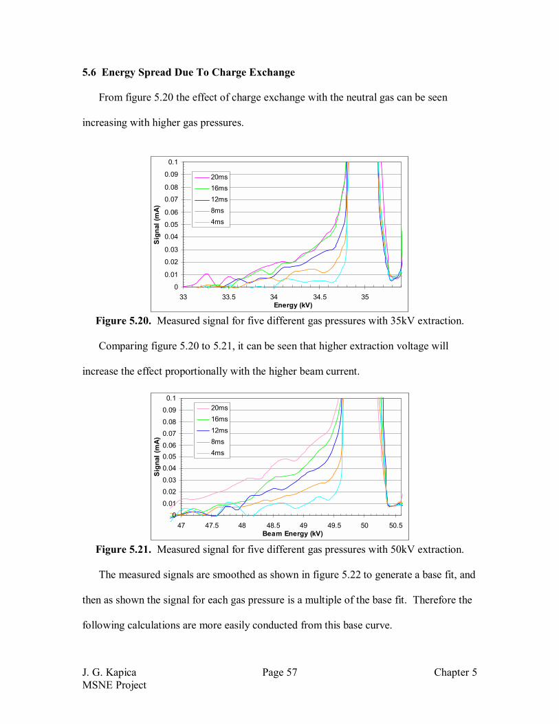
5.6 Energy Spread Due To Charge Exchange

From figure 5.20 the effect of charge exchange with the neutral gas can be seen

increasing with higher gas pressures.

0

0.01

0.02

0.03

0.04

0.05

0.06

0.07

0.08

0.09

0.1

33 33.5 34 34.5 35Energy (kV)

Sign

al (m

A)

20ms16ms12ms8ms4ms

Figure 5.20. Measured signal for five different gas pressures with 35kV extraction.

Comparing figure 5.20 to 5.21, it can be seen that higher extraction voltage will

increase the effect proportionally with the higher beam current.

00.01

0.020.03

0.040.050.06

0.070.08

0.09

0.1

47 47.5 48 48.5 49 49.5 50 50.5Beam Energy (kV)

Sign

al (m

A)

20ms16ms12ms8ms4ms

Figure 5.21. Measured signal for five different gas pressures with 50kV extraction.

The measured signals are smoothed as shown in figure 5.22 to generate a base fit, and

then as shown the signal for each gas pressure is a multiple of the base fit. Therefore the

following calculations are more easily conducted from this base curve.


0

0.01

0.02

0.03

0.04

0.05

0.06

0.07

0.08

0.09

0.1

33 33.5 34 34.5 35Energy (kV)

Sign

al (m

A)

16ms12ms8ms1.5 x FitFit0.5 x Fit

Figure 5.22. Smooth curves fitted to the 35kV measured signal. The curves above and

below the fit are simply multiples of the base fit showing how gas pressure is proportional to measured signal.

The dashed line in figure 5.23 shows the value as predicted using 1/R2 gas density

model. The important factor here is to demonstrate that the approximate magnitude of

energy spread due to charge exchange is in the predictable range. The difference

between the actual signal and calculated model is most likely due to an inaccurate model

for the neutral gas density in the gap.

00.010.020.030.040.050.060.070.080.090.1

33 33.5 34 34.5 35Energy (kV)

Sign

al (m

A)

12msFit1/R2 model 8mT

Figure 5.23. Actual signal compared to fitted curve and predicted curve using a 1/R2 gas

density model.


In order to develop a better fit between the model and actual measured signal, gas

density is found by starting with the measured signal and using the same method in

reverse shown in figure 5.24.

1E+12

1E+13

1E+14

1E+15

0.00 0.05 0.10 0.15


Neut

ral G

as D

ensi

ty (c

m-3

)1/R2 model

Calculated f rom measurement

Figure 5.24. Calculated (from measured signal) gas density shown versus 1/R2 model

gas density. Gas density axis in this graph is shown in log scale. 5.5 Conclusions

The energy spread of the plasma source beam is less than 1% for these extraction

voltages, and the component resulting from charge exchange is in fact much less than

initially expected. Consequently, charge exchange does not present a significant

problem for the overall beam quality. A useful product of this set of experiments is a

neutral gas density profile for the multi-beam grid.

Jonathan Kapica Page 60 Chapter 6 MSNE Project

6. References and Acknowledgements Baca, D., et al. Fabrication of Large Diameter Alumio-Silicate K Sources. Proceedings

of the Particle Accelerator Conference. 2003. Chacon-Glocher, E., Studies in High Current Density Ion Sources for Heavy Ion Fusion

Applications. Ph.D. Dissertation, University of California at Berkeley, 2002. Forrester, T.A., Large Ion Beams, Fundamentals of Generation and Propagation. John

Wiley & Sons, 1978. Humphries, S. Jr., Charged Particle Beams. John Wiley & Sons, 1990. Kwan, J.W., et al. Development of High Current Density Surface Ionization Sources for

Heavy Ion Fusion. Proceedings of the Particle Accelerator Conference. 2001. Westenskow, G.A., et al. High Current Ion Source Development for Heavy Ion Fusion.

2003. Wollnik, H., Optics of Charged Particles. Academic Press, 1987

I would like to thank the following for their invaluable supervision, guidance and

assistance:

LBNL: Dr. Joe Kwan, David Baca, Will Waldron

LLNL: Dr. Glen Westenskow, Robert Hall, Gary Freeze

UCB: Prof. Per Peterson, Prof. Ka-Ngo Leung

Additionally, I am grateful to the Lawrence Berkeley National Laboratory for

financial support and use of equipment and facilities making this all possible.

studies in ion source development for application in heavy

Documents