STUDENT RESEARCH PAPERS VOLUME 28 PART 1 

REU DIRECTOR UMESH GARG, PH.D. 

2017 NSF/REU

RESEARCH EXPERIENCE FOR UNDERGRADUATES

IN PHYSICS

Student Research TitlePage No.

Joseph Arroyo Illinois Institute of TechnologyAriella Atencio Rutgers State University of New JerseyConnor Bagwell University of Notre Dame

Julie Butler Erskine CollegeBridgette Davey Monmouth CollegeIliana De La Cruz St. Mary's UniversityLauren Delgado Vassar CollegeCecilia Fasano University of Notre DameWilliam Feltman Adrian College

James Frisby University of DallasEmmanuel Garcia University of Puerto Rico MayaJazmine Jefferson University of Kansas

David Kalamarides University of Notre DameMichael Kurkowski University of Notre DameKeenan Lambert Chicago State UniversityJoseph Levano University of Notre Dame

REU Student Research Papers – Summer 2017University of Notre Dame – Department of Physics

Testing HECTOR's Efficiency Post Collimator Addition

1

Studies of Electron Reconstruction for the Track Trigger Upgrade for the HL-LHC

11

MicroMegas Design 141

Developing an Electron Beam Heater for Scanning Tunneling Microscopy

41

Accelerator Mass Spectrometry Radiocarbon Dating: Refining the Procedure at the University of Notre DameRotational Analysis of Beryllium Isotopes Using JISP16 and Daejeon16 Interactions

21

31

Energy Resolution Difficulties of the Deep Underground Neutrino Experiment

91

Calculating Electron Drift Velocity & Completing Components of ND Cube

59

PIXE and XRF Analysis of Roman Denarii 71

Experimental Determination of the Angular Acceptance of the STrong: Gradient Electromagnetic Online Recoil Separator for Capture Gamma Ray Experiment (St. George) and Observation of Quadrupole Field Reproducibility

81

Analysis of Colonial Paper Currency 127

Effects of Summer Camp on Participants' Affective Views of Science

49

The use of RF carpets in Helium gas 131

Commissioning of a Faraday Cup for the Solenoid Spectrometer for Nuclear Astrophysics (SSNAP)

101

111

Determining the Effect of Stellar Evolution on Carbon Abundances

121

Identification of candidate metal-poor stars from the HK survey by pruning with the Gaia DR-1 data release

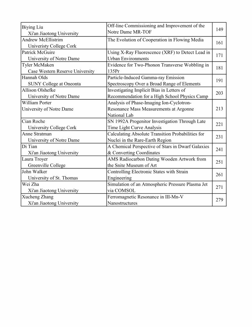
Biying Liu Xi'an Jiaotong UniversityAndrew McEllistrim Univeristy College CorkPatrick McGuire University of Notre DameTyler McMaken Case Western Reserve UniversityHannah Olds SUNY College at OneontaAllison Olshefke University of Notre DameWilliam PorterUniversity of Notre Dame

Cian Roche University College CorkAnne Stratman University of Notre DameDi Tian Xi'an Jiaotong UniversityLaura Troyer Greenville CollegeJohn Walker University of St. ThomasWei Zha Xi'an Jiaotong UniversityXucheng Zhang Xi'an Jiaotong University

Ferromagnetic Resonance in III-Mn-V Nanostructures

279

SN 1992A Progenitor Investigation Through Late Time Light Curve Analysis

221

Calculating Absolute Transition Probabilities for Nuclei in the Rare-Earth Region

231

A Chemical Perspective of Stars in Dwarf Galaxies & Converting Coordinates

241

AMS Radiocarbon Dating Wooden Artwork from the Snite Museum of Art

251

Controlling Electronic States with Strain Engineering

261

Simulation of an Atmospheric Pressure Plasma Jet via COMSOL

271

Investigating Implicit Bias in Letters of Recommendation for a High School Physics CampAnalysis of Phase-Imaging Ion-Cyclotron-Resonance Mass Measurements at Argonne National Lab

Evidence for Two-Phonon Transverse Wobbling in 135Pr

Off-line Commissioning and Improvement of the Notre Dame MR-TOFDetector

149

191

203

213

181

The Evolution of Cooperation in Flowing Media 161

Using X-Ray Fluorescence (XRF) to Detect Lead in Urban Environments

171

Particle-Induced Gamma-ray Emission Spectroscopy Over a Broad Range of Elements

Testing HECTOR’s Efficiency Post Collimator Addition

Joe Arroyo

Advisor: Anna Simon

2017 NSF REU

Department of Physics, Notre Dame University

1

I. Introduction:

Various stellar nuclear processes have been widely accepted as being responsible for the creation

and relative abundances of nuclides observed in the solar system and distant stars (Burbidge et al, 1957).

The various burning stages a star undergoes throughout its lifetime are sufficient for the production of all

nuclides up to iron. The decrease in binding energy per nucleon of higher mass nuclides prevents further

fusion from maintaining hydrostatic equilibrium between gravity and the inner core processes (Bradley

W. Carroll, Dale A. Ostile, 2017).

From this point, neutron capture and subsequent decay accounts for many of the heavier stable β−

nuclides. This is broken down into two processes that differ by the timescale of neutron captures. Stellar

environments may be dense and hot enough to allow for neutron capture that occurs on time scales longer

than the half life of the unstable nuclide that receives the neutron. This is considered slow neutron capture

and is given the alias the s-process, as the now nuclide will on average decay before another A )( + 1 β−

neutron is captured. In an even more virulent environment, neutrons may bombard nuclides at a rate that

is faster than the beta-decay rate. This rapid neutron capture is aptly named the r-process, and subsequent

decays from the end process neutron rich isotope fill in the stable larger mass number nuclides. Bothβ−

of these processes do extremely well predicting the abundances of these nuclides through stellar

modelling. (F. Kappeler et al, 2010 & M. Mumpower et al,, 2015)

With neutron rich nuclides well accounted for, there still remains few proton rich nuclides with

extremely low abundances. These nuclides are effectively “blocked” by stable nuclides preventing β−

decay to provide a pathway for creation of these rare stable isotopes. As such, a new process must be used

to create a model that both forges these nuclides and predicts their relative abundances accurately. A

potential candidate is the p-process, sometimes also referred to as the -process. This is the process by γ

2

which, given a high enough flux of gamma rays, photodisintegration allows for the destruction of

nucleons that carve a pathway to the rarer isotopes. Products of the s-process are thought to be the seed

nuclides for the p-process. Supernovae are the proposed environment for the these seeds due to the large

flux of gamma rays. If supernova were not already difficult enough to model, now all relevant

information to the p-process must be taken into account in complex network calculations to arrive at

proper relative abundances.

Assisting in an experiment to measure the desired characteristics of certain seed nuclides to feed

into these network calculations was the main focus of this project. Cross-section measurements of the

channel for Pd, Cd, and Cd were taken during a one week run with a proton beam atp, )( γ 102 108 110

Notre Dame’s Nuclear Science Lab (NSL) using the FN 10MV Tandem Van de Graaff Accelerator. The

High Efficiency TOtal absorption spectrometeR (HECTOR) was used to measure the gamma rays of

interest. Part way through the experiment, a tantalum collimator was added to allow for the acquisition of

a tighter beam spread and for ease of beam tuning. With the addition of this new component to HECTOR,

the efficiency of the high efficiency detector is affected and the effect is unknown. Calibration runs were

taken with Co with and without the collimator, as well as a known resonance of Al. The task 60 p, )( γ 27

during the NSF Notre Dame Physics REU was to analyze this data to determine the effect of the

collimator on HECTOR’s efficiency.

II. Experimental Methods:

The FN 10MV Tandem Accelerator was used to accelerate a beam of protons towards the targets

of interest. A series of bending magnets, quadrupole magnets, and Einzel lenses are tuned to keep the

beam current on target and as tight as possible. As the energy of the proton beam is changed throughout

the experiment, these must be adjusted to keep the beam tune as tight and on target as possible.

3

The beam was incident upon targets located at the center of HECTOR. HECTOR measures the

gamma rays of interest using 16 4x8x8 inch NaI(Tl) scintillating crystals, each equipped with two

photomultiplier tubes (PMT). The segments are arranged to form a cubic array surrounding the target.

Energy deposited in each crystal is recorded individually during the experiment and summed up to form

one complete spectrum for analysis. This summing procedure requires each PMT to be properly gain

matched and calibrated offline in order to make sure gamma ray energies are consistent between each

PMT and appear in the proper location on the energy spectrum. The summing of these component

spectrums into one sum spectrum allows for nearly steradian coverage of emitted gamma rays with π4

high efficiency.

The measured gamma rays were products of the reactions on Pd, Cd, Cd, p, )( γ 102 108 110 27

Al, targets as well as calibration runs with Co. Following the week of beam time in the NSL, more data 60

was taken to ensure proper spectrums for Co due to inconsistent set up of HECTOR between 60

collimator and no-collimator runs. The inconsistency was different trigger thresholds between runs. This

difference in triggering thresholds caused different amounts of the low energy portion of the sum

spectrum to be suppressed, causing unwanted artifacts during the analysis of the data.

III. Simulations:

To ensure that the experimental results are consistent with what is expected, Geant4 was used to

simulate HECTOR with and without the collimator. Geant4 is used to simulate the passage of particles

through matter. For these simulations, gamma rays are sent through the simulated HECTOR and have a

chance to be absorbed by the NaI(Tl) crystals and recorded in the output sum spectrum.

4

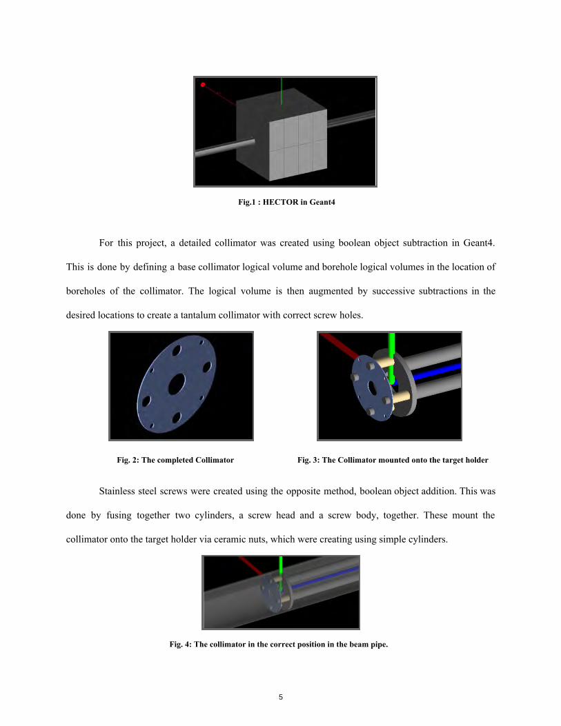
Fig.1 : HECTOR in Geant4

For this project, a detailed collimator was created using boolean object subtraction in Geant4.

This is done by defining a base collimator logical volume and borehole logical volumes in the location of

boreholes of the collimator. The logical volume is then augmented by successive subtractions in the

desired locations to create a tantalum collimator with correct screw holes.

Fig. 2: The completed Collimator Fig. 3: The Collimator mounted onto the target holder

Stainless steel screws were created using the opposite method, boolean object addition. This was

done by fusing together two cylinders, a screw head and a screw body, together. These mount the

collimator onto the target holder via ceramic nuts, which were creating using simple cylinders.

Fig. 4: The collimator in the correct position in the beam pipe.

5

IV. Analysis:

Analysis of the simulated and experimental data was done using C++ and ROOT, a robust object

oriented data analysis framework. To determine the efficiency of the detector, the area under the sum

peak of interest must be calculated. This involves elimination of background counts that may bloat the

counts of the sum peak and elimination of the Compton Continuum that may skew the sum peak.

Background elimination was achieved by taking background runs near the time of the runs of

interest for time lengths sufficient enough to ensure good statistics. From there, scaling of the background

was done either by amplitude of the low energy regime in the spectrum or by total recorded charge from

the experiment. Amplitude scaling was done for the calibration sources, whereas the resonance was scaled

by total recorded charge. Once scaled, subtraction of a background spectrum from a sum peak spectrum is

a simple exercise.

Fig. 5: Background subtraction and comparison with a simulated spectrum

Compton Continuum elimination was achieved by creating a fitting function that first fits a

gaussian on the tail end of the sum peak to ignore most of the lower energy Compton component. After

6

this fit has converged, the best fit for the standard deviation is used as an estimate for the energy width of

the secondary fitting routine. This routine fits a linear background, representative of the Compton

contribution, and a gaussian atop this background, representative of the actual sum peak, over a σ± 3

region about the first fits sum peak energy. Once this fit has converged, the linear background is

subtracted and the histogram’s sum peak is integrated over this region to find the number of counts

contained in the sum peak.

Fig. 6: fitting procedure for an Al sum peak resonance. 27 Green shows the initial rough gaussian fit, red is the gaussian and linear background fit, and magenta is the linear background to be subtracted before sum peak integration

An expected value for the total counts must also be calculated to get the efficiency of these runs.

For calibration data, this is done by looking at the last known activity measurement and using the half life

to calculate the activity of the source the day of the measurements. For the resonance runs, using the

expected sum peak yield, the efficiency can be shown to be as follows,

ε = Aγ

ω nγ 2λ2

where is the efficiency, is the sum peak yield, is the de Broglie Wavelength of the ε Aγ = N source

N sumpeak λ

beam, is the resonance strength, and is the stopping power of the target material (Christian Iliadis, ωγ n

2007).

7

V. Results and Discussion:

The simulated spectra are in a very good agreement with the experimental data. When more

closely examining individual sum peaks, it appears that the standard deviation of the simulation does not

quite match the experimental data. This can be adjusted by creating a more accurate functional form for

the function within the Geant4 simulation itself, which generates the spread about sum peaks as aσ

function of the energy of the sum peak. While this slight difference was not a hindrance to the analysis of

this project, it is an area of improvement for the simulation as a whole.

Fig. 7: Simulation vs. Experimental Al resonance. 27 There is a slight difference between the spread of these sum peaks

The change in efficiency between collimator and no collimator for simulation and experiment

agrees very strongly. This shows that the addition of the collimator within the simulation was

implemented successfully and that there is a good handle on the expected drop in efficiency

experimentally, allowing cross-section data that was taken post-collimator addition to be analyzed with

confidence.

8

Fig. 8: Efficiency for cobalt (left cluster) and aluminum (right cluster) for simulated and experimental sum peaks.

VI. Conclusion:

The addition of the collimator was successfully implemented and the efficiency calculations

between simulation and experiment match strongly. The sources of error on Co calibration runs are 60

essentially negligible. The error bars on the Al data arise from propagation of error in calculation of the 27

resonance strength from parameters in the efficiency equation. Given the errors, the agreement is well

within the discrepancy between most experimental and simulated data. The two outliers with .4%± 0

higher efficiency resulted from simulating a Co source without the beam pipe in HECTOR. This 60

discrepancy is most likely due to a difference in vertical offset of sources between experiment and

simulation. This can be accounted for in the geant for simulation, but that was just outside the allotted

time for this project.

This will be useful for analysis to come on cross-section measurements that were taken for p, )( γ

channels. Not only was the analysis and simulation improvement a success, it also revealed a few points

of improvement within the simulation that may be a component to future REU projects.

9

VII. References:

1. K. Margaret Burbidge, G. R. Burbidge, William A. Fowler, F. Hoyle. Synthesis of Elements In

Stars. Reviews of Modern Physics, 29-4 (1957).

2. Bradley W. Carroll, Dale A. Ostile. Introduction to Modern Astrophysics, An, 2nd Edition. Pearson (2007).

3. F. Kappeler, R. Gallino, S. Bisterzo, Wako Aoki. The s-Process: Nuclear Physics, Stellar Models,

Observations. arXiv:1012.5218v1 (2010).

4. M.R. Mumpower, R. Surman, D.-L. Fang, M. Beard, P. Moller, T. Kawano, A. Aprahamian. The impact of individual nuclear masses on r-process abundances. arXiv:1505.07789v1 (2015).

5. Christian Iliadis. Nuclear Physics of Stars. Wiley-VCH Verlag GmbH & Co. (2015).

10

Studies of Electron Reconstruction For the

Track Trigger Upgrade For the HL-LHC

Ariella Atencio

2017 NSF/REU Program

Physics Department, University of Notre Dame

Advisors:

Professor Kevin Lannon

Professor Mike Hildreth

26 July, 2017

11

The world’s largest and most powerful particle accelerator, the Large Hadron Collider

(LHC) has been running since September of 2008. The LHC consists of a 27 kilometer ring of

superconducting magnets with many accelerating structures to boost the energy of the particles

along the way. Inside the accelerator, two high energy particle beams travel close to the speed of

light and are then collided. The two beams travel in opposite directions in separate beam pipes

kept at ultrahigh vacuum. All of the controls for the accelerator are kept at the CERN Control

Centre, where the beams inside LHC are made to collide at four locations corresponding to the

four particle detectors which are ATLAS, CMS, ALICE, and LHCb. [1]

The LHC smashes groups of protons together near the speed of light. Many of these

collisions are just glancing blows but some will be “head on” very energetic collisions. Some of

this energy from the collisions is turned into mass in the form of previously unobserved,

short-lived particles. This could give clues into how nature behaves at a fundamental level. The

CMS is a particle detector and high performance system designed to see a wide range of particles

and phenomena produced in high-energy collisions in the LHC, it is particularly good for

detecting and measuring muons. The detector has many layers to it, each of which measures all

of the different particles, and this data is used to build a picture of events in the heart of the

collision. This data is used by Scientists to help answer questions such as: What is the Universe

made of? What gives everything substance? The CMS will also be used to measure the

properties of previously discovered particles with incredible precision. [2]

There are several layers to the CMS detector. The tracking layer measures charged

particles and outside that there are the calorimeters for measuring energy and the muon system

for identifying muons. A very strong magnet is used to measure momentum. The higher a

12

charged particle’s momentum, the less its path is curved in the magnetic field. The large magnet

allows many layers of muon detectors to use the magnetic field so the momentum can be

measured both inside and outside the coil. The “S” in “CMS” stands for solenoid, which refers to

the coil of superconducting wire that creates a magnetic field when electricity flows through it.

When a collision happens, a particle emerging from the collision first encounters the tracking

system which is made up of silicon pixels and silicon strip detectors. This accurately measures

the positions of passing charged particles to reconstruct their tracks. Charged particles follow

spiral paths in the magnetic field. The curvature of the path reveals their momenta. The particles

flying out of the collisions have such high energies that it takes big distances to absorb them. The

bigger the detector, the more measurements can be taken in “tracking” the particle, meaning

more accuracy in the momentum calculation.

The LHC will soon get an upgrade known as the High-Luminosity Large Hadron Collider

(HL-LHC). This upgrade, which should be finished by 2023, will increase luminosity and

therefore collisions rate by a factor of ten.. Since the LHC is getting an upgrade, the CMS will

also need an upgrade to accommodate the larger number of collisions occurring. If the CMS

cannot accurately detect all of the interesting collisions, then the HL-LHC upgrade will be

useless. In order to get the most out of this increase in collision frequency, the CMS will need to

be able to quickly and accurately sift through the large amounts of data. The trigger (which

decides what data to keep) in the CMS currently can’t use the tracking information, but using the

tracking information in the trigger would be very helpful with managing the higher collision

rates. The track trigger we have been working on would work great for muons, but not so much

13

for electrons. Although we know in principle how to make the trigger work well for electrons,

the struggle is in making a practical algorithm that can work in microseconds.

Efficiencies of electrons is significantly worse than muons, with muons at least 95%

efficient and electrons sometimes dropping as low as 80% efficient. This is due to

Bremsstrahlung radiation and electron scattering. Bremsstrahlung radiation can lead to large

discrete energy loss. It is caused by acceleration due to interaction with coulomb field of nuclei.

It is the dominant energy loss mechanism for electrons and positrons. Also, light particles like

electrons are more deflected by their interaction with atoms in the detector than heavier particles

like muons, which is known as electron scattering. Because of the radiation and scattering, stubs

aren’t where the algorithm expect them to be. So the question is raised, can we recover any of

those electrons that aren’t reconstructed and improve efficiency? In order to accomplish this we

need to find patterns in the missed electron tracks and use them to redesign the tracking

algorithm.

A track is a parametric representation of a charged particle’s trajectory. Charged particles

follow a curved trajectory in a magnetic field due to the Lorentz force. The radius of curvature is

inversely proportional to momentum. So, we need to measure the radius of curvature, but radius

measurement implies knowing where the particle is at several points along its trajectory.

Tracking detectors use ionization of the detector material to register the positions where the

particle passes through the detector, allowing a reconstruction of the particle trajectory. The

tracking algorithm is explained in detail in reference [3].

The motivation of this project is that electron tracking is worse because of

Bremsstrahlung radiation, which causes them to lose momentum, curves more, and as a result

14

doesn’t match the expected pattern. In other words, we can’t reconstruct electrons that brem

because their stubs don’t end up where you’d expect them to be based on a particle that isn’t

radiating and losing momentum. We tried to study this further by looking at how far the actual

electron stubs are away from their expected positions. To check the inaccuracy of the electron

tracking, a simulation was used to calculate the actual tracking particle path (giving the location

of where the stubs should be) which was compared to where we see the stubs. The main

coordinates we use in this comparison are and z. is the difference between the actualrΦΔ rΦΔ

tracking particle position radius times the angle and the measured stub radius times the angle.

is the difference along the path of the CMS detector between the actual tracking particle andzΔ

the measured stub. These equations are given in the following equations.

r = √x2 + y2 The variables used in these equations are described as follows:rctan( )Φ = a x

y x and y are the x,y-coordinates of the stub inh(η)zexp = r * s + z0 r is the radius of the stub. is the angle of the stub in the x,yΦ

R = pt1.14 plane, is the expected z-coordinate of the stub, eta is thezexp

pseudo-rapidity, and is the z value for the point along the trackrcsin( )Φexp = a r2R + Φtp z0

zΔ = zstub − zexp closest to the center. R is the radius of the track’s curvature, ispt rΦ Φ )Δ = r * ( − Φexp the transverse momentum of the tracking particle. is the angleΦtp

in the x,y plane of the tracking particle. is the expected phiΦexp value of the tracking particle. is the difference between thezΔ z-coordinate of the stub and the expected z-coordinate. is therΦΔ difference between phi and the expected phi times r.

This approach was validated by looking at muons, whose actual paths were well-represented by

their stubs.

15

Figure 1.1: Left: for 100,000 events of Muons, in layer 6. Right: for 100,000 eventsrΦΔ rΦΔ

of Electrons, in layer 6.

In histograms for the of muons, they tend to stay close to zero in all layers and for bothrΦΔ

positive and negative muons. For the same histograms of electrons, however, increasesrΦΔ

with each layer, with tails going into the positive or negative direction depending on the charge

of the electron.

Figure 1.3: On the left, in layer 4 for negative muons. On the right, in layer 4 forzΔ zΔ negative electrons.

16

In , both muons and electrons have values in the expected window. This makes sense becausezΔ

Bremsstrahlung radiation only affects the curvature of the tracking particle path in the rΦΔ

plane, not in the z direction which the magnetic field does not affect.

One known issue with electrons is that the bremsstrahlung photons can pair convert,

creating additional electron-positron pairs that also leave stubs. When a histogram for the

number of stubs per event was made, it was discovered that some events had as many as fifty

stubs in one track. This was surprising because only about six stubs were expected for each track

(one for each layer of the CMS). Also, it was pointed out that the more stubs an event has, the

more likely the track is to not be found. So events where the electron track is not reconstructed

can be confusing because there could be many stubs. To try to remove that confusion, we focus

on only the nearest stub for the rest of the discussion.

Figure 1.4: On the left, the number of stubs per event for single track negative electrons with 100,000 events. On the right, the number of stubs per event for single track negative electrons with 100,000 events when the track was not found.

17

Further investigation revealed that in the inner three layers, the stubs are mostly where

they're expected, while after that, they are more and more likely to be far away. So the problem

is to find the stubs when they're far away from where they're supposed to be.

Figure 1.5: Histograms of for single track negative electrons in 100,000 events. These arerΦΔ the data for the stub with the smallest per event when the track was not found. EachrΦΔ histogram represents a different layer of the CMS.

In two-dimensional histograms comparing the of one layer to the next, we see arΦΔ

correlation across layers.

18

Figure 1.6: Two-dimensional histograms of . To the left: layer 3 on the x-axis versus layerrΦΔ 4 on the y-axis for single track negative electrons in 100,000 events. In the center: Layer 4 vs Layer 5, and to the right: Layer 5 vs Layer 6This is the data for the stub with the smallest rΦΔper event when the track was not found.

When the stubs are off target, they’re off target in a way that is correlated between layers. So, if

someone told you how far off you are in layer 3, you should be able to determine how far off the

next stub will be in layer 4. Perhaps, this pattern could be used to re-write the tracking algorithm.

Figure 1.6: On the left, a cartoon depicting the current setup for the tracking algorithm. On the right, a cartoon representation of a hypothetical tracking system that could correct for Bremsstrahlung radiation.

Rather than simply widening the window of possibilities for the next stub, perhaps the tracker

could use the most recent stub to change the position of the window so that it might look more

19

accurately for the next stub. If the window is more accurately positioned, more electron tracks

could be found even if they Bremsstrahlung radiate.

The algorithm suggested above would definitely work in theory, but it may not be

practical. The next steps in this research will be to explore whether there is a feasible way to

implement this algorithm that would work for the trigger.

References

[1] “The Large Hadron Collider” CERN, Accelerating Science

http://home.cern/topics/large-hadron-collider

[2] Lucas Taylor “What is CMS?” 2011-11-23, http://cms.web.cern.ch/news/what-cms

[3] Ben Cote and Patrick Shields “Feasibility Studies For the Proposed CMS L1 Track Trigger

Upgrade” August 5th, 2016

20

Accelerator Mass Spectrometry Radiocarbon Dating:

Refining the Procedure at the University of Notre Dame

Connor Bagwell

University of Notre Dame, Department of Physics

Research Experience for Undergraduates

28 July 2017

Principal Investigator:

Professor Philippe Collon

Coauthors:

Tyler Anderson, Adam Clark, Austin Nelson, Michael Skulski, Laura Troyer

21

Abstract

Accelerator Mass Spectrometry (AMS) is a highly sensitive technique for measuring trace isotopic

ratios, making it perfectly suited for radiocarbon dating. AMS radiocarbon dating deviates from decay activity

measurements, which measure isotopic decay activity in a sample over time and are unable to measure

extremely low isotopic abundances, such as 14C to stable carbon (10-12 or lower), without taking prohibitively

large samples or periods of time. AMS uses minute sample sizes, making the technique much less destructive.

The use of an entire accelerator system to discriminate from background is orders of magnitude more

sensitive in small samples than both decay activity measurements and traditional mass spectrometry methods

[1]. AMS measures the specific number of events of 14C detected from the beams of both unknown

graphitized carbon and known standards and calculates the number of total carbon ions from the beam current.

The isotopic concentration of the sample is then calculated from this set of measurements, and the measured

concentrations are calibrated with known historical concentration data, producing date ranges and associated

probabilities for that sample [2]. The Snite Museum of Art provided the AMS group with samples from five

wooden art pieces as the unknowns to be graphitized and measured.

The Technique: Accelerator Mass Spectrometry

Accelerator Mass Spectrometry (AMS) is referred to as the “needle in the haystack method” because it

deals with detecting trace isotopes amongst a spread of more abundant isotopes. These isotopes, often

radioactive, are measured in ratios of 10-10 to 10-16 [3]. In the case of radiocarbon dating, 14C is the isotope of

interest and has an isotopic ratio to stable carbon of 10-12. These less abundant isotopes require entire

accelerator systems to discriminate from background noise and unwanted contaminations, since accelerators

offer numerous, highly sensitive adjustments that can be tuned to detect only the nuclide of interest.

AMS begins with some sample to be measured, inherently comprised of many different elements and

isotopes, and attempts to measure the current isotopic ratio of interest. The technique incorporates several

22

methods of filtration to differentiate between desired counts and background noise. The 11 MV FN tandem

accelerator and AMS beamline at the University of Notre Dame’s Nuclear Science Laboratory (NSL) was

used for these experiments. The FN incorporates several magnets, an electrostatic analyzer, and a Wein filter

to reduce isobaric contaminants, making it suitable for measuring several long-lived isotopes [4].

AMS applications are many and diverse. Nuclear forensics, for example, measures the distribution of

isotopes for the elements known to be used in nuclear weaponry manufacturing or as the byproduct of nuclear

bomb reactions [5]. There exists a natural distribution of unstable isotopes, and if the measured distribution is

found to be significantly different than that natural distribution, governments can identify those parties in

violation of disarmament treaties. Additionally, nuclear reactor accidents can be studied using AMS to

discover future warning signs and hidden failures [5]. In biomedical research, the highly sensitive

measurements using AMS are used to detect the effects of micro-doses of man-made radioisotopes during

tests for new drugs [5]. In archaeology, calcium dating is an attractive frontier of AMS research, which would

allow researchers to date events beyond the human-scale of activity, measured by radiocarbon dating [5].

Further applications extend to astrophysics, glacial changes, atmospheric data, and numerous others.

AMS Radiocarbon Dating

One of the most useful applications of AMS is radiocarbon dating, which relies on the carbon life

cycle. The atmosphere contains a broad mixture of elements, of which carbon is the fourth most abundant.

The most abundant element is nitrogen, of which most is stable 14N. Thermal neutrons created from cosmic

ray interactions collide with 14N to create 14C, as shown in the following reaction:

Figure 1 A nitrogen-14 atom reacts with an incoming neutron in the atmosphere to produce carbon-14 and a proton.

The 14C eventually beta decays back into 14N, releasing an electron and an antineutrino.

23

Carbon dioxide in the air, containing a ratio of 14C to stable carbon isotopes, is absorbed by plants,

undergoing isotopic fractionation. Isotopic fractionation, stated simply, says that heavier isotopes of an

element will undergo chemical processes slower than lighter isotopes [6]. During photosynthesis, for example,

there is a higher uptake of 12C than 13C. The carbon then either continues to build in the plant or is eaten by an

animal or other consumer. The animal not only takes in carbon by consuming, but also by breathing. The

moment of death of an organism is the point at which the radiocarbon clock starts; this is time zero. The

organism is no longer taking in any new carbon and therefore equilibrates with the environment.

The idea is that while alive, the organism, be it a tree, a bug, or an animal, has roughly the same

isotopic ratios of carbon as the atmosphere, to within a correction [1]. At time zero, the organism is no longer

equilibrating with the environment, and its distribution of carbon isotopes will be set, while the radioactive

carbon isotopes will begin to decay away from this atmospheric concentration [1]. Using the exponential

decay law and a thorough set of known historical atmospheric concentration data, one can calculate the age of

the sample in question.

A set of historical concentration data has been collected and published by the scientific community for

reference and use in calibration curves for dating purposes [5]. The input to the calibration is the measured

concentration of 14C to stable carbon (12C and 13C), in the form of units called fraction of modern (F14) [7]. F14

refers to the fraction of 14C at present to the 14C on 1 January 1950, the universally accepted “modern”

concentration of 14C to stable carbon [6]. Measurements made since then have added to the data set past

“modern” levels, and precise measurements of samples from trees with well-defined ages, given by their tree

rings, allow this precise atmospheric concentration data to reach back well past 1950 [6]. The calibration

software used in these experiments was OxCal, the radiocarbon calibration tool developed by the Oxford

Radiocarbon Accelerator Unit [2].

24

Graphitization: From Carbon Based Life to Coal

The most effective form of carbon to use in an accelerator system is pure graphite [7]. Graphitization is

the process of forming ideally pure graphite from a source of carbon. In the case of this experiment, the

carbon came from the wood shavings from internal samples of the art pieces. The process can be broken down

simply into the following steps: treatment of the iron matrix, combustion and transfer of the sample, reduction

of carbon dioxide to carbon monoxide, and graphitization of carbon monoxide to graphite. The pressure

versus time chart of the process is outlined in Figure 2.

I. Treatment of the Iron Matrix:

The carrier for the graphite is an iron matrix, 2-3 mg of iron powder. The iron is oxidized at atmosphere

using an oven at 900 C, then baked at vacuum, each for 30 minutes. The iron is then treated twice with 12.3

psi of hydrogen, 15 minutes a piece, at 815 C, until the iron is brilliantly light in color, as shown in Figure 3.

A liquid nitrogen cold finger is applied to the system to draw out any water vapor.

II. Combustion and Transfer of the Sample:

Combustion of the sample releases carbon

dioxide, which is captured and chemically

reduced to graphite. A measured 3.6 mg of wood

sample is combusted in a quartz tube for an hour with 480 mg of copper oxide. The copper oxide is the source

of oxygen in the combustion which is heated to 900 C. The leftover oxygen produced by the copper oxide

Figure 2 The standard pressure reading throughout the graphitization process, including readings from two pressure gauges: the combustion tube and the iron treatment and graphitization tube.

Figure 3 The iron undergoes two hydrogen treatments, resulting in a lighter and brighter colored iron matrix in the isolated system.

25

reduces back onto the copper until the pressure levels off. The

gas produced by combustion is then transferred through a water

trap of ethanol and dry ice slush mixture, through which water

freezes and carbon dioxide passes. The transfer is made by a

temperature gradient to the graphitization tube, where the

treated iron matrix is sitting. The temperature difference is

created by placing liquid nitrogen over the graphitization tube,

which is cold enough to freeze the carbon dioxide. Once pressures level off, the graphitization tube is sealed

and the carbon is now in dry ice form, as seen in Figure 4. The remaining gases are pumped away before

continuing.

III. Reduction

A ratio of 2.3:1 of hydrogen to carbon dioxide pressure is added to the system. The first stage of

graphitization chemically reduces carbon dioxide to carbon monoxide, by the reaction in Figure 5.

Figure 5 Carbon dioxide and hydrogen gas reduce to carbon monoxide and water.

The oven is set to 915 C, at which point the reduction takes place. The reaction continues for 90 minutes with

the ethanol and dry ice slush mixture on the cold finger. By the end of this process, ideally, the carbon dioxide

will have reduced to carbon monoxide, without creation of methane, and the water will have been trapped in

the cold finger.

IV. Graphitization

In the second stage of graphitization, the following reaction dominates:

Figure 6 Carbon monoxide and hydrogen gas reduce to water and graphite, the latter of which embeds itself into the iron matrix.

Figure 4 From left to right, wood shavings from the artwork, carbon dioxide crystals in the graphitization tube, and carbon dioxide condensed on the sides of the graphitization tube.

26

The oven is set to 600 C and liquid nitrogen is placed around the cold finger to freeze any methane and water

created or residual carbon dioxide. This final stage takes roughly six hours to fully react, during which time

the graphite embeds within the iron matrix. The final product is a black powder comprised of graphite and

iron.

The 11 MV FN Tandem Accelerator

The samples are loaded into aluminum sample holders, called cathodes for the function they serve in

the ion source. The cathodes are then loaded into a forty-cathode wheel, and mounted in the source of

negative ions via cesium sputtering (SNICS) chamber. Cesium is heated to form a gas and coats the

electrostatic plates in the chamber. During heating, the cesium releases its loose electrons, and the cesium

becomes positively charged. The cesium accelerates towards the cathode, collides, and produces singly

charged negative ions of carbon. These carbon ions accelerate toward and past the electrostatic plates coated

in positively charged cesium into the accelerator. The ion’s path is outlined in Figure 7.

The accelerator system sorts first by kinetic energy in the electrostatic analyzer (ESA), requiring the

kinetic energy of an ion of 14C accelerated from the SNICS to pass. The beam is sorted by mass in the SNICS

magnet, using the principle of the Lorentz force. The

particles are accelerated through the main tank and

stripped of electrons using a carbon foil. The carbon

occupies a distribution around the +3 charge state, i.e.,

the carbon ions are missing, on average, three electrons.

So, the beam passes through the analyzing magnet to

select only the +3 charge state. In the target room, the

beam passes through a Wein filter, utilizing the Lorentz

principle and only allowing past the particles with the

Figure 7 The NSL FN tandem accelerator, AMS beamline, filtration techniques, and parallel grid avalanche counter (PGAC) outlined.

27

correct velocity, calculated from the desired charge and mass. The particles finally hit the parallel grid

avalanche counter (PGAC) and ionization chamber, which detect the events of 14C. At this point, AMS

measurements would typically employ an ionization chamber, which forces the beam to collide with a gas

and, on average, take on different charges based on the number of protons within the isotope. This filtration

technique allows one to sort out isobaric contaminations, which would have successfully passed through the

discrimination methods. One major benefit of AMS radiocarbon dating is that 14C does not require this last

filter since its isobar, 14N, cannot form negative ions in the SNICS to begin with.

Data & Conclusion

The results from the data obtained from the 20 July 2017 University of Notre Dame NSL FN tandem

accelerator run are shown in Table I, laid out by museum piece, separated into the multiple graphitizations

produced for each sample. The raw data obtained consisted in part of 14C events and both run-average and

Sample Graphitization Date Probability Run-Averaged Age Range Probability Time-Averaged Age Range

Museum 1 July 6, 2017 95.4% 848 BC - 1085 AD 95.4% 866 BC - 1067 ADJune 28, 2017 79.5% Pre-1893 79.5% Pre-1893

15.9% 1906-1954 15.9% 1906-1954Museum 2 July 2, 2017 32.0% 1664-1787 34.5% 1664-1787

48.0% 1791-1958 50.8% 1790-195815.4% Post-1987 10.1% Post-1990

June 29, 2017 35.1% 1664-1788 34.9% 1664-178851.1% 1789-1958 50.8% 1789-19589.2% Post-1990 9.7% Post-1990

Museum 3 July 8, 2017 16.9% 1957-1962 16.0% 1957-196278.5% 1979-2006 79.2% 1979-2007

0.2% 2008July 8, 2017 95.4% 1882 BC - 265 AD 95.4% 1914 BC - 232 AD

June 20, 2017 95.4% 1199 BC - 914 AD 95.4% 1151 BC - 964 ADMuseum 4 July 10, 2017 95.4% Pre-1655 95.4% Pre-1655

July 1, 2017 43.2% Pre-1669 54.5% Pre-166638.8% 1781-1798 40.9% 1783-179613.5% 1945-1951

Museum 5 July 12, 2017 4.2% 1681-1738 3.6% 1681-17380.2% 1745-1748 0.4% 1755-17620.7% 1750-1763

10.2% 1802-1938 8.8% 1803-193712.5% 1802-1938 13.3% 1952-196267.6% Post-1976 69.4% Post-1976

June 26, 2017 95.4% 1262 95.4% 2241 BC - 477 BC

Table 1 Data collected from the accelerator run made on 20 July 2017 and processed through the OxCal calibration software to output date ranges and associated probabilities for the five pieces of African Art.

Table I: African Art Date Ranges, 20 July 2017

28

time-average beam current, which are used to calculate the raw measured concentration. This concentration is

normalized with our measured standards, giving us a corrected concentration, which, after corrections

outlined in Donahue [8] for isotope fractionation, allows for the calculation of fraction modern. The OxCal

software takes this input, fits the data along its calibration curve comprised of historical isotopic concentration

data, and outputs the calibrated date ranges with their associated probabilities, a product of their “wiggle

fitting” program [2].

Easily seen is the magnitude of error in this data set, rendering the date ranges inconclusive. The intent

of the summer research was to continue improvements upon and refinements to the graphitization process at

the University of Notre Dame. The amount of beam current achieved in July 2017 (101 microamps) was two

orders of magnitude higher than the original attempts at graphitizing wooden samples in the NSL (102

nanoamps). This improvement was brought about by several changes made to the process. The AMS group

doubled the hydrogen treatments to the iron matrix to two, began graphitizing on the same day as the iron was

treated, allowing the oxygen to react with the copper after combustion to reoxidize into copper-oxide,

increasing the duration of transferring gas after combustion, and improving lab discipline regarding note

keeping for future use of information on lab procedures and trials.

This AMS group will further refine the procedure until the NSL is able to replicate significant results in

radiocarbon dating. AMS requires extreme precision and sensitivity in the four principles of AMS defined in

Synal [9] as the suppression of nuclear isobaric ions, suppression of equal mass molecules, provision of

sufficient abundance sensitivity, and establishment of reliable normalization procedure, which are key to any

AMS measurement technique.

Acknowledgements

The REU at Notre Dame is funded by the National Science Foundation. My summer would not have

been possible without the generosity and financial aid of the Department of Physics. In cooperation with

29

ISNAP, JINA-CEE, and Notre Dame physics faculty, the ND AMS group brought this humble author through

the principles of AMS, making me a passable amateur nuclear physicist. Special thanks to the graduate

students Tyler Anderson, Adam Clark, Austin Nelson, and Michael Skulski for showing me how brilliant

Notre Dame graduate students are. To my colleague, Laura Troyer, for learning with me the whole way. And

to my advisor, Professor Philippe Collon, for guiding and encouraging me these last two years.

References

[1] Kutschera, Walter. Applications of accelerator mass spectrometry. International Journal of

Mass Spectrometry, 349-350 (2013) 203-218.

[2] OxCal, Oxford Radiocarbon Accelerator Unit. Radiocarbon Calibration.

https://c14.arch.ox.ac.uk/calibration.html

[3] Litherland, A. E. Ultrasensitive Mass Spectrometry with Accelerators. Annual Review of

Nuclear Particle Science, 1980.30 (1980) 437-473.

[4] Bowers, Matthew R. A Study of 36Cl Production in the Early Solar System. University of

Notre Dame (2013).

[5] Kutschera, Walter; Michael Paul. Accelerator Mass Spectrometry in Nuclear Physics and

Astrophysics. Annual Review of Nuclear Particle Science, 1990.40 (1990) 411-438.

[6] Stenström, Kristina Eriksson; Göran Skog, Elisavet Georgiadou,

Johan Genberg, Anette Johansson. A Guide to Radiocarbon Units and Calculations. Lund

University (2011).

[7] McNichol, A.P.; A.J.T. Jull. Converting AMS Data to Radiocarbon Values: Considerations

and Conventions. Radiocarbon, Vol. 43, 313-320 (2001).

[8] Donahue, D.J.; T.W. Linick, A.J.T. Jull. Isotope-Ratio and Background Corrections for

Accelerator Mass Spectrometry Radiocarbon Measurements. Radiocarbon, Vol. 32, No. 2.

(1990) 135-142.

[9] Synal, Hans-Arno. Developments in accelerator mass spectrometry. International Journal of

Mass Spectrometry 349-350 (2013) 192-202.

30

Rotational Analysis of Beryllium

Isotopes Using JISP16 and Daejeon16

Interactions

Julie Butler

2017 NSF/REU Program

Physics Department, University of Notre Dame

ADVISOR: Mark A. Caprio

July 28, 2017

31

Abstract

Rotational bands emerge in ab initio no core configuration interaction (NCCI) calculations in

several beryllium isotopes. This is shown by rotational patterns in excitation energies, elec-

tromagnetic moments, and electromagnetic transitions as functions of the angular momen-

tum. In order for NCCI calculations to correctly describe the nucleus, the NCCI calculation

must be based on a realistic nucleon-nucleon interaction. The nucleon-nucleon interaction

JISP16 has been previously used to calculate the rotational bands in beryllium isotopes.

However, a new nucleon-nucleon interaction, Daejeon16, has been shown to provide more

accurate ground state energies of light nuclei. This research compares the ability of the

two nucleon-nucleon interactions, JISP16 and Daejeon16, to describe rotational bands of the

beryllium isotopes 7 Be, 8 Be, and 9 Be. For each isotope and interaction, rotational bands

are determined using a range of basis parameters to determine which interaction yields ro-

tational band parameters which most closely match experimental values. Various methods

of extrapolation are used to determine converged values of rotational band parameters.

Introduction

Ab initio no-core configuration interaction (NCCI) calculations are used to identify rota-

tional bands in p-shell nuclei. These rotational bands are identified by rotational patters in

energies, electromagnetic moments, and electromagnetic transitions as functions of angular

momentum.1 NCCI calculations are able to calculate properties of many light nuclei with

masses up to A = 16.2 In order for the NCCI calculation to accurately describe the nucleus,

it must be base on a realistic nucleon-nucleon interaction. Two such nucleon-nucleon inter-

actions are known as JISP16 and Daejoen16. This paper will compare the ability of both

JISP16 and Daejeon16 to calculate the rotational bands in the beryllium isotopes 7Be and

8Be. The dependence of rotational bands on the NCCI calculation parameters hω and Nmax

is also explored. In order to determine the accuracy of each nucleon-nucleon interaction,

rotational band parameters are extracted and compared to experimental results. Various

extrapolation techniques are utilized to attempt to estimate the rotational parameters of

converged calculations for the rotational bands.

32

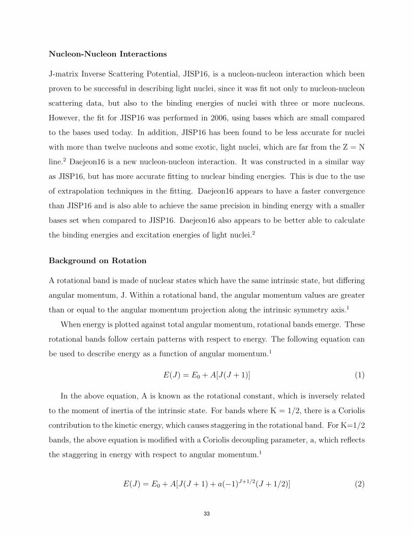
Nucleon-Nucleon Interactions

J-matrix Inverse Scattering Potential, JISP16, is a nucleon-nucleon interaction which been

proven to be successful in describing light nuclei, since it was fit not only to nucleon-nucleon

scattering data, but also to the binding energies of nuclei with three or more nucleons.

However, the fit for JISP16 was performed in 2006, using bases which are small compared

to the bases used today. In addition, JISP16 has been found to be less accurate for nuclei

with more than twelve nucleons and some exotic, light nuclei, which are far from the Z = N

line.2 Daejeon16 is a new nucleon-nucleon interaction. It was constructed in a similar way

as JISP16, but has more accurate fitting to nuclear binding energies. This is due to the use

of extrapolation techniques in the fitting. Daejeon16 appears to have a faster convergence

than JISP16 and is also able to achieve the same precision in binding energy with a smaller

bases set when compared to JISP16. Daejeon16 also appears to be better able to calculate

the binding energies and excitation energies of light nuclei.2

Background on Rotation

A rotational band is made of nuclear states which have the same intrinsic state, but differing

angular momentum, J. Within a rotational band, the angular momentum values are greater

than or equal to the angular momentum projection along the intrinsic symmetry axis.1

When energy is plotted against total angular momentum, rotational bands emerge. These

rotational bands follow certain patterns with respect to energy. The following equation can

be used to describe energy as a function of angular momentum.1

E(J) = E0 + A[J(J + 1)] (1)

In the above equation, A is known as the rotational constant, which is inversely related

to the moment of inertia of the intrinsic state. For bands where K = 1/2, there is a Coriolis

contribution to the kinetic energy, which causes staggering in the rotational band. For K=1/2

bands, the above equation is modified with a Coriolis decoupling parameter, a, which reflects

the staggering in energy with respect to angular momentum.1

E(J) = E0 + A[J(J + 1) + a(−1)J+1/2(J + 1/2)] (2)

33

In NCCI calculations, the many-body Schrodinger equation is formulated as Hamiltonian

matrix diagonalization problem.3 The Hamiltonian is represented with respect to a basis of

antisymmetrized products of single-particle states, typically harmonic oscillator states. Due

to computational limitations, NCCI calculations are carried out in truncated space, defined

by the maximum number of allowed oscillator excitations, Nmax. Convergence to exact results

could be obtained by increasing Nmax. However, computational limitations place limits on

the maximum accessible value of Nmax. Because of this, the calculated results depend not

only on the length parameter b for to oscillator basis function, typically specified by the

oscillator energy hω, but also on the basis truncation Nmax.2,3

Extrapolation Methods

Due to computational limitations, NCCI calculations must be carried out in truncated space.

This limits the convergence of the results. Converged results can be estimated using various

methods of extrapolation. Though these extrapolation methods are still in there formative

stages, two of these methods, exponential extrapolation and infrared extrapolation, are ex-

plored in this paper to estimate the converged energies for the ground and excited states of

the beryllium nuclei.

Table 1: The two extrapolation schemes explored in this research: exponential extrapolation and infrared

extrapolation.

Exponential Extrapolation3 Infrared Extrapolation4,5,6

E(Nmax) = c0 + c1e−c2Nmax ΛUV = [2(Nmax + 3/2)]1/2(h/b(hω))

Converged Energy: c0 b(hω) = hc/[(mN c2)(hω)]1/2

L2(Nmax, hω) = [2(Nmax + ∆Nmax + 3/2)]1/2b(hω)

E(L) = E∞ + a0e−2k∞L

Converged Energy: E∞For each nucleon-nucleon interaction, the optimal UV cutoff can be determined from the

Nmax and hω values that were used to fit the data. The UV cutoff of the JISP16 interaction

was estimated to Ref. [4] to be approximately 800MeV/c, obtained from the fact that the

JISP16 interaction was fit using data obtained from Nmax = 8 and hω = 40 MeV.4 Dajeon16

was fit with data obtained at a hω value of 25 MeV, so its UV cutoff will be lower than the

34

UV cutoff of the JISP16 interaction. UV cutoffs of 550MeV/c and 800MeV/c are explored in

this paper.

Results

NCCI calculations were performed with both the Daejeon16 and JISP16 nucleon-nucleon

interactions using the code MFDn.7,8

Rotational bands become evident in the beryllium isotopes when the energy of the ground

and excited states are plotted as a function of angular momentum, denoted by J. The angular

momentum axis is scaled as J(J+1). Figure 1 shows these rotational plots for the beryllium

isotopes 7Be and 8Be, with the JISP16 interaction.

1/2 3/2 5/2 7/2

J

− 40

− 38

− 36

− 34

− 32

− 30

− 28

− 26

− 24

Energy (MeV)

(a) 7Be JISP16 Natural Parity (P=-)

0 2 4 6

J

− 55

− 50

− 45

− 40

− 35

− 30

− 25

− 20

− 15

− 10Energy (MeV)

(b) 8Be JISP16 Natural Parity (P=+)

Figure 1: Energy eigenvalues obtained for states in the natural parity and unnatural parity spacesfor 7Be and8Be. Energy is plotted as a function of angular momentum, scaled as J(J+1) to allowfor identification of rotational energy patterns. Square symbols represent band member candidates.Plots shown here were made with results obtained using a hω of 20MeV and an Nmax value of 8.

The yrast band for Beryllium-7 and Beryllium-8 are shown above in Figure 1. The yrast band

generally connects the lowest energies with respect to different angular momentum values.

As shown above, the yrast band of Beryllium-7 is staggered, indicating that is has a non-zero

Coriolis decoupling parameter, which will be used later in determining the rotational band

parameters.

Candidate band members are identified visually using the plots shown above. The band

35

members are confirmed through analysis of electromagnetic quadruple moments; members

of the same rotational band have electromagnetic quadruple moments of similar magnitude

and sign. For example in the Beryllium-7 plots shown above in Figure 2, for both JISP16

and Daejeon16, the first J=5/2 state visually appears to be the band member. However, the

second J=5/2 state has an electromagnetic quadruple moment which more closely matches

the moments of the other three candidate band members. Therefore, the second J=5/2 state

was chosen as the band member for Beryllium-7.

There appears to be little difference between the yrast bands calculated with the two different

nucleon-nucleon interactions, but there are slight difference in energy. The band members

calculated with the Daejeon16 interaction are typically lower in energy than the correspond-

ing band member calculated with the JISP16 interaction, calculated at the same Nmax and

hω values. This could indicate that the Daejeon16 interaction has a faster convergence

than the JISP16 interaction, or that the Daejeon16 interaction predicts lower values for the

energies.

Due to computational limitations, NCCI calculations must be carried out in truncated space.

Due to this, the value of the calculated energies depends on the truncated, and thus, on the

value of Nmax. Shown below in Figure 2(a) and Figure 2(b), the yrast band of 8Be is shown,

calculated using both the JISP16 interaction, in Figure 2(a), and the Daejeon16 interaction,

in Figure 2(b). In each plot, the yrast band is shown as calculated using four different values

of Nmax, ranging from Nmax = 4 to Nmax = 10. In addition, the figures also show the results

of the extrapolated band members in attempts to calculated the converged energies of the

band members. The results of three different exponential extrapolations are shown, as well

has the results from two different infrared extrapolation.

As Nmax increases, the ground state energy and the excitation energies decrease, eventually

appearing to converge. However, even at an Nmax value of 10, the highest value of Nmax

explored in this paper, the energies do not appear to be converged. The rotational bands

calculated using the JISP16 interaction have a wider spread when rotational bands from

successive Nmax values are plotted. This appears to indicate that the Daejeon16 interaction

has faster convergence with respect to Nmax.

The three exponential extrapolations are tightly clustered near what appears to be the

36

0 2 4 6J

−70

−60

−50

−40

−30

−20

−10

0

10

Energy

(MeV

)

(a)

0 2 4 6J

−70

−60

−50

−40

−30

−20

−10

0

10

Energy

(MeV

)

Raw DataExponential ExtrapolationInfrared Extrapolation

(b)

Figure 2: The above figures demonstrate how Nmax and the energy of the rotational bands arerelated. All calculations were performed hω = 20. the figures depict the yrast rotational band ofberyllium-8, with the JISP interaction on the left and the Daejeon16 interaction on the right.

converged value in both interaction. In addition, for both interactions, exponential extrap-

olations using larger Nmax values bring the energy of the J=6 point lower, bringing it closer

to lying on the rotational band.

The infrared extrapolations on the rotational bands calculated using the JISP16 interaction

are not closely spaced, both with respect to each other and with respect to the exponential

extrapolations. The ΛUV = 800 MeV/c is expected to be the proper UV cutoff for an infrared

extrapolation with JISP16. The rotational band extrapolated with a UV cutoff of 800 MeV/c

lies lower than the rotational bands calculated with the exponential extrapolations. This

indicates that either the infrared extrapolation is overestimating the energy of the rotational

band, or the converged energy of the rotational band is lower than the exponential extrap-

olations predict. For the rotational bands calculated using the Daejeon16 interaction, the

infrared extrapolation calculated using a UV cutoff of 550 MeV/c is expected to predict the

converged energy. This appears to be correct, as the rotational band calculated with the in-

frared extrapolation lies just below the energies predicted by the exponential extrapolations.

The ΛUV = 800 MeV/c extrapolation does not appear to be the best method of extrapolation

for rotational bannds when the Daejeon16 interaction is used.

The yrast bands for both beryllium isotopes are fit using the equations described in the

37

introduction. From these fits, the band parameters E0, A are extracted. In addition, the

Coriolis decoupling parameter, a, is extracted from Beryllium-7. These parameters can be

compared to experimental values to determine how accurately NCCI calculations with the

two nucleon-nucleon interactions can calculate the rotational bands. The fits are performed

using only the three band members with the lowest energies. For Beryllium-7, these states

occur at J = 1/2, J = 3/2, and J = 7/2. For Beryllium-8, the three lowest energy band

members occur at J = 0. J = 2, and J = 4. Fits are performed both on the raw rotational

bands and on the extrapolated rotational bands. Figure 3 shows the evolution of the band

parameters with both Nmax and hω. The band parameters extracted from the exponential

extrapolations are shown offset from the raw data, and the band parameters extracted from

the infrared extrapolation is shown with dashed lines. Experimental band parameters are

shown with solid lines for comparison.9,10

All three band parameters appear to have both a hω dependence and a Nmax dependence, as

indicated by the curved shapes of the raw data points within an Nmax, and the convergence

of band parameters within a hω. There appears to be less variance with Nmax in the band

parameters calculated using the Daejeon16 interaction. This indicates that Daejeon16 has

a faster converge than JISP16 with respect to Nmax, at least within Variances in the band

parameters between Nmax for the Daejeon16 interaction do occur, but at high values of hω.

This is possibly due to the fact that Daejeon16 was fit using data calculated at hω = 25MeV.

For Beryllium-7, the rotational bands generated using the Daejeon16 interaction were fit

with E0 and A values that more closely matched experimental values. The only exception

are the E0 and A fit parameters calculated using an infrared extrapolation with ΛUV =

800MeV/c. Here, the rotational bands calculated using the JISP16 interaction had E0 value

that more closely matches the experimental value. As seen above, an infrared extrapolation

using a UV cutoff of 800 MeV/c does not appear to work well with Dajeon16 rotational bands.

This same pattern with E0 and A hold for Beryllium-8. JISP16 more accurately calculates

the Coriolis decoupling parameter, when compared to the rotational parameters calculated

using the Daejeon16 interaction. Though both interactions predict a value that is nearly

double the experimental value.

38

0.400.450.500.550.60

A (M

ev)

−2.0−1.5−1.0−0.50.0

a

10 15 20 25 30 35 40

hw (Mev)−40

−30

−20

−10

E 0 (M

eV)

(a) 7Be JISP16 Natural Parity (P=-)

0.400.450.500.550.60

A (M

ev)

−2.0−1.5−1.0−0.50.0

a

10 15 20 25 30 35 40

hw (Mev)−40

−20

0

E 0 (M

eV)

(b) 7Be Daejeon16 Natural Parity (P=-)

0.4

0.5

0.6

0.7

A (M

ev)

−1.0−0.50.00.51.0

a

10 15 20 25 30 35 40

hw (Mev)−70

−60

−50

−40

−30

E 0 (M

eV)

(c) 8Be JISP16 Natural Parity (P=+)

0.4

0.5

0.6

0.7

A (Mev)

)1.0)0.50.00.51.0

a

10 15 20 25 30 35 40

hw (Mev))70

)60

)50

)40

)30

E 0 (M

eV)

Raw DataE(po e tial E(trapolatio

I frared, UV cutoff 800MeV/cI frared, UV cutoff 550MeV/c

E(perime t

(d) 8Be Daejeon16 Natural Parity (P=+)

Figure 3: The above graphs analyze the dependence of the rotational band parameters on bothhω and Nmax. Beryllium-7 is depicted on the top row and Beryllium-8 is shown on the bottomrow. Daejeon16 band parameters were calculated at hω = 25MeV and JISP16 band parameterswere calculated at hω = 40MeV. The hω values were chosen at the variational minimum for eachinteraction.

Conclusion

In summary, the Daejeon16 interaction causes more rapid convergence of rotational bands

with respect to Nmax. In addition, both exponential and infrared extrapolations appear to

be able to more accurately estimate the converged rotational bands when the rotational

bands are calculated the Daejeon16 interaction. The rotational band parameters, E0 and

A, extracted from rotational bands calculated from the Daejeon16 interaction more closely

39

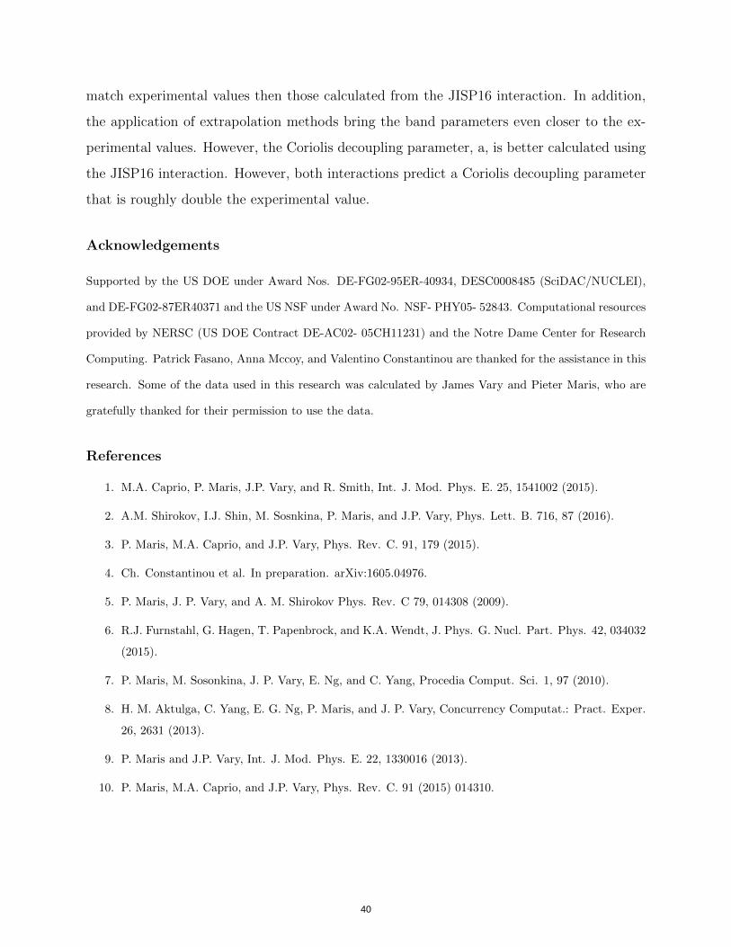
match experimental values then those calculated from the JISP16 interaction. In addition,

the application of extrapolation methods bring the band parameters even closer to the ex-

perimental values. However, the Coriolis decoupling parameter, a, is better calculated using

the JISP16 interaction. However, both interactions predict a Coriolis decoupling parameter

that is roughly double the experimental value.

Acknowledgements

Supported by the US DOE under Award Nos. DE-FG02-95ER-40934, DESC0008485 (SciDAC/NUCLEI),

and DE-FG02-87ER40371 and the US NSF under Award No. NSF- PHY05- 52843. Computational resources

provided by NERSC (US DOE Contract DE-AC02- 05CH11231) and the Notre Dame Center for Research

Computing. Patrick Fasano, Anna Mccoy, and Valentino Constantinou are thanked for the assistance in this

research. Some of the data used in this research was calculated by James Vary and Pieter Maris, who are

gratefully thanked for their permission to use the data.

References

1. M.A. Caprio, P. Maris, J.P. Vary, and R. Smith, Int. J. Mod. Phys. E. 25, 1541002 (2015).

2. A.M. Shirokov, I.J. Shin, M. Sosnkina, P. Maris, and J.P. Vary, Phys. Lett. B. 716, 87 (2016).

3. P. Maris, M.A. Caprio, and J.P. Vary, Phys. Rev. C. 91, 179 (2015).

4. Ch. Constantinou et al. In preparation. arXiv:1605.04976.

5. P. Maris, J. P. Vary, and A. M. Shirokov Phys. Rev. C 79, 014308 (2009).

6. R.J. Furnstahl, G. Hagen, T. Papenbrock, and K.A. Wendt, J. Phys. G. Nucl. Part. Phys. 42, 034032

(2015).

7. P. Maris, M. Sosonkina, J. P. Vary, E. Ng, and C. Yang, Procedia Comput. Sci. 1, 97 (2010).

8. H. M. Aktulga, C. Yang, E. G. Ng, P. Maris, and J. P. Vary, Concurrency Computat.: Pract. Exper.

26, 2631 (2013).

9. P. Maris and J.P. Vary, Int. J. Mod. Phys. E. 22, 1330016 (2013).

10. P. Maris, M.A. Caprio, and J.P. Vary, Phys. Rev. C. 91 (2015) 014310.

40

Developing an Electron Beam Heater for Scanning Tunneling Microscopy

Bridgette Davey

2017 NSF/REU Program

Physics Department, University of Notre Dame

Advisor: Morten Eskildsen

41

Abstract

Scanning Tunneling Microscopy is using a high resolution instrument to image a sample

surface at an atomic level. An electron beam heater (e-beam heater) is an instrument that utilizes

beams of electrons to heat a source target. Electron beam heaters have specific application in

scanning tunneling microscopy which include tip and sample preparation. An ongoing project

exists to engineer an electron beam heater to remove tip contamination, assist in sample

preparation, and allow for the removal of protective oxide layer often used when moving

samples from one institution to another.

Intr oduction

Scanning tunneling microscopy includes the process of taking real-space images on an

atomic scale. Scanning tunneling microscopes make it possible to take the image of a sample as

well as get the electrical properties provided the insulating layers are thin enough to permit

electron tunneling [1]. The physics behind STM involves electron tunneling. In this case

electrons tunnel through a medium (vacuum between the tip and sample being measured) that in

classical mechanics they would otherwise be unable to [2]. With STM microscopes a tip, or very

thin wire, that is conducting is brought very close to a surface to be examined. A bias is then

applied between the sample and the tip. This bias is what allows electrons to tunnel through the

space between the two, hence the term electron tunneling. This stream of electrons tunneling

between the tip and the sample is known as the tunneling current. Tunneling current is a function

of the applied voltage, tip position, and local density of states of the sample [3]. The current

42

between the tip and the sample is measured and converted into an image as the tip scans across

the surface of the sample.

An electronic beam heater is an instrument that uses a stream of electrons to heat a source

object. There are two main types of electron beam heater [4]. One operates purely through

passing a current directly through the sample being heated and the other operates through

thermionic radiation from a filament close to the sample holder. In both cases resistive heating is

utilized. An electron beam heater using a filament has been built in this case due to the

conductive nature of the samples. A large amount of current is required to heat the samples due

to the very low resistance.

Application

There are two common problems in the field of scanning tunneling microscopy that an

electron beam heater addresses. One is sample contamination and another is tip contamination.

Tips are usually made from Tungsten, Gold, or Platinum-Iridium. Inside the lab the tip is

created through an electrochemical etching method. A mixture of potassium hydroxide is used

with a voltage of 4 volts running through it. The tip is coated in a plastic material and submerged

in the solution just beneath the top of the plastic. The solution will then etch away at the metal

until it drops to the bottom of the beaker and a sharp “tip” has formed. The tip is covered by a

thin native oxide layer that needs to be removed in order to maintain stable tunneling conditions

inside the STM [4]. Heating the tip using an electron beam heater removes the oxide layer. Tips

may also become contaminated from transferral from the air into the vacuum chamber. An

43

electron beam heater can remove these contaminants that would otherwise interfere in taking

current measurements.

Another application of an e-beam heater is in the preparation of a sample. Samples may

become contaminated as well through exposure to air or by other means. In order to prevent this

many samples are coated in a protective oxide layer when being transported from one facility to

another. Placing the sample on an electron beam heater and heating it to the appropriate

temperature removes this protective coating.

Design

The current working model of the electron beam heater is shown below.

44

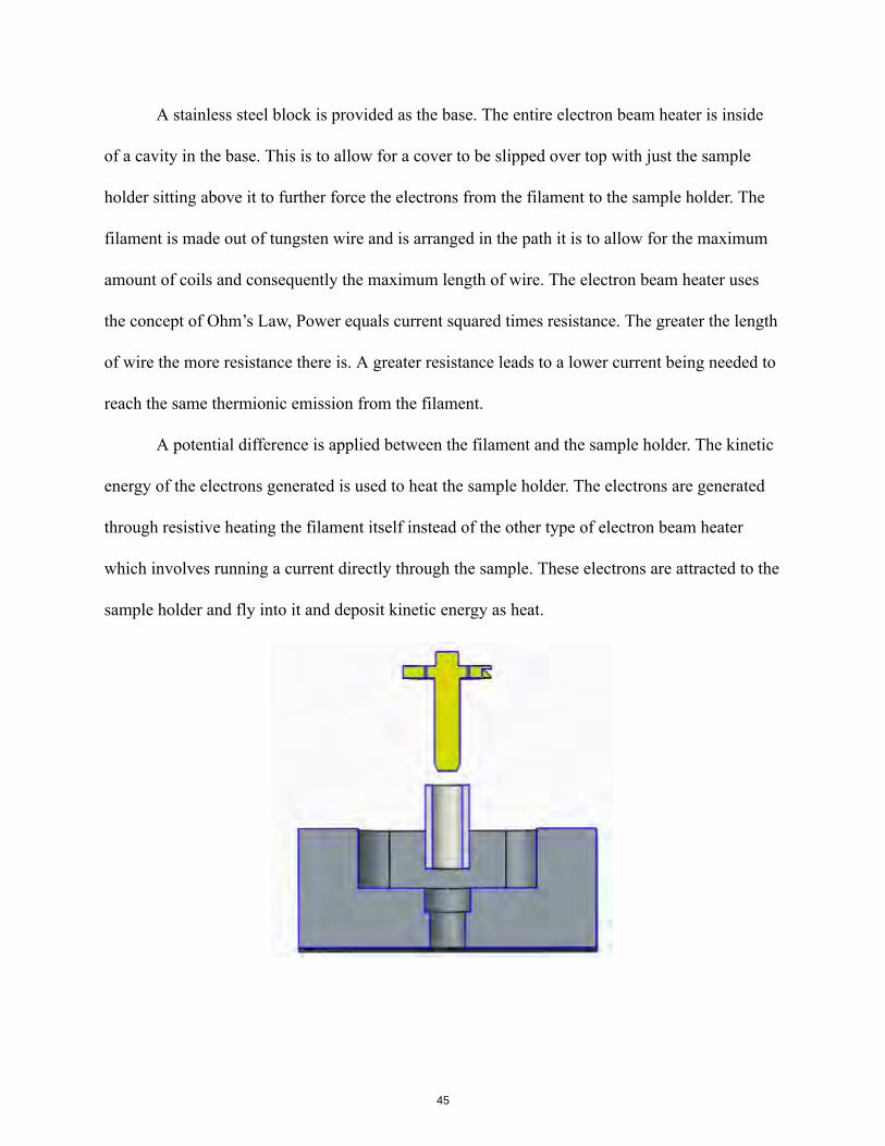
A stainless steel block is provided as the base. The entire electron beam heater is inside

of a cavity in the base. This is to allow for a cover to be slipped over top with just the sample

holder sitting above it to further force the electrons from the filament to the sample holder. The

filament is made out of tungsten wire and is arranged in the path it is to allow for the maximum

amount of coils and consequently the maximum length of wire. The electron beam heater uses

the concept of Ohm’s Law, Power equals current squared times resistance. The greater the length

of wire the more resistance there is. A greater resistance leads to a lower current being needed to

reach the same thermionic emission from the filament.

A potential difference is applied between the filament and the sample holder. The kinetic

energy of the electrons generated is used to heat the sample holder. The electrons are generated

through resistive heating the filament itself instead of the other type of electron beam heater

which involves running a current directly through the sample. These electrons are attracted to the

sample holder and fly into it and deposit kinetic energy as heat.

45

As the previous diagram illustrates, the sample holder is mounted on a ceramic tube to

both prevent the holder from touching the base and prevent the holder from falling through a

hole cut for a connection point for the high voltage line.

Testing

The first step in testing the current electron beam heating design is mounting the instrument

inside of a vacuum chamber as it will have to function under vacuum conditions. The layout of

the system used to test it is shown above. A viewing window exists to the side of the chamber to

provide visual contact. The combination of the vacuum and ion pump can bring pressure inside

the vacuum chamber down to 10^-7 mbar.

After the heater is mounted inside of the vacuum and connected through the ports in the

side to the ground, voltmeter, and high voltage line the vacuum is pumped down to a minimum

46

of 10^-6 mbar. Once pumped down a current is applied to the filament with a voltage of 1000

volts running through it. The filament begins to glow (as we have in fact created a lightbulb, a

tungsten filament in vacuum). The sample holder itself only begins to heat up when high voltage

has been turned on as can be demonstrated in the images below.

Further Steps

Developing an electron beam heater is an ongoing process. Some aspects to take into

consideration in the future are trying to get the current even lower to attain the same heating

capabilities it has now at 1000 volts. One possibility would be in using a different type of wire

with a similar melting point to tungsten. A wire such as stainless steel is relatively useless as it

would melt almost instantly. Another possibility is trying a thinner wire with the same parallel

path and working to get more wire length through a greater number of spirals. Eliminating the

screws and finding a way to hold the filament up with just the tungsten wire would also be ideal

as the screws are giant heatsinks. All in all an electronic beam heater is a useful instrument in

addressing three problems in scanning tunneling microscopy: tip contamination, sample

preparation, and removing protective packaging on samples.

47

Acknowledgements

I wish to thank my advisor Dr. Morten Eskilden and graduate students Allan Leishman and

David Green for working with me this summer. I have learned a great deal this summer that

without their support and seemingly unending patience would have been impossible. I would like

to thank David Green specifically for teaching me how to use Creo Parametric and working

with/giving me the background knowledge to design a helium recovery system. I wish to thank

Allan Leishman specifically for working with/giving me the background knowledge to work on

designing the e-beam heater. Last but certainly not least I would like to thanks Dr. Umesh Garg

for the impossibly wonderful chance to do an REU and research here at Notre Dame, and Lori

Fuson and Nell Collins for program coordination.

Refer ences and Notes

1. Binnig, G., & Rohrer, H. (1983). Scanning Tunneling Microscopy. Surface Science,

126(1-3), 236-244.

2. Binnig, G., & Rohrer, H. (2000). Scanning Tunneling Microscopy. IBM Journal of

Research and Development, 44(1), 279-293.

3. Julian Chen, C. (1993). Introduction to Scanning Tunneling Microscopy. Oxford

University Press. 0-19-507, 150-6.

4. Ding, H. F., et al. (2005).Electron-beam Tip/sample Heating Device for a Scanning

Tunneling Microscopy. Review of Scientific Instruments 76.12, 123703.

5. Behrisch, R. (1981). Sputtering by Particle Bombardment. Berlin, Springer. Vol 1.

48

EFFECTS OF SUMMER CAMP ON PARTICIPANTS’ AFFECTIVE VIEWS OF

SCIENCE

Iliana De La Cruz

2017 NSF/REU Program

Physics Department, University of Notre Dame

ADVISOR: Dr. Micha Kilburn

49

ABSTRACT

There exists a movement to draw more diverse groups of students to science, technology,

engineering, and math (STEM) careers with recent data suggesting students select STEM tracks

as early as high school with influence starting as early as middle school. Yet, limited research

exists on K-12 students and how their affective views of science are influenced by outreach. This

research quantitatively examines the effect of a summer camp on participants’ affective views of

science by age, gender, and career aspirations. Camp participants were offered a survey at the

beginning and end of each week long camp asking them to rate how much they like art, science,

math and engineering, their career aspirations, and which words they associate to science or art

from a predetermined list. Researchers analyzed four years of these programmatic surveys

seeking any relation between words associated to participants’ age, gender, and career

aspirations. This summer, researchers also interviewed camp participants to further understand

their perspectives during the survey and word associating process to evaluate the effectiveness of

the survey itself. Preliminary statistical analysis suggests the camp significantly affects

participants’ career choice with regard to STEM careers. Interview results also highlighted points

of confusion in younger students and different interpretations of words amongst older students,

which can be used to redesign the survey instrument to better asses the effect of the camp

experience.

Keywords: informal education, outreach, affective views, word associations, science summer

camp

50

1 Introduction

Since 2011, the Joint Institute for Nuclear Astrophysics, Center for the Evolution of

Elements (JINA-CEE) has sponsored the “Art 2 Science Summer Camp” hosted at the

University of Notre Dame. Camp intended to introduce students from ages 8-12 to science they

would not usually see in the classroom via a variety of art forms and creative experiments and to

instill a greater sense of hands-on science. Art 2 Science hosts approximately 100-180 student

participants, 25 teenage junior counselors, 12 adult counselors, and 15 adult activity leaders

throughout one week. Students submit applications and are accepted until reaching maximum

occupancy and camps fees are based on a sliding scale according to household lunch fees.1 At

the start of camp participants are asked to complete anonymous surveys with the option to not fill

one out, this action is repeated at the end of the camp as well. The pre-camp survey asks for the

participant’s gender, career aspirations, preferred school subjects, rate on how much they like art,

science, math, and building things on a scale of 1-10, and to circle words that sound like science

or triangle words that sound like art or both. The post survey is identical but also asks

participants to rate activities. Dates of birth, are utilized only for matching pre-post and are

deleted afterwards to maintain anonymity.

Data was collected from pre and post surveys over the 2013-2016 summers and recorded

in an Excel sheet. Using software such as Root and Excel to populate comparative histograms

and statistical analysis we questioned:

1. Do students have a significantly more favorable view of science after camp?

2. What defines a favorable view of science?

3. Does there exist a significant relation between words associated to science and

participants’ age, gender, or career choice?

51

After analyzing data accumulated across the four years, researchers also asked:

4. How are students interpreting the questions and words from the surveys?

a. Is the survey effectively measuring camp goals?

These questions were the forefront of the interviewing process. Under Notre Dame IRB

approval, the 2017 Art 2 Science Camp also had researchers conducting interviews with

participants who had both parental and participant consent. Researchers questioned participants’

understanding of the survey, reasoning behind career choice, explanation for science and math

ratings, and further explanation for their word associations and how the instructions/words were

interpreted. The purpose of conducting interviews was to get more insight for trends seen in

preliminary 2013-2016 data analysis.

2 Methods

Survey responses were coded to categorize responses in a numerical way to then translate

data to plain text files and read into Root code. For example, careers were categorized as STEM

(on account of degree required), sports, artistic, medical/health related, miscellaneous, and

unsure.

(Figure 1) (Figure 2)

Career Chosen: 0=Unsure, 1=STEM, 2=Arts, 3=Sports, 4=Med/Vet, 5=Misc0 1 2 3 4 5 60

20

40

60

80

100

Pre careers chosen

MaleFemale

Carrer Chosen: 0=UUnsure, 1=STEM, 2=Arts, 3=Sports, 4=Med/Vet, 5=Misc0 1 2 3 4 5 60

20

40

60

80

100

Post careers chosen

MaleFemale

52

Bar charts with standard mean error were used to estimate the percentages of participants

associating a specific word to science grouped by age (Figure 3). But standard with human

studies, reporting error bars are only

Figure 3

tentative and cannot take into account all possible factors. Associated word bar charts were

utilized in analyzing data from across the four years to realize trends or queries to further inspect

with statistical analysis. Only words repeated throughout the four years were analyzed for

consistency which narrowed analysis to fifteen words.

Analysis compared data in search of statistical significant change i.e. if camp affected

participants’ survey responses or if specific groups of students had significantly different word

associations. Statistical significance was calculated using a two tailed t-test comparing the pre to

post survey responses. Calculating the significance between participant markers like gender, age,

and career and the words associated in either pre or post surveys was done using a Chi-squared

statistic. P values were calculated using the CHISQ.TEST in Excel comparing gender to words

associated in both pre and post surveys, comparing gender to words but specifically in smaller

age groups, and in comparing gender to words within only STEM majors. In comparing pre

survey data with post survey data p values were calculated using the T.TEST function in Excel.

Both tests were analyzed with the standard significance value of 0.05 in search of a p<0.05.

Age (years)8 8.5 9 9.5 10 10.5 11 11.5 12 12.5 13

Frac

tion

Affir

mat

ive

0

0.2

0.4

0.6

0.8

1

MaleFemale

Science is Hard

53

Interviews were conducted with volunteered participants who submitted both parental

and participant consent on the first day of camp. Interview questions were geared toward

understanding the participants’ perceptions of the survey questions. Analyzing graphs for word

associations brought up questions about participants paradoxically associating antonyms.

Volunteered participants were asked for clarification regarding the words they selected for

science, especially words seeming to contradict each other and words researchers perceived

potentially misunderstood or interpreted differently such as ‘elderly’, ‘reading’, ‘same’, and

‘future’. Participants were also asked regarding the ratings they gave science and math after

noting a discrepancy in the 2016 survey data between participants’ ratings of science and liking

math (Figures 4 and 5). As a last interview question, students were asked to

Figure 4 Figure 5

re-select words they thought a scientist would associate to science. This question was asked to

gain a foundational understanding of how participants abstractly viewed science.

3 Results

Histograms showed gender gaps in word associations and also in pre-post career choices

(Figures 1 and 2). Statistical analysis was used to determine if student characteristic such as age,

gender, or career aspiration affected word associations. Also, interview results provided insight

Age (years)8 8.5 9 9.5 10 10.5 11 11.5 12 12.5 13

Scal

e 1-

10

0

2

4

6

8

10

MaleFemale

Like Science

Age (years)8 8.5 9 9.5 10 10.5 11 11.5 12 12.5 13

Scal

e 1-

10

0

2

4

6

8

10

MaleFemale

Like Math

54

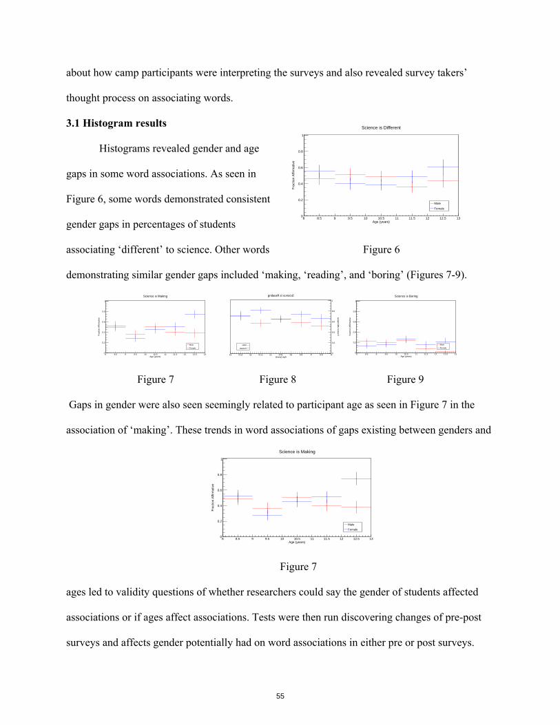
about how camp participants were interpreting the surveys and also revealed survey takers’

thought process on associating words.

3.1 Histogram results

Histograms revealed gender and age

gaps in some word associations. As seen in

Figure 6, some words demonstrated consistent

gender gaps in percentages of students

associating ‘different’ to science. Other words Figure 6

demonstrating similar gender gaps included ‘making, ‘reading’, and ‘boring’ (Figures 7-9).

Figure 7 Figure 8 Figure 9

Gaps in gender were also seen seemingly related to participant age as seen in Figure 7 in the

association of ‘making’. These trends in word associations of gaps existing between genders and

Figure 7

ages led to validity questions of whether researchers could say the gender of students affected

associations or if ages affect associations. Tests were then run discovering changes of pre-post

surveys and affects gender potentially had on word associations in either pre or post surveys.

Age (years)8 8.5 9 9.5 10 10.5 11 11.5 12 12.5 13

Frac

tion

Affir

mat

ive

0

0.2

0.4

0.6

0.8

1

MaleFemale

Science is Making

Age (years)88.599.51010.51111.51212.513

Fraction Affirmative

0

0.2

0.4

0.6

0.8

1

MaleFemale

Science is Reading

Age (years)8 8.5 9 9.5 10 10.5 11 11.5 12 12.5 13

Frac

tion

Affir

mat

ive

0

0.2

0.4

0.6

0.8

1

MaleFemale

Science is Boring

Age (years)8 8.5 9 9.5 10 10.5 11 11.5 12 12.5 13

Frac

tion

Affir

mat

ive

0

0.2

0.4

0.6

0.8

1

MaleFemale

Science is Making

Age (years)8 8.5 9 9.5 10 10.5 11 11.5 12 12.5 13

Frac

tion

Affir

mat

ive

0

0.2

0.4

0.6

0.8

1

MaleFemale

Science is Different

55

3.2 Significant results

Statistical analysis suggests gender affected participants’ association of the word

‘different’ to science and camp affected participants’ associations of ‘fun’ and ‘making’. Using

the CHISQ.TEST function in Excel, researchers found p<0.05 thus leading to rejecting the null

hypothesis, H0, in gender to post-survey associations of ‘different’ suggesting post associations

were affected by the gender of the participant. The T.TEST Excel function comparing post-

surveys to pre-surveys found p values less than .04 for words ‘fun’ and ‘making’ therefore

leading to a rejection of H0 for pre associations of the words are not independent of the post

associations suggesting camp does affect participant associations. In comparing pre to post

associations and gender to pre/post associations researchers discovered significant p values for

only these three words out of the fifteen repeated words. This evidence led to further questions

about potential gender effects to associations within smaller age groups of participants.

Questions about participants’ understanding of words that might explain their differences in

associations were addressed in the interviews conducted during the 2017 Art 2 Science camp.

3.3 Interview results

Interviews further explained participant understandings of individual words and survey

questions. Younger students, aged 8-10, experienced difficulty understanding words used in

2016 and 2017 surveys ‘youth’ and ‘elderly’. Some participants also made associations by

considering inside and outside their classrooms; like when associating ‘hard’ and ‘easy’ students

reflected science problems and ideas as hard but experiments and class projects as easy.

Researchers also found most students consider varying aspects of science in associating ‘new’

and ‘old’ like understanding science has existed long before them and even today scientists are

making discoveries. The youngest group of students, ages 8-9, did express misunderstandings of

56

the questions from the surveys. One example was associating words that rhyme with science

because the words literally sounded like science. Other students expressed thinking all words on

the survey had to be marked in some way even though there were words they did not understand

and disagreed with. Interviews clarified reasons behind students seemingly associating

paradoxical words but results also put the overall surveys into question since student

interpretations of questions did not match with expected interpretations made by researchers

4 Conclusions

Histograms showed gender gaps in Figures 6-9 and also showed interesting changes

between ages of participants and their word associations in describing science. Students appeared

to have significantly changed views for the words ‘fun’ and ‘making’ when comparing pre-post

surveys and gender was significant for the word ‘different’ associated in post-surveys. This leads

to further questions on the relation between characteristics of participants such as age or career

aspirations and their word associations and if any other connections show significant effects.

Interview responses used to interpret student understandings bring validity of the current survey

used into question so preliminary results lead researchers to expect changes to how questions of

associations are phrased and possibly another change of listed words.

57

References

[1] Kilburn, M. "Art 2 Science Summer Camp." Joint Institute for Nuclear Astrophysics, Center

for the Evolution of Elements, 10 Apr. 2017. Web. 22 July 2017.

Appendix

Pre and post surveys:

Birthdate (month, day) _______________________

Are you a: boy girl

How many times have you attended this camp before (0,1,2,3) ___

What career/job do you want when you're older? ______________________________________________

What subjects do you like in school?_______________________________________________

On a scale of 1-10, with 10 being the most:

How much do you like art? 1 2 3 4 5 6 7 8 9 10How much do you like science? 1 2 3 4 5 6 7 8 9 10How much do you like math? 1 2 3 4 5 6 7 8 9 10How much do you like building things? 1 2 3 4 5 6 7 8 9 10

Circle words that sound like science

Put triangles around words that sound like art

Words can have both a circle and a triangle

funhard play

different

doing watching

creative

elderly

new old

makingreadingsame

workeasyboring

youthancientfuture

rules

Birthdate (month, day) _______________________

What career/job do you want when you're older? ______________________________________________

On a scale of 1-10, with 10 being the most:

How much do you like art? 1 2 3 4 5 6 7 8 9 10How much do you like science? 1 2 3 4 5 6 7 8 9 10How much do you like math? 1 2 3 4 5 6 7 8 9 10How much do you like building things? 1 2 3 4 5 6 7 8 9 10How much did you like camp? 1 2 3 4 5 6 7 8 9 10

What will you tell your friends about JINA Art 2 Science Camp?__________________________________________________________________________________________________________________________________________

Circle words that sound like science

Put triangles around words that sound like art

Words can have both a circle and a triangle

funhard play

different

doing watching

creative

elderly

new old

makingreadingsame

workeasyboring

youthancientfuture

rules

58

CALCULATING ELECTRON DRIFT VELOCITY &

COMPLETING COMPONENTS OF ND CUBE

Lauren Delgado

Advisor - Dr. Tan Ahn

2017 NSF/REU Program

Physics Department, University of Notre Dame

59

ABSTRACT

Calculations of drift velocity and ion straggling were obtained for a helium carbon dioxide mixture

inside a time projection chamber (TPC). Because this gas detector could control parameters

like electric field and pressure, these were altered to observe the relationships of those variables

that could improve the quality of the experiment for studying cluster structure in nuclei. This

collection of data would be significant for use in future analysis and comparison to experimental

results. To use this detector, the construction of an electric field cage and feedthrough system

were completed so that a test run could be made to gain preliminary results. These components

will be tested for their efficiency by performing the experiment and examining whether the

measurements produced results found computationally.

INTRODUCTION

Stars are formed from dust clouds containing hydrogen (H) and helium (He) collapsing into one

another. Stars join the main sequence for about 90% of their lives, where they evolve depending

on their mass. To focus on high mass stars, these stars (> 8 M¯) reach high enough temperatures

to burn elements beyond helium like carbon, oxygen, and so on till iron. This type of reaction

describes nucleosynthesis, which is the creation of new atomic nuclei. Atomic nuclei are a

central focus within this project. The production of lighter nuclei and studying their interactions

with light ions offers information. By analyzing the properties and behavior of nuclei, this allows

us to ”attain a deeper and more precise understanding of the many nuclear processes operating

in astrophysical environment” (1). The goal is to understand what the structure of nuclei, by

studying lighter nuclei, suggests about the formation of heavy metals beyond iron in some

astrophysical scenarios.

60

GAS FILLED COUNTERS

Because the nucleus cannot be directly observed from its size (1 Å 1.75 ·10−15), information

about the nucleus can be obtained through special equipment. This type of equipment has the

capability of detecting radiation and also producing nuclei by accelerating charged particles.

Within the scope of this experiment, the usage of gas proportional counters is crucial in order

to measure particles of ionizing radiation. A gas proportional detector will bombard electrons

with gas molecules frequent enough to create an avalanche of them to drift to the anode that

will create a pulse. Usually in these detectors they are filled with noble gases since they are not

electronegative. This device in this experiment will operate similarly.

(a) Example of a Gas Filled Counter (b) Townsend Avalanche

Figure 1: Looking at Gas Filled Counters (Credit to Oak Ridge Associated Universities Webpage onProportional Counters)

61

ND CUBE FUNCTION

The ND Cube is a prototype TPC that is being used for this experiment. The cube stands out from

normal gas detectors because it "uses a gas volume as [both] the target and tracking medium"

(2). The dual use of the gas provides extreme precision for angle and energy measurements from

charged-particle decays and higher areal densities that contain information about properties of

those particles in the reaction. Thus, this device is advantageous for learning more about nuclear

structure and looking at fusion.

METHOD OF USING ND CUBE

First, the ND Cube is filled with a gaseous mixture from a gas handling system it is connected

to. Then heavy ion beams are sent into it where it interacts with the gas present inside. A large

electric field is applied to the cage located inside. The heavy-ion beam ionizes the gas molecules

as it collides with them. Free electrons begin to drift in the detector. Electrons drift to the bottom

of the cube, towards a higher potential, at a constant velocity. At the bottom of the detector there

is an amplification device (Micromegas) that collects these electrons and produces in a signal

from them and redirects this out to the front-end electronics. Within this specific experiment,

drift velocity and straggling of ions are the focus because these parameters will affect the position

of the identified radiation.

ELECTRON DRIFT VELOCITY

Calculations of drift velocity were made as a function of electric field and pressure for a helium

carbon dioxide mixture. The results for velocities were obtained using a bash script that ran two

programs named Magboltz (created by CERN) and Decode.

62

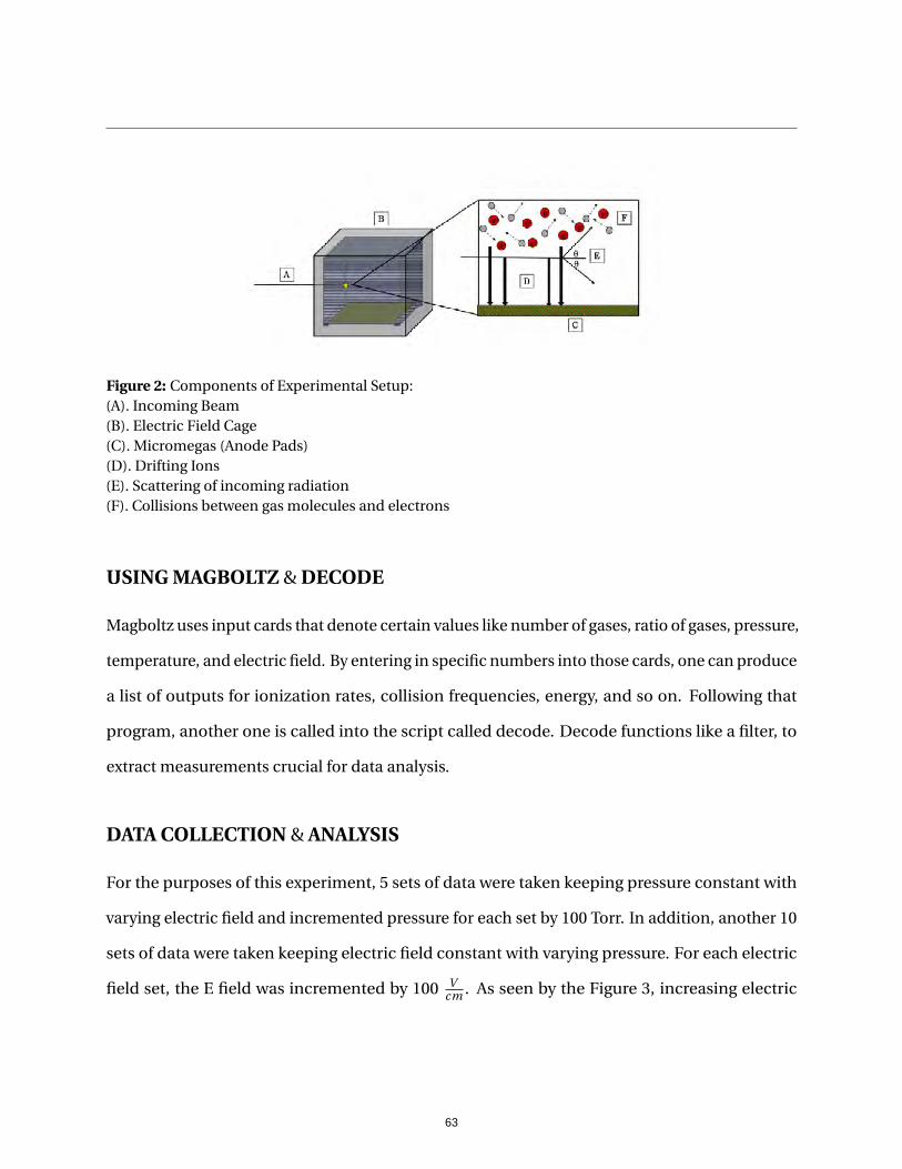
Figure 2: Components of Experimental Setup:(A). Incoming Beam(B). Electric Field Cage(C). Micromegas (Anode Pads)(D). Drifting Ions(E). Scattering of incoming radiation(F). Collisions between gas molecules and electrons

USING MAGBOLTZ & DECODE

Magboltz uses input cards that denote certain values like number of gases, ratio of gases, pressure,

temperature, and electric field. By entering in specific numbers into those cards, one can produce

a list of outputs for ionization rates, collision frequencies, energy, and so on. Following that

program, another one is called into the script called decode. Decode functions like a filter, to

extract measurements crucial for data analysis.

DATA COLLECTION & ANALYSIS

For the purposes of this experiment, 5 sets of data were taken keeping pressure constant with

varying electric field and incremented pressure for each set by 100 Torr. In addition, another 10

sets of data were taken keeping electric field constant with varying pressure. For each electric

field set, the E field was incremented by 100 Vcm . As seen by the Figure 3, increasing electric

63

(a) Varying Pressure in He:CO2 (b) Varying Electric Field in He:CO2

Figure 3: Effects of Pressure and Electric Field on Drift Velocity

field, also increases the drift velocity. However, another feature of the data shows that pressure

increased slows the drift velocity. This inverse relationship illustrates that keeping pressure low

would achieve higher drift velocities. Hypothetically, during performing the actual experiment,

pressure would be fixed so the electric field strength needs to be varied to optimize the velocity.

ION STRAGGLING

Information other than drift velocity, like the diffusion coefficient, was further analyzed. The

diffusion coefficient, di f fco , offered information about the straggling of the ions, σ, when

moving through the cube. Ions typically straggle when they enter another medium, meaning

they deviate from their initial trajectory. Straggling is relevant because it should be minimized

for this type of experiment. Both the longitudinal and transverse straggling were computed using

diffusion coefficient, following this formula

σ(µm) = di f fco ·√

leng th (1)

64

DATA COLLECTION & ANALYSIS

Similar to the data acquired for drift velocity, 5 sets of data were taken keeping pressure constant

with varying electric field and incremented pressure for each set by 100 Torr. Then another 10 sets

of data were taken keeping electric field constant with varying pressure. For each electric field set,

the E field was incremented by 100 Vcm . However, this produced twice the amount data because

there were two types of straggling to examine: longitudinal (along the beam direction) and

transverse (perpendicular to the beam direction). Figure 4 shows how changing pressure affects

(a) Changing Pressure on Longitudinal Straggling (b) Changing Pressure on Transverse Straggling

(c) Changing E-Field on Longitudinal Straggling (d) Changing E-Field on Transverse Straggling

Figure 4: Effects of pressure and electric field on ion straggling in both the longitudinal and transversedirections. Length for ion travel is 10 cm in this run of data.

65

longitudinal and transverse straggling of ions when electric field is kept constant. Evidently,

increasing pressure, lowers the amount of straggling of ions in either direction. Therefore, it

would be optimal to secure the detector at a high enough pressure to reduce straggling. Electric

field strength had no uniform effect on transverse and longitudinal straggling. Overall, frequently

there were higher values for transverse straggling as opposed to longitudinal straggling in all

sets of data. For each trial, 10 and 20 cm sample lengths were used to observe whether the

(a) Changing Pressure on Longitudinal Straggling (b) Changing Pressure on Transverse Straggling

(c) Changing E-Field on Transverse Straggling (d) Changing E-Field on Longitudinal Straggling

Figure 5: Effects of increased length for ion to travel on straggling in both the longitudinal and transversedirections. Length for ion travel is 20 cm in this run of data.

distance traveled by the ions affected the amount of ion straggling that would take place. The

prediction was that the more distance the ions would have to travel, the more straggling would

66

take place. This hypothesis was reflected accurately in the results collected. The highest value

for longitudinal straggling in Figure 4 (a) for a 10 cm path reached 2500 µm, whereas the highest

value for the 20 cm path was 3500 µm in Figure 5 (a). This trend was established throughout the

other data too.

RESISTOR CHAIN

Inside the ND Cube, previous students had built an electric field cage with 21 metal conducting

rings to produce a uniform electric field. Recently the resistor chain was completed as part of

this project. This chain is crucial to the experiments because it provides the uniform electric

field needed. This field is created by the even spacing of rings on the cage. Every ring will divide

the voltage applied by the number of rings present. Therefore, the combination of the number of

rings and even spacing between them maintains uniform field strength. The resistor chain was

finished through soldering.

SOLDERING PROCESS

Soldering is a technique used to create permanent connections between electronic components.

Each resistor within the chain had 20 megaohm resistance. First, two resistors were connected

by placing them inside the same lug terminal and then those connections were crimped into

place to stay secure. To successfully solder each connection properly without damaging the

resistor itself, two clamps acting as heat sinks had to be placed where the ring and lug terminal

met and where the wire of the resistor extended. Then, the electric field cage was turned on its

side. With a soldering iron gun, the lug terminal was heated with metal wire, which solidified the

connection. This was repeated multiple times until the chain was complete. After this was done,

67

(a) Resistor Chain Outlined Design (b) Upclose Image of Resistor Chain

Figure 6: Resistor Chain Connections

a digital multimeter was used on every two resistor connections to check their resistance and

make sure they were successfully connected by the soldering process.

FEEDTHROUGH SYSTEM

For the final leg of the project, the ND Cube required feedthroughs to make sure the electronics

could receive the information from the experiment. For that reason, the final feedthrough design

included a high voltage feedthrough entering from the top of the detector that connected to the

cathode plate at the top of the electric field cage. Along with that, on the right side of the cube,

five holes were made on an end cape for 3 BNC (coaxial) connectors and 2 SHV (high voltage)

connectors. The design’s practicality is that the single ended SHV connector from the top of

68

the cube can conveniently drop a wire down onto the cathode plate. The wire would not bend

and could attach easily. The bottom 2 SHV connections are significant because they are located

closely to the Micromegas, but can also reach the second to last ring where the field cage is

grounded. Because of that placement, signals from the cube can reach out from the electronics

into a computer located beside it.

(a) Feedthrough Design (b) Upclose Image of Completed Feedthrough

Figure 7: Feedthrough System

REFERENCES

1. Claus E. Rolfs and William Rodney, Cauldrons in the Cosmos: Nuclear Astrophysics by Claus

,(XVI)

2. University of Notre Dame: ISNAP Experimental Setups Page, "Prototype Active-Target

Time-Projection-Chamber"

69

70

!

PIXE%and%XRF%Analysis%of%Roman%Denarii!!!!!!!

Cecilia!Fasano,!M.!Raddell,!K.!Manukyan,!E.!Stech!,M.!Wiescher!

Notre%Dame%Department%of%Physics!|!July%2017%

71

Abstract: A set of Roman Denarii from the republican to the imperial period (140BC-240AD) has been studied using X-ray fluorescent (XRF) scanning and proton induced x-ray emission (PIXE) techniques. XRF and PIXE are commonly used in the study of cultural heritage objects because they are nondestructive. The combination of these two methods is also unique because of the ability to penetrate the sample with a broader spectrum of depths and energies than either could achieve on its own. The coins are from a large span of Roman history and their analysis serves to follow the economic and political change of the era using the relative silver and copper contents in each sample. In addition to analyzing the samples, the study sought to compare these two common analysis techniques and to explore the use of a standard to examine any shortcomings in either of the methods. Data sets were compared and then adjusted to a calibration curve which was created from the analysis of a number of standard solutions. The concentrations of the standard solutions were confirmed using inductively coupled plasma spectroscopy. Through this we were able to assemble results which will progress the basis of understanding of PIXE and XRF techniques as well as increase the wealth of knowledge of Ancient Roman currency. Introduction: Through the use of micro-XRF and PIXE, data of the relative elemental compositions of a number of Roman Denarii from 140BC-240AD were collected and analyzed. The data were then analyzed to give specific quantifications, by weight, of the bulk elements and trace elements of the coins. From these data we were able to create a visual representation of the changing silver and copper contents throughout the entire timeline of the samples. The Silver Denarius was introduced in 201 BC after the Punic wars as the new silver standard coinage of the Roman republic. The Denarius was minted from virtually pure metal (99-99.5% fine). With an initial standard of 72 Denarii (4.5g) minted from one pound of silver (322.5g) it proved to be stable enough to help finance the expansion of the empire (200-91BC) and the challenges of the civil wars of the first century (90-31BC). During the civil wars devaluation occurred by gradually reducing the weight so that 84 Denarii of 3.8g each were minted from one pound of silver. This value was established as a new standard of the Augustan currency reform. The Denarius continued to be used as standard coinage during the first 200 years of the imperial period but was devalued several times by reduction of the silver content. Experimental Arrangements: For the PIXE analysis of the coins, the experiments were performed at the 10 MV FN Pelletron Tandem accelerator at the Nuclear Science Laboratory (NSL) of the University of Notre Dame. Proton beams with less than 5 nA intensities were used after penetrating through a 6 µm thick

72

aluminized mylar window to probe the coins, which were positioned at a distance of 2.6 cm from the exit window. The x-rays were analyzed using a Ortec SLP Series Lithium-Drifted Silicon detector with a 0.5 mm Be window and an active diameter of 10 mm positioned at a 40 degree backward angle with respect to the beam direction. For the XRF analysis of the coins, the experiments were performed in part on the Bruker Handheld XRF at the NSL at the University of Notre Dame and in part on the ORBIS XRF machine at the Center for Environmental Science & Technology (CEST) lab at the University of Notre Dame. The Bruker Handheld device contains a rubidium source and was used exclusively for single point analysis. Each coin was scanned three times for a duration of 180 seconds. The number of runs and the time duration were instrumental in ensuring a consistent result. The beam was approximately 1mm in size and the detector was positioned at a 45-degree angle. An aluminum filter was used to block out as much background as possible which allowed for a more accurate quantification.

The ORBIS XRF was used primarily for large scale mapping and a few single point analyses. It was run at a voltage of 40 kV and a current of 400 uA and was run each time with a 25 um Aluminum filter as to stay consistent with the handheld device. To do large scale mapping, the machine triggers the x-ray beam many hundreds of times over the entire specified area. A 30 micrometer beam was used and the spacing between each data point was between 70 and 95 um. This allowed for a large number of points to be taken and for a more accurate image to be created. The images, as part of figures 1 and 2 below, are color coded for each element. For single point analyses, a 1mm beam spot was used.

Table 1 lists the Denarii which were used in this study by their period of minting. The obverse and reverse sides of coins are shown in figures 1 and 2.

Lucretius Trio 136 BC Marcus Aurelius 149 AD Publius Clodius 42 BC Commodus 189 AD

Markus Antonius 31 BC Septimus Severus 197 AD Tiberius Septimus Severus 199 AD

Nero 65 AD Geta (as Caesar) 200 AD Vespasian 74 AD Caracalla 213 AD

Trajan 107 AD Elagabalus 220 AD Trajan 115 AD Severus Alexander 224 AD

Antoninus Pius 140-144 AD Maximinus I 235 AD Marcus Aurelius 145-146 AD Gordian III

The coins included three Denarii from the republican period. One was minted by the Gnaeus Lucretius Trio in 136 BC during the consulate of Sextus Atilius Serranus and Lucius Furius Philus. The second one was minted in 42 BC by Publius Clodius at the beginning of the second triumvirate

73

of Octavianus, Marcus Aemilius Lepidus and Marcus Antonius. The third Denarius was minted in 31 BC after the end of the second triumvirate, a so-called legionary Denarius by Marcus Antonius to pay for his legions in his struggle with Octavian for supremacy.

The coins minted during the first century of the Roman Empire and analyzed in this study include a Denarius minted in 65 AD towards the end of the reign of Nero (54 AD-68 AD), after he had reorganized the Roman mint to finance the rebuilding of Rome after the great fire in 64 AD; a Denarius struck in 74 AD during the last year of the reign of Vespasian (69AD-74AD); two Denarii struck in 107AD and 115 AD during the reign of Trajan (98AD-117AD) honoring his conquests of Dacia and Arabia.

Several of the Denarii included in the study came from the period of the reign of Antoninus Pius (138-161 AD), which characterized a very prosperous and peaceful time of the Roman Empire. One Denarius was minted during the early period 140-144 AD of his reign. Two coins from the same period were minted in 145AD and 149 AD by Markus Aurelius, who served as Caesar with Antoninus Pius before becoming himself emperor (161AD-180AD). The last Denarius from this period of the adoptive emperors was minted in 189 AD under Commodus (180-192 AD), who was the natural son of Marcus Aurelius.

Of particular interest are the coins minted during the period of the Severan emperors, which mostly ruled through military force. The investments in military salaries and the costs for the numerous military campaigns led to gradual debasement of the Denarius. This was investigated by the analysis of two coins minted 197 AD and 199 AD showing the image of Septimus Severus (193-211). During the period of the Severi emperors the silver currency underwent significant fluctuations as outlined before. This should be reflected in the silver content of the coins minted in 197 AD during the short co-reign of Geta (197-211), and in 213 AD during the reign of his brother Caracalla (198-217 AD). A sample of each was studied for this analysis. Also analyzed were Denarii minted during the final years of the Severan period, this included the analysis of Denarii minted under Elagabalus (218-222 AD), Severus Alexander (222-235 AD), and Maximius I (235-238 AD) that are expected to show considerable fluctuations as a consequence of debasement and stabilization policies followed by these emperors. During the reign of Maximius the Denarius was so devalued that his eventual successor Gordian III decided to replace the coin by the Antonianus, which was based on a lower silver content of 70% with respect to the Denarius. For comparison PIXE analysis was also performed at an Antonianus struck in 239-240 AD during the reign of Gordian III (238-244 AD).

PIXE measurements were performed with beam energies of 3.0 MeV for several spots at the obverse and reverse side of each coin for investigating the surface composition of the coins. Some spots were repeatedly measured to check the consistency of the experimental conditions. The results indicate that in most cases the silver-copper composition was consistent for both sides and agreed within less than 2% standard deviation. Only in cases of pronounced surface structure differences in X-ray intensity from the obverse and reverse sides were observed which

74

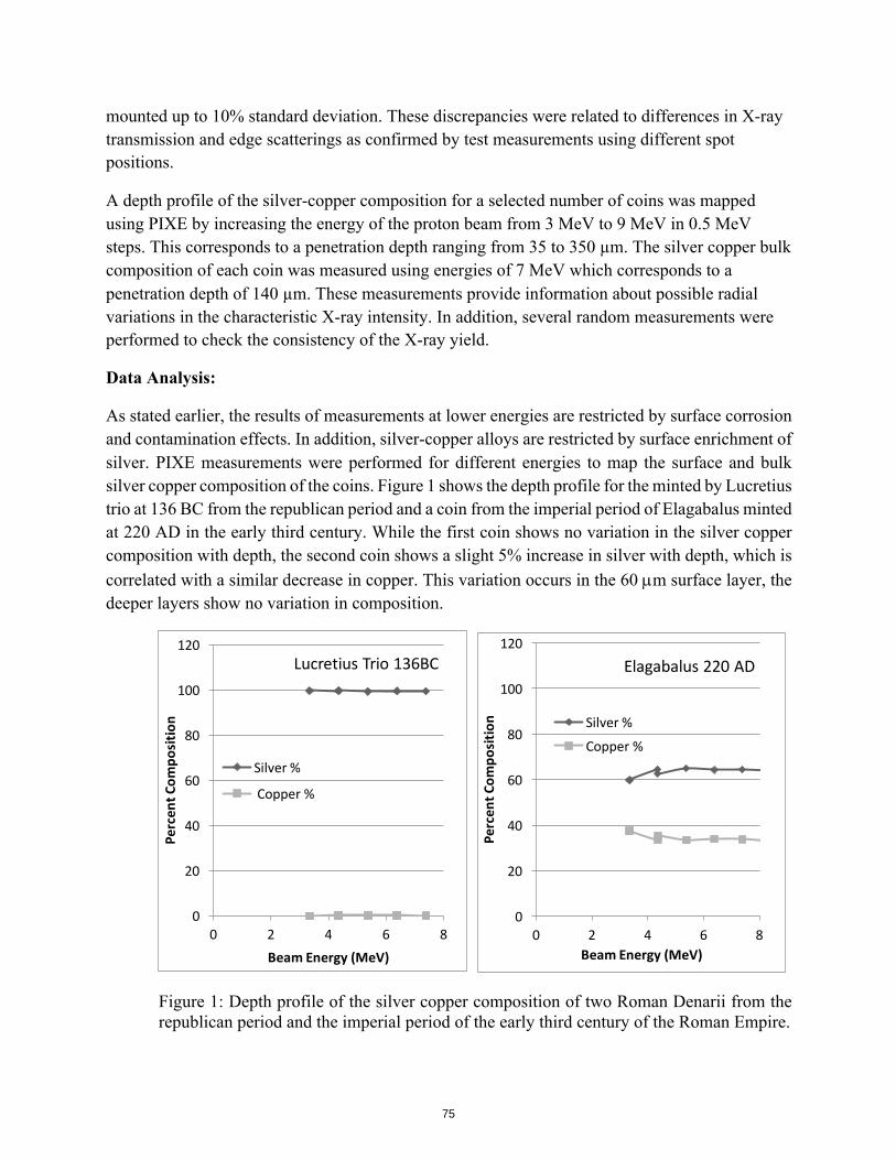
mounted up to 10% standard deviation. These discrepancies were related to differences in X-ray transmission and edge scatterings as confirmed by test measurements using different spot positions.

A depth profile of the silver-copper composition for a selected number of coins was mapped using PIXE by increasing the energy of the proton beam from 3 MeV to 9 MeV in 0.5 MeV steps. This corresponds to a penetration depth ranging from 35 to 350 µm. The silver copper bulk composition of each coin was measured using energies of 7 MeV which corresponds to a penetration depth of 140 µm. These measurements provide information about possible radial variations in the characteristic X-ray intensity. In addition, several random measurements were performed to check the consistency of the X-ray yield.

Data Analysis:

As stated earlier, the results of measurements at lower energies are restricted by surface corrosion and contamination effects. In addition, silver-copper alloys are restricted by surface enrichment of silver. PIXE measurements were performed for different energies to map the surface and bulk silver copper composition of the coins. Figure 1 shows the depth profile for the minted by Lucretius trio at 136 BC from the republican period and a coin from the imperial period of Elagabalus minted at 220 AD in the early third century. While the first coin shows no variation in the silver copper composition with depth, the second coin shows a slight 5% increase in silver with depth, which is correlated with a similar decrease in copper. This variation occurs in the 60 µm surface layer, the deeper layers show no variation in composition.

Figure 1: Depth profile of the silver copper composition of two Roman Denarii from the republican period and the imperial period of the early third century of the Roman Empire.

0

20

40

60

80

100

120

0 2 4 6 8

Percen

t'Com

position

Beam'Energy'(MeV)

Lucretius!Trio!136BC

Silver!%

Copper!%

0

20

40

60

80

100

120

0 2 4 6 8

Percen

t'Com

position

Beam'Energy'(MeV)

Elagabalus!220!AD

Silver!%Copper!%

75

The results indicate that the bulk composition can be measured with proton beam energies for 6 MeV and more. To minimize absorption effects of the low energy X-rays; a beam energy of 7 MeV was chosen for studying the bulk composition of the coins at an average depth level of 140 µm.

To monitor the surface homogeneity of the coin composition a number of PIXE measurements were performed across the surface of each coin. The reverse side showed a more homogeneous pattern with variations between 5% standard deviation. The variation of the characteristic X-ray intensity was more pronounced when scanning the obverse site because of its more pronounced surface structure. The most pronounced variations of sometimes more than 20% deviation from the mean value were observed in the coins from the third century. These probably reflect inhomogeneities in the silver-copper alloy composition as a consequence of re-using coins from earlier rulers as it was frequently the case in the period of unrest in the early third century.

Figure 2: Cross sectional PIXE measurements of the Copper-Silver composition of four Roman Denarii from the first, second, and third century of the Roman Empire. The first two coins represent a homogeneous distribution in the composition within a 2% standard deviation, which reflects the economic and fiscal stability of the Empire after the monetary reform of Nero in 65 AD. The two coins from the early third century show dramatic variations with the silver content being significantly reduced in the central region of the coin. A similar pattern was observed for the coins minted during the reign of Caracalla and Elagabalus. This reflects the overall decline in the quality of the minting process due to

0

20

40

60

80

100

0 5 10 15

Percen

t'Com

position

Run'Number

Nero''65'AD

CopperSilver

0

20

40

60

80

100

0 5 10 15

Percen

t'Com

position

Run'Number

Marcus'Aurelius'145'AD

CopperSilver

0

20

40

60

80

100

0 5 10 15

Percen

t'Com

position

Run'Number

Septimius'Severus'197'AD

CopperSilver

0

20

40

60

80

100

0 5 10 15

Percen

t'Com

position'

Run'Number

Maximius'I''235'AD

SilverCopper

76

limitation to access to silver mines by external war and due to in-mixing of coins from earlier periods.

For single point analysis of the coins using XRF, we were not able to counter the effects of surface corrosion and silver surface enrichment by changing the energy of the beam as was done with the PIXE analysis. The way these issues were combatted with the XRF was by running the beam many different times on multiple locations on the coin. Even with these methods, though, we believe that the deviation between the results of our methods can be mostly attributed to silver surface enrichment and corrosion. As we found through large scale mapping, many of the coins have incredibly inconsistent surface compositions and an inability to penetrate beyond those surface blemishes leads to an inconsistency in the results of different methods and even the results on the same coin using the same method. The x-ray beam used in both the Bruker handheld device and the ORBIS large device was 1mm which only penetrated the coin to a depth of around 200 micrometers. At its deepest, silver surface enrichment can go as far as 500 micrometers into the surface of the coin. Based on these data, the average silver-copper composition has been determined for each of the studied coins and is recorded in Table 2. The references for the republican coinage (Cr) and imperial coinage (RIC) shown in the table relate to the traditional notation for identification of a particular coin as defined in the numismatic literature i, ii.

Coin Notation year Avg %Cu PIXE

Avg %Ag PIXE

Avg % Cu ORBIS

Avg %Ag ORBIS

Lucretius CR 237 136 BC 0.18 99.63 1.91 97.35!Publius Claudius CR 494 42 BC 1.95 97.34 1.83 96.79!Marcus Antonius CR 544 31 BC 5.73 92.69 4.01 94.11!

Tiberius ~ ~ 0.22 98.64!Nero RIC 67 65 AD 3.97 95.90 12.72 86.44!

Vespasian RIC 75 70 AD 9.61 89.38 2.52 96.77!

Trajan RIC 128 107 AD 4.02 94.73 3.99 94.12!Trajan RIC 142 115 AD 7.80 91.23 12.1 87.06!

Antonius Pius RIC 63 140 AD 7.03 92.42 2.44 96.69!Marcus Aurelius RIC 429 145 AD 4.01 95.94 2.51 96.77!Marcus Aurelius RIC 448 149 AD 4.86 95.12 2.03 96.90!

Commodus RIC 192 180 AD 13.59 86.42 2.69 96.56!Septimus Severus RIC 107 193 AD 33.98 66.02 7.24 91.96!Septimus Severus RIC 136 197 AD 36.85 63.16 13.46 85.70!

Geta RIC 18 198 Ad 45.80 53.33 5.97 93.24!Caracalla RIC 224 213 AD 14.59 85.40 3.94 95.28!

Elagabalus RIC 295 220 AD 34.97 63.64 3.93 95.31!Severus Alexander RIC 44 224 AD 4.70 95.26 2.36 96.85!

Maximus I RIC 7 236 AD 25.15 74.85 18.85 79.84! Gordian III RIC 70 240 AD 24.25 74.91 6.10 93.11!

77

For the Bruker XRF device, the data was quantified by looking at the relative numbers of counts for each element and plotted for both silver and copper in chronological order as can be seen below.

Figure 3, the relative counts of silver and copper in each coin as recorded by the handheld device. The bottom axis is the coin number and it is plotted against the number of counts

recorded.

Those relative counts, for silver, were plotted with the weight percent compositions of silver from both the ORBIS and PIXE data sets to create a graph of the silver content of the coins across the total timeline. The left axis is number of counts as measured by the Bruker XRF. The right axis is the percent silver by weight. Each coin was assigned a number in chronological order and are shown on the x axis progressing as a function of time.

0

2000000

4000000

6000000

8000000

10000000

12000000

0 5 10 15 20 25

Silver

01000000200000030000004000000500000060000007000000

0 5 10 15 20 25

Copper

78

Figure 4, the Silver composition of each coin for each method where the bottom axis is the coin number, the left axis is number of counts, and the right axis is percent weight.

As can be seen in the graph, though there are a few inconsistencies, the general trend and shape of the data points is the same across all of the analysis methods. These trends lead us to believe that, within error bars, our data give an accurate representation of the change in elemental composition across the entire timeline of our sample set.

Conclusions: The figure clearly demonstrates the stability of the Roman silver coinage during the period of the Republic after the introduction of the Denarius despite the economic difficulties during the civil wars that led to the fall of the republic and the installation of the imperial system. The figure clearly demonstrates the two decisions for the reformation of the mint by Octavianus Augustus in 25 BC and the debasement by Nero in 65 AD. The silver-copper composition of the Denarius remained rather constant during the subsequent century, smaller fluctuations have been observed which relate to the debasements by Trajan and Marcus Aurelius.

The rapid decline in the silver content of the Denarius at the end of the second and first 40 years of the third century is clearly visible in the data recorded in Table 2 and shown in Figure 3. These drastic devaluation policies were primarily established under Septimus Severus and Geta driven by the costs for maintaining the army and for wars of expansion against the Germanic

0

20

40

60

80

100

120

0

2000000

4000000

6000000

8000000

10000000

12000000

0 5 10 15 20 25

PIXE,!ORBIS!and!Bruker!Silver!Compositions

Bruker Wt%!ORBIS PIXE

79

tribes and the Parthian empire. The attempts of Severus Alexander for stabilizing the monetary stability is reflected in the increased silver content of the Denarius minted at that time. Also reflected in figure 6 is the drastic decline of the Denarius driven by the military expenditures of emperor Maximius I.

From this study, the following conclusions can be drawn. This data allows us to provide evidence for the historical literature and standards of the ancient Roman republic and empire. The silver content over the timeline of the coins matches quite well with the historical context of the era. The use of both PIXE and XRF also allows us to have confidence in the accuracy and precision of our results within our knowledge of the error in the equipment and the inconsistencies in the surface of ancient coins. Future work done in this area will help to more precisely tune and understand both the instruments used in cultural heritage investigation and the numismatics of Roman history.

(These are the sources from the original PIXE paper) i K. W. Harl, Coinage in the Roman Economy, 300 BC to AD 700, John Hopkins University Press, Baltimore & London 1996 i A. Dacca, P. Prati, A. Zucchiatti, F. Luccarelli, P.A. Mando, P .Gemme, R. Parodi, R. Pera, Nucl. Instr. Meth. B161 (2000) 743 i R. Klockenkämper, H. Bubert, K. Hasler, Archaeometry 41 (1999) 311. i V. Kantarelou, F.J. Ager, D. Eugenidou, F. Chaves, A. Andreou, E. Kontou, N. Katsikosta, M.A. Respaldiza, P. Serafin, D. Sokaras, C. Zarkadas, K. Polikreti, A.G. Karydas, Spectrochim. Act. B 66 (2011) 681 !i L. Beck, S. Bosonnet, S. Réveillon, D. Eliot, E. Pilon, Nucl. Instr. Meth. B 226 (2004) 153 !i D. R. Walker, The Metrology of the Roma Silver Coinage: Parts I-III; Brit. Archaeol. Rep. Suppl. 5, 22, 40 (1976-1978) i!A. Denker, K. H. Maier, Nucl. Instr. Meth. B 161-163 (2000) 704-708 i GUPIX reference !i M. H. Crawford, Roman Republican Coinage, 2 Volumes, Cambridge University Press, Cambridge, UK 1974

i Roman Imperial Coinage, Vol. 1-9, eds. C.H.V. Sutherland, R.A.G. Carson, Spink & Son Ltd, London, UK !

!!!!!!!!!!!!!!!!!!!!!!!!!!!!!!!!!!!!!!!!!!!!!!!!!!!!!!!!!!!!!

80

Experimental Determination of the Angular Acceptance of the STrong Gradient Electromagnetic Online Recoil Separator for Capture Gamma

Ray Experiment (St. George) and Observation of Quadrupole Field Reproducibility

Will Feltman

2017 NSF/REU Program

Physics Department, University of Notre Dame

Advisor: Dr. Manoel Couder

Graduate Students: Luis Morales, Chris Seymour, Gwen Gilardy, and Shane Moylan

81

Abstract:

The STrong Gradient Electromagnetic Online Recoil separator for capture Gamma ray

Experiment (St. George) is in the process of determining its experimental limits. Currently the

focus is on determining the angular acceptance of particles entering the St. George beam line.

The demonstration of the current experimental angular acceptance is discussed in addition to the

necessary procedure to ensure that St. George’s quadrupoles generate consistent magnetic fields.

1. Introduction:

For the past centuries scientists have spent a considerable amount of time observing and

studying various types of stars. Thanks to advances in modern science, they have managed to

obtain a good understanding of how stars operate, such as what fuels their fiery existence, how

they produce many chemical elements, and how they die. However, they don’t currently have a

complete understanding of all the various nuclear reactions that occur, which has led to the

creation of new techniques to study stars and various stellar reactions.

Since it is currently impossible to create the conditions of a star in a laboratory, physicists

had to think outside of the box to create a procedure to study the rare reactions that occur in and

around stars. Frequently, nuclear reactions are studied by detecting the gamma rays released

when the reaction occurs. However, with low energy nuclear reactions the gamma production

levels can be so low that it is impossible to separate them from the overall background gamma

radiation, making it necessary for other methods to be created. Inverse kinematics is one such

method in which a heavy ion beam strikes a lighter target. For the reactions which St. George

was designed to study, the sum of nucleons (A) in the beam is greater than four, and the target is

often hydrogen or helium. The STrong Gradient Electromagnetic Online Recoil Separator for

capture Gamma ray Experiment (St. George), located in the Nuclear Science Laboratory at the

82

University of Notre Dame, Notre Dame Indiana was designed and constructed to study nuclear

reactions through the implantation of inverse kinematics.

The construction of St. George, was completed in 2010, and since then has been

preparing to study rare (α,γ) reactions. St. George is composed of eleven quadrupole magnets

(Qn), six dipole magnets (Bn), and a Wien Filter (WF), each of which serve a different purpose,

in addition a series of detectors and viewing quarts have been installed to gather more

information about the ion beam traveling through St. George. The dipole magnets are used to

steer the reacted components though the St. George’s beam line to detectors located at the end.

The quadrupole magnets produce consistent magnetic fields, designed to focus in one spatial

direction while defocusing in another. Magnets Q1, Q4, Q7, Q8, and Q11 focus in the Y

direction while defocusing in the X and magnets Q2, Q3, Q5, Q6, Q9, and Q10 do the opposite.

The Wien Filter, often called a Velocity filter, sorts particles based on their velocities, by

employing both a magnetic and electric field only particles with velocities equal to the electric

field divided by the magnetic field, are allowed to pass through uninhibited. The other particles

that manage to enter the Wien Filter are pushed to the sides and discarded, this allows for only

the particles of interest to be transmitted. A series of three quadrupoles called the triplet is

located shortly before the HIPPO Gas target. This is used to help prepare the beam to enter St.

George.

The beam provided for St. George comes from the 5 MV Stable Ion Accelerator for

Nuclear Physics (5U) which was installed in 2012 and first ran in 2015. Since St. George has

been able to receive beam, its experimental limits have been studied. Previously, the

experimental limits of the energy acceptance of St. George was been determined. This was

demonstrated by individual experiments in which eight different beams were delivered to St.

George. An un-deflected transmission of each beam was observed, where it was found that 100%

83

of ions within +8% of the energy for which St. George was tuned to accept were able to reach the

end [2]. Since then, efforts have shifted to focus on determining the angular acceptance, which

has a theoretical value of +40 mrads.

2. Problems and Procedures:

2.1 Angular Acceptance

The experiments that St. George is designed to preform, are expected to create reactants

in very low quantities, approximately 1 part in 1015[1]. This makes it necessary to accept the

largest angular distribution of reactants possible, testing the maximum angles that particles could

be traveling at to still be able to reach the detectors at the end of St. George is therefore crucial.

To determine the experimental angular acceptance, a plan was put in place to determine

the transmission of particles with an angular spread of +40 mrads. The first component of this

plan was to find a suitable source that would allow for meaningful data to be taken within a short

amount of time. A very active americium source, which consistently released alpha particles was

selected. The source was tested to determine the expected energy values for its released particles.

Figure 1 is a schematic of the St.

George beam line. Everything that

occurs before the HIPPO Gas target is

used to assist in steering the beam

into the target located in St. George

84

A collimator was then designed with the intent of limiting the angular spread of the

source to +40 mrads and then tested. Using a silicon detector, it was determined how many alpha

emissions were to be expected over a given time interval. This collimator-source component was

then attempted to be inserted into the beam line of St. George through a linear motion device,

located just past the HIPPO Gas target. However, unknown design constraints caused issues with

its insertion.

Due to dimensional errors in its design, the component was too large to insert into the

beam line, and was forced to be modified. Once inserted, a He 2+ beam was delivered to the St.

George beam line from the 5U accelerator. The values of the dipoles were then modified to make

sure that the beam was able to reach the end of St. George with minimal to no steering by the

quadrupole magnets. It was then attempted to lower the source portion of the collimator into the

beam line using the same linear motion device. Another design constraint, limited the insertion

of the source completely into the beam line, so the collimator was carefully removed, modified,

and reinserted. The He 2+ beam was then removed.

Using the values obtained from the testing of the americium source, and solid angle

calculations the approximate number of expected counts was determined. Then using theoretical

current values from the manufacturer of the quadrupoles, and COSY simulations, the current

values controlling the magnetic field of the dipoles were modified to optimize transmission

through St. George. Once these expected potentially successful values had been used, the best

tune was selected and then modified. Using the linear motion device, the position of the

collimator was changed by one millimeter increments to find the best possible transmission

point.

A new He 2+ beam was then delivered to St. George from the 5U and the transmission of

the beam was tested. The transmission percentage of the beam was determined using initial

85

values obtained from a Faraday Cup at the entrance to St. George and a second Faraday Cup

located in the chamber at the end of the beam line.

Once the tests were completed with the new He 2+ beam, the collimated source was

removed from the St. George beam line, allowing for additional tests to be run. With the design

changed, the amount of expected counts was again recorded on the silicon detector. This time,

the distance from the detector was varied to gain a better understanding of the angular spread

provided by the collimator.

2.2 Quadrupole Magnetic Field Reproducibility

Since the majority of the magnets that compose St. George are quadrupoles, it is

necessary to have the best possible understanding of the magnetic fields that they produce.

Information coming from those designing the SEporator for CApture Reactions (SECAR)

another recoil separator, commonly called the ‘Big Brother’ of St. George, which will be located

at the Facility for Rare Isotope Beams (FRIB) at Michigan State University has brought light to

the fact that common practices for reproducing the same magnetic fields from quadrupoles may

not be adequate. The typical procedure for reaching a specific magnetic field for both

quadrupoles and dipoles has been to ramp each magnet from zero current up to within five

percent of its max current capacity, allow it for sit for at least five minutes, then lower that

current to the correct value to produce the desired magnetic field. It is necessary to ramp down to

the value rather than going from a lower field to a higher field due to the magnetic hysteresis.

While this procedure does seem to still hold true for dipoles, the information from SECAR

shows that it might not be adequate for quadrupoles.

To determine the best possible procedure for reproducing magnetic fields from

quadrupoles a gauss meter was installed onto Q5. The current within Q5 was then repeatedly

86

modified to determine how different waiting periods affected its ability to reproduce the same

fields. This procedure, was often began after the magnet had been sitting unused and without

current for several hours.

3. Results

3.1 Angular Acceptance

Through testing various values for the quadrupole magnets a tune was found that allowed

for an angular acceptance slightly larger than +40 mrads with the source alone. When tested with

the actual He 2+ beam, this was found to not yield quite the same results. The tune allowed for

complete transmission through the St. George beam line to the Faraday Cup located within the

detector chamber. However, it did not allow for the complete angular acceptance. In three

directions up, down, and right, complete transmission was detected with deflecting the beam up

to 36 mrads however, when deflecting 36 mrads to the left only 45% transmission was detected.

3.2 Quadrupole Magnetic Field Reproducibility

Through studying the quadrupoles, patterns were recognized between magnetic field

strength and the events proceeding it. It was determined, that the magnetic field produced by a

quadrupole that has been sitting without current is consistent after the magnet has been recycled

thrice, rather than the one iteration that is typically used, meaning the current is taken from zero

to 95% to zero to 95% to zero to 95% and then lowered the desired value. Upon one recycling

the magnetic field values produced were found to be vastly different, varying potentially by

several gauss, particularly at lower currents. Upon recycling twice, the fields were much closer

within several tenths of a gauss, and upon the third recycle the produced fields were found to be

nearly identical.

87

4. Conclusion

4.1 Angular Acceptance

The angular acceptance testing discussed above, was nearly successful, with possible

errors potentially explaining why 55% of the transmission was lost when deflecting left. When

the beam was deflected 36 mrads to the left with the Faraday Cup removed the beam spot

managed to stay visible on the two inch quartz viewer located at the rear of the detector chamber.

This makes it likely, that the beam managed to be deflected 36 mrads, but instead of being

detected by the Faraday Cup it was striking the outside of the cup.

During these tests, it was also shown that the triplet magnet was steering the beam as it

entered St. George. The triplet is designed to help focus the beam as it exits the 5U and enters the

St. George beam line, when it steers the beam line it makes it more difficult to ensure optimal

positioning throughout the beam line. Realigning the triplet to eliminate the steering would likely

make it easier to experimentally show angular acceptance in the future.

Figure 2: The relationship between

the amount of times that the

quadrupole has been recycled in

relationship to the measured

magnetic field in the absence of an

induced current.

88

While not exactly an error, it should be noted that issues occurred with the 5U during

these tests. Multiple times, when trying to determine the angular acceptance, the supplied beam

slightly changed entry location within St. George requiring the lengthy process of obtaining non-

steering through St. George to be performed multiple times. Moving forward, repeating the

angular acceptance tests without the above issues would likely allow for the demonstration of

complete angular acceptance.

4.2 Quadrupole Magnetic Field Reproducibility

Moving forward, it is strongly recommended that the quadrupole magnets be brought to

the desired current value following the procedure outlined above. This has been demonstrated to

be necessary when the quadrupole has been sitting without current for a period of time greater

than a few hours.

References

[1] M. Couder, G. Berg, J. Görres, P. LeBlanc, L. Lamm, E. Stech, M. Wiescher, J. Hinnefeld

Nucl. Instrum. Meth. A, 587 (2008), p. 35

[2] Z. Meisel, M.T. Moran, G. Gilardy, J. Schmitt, C. Seymour, M. Couder

Nucl. Instrum. Meth. A, 850 (2017), p.48

89

Appendix

Shown below is the alpha transmission from the original tune and the final tune, along

with their associated current values, in amps. The dipole and Wien Filter Values were

unchanged during this experiment.

Component Current Field (Gauss) B1 80.064 4167.7 B2 80.047 4192.2 B3 80.79 4210.8 B4 80.5 4177.1 B5 91.45 4024.5 B6 81.15 4142.5 WF 104.13 598.33

Component Original Final Q1 37.9 31.56 Q2 52.5 54.05 Q3 29.55 33.04 Q4 21.3 41.37 Q5 35.086 35.88 Q6 12.2 13.23 Q7 0 0 Q8 30.9 27.31 Q9 49.36 52.83 Q10 59.7 62.62 Q11 48 48.58 Counts Per Second 0.071 2.46

90

Energy Resolution Difficulties of the Deep Underground

Neutrino Experiment

James Frisby

2017 NSF/REU Program

Physics Department, University of Notre Dame

Advisor: John LoSecco

91

Abstract:

In this project, simulations were analyzed to determine energy uncertainties for the Deep

Underground Neutrino Experiment due to unobserved neutrons produced from neutrino

interactions. It was found that neutrons often carry a large amount of the total energy of an

interaction but the amount varies considerably. This variation excludes the possibility of

accounting for the neutron energy merely by relying on the simulations to calibrate the

detector. As such, energy deposited in neutrons may complicate DUNE neutrino energy

measurements.

Introduction:

The Deep Underground Neutrino Experiment (DUNE) is a proposed next generation neutrino

oscillation experiment that will be based out of Fermilab. It will use the Fermilab particle

accelerator to create the highest intensity neutrino beam yet built which will be directed to a

detector approximately 1300 km away in South Dakota. The detector is planned to be a 40000

ton Liquid Argon Time Projection Chamber (LArTPC) located about 1.5 km underground to

shield from cosmic rays. When a neutrino interacts inside the detector, a shower of particles is

produced many of which leave ionization tracks which are detected by grids of wires. This

means that LArTPCs are not well designed to detect neutrons, which do not leave ionization

tracks.

Among the DUNE science goals is to study neutrino oscillation particularly as it relates to lepton

CP violation. The 1300 km path length to the detector is ideal for studying the disappearance of

muon neutrinos at 2.5 GeV. The beam is designed to maximize the number of muon neutrinos

92

at around that energy. There should be a drop in the number of muon neutrinos observed at

this energy due to the initially muon neutrinos oscillating to electron and tau neutrinos. By

measuring this muon neutrino disappearance and other related phenomena, the parameters

governing neutrino oscillation can be more accurately determined. Knowing the values of these

parameters may reveal CP violation if a particular parameter, delta CP, is found to be non-zero.

Figure 1. Oscillated Muon Neutrino Energy Spectrum

Since neutrinos oscillate as a function of their energy, the determination of the width of this

muon neutrino disappearance will require knowledge of the neutrino energy in each event.

However, the only way to know the energy of a neutrino is to measure the energies of all

particles it produces when it interacts in the detector and refer to conservation of energy. This

presents a major difficulty as the LArTPC detector relies on ionization and some of the daughter

particles cannot be observed through this process. In this project, we investigate the effect of

undetected neutrons on the neutrino energy measurements of the DUNE experiment.

Methods:

93

The experiment will not be operational for several years, but there do exist simulations of the

detector. GENIE is a Monte Carlo neutrino event generator used by Fermilab which can be used

to run simulations for the DUNE experiment by accounting for the neutrino spectrum of the

DUNE experiment and the detector geometry. Simulations were run before the summer

generating 100000 event samples for each of the neutrino flavors; during the summer, I

analyzed the events produced from these simulations to investigate the potential energy

measurement difficulties of the DUNE experiment. In simulations, one always can know the

true energies of all the particles, a luxury obviously not available to the real experiment. If the

simulation accurately models the experiment, then it could be used to attempt to calibrate the

detector so that otherwise unseen particles are accounted for. I used ROOT to work with the

data produced from the simulations.

At the beginning of the summer, we did not have convenient access to the width of the dip in

muon detections shown in figure 1 above. We did however have access from the simulations to

the spectrum as it would appear prior to oscillation. I used a program called Prob3++ to

account for the oscillations which produced the spectrum shown in figure 1. Prob3++

generates neutrino oscillation probabilities which I multiplied the un-oscillated spectrum by to

produce the oscillated spectrum.

Results:

The energy spectrum for neutrons produced during neutrino collisions in the detector is shown

below in figure 2.

94

Figure 2. Neutron Kinetic Energies

Note that this is a log plot, so there are many more low energy neutron than high energy ones.

However, the distribution is heavily skewed so the mean is 141 MeV with a standard deviation

of 280 MeV. As most neutrinos are in between 2 and 3 GeV, missing 141 MeV of energy could

be significant. However, those are the energies of individual neutrons. Figure 3 shows a

histogram of the number of neutrons produced in each event.

Figure 3. Neutron Multiplicities

95

Since there are many events which produce multiple neutrons, with a mean number of

neutrons of 5.4, we then look at the sum of all energy that is deposited in neutrons for each

event. From here on whenever I refer to “neutron energy” of an event I refer to this sum of all

neutron kinetic energies in that event. Figure 4 shows a histogram of these energies.

Figure 4. Sum of Neutron Energies

This is more worrying as the mean energy that is carried by neutrons is 345 MeV. This indicates

perhaps up to 15% of a neutrino’s energy will be deposited as the kinetic energy of neutrons,

which the DUNE LArTPC cannot directly detect.

Supposing that we trust that the simulation well approximates the amount of energy deposited

in neutrons during these events, we could attempt to calibrate the detector to account for this

average amount of lost energy. In each event we would have some observed energy from the

particles other than neutrons and based on that energy we could add the mean amount of

energy that was deposited in neutrons to estimate the true energy of the neutrino. Below is

96

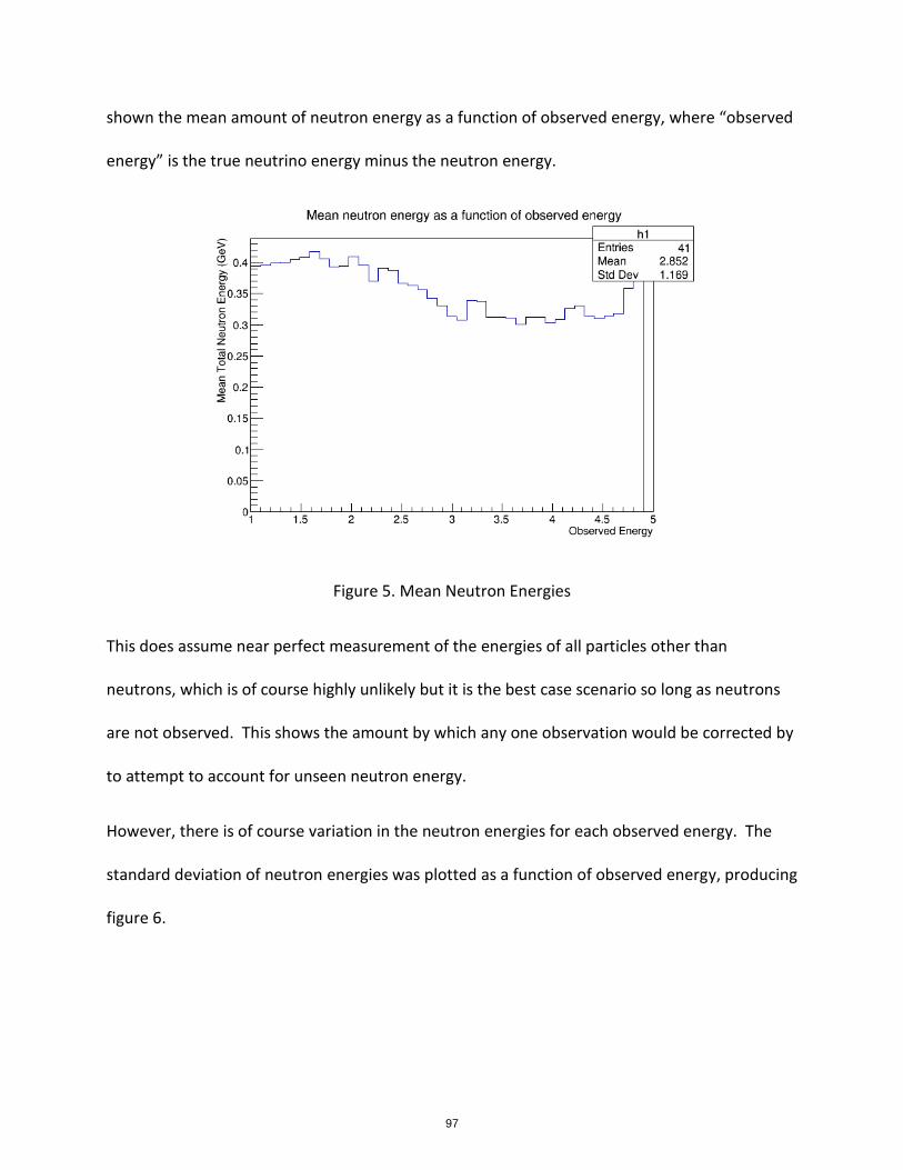
shown the mean amount of neutron energy as a function of observed energy, where “observed

energy” is the true neutrino energy minus the neutron energy.

Figure 5. Mean Neutron Energies

This does assume near perfect measurement of the energies of all particles other than

neutrons, which is of course highly unlikely but it is the best case scenario so long as neutrons

are not observed. This shows the amount by which any one observation would be corrected by

to attempt to account for unseen neutron energy.

However, there is of course variation in the neutron energies for each observed energy. The

standard deviation of neutron energies was plotted as a function of observed energy, producing

figure 6.

97

Figure 6. Standard Deviation of Neutron Energies

This shows that the standard deviation of the neutron energies for a given observed neutrino

energy are approximately 400 to 500 MeV. That is the uncertainty associated with the attempt

to account for unseen neutrons based on the simulation. This is very unfortunate for the DUNE

experiment, as these uncertainties are on the order of 15% to 20% of the energies of the typical

neutrinos.

We tried to get an idea for how damaging this would be by looking the resolution necessary to

study muon neutrino disappearance at around 2.5 GeV. This is the dip shown in Figure 1. As

mentioned previously, we did not initially have access to the approximate width of this dip.

Prob3++ was used to produce the following estimation of oscillation probabilities for muon

neutrinos staying muon neutrinos in the DUNE beam.

98

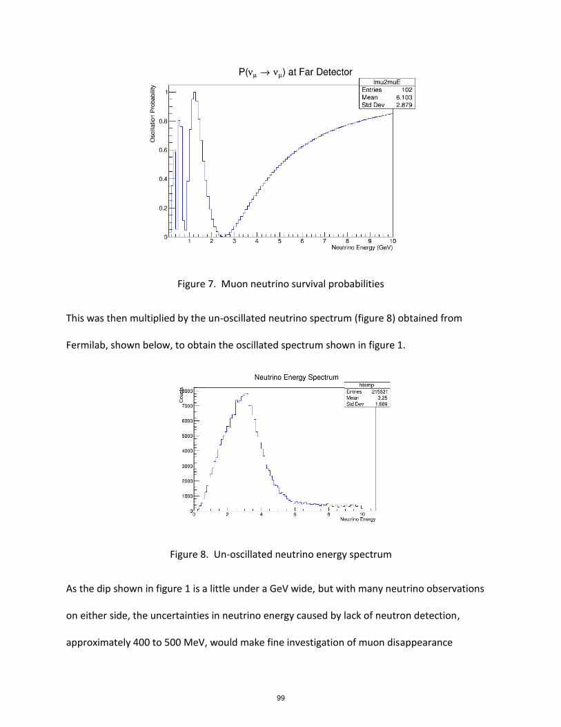
Figure 7. Muon neutrino survival probabilities

This was then multiplied by the un-oscillated neutrino spectrum (figure 8) obtained from

Fermilab, shown below, to obtain the oscillated spectrum shown in figure 1.

Figure 8. Un-oscillated neutrino energy spectrum

As the dip shown in figure 1 is a little under a GeV wide, but with many neutrino observations

on either side, the uncertainties in neutrino energy caused by lack of neutron detection,

approximately 400 to 500 MeV, would make fine investigation of muon disappearance

99

impossible. Events which belong on the left of the dip may be measured to be in the middle as

would events which belong on the right.

Conclusion:

Accurate energy reconstruction will be necessary for DUNE to study neutrino oscillations. Since

the DUNE detector will be a LArTPC, DUNE will have a weakness in measuring the energies of

neutrons. Simulations indicate that the amount of energy deposited in neutrons varies

significantly which prevents neutron energy being blindly accounted for from the simulation.

The resulting uncertainty in energy resolution will provide a serious challenge for the

experiment before it can accurately investigate neutrino oscillation and CP violation.

Acknowledgements and References:

Dr. LoSecco at Notre Dame for taking me as his research student and for his expertise in the

field.

Drs. Tom Junk and Tingjun Yang at Fermilab for their assistance in the use of Fermilab software.

Dr. Umesh Garg and the Notre Dame physics for providing this REU opportunity.

LBNF/DUNE Conceptual Design Reports Vols. 1 and 2: https://arxiv.org/abs/1601.05471

https://arxiv.org/abs/1512.06148

100

COMMISSIONING OF A FARADAY CUP FOR THE SOLENOID SPECTROMETER FOR NUCLEAR

ASTROPHYSICS (SSNAP)

EMMANUEL GARCIA

2017 NSF/REU Program Physics Department, University of Notre Dame

ADVISOR:

Dr. Dan Bardayan

101

Abstract

The Solenoid Spectrometer for Nuclear Astrophysics (SSNAP) is a HELIOS-like helical orbit

spectrometer being developed at the University of Notre Dame. Designed around position- sensitive

silicon detectors set along the axis of the second TwinSol solenoid, it will improve our capacity to study

nucleon transfer reactions. SSNAP will be sensitive to the charged light-ions produced in these reactions,

improving our ability to understand the created residual nuclei. The study of nucleon transfer reactions gives

us insight into many nucleosynthesis processes occurring in astrophysical events, such as novae bursts,

neutron-star collisions, among others. This work focuses on the design and construction of a Faraday Cup

detector that is part of recent developments of SSNAP. The preparation of titanium gas cell windows and

deuterated- polyethylene targets to be used in TwinSol experiments is also reported.

1. Introduction

In the early stages of the universe, in the span of the first 10 to 1000 seconds after the Big Bang, only

light nuclei up to lithium-7 were made [1]. Therefore, all the heavier elements that can be seen throughout the

universe have since been made through multiple astrophysical nucleosynthesis processes. Among these

we encounter neutron and proton capture processes, which open the door for the creation of a plethora of

isotopes that then decay into heavier stable elements.

Through the use of transfer reactions, we are able to study the nuclear structure of the nuclei created by

neutron and proton capture processes. By measuring the ejected light-ions produced by these reactions, we

gain valuable information about the residual nuclei [2]. Understanding the structure and characteristics of

these nuclei gives us insight into processes such as the s-process and r-process, and how they fit into our

models of the astrophysical phenomena that initiate them.

102

Since the installment of TwinSol in 1998, it has been used for numerous experiments

involving the use of Radioactive Ion Beams (RIB). A schematic of the current set-up is shown in Fig 1.

The use of RIBs allows us to study reactions encompassing short-lived nuclei that would be unsuitable for

targets since they would decay very rapidly. The RIBs produced by TwinSol are produced through the

In-Flight method, in which a stable ion beam bombards a gas target and produces a “cocktail” beam

with different nuclei, including the desired radioactive product [2]. The magnetic field of the solenoids is

then used to focus the desired radioactive nuclei and separate it from the rest of the contaminants. However,

since some of the nuclei share a similar momentum- to-charge ratio, and thus similar energies, it is

possible that some of the contaminants remain in the beam.

SSNAP consists of an improvement to the current TwinSol device by outfitting the second

solenoid as a helical spectrometer. This will broaden the scope of reactions in normal kinematics that can

be studied with the device as well as providing several advantages such as better particle identification

and large angular coverage.

A new Faraday Cup was commissioned as part of the SSNAP design in order to normalize the

data. The design, installation and testing of the device, as well as the preparation of titanium gas cell

windows and deuterated-polyethylene targets, is outlined in the present work.

Fig. 1. Schematic representation of TwinSol, located at the University of Notre Dame Nuclear Science Laboratory.

103

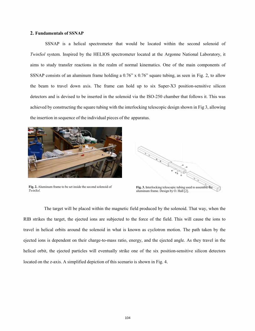
2. Fundamentals of SSNAP

SSNAP is a helical spectrometer that would be located within the second solenoid of

TwinSol system. Inspired by the HELIOS spectrometer located at the Argonne National Laboratory, it

aims to study transfer reactions in the realm of normal kinematics. One of the main components of

SSNAP consists of an aluminum frame holding a 0.76” x 0.76” square tubing, as seen in Fig. 2, to allow

the beam to travel down axis. The frame can hold up to six Super-X3 position-sensitive silicon

detectors and is devised to be inserted in the solenoid via the ISO-250 chamber that follows it. This was

achieved by constructing the square tubing with the interlocking telescopic design shown in Fig 3, allowing

the insertion in sequence of the individual pieces of the apparatus.

The target will be placed within the magnetic field produced by the solenoid. That way, when the

RIB strikes the target, the ejected ions are subjected to the force of the field. This will cause the ions to

travel in helical orbits around the solenoid in what is known as cyclotron motion. The path taken by the

ejected ions is dependent on their charge-to-mass ratio, energy, and the ejected angle. As they travel in the

helical orbit, the ejected particles will eventually strike one of the six position-sensitive silicon detectors

located on the z-axis. A simplified depiction of this scenario is shown in Fig. 4.

Fig. 3. Interlocking telescopic tubing used to assemble the aluminum frame. Design by O. Hall [2].

Fig. 2. Aluminum frame to be set inside the second solenoid of TwinSol.

104

&

2.1 Advantages of SSNAP

Once the particles are detected by the position-sensitive silicon detectors, three quantities are

measured by making use of the geometry of the system: the particle’s energy in the laboratory

frame 𝐸𝐸"#$, the position detected along the solenoid axis 𝑧𝑧&, and the Time-of-Flight (ToF) of the

ejected particle 𝑇𝑇()( . From these measured quantities, the angle of emission 𝜃𝜃+, and the energy

𝐸𝐸+, in the center-of-mass (CM) frame can be reproduced by the equations 𝜃𝜃+, = cos2&

& 56782349:;< CD;<EFGHI (𝑖𝑖) 𝐸𝐸(9 = 𝐸𝐸"#$ + 𝑚𝑚𝑉𝑉+, 3

− 9:RC8I SRTR (𝑖𝑖𝑖𝑖)

34 39=>?@A9B:;<B2

where the value of the CM’s velocity 𝑉𝑉(9 is fixed for a given beam energy and the magnetic field is fixed for the experiment.

Measuring the axial distance instead of the emitted angle provides its advantages by preventing

kinematic compression of the excited states at higher angles. This allows for clearer separation of the states.

It also allows for the full determination of the angular dependence of a reaction in one measurement [2]. In

addition, with the new set-up the detectors are kept out of the path of the beam, reducing potential damage and

providing large angular coverage.

Another advantage provided by SSNAP is easy particle identification. Since the orbital periods for

different particles varies as a function of their mass-to-charge ratio, particle identification can be obtained

by the ToF measurements. This is particularly useful for experiments

Fig. 4. Trajectory of the ejected ions after striking a target inside the solenoid. The ions will travel in a helical orbit until striking on of the six position-sensitive detectors located on the z-axis.

3

J

105

in which the particle energies are very low, as well as those that require high energy resolution, such as

Q-value measurements, where traditional methods such as telescope detectors are not ideal [2]. However, it

should be noted that this method is not without flaws; since various ions have the same mass-to-charge

ratio, they will have the same ToF.

3. Faraday Cup

3.1 Theory

A Faraday Cup (FC) is a conductive cup designed to catch charged-particles in a vacuum. When a

beam of ions hits the metal surface, the ions are neutralized while the cup gains a net charge. The FC

can then be discharged, producing a small amount of current which is measured by an electrometer

attached to the device. The amount of current measured is proportional to the amount of charge of the

incident particle, which is quantized. Therefore, by measuring the electric current flowing through the

metal cup, the number of ions being delivered by the ionized beam can be known. With proper

design, a FC can measure currents as small as 10−14A, which corresponds approximately to an ion

flux of 105 ions/s [3].

In order to get an accurate reading, care must be taken for backscattered ions or secondary

electrons that may be ejected from the cup when the ion beam strikes its surface. The escape of these

ions results in a current overestimation for positively charged ion beams and current

underestimation for negatively charged ones [4]. To avoid this problem, a suppressor with a negative

voltage is usually placed in front of the FC. This induces an electro-static field which pushes the stray

ions back to the cup.

106

3.2 Design Requirements

One of the requirements when designing the FC for SSNAP was the ability to be able to

assemble and disassemble it from the beamline with ease, since the solenoids are still to be used for

projects other than SSNAP. However, since it is to be placed in a chamber located after the solenoid,

this did not present the same challenges as the other components of SSNAP, which are to be placed

inside the solenoid and are therefore much more difficult to access and manipulate. Additionally, in

order to get a good alignment with the beam, it had to be able to have linear vertical motion while

limiting its rotational movement.

3.3 Design

Fig. 5 shows the mounted assembly of the FC. It consists of a cylindrical suppressor

attached by insulating ceramic cylinders to the cup. It is essential that the suppressor and the cup are

completely electrically isolated, otherwise voltage applied to the suppressor would impede the appropriate

functioning of the cup. The cup is enclosed by a tantalum plate which receives the direct impact of the

beam. Tantalum is characterized by its high conductivity and resistance to activation, making it an ideal

choice for the FC. The whole ensemble was mounted in an aluminum frame that allows for the attachment

to a linear drive. The linear drive consists of bellows of adjustable length, allowing suspension and

alignment of the FC along the beam axis.

An ISO-250 flange was modified to attach the linear drive by using a CF (ConFlat) seal. Two

BNC feedthroughs were also made in the flange for the suppressor and cup connections. Once the cup

is installed into the ISO chamber, as shown in Fig, 5c, it can be easily set-up or removed from the

beam axis by manipulating the actuator on the top of the chamber.

107

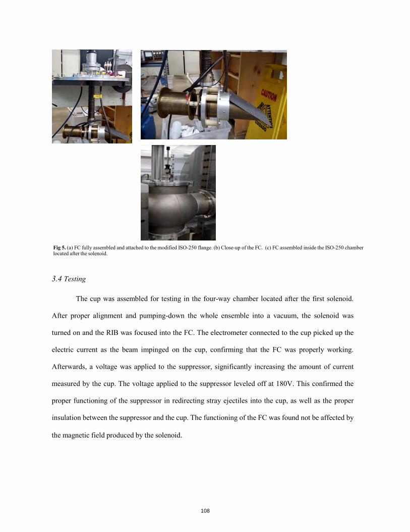
3.4 Testing

The cup was assembled for testing in the four-way chamber located after the first solenoid.

After proper alignment and pumping-down the whole ensemble into a vacuum, the solenoid was

turned on and the RIB was focused into the FC. The electrometer connected to the cup picked up the

electric current as the beam impinged on the cup, confirming that the FC was properly working.

Afterwards, a voltage was applied to the suppressor, significantly increasing the amount of current

measured by the cup. The voltage applied to the suppressor leveled off at 180V. This confirmed the

proper functioning of the suppressor in redirecting stray ejectiles into the cup, as well as the proper

insulation between the suppressor and the cup. The functioning of the FC was found not be affected by

the magnetic field produced by the solenoid.

Fig 5. (a) FC fully assembled and attached to the modified ISO-250 flange. (b) Close-up of the FC. (c) FC assembled inside the ISO-250 chamber located after the solenoid.

108

4. Gas Cell Windows

Many of the experiments carried out on the TwinSol facility involves the use of gas targets

such deuterium to create RIBs. The gas is contained in gas cells enclosed by thin titanium foils. The

foils have to thin enough so that the RIBs can pass through them with minimum scattering

and energy loss, but strong enough to withstand the impact of the beam and pressure of the gas without

breaking.

Following the procedure outlined in Ref. [5], circular and square titanium foils of initial

thicknesses 5𝜇𝜇𝑚𝑚 and 4𝜇𝜇𝑚𝑚 respectively were rolled with a rolling mill down to thicknesses of 3𝜇𝜇𝑚𝑚. We

found that the 5𝜇𝜇𝑚𝑚 circular foils produced a much better batch in comparison with the 4𝜇𝜇𝑚𝑚 square foils,

which were characterized by the presence of pinholes and lower reliability. It should be noted that the foils

degrade over time, so a fresh batch have to be made for each experiment.

5. Preparation of deuterated-polyethylene targets

Although many of the low-energy nuclear physics experiments done with TwinSol employ gas

deuterium targets for RIB production, some experiments benefit from the use of thin self- supported

targets containing deuterium. The most commonly used deuterium-containing target is deuterated-

polyethylene (C2D4) due to several favorable properties. It can be made into films with

areal densities ranging from tens of 𝜇𝜇𝑔𝑔/𝑐𝑐𝑚𝑚3 to several 𝑚𝑚𝑔𝑔/𝑐𝑐𝑚𝑚3. The thickness used requires a

compromise between reaction yield and target-induced energy broadening. Furthermore, it ensures

a favorable ratio (2:1) of deuterons to carbons, resulting in a favorable ratio of yield over energy loss.

Finally, due to the relatively low Z of carbon, extraneous stopping power is minimized [6].

Various C2D4 targets were prepared using the technique described by M. Febbraro, et al [6].

We used an alpha source of known energies to measure the energy loss of the alpha particles traversing

the film. The thickness of the films was then calculated using the known stopping power

of the alpha particles in C2D4. The films prepared had areal densities ranging from 192 𝜇𝜇𝑔𝑔/𝑐𝑐𝑚𝑚3 to

337𝜇𝜇𝑔𝑔/𝑐𝑐𝑚𝑚3, ideal for the energies used in our reaction studies.

109

6. Conclusions

The motivation and advantages of the helical spectrometer SSNAP were presented. The design,

construction and testing of a new Faraday Cup to be used with SSNAP was introduced. The FC tests

shows proper functioning in the measurement of current by the cup and the capture of stray ions by the

suppressor. The magnetic field generated by the TwinSol was found to not interfere with the functioning

of the FC. The preparation, uses and characterization of the titanium gas cell windows and deuterated-

polyethylene targets to be used with TwinSol and/or SSNAP was

presented. It was found that the 5𝜇𝜇𝑚𝑚 circular foils rolled down to 3𝜇𝜇𝑚𝑚 produced stronger and more reliable

windows than the square 4𝜇𝜇𝑚𝑚 foils.

7. Acknowledgments

I would like to thank Dr. Bardayan for having me as part of his team of researchers for the summer. I

would also like to thank Dr. Patrick O’Malley for his invaluable help getting the project done and his

patient and detailed explanations. Special thanks to Jerry Lingle for his help in designing the Faraday

Cup, as well as Jacob Allen, Matthew Hall and Gabriel Brown for their assistance. Finally, special

thanks Dr. Garg and the NSF for the hosting and funding of this REU program.

References

[1] Keith A. Olive, Gary Steigman, Terry P. Walker, Physics Reports 333-334 (2000) 389 URL: <https://doi.org/10.1016/S0370-1573(00)00031-4>. [2] O. Hall “The Design of SSNAP and the implementation on an ion chamber for the characterization of radioactive ion beams”, Master’s dissertation, University of Surrey, 2016. [3] Robert B. Darling, Adi A. Scheidemann, K.N. Bhat, T.-C. Chen, Sensors and Actuators A: Physical 95 (2002) 84 URL: < https://doi.org/10.1016/S0924-4247(01)00718-X>. [4] A. Kashefian Naieni, F. Bahrami, N. Yasrebi, B. Rashidian, Vacuum 83 (2009) 1095 URL: <https://doi.org/10.1016/j.vacuum.2009.01.005>. [5] J.P. Greene and G.E. Thomas, Physics Div., Argonne National Lab. PHY-8557-HI-96 (1997) URL: <http://www.iaea.org/inis/collection/NCLCollectionStore/_Public/28/018/28018315.pdf>. [6] M. Febbraro. D. Walter, S.C. Shadrick, S.D. Pain, K.A. Chipps, C. Thornsberry, E. Lesser, submitted for publication to Nucl. Intr. and Meth. A (2017) [Unpublished].

110

  

 Identification of candidate metal-poor stars  

from the HK survey by pruning with  the Gaia DR-1 data release 

  

       

Notre Dame Physics REU  

Jazmine Jefferson         

Advisors: Prof. Timothy Beers Prof. Vinicius Placco 

   

111

1. INTRODUCTION 

It is widely known that details regarding the evolution of the Universe can be 

gleaned from studying the chemical composition of stars. Astronomers have been 

utilizing this knowledge for decades, studying stars to piece together information on 

the intrinsic properties of the Milky Way, such as its structure and origin. The 

chemical composition yields information concerning a star’s formation era, since in 

their atmospheres, stars preserve information on the chemical and physical 

conditions of their natal clouds (Frebel et al. 2015). Studying the chemical 

composition of older, metal-poor stars has opened doors to a host of contemporary 

concepts in the field of astrophysics. This includes exploring the nature of the Big 

Bang and the nucleosynthetic processes that took place in the early Universe that 

lead to the formation of the first stars and galaxies.  

1.1 METAL POOR STARS 

Metal-poor stars are remnants of the early Universe. In its infancy, the 

Universe was composed of hydrogen and helium gases that compressed over a few 

hundred million years to form the very first generation of stars. These stars, 

denoted as population III stars, were massive and consequently lived short lives. In 

their death, these stars exploded into supernovae and dispersed the first metals 

into the interstellar medium. Population II, or metal-poor, objects are those with 

very low levels of metal relative to our Sun and were formed from the clouds of the 

first generation of stars. Population II as well as all subsequent generations of stars 

formed from chemically-enriched material from the previous generations’ 

112

nucleosynthetic processes. Metal-poor stars are therefore the oldest stars in the 

Universe and contain information about the chemical composition of their 

progenitor clouds in their atmosphere; these stars primarily exist in the inner and 

outer halo substructures in the Milky Way. 

  Stars are classified according to their abundance of metals (defined by 

astronomers as elements heavier than He) relative to our Sun. The abundance of an 

element uses the notation  , where NA and NBA/B] ≡ log (N /N )∗ −log (N /N )[ 10 A B 10 A B  

denote the number of atoms of elements A and B. Fe has traditionally been taken 

as a reference element to enable comparisons of the metallicity of one star with 

another, quantified as [Fe/H] (Beers et al. 2005). Metal-poor stars are classified as 

having a metallicity [F/He] < -1. A table of metallicity nomenclature as suggested 

by Beers et al. follows.

 Table 1 Metallicity nomenclature suggestions by Beers et al. (2005) 

 1.2 CEMP STARS 

Metal-poor stars with high carbon to iron ratios are considered 

carbon-enhanced. Carbon-enhanced metal-poor stars (CEMP) stars are defined by 

Beers et al. to have a carbon to iron abundance ratio [C/Fe] of > +1.0. The fraction 

113

of metal-poor stars that are carbon-enhanced increases at lower metallicities. 

CEMP stars constitutes roughly 20% of metal-poor stars with [Fe/H] ≤ -2.0 while 

only a few percent of stars similar to the Sun are carbon-enhanced. The prevalence 

of CEMP stars at lower metallicities suggests that the chemical composition of the 

Universe had higher levels of carbon at the time of the star formation. Examples of 

current theories that explain this abundance of carbon include: a primordial process 

from massive progenitor stars, internal production from low mass, extremely 

metal-poor stars, or production from stars of intermediate mass, which was then 

transferred to a lower mass companion (Beers et al. 2005). 

  CEMP stars are further divided into subclasses based upon their neutron 

capture processes. Heavy nuclei beyond Fe are produced through neutrons merging 

with nuclei in high-energy astrophysical sites such as supernovae and neutron-star 

mergers. The subclasses of neutron capture for CEMP stars are depicted in Table 2. 

 

 Table 2 Definition of subclasses of CEMP stars 

 Most heavy elements can only form in a rapid neutron capture, or r-process. 

R-process occurs when neutrons are captured more rapidly than the rate of beta 

114

decay. Similarly, s-process, or slow neutron capture, occurs when neutrons are 

captured at a slower rate than that of beta decay. Eu is used as a reference element 

because its abundance is one of the most readily available spectra to measure in 

metal-poor stars. It is necessary and useful to distinguish stars with “pure” r- or 

s-processed elements and stars that have element abundances with both, known as 

r/s-processed. CEMP stars with no strong overabundances of either r- or s-processed 

elements are dubbed CEMP-no stars.  

2. SURVEYS OF THE STARS 

2.1 HK OBJECTIVE PRISM SURVEY 

In 1978, George Preston and Steve Shectman of the Carnegie Observatory 

performed a survey in an effort to identify candidates for metal-poor stars in our 

Galaxy. This survey made use of an objective prism plate and an interference filter 

to successfully isolate CaII H and K lines and obtain low-resolution spectra of stars 

several magnitudes fainter than previously achieved (Beers 2015). Roughly 60 

plates were visually scanned and followed up with medium-resolution spectroscopy 

for further analysis by Beers (Beers et al. 1985). 

  This survey was expanded by Beers with 240 additional prism plates from 

the northern and southern hemisphere using the Curtis and Burrell Schmidt 

telescopes. Each HK plate contains thousands of low-resolution spectra that were 

visually scanned to find the best metal-poor candidates; a large fraction of these 

plates have been followed up with medium-resolution spectroscopies.  

2.2 GAIA-ESO SURVEY 

115

The Gaia mission is to allow astronomers to investigate the origin and 

subsequent evolution of the Milky Way through providing an accurate astronomical 

census of over 1 billion stars. The first data release in 2013, DR-1, contained 

astrometric parameters and the average photometry from 1.14 billion stars 

surveyed in its first six months of operation (Mora et al. 2017). Stellar parameters 

logged in DR-1 include information on parallax, proper motions, distances from 

stars down to magnitude V = 20. The release has been made public and is readily 

available for cross-matching with other surveys.  

3. IDENTIFYING CANDIDATE CEMP STARS 

3.1 HK PLATES 

The HK telescopes surveyed 2800 deg 2 and 4100 deg 2 of the northern and 

southern hemisphere, recording widened objective-prism spectra of up to thousands 

of stars at once. Prints of the plates were visually scanned with a 10-X microscope 

for CaII H and K lines in search for metal-poor candidates. Figure 1 illustrates the 

appearance of these lines as seen by the classifier. 

 Figure 1 Illustration of appearance of CaII H and K lines as seen by visual 

classifier (Beers 2017)  

116

  Candidates of metal-poor stars as well as stars used for calibration of the 

coordinate system were marked and indexed by hand onto the plate prints. An 

example of one of these prints is shown in Figures 2 and 3. 

                              

  The positions of the targets from the HK survey are relatively inaccurate, 

with some plates having over 10 arcseconds of error. The curvature of the telescope 

lens also creates a parabolic fit onto the plate and further distorts the coordinates of 

the targets. To obtain more accurate positions of the stars, .fit files of each 

individual target were created and analyzed through SAOImage DS9. Right 

ascension and declination in decimal degrees were logged for roughly 14,000 

targets. The updated coordinates were uploaded to Centre de Données 

astronomiques de Strasbourg (CDS) X-match Service to crossmatch HK targets to 

stars obtained from Gaia DR-1. 

3.2 ANALYSIS  

117

Data compiled from the CDS X-Match Service included photometry and 

information on astrometric parameters such as the parallax, proper motions, and 

distance from the galactic center in addition to the positions of each candidate. The 

catalogue of candidates are then pruned to locate those most likely to be CEMP 

stars. Stars in the foreground of the survey are those within the galactic disk and 

are therefore less likely to be metal-poor. To increase the efficiency of locating 

CEMP stars, calculations were made to locate stars above the galactic plane ( Z ).  

Z = dsin(b) (1) 

Where d denotes distance from the galactic center,  b  denotes the galactic 

latitude, and  µ denotes total proper motion that is used in calculating the 

transverse velocity; metal-poor stars exist primarily in the halo system and will 

consequently have higher relative transverse velocities. 

V T = 4.74µd (2)  

4. RESULTS AND CONCLUSIONS 

4.1 RESULTS 

The CDS X-match service successfully matched roughly 1200 stars with all 

necessary data for calculations. Many of the candidate stars have been observed 

since the HK selection process; stars that have been observed were logged. Stars 

were further classified according to their metal-poor candidacy, with 1 being best.  

118

 

Figure 4 Plot of all HK stars (black) and stars of classes I-IV Z vs V T that have been observed 

 

Figure 5 Plot of all HK stars (black) and stars of classes I-IV  Z vs V T that are not yet observed 

 Plots of the stars’ distances from the galactic plane as a function of their transverse 

velocities is ideal for quickly eliminating foreground objects as candidates. The face 

of the plot is color-coded according to the positions and transverse velocities of both 

the halo and disk of the Galaxy. The stars remaining in the HK survey will undergo 

a similar identification process before both sets of data will have metallicities 

119

assigned. The success rate of finding CEMP stars through the reported pruning 

method will then be determined.  

REFERENCES 

Beers, T. C. et al . The Discovery and Analysis of Very Metal-Poor Stars in the Galaxy. Annual Review of Astronomy and Astrophysics 43, 531–580 (2005).  Beers, T. C. Back to the Future: The Calcium HK Survey of Beers, Preston and Shectman. Fifty Years of Wide Field Studies in the Southern Hemisphere: Resolved Stellar Populations of the Galactic Bulge and Magellanic Clouds  491,140 (2015).  Frebel, A et al . Near-Field Cosmology with Metal-Poor Stars. Annual Review of Astronomy and Astrophysics (2015).  Mora, A et al . The Gaia Archive. Astrometry and Astrophysics in the Gaia Sky. Proceedings IAU Symposium No. 330 (2017).  Beers, T. C. “The Oldest Stars.” Astrophysics Update 2 , Springer Berlin Heidelberg, 2017.  Beers, T. C., Preston, G. W., & Shectman, S. A. 1985, AJ, 90, 2089 

120

Determining the Effect of Stellar Evolution on Carbon Abundances

David Kalamarides

University of Notre Dame Email: dkalamar@nd.edu

Carbon-Enhanced Metal-Poor (CEMP) stars are believed to be the direct descendants of the first generation of stars to be formed in the universe. Detailed chemical abundances of CEMP stars are important inputs for theoretical models, and the effects of stellar evolution on some of these abundances must be accounted for. Since the carbon content of these stars can decline as they age, it is necessary to correct observed measurements back to the initial conditions. We have refined the procedure for which we estimate corrections for carbon and nitrogen abundance ratios ([C/Fe] & [N/Fe]) from a large sample of observed stars from the Sloan Digital Sky Survey. After adjusting the models to match the observed data, new estimations were made from a Locally Weighted Scatterplot Smoothing (LOESS) regression function, which estimates [C/Fe] & [N/Fe] from a number of other parameters that are easier to identify in stars, such as surface gravity, effective temperature, and metallicity. An online tool was created so the

public can run these calculations for any data.

Received 10 August 2017

1. INTRODUCTION

Metal-poor stars, especially those with high concentra- tions of carbon, have been identified by recent studies to be central to the understanding the chemical evolution of our galaxy.

Carbon-Enhanced Metal-Poor (CEMP) stars are classified as having a low iron-to-hydrogen (i.e. [Fe/H] < -2.0) and a high carbon-to-iron ratio (i.e. [C/Fe] > +1.0) [2]

CEMP stars can be subdivided based on the source of their enrichment. CEMP star whose heavy elements were produced by r-process are classified as CEMP-r stars and identified by [Eu/Fe] > +1. Enrichment can also come from a mass transfer by a binary red-giant. These stars are classified as CEMP-s stars and identified by [Ba/Fe] > +1 and [Ba/Eu] > +0.5. When 0 < [Ba/EU] < +0.5, the CEMP star can be enriched by both r- and s- processes and classified as CEMP-r/s.[2] The final classification of CEMP stars are those whose enrichment must have come from carbon abundant natal gas clouds.

In this paper, we revisit the depletion of surface carbon abundances occurring in CEMP-no stars during the upper red-giant branch stage of evolution as originally done in Placco et Al. 2014 [6]. Figures 1 and 2 demonstrate the depletion of carbon and

enrichment of nitrogen as CN processing occurs. Using the same stellar evolution models [3], we improve the accuracy and efficiency of the online calculator as well as add [N/Fe] to the stellar parameters used to calculate these carbon corrections. In addition, we now provide corrections for the change in surface nitrogen that occur concurrently with the carbon depletion.

This paper is structured as followed. Section 2 discusses the original work, Placco et Al. 2014, which this work is correcting. It outlines the original procedure and the errors that it faced. Section 3 discusses the new procedure which successfully corrects for both carbon depletion and nitrogen enhancement in the red-giant branch. Section 4 analyzes the possible errors. We discuss the online calculator and our results in Section 5.

2. ORIGINAL WORK

Placco et Al (2014) began by creating an array of models using the STARS stellar evolution code [3]. This array set parameters for metallicity, carbon, and nitrogen abundances. [Fe/H] was set to -1.3, -2.3, - 3.3, and -4.3. [C/Fe] ranged from -1.0 to 3.0 in steps of 0.5. [N/Fe] ranged from -1.0 to 2.0 also in steps of 0.5. These models were then evolved through the pre main-sequence to the end of the red-giant branch.

121

FIGURE 1. The carbon abundances of simulated stars against log g show the depletion of carbon through the red- giant branch. [Fe/H] is held at -1.3 and [N/Fe] at 0.0.

FIGURE 2. The nitrogen abundances of simulated stars are shown against logg. [Fe/H] is held at -1.3 and [C/Fe] at 0.0. The spike in nitrogen is due to the CN processing.

Placco et Al then collected a sample of metal-poor stars with high-resolution spectroscopies from the most recent SAGA database [7] and data assembled by Frebel et Al (2010)[5]. Stars which had already been identified as CEMP-s or CEMP-r/s were excluded from this data. After comparing the literature data and the observed, Placco et Al noticed a disparity between the surface gravity of the two. Log g was shifted in all models by 0.5 to account for this difference.

Placco et Al.’s method for correcting carbon depletions is as follows. They began by taking four of the simulated models: those with the closest metallicity [Fe/H] and carbon abundance [C/Fe]. Surface gravity (log g) and nitrogen (N/Fe) were matched as closely as possible. The appropriate correction for each of these models was then determined. The final correction was calculated through a linear interpolation of these four models. This method is vizualized in figure 3

This method ran into two main issues. First, any star outside of the simulated models’ original parameters

FIGURE 3. Procedure use in Placco et al (2015) [6]. Each vertical line represents the correction for a certain chosen model. The final correction is interpolated from these four lines.

(i.e. [Fe/H] > -1.3 or < -4.3, [C/Fe] > 3.0 or < -1.0, or log g > 4.5 or < 0.3) would have an increasing potential error the further it was from the models. In other words, this method could accurately interpolate, but could not extrapolate. Second, nitrogen abundances were rounded off to the nearest 0.5, causing a large increase in uncertainty. In addition, the change in nitrogen as a function of change in surface gravity through each model’s evolution is entirely ignored. It is for these two reasons that we create a new procedure for calculating both carbon and nitrogen corrections.

3. PROCEDURE

To predict the changes in carbon and nitrogen, we use two locally weighted scatter plot smoothing (LOESS) regression models[4]. These models take a least squares regression from subsets of data of the stellar models from the STARS Stellar Evolution code [7], that is it fits a curve to minimized the uncertainty for each data point in the subset. These subsets are parameterized by a certain span set for each model. This span is for the carbon correction model and for the nitrogen. Then once given the observed parameters of surface gravity (log g), iron abundance ([Fe/H]), carbon abundance([C/Fe]), and nitrogen abundance (Ne/Fe), we predict the changes in carbon and nitrogen through the two LOESS regression curves. Figures 7 and 8 depict the calculated corrections for a grid of given parameters.

4. UNCERTAINTY

1000 points of sample data to test the carbon and nitrogen corrections were randomly selected from the simulated models. Seen in figure 4, the carbon corrections are calculated for each point and compared. Figure 5 shows the distribution of error between the calculated initial carbon abundance and the set parameter for initial carbon. The mean error is 8.663116e-4 with a standard deviation of 1.649867e-2. Nitrogen similarly has a mean error of 6.076169e-4 and

122

FIGURE 4. Carbon abundance corrections for sample data. Black squares indicate the observed carbon. The red lines represent the calculated correction while the green triangles show the final returned carbon abundances.

FIGURE 5.

a standard deviation of 7.187593e-2. This sample indicates that calculations indeed match

the simulated models from the STARS evolution code.

5. CONCLUSIONS

This new method for calculating corrections for carbon and nitrogen though the red-giant branch allows for further work to occur with increased accuracy. One subject in particular that will benefit from these

updated corrections is the estimated frequency of carbon enhanced stars within our galaxy. These frequencies are vital as inputs for chemical evolution models of our galaxy. In addition, stars with carbon abundance slightly less +1.0 than can be confirmed as CEMP-no stars. There have been disputes over whether the lower limit to classify stars as carbon enhanced or not should be at +1.0 or +0.7 [1], as many stars between the range of these numbers exhibit properties of CEMP stars. It is likely that when carbon depletion is accounted for, it will be revealed that these stars were indeed carbon-enhanced at their creation. One star from the literature data that was processed in Figure, CS30322-023, has an observed carbon abundance of [C/Fe] = 0.67, but a calculated initial carbon abundance of [C/Fe] = 1.688. This drastic shift indicates that many stars that previously were ignored ought to be considered for CEMP frequencies within our galaxy.

In order to allow these future studies to occur, we

have also created an online tool so anyone may correct their observed carbon and nitrogen measurements. The tool takes all needed parameters in through an uploaded .csv file, and processes them through an Rscript running on the server’s terminal.

123

FIGURE 6. Carbon abundance corrections for literature data[5, 7]. Red squares indicate the observed carbon. The black lines represent the calculated correction while the green circles show the final returned carbon abundances.

6. FINAL THOUGHTS

This paper represents the culmination of my summer research with the University of Notre Dame’s summer Research Experience for Undergraduate program. Additional work is still required to smooth the nitrogen corrections, prepare this paper for publishing, and releasing the public online tool. Since I am still a Notre Dame student, I will continue to work on these three projects in the coming semester.

While re-designing a method for correcting carbon and nitrogen was the main project I independently worked on, I also assisted in three other projects. First, I compiled a pipeline from UVES, a high resolution spectrograph of the Very Large Telescope (VLT) array located in Cerro Paranal, Chile. Throughout the summer, I was then responsible for reducing spectrum for which the Galactic Archeology team needed. Second, I assisted in creating the GQ index, an updated for calculating the carbon abundances in stars by integrating over the g-band in an observed spectrum. This is an improvement on the previously used GP and GPE indices as this new method first subtracts out any dip in flux in the g-band found in spectra of stars with near-zero carbon. Third, I have begun work on developing a pipeline for the South African Large telescope. This data reducing program will allow other astronomers from all over the world to analyze working spectra from this telescope.

Finally, the online web tool should be published at

https://www3.nd.edu/ vplacco/carbon-cor.html within the coming year, dependent on the Office of Information Technologies’ clearance to add back-end processing to Dr. Vinicius Placco’s web page.

REFERENCES

[1] Aoki, W., Beers, T. C., Christlieb, N., et al. 2007, ApJ, 655, 492

[2] Beers, T. C., & Christlieb, N. 2005, ARA&A, 43, 531 [3] Eggleton, P. P., Tout, C., Pols, O., et al. 2011,

Astrophysics Source Code Library, ascl:1107.008 [4] Cleveland, W. S. , Grosse, E. and Shyu, W. M.

(1992) Local regression models. Chapter 8 of Statistical Models in S eds J.M. Chambers and T.J. Hastie, Wadsworth & Brooks/Cole.

[5] Frebel, A., Kirby, E. N., and Simon, J. D. 2010, Natur, 464, 72

[6] Placco, V. M. et Al (2014). Carbon-Enhanced Metal- Poor Star Frequencies in the Galaxy: Corrections for the Effect of Evolutionary Status on Carbon Abundances. Astrophysics Journal, 797, 21

[7] Suda, T., Katsuta, Y., Yamada, S., et al. 2008, PASJ, 60, 1159(Page 19).

124

FIGURE 7. [C/Fe] correction map for log g = 3.0, 2.0, 1.5, and 1.0 with [N/Fe] fixed at 0.0

125

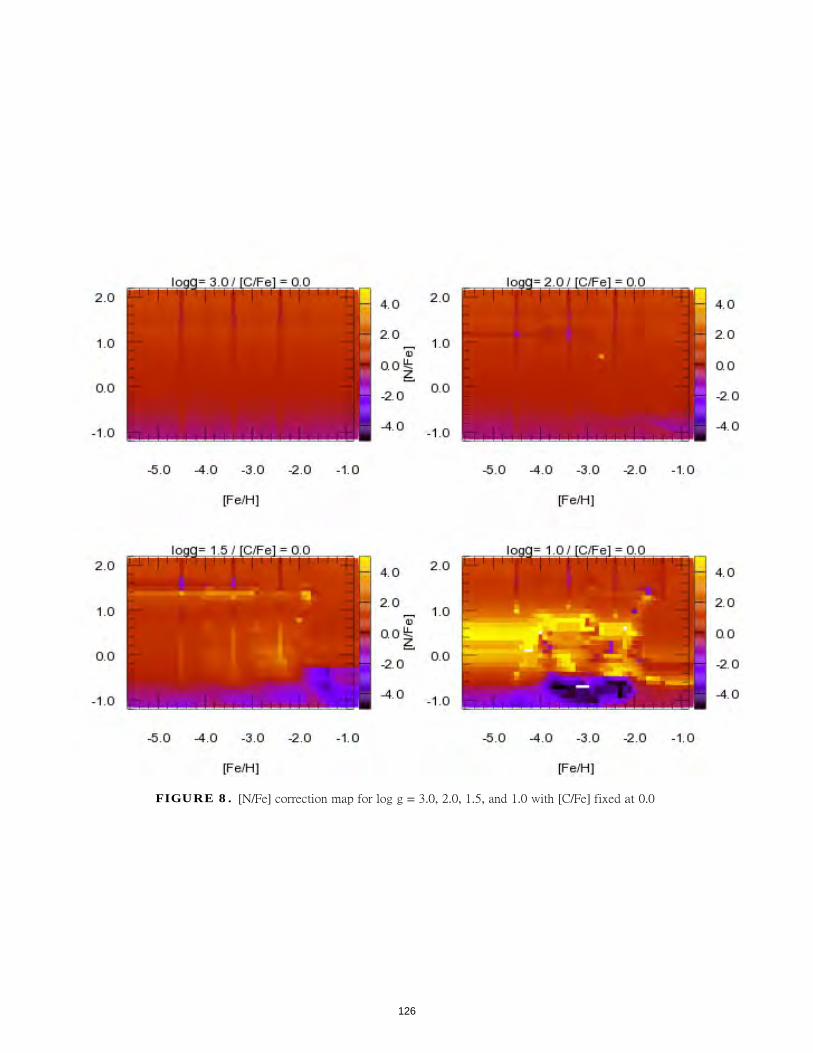
FIGURE 8. [N/Fe] correction map for log g = 3.0, 2.0, 1.5, and 1.0 with [C/Fe] fixed at 0.0

126

Analysis of Colonial Paper Currency

Michael Kurkowski, Catherine Cangany, Louis Jordan, Khachatur Manukyan, Zachary Schultz,

Michael Wiescher

Abstract

This project entailed studying the cellulose in paper, the ink, colorants, and other

materials used to produce American colonial currency. The technique primarily used in this

project was X-Ray Fluorescence Spectroscopy (XRF). XRF mapping was used to provide both

elemental analysis of large-scale objects as well as microscopic examination of individual

pigment particles in ink, in addition to the inorganic additives used to prepare paper. The

combination of elemental mapping with Fourier Transform Infrared (FTIR) and Raman

Spectroscopies permits an efficient analysis of the currency. These spectroscopic methods

help identify the molecular composition of the pigments. This combination of atomic and

molecular analytical techniques provided an in-depth characterization of the paper currency on

the macro, micro, and molecular levels. We have identified several of pigments that were used

in the preparation of inks and colorants. Also, different inorganic crystals, such as alumina-

silicates, have been detected in different papers. The FTIR spectroscopy allowed us to

determine the type of cellulose fiber used in the production of paper currency. Our future

research will be directed toward revealing important historical relationships between currencies

printed by different printers throughout the colonies.

Introduction

Throughout the eighteenth century, paper making was a growing profession.

Standardized currency in the American Colonies did not exist yet, so individual printers

127

purchased their paper from paper mills in the same way as everyone else. Original paper

manufacturing methods involved linen and cotton rags as the raw materials. Not until late in

American colonial times were mica crystals used in banknote paper production as an anti-

counterfeit strategy. 1

Once printers had the paper, they needed to turn it into viable currency. The very first

bills were printed by the Massachusetts Bay Colony to prevent bankruptcy due to military

expeditions. Without any tough-to-replicate designs, bills were relatively quickly and easily 2

counterfeited. One of the first printers to establish anti-counterfeiting methods was Benjamin

Franklin, with ink designs from leaves. Another common technique to prevent counterfeiting

was interspersing small mica crystals throughout the banknote paper.

Our method of analysis involved XRF Spectroscopy, which bombards a sample with a

beam of x-rays. The secondary x-rays produced by the sample are specific to the elements

within it; thus, the energies detected from the secondary x-rays identify the elements producing

them. This was very useful in identifying the composition of many of the written inks,

especially red ink.

FTIR spectra were taken on each of the currency bills to confirm the XRF spectra and to

detect lighter elements (additives, etc.) that were undetectable by XRF. It was also used to

confirm the presence of mica crystals in certain papers. FTIR is a technique similar to XRF, but

uses a different electromagnetic wavelength. It shines a beam of infrared light at the sample,

and detects the resultant energy produced by the vibration of the molecules.

One of the inks that couldn’t be fully analyzed by just XRF due to the presence of lighter

elements was the printed black ink. To confirm the existence of carbon (which is expected to

be found in bone black ink), I performed Raman spectroscopy on the bills, and found the

characteristic carbon peaks. Raman is a sister technique to FTIR, the difference between them

being that Raman shines a different wavelength of light: visible light (a red laser).

American Paper Mills, 1690‑18321

https://www.uscurrency.gov/content/history-american-currency2

128

To this end, the project was born, and was mostly conducted during the months of

June and July 2017 at the University of Notre Dame.

Data & Findings

Over the eighteenth century, the additives used in banknote paper changed depending

on the source the currency printers used. One notable difference can be seen in the New

Jersey graphs (top right), in which the paper contained an additive that manifested itself for

only a couple of years, 1762-1765. This same additive can also be seen in the Pennsylvania

graphs (top left) immediately after Franklin stopped printing currency, from 1769-1772, shortly

after New Jersey. Other more subtle changes in the paper can be seen, which give deeper

insight into currency printing and paper making methods of the time.

FTIR scans of paper over the years: Pennsylvania (top left), New Jersey (top right), Continental Currency (bottom left), and New York (bottom left).

129

Conclusion

The ability to use all three techniques, XRF, Raman, and FTIR, allowed us to gain a new

insight into the ways currency was produced in the colonies throughout the eighteenth century.

XRF single-point analysis gave clearer knowledge as to the contents of banknote ink, providing

a map of the contents of the various inks used in the production of a single bill of currency.

Coupling this technique with Raman and FTIR allowed us to verify the data the XRF gave us,

and to see the history and progression of materials used alongside with the full contents of

each single currency.

This project promises to yield new results and better insight into colonial currency

making, with a more detailed analysis of the spectra and data taken over the course of this

summer. At the end of the project, there will be a physics database of one of the Library’s

special collections, and a confirmation of historical literature.

Acknowledgements

I would like to thank the Institute for Scholarship in the Liberal Arts, University of Notre

Dame, for making this project possible by its support from the Da Vinci Grant. I would also like

to thank the College of Science, University of Notre Dame, for hosting the 2017 Physics REU,

and its support otherwise in this research endeavor.

130

The use of RF carpets in Helium gas

Keenan Lambert - July 26, 2017

131

1.Introduction

The use of Radio-Frequency (RF) carpets in nuclear physics laboratories has been proven to be

an effective means of transporting ions. Low energy nuclear physics programs use large RF carpets to

transport ions in large volume gas cells. These cells are used to thermalize the fast-radioactive ion beam

produced in flight, such that they can later either be used in precision experiment or reaccelerated. Gas

cells are usually linear however a circular cyclotron gas stopper as been developed at the National

Superconducting Cyclotron Laboratory of MSU. The RF carpets in those gas cells vary in size and design

and can either be linear or circular. However, they all serve a similar purpose: to prevent the loss of ions

and guide ions to an extraction orifice connecting to an ion guide and a beam line where the ion beam is

transported at low energy.

The REU project presented in this report aimed at improving the RF carpet test setup in use at

the University of Notre Dame by adding a circuit to allow a traveling wave to be implemented onto the

RF carpet in addition to the RF. After this was accomplished the transport efficiency under various

conditions was studied.

2.Working principle of a RF carpet

RF Carpets are formed by a series of co-centric conductive rings on which an alternating potential

(in the radio-frequency range) is applied with opposite polarity on adjacent rings resulting in a strong

repelling force that keeps the ion a certain distance from the carpet. The traditional method of

transporting the ions consists of superimposing a potential gradient along the segments to drag the ions

towards the desired direction. A more recent method, called ion surfing, replaces the potential gradient

with a traveling wave, which is a signal at a lower frequency. The traveling wave is generated by

applying a sinusoidal potential phase-shifted by 90 degrees on adjacent electrodes and shown on Figure

132

1. This figure also shows schematically describes how the combination of both signals results in the

repulsion and transport of the ions by the carpet.

Figure 1: Schematic of a RF carpet used in the “ion surfing” transport method. The two opposite RF

phases are indicated by colors red and blue. A plate situated above the carpet and biased at a higher

potential Vp brings the ions down to the carpet. From Figure [1].

The RF carpet test setup at Notre Dame is comprised of one such carpet as well as a surface ion

source that produces potassium ions. The ions are first attracted by an electric field produced by the

potential difference between the ion source and a plate underneath it, which serves as an anode that pulls

them out. Then, the voltage difference (Vp in figure 1) between the plate and the carpet creates an electric

field, which pushes ions onto the RF carpet. An outer ring electrode around the edge of the carpet is used

to collect ions that are transported either using the travelling wave or simply by diffusion. The ions

transported are measured as an electrical current. The higher the current, the more ions are being

transported. However, some ions will splatter onto the carpet. Finally, if more charge is being dumped

on the carpet, it will start to screen the alternating RF field creating more ion loss. The possibility of

such space charge effect has been studied and will be presented in this report.

133

3. Generating alternating sin waves

For the travelling wave signal to be transposed onto the RF carpet, it is important to first generate

a signal and split it into four different phases and feed them to the corresponding electrodes (see figure

1). As shown in figure 1 each phase is shifted by ninety degrees with respect to the phase of the adjacent

electrode. As part of my REU project, I created such circuit using a fast-operational amplifier (op-amp),

capacitors, resistors, and potentiometers. The zero and 90 degrees LF phases where generated out of a

dual output arbitrary function generator (AFG). To produce the 180 and 270 degrees phases, we fed

these outputs to a phase inverting op-amp circuit such as the one shown on the left-hand side of Figure

2. The op-amp where also used to increase the amplitude of the signal produced by the AFG. Hence the

zero and 180 degrees phases where also sent to a non-inverting op-amp circuit like the one on the right-

hand side of Figure 2.

Figure 2: (left) Inverting op-amp circuit and (right) non-inverting op-amp circuit used to produce the

traveling waves. Figures from [2].

134

Figure 3: Photo of the op-amp circuitry used to produce the four phases of the traveling wave signal.

The circuit (Figure 3) includes potentiometers to adjust the amplitudes of the low frequency from

each op-amp to be equal to each other on the various RF carpet stripes, and to compensate for any

unforeseen surges from the RF signal.

Figure 4: Photo of the of the new RF circuit that combines the RF signal with the traveling wave

connected to the ultra-high vacuum feedthroughs that leads to the RF carpet inside the vacuum chamber.

135

Finally, the RF signal, provided by an RF amplifier, had to be impedance-matched to a resonant

circuit in which the RF carpet is the conductive part. This was accomplished using a transformer with

only one turn of a copper tube on the secondary side and 9 turns of copper wire on the primary side. The

secondary part of the circuit also naturally creates the 0 and 180 phases of the RF signal. In order to

combine the RF signal with the traveling wave, we had to add capacitors for the coupling and inductors

to prevent the RF from leaking toward the AFG providing the wave signal. Figure 4 shows a photo of

the new circuit.

4.Testing the carpet for efficiency

There are many parameters that can be changed to study the transport efficiency of an RF carpet.

These include: the RF amplitude and frequency, the travelling wave amplitude and frequency, the electric

field pushing the ions to the carpet, the gas pressure, the ion current, and the mass of the ion. In our

study, however, several parameters were held fixed: we used a gas pressure of 60 mbar, potassium ions,

and a RF of 12.3 MHz. Hence, only the RF amplitude, the ion beam current, and the wave amplitude

and frequency were varied.

The efficiency was determined by dividing the total current going to the carpet by the current

transported all the way to the outer ring. The total amount of current hitting the carpet in the absence of

RF and travelling wave was measured directly using a high-precision electrometer that can measure sub-

pA. Throughout our studies we kept the current hitting the carpet to be 100 +/- 1 pA. This was achieved

by changing the ion source potential for a given voltage on the plate above the carpet.

5.Experimental Results

The effects of varying the RF amplitude for different wave speeds is shown in Figure 5. As the

amplitude of the traveling wave Vw increases, there is a noticeable drop in efficiency. This is especially

136

true when Vw is increased from 3V to 5V, when a large drop in efficiency is observed. This could be

attributed to the ions getting closer to the carpet as Vw increases, resulting in more of them hitting the

carpet due to collision with helium atoms. The efficiency is also increasing with larger RF amplitude

(given here in terms of the RF generator gain in %). This is because at low RF amplitude the ion is less

affected by the oscillating potential that kicks it away from the carpet, resulting in a lower transport

efficiency. Finally, it is interesting to observe how at low RF amplitudes, having a traveling wave is

mandatory to observe transport efficiency. This might be due to the traveling wave being able to carry

the ions faster along the carpet, hence reducing the chances of a collision that would direct them towards

the carpet.

Figure 5: Variation of the RF carpet transport efficiency as a function of the gain of the RF generator

used for a 10 kHz wave and a potential of 60 V on the plate. The curves of different colors indicate the

amplitude of the traveling wave used. e.g. Vw1 is related to a 1 V wave and Vw0 to no wave.

137

The graph in Figure 6 illustrates how the RF carpet is able to maintain efficiency at higher Vw

amplitudes when the frequency of the Vw is also increased. The higher frequency carries the ions

faster above the carpet, allowing a larger Vw to be used.

Figure 6: Variation of the RF carpet transport efficiency as a function of the traveling used for 38%

gain and a potential of 60 V on the plate. The curves of different colors indicate the frequency of the

traveling wave used.

Figure 7 shows how the electric field pushing the ions from the source has an effect on the

transport efficiency. As the plate potential is increased, the ions feel a stronger force Fp pushing them

towards the carpet (see Figure 1). At a certain point the repelling force from the RF carpet FRF cannot

sustain it anymore and a loss in efficiency is observed. We also looked at the effect of increasing the

ion beam current hitting the carpet from 10 pA up to 1 nA. Having a traveling wave of 3 V has a

positive effect on the efficiency for 10pA, 100pA, and 1000pA currents. Increasing the ion source

current from 100 pA to 1000 pA does not seems to have an effect ion the transport efficiency. The

138

efficiency at 10 pA appears to be lower, but it should be noted that there is also a larger uncertainty due to the measurement process.

Figure 7: Variation of the RF carpet transport efficiency as a function of the potential on the plate for

38% gain and a 100 kHz wave. The curves of different colors indicate the ion beam current hitting the

carpet. The solid lines are without a traveling wave while the dashed lines are for a 3V wave.

6.Conclusion

As part of this REU project a circuitry was developed to produce a traveling wave that can be

applied on the RF carpet of the University of Notre Dame RF carpet test chamber. The RF circuitry

was also updated to allow for the coupling of the traveling wave to the RF carpet. We observed that the

application of a traveling wave with a non-zero amplitude Vw imposed on top of the RF signal does

139

improve the transport efficiency. The transport efficiency was always observed to be better if a low

amplitude traveling wave is used rather than no wave. For potential on the plate exceeding 100 V it

appears to be mandatory to implement a traveling wave in order to transport ions. It is possible to

transport ions efficiently at larger wave amplitude under the condition that the frequency of the wave is

also increased. In order to utilize the full potential of RF carpets we must use the highest RF amplitude

below the discharge limit, a plate potential of less than 100V, and a frequency for the traveling wave

greater than or equal to 100kHz. With these conditions satisfied it has been observed that the RF carpet

can transport ions via the ion surfing method with near perfect efficiency independently of the

incoming beam current.

References

[1]. F. Arai, Y. Ito, M Wada, P. Schury, T. Sonoda, H. Mita. Investigation of the ion surfing transport

method with a circular rf carpet, Int. J. of mass spectrom. 362, 56 (2014)

[2] http://studylib.net/doc/11672895/a-high-speed--low-power-wide-supply-range-amplifier-ad817 and

http://studylib.net/doc/11672895/a-high-speed--low-power-wide-supply-range-amplifier-ad817

140