STUDENT-MANAGED

INVESTMENT FUND ANNUAL REPORT

SPRING 2015

CONTENTS

HIGHLIGHTS………….......…………………………………………….1

U.S. UNEMPLOYMENT………………..………………………………...2

GROSS DOMESTIC PRODUCT………………………….…………..…..3

PRIVATE INVESTMENT……………………………….……………..…..4

INFLATION………...………………………………………………...…..5

DEMOGRAPHICS…..………………………………………….……..…..6

EXCHANGE RATES..………………………………………………...…..7

U.S. INCOME DISTRIBUTION….………………………….………..…..8

EXPORTS & IMPORTS…….…………………………………….…..…..9

FED POLICY & INTEREST RATES..………………………………...…10

GOVERNMENT DEBT & DEFICIT…….…………………….…………11

OIL PRICES & GDP GROWTH……...……………………………..…12

BUY/SELL DECISIONS…………………………………………………13

STUDENT PORTFOLIO MANAGERS………………………………14,15

SCHOLARSHIP WINNERS……………………………………….……..16

HIGHLIGHTS

1

The five stock buys are a mix of

stocks that have potential growth

and no intersection with the stock

holdings of the ETFs. The five

stocks cover five different sectors.

AON (AON) – Financial ser-

vices

Domtar (UFS) – Basic materials

Lithia Motors (LAD) – Con-

sumer discretionary

Micron (MU) – Technology

Southwestern Energy (SWN) –

Energy

The SMIF was honored to receive

two donations during the first half

of 2015. Dick and Peggy Railsback

gave 300 shares of Duke Energy.

Scott Doores gave $25,000. Both

donations boosted the value of the

SMIF to over $1,000,000.

On April 22, 2015 the portfolio

managers presented to the Panhan-

dle Bankers Association in conjunc-

tion with the Federal Reserve Bank

of Dallas.

Owing to a combination of perfor-

mance and donations, the Student-

Managed Investment Fund (SMIF)

surpassed $1,000,000 in invested

funds during the 2014-15 academic

year. During the prior year, the

SMIF gained about 3% more than

the S&P 500 index. The fund has

returned about 50% since the start

of 2013, which is about 1.5% great-

er than the S&P 500 over the same

period. With a beta close to 1, the

SMIF performed slightly better than

the market.

The fund is a blend with about 55%

in growth and 45% in value. The

majority is in large-cap stocks, with

about 25%-30% is in large-cap

growth and another 25%-30% is in

large-cap value. The fund maintains

over 90% invested in the ETFs, of

which 5% of the portfolio is in in-

ternational ETFs. The largest sec-

tor weights are information tech-

nology (18%), consumer discretion-

ary (13%), financials (13%), and in-

dustrials (10%).

During 2013, the portfolio manag-

ers decided to modernize the man-

agement of the portfolio. The stu-

dents chose a diverse set of ETFs

to provide a base level of asset al-

location. As theory indicates, the

risk is divided amongst a much wid-

er

group of stocks, damping swings in

value. Furthermore, the ETFs help

the fund maintain low transaction

costs. Luckily, the upward trend of

the market has allowed the returns

to stay with or slightly above the

market.

The ETFs cover the breadth of the

market. The SMIF has exposure to

all twelve Morningstar sectors.

Compared with the S&P 500, the

SMIF is slightly more cyclical but

within 2% of the S&P 500 index in

almost all sectors. The most signif-

icant overweight is in utilities,

which is because of the donation of

Duke Energy to the fund. The

most significant underweight is

health care.

In order to practice the value of

adding positive alpha stocks to the

portfolio, the students choose new

stocks each year as part of the

class. Because each student is dif-

ferent, the choices vary dramatical-

ly and have allowed us to capture

some additional gains. For exam-

ple, Wendy’s and Dollar General

have outperformed but Ford has

underperformed.

For the 2015-16 year, the students

decided to sell six stocks because

they had reached their valuation.

The six stocks are: Altera, CA,

EMC, Ford, Wendy’s, and Xcel.

U.S. UNEMPLOYMENT

2

open, computer systems designs and related

services also provided over 4,000 jobs, and

management & technical consulting services

had over 4,000 job openings as well. Health

care had an increase of over 22,000 jobs

and has added 363,000 job opportunities

over the year. Over 19,000 job openings

were offered in ambulatory health care

services and 8,000 in hospitals. Unfortu-

nately, in the nursing care facilities, there

has been a lost of 6,000 jobs. In retail trade,

over 26,000 jobs were offered and within

retail, 11,000 jobs opened for general mer-

chandise services. Food services and drink-

ing places increased job opportunities by

over 9,000. In the professional and business

services industry, there has been a job

growth in the first quarter of this year that

averaged 34,000 jobs per month. There are

a few reasons as to why the unemployment

rate has decreased as much as it has. For

simple reasons as people are getting job,

they are actually putting an effort to find a

job, and people getting out of the labor

force. 16.2 million people have come out of

the labor force in the past 10 years. Luckily

the number of people coming out of the

labor force into unemployment has been at

it’s lowest since 2008. This has helped keep

the unemployment rate low. Unemploy-

ment and GDP rates are both tied in the

sense that they can calculate how the econ-

omy is doing for any country. One of the

factors that can help or worsen the unem-

ployment rate is the GDP. When GDP de-

creases, you will usually see a decrease in

the employment rate, but it doesn’t neces-

sarily mean that unemployment will always

be affected by the increase or decrease in

the GDP rate. GDP doesn’t always depend

on the unemployment rate and the unem-

ployment rate doesn’t always depend on

the GDP. There are other things that factor

into the decrease or increase of the unem-

ployment rate, some being what I have

mentioned previously. In the past year, em-

ployment has grown on an average of

269,000/month. The U.S unemployment

rate is at a good rate and continues to de-

crease. It has done nothing but decrease

since the recession.

U nemployment is the rate of people

who are looking for a job, but can-

not get hired. When unemployment is

high, it affects the economy in a way that

people are not willing to spend since

they have no income to spend. For the

most part, people rather save the little

they have instead of spending it. This

adversely affects the economy. The cur-

rent unemployment rate is sitting at 5.5

percent, which has decreased since Janu-

ary at 5.7 percent. This means about 8.6

million persons are unemployed. Retail

trade, construction, health care, financial

activities, and manufacturing were all job

gains that have come up. As good as this

may sound, these are low age jobs, which

is not positive news. Low wage jobs are

negative towards the economy. “They

drive a race to the bottom as people pull

back, forcing more layoffs and wage

cuts.” (ourfutre.org) Also included in the

rate is long-term unemployed, which is

anybody who has not been employed for

27 week or more. Long-term unem-

ployed takes up 29.8 percent or 2.6 mil-

lion people. Within the past year, long-

term rate has decreased by 1.1 million.

This is a positive change considering that

the number at the beginning of the year

was 828,000. We also have discouraged

workers. These are people who are not

currently looking for work because they

do not believe there are jobs for them. It

is very difficult to get the discouraged

workers back on the job market. They

have their minds set to not having a job

simply because they do not believe there

is a job out there for them. In March,

there were 738,000 discouraged work-

ers. There are 6.7 million part time

workers. Most of the part time workers

have had to settle for part time since full

time was not available at the time. They

do not want to work part time, their

goal was to be a full time employee. As

far as ethnicity or gender takes up most

of the unemployment rate, teens are at

17.5 percent, adult men are 5.3 percent,

adult women 4.9 percent, Whites 4.7

percent, Blacks 10.1 percent, Asians 3.2

percent, and Hispanics are at 6.8 per-

cent. Figure 1, shows us what the unem-

ployment has been for the past 6 years

and some of 2015. With this graph, we

are able to see how the recession affect-

ed the economy. In Figure 2, we are also

able to see the big jump we had with the

unemployment rate from 2008 to 2010

and continues into 2011because of the

recession. After 2011, it begins to de-

crease slowly to a current rate of 5.5

percent. The rate was close to hit our

highest of 10.80, which was in 1982.

March had a great month of job growth

in different and various industries. Em-

ployment in professional and business

services provided more jobs in March,

which was up to 40,000 jobs. Agriculture

and engineering had over 4,000 jobs

Source: St. Louis Fed FRED Database

GROSS DOMESTIC PRODUCT

3

O ne of the types of varia-

bles that a firm has no

control over are macroeconom-

ic variables. Specifically, one firm

has no control over a Gross

Domestic Product of a country.

Gross Domestic Product of a

country is captures the mone-

tary value of a county’s finished

goods and services within a cer-

tain period of time, usually annu-

ally.

For the last 10 years, the

world’s trend closely follows

one of the biggest economies in

the world – the U.S. In 2009, a

slightly softer dip happened with

the world’s GDP (-2.1%), while

the U.S. GDP dipped to -2.8%.

The growth rate in the US has

been anywhere from 1.6% in

2011 to 2.2% in 2013. The Econ-

omist projects a 3.2% GDP

growth for the North America

(http://www.economist.com/

blogs/graphicdetail/2015/01/daily

-chart).

Currently (as of 03-01-2015),

the US’s GDP is

$17,569,861,000,000.00. GDP

accounts for 90% of the total

national debt. GDP per capita

equals $53,042.00 (http://

data.worldbank.org/indicator/

NY.GDP.PCAP.CD/countries/

US?display=graph).

The contributors of the increase

in 2014 were consumer spend-

ing on both services and goods,

business investment (in equip-

ment), exports of goods

(industrial supplies and materi-

als). Federal government spend-

ing decreased, while the US im-

ports increased, which offsets

the above increases (http://

www.bea.gov/newsreleases/

glance.htm).

49 states recorded an increase

of real GDP in 2013. Leading

industry contributors were real

estate and leasing; nondurable-

goods manufacturing; and agri-

culture, forestry, fishing, and

hunting (http://www.bea.gov/

newsreleases/glance.htm).

China’s GDP has slowed down

to 7.7% in 2014. It leads to an

increase GDP in the US, based

on the World Bank’s estimates,

since the price of imported ship-

ments decline. (http://

www.wsj.com/articles/china-gdp-

growth-is-slowest-in-24-years-

1421719453) The World Bank

estimates an economic growth

of 3.2% instead of 3.0% for the

Unites States in 2015, because

of China.

Source: World Bank

PRIVATE INVESTMENT

4

vestment in equipment and soft-

ware. In the most recent reces-

sion, nonresidential private in-

vestment didn’t fall until 2009

but when it did it fell by roughly

18% while residential private

investment fell over 50% from

2006 to 2009 declining from

$762 billion in 2006 to $352 bil-

lion in 2009. These declines

are primarily the result of the

housing bust and the ensuing

recession which stifled corpo-

rate profits and by extension

private investment.

Government expenditures have

shown a large percentage in-

crease during the last two re-

cessions that coincides with de-

creases in gross private domes-

tic investment. This correlation

would support a Keynesian view

that governments should in-

crease expenditures during re-

cessions in order to make up for

declines in private investment

and mitigate the damage of po-

tential recessions.

P rivate Domestic Investment

is strongly correlated with

corporate profits. Using data

from the FRED database and the

US Census Bureau, we ran a

regression analysis that pro-

duced and R2 of 0.60 indicating

that 60% of the variation in pri-

vate investment can be ex-

plained by changes in corporate

profits. Because private invest-

ment in fixed assets, structures,

equipment, and software would

be financed by these profits, de-

clining corporate profits should

lead to lower levels of private

investment due to a reduced

level of available capital, and also

uncertainty regarding future

profits which would deter in-

vestment.

Shown in the graph below, gross

private domestic investment is

made up of three primary com-

ponents, nonresidential, residen-

tial, and change in private inven-

tories with the former two mak-

ing up most of gross private do-

mestic investment. Private in-

vestment took a dip during the

recession of the early 2000s as

well as the most recent Great

Recession. However, nonresi-

dential investment declined in

the first recession while residen-

tial investment continued to

grow, and in the second reces-

sion both residential and non-

residential declined but residen-

tial began to decline sooner and

did so over a longer time peri-

od. The cause behind the de-

crease of nonresidential private

investment in the first recession

was primarily a decrease in in-

Source: St. Louis Fed FRED Database

INFLATION

5

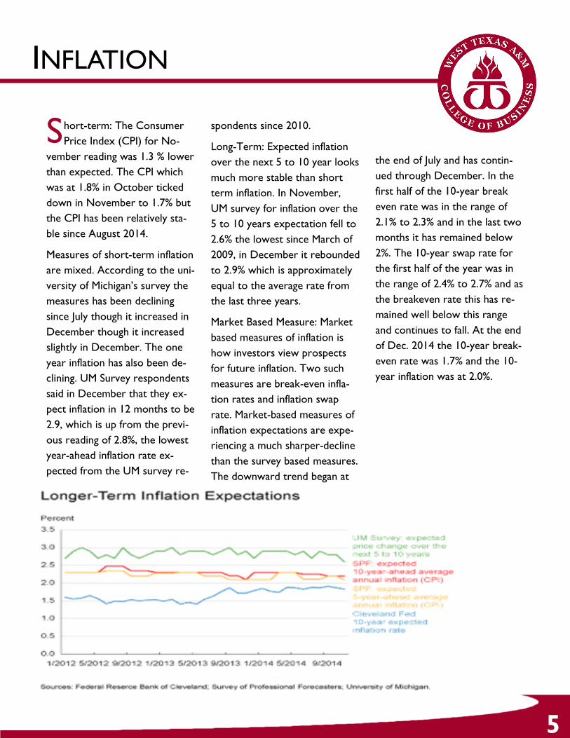
the end of July and has contin-

ued through December. In the

first half of the 10-year break

even rate was in the range of

2.1% to 2.3% and in the last two

months it has remained below

2%. The 10-year swap rate for

the first half of the year was in

the range of 2.4% to 2.7% and as

the breakeven rate this has re-

mained well below this range

and continues to fall. At the end

of Dec. 2014 the 10-year break-

even rate was 1.7% and the 10-

year inflation was at 2.0%.

S hort-term: The Consumer

Price Index (CPI) for No-

vember reading was 1.3 % lower

than expected. The CPI which

was at 1.8% in October ticked

down in November to 1.7% but

the CPI has been relatively sta-

ble since August 2014.

Measures of short-term inflation

are mixed. According to the uni-

versity of Michigan’s survey the

measures has been declining

since July though it increased in

December though it increased

slightly in December. The one

year inflation has also been de-

clining. UM Survey respondents

said in December that they ex-

pect inflation in 12 months to be

2.9, which is up from the previ-

ous reading of 2.8%, the lowest

year-ahead inflation rate ex-

pected from the UM survey re-

spondents since 2010.

Long-Term: Expected inflation

over the next 5 to 10 year looks

much more stable than short

term inflation. In November,

UM survey for inflation over the

5 to 10 years expectation fell to

2.6% the lowest since March of

2009, in December it rebounded

to 2.9% which is approximately

equal to the average rate from

the last three years.

Market Based Measure: Market

based measures of inflation is

how investors view prospects

for future inflation. Two such

measures are break-even infla-

tion rates and inflation swap

rate. Market-based measures of

inflation expectations are expe-

riencing a much sharper-decline

than the survey based measures.

The downward trend began at

DEMOGRAPHICS

6

boomers do not want to go to a nurs-

ing home. Most of retirees want to still

live at home, and have medical services

come to them. This style of medical

care is becoming increasingly popular

and is expected to grow.

On top of the increase in people near-

ing retirement, the life expectancy is

increasing. In 2001 the life expectancy

was 76.5 and now in 2014 is 78.5.

There will not only be an increase in

people demanding healthcare but also

an increase in the time the person will

need the healthcare. Health care com-

panies will have to prepare for more

people and expect the person to live

longer. With both of the factors in-

creasing the demand for health care

services the growth for the healthcare

industry in potentially very strong.

Also with the aging demographics,

there is an increase in demand for lei-

sure activities. With many of the baby

boomers nearing retirement, a majori-

ty of the population will begin to have

more time. A survey conducted by Sta-

tista revealed that many of the baby

boomers what to spend more time do-

ing activities they did growing up.

Reading books, playing in the park, and

many other leisure activities popular in

the 1970s and 1980s are predicted to

grow in the coming years as well.

D emographics play a critical

part of the macroeco-

nomic analysis. The main con-

cern in the United States in

terms of demographics is the

baby boomer generation. When

World War II ended so did the

depression and the economy

was booming. With the econo-

my doing well families began

having a big number a babies.

This big generation has been

moving through the different life

stages at the same time and the

economy has catering to the

needs of the baby boomer gen-

eration. Now the baby boomers

are starting to reach the age of

retirement with the oldest being

the age of 69. With the baby

boomer generation approaching

retirement comes many new

demands for products and ser-

vices. IBIS World explains that

the baby boomers are the larg-

est consumer of healthcare in

the United States, and will con-

tinue to demand a growing num-

ber of in home care services. In

five years there will be 54.2 mil-

lion people 65 or older in the

United States, which will in-

crease the demand for

healthcare products and services

that serve the elderly.

Healthcare firms are already

starting to see demands from

the aging demographics. The

average medical expenses in-

curred by people 65 and over

are just under $10,000 a year.

That is more than $3,000 more

a year than people who are 45

to 64. Older people need more

medical care, and with the baby

boomer generation approaching

retirement the demand is going

to grow dramatically. The types

of services that will see the

most growth are companies that

tend to cater to in-home

healthcare. Many of the baby

85+

80-84

75-79

70-74

65-69

60-64

55-59

50-54

45-49

40-44

35-39

30-34

25-29

20-24

15-19

10-14

5-9

0-4

EXCHANGE RATES

7

A strong economy has a

strong currency. The US/

Euro rate is $1.13. Japan/US rate

is 118.08. Mexico/US is $14.78.

China/US rate $6.299. Oil prices

being at a low price means that

the strength of the U.S dollar is

strong. Oil and the exchange

rate have a high correlation

weighted between each other.

When the oil prices are down,

the U.S. dollar becomes strong-

er. On the other hand with oil

prices rising, this will make the

dollar weaker. The U.S. dollar is

stronger against the other cur-

rencies. The graph above shows

the strength of the dollar to the

euro. Since the euro is at its

lowest in several years, many

American’s are taking advantage

of traveling to Europe at low

prices and saving money on va-

cations or trips.

When the economy is facing pe-

riods of high economic turbu-

lences, the economy can expect

to see higher levels of volatility

occurring. Slower growth and

economic situations abroad are

causing other countries difficul-

ties in trading. Exporters to the

U.S. are seeing growth while

U.S. exporters are experiencing

sluggish revenue.

Source: St. Louis Fed FRED Database

U.S. INCOME DISTRIBUTION

8

of income inequality, it is better to

know what includes in household

income. Household income usually

includes labor income, which is

consisted of wages, salaries and

other work-related compensation,

and capital income, which includes

interest, dividends and other in-

vestment returns. During the last

three decades, labor’s share of to-

tal income has decreased in favor

of capital income. According to

Bureau of Economic Analysis, Bu-

reau of Labor Statistics, and CBO,

there were a significant drop of 3

to 8 percentage points in labor’s

share of income since the early

1980s and the trend would contin-

ue accelerating until recently. The

decline in labor income share of

total income would negatively af-

fect the income inequality. The dis-

tribution of labor income is more

even across U.S household than

that of capital income since a dis-

proportionately huge share of capi-

tal income accrues to the top in-

come households. As a result, the

total income becomes less evenly

distributed and more concentrated

at the top, which create the larger

income inequality. In fact, with eve-

ry percentage point decline in the

labor share of total income, the

Gini index rises by about 0.15 to

0.33 percentage (Congressional

Budget Office).

T he distribution of household

income in the U.S has been

more unequal during the post-2008

economic recovery. The income

distribution in the U.S. is highly

accumulated toward the top, with

the top 10% earning more than half

of country’s total income, and the

top 1% of household received

22.46 percent of all pre-tax income

in 2012. This is based on the differ-

ence in experienced growth of in-

come among different quintiles of

household. According to the Bu-

reau of Labor Statistic’s Consumer

Expenditure Survey, there were an

increase in nominal income of

about $7,100 for the highest in-

come quintile in the U.S, while the

lowest income quintile witnessed a

decline of approximately $360

from 2007 to 2012. This results in

more than 80 percent of the in-

crease in household income ac-

counted by the top 20 percent of

earners between 2008 and 2012.

Therefore, the share of income

earned by the top-income house-

hold went up sharply when the

share accounted by the bottom-

income household reduced.

The other indicators of income

inequality which should be closely

watched is the Gini index. The Gini

index, ranging between 0 and 1 as

the distribution of income be-

comes more dispersed, is equal to

half the relative mean income dif-

ference. The Gini index indicates

the increase in income inequality

during the entire period from 1967

to 2012. Using the Census Bureau

data, the Gini index increased from

0.40 in 1967 to 0.48 in 2011, mean-

ing that the difference in income

between household was 80 per-

cent on average in 1967, while the

figure is 96 percent in 2011.

In order to understand the causes

EXPORTS & IMPORTS

9

volume of trade is expected to

grow to $6.15 trillion by 2020,

at an annualized rate of 4.95%.

Exports are expected to grow at

a compound rate of 4.89% to

$2.75 trillion by 2020, and im-

ports are expected to grow at a

compound rate of 5% to $3.4

trillion. As a result, the trade

deficit is expected to rise to

$650 billion by 2020, compared

with a trade deficit of $505 bil-

lion in 2014.

Exports are currently influenced

by the bad economy in Europe

and the revisions of growth ex-

pectations from China. Coming

along with that the current

strong value of the dollar lowers

the export volume. Policies of

the European Central Bank and

the Bank of Japan have caused

the dollar to strengthen in the

past months and could be a rea-

son for the further boosting of

the dollar value. This would indi-

cate that imports become

cheaper and exports become

more expensive what contrib-

utes to a higher trade deficit. It

is also unlikely that the reported

2.6% gain in fourth-quarter GDP

of 2014 will be revised higher

due to the increase trade deficit.

T he largest trading partners

of the U.S. are the Europe-

an Union, Canada, China, Mexi-

co, and Japan. These countries

account for about two-thirds of

U.S. merchandise trade. Cana-

da’s and Mexico’s high trading

volumes are consequences of

the North American Free Trade

Agreement (NAFTA). The total

value of trade in goods and ser-

vices is sensitive to factors in-

cluding exchange rates, global

economic conditions, income,

and domestic consumer confi-

dence.

Historically, since the 1970s the

United States had a negative bal-

ance of trade. In 2014 the goods

and services deficit amounted to

$505 billion. The deficit in-

creased by about $28.7 billion

compared to 2013, where the

balance of trade was a negative

$476.4 billion. As a percentage

of the U.S. GDP, the deficit in-

creased slightly from 2.8 percent

in 2013 to 2.9 percent in 2014.

In the last years, the U.S. rec-

orded the biggest trade deficits

with China, Japan, Germany and

Mexico. The biggest trade sur-

pluses were recorded with

Hong Kong, Netherlands, Unit-

ed Arab Emirates and Australia.

The graph shows the monthly

trade balance in the last five

years. The $46.6 billion deficit in

December of 2014 was the wid-

est deficit since November

2012. This increase can be partly

attributed to the 31.7% increase

in the imports of crude oil.

Many domestic firms were try-

ing to take advantage of the

cheap oil.

According to IBIS World the

Source: St. Louis Fed FRED Database

FED POLICY & INTEREST RATES

10

Last September, the FOMC is-

sued its statement on Policy

Normalization Principles and

Plans. This statement provides

information about the commit-

tees likely approach to raising

short-term interest rates and

reducing the Federal Reserve's

securities holdings. The com-

mittee intends to reduce its se-

curities holdings in a gradual and

predictable manner primarily by

ceasing to reinvest repayments

of principle from securities held

by the Federal Reserve.

The FOMC’s assessment that it

can be patient in beginning to

normalize policy means that the

committee considers it unlikely

that economic conditions will

warrant an increase in the target

range for the federal funds rate

for at least the next couple of

FOMC meetings.

A s of February 24, 2015 in

Federal Reserve Chair Ja-

net Yellen’s semi-annual report

to Congress the Fed remains

committed to policies that pro-

mote maximum employment

and price stability. The FOMC

judges that a high degree of poli-

cy accommodation remains ap-

propriate to foster further im-

provement in labor market con-

ditions and to promote a return

of inflation toward 2% over the

medium term.

Chairman Yellen stated that

while the drop in oil prices will

have negative effects on energy

producers and will probably re-

sult in job losses in this sector,

causing hardship for affected

workers and their families, it will

likely be a significant overall plus

for our economy. This boost

will arise from US households

having the ability to increase

their spending on other goods

and services as they spend less

on gasoline.

Economic activity may be the

response to policy stimulus now

being provided by foreign cen-

tral banks more strongly than

we currently anticipate, and the

recent decline in the world oil

prices could boost overall global

economic growth more than

expected.

At the time of the February 24th

report, assets held on the Fed’s

balance sheet totaled nearly

$4.5 trillion compared to $995 million in September of 2008.

The target Fed Funds rate is

currently .25% compared to 2%

in 2008. The 10 year treasury’s

current yield is 2.05% compared

to 3.75% pre-crisis.

Mortgage rates have remained

low with the 30 year fixed rate

at 4% and the 15 year fixed

mortgage rate at just above 3%.

0.0

0.5

1.0

1.5

2.0

2.5

3.0

3.5

4.0

4.5

2003 2004 2005 2006 2007 2008 2009 2010 2011 2012 2013

Tri

llio

ns

of

$

Balancing Act

The Federal Reserve board is widely expected to end

the latest in a series of bond-buying programs that

swelled the bank’s balance sheet to unprecedented

size.

Assets on the Federal Reserve

balance sheet, in trillions

Mortgage-Backed Securities

Treasuries

Other Assets

Source: St. Louis Fed FRED Database

GOVERNMENT DEBT & DEFICIT

A government's budget balance

is the difference in govern-

ment revenues (primarily

from taxes) and spending. If spend-

ing is greater than revenue, there is

a deficit. If revenue is greater than

spending, there is a surplus. Deficit

is the added debt in the current

period (month, quarter, and year).

Government debt is the stock of

outstanding IOUs issued by the

government at any time in the past

and not yet repaid. Whenever the

governments borrow money from

the public, they issue debt. Out-

standing debt is cumulated net bor-

rowing that the government has

done over time. As the national

debt grows, that means consequen-

tially private investments are going

to shrink which means lowering

future growth and future wages. At

the moment, United States national

debt is well over 18 trillion dollars

which is the highest national debt in

the world. Simple math reveals that

each citizen of the US has almost

$57,000 share in the national debt

and that U.S. government has been

increasing the debt by $2.4 billion

per day for the last three years.

Because the U.S. is one of the most

powerful economies of the world,

its debt negatively affects other

economies around the world that

are relying on the U.S.’ output and

growth. Figure 1.1 shows the most

indebted nations in the world when

it comes to debt-to-GDP ratio.

There are two different deficits;

cyclical deficit and structural deficit.

In the case of cyclical deficit there

is high level of unemployment at

the lowest level of the business

cycle which means that tax reve-

nues are low and expenditures are

high leading to a budget deficit. This

kind of deficit is a stabilizer in the

economy as it can have stimulating

effects on the economy by increas-

ing demand, spending and investing.

Structural deficit remains through-

out the whole business cycle due

to general level of government

spending exceeding prevailing tax

levels. It happens when the econo-

my is at full employment and is

producing at full output levels. The

11

only way this gap can be closed is

to increase revenues or cut spend-

ing. In structural deficit, govern-

ment must issue more bonds which

reduces the price of bonds and in-

creases interest rates and that

means reduction in private invest-

ment demand (crowding out).

Higher interest rates also increase

demand for the dollars and reduces

its supply in the foreign exchange

market which raises the exchange

rate and that leads to reduced net

exports. High structural debt has

negative consequences for the

economy.

7 Highest Debt-to-GDP Ratios

Source: WHERE DID THIS COME FROM?!?!

OIL PRICES & GDP GROWTH

12

and financial markets such as the

S&P500, USD exchange rate,

and U.S. Treasury bonds on a

daily basis. Typically, the S&P500

and oil prices move together,

while oil prices have conversely

moved in the opposite direction

of Treasury bonds, and the dol-

lar’s exchange rate. The market

responds to risk/return levels

similarly between stocks and oil,

so as can be expected, when

there is significant risk in the

market, less money flows into

stocks and oil, while bonds ex-

perience an inflow.

G lobal oil prices impact do-

mestic growth, and during

2014 into 2015, oil prices

dropped nearly 50%. Typically,

when oil prices are low, the U.S.

economy is able to take ad-

vantage of this and enjoy signifi-

cant growth in production lev-

els, especially in the petrochemi-

cal and new cars industries.

However, recently, the demand

has been mostly unresponsive to

the lower prices. This is due pri-

marily to increased production

in North America, unsubstantial

global demand growth, & sus-

tained high levels of production

by OPEC. Since the U.S. has re-

strictions on exporting oil, pro-

ducers lack the ability to seek

out the highest price available

for their production, placing ad-

ditional downward pressure on

U.S. prices. Also, prices may face

further downward pressure due

to the likely increase in produc-

tion by Iran if nuclear sanctions

against them are lifted.

Outlook and Implications

High oil price volatility will likely

persist through the next five

years. Demand is catching back

up to the supply levels, and pric-

es are expected to gradually re-

bound, and trend slightly up-

ward through 2020. As oil is a

major input for many industries

products, and global production

levels are expected to be more

than sufficient, there will contin-

ue to be an increasing intensity

of competition on the national

and global levels. The industry

in the U.S. will continue to

move through a phase of con-

solidation, so shale producing,

plus other E&P’s are expected

to remain at discount levels. In-

dustrial manufacturers will bene-

fit from the lower prices, and

growth in the petro industry

should also continue to gain at-

traction.

The chart below displays the co-

movements in oil futures prices

Correlations (+ or - ) Between Daily Returns on Crude Oil Futures and Financial Investments

WTI Crude Oil Price Peak

Source: U.S. Energy Information Administration

BUY/SELL DECISIONS

13

The portfolio managers started with over 150 stocks. Throughout the

spring 2015 semester, the students analyzed the stocks and decided on

buying the following five stocks.

LITHIA MOTORS (LAD)

Diversified Business

Industry Leader

Strong Ratios Versus Industry

Control of Every Sales Stage

Low P/E and Debt/Equity

High Revenue Growth

Risk: Volatile Oil Prices

Expected Future Price: $150

MICRON TECHNOLOGY (MU)

Strong R&D

Growth Opportunities from Solid

State Drives

Industry Leader in DRAM &

NAND Manufacturing

Positive Outlook from

Smartphone and Tablet Market

Risk: Cyclical Industry

Expected Future Price: $50

SOUTHWESTERN ENERGY CO. (SWN)

Growing Revenues

Excellent Management

Involved in Low Cost Plays

Risk: Increased Debt Levels

Expected Future Price: $45

AON PLC. (AON)

Growing Sales

Diversified Client Base

Global Presence

Strong Acquisitions

Risk: Large pension obligation

Dividend Yield: 1.2%

Expected Future Price: $145

SELLS: THE FOLLOWING STOCKS REACHED

VALUATION AND WERE SOLD

Altera

CA

EMC

Ford

Wendy’s

Xcel

DOMTAR CORPORATION (UFS)

Wide Range of Recognized Products

High Dividend Growth

Steady EPS Growth

Extensive Distribution Network

Risk: Short-term Price Volatility

Dividend Yield: 3.7%

Expected Future Price: $60

PORTFOLIO MANAGERS

14

KARINA ACEVEDO

Karina is a senior finance major from Texhoma, OK. She is currently a finance intern at Street Toyota. She

enjoys lifting weights and watching movies in her spare time. Karina competed in the West Texas Strong

Man Competition and placed in the top three.

EDDIE BOYD

Eddie is a senior finance major from Amarillo, TX. Eddie works in a family financial services business and

enjoys non-profit board work. Eddie and his wife Lisa have five children ages 21 through 25.

CHELCI CASTILLO

Chelci is a senior finance and accounting major from Amarillo, TX. She currently works as a part time teller

at Wells Fargo Bank in Amarillo. In her spare time she enjoys playing volleyball, being outdoors, and spend-

ing time with family and friends.

HUNTER HAM

Hunter Ham is a senior MSFE student from Houston, Texas, who is only two electives away from graduat-

ing. He was induced into Beta Gamma Sigma in October of 2013 here at WT, where he completed his un-

dergrad in August of 2014. Hunter has found Canyon a wonderful place to remain focused on only the task

at hand, since he loves to fish and surf, and not even “SIRI” knows where the closest beach is from Can-

yon. His professional passion is geared toward corporate strategy within the oil and gas industry, either up-

stream, or midstream.

KLEMEN JEREB

Klemen is a senior finance major from Ljubljana, Slovenia. Before coming to WTAMU, he was a member of a

national championship soccer team. He is also a member of Sigma Nu fraternity, and honor societies such as

Order of Omega and IFC. In his spare time he likes to play soccer and enjoys the outdoors.

HONGYU LI

Hongyu is an MSFE student from Tianjin, China. He will be graduating in December of 2015.

PORTFOLIO MANAGERS

15

FABIAN MULLER

Fabian is a senior finance major from Amtzell, Germany. He is a student-athlete that runs Track & Field for

WTAMU. In 2011 he was also a member of the Junior National Team of Germany for Track & Field . His

hobbies include skiing and wind-surfing.

PHUC NGUYEN

Phuc is a graduate student from Vietnam and is in the MSFE program at WTAMU. He is a member of this

years CFA Research Challenge Team, a member of Enactus, and the National Society of Leadership and Suc-

cess. In his spare time, he likes to play soccer or exercise.

ETHAN PETERSON

Ethan is a Senior Finance major from Texico, New Mexico. He will graduate in August and plans to enter

the MSFE program. He is also a member of the West Texas A&M golf team and plans to finish out his last

year of eligibility while going through the MSFE program.

SAHIL PRASLA

Sahil is senior Health Science major with a minor in Finance. He is planning to attend WT to pursue he Mas-

ters in Finance and Economics. He will be graduating from the LEAD WT program, he is also a President’s

Ambassador and served on various student affair’s committee. In his spare time he likes to play cricket.

VITALIY SKORODZIYEVSKIY

Vitaliy is a graduate student, pursuing the MSFE degree at WTAMU. He graduated with a bachelor’s degree

from WT in International Business. He is a part of the university’s CFA Research Challenge team. Vitaliy was

a part of Honor’s Programs, LEAD WT, and COB’s Student Advisory Board. In his spare time he likes to

play volleyball.

TYLER J. YOUNG

Tyler is a Canyon native and a graduate student at WTAMU majoring in Finance and Economics. He is also a

member of the university’s CFA Research Challenge team, Omicron Delta Epsilon honor society, and Beta

Gamma Sigma honor society. Tyler enjoys skiing and watching movies in his down time.

SCHOLARSHIP WINNERS

16

For the 2015-16 academic year, the Student-Managed Investment Fund awarded

$15,000 in scholarships. Scholarships ranged from $1,000 to $2,000 in value. Since

2001, the SMIF has awarded $132,500 in scholarships.

Paul Alongo, a senior Marketing major from Canyon, Texas

Adriana Gallegos, an MBA student from Amarillo, Texas

Alexander Korn, an MBA student from Kehl, Germany

Michelle McFadden, a freshman General Business major from Amarillo, Texas

Baptiste Moreu, an MSFE student from Auray, France;

Fabian Mueller, an MSFE student from Amtzell, Germany

Nicholas Shelton, an MSFE student from Amarillo, Texas

Phuc Nguyen, an MPA student from Vietnam

Ethan Peterson, an MSFE student from Canyon, Texas;

Doores Athletic Scholarships

Jamie Boyd, a junior Marketing major from Abilene, Texas; baseball

Michaela Neuhaus, a senior International Business major from Lone Tree, Colorado;

basketball

Christian Suthers, a junior General Business major from Preston, England, United Kingdom;

soccer

Jordan Evans, a sophomore General Business major from Houston, Texas; basketball

Eric Mosley, a sophomore General Business major from Gilbert, Arizona; basketball

STUDENT-MANAGED

INVESTMENT FUND

ANNUAL REPORT

2015