structuresoftheoceaniclithosphere-asthenosphereboundary ... · mineral-physics modeling and...

Article

Volume 14, Number 4

17 April 2013

doi:10.1002/ggge.20086

ISSN: 1525-2027

Structures of the oceanic lithosphere-asthenosphere boundary:Mineral-physics modeling and seismological signatures

T. M. Olugboji, S. Karato, and J. ParkDepartment of Geology and Geophysics, Yale University, P.O. Box 208109, New Haven, Connecticut,06520-8109, USA ([email protected])

[1] We explore possible models for the seismological signature of the oceanic lithosphere-asthenosphereboundary (LAB) using the latest mineral-physics observations. The key features that need to be explainedby any viable model include (1) a sharp (<20 km width) and a large (5–10%) velocity drop, (2) LAB depthat ~70 km in the old oceanic upper mantle, and (3) an age-dependent LAB depth in the young oceanic uppermantle. We examine the plausibility of both partial melt and sub-solidus models. Because many of the LABobservations in the old oceanic regions are located in areas where temperature is ~1000–1200�K, significantpartial melting is difficult. We examine a layered model and a melt-accumulation model (at the LAB) andshow that both models are difficult to reconcile with seismological observations. A sub-solidus modelassuming absorption-band (AB) physical dispersion is inconsistent with the large velocity drop at theLAB. We explore a new sub-solidus model, originally proposed by Karato [2012], that depends ongrain-boundary sliding. In contrast to the previous model where only the AB behavior was assumed, thenew model predicts an age-dependent LAB structure including the age-dependent LAB depth and itssharpness. Strategies to test these models are presented.

Components: 10,500 words, 18 figures, 3 tables.

Keywords: lithosphere-asthenosphere boundary; grain-boundary sliding; subsolidus; anelasticity; partialmelting.

Index Terms: 7218 Seismology: Lithosphere (1236); 8120 Tectonophysics: Dynamics of lithosphere andmantle: general (1213); 3909 Mineral physics: Elasticity and anelasticity.

Received 14 September 2012; Accepted 6 February 2013; Published 17 April 2013.

Olugboji T. M., S. Karato, and J. Park (2013), Structures of the oceanic lithosphere-asthenosphere boundary: Mineral-physics modeling and seismological signatures, Geochem. Geophys. Geosyst., 14, 880–901, doi:10.1002/ggge.20086.

1. Introduction

[2] The lithosphere and the asthenosphere aredefined through their mechanical properties. Thephysical reasons for a strong lithosphere over a weakasthenosphere are important, influencing how platetectonics operates on Earth. Mechanical definitionsbased on seismicity, plate bending (flexure), and

gravity anomalies have yielded “lithosphere” withthicknesses from 20 km to 200 km in the sameregions [McKenzie, 1967; Nakada and Lambeck,1989; Peltier, 1984; Karato, 2008]. For example,using post-glacial-rebound observations, Peltier[1984] inferred ~200 km continental lithospherewhereas Nakada and Lambeck [1989] inferred~50-km continental lithosphere, making it difficult

©2013. American Geophysical Union. All Rights Reserved. 880

to investigate causal influences on lithosphere-asthenosphere boundary (LAB) depth.

[3] In addition to the mechanical constraints onLAB, other proxies have defined the LAB depth,e.g., petrology, temperature, electrical conductivity,and seismic wavespeeds [Eaton et al. 2009]. Thesedifferent proxies have their advantages, but in thispaper, we argue that the seismic wavespeeds bestdefine the LAB [e.g., Jones et al., 2010; Behnet al., 2009].

[4] Puzzling results in both the oceanic and conti-nental regions suggest that existing models for the“seismological” LAB need to be revisited. In theoceans, Kawakatsu et al. [2009] and Kumar andKawakatsu [2011] observed a shallow (~60 km)and large velocity drop (~7%), in some old(~100–130 Ma) oceans. In the old continents,strong mid-lithospheric discontinuities (MLD) areobserved at the depth of ~100–150 km, but nostrong signals at depths ~200 km, where we wouldexpect the LAB [Abt et al., 2010; Ford et al., 2010;Rychert and Shearer, 2009; Rychert et al., 2007;Thybo, 1997; 2006]. Karato [2012] argues thatpartial melting, a popular model for the LAB, isnot expected at these depths in these regions,nor can the inferred large velocity drop beexplained readily by a standard absorption-band(AB) anelastic model.

[5] In this paper, we review important shortcomingsto the previous partial melt and sub-solidus modelsfor the oceanic LAB. Then, we develop a newsub-solidus model, based on grain-boundary sliding,originally proposed by Karato [2012]. Our analysisextends the previous study via a new statisticalanalysis of experimental data to provide robustconstraints on key parameters, allowing a moredetailed discussion of their uncertainties.We introducea new parameterization for grain-boundary-slidingattenuation and velocity reduction that capturesbetter the features of theoretical models, whilebeing functionally simple. We also explore a varietyof published thermal models for the oceanic sea floor[Davies, 1988; McKenzie et al., 2005; Parsons andSclater, 1977; Stein and Stein, 1992] to characterizethe sensitivity of our results to uncertainties inthermal models, as well as exploring the agedependence of oceanic LAB structures. Modelsfor the seismological observations of continentalLAB will be discussed in a separate paper wherewe will discuss the origin and significance ofMLD and the reasons for weak seismic signalsfrom the supposed LAB using the mineral-physicsmodels similar to those developed here.

2. Models of the Oceanic LAB

2.1. Difficulties with the Partial-meltModels

[6] A popular model to explain a sharp, large velocitydrop at the LAB is the onset of partial melting[Anderson and Sammis, 1970; Anderson andSpetzler, 1970; Lambert and Wyllie, 1970]. Inorder for a partial-melt model of LAB to be valid,two conditions must be met. First, the temperatureat the LAB must exceed the solidus. Second, themelt fraction below the LAB must be large enoughto cause a large velocity reduction. To reducevelocity by 5–10% in the shallow upper mantle,one will need 3–6% melt fraction [Takei, 2002].We evaluate below various partial-melt modelswith special attention to these two points.

2.1.1. Thermal Structures of theLithosphere-asthenosphere

[7] In all partial-melt models, it is essential that theLAB temperature corresponds to the depth at whichgeotherm intersects the solidus. The simplest modelthat prescribes the temperature distribution in theoceanic upper mantle is the halfspace-cooling model[Davis and Lister, 1974; Turcotte and Schubert,2002]. In this model, only one free parameter, thedifference ΔT between the surface temperature andthe potential temperature, prescribes completely thetemperature distribution. As the plate moves awayfrom the ridge, it cools conductively with timefollowing the

ffiffit

page dependence. The typical value

for ΔT is 1350�K, which is within the bounds ofpetrological constraints on the ambient mantlepotential temperature, Tp ~1550–1600�K [McKenzieand Bickle, 1988]. The model predicts ~1030�K at 60km in the 120 my old oceanic upper mantle. Weconclude that the observed shallow depths of theLAB in the old oceanic upper mantle are difficult toreconcile with a partial-melt model with thesegeothermal structures.

[8] In the plate model, one assumes that the temper-ature at a certain depth is fixed, e.g., by the onset ofsmall-scale convection [McKenzie et al., 2005;McKenzie, 1967]. Consequently, plate models ingeneral predict higher temperatures in the oldoceanic upper mantle. The temperature at theLAB (e.g., 60 km in 120 Ma mantle) for platemodels depends on the choice of plate thicknessand the base temperature. McKenzie et al. [2005]provided one such plate model with a potentialtemperature of 1588�K (constrained by the crustal

GeochemistryGeophysicsGeosystemsG3G3 OLUGBOJI ET AL.: STRUCTURES OF THE OCEANIC LAB 10.1002/ggge.20086

881

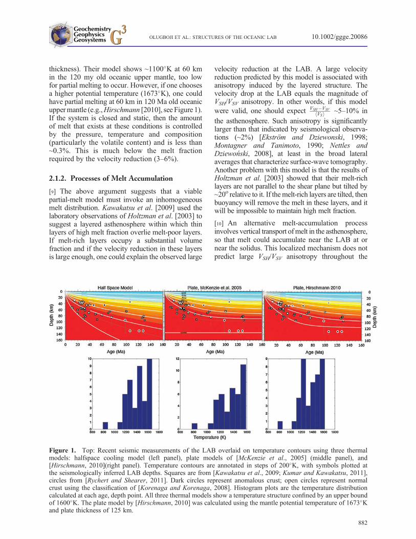
thickness). Their model shows ~1100�K at 60 kmin the 120 my old oceanic upper mantle, too lowfor partial melting to occur. However, if one choosesa higher potential temperature (1673�K), one couldhave partial melting at 60 km in 120 Ma old oceanicuppermantle (e.g.,Hirschmann [2010], see Figure 1).If the system is closed and static, then the amountof melt that exists at these conditions is controlledby the pressure, temperature and composition(particularly the volatile content) and is less than~0.3%. This is much below the melt fractionrequired by the velocity reduction (3–6%).

2.1.2. Processes of Melt Accumulation

[9] The above argument suggests that a viablepartial-melt model must invoke an inhomogeneousmelt distribution. Kawakatsu et al. [2009] used thelaboratory observations of Holtzman et al. [2003] tosuggest a layered asthenosphere within which thinlayers of high melt fraction overlie melt-poor layers.If melt-rich layers occupy a substantial volumefraction and if the velocity reduction in these layersis large enough, one could explain the observed large

velocity reduction at the LAB. A large velocityreduction predicted by this model is associated withanisotropy induced by the layered structure. Thevelocity drop at the LAB equals the magnitude ofVSH/VSV anisotropy. In other words, if this modelwere valid, one should expect VSH�VSV

VSh i ~5–10% in

the asthenosphere. Such anisotropy is significantlylarger than that indicated by seismological observa-tions (~2%) [Ekström and Dziewonski, 1998;Montagner and Tanimoto, 1990; Nettles andDziewoński, 2008], at least in the broad lateralaverages that characterize surface-wave tomography.Another problem with this model is that the results ofHoltzman et al. [2003] showed that their melt-richlayers are not parallel to the shear plane but tilted by~20o relative to it. If themelt-rich layers are tilted, thenbuoyancy will remove the melt in these layers, and itwill be impossible to maintain high melt fraction.

[10] An alternative melt-accumulation processinvolves vertical transport ofmelt in the asthenosphere,so that melt could accumulate near the LAB at ornear the solidus. This localized mechanism does notpredict large VSH/VSV anisotropy throughout the

Figure 1. Top: Recent seismic measurements of the LAB overlaid on temperature contours using three thermalmodels: halfspace cooling model (left panel), plate models of [McKenzie et al., 2005] (middle panel), and[Hirschmann, 2010](right panel). Temperature contours are annotated in steps of 200�K, with symbols plotted atthe seismologically inferred LAB depths. Squares are from [Kawakatsu et al., 2009; Kumar and Kawakatsu, 2011],circles from [Rychert and Shearer, 2011]. Dark circles represent anomalous crust; open circles represent normalcrust using the classification of [Korenaga and Korenaga, 2008]. Histogram plots are the temperature distributioncalculated at each age, depth point. All three thermal models show a temperature structure confined by an upper boundof 1600�K. The plate model by [Hirschmann, 2010] was calculated using the mantle potential temperature of 1673�Kand plate thickness of 125 km.


882

asthenosphere. In addition, there must be a process tomaintain a large melt fraction (3–6%) near the LABto a layer that is thick enough to produce a strongseismic signal. The structure of such a region(i.e., the melt fraction and its variation with depth)is controlled by the competition of gravity-inducedcompaction, melt accumulation, melt generation,and transport. Therefore, one needs to have a specificcombination of solid-matrix viscosity, permeability,etc. to maintain a layer that explains the seismologicalobservations. None of these parameters areconstrained well, and therefore we conclude thatthis model remains speculative.

2.1.3. Seismological Consequences of anAccumulated Melt Model for the LAB

[11] As a further test, we compute Ps and Spreceiver functions using synthetic seismograms forvelocity variations implied by a melt-accumulationmodel (Figure 2). To detect a melt-rich layer inthe RF signals, several conditions must be met:(1) the wavelength of the seismic signal must becomparable to the layer thickness, or smaller, and(2) the velocity (impedance) jump must be strongenough to make the signal visible [e.g., Leahy,2009; Leahy and Park, 2005]. With sensitivity

Figure 2. Synthetic receiver functions computed using a model given in (D), which represents a low-velocity layer(LVL) embedded at a depth of 70 km, as would be required by a melt layer with ~7% reduction in shear wave velocity.The lower panel describes schematically the conversions for an incident P phase (C) or an incident S phase (E). Thesynthetic seismograms for the P and S phases show conversions on the vertical (Z, in red) and radial (R, in blue) com-ponents. Receiver functions are then computed from this synthetic data using the method of [Park and Levin, 2000].The Ps receiver function shows a closely spaced double polarity conversion following the initial pulse at time zero.The Psd1 phase, which is generated from the top of the melt layer, is followed by the Psd2 phase, generated fromthe bottom of the layer. In the case of the Sp receiver functions, the sequence is reversed (B). The double polarity sig-nals arrive before the initial pulse with the Spd2 phase arriving before the Spd1 phase (B). The double polarity signal isindicative of a low-velocity layer. In our computation of the receiver functions, we rotate the synthetic seismogramsfrom the ZRT coordinates into the LQT coordinates to minimize the energy at zero time, which enables a better res-olution of the converted phases. Amplitudes in the first 4 s for the radial and vertical component of the synthetic seis-mogram are scaled by 7% for display purposes. The Ps and Sp receiver functions are computed at a cut-off frequencyof 1Hz and a melt layer thickness of 20 km.


883

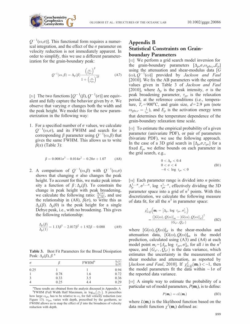
tests, we demonstrate the limitations of receiverfunctions for detecting a melt-rich (low-velocity)layer of variable thickness (Figure 3). Based onthe receiver-function technique of Park and Levin[2000], (see also Leahy et al. [2012]), a cut-offfrequency of 1Hz would resolve a melt layer thick-ness >5 km. In a more general case, the peak-to-peak amplitude depends on the magnitude ofthe velocity drop: the larger the magnitude of thevelocity drop, the larger the peak-to-peak amplitude(Figure 4). In real data, high noise levels will makelow amplitude RF signals difficult to detect.

[12] Another aspect of a melt-accumulation model isa possible signal from the bottom boundary. If bothtop and bottom boundaries are sharp (Figure 2), therewill be a double-polarity signal: a negative phase(Psd1 and Spd2) generated from conversions at

the top of the melt layer (the inferred LAB in mostseismic studies), followed by a positive phase(Psd2 and Spd1), generated from conversions at thebottom of the low-velocity layer (LVL).

[13] However, the bottom boundary of the melt-accumulation zone could be gradational. Such adiffuse boundary would not produce sharp convertedphases from the lower boundary of the melt-accumulation layer (Figure 5). For sharp velocitygradients (<15 km), the pulse from a bottom boundaryshould be detectable at frequencies >0.3 Hz. Abroader velocity gradient>20 km requires computa-tion of the receiver function in multiple frequencybands to clearly distinguish the pulse. For instance,a gradient width of 40 km at 0.3 Hz is so wide; sucha pulse could be buried in the background noise. Athigher frequencies, however (e.g., 1.5Hz), the pulse

Figure 3. Sensitivity tests for Ps receiver functions through a low-velocity layer with varying thickness. Themagnitude of the velocity drop is 7%. The peak-to-peak amplitude and time separation (A) are measured. For a thicknessof 5 km and 0.3 Hz, the low-velocity layer is hard to detect (A, lower panel). For a thickness of 20 km and 1 Hz, thelayer is easily identified (A, top panel). The cut-off frequency for detection becomes lower with larger thickness.The time separation between the negative and positive polarity, increases as thickness increase (C). The estimate of timeseparation also becomes stable at high frequency, since it is difficult to estimate the timing due to the broadening of thepulse in time.


884

becomes discernable with a 6 s pulse width. Usingmultiple frequency bands, which take advantage ofthe high amplitude at low frequencies, and narrowerpulse width at high frequencies, diffuse boundariescould be detected (Figures 3, 4, and 5).

[14] Current RF studies show only a single convertedpulse, either Sp or Ps, inconsistent with a melt-accumulation model with a sharp bottom boundaryor with a thin melt-rich layer. The typical frequenciesof LAB detection are lower than the cut-off frequencyof 1Hz for detection of a thin melt-rich layer.Re-evaluation of seismic data at higher frequencieswould provide better test of the melt-accumulationmodel, but may be feasible only with Ps receiverfunctions. In comparison, receiver-function studiesof the upper mantle above the 410 km discontinuity[Tauzin et al., 2010] show such a double-lobed polar-ity, consistent with a thick partial-melt layer.

2.2. Difficulties with the AB Version ofSub-solidus Model

[15] Karato and Jung [1998] provided a model toexplain a sharp LAB velocity drop using a sub-solidus model, exploring the role of a sharp change

in water content across ~70 km depth. Theyhypothesized that water enhances anelastic relaxationand hence results in a sharp velocity drop at the LAB.Karato and Jung [1998] assumed a simple model ofanelastic relaxation where velocity reduction isdirectly related to the seismic attenuation Q� 1, viz.,the “AB” model of Anderson and Given [1982] andMinster and Anderson [1981]

dVVo

� �ABM

¼ 1

2cot

pa2

� �Q�1 o; T ;P;Cwð Þ � Q�1 (1)

where o is the frequency, T, is the temperature, andCw is the water content.

[16] In the asthenosphere, Q ~ 80 [Dziewonski andAnderson, 1981]; therefore, it is expected that thevelocity drop will be small (< 1%). This result isnot consistent with recent seismic observables thatshow a 5–7% drop in seismic wave velocities.Assuming the AB model, it will require much lowerQ as pointed out by [Yang et al., 2007]. Since this isnot the case, another mechanism must be requiredthat does not affect Q but reduces seismic wavevelocity in the observed frequency band. Such amechanism has been proposed by Karato [2012]

Figure 4. Sensitivity tests for Ps receiver functions through a low-velocity layer showing how changes in themagnitude of the velocity drop dV/Vo affect the peak-to peak amplitude. The larger the amplitude of the velocity drop,the larger the peak-to-peak amplitude (A and B). The detection of a low-velocity layer is dependent on the thickness ofthe low-velocity layer, and the amplitude of the velocity drop (C): the larger the amplitude, the easier it is to detect.


885

(see also [ Karato, 1977]), in the form of a high-frequency dissipation peak due to grain-boundarysliding, which we discuss next.

3. A Modified Sub-solidus Model

3.1. Introduction

[17] Theoretical studies on the deformation of poly-crystalline material have demonstrated that anelasticrelaxation and long-term creep in these materialsoccur as a successive process of elastically accommo-dated grain-boundary sliding followed by accommo-dation via diffusional mass transport [Ghahremani,1980; Kê, 1947; Morris and Jackson, 2009; Raj andAshby, 1971; Zener, 1941]. These studies also

showed that the magnitude of the modulus reduction(relaxation) caused by the elastically accommodatedgrain-boundary sliding can be as much as ~30%,and hence the influence of such a process on thereduction of seismic wave velocities can besubstantial. However, until recently, this relaxationmechanism has been difficult to observe in experi-mental studies of upper-mantle materials. As aresult, its implication for seismic structure of theLAB has not been explored.

[18] Due to significant improvements in experimentalmethodology and empirical parameterizations, somegroups [Jackson and Faul, 2010; Sundberg andCooper, 2010] have reported observations of thegrain-boundary mechanism in mantle peridotites.The experimental evidence of a high-frequency

Figure 5. Sensitivity tests for Ps receiver functions through a diffuse velocity gradient with varying gradient width (A).The pulse width and the amplitude are measured (B) and depend on the seismic frequency as well as the gradient width.For sharp velocity gradients (<15 km), a distinct pulse with maximum amplitude is resolved at frequencies >0.3Hz(C and D). Diffuse velocity gradients (>20 km) require that the receiver function be computed at multiple frequencybands for clear resolution, since lower frequencies have a broad pulse (B, lower panel) and higher frequencies havelow-amplitudes but a sharper pulse (B, top panel). Combining multiple frequencies and checking persistence across thefrequency band can help resolve the character of a melt layer with a gradient in melt fraction.


886

dissipation peak confirms theoretical studies andshows that the AB model alone is insufficient tocharacterize fully the anelasticity at upper-mantleconditions [e.g., Karato, 2012]. The relevant“seismological” effect of a high-frequency peaksuperimposed on the AB model is a significantreduction in velocity (caused by the modulus relax-ation), as the characteristic frequency of grain-boundary sliding ogbs shifts relative to the seismicfrequency os (see Figure 2 of Karato [2012]). Apossible explanation for a large velocity drop(with a modest Q) at the LAB is for ogbs< os inthe lithosphere, but ogbs> os in the asthenosphere.

[19] In its simplest form, the influence of grain-boundary sliding can be understood using a single-Debye-peakmodelwhere the attenuation and associatedvelocity reduction are given by:

Q�1 oð Þ ¼ Δp

osogbs

� �1þ os

ogbs

� �2 (2)

dVVo

� �GBS

¼ Δp

2

1

1þ osogbs

� �2 (3)

where Δp is the relaxation strength of the Debyepeak, os is the seismic frequency, and ogbs is thecharacteristic frequency of the peak mechanism(grain-boundary sliding). We focus on the followingthree points: (1) the sharpness of the velocity change,(2) the amplitude of the velocity change, and(3) the depth at which a sharp and large velocitychange occurs. According to this model, the depthvariation in seismic wave velocity is caused by thedepth variation of the characteristic frequency ofgrain-boundary sliding (ogbs), in addition to thecontribution from an anharmonic effect. Whenogbs> os, the velocity becomes lower. If ogbs

changes abruptly with depth, one expects asharp velocity change. Such abruptness is plausiblefor a water-based effect because mantle water con-tent could change abruptly due to dehydration[Hirth and Kohlstedt, 1996; Karato and Jung,1998]. If the frequency range covered by a shiftingogbs is entirely within the AB regime, then the var-iation in seismic wave velocity is limited by thevalue of Q. For a typical Q (~80), the amplitudeof velocity change is<1%. When the characteristicfrequency ogbs shifts across the seismic frequen-cies, then the GBS peak has greater influence onseismic velocities.

[20] To explain the relatively sharp and large velocitydrop observed at the LAB, it is critical to constrainthe details of the GBS relaxation (peak frequency,

anelastic relaxation strength, and the sharpness ofthe peak). The temperature dependence of attenuationand velocity reduction comes from the temperaturedependence of characteristic frequencies, oAB andoGBS. Because these characteristic frequencies arethe inverse of characteristic times that are connectedto microscopic “viscosity”,oAB andoGBS also likelydepend on water content as [e.g., Karato, 2003;Karato, 2006; McCarthy et al., 2011], viz.,

o T ;Cwð Þoo To; ;Cwoð Þ ¼

d

do

� ��m Cw

Cwo

� �r

exp � Ep

RTo

ToT

� 1

� ��

expVp

R

P

T� Po

To

� �� (4)

whereTo,Cwo, do, andPo are the reference temperature,water content, grain size, and pressure, respectively;Ep and Vp are the activation energy and the activationvolume; and r andm are nondimensional constants thatdescribe the sensitivity of theogbs to water content andgrain size. In the case of a dry mantle, r=0, the depthvariation in ogbs is solely caused by temperaturevariation (with a small effect of pressure), and ogbs

increases gradually with depth. Therefore, the LABshould be gradual, the width depending on thetemperature gradient. However, for the case of awet mantle, r = 1 or 2, the change in characteristicfrequency can be sharp if water content changesabruptly, which would cause a sharp drop in velocity(see Figure 3 of Karato, [2012]).

3.2. Influence of the Peak Width

[21] The actual GBS relaxation peakmay bemore dif-fuse than the simplest model, due to the distribution ofrelaxation peaks. This influences the sharpness of thevelocity gradient. Therefore, we extend the approach

taken by Karato [2012] by modifying dVVo

� �GBS

to

include the broadness of the high-frequency peakobserved in laboratory measurements [Jackson andFaul, 2010; Sundberg and Cooper, 2010]. The relax-ation time for grain-boundary sliding is

t ¼ �bd

Gud(5)

where �b is the grain-boundary viscosity, d is thegrain size, Gu is the unrelaxed shear modulus, andd is the grain-boundary width. The distribution ofd and �b produces a distribution of relaxation times.In their experimental study of aluminum andmagnesium oxide polycrystalline ceramic aggre-gates, Pezzotti [1999] observes a broadening of theDebye peak, which they attribute to the distribution


887

of grain-boundary types. Also, a theoretical study byLee and Morris [2010] demonstrates that the grain-boundary peak broadens when the viscosity and/orgrain size varies within a bulk specimen.

[22] We apply a semi-empirical approach to param-eterize the broadening of the grain-boundary peak.The physical model employed by Jackson and Faul[2010] incorporates this broadening with a log-normal distribution for the relaxation time arounda dominant peak centered at ogbs:

Dp tð Þ ¼ s�1 2pð Þ�1=2 exp� ln togbs

=s

� �22

( )(6)

[23] This formulation of a relaxation timescaledistribution Dp(t) introduces an extra parameter s,which describes the broadening of the grain peakaround ogbs. The s parameter broadens the attenu-ation function and weakens its peak intensity. Inthis study, we model this same effect by using aLorentzian form for the attenuation function:

Q�1 o;bð Þ ¼ Δp bð Þosogbs

� �b

1þ osogbs

� �2b (7)

where the b parameter, similar to the s parameter,defines the broadening around the peak, and theshrinking of the peak intensity is captured by Δp

(b). This form provides us with a convenient wayto explore plausible b values that are acceptable bythe current experimental data. We describe the trans-formation [s⇒b,Δp(b)] by fitting our functionalform to the physical parameterization reported byJackson and Faul [2010], (Appendix A). This resultsin a modification of equation (3) to give:

dVVo

� �GBS

¼ Δp

2

1

1þ osogbs

� �2b (8)

with this modification, we have a combined equa-tion for relative velocity change parameterized bythe variables: (a, T(z,t),b, r):

dVVo

� �tot

a;T z; tð Þ;b; rð Þ ¼ dVVo

� �ABM

þ dVVo

� �GBS

(9)

where a is the frequency dependence from the ABmodel: Q� 1 ~o� a, T(z,t) is the temperature calcu-lated at depth z, t is age, b is the grain-boundarybroadness parameter, and r is the water-sensitivityexponent. We fix the parameter a=0.3, constrainedby experiments.

[24] Again, it is instructive to note that the velocity

reduction dVVo

� �ABM

associated with the AB model

alone is minimal, ~1%. Therefore, we argue thatthe most promising cause of a velocity reduction

is dVVo

� �GBS

, which is controlled by temperature

and water effects through shifts in the characteristicfrequency (4).

3.3. Experimental Constraints on Grain-boundary Sliding Parameters

[25] Most previous experimental studies were made atwater-poor conditions (except for an exploratory studyby Aizawa et al., [2008]), and, consequently, we lackstrong experimental constraints on the water sensitivityparameter, r. However, as discussed by Karato [2006]andMcCarthy et al. [2011], there is a close connectionbetween the characteristic time of anelastic relaxationand the Maxwell time (characteristic time for plasticdeformation). Maxwell time depends on water contentas tM ¼ 1

oM/ C�r

w with r~1–2 (e.g., Karato [2008]),and we use r=1 and 2 in this study.

[26] We determine the plausible range of sub-solidus parameters that is compatible with theexperimental observations. We employ a simplifyingassumption that the activation energy for AB andGBS is the same, following Jackson and Faul[2010]. Uncertainties in these parameters will influ-ence the interpretation of velocity-reduction model,as can be seen from equations (7) and (8). TheLAB depth is controlled mainly by ogbs. The magni-tude of velocity change caused by grain-boundarysliding is specified by Δp. The parameter b controlsthe sharpness of this peak.

[27] The reanalysis of the experimental data fromJackson and Faul [2010] showed that not all ofthese parameters are constrained well (AppendixB). We demonstrate the uncertainties in the modelparameters with an analysis from pristine specimen#6585. A first-stage 3D grid search was made forthe [Δp,s,ogbs] fixing the activation energy Ep=320kJ/mol. The results demonstrated the tradeoffsin the bivariate empirical probability distributionfunctions (PDFs) (Figure 6). This analysis showsthat b is weakly constrained by the data.

[28] Consequently, we performed a 3D gridsearch for [Δp,ogbs,Ep] using various b values.The result of this analysis shows that when thepeak (gbs) activation energy Ep is similar to thatof the high-temperature background (AB), then itis constrained tightly (Figure 7, and Table 1). The


888

peak intensity and peak position are constrained lesswell, but the optimal values are shown in Table 1,and sensitivity of the data to different model param-eters in Figure 8.

[29] We extend this analysis to all four differentgrain sizes from Jackson and Faul [2010](Figure 9). We estimate grain-size sensitivity byusing the following for the peak relaxation time:

tgbs ¼ tprd

dr

� ��mp

exp �Ep

R

1

T� 1

Tr

� �� exp

Vp

R

P

T� Pr

Tr

� �� (10)

wheremp is the grain-size exponent, and tgbs ¼ o�1gbs.

In the first search, we fix the grain-size exponent,mp =1.3, using the optimal value reported by Jacksonand Faul [2010] and Morris and Jackson [2009].

Figure 6. Bivariate empirical probability distribution functions (PDFs) using a fixed Ep = 320 kJ/mol. The peakbroadness parameter s trades off with the other two parameters and is not constrained by the current data. For the peakposition parameter tpr and peak intensity Δp, maximum probability gives a value of 10� 2.3 s and ~7%, respectively.We investigate this with a model search varying Ep, for a plausible value of s.

Figure 7. Bivariate empirical probability distribution functions (PDFs) for fixed s= 1.5, 2.5, 3.5, 4.0. These are 2Dprojections of the 3D probability density volume, integrated in the third dimension. Activation energy Ep is wellconstrained, as can be seen in the joint distribution of [Δp,Ep]. The PDFs demonstrate the covariation of parameters.[Δp, log tpr] show a negative covariation, with lower peak position, log tpr, preferred at high peak intensities, Δp.The single variable probability density functions for [Δp, log tpr,Ep] are shown in the bottom row. The area underthe probability density function integrates to 1. The blue lines show the mean values �m for the single specimen data(6585) while the black dotted line is value obtained from using the full data set. Only the activation energy shows sig-nificant difference between full data and single data inversions with a shift from 320 to 360 kJ/mol (Table 1).


889

The probability density functions for [Δp,ogbs,Ep]differ only slightly from the results of the single-specimen grid search (Figure 7, bottom row). Forexample, using the entire data set, the maximumlikelihood value for the peak activation energy isEp=356 kJ/mol, similar to the single specimen study(Table 1). A full description for single and multiple-grain-size data is provided in Table 2.

[30] We estimate that the peak frequency for grain-boundary sliding depends on grain-size exponentmp = 1.4 � 0.47 (Figure 10). This value is broadlyconsistent with the theoretical prediction thatgrain-boundary-peak relaxation time should havemp = 1 (equation (5)). Our calculations areconducted while fixing the grain-size sensitivityof the steady-state viscous relaxation time

Figure 8. Shear modulus (top) and attenuation (bottom) data (circles), overlaid with model predictions (lines). Datais specimen 6585 from [Jackson and Faul, 2010]. Gray lines are for high-temperature data: T> 1223oK, while coloredlines are for low-temperature data, from which the grain-boundary sliding parameters are constrained. Panels from leftto right show the effect of varying parameters systematically, demonstrating the trade-offs. Model lines in the leftmostpanel are calculated from the mean model parameters �m. Center panel shows the effect of varying the peak broadeningparameter, s, while the rightmost panel varies s as well as the peak intensity, Δp, and peak position log tpr. Shear-modulus data is not sensitive to peak position or peak broadening parameters, but is sensitive to peak intensity(compare left and center panel; with center and right panel).

Table 1. Statistical Results of Grid Search for Grain-boundary Sliding Parameters: [Δp,tpr,Ep] for Fixed s

Measure s Δp(%) log tpr(s) Ep (kJ/mol)

m 1.5 7.42 �3.12 320.52s(m) 4.38 0.60 28.48m 2.5 7.48 �3.11 320.67s(m) 4.35 0.60 28.60m 3.5 7.56 �3.09 320.65s(m) 4.37 0.60 28.69m 4.0 7.80 �3.06 320.40s(m) 4.44 0.61 28.91


890

sk388

Highlight

(or Maxwell time), mv = 3. This corresponds tothe Coble-creep mechanism. Alternatively, ifwe use a value of mp =mv, we obtain mp =mv =1.59 (Figure 10). We conclude that the grain-boundary-sliding parameters are reasonably wellconstrained by experimental data, but note thatfurther experimental data would be useful.

4. Implications for the LAB Structure

4.1. LABDepth: Temperature of Relaxationand the Dehydration Horizon

[31] In our model, the LAB corresponds to the depthat which seismic frequency becomes comparable to

Figure 9. Data and model predictions for the full data set of [Jackson and Faul, 2010]. Grain size increases from left(2.9 mm) to right (28.4 mm), with shear modulus on top and attenuation on bottom. Gray lines are high-temperature dataand are well described by the visco-elastic burger’s model without the need for a grain-boundary sliding improvement.Colored lines emphasize the low-temperature data, which provides information on the grain-boundary sliding parameters. Thepristine data from specimen 6585 is shown in panel B. The low-temperature data from the other specimen (A, C, and D) provideconstraints on grain-size sensitivity of the grain-boundary relaxation time useful for extrapolation to mantle grain sizes.

Table 2. Statistical Results of Grid Search for Grain-boundary Sliding Parameters: [Δp,tpr,Ep] for Fixed s UsingFull Data Set With Four Different Grain Sizes

Measure s Δp(%) log tpr(s) Ep (kJ/mol)m 1.5 6.67 �3.21 356.60s(m) 3.71 0.52 30.27m 2.5 6.93 �3.18 357.10s(m) 3.73 0.52 30.24m 3.5 7.09 �3.16 357.12s(m) 3.78 0.52 30.32m 4.0 7.40 �3.12 356.77s(m) 3.87 0.53 30.60


891

ogbs. With the full description of the parametersestimated from experimental data, we have a generalexpression for calculating the characteristic fre-quency as a function of temperature, water content,pressure, and mantle grain sizes (see equation (4)).The characteristic frequency curve (Figure 11), withits associated uncertainty, is calculated by using thestatistical description of [mp,Ep, log tpr(s)], whichwas obtained from the data fit (Table 2) (with fixedvalues r = 0 (dry), 1, and 2), and the valuesogbs,r= 1/tpr(Hz), dr=13.4mm,Tr=1173

∘K,Pr=0.2GPa,Cwo= 10

� 4wt% and Vp=10� 10� 6m3mol� 1

[Faul and Jackson, 2005]. This calculation is similarto that of Karato [2012], but instead of assuming animplicit mantle grain size, we allow for various grainsizes and its variation using the grain-size exponentmp, estimated from our parameter search. We alsodemonstrate that the uncertainties in the modelparameters do not invalidate the plausibility of the

grain-boundary relaxation mechanism. We use thehalf-space cooling model to calculate T(z,t), and thewater content-depth curve Cw(z) from Karato andJung [1998], noting that the major features of ogbs

are similar for other geothermal models. Despite theuncertainties in the grain-boundary sliding parame-ters, the characteristic frequency still exceeds theseismic frequency at some depth defined by thegeotherm and sea-floor age, both in the dry case(r = 0) and in the wet case (r = 1,2). Below this depth,the mantle materials become relaxed, and the seismicvelocity drops, in our proposed model, leading to theobserved seismic LAB.

[32] We can recognize two regimes where the LABdepth is controlled by different factors. In the oldoceanic upper mantle where the geotherm is rela-tively cold, the characteristic frequency of GBScrosses the seismic band at ~70 km, the depth at

Figure 10. Probability density function for grain-size exponent, mp, while fixing activation energy Ep, and steady-state diffusion creep grain-size exponent mv= 3 (blue) and mp =mv (black). The activation energy, Ep = 360 kJ/mol,is the maximum probability value calculated using the grid search on all data. Mean value of mp = 1.43, 1.59, standarddeviation = 0.47, 0.45 depending on the assumption for mv.

Figure 11. The variation of characteristic frequency with depth, for the half-space cooling model using the statisticaldescription of the parameters: [mp, log tpr,Ep]. The characteristic frequency is calculated at fixed mantle grain sized = 1mm, age = 100 Ma, and r = 0,1,2 (left, middle, and right panels). The gray lines are calculated using 300 randomrealizations drawn from the normal distribution, N �x; sð Þ, with average, �x, and standard deviation, s, values: mp=N(1.43,0.5); Ep =N(356 kJ/mol, 30.2 kJ/mol); log tpr=N(�3.21 s, 0.52 s). The most likely value (blue line) for the char-acteristic frequency is calculated using the average values: [mp = 1.43;Ep = 356 kJ/mol; log tpr(s) =� 3.21]. Moderateto high water sensitivity, r =1, 2, will always result in relaxation beneath depths of 70 km, despite the uncertainties inthe grain-boundary parameters. In a case where the upper mantle is dry (r = 0), relaxation occurs over a wide depthrange, in the average case, but the curves for model parameters that plot beneath this average reflect scenarios whererelaxation may not occur.


892

sk388

Highlight

sk388

Highlight

which the water content changes abruptly. In thesecases, the transition from unrelaxed to relaxed stateoccurs primarily due to the increase in water con-tent at 70 km. Consequently, the LAB depth in thisregime is insensitive to the geotherm and hence in-sensitive to the age of the ocean floor. In the youngocean where temperature is higher, the transition tounrelaxed state occurs at a depth shallower than 70km when geotherm is close to the relaxation tem-perature (~1300�K), where the rocks are essentiallydry. In young ocean, the transition is solely due tothe thermal effect and consequently, the LAB depthwill depend on the age of the ocean floor and is lesssharp compared to that in the old oceanic mantle.

[33] The depth of the LAB in the young oceanic man-tle depends on the geothermal model. For example,the transition is predicted to occur at ~65Ma forHSC, ~55 Ma for McKenzie et al. [2005] and ~75Ma for Hirschmann [2010]. These predictions areonly the maximum-likelihood values, as the uncer-tainties in the grain-boundary parameters permit awider range of values (gray lines in Figure 17).

[34] The depth of the LAB in the young oceanicmantle depends also on the grain size. For grainsizes of 1mm, the temperature of relaxation at dry

conditions is ~1230�K (at 3 GPa) and ~1350�K(3 GPa) for mantle grain size of 1 cm. The uncer-tainty in the temperature of relaxation shows aspread (1 s) of about 100�K, for grain sizes of1mm or ~160�K for grain sizes of 1 cm (Figure 12).In our model, these uncertainties correspond to theuncertainties in the LAB depth of 15 km in 30 Maoceanic upper mantle, see Figure 17.

4.2. Sharpness of the LAB: AgeDependence, Water Content, and theb Effect

[35] The sharpness of the LAB is an important quan-tity that characterizes various models of LAB. Inthis section, we quantify the sharpness of the LABusing the notion of the full width half maximum(FWHM) (Figure 13). The sharpness and velocityreduction in this study are calculated using b = 1.

[36] For a relatively young ocean, the large velocitydrop at the LAB occurs when temperature exceedsthe critical temperature for GBS (~1300�K).Because temperature changes with depth onlygradually, the LAB in this regime is relatively broad.However, because the temperature gradient changes

Figure 12. Temperature at which relaxation occurs, Trel. This is the temperature at which ogbs ≥oseismic. The seismicfrequency, oseismic = 1Hz, and characteristic frequency, ogbs, is calculated at mantle grain sizes d = 1 mm (blue), 1 cm(red), for pressures, P = 1,2,3 GPa (left to right). The temperature of relaxation is lower for smaller grain sizes than forhigher grain sizes, but these differences are within the limits of uncertainty. The uncertainties are mapped from [mp,Ep, log tpr], by using 1000 random realizations of these parameters. There is very small sensitivity of relaxation tem-perature to pressure (results on the top).


893

with age (steeper at younger age), the sharpness alsodepends on the age: sharper at younger oceanicregions (see Figure 14). In this regime, the sharpnessis also sensitive to the details of the GBS peak.Consequently, we explore the effect of the peakbroadening parameter, b, on the sharpness of thepredicted LAB. For a young ocean of t = 40 Ma,where the relaxation is gradual and is thermallyinduced, we calculate the attenuation and velocityreduction while varying the b value. As the attenua-tion peak broadens, the relative velocity reductionbecomes less sharp, although the amplitude of velocityreduction remains essentially the same (Figure 15).

[37] In the older ocean, the sharpness is controlledby the dehydration horizon (Figure 16). In thisregime, the LAB lies at a constant depth and isalways sharp (FWHM< 1 km). These results aresummarized in a LAB depth-age-sharpness diagramfor three thermal models (Figures 17 and 18).They show that for all the geothermal models, thesharpness of the LAB in young oceanic mantle isage dependent, with a diffuse LAB (~20 km)between 20–50Ma, while in the older oceanic mantle,the LAB is at a constant depth and very sharp(velocity change occurs over a depth of< 1 km).

5. Discussion

5.1.1. A Comparison to Seismological Observa-tions (Oceanic Upper Mantle)

[38] The large database of LAB measurements ofthe Pacific Ocean upper mantle provides us withconstraints to test the validity of our new sub-solidus model in comparison to the partial-meltmodel. These seismological studies of the LABconducted using body-wave data cover a broad areawith various sea-floor ages, with improved lateral,and vertical resolution. Most prominent is the Pand S receiver functions [Kawakatsu et al., 2009;e.g., Kumar and Kawakatsu, 2011; Li et al., 2004;Li et al., 2000; Rychert and Shearer, 2009; Rychertet al., 2007], and more recently, the SS precursortechniques [e.g., Rychert and Shearer, 2011;Schmerr, 2012], which offer almost complete cov-erage of the entire Pacific Ocean sea floor.

[39] For both the receiver function and SS precursorstudies, the results agree with respect to the ampli-tude of the velocity change, which is ~5–14%, con-sistent with earlier studies by [Gaherty et al., 1996;Tan and Helmberger, 2007]. These results are in

Figure 13. The variation of attenuation, Q� 1 (red line) and relative velocity reduction dV/Vo (black line) withdepth, for the absorption-band model (ABM), the grain-boundary sliding (GBS) model, and both contributions(ABM+GBS). The curves are calculated for a young ocean (t = 45 Ma), using the half-space cooling model. Theabsorption-band model has one free parameter, the frequency dependence, a, which is fixed at 0.3. The optimalGBS parameters are used mp= 1.4, Ep= 356 kJ/mol, log tpr(s) =� 3.2, and r= 0, d= 1 cm. The relative velocitychange for the absorption-band model is gradual, except around the 70 km dehydration horizon, where the velocityreduction <1%, due to the change in water content. The relative velocity change due to the grain-boundary slidingis much larger, ~7% and is much gradual—over 10 km (measured using the FWHM, full width half maximum,or the broadness of the dissipation peak); this number depends on the parameters of the grain-boundary slidingparameters, most especially b. The combined contributions (ABM+GBS) suggest that at this age, young oceans,the largest contribution to velocity reduction is due to the grain-boundary sliding (<7%), compared to the smallerprediction of <1% from the absorption-band model.


894

agreement with the maximum value of velocity re-duction expected from the grain-boundary-slidingmodel, following relaxation. Although the partial-melt model can explain these results, the conse-quences of partial melt models prove difficult toreconcile with other seismological constraints suchas anisotropy as well as the geodynamic difficulty,as already outlined.

[40] Another striking feature of these results is thereported age dependence of the LAB. Age

dependence is observed in the receiver-functionstudies of Kawakatsu et al. [2009] and Kumarand Kawakatsu [2011], as well as the SS precursorstudies of Rychert and Shearer [2011]. Both studiesobserve a sharp boundary that shows an age depen-dence, with the depth following a thermal contourof ~1300�K. Although the prediction of age depen-dence is robust, the actual thermal contour is diffi-cult to establish, due to the uncertainties in thedepth estimates. The age-dependence is a robust

Figure 15. The effect of b on the magnitude and sharpness of dV/Vo. For a single Debye peak, the velocity reductionis ~7%, while the sharpness is 8 km. As b varies from 1 to 0.75, 0.25, the predicted LAB caused by grain-boundarysliding becomes less sharp, 10 km, and 24 km, respectively, while the magnitude of dV/Vo remains unchanged.

Figure 14. The effect of the temperature gradient on the sharpness of the velocity reduction. The sharpness of thevelocity reduction changes from 4 km (for 10 Ma) to 12 km (50 Ma). This effect is caused by the higher temperaturegradient at younger oceans compared to older oceans.


895

feature that strongly confirms our prediction foryoung oceans, and a thermal contour of ~1300�Kis in broad agreement with the GBS model, withinthe bounds of uncertainty.

[41] One of the important features of seismologicalobservations is that the oceanic LAB is detected insome regions but not everywhere, e.g., the SSprecursor results of Rychert and Shearer [2011]and Schmerr [2012]. Schmerr [2012] proposed thatthe oceanic LAB is visible in regions where meltaccumulation is expected. In this model, a sharpand large velocity drop will occur only when a sub-stantial amount of melt is accumulated at the LABboundary (near the solidus). There is some correla-tion between visible LAB and hotspots, but theLAB is also visible in some old oceanic uppermantle near trenches. Enhanced melting in oldoceanic mantle is not readily explained. One needsto invoke small-scale convection in the astheno-sphere to explain enhanced melting on theseregions. It is not clear why small-scale convectionoccurs in some old oceanic mantle not everywhere.Also, if the LAB were to correspond to the depth atwhich melt is accumulated, then the LAB depthnear hotspots should be systematically shallowerthan those away from hotspots, since the tempera-ture is expected to be hotter. Such a correlation isnot clearly seen in these studies.

[42] A key to the sub-solidus model is the presenceof a sharp water-content contrast at ~70 km depth.

This assumes an efficient melt extraction and resul-tant water removal from the mantle at ocean ridges.It is possible that the melt extraction and waterremoval are incomplete in some regions, and inthese regions some water should be present in theoceanic lithosphere. In such a case, the transitionfrom unrelaxed (in the shallow region) to relaxed(in the deep region) could occur at a depthshallower than ~70 km and the transition will notbe sharp. An intermediate jump in water contentwith depth could shift the physical-dispersion tran-sition into the seismic band, so that short-period Psreceiver functions would not detect an otherwisesharp LAB, while longer-period Sp receiver func-tions would detect it. Our model predicts that inregions where the LAB is invisible, the lithospherewould contain a substantial amount of water;electrical conductivity of the lithosphere in theseregions would be higher than other regions.

[43] An alternative explanation could be made fromthe seismological perspective. The sharpness of adetected seismic interface is related to the wavenumberand frequency content of the wave that probes it. Ps re-ceiver functions can detect interfacial transitions of 1km thickness or less [Park and Levin, 2000; Leahyand Park, 2005; Leahy et al. 2012], and so should becapable of resolving thin LVLs. Teleseismic S waveslack the high-frequency content of teleseismic Pwaves, so Sp receiver functions are less capable of de-fining the sharpness of a boundary. SS waves average

Figure 16. Predictions for Q� 1 and dV/Vo for old oceans, (t = 100 Ma), using the half-space cooling model. Theabsorption-band model (ABM) has only a gradual reduction in velocity, with no contribution to a sharp velocityreduction. The grain-boundary sliding model (GBS) has a sharp-velocity reduction (FWHM <1 km) caused by therapid change in water content at ~70 km. For all old oceans, where dehydration horizon is greater than relaxationtemperature, the predicted LAB would be at this depth—70 km.


896

over a large Fresnel zone at their bounce points,degrading the resolution of boundary sharpness.Although we attempt here to interpret the currentlyavailable LAB observations, further observations withdiverse body waves will improve our perception of thevariability of LAB throughout the world.

[44] In summary, the seismological results agreewith our predictions in two important regards—themagnitude of the velocity reduction and theage dependence of the measured LAB includingits depth and sharpness. However, due to the

limited sensitivity of the SS precursor technique[e.g., Schmerr, 2012], the constraints on thesharpness of the velocity reduction is not as robust,making it difficult to make a comparison with ourpredictions on how LAB sharpness and amplitudeshould vary with age.

5.1.2. Uncertainties in Material Properties andPerspectives

[45] Our study demonstrates the potential impor-tance of grain-boundary sliding to explain the

Figure 17. Predicted depth of the LAB overlaid on the plausible thermal models. We describe these predictionsusing the statistical distribution of the grain-boundary sliding parameters (gray lines). The most likely value (dark line,with circles) for the depth of the LAB is calculated using the mean values given in Table 2, but for a b= 1. The size ofthe circles is scaled to the sharpness of the velocity drop (using the FWHM calculation). The blue lines are the tem-perature contours, displayed every 200�K. For each thermal model, the predicted LAB is age dependent at youngoceans and constant for older oceans. The transition varies for each model, varying from 55 Ma, to 75Ma, dependingon the thermal model. For younger oceans, the most likely LAB is bounded by the thermal contour 1200�K and1400�K, with a sharpness of ~10 km. The LAB is constant at ~ 70 km and sharp, caused by grain-boundary slidingfrom the intersection of the dehydration horizon.


897

oceanic LAB. In an oceanic-plate context, neither apartial-melt model nor a classic AB sub-solidusmodel provides an acceptable explanation of seis-mological observations. However, at the sametime, our study illustrates large uncertainties in therelevant parameters. The sensitivity of anelasticrelaxation to water content, both in the AB and forthe GBS, is poorly constrained. Similarly, both thepeak frequency (or temperature) and the breadth offrequency distribution for the GBS mechanismare poorly constrained. More extensive laboratorydata on these processes are essential for our betterunderstanding of key geophysical observations ofthe upper mantle (LAB and MLD).

Acknowledgments

[46] This study is partly supported by the grants from NationalScience Foundation, NSF/Earthscope grant EAR-0952281 (forJ.P.). We thank Ian Jackson for sending us the data on anelasticityand Nick Schmerr, Kate Rychert and Rainer Kind for helpfuldiscussions on the seismological observations on LAB.

Appendix APeak Broadening, s⇒b Transformation[47] The grain-boundary-sliding peak, observed byJackson and Faul [2010], was modeled using ageneralized Burgers model of viscoelasticity. Inthe frequency domain, this function has a real andimaginary part, given, respectively, as:

J1 oð Þ ¼ JU 1þ ΔZTHTL

D tð Þdt1þ o2t2

8><>:

9>=>; (A1)

J2 oð Þ ¼ JU oΔZTHTL

tD tð Þdt1þ o2t2

þ 1

otm

8><>:

9>=>; (A2)

where Δ is the relaxation strength of the mechanismbeing modeled, Δp for the grain-boundary peak, and

ΔB is the relaxation strength for the high-temperaturebackground. tM is the Maxwell time for viscousrelaxation, and D(t) is the chosen distribution ofanelastic relaxation times that most suitably fits theexperimental data. The strain-energy dissipationQ� 1 and shear modulus G are then given as functionsof angular frequency:

G oð Þ ¼ J 21 oð Þ þ J 22 oð Þ� ��1=2(A3)

Q�1 ¼ J2 oð ÞJ1 oð Þ (A4)

[48] A distribution of anelastic relaxation time DB

(t) that models the high-temperature backgrounddissipation is given by

DB tð Þ ¼ ata�1

taH � taL(A5)

[49] This is a standard formulation and capturesthe general AB behavior at higher temperaturesAnderson and Given [1982]. At lower temperatures,Jackson and Faul [2010] identified the presence ofa relaxation peak with the following distribution ofrelaxation time, which captures the peak mechanism:

Dp tð Þ ¼ s�1 2pð Þ�1=2 exp� ln togbs

=s

� �22

( )(A6)

where s is the peak broadening parameter, and ogbs

is the peak frequency. This distribution of relaxa-tion times is associated with the peak intensity Δp,separate from the background relaxation strengthΔB associated with the background relaxation timeDB(t).

[50] With this parameterization, we can calculatethe shear-modulus and attenuation pair [G(o,s),

Figure 18. Predicted LAB depth and sharpness calculated for various peak broadness parameter, b, from sharp(black, b= 1) to relatively broad, (red, b= 0.75) and very broad (blue, b= 0.25). The size of the circle is scaled similarto Figure 23. The inset shows the expected receiver-function response to these cases (see also Figure 5).


898

Q� 1(o,s)]. This functional form requires a numer-ical integration, and the effect of the s parameter onvelocity reduction is not immediately apparent. Inorder to simplify, this we use a different parameter-ization for the grain-boundary peak:

Q�1 o;bð Þ ¼ Δp bð Þo

ogbs

� �b

1þ oogbs

� �2b (A7)

[51] The two functions [Q� 1(b),Q� 1(s)] are equiv-alent and fully capture the behavior given by s. Weobserve that varying s changes both the width andthe peak height. We model this for the new param-eterization in the following way:

1. For a specified number of s values, we calculateQ� 1(o,s), and its FWHM and search for acorresponding b parameter using Q� 1(o,b) thatgives the same FWHM. This allows us to writeb(a) (Table 3):

b ¼ 0:0081s3 � 0:014s2 � 0:28sþ 1:07 (A8)

2. A comparison of Q� 1(o,b) with Q� 1(o,s)shows that changing s also changes the peakheight. To account for this, we make peak inten-sity a function of b :Δp(b). To constrain thechange in peak height with peak broadening,we calculate the following ratio: Δp sð Þ

Δp 0ð Þ , and usethe relationship in (A8), b(s), to write this asΔp(b). Δp(0) is the peak height for a singleDebye peak, i.e., with no broadening. This givesthe following relationship:

Δp bð ÞΔp 1ð Þ ¼ 1:13b3 � 2:017b2 þ 1:92b� 0:088 (A9)

Appendix BStatistical Constraints on Grain-boundary Parameters[52] We perform a grid search model inversion forthe grain-boundary parameters [Δp,s,ogbs,r,Ep]using the attenuation and shear-modulus data [G(o),Q� 1(o)] provided by Jackson and Faul[2010]. We fix the AB parameters with the optimalvalues given in Table 3 of Jackson and Faul[2010], where Δp is the peak intensity, s is thepeak broadening parameter, tpr is the relaxationperiod, at the reference conditions (i.e., tempera-ture, Tr = 900

oC, and grain size, d = 2.9 mm (noteogbs;r ¼ 1

tpr), and Ep is the activation energy term

that determines the temperature dependence of thegrain-boundary relaxation time scale.

[53] To estimate the empirical probability of a givenparameter (univariate PDF), or pair of parameters(bivariate PDF), we use the following approach.In the case of a 3D grid search in [Δp,s,tpr] for afixed Ep, we define bounds on each parameter inthe grid search, e.g.,

0 < Δp < 0:40 < s < 4�4 < log tpr < 0

(B1)

[54] Each parameter range is divided into n points:Δ1;...np ; s1;...n; log t1;...npr , effectively dividing the 3D

parameter space into a grid of n3 points. With thisdiscretization, we calculate the following measureof data fit, for all the n3 in parameter space:

w2G;Q mi ¼ Δp; log tpr;s� �

i

� �¼ G oð Þ;Q oð Þ½ �m � G oð Þ;Q oð Þ½ �d

2Gs2 ;Qs2ð Þ (B2)

where [G(o),Q(o)]d is the shear-modulus andattenuation data, [G(o),Q(o)]m is the modelprediction, calculated using (A3) and (A4) at eachmodel point mi= [Δp, log tpr,s]i, for all i in the n3

space, and Gs2 ; ;Qs2ð Þ is the data variance, whichestimates the uncertainty in the measurement ofshear modulus and attenuation, as reported by[Jackson and Faul, 2010]. If w2G;Q mið )< ~1, thenthe model parameters fit the data within ~ 1s ofthe reported data variance.

[55] A simple way to estimate the probability of aparticular set of model parameters, P(mi), is to define:

P mið Þ ¼ cL mið Þ (B3)

where L(mi) is the likelihood function based on thedata misfit function w2(mi) defined as:

Table 3. Best Fit Parameters for the Broad DissipationPeak: Δp(b),b

a

s b FWHMb Δp sð ÞΔp 0ð Þ

0.25 1 1 0.941 0.78 1.6 0.723 0.33 3.5 0.364 0.25 4.4 0.29

aThese results are obtained from the analysis discussed in Appendix AbFWHM (Full Width Half Maximum, in log10

osogbs

� �. It prescribes

how large ogbs has to be relative to os for full velocity reduction (seeFigure 13). ogbs varies with depth, prescribed by the geotherm, soFWHM allows us to map the effect of b into the broadness of velocityreduction with depth.


899

L mið Þ ¼ exp � 1

2w2 mið Þ

� �(B4)

and a normalization constant c that is defined tomake Z

MP mið Þdm ¼ 1 (B5)

[56] It can be seen that the likelihood functionweighs models mi that fit the data well with a highvalue, and those that don’t (bigger w2) have a likeli-hood value that is effectively zero.

[57] With the probability density function, wecalculate the model mean �m and variance s2(m):

�m ¼Z

MmP mið Þdm (B6)

s2 mð Þ ¼Z

Mm� �mð Þ2P mið Þdm (B7)

References

Abt, D. L., K. M. Fischer, S. W. French, H. a. Ford, H. Yuan,and B. Romanowicz (2010), North American lithosphericdiscontinuity structure imaged by Ps and Sp receiverfunctions, J. Geophys. Res., 115, 1–24, doi:10.1016/j.epsl.2010.10.007.

Aizawa, Y., A. Barnhoorn, U. H. Faul, J. D. Fitz Gerald,I. Jackson, and I. Kovacs (2008), Seismic properties of AnitaBay Dunite: An exploratory study of the influence of water,J. Petrol., 49(4), 841–855, doi:10.1093/petrology/egn007.

Anderson, D. L., and C. Sammis (1970), Partial melting in theupper mantle, Phys. Earth Planet. Inter., 3, 41–50,doi:10.1016/0031-9201(70)90042-7.

Anderson, D. L., and H. Spetzler (1970), Partial melting andthe low-velocity zone, Phys. Earth Planet. Inter., 4, 62–64,doi:10.1016/0031-9201(70)90030-0.

Anderson, D. L., and J. W. Given (1982), Absorption-bandQ model for the Earth, J. Geophys. Res., 87(B5), 3893–3904,doi:10.1029/JB087iB05p03893.

Behn, M. D., G. Hirth, and J. R. Elsenbeck II (2009), Implicationsof grain size evolution on the seismic structure of the oceanicupper mantle, Earth Planet. Sci. Lett., 282(1–4),178–189,doi:10.1016/j.epsl.2009.03.014.

Davies, G. F. (1988), Ocean bathymetry and mantle convec-tion.1. Large-scale flow and hotspots, J. Geophys. Res.Solid Earth Planets, 93(B9), 10467–10480, doi:10.1029/JB093iB09p10467.

Davis, E. E., and C. R. B. Lister (1974), Fundamentals of ridgecrest topography, Earth Planet. Sci. Lett., 21, 405–413,doi:10.1016/0012-821X(74)90180-0.

Dziewonski, A. M., and D. L. Anderson (1981), Preliminary refer-ence Earth model, Phys. Earth Planet. Inter., 25, 297–356,doi:10.1016/0031-9201(81)90046-7.

Eaton, D.W., F. Darbyshire, R. L. Evans, H. Grütter, A. G. Jones,and X. Yuan (2009), The elusive lithosphere–asthenosphere

boundary (LAB) beneath cratons, Lithos, 109, 1–22,doi:10.1016/j.lithos.2008.05.009.

Ekström, G., and A. M. Dziewonski (1998), The unique anisot-ropy of the Pacific upper mantle, Nature, 394, 168–172,doi:10.1038/28148.

Faul, U. H., and I. Jackson (2005), The seismological signatureof temperature and grain size variations in the upper mantle,Earth Planet. Sci. Lett., 234, 119–134, doi:10.1029/2001JB001225.

Ford, H. a., K. M. Fischer, D. L. Abt, C. a. Rychert, andL. T. Elkins-Tanton (2010), The lithosphere–asthenosphereboundary and cratonic lithospheric layering beneath Australiafrom Sp wave imaging, Earth Planet. Sci. Lett., 300, 299–310,doi:10.1016/j.epsl.2010.10.007.

Gaherty, J. B., T. H. Jordan, and L. S. Gee (1996), Seismicstructure of the upper mantle in a central Pacific corridor,J. Geophys. Res., 101, 22291–22309, doi:10.1029/96JB01882.

Ghahremani, F. (1980), Effect of grain boundary sliding onanelasticity of polycrystals, Int. J. Solids Struct., 16, 825–845,doi:10.1016/0020-7683(80)90052-9.

Hirschmann, M. M. (2010), Partial melt in the oceanic lowvelocity zone, Phys. Earth Planet. Inter., 179, 60–71,doi:10.1016/j.pepi.2009.12.003.

Hirth, G., and D. L. Kohlstedt (1996), Water in the oceanicupper mantle - Implications for rheology, melt extractionand the evolution of the lithosphere, Earth Planet. Sci. Lett.,144, 93–108, doi:10.1016/0012-821X(96)00154-9.

Holtzman, B. K., D. L. Kohlstedt, M. E. Zimmerman,F. Heidelbach, T. Hiraga, and J. Hustoft (2003), Meltsegregation and strain partitioning: Implications for seismicanisotropy and mantle flow, Science (New York, N.Y.), 301,1227–1230, doi:10.1126/science.1087132.

Jackson, I., and U. H. Faul (2010), Grainsize-sensitive visco-elastic relaxation in olivine: Towards a robust laboratory-based model for seismological application, Phys. EarthPlanet. Inter., 183, 151–163, doi:10.1016/j.pepi.2010.09.005.

Jones, A. G., J. Plomerova, T. Korja, F. Sodoudi, andW. Spakman (2010), Europe from the bottom up: Astatistical examination of the central and northernEuropean lithosphere–asthenosphere boundary from com-paring seismological and electromagnetic observations,Lithos, 120(1–2), 14–29, doi:10.1016/j.lithos.2010.07.013.

Karato, S. (1977), Rheological Properties of MaterialsComposing the Earth’s Mantle, Ph. D. thesis, 272 pp,University of Tokyo, Tokyo.

Karato, S. (2003), Mapping water content in Earth’s uppermantle, in Inside the Subduction Factory, edited by J. E.Eiler, pp. 135–152, American Geophysical Union,Washington DC, doi:10.1029/138GM08.

Karato, S. (2006), Remote sensing of hydrogen in Earth’smantle, in Water in Nominally Anhydrous Minerals, editedby H. Keppler and J. R. Smyth, pp. 343–375, MineralogicalSociety of America, Washington DC, doi:10.2138/rmg.2006.62.15.

Karato, S. (2008), Deformation of Earth Materials: Introduc-tion to the Rheology of the Solid Earth, pp. 463, CambridgeUniversity Press, Cambridge.

Karato, S., and H. Jung (1998), Water, partial melting and theorigin of seismic low velocity and high attenuation zone inthe upper mantle, Earth Planet. Sci. Lett., 157, 193–207,doi:10.1016/S0012-821X(98)00034-X.

Karato, S. (2012), On the origin of the asthenosphere, EarthPlanet. Sci. Lett., 1–14, doi:10.1016/j.epsl.2012.01.001.

Kawakatsu, H., P. Kumar, Y. Takei, M. Shinohara, T. Kanazawa,E. Araki, and K. Suyehiro (2009), Seismic evidence for sharplithosphere-asthenosphere boundaries of oceanic plates,


900

Science (New York, N.Y.), 324, 499–502, doi:10.1126/science.1169499.

Kê, T. i.-S. (1947), Experimental evidence of the viscous behaviorof grain boundaries in metals, Phys. Rev., 71, 533–546,doi:10.1103/PhysRev.71.533.

Korenaga, T., and J. Korenaga (2008), Subsidence of normaloceanic lithosphere, apparent thermal expansivity, andseafloor flattening, Earth Planet. Sci. Lett., 268, 41–51,doi:10.1016/j.epsl.2007.12.022.

Kumar, P., and H. Kawakatsu (2011), Imaging the seismiclithosphere-asthenosphere boundary of the oceanic plate,Geochem. Geophys. Geosyst., 12, 1–13, doi:10.1029/2010GC003358.

Lambert, I. B., and P. J. Wyllie (1970), Low-velocity zone ofthe Earth’s mantle: Incipient melting caused by water,Science (New York, N.Y.), 169, 764–766, doi:10.1126/science.169.3947.764.

Leahy, G. M. (2009), Local variability in the 410-km mantlediscontinuity under a hotspot, Earth Planet. Sci. Lett., 288,158–163, doi:10.1016/j.epsl.2009.09.018.

Leahy, G. M., R. L. Saltzer and J. Schmedes, (2012), Imagingthe shallow crust with teleseismic receiver functions,Geophys. J. Int., doi: 10.1111/j.1365-246X.2012.05615.x

Leahy, G. M., and J. Park (2005), Hunting for oceanic islandMoho, Geophys. J. Int., 160, 1020–1026, doi:10.1111/j.1365-246X.2005.02562.x.

Lee, L. C., and S. J. S. Morris (2010), Anelasticity and grainboundary sliding, Proc. R. Soc. A: Math. Phys. Eng. Sci.,466, 2651–2671, doi:10.1098/rspa.2009.0624.

Li, X., R. Kind, X. Yuan, I. Wölbern, and W. Hanka (2004),Rejuvenation of the lithosphere by the Hawaiian plume,Nature, 427, 827–829, doi:10.1038/nature02349.

Li, X., R. Kind, K. Priestley, S. Sobolev, F. Tilmann, X. Yuan,and M. Weber (2000), Mapping the Hawaiian plume conduitwith converted seismic waves, Nature, 405, 938–941,doi:10.1038/35016054.

McCarthy, C., Y. Takei, and T. Hiraga (2011), Experimentalstudy of attenuation and dispersion over a broad frequencyrange: 2. The universal scaling of polycrystalline materials,J. Geophys. Res., 116, doi:10.1029/2011JB008384.

McKenzie, D., and M. J. Bickle (1988), The volume and com-position of melt generated by extension of the lithosphere,J. Petrol., 29, 625, doi:10.1093/petrology/29.3.625.

McKenzie, D., J. Jackson, and K. Priestley (2005), Thermalstructure of oceanic and continental lithosphere, Earth Planet.Sci. Lett., 233(3–4), 337–349, doi:10.1016/j.epsl.2005.02.005.

McKenzie, D. (1967), Some remarks on heat flow and gravityanomalies, J. Geophys. Res., 72, 6261, doi:10.1029/JZ072i024p06261.

Minster, J. B., and D. L. Anderson (1981), A model of disloca-tion-controlled rheology for the mantle, Philos. Trans. R.Soc. London, A299, 319–356, doi:10.1098/rsta.1981.0025.

Montagner, J.-P., and T. Tanimoto (1990), Global anisotropyin the upper mantle inferred from the regionalization of phasevelocities, J. Geophys. Res., 95, 4797–4819, doi:10.1029/JB095iB04p04797.

Morris, S. J. S., and I. Jackson (2009), Diffusionally assisted grain-boundary sliding and viscoelasticity of polycrystals, J. Mech.Phys. Solids, 57, 744–761, doi:10.1016/j.jmps.2008.12.006.

Nakada, M., and K. Lambeck (1989), Late Pleistocene andHolocene sea-level change in the Australian region andmantle rheology, Geophys. J. Int., 96, 497–517,doi:10.1111/j.1365-246X.1989.tb06010.x.

Nettles, M., and A. M. Dziewoński (2008), Radially aniso-tropic shear velocity structure of the upper mantle globally

and beneath North America, J. Geophys. Res., 113, 1–27,doi:10.1029/2006JB004819.

Park, J., and V. Levin (2000), Receiver functions frommultiple-taper spectral correlation estimates, Bull. Seismol.Soc. Am., 90(6), 1507–1520, doi:10.1785/0119990122.

Parsons, B., and J. G. Sclater (1977), An analysis of thevariation of ocean floor bathymetry and heat flowwith age, J. Geophys. Res., 82(5), 803–827, doi:10.1029/JB082i005p00803.

Peltier, W. R. (1984), The thickness of the continental litho-sphere, J. Geophys. Res., 89, 11303–11316, doi:10.1029/JB089iB13p11303.

Pezzotti, G. (1999), Internal friction of polycrystalline ceramicoxides, Phys. Rev. B, 60, 4018–4029, doi:10.1103/PhysRevB.60.4018.

Raj, R., and M. F. Ashby (1971), On grain boundary slidingand diffusional creep, Metall. Trans., 2, 1113–1127,doi:10.1007/BF02664244.

Rychert, C. a., and P. M. Shearer (2009), A global view of the lith-osphere-asthenosphere boundary, Science (New York, N.Y.),324, 495–498, doi:10.1126/science.1169754.

Rychert, C. a., and P. M. Shearer (2011), Imaging the litho-sphere-asthenosphere boundary beneath the Pacific usingSS waveform modeling, J. Geophys. Res., 116, 1–15,doi:10.1029/2010JB008070.

Rychert, C. a., S. Rondenay, and K. M. Fischer (2007), P -to- Sand S -to- P imaging of a sharp lithosphere-asthenosphereboundary beneath eastern North America, J. Geophys. Res.,112, 1–21, doi:10.1029/2006JB004619.

Schmerr, N. (2012), The Gutenberg discontinuity: Melt at the lith-osphere-asthenosphere boundary, Science, 335, 1480–1483,doi:10.1126/science.1215433.

Stein, C. A., and S. Stein (1992), A model for the global vari-ation in oceanic depth and heat flow with lithospheric age,Nature, 359, 123–129, doi:10.1038/359123a0.

Sundberg, M., and R. F. Cooper (2010), A composite visco-elastic model for incorporating grain boundary sliding andtransient diffusion creep; Correlating creep and attenuationresponses for materials with a fine grain size, Philos. Mag.,90, 2817–2840, doi:14786431003746656.

Takei, Y. (2002), Effect of pore geometry on Vp/Vs: Fromequilibrium geometry to crack, J. Geophys. Res., 107,doi:10.1029/2001JB000522.

Tan, Y., and D. V. Helmberger (2007), Trans-Pacificupper mantle shear velocity structure, J. Geophys. Res.,112, 1–20, doi:10.1029/2006JB004853.

Tauzin, B., E. Debayle, and G. Wittlinger (2010), Seismicevidence for a global low-velocity layer within the Earth’supper mantle, Nat. Geosci., 3, 718–721, doi:10.1038/ngeo969.

Thybo, H. (1997), The seismic 8 discontinuity and partialmelting in continental mantle, Science, 275, 1626–1629,doi:10.1126/science.275.5306.1626.

Thybo, H. (2006), The heterogeneous upper mantle lowvelocity zone, Tectonophysics, 416, 53–79, doi:10.1016/j.tecto.2005.11.021.

Turcotte, D. L., and G. Schubert (2002), Geodynamics, 2nded., Cambridge Univ. Press, Cambridge, U. K.

Yang, Y., D. Forsyth, and D. Weeraratne (2007), Seismicattenuation near the East Pacific Rise and the origin of thelow-velocity zone, Earth Planet. Sci. Lett., 258, 260–268,doi:10.1016/j.epsl.2007.03.040.

Zener, C. (1941), Theory of the elasticity of polycrystals withviscous grain boundaries, in Phys. Rev., p. 906, APS,doi:10.1103/PhysRev.60.906.


901

structuresoftheoceaniclithosphere-asthenosphereboundary ... · mineral-physics modeling and...

Documents