structure and interpretation of signals and systemsjpkc.gnnu.cn/jpkc/signal/ziliaoxiazai/lee -...
TRANSCRIPT

Structure and Interpretation of
Signals and SystemsEdward A. Lee and Pravin Varaiya
UC Berkeley
Structure and Interpretation of
Signals and SystemsEdward A. Lee and Pravin Varaiya
UC Berkeley
700 800 900 1000 1100 1200 1300
-0.02
0.00
0.02
0.04
0.06
0.08
0.10
0.12
0.14
0.16
0.18

Structure and Interpretation of Signals and Systems
Edward A. Lee and Pravin [email protected], [email protected]
Electrical Engineering & Computer ScienceUniversity of California, Berkeley
August 15, 2001

ii
Copyright c�2000-2001Edward A. Lee and Pravin Varaiya
All rights reserved

Contents
Preface xv
Notes to Instructors xxi
1 Signals and Systems 1
1.1 Signals . . . . . . . . . . . . . . . . . . . . . . . . . . . . . . . . . . . . . . . . . 2
1.1.1 Audio signals . . . . . . . . . . . . . . . . . . . . . . . . . . . . . . . . . 3
1.1.2 Images . . . . . . . . . . . . . . . . . . . . . . . . . . . . . . . . . . . . 6
Probing further: Household electrical power . . . . . . . . . . . . . . . . . . . . . 7
1.1.3 Video signals . . . . . . . . . . . . . . . . . . . . . . . . . . . . . . . . . 10
Probing further: Color and light . . . . . . . . . . . . . . . . . . . . . . . . . . . 11
1.1.4 Signals representing physical attributes . . . . . . . . . . . . . . . . . . . 13
1.1.5 Sequences . . . . . . . . . . . . . . . . . . . . . . . . . . . . . . . . . . . 14
1.1.6 Discrete signals and sampling . . . . . . . . . . . . . . . . . . . . . . . . 16
1.2 Systems . . . . . . . . . . . . . . . . . . . . . . . . . . . . . . . . . . . . . . . . 21
1.2.1 Systems as functions . . . . . . . . . . . . . . . . . . . . . . . . . . . . . 21
1.2.2 Telecommunications systems . . . . . . . . . . . . . . . . . . . . . . . . . 22
Probing further: Wireless communication . . . . . . . . . . . . . . . . . . . . . . 25
Probing further: LEO telephony . . . . . . . . . . . . . . . . . . . . . . . . . . . 26
1.2.3 Audio storage and retrieval . . . . . . . . . . . . . . . . . . . . . . . . . . 30
Probing further: Encrypted speech . . . . . . . . . . . . . . . . . . . . . . . . . . 31
1.2.4 Modem negotiation . . . . . . . . . . . . . . . . . . . . . . . . . . . . . . 32
1.2.5 Feedback control systems . . . . . . . . . . . . . . . . . . . . . . . . . . 33
iii
iv CONTENTS
1.3 Summary . . . . . . . . . . . . . . . . . . . . . . . . . . . . . . . . . . . . . . . 36
2 Defining Signals and Systems 41
2.1 Defining functions . . . . . . . . . . . . . . . . . . . . . . . . . . . . . . . . . . 41
2.1.1 Declarative assignment . . . . . . . . . . . . . . . . . . . . . . . . . . . . 43
2.1.2 Graphs . . . . . . . . . . . . . . . . . . . . . . . . . . . . . . . . . . . . 44
Probing further: Relations . . . . . . . . . . . . . . . . . . . . . . . . . . . . . . 46
2.1.3 Tables . . . . . . . . . . . . . . . . . . . . . . . . . . . . . . . . . . . . . 47
2.1.4 Procedures . . . . . . . . . . . . . . . . . . . . . . . . . . . . . . . . . . 47
2.1.5 Composition . . . . . . . . . . . . . . . . . . . . . . . . . . . . . . . . . 48
2.1.6 Declarative vs. imperative . . . . . . . . . . . . . . . . . . . . . . . . . . 51
Probing further: Declarative interpretation of imperative definitions . . . . . . . . 52
2.2 Defining signals . . . . . . . . . . . . . . . . . . . . . . . . . . . . . . . . . . . . 54
2.2.1 Declarative definitions . . . . . . . . . . . . . . . . . . . . . . . . . . . . 54
2.2.2 Imperative definitions . . . . . . . . . . . . . . . . . . . . . . . . . . . . 54
2.2.3 Physical modeling . . . . . . . . . . . . . . . . . . . . . . . . . . . . . . 55
2.3 Defining systems . . . . . . . . . . . . . . . . . . . . . . . . . . . . . . . . . . . 56
Probing further: Physics of a Tuning Fork . . . . . . . . . . . . . . . . . . . . . . 57
2.3.1 Memoryless systems and systems with memory . . . . . . . . . . . . . . . 58
2.3.2 Differential equations . . . . . . . . . . . . . . . . . . . . . . . . . . . . . 59
2.3.3 Difference equations . . . . . . . . . . . . . . . . . . . . . . . . . . . . . 60
2.3.4 Composing systems using block diagrams . . . . . . . . . . . . . . . . . . 62
Basics: Summations . . . . . . . . . . . . . . . . . . . . . . . . . . . . . . . . . 63
Probing further: Composition of graphs . . . . . . . . . . . . . . . . . . . . . . . 65
2.4 Summary . . . . . . . . . . . . . . . . . . . . . . . . . . . . . . . . . . . . . . . 67
3 State Machines 75
3.1 Structure of state machines . . . . . . . . . . . . . . . . . . . . . . . . . . . . . . 75
3.1.1 Updates . . . . . . . . . . . . . . . . . . . . . . . . . . . . . . . . . . . . 77
3.1.2 Stuttering . . . . . . . . . . . . . . . . . . . . . . . . . . . . . . . . . . . 78

CONTENTS v
3.2 Finite state machines . . . . . . . . . . . . . . . . . . . . . . . . . . . . . . . . . 79
3.2.1 State transition diagrams . . . . . . . . . . . . . . . . . . . . . . . . . . . 81
3.2.2 Update table . . . . . . . . . . . . . . . . . . . . . . . . . . . . . . . . . 84
3.3 Nondeterministic state machines . . . . . . . . . . . . . . . . . . . . . . . . . . . 88
3.3.1 State transition diagram . . . . . . . . . . . . . . . . . . . . . . . . . . . 88
3.3.2 Sets and functions model . . . . . . . . . . . . . . . . . . . . . . . . . . . 91
3.4 Simulation and bisimulation . . . . . . . . . . . . . . . . . . . . . . . . . . . . . 93
3.4.1 Relating behaviors . . . . . . . . . . . . . . . . . . . . . . . . . . . . . . 100
3.5 Summary . . . . . . . . . . . . . . . . . . . . . . . . . . . . . . . . . . . . . . . 102
4 Composing State Machines 109
4.1 Synchrony . . . . . . . . . . . . . . . . . . . . . . . . . . . . . . . . . . . . . . . 109
4.2 Side-by-side composition . . . . . . . . . . . . . . . . . . . . . . . . . . . . . . . 110
4.3 Cascade composition . . . . . . . . . . . . . . . . . . . . . . . . . . . . . . . . . 115
4.4 Product-form inputs and outputs . . . . . . . . . . . . . . . . . . . . . . . . . . . 118
4.5 General feedforward composition . . . . . . . . . . . . . . . . . . . . . . . . . . 121
4.6 Hierarchical composition . . . . . . . . . . . . . . . . . . . . . . . . . . . . . . . 124
4.7 Feedback . . . . . . . . . . . . . . . . . . . . . . . . . . . . . . . . . . . . . . . 125
4.7.1 Feedback composition with no inputs . . . . . . . . . . . . . . . . . . . . 126
4.7.2 State-determined output . . . . . . . . . . . . . . . . . . . . . . . . . . . 131
4.7.3 Feedback composition with inputs . . . . . . . . . . . . . . . . . . . . . . 135
4.7.4 Constructive procedure for feedback composition . . . . . . . . . . . . . . 137
4.7.5 Exhaustive search . . . . . . . . . . . . . . . . . . . . . . . . . . . . . . . 141
4.7.6 Nondeterministic machines . . . . . . . . . . . . . . . . . . . . . . . . . . 141
Probing further: Constructive Semantics . . . . . . . . . . . . . . . . . . . . . . . 142
4.8 Summary . . . . . . . . . . . . . . . . . . . . . . . . . . . . . . . . . . . . . . . 143
5 Linear Systems 151
5.1 Operation of an infinite state machine . . . . . . . . . . . . . . . . . . . . . . . . 152
5.1.1 Time . . . . . . . . . . . . . . . . . . . . . . . . . . . . . . . . . . . . . 153

vi CONTENTS
Basics: Functions yielding tuples . . . . . . . . . . . . . . . . . . . . . . . . . . . 154
5.2 Linear functions . . . . . . . . . . . . . . . . . . . . . . . . . . . . . . . . . . . . 155
Basics: Matrices and vectors . . . . . . . . . . . . . . . . . . . . . . . . . . . . . 156
Basics: Matrix arithmetic . . . . . . . . . . . . . . . . . . . . . . . . . . . . . . . 157
5.3 The ��������� representation of a discrete linear system . . . . . . . . . . . . . 160
5.3.1 Impulse response . . . . . . . . . . . . . . . . . . . . . . . . . . . . . . . 162
5.3.2 One-dimensional SISO systems . . . . . . . . . . . . . . . . . . . . . . . 163
5.3.3 Zero-state and zero-input response . . . . . . . . . . . . . . . . . . . . . . 167
5.3.4 Multidimensional SISO systems . . . . . . . . . . . . . . . . . . . . . . . 170
5.3.5 Multidimensional MIMO systems . . . . . . . . . . . . . . . . . . . . . . 176
Probing further: Impulse Responses of MIMO Systems . . . . . . . . . . . . . . . 177
5.3.6 Linear input-output function . . . . . . . . . . . . . . . . . . . . . . . . . 177
5.4 Continuous-time state-space models . . . . . . . . . . . . . . . . . . . . . . . . . 178
Probing further: Approximating continuous-time systems . . . . . . . . . . . . . . 179
5.5 Summary . . . . . . . . . . . . . . . . . . . . . . . . . . . . . . . . . . . . . . . 180
6 Hybrid Systems 185
6.1 Mixed models . . . . . . . . . . . . . . . . . . . . . . . . . . . . . . . . . . . . . 187
6.2 Modal models . . . . . . . . . . . . . . . . . . . . . . . . . . . . . . . . . . . . . 187
6.3 Timed automata . . . . . . . . . . . . . . . . . . . . . . . . . . . . . . . . . . . . 191
6.4 More interesting dynamics . . . . . . . . . . . . . . . . . . . . . . . . . . . . . . 198
Probing further: Internet protocols . . . . . . . . . . . . . . . . . . . . . . . . . . 200
6.5 Supervisory control . . . . . . . . . . . . . . . . . . . . . . . . . . . . . . . . . . 208
6.6 Formal model . . . . . . . . . . . . . . . . . . . . . . . . . . . . . . . . . . . . . 213
6.7 Summary . . . . . . . . . . . . . . . . . . . . . . . . . . . . . . . . . . . . . . . 214
7 Frequency Domain 219
7.1 Frequency decomposition . . . . . . . . . . . . . . . . . . . . . . . . . . . . . . . 220
Basics: Frequencies in Hertz and radians . . . . . . . . . . . . . . . . . . . . . . . 221
Basics: Ranges of frequencies . . . . . . . . . . . . . . . . . . . . . . . . . . . . 222

CONTENTS vii
Probing further: Circle of fifths . . . . . . . . . . . . . . . . . . . . . . . . . . . . 223
7.2 Phase . . . . . . . . . . . . . . . . . . . . . . . . . . . . . . . . . . . . . . . . . 225
7.3 Spatial frequency . . . . . . . . . . . . . . . . . . . . . . . . . . . . . . . . . . . 226
7.4 Periodic and finite signals . . . . . . . . . . . . . . . . . . . . . . . . . . . . . . . 227
7.5 Fourier series . . . . . . . . . . . . . . . . . . . . . . . . . . . . . . . . . . . . . 228
Probing further: Uniform convergence of the Fourier series . . . . . . . . . . . . . 234
Probing further: Mean square convergence of the Fourier series . . . . . . . . . . . 235
Probing further: Dirichlet conditions for validity of the Fourier series. . . . . . . . 236
7.5.1 Uniqueness of the Fourier series . . . . . . . . . . . . . . . . . . . . . . . 237
7.5.2 Periodic, finite, and aperiodic signals . . . . . . . . . . . . . . . . . . . . 238
7.5.3 Fourier series approximations to images . . . . . . . . . . . . . . . . . . . 238
7.6 Discrete-time signals . . . . . . . . . . . . . . . . . . . . . . . . . . . . . . . . . 240
7.6.1 Periodicity . . . . . . . . . . . . . . . . . . . . . . . . . . . . . . . . . . 240
Basics: Discrete-time frequencies . . . . . . . . . . . . . . . . . . . . . . . . . . 241
7.6.2 The discrete-time Fourier series . . . . . . . . . . . . . . . . . . . . . . . 241
7.7 Summary . . . . . . . . . . . . . . . . . . . . . . . . . . . . . . . . . . . . . . . 242
Exercises . . . . . . . . . . . . . . . . . . . . . . . . . . . . . . . . . . . . . . . 242
8 Frequency Response 249
8.1 LTI systems . . . . . . . . . . . . . . . . . . . . . . . . . . . . . . . . . . . . . . 250
8.1.1 Time invariance . . . . . . . . . . . . . . . . . . . . . . . . . . . . . . . . 250
8.1.2 Linearity . . . . . . . . . . . . . . . . . . . . . . . . . . . . . . . . . . . 254
8.1.3 Linearity and time-invariance . . . . . . . . . . . . . . . . . . . . . . . . 257
8.2 Finding and using the frequency response . . . . . . . . . . . . . . . . . . . . . . 259
8.2.1 Linear difference and differential equations . . . . . . . . . . . . . . . . . 261
Basics: Sinusoids in terms of complex exponentials . . . . . . . . . . . . . . . . . 263
Tips and Tricks: Phasors . . . . . . . . . . . . . . . . . . . . . . . . . . . . . . . 264
8.2.2 The Fourier series with complex exponentials . . . . . . . . . . . . . . . . 269
8.2.3 Examples . . . . . . . . . . . . . . . . . . . . . . . . . . . . . . . . . . . 270
Probing further: Relating DFS coefficients . . . . . . . . . . . . . . . . . . . . . . 271
viii CONTENTS
8.3 Determining the Fourier series coefficients . . . . . . . . . . . . . . . . . . . . . . 273
8.3.1 Negative frequencies . . . . . . . . . . . . . . . . . . . . . . . . . . . . . 273
8.4 Frequency response and the Fourier series . . . . . . . . . . . . . . . . . . . . . . 273
Probing further: Formula for Fourier series coefficients . . . . . . . . . . . . . . . 274
Probing further: Exchanging integrals and summations . . . . . . . . . . . . . . . 275
8.5 Frequency response of composite systems . . . . . . . . . . . . . . . . . . . . . . 276
8.5.1 Cascade connection . . . . . . . . . . . . . . . . . . . . . . . . . . . . . . 276
8.5.2 Feedback connection . . . . . . . . . . . . . . . . . . . . . . . . . . . . . 278
Probing further: Feedback systems are LTI . . . . . . . . . . . . . . . . . . . . . . 280
8.6 Summary . . . . . . . . . . . . . . . . . . . . . . . . . . . . . . . . . . . . . . . 283
9 Filtering 289
9.1 Convolution . . . . . . . . . . . . . . . . . . . . . . . . . . . . . . . . . . . . . . 290
9.1.1 Convolution sum and integral . . . . . . . . . . . . . . . . . . . . . . . . 292
9.1.2 Impulses . . . . . . . . . . . . . . . . . . . . . . . . . . . . . . . . . . . 295
9.1.3 Signals as sums of weighted delta functions . . . . . . . . . . . . . . . . . 296
9.1.4 Impulse response and convolution . . . . . . . . . . . . . . . . . . . . . . 298
9.2 Frequency response and impulse response . . . . . . . . . . . . . . . . . . . . . . 301
9.3 Causality . . . . . . . . . . . . . . . . . . . . . . . . . . . . . . . . . . . . . . . 304
9.4 Finite impulse response (FIR) filters . . . . . . . . . . . . . . . . . . . . . . . . . 304
Probing further: Causality . . . . . . . . . . . . . . . . . . . . . . . . . . . . . . 305
9.4.1 Design of FIR filters . . . . . . . . . . . . . . . . . . . . . . . . . . . . . 307
9.4.2 Decibels . . . . . . . . . . . . . . . . . . . . . . . . . . . . . . . . . . . . 311
Probing further: Decibels . . . . . . . . . . . . . . . . . . . . . . . . . . . . . . . 313
9.5 Infinite impulse response (IIR) filters . . . . . . . . . . . . . . . . . . . . . . . . . 314
9.5.1 Designing IIR filters . . . . . . . . . . . . . . . . . . . . . . . . . . . . . 314
9.6 Implementation of filters . . . . . . . . . . . . . . . . . . . . . . . . . . . . . . . 316
9.6.1 Matlab implementation . . . . . . . . . . . . . . . . . . . . . . . . . . . . 318
9.6.2 Signal flow graphs . . . . . . . . . . . . . . . . . . . . . . . . . . . . . . 318
Probing further: Java implementation of an FIR filter . . . . . . . . . . . . . . . . 319

CONTENTS ix
Probing further: Programmable DSP implementation of an FIR filter . . . . . . . . 320
9.7 Summary . . . . . . . . . . . . . . . . . . . . . . . . . . . . . . . . . . . . . . . 322
10 The Four Fourier Transforms 331
10.1 Notation . . . . . . . . . . . . . . . . . . . . . . . . . . . . . . . . . . . . . . . . 332
10.2 The Fourier series (FS) . . . . . . . . . . . . . . . . . . . . . . . . . . . . . . . . 332
Probing further: Showing inverse relations . . . . . . . . . . . . . . . . . . . . . . 334
10.3 The discrete Fourier transform (DFT) . . . . . . . . . . . . . . . . . . . . . . . . 336
10.4 The discrete-Time Fourier transform (DTFT) . . . . . . . . . . . . . . . . . . . . 341
10.5 The continuous-time Fourier transform . . . . . . . . . . . . . . . . . . . . . . . . 343
10.6 Fourier transforms vs. Fourier series . . . . . . . . . . . . . . . . . . . . . . . . . 345
10.6.1 Fourier transforms of finite signals . . . . . . . . . . . . . . . . . . . . . . 348
10.6.2 Fourier analysis of a speech signal . . . . . . . . . . . . . . . . . . . . . . 348
10.6.3 Fourier transforms of periodic signals . . . . . . . . . . . . . . . . . . . . 351
10.7 Properties of Fourier transforms . . . . . . . . . . . . . . . . . . . . . . . . . . . 354
10.7.1 Convolution . . . . . . . . . . . . . . . . . . . . . . . . . . . . . . . . . . 354
Probing further: Multiplying signals . . . . . . . . . . . . . . . . . . . . . . . . . 359
10.7.2 Conjugate symmetry . . . . . . . . . . . . . . . . . . . . . . . . . . . . . 360
10.7.3 Time shifting . . . . . . . . . . . . . . . . . . . . . . . . . . . . . . . . . 361
10.7.4 Linearity . . . . . . . . . . . . . . . . . . . . . . . . . . . . . . . . . . . 363
10.7.5 Constant signals . . . . . . . . . . . . . . . . . . . . . . . . . . . . . . . 364
10.7.6 Frequency shifting and modulation . . . . . . . . . . . . . . . . . . . . . 365
10.8 Summary . . . . . . . . . . . . . . . . . . . . . . . . . . . . . . . . . . . . . . . 367
11 Sampling and Reconstruction 379
11.1 Sampling . . . . . . . . . . . . . . . . . . . . . . . . . . . . . . . . . . . . . . . 379
Basics: Units . . . . . . . . . . . . . . . . . . . . . . . . . . . . . . . . . . . . . 380
11.1.1 Sampling a sinusoid . . . . . . . . . . . . . . . . . . . . . . . . . . . . . 380
11.1.2 Aliasing . . . . . . . . . . . . . . . . . . . . . . . . . . . . . . . . . . . . 380
11.1.3 Perceived pitch experiment . . . . . . . . . . . . . . . . . . . . . . . . . . 382
x CONTENTS
11.1.4 Avoiding aliasing ambiguities . . . . . . . . . . . . . . . . . . . . . . . . 385
11.2 Reconstruction . . . . . . . . . . . . . . . . . . . . . . . . . . . . . . . . . . . . 385
Probing further: Anti-Aliasing for Fonts . . . . . . . . . . . . . . . . . . . . . . . 386
11.2.1 A model for reconstruction . . . . . . . . . . . . . . . . . . . . . . . . . . 387
11.3 The Nyquist-Shannon sampling theorem . . . . . . . . . . . . . . . . . . . . . . . 390
Probing further: Sampling . . . . . . . . . . . . . . . . . . . . . . . . . . . . . . 391
Probing further: Impulse Trains . . . . . . . . . . . . . . . . . . . . . . . . . . . 392
11.4 Summary . . . . . . . . . . . . . . . . . . . . . . . . . . . . . . . . . . . . . . . 396
12 Stability 399
12.1 Boundedness and stability . . . . . . . . . . . . . . . . . . . . . . . . . . . . . . 402
12.1.1 Absolutely summable and absolutely integrable . . . . . . . . . . . . . . . 402
12.1.2 Stability . . . . . . . . . . . . . . . . . . . . . . . . . . . . . . . . . . . . 403
Probing further: Stable systems and their impulse response . . . . . . . . . . . . . 405
12.2 The Z transform . . . . . . . . . . . . . . . . . . . . . . . . . . . . . . . . . . . . 407
12.2.1 Structure of the region of convergence . . . . . . . . . . . . . . . . . . . . 408
12.2.2 Stability and the Z transform . . . . . . . . . . . . . . . . . . . . . . . . . 412
12.2.3 Rational Z tranforms and poles and zeros . . . . . . . . . . . . . . . . . . 412
12.3 The Laplace transform . . . . . . . . . . . . . . . . . . . . . . . . . . . . . . . . 416
12.3.1 Structure of the region of convergence . . . . . . . . . . . . . . . . . . . . 417
12.3.2 Stability and the Laplace transform . . . . . . . . . . . . . . . . . . . . . 420
12.3.3 Rational Laplace tranforms and poles and zeros . . . . . . . . . . . . . . . 421
12.4 Summary . . . . . . . . . . . . . . . . . . . . . . . . . . . . . . . . . . . . . . . 422
13 Laplace and Z Transforms 429
13.1 Properties of the Z tranform . . . . . . . . . . . . . . . . . . . . . . . . . . . . . 429
13.1.1 Linearity . . . . . . . . . . . . . . . . . . . . . . . . . . . . . . . . . . . 432
13.1.2 Delay . . . . . . . . . . . . . . . . . . . . . . . . . . . . . . . . . . . . . 434
13.1.3 Convolution . . . . . . . . . . . . . . . . . . . . . . . . . . . . . . . . . . 435
13.1.4 Conjugation . . . . . . . . . . . . . . . . . . . . . . . . . . . . . . . . . . 436

CONTENTS xi
13.1.5 Time reversal . . . . . . . . . . . . . . . . . . . . . . . . . . . . . . . . . 437
13.1.6 Multiplication by an exponential . . . . . . . . . . . . . . . . . . . . . . . 437
Probing further: Derivatives of Z transforms . . . . . . . . . . . . . . . . . . . . . 438
13.1.7 Causal signals and the initial value theorem . . . . . . . . . . . . . . . . . 439
13.2 Frequency response and pole-zero plots . . . . . . . . . . . . . . . . . . . . . . . 440
13.3 Properties of the Laplace transform . . . . . . . . . . . . . . . . . . . . . . . . . . 444
13.3.1 Integration . . . . . . . . . . . . . . . . . . . . . . . . . . . . . . . . . . 444
13.3.2 Sinusoidal signals . . . . . . . . . . . . . . . . . . . . . . . . . . . . . . 445
13.3.3 Differential equations . . . . . . . . . . . . . . . . . . . . . . . . . . . . . 445
13.4 Frequency response and pole-zero plots, continuous time . . . . . . . . . . . . . . 446
13.5 The inverse transforms . . . . . . . . . . . . . . . . . . . . . . . . . . . . . . . . 449
13.5.1 Inverse Z transform . . . . . . . . . . . . . . . . . . . . . . . . . . . . . . 449
13.5.2 Inverse Laplace transform . . . . . . . . . . . . . . . . . . . . . . . . . . 456
Probing further: Inverse transform as an integral . . . . . . . . . . . . . . . . . . . 457
Probing further: Differentiation property of the Laplace transform . . . . . . . . . 458
13.6 Steady state response . . . . . . . . . . . . . . . . . . . . . . . . . . . . . . . . . 459
13.7 Summary . . . . . . . . . . . . . . . . . . . . . . . . . . . . . . . . . . . . . . . 461
14 Composition and Feedback Control 467
14.1 Cascade composition . . . . . . . . . . . . . . . . . . . . . . . . . . . . . . . . . 468
14.1.1 Stabilization . . . . . . . . . . . . . . . . . . . . . . . . . . . . . . . . . 468
14.1.2 Equalization . . . . . . . . . . . . . . . . . . . . . . . . . . . . . . . . . 469
14.2 Parallel composition . . . . . . . . . . . . . . . . . . . . . . . . . . . . . . . . . 473
14.2.1 Stabilization . . . . . . . . . . . . . . . . . . . . . . . . . . . . . . . . . 474
14.2.2 Noise cancellation . . . . . . . . . . . . . . . . . . . . . . . . . . . . . . 475
14.3 Feedback composition . . . . . . . . . . . . . . . . . . . . . . . . . . . . . . . . 478
14.3.1 Proportional controllers . . . . . . . . . . . . . . . . . . . . . . . . . . . 479
14.4 PID feedback . . . . . . . . . . . . . . . . . . . . . . . . . . . . . . . . . . . . . 488
14.5 Summary . . . . . . . . . . . . . . . . . . . . . . . . . . . . . . . . . . . . . . . 493

xii CONTENTS
A Sets and Functions 499
A.1 Sets . . . . . . . . . . . . . . . . . . . . . . . . . . . . . . . . . . . . . . . . . . 499
A.1.1 Assignment and assertion . . . . . . . . . . . . . . . . . . . . . . . . . . 500
A.1.2 Sets of sets . . . . . . . . . . . . . . . . . . . . . . . . . . . . . . . . . . 501
A.1.3 Variables and predicates . . . . . . . . . . . . . . . . . . . . . . . . . . . 501
Probing further: Predicates in Matlab . . . . . . . . . . . . . . . . . . . . . . . . . 502
A.1.4 Quantification over sets . . . . . . . . . . . . . . . . . . . . . . . . . . . . 503
A.1.5 Some useful sets . . . . . . . . . . . . . . . . . . . . . . . . . . . . . . . 504
A.1.6 Set operations: union, intersection, complement . . . . . . . . . . . . . . . 505
A.1.7 Predicate operations . . . . . . . . . . . . . . . . . . . . . . . . . . . . . 506
A.1.8 Permutations and combinations . . . . . . . . . . . . . . . . . . . . . . . 507
A.1.9 Product sets . . . . . . . . . . . . . . . . . . . . . . . . . . . . . . . . . . 507
Basics: Tuples, strings, and sequences . . . . . . . . . . . . . . . . . . . . . . . . 508
A.1.10 Evaluating an expression . . . . . . . . . . . . . . . . . . . . . . . . . . . 513
A.2 Functions . . . . . . . . . . . . . . . . . . . . . . . . . . . . . . . . . . . . . . . 517
A.2.1 Defining functions . . . . . . . . . . . . . . . . . . . . . . . . . . . . . . 518
A.2.2 Tuples and sequences as functions . . . . . . . . . . . . . . . . . . . . . . 519
A.2.3 Function properties . . . . . . . . . . . . . . . . . . . . . . . . . . . . . . 519
Probing further: Infinite sets . . . . . . . . . . . . . . . . . . . . . . . . . . . . . 520
Probing further: Even bigger sets . . . . . . . . . . . . . . . . . . . . . . . . . . . 521
A.3 Summary . . . . . . . . . . . . . . . . . . . . . . . . . . . . . . . . . . . . . . . 522
B Complex Numbers 527
B.1 Imaginary numbers . . . . . . . . . . . . . . . . . . . . . . . . . . . . . . . . . . 527
B.2 Arithmetic of imaginary numbers . . . . . . . . . . . . . . . . . . . . . . . . . . . 528
B.3 Complex numbers . . . . . . . . . . . . . . . . . . . . . . . . . . . . . . . . . . . 529
B.4 Arithmetic of complex numbers . . . . . . . . . . . . . . . . . . . . . . . . . . . 530
B.5 Exponentials . . . . . . . . . . . . . . . . . . . . . . . . . . . . . . . . . . . . . 531
B.6 Polar coordinates . . . . . . . . . . . . . . . . . . . . . . . . . . . . . . . . . . . 532
Basics: From Cartesian to polar coordinates . . . . . . . . . . . . . . . . . . . . . 533
CONTENTS xiii
C Laboratory Exercises 539
C.1 Arrays and sound . . . . . . . . . . . . . . . . . . . . . . . . . . . . . . . . . . . 542
C.1.1 In-lab section . . . . . . . . . . . . . . . . . . . . . . . . . . . . . . . . . 542
C.1.2 Independent section . . . . . . . . . . . . . . . . . . . . . . . . . . . . . 545
C.2 Images . . . . . . . . . . . . . . . . . . . . . . . . . . . . . . . . . . . . . . . . . 548
C.2.1 Images in Matlab . . . . . . . . . . . . . . . . . . . . . . . . . . . . . . . 548
C.2.2 In-lab section . . . . . . . . . . . . . . . . . . . . . . . . . . . . . . . . . 550
C.2.3 Independent section . . . . . . . . . . . . . . . . . . . . . . . . . . . . . 552
C.3 State machines . . . . . . . . . . . . . . . . . . . . . . . . . . . . . . . . . . . . 556
C.3.1 Background . . . . . . . . . . . . . . . . . . . . . . . . . . . . . . . . . . 556
C.3.2 In-lab section . . . . . . . . . . . . . . . . . . . . . . . . . . . . . . . . . 559
C.3.3 Independent section . . . . . . . . . . . . . . . . . . . . . . . . . . . . . 560
C.4 Control systems . . . . . . . . . . . . . . . . . . . . . . . . . . . . . . . . . . . . 563
C.4.1 Background . . . . . . . . . . . . . . . . . . . . . . . . . . . . . . . . . . 563
C.4.2 In-lab section . . . . . . . . . . . . . . . . . . . . . . . . . . . . . . . . . 565
C.4.3 Independent section . . . . . . . . . . . . . . . . . . . . . . . . . . . . . 566
C.5 Difference equations . . . . . . . . . . . . . . . . . . . . . . . . . . . . . . . . . 568
C.5.1 In-lab section . . . . . . . . . . . . . . . . . . . . . . . . . . . . . . . . . 568
C.5.2 Independent section . . . . . . . . . . . . . . . . . . . . . . . . . . . . . 569
C.6 Differential equations . . . . . . . . . . . . . . . . . . . . . . . . . . . . . . . . . 572
C.6.1 Background . . . . . . . . . . . . . . . . . . . . . . . . . . . . . . . . . . 572
C.6.2 In-lab section . . . . . . . . . . . . . . . . . . . . . . . . . . . . . . . . . 574
C.6.3 Independent section . . . . . . . . . . . . . . . . . . . . . . . . . . . . . 575
C.7 Spectrum . . . . . . . . . . . . . . . . . . . . . . . . . . . . . . . . . . . . . . . 579
C.7.1 Background . . . . . . . . . . . . . . . . . . . . . . . . . . . . . . . . . . 579
C.7.2 In-lab section . . . . . . . . . . . . . . . . . . . . . . . . . . . . . . . . . 580
C.7.3 Independent section . . . . . . . . . . . . . . . . . . . . . . . . . . . . . 585
C.8 Comb filters . . . . . . . . . . . . . . . . . . . . . . . . . . . . . . . . . . . . . . 588
C.8.1 Background . . . . . . . . . . . . . . . . . . . . . . . . . . . . . . . . . . 588
xiv CONTENTS
C.8.2 In-lab section . . . . . . . . . . . . . . . . . . . . . . . . . . . . . . . . . 591
C.8.3 Independent section . . . . . . . . . . . . . . . . . . . . . . . . . . . . . 592
C.9 Plucked string instrument . . . . . . . . . . . . . . . . . . . . . . . . . . . . . . . 595
C.9.1 Background . . . . . . . . . . . . . . . . . . . . . . . . . . . . . . . . . . 595
C.9.2 In-lab section . . . . . . . . . . . . . . . . . . . . . . . . . . . . . . . . . 597
C.9.3 Independent section . . . . . . . . . . . . . . . . . . . . . . . . . . . . . 598
C.10 Modulation and demodulation . . . . . . . . . . . . . . . . . . . . . . . . . . . . 601
C.10.1 Background . . . . . . . . . . . . . . . . . . . . . . . . . . . . . . . . . . 601
C.10.2 In-lab section . . . . . . . . . . . . . . . . . . . . . . . . . . . . . . . . . 606
C.10.3 Independent section . . . . . . . . . . . . . . . . . . . . . . . . . . . . . 607
C.11 Sampling and aliasing . . . . . . . . . . . . . . . . . . . . . . . . . . . . . . . . . 610
C.11.1 In-lab section . . . . . . . . . . . . . . . . . . . . . . . . . . . . . . . . . 610
Index 615
Preface
This book addresses a sea change in our discipline. We have all been aware for some time that“electrical engineering” has lost touch with the “electrical.” Electricity provides the impetus, thepressure, the potential, but not the body. How else could microelectromechanical systems (MEMS)become so important in EE? Is this not mechanical engineering? Or signal processing. Is this notmathematics? Or digital networking. Is this not computer science? How is it that control systemtechniques are profitably applied to aeronautical systems, structural mechanics, electrical systems,and options pricing?
This change is recognized in our graduate programs. We have research programs in networking,multimedia communications, and embedded control, and we teach courses in queuing networks,wavelets, and hybrid systems. But our undergraduate curriculum resists change.
Like most engineering schools, Berkeley required an introductory course in analog circuits. Thisrequirement was abandoned since it did not meet current needs. Far too many schools still requiresuch a course. The requirement impedes the modernization of subsequent courses in signal pro-cessing, communications, and control. Sensing that the electrical engineering curriculum fails toprepare them for exciting opportunities, students move towards computer science and engineering.
Circuits used to be at the heart of electrical engineering. It is arguable that today it is the techniquesof analysis and design that emerged from circuit theory that are at the heart of the discipline. Thecircuits themselves have become an area of specialization. It is an important area of specialization,to be sure, but it is a specialization nonetheless.
In the origins of our discipline, a signalwas a voltage that varies over time, or an electromagnetic oran acoustic waveform. Now it is likely to be a sequence of discrete messages sent over the internetusing TCP/IP. The stateof a system used to be adequately captured by variables in a differentialequation. Now it is likely to be the registers and memory of a computer, or more abstractly, aprocess continuation, or the state of a set of concurrent finite state machines. A systemused tobe well-modeled by a linear time-invariant transfer function. Now it is likely to be described asa computation in a Turing-complete computational engine. Despite these fundamental changesin the medium with which we operate, the methodology remains robust and powerful. It is themethodology, not the medium, that defines our field. Our graduates are more likely to write softwarethan to push electrons, and yet we recognize them as electrical engineers.
Fundamental limits have also changed. Although we still face thermal noise and the speed of light,we are likely to encounter other limits before we get to these, such as complexity, computability,
xv
xvi Preface
chaos, and, most commonly, limits imposed by other human constructions. A voiceband data mo-dem, for example, uses the telephone network, which was designed to carry voice, and offers asimmutable limits such non-physical constraints as its 3 kHz bandwidth. DSL modems and wire-less phones must meet regulatory rules that are more limiting than the physical constraints of theirtransmission media. Computer-based audio systems face latency and jitter imposed by the operatingsystem.
The mathematical basis for the discipline has also shifted. Although we still use calculus and differ-ential equations, we frequently need discrete math, set theory, and mathematical logic. Whereas themathematics of calculus and differential equations evolved to describe the physical world, the worldwe face as system designers often has non-physical properties that are not such a good match to thismathematics. Instead of abandoning formality, we need to broaden the mathematical base. Indeed,the major goal of this book is to show the value of formal methods in a wide range of contexts.
Approach
Colleagues at other schools also recognize the need for engineering curriculum reform. But thereis less agreement on how to meet this need. We have been impressed by the approach of Abelsonand Sussman, in Structure and Interpretation of Computer Programs(MIT Press), who confronteda similar transition in their discipline.
“Underlying our approach to this subject is our conviction that ‘computer science’ isnot a science and that its significance has little to do with computers.”
Before Abelson and Sussman, computer programming was about getting computers to do yourbidding. In the preface to Structure and Interpretation of Computer Programs, they write
“First, we want to establish the idea that a computer language is not just a way ofgetting a computer to perform operations but rather that it is a novel formal mediumfor expressing ideas about methodology. Thus, programs must be written for people toread, and only incidentally for machines to execute.
“... [The] essential material to be addressed by a subject at this level is ... the techniquesused to control the intellectual complexity of large software systems.”
Our book is about signals and systems, not about large software systems. But it takes a compu-tational view of signals and systems. It focuses on the methods “used to control the intellectualcomplexity,” rather than on the physical limitations imposed by the implementations of old. Appro-priately, it puts emphasis on discrete-time modeling, which is pertinent to the implementations insoftware and digital logic that are so common today. Continuous-time models describe the physicalworld, with which our systems interact. But fewer of the systems we engineer operate directly inthis domain.
If imitation is the highest form of flattery, then it should be obvious whom we are flattering. Ourtitle is a blatant imitation of Structure and Interpretation of Computer Programs. The choice of title
Preface xvii
reflects partly a vain hope that we might (improbably) have as much influence as they have. Butmore realistically, it reflects a sympathy with their cause. Like us, they faced an identity crisis intheir discipline.
“The computer revolution is a revolution in the way we think and in the way we expresswhat we think. The essence of this change is what might best be called procedural epis-temology—the study of the structure of knowledge from an imperative point of view,as opposed to the more declarative point of view taken by classical mathematical sub-jects. Mathematics provides a framework for dealing precisely with notions of ‘whatis.’ Computation provides a framework for dealing precisely with notions of ‘how to’.”
We develop two themes. The first theme is the use of sets and functions as a universal languageto describe very diverse signals and systems. Different signals—voice, images, bit sequences—are represented as functions with an appropriate domain and range. Systems are represented asfunctions whose domain and range are themselves sets of signals. Thus, for example, a modem isrepresented as a function that maps bit sequences into voice-like signals.
The second theme is that complex systems are constructed by connecting simpler subsystems instandard ways—cascade, parallel, feedback, etc. The connections determine the description ofthe interconnected system from the descriptions of component subsystems. The connections placeconsistency requirements on the input and output signals of the systems being connected.
The hard work is to characterize the functional descriptions of signals and systems in ways thatfacilitate their analysis and design. Our approach is to develop and relate both the imperative (com-putational) and declarative (mathematical) descriptions of signals and systems. There is a need forboth views. The declarative view is suited to analysis; the imperative view is suited to implementa-tion and design.
Introductory courses like the analog circuits course favor analysis and focus almost exclusivelyon the declarative view. A modern view of signals and systems has much closer ties to computerscience, and has to complement this declarative view with an imperative one. The mathematicaltreatment in the book presents the declarative view. The laboratory component of the text, and theweb content, with its extensive applets illustrating computational concepts, bring out the imperativeview. Both views are essential to a complete study.
An imperative view has another key pedagogical and intellectual advantage. It enables a muchcloser connection with “real” signals and systems, which are often too messy for a complete declar-ative treatment. While a declarative treatment can easily handle a sinusoidal signal, an imperativetreatment can easily handle a voice signal. An important feature of the approach in this text and thecourse on which it is based is to illustrate concepts with real signals and systems at every step.
This is quite hard to do in a textbook. The print medium biases authors towards the declarativeview simply because its static nature is better suited to the declarative view than to the imperativeview. Our solution to this problem has been heavily influenced by the excellent and innovativetextbooks by Steiglitz, A Digital Signal Processing Primer—with Applications to Digital Audioand Computer Music(Addison-Wesley, 1996), and McClellan, Schafer and Yoder, DSP First—AMultimedia Approach(Prentice-Hall, 1998). Steiglitz leverages natural human interest in music
xviii Preface
to teach very sophisticated concepts in signals and systems. McClellan, Schafer and Yoder nicelyintegrate web-based content and laboratory exercises, complementing the traditional mathematicaltreatment with accessible and motivating manipulation of real signals. If you are familiar with thesebooks, you will see their influence all over the laboratory exercises and the web content.
Content
A summary of each chapter is given in “Notes to Instructors.” Here we focus on the principal topics.
We begin by describing signals as functions, focusing on characterizing the domain and the rangefor familiar signals that humans perceive such as sound, images, video, trajectories of vehicles, aswell as signals typically used by machines to store or manipulate information, such as sequences ofwords or bits.
Systems, too, are described as functions, but now the domain and the range are themselves sets ofsignals. The telephone handset converts voice into an analog electrical signal and the line card in thetelephone central office converts the latter into a stream of bits. Systems can be connected to forma more complex system, and the function describing these more complex systems is a compositionof functions describing the component systems.
Characterizing concretely the functions that describe signals and systems is the content of the book.We begin to characterize systems using the notion of state, the state transition function and theoutput function, all in the context of finite state machines. State machines are composed in variousways (cascade, parallel, feedback). A telephone answering system is constructed step by step toillustrate all the concepts. Applications to games and feedback control illustrate the power of thestate machine model.
Linear time-invariant systems are infinite state machines with linear state transition and output func-tions. The input-output behavior of these systems is now fully characterized by the zero-input re-sponse and the zero-state impulse response.
Frequency domain concepts are introduced as a complementary toolset, different from that of statemachines, and much more powerful when applicable. Frequency decomposition of signals is moti-vated using psychoacoustics, and gradually developed until all four Fourier transforms (the Fourierseries, the Fourier transform, the discrete-time Fourier transform, and the DFT) have been described.We linger on the first of these, the Fourier series, since it is conceptually the easiest, and then quicklypresent the others as generalizations of the Fourier series.
Linear time-invariant systems have the fundamental property that complex exponentials are eigen-functions. Consequently, they are also characterized by their frequency response—the main reasonthat frequency domain methods are important in the analysis of filters and feedback control. Manyexamples and exercises illustrate each concept. The discussion of frequency domain methods closesby studying sampling and aliasing.
Chapters 5 and 6 form the bridge between state machine concepts and frequency-domain concepts.Chapter 5 describes time-based systems as state machines with an infinite state space. Chapter6describes hybrid systems—systems whose descriptions require both state machines and time-based

Preface xix
systems. This chapter alone would justify the unified modeling approach in this text, since it offersa glimpse of a far more powerful conceptual framework than either state machines or frequency-domain methods can offer alone. This framework hinges on the functional formalism developedthroughout the text.
But this functional formalism also offers more immediate advantages. It is rich enough to describea wide range of signals and systems, including those based on discrete events and those basedon signals in time. The complementary tools of state machines and frequency methods permitanalysis and implementation of concrete signals and systems. The framework and the tools provide afoundation on which to build later courses on digital systems, embedded software, communications,signal processing, hybrid systems, and control.
Acknowledgements
Many people have contributed to the content of this book. Dave Messerschmitt conceptualizedthe first version of the course on which the book is based, and then later commited considerabledepartmental resources to the development of the course while he was chair of the EECS departmentat Berkeley. Randy Katz, Richard Newton, and Shankar Sastry continued to invest considerableresources in the course when they each took over as chair, and backed our efforts to establish thecourse as a cornerstone of our undergraduate curriculum. This took considerable courage, since theconceptual approach of the course was largely unproven.
Tom Henzinger probably had more intellectual influence over the approach than any other indi-vidual, and to this day we still argue in the halls about details of the approach. The view of statemachines, of composition of systems, and of hybrid systems owe a great deal to Tom. Gerard Berryalso contributed a great deal to our way of presenting synchronous composition.
Jim McLellan, Ron Shafer, and Mark Yoder influenced this book through their pioneering departurefrom tradition in signals and systems, DSP First – A Multimedia Approach(Prentice-Hall, 1998).Ken Steiglitz greatly influenced the labs with his inspirational book, A DSP Primer: With Applica-tions to Digital Audio and Computer Music(Addison-Wesley, 1996).
A number of people have been involved in the media applications, examples, the laboratory de-velopment, and the web content associated with the book. These include Brian Evans and FerencKovac. We also owe gratitude for the superb technical support from Christopher Hylands. Jie Liucontributed sticky masses example to the hybrid systems chapter, and Yuhong Xiong contributed thetechnical stock trading example. Other examples and ideas were contributed by Steve Neuendorffer,Cory Sharp, and Tunc Simsek.
For each of the past four years, about 500 students at Berkeley have taken the course that providedthe impetus for this book. Their varied response to the course helped us define the structure ofthe book and the level of discussion. The course is taught with the help of undergraduate teachingassistants. Their comments helped shape the laboratory material.
Parts of this book were reviewed by more than 30 faculty members around the country. Theircriticisms helped us correct defects and inconsistencies in earlier versions. These reviews were

xx Preface
solicited by Heather Shelstad of Brooks/Cole, Denise Penrose of Morgan-Kaufmann, and SusanHartman of Addison-Wesley. We are grateful to these editors for their interest and encouragement.To Susan Hartman we owe a special thanks; her enthusiasm and managerial skills helped us andothers keep the deadlines in bringing the book to print.
Notes to Instructors
How we use this book
This text, the laboratory component, and the web content have evolved over four years to supporta course we now teach at Berkeley to approximately 500 students in electrical and computer en-gineering and computer science each year. The main body of the text emphasizes mathematicalmodels, while the closely coupled laboratory exercises emphasize a computational view. The ex-tensive web pages include many applets that can be used in lecture to unify the mathematical viewwith the computational view and with real-world applications (mainly in sound, imaging, and digitalcommunication).
No background in electrical engineering or computer science is required or assumed. The only for-mal prerequisite for the course is one year of calculus. Specifically, students need to know elemen-tary set theory; series and integration in one real variable; first order linear differential equations;trigonometry; and elementary complex numbers.
The appendices summarize the necessary facts about sets and complex numbers. We have found, notsurprisingly, that more mathematical background than the minimum helps somewhat. An exposureto discrete mathematics is helpful but not necessary. More useful is a course in linear algebra anddifferential equations. At Berkeley, this course offers experience with series in general, and anintroduction to Fourier series in particular. Students who have taken that course find this one easiergoing.
At Berkeley, the course based on this book is compressed in a 15-week semester, making it a fairlyintense experience. Each week consists of three 50-minute lectures, a one-hour discussion section,and one three-hour laboratory. The lectures and discussion are conducted by a faculty member whilethe laboratory is led by a teaching assistant, usually a junior or senior.
The laboratory component is based on Matlab, and is closely coordinated with the lectures. Thetext does not offer a tutorial on Matlab, although the labs include enough material so that, combinedwith on-line help, they are sufficient. Some examples in the text and some exercises at the ends ofthe chapters depend on Matlab.
About 20 percent of the students in the course at Berkeley are freshmen, 25 percent are sophomores,and most of the rest are transfers from junior colleges, who typically have junior or senior classstanding. We have found that the performance on exams is almost completely independent of thestudents’ class standing.
xxi
xxii Notes to Instructors
At Berkeley, this course is followed by a more classical signals and systems course. That followupcourse is not taken by most computer science students. In a program that is more purely electri-cal and computer engineering than ours, a better approach might be to spend two quarters or twosemesters on the material in this text, since the unity of notation and approach would be better thanhaving two disjoint courses, the introductory one using a modern approach, and the followup courseusing a classical one. We describe below our use of this text at Berkeley, and some ideas about howit can be used in programs with somewhat different structure than ours.
A One Semester Course
The text fits our 15 week semester at Berkeley, although the pace is far from leisurely. The courseis organized as follows:
Week 1 – Signals as Functions – Chapters 1 and 2. The first week motivates forthcoming materialby illustrating how signals can be modeled abstractly as functions on sets. The emphasis is oncharacterizing the domain and the range, not on characterizing the function itself. The startupsequence of a voiceband data modem is used as an illustration, with a supporting applet that playsthe very familiar sound of the startup handshake of V32.bis modem, and examines the waveform inboth the time and frequency domain. The domain and range of the following signal types is given:sound, images, position in space, angles of a robot arm, binary sequences, word sequences, andevent sequences.
Week 2 – Systems as Functions – Chapters 1 and 2. The second week introduces systems asfunctions that map functions (signals) into functions (signals). Again, it focuses not on how thefunction is defined, but rather on what is its domain and range. Block diagrams are defined asa visual syntax for composing functions. Applications considered are DTMF signaling, modems,digital voice, and audio storage and retrieval. These all share the property that systems are requiredto convert domains of functions. For example, to transmit a digital signal through the telephonesystem, the digital signal has to be converted into a signal in the domain of the telephone system(i.e., a bandlimited audio signal).
Week 3 – State – Chapter 3. Week 3 is when the students start seriously the laboratory componentof the course. The first lecture in this week is therefore devoted to the problem of relating declar-ative and imperative descriptions of signals and systems. This sets the framework for making theintellectual connection between the labs and the mathematics.
The purpose of this first lab exercise is to explore arrays in Matlab and to use them to construct audiosignals. The lab is designed to help students become familiar with the fundamentals of Matlab, whileapplying it to synthesis of sound. In particular, it introduces the vectorization feature of the Matlabprogramming language. The lab consists of explorations with sinusoidal sounds with exponentialenvelopes, relating musical notes with frequency, and introducing the use of discrete-time (sampled)representations of continuous-time signals (sound).
Note that there is some potential confusion because Matlab uses the term “function” somewhatmore loosely than the course does when referring to mathematical functions. Any Matlab commandthat takes arguments in parentheses is called a function. And most have a well-defined domain and

Notes to Instructors xxiii
range, and do, in fact, define a mapping from the domain to the range. These can be viewed formallyas a (mathematical) functions. Some, however, such as plot and sound are a bit harder to viewthis way. The last exercise in the lab explores this relationship.
The rest of the lecture content in the third week is devoted to introducing the notion of state andstate machines. State machines are described by a function updatethat, given the current state andinput, returns the new state and output. In anticipation of composing state machines, the concept ofstutteringis introduced. This is a slightly difficult concept to introduce at this time because it hasno utility until you compose state machines. But introducing it now means that we don’t have tochange the rules later when we compose machines.
Week 4 – Nondeterminism and Equivalence – Chapter 3. The fourth week deals with nonde-terminism and equivalence in state machines. Equivalence is based on the notion of simulation, sosimulation relations and bisimulation are defined for both deterministic and nondeterministic ma-chines. These are used to explain that two state machines may be equivalent even if they have adifferent number of states, and that one state machine may be an abstraction of another, in that ithas all input/output behaviors of the other (and then some).
During this week, students do a second set of lab exercises that explore the representation of imagesin Matlab, relating the Matlab use of color maps with a formal functional model. It discusses thefile formats for images, and explores the compression that is possible with colormaps and withmore sophisticated techniques such as JPEG. The students construct a simple movie, reinforcingthe notions of sampling introduced in the previous lab. They also blur an image and create a simpleedge detection algorithm for the same image. This lab also reinforces the theme of the previous oneby asking students to define the domain and range of mathematical models of the relevant Matlabfunctions. Moreover, it begins an exploration of the tradeoffs between vectorized functions andlower-level programming constructs such as for loops. The edge detection algorithm is challenging(and probably not practical) to design using only vectorized functions. As you can see, the contentof the labs lags the lecture by about one week so that students can use the lab to reinforce materialthat they have already had some exposure to.
Week 5 – Composition – Chapter 4. This week is devoted to composition of state machines. Thedeep concepts are synchrony, which gives a rigorous semantics to block diagrams, and feedback.The most useful concept to help subsequent material is that feedback loops with delays are alwayswell formed.
The lab in this week (C.3) uses Matlab as a low-level programming language to construct statemachines according to a systematic design pattern that will allow for easy composition. The themeof the lab is establishing the correspondence between pictorial representations of finite automata,mathematical functions giving the state update, and software realizations.
The main project in this lab exercise is to construct a virtual pet. This problem is inspired by theTamagotchi virtual pet made by Bandai in Japan. Tamagotchi pets, which translate as “cute littleeggs,” were extremely popular in the late 1990’s, and had behavior considerably more complex thanthat described in this exercise. The pet is cat that behaves as follows:
It starts out happy. If you pet it, it purrs. If you feedit, it throws up. If time passes,it gets hungryand rubsagainst your legs. If you feed it when it is hungry, it purrs and

xxiv Notes to Instructors
gets happy. If you pet it when it is hungry, it bitesyou. If time passes when it is hungry,it dies.
The italicized words and phrases in this description should be elements in either the state spaceor the input or output alphabets. Students define the input and output alphabets and give a statetransition diagram. They construct a function in Matlab that returns the next state and the outputgiven the current state and the input. They then write a program to execute the state machine untilthe user types ’quit’ or ’exit.’
Next, the students design an open-loop controller that keeps the virtual pet alive. This illustratesthat systematically constructed state machines can be easily composed.
This lab builds on the flow control constructs (for loops) introduced in the previous labs and intro-duces string manipulation and the use of M files.
Week 6 – Linear Systems. We consider linear systems as state machines where the state is a vectorof reals. Difference equations and differential equations are shown to describe such state machines.The notions of linearity and superposition are introduced.
In the previous lab, students were able to construct an open-loop controller that would keep theirvirtual pet alive. In this lab (C.4), they modify the pet so that its behavior is nondeterministic. Inparticular, they modify the cat’s behavior so that if it is hungry and they feed it, it sometimes getshappy and purrs (as it did before), but it sometimes stays hungry and rubs against your legs. Theythen attempt to construct an open-loop controller that keeps the pet alive, but of course no suchcontroller is possible without some feedback information. So they are asked to construct a statemachine that can be composed in a feedback arrangement such that it keeps the cat alive.
The semantics of feedback in this course are consistent with tradition in signals and systems. Com-puter scientists call this style “synchronous composition,” and define the behavior of the feedbacksystem as a (least or greatest) fixed point of a monotonic function on a partial order. In a course atthis level, we cannot go into this theory in much depth, but we can use this example to explore thesubtleties of synchronous feedback.
In particular, the controller composed with the virtual pet does not, at first, seem to have enoughinformation available to start the model executing. The input to the controller, which is the outputof the pet, is not available until the input to the pet, which is the output of the controller, is available.There is a bootstrapping problem. The (better) students learn to design state machines that canresolve this apparent paradox.
Most students find this lab quite challenging, but also very gratifying when they figure it out. Theconcepts behind it are deep, and the better students realize that. The weaker students, however, justget by, getting something working without really understanding how to do it systematically.
Week 7 – Response of Linear Systems. Matrices and vectors are used to compactly describesystems with linear and time-invariant state updates. Impulses and impulse response are introduced.The deep concept here is linearity, and the benefits it brings, specifically being able to write the stateand output response as a convolution sum.
We begin to develop frequency domain concepts, using musical notes as a way to introduce the idea
Notes to Instructors xxv
that signals can be given as sums of sinusoids.
There is no lab exercise this week, giving students more time to prepare for the first midterm exam.
Week 8 – Hybrid Systems. In the real world, systems are not linear and time invariant. This weekreconciles the methods of LTI systems and this regrettable reality by considering hybrid systems,which combine finite-state machine modeling of event-based systems with time-based systems. Itfocuses on modal models, where several time-based systems (which are often themselves LTI)provide the behavior of a system, but a finite-state machine controls which of the time-based systemsis active at a given time.
In the lab in this week (C.5), the students build on the previous exercise by constructing state ma-chine models (now with infinite states and linear update equations). They build stable, unstable, andmarginally stable state machines, describing them as difference equations.
The prime example of a stable system yields a sinusoidal signal with a decaying exponential enve-lope. The corresponding state machine is a simple approximate model of the physics of a pluckedstring instrument, such as a guitar. It is also the same signal that the students generated in the firstlab by more direct (and more costly) methods. They compare the complexity of the state machinemodel with that of the sound generators that they constructed in the first lab, finding that the statemachine model yields sinusoidal outputs with considerably fewer multiplies and adds than directcalculation of trigonometric and exponential functions.
The prime example of a marginally stable system is an oscillator. The students discover that anoscillator is just a boundary case between stable and unstable systems.
Week 9 – Frequency Domain. This week introduces frequency domain concepts and the Fourierseries. Periodic signals are defined, and Fourier series coefficients are calculated by inspectionfor certain signals. The frequency domain decomposition is motivated by the linearity of systemsconsidered last week (using the superposition principle), and by psychoacoustics and music.
The purpose of the lab in week 9 (C.6) is to experiment with models of continuous-time systemsthat are described as differential equations. The exercises aim to solidify state-space concepts whilegiving some experience with software that models continuous-time systems.
The lab uses Simulink, a companion to Matlab. The lab is self contained, in the sense that noadditional documentation for Simulink is needed. Instead, we rely on the on-line help facilities.However, these are not as good for Simulink as for Matlab. The lab exercise has to guide thestudents extensively, trying to steer clear of the more confusing parts. As a result, this lab is bitmore “cookbook-like” than the others.
Simulink is a block-diagram modeling environment. As such, it has a more declarative flavor thanMatlab, which is imperative. You do not specify exactly how signals are computed in Simulink. Yousimply connect together blocks that represent systems. These blocks declare a relationship betweenthe input signal and the output signal. One of the reasons for using Simulink is to expose studentsto this very different style of programming.
Simulink excels at modeling continuous-time systems. Of course, continuous-time systems are notdirectly realizable on a computer, so Simulink must discretize the system. There is quite a bit ofsophistication in how this is done, but the students are largely unaware of that. The fact that they do
xxvi Notes to Instructors
not specify how it is done underscores the observation that Simulink has a declarative flavor.
Week 10 – Frequency Response. In this week, we consider linear, time-invariant (LTI) systems,and introduce the notion of frequency response. We show that a complex exponential is an eigen-function of an LTI system. The Fourier series is redone using complex exponentials, and frequencyresponse is defined in terms of this Fourier series, for periodic inputs.
The purpose of the lab (C.7) is to learn to examine the frequency domain content of signals. Twomethods are used. The first method is to plot the discrete Fourier series coefficients of finite sig-nals. The second is to plot the Fourier series coefficients of finite segments of time-varying signals,creating a spectrogram.
The students have, by this time, done quite a bit with Fourier series, and have established the rela-tionship between finite signals and periodic signals and their Fourier series.
Matlab does not have any built-in function that directly computes Fourier series coefficients, so animplementation using the FFT is given to the students. The students construct a chirp, listen to it,study its instantaneous frequency, and plot its Fourier series coefficients. They then compute a time-varying discrete-Fourier series using short segments of the signal, and plot the result in a waterfallplot. Finally, they render the same result as a spectrogram, which leverages their study of colormaps in lab 2. The students also render the spectrogram of a speech signal.
The lab concludes by studying beat signals, created by summing sinusoids with closely spacedfrequencies. A single Fourier series analysis of the complete signal shows its structure consistingof two distinct sinusoids, while a spectrogram shows the structure that corresponds better with whatthe human ear hears, which is a sinusoid with a low-frequency sinusoidal envelope.
Week 11 – Filtering. The use of complex exponentials is further explored, and phasors and negativefrequencies are discussed. The concept of filtering is introduced, with the terms lowpass, bandpass,and highpass, with applications to audio and images. Composition of LTI systems is introduced,with a light treatment of feedback.
The purpose of the lab (C.8) is to use a comb filter to deeply explore concepts of impulse responseand frequency response, and to lay the groundwork for much more sophisticated musical instrumentsynthesis done in the next lab. The “sewer pipe” effect of a comb filter is distinctly heard, and thestudents are asked to explain the effect in physical terms by considering sound propagation in acylindrical pipe. The comb filter is analyzed as a feedback system, making the connection to thevirtual pet.
The lab again uses Simulink, this time for discrete-time processing. Discrete-time processing isnot the best part of Simulink, so some operations are awkward. Moreover, the blocks in the blocklibraries that support discrete-time processing are not well organized. It can be difficult to discoverhow to do something as simple as an � -sample delay or an impulse source. The lab has to identifythe blocks that the students need, which again gives it a more “cookbook-like” flavor. The studentscannot be expected to wade through the extensive library of blocks, most of which will seem utterlyincomprehensible.
Week 12 – Convolution. We describe signals as sums of weighted impulses and then use linearityand time invariance to derive convolution. FIR systems are introduced, with a moving average

Notes to Instructors xxvii
being the prime example. Implementation of FIR systems in software and hardware is discussed,and signal flow graphs are introduced. Causality is defined.
There is no lab exercise in this week, to allow time to prepare for the second midterm.
Week 13 – Fourier Transforms. We relate frequency response and convolution, building the bridgebetween time and frequency domain views of systems. We introduce the DTFT and the continuous-time Fourier transform and derive various properties. These transforms are described as generaliza-tions of the Fourier series where the signal need not be be periodic.
The purpose of the lab (C.9) is to experiment with models of a plucked string instrument, using it todeeply explore concepts of impulse response, frequency response, and spectrograms. The methodsdiscussed in this lab were invented by Karplus and Strong [1]. The design of the lab itself wasinspired by the excellent book of Steiglitz [5].
The lab uses Simulink, modifying the comb filter of the previous lab in three ways. First, the combfilter is initialized with random state, leveraging the concept of zero-input state response, studiedpreviously with state-space models. Then it adds a lowpass filter to the feedback loop to create adynamically varying spectrum, and it uses the spectrogram analysis developed in previous labs toshow the effect. Finally, it adds an allpass filter to the feedback loop to precisely tune the resultingsound by adjusting the resonant frequency.
Week 14 – Sampling and Aliasing. We discuss sampling and aliasing as a major application ofFourier analysis techniques. Emphasis is on intuitive understanding of aliasing and its relationshipto the periodicity of the DTFT. The Nyquist-Shannon sampling theorem is stated and related to thisintuition, but its proof is not emphasized.
The purpose of this lab (C.10) is to use frequency domain concepts to study amplitude modulation.This is motivated, of course, by talking about AM radio, but also about digital communicationsystems, including digital cellular telephones, voiceband data modems, and wireless networkingdevices.
The students are given the following problem scenario:
Assume we have a signal that contains frequencies in the range of about 100 to 300 Hz,and we have a channel that can pass frequencies from 700 to 1300 Hz. The task is tomodulate the first signal so that it lies entirely within the channel passband, and then todemodulate to recover the original signal.
The test signal is a chirp. The frequency numbers are chosen so that every signal involved, even thedemodulated signal with double frequency terms, is well within the audio range at an 8 kHz samplerate. Thus, students can reinforce the visual spectral displays with sounds that illustrate clearly whatis happening.
A secondary purpose of this lab is to gain a working (users) knowledge of the FFT algorithm. In fact,they get enough information to be able to fully understand the algorithm that they were previouslygiven to compute discrete Fourier series coefficients.
In this lab, the students also get an introductory working knowledge of filter design. They construct
xxviii Notes to Instructors
a specification and a filter design for the filter that eliminates the double frequency terms. This labrequires the Signal Processing Toolbox of Matlab for filter design.
Week 15 – Filter Design. This week is a review that focuses on how to apply the techniques ofthe course in practice. Filter design is considered with the objective of illustrating how frequencyresponse applies to real problems, and with the objective of enabling educated use of filter designsoftware. The modem startup sequence example is considered again in some detail, zeroing in ondetection of the answer tone to illustrate design tradeoffs.
The purpose of the lab in this final week (C.11) is to study the relationship between discrete-timeand continuous-time signals by examining sampling and aliasing. Of course, a computer cannotdirectly deal with continuous-time signals. So instead, we construct discrete-time signals that aredefined as samples of continuous-time signals, and then operate entirely on them, downsamplingthem to get new signals with lower sample rates, and upsampling them to get signals with highersample rates. The upsampling operation is used to illustrate oversampling, as commonly used indigital audio players such as compact disk players. Once again, the lab is carefully designed so thatall phenomena can be heard.
Comprehensive Examples. At various points in the course, we stop to discuss comprehensiveapplications. The precise topics depend on the interests and expertise of the instructors, but we havespecifically covered the following:
� Speech analysis and synthesis, using a historical Bell Labs recording of the Voder and Vocoderfrom 1939 and 1940 respectively, and explaining how the methods illustrated there (paramet-ric modeling) are used in today’s digital cellular telephones.
� Digital audio, with emphasis on encoding techniques such as MP3. Psychoacoustic conceptssuch as perceptual masking are related to the frequency domain ideas in the course.
� Vehicle automation, with emphasis on feedback control systems for automated highways. Theuse of discrete magnets in the road and sensors on the vehicles provides a superb illustrationof the risks of aliasing.
Other Organizations
At Berkeley, this course is taken by computer science majors, as well as electrical and computerengineering majors. There is a followup course in signals and systems for electrical and computerengineering majors that covers frequency-domain concepts in more depth, using Laplace and Ztransforms. We are also organizing a followup course in system modeling that expands on automata-based approaches and hybrid systems. The former is of more interest to electrical engineers, andthe latter is of more interest to computer scientists, but both courses build on this one.
There are several alternatives that we believe would work well. Two 10 week quarters would offera more deliberate pace, and more opportunity for review of background material. At Berkeley, forexample, we do not use class time to learn to use Matlab or Simulink, nor do we use class time toreview set theory, complex variables, or matrix arithmetic. A logical division would cover the firstfive chapters in the first quarter and the remaining ones in the second. This would allow for more
Notes to Instructors xxix
depth in both the state-based approaches (first quarter) and frequency-domain approaches (secondquarter).
In a two-semester version, we would recommend covering through chapter 8 in the first semester,and then supplementing this text in the second semester with coverage of Laplace and Z transforms,plus a more in-depth analysis of mixed signal and hybrid systems. The supplementary material,however, does not currently exist in a form that is notationally consistent with this text. Hopefully,as we refine the followup course at Berkeley, we will develop this material. Keep an eye on ourwebsite:
http://www.eecs.berkeley.edu/˜eal/eecs20
Discussion
The first few times we offered this course, automata appeared after frequency domain concepts. Thenew ordering, however, is far better. In particular, it introduces mathematical concepts gradually.Specifically, the mathematical concepts on which the course relies are sets and functions, matrixmultiplication, complex numbers, and series and integrals. In particular, note that although studentsneed to be comfortable with matrix multiplication, most of linear algebra is not required. We nevermention an eigenvalue nor a matrix inverse, for example. The calculus required is also quite simple.The few exercises in the text that require calculus provide any integration formulas that a studentmight otherwise look up. Although series figure prominently, we only lightly touch on convergence,raising but not resolving the issue.
Some instructors may be tempted to omit the material on automata. We advise strongly against this.First, it sets up the discussion of hybrid systems, which is very current and very cool. Second, itgets students used to formally characterizing signals and systems in the context of a much simplerframework than linear systems. Most students find this material quite easy. Moreover, the methodsapply much more broadly than frequency domain analysis, which applies primarily to LTI systems.Most systems are not LTI. Thus, inclusion of this material properly reflects the breadth of electricalengineering, which includes such specialties as data networks, which have little to with LTI systems.Even in specializations that heavily leverage frequency domain concepts, such as signal processingand communications, practitioners find that a huge fraction of their design effort deals with controllogic and software-based services. Regrettably, classically trained electrical engineers harbor themisapprehension that these parts of their work are not compatible with rigor. This is wrong.
Notation
The notation we use is somewhat unusual when compared to standard notation in the vast majorityof texts on signals and systems. However, we believe that the standard notation is seriously flawed.As a community, we have been able to get away with it for many years because signals and systemsdealt only with continuous-time LTI systems. But to be useful, the discipline must be much broadernow. Our specific complaints about the standard notation include:

xxx Notes to Instructors
Domains and Ranges
It is all too common to use the form of the argument of a function to define the function. For exam-ple, ���� is a discrete-time signal, while ��� is a continuous-time signal. This leads to mathematicalnonsense like ���� � ��� � to define sampling. Similarly, many authors use � for frequency inradians per second (unnormalized) and � for frequency in radians per sample (normalized). Thismeans that ���� �� ���� even when � � �. The same problem arises when using the form�� �� for the continuous-time Fourier transform and ������ for the discrete-time Fourier trans-form. Worse, these latter forms are used specifically to establish the relationship to the Laplace andZ transforms. So �� �� � ���� when � � �, but �� �� �� ������ when ��� � �.
The intent in using the form of the argument is to indicate the domain of the function. However,the form of the argument is not the best way to do this. Instead, we treat the domain of a functionas an integral part of its definition. Thus, for example, a discrete-time (real-valued) signal is afunction �� Integers� Reals, and it has a discrete-time Fourier transform that is also a function��Reals� Complex. The DTFT itself is a function whose domain and range are sets of functions
DTFT� �Integers� Reals�� �Reals� Complex��
Thus, we can write � � DTFT���.
Functions as Values
Most texts call the expression ��� a function. A better interpretation is that ��� is an element in therange of the function �. The difficulty with the former interpretation becomes obvious when talkingabout systems. Many texts pay lip service to the notion that a system is a function by introducing anotation like ��� � �����. This makes no distinction between the value of the function at andthe function � itself.
Why does this matter? Consider our favorite type of system, an LTI system. We write ��� ���� � ��� to indicate convolution. Under any reasonable interpretation of mathematics, this wouldseem to imply that ��� �� � �� � �� � �� � ��. But it is not so! How is a student supposed toconclude that ��� ��� � ��� �� � ��� ��? This sort of sloppy notation could easily underminethe students’ confidence in mathematics.
In our notation, a function is an element of a set of functions, just as its value for a given element inthe domain is an element of its range. Convolution is a function whose domain is the cross productof two sets of functions. Continuous-time convolution, for example, is
Convolution � �Reals� Reals�� �Reals� Reals�
� �Reals� Reals��
We then introduce the notation � as a shorthand,
� � � � Convolution��� ���
Notes to Instructors xxxi
and define the convolution function by
�� � ���� ���
��
������� �����
Note the careful parenthesization.
A major advantage of our notation is that it easily extends beyond LTI systems to the sorts of systemsthat inevitably arise in any real world application. For example, the events generated by the buttonsof an audio component are a signal given as a function,
Commands�Naturals� �Rec�Play�Stop�FastFwd�Rewind�
where Naturalsis the set of natural numbers. This is now a signal! With traditional notation, it is awhole new animal. Moreover, the notation easily adapts to hybrid systems.
Names of Functions
We have chosen to use long names for functions and variables when they have a concrete interpre-tation. Thus, instead of � we might use Sound. This follows a long-standing tradition in software,where readability is considerably improved by long names. By giving us a much richer set of namesto use, this helps us avoid some of the pitfalls we cite above. For example, to define sampling of anaudio signal, we might write
SampledSound� Sampler� �Sound��
It also helps bridge the gap between realizations of systems (which are often software) and theirmathematical models. How to manage and understand this gap is a major theme of our approach.
There are two situations in which the long names become problematic. First, when expressions getcomplex, long names may interfere with readability. In the text, we (usually) revert to shorter nameswhen they will appear in complex expressions. Second, in lecture, when using the blackboard, thelong names become tedious and slow, and note taking becomes difficult. We ameliorate this by usingweb pages and Powerpoint slides in lecture, and making these available to the students before thelecture. These are also available to other instructors (see http://www.eecs.berkeley.edu/ eal/eecs20).Nonetheless, it is often necessary to shorten the names. Fortunately, algebra offers us an easy wayto do this. Just say, “for the rest of this lecture, let � � Integersand � � Reals,” for example.Similarly, it is not always necessary to explicitly specify the domain of functions each time. Say,for instance, “for the rest of this lecture, assume all signals are of the form �� Integers� Reals.”
A significant disadvantage of our notation for electrical engineering students is that traditional elec-trical engineering classes that students are likely to encounter after this one are likely to use moretraditional notation. We believe this will change over time as more in the community start to appre-ciate the compelling advantages of our notation.

Structure and Interpretation ofSignals and Systems


Chapter 1
Signals and Systems
Signals convey information. Systems transform signals. This book is about developing an under-standing of both. We gain this understanding by dissecting their structure and by examining theirinterpretation. For systems, we look at the relationship between the input and output signals (thisrelationship is a declarative description of the system) and the procedure for converting an inputsignal into an output signal (this procedure is an imperative description of the system).
A sound is a signal. We leave the physics of sound to texts on physics, and instead, show howa sound can be usefully decomposed into components that themselves have meaning. A musicalchord, for example, can be decomposed into a set of notes.
An image is a signal. We do not discuss the biophysics of visual perception, but instead show thatan image can be usefully decomposed. We can use such decomposition, for instance, to examinewhat it means for an image to be sharp or blurred, and thus to determine how to blur or sharpen animage. The decomposition of signals into sinusoids is considered in later chapters.
Signals can be more abstract (less physical) than sound or images. They can be, for example, asequence of commands or a list of names. We develop models for such signals and the systemsthat operate on them, such as a system that interprets a sequence of commands from a musician andproduces a sound.
One way to get a deeper understanding of a subject is to formalize it, to develop mathematicalmodels. Such models admit manipulation with a level of confidence not achievable with less formalmodels. We know that if we follow the rules of mathematics, then a transformed model still relatesstrongly to the original model. There is a sense in which mathematical manipulation preserves“truth” in a way that is elusive with almost any other intellectual manipulation of a subject. Wecan leverage this truth-preservation to gain confidence in the design of a system, to extract hiddeninformation from a signal, or simply to gain insight.
Mathematically, we model both signals and systems as functions. A signal is a function that mapsa domain, often time or space, into a range, often a physical measure such as air pressure or lightintensity. A system is a function that maps signals from its domain—its input signals—into signalsin its range—its output signals. The domain and the range are both sets of signals (signal spaces).
1

2 CHAPTER 1. SIGNALS AND SYSTEMS
Thus, systems are functions that operate on functions.
We use the mathematical language of sets and functions to make our models unambiguous, precise,and manipulable. This language has its own notation and rules, which are reviewed in appendixA.We begin to use this language in this chapter. Depending on the situation, we represent physicalquantities such as time, voltage, current, light intensity, air pressure, or the content of a memorylocation by variables that range over appropriate sets. For example, discrete time may be representedby a variable � Naturals, the natural numbers, or � Integers, the integers; continuous time maybe represented by a variable Reals�, the non-negative real numbers, or Reals, the realnumbers. Light intensity may be represented by a continuous variable � �� ��, a range of realnumbers from zero to � , where � is some maximum value of the intensity; a variable in a logiccircuit may be represented as � Binary, the binary digits. A binary file is an element of Binary�,the set of sequences of binary digits. A computer name such as cory.eecs.Berkeley.EDUmay be assigned to a variable in �����, the set of sequences of characters.
1.1 Signals
Signals are functions that carry information, often in the form of temporal and spatial patterns.These patterns may be embodied in different media; radio and broadcast TV signals are electro-magnetic waves, and images are spatial patterns of light intensities of different colors. In digitalform, images and video are bit strings. Sensors of physical quantities (such as speed, temperature,or pressure) often convert those quantities into electrical voltages, which are then often convertedinto digital numbers for processing by a computer. In this text we will study systems that store,manipulate, and transmit signals.
In this section we study signals that occur in human perception, mechanical and electronic sensors,radio and TV, telephone and computer networks, and in the description of physical quantities thatchange over time or over space. The most common feature of these signals is that their domains aresets representing time and space. However, we also study signals that are represented as sequencesof symbols, where position within the sequence has no particular association with the physicalnotions of time or space. Such signals are often used to represent sequences of commands orsequences of events.
We will model signals as functions that map a domain (a set) into a range (another set). Our interestfor now is to understand through examples how to select the domain and range of signals and howto visualize them. To fully describe a signal, we need to specify not only its domain and range, butalso the rules by which the function assigns values. Because the domain and range are often infinitesets, specification of the rules is rarely trivial. Much of the emphasis of subsequent chapters is onhow to characterize these rules.
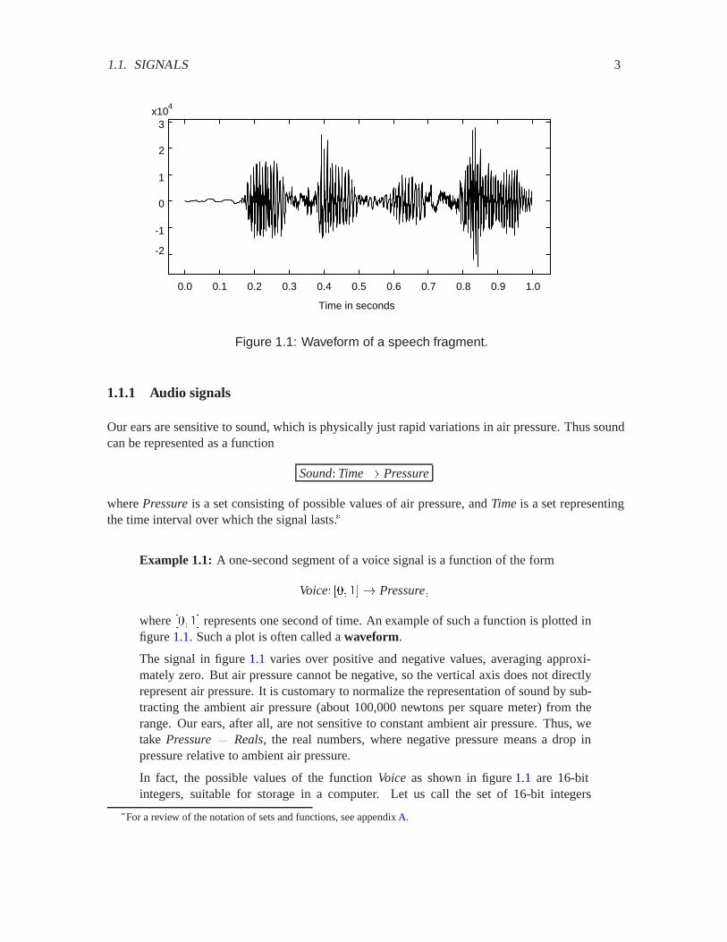
1.1. SIGNALS 3
-2
-1
0
1
2
3x10
4
0.0 0.1 0.2 0.3 0.4 0.5 0.6 0.7 0.8 0.9 1.0
Time in seconds
Figure 1.1: Waveform of a speech fragment.
1.1.1 Audio signals
Our ears are sensitive to sound, which is physically just rapid variations in air pressure. Thus soundcan be represented as a function
Sound�Time� Pressure
where Pressureis a set consisting of possible values of air pressure, and Timeis a set representingthe time interval over which the signal lasts.�
Example 1.1: A one-second segment of a voice signal is a function of the form
Voice� �� �� Pressure�
where �� � represents one second of time. An example of such a function is plotted infigure 1.1. Such a plot is often called a waveform.
The signal in figure 1.1 varies over positive and negative values, averaging approxi-mately zero. But air pressure cannot be negative, so the vertical axis does not directlyrepresent air pressure. It is customary to normalize the representation of sound by sub-tracting the ambient air pressure (about 100,000 newtons per square meter) from therange. Our ears, after all, are not sensitive to constant ambient air pressure. Thus, wetake Pressure� Reals, the real numbers, where negative pressure means a drop inpressure relative to ambient air pressure.
In fact, the possible values of the function Voice as shown in figure 1.1 are 16-bitintegers, suitable for storage in a computer. Let us call the set of 16-bit integers
�For a review of the notation of sets and functions, see appendix A.
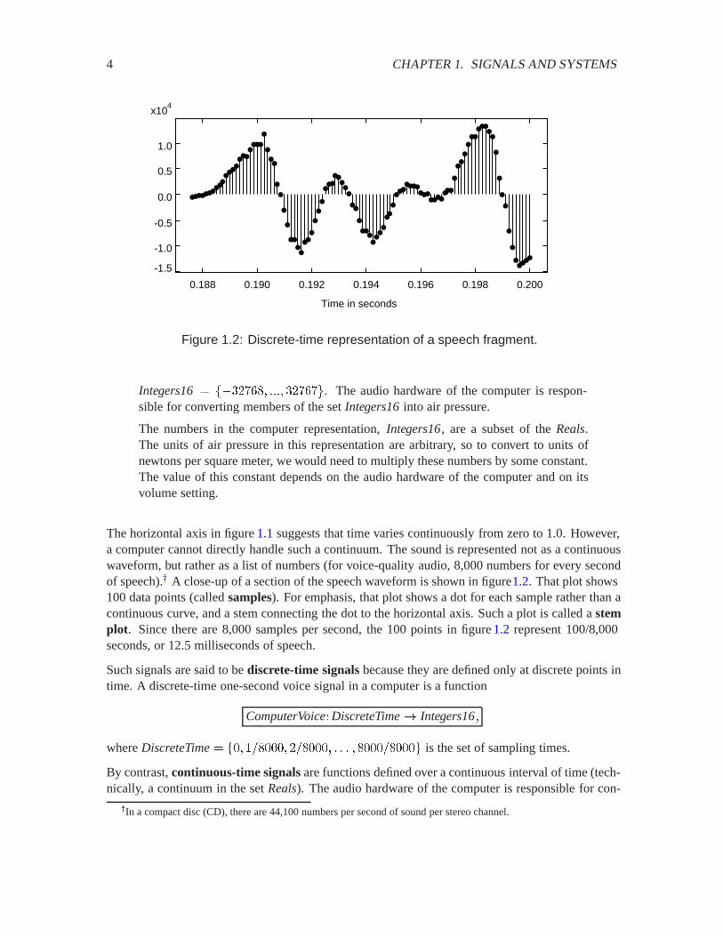
4 CHAPTER 1. SIGNALS AND SYSTEMS
-1.5
-1.0
-0.5
0.0
0.5
1.0
x104
0.188 0.190 0.192 0.194 0.196 0.198 0.200
Time in seconds
Figure 1.2: Discrete-time representation of a speech fragment.
Integers16� ����� �� ���� ��� �. The audio hardware of the computer is respon-sible for converting members of the set Integers16into air pressure.
The numbers in the computer representation, Integers16, are a subset of the Reals.The units of air pressure in this representation are arbitrary, so to convert to units ofnewtons per square meter, we would need to multiply these numbers by some constant.The value of this constant depends on the audio hardware of the computer and on itsvolume setting.
The horizontal axis in figure 1.1 suggests that time varies continuously from zero to 1.0. However,a computer cannot directly handle such a continuum. The sound is represented not as a continuouswaveform, but rather as a list of numbers (for voice-quality audio, 8,000 numbers for every secondof speech).� A close-up of a section of the speech waveform is shown in figure1.2. That plot shows100 data points (called samples). For emphasis, that plot shows a dot for each sample rather than acontinuous curve, and a stem connecting the dot to the horizontal axis. Such a plot is called a stemplot. Since there are 8,000 samples per second, the 100 points in figure 1.2 represent 100/8,000seconds, or 12.5 milliseconds of speech.
Such signals are said to be discrete-time signals because they are defined only at discrete points intime. A discrete-time one-second voice signal in a computer is a function
ComputerVoice�DiscreteTime� Integers16�
where DiscreteTime� �� ��� ���� � � � � ��� is the set of sampling times.
By contrast, continuous-time signals are functions defined over a continuous interval of time (tech-nically, a continuum in the set Reals). The audio hardware of the computer is responsible for con-
�In a compact disc (CD), there are 44,100 numbers per second of sound per stereo channel.
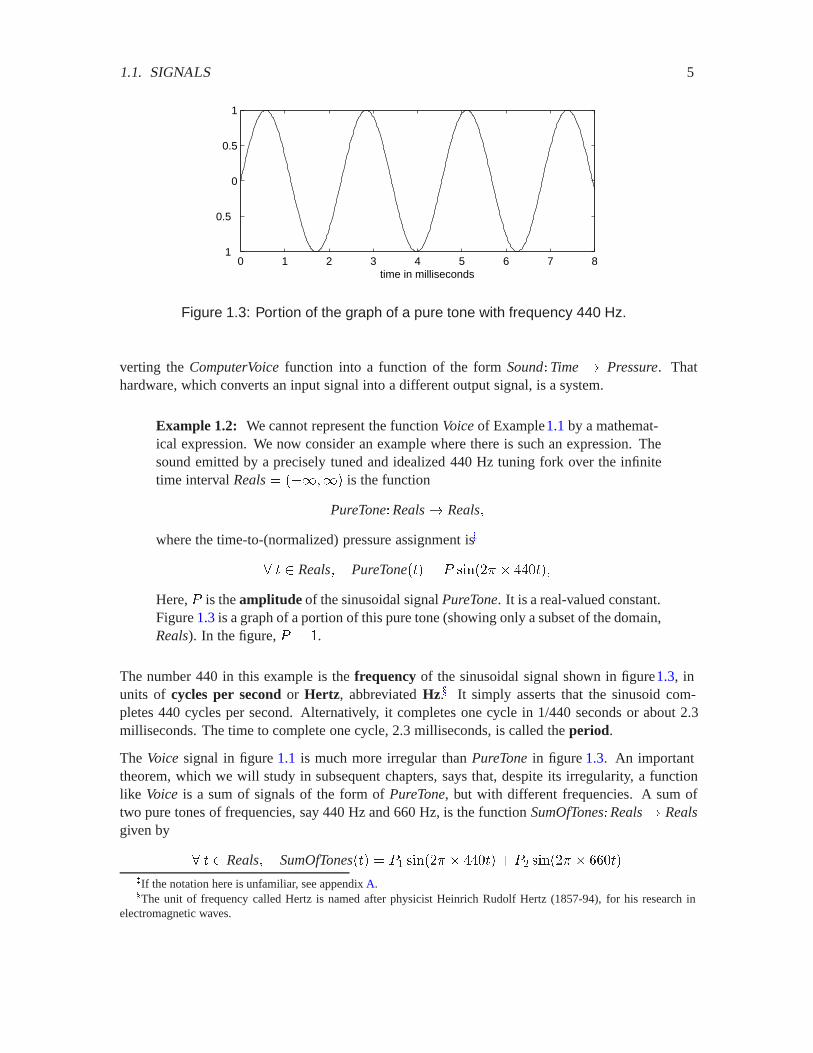
1.1. SIGNALS 5
0 1 2 3 4 5 6 7 81
0.5
0
0.5
1
time in milliseconds
Figure 1.3: Portion of the graph of a pure tone with frequency 440 Hz.
verting the ComputerVoicefunction into a function of the form Sound�Time� Pressure. Thathardware, which converts an input signal into a different output signal, is a system.
Example 1.2: We cannot represent the function Voiceof Example1.1 by a mathemat-ical expression. We now consider an example where there is such an expression. Thesound emitted by a precisely tuned and idealized 440 Hz tuning fork over the infinitetime interval Reals� ������ is the function
PureTone�Reals� Reals�
where the time-to-(normalized) pressure assignment is�
� Reals� PureTone�� � � ������ � ����
Here, � is the amplitude of the sinusoidal signal PureTone. It is a real-valued constant.Figure 1.3 is a graph of a portion of this pure tone (showing only a subset of the domain,Reals). In the figure, � � .
The number 440 in this example is the frequency of the sinusoidal signal shown in figure1.3, inunits of cycles per second or Hertz, abbreviated Hz.� It simply asserts that the sinusoid com-pletes 440 cycles per second. Alternatively, it completes one cycle in 1/440 seconds or about 2.3milliseconds. The time to complete one cycle, 2.3 milliseconds, is called the period.
The Voicesignal in figure 1.1 is much more irregular than PureTonein figure 1.3. An importanttheorem, which we will study in subsequent chapters, says that, despite its irregularity, a functionlike Voice is a sum of signals of the form of PureTone, but with different frequencies. A sum oftwo pure tones of frequencies, say 440 Hz and 660 Hz, is the function SumOfTones�Reals� Realsgiven by
� Reals� SumOfTones�� � �� ������ � ��� � �� ������ � ��If the notation here is unfamiliar, see appendix A.�The unit of frequency called Hertz is named after physicist Heinrich Rudolf Hertz (1857-94), for his research in
electromagnetic waves.
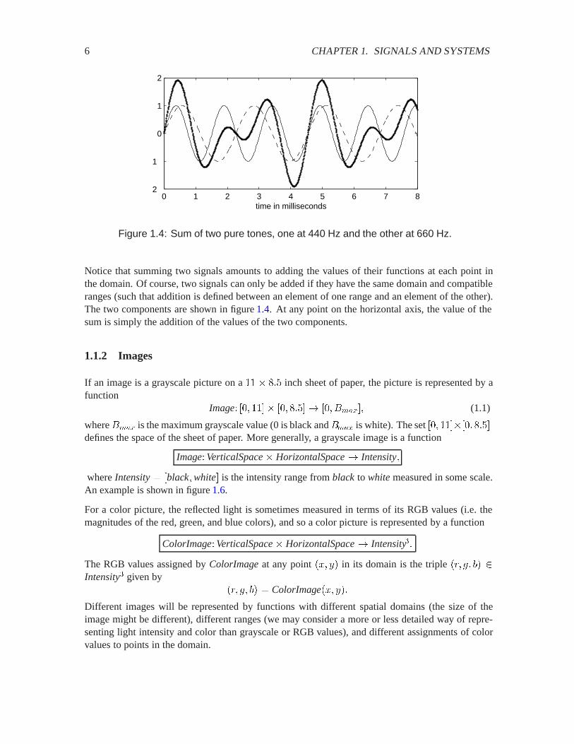
6 CHAPTER 1. SIGNALS AND SYSTEMS
0 1 2 3 4 5 6 7 82
1
0
1
2
time in milliseconds
Figure 1.4: Sum of two pure tones, one at 440 Hz and the other at 660 Hz.
Notice that summing two signals amounts to adding the values of their functions at each point inthe domain. Of course, two signals can only be added if they have the same domain and compatibleranges (such that addition is defined between an element of one range and an element of the other).The two components are shown in figure 1.4. At any point on the horizontal axis, the value of thesum is simply the addition of the values of the two components.
1.1.2 Images
If an image is a grayscale picture on a � ��� inch sheet of paper, the picture is represented by afunction
Image� �� � � �� ���� � �� ������ (1.1)
where ���� is the maximum grayscale value (0 is black and ���� is white). The set �� ���� ����defines the space of the sheet of paper. More generally, a grayscale image is a function
Image�VerticalSpace� HorizontalSpace� Intensity�
where Intensity� �black�white� is the intensity range from black to whitemeasured in some scale.An example is shown in figure 1.6.
For a color picture, the reflected light is sometimes measured in terms of its RGB values (i.e. themagnitudes of the red, green, and blue colors), and so a color picture is represented by a function
ColorImage�VerticalSpace� HorizontalSpace� Intensity��
The RGB values assigned by ColorImageat any point ��� �� in its domain is the triple ��� �� �� Intensity� given by
��� �� �� � ColorImage��� ���
Different images will be represented by functions with different spatial domains (the size of theimage might be different), different ranges (we may consider a more or less detailed way of repre-senting light intensity and color than grayscale or RGB values), and different assignments of colorvalues to points in the domain.

1.1. SIGNALS 7
Probing further: Household electrical power
In the U.S., household current is delivered on three wires, a neutral wire and twohot wires. The voltage between either hot wire and the neutral wire is around110 to 120 volts, RMS (root mean square, the square root of the average of thevoltage squared). The voltage between the two hot wires is around 220 to 240volts, RMS. The higher voltage is used for appliances that need more power, suchas air conditioners. Here, we examine exactly how this works.
The voltage between the hot wires and the neutral wire is sinusoidal with a fre-quency of 60 Hz. Thus, for one of the hot wires, it is a function ��Reals� Realswhere the domain represents time and the range represents voltage, and
� Reals� ��� � � ���� � ����
This 60 Hertz sinusoidal waveform completes one cycle in a period of � � seconds. Why is the amplitude 170 volts, rather than 120? Because the 120 voltageis RMS (root mean square). That is,
voltage�� �
�
� �
������ volts�
the square root of the average of the square of the voltage. This evaluates to 120.
The voltage between the second hot wire and the neutral wire is a function��Reals� Realswhere
� Reals� ��� � �� ���� � ��� � �����
It is the negative of the other voltage at any time . This sinusoidal signal is saidto have a phase shift of 180 degrees, or � radians, compared to the first sinusoid.Equivalently, it is said to be 180 degrees out of phase.
We can now see how to get the higher voltage for power-hungry appliances. Wesimply use the two hot wires rather than one hot wire and the neutral wire. Thevoltage between the two hot wires is the difference, a function ��Reals� Realswhere
� Reals� ��� � ���� ��� � �� ���� � ����
This corresponds to 240 volts RMS. A plot is shown in figure 1.5.
The neutral wire should not be confused with the ground wire in a three-prongplug. The ground wire is not connected to electrical company facilities. The neutralwire is. The ground wire is typically connected to the plumbing or some metallicconductor that goes underground. It is a safety feature to allow current to flow intothe earth rather than, say, through a person.
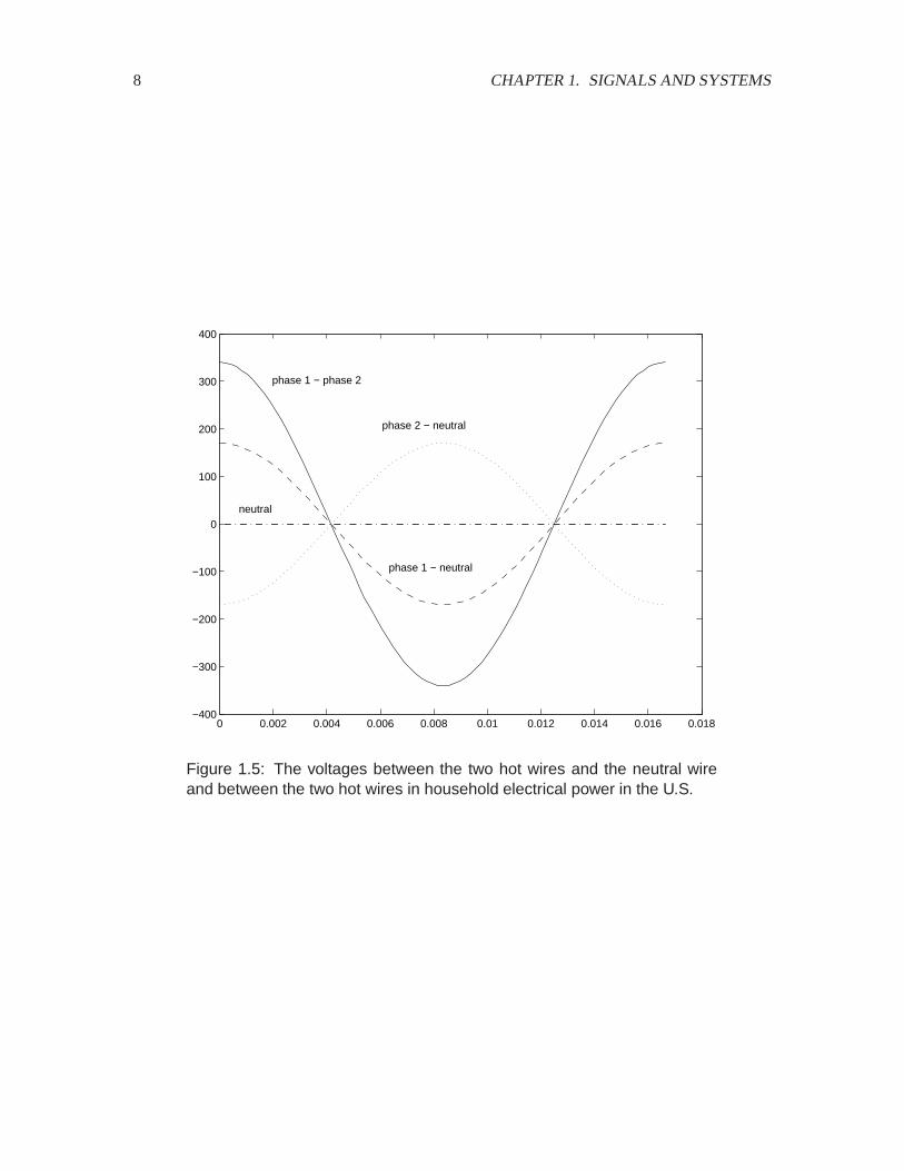
8 CHAPTER 1. SIGNALS AND SYSTEMS
0 0.002 0.004 0.006 0.008 0.01 0.012 0.014 0.016 0.018−400
−300
−200
−100
0
100
200
300
400
phase 1 − neutral
phase 2 − neutral
phase 1 − phase 2
neutral
Figure 1.5: The voltages between the two hot wires and the neutral wireand between the two hot wires in household electrical power in the U.S.

1.1. SIGNALS 9
Figure 1.6: Grayscale image on the left, and its enlarged pixels on the right.
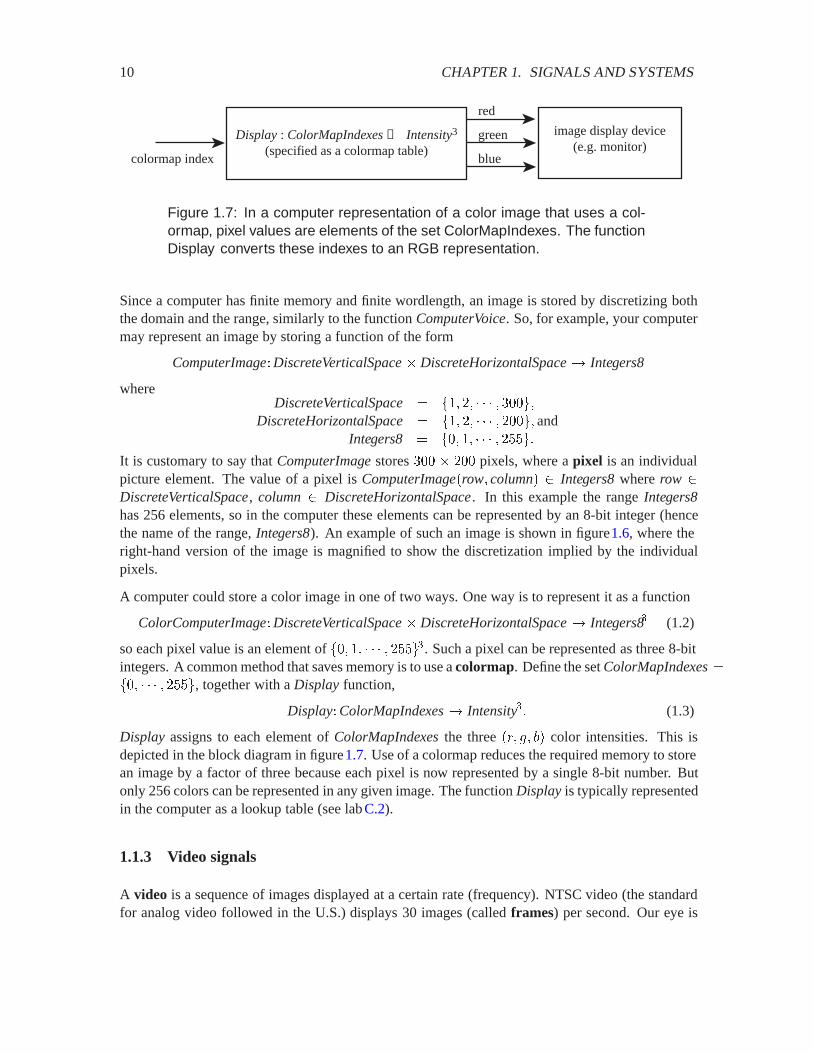
10 CHAPTER 1. SIGNALS AND SYSTEMS
Display : ColorMapIndexes → Intensity3
(specified as a colormap table)
image display device(e.g. monitor)
red
green
bluecolormap index
Figure 1.7: In a computer representation of a color image that uses a col-ormap, pixel values are elements of the set ColorMapIndexes. The functionDisplay converts these indexes to an RGB representation.
Since a computer has finite memory and finite wordlength, an image is stored by discretizing boththe domain and the range, similarly to the function ComputerVoice. So, for example, your computermay represent an image by storing a function of the form
ComputerImage�DiscreteVerticalSpace� DiscreteHorizontalSpace� Integers8
whereDiscreteVerticalSpace� �� �� � ��
DiscreteHorizontalSpace� �� �� � �� andIntegers8 � �� � � ����
It is customary to say that ComputerImagestores � � � pixels, where a pixel is an individualpicture element. The value of a pixel is ComputerImage�row� column� Integers8where row DiscreteVerticalSpace, column DiscreteHorizontalSpace. In this example the range Integers8has 256 elements, so in the computer these elements can be represented by an 8-bit integer (hencethe name of the range, Integers8). An example of such an image is shown in figure1.6, where theright-hand version of the image is magnified to show the discretization implied by the individualpixels.
A computer could store a color image in one of two ways. One way is to represent it as a function
ColorComputerImage�DiscreteVerticalSpace� DiscreteHorizontalSpace� Integers8� (1.2)
so each pixel value is an element of �� � � ����. Such a pixel can be represented as three 8-bitintegers. A common method that saves memory is to use a colormap. Define the set ColorMapIndexes��� � ���, together with a Display function,
Display�ColorMapIndexes� Intensity�� (1.3)
Display assigns to each element of ColorMapIndexesthe three ��� �� �� color intensities. This isdepicted in the block diagram in figure1.7. Use of a colormap reduces the required memory to storean image by a factor of three because each pixel is now represented by a single 8-bit number. Butonly 256 colors can be represented in any given image. The function Displayis typically representedin the computer as a lookup table (see lab C.2).
1.1.3 Video signals
A video is a sequence of images displayed at a certain rate (frequency). NTSC video (the standardfor analog video followed in the U.S.) displays 30 images (called frames) per second. Our eye is
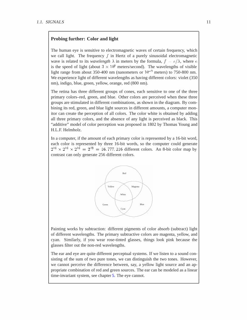
1.1. SIGNALS 11
Probing further: Color and light
The human eye is sensitive to electromagnetic waves of certain frequency, whichwe call light. The frequency � in Hertz of a purely sinusoidal electromagneticwave is related to its wavelength in meters by the formula, � � !� , where !is the speed of light (about � � � meters/second). The wavelengths of visiblelight range from about 350-400 nm (nanometers or �� meters) to 750-800 nm.We experience light of different wavelengths as having different colors: violet (350nm), indigo, blue, green, yellow, orange, red (800 nm).
The retina has three different groups of cones, each sensitive to one of the threeprimary colors–red, green, and blue. Other colors are perceived when these threegroups are stimulated in different combinations, as shown in the diagram. By com-bining its red, green, and blue light sources in different amounts, a computer mon-itor can create the perception of all colors. The color white is obtained by addingall three primary colors, and the absence of any light is perceived as black. This“additive” model of color perception was proposed in 1802 by Thomas Young andH.L.F. Helmholz.
In a computer, if the amount of each primary color is represented by a 16-bit word,each color is represented by three 16-bit words, so the computer could generate��� � ��� � ��� � �� � � ���� � different colors. An 8-bit color map bycontrast can only generate 256 different colors.
Red
Green Blue
Yellow Magenta
Cyan
White
Painting works by subtraction: different pigments of color absorb (subtract) lightof different wavelengths. The primary subtractive colors are magenta, yellow, andcyan. Similarly, if you wear rose-tinted glasses, things look pink because theglasses filter out the non-red wavelengths.
The ear and eye are quite different perceptual systems. If we listen to a sound con-sisting of the sum of two pure tones, we can distinguish the two tones. However,we cannot perceive the difference between, say, a yellow light source and an ap-propriate combination of red and green sources. The ear can be modeled as a lineartime-invariant system, see chapter 5. The eye cannot.

12 CHAPTER 1. SIGNALS AND SYSTEMS
0 1/30 2/30 3/30 n/30... ...
ImageSet
FrameTimes
Figure 1.8: Illustration of the function Video.
unable to distinguish between successive images displayed at this frequency, and so a TV broadcastappears to be continuously varying in time.
Thus the domain of a video signal is discrete time, FrameTimes� �� ��� ���� , and itsrange is a set of images, ImageSet. For analog video, each image in ImageSetis a function of theform
VideoFrame�DiscreteVerticalSpace� HorizontalSpace� Intensity��
An analog video signal is discretized in the vertical direction, but not in the horizontal direction.�
The image is composed of a set of horizontal lines called scan lines, where the intensity varies alongthe line. The horizontal lines are stacked vertically to form an image.
A video signal, therefore, is a function
Video�FrameTimes� ImageSet� (1.4)
For any time FrameTimes, the image Video�� ImageSetis displayed. The signal Video isillustrated in figure 1.8.
An alternative way of specifying a video signal is by the function Video� whose domain is a productset as follows:
Video��FrameTimes� DiscreteVerticalSpace� HorizontalSpace� Intensity��
Similarly to figure 1.8, we can depict Video� as in figure 1.9. The RGB value assigned to a point��� �� at time is
��� �� �� � Video��� �� ��� (1.5)
�This is a simplification. Most analog video images are interlaced, meaning that successive frames use different setsfor DiscreteVerticalSpaceso that scan lines in one frame lie in between the scan lines of the previous frame. Also, therange Intensity� has a curious structure that ensures compatibility between black-and-white and color television sets.
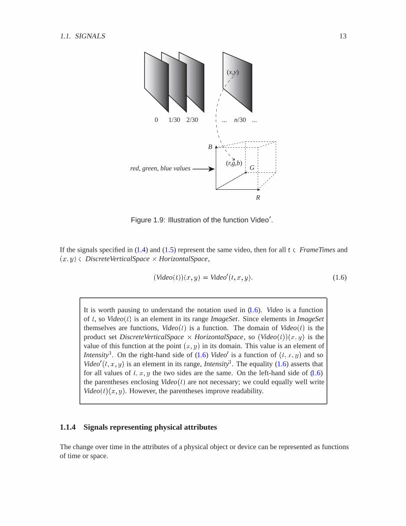
1.1. SIGNALS 13
0 1/30 2/30 n/30... ...
R
B
G(r,g,b)
(x,y)
red, green, blue values
Figure 1.9: Illustration of the function Video�.
If the signals specified in (1.4) and (1.5) represent the same video, then for all FrameTimesand��� �� DiscreteVerticalSpace� HorizontalSpace,
�Video������ �� � Video��� �� ��� (1.6)
It is worth pausing to understand the notation used in (1.6). Video is a functionof , so Video�� is an element in its range ImageSet. Since elements in ImageSetthemselves are functions, Video�� is a function. The domain of Video�� is theproduct set DiscreteVerticalSpace� HorizontalSpace, so �Video������ �� is thevalue of this function at the point ��� �� in its domain. This value is an element ofIntensity�. On the right-hand side of (1.6) Video� is a function of �� �� �� and soVideo��� �� �� is an element in its range, Intensity�. The equality (1.6) asserts thatfor all values of � �� � the two sides are the same. On the left-hand side of (1.6)the parentheses enclosing Video�� are not necessary; we could equally well writeVideo����� ��. However, the parentheses improve readability.
1.1.4 Signals representing physical attributes
The change over time in the attributes of a physical object or device can be represented as functionsof time or space.
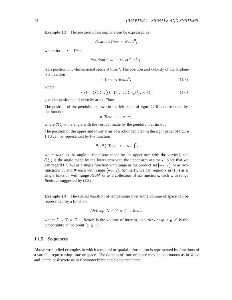
14 CHAPTER 1. SIGNALS AND SYSTEMS
Example 1.3: The position of an airplane can be expressed as
Position�Time� Reals��
where for all Time,
Position�� � ����� ���� ����
is its position in 3-dimensional space at time . The position and velocity of the airplaneis a function
��Time� Reals�� (1.7)
where��� � ����� ���� ���� "���� "��� "���� (1.8)
gives its position and velocity at Time.
The position of the pendulum shown in the left panel of figure 1.10 is represented bythe function
#�Time� ���� ���where #�� is the angle with the vertical made by the pendulum at time .
The position of the upper and lower arms of a robot depicted in the right panel of figure1.10 can be represented by the function
�#�� # ��Time� ���� ����
where #��� is the angle at the elbow made by the upper arm with the vertical, and# �� is the angle made by the lower arm with the upper arm at time . Note that wecan regard �#�� # � as a single function with range as the product set ���� ��� or as twofunctions #� and # each with range ���� ��. Similarly, we can regard � in (1.7) as asingle function with range Reals� or as a collection of six functions, each with rangeReals, as suggested by (1.8).
Example 1.4: The spatial variation of temperature over some volume of space can berepresented by a function
AirTemp�� � $ � % � Reals
where � � $ � % � Reals� is the volume of interest, and �&��'(��� �� �� is thetemperature at the point ��� �� ��.
1.1.5 Sequences
Above we studied examples in which temporal or spatial information is represented by functions ofa variable representing time or space. The domain of time or space may be continuous as in Voiceand Imageor discrete as in ComputerVoiceand ComputerImage.
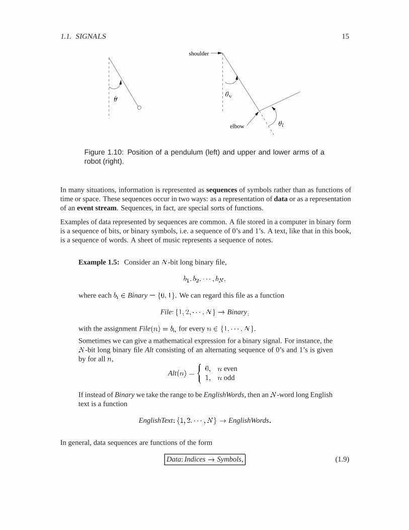
1.1. SIGNALS 15
elbow
shoulder
##�
#
Figure 1.10: Position of a pendulum (left) and upper and lower arms of arobot (right).
In many situations, information is represented as sequences of symbols rather than as functions oftime or space. These sequences occur in two ways: as a representation of data or as a representationof an event stream. Sequences, in fact, are special sorts of functions.
Examples of data represented by sequences are common. A file stored in a computer in binary formis a sequence of bits, or binary symbols, i.e. a sequence of 0’s and 1’s. A text, like that in this book,is a sequence of words. A sheet of music represents a sequence of notes.
Example 1.5: Consider an � -bit long binary file,
��� ��� � �� �
where each �� Binary� �� . We can regard this file as a function
File� �� �� � � � Binary�
with the assignment File��� � �� for every � �� � �.Sometimes we can give a mathematical expression for a binary signal. For instance, the� -bit long binary file Alt consisting of an alternating sequence of 0’s and 1’s is givenby for all �,
Alt��� �
�� � even� � odd
If instead of Binarywe take the range to be EnglishWords, then an � -word long Englishtext is a function
EnglishText� �� �� � � � EnglishWords�
In general, data sequences are functions of the form
Data� Indices� Symbols, (1.9)
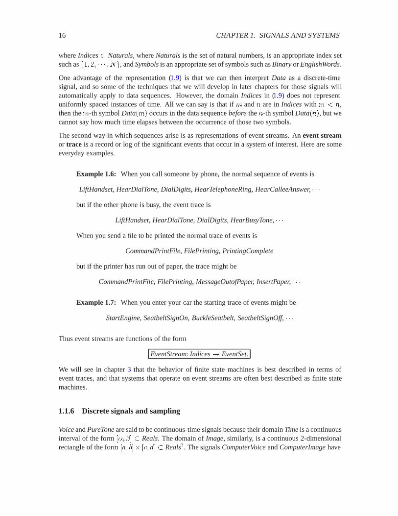
16 CHAPTER 1. SIGNALS AND SYSTEMS
where Indices� Naturals, where Naturalsis the set of natural numbers, is an appropriate index setsuch as �� �� � �, and Symbolsis an appropriate set of symbols such as Binaryor EnglishWords.
One advantage of the representation (1.9) is that we can then interpret Data as a discrete-timesignal, and so some of the techniques that we will develop in later chapters for those signals willautomatically apply to data sequences. However, the domain Indices in (1.9) does not representuniformly spaced instances of time. All we can say is that if ' and � are in Indiceswith ' ) �,then the '-th symbol Data�'� occurs in the data sequence beforethe �-th symbol Data���, but wecannot say how much time elapses between the occurrence of those two symbols.
The second way in which sequences arise is as representations of event streams. An event streamor trace is a record or log of the significant events that occur in a system of interest. Here are someeveryday examples.
Example 1.6: When you call someone by phone, the normal sequence of events is
LiftHandset, HearDialTone, DialDigits, HearTelephoneRing, HearCalleeAnswer,
but if the other phone is busy, the event trace is
LiftHandset, HearDialTone, DialDigits, HearBusyTone,
When you send a file to be printed the normal trace of events is
CommandPrintFile, FilePrinting, PrintingComplete
but if the printer has run out of paper, the trace might be
CommandPrintFile, FilePrinting, MessageOutofPaper, InsertPaper,
Example 1.7: When you enter your car the starting trace of events might be
StartEngine, SeatbeltSignOn, BuckleSeatbelt, SeatbeltSignOff,
Thus event streams are functions of the form
EventStream� Indices� EventSet.
We will see in chapter 3 that the behavior of finite state machines is best described in terms ofevent traces, and that systems that operate on event streams are often best described as finite statemachines.
1.1.6 Discrete signals and sampling
Voiceand PureToneare said to be continuous-time signals because their domain Timeis a continuousinterval of the form �*� +� � Reals. The domain of Image, similarly, is a continuous 2-dimensionalrectangle of the form ��� ��� �!� �� � Reals�. The signals ComputerVoiceand ComputerImagehave
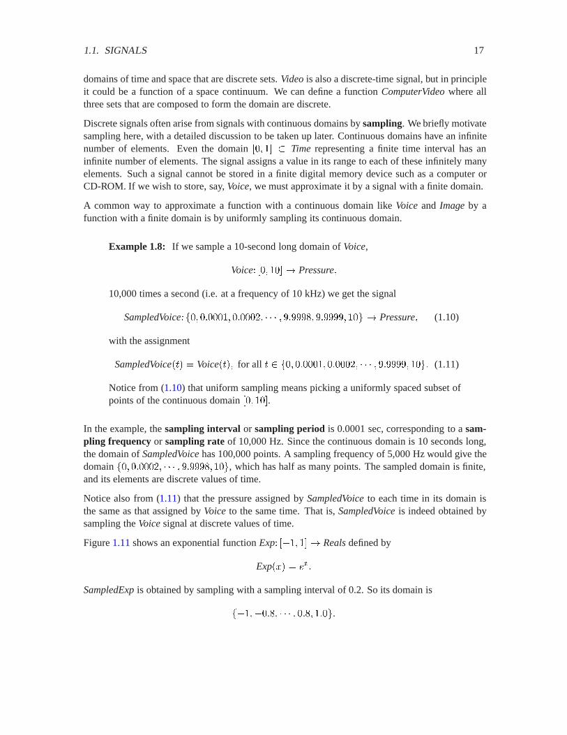
1.1. SIGNALS 17
domains of time and space that are discrete sets. Videois also a discrete-time signal, but in principleit could be a function of a space continuum. We can define a function ComputerVideowhere allthree sets that are composed to form the domain are discrete.
Discrete signals often arise from signals with continuous domains by sampling. We briefly motivatesampling here, with a detailed discussion to be taken up later. Continuous domains have an infinitenumber of elements. Even the domain �� � � Time representing a finite time interval has aninfinite number of elements. The signal assigns a value in its range to each of these infinitely manyelements. Such a signal cannot be stored in a finite digital memory device such as a computer orCD-ROM. If we wish to store, say, Voice, we must approximate it by a signal with a finite domain.
A common way to approximate a function with a continuous domain like Voice and Imageby afunction with a finite domain is by uniformly sampling its continuous domain.
Example 1.8: If we sample a 10-second long domain of Voice,
Voice� �� � � Pressure�
10,000 times a second (i.e. at a frequency of 10 kHz) we get the signal
SampledVoice� �� �� ��� � ������� ������� � Pressure� (1.10)
with the assignment
SampledVoice�� � Voice��� for all �� �� ��� � ������� � (1.11)
Notice from (1.10) that uniform sampling means picking a uniformly spaced subset ofpoints of the continuous domain �� �.
In the example, the sampling interval or sampling period is 0.0001 sec, corresponding to a sam-pling frequency or sampling rate of 10,000 Hz. Since the continuous domain is 10 seconds long,the domain of SampledVoicehas 100,000 points. A sampling frequency of 5,000 Hz would give thedomain �� ��� � ������� , which has half as many points. The sampled domain is finite,and its elements are discrete values of time.
Notice also from (1.11) that the pressure assigned by SampledVoiceto each time in its domain isthe same as that assigned by Voice to the same time. That is, SampledVoiceis indeed obtained bysampling the Voicesignal at discrete values of time.
Figure 1.11 shows an exponential function Exp� ��� �� Realsdefined by
Exp��� � ���
SampledExpis obtained by sampling with a sampling interval of 0.2. So its domain is
������� � ��� ��
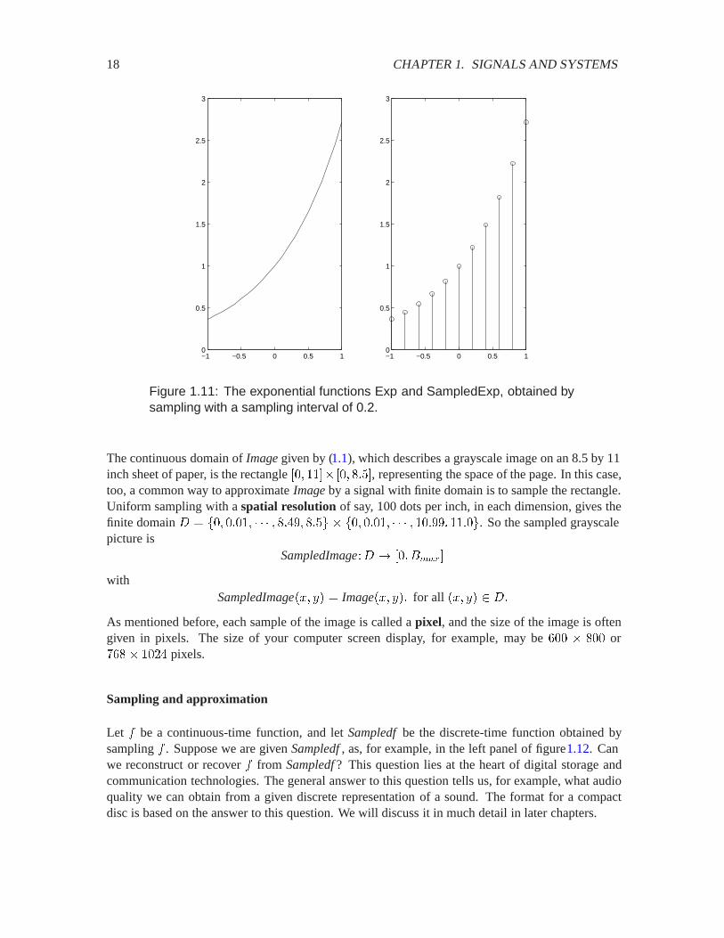
18 CHAPTER 1. SIGNALS AND SYSTEMS
−1 −0.5 0 0.5 10
0.5
1
1.5
2
2.5
3
−1 −0.5 0 0.5 10
0.5
1
1.5
2
2.5
3
Figure 1.11: The exponential functions Exp and SampledExp, obtained bysampling with a sampling interval of 0.2.
The continuous domain of Imagegiven by (1.1), which describes a grayscale image on an 8.5 by 11inch sheet of paper, is the rectangle �� �� �� ����, representing the space of the page. In this case,too, a common way to approximate Imageby a signal with finite domain is to sample the rectangle.Uniform sampling with a spatial resolution of say, 100 dots per inch, in each dimension, gives thefinite domain � � �� �� � ����� ��� � �� �� � ���� �. So the sampled grayscalepicture is
SampledImage�� � �� �����
withSampledImage��� �� � Image��� ��� for all ��� �� ��
As mentioned before, each sample of the image is called a pixel, and the size of the image is oftengiven in pixels. The size of your computer screen display, for example, may be � � or� � � �� pixels.
Sampling and approximation
Let � be a continuous-time function, and let Sampledfbe the discrete-time function obtained bysampling � . Suppose we are given Sampledf, as, for example, in the left panel of figure1.12. Canwe reconstruct or recover � from Sampledf? This question lies at the heart of digital storage andcommunication technologies. The general answer to this question tells us, for example, what audioquality we can obtain from a given discrete representation of a sound. The format for a compactdisc is based on the answer to this question. We will discuss it in much detail in later chapters.
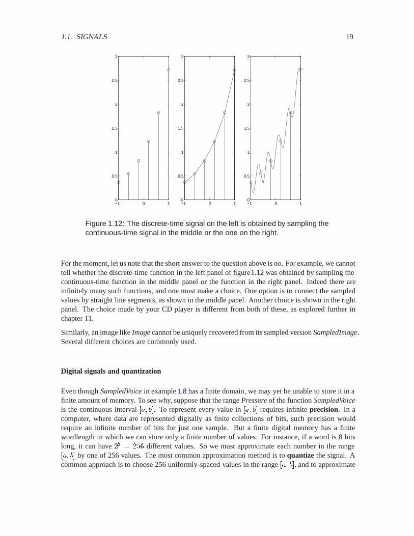
1.1. SIGNALS 19
−1 0 10
0.5
1
1.5
2
2.5
3
−1 0 10
0.5
1
1.5
2
2.5
3
−1 0 10
0.5
1
1.5
2
2.5
3
Figure 1.12: The discrete-time signal on the left is obtained by sampling thecontinuous-time signal in the middle or the one on the right.
For the moment, let us note that the short answer to the question above is no. For example, we cannottell whether the discrete-time function in the left panel of figure1.12 was obtained by sampling thecontinuous-time function in the middle panel or the function in the right panel. Indeed there areinfinitely many such functions, and one must make a choice. One option is to connect the sampledvalues by straight line segments, as shown in the middle panel. Another choice is shown in the rightpanel. The choice made by your CD player is different from both of these, as explored further inchapter 11.
Similarly, an image like Imagecannot be uniquely recovered from its sampled version SampledImage.Several different choices are commonly used.
Digital signals and quantization
Even though SampledVoicein example 1.8 has a finite domain, we may yet be unable to store it in afinite amount of memory. To see why, suppose that the range Pressureof the function SampledVoiceis the continuous interval ��� ��. To represent every value in ��� �� requires infinite precision. In acomputer, where data are represented digitally as finite collections of bits, such precision wouldrequire an infinite number of bits for just one sample. But a finite digital memory has a finitewordlength in which we can store only a finite number of values. For instance, if a word is 8 bitslong, it can have �� � �� different values. So we must approximate each number in the range��� �� by one of 256 values. The most common approximation method is to quantize the signal. Acommon approach is to choose 256 uniformly-spaced values in the range ��� ��, and to approximate

20 CHAPTER 1. SIGNALS AND SYSTEMS
−4 −3 −2 −1 0 1 2 3 4−1
−0.8
−0.6
−0.4
−0.2
0
0.2
0.4
0.6
0.8
1
Figure 1.13: PureTone (continuous curve), SampledPureTone (circles), andDigitalPureTone signals (x’s).
each value in ��� �� by the one of these 256 values that is closest. An alternative approximation,called truncation, is to choose the largest of the 256 values that is less than or equal to the desiredvalue.
Example 1.9: Figure 1.13 shows a PureTonesignal, SampledPureToneobtained aftersampling, and a quantized DigitalPureToneobtained using 4-bit or 16-level truncation.PureTonehas continuous domain and continuous range, while SampledPureTone(de-picted with circles) has discrete domain and continuous range, and DigitalPureTone(depicted with x’s) has discrete domain and discrete range. Only the last of these canbe precisely represented on a computer.
It is customary to call a signal with continuous domain and continuous range like PureToneananalog signal, and a signal with discrete domain and range, like �&�&�,PureTone, a digital signal.
Example 1.10: In digital telephones, voice is sampled every 125-sec, or at a samplingfrequency of 8,000 Hz. Each sample is quantized into an 8-bit word, or 256 levels. Thisgives an overall rate of �� � � � �� bits per second. The worldwide digitaltelephony network, therefore, is composed primarily of channels capable of carrying64,000 bits per second, or multiples of this (so that multiple telephone channels can becarried together). In cellular phones, voice samples are further compressed to bit ratesof 8,000 to 32,000 bits per second.

1.2. SYSTEMS 21
1.2 Systems
Systems are functions that transform signals. There are many reasons for transforming signals. Asignal carries information. A transformed signal may carry the same information in a different way.For example, in a live concert, music is represented as sound. A recording system may convertthat sound into a pattern of magnetic fields on a magnetic tape. The original signal, the sound, isdifficult to preserve for posterity. The magnetic tape has a more persistent representation of thesame information. Thus, storage is one of the tasks accomplished by systems.
A system may transform a signal into a form that is more convenient for transmission. Soundsignals cannot be carried by the Internet. There is simply no physical mechanism in the Internetfor transporting rapid variations in air pressure. The Internet provides instead a mechanism fortransporting sequences of bits. A system must convert a sound signal into a sequence of bits. Sucha system is called an encoder or coder. At the far end, of course, a decoder is needed to convertthe sequence back into sound. When a coder and a decoder are combined into the same physicaldevice, the device is often called a codec.
A system may transform a signal to hide its information so that snoops do not have access to it. Thisis called encryption. To be useful, we need matching decryption.
A system may enhance a signal by emphasizing some of the information it carries and deempha-sizing some other information. For example, an audio equalizer may compensate for poor roomacoustics by reducing the magnitude of certain low frequencies that happen to resonate in the room.In transmission, signals are often degraded by noise or distorted by physical effects in the transmis-sion medium. A system may attempt to reduce the noise or reverse the distortion. When the signalis carrying digital information over a physical channel, the extraction of the digital information fromthe degraded signal is called detection.
Systems are also designed to control physical processes such as the heating in a room, the ignition inan automobile engine, the flight of an aircraft. The state of the physical process (room temperature,cylinder pressure, aircraft speed) is sensed. The sensed signal is processed to generate signals thatdrive actuators, such as motors or switches. Engineers design a system called the controller which,on the basis of the processed sensor signal, determines the signals that control the physical process(turn the heater on or off, adjust the ignition timing, change the aircraft flaps) so that the process hasthe desired behavior (room temperature adjusts to the desired setting, engine delivers more torque,aircraft descends smoothly).
Systems are also designed for translation from one format to another. For example, a commandsequence from a musician may be transformed into musical sounds. Or the detection of risk ofcollision in an aircraft might be translated into control signals that perform evasive maneuvers.
1.2.1 Systems as functions
Consider a system . that transforms input signal � into output signal �. The system is a function,so � � .���. Suppose ��� � � is a signal with domain � and range �. For example, � might be
22 CHAPTER 1. SIGNALS AND SYSTEMS
a sound, ��Reals� Pressure. The domain of . is the set � of all such sounds, which we write
� � �� � �� � �� � ��� � � (1.12)
This notation reads “� , also written �� � ��, is the set of all � such that � is a function from �to �.” This set is called a signal space or function space. A signal or function space is a set of allfunctions with a given domain and range.
Example 1.11: The set of all sound segments with duration [0,1] and range Pressureis written
��� � � Pressure��
Notice that square brackets are used for both a subset of reals, as in �� �, and for afunction space, as in �� � ��, although obviously the meanings of these two notationsare very different.
The set ImageSetconsidered in section 1.1.3 is the function space
ImageSet� �DiscreteVerticalSpace� HorizontalSpace� Intensity���
Since this is a set, we can define functions that use it as a domain or range, as we havedone above with
Video�FrameTimes� ImageSet�
Similarly, the set of all binary files of length � is
BinaryFiles� �Indices� Binary��
where Indices� �� � �.
A system . is a function mapping a signal space into a signal space,
.� �� � ��� ��� � ����
Systems, therefore, are much like signals, except that their domain and range are both signal spaces.Thus, if � �� � �� and � � .���, then it must be that � ��� � ���. Furthermore, if � is anelement of ��, � ��, then
���� � .������ � �.������� ���
The parentheses around .��� in �.������� are not necessary, but may improve readability.
1.2.2 Telecommunications systems
We give some examples of systems that occur in or interact with the global telecommunications net-work. This network is unquestionably one of the most remarkable accomplishments of humankind.It is astonishingly complex, composed of hundreds of distinct corporations and linking billions ofpeople. We often think of it in terms of its basic service, POTS, or plain-old telephone service.
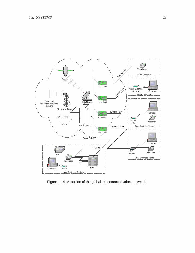
1.2. SYSTEMS 23
The globaltelecommunications
network
Cable
Optical Fiber
Home Customer
Small Business/Home
Small Business/Home
Large Business Customer
ISDNModem
Telephone
Computer
Modem
Fax
Telephone
Computer PBX
Satellite
Public Switch
T1 line
Line Card
Microwave Tower
DSL Card
ISDN card
Satellite dish
DSLModem
Telephone
Computer
Twisted
Pair
Twisted Pair
Twisted Pair
Coax Cable
Home Customer
Telephone
Line Card
Twisted
Pair
Voiceband DataModem Computer
Figure 1.14: A portion of the global telecommunications network.

24 CHAPTER 1. SIGNALS AND SYSTEMS
POTS
voice-like signal
TelephoneLine Card
voice-like signal
Network
Line CardTelephone
Figure 1.15: Abstraction of plain-old telephone service (POTS).
POTS is a voice service, but the telephone network is in fact a global, high-speed digital networkthat carries not just voice, but also video, images, and computer data, including much of the trafficin the Internet.
Figure 1.14 depicts a small portion of the global telecommunications network. POTS service isrepresented at the upper right, where a twisted pair of copper wires connects a central office toa home telephone. This twisted pair is called the local loop or subscriber line. At the centraloffice, the twisted pair is connected to a line card, which usually converts the signal from thetelephone immediately into digital form. The line card, in turn, is connected to a switch, whichroutes incoming and outgoing telephone connections. The Berkeley central office is located onBancroft, between Oxford and Shattuck.
The digital representation of a voice signal, a sequence of bits, is routed through the telephonenetwork. Usually it is combined with other bit sequences, which are other voices or computer data,and sent over high-speed links implemented with optical fiber, microwave radio, coaxial cable, orsatellites.
Of course, a telephone conversation usually involves two parties, so the network delivers to the sameline card a digital sequence representing the far-end speaker. That digital sequence is decoded anddelivered to the telephone via the twisted pair. The line card, therefore, includes a codec.
The telephone itself, of course, is a system. It transforms the electrical signal that propagates downthe twisted pair into a sound signal, and transforms a local sound signal into an electrical signal thatcan propagate down the twisted pair.
POTS can be abstracted as shown in figure 1.15. The entire network is reduced to a model thataccepts an electrical representation of a voice signal and transports it to a remote telephone. In thisabstraction, the digital nature of the telephone network is irrelevant. The system simply transports(and degrades somewhat) a voice signal.
DTMF
Even in POTS, not all of the information transported is voice. At a minimum, the telephone needsto be able to convey to the central office a telephone number in order to establish a connection. Atelephone number is not a voice signal. It is intrinsically discrete. Since the system is designed
1.2. SYSTEMS 25
Probing further: Wireless communication
Recently, the telephone network has been freeing itself of its dependence on wires.Cellular telephones, which came into widespread use in the 1990s, use radiowaves to connect a small, hand-held telephone to a nearby base station. The basestation connects directly to the telephone network.
There are three major challenges in the design of cellular networks. First, radiospectrum is scarce. Frequencies are allocated by regulatory bodies, often con-strained by international treaties. Finding frequencies for new technologies is dif-ficult. Thus, wireless communication devices have to be efficient in their use ofthe available frequencies. Second, the power available to drive a cellular phone islimited. Cellular phones must operate for reasonably long periods of time usingonly small batteries that fit easily within the handset. Although battery technologyhas been improving, the power that these batteries can deliver severely limits therange of a cellular phone (how far it can be from a base station) and the processingcomplexity (the microprocessors in a cellular phone consume considerable power).Third, networking is complicated. In order to be able to route telephone calls to acellular phone, the network needs to know where the phone is (or more specifically,which base station is closest). Moreover, the network needs to support phone callsin moving vehicles, which implies that a phone may move out of range of one basestation and into the range of another during the course of a telephone call. Thenetwork must hand off the call seamlessly.
Although “radio telephones” have existed for a long time, particularly for maritimeapplications where wireline telephony is impossible, it was the cellular conceptthat made it possible to offer radio telephony to large numbers of users. The con-cept is simple. Radio waves propagating along the surface of the earth lose powerapproximately proportionally to the inverse of the fourth power of distance. Thatis, if at distance � meters from a transmitter your receive / watts of radio power,then at distance �� you will receive approximately /�� � /� watts of radiopower. This fourth-power propagation loss was traditionally considered only to bea hindrance to wireless communication. It had to be overcome by greatly boostingthe transmitted power. The cellular concept turns this hindrance into an advantage.It observes that since the loss is so high, beyond a certain distance the same fre-quencies can be re-used without significant interference. Thus, the service area isdivided into cells. A second benefit of the cellular concept is that, at least in urbanareas, a cellular phone is never far from a base station. Thus, it does not need totransmit a high-power radio signal to reach a base station. This makes it possibleto operate on a small battery.
26 CHAPTER 1. SIGNALS AND SYSTEMS
Probing further: LEO telephony
Ideally, a cellular phone, with its one phone number, could be called anywhere inthe world, wherever it happens to be, without the caller needing to know whereit is. The technological and organizational infrastructure is evolving to make thispossible. When a phone “roams” out of its primary service area, it negotiates withthe local service provider in a new area for service. If that service provider hasa business agreement with the customer’s main service provider, then it providesservice. This requires complex networking so that telephone calls to the customerare routed to the correct locale.
However, digital cellular service, particularly in the US, remains spotty, with manyrural areas not served. Providing such service by installing base stations will be ex-pensive. Moreover, marine service away from coastlines is technically impossiblewith cellular technology.
One candidate technology for truly global telephony services is based on low-earth-orbit (LEO) satellites. One such project (now bankrupt) is the Iridium project,spearheaded by Motorola, and so named because in the initial conception, therewould be 77 satellites. The iridium atom has 77 electrons. The idea is that enoughsatellites are put into orbit that one is always near enough to communicate witha hand-held telephone. When the orbit is low enough that a hand-held telephonecan reach the satellite (a few hundred kilometers above the surface of the earth),the satellites move by fairly quickly. As a consequence, during the course of atelephone conversation, the connection may have to be handed off from one satelliteto another. In addition, in order to be able to serve enough users simultaneously,each satellite has to re-use frequencies according to the cellular concept. To do that,it focuses multiple beams on the surface of the earth using multi-element antennaarrays.
As of this writing, this approach has not yet proved economically viable. Theinvestment already has been huge, with at least one high-profile bankruptcy already,so the risks are high. Better networking of terrestrial cellular services may provideformidable competition, particularly as service improves to rural areas. The LEOapproach, however, has one advantage that terrestrial services cannot hope to matchanytime soon: truly worldwide service. The satellites provide service essentiallyeverywhere, even in remote wilderness areas and at sea.
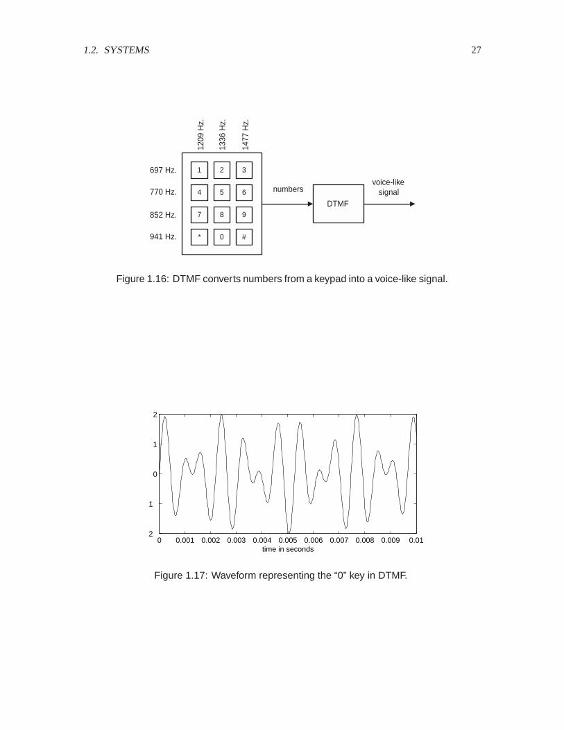
1.2. SYSTEMS 27
DTMF
numbersvoice-like
signal
1 2 3
4 5 6
7 8 9
* 0 #
697 Hz.
770 Hz.
852 Hz.
941 Hz.
1209
Hz.
1336
Hz.
1477
Hz.
Figure 1.16: DTMF converts numbers from a keypad into a voice-like signal.
0 0.001 0.002 0.003 0.004 0.005 0.006 0.007 0.008 0.009 0.012
1
0
1
2
time in seconds
Figure 1.17: Waveform representing the “0” key in DTMF.
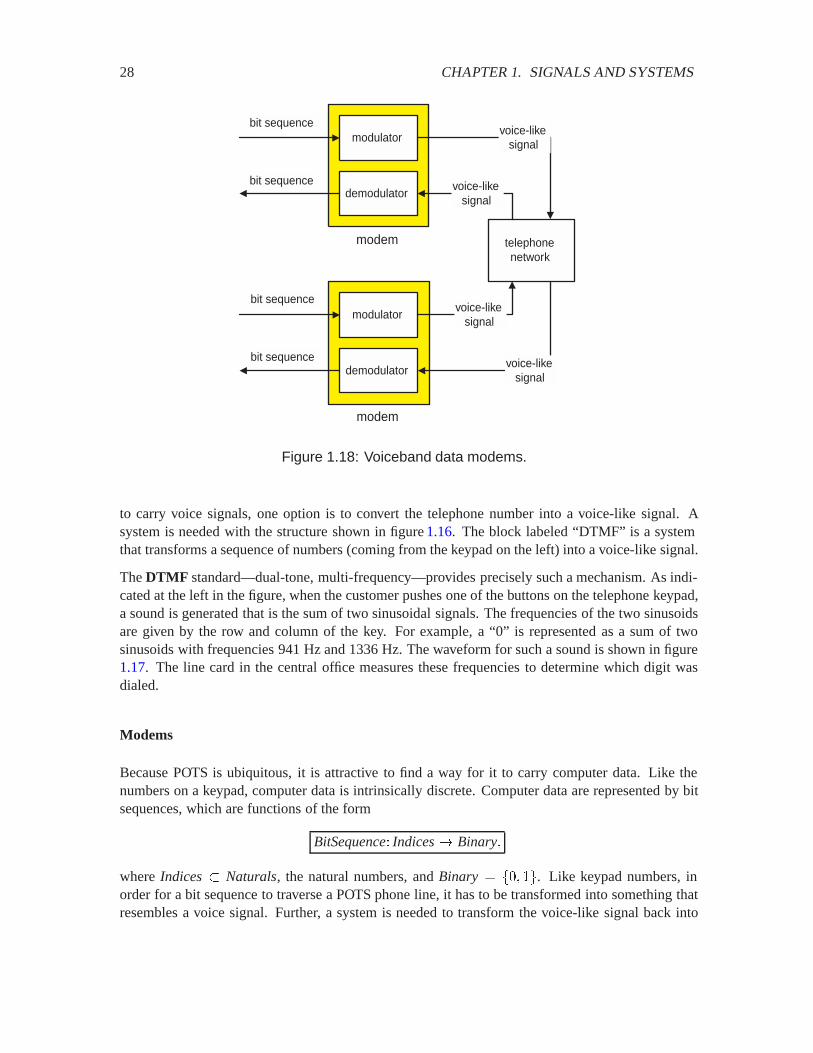
28 CHAPTER 1. SIGNALS AND SYSTEMS
modulatorbit sequence
telephonenetwork
demodulatorbit sequence
modem
voice-likesignal
voice-likesignal
modulatorbit sequence
demodulatorbit sequence
modem
voice-likesignal
voice-likesignal
Figure 1.18: Voiceband data modems.
to carry voice signals, one option is to convert the telephone number into a voice-like signal. Asystem is needed with the structure shown in figure 1.16. The block labeled “DTMF” is a systemthat transforms a sequence of numbers (coming from the keypad on the left) into a voice-like signal.
The DTMF standard—dual-tone, multi-frequency—provides precisely such a mechanism. As indi-cated at the left in the figure, when the customer pushes one of the buttons on the telephone keypad,a sound is generated that is the sum of two sinusoidal signals. The frequencies of the two sinusoidsare given by the row and column of the key. For example, a “0” is represented as a sum of twosinusoids with frequencies 941 Hz and 1336 Hz. The waveform for such a sound is shown in figure1.17. The line card in the central office measures these frequencies to determine which digit wasdialed.
Modems
Because POTS is ubiquitous, it is attractive to find a way for it to carry computer data. Like thenumbers on a keypad, computer data is intrinsically discrete. Computer data are represented by bitsequences, which are functions of the form
BitSequence� Indices� Binary�
where Indices� Naturals, the natural numbers, and Binary � �� . Like keypad numbers, inorder for a bit sequence to traverse a POTS phone line, it has to be transformed into something thatresembles a voice signal. Further, a system is needed to transform the voice-like signal back into
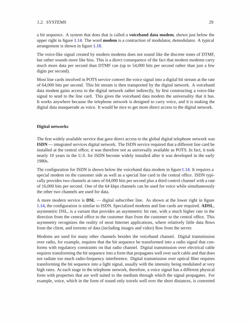
1.2. SYSTEMS 29
a bit sequence. A system that does that is called a voiceband data modem, shown just below theupper right in figure 1.14. The word modem is a contraction of modulator, demodulator. A typicalarrangement is shown in figure 1.18.
The voice-like signal created by modern modems does not sound like the discrete tones of DTMF,but rather sounds more like hiss. This is a direct consequence of the fact that modern modems carrymuch more data per second than DTMF can (up to 54,000 bits per second rather than just a fewdigits per second).
Most line cards involved in POTS service convert the voice signal into a digital bit stream at the rateof 64,000 bits per second. This bit stream is then transported by the digital network. A voicebanddata modem gains access to the digital network rather indirectly, by first constructing a voice-likesignal to send to the line card. This gives the voiceband data modem the universality that it has.It works anywhere because the telephone network is designed to carry voice, and it is making thedigital data masquerade as voice. It would be nice to get more direct access to the digital network.
Digital networks
The first widely available service that gave direct access to the global digital telephone network wasISDN — integrated services digital network. The ISDN service required that a different line card beinstalled at the central office; it was therefore not as universally available as POTS. In fact, it tooknearly 10 years in the U.S. for ISDN become widely installed after it was developed in the early1980s.
The configuration for ISDN is shown below the voiceband data modem in figure1.14. It requires aspecial modem on the customer side as well as a special line card in the central office. ISDN typi-cally provides two channels at rates of 64,000 bits per second plus a third control channel with a rateof 16,000 bits per second. One of the 64 kbps channels can be used for voice while simultaneouslythe other two channels are used for data.
A more modern service is DSL — digital subscriber line. As shown at the lower right in figure1.14, the configuration is similar to ISDN. Specialized modems and line cards are required. ADSL,asymmetric DSL, is a variant that provides an asymmetric bit rate, with a much higher rate in thedirection from the central office to the customer than from the customer to the central office. Thisasymmetry recognizes the reality of most Internet applications, where relatively little data flowsfrom the client, and torrents of data (including images and video) flow from the server.
Modems are used for many other channels besides the voiceband channel. Digital transmissionover radio, for example, requires that the bit sequence be transformed into a radio signal that con-forms with regulatory constraints on that radio channel. Digital transmission over electrical cablerequires transforming the bit sequence into a form that propagates well over such cable and that doesnot radiate too much radio-frequency interference. Digital transmission over optical fiber requirestransforming the bit sequence into a light signal, usually with the intensity being modulated at veryhigh rates. At each stage in the telephone network, therefore, a voice signal has a different physicalform with properties that are well suited to the medium through which the signal propagates. Forexample, voice, which in the form of sound only travels well over the short distances, is converted

30 CHAPTER 1. SIGNALS AND SYSTEMS
to an electrical signal that carries well over copper wires for the few kilometers. Copper wires, how-ever, are not as well matched for long distances as optical fiber. Most long distance communicationchannels today use optical fiber, although satellites still have certain advantages.
Signal degradation
A voice received via the telephone network is different from the original in several respects. Thesedifferences can be modeled by a system that degrades the voice signal.
First, there is a loss of information because of sampling and quantization in the encoder, as discussedin the section 1.1.6. Moreover, the media that carry the signal, such as the twisted pair, are notperfect. They distort the signal. One cause of distortion is addition of noise to the signal. Noise, bydefinition, is any undesired component in the signal. Noise in the telephone network is sometimesaudible as background hiss, or as crosstalk, i.e., leakage from other telephone channels into yourown. Another degradation is that the medium attenuates the signal, and this attenuation depends onthe signal frequency. The line card, in particular, usually contains a bandlimiting filter that discardsthe high frequency components of the signal. This is why telephone channels do not transport musicwell. Finally, the signal propagates over a physical medium at a finite speed, bounded by the speedof light, and so there is a delay between the time you say something and the time when the personat the other end hears what you say. Light travels through 1 km of optical fiber in approximately 5-s, so the 5,000 km between Berkeley and New York causes a delay of about 25 ms, which is noteasily perceptible.
Communications engineering is concerned with how to minimize the degradation for all kinds ofcommunication systems, including radio, TV, cellular phones, and computer networks (such as theInternet).
1.2.3 Audio storage and retrieval
We have seen how audio signals can be represented as sequences of numbers. Digital audio storageand retrieval is all about finding a physical and persistent representation for these numbers. Thesenumbers can be converted into a single sequence of bits (binary digits) and then “printed” ontosome physical medium from which they can later be read back. The transformation of sound intoits persistent representation can be modeled as a system, as can the reverse or playback process.
Example 1.12: In the case of compact discs (CDs), the physical medium is a layer ofaluminum on a platter into which tiny pits are etched. In the playback device, a laser
� A phone conversation relayed by satellite has a much larger delay. Most satellites traditionally used in the telecom-munications network are geosynchronous, meaning that they hover at the same point over the surface of the earth. To dothat, they have to orbit at a height of 22,300 miles or 35,900 kilometers. It takes a radio signal about 120 ms to traversethat distance; since a signal has to go up and back, there is an end-to-end delay of at least 240 ms (not counting delays inthe electronics). If you are using this channel for a telephone conversation, then the round-trip delay from when you saysomething to when you get a reaction is a minimum of 480 ms. This delay can be quite annoying, impeding your abilityto converse until you got used to it. If you use Internet telephony, the delays are even larger, and they can be irregulardepending upon how congested the Internet is when you call.

1.2. SYSTEMS 31
Probing further: Encrypted speech
Pairs of modems are used at opposite ends of a telephone connection, each with atransmitter and a receiver to achieve bidirectional (called full duplex) communica-tion. Once such modems are in place, and once they have been connected via thetelephone network, then they function as a bidirectional “bit pipe.” That bit pipe isthen usable by other systems, such as your computer.
One of the strangest uses is to transmit digitally represented and encrypted voicesignals. Here is a depiction of this relatively complicated arrangement:
modulatorbit sequence
telephonenetwork
demodulatorbit sequence
voice signalencoder
bit sequenceencryption
voice signaldecoder
bit sequencedecryption
modem
voice-likesignal
voice-likesignal
What is actually sent through the telephone network sounds like hiss, which byitself provides a modicum of privacy. Casual eavesdroppers will be unable to un-derstand the encoded speech. However, this configuration also provides protectionagainst sophisticated listeners. A listener that is able to extract the bit sequencefrom this sound will still not be able to reconstruct the voice signal because the bitsequence is encrypted.
Only one end is shown. The encoder and decoder, which convert voice signals toand from bit sequences, are fairly sophisticated systems, as are the encryption anddecryption systems. The fact that such an approach is cost effective has more to dowith economics and sociology than technology.
32 CHAPTER 1. SIGNALS AND SYSTEMS
aimed at the platter uses an interference pattern to determine whether or not a pit existsat a particular point in the platter. These pits, thus, naturally represent binary digits,since they can have two states (present or not present).
While a voiceband data modem converts bit sequences into voice-like signals, a musicalrecording studio does the reverse, creating a representation of the sound that is a bitsequence,
RecordingStudio�Sounds� BitStreams�
There is a great deal of engineering in the details, however. For instance, CDs arevulnerable to surface defects, which may arise in manufacturing or in the hands ofthe user. These defects may obscure some of the pits, or fool the reading laser intodetecting a pit where there is none. To guard against this, a very clever error-correctingcode called a Reed-Solomon code is used. The coding process can be viewed as afunction
Encoding�BitStreams� RedundantBitStreams�
where RedundantBitStreams� BitStreamsis the set of all possible encoded bit se-quences. These bit sequences are redundant, in that they contain more bits than arenecessary to represent the original bit sequence. The extra bits are used to detect er-rors, and (sometimes) to correct them. Of course, if the surface of the CD is too badlydamaged, even this clever scheme fails, and the audio data will not be recoverable.
CDs also contain meta data, which is extra information about the audio signal. Thisinformation allows the CD player to identify the start of a musical number and itslength, and sometimes the title and the artist.
The CD format can also be used to contain purely digital data. Such a CD is called aCD ROM (read-only memory). It is called this because, like a computer memory, itcontains digital information. But unlike a computer memory, that information cannotbe modified.
DVD (digital video discs) take this concept much further, including much more metadata. They may eventually replace CDs. They are entirely compatible, in that they cancontain exactly the same audio data that a CD can. DVD players can play CDs, but notthe reverse, however. DVDs can also contain digital video information and, in fact, anyother digital data. DAT (digital audio tape) is also a competitor to CDs, but has failedto capture much of a market.
1.2.4 Modem negotiation
A very different kind of system is the one that manages the establishment of a connection betweentwo voiceband data modems. These two modems are at physically different locations, are proba-bly manufactured by different manufacturers, and possibly use different communication standards.Both modems convert bit streams to and from voice-like signals, but other than that, they do nothave much in common.
When a connection is established through the telephone network, the answering modem emits atone that announces “I am a modem.” The initiating modem listens for this tone, and if it fails to

1.2. SYSTEMS 33
detect it, assumes that no connection can be established and hangs up. If it does detect the tone, thenit answers with a voice-like signal that announces “I am a modem that can communicate accordingto ITU standard �,” where � is one of the many modem standard published by the InternationalTelecommunication Union, or ITU.
The answering modem may or may not recognize the signal from the initiating modem. The initi-ating modem, for example, may be a newer modem using a standard that was established after theanswering modem was manufactured. If the answering modem does recognize the signal, then it re-sponds with a signal that says “good, I too can communication using standard �, so let’s get started.”Otherwise, it remains silent. The initiating modem, if it fails to get a response, tries another signal,announcing “I am a modem that can communicate according to ITU standard �,” where � is typi-cally now an older (and slower) standard. This process continues until the two modems agree on astandard.
Once agreement is reached, the modems need to make measurements of the telephone channel tocompensate for its distortion. They do this by sending each other pre-agreed signals called trainingsignals, defined by the standard. The training signal is distorted by the channel, and, since thereceiving modem knows the signal, it can measure the distortion. It uses this measurement to set upa device called an adaptive equalizer. Once both modems have completed their setup, they beginto send data to one another.
As systems go, modem negotiation is fairly complex. It involves both event sequences and voice-like signals. The voice like signals need to be analyzed in fairly sophisticated ways, sometimesproducing events in the event sequences. It will take this entire book to analyze all parts of thissystem. The handling of the event sequences will be treated using finite state machines, and thehandling of the voice-like signals will be treated using frequency-domain concepts and filtering.
1.2.5 Feedback control systems
Feedback control systems are composite systems where a plant embodies a physical process whosebehavior is guided by a control signal. A plant may be a mechanical device, such as the power trainof a car, or a chemical process, or an aircraft with certain inertial and aerodynamic properties, forexample. Sensors attached to the plant produce signals that are fed to the controller, which then gen-erates the control signal. This arrangement, where the plant feeds the controller and the controllerfeeds the plant, is a complicated sort of composite system called a feedback control system. It hasextremely interesting properties which we will explore in much more depth in subsequent chapters.
In this section, we construct a model of a feedback control system using the syntax of block dia-grams. The model consists of several interconnected components. We will identify the input andoutput signals of each component and how the components are interconnected, and we will argueon the basis of a common-sense physics how the overall system will behave.
Example 1.13: Consider a forced air heating system, which heats a room in a home oroffice to a desired temperature. Our first task is to identify the individual componentsof the heating system. These are
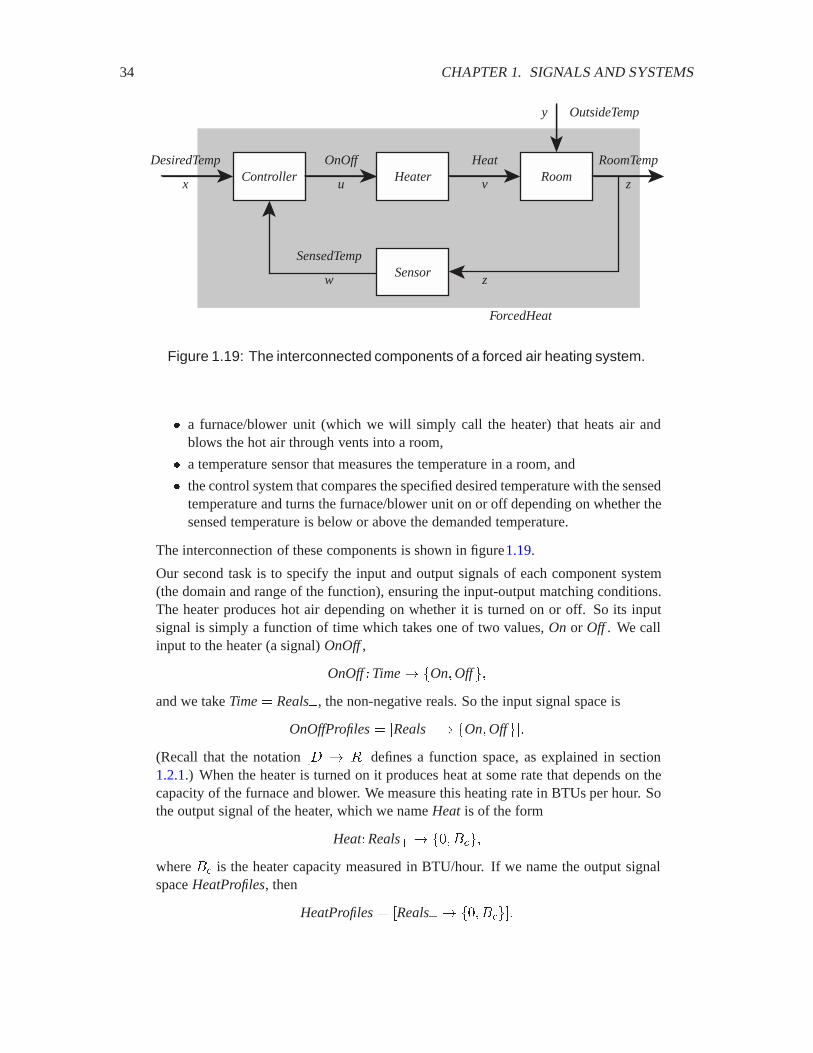
34 CHAPTER 1. SIGNALS AND SYSTEMS
Controller HeaterDesiredTemp
x
OnOff
u
Heat
vRoom
RoomTemp
z
SensorSensedTemp
w
OutsideTempy
z
ForcedHeat
Figure 1.19: The interconnected components of a forced air heating system.
� a furnace/blower unit (which we will simply call the heater) that heats air andblows the hot air through vents into a room,
� a temperature sensor that measures the temperature in a room, and
� the control system that compares the specified desired temperature with the sensedtemperature and turns the furnace/blower unit on or off depending on whether thesensed temperature is below or above the demanded temperature.
The interconnection of these components is shown in figure1.19.
Our second task is to specify the input and output signals of each component system(the domain and range of the function), ensuring the input-output matching conditions.The heater produces hot air depending on whether it is turned on or off. So its inputsignal is simply a function of time which takes one of two values, On or Off . We callinput to the heater (a signal) OnOff,
OnOff�Time� �On�Off�and we take Time� Reals�, the non-negative reals. So the input signal space is
OnOffProfiles� �Reals� � �On�Off��(Recall that the notation �� � �� defines a function space, as explained in section1.2.1.) When the heater is turned on it produces heat at some rate that depends on thecapacity of the furnace and blower. We measure this heating rate in BTUs per hour. Sothe output signal of the heater, which we name Heat is of the form
Heat�Reals� � �� ���where �� is the heater capacity measured in BTU/hour. If we name the output signalspace HeatProfiles, then
HeatProfiles� �Reals� � �� ����

1.2. SYSTEMS 35
Thus the Heatersystem is described by a function
Heater�OnOffProfiles� HeatProfiles� (1.13)
Common-sense physics tells us that when the heater is turned on the room will begin towarm up and when the heater is turned off the room temperature will fall until it reachesthe outside temperature. So the room temperature depends on both the heat deliveredby the heater and the outside temperature. Thus the input signal to the room is the pair�Heat�OutsideTemp�. We can take OutsideTempto be of the form
OutsideTemp�Reals� � �min�max��
where �min�max� is the range of possible outside temperatures, measured in degreesCelsius, say. The output signal of the room is of course the room temperature,
RoomTemp�Reals� � �min�max��
If we denoteOutsideTempProfiles� �Reals� � �min�max���
andRoomTempProfiles� �Reals� � �min�max���
then the behavior of the Roomsystem is described by a function
Room�HeatProfiles�OutsideTempProfiles� RoomTempProfiles (1.14)
In a similar manner, the Sensorsystem is described by a function
Sensor�RoomTempProfiles� SensedTempProfiles (1.15)
with input signal space RoomTempProfilesand output signal space
SensedTempProfiles� �Reals� � �min�max���
The Controller is described by the function
Controller�DesiredTempProfile� SensedTempProfile� OnOffProfile� (1.16)
whereDesiredTempProfiles� �Reals� � �min�max���
We have constructed a model where the input-output matching condition is satisfiedeverywhere.
The overall forced air heating system (the shaded part of figure 1.19) has a pair ofinput signals, desired temperature and outside temperature, and one output signal, roomtemperature. So it is described by the function
ForcedHeat�DesiredTempProfiles�OutsideTempProfiles� RoomTempProfiles�
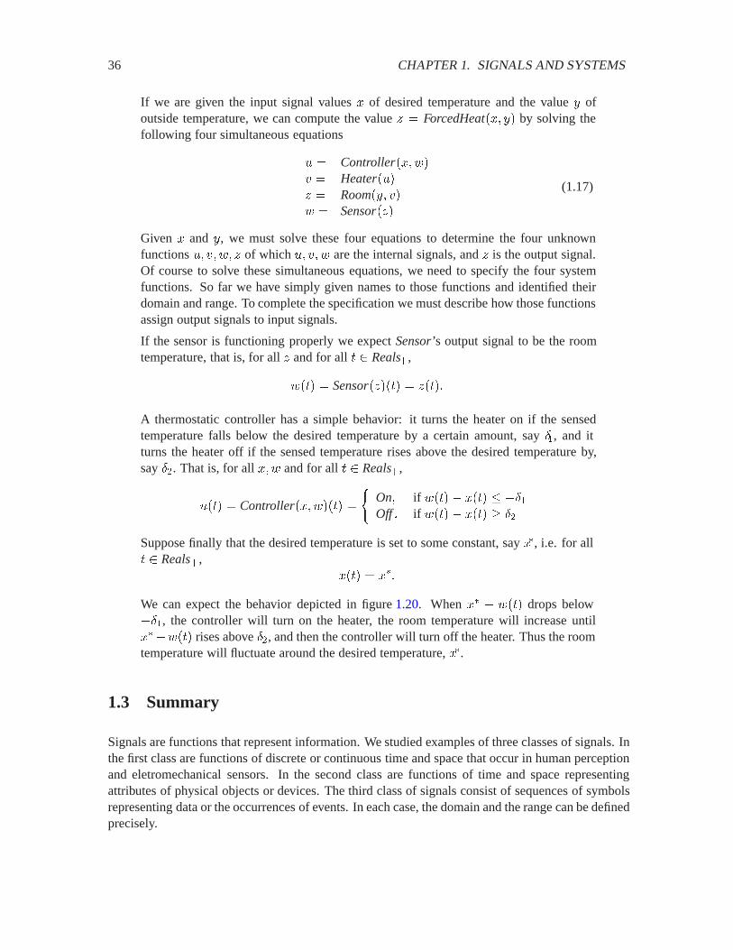
36 CHAPTER 1. SIGNALS AND SYSTEMS
If we are given the input signal values � of desired temperature and the value � ofoutside temperature, we can compute the value � � ForcedHeat��� �� by solving thefollowing four simultaneous equations
0 � Controller���/�" � Heater�0�� � Room��� "�/ � Sensor���
(1.17)
Given � and �, we must solve these four equations to determine the four unknownfunctions 0� "� /� � of which 0� "� / are the internal signals, and � is the output signal.Of course to solve these simultaneous equations, we need to specify the four systemfunctions. So far we have simply given names to those functions and identified theirdomain and range. To complete the specification we must describe how those functionsassign output signals to input signals.
If the sensor is functioning properly we expect Sensor’s output signal to be the roomtemperature, that is, for all � and for all Reals�,
/�� � Sensor����� � ����
A thermostatic controller has a simple behavior: it turns the heater on if the sensedtemperature falls below the desired temperature by a certain amount, say �, and itturns the heater off if the sensed temperature rises above the desired temperature by,say �. That is, for all ��/ and for all Reals�,
0�� � Controller���/��� �
�On� if /�� � ��� � ��Off � if /�� � ��� � �
Suppose finally that the desired temperature is set to some constant, say ��, i.e. for all Reals�,
��� � ���
We can expect the behavior depicted in figure 1.20. When �� � /�� drops below��, the controller will turn on the heater, the room temperature will increase until���/�� rises above �, and then the controller will turn off the heater. Thus the roomtemperature will fluctuate around the desired temperature, ��.
1.3 Summary
Signals are functions that represent information. We studied examples of three classes of signals. Inthe first class are functions of discrete or continuous time and space that occur in human perceptionand eletromechanical sensors. In the second class are functions of time and space representingattributes of physical objects or devices. The third class of signals consist of sequences of symbolsrepresenting data or the occurrences of events. In each case, the domain and the range can be definedprecisely.

1.3. SUMMARY 37
x* + d2
x* + d1
x*
offon
t
w
Figure 1.20: With a thermostatic controller the room temperature will fluctu-ate around the desired temperature setting, ��
Systems are functions that transform signals. We looked at telecommunication systems, where anetwork that was originally designed for carrying voice signals is used for many other kinds of sig-nals today. One way to accomplish this is to design systems such as modems that transform signalsso that they masquerade as voice-like signals. We also looked at system models for signal degra-dation and for storage of signals. We looked at systems that are primarily concerned with discreteevents and command sequences, and we examined a feedback control system. The telephone systemand the forced air heating system were both described using block diagrams as interconnections ofsimpler component systems. In all cases, systems were given as functions where the domain andthe range are function spaces, or sets of functions.
Exercises
Each problem is annotated with the letter E, T, C which stands for exercise, requires some thought,requires some conceptualization. Problems labeled E are usually mechanical, those labeled T re-quire a plan of attack, those labeled C usually have more than one defensible answer.
1. E The function � � Reals� Realsgiven by
� Reals ��� � ������ � ���
is a mathematical example of a signal in the signal space �Reals� Reals�. Give a mathemat-ical example of a signal � in each of the following signal spaces.
(a) �Integers� Reals�
(b) �Reals� Reals��
(c) ��� � � � �� � � � � �� � � ����

38 CHAPTER 1. SIGNALS AND SYSTEMS
(d) Describe a practical application for the signal space ��� � � ��� � � � ��� � � ����. That is, what might a function in this space represent?
2. C For each of the continuous-time signals below, represent the signal in the form of � �� � $and as a sketch like figure 1.1. Carefully identify the range and domain in each case.
(a) The voltage across the terminals of a car battery.
(b) The closing prices on each day of a share of a company.
(c) The position of a moving vehicle on a straight one-lane road of length 1.
(d) The simultaneous position of two moving vehicles on the same straight one-lane roadof length 1.
(e) The sound heard in both of your ears.
3. E In digital telephony, voice is sampled at a rate of 8,000 samples/second, so the samplingperiod is �� � �� -s (microseconds). What is the sampling period and the samplingfrequency of sound in a compact disc (CD)?
4. E Figure 1.4 displays the plots of two sinusoidal signals and their sum. Sketch by hand theplots of the four functions, Step�Triangle�Sum�Diff , all with domain ��� � and range Reals,defined by: � ��� �,
Triangle�� � � ���Step�� � if ) � � if � �
Sum�� � Triangle�� � Step���
Diff �� � Triangle��� Step���
5. C The following examples of spatial information can be represented as a signal in the formof � �� � $ . Specify a reasonable choice for the range and domain in each case.
(a) An image impressed on photographic paper.
(b) An image stored in computer memory.
(c) The height of points on the surface of the earth.
(d) The location of the chairs in a room.
(e) The household voltage in Europe, which has frequency 50 Hz and is 210 volts RMS.
6. C The image called Albersconsists of an eight-inch yellow square in the center of a whitetwelve-inch square background. Express Albersas a function, by choosing the domain, range,and function assignment.
7. E How many bits are there in a ��� � � pixel image in which each pixel is represented asa 16-bit word? How long would it take to download this image over a 28 Kbps voice-bandmodem, a 384 Kbps DSL modem, a 10 Mbps Ethernet local area network?
8. C Represent these examples as data or event sequences. Specify reasonable choices for therange and domain in each case.
1.3. SUMMARY 39
(a) The result of 100 tosses of a coin,
(b) The sequence of button presses inside an elevator,
(c) The sequence of main events in a soda vending machine,
(d) Your response to a motorist who is asking directions,
(e) A play-by-play account of a game of chess.
9. C Formulate the following items of information as functions. Specify reasonable choices forthe domain and range in each case.
(a) The population of U.S. cities,
(b) The white pages in a phone book (careful: the white pages may list two identical names,and may list the same phone number under two different names),
(c) The birth dates of students in class,
(d) The broadcast frequencies of AM radio stations,
(e) The broadcast frequencies of FM radio stations, (look at your radio dial, or at the webpage:
http://www.eecs.berkeley.edu/˜eal/eecs20/sidebars/radio/index.html.
10. E Use Matlab to plot the graph of the following continuous-time functions defined over��� �, and on the same plot display 11 uniformly spaced samples (0.2 seconds apart) ofthese functions. Are these samples good representations of the waveforms?
(a) � � ��� �� Reals, where for all � ��� �, ���� � ��� �������.
(b) Chirp� ��� � � Reals, where for all ��� �, Chirp�� � �������.
11. E Suppose the pendulum of figure 1.10 is rotating counter-clockwise at a speed of one revo-lution per second over the five-second interval �� ��. Sketch a plot of the resulting function:# � �� ��� ���� ��. Assume #�� � . Also specify this function mathematically. Your plotis discontinuous, but the pendulum’s motion is continuous. Explain this apparent inconsis-tency.
12. T There is a large difference between the sets � , $ , and �� � $ �. This exercise exploressome of that difference.
(a) Suppose � � ��� �� ! and $ � �� . List all the functions from � to $ , i.e. all theelements of �� � $ �. Note that part of the problem here is to figure out how to list allthe functions.
(b) If � has ' elements and $ has � elements, how many elements does �� � $ � have?
(c) Suppose
ColormapImages� �DiscreteVerticalSpace� DiscreteHorizontalSpace
� ColorMapIndexes��
Suppose the domain of each image in this set has 6,000 pixels and the range has 256values. How many distinct images are there? Give an approximate answer in the formof �. Hint: �� � � ���� ��.

40 CHAPTER 1. SIGNALS AND SYSTEMS

Chapter 2
Defining Signals and Systems
The previous chapter describes the representation of signals and systems as functions, concentratingon how to select the domain and range. This chapter is concerned with how to give more completedefinitions of these functions. In particular, we need an assignment rule, which specifies how toassign an element in the range to each element in the domain.
There are many ways to give an assignment rule. A theme of this chapter is that these differentways have complementary uses. Procedural descriptions of the assignment rule, for example, aremore convenient for synthesizing signals or constructing implementations of a system in softwareor hardware. Mathematical descriptions are more convenient for analyzing signals and systems anddetermining their properties.
In practice it is often necessary to use several descriptions of assignment rules in combination, be-cause of their complementary uses. In designing systems, a practicing engineer is often reconcilingthese diverse views to ensure, for instance, that a particular hardware device or piece of software in-deed implements a system that is specified mathematically. We begin with a discussion of functionsin general, and then specialize to signals and systems.
2.1 Defining functions
A function � �� � $ assigns to each element in � a single element in $ , as illustrated in figure2.1. This assignment can be defined by declaring the mathematical relationship between the value in� and the value in $ , by graphing or enumerating the possible assignments, by giving a procedurefor determining the value in $ given a value in � , or by composing simpler functions. We go overeach of these in more detail in this section.
Example 2.1: In section 1.1.5 we mentioned that sequences are a special kind offunction. An infinite sequence � is a function that maps the natural numbers into someset $ , as illustrated in figure 2.2. This function fully defines any infinite sequence ofelements in $ .
41

42 CHAPTER 2. DEFINING SIGNALS AND SYSTEMS
X
x1
x2
x3
x4
Y
y1
y2
y3
y4
f : X → Y
Figure 2.1: A function � �� � $ assigns to each element in � a singleelement in $ .
Naturals
1
2
3
4
Y
y1
y2
y3
y4
s : Naturals → Y
...
Figure 2.2: An infinite sequence � is a function ��Naturals � $ that assignsto each element in Naturals a single element in $ .
2.1. DEFINING FUNCTIONS 43
2.1.1 Declarative assignment
Consider the function Square�Reals� Realsgiven by
� � Reals� Square��� � ��� (2.1)
In (2.1), we have used the universal quantifier symbol ‘�’, which means ‘for all’ or ‘for every’to declare the relationship between values in the domain of the function and values in the range.Statement (2.1) is read: “for every value of � in Reals, the function Squareevaluated at � is assignedthe value ��.” The expression “Square��� � ��” in (2.1) is an assignment.1
Expression (2.1) is an instance of the following prototype for defining functions. Define � �� � $by
� � �� ���� � expression in �� (2.2)
In this prototype, � is the name of the function to be defined, such as Square, � is the domain of � ,$ is the range of � , and ‘expression in �’ specifies the value in $ assigned to ����.
The prototype (2.2) does not say how the ‘expression in �’ is to be evaluated. In the Squareexampleabove, it was specified by the algebraic expression Square��� � ��. Such a definition of a functionis said to be declarative, because it declares properties of the function without directly explaininghow to construct the function.
Example 2.2: Here are some examples of functions of complex variables.2
The magnitude of a complex number is given by abs�Complex� Reals�, whereComplexis the set of complex numbers and Reals� is the set of set of non-negative realnumbers, and
� � � �� &� Complex� abs��� ����� � ����
The complex conjugate of a number, conjugate�Complex� Complex, is given by
� � � �� &� Complex� conjugate��� � �� &��
The exponential of a complex number, ��(�Complex� Complex, is given by3
� � Complex� ��(��� ������
��
���
It is worth emphasizing that the last definition is declarative: it does not give a proce-dure for calculating the exponential function, since the sum is infinite. Such a calcula-tion would never terminate.
1See appendix A for a discussion of the use of “=” as an assignment, vs. its use as an assertion.2See appendix B for a review of complex variables.3If this notation is unfamiliar, see box on page 63.
44 CHAPTER 2. DEFINING SIGNALS AND SYSTEMS
Example 2.3: The signum function gives the sign of a real number, signum�Reals���� � ,
� � Reals� signum��� �
����� if � ) if � � if � 2
(2.3)
The right side of this assignment tabulates three expressions for three different subsetsof the domain. Below we will consider a more extreme case of this where every valuein the domain is tabulated with a value in the range.
Example 2.4: The size of a matrix, size�Matrices� Naturals�Naturals, is given by
�3 Matrices� size�3� � �'����
where ' is the number of rows of the matrix 3 , � is the number of columns of 3 ,and Matricesis the set of all matrices.
This definition relies not only on formal mathematics, but also on the English sentencethat defines ' and �. Without that sentence, the assignment would be meaningless.
2.1.2 Graphs
Consider a function � �� � $ . To each � � , � assigns the value ���� in $ . The pair ��� �����is an element of the product set � � $ . The set of all such pairs is called the graph of � , writtengraph���. Using the syntax of sets, graph��� is the subset of � � $ defined by
graph��� � ���� �� � � � and � � ����� (2.4)
or slightly more simply,graph��� � ���� ����� � � ��
The vertical bar � is read “such that,” and the expression after it is a predicate that defines the set.4
When � � Realsand $ � Reals, we can plot graph��� on a page.
Example 2.5: Consider the graph of the function Square,
graph�Square� � ���� ��� � � Reals�
which is plotted in figure 2.3. In that figure, the horizontal and vertical axes representthe domain and the range, respectively (more precisely, a subset of the domain and therange). The rectangular region enclosed by these axes represents the product of thedomain and the range (every point in that region is a member of �Reals�Reals�). Thegraph is visually rendered by placing a black dot at every point in that region that isa member of graph�Square�. The resulting picture is the familiar plot of the Squarefunction.
4See appendix A for a review of this notation.

2.1. DEFINING FUNCTIONS 45
−1 −0.8 −0.6 −0.4 −0.2 0 0.2 0.4 0.6 0.8 10
0.1
0.2
0.3
0.4
0.5
0.6
0.7
0.8
0.9
1
Figure 2.3: Graph of Square
While the graph of � �� � $ is a subset of � � $ , it is a very particular sort of subset. For eachelement � � , there is exactly one element � $ such that ��� �� graph���. In particular, therecannot be more than one such � $ , and there cannot be no such � $ . This is, in fact, what wemean when we say that � is a function.
Example 2.6: Let � � �� � and $ � ��� �. Then
��� ��� ��� ��
is the graph of a function, but��� ��� �� ��
is not, because two points � and � are assigned to the same point, 1, in the domain.Neither is
��� ���because no point in the range is assigned to the point 2 in the domain.
The graph of Square, graph�Square�, is given by the algebraic expression ��� ���. In other cases,no such algebraic expression exists. For example, Voiceis specified through its graph in figure1.1,not through an algebraic expression. Thus, graphs can be used to define functions that cannot beconveniently given by declarative assignments.
Consider again the prototype in (2.2),
� � �� ���� � expression in �
The graph of � is
graph��� � ���� �� � � $ � � � expression in ��

46 CHAPTER 2. DEFINING SIGNALS AND SYSTEMS
X
x1
x2
x3
x4
Y
y1
y2
y3
y4
Relation ⊂ X × Y
Figure 2.4: Any subset of � � $ is a relation.
Probing further: Relations
The graph of a function � �� � $ is a subset of � � $ , as defined in (2.4). Anarbitrary subset of � � $ is called a relation. A relation is a set of tuples ��� ��that pair an element � � with an element � $ , as suggested in figure2.4. Forrelations, it is common to call � the domain and $ the codomain. A function isa special kind of relation in which for every � � there is exactly one � $such that ��� �� is an element of the relation. So a particular relation � � � � $is a function if for every � � there is a �� $ such that ��� ��� �, and if inaddition ��� ��� �, then �� � ��.
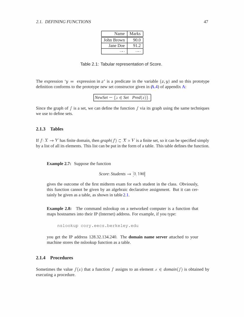
2.1. DEFINING FUNCTIONS 47
Name Marks
John Brown 90.0Jane Doe 91.2
Table 2.1: Tabular representation of Score.
The expression ‘� � expression in �’ is a predicate in the variable ��� �� and so this prototypedefinition conforms to the prototype new set constructor given in (A.4) of appendix A:
NewSet� �� Set� Pred����
Since the graph of � is a set, we can define the function � via its graph using the same techniqueswe use to define sets.
2.1.3 Tables
If � �� � $ has finite domain, then graph��� � � �$ is a finite set, so it can be specified simplyby a list of all its elements. This list can be put in the form of a table. This table defines the function.
Example 2.7: Suppose the function
Score�Students� �� �
gives the outcome of the first midterm exam for each student in the class. Obviously,this function cannot be given by an algebraic declarative assignment. But it can cer-tainly be given as a table, as shown in table 2.1.
Example 2.8: The command nslookup on a networked computer is a function thatmaps hostnames into their IP (Internet) address. For example, if you type:
nslookup cory.eecs.berkeley.edu
you get the IP address 128.32.134.240. The domain name server attached to yourmachine stores the nslookup function as a table.
2.1.4 Procedures
Sometimes the value ���� that a function � assigns to an element � domain��� is obtained byexecuting a procedure.
48 CHAPTER 2. DEFINING SIGNALS AND SYSTEMS
Example 2.9: Here is a Matlab procedure to compute the factorial function
fact� �� � � Naturals�
where Naturalsis the set of natural numbers:
fact(1) = 1;for n = 2:10
fact(n) = n * fact(n-1);end
Unlike previous mechanisms for defining a function, this one gives a constructive method to deter-mine an element in the range given an element in the domain. This style is called imperative todistinguish it from declarative. The relationship between these two styles is interesting, and quitesubtle. It is explored further in section 2.1.6.
2.1.5 Composition
Functions can be combined to define new functions. The simplest mechanism is to connect theoutput of one function to the input of another. We have been doing this informally to define systemsby connecting components in block diagrams such as figure1.18.
If the first function is �� and the second is ��, then we write the composed function as �� Æ ��. Thatis, for every � in the domain of ��,
��� Æ ������ � ����������
This is called function composition. A fundamental requirement for such a composition to bevalid is that the range of �� must be a subset of the domain of ��. In other words, any outputfrom the first function must be in the set of possible inputs for the second. Thus, for example,the output of modulator in figure 1.18 is a voice-like signal, which is precisely what the systemtelephone networkis able to accept as an input. Thus, we can compose the modulator with thetelephone network. Without this input-output connection restriction, the interconnection would bemeaningless.5
It is worth pausing to study the notation �� Æ ��. Assume ���� � $ and ����� � $ �. Then if
$ � � �, we can define�� � �� Æ ���
where ���� � $ � such that� � �� ����� � ��������� (2.5)
Notice that �� is applied first, and then ��. Why is �� listed second in �� Æ ��? This conventionsimply mirrors the ordering of ��������� in (2.5). We can visualize �� as in figure 2.5.
5We just called an element in the domain of a function its input and the corresponding value of the function its output.This interpretation of domain as inputs and range as outputs is natural, and it is the reason that systems are described byfunctions.
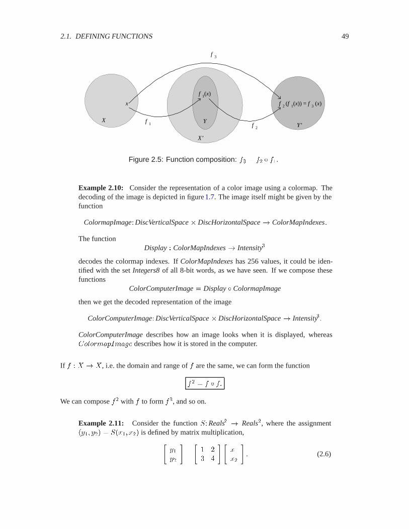
2.1. DEFINING FUNCTIONS 49
x
X
f 1(x)
Y
X’
Y’f 1 f 2
f 3
f 2 (f 1(x)) = f 3 (x)
Figure 2.5: Function composition: �� � �� Æ ��.
Example 2.10: Consider the representation of a color image using a colormap. Thedecoding of the image is depicted in figure 1.7. The image itself might be given by thefunction
ColormapImage�DiscVerticalSpace� DiscHorizontalSpace� ColorMapIndexes�
The functionDisplay � ColorMapIndexes� Intensity�
decodes the colormap indexes. If ColorMapIndexeshas 256 values, it could be iden-tified with the set Integers8of all 8-bit words, as we have seen. If we compose thesefunctions
ColorComputerImage� DisplayÆ ColormapImage
then we get the decoded representation of the image
ColorComputerImage�DiscVerticalSpace� DiscHorizontalSpace� Intensity��
ColorComputerImagedescribes how an image looks when it is displayed, whereas�4,4�'�(�'��� describes how it is stored in the computer.
If � � � � � , i.e. the domain and range of � are the same, we can form the function
�� � � Æ ��
We can compose �� with � to form ��, and so on.
Example 2.11: Consider the function .�Reals� � Reals�, where the assignment���� ��� � .���� ��� is defined by matrix multiplication,
����
��
�� �
� ����
�� (2.6)
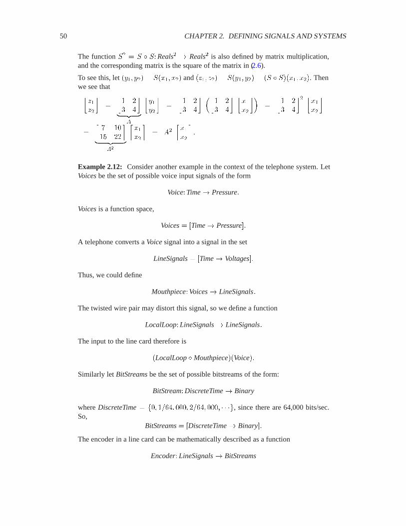
50 CHAPTER 2. DEFINING SIGNALS AND SYSTEMS
The function .� � . Æ .�Reals� � Reals� is also defined by matrix multiplication,and the corresponding matrix is the square of the matrix in (2.6).
To see this, let ���� ��� � .���� ��� and ���� ��� � .���� ��� � �. Æ .����� ���. Thenwe see that�
����
�
� �� �
� �� �
�
�����
�
� �� �
�� �� �
�����
��
� �� �
� �����
�
�� � ��
� �� �
��
�����
� ��
�����
�
Example 2.12: Consider another example in the context of the telephone system. LetVoicesbe the set of possible voice input signals of the form
Voice�Time� Pressure�
Voicesis a function space,
Voices� �Time� Pressure��
A telephone converts a Voicesignal into a signal in the set
LineSignals� �Time� Voltages��
Thus, we could define
Mouthpiece�Voices� LineSignals�
The twisted wire pair may distort this signal, so we define a function
LocalLoop�LineSignals� LineSignals�
The input to the line card therefore is
�LocalLoopÆMouthpiece��Voice��
Similarly let BitStreamsbe the set of possible bitstreams of the form:
BitStream�DiscreteTime� Binary
where DiscreteTime� �� � �� � �� �� � , since there are 64,000 bits/sec.So,
BitStreams� �DiscreteTime� Binary��
The encoder in a line card can be mathematically described as a function
Encoder�LineSignals� BitStreams
2.1. DEFINING FUNCTIONS 51
or, with more detail, as a function
Encoder� �Time� Voltages�� �DiscreteTime� Binary��
The digital telephone network itself might be modeled as a function
Network�BitStreams� BitStreams�
We can continue in this fashion until we model the entire path of a voice signal throughthe telephone network as the function composition
EarpieceÆLocalLoop�ÆDecoderÆNetworkÆEncoderÆLocalLoop�ÆMouthpiece� (2.7)
Given a complete definition of each of these functions, we would be well equipped tounderstand the degradations experienced by a voice signal in the telephone network.
2.1.6 Declarative vs. imperative
Declarative definitions of functions assert a relationship between elements in the domain and ele-ments in the range. Imperative definitions give a procedure for finding an element in the range givenone in the domain. Often, both types of specifications can be given for the same function. Howeversometimes the specifications are subtly different.
Consider the functionSquareRoot�Reals� � Reals�
defined by the statement “SquareRoot��� is the unique value of � Reals� such that �� � �.” Thisdeclarative definition of SquareRootdoes not tell us how to calculate its value at any point in itsdomain. Nevertheless, it defines SquareRootperfectly well. By contrast, an imperative definitionof SquareRootwould give us a procedure, or algorithm, for calculating SquareRoot��� for a given�. Call the result of such an algorithm ��. Since the algorithm would yield an approximation inmost cases, ��� would not be exactly equal to �. So the declarative and imperative definitions are notalways the same.
Any definition of a function following the prototype (2.2) is a declarative definition. It does not givea procedure for evaluating ‘expression in �’.
Example 2.13: As another example where declarative and imperative definitions differin subtle ways, consider the following mathematical equation:
� �������
�� (2.8)
Consider the following Java statement:
y = Math.sin(x)/x;
or an equivalent Matlab statement
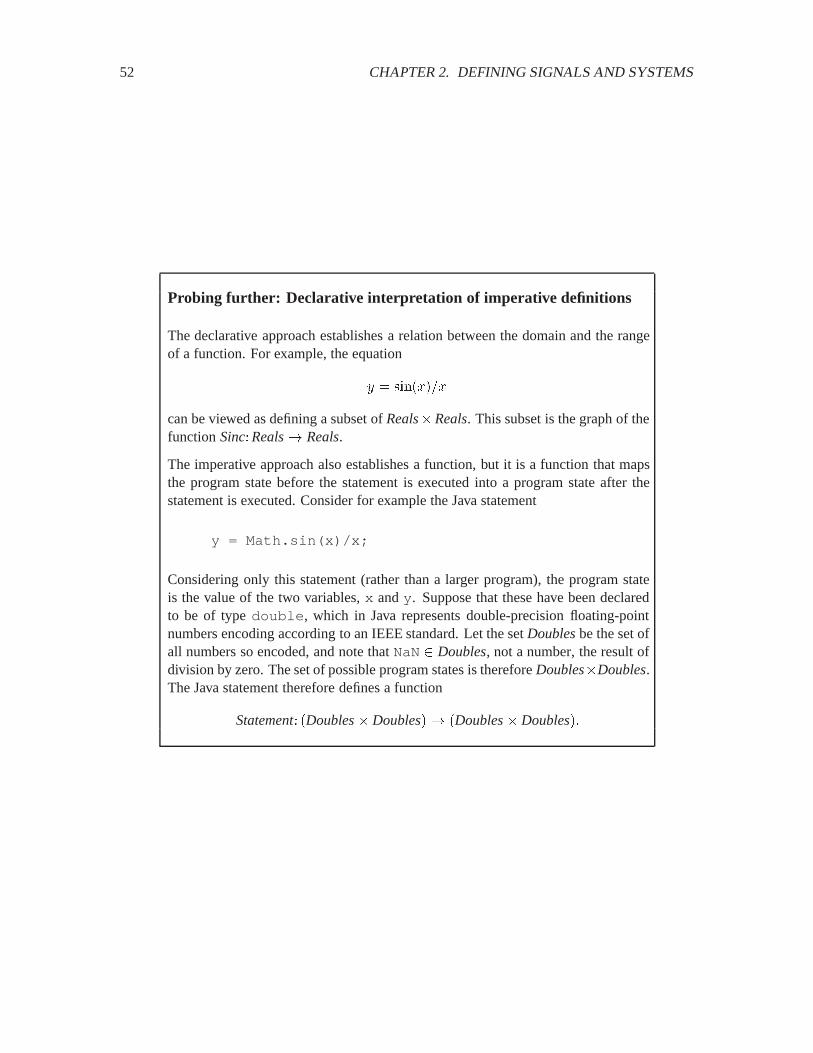
52 CHAPTER 2. DEFINING SIGNALS AND SYSTEMS
Probing further: Declarative interpretation of imperative definitions
The declarative approach establishes a relation between the domain and the rangeof a function. For example, the equation
� � ��������
can be viewed as defining a subset of Reals�Reals. This subset is the graph of thefunction Sinc�Reals� Reals.
The imperative approach also establishes a function, but it is a function that mapsthe program state before the statement is executed into a program state after thestatement is executed. Consider for example the Java statement
y = Math.sin(x)/x;
Considering only this statement (rather than a larger program), the program stateis the value of the two variables, x and y. Suppose that these have been declaredto be of type double, which in Java represents double-precision floating-pointnumbers encoding according to an IEEE standard. Let the set Doublesbe the set ofall numbers so encoded, and note that NaN Doubles, not a number, the result ofdivision by zero. The set of possible program states is therefore Doubles�Doubles.The Java statement therefore defines a function
Statement� �Doubles� Doubles�� �Doubles� Doubles��
2.1. DEFINING FUNCTIONS 53
y = sin(x)/x
Superficially, these look very similar to (2.8). There are minor differences in syntaxin the Java statement, but otherwise, it is hard to tell the difference. But there aredifferences. For one, the mathematical equation (2.8) has meaning if � is known and� is not. It declares a relationship between � and �. The Java and Matlab statementsdefine a procedure for computing y given x. Those statements have no meaning if � isknown and � is not.
The mathematical equation (2.8) can be interpreted as a predicate that defines a func-tion, for example the function Sinc�Reals� Reals, where
graph�Sinc� � ���� �� � � Reals� � � ��������� (2.9)
The Java and Matlab statements can be interpreted as imperative definitions of a func-tion6. That is, given an element in the domain, they specify how to compute an elementin the range. However, these two statements do not define the same function as in (2.9).To see this, consider the value of � when � � . Given the mathematical equation, it isnot entirely trivial to determine the value of �. You can verify that � � when � � using l’Hopital’s rule7 In contrast, the meaning of the Java and Matlab statements isthat � � � when � � , which Java and Matlab (and most modern languages) defineto be NaN, not a number8. Thus, given � � , the procedures yield different values for� than the mathematical expression.
We can see from the above example some of the strengths and weaknesses of imperative and declar-ative approaches. Given only a declarative definition, it is difficult for a computer to determinethe value of �. Symbolic mathematical software, such as Maple and Mathematica, is designed todeal with such situations, but these are very sophisticated programs. In general, using declarativedefinitions in computers requires quite a bit more sophistication than using imperative definitions.
Imperative definitions are easier for computers to work with. But the Java and Matlab statementsillustrate one weakness of the imperative approach: it is arguable that � � NaN is the wrong answer,so the Java and Matlab statements have a bug. This bug is unlikely to be detected unless, in testing,these statements happen to be executed with the value � � . A correct Java program might looklike this:
6Confusingly, many programming languages, including Matlab, use the term “function” to mean something a bitdifferent from a mathematical function. They use it to mean a procedure that can compute an element in the range ofa function given an element in its domain. Under certain restrictions (avoiding global variables for example), Matlabfunctions do in fact compute mathematical functions. But in general, they do not.
7l’Hopital’s rule states that if ���� � ���� � �, then
������
����
����� ���
���
� ����
������
if the limit exists, where � ���� is the derivative of � with respect to �, and ����� is the derivative of � with respect to �.8An exception is symbolic algebra programs, such as Mathematica or Maple, which will evaluate ������� to 1 when
� � �. These programs use sophisticated, rule-based solution techniques, and, in effect, recognize the need and applyl’Hopital’s rule.

54 CHAPTER 2. DEFINING SIGNALS AND SYSTEMS
if (x == 0.0) y = 1.0;else y = Math.sin(x)/x;
Thus, the imperative approach has the weakness that ensuring correctness is more difficult. Humanshave developed a huge arsenal of techniques and skills for thoroughly understanding declarativedefinitions (thus lending confidence in their correctness), but we are only beginning to learn how toensure correctness in imperative definitions.
2.2 Defining signals
Signals are functions. Thus, both declarative and imperative approaches can be used to define them.
2.2.1 Declarative definitions
Consider for example an audio signal �, a pure tone at 440 Hz (middle A on the piano keyboard).Recall that audio signals are functions Sound�Time � Pressure, where the set Time � Realsrepresents a range of time and the set Pressurerepresents air pressure.9 To define this function, wemight give the declarative description
� Time� ��� � ������ � ���� (2.10)
In many texts, you will see the shorthand
��� � ������ � ���
used as the definition of the function �. Using the shorthand is only acceptable when the domainof the function is well understood from the context. This shorthand can be particularly misleadingwhen considering systems, and so we will only use it sparingly. A portion of the graph of thefunction (2.10) is shown in figure 1.3.
2.2.2 Imperative definitions
We can also give an imperative description of such a signal. When thinking of signals rather thanmore abstractly of functions, there is a subtle question that arises when we attempt to construct animperative definition. Do you give the value of ��� for a particular ? Or for all in the domain?Suppose we want the latter, which seems like a more complete definition of the function. Then wehave a problem. The domain of this function may be any time interval, or all time! Suppose wejust want one second of sound. Define � to be the start of that one second. Then the domainis �� �. But there are an (uncountably) infinite number of values for in this range! No Java orMatlab program could provide the value of ��� for all these values of .
9Recall further that we normalize Pressureso that zero represents the ambient air pressure. We also use arbitraryunits, rather than a physical unit such as millibars.
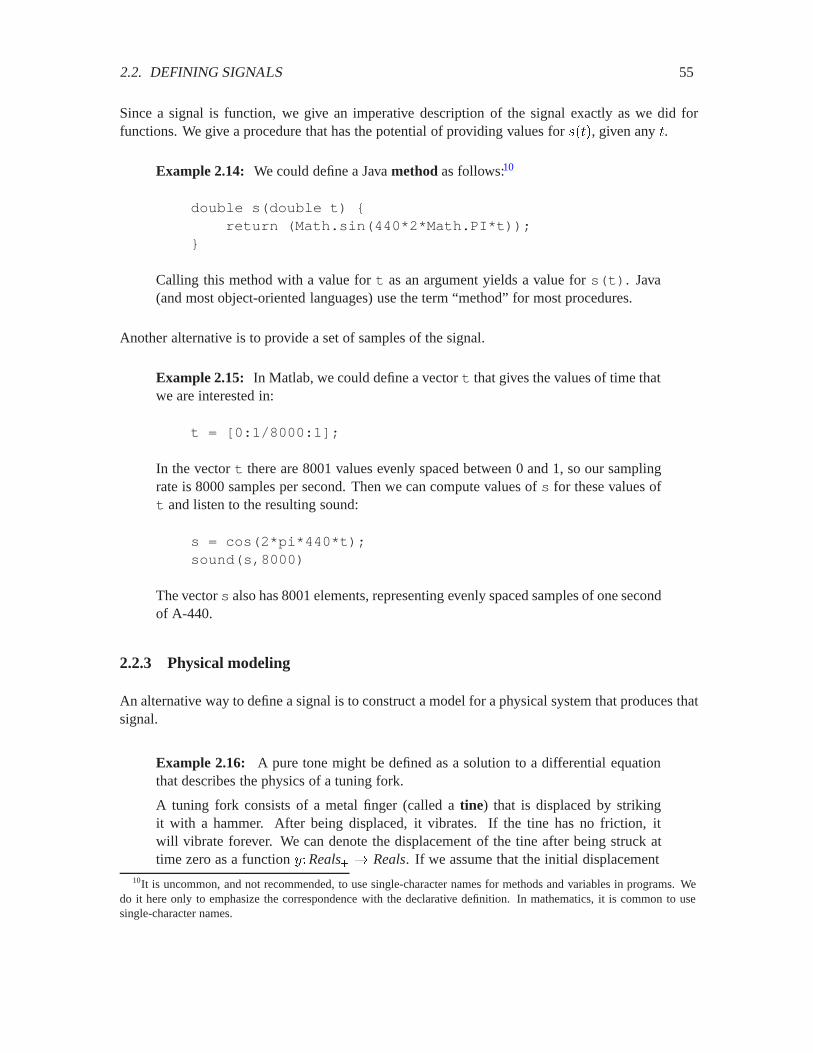
2.2. DEFINING SIGNALS 55
Since a signal is function, we give an imperative description of the signal exactly as we did forfunctions. We give a procedure that has the potential of providing values for ���, given any .
Example 2.14: We could define a Java method as follows:10
double s(double t) {return (Math.sin(440*2*Math.PI*t));
}
Calling this method with a value for t as an argument yields a value for s(t). Java(and most object-oriented languages) use the term “method” for most procedures.
Another alternative is to provide a set of samples of the signal.
Example 2.15: In Matlab, we could define a vector t that gives the values of time thatwe are interested in:
t = [0:1/8000:1];
In the vector t there are 8001 values evenly spaced between 0 and 1, so our samplingrate is 8000 samples per second. Then we can compute values of s for these values oft and listen to the resulting sound:
s = cos(2*pi*440*t);sound(s,8000)
The vector s also has 8001 elements, representing evenly spaced samples of one secondof A-440.
2.2.3 Physical modeling
An alternative way to define a signal is to construct a model for a physical system that produces thatsignal.
Example 2.16: A pure tone might be defined as a solution to a differential equationthat describes the physics of a tuning fork.
A tuning fork consists of a metal finger (called a tine) that is displaced by strikingit with a hammer. After being displaced, it vibrates. If the tine has no friction, itwill vibrate forever. We can denote the displacement of the tine after being struck attime zero as a function ��Reals� � Reals. If we assume that the initial displacement
10It is uncommon, and not recommended, to use single-character names for methods and variables in programs. Wedo it here only to emphasize the correspondence with the declarative definition. In mathematics, it is common to usesingle-character names.

56 CHAPTER 2. DEFINING SIGNALS AND SYSTEMS
displacement restorative force
tine
Figure 2.6: A tuning fork.
introduced by the hammer is one unit, then using our knowledge of physics we candetermine that for all Reals�, the displacement satisfies the differential equation
���� � ������� (2.11)
where �� is constant that depends on the mass and stiffness of the tine, and and where���� denotes the second derivative with respect to time of � (see box).
It is easy to verify that � given by
� � Reals�� ��� � ������� (2.12)
is a solution to this differential equation (just take its second derivative). Thus, thedisplacement of the tuning fork is sinusoidal. This displacement will couple directlywith air around the tuning fork, creating vibrations in the air (sound). If we choosematerials for the tuning fork so that �� � �� � ��, then the tuning fork will producethe tone of A-440 on the musical scale.
2.3 Defining systems
All of the methods that we have discussed for defining functions can be used, in principle, to definesystems. However, in practice, the situation is much more complicated for systems than for signals.Recall from section 1.2.1 that a system is a function where the domain and range are sets of signalscalled signal spaces. Elements of these domains and ranges are considerably more difficult to spec-ify than, say, an element of Realsor Integers. For this reason, it is almost never reasonable to use agraph or a table to define a system. Much of the rest of this book is devoted to giving precise waysto define systems where some analysis is possible. Here we consider some simple techniques that
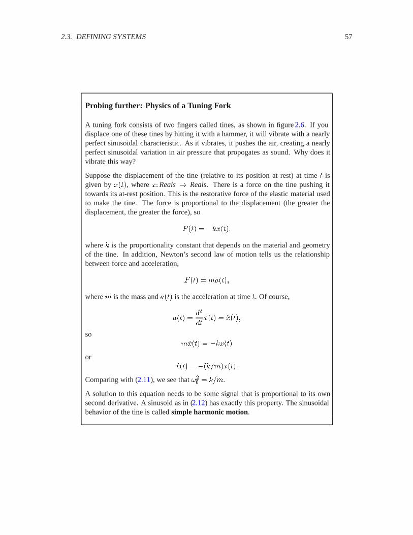
2.3. DEFINING SYSTEMS 57
Probing further: Physics of a Tuning Fork
A tuning fork consists of two fingers called tines, as shown in figure 2.6. If youdisplace one of these tines by hitting it with a hammer, it will vibrate with a nearlyperfect sinusoidal characteristic. As it vibrates, it pushes the air, creating a nearlyperfect sinusoidal variation in air pressure that propogates as sound. Why does itvibrate this way?
Suppose the displacement of the tine (relative to its position at rest) at time isgiven by ���, where ��Reals� Reals. There is a force on the tine pushing ittowards its at-rest position. This is the restorative force of the elastic material usedto make the tine. The force is proportional to the displacement (the greater thedisplacement, the greater the force), so
5 �� � �6����
where 6 is the proportionality constant that depends on the material and geometryof the tine. In addition, Newton’s second law of motion tells us the relationshipbetween force and acceleration,
5 �� � '����
where ' is the mass and ��� is the acceleration at time . Of course,
��� ���
���� � �����
so'���� � �6���
or���� � ��6�'�����
Comparing with (2.11), we see that ��� � 6�'.
A solution to this equation needs to be some signal that is proportional to its ownsecond derivative. A sinusoid as in (2.12) has exactly this property. The sinusoidalbehavior of the tine is called simple harmonic motion.
58 CHAPTER 2. DEFINING SIGNALS AND SYSTEMS
can be immediately motivated. Then we show how more complicated systems can be constructedfrom simpler ones using block diagrams. We give a rigorous meaning to these block diagrams sothat we can use them without resorting to perilous intuition to interpret them.
Consider a system . where.� �� � ��� ��� � ���� (2.13)
Suppose that � �� � �� and � � .���. Then we call the pair ��� �� a behavior of the system.A behavior is an input, output pair. The set of all behaviors is
Behaviors�.� � ���� �� � � �� � �� and � � .����
Giving the set of behaviors is one way to define a system. Explicitly giving the set Behaviors,however, is usually impractical, because it is a huge set, typically infinite (see boxes on pages520and 521). Thus, we seek other ways of talking about the relationship between a signal � and a signal� when � � .���.
To describe a system, one must specify its domain (the space of input signals), its range (the spaceof output signals), and the rule by which the system assigns an output signal to each input signal.This assignment rule is more difficult to describe and analyze than the input and output signalsthemselves. A table is almost never adequate, for example. Indeed for most systems we do nothave effective mathematical tools for describing or understanding their behavior. Thus, it is usefulto restrict our system designs to those we can understand. We first consider some simple examples.
2.3.1 Memoryless systems and systems with memory
Memoryless systems are characterized by the property that previous input values are not remem-bered when determining the current output value. More precisely, a system 5 � �Reals� $ � ��Reals� $ � is memoryless if there is a function � � $ � $ such that
� Realsand � � �Reals� $ �� �5 ������ � �������
This is illustrated in figure 2.7. In other words, at any time , the output �5 ������ depends only onthe input ��� at that same time ; in particular, it does not depend on nor on previous or futurevalues of �.
Specification of a memoryless system reduces to specification of the function � . If $ is finite, thena table may be adequate.
Example 2.17: Consider a continuous-time system with input � and output �, wherefor all Reals,
��� � �����
This example defines a simple system, where the value of the output signal at each timedepends only on the value of the input signal at that time. Such systems are said to bememoryless because you do not have to remember previous values of the input in orderto determine the current value of the output.
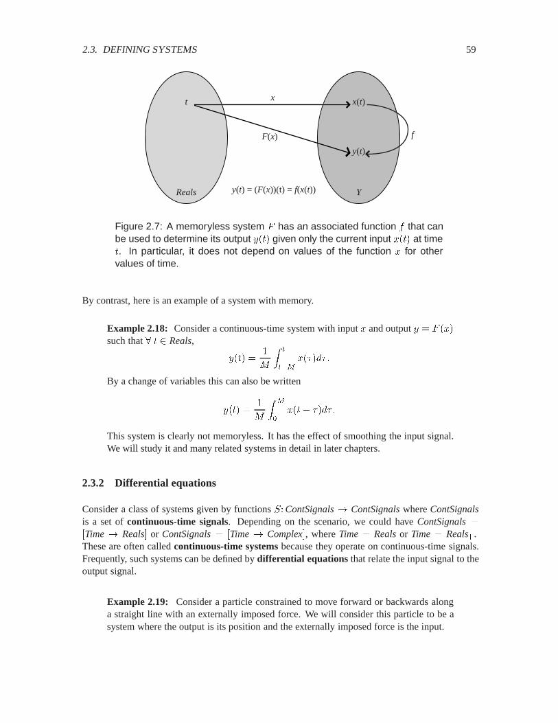
2.3. DEFINING SYSTEMS 59
Reals
t
Y
x(t)
y(t)
f
x
F(x)
y(t) = (F(x))(t) = f(x(t))
Figure 2.7: A memoryless system 5 has an associated function � that canbe used to determine its output ��� given only the current input ��� at time. In particular, it does not depend on values of the function � for othervalues of time.
By contrast, here is an example of a system with memory.
Example 2.18: Consider a continuous-time system with input � and output � � 5 ���such that � Reals,
��� �
3
� �
��������� �
By a change of variables this can also be written
��� �
3
� �
���� ���� �
This system is clearly not memoryless. It has the effect of smoothing the input signal.We will study it and many related systems in detail in later chapters.
2.3.2 Differential equations
Consider a class of systems given by functions .�ContSignals� ContSignalswhere ContSignalsis a set of continuous-time signals. Depending on the scenario, we could have ContSignals��Time� Reals� or ContSignals� �Time� Complex�, where Time� Realsor Time� Reals�.These are often called continuous-time systems because they operate on continuous-time signals.Frequently, such systems can be defined by differential equations that relate the input signal to theoutput signal.
Example 2.19: Consider a particle constrained to move forward or backwards alonga straight line with an externally imposed force. We will consider this particle to be asystem where the output is its position and the externally imposed force is the input.

60 CHAPTER 2. DEFINING SIGNALS AND SYSTEMS
Denote the position of the particle by ��Time� Reals, where Time � Reals�. Byconsidering only the non-negative reals, we are assuming that the model has a startingtime. We denote the acceleration by ��Time� Reals. By Newton’s law, which relatesforce, mass, and acceleration,
��� � '����
where ��� is the force at time , and ' is the mass. By the definition of acceleration,
� Reals�� ���� � ��� � ����'�
where ���� denotes the second derivative with respect to time of �. If we know theinitial position ��� and initial speed ���� of the particle at time 0, and if we are giventhe input force � , we can evaluate the position at any by integrating this differentialequation
��� � ��� � �����
� �
��
� �
�������'��� ���� (2.14)
We can regard the initial position and velocity as inputs, together with force, in whichcase the system is a function
Particle�Reals� Reals� �Reals� � Reals�� �Reals� � Reals��
where for any inputs ����� ����� ��, � � Particle����� ����� �� must satisfy (2.14).
Suppose for example that the input is ���� �� where ' � and � Reals�,��� � . We can calculate the position by carrying out the integration in (2.14) to findthat
� Reals�� ��� � � � ����
Suppose instead that ��� � ���� � and � Reals�, ��� � �������, where ��is some fixed number. Again, we can carry out the integration to get� �
�
� �
�������0��0 �� � ���������
����
Notice that the position of the particle is sinusoidal. Notice further that the amplitudeof this sinusoid decreases as �� increases. Intuitively, this has to be the case. If theexternally imposed force is varying more rapidly back and forth, the particle has lesstime to respond to each direction of force, and hence its excursion is less. In subsequentchapters, we will study how the response of certain kinds of systems varies with thefrequency of the input.
2.3.3 Difference equations
Consider a class of systems given by functions .�DiscSignals� DiscSignalswhere DiscSignalsisa set of discrete-time signals. Depending on the scenario, we could have DiscSignals� �Integers�Reals� or DiscSignals� �Integers� Complex�, or even DiscSignals� �Naturals� � Reals�, orDiscSignals� �Naturals� � Complex�. These are often called discrete-time systems because theyoperate on discrete-time signals. Frequently, such systems can be defined by difference equationsthat relate the input signal to the output signal.

2.3. DEFINING SYSTEMS 61
Example 2.20: Consider a system
.� �Naturals� � Reals�� �Naturals� � Reals�
where for all � �Naturals� � Reals�, .��� � � is given by
� � Integers� ���� � ����� � ���� �����
The output at each index is the average of two of the inputs. This is a simple exampleof a moving average system, where typically more than two input values get averagedto produce an output value.
Suppose that � � 0, the unit step function, defined by
� � Integers� 0��� �
� if � � otherwise
(2.15)
We can easily calculate the output �,
� � Integers� ���� �
����
if � � �� if � � otherwise
The system smoothes the transition of the unit step a bit.
A slightly more interesting input is a sinusoidal signal given by
� � Integers� ���� � ����������
The output is given by
� � Integers� ���� � ���������� � ���������� ������
By trigonometric identities,11 this can be written as
���� � � ��������� #�
where
# � ����������������
� �������������
� ��� � � ��������
As in the previous example, a sinusoidal input stimulates a sinusoidal output with thesame frequency. In this case, the amplitude of the output varies (in a fairly complicatedway) as a function of the input frequency. We will examine this phenomenon in moredetail in subsequent chapters by studying the frequency responseof such systems.
11
� ���� � � � ���� � �� � � �� � � �� � � � ���� � ��
where� � � �� � �� � � � �� � �� �
� ��
�� � �
� � �� � ���

62 CHAPTER 2. DEFINING SIGNALS AND SYSTEMS
Example 2.21: The general form for a moving average is given by12
� � �������� ���� �
3
�������
���� 6��
where � is the input and � is the output. This system is called an 3 -point movingaverage, since at any � it gives the average of the 3 most recent values of the input.It computes an average, just like example 2.18 but the integral has been replaced by itsdiscrete counterpart, the sum.
Moving averages are widely used on Wall Street to smooth out momentary fluctuations in stockprices to try to determine general trends. We will study the smoothing properties of this system. Wewill also study more general forms of difference equations of which the moving average is a specialcase.
The examples above give declarative definitions of systems. Imperative definitions require giving aprocedure for computing the output signal given the input signal. It is clear how to do that with thememoryless system, assuming that an imperative definition of the function � is available, and withthe moving average. The integral equation, however, is harder to define imperatively. An imperativedescription of such systems that is suitable for computation on a computer requires approximationvia solvers for differential equations. Simulink, for example, which is part of the Matlab package,provides such solvers. Alternatively, an imperative description can be given in terms of analogcircuits or other physical systems that operate directly on the pertinent continuous domain. Discrete-time systems often have reasonable imperative definitions as state machines, considered in detailin the next chapter.
2.3.4 Composing systems using block diagrams
We have been using block diagrams informally to describe systems. But it turns out that blockdiagrams can have as rigorous and formal a meaning as mathematical notations. We begin theexploration of this concept here, and pursue it much further in chapter4.
A block diagram is a visual syntax for describing a system as an interconnection of other (compo-nent) systems, each of which emphasizes one particular input-to-output transformation of a signal.A block diagram is a collection of blocks interconnected by arrows. Arrows are labeled by signals.Each block represents an individual system that transforms an incoming or input signal into anoutgoing or output signal. For example, modulatorin figure 1.18 is a system that transforms a bitsequence into a voice-like signal.
A block diagram, which is a composition of systems, is itself a system. We can use function com-position, as discussed in section 2.1.5, to give a precise meaning to this larger system. A blockrepresents a function, and the connection of an output from one block to the input of another repre-sents the composition of their two functions. The only requirement for interconnecting two blocksis that the output of the first block must be an acceptable input for the second. Thus, for example,
12If this notation is unfamiliar, see box on page 63.
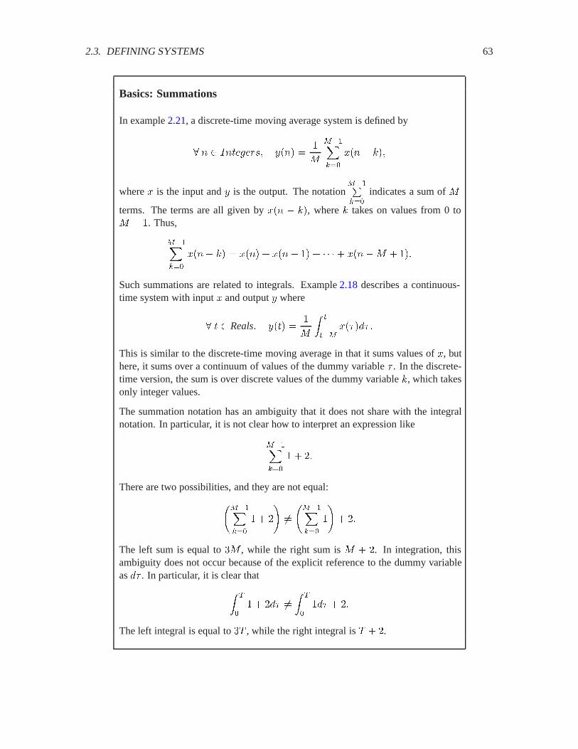
2.3. DEFINING SYSTEMS 63
Basics: Summations
In example 2.21, a discrete-time moving average system is defined by
� � �������� ���� �
3
�������
���� 6��
where � is the input and � is the output. The notation�������
indicates a sum of 3
terms. The terms are all given by ��� � 6�, where 6 takes on values from 0 to3 � . Thus,
�������
���� 6� � ���� � ���� � � � ����3 � ��
Such summations are related to integrals. Example 2.18 describes a continuous-time system with input � and output � where
� Reals� ��� �
3
� �
��������� �
This is similar to the discrete-time moving average in that it sums values of �, buthere, it sums over a continuum of values of the dummy variable � . In the discrete-time version, the sum is over discrete values of the dummy variable 6, which takesonly integer values.
The summation notation has an ambiguity that it does not share with the integralnotation. In particular, it is not clear how to interpret an expression like
�������
� ��
There are two possibilities, and they are not equal:��������
� �
�����������
�� ��
The left sum is equal to �3 , while the right sum is 3 � �. In integration, thisambiguity does not occur because of the explicit reference to the dummy variableas �� . In particular, it is clear that
� �
� � ��� ��
� �
��� � ��
The left integral is equal to � , while the right integral is � �.

64 CHAPTER 2. DEFINING SIGNALS AND SYSTEMS
S : X → Yx ∈ X y ∈Y
Y = [DY → RY]X = [DX → RX]
Figure 2.8: The simplest block diagram represents a function . that mapsan input signal � � to an output signal � $ . The domain and range ofthe input are �� and �� , repectively, and of the output, �� and �� .
the output of modulator in figure 1.18 is a voice-like signal, which is precisely what the systemtelephone networkis able to accept as an input.
Block diagrams can be much more readable than symbolic function composition, particularly forcomplicated interconnections. They also offer a natural hierarchy, where we can combine blocks tohide certain signals and component systems and to emphasize others. For instance, the telephone networkin figure 1.18 hides the details shown in figure 1.14. This emphasizes the POTS capabilities of thetelephone network, while hiding its other features.
For certain sorts of blocks, composing them in a block diagram results in a new system whoseproperties are easy to determine. In chapter 4 we will show how to combine state machine blocksto define a new state machine. In chapter 8 we will show how to combine filter blocks to define newfilter blocks. Here, we consider the composition of blocks when all we know about the blocks isthat they represent functions with a given domain and range. No further structure is available.
The simplest block diagram has a single block, as in figure 2.8. The block represents a systemwith input signal � and output signal �. Here, � denotes a variable over the set � , and � denotes avariable over the set $ . The system is described by the function .�� � $ . Both � and $ are setsof functions or signals. Therefore the variables � and � themselves denote functions.
In general, a system obtained by a cascade composition of two blocks is given by the compositionof the functions describing those blocks. In figure2.9 the function . describes the system obtainedby connecting the systems .� and .�, with . � .� Æ .�, i.e.
� � �� .��� � .��.������
The combined system has input signal �, output signal �, and internal signal �. (The internal signalis not visible in the input or output of the combined system.) Of course, the range of the first systemmust be contained by the domain of the second for this composition to make sense. In the figure,the typical case is shown where this range and domain are the same. The voice path in (2.7) is anexample of cascade composition.
Consider two more block diagrams with slightly more complicated structure. Figure2.10 is similarto figure 2.9. The system described by .� is the same as before, but the system described by .� hasa pair of input signals �/� �� 7�$ . The combined system has the pair ���/� ��7 as inputsignal, � as output signal, � as internal signal, and it is described by the function .�� �7 � % ,where
����/� � �7� .���/� � .��/�.������ (2.16)

2.3. DEFINING SYSTEMS 65
Probing further: Composition of graphs
We suggest a general method for writing down a declarative specification of theinterconnected system . in figure 2.9 in terms of the subsystems .� and .� and theconnection restriction that the output of .� be acceptable as an input of .�.
We describe .� and .� by their graphs,
graph�.�� � ���� ��� � � $ � �� � .�����
graph�.�� � ����� �� $ � % � � � .������and we specify the connection restriction as the predicate
�� � ���
We use different dummy variables �� and �� to distinguish between the two systemsand the connection restriction.
The graph of the combined system . is then given by
graph�.� � ���� �� � � % � ���������� ��� graph�.�� � ���� �� graph�.�� � �� � ���
Here, � denotes logical conjunction, “and.” It is now straightforward to show thatgraph�.� � graph�.� Æ .�� so that . � .� Æ .�.
In the case of the cascade composition of figure2.9 this elaborate method is unnec-essary, since we can write down . � .� Æ .� simply by inspecting the figure. Butfor feedback connections, we may not be able to write down the combined systemdirectly.
There are three other reasons to understand this method. First, we use it later toobtain a description of interconnected state machines from their component ma-chines. Second, this method is used to describe electronic circuits. Third, if wewant a computer to figure out the description of the interconnected system from adescription of the subsystems and the connection restrictions, we have to design analgorithm that the computer must follow. Such an algorithm can be based on thisgeneral method.
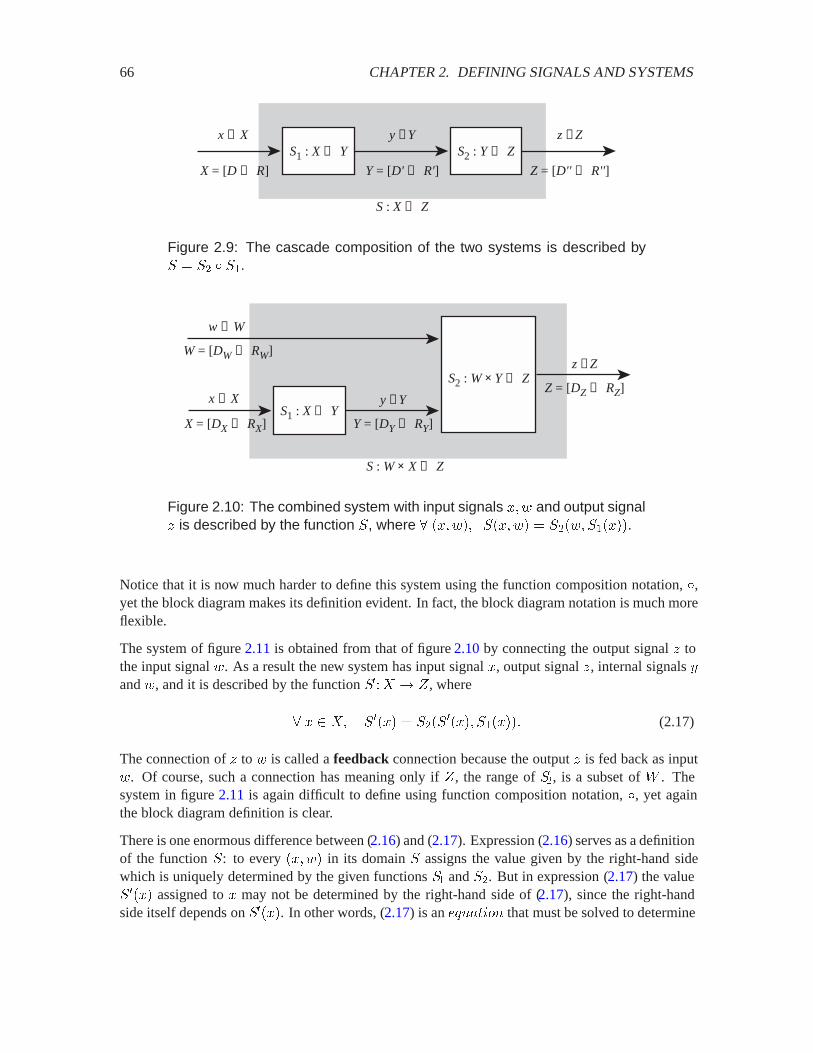
66 CHAPTER 2. DEFINING SIGNALS AND SYSTEMS
S1 : X → Yx ∈ X y ∈Y
X = [D → R] Y = [D' → R']
S2 : Y → Zz ∈Z
Z = [D'' → R'']
S : X → Z
Figure 2.9: The cascade composition of the two systems is described by. � .� Æ .�.
S1 : X → Yx ∈ X y ∈Y
S2 : W × Y → Zz ∈Z
Y = [DY → RY]X = [DX → RX]
Z = [DZ → RZ]
w ∈ W
W = [DW → RW]
S : W × X → Z
Figure 2.10: The combined system with input signals ��/ and output signal� is described by the function ., where � ���/�� .���/� � .��/�.�����.
Notice that it is now much harder to define this system using the function composition notation, Æ,yet the block diagram makes its definition evident. In fact, the block diagram notation is much moreflexible.
The system of figure 2.11 is obtained from that of figure 2.10 by connecting the output signal � tothe input signal /. As a result the new system has input signal �, output signal �, internal signals �and /, and it is described by the function .��� � % , where
� � �� .���� � .��.����� .������ (2.17)
The connection of � to / is called a feedback connection because the output � is fed back as input/. Of course, such a connection has meaning only if % , the range of .�, is a subset of 7 . Thesystem in figure 2.11 is again difficult to define using function composition notation, Æ, yet againthe block diagram definition is clear.
There is one enormous difference between (2.16) and (2.17). Expression (2.16) serves as a definitionof the function .: to every ���/� in its domain . assigns the value given by the right-hand sidewhich is uniquely determined by the given functions .� and .�. But in expression (2.17) the value.���� assigned to � may not be determined by the right-hand side of (2.17), since the right-handside itself depends on .����. In other words, (2.17) is an �80�&4� that must be solved to determine
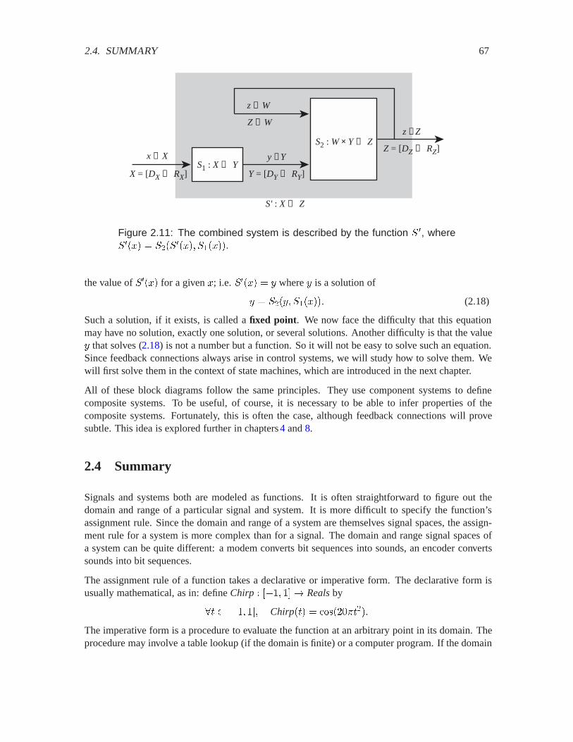
2.4. SUMMARY 67
S1 : X → Yx ∈ X y ∈Y
S2 : W × Y → Zz ∈Z
Y = [DY → RY]X = [DX → RX]
Z = [DZ → RZ]
z ∈ W
Z ⊂ W
S' : X → Z
Figure 2.11: The combined system is described by the function . �, where.���� � .��.
����� .�����.
the value of .���� for a given �; i.e. .���� � � where � is a solution of
� � .���� .������ (2.18)
Such a solution, if it exists, is called a fixed point. We now face the difficulty that this equationmay have no solution, exactly one solution, or several solutions. Another difficulty is that the value� that solves (2.18) is not a number but a function. So it will not be easy to solve such an equation.Since feedback connections always arise in control systems, we will study how to solve them. Wewill first solve them in the context of state machines, which are introduced in the next chapter.
All of these block diagrams follow the same principles. They use component systems to definecomposite systems. To be useful, of course, it is necessary to be able to infer properties of thecomposite systems. Fortunately, this is often the case, although feedback connections will provesubtle. This idea is explored further in chapters 4 and 8.
2.4 Summary
Signals and systems both are modeled as functions. It is often straightforward to figure out thedomain and range of a particular signal and system. It is more difficult to specify the function’sassignment rule. Since the domain and range of a system are themselves signal spaces, the assign-ment rule for a system is more complex than for a signal. The domain and range signal spaces ofa system can be quite different: a modem converts bit sequences into sounds, an encoder convertssounds into bit sequences.
The assignment rule of a function takes a declarative or imperative form. The declarative form isusually mathematical, as in: define Chirp � ��� �� Realsby
� ��� �� Chirp�� � ���������
The imperative form is a procedure to evaluate the function at an arbitrary point in its domain. Theprocedure may involve a table lookup (if the domain is finite) or a computer program. If the domain
68 CHAPTER 2. DEFINING SIGNALS AND SYSTEMS
is infinite, the evaluation procedure may only yield an approximation of the declarative form of the“same” function.
A physical system is often described using differential or difference equations that embody its “lawof motion.” A mechanical system’s law of motion is derived from Newton’s laws. An electricalcircuit’s law of motion is derived from Kirchhoff’s laws and the laws of the circuit’s constitutiveelements: resistors, capacitors, inductors, transistors.
Most systems are built by composing smaller subsystems. The composition may be expressed inthe visual syntax of block diagrams or, mathematically, using function composition. Feedback isthe most complex form of system composition: a feedback specification requires the solution of afixed point equation.
Exercises
Each problem is annotated with the letter E, T, C which stands for exercise, requires some thought,and requires some conceptualization. Problems labeled E are usually mechanical, those labeled Trequire a plan of attack, those labeled C usually have more than one defensible answer.
1. E The broadcast signal of an AM radio station located at 110 on your dial has a carrierfrequency of 110 kHz. An AM signal that includes the carrier has the form
� Time� AMSignal�� � � �'��� ������ � � ��
where ' is an audio signal like Voicein figure 1.1, except that � Time, �'��� ) . Sinceyou cannot easily plot such a high frequency signal, give an expression for and plot AMSignal(using Matlab) for the case where Time� �� �, '�� � ������, and the carrier frequencyis 20 Hz.
2. T This problem studies the relationship between the notion of delay and the graph of a func-tion.
(a) Consider two functions � and � from Realsinto Realswhere � Reals, ��� � and��� � �� � ��, where � is a fixed number. Sketch a plot of � and � for � � and� � �. Observe that if � 2 then graph��� is obtained by moving graph��� to theright, and if � ) by moving it to the left.
(b) Show that if � �Reals� Realsis any function whatsoever, and � � ��� � ��� ��,then if �� �� graph���, then � � �� �� graph���. This is another way of sayingthat if � 2 then the graph is moved to the right, and if � ) then the graph is movedto the left.
(c) If represents time, and if � 2 , we say that � is obtained by delaying� . Why is itreasonable to say this?
3. E Indicate whether the following statements are true or false.
(a) ��� �� � � ��� �� � �Naturals� ��� ��

2.4. SUMMARY 69
-1 0 1
1
-1 0 1
1
-0.5
graph(f )graph(g)
Figure 2.12: Graphs of two functions. The bold line is the graph.
(b) �� � � � graph��� � � �� � $ � � � $
(c) 5 � �Reals� Reals� � �Reals� Reals�, such that � Reals, and � � �Reals�Reals�,
�5 ������ � ������ ���is a memoryless system.
(d) Let � �Reals� Realsand ��Reals� Reals, where � is obtained by delaying � by� Reals. That is,
� Reals� ��� � ��� ���
Then graph��� � graph���.
4. E Figure 2.12 shows graphs of two functions � � ��� � � ��� � and �� ��� � � ��� �.For each case, define the function by giving an algebraic expression for its value at each pointin its domain. This expression will have several parts, similar to the definition of the signumfunction in (2.3). Note that ��� � for the graph on the right. Plot graph�� Æ �� andgraph�� Æ ��.
5. T Let � � ��� �� !, $ � �� �. For each of the following subsets 9 � � � $ , determinewhether 9 is the graph of a function from � to $ , and if it is, describe the function as a table.
(a) 9 � ���� �� ��� �� �!� ��(b) 9 � ���� �� ��� ��� ��� �� �!� ��(c) 9 � ���� �� ��� ��
6. C A router in the Internet is a switch with several input ports and several output ports. Apacket containing data arrives at an input port at an arbitrary time, and the switch forwardsthe packet to one of the outgoing ports. The ports of different routers are connected bytransmission links. When a packet arrives at an input port, the switch examines the packet,extracting from it a destination address �. The switch then looks up the output port in itsrouting table, which contains entries of the form ���outputPort�. It then forwards the packetto the specified output port. The Internet works by setting up the routing tables in the routers.

70 CHAPTER 2. DEFINING SIGNALS AND SYSTEMS
F : Binm → Binn
x1 ∈ Binary
xm ∈ Binary
...
y1 ∈ Binary
yn ∈ Binary
...
Figure 2.13: The logic circuit has ' binary inputs ���� � ��� and � binaryoutputs ���� � ���.
Consider a simplified router with one input port and and two output ports, named :�, :�. Let� be the set of destination addresses.
(a) Explain why the routing table can be described as a subset � � � �:�� :�.(b) Is it reasonable to constrain to be the graph of a function from � � �:�� :�? Why?
(c) Assume the signal at the input port is a sequence of packets. How would you describethe space of input signals to the router and output signals from the router?
(d) How would you describe the switch as a function from the space of input signals to thespace of output signals?
7. C For each of the following expressions, state whether it can be interpreted as an assignment,an assertion, or a predicate. More than one choice may be valid because the full context is notsupplied.
(a) � � �,
(b) � � ��,(c) � 2 �,
(d) � 2 �,
(e) � 2 � � � ) �.
8. T A logic circuit with ' binary inputs and � binary outputs is shown in figure 2.13. It isdescribed by a function 5 �� � $ where � � Binary� and $ � Binary�. (In a circuit,the signal values 1 and 0 in Binary correspond to voltage High and Low, respectively.) Howmany such distinct logic functions 5 are there?
9. E The function ; � �Reals� � Reals� � �Naturals� � Reals� given by: �� �Reals� �Reals�,
�� Naturals�� ;������ � �����
is a mathematical example of a system with input signal space �Reals� � Reals� and outputsignal space �Naturals� � Reals�. Give a mathematical example of a system ; whose
(a) input and output signal spaces both are �Naturals� � Binary�.
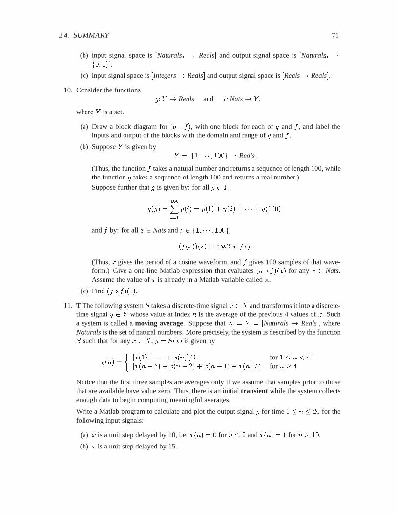
2.4. SUMMARY 71
(b) input signal space is �Naturals� � Reals� and output signal space is �Naturals� ��� �.
(c) input signal space is �Integers� Reals� and output signal space is �Reals� Reals�.
10. Consider the functions��$ � Reals and � �Nats� $�
where $ is a set.
(a) Draw a block diagram for �� Æ ��, with one block for each of � and � , and label theinputs and output of the blocks with the domain and range of � and � .
(b) Suppose $ is given by$ � ��� � � Reals�
(Thus, the function � takes a natural number and returns a sequence of length 100, whilethe function � takes a sequence of length 100 and returns a real number.)
Suppose further that � is given by: for all � $ ,
���� ��������
��&� � ��� � ���� � � ����
and � by: for all � Natsand � �� � ,
��������� � �����������
(Thus, � gives the period of a cosine waveform, and � gives 100 samples of that wave-form.) Give a one-line Matlab expression that evaluates �� Æ ����� for any � Nats.Assume the value of � is already in a Matlab variable called x.
(c) Find �� Æ ����.11. T The following system . takes a discrete-time signal � � and transforms it into a discrete-
time signal � $ whose value at index � is the average of the previous 4 values of �. Sucha system is called a moving average. Suppose that � � $ � �Naturals� Reals�, whereNaturalsis the set of natural numbers. More precisely, the system is described by the function. such that for any � � , � � .��� is given by
���� �
����� � � ������� for � � ) ������ �� � ���� �� � ���� � � ������� for � � �
Notice that the first three samples are averages only if we assume that samples prior to thosethat are available have value zero. Thus, there is an initial transient while the system collectsenough data to begin computing meaningful averages.
Write a Matlab program to calculate and plot the output signal � for time � � � � for thefollowing input signals:
(a) � is a unit step delayed by 10, i.e. ���� � for � � � and ���� � for � � .
(b) � is a unit step delayed by 15.

72 CHAPTER 2. DEFINING SIGNALS AND SYSTEMS
(c) � alternates between +1 and -1, i.e. ���� � for � odd, and ���� � � for � even.Hint: Try computing ������� for � Naturals.
(d) Comment on what this system does. Qualitatively, how is the output signal differentfrom the input signal?
12. T The following system is similar to problem 11, but time is continuous. Now � � $ ��Reals� Reals� and the system 5 �� � $ is defined as follows. For all � � and Reals
�5 ������ �
� �
�����������
Show that if � is the sinusoidal signal
� Reals ��� � �������
then � is also sinusoidal
� Reals� ��� � � ������ <��
You do not need to give precise expressions for � and <, but just show that the result hasthis form. Also, show that as � gets large, the amplitude of the output gets small. Higherfrequencies, which represent more abrupt changes in the input, are more attenuated by thesystem than lower frequencies.
Hint: The following fact from calculus may be useful:� �
���������� �
���������� ���������
Also, the identity in the footnote on page 61 might be useful to show that the output is sinu-soidal with the appropriate frequency.
13. E Suppose that � �Reals� Realsand ��Reals� Integerssuch that for all � Reals,
���� �
����
if � 2 if � � � if � )
and���� � � ��
(a) Define � � � Æ � .
(b) Suppose that
5 � �Reals� Reals� � �Reals� Reals�
9� �Reals� Reals� � �Reals� Integers�
such that for all � �Reals� Reals� and � Reals,
�5 ������� � �������
�9������� � �������
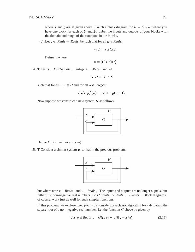
2.4. SUMMARY 73
where � and � are as given above. Sketch a block diagram for ; � 9 Æ 5 , where youhave one block for each of 9 and 5 . Label the inputs and outputs of your blocks withthe domain and range of the functions in the blocks.
(c) Let � �Reals� Reals� be such that for all � Reals,
���� � ��������
Define 0 where0 � �9 Æ 5 �����
14. T Let � � DiscSignals� �Integers� Reals� and let
9�� �� � �
such that for all �� � � and for all � Integers,
�9��� ������ � ����� ���� ��
Now suppose we construct a new system ; as follows:
G
Hx
y
Define ; (as much as you can).
15. T Consider a similar system ; to that in the previous problem,
G
Hx
y
but where now � Reals� and � Reals�. The inputs and outputs are no longer signals, butrather just non-negative real numbers. So 9�Reals� � Reals� � Reals�. Block diagrams,of course, work just as well for such simpler functions.
In this problem, we explore fixed points by considering a classic algorithm for calculating thesquare root of a non-negative real number. Let the function 9 above be given by
� �� � Reals�� 9��� �� � ���� � ����� (2.19)

74 CHAPTER 2. DEFINING SIGNALS AND SYSTEMS
(a) Show that for a given � Reals�, if the fixed point exists, then ;�Reals� � Reals�is given by
� � Reals�� ;��� ����
(b) To use the system above to calculate a square root, we simply start with a guess for �,say 1, and calculate 9��� �� repeatedly until it converges to a stable value for �. Thatstable value is the fixed point. Do this calculation for � � � and for � � �, repeatingthe evaluation of 9 until you obtain a close approximation to the true square root. Youmay want to use Matlab for this.

Chapter 3
State Machines
Systems are functions that transform signals. The domain and the range of these functions areboth signal spaces, which significantly complicates specification of the functions. A broad class ofsystems can be characterized using the concept of state and the idea that a system evolves througha sequence of changes in state, or state transitions. Such characterizations are called state-spacemodels.
A state-space model describes a system procedurally, giving a sequence of step-by-step operationsfor the evolution of a system. It shows how the input signal drives changes in state, and how theoutput signal is produced. It is thus an imperative description. Implementing a system described bya state-space model in software or hardware is straightforward. The hardware or software simplyneeds to sequentially carry out the steps given by the model. Conversely, given a piece of softwareor hardware, it is often useful to describe it using a state-space model, which yields better to analysisthan more informal descriptions.
In this chapter, we introduce state-space models by discussing systems with a finite (and relativelysmall) number of states. Such systems typically operate on event streams, often implementingcontrol logic. For example, the decision logic of modem negotiation described in chapter1 can bemodeled using a finite state model. Such a model is much more precise than the English-languagedescriptions that are commonly used for such systems.
3.1 Structure of state machines
A description of a system as a function involves three entities: the set of input signals, the set ofoutput signals, and the function itself, 5 � InputSignals� OutputSignals. For a state machine, theinput and output signals have the form
EventStream�Naturals� � Symbols�
where Naturals� � �� � �� , and Symbolsis an arbitrary set. The domain of these signalsrepresents ordering but not necessarily time (neither discrete nor continuous time). The ordering
75
76 CHAPTER 3. STATE MACHINES
of the domain means that we can say that one event occurs beforeor after another event. But wecannot say how much time elapsed between these events. In chapter5 we will study how state-spacemodels can be used with functions of time.
A state machine constructs the output signal one symbol at a time by observing the input signal onesymbol at a time. Specifically, a state machine StateMachineis a 5-tuple,
StateMachine� �States� Inputs�Outputs�update� initialState� (3.1)
where States� Inputs�Outputsare sets, updateis a function, and initialState States. The meaningof these names is:
Statesis the state space,Inputsis the input alphabet,Outputsis the output alphabet,initialState Statesis the initial state, andupdate�States� Inputs� States�Outputsis the update function.
This five-tuple is called the sets and functions model of a state machine.
Inputs and Outputsare the sets of possible input and output symbols. The set of input signalsconsists of all infinite sequences of input symbols,
InputSignals� �Naturals� � Inputs��
The set of output signals consists of all infinite sequences of output symbols,
OutputSignals� �Naturals� � Outputs��
Let � InputSignalsbe an input signal. A particular symbol in the signal can be written ���� forany � Naturals�. We write the entire input signal as a sequence
����� ���� � ����� ��
This sequence defines the function � in terms of symbols ���� Inputs, which represent particularinput symbols.
We reiterate that the index � in ���� does not refer to time, but rather to the step number. Thisis an ordering constraint only: step � occurs after step � � and before step � � . The statemachine evolves (i.e. moves from one state to the next) in steps.1
1Of course the steps could last a fixed duration of time, in which case there would be a simple relationship betweenstep number and time. The relationship may be a mixed one, where some input symbols are separated by a fixed amountof time and some are not.
3.1. STRUCTURE OF STATE MACHINES 77
3.1.1 Updates
The interpretation of updateis this. If ���� Statesis the current state at step �, and ���� Inputsis the current input symbol, then the current output symbol and the next state are given by
����� �� ����� � update������ ������
Thus the updatefunction makes it possible for the state machine to construct the output signal stepby step by observing the input signal step by step.
The state machine StateMachineof (3.1) defines a function
5 � InputSignals� OutputSignals (3.2)
such that for any input signal � InputSignalsthe corresponding output signal is � � 5 ���.However, it does much more than just define this function. It also gives us a procedure for evaluatingthis function on a particular input signal. The state response ����� ���� � and output signal �are constructed as follows:
��� � initialState� (3.3)
�� � � ����� �� ����� � update������ ������ (3.4)
Observe that if the initial state is changed, the function 5 will change, so the initial state is anessential part of the definition of a state machine.
Each evaluation of (3.4) is called a reaction because it defines how the state machine reacts to a par-ticular input symbol. Note that exactly one output symbol is produced for each input symbol. Thus,it is not necessary to have access to the entire input sequence to start producing output symbols.This feature proves extremely useful in practice, since it is usually impractical to have access to theentire input sequence (it is infinite in size!). The procedure summarized by (3.3)–(3.4) is causal, inthat the next state ����� and current output symbol ���� depend only on the initial state ��� andcurrent and past input symbols ���� ���� � ����.It is sometimes convenient to decompose updateinto two functions:
nextState�States� Inputs� Statesis the next state function,output�States� Inputs� Outputsis the output function.
The interpretation is this. If ���� is the current state, and ���� is the current input symbol at step �,the next state is
���� � � nextState������ ������
and the current output symbol is
���� � output������ ������
Evidently, for all ���� Statesand ���� Inputs,
����� �� ����� � update������ ����� � �nextState������ ������output������ ������
78 CHAPTER 3. STATE MACHINES
3.1.2 Stuttering
A state machine produces exactly one output symbol for each input symbol. For each input symbol,it may also change state (of course, it could also remain in the same state by changing back to thesame state). This means that with no input symbol, there is neither an output symbol nor a changeof state.
Later, when we compose simpler state machines to construct more complicated ones, it will proveconvenient to be explicit in the model about the fact that no input triggers no output and no statechange. We do that by insisting that the input and output symbol sets include a stuttering symbol,typically denoted absent. That is,
absent Inputs� and absent Outputs�
Moreover, we require that for any � States,
update���absent� � ���absent�� (3.5)
This is called a stuttering reaction because no progress is made. An absent input symbol triggersan absent output symbol and no state change. Now any number of absentsymbols may be insertedinto the input sequence, anywhere, without changing the non-absent output symbols. Stutteringreactions will prove essential for hybrid systems models, considered in chapter6.
Example 3.1: Consider a 60-minute parking meter. There are three (non-stuttering)input symbols: in5 and in25 which represent feeding the meter 5 and 25 cents respec-tively, and tick which represents the passage of one minute. The meter displays thetime in minutes remaining before the meter expires. When in5 occurs, this time is in-cremented by 5, and when in25 occurs it is incremented by 25, up to a maximum of60 minutes. When tick occurs, the time is decremented by 1, down to a minimum of 0.When the remaining time is 0, the display reads expired.
We can construct a finite state machine model for this parking meter. The set of statesis
States� �� � �� ���� �The input and output alphabets are
Inputs� �in5� in25� tick�absent�
Outputs� �expired� � �� ���� �absent�The initial state is
initialState� �
The update function
update�States� Inputs� States�Outputs
3.2. FINITE STATE MACHINES 79
is given by, � ���� States� ���� Inputs,
update������ ����� �
������������
��expired� if ���� � tick� ����� � � ���� � ������� � ����� � if ���� � tick� ���� 2 ��������� � �� ���������� � �� �� if ���� � in5��������� � ��� ���������� � ��� �� if ���� � in25������absent� if ���� � absent
where min is a function that returns the minimum of its arguments.
If the input sequence is �in25� tick��� in5� tick��� �, for example, then the output se-quence is2
�expired� ��� ��� ���� � �� � �� �� � �� �expired� ��
3.2 Finite state machines
Often, Statesis a finite set. In this case, the state machine is called a finite state machine, abbre-viated FSM. FSMs yield to powerful analytical techniques because, in principle, it is possible toexplore all possible sequences of states. The parking meter above is a finite state machine. Theremainder of this chapter and the next chapter will focus on finite state machines. We will returnto infinite state systems in chapter 5. Lab C.3 considers software implementation of finite statemachines.
When the number of states is small, and the input and output alphabets are finite (and small), wecan describe the state machine using a very readable and intuitive diagram called a state transitiondiagram.
Example 3.2: A verbal description of an automatic telephone answering machinemight go like this.
When a call arrives, the phone rings. If the phone is not picked up, thenon the third ring, the machine answers. It plays a pre-recorded greetingrequesting that the caller leave a message (“Hello, sorry I can’t answer yourcall right now ... Please leave a message after the beep”), then records thecaller’s message, and then automatically hangs up. If the phone is answeredbefore the third ring, the machine does nothing.
Figure 3.1 shows a state transition diagram for the state machine model of this answer-ing machine.
You can probably read the diagram in figure 3.1 without any further explanation. It is sufficientlyintuitive. Nonetheless, we will explain it precisely.
2We are using the common notation tick�� to mean a sequence of �� consecutive ticks.
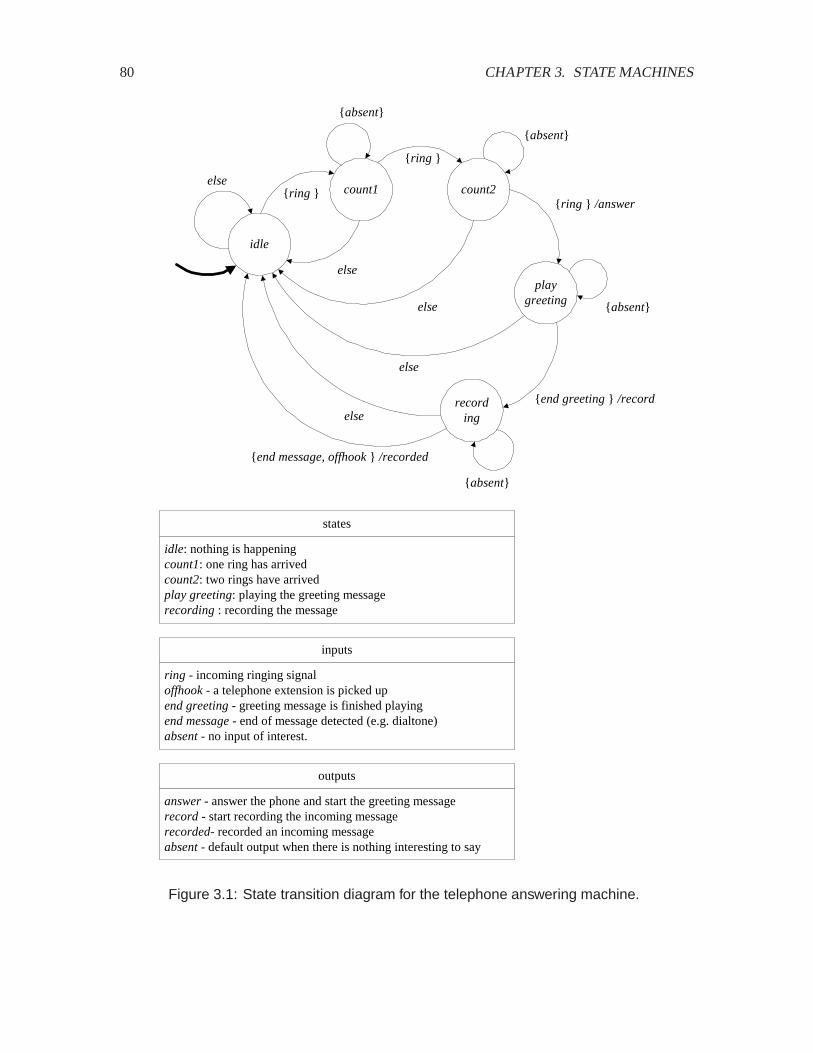
80 CHAPTER 3. STATE MACHINES
inputs
ring - incoming ringing signaloffhook- a telephone extension is picked upend greeting- greeting message is finished playingend message- end of message detected (e.g. dialtone)absent- no input of interest.
outputs
answer- answer the phone and start the greeting messagerecord- start recording the incoming messagerecorded- recorded an incoming messageabsent- default output when there is nothing interesting to say
idle
count1 count2{ring }
{ring }
{ring } /answer
else
else
playgreeting
{end greeting} /recordrecording
{end message, offhook} /recorded
else
else
else
states
idle: nothing is happeningcount1: one ring has arrivedcount2: two rings have arrivedplay greeting: playing the greeting messagerecording: recording the message
{absent}
{absent}
{absent}
{absent}
Figure 3.1: State transition diagram for the telephone answering machine.
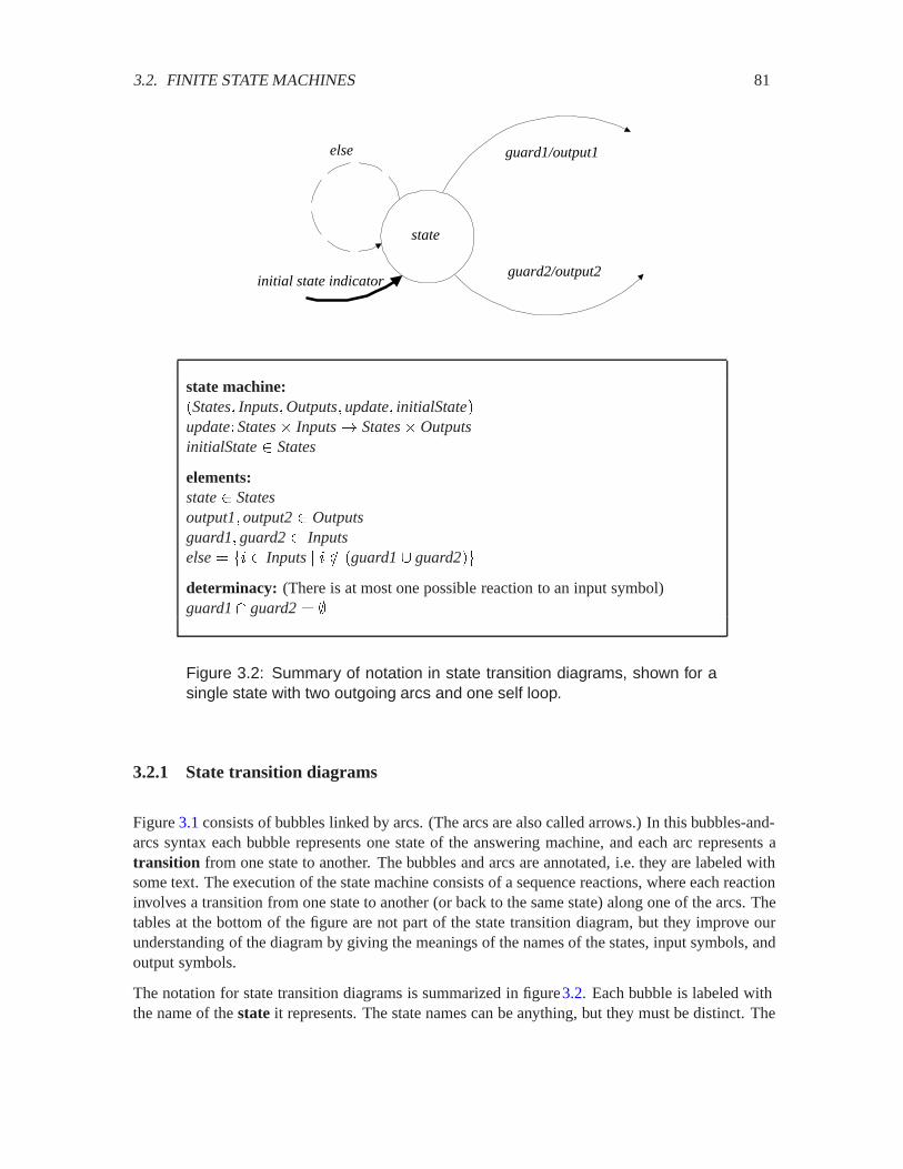
3.2. FINITE STATE MACHINES 81
state
guard1/output1
guard2/output2
else
initial state indicator
state machine:�States� Inputs�Outputs�update� initialState�update�States� Inputs� States�OutputsinitialState States
elements:state Statesoutput1�output2 Outputsguard1�guard2� Inputselse� �& Inputs� & � �guard1� guard2�determinacy: (There is at most one possible reaction to an input symbol)guard1� guard2� �
Figure 3.2: Summary of notation in state transition diagrams, shown for asingle state with two outgoing arcs and one self loop.
3.2.1 State transition diagrams
Figure 3.1 consists of bubbles linked by arcs. (The arcs are also called arrows.) In this bubbles-and-arcs syntax each bubble represents one state of the answering machine, and each arc represents atransition from one state to another. The bubbles and arcs are annotated, i.e. they are labeled withsome text. The execution of the state machine consists of a sequence reactions, where each reactioninvolves a transition from one state to another (or back to the same state) along one of the arcs. Thetables at the bottom of the figure are not part of the state transition diagram, but they improve ourunderstanding of the diagram by giving the meanings of the names of the states, input symbols, andoutput symbols.
The notation for state transition diagrams is summarized in figure3.2. Each bubble is labeled withthe name of the state it represents. The state names can be anything, but they must be distinct. The
82 CHAPTER 3. STATE MACHINES
state machine of figure 3.1 has five states. The state names define the state space,
States� �idle� count1� count2�play greeting� recording�Each arc is labeled by a guard and (optionally) an output. If an output symbol is given, it is sepa-rated from the guard by a forward slash, as in the example �ring�answergoing from state count2to play greeting. A guard specifies which input symbols might trigger the associated transition. Itis a subset of the Inputs, the input alphabet, which for the answering machine is
Inputs� �ring�offhook�end greeting�end message�absent�
In figure 3.1, some guards are labeled “else.” This special notation designates an arc that is takenwhen there is no match on any other guard emerging from a given state. The arc with the guardelseis called the else arc. Thus, elseis the set of all input symbols not included in any other guardemerging from the state. More precisely, for a given state, elseis the complement with respect toInputsof the union of the guards on emerging arcs. For example in figure3.1, for state recording,
else� �ring�offhook�end greeting�For the example in figure 3.2, elseis defined by
else� �& Inputs� & � �guard1� guard2��
If no elsearc is specified, and the set elseis not empty, then the elsearc is implicitly a self loop, asshown by the dashed arc in figure 3.2. A self loop is an arc that transitions back to the same state.When the else arc is a self loop, then the stuttering symbol may be a member of the set else.
Initially, the system of figure 3.1 is in the idle state. The initial state is indicated by the bold arc onthe left that leads into the state idle. Each time an input symbol arrives, the state machine reacts. Itchecks the guards on arcs going out of the current state and determines which of them contains theinput symbol. It then takes that transition.
Two problems might occur.
� The input symbol may not be contained in the guard of any outgoing arc. In our state machinemodels, for every state, there is at least one outgoing transition that matches the input symbol(because of the elsearc). This property is called receptiveness; it means that the machine canalways react to an input symbol. That is, there is always a transition out of the current statethat is enabled by the current input symbol. (The transition may lead back to current state ifit is a self loop.) Our state machines are said to be receptive.
� More than one guard going out from the current state may contain the input symbol. A statemachine that has such a structure is said to be nondeterministic. The machine is free tochoose any arc whose guard contains the input symbol, so more than one behavior is possiblefor the machine. Nondeterministic state machines will be discussed further below. Untilthen, we assume that the guards are always defined to give deterministic state machines.Specifically, the guards on outgoing arcs from any state are mutually exclusive. In otherwords, the intersection of any two guards on outgoing arcs of a state is empty, as indicated infigure 3.2. Of course, by the definition of the elseset, for any guard that is not else, it is truethat guard� else� �.

3.2. FINITE STATE MACHINES 83
A sequence of input symbols thus triggers a sequence of state transitions. The resulting sequence ofstates is called the state response.
Example 3.3: In figure 3.1, if the input sequence is
�ring� ring�offhook� �then the state response is
�idle� count1� count2� idle� ��The ellipsis (“ ”) are there because the answering machine generally responds to aninfinite input sequence, and we are showing only the beginning of that response. Thisbehavior can be compactly represented by a trace,
idlering�� count1
ring�� count2offhook�� idle
A trace represents the state response together with the input sequence that triggers it.This trace describes the behavior of the answering machine when someone picks up atelephone extension after two rings.3
A more elaborate trace illustrates the behavior of the answering machine when it takesa message:
idlering�� count1
ring�� count2ring�� play greeting (3.6)
end greeting�� recordingend message�� idle
A state machine also produces outputs. In figure3.1, the output alphabet is
Outputs� �answer� record� recorded�absent�An output symbol is produced as part of a reaction. The output symbol that is produced is indicatedafter a slash on an arc. If the arc annotation shows no output symbol, then the output symbol isabsent.
Example 3.4: The output sequence for the trace (3.6) is
�absent�absent�answer� record� recorded� ��There is an output symbol for every input symbol, and some of the output symbols areabsent.
It should be clear how to obtain the state response and output sequence for any input sequence. Webegin in the initial state and then follow the state transition diagram to determine the successivestate transitions for successive input symbols. Knowing the sequence of transitions, we also knowthe sequence of output symbols.
3When you lift the handset of a telephone to answer, your phone sends a signal called ‘offhook’ to the telephoneswitch. The reason for the name ‘offhook’ is that in the earliest telephone designs, the handset hung from a hook on theside of the phone. In order to answer, you had to pick the handset off the hook. When you finished your conversationyou replaced the handset on the hook, generating an ‘onhook’ signal. The onhook signal is irrelevant to the answeringmachine, so it is not included in the model.
84 CHAPTER 3. STATE MACHINES
Shorthand
State transition diagrams can get very verbose, with many arcs with complicated labels. A numberof shorthand options can make a diagram clearer by reducing the clutter.
� If no guard is specified on an arc, then that transition is always taken when the state machinereacts and is in the state from which arc emerges, as long as the input is not the stutteringsymbol. That is, giving no guard is equivalent to giving the entire set Inputsas a guard, minusthe stuttering symbol. The stuttering symbol, recall, always triggers a transition back to thesame state, and always produces a stuttering symbol on the output.
� Any clear notation for specifying subsets can be used to specify guards. For example, ifInputs� ��� �� !, then the guard ��� ! can be given by �� (read “not �”).
� An elsetransition for a state need not be given explicitly. It is an implied self-loop if it is notgiven. This is why it is shown with a dashed line in figure3.2.
� The output symbol is the stuttering symbol of Outputsif it is not given.
These shorthand notations are not always a good idea. For example, the else transitions oftencorrespond to exceptional (unexpected) input sequences, and staying in the same state might notbe the right behavior. For instance, in figure 3.1, all else transitions are shown explicitly, andall exceptional input sequences result in the machine ending up in state idle. This is probablyreasonable behavior, allowing the machine to recover. Had we left the elsetransitions implicit, wewould likely have ended up with less reasonable behavior. Use your judgment in deciding whetheror not to explicitly include elsetransitions.
3.2.2 Update table
An alternative way to describe a finite state machine is by an update table. This is simply a tabularrepresentation of the state transition diagram.
For the diagram of figure 3.1, the table is shown in figure 3.3. The first column lists the currentstate. The remaining columns list the next state and the output symbol for each of the possible inputsymbols.
The first row, for example, corresponds to the current state idle. If the input symbol is ring, the nextstate is count1and the output symbol is absent. Under any of the other input symbols, the stateremains idle and the output symbol remains absent.
Types of State Machines
The type of state machines introduced in this section are known as Mealy machines, after G. H.Mealy, who studied them in 1955. Their distinguishing feature is that output symbols are associated

3.2. FINITE STATE MACHINES 85
current (next state, output symbol) under specified input symbolstate ring offhook end greeting end message absent
idle (count1, (idle, (idle, (idle, (idle,absent) absent) absent) absent) absent)
count1 (count2, (idle, (idle, (idle, (count1,absent) absent) absent) absent) absent)
count2 (play greeting, (idle, (idle, (idle, (count2,answer) absent) absent) absent) absent)
play greeting (idle, (idle, (recording, (idle, (play greeting,absent) absent) record) absent) absent)
recording (idle, (idle, (idle, (idle, (recording,absent) recorded) absent) recorded) absent)
Figure 3.3: Update table for the telephone answering machine specifiesnext state and current output symbol as a function of current state and cur-rent input symbol.
with state transitions. That is, when a transition is taken, an output symbol is produced. Alterna-tively, we could have associated output symbols with states, resulting in a model known as Mooremachines, after F. Moore, who studied them in 1956. In a Moore machine, an output symbol isproduced while the machine is in a particular state. Mealy machines turn out to be more usefulwhen they are composed synchronously, as we will do in the next chapter. This is the reason thatwe choose this variant of the model.
It is important to realize that state machine models, like most models, are not unique. A great dealof engineering judgment goes into a picture like figure3.1, and two engineers might come up withvery different pictures for what they believe to be the same system. Often, the differences are inthe amount of detail shown. One picture may show the operation of a system in more detail thananother. The less detailed picture is called an abstraction of the more detailed picture. Also likelyare differences in the names chosen for states, input symbols and output symbols, and even in themeaning of the input and output symbols. There may be differences in how the machine respondsto exceptional circumstances (input sequences that are not expected). For example, what shouldthe answering machine do if it gets the input sequence �ring�end greeting�end message�? Thisprobably reflects a malfunction in the system. In figure 3.1, the reaction to this sequence is easy tosee: the machine ends up in the idle state.
Given these likely differences, it becomes important to be able to talk about abstraction relationsand equivalence relations between state machine models. This turns out to be a fairly sophisticatedtopic, one that we touch upon below in section 3.3.
86 CHAPTER 3. STATE MACHINES
The meaning of state
We have three equivalent ways of describing a state machine: sets and functions, the state transitiondiagram, and the update table. These descriptions have complementary uses. The table makes obvi-ous the sparsity of output symbols in the answering machine example. The table and the diagramsare both useful for a human studying the system to follow its behavior in different circumstances.The sets and functions and the table are useful for building the state machine in hardware or soft-ware. The sets and functions description is also useful for mathematical analysis.
Of course, the tables and the transition diagram can be used only if there are finitely many statesand finitely many input and output symbols, i.e. if the sets States� Inputs� ���Outputsare finite. Thesets and functions description is often equally comfortable with finite and infinite state spaces. Wewill discuss infinite-state systems in chapter 5.
Like any state machine, the telephone answering machine is a state-determined system. Once weknow its current state, we can tell what its future behavior is for any future input symbols. We donot need to know what input symbols in the past led to the current state in order to predict how thesystem will behave in the future. In this sense we can say the current state of the system summarizesthe past history of the system. This is, in fact, the key intuitive notion of state.
The number of states equals the number of patterns we need to summarize the past history. If this isintrinsically finite, then a finite-state model exists for the system. If it is intrinsically infinite, thenno finite-state model exists. We can often determine which of these two situations applies usingsimple intuition. We can also show that a system has a finite-state model by finding one. Showingthat a system does not have a finite-state model is a bit more challenging.
Example 3.5: Consider the example of a system called CodeRecognizerwhose inputand output signals are sequences of 0 and 1 (with arbitrarily inserted stuttering symbols,which have no effect). The system outputs recognizeat the end of every subsequence1100 in the input, and otherwise it outputs absent. If the input � is given by a sequence
����� ���� ��
and the output � is given by the sequence
����� ���� ��
then, if none of the input symbols is absent,
���� �
�recognize if ����� ��� ���� ��� ��� � �� ����� � �� � � �absent otherwise
(3.7)
Intuitively, in order to determine ����, it is enough to know whether the previous patternof (non-absent) inputs is 0, 1, 11, or 110. If this intuition is correct, we can implementCodeRecognizerby a state machine with four states that remember the patterns 0, 1,11, 110. The machine of figure 3.4 does the job. The fact that we have a finite-statemachine model of this system shows that this is a finite-state system.
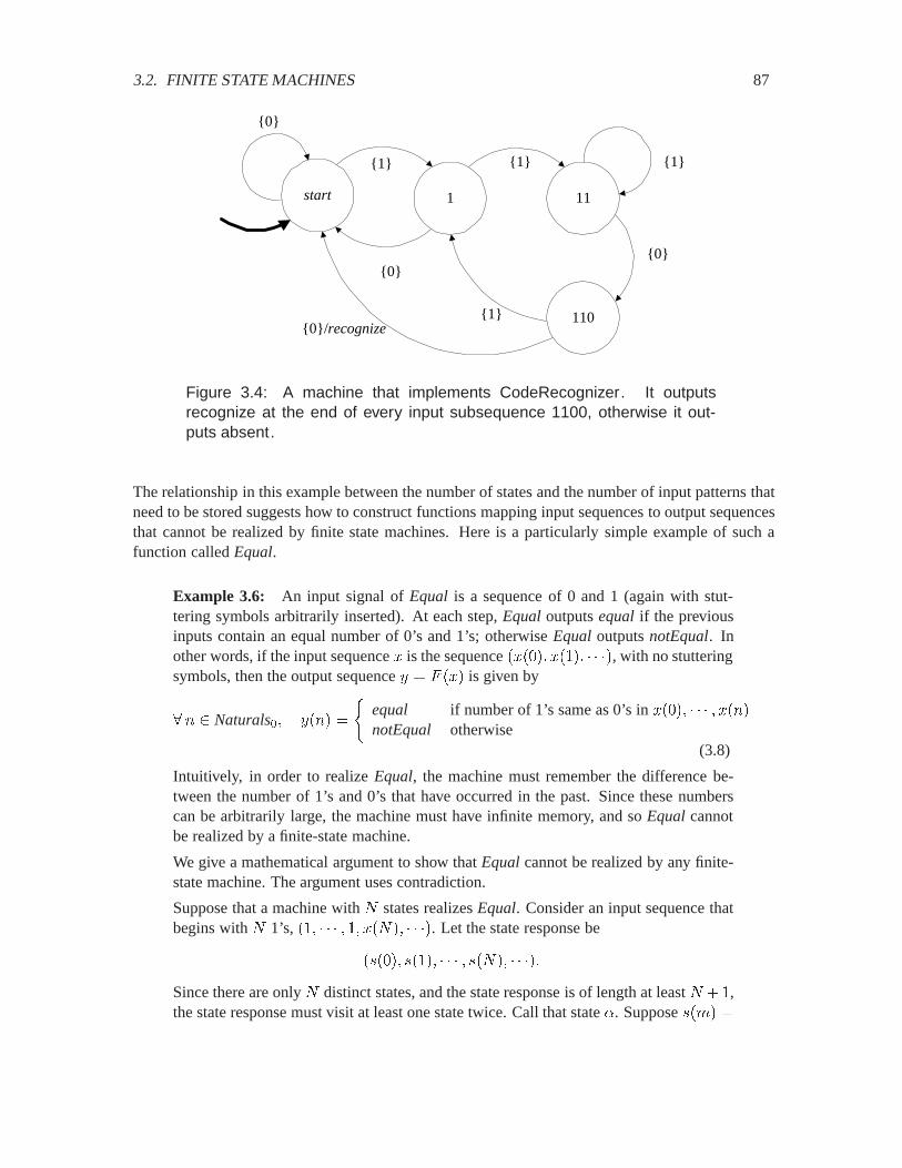
3.2. FINITE STATE MACHINES 87
start 1 11
{1} {1}
{0}{0}
110{0}/recognize
{1}
{0}
{1}
Figure 3.4: A machine that implements CodeRecognizer. It outputsrecognize at the end of every input subsequence 1100, otherwise it out-puts absent.
The relationship in this example between the number of states and the number of input patterns thatneed to be stored suggests how to construct functions mapping input sequences to output sequencesthat cannot be realized by finite state machines. Here is a particularly simple example of such afunction called Equal.
Example 3.6: An input signal of Equal is a sequence of 0 and 1 (again with stut-tering symbols arbitrarily inserted). At each step, Equal outputs equal if the previousinputs contain an equal number of 0’s and 1’s; otherwise Equal outputs notEqual. Inother words, if the input sequence � is the sequence ����� ���� �, with no stutteringsymbols, then the output sequence � � 5 ��� is given by
� � Naturals�� ���� �
�equal if number of 1’s same as 0’s in ���� � ����notEqual otherwise
(3.8)
Intuitively, in order to realize Equal, the machine must remember the difference be-tween the number of 1’s and 0’s that have occurred in the past. Since these numberscan be arbitrarily large, the machine must have infinite memory, and so Equal cannotbe realized by a finite-state machine.
We give a mathematical argument to show that Equalcannot be realized by any finite-state machine. The argument uses contradiction.
Suppose that a machine with � states realizes Equal. Consider an input sequence thatbegins with � 1’s, �� � � ����� �. Let the state response be
����� ���� � ����� ��Since there are only � distinct states, and the state response is of length at least � �,the state response must visit at least one state twice. Call that state *. Suppose ��'� �
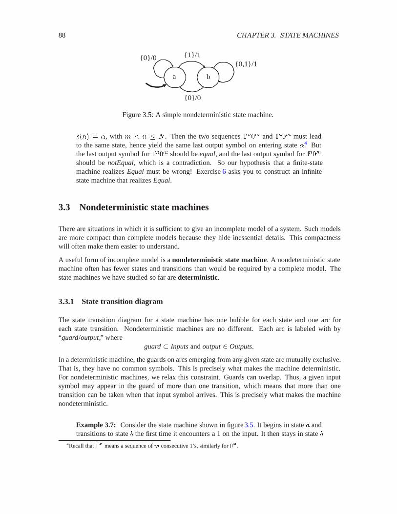
88 CHAPTER 3. STATE MACHINES
a b
{1}/1
{0}/0
{0,1}/1{0}/0
Figure 3.5: A simple nondeterministic state machine.
���� � *, with ' ) � � � . Then the two sequences �� and �� must leadto the same state, hence yield the same last output symbol on entering state *.4 Butthe last output symbol for �� should be equal, and the last output symbol for ��
should be notEqual, which is a contradiction. So our hypothesis that a finite-statemachine realizes Equal must be wrong! Exercise 6 asks you to construct an infinitestate machine that realizes Equal.
3.3 Nondeterministic state machines
There are situations in which it is sufficient to give an incomplete model of a system. Such modelsare more compact than complete models because they hide inessential details. This compactnesswill often make them easier to understand.
A useful form of incomplete model is a nondeterministic state machine. A nondeterministic statemachine often has fewer states and transitions than would be required by a complete model. Thestate machines we have studied so far are deterministic.
3.3.1 State transition diagram
The state transition diagram for a state machine has one bubble for each state and one arc foreach state transition. Nondeterministic machines are no different. Each arc is labeled with by“guard/output,” where
guard� Inputsand output Outputs�
In a deterministic machine, the guards on arcs emerging from any given state are mutually exclusive.That is, they have no common symbols. This is precisely what makes the machine deterministic.For nondeterministic machines, we relax this constraint. Guards can overlap. Thus, a given inputsymbol may appear in the guard of more than one transition, which means that more than onetransition can be taken when that input symbol arrives. This is precisely what makes the machinenondeterministic.
Example 3.7: Consider the state machine shown in figure 3.5. It begins in state � andtransitions to state � the first time it encounters a 1 on the input. It then stays in state �
4Recall that �� means a sequence of � consecutive 1’s, similarly for ��.

3.3. NONDETERMINISTIC STATE MACHINES 89
arbitrarily long. If it receives a 1 at the input, it must stay in state �. If it receives a 0,then it can either stay in � or transition to �. Given the input sequence
�� � � � � � �
then the following are all possible state responses and output sequences:
��� �� �� �� �� �� �� ��� � � � � � �
��� �� �� �� �� �� �� ��� � � � � � �
��� �� �� �� �� �� �� ��� � � � � � �
��� �� �� �� �� �� �� ��� � � � � � �
Nondeterminism can be used to construct an abstraction of a complicated machine, which is asimpler machine that has all the behaviors of the more complicated machine.
Example 3.8: Consider again the 60-minute parking meter. Its input alphabet is
Inputs� �coin5� coin25� tick�absent�
Upon arrival of coin5, the parking meter increments its count by five, up to a maximumof 60 minutes. Upon arrival of coin25, it increments its count by 25, again up to a max-imum of 60. Upon arrival of tick, it decrements its count by one, down to a minimumof zero.
A deterministic state machine model is illustrated schematically in figure3.6(a). Thestate space is
States� �� � � �which is too many states to draw conveniently. Thus, patterns in the state space aresuggested with ellipsis “ ”.
Suppose that we are interested in modeling the interaction between this parking meterand a police officer. The police officer does not care what state the parking meter isin, except to determine whether the meter has expired or not. Thus, we need only twononstuttering output symbols, so
Outputs� �safe�expired�absent�
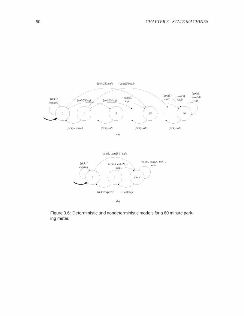
90 CHAPTER 3. STATE MACHINES
0 1
{coin5}/safe
{tick}/expired
5
{tick}/expired
{tick}/safe
...
{coin5}/safe
... 25
{tick}/safe
{coin25}/safe {coin25}/safe
60
{tick}/safe
...
{coin5,coin25}/
safe{coin5}/
safe
{coin25}/safe
{coin5}/safe
0
{tick}/expired
1
{tick}/expired
more
{tick}/safe
{coin5, coin25} / safe
{coin5, coin25} /safe
{coin5, coin25, tick} /safe
(a)
(b)
Figure 3.6: Deterministic and nondeterministic models for a 60 minute park-ing meter.

3.3. NONDETERMINISTIC STATE MACHINES 91
The symbol expiredis produced whenever the machine enters state 0.
The model has enough states that a full state transition diagram is tedious and complexenough that it might not be useful for generating insight about the design. Moreover,the detail that is modeled may not add insight about the interaction with a police officer.
Figure 3.6(b) is a nondeterministic model of the same parking meter. It has three states,
States� �� �more�
The input symbols coin5and coin25in state 0 or 1 cause a transition to state more. Theinput symbol tick in state morenondeterministically moves the state to 1 or leaves it inmore.
The top state machine has more detail than the bottom machine. Shortly, we will givea precise meaning to the phrase ‘has more detail’ using the concept of simulation. Forthe moment, note that the bottom machine can generate any output sequence that thetop machine generates, for the same input sequence. But the bottom machine can alsogenerate output sequences that the top machine cannot. For example, the sequence
�expired� safe� safe�expired� ��
in which there are two safeoutput symbols between two expiredoutput symbols is nota possible output sequence of the top machine, but it is a possible output sequence ofthe bottom machine. In the top machine, successive expiredoutput symbols must beseparated by 0 or at least five safeoutput symbols. This detail is not captured by thebottom machine. But in modeling the interaction with a police officer, this detail maynot be important, so omitting it may be entirely appropriate.
The machines that we design and build, including parking meters, are usually deterministic. How-ever, the state space of these machines is often very large, much larger than in this example, andit can be difficult to understand their behavior. We use simpler nondeterministic machine modelsthat hide inessential details of the deterministic machine. The analysis of the simpler model revealssome properties, but not all properties, of the more complex machine. The art, of course, is inchoosing the model that reveals the properties of interest.
3.3.2 Sets and functions model
The state machines we have been studying, with definitions of the form (3.1), are deterministic. Ifwe know the initial state and the input sequence, then the entire state trajectory and output sequencecan be determined. This is because any current state ���� and current input symbol ���� uniquelydetermine the next state and output symbol ����� �� ����� � update������ �����.
In a nondeterministic state machine, the next state is not completely determined by the current stateand input symbol. For a given current state ���� and input symbol ����, there may be more than onenext state. So we cannot characterize the machine by the function update������ ����� because thereis no single next state. Instead, we define a function possibleUpdatesso that possibleUpdates������ �����
92 CHAPTER 3. STATE MACHINES
is the setof possible next states and output symbols. Whereas a deterministic machine has updatefunction
update�States� Inputs� States�Outputs�
a nondeterministic machine has a (nondeterministic) state transition function
possibleUpdates�States� Inputs� � �States�Outputs�� (3.9)
where � �State�Outputs� is the power set of States�Outputs. Recall that the power set is the setof all subsets. That is, any subset of States�Outputsis an element of � �States�Outputs�.
In order for a nondeterministic machine to be receptive, it is necessary that
� ���� States� ���� Inputs possibleUpdates������ ����� �� ��Recall that a receptive machine accepts any input symbol in any state, makes a state transition(possibly back to the same state), and produces an output symbol. That is, there is no situationwhere the reaction to an input symbol is not defined.
Operationally, a nondeterministic machine arbitrarily selects the next state and current output sym-bol from possibleUpdatesgiven the current state and current input symbol. The model says nothingabout how the selection is made.
Similar to deterministic machines, we can collect the specification of a nondeterministic state ma-chine into a 5-tuple
StateMachine� �States� Inputs�Outputs�possibleUpdates� initialState�� (3.10)
The possibleUpdatesfunction is different from the updatefunction of a deterministic machine.
Deterministic state machines of the form (3.1) are a special case of nondeterministic machines inwhich possibleUpdates������ ����� consists of a single element, namely update������ �����. Inother words,
possibleUpdates������ ����� � �update������ ������Thus, any deterministic machine, as well as any nondeterministic machine, can be given by (3.10).
In the nondeterministic machine of (3.10), a single input sequence may give rise to many state re-sponses and output sequences. If ����� ���� ����� � is an input sequence, then ����� ���� ����� �is a (possible) state trajectory and ����� ���� ����� � is a (possible) output sequence providedthat
��� � initialState
�� � � ����� �� ����� possibleUpdates������ ������
A deterministic machine defines a function from an input sequence to an output sequence,
5 � InputSignals� OutputSignals�
whereInputSignals� �Naturals� � Inputs��
3.4. SIMULATION AND BISIMULATION 93
and
OutputSignals� �Naturals� � Outputs��
We define a behavior of the machine to be a pair ��� �� such that � � 5 ���, i.e., a behavior is apossible input, output pair. A deterministic machine is such that for each � InputSignals, there isexactly one � OutputSignalssuch that ��� �� is a behavior.
We define the set
Behaviors� InputSignals�OutputSignals� (3.11)
where
Behaviors�
���� �� InputSignals�OutputSignals� � is a possible output sequence for input sequence ��
For a deterministic state machine, the set Behaviorsis the graph of the function 5 .
For a nondeterministic machine, for a given � InputSignals, there may be more than one � OutputSignalssuch that ��� �� is a behavior. The set Behaviors, therefore, is no longer the graphof a function. Instead, it defines a relation—a generalization of a function where there can betwo or more distinct elements in the range corresponding to the same element in the domain. Theinterpretation is still straightforward, however: if ��� �� Behaviors, then input sequence � mayproduce output sequence �.
3.4 Simulation and bisimulation
Two different state machines with the same input and output alphabets may be equivalent in thesense that for the same input sequence, they produce the same output sequence. We explore thisconcept of equivalence in this section.
Example 3.9: The three state machines in figure 3.7, have the same input and outputalphabets:
Inputs� ��absent and Outputs� �� �absent�Machine (a) has the most states. However, its behavior is identical to that of (b). Bothmachines produce an alternating sequence of two 1’s and one 0 as they receive a se-quence of 1’s at the input. The machine in (c) is non-deterministic. It has more behav-iors than (a) or (b): it can produce any alternating sequence of at least two 1’s and onezero. Thus (c) is more general, or more abstract than the machines (a) or (b).
To study the relationships between the machines in figure3.7 we introduce the concepts of simula-tion and bisimulation. The machine in (c) is said to simulate (b) and (a). The machine in (b) is saidto bisimulate (a), or to be bisimilar to (a). Bisimulation can be viewed as a form of equivalencebetween state machines. Simulation can be viewed as a form of abstraction of state machines.
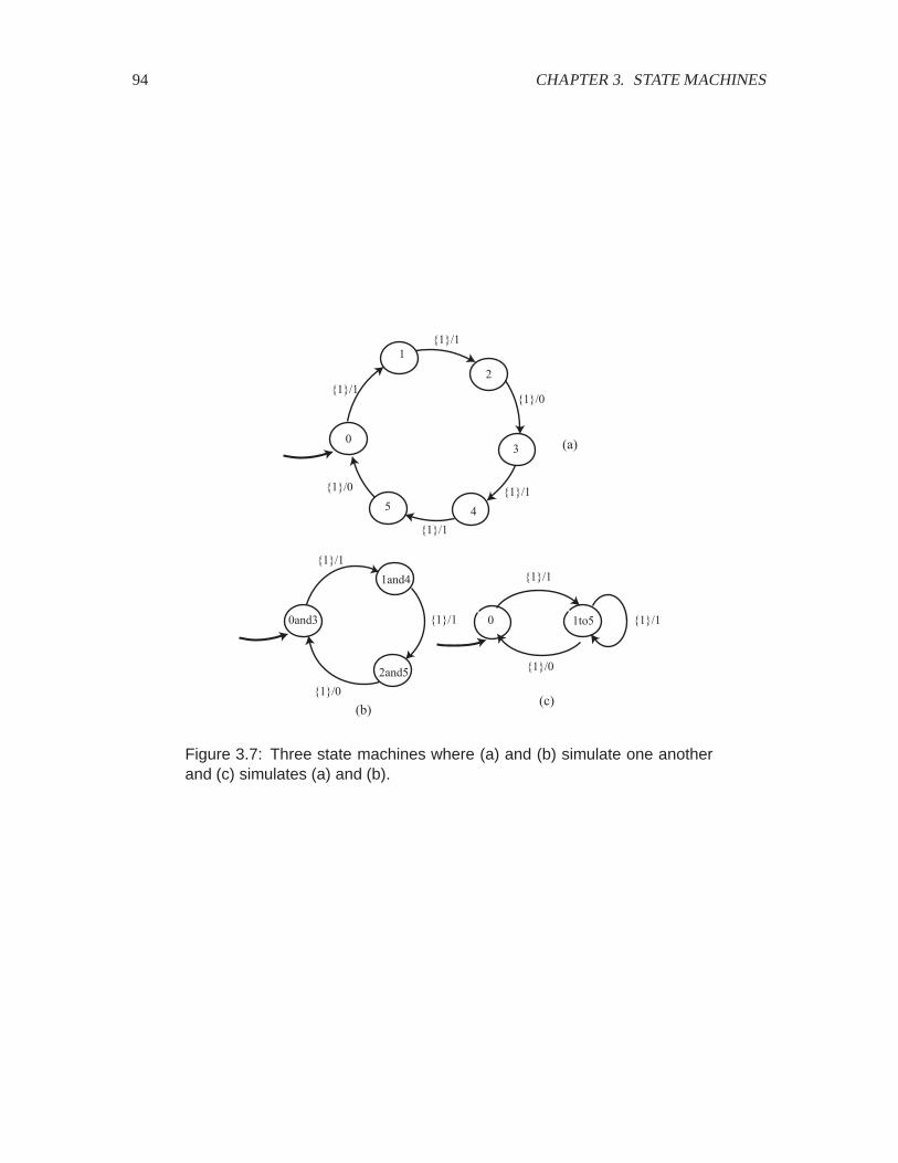
94 CHAPTER 3. STATE MACHINES
{1}/1
{1}/1
{1}/0
{1}/1
{1}/1
{1}/0
0
1
2
3
45
0and3
1and4
2and5{1}/0
{1}/1
{1}/1
{1}/1
{1}/0
{1}/10 1to5
(a)
(b)(c)
Figure 3.7: Three state machines where (a) and (b) simulate one anotherand (c) simulates (a) and (b).
3.4. SIMULATION AND BISIMULATION 95
Example 3.10: In figure 3.6, the bottom machine can generate any output sequencethat the top machine generates, for the same input sequence. The reverse is not true;there are output sequences that the bottom machine can generate that the top machinecannot. The bottom machine is an abstraction of the top one.
We will see that the bottom machine simulates the top machine (but not vice versa).
To understand simulation, it is easiest to consider a matching game between one machine andthe other, more abstract machine that simulates the first. The game starts with both machines intheir initial states. The first machine is allowed to react to an input symbol. If this machine isnondeterministic, it may have more than one possible reaction; it is permitted to choose any oneof these reactions. The second, more abstract machine must react to the same input symbol suchthat it produces the same output symbol. If it is non-deterministic, it is free to pick from among thepossible reactions any one that matches the output symbol of the first machine and that will permitit to continue to match the output symbols of the first machine in future reactions. The secondmachine “wins” this matching game if it can always match the output symbol of the first machine.We then say that the second machine simulates the first one. If the first machine can produce anoutput symbol that the second one cannot match, then the second machine does not simulate thefirst machine.
Example 3.11: We wish to determine whether (c) simulates (b) in figure 3.7. Thegame starts with the two machines in their initial states, which we jointly denote by thepair
�� � �0and3�0� States� � States��
Machine (b) (the one being simulated) moves first. Given an input symbol, it reacts. Ifit is nondeterministic, then it is free to react in any way possible, although in this case,(b) is deterministic, so it will have only one possible reaction. Machine (c) then has tomatch the move taken by (b); given the same input symbol, it must react such that itproduces the same output symbol.
There are two possible input symbols to machine (b), 1 and absent. If the input symbolis absent, the machine reacts by stuttering. Machine (c) can match this by stutteringas well. For this example, it will always do to match stuttering moves, so we will notconsider them further.
Excluding the stuttering input symbol, there is only one possible input symbol to ma-chine (b), 1. The machine reacts by producing the output symbol 1 and changing tostate 1and4. Machine (c) can match this by taking the only possible transition out ofits current state, and also produce output symbol 1. The resulting states of the twomachines are denoted
�� � �1and4�1to5� States� � States��
From here, again there is only one non-stuttering input symbol possible, so (b) reactsby moving to 2and5and producing the output symbol 1. Now (c) has two choices,
96 CHAPTER 3. STATE MACHINES
but in order to match (b), it chooses the (self-loop) transition which produces 1. Theresulting states are
�� � �2and5�1to5� States� � States��
From here, (b) reacts to the non-stuttering input symbol by moving to 0and3and pro-ducing output symbol 0. To match this move, (c) selects the transition that moves thestate to 0, producing 0. The resulting states are ��, back to where we started. So weknow that (c) can always match (b).
The “winning” strategy of the second machine can be summarized by the set
.��� � ���� ��� �� � States� � States��
The set .��� in this example is called a simulation relation; it shows how (c) simulates (b). Asimulation relation associates states of the two machines. Suppose we have two state machines, �and $ , which may be deterministic or nondeterministic. Let
� � �States� � Inputs�Outputs�possibleUpdates� � initialState���
and$ � �States� � Inputs�Outputs�possibleUpdates� � initialState� ��
The two machines have the same input and output alphabets. If either machine is deterministic, thenits possibleUpdatesfunction always returns a set with only one element in it.
If $ simulates � , the simulation relation is given as a subset of States� � States� . Note theordering here; the machine that moves first in the game, � , the one being simulated, is first inStates� � States� .
To consider the reverse scenario, if � simulates $ , then the relation is given as a subset of States� �States� . In this version of the game $ must move first.
If we can find simulation relations in both directions, then the machines are bisimilar.
We can state the “winning” strategy mathematically. We say that $ simulates � if there is a subset. � States� � States� such that
1. �initialState� � initialState� � ., and
2. If ������� �� ���� ., then � ���� Inputs, and � �������� ������ possibleUpdates�������� �����,there is a ��� ��� �� �� ���� possibleUpdates� ��� ���� ����� such that:
(a) ������ �� �� ��� �� ., and
(b) ����� � �� ���.
This set ., if it exists, is called the simulation relation. It establishes a correspondence betweenstates in the two machines.

3.4. SIMULATION AND BISIMULATION 97
Example 3.12: Consider again the state machines in figure 3.7. The machine in (b)simulates the one in (a). The simulation relation is a subset
.��� � �� � �� �� �� � � �0and3�1and4�2and5�The names of the states in (b) (which are arbitrary) are suggestive of the appropriatesimulation relation. Specifically,
.��� � ���0and3�� ��1and4�� ���2and5�� ���0and3�� ���1and4�� ���2and5��The first condition of a simulation relation, that the initial states match, is satisfiedbecause ��0and3� .���. The second condition can be tested by playing the game,starting in each pair of states in .���.
Start with the two machines in one pair of states in .���, such as the initial states��0and3�. Then consider the moves that machine (a) can make in a reaction. Ig-noring stuttering, if we start with ��0and3�, (a) must move to state 1 (given input 1).Given the same input symbol, can (b) match the move? To match the move, it mustreact to the same input symbol, produce the same output symbol, and move to a stateso that the new state of (a) paired with the new state of (b) is in .���. Indeed, given inputsymbol 1, (b) produces output symbol 1, and moves to state 1and4which is matched tostate 1 of (a).
It is easy (albeit somewhat tedious) to check that this matching can be done from anystarting point in .���.
This example shows how to use the game to check that a particular subset of States� �States� is asimulation relation. Thus, the game can be used either to construct a simulation relation or to checkwhether a particular set is a simulation relation.
For the machines in figure 3.7, we have shown that (c) simulates (b) and that (b) simulates (a).Simulation is transitive, meaning that we can immediately conclude that (c) simulates (a). Inparticular, if we are given simulation relations .��� � States� � States� (��� simulates ���) and.��� � States� � States� (�!� simulates ���), then
.��� � ����� ��� States��States� � there exists �� .� where ���� ��� .��� and ���� ��� .���(3.12)
is the simulation relation showing that �!� simulates ���.
Example 3.13: For the examples in figure 3.7, we have already determined
.��� � ���0and3�� ��1and4�� ���2and5�� ���0and3�� ���1and4�� ���2and5��and
.��� � ��0and3� �� �1and4�1to5�� �2and5�1to5��From (3.12) we can conclude that
.��� � ��� �� ��1to5�� ���1to5�� ��� �� ���1to5�� ���1to5��which further supports the suggestive choices of state names.

98 CHAPTER 3. STATE MACHINES
0 1
{1}/0
{1}/1
2
{1}/1
{1}/0
3
{1}/0
{1}/1
0and2 1and3
{1}/0
{1}/1
(a)
(b)
0to3
(c)
{1}/0
{1}/1
Figure 3.8: Three state machines where (a) and (b) are bisimilar and (c)simulates (a) and (b)
Simulation relations are not (necessarily) symmetric.
Example 3.14: For the examples in figure 3.7, (b) does not simulate (c). To see this,we can attempt to construct a simulation relation by playing the game. Starting in theinitial states,
�� � �0and3� ��
we allow (c) to move first. Presented with a nonstuttering input symbol, 1, it produces1 and moves to 1to5. Machine (b) can match this by producing 1 and moving to 1and4.But from state 1to5, (c) can now produce 0 with input symbol 1, which (b) cannotmatch. Thus, the game gets stuck, and we fail to construct a simulation relation.
Consider another example, one that illustrates that there may be more than one similarity relationbetween two machines.
Example 3.15: In figure 3.8, it is easy to check that (c) simulates (a) and (b). We nowverify that (b) simulates (a) and also (a) simulates (b) by determining that not only can(b) match any move (a) makes, but (a) can also match any move (b) makes. In fact,since (a) is nondeterministic, in two of its states it has two distinct ways of matchingthe moves of (b). Since it moves second, it can arbitrarily choose from among thesepossibilities.
If from state 1 it always chooses to return to state 0, then the simulation relation is
.��� � ��0and2� �� �1and3� ��
3.4. SIMULATION AND BISIMULATION 99
Otherwise, if from state 2 it always chooses to return to state 1, then the simulationrelation is
.��� � ��0and2� �� �1and3� �� �0and2� ���Otherwise, the simulation relation is
.��� � ��0and2� �� �1and3� �� �0and2� ��� �1and3� ���
Thus, the simulation relation is not unique.
A common use of simulation is to establish a relationship between a more abstract model and amore detailed model. In the example above, (c) is a more abstract model of either (b) or (a). It ismore abstract in the sense that it loses detail. For example, it has lost the property that 0’s and 1’s al-ternate in the output sequence. We now give a more compelling example of such abstraction, wherethe abstraction dramatically reduces the number of states while still preserving some properties ofinterest.
Example 3.16: In the case of the parking meter, the bottom machine in figure 3.6simulates the top machine. Let � denote the top machine, and let � denote the bottommachine. We will now identify the simulation relation.
The simulation relation is a subset . � �� � � � �� �more. It is intuitivelyclear that and of the bottom machine correspond to and , respectively, of the topmachine. Thus, �� � . and �� � .. It is also intuitive that morecorrespondsto all of the remaining states �� of the top machine. So we propose to define thesimulation relation as
. � ��� �� �� � � �����more� � � � �� � (3.13)
We now check that . is indeed a simulation relation, as defined above.
The first condition of a simulation relation, that the initial states match, is satisfiedbecause �� � .. The second condition is more tedious to verify. It says that for eachpair of states in ., and for each input symbol, the two machines can transition to a pairof new states that is also in ., and that these two transitions produce the same outputsymbol. Since machine � is deterministic, there is no choice about which transition ittakes and which output symbol it produces. In machine �, there are choices, but all werequire is that one of the choices match.
The only state of machine � that actually offers choices is more. Upon receiving tick,the machine can transition back to moreor down to 1. In either case, the output symbolis safe. It is easy to see that these two choices are sufficient for state more to matchstates �� �� ��� of machine �.
Thus the bottom machine indeed simulates the top machine with the simulation relation(3.13).

100 CHAPTER 3. STATE MACHINES
3.4.1 Relating behaviors
A simulation relation establishes a correspondence between two state machines, one of which istypically much simpler than the other. The relation lends confidence that analyzing the simplermachine indeed reveals properties of the more complicated machine.
This confidence rests on a theorem and corollary that we will develop in this section. These resultsrelate the input/output behaviors of state machines that are related by simulation.
Given an input sequence � � ����� ���� ����� �, if a state machine can produce the outputsequence � � ����� ���� ����� �, then ��� �� is said to be a behavior of the state machine. Theset of all behaviors of a state machine obviously satisfies
Behaviors� InputSignals�OutputSignals�
Theorem Let � simulate �. Then
Behaviors� � Behaviors� �
This theorem is easy to prove. Consider a behavior ��� �� Behaviors�. We need to show that��� �� Behaviors� .
Let the simulation relation be .. Find all possible state responses for �
�� � ������ ����� �
that result in behavior ��� ��. (If � is deterministic, then there will be only one.) The simulationrelation assures us that we can find a state response for �
�� � ������ ����� �
where ����&�� ���&�� ., such that given input symbol �,� produces �. Thus, ��� �� Behaviors� .
Intuitively, the theorem simply states that � can match every move of � and produce the sameoutput sequence. It also implies that if � cannot produce a particular output sequence, then neithercan �. This is stated formally in the following corollary.
Corollary Let � simulate �. Then if
��� �� � Behaviors�
then��� �� � Behaviors��
The theorem and corollary are useful for analysis. The general approach is as follows. We havea state machine �. We wish to show that its input-output function satisfies some property. Thatis, every behavior satisfies some condition. We construct a simpler machine � whose input-output
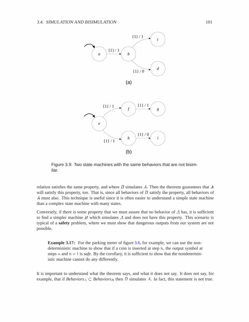
3.4. SIMULATION AND BISIMULATION 101
a b
c
d
{1} / 1
{1} / 1
{1} / 0
(a)
g
e
f
h
{1} / 1
{1} / 1
(b)
{1} / 1
i{1} / 0
Figure 3.9: Two state machines with the same behaviors that are not bisim-ilar.
relation satisfies the same property, and where � simulates �. Then the theorem guarantees that �will satisfy this property, too. That is, since all behaviors of � satisfy the property, all behaviors of� must also. This technique is useful since it is often easier to understand a simple state machinethan a complex state machine with many states.
Conversely, if there is some property that we must assure that no behavior of � has, it is sufficientto find a simpler machine � which simulates � and does not have this property. This scenario istypical of a safety problem, where we must show that dangerous outputs from our system are notpossible.
Example 3.17: For the parking meter of figure 3.6, for example, we can use the non-deterministic machine to show that if a coin is inserted at step �, the output symbol atsteps � and �� is safe. By the corollary, it is sufficient to show that the nondetermin-istic machine cannot do any differently.
It is important to understand what the theorem says, and what it does not say. It does not say, forexample, that if Behaviors� � Behaviors� then � simulates �. In fact, this statement is not true.
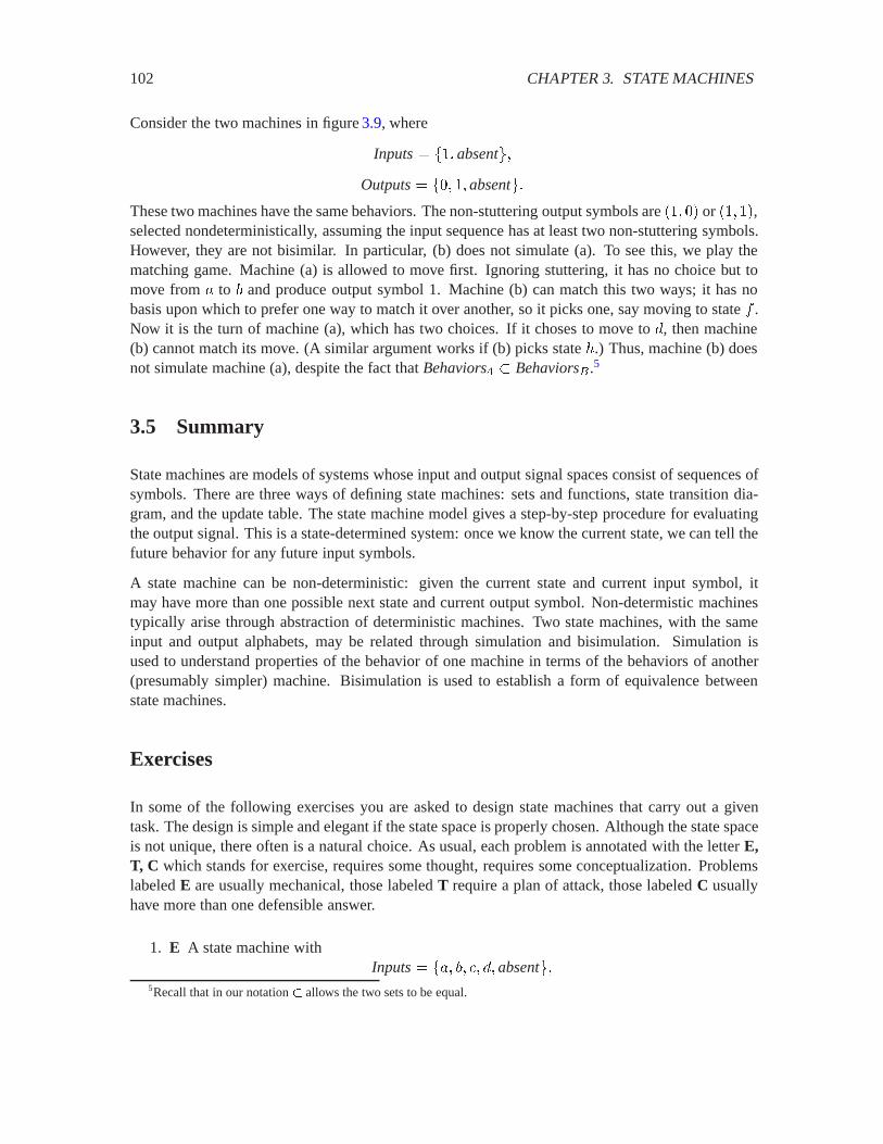
102 CHAPTER 3. STATE MACHINES
Consider the two machines in figure 3.9, where
Inputs� ��absent�Outputs� �� �absent�
These two machines have the same behaviors. The non-stuttering output symbols are �� � or �� �,selected nondeterministically, assuming the input sequence has at least two non-stuttering symbols.However, they are not bisimilar. In particular, (b) does not simulate (a). To see this, we play thematching game. Machine (a) is allowed to move first. Ignoring stuttering, it has no choice but tomove from � to � and produce output symbol 1. Machine (b) can match this two ways; it has nobasis upon which to prefer one way to match it over another, so it picks one, say moving to state � .Now it is the turn of machine (a), which has two choices. If it choses to move to �, then machine(b) cannot match its move. (A similar argument works if (b) picks state �.) Thus, machine (b) doesnot simulate machine (a), despite the fact that Behaviors� � Behaviors� .5
3.5 Summary
State machines are models of systems whose input and output signal spaces consist of sequences ofsymbols. There are three ways of defining state machines: sets and functions, state transition dia-gram, and the update table. The state machine model gives a step-by-step procedure for evaluatingthe output signal. This is a state-determined system: once we know the current state, we can tell thefuture behavior for any future input symbols.
A state machine can be non-deterministic: given the current state and current input symbol, itmay have more than one possible next state and current output symbol. Non-determistic machinestypically arise through abstraction of deterministic machines. Two state machines, with the sameinput and output alphabets, may be related through simulation and bisimulation. Simulation isused to understand properties of the behavior of one machine in terms of the behaviors of another(presumably simpler) machine. Bisimulation is used to establish a form of equivalence betweenstate machines.
Exercises
In some of the following exercises you are asked to design state machines that carry out a giventask. The design is simple and elegant if the state space is properly chosen. Although the state spaceis not unique, there often is a natural choice. As usual, each problem is annotated with the letter E,T, C which stands for exercise, requires some thought, requires some conceptualization. Problemslabeled E are usually mechanical, those labeled T require a plan of attack, those labeled C usuallyhave more than one defensible answer.
1. E A state machine withInputs� ��� �� !� ��absent�
5Recall that in our notation � allows the two sets to be equal.
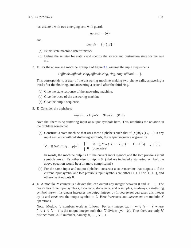
3.5. SUMMARY 103
has a state � with two emerging arcs with guards
guard1� ��and
guard2� ��� �� ��(a) Is this state machine deterministic?
(b) Define the set elsefor state � and specify the source and destination state for the elsearc.
2. E For the answering machine example of figure 3.1, assume the input sequence is
�offhook�offhook� ring�offhook� ring� ring� ring�offhook� ��This corresponds to a user of the answering machine making two phone calls, answering athird after the first ring, and answering a second after the third ring.
(a) Give the state response of the answering machine.
(b) Give the trace of the answering machine.
(c) Give the output sequence.
3. E Consider the alphabets
Inputs� Outputs� Binary� �� �Note that there is no stuttering input or output symbols here. This simplifies the notation inthe problem somewhat.
(a) Construct a state machine that uses these alphabets such that if ����� ���� � is anyinput sequence without stuttering symbols, the output sequence is given by
� � Naturals�� ���� �
� if � � � � ����� ��� ���� �� ����� � �� � � otherwise
In words, the machine outputs 1 if the current input symbol and the two previous inputsymbols are all 1’s, otherwise it outputs 0. (Had we included a stuttering symbol, theabove equation would be a bit more complicated.)
(b) For the same input and output alphabet, construct a state machine that outputs 1 if thecurrent input symbol and two previous input symbols are either �� � � or �� � �, andotherwise it outputs 0.
4. E A modulo � counter is a device that can output any integer between 0 and � � . Thedevice has three input symbols, increment, decrement, and reset, plus, as always, a stutteringsymbol absent; incrementincreases the output integer by 1; decrementdecreases this integerby 1; and resetsets the output symbol to 0. Here incrementand decrementare modulo �operations.
Note: Modulo � numbers work as follows. For any integer ', ' '4� � � 6 where � 6 � � � is the unique integer such that � divides �' � 6�. Thus there are only �distinct modulo-� numbers, namely, � � � � .
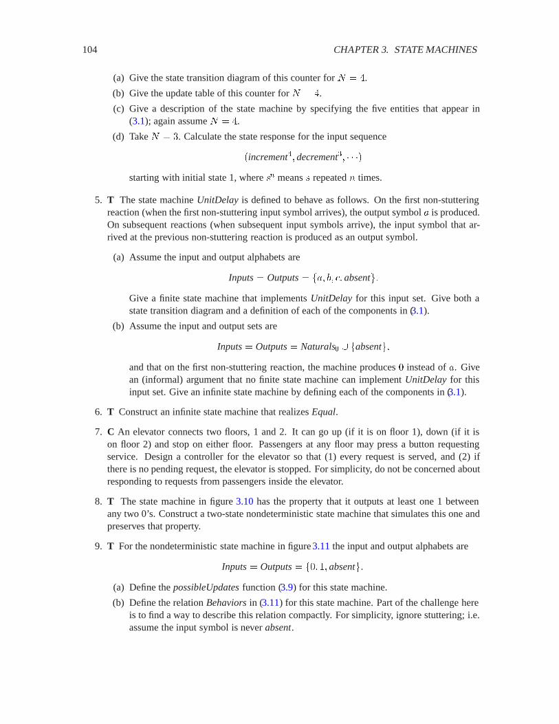
104 CHAPTER 3. STATE MACHINES
(a) Give the state transition diagram of this counter for � � �.
(b) Give the update table of this counter for � � �.
(c) Give a description of the state machine by specifying the five entities that appear in(3.1); again assume � � �.
(d) Take � � �. Calculate the state response for the input sequence
�increment�decrement�� �starting with initial state 1, where �� means � repeated � times.
5. T The state machine UnitDelay is defined to behave as follows. On the first non-stutteringreaction (when the first non-stuttering input symbol arrives), the output symbol � is produced.On subsequent reactions (when subsequent input symbols arrive), the input symbol that ar-rived at the previous non-stuttering reaction is produced as an output symbol.
(a) Assume the input and output alphabets are
Inputs� Outputs� ��� �� !�absent�Give a finite state machine that implements UnitDelay for this input set. Give both astate transition diagram and a definition of each of the components in (3.1).
(b) Assume the input and output sets are
Inputs� Outputs� Naturals� � �absent�and that on the first non-stuttering reaction, the machine produces instead of �. Givean (informal) argument that no finite state machine can implement UnitDelay for thisinput set. Give an infinite state machine by defining each of the components in (3.1).
6. T Construct an infinite state machine that realizes Equal.
7. C An elevator connects two floors, 1 and 2. It can go up (if it is on floor 1), down (if it ison floor 2) and stop on either floor. Passengers at any floor may press a button requestingservice. Design a controller for the elevator so that (1) every request is served, and (2) ifthere is no pending request, the elevator is stopped. For simplicity, do not be concerned aboutresponding to requests from passengers inside the elevator.
8. T The state machine in figure 3.10 has the property that it outputs at least one 1 betweenany two 0’s. Construct a two-state nondeterministic state machine that simulates this one andpreserves that property.
9. T For the nondeterministic state machine in figure 3.11 the input and output alphabets are
Inputs� Outputs� �� �absent�(a) Define the possibleUpdatesfunction (3.9) for this state machine.
(b) Define the relation Behaviorsin (3.11) for this state machine. Part of the challenge hereis to find a way to describe this relation compactly. For simplicity, ignore stuttering; i.e.assume the input symbol is never absent.
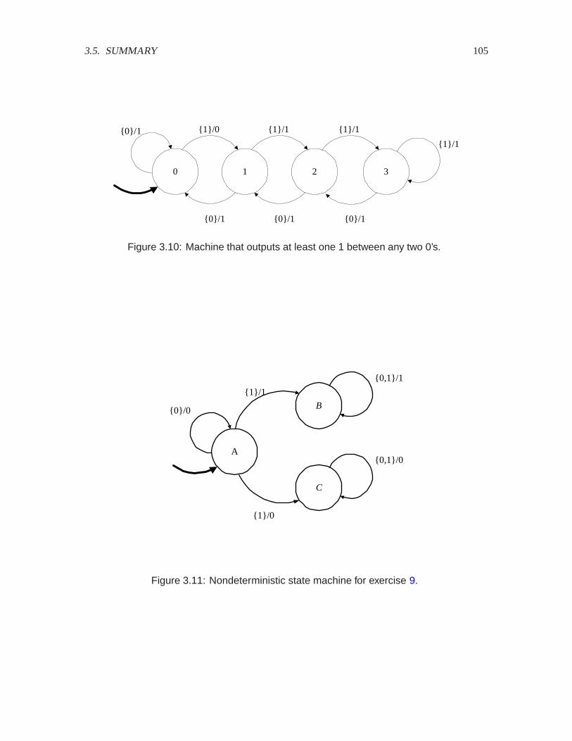
3.5. SUMMARY 105
0 1
{1}/0
{0}/1
2
{1}/1
{0}/1
3
{1}/1
{0}/1
{1}/1{0}/1
Figure 3.10: Machine that outputs at least one 1 between any two 0’s.
A
B
{1}/1
{1}/0
{0,1}/1
C
{0,1}/0
{0}/0
Figure 3.11: Nondeterministic state machine for exercise 9.

106 CHAPTER 3. STATE MACHINES
start 1 11
{1} {1}
{0}{0}
110
{0}/recognize
1100
{0}
{1}
{1}
{0}
{1}
Figure 3.12: A machine that implements CodeRecognizer, but has morestates than the one in figure 3.4.

3.5. SUMMARY 107
a b{1} / 0
c{1} / 0
{1} / 1
Figure 3.13: State machine for problem 11.
a
b
d
{1} / 1
c
{1} / 0
{1} / 1{1} / 0
Figure 3.14: A machine that has more states than it needs.
10. E The state machine in figure 3.12 implements CodeRecognizer, but has more states than theone in figure 3.4. Show that it is equivalent by giving a bisimulation relation with the machinein figure 3.4.
11. E The state machine in figure 3.13 has input and output alphabets
Inputs� �� ��
Outputs� �� � ��where � (short for absent) is the stuttering symbol. State whether each of the following is inthe set Behaviorsfor this machine. In each of the following, the ellipsis “ ” means that thelast symbol is repeated forever. Also, in each case, the input and output signals are given assequences.
(a) ��� � � � � �� �� � � � � ��(b) ��� � � � � �� �� � � � �� ��(c) ���� � �� � �� �� ��� � �� � �� ��(d) ��� � � � � �� �� � �� �� �� ��(e) ��� � � � � �� �� �� � �� �� ��
12. E The state machine in figure 3.14 has
Inputs� ��absent�

108 CHAPTER 3. STATE MACHINES
Outputs� �� �absent�Find a bisimilar state machine with only two states, and give the bisimulation relation.
13. E You are told that state machine � has
Inputs� �� ��absent�
Outputs� �� ��absent�States� ��� �� !� ��
but you are told nothing further. Do you have enough information to construct a state machine� that simulates �? If so, give such a state machine, and the simulation relation.
14. E Construct a state machine with Inputs� �� �absent, Outputs� ���absent, that out-puts � whenever the input signal (without stuttering symbols) contains the sequence �� � �,otherwise it outputs absent. More precisely, if � � ����� ���� � is the input sequencethen � � ����� ���� � is the output sequence, where
���� �
��� if ����� ��� ��� � �� ����� � �� � �absent otherwise
15. T Consider a state machine where
Inputs� ��absent�
Outputs� �� �absent�States� ��� �� !� �� �� ��
initialState� ��
and the updatefunction is given by the following table (ignoring stuttering):
�currentState� inputSymbol� �nextState�outputSymbol�
��� � ��� �
��� � �!� �
�!� � ��� �
��� � ��� �
��� � ��� �
��� � ��� �
(a) Draw the state transition diagram for this machine.
(b) Ignoring stuttering, give the Behaviorsrelation for this machine.
(c) Find a state machine with three states that is bisimilar to this one. Draw that statemachine, and give the bisimulation relation.
Chapter 4
Composing State Machines
We design interesting systems by composing simpler components. Since systems are functions,their composition is function composition, as discussed in section2.1.5. State machines, however,are not given directly as functions that map input sequences into output sequences. Instead, they aregiven procedurally, where the updatefunction defines how to progress from one state to the next.This chapter explains how to define a new state machine that describes a composition of multiplestate machines.
In section 2.3.4 we used a block diagram syntax to define compositions of systems. We will usethe same syntax here, and we will similarly build up an understanding of composition by firstconsidering easy cases. The hardest cases are those where there is feedback, because the inputof one state machine may depend on its own output. It is challenging in this case to come up with aprocedure for updating the state of the composite machine. For some compositions, in fact, it isn’teven possible. Such compositions are said to be ill-formed.
4.1 Synchrony
We consider a set of interconnected components, where each component is a state machine. By“interconnected” we mean that the outputs of one component may be inputs of another. We wish toconstruct a state machine model for the composition of components. Composition has two aspects.The first aspect is straightforward: it specifies which outputs of one component are the inputs ofanother component. These input-output connections are specified using block diagrams.
The second aspect of composition concerns the timing relationships between inputs and outputs. Wechoose a particular style of composition called synchrony. This style dictates that each state ma-chine in the composition reacts simultaneouslyand instantaneously. So a reaction of the compositemachine consists of a set of simultaneous reactions of each of the component machines.
A reaction of the composite machine is triggered by inputs from the environment. Thus, whenareaction occurs is externally determined. This is the same as for a single machine. As with a singlestate machine, a composite machine may stutter. This simply means that each component machine
109

110 CHAPTER 4. COMPOSING STATE MACHINES
stutters.
A system that reacts only in response to external stimulus is said to be reactive. Because ourcompositions are synchronous, they are often called synchronous/reactive systems.
The reactions of the component machines and of the composite machine are viewed as being instan-taneous. That is, a reaction does not take time. In particular, the output symbol from a state machineis viewed as being simultaneouswith the input symbol, without delay. This creates some interestingsubtleties, especially for feedback composition when the input of a state machine is connected to itsown output. We will discuss the ramifications of the synchronous/reactive interpretation below.
Synchrony is a very useful model of the behavior of physical systems. Digital circuits, for example,are almost always designed using this model. Circuit elements are viewed as taking no time tocalculate their outputs given their inputs, and time overall is viewed as progressing in a sequenceof discrete time steps according to ticks of a clock. Of course, the time that it takes for a circuitelement to produce an output cannot ultimately be ignored, but the model is useful because for mostcircuit elements in a complex design, this time can be ignored. Only the time delay of the circuitelements along a critical path affects the overall performance of the circuit.
More recently than for circuits, synchrony has come to be used in software as well. Concurrentsoftware modules interact according to the synchronous model. Languages built on this principleare called synchronous languages. They are used primarily in real-time embedded system1 design.
4.2 Side-by-side composition
A simple form of composition of two state machines is shown in figure4.1. We call this side-by-sidecomposition. Side-by-side composition in itself is not useful, but it is useful in combination withother types of composition. The two state machines in figure 4.1 do not interact with one another.Nonetheless we wish to define a single state machine representing the synchronous operation of thetwo component state machines.
The state space of the composite state machine is simply
States� States� � States� �
We could take the cross product in the opposite order, resulting in a differentbut bisimilar compositestate machine. The initial state is
initialState� �initialState�� initialState���
The input and output alphabets are
Inputs� Inputs� � Inputs� � (4.1)1An embedded system is a computing system (a computer and its software) that is embedded in a larger system that
is not first and foremost a computer. A digital cellular telephone, for example, contains computers that realize the radiomodem and the speech codec. Recent cars contain computers for ignition control, anti-lock brakes, and traction control.Aircraft contain computers for navigation and flight control. In fact, most modern electronic controllers of physicalsystems are realized as embedded systems.
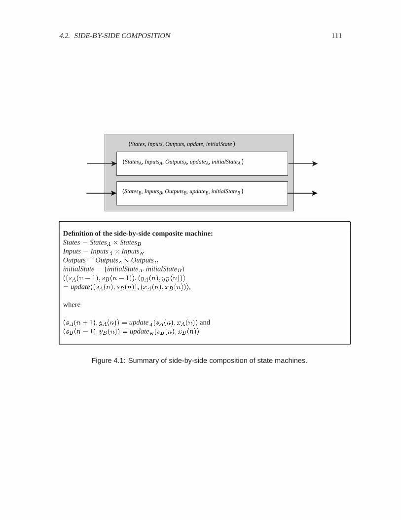
4.2. SIDE-BY-SIDE COMPOSITION 111
(StatesB, InputsB, OutputsB, updateB, initialStateB )
(StatesA, InputsA, OutputsA, updateA, initialStateA )
(States, Inputs, Outputs, update, initialState )
Definition of the side-by-side composite machine:States� States� � States�Inputs� Inputs� � Inputs�Outputs� Outputs� �Outputs�initialState� �initialState�� initialState��������� �� ����� ��� ������� �������� update�������� ������� ������� �������,
where
������ �� ������ � update�������� ������ and������ �� ������ � update�������� ������
Figure 4.1: Summary of side-by-side composition of state machines.

112 CHAPTER 4. COMPOSING STATE MACHINES
Outputs� Outputs� �Outputs�� (4.2)
The update function of the composite machine, update, consists of the update functions of thecomponent machines, side-by-side:
������� �� ����� ��� ������� ������� � update�������� ������� ������� ��������
where������ �� ������ � update�������� �������
and������ �� ������ � update�������� �������
Recall that Inputs� and Inputs� include a stuttering element. This is convenient because it allowsa reaction of the composite when we really want only one of the machines to react. Suppose thestuttering elements are absent� and absent� . Then if the second component of the input symbolis absent� , the reaction of the composite consists only of the reaction of the first machine. Thestuttering element of the composite is the pair of stuttering elements of the component machines,�absent��absent��.
Example 4.1: The side-by-side composition in the top of figure4.2 has the compositemachine with state space
States� States� � States� � ��� �� ��� ��
and alphabets
Inputs� ��� �� �� �� �absent�� �� ��absent��� ��absent��� �absent��absent���
Outputs� ���� !�� ��� !�� �absent�� !�� ���absent��� ���absent��� �absent��absent���The initial state is
initialState� �� ��
The updatefunction can be given as a table, only a part of which is displayed below.The state transition diagram in the lower part of figure 4.2 gives the same part of theupdate function.
current (next state, output) for inputstate (0,0) (1,0) (absent�,0) (1,1) ��� �� ��� !�� ���� �� ��� !�� ((1,1)��absent�� !�) (2,1) ���� �� ��� !�� ��� �� ��� !�� ((2,1), (�absent�� !�)
Notice that if the second component of the input sequence is always absent� , thenthe side-by-side composition behaves essentially as machine �, and if the first compo-nent is always absent�, then it behaves as machine �. The stuttering element of thecomposite is of course the pair �absent��absent��.
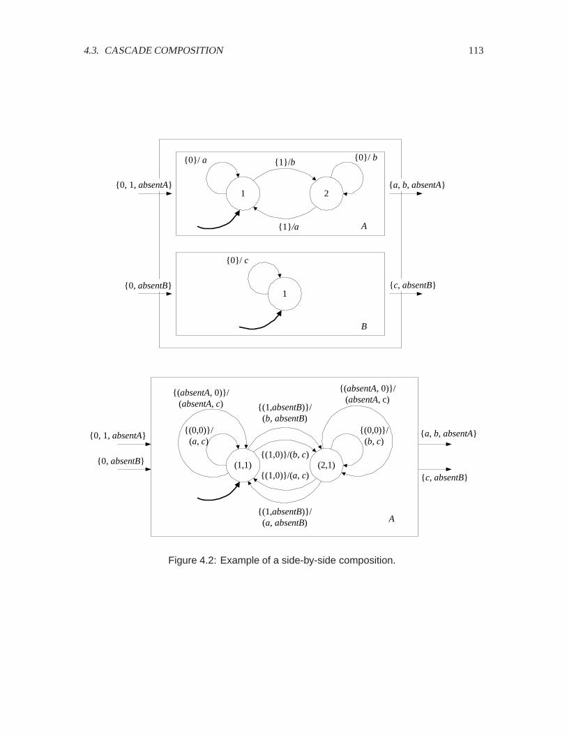
4.3. CASCADE COMPOSITION 113
A
1 2
{1}/b {0}/ b{0}/ a
{1}/a
B
1
{0}/ c
{0, 1, absentA}
{0, absentB} {c, absentB}
A
(1,1) (2,1){(1,0)}/(b, c)
{(0,0)}/(b, c)
{(0,0)}/(a, c)
{(1,0)}/(a, c)
{(absentA, 0)}/(absentA, c)
{(absentA, 0)}/(absentA, c)
{(1,absentB)}/(b, absentB)
{(1,absentB)}/(a, absentB)
{0, 1, absentA}
{0, absentB}
{a, b, absentA}
{c, absentB}
{a, b, absentA}
Figure 4.2: Example of a side-by-side composition.
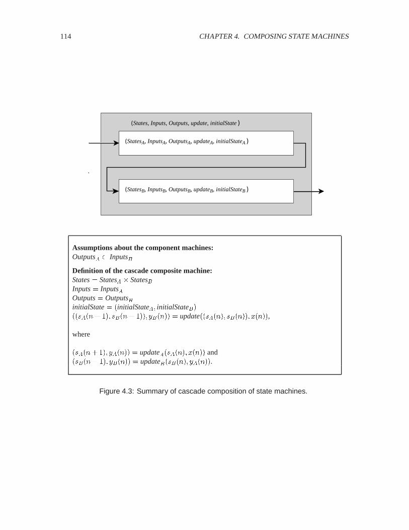
114 CHAPTER 4. COMPOSING STATE MACHINES
(StatesB, InputsB, OutputsB, updateB, initialStateB )
(StatesA, InputsA, OutputsA, updateA, initialStateA )
(States, Inputs, Outputs, update, initialState )
Assumptions about the component machines:Outputs� � Inputs�
Definition of the cascade composite machine:States� States� � States�Inputs� Inputs�Outputs� Outputs�initialState� �initialState�� initialState��������� �� ����� ��� ������ � update�������� ������� �����,
where
������ �� ������ � update�������� ����� and������ �� ������ � update�������� ������.
Figure 4.3: Summary of cascade composition of state machines.
4.3. CASCADE COMPOSITION 115
4.3 Cascade composition
We now interconnect two state machines as shown in figure 4.3, where the output of one is theinput of the other. This is called a cascade composition or a series connection. We define thecomposition so that the component machines react together, synchronously, as one state machine.
Suppose the two state machines are given by
StateMachine� � �States�� Inputs��Outputs��update�� initialState��
andStateMachine� � �States� � Inputs� �Outputs� �update�� initialState���
Let the composition be given by
StateMachine� �States� Inputs�Outputs�update� initialState��
Clearly, for a composition like that in figure 4.3 to be possible we must have
Outputs� � Inputs��
Then any output sequence produced by machine � can be an input sequence for machine �. As aresult,
OutputSignals� � InputSignals� �
This is analogous to a type constraint in programming languages, where in order for two piecesof code to interact, they must use compatible data types. We encountered a similar constraint indiscussing function composition, section 2.1.5.
We are ready to construct a state machine model for this series connection. As noted in the figure,the input alphabet of the composite is
Inputs� Inputs��
The stuttering element of Inputs, of course, is just the stuttering element of Inputs�. The outputalphabet of the composite is
Outputs� Outputs��
The state space of the composite state machine is the product set
States� States� � States� � (4.3)
This asserts that the composite state machine is in state ������� ������ when StateMachine� is instate ����� and StateMachine� is in state �����. The initial state is
initialState� �initialState�� initialState���
We could equally well have defined the states of the composite state machine in the opposite order,
States� States� � States��
116 CHAPTER 4. COMPOSING STATE MACHINES
This would result in a different but bisimilar state machine description (either one simulates theother). Intuitively, it does not matter which of these two choices we make, and we choose (4.3).
To complete the description of the composite machine, we need to define its updatefunction interms of the component machines. Here, a slight subtlety arises. Since we are using synchronouscomposition, the output symbol of machine � is simultaneouswith its input symbol. Thus, in areaction, the output symbol of machine � in that reaction must be available to machine � in thesame reaction. This seems intuitive, but it has some counterintuitive consequences. Although thereactions of machine � and � are simultaneous, we must determine the reaction of � before we candetermine the reaction of �. This apparent paradox is an intrinsic feature of synchronous compo-sition. We will have to deal with it carefully in feedback composition, where it is not immediatelyevident which reactions need to be determined first.
In the cascade composition, it is intuitively clear what we need to do to define the update function.We first determine the reaction of machine �. Suppose that at the �-th reaction the input symbol is���� and the state is ���� � ������� ������, where ����� is the state of machine � and ����� isthe state of machine �. Machine � reacts by updating its state to ����� � and producing outputsymbol �����,
������ �� ������ � update�������� ������ (4.4)
Its output symbol ����� becomes the input symbol to machine �. Machine � reacts by updatingits state to ����� � and producing output symbol �����,
������ �� ������ � update�������� ������� (4.5)
The output of the composite machine, of course, is just the output of machine �, and the next stateof the composite machine is just ������ �� ����� ��, so the composite machine’s updateis
������� �� ����� ��� ������ � update�������� ������� ������
where ������, ������, and ����� are given by (4.4) and (4.5). The definition of the compositemachine is summarized in figure 4.3.
Example 4.2: The cascade composition in figure 4.4 has the composite machine withstate space
States� States� � States� � ��� �� �� �� �� �� �� ��and alphabets
Inputs� Outputs� �� �absent�The initial state is
initialState� �� ��
The updatefunction is given by the table:
current (next state, output) for inputstate 0 1 absent
(0,0) ((0,0),0) ((1,1),1) ((0,0), absent)(0,1) ((0,0),1) ((1,1),0) ((0,1), absent)(1,0) ((1,1),1) ((0,0),0) ((1,0), absent)(1,1) ((1,1),0) ((0,0),1) ((1,1), absent)
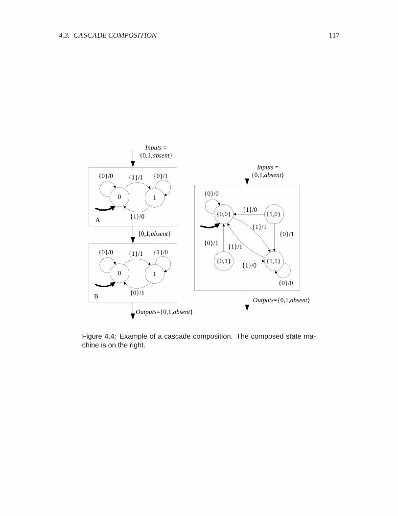
4.3. CASCADE COMPOSITION 117
A
0 1
{1}/1
{1}/0
{0}/0
{0,1,absent}
Inputs ={0,1,absent}
Outputs={0,1,absent}
{0}/1
B
0 1
{1}/1
{0}/1
{0}/0 {1}/0
{0,0}
{1,1}
{1}/1
{1}/1
{0}/0
Inputs ={0,1,absent}
{0}/0
Outputs={0,1,absent}
{1,0}{1}/0
{0}/1{0}/1
{1}/0{0,1}
Figure 4.4: Example of a cascade composition. The composed state ma-chine is on the right.

118 CHAPTER 4. COMPOSING STATE MACHINES
InputsB
InputsA(States, Inputs, Outputs, update, initialState )
OutputsA
OutputsBInputs = InputsA × InputsB
Outputs = OutputsA × OutputsB
Figure 4.5: State machine with product-form inputs and outputs.
The update function is also presented in the state transition diagram of figure4.4. Theself-loops corresponding to the stuttering input symbol absentare not shown in thediagram.
Observe from the table or the diagram that states �� � and �� � are not reachable fromthe initial state. A state � is said to be reachable if some sequence of input symbols cantake the state machine from the initial state to �. This suggests that a simpler machinewith fewer states would exhibit the same input/output behaviors. In fact, notice fromthe table that the input is always equal to the output! A trivial one-state machine canexhibit the same input/output behaviors. (Exercise 8 gives a procedure for calculatingthe reachable states of an arbitrary state machine.)
The simple behavior of the composite machine is not immediately apparent from figure4.4. We have to systematically construct the composite machine to derive this simplebehavior. In fact, this composite machine can be viewed as an encoder and decoder,because the input bit sequence is encoded by a distinctly different bit sequence (theintermediate signal in figure 4.4), and then the second machine, given the intermediatesignal, reconstructs the original.
This particular encoder is known as a differential precoder. It is “differential” inthat when the input symbol is 0, the intermediate signal sample is unchanged from theprevious sample (whether it was 0 or 1), and when the input symbol is 1, the sample ischanged. Thus, the input symbol indicates changein the input with a 1, and no changewith a 0. Differential precoders are used when it is important that the average numberof 1’s and 0’s is the same, regardless of the input sequence that is encoded.
4.4 Product-form inputs and outputs
In the state machine model of (3.1), at each step the environment selects one input symbol to whichthe machine reacts and produces one output symbol. Sometimes we wish to model the fact that someinput values are selected by one part of the environment, while other input values are simultaneouslyselected by another part. Also, some output values are sent to one part of the environment, whileother output values are simultaneously sent to another part. The product-form composition permitsthese models.
The machine in figure 4.5 is shown as a block with two distinct input and output arrows. The figuresuggests that the machine receives inputs from two sources and sends outputs to two destinations.

4.4. PRODUCT-FORM INPUTS AND OUTPUTS 119
In the answering machine example of chapter 3, for instance, the end greetinginput value mightoriginate in a physically different piece of hardware in the machine than the offhookvalue.
The distinct arrows into and out of a block are called ports. Each port has a set of values calledthe port alphabet associated with it, as shown in figure 4.5. Each port alphabet must include astuttering element. The set Inputsof input values to the state machine is the product of the inputsets associated with the ports. Of course, the product can be constructed in any order; each orderingresults in a distinct (but bisimilar) state machine model.
In figure 4.5 there are two input ports and two output ports. The upper input port can present to thestate machine any value in the alphabet Inputs�, which includes absent, its stuttering element. Thelower port can present any value in the set Inputs� , which also includes absent. The input valueactually presented to the state machine in a reaction is taken from the set
Inputs� Inputs� � Inputs��
The stuttering element for this alphabet is the pair �absent�absent�. The output value produced bya reaction is taken from the set
Outputs� Outputs� �Outputs��
If the output of the �-th reaction is ������� ������, then the upper port shows ����� and the lowerport shows �����. These can now be separately presented as inputs to downstream state machines.Again, the stuttering element is �absent�absent�.
Example 4.3: The answering machine of figure 3.1 has input alphabet
Inputs� �ring�offhook�end greeting�end message�
In a typical realization of an answering machine, ring and offhookcome from a subsys-tem (often an ASIC, or application-specific integrated circuit) that interfaces to thetelephone line. The value end greetingcomes from another subsystem, such as a mag-netic tape machine or digital audio storage device, that plays the answer message. Thevalue end messagecomes from a similar, but distinct, subsystem that records incomingmessages. So a more convenient model will show three separate factors for the inputs,as in figure 4.6. That figure also shows the outputs in product form, anticipating thatthe distinct output values will need to be sent to distinct subsystems.
Several features distinguish the diagram in figure4.6 from that of figure 3.1. Each stateexcept the idle state has acquired a self-loop labeled stutter, which is a name for theguard
stutter� ��absent�absent�absent��This self loop prevents the state machine from returning to the idle state (via the elsetransition) when nothing interesting is happening on the inputs. Usually, there will notbe a reaction if nothing interesting is happening on the inputs, but because of synchrony,this machine may be composed with others, and all machines have to react at the sametime. So if anything interesting is happening elsewhere in the system, then this machine
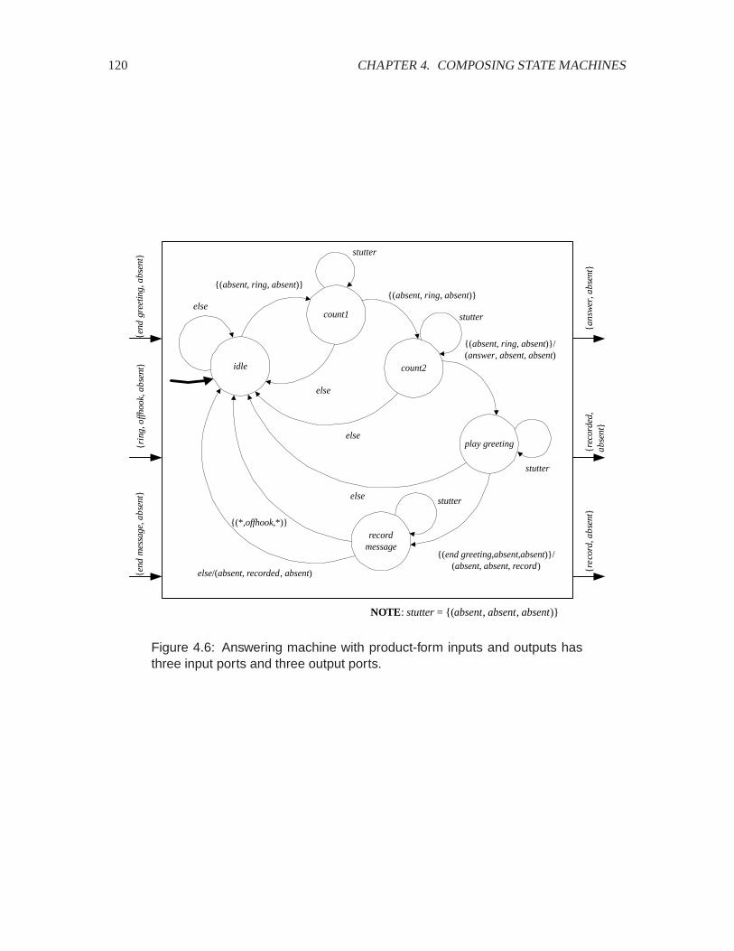
120 CHAPTER 4. COMPOSING STATE MACHINES
idle
count1
count2
{(absent, ring, absent)}{(absent, ring, absent)}
{(absent, ring, absent)}/(answer, absent, absent)
else
elseplay greeting
{(end greeting,absent,absent)}/(absent, absent, record)
recordmessage
else/(absent, recorded , absent)
else
{(*,offhook,*)}
{rin
g, o
ffhoo
k, a
bse
nt}{e
nd m
essa
ge, a
bse
nt}
{rec
orde
d,
ab
sent}
else
{end
gre
etin
g, ab
sent}
{an
swer,
ab
sent}
{re
cord
, ab
sent}
stutter
stutter
stutter
stutter
NOTE: stutter = {(absent, absent, absent)}
Figure 4.6: Answering machine with product-form inputs and outputs hasthree input ports and three output ports.

4.5. GENERAL FEEDFORWARD COMPOSITION 121
(StatesB, InputsB, OutputsB, updateB, initialStateB )
(StatesA, InputsA, OutputsA, updateA, initialStateA )
(States, Inputs, Outputs, update, initialState )
InputsAOutputsA1
OutputsA2 ⊂ InputsB1
InputsB2
OutputsB
OutputsA2
Figure 4.7: More complex composition.
has to react even though nothing interesting is happening here. Recall that such areaction is called a stutter. The state does not change, and the output symbol producedis the stuttering element of the output alphabet.
Each guard now consists of a set of triples, since the product-form input has threecomponents. The shorthand “(*, offhook, *)” on the arc from the record messagestateto the idle state represents a set,
���offhook� �� � ��absent�offhook�absent�� �end greeting�offhook�absent��
�absent�offhook�end message�� �end greeting�offhook�end message��
The “*” is a don’t care or wildcard notation. Anything in its position will trigger theguard.
Because there are three output ports, the output symbols are also triples, but most ofthem are implicitly �absent�absent�absent�.
4.5 General feedforward composition
Given that state machines can have product-form inputs and outputs, it is easy to construct a com-position of state machines that combines features of both the cascade composition of figure4.3 andthe side-by-side composition of figure 4.1. An example is shown in figure 4.7. In that figure,
Outputs� � Outputs�� �Outputs��Inputs� � Inputs�� � Inputs���
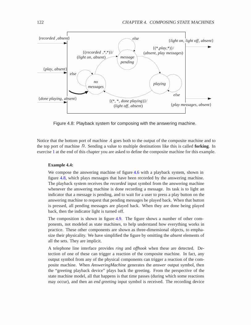
122 CHAPTER 4. COMPOSING STATE MACHINES
nomessages
messagepending
playing
{(recorded,*,*)}/(light on, absent)
{(*,play,*)}/(absent, play messages)
{(*, *, done playing)}/(light off, absent)
else
else
else
{recorded ,absent}
{play, absent}
{done playing, absent}
{light on, light off, absent}
{play messages, absent}
Figure 4.8: Playback system for composing with the answering machine.
Notice that the bottom port of machine � goes both to the output of the composite machine and tothe top port of machine �. Sending a value to multiple destinations like this is called forking. Inexercise 1 at the end of this chapter you are asked to define the composite machine for this example.
Example 4.4:
We compose the answering machine of figure 4.6 with a playback system, shown infigure 4.8, which plays messages that have been recorded by the answering machine.The playback system receives the recordedinput symbol from the answering machinewhenever the answering machine is done recording a message. Its task is to light anindicator that a message is pending, and to wait for a user to press a play button on theanswering machine to request that pending messages be played back. When that buttonis pressed, all pending messages are played back. When they are done being playedback, then the indicator light is turned off.
The composition is shown in figure 4.9. The figure shows a number of other com-ponents, not modeled as state machines, to help understand how everything works inpractice. These other components are shown as three-dimensional objects, to empha-size their physicality. We have simplified the figure by omitting the absentelements ofall the sets. They are implicit.
A telephone line interface provides ring and offhook when these are detected. De-tection of one of these can trigger a reaction of the composite machine. In fact, anyoutput symbol from any of the physical components can trigger a reaction of the com-posite machine. When AnsweringMachinegenerates the answeroutput symbol, thenthe “greeting playback device” plays back the greeting. From the perspective of thestate machine model, all that happens is that time passes (during which some reactionsmay occur), and then an end greetinginput symbol is received. The recording device
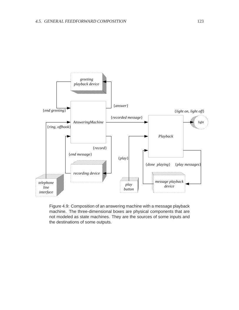
4.5. GENERAL FEEDFORWARD COMPOSITION 123
telephoneline
interface
greetingplayback device
light
playbutton
message playbackdevice
{end greeting}
{ring, offhook}
{end message}
AnsweringMachine
{answer}
{recorded message}
Playback
{play}
{light on, light off}
{done playing} {play messages}
recording device
{record}
Figure 4.9: Composition of an answering machine with a message playbackmachine. The three-dimensional boxes are physical components that arenot modeled as state machines. They are the sources of some inputs andthe destinations of some outputs.
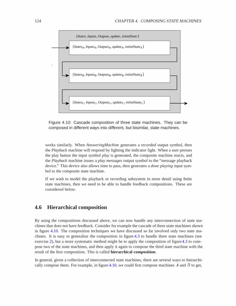
124 CHAPTER 4. COMPOSING STATE MACHINES
(StatesB, InputsB, OutputsB, updateB, initialStateB )
(StatesA, InputsA, OutputsA, updateA, initialStateA )
(States, Inputs, Outputs, update, initialState )
(StatesC, InputsC, OutputsC, updateC, initialStateC )
Figure 4.10: Cascade composition of three state machines. They can becomposed in different ways into different, but bisimilar, state machines.
works similarly. When AnsweringMachinegenerates a recordedoutput symbol, thenthe Playbackmachine will respond by lighting the indicator light. When a user pressesthe play button the input symbol play is generated, the composite machine reacts, andthe Playbackmachine issues a play messagesoutput symbol to the “message playbackdevice.” This device also allows time to pass, then generates a done playinginput sym-bol to the composite state machine.
If we wish to model the playback or recording subsystem in more detail using finitestate machines, then we need to be able to handle feedback compositions. These areconsidered below.
4.6 Hierarchical composition
By using the compositions discussed above, we can now handle any interconnection of state ma-chines that does not have feedback. Consider for example the cascade of three state machines shownin figure 4.10. The composition techniques we have discussed so far involved only two state ma-chines. It is easy to generalize the composition in figure 4.3 to handle three state machines (seeexercise 2), but a more systematic method might be to apply the composition of figure4.3 to com-pose two of the state machines, and then apply it again to compose the third state machine with theresult of the first composition. This is called hierarchical composition.
In general, given a collection of interconnected state machines, there are several ways to hierarchi-cally compose them. For example, in figure 4.10, we could first compose machines � and � to get,

4.7. FEEDBACK 125
f gyx
Figure 4.11: Illustration of a fixed point problem.
say, machine �, and then compose � with � . Alternatively, we could first compose � and � to get,say, machine =, and then compose = and �. These two procedures result in different but bisimilarstate machine models (each simulates the other).
4.7 Feedback
In simple feedback systems, an output from a state machine is fed back as an input to the same statemachine. In more complicated feedback systems, several state machines might be connected in aloop; the output of one eventually affects its own input through some intervening state machines.
Feedback is a subtle form of composition in the synchronous model. In synchronous composition,in a reaction, the output symbol of a state machine is simultaneous with the input symbol. So theoutput symbol of a machine in feedback composition depends on an input symbol that depends onits own output symbol!
We frequently encounter such situations in mathematics. A common problem is to find � such that
� � ���� (4.6)
for a given function � . A solution to this equation, if it exists, is called a fixed point in mathematics.It is analogous to feedback because the ‘output’ ���� of � is equal to its ‘input’ �, and vice versa.The top diagram in figure 4.12 illustrates a similar relationship: the state machine’s output symbolis the same as its (simultaneous) input symbol.
A more complicated problem, involving two equations, is to find � and � so that
� � ����� and � � �����
The analogous feedback composition has two state machines in feedback, with the structure offigure 4.11.2
A fixed-point equation like (4.6) may have no fixed point, a unique fixed point, or multiple fixedpoints. Take for example the function � �Reals� Realswhere �� Reals� ���� � � ��. Inthis case, (4.6) becomes � � � ��, which has no fixed point in the reals. If ���� � � �, (4.6)
2Figure 4.9 would be a feedback composition if any of the three recording or playback devices were modeled as statemachines. In the figure, however, these devices are part of the environment.

126 CHAPTER 4. COMPOSING STATE MACHINES
(StatesA, InputsA, OutputsA, updateA, initialStateA )
(States, Inputs, Outputs, update, initialState )
OutputsA ⊂ InputsA
(StatesA, InputsA, OutputsA, updateA, initialStateA )
(States, Inputs, Outputs, update, initialState )
OutputsA ⊂ InputsA
{react, absent}
Figure 4.12: Feedback composition with no inputs.
becomes � � � �, which has a unique fixed point, � � ��. Lastly, if ���� � ��, (4.6) becomes� � ��, which has two fixed points, � � and � � .
In the context of state machines, a feedback composition with no fixed point in some reachable stateis a defective design; we call such a composition ill-formed. We can not evaluate an ill-formedcomposition. Usually, we also wish to exclude feedback compositions that have more than one non-stuttering fixed point in some reachable state. So these too are ill-formed. A feedback compositionwith a unique non-stuttering fixed point in all reachable states is well-formed. Fortunately, it is easyto construct well-formed feedback compositions, and they prove surprisingly useful. We explore thisfurther, beginning with a somewhat artificial case of feedback composition with no inputs.
4.7.1 Feedback composition with no inputs
The upper state machine in figure 4.12 has an output port that feeds back to its input port. We wishto construct a state machine model that hides the feedback, as suggested by the figure. The resultwill be a state machine with no input. This does not fit our model, which requires the environmentto provide inputs to which the machine reacts. So we artificially provide an input alphabet
Inputs� �react�absent�as suggested in the lower machine in figure4.12. We interpret the input symbol reactas a commandfor the internal machine to react, and the input symbol absentas a command for the internal machineto stutter. The output alphabet is
Outputs� Outputs��
This is an odd example of a synchronous/reactive system because of the need for this artificialinput alphabet. Typically, however, such a system will be composed with others, as suggested in

4.7. FEEDBACK 127
(StatesA, InputsA, OutputsA, updateA, initialStateA )
(States, Inputs, Outputs, update, initialState )
OutputsA ⊂ InputsA
(StatesB, InputsB, OutputsB, updateB, initialStateB )
Figure 4.13: Feedback composition composed with another state machine.
figure 4.13. That composition does have an external input. So the overall composition, includingthe component with no external input, reacts whenever an external input symbol is presented, andthere is no need for the artificial inputs. Of course when a stuttering element is provided to thecomposite, all components stutter.
Although it is not typical, we first consider the example in figure 4.12 because the formulation ofthe composition is simplest. We will augment the model to allow inputs after this.
In figure 4.12, for the feedback connection to be possible, of course, we must have
Outputs� � Inputs��
Suppose the current state at the �-th reaction is ���� States�. The problem is to find the outputsymbol ���� Outputs�. Since ���� is also the input symbol, it must satisfy
����� �� ����� � update������� ������
where ��� � � is the next state. The difficulty here is that the “unknown” ���� appears on bothsides. Once we find ����, ����� is immediately determined by the update� function. To simplifythe discussion, we get rid of ���� � by working with the function
output��States� � Inputs� � Outputs�
This function gives the output symbol as a function of the current state and the current input symbol,as we saw in section 3.1.1. So our problem is: given the current state ���� and the known functionoutput�, find ���� such that
���� � output������� ������ (4.7)
Here ���� is a known constant, so the equation is of the form (4.6), and its solution, if it exists, is afixed point.
One solution that is always available is to stutter, i.e.,
���� � absent� (and then ���� � � ����)�

128 CHAPTER 4. COMPOSING STATE MACHINES
since absent� output�������absent�, assuming that absentis the stuttering input symbol for ma-chine �. But this is not an interesting solution, since the state does not change. We want to find anon-stuttering solution for ����.
We say that the composition of figure 4.12 is well-formed if for every reachable ���� States�,there is a unique non-stuttering output symbol ���� that solves (4.7); otherwise, the composition isill-formed. If the composition is well-formed, the composite machine definition is:
States� States�Inputs� �react�absentOutputs� Outputs�initialState� initialState�
update������ ����� �
��������
update������� ������where ���� �� absentuniquely satisfies (4.7) if ���� � react
������ ����� if ���� � absent
Notice that the composite machine is defined only if the composition is well-formed, i.e., there isa unique ���� that satisfies (4.7). If there is no such ����, the composition is ill-formed and thecomposite machine is not defined.
The next example illustrates the difference between well-formed and ill-formed compositions. Itwill suggest a procedure to solve (4.7) in the important special case of systems with state-determinedoutput.
Example 4.5: Consider the three feedback compositions in figure 4.14. In all cases,the input and output alphabets of the component machines are
Inputs� � Outputs� � �true� false�absent�
The input alphabet to the compositemachine is �react�absent, as in figure4.12, butwe do not show this (to reduce clutter in the figure). We want to find a non-stutteringsolution ���� of (4.7). Since the output symbol is also the input symbol, we are lookingfor a non-stuttering input symbol.
Consider the top machine first. Suppose the current state is the initial state, ���� �. There are two outgoing arcs, and for a non-stuttering input symbol, both produce���� � false, so we can conclude that the output symbol of the machine is false. Sincethe output symbol is false, then the input symbol is also false, and the non-stutteringfixed point of (4.7) is unique,
output��� false� � false�
The state transition taken by the reaction goes from state 1 to state 2.
Suppose next that the current state is ���� � �. Again, there are two outgoing arcs.Both arcs produce output symbol true for a non-stuttering input symbol, so we can

4.7. FEEDBACK 129
1 2
{false}/false
{true}/true
{true}/false {false}/true
(a)
(b)
(c)
1 2
{false}/false
{true}/false
{true}/false {false}/true
1 2
{false}/false
{true}/true
{true}/true {false}/false
Figure 4.14: Three examples of feedback composition. Examples (b) and(c) are ill-formed. Composition (b) has no non-stuttering fixed point in state2, while composition (c) has two non-stuttering fixed points in either state.
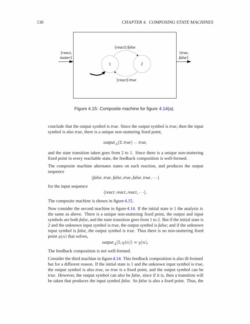
130 CHAPTER 4. COMPOSING STATE MACHINES
1 2
{react}/false
{react}/true
{react,stutter}
{true,false}
Figure 4.15: Composite machine for figure 4.14(a).
conclude that the output symbol is true. Since the output symbol is true, then the inputsymbol is also true, there is a unique non-stuttering fixed point,
output���� true� � true�
and the state transition taken goes from 2 to 1. Since there is a unique non-stutteringfixed point in every reachable state, the feedback composition is well-formed.
The composite machine alternates states on each reaction, and produces the outputsequence
�false� true� false� true� false� true� �for the input sequence
�react� react� react� ��The composite machine is shown in figure 4.15.
Now consider the second machine in figure 4.14. If the initial state is 1 the analysis isthe same as above. There is a unique non-stuttering fixed point, the output and inputsymbols are both false, and the state transition goes from 1 to 2. But if the initial state is2 and the unknown input symbol is true, the output symbol is false; and if the unknowninput symbol is false, the output symbol is true. Thus there is no non-stuttering fixedpoint ���� that solves,
output���� ����� � �����
The feedback composition is not well-formed.
Consider the third machine in figure 4.14. This feedback composition is also ill-formedbut for a different reason. If the initial state is 1 and the unknown input symbol is true,the output symbol is also true, so true is a fixed point, and the output symbol can betrue. However, the output symbol can also be false, since if it is, then a transition willbe taken that produces the input symbol false. So falseis also a fixed point. Thus, the
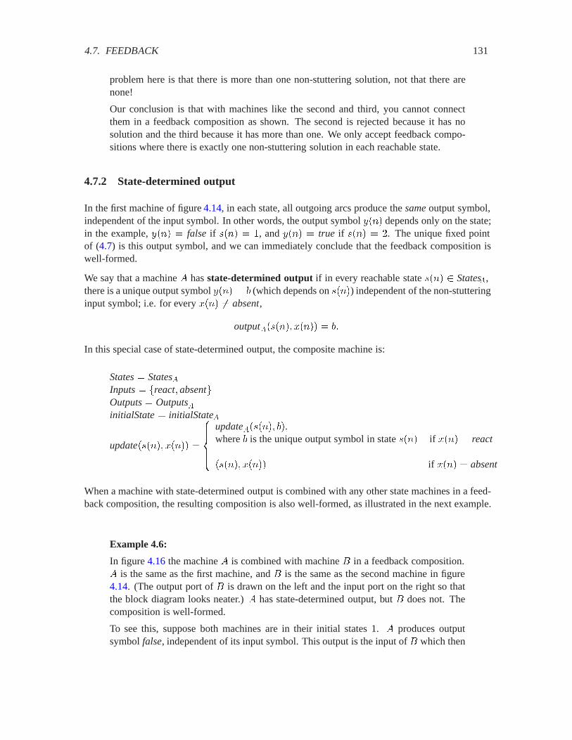
4.7. FEEDBACK 131
problem here is that there is more than one non-stuttering solution, not that there arenone!
Our conclusion is that with machines like the second and third, you cannot connectthem in a feedback composition as shown. The second is rejected because it has nosolution and the third because it has more than one. We only accept feedback compo-sitions where there is exactly one non-stuttering solution in each reachable state.
4.7.2 State-determined output
In the first machine of figure 4.14, in each state, all outgoing arcs produce the sameoutput symbol,independent of the input symbol. In other words, the output symbol ���� depends only on the state;in the example, ���� � false if ���� � , and ���� � true if ���� � �. The unique fixed pointof (4.7) is this output symbol, and we can immediately conclude that the feedback composition iswell-formed.
We say that a machine � has state-determined output if in every reachable state ���� States�,there is a unique output symbol ���� � � (which depends on ����) independent of the non-stutteringinput symbol; i.e. for every ���� �� absent,
output������� ����� � ��
In this special case of state-determined output, the composite machine is:
States� States�Inputs� �react�absentOutputs� Outputs�initialState� initialState�
update������ ����� �
��������
update������� ���where � is the unique output symbol in state ���� if ���� � react
������ ����� if ���� � absent
When a machine with state-determined output is combined with any other state machines in a feed-back composition, the resulting composition is also well-formed, as illustrated in the next example.
Example 4.6:
In figure 4.16 the machine � is combined with machine � in a feedback composition.� is the same as the first machine, and � is the same as the second machine in figure4.14. (The output port of � is drawn on the left and the input port on the right so thatthe block diagram looks neater.) � has state-determined output, but � does not. Thecomposition is well-formed.
To see this, suppose both machines are in their initial states 1. � produces outputsymbol false, independent of its input symbol. This output is the input of � which then
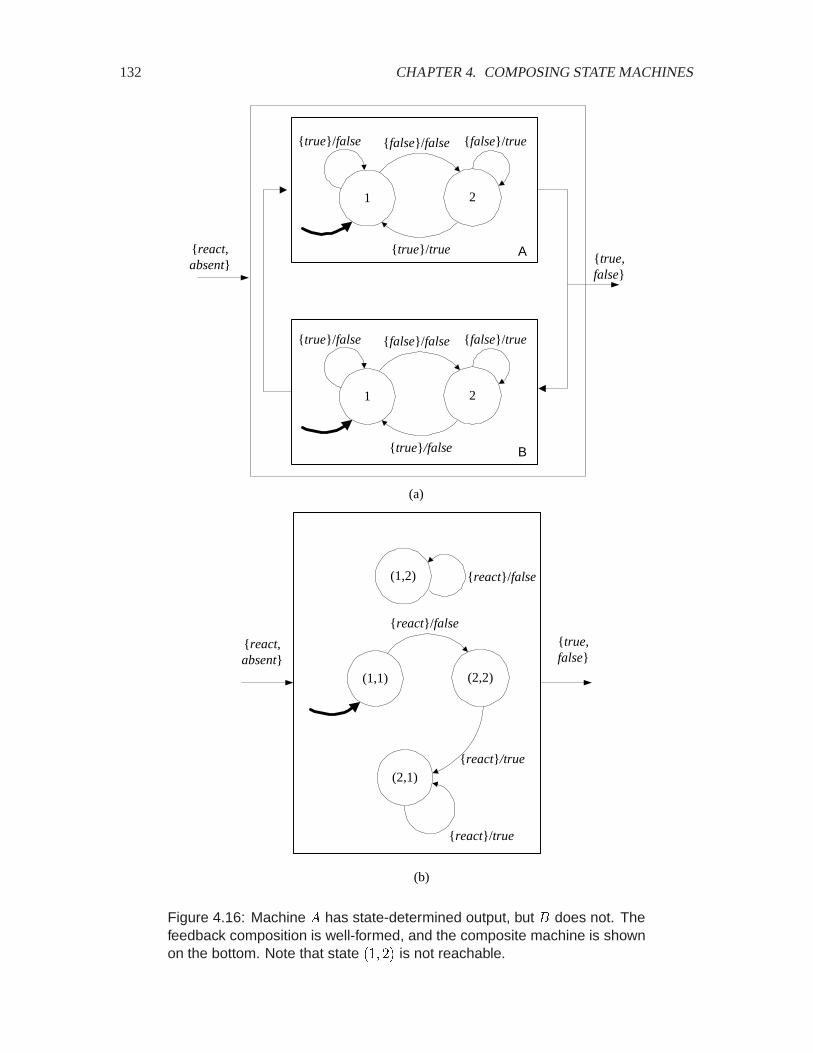
132 CHAPTER 4. COMPOSING STATE MACHINES
1 2
{false}/false
{true}/true
{true}/false {false}/true
1 2
{false}/false
{true}/false
{true}/false {false}/true
B
A{react,absent} {true,
false}
(1,1) (2,2)
{react}/false
{react}/true
{react,absent}
{true,false}
(1,2) {react}/false
{react}/true
(2,1)
(a)
(b)
Figure 4.16: Machine � has state-determined output, but � does not. Thefeedback composition is well-formed, and the composite machine is shownon the bottom. Note that state �� �� is not reachable.

4.7. FEEDBACK 133
produces output symbol falseand makes the transition to state 2. The output symbolfalseof � is the input to � which makes the transition to its state 2. (� and � maketheir state transitions together in our synchronous/reactive model.) We can determinethe output symbol and transition in the same way for all other states. The state diagramof the composite machine is shown in the figure on the right. Note that state �� �� isnot reachable from the initial state �� �, so we could have ignored it in determiningwhether the composition is well-formed.
The input alphabet of the composite machine is �react�absent, taking absentas thestuttering input symbol. The output alphabet is the same as the output alphabet of �,�true� false�absent. The state space is States��States� . The updatefunction is givenby the table:
current (next state, output) for inputstate react absent
(1,1) ((2,2),false) ((1,1),absent)(2,2) ((2,1),true) ((2,2), absent)(1,2) ((1,2),false) ((1,2), absent)(2,1) ((2,1),true) ((2,1), absent)
It is possible for a machine without state-determined outputs to be placed in a well-formed feedbackcomposition as illustrated in the next example.
Example 4.7: Consider the example in figure 4.17. For the component machine, theoutput alphabet is Outputs� � �true� false�maybe�absent, and the input alphabet isInputs� � �true� false�absent. The stuttering element is absent. The machine doesnot have state-determined output because, for instance, the outgoing arcs from state1 can produce both maybeand false. Nevertheless, equation (4.7) has a unique non-stuttering fixed point in each state:
output��� false� � false� and output���� true� � true�
So the feedback composition is well-formed. The composite machine is shown on thebottom.
It can be considerably harder to find the behavior of a feedback composition without state-determinedoutputs, even if the composition is well-formed. Below, in section4.7.4, we give a constructive pro-cedure that often works to quickly find a fixed point, and to determine whether it is unique. However,even that procedure does not always work (and in fact, will fail on example 4.7). If the input al-phabet is finite, the only strategy that always works is to try all possible output values ���� is (4.7)for each reachable state ����. Before discussing this procedure, we generalize to more interestingfeedback compositions.

134 CHAPTER 4. COMPOSING STATE MACHINES
{react,absent}
{true,false}
1 2
{false}/false
{true}/true
{true}/maybe
{false}/maybe
1 2
{react}/false
{react}/true
{react,absent}
{true,false}
A
(a)
(b)
Figure 4.17: Machine � does not have state-determined outputs, but thefeedback composition is well-formed. The machine on the bottom is thecomposite machine.
4.7. FEEDBACK 135
(StatesA, InputsA, OutputsA, updateA, initialStateA )
(States, Inputs, Outputs, update, initialState )InputsA1 OutputsA1
OutputsA2 ⊂ InputsA2
A
InputsA2 OutputsA2
Figure 4.18: Feedback composition of a state machine.
4.7.3 Feedback composition with inputs
Now consider the state machine in figure 4.18. It has two input and output ports. The second outputport feeds back to the second input port. We wish to construct a state machine model that hidesthe feedback, as suggested by the figure, and becomes a simple input/output state machine. This issimilar to the example in figure 4.12, but now there is an additional input and an additional output.The procedure for finding the composite machine is similar, but the notation is more cumbersome.Given the current state and the current external input symbol, we must determine the “unknown”output symbol.
The inputs and outputs of machine � are in product form:
Inputs� � Inputs�� � Inputs���
Outputs� � Outputs�� �Outputs���
For the feedback composition to be possible we must have
Outputs�� � Inputs���
The output function of � is
output� � States� � Inputs� � Outputs��
It is convenient to write it in product form as,
output� � �output���output����
whereoutput�� � States� � Inputs� � Outputs���
gives the output symbol at the first output port and
output�� � States� � Inputs� � Outputs���
136 CHAPTER 4. COMPOSING STATE MACHINES
gives the output symbol at the second output port.
Suppose we are given that at the �-th reaction, the current state of � is ���� and the current externalinput symbol is ����� Inputs��. Then the problem is to find the “unknown” output symbol������� ������ Outputs� such that
output������� ������� ������� � ������� ������� (4.8)
The symbol ����� appears on both sides because the second input ����� to machine � is equal to�����. In terms of the product form, (4.8) is equivalent to two equations:
output�������� ������� ������� � ������ (4.9)
output�������� ������� ������� � ������ (4.10)
In these equations, ���� and ����� are known, while ����� and ����� are unknown. Observe that if(4.10) has a unique solution �����, then the input symbol to � is ������� ������ and the next state����� and output symbol ����� are determined. So the fixed point equation (4.10) plays the samerole as (4.7).
We say that the composition of figure4.18 is well-formed if for every reachable state ���� States�and for every external input symbol ����� Inputs��, there is a unique non-stuttering outputsymbol ����� Outputs�� that solves (4.10). If the composition is well-formed, the compositemachine definition is:
States� States�Inputs� Inputs��Outputs� Outputs��initialState� initialState�update������ ����� � �nextState������ ������output������ ������:nextState������ ����� � nextState������� ������ ������� andoutput������ ����� � output������� ������ �������, where ����� is the unique solu-
tion of (4.10).
(The ���.�� function is defined in section 3.1.1.)
In the following example, we illustrate the procedure for defining the composition machine given asets and functions description (3.1) for the component machine �.
Example 4.8: Figure 4.19 shows a feedback composition, where component machine� has two input ports and one output port,
Inputs� � Reals� Reals� Outputs� � Reals�
and states States� � Reals. Thus � has infinite input and output alphabets andinfinitely many states. At the �-th reaction, the pair of input values is denoted by������� ������, the current state by ����, the next state by ��� � �, and the outputsymbol by ����. In terms of these, the update function is given by
������� ����� � update������� ������� ������� � �������������������� ������
Equivalently,

4.7. FEEDBACK 137
xy
A
∀ n ∈ Reals,s(n+1) = 0.5s(n) + x1(n) + x2(n)y(n) = s(n)
x y∀ n ∈ Reals,s(n+1) = 1.5s(n) + x(n)y(n) = s(n)
x1
x2
Figure 4.19: Machine� has two input ports and one output port. The outputport is connected to the second input port. The composition is well-formed.The composite machine is shown at the bottom.
���� � � nextState������� ������� ������� � ������ � ����� � ��������� � output������� ������� ������� � ����
Thus, the component machine � has state-determined output. The feedback connectsthe output port to the second input port, so ����� � ����. Given the current state ����and the external input symbol ���� at the first input port, (4.10) becomes,
output������� ������� ������� � ������
which gives���� � ������
So the composite machine is defined by
Inputs= Reals, Outputs= Reals, States= Realsupdate������ ����� � ������������������ ����� � ������������� ������
Note that the input to the composite machine is a scalar. The composite machine isshown in the lower part of the figure.
4.7.4 Constructive procedure for feedback composition
Our examples so far involve one or two state machines and a feedback loop. If any machine in theloop has state determined output, then finding the fixed point is easy. Most interesting designs are
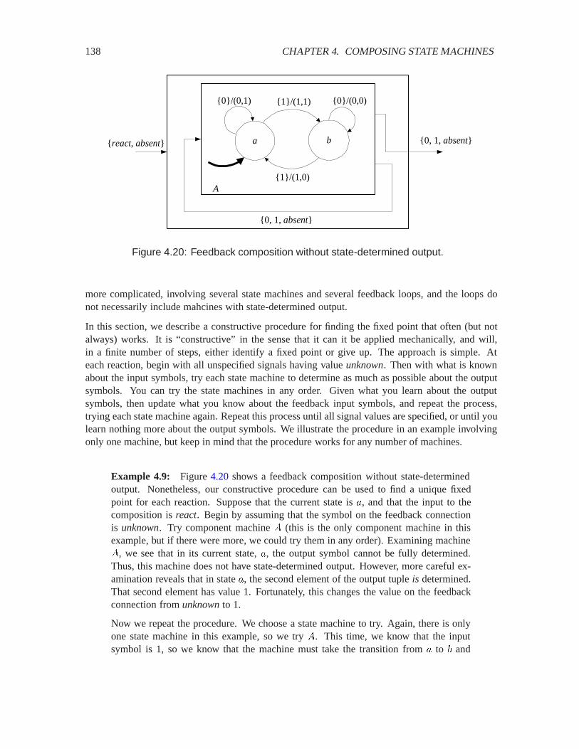
138 CHAPTER 4. COMPOSING STATE MACHINES
a b
{1}/(1,1)
{1}/(1,0)
{0}/(0,1) {0}/(0,0)
{0, 1, absent}
{0, 1, absent}{react, absent}
A
Figure 4.20: Feedback composition without state-determined output.
more complicated, involving several state machines and several feedback loops, and the loops donot necessarily include mahcines with state-determined output.
In this section, we describe a constructive procedure for finding the fixed point that often (but notalways) works. It is “constructive” in the sense that it can it be applied mechanically, and will,in a finite number of steps, either identify a fixed point or give up. The approach is simple. Ateach reaction, begin with all unspecified signals having value unknown. Then with what is knownabout the input symbols, try each state machine to determine as much as possible about the outputsymbols. You can try the state machines in any order. Given what you learn about the outputsymbols, then update what you know about the feedback input symbols, and repeat the process,trying each state machine again. Repeat this process until all signal values are specified, or until youlearn nothing more about the output symbols. We illustrate the procedure in an example involvingonly one machine, but keep in mind that the procedure works for any number of machines.
Example 4.9: Figure 4.20 shows a feedback composition without state-determinedoutput. Nonetheless, our constructive procedure can be used to find a unique fixedpoint for each reaction. Suppose that the current state is �, and that the input to thecomposition is react. Begin by assuming that the symbol on the feedback connectionis unknown. Try component machine � (this is the only component machine in thisexample, but if there were more, we could try them in any order). Examining machine�, we see that in its current state, �, the output symbol cannot be fully determined.Thus, this machine does not have state-determined output. However, more careful ex-amination reveals that in state �, the second element of the output tuple is determined.That second element has value 1. Fortunately, this changes the value on the feedbackconnection from unknownto 1.
Now we repeat the procedure. We choose a state machine to try. Again, there is onlyone state machine in this example, so we try �. This time, we know that the inputsymbol is 1, so we know that the machine must take the transition from � to � and

4.7. FEEDBACK 139
produce the output tuple �� �. This results in all symbols being known for the reaction,so we are done evaluating the reaction.
Now assume the current state is �. Again, the feedback symbol is initially unknown,but once again, trying �, we see that the second element of the output tuple must be 0.Thus, we change the feedback symbol from unknownto 0 and try the machine again.This time, its input is 0, so it must take the self loop back to � and produce the outputtuple �� �.
Recall that the set Behaviorsis the set of all ��� �� such that � is an input sequence and� is an output sequence. For this machine, ignoring stuttering, the only possible inputsequence is �react� react� react� �. We have just determined that the resulting outputsequence is �� � � � �. Thus, ignoring stuttering,
Behaviors� ���react� react� react� �� �� � � � ���Of course, we should take into account stuttering, so this set needs to be augmentedwith all ��� �� pairs that look like the one above but have stuttering symbols inserted.
This procedure can be applied in general to any composition of state machines. If the procedurecan be applied successfully (nothing remains unknown) for all reachable states of the composition,then the composition is well-formed. The following example applies the procedure to a more com-plicated example.
Example 4.10: We add more detail to the message recorder in figure4.9. In particular,as shown in figure 4.21, we wish to model the fact that the message recorder stopsrecording when either it detects a dialtone or when a timeout period is reached. Thisis modeled by a two-state finite state machine, shown in figure 4.22. Note that thismachine does not have state-determined output. For example, in state idle, the outputcould be �absent� start recording� or it could be �absent�absent� when the input is notthe stuttering input.
The MessageRecorderand AnsweringMachinestate machines form a feedback loop.Let us verify that composition is well-formed. First, note that in the idle state of theMessageRecorder, the upper output symbol is known to be absent(see figure 4.22).Thus, only in the recordingstate is there any possibility of a problem that would lead tothe composition being ill-formed. In that state, the output symbol is not known unlessthe input symbols are known. However, notice that the recordingstate is entered onlywhen a record input symbol is received. In figure4.6, you can see that the recordvalueis generated only when entering state record message. But in all arcs emerging fromthat state, the lower output symbol of AnsweringMachinewill always be absent; theinput symbol does not need to be known to know that. Continuing this reasoning byconsidering all possible state transitions from this point, we can convince ourselves thatthe feedback loop is well-formed.
The sort of reasoning in this more complicated example is difficult and error-prone for even mod-erate compositions of state machines. It is best automated. Compilers for synchronous languages

140 CHAPTER 4. COMPOSING STATE MACHINES
telephoneline interface
greeting playbackdevice
light
playbutton
message playbackdevice
{end greeting}
{ring, offhook}
{end message}
AnsweringMachine
{answer}
{recorded message}
{record}
Playback{play}
{light on, light off}
{done playing} {play messages}
recording device
MessageRecorder{dialtone}
{start recording}{timeout}
Figure 4.21: Answering machine composition with feedback. The absentelements are not shown (to reduce clutter).
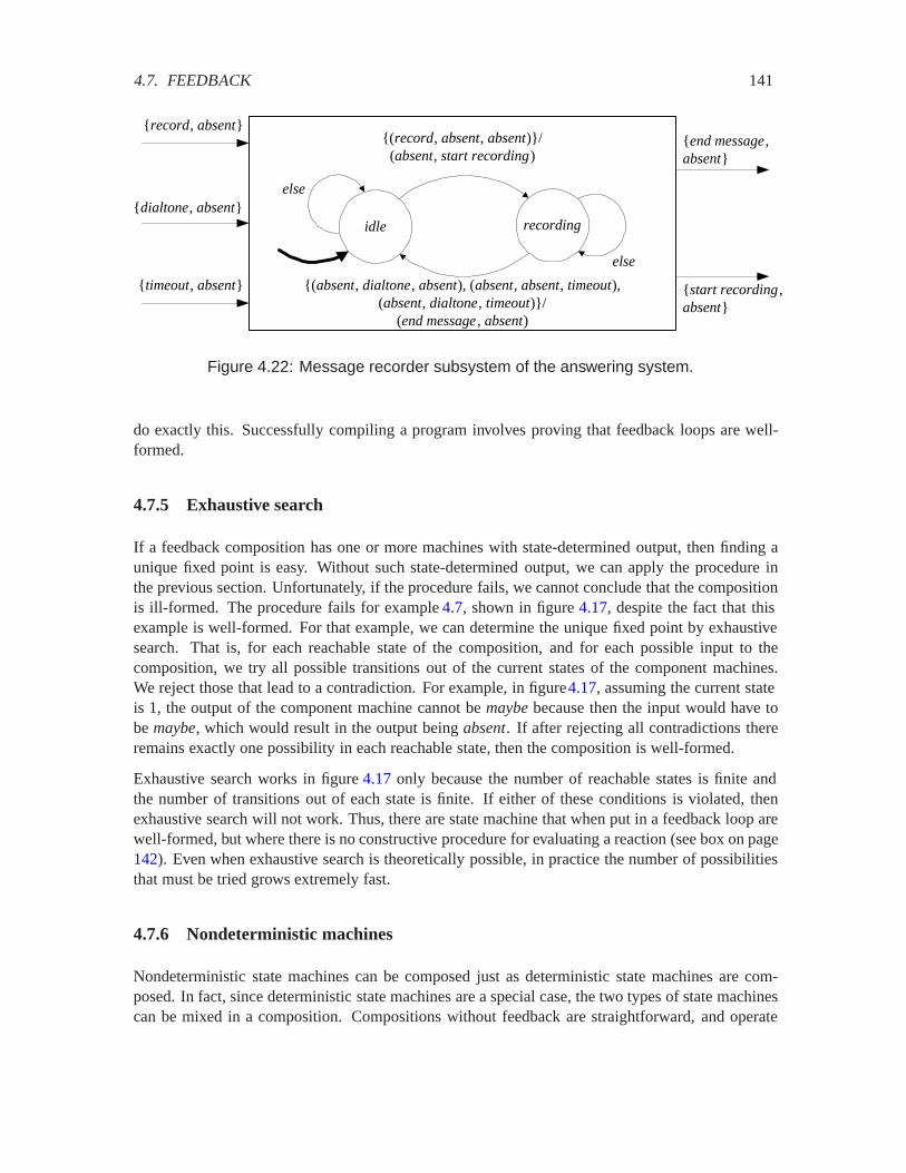
4.7. FEEDBACK 141
idle recording
{(record, absent, absent)}/(absent, start recording)
{(absent, dialtone, absent), (absent, absent, timeout),(absent, dialtone, timeout)}/
(end message, absent)
else
else
{record, absent}
{dialtone, absent}
{timeout, absent}
{end message,absent}
{start recording,absent}
Figure 4.22: Message recorder subsystem of the answering system.
do exactly this. Successfully compiling a program involves proving that feedback loops are well-formed.
4.7.5 Exhaustive search
If a feedback composition has one or more machines with state-determined output, then finding aunique fixed point is easy. Without such state-determined output, we can apply the procedure inthe previous section. Unfortunately, if the procedure fails, we cannot conclude that the compositionis ill-formed. The procedure fails for example 4.7, shown in figure 4.17, despite the fact that thisexample is well-formed. For that example, we can determine the unique fixed point by exhaustivesearch. That is, for each reachable state of the composition, and for each possible input to thecomposition, we try all possible transitions out of the current states of the component machines.We reject those that lead to a contradiction. For example, in figure4.17, assuming the current stateis 1, the output of the component machine cannot be maybebecause then the input would have tobe maybe, which would result in the output being absent. If after rejecting all contradictions thereremains exactly one possibility in each reachable state, then the composition is well-formed.
Exhaustive search works in figure 4.17 only because the number of reachable states is finite andthe number of transitions out of each state is finite. If either of these conditions is violated, thenexhaustive search will not work. Thus, there are state machine that when put in a feedback loop arewell-formed, but where there is no constructive procedure for evaluating a reaction (see box on page142). Even when exhaustive search is theoretically possible, in practice the number of possibilitiesthat must be tried grows extremely fast.
4.7.6 Nondeterministic machines
Nondeterministic state machines can be composed just as deterministic state machines are com-posed. In fact, since deterministic state machines are a special case, the two types of state machinescan be mixed in a composition. Compositions without feedback are straightforward, and operate

142 CHAPTER 4. COMPOSING STATE MACHINES
Probing further: Constructive Semantics
The term “semantics” means meaning. We have defined the meaning of composi-tions of state machines using the notion of synchrony, which makes feedback com-positions particularly interesting. When we define “well-formed,” we are, in effect,limiting the compositions that are valid. Compositions that are not well-formed falloutside our synchronous semantics. They have no meaning.
One way to define the semantics of a composition is to give a procedure for evalu-ating the composition (the resulting procedure is called an operational semantics).We have given three successively more difficult procedures for evaluating a reac-tion of a composition of state machines with feedback. If at least one machine ineach directed loop has state-determined output, then it is easy to evaluate a reaction.If not, we can apply the constructive procedure of section4.7.4. However, that pro-cedure may result in some feedback connections remaining unknowneven thoughthe composition is well-formed. The ultimate procedure is exhaustive search, asdescribed in section 4.7.5. However, exhaustive search is not always possible, andeven when it is theoretically possible, the number of possibilities to explore may beso huge that it is not practical. There are state machines that when put in a feedbackloop are well-formed, but where there is no constructive procedure for evaluating areaction, and no constructive way to demonstrate that they are well-formed. Thus,there is no operational semantics for our feedback compositions.
This situation is not uncommon in computing and in mathematics. Kurt Godel’sfamous incompleteness theorem (1931), for example, states (loosely) that in anyformal logical system, there are statements that are true but not provable. This isanalogous in that we can have feedback compositions that are well-formed, but wehave no procedure that will always work to demonstrate that they are well-formed.Around the same time, Alan Turing and Alonzo Church demonstrated that there arefunctions that cannot be computed by any procedure.
To deal with this issue, Gerard Berry has proposed that synchronous compositionhave a constructive semantics, which means precisely that well-formed composi-tions are defined to be those for which the constructive procedure of section4.7.4works. When that procedure fails, we simply declare the composition to be unac-ceptable. This is pragmatic solution, and in many situations, it is adequate. How-ever, particularly in the field of feedback control, it proves too restrictive. Mostfeedback control systems in practical use would be rejected by this semantics.
See G. Berry, The Constructive Semantics of Pure Esterel, Book Draft,http://www.esterel-technologies.com/corporate/berry.htm.

4.8. SUMMARY 143
almost exactly as described above (see exercises14 and 15). Compositions with feedback require asmall modification to our evaluation process.
Recall that to evaluate the reaction of a feedback composition, we begin by setting to unknownanyinput symbols that are not initially known. We then proceed through a series of rounds where ineach round, we attempt to determine the output symbols of the state machines in the compositiongiven what we know about the input symbols. After some number of rounds, no more informationis gained. At this point, if all of the input and output symbols are known, then the composition iswell-formed. This procedure works for most (but not all) well-formed compositions.
This process needs to be modified slightly for nondeterministic machines because in each reaction,a machine may have several possible output symbols and several possible next states. For eachmachine, at each reaction, we define the sets PossibleInputs� Inputs, PossibleNextStates� Statesand PossibleNextOutputs� Outputs. If the inputs to a particular machine in the composition areknown completely, then PossibleInputshas exactly one element. If they are completely unknown,then PossibleInputsis empty.
The rounds proceed in a similar fashion to before. For each state machine in the composition, givenwhat is known about the input symbols, i.e. given PossibleInputs, determine what you can about thenext state and output symbols. This may result in elements being added to PossibleNextStatesandPossibleNextOutputs. When a round results in no such added elements, the process has converged.If none of the PossibleInputsor PossibleOutputssets is empty, then the composition is well-formed.
4.8 Summary
Many systems are designed as state machines. Usually the design is structured by composing com-ponent state machines. In this chapter, we considered synchronous composition. Feedback com-position proves particularly subtle because the input symbol of a state machine in a reaction maydepend on its own output symbol in the same reaction. We call a feedback composition well-formedif every signal has a unique non-stuttering symbol in each reaction. In labC.4, you contruct a well-formed feedback composition of state machines.
Describing systems as compositions of state machines helps in many ways. It promotes understand-ing. The block diagram syntax that describes the structure often shows that individual componentsare responsible for distinct functions of the overall system. Some components may already be avail-able and so we can reuse their designs. The design of the answering machine in figure4.9 takes intoaccount the availability of the telephone line interface, recording device, etc. Composition also sim-plifies description; once we specify the component state machines and the composition, the overallstate machine is automatically defined by the rules of composition. Compilers for synchronousprogramming languages and tools for verification do this automatically.
We have three successively more difficult procedures for evaluating a reaction of a composition ofstate machines with feedback. If at least one machine in each directed loop has state-determinedoutput, then it is easy to evaluate a reaction. If not, we can apply the constructive procedure ofsection 4.7.4. But that procedure may be inconclusive. The ultimate procedure is exhaustive search,as described in section 4.7.5. However, exhaustive search is not always possible, and even when it is
144 CHAPTER 4. COMPOSING STATE MACHINES
theoretically possible, the number of possibilities to explore may be so huge that it is not practical.
Exercises
In some of the following exercises you are asked to design state machines that carry out a giventask. The design is simplified and elegant if the state space is properly chosen. Although the statespace is not unique, there often is a natural choice. Each problem is annotated with the letter E,T, C which stands for exercise, requires some thought, requires some conceptualization. Problemslabeled E are usually mechanical, those labeled T require a plan of attack, those labeled C usuallyhave more than one defensible answer.
1. E Define the composite state machine in figure 4.7 in terms of the component machines,as done for the simpler compositions in figures 4.3 and 4.1. Be sure to state any requiredassumptions.
2. E Define the composite state machine in figure 4.10 in terms of the component machines,as done for the simpler compositions in figures 4.3 and 4.1. Be sure to state any requiredassumptions. Give the definition in two different ways:
(a) Directly form a product of the three state spaces.
(b) First compose the � and � state machines to get a new � state machine, and thencompose � with � .
(c) Comment on the relationship between the models in part (a) and (b).
3. T Consider the state machine UnitDelay studied in part (a) of exercise 5 at the end of theprevious chapter.
(a) Construct a state machine model for a cascade composition of two such machines. Givethe sets and functions model (it is easier than the state transition diagram or table).
(b) Are all of the states in the state space of your model in part (a) reachable? If not, givean example of an unreachable state.
(c) Give the state space (only) for cascade compositions of three and four unit delays. Howmany elements are there in each of these state spaces?
(d) Give an expression for the size of the state space as function of the number � of cas-caded delays in the cascade composition.
4. C Consider the parking meter example of the previous chapter, example3.1, and the modulo� counter of exercise 4 at the end of the previous chapter. Use these two machines to model acitizen that parks at the meter when the machines start, and inserts 25 cents every 30 minutes,and a police officer who checks the meter every 45 minutes, and issues a ticket if the meteris expired. For simplicity, assume that the police office issues a new ticket each time he findsthe meter expired, and that the citizen remains parked forever.
You may construct the model at the block diagram level, as in figure4.9, but describe in wordsany changes you need to make to the designs of the previous chapter. Give state transition
4.8. SUMMARY 145
diagrams for any additional state machines you need. How long does it take for the citizen toget the first parking ticket?
Assume you have an eternal clock that emits an event tick every minute.
Note that the output alphabet of the modulo � counter does not match the input alphabet ofthe parking meter. Neither does its input alphabet match the output alphabet of the parkingmeter. Thus, one or more intermediate state machines will be needed to translate these al-phabets. You should fully specify these state machines (i.e., don’t just give them at the blockdiagram level). Hint: These state machines, which perform an operation called renaming,only need one state.
5. C Consider a machine with
States� �� � �� ��Inputs� �increment�decrement� reset�absent�
Outputs� �zero�absent�initialState� �
such that incrementincreases the state by 1 (modulo 4), decrementdecreases the state by 1(modulo 4), resetresets the state to 0, and the output symbol is absentunless the next state is0, in which case the output symbol is zero. So, for example, if the current state is 3 and theinput is increment, then the new state will be 0 and the output will be zero. If the current stateis 0 and the input is decrement, then the new state will be 3 and the output will be absent.
(a) Give the updatefunction for this machine, and sketch the state transition diagram.
(b) Design a cascade composition of two state machines, each with two states, such thatthe composition has the same behaviors as the one above. Give a diagram of the statemachines and their composition, and carefully define all the input and output alphabets.
(c) Give a bisumulation relation between the single machine and the cascade composition.
6. C A road has a pedestrian crossing with a traffic light. The light is normally green forvehicles, and the pedestrian is told to wait. However, if a pedestrian presses a button, the lightturns yellow for 30 seconds and then red for 30 seconds. When it is red, the pedestrian is told“cross now.” After the 30 seconds of red, the light turns back to green. If a pedestrian pressesthe button again while the light is red, then the red is extended to a full minute.
Construct a composite model for this system that has at least two state machines, TrafficLightfor the traffic light seen by the cars, and WalkLightfor the walk light seen by the pedestrians.The state of machine should represent the state of the lights. For example, TrafficLightshouldhave at least three states, one for green, one for yellow, and one for red. Each color may,however, have more than one state associated with it. For example, there may be more thanone state in which the light is red. It is typical in modeling systems for the states of the modelto represent states of the physical system.
Assume you have a timer available such that if you emit an output start timer, then 30 secondslater an input symbol timeoutwill appear. It is sufficient to give the state transition graphs forthe machines. State any assumptions you need to make.

146 CHAPTER 4. COMPOSING STATE MACHINES
7. E Suppose you are given two state machines � and �, Suppose the sizes of the input alphabetsare &�� &� , respectively, the sizes of the output alphabets are 4�� 4� respectively, and thenumbers of states are ��� �� , repectively. Give the sizes of the input and output alphabets andthe number of states for the following compositions:
(a) side-by-side,
(b) cascade,
(c) and feedback, where the structure of the feedback follows the pattern in figure4.16(a).
8. T Example 4.2 shows a state machine in which a state is not reachable from the initial state.Here is a recursive algorithm to calculate the reachable states for any nondeterministic ma-chine,
StateMachine� �States� Inputs�Outputs�possibleUpdates� initialState��
Recursively define subsets ReachableStates���, � � � � of Statesby:
ReachableStates�� � �initialState� and for � �
ReachableStates��� � � ����� � � ����� ReachableStates��������� Inputs������ Outputs
����� �� ����� possibleUpdates������ ������ReachableStates����
In words: ReachableStates���� is the set of states that can be reached from ReachableStates���in one step using any input symbol, together with ReachableStates���.
(a) Show that for all �, ReachableStates��� � ReachableStates��� �.
(b) Show that ReachableStates��� is the set of states that can be reached in � or fewer steps,starting in initialState. Now show that if for some �,
ReachableStates��� � ReachableStates��� �� (4.11)
then ReachableStates��� � ReachableStates��� 6� for all 6 � .
(c) Suppose (4.11) holds for � � � . Show that ReachableStates��� is the set of all reach-able states, i.e. this set comprises all the states that can be reached using any inputsequence starting in initialState.
(d) Suppose there are � states. Show that (4.11) holds for � � � .
(e) Compute ReachableStates��� for all � for the machine in figure4.4.
(f) Suppose Statesis infinite. Show that the set of reachable states is given by
�����ReachableStates����
9. T The algorithm in Exercise 8 has a fixed point interpretation. For a nondeterministic statemachine,
StateMachine� �States� Inputs�Outputs�possibleUpdates� initialState��
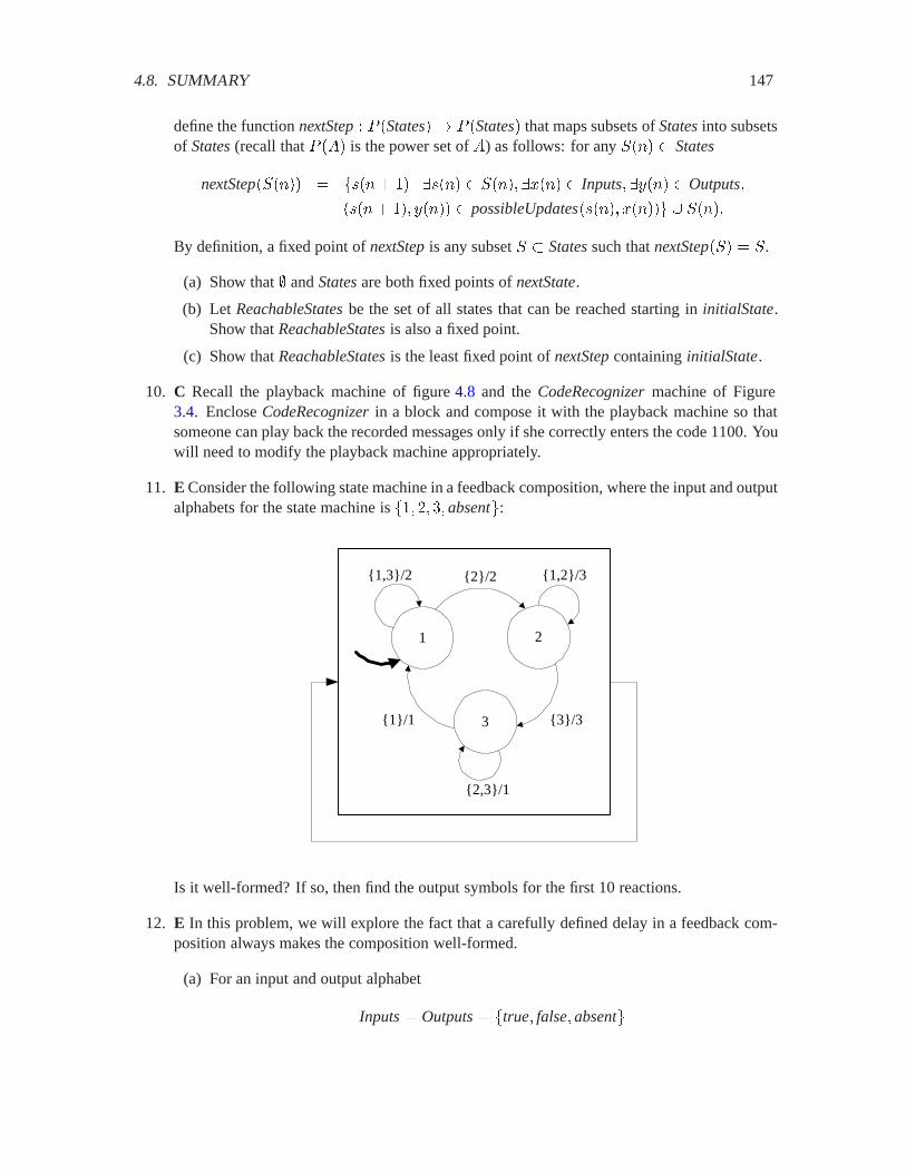
4.8. SUMMARY 147
define the function nextStep� � �States�� � �States� that maps subsets of Statesinto subsetsof States(recall that � ��� is the power set of �) as follows: for any .��� � States
nextStep�.���� � ����� � � ����� .��������� Inputs������ Outputs�
����� �� ����� possibleUpdates������ ����� � .����
By definition, a fixed point of nextStepis any subset . � Statessuch that nextStep�.� � ..
(a) Show that � and Statesare both fixed points of nextState.
(b) Let ReachableStatesbe the set of all states that can be reached starting in initialState.Show that ReachableStatesis also a fixed point.
(c) Show that ReachableStatesis the least fixed point of nextStepcontaining initialState.
10. C Recall the playback machine of figure 4.8 and the CodeRecognizermachine of Figure3.4. Enclose CodeRecognizerin a block and compose it with the playback machine so thatsomeone can play back the recorded messages only if she correctly enters the code 1100. Youwill need to modify the playback machine appropriately.
11. E Consider the following state machine in a feedback composition, where the input and outputalphabets for the state machine is �� �� ��absent:
1 2
{2}/2
{3}/3
{1,3}/2 {1,2}/3
3{1}/1
{2,3}/1
Is it well-formed? If so, then find the output symbols for the first 10 reactions.
12. E In this problem, we will explore the fact that a carefully defined delay in a feedback com-position always makes the composition well-formed.
(a) For an input and output alphabet
Inputs� Outputs� �true� false�absent

148 CHAPTER 4. COMPOSING STATE MACHINES
design a state machine that outputs falseon the first reaction, and then in subsequentreactions, outputs the value observed at the input in the previous reaction. This is similarto UnitDelayof problem 5 at the end of chapter 3, with the only difference being that itoutputs an initial falseinstead of absent.
(b) Compose the machine in figure 4.14 (b) with the delay from part (a) of this problem in afeedback loop (as in figure 4.16). Give an argument that the composition is well-formed.Then do the same for figure 4.14 (c) instead of (b).
13. C Construct a feedback state machine with the structure of figure4.12 that outputs the peri-odic sequence �� �� !� �� �� ! (with, as usual, any number of intervening stuttering outputsbetween the non-stuttering outputs).
14. E Modify figure 4.1 as necessary so that the machines in the side-by-side composition areboth nondeterministic.
15. E Modify figure 4.3 as necessary so that the machines in the cascade composition are bothnondeterministic.
16. C,T Data packets are to be reliably exchanged between two computers over communicationlinks that may lose packets. The following protocol has been suggested. Suppose computer� is sending and � is receiving. Then � sends a packet and starts a timer. If � receives thepacket it sends back an acknowledgment. (The packet or the acknowledgment or both maybe lost.) If � does not receive the acknowledgment before the timer expires, it retransmits thepacket. If the acknowledgment arrives before the timer expires, � sends the next packet.
(a) Construct two state machines, one for � and one for �, that implement the protocol.
(b) Construct a two-state nondeterministic machine to model the link from � to �, andanother copy to model the link from � to �. Remember that the link may correctlydeliver a packet, or it may lose it.
(c) Compose the four machines to model the entire system.
(d) Suppose the link correctly delivers a packet, but after a delay that exceeds the timersetting. What will happen?
17. T Consider the following three state machines:
a b
{1}/0 {1}/0{0}/ 0
{0}/1
machine A
c d
{1, 0}/1 {0}/0
{1}/0
e
{1}/0
machine B

4.8. SUMMARY 149
machine A machine B
machine C
Machines � and � have input and output alphabets
Inputs� Outputs� �� �absent�
Machine � has the same output alphabet, but input alphabet Inputs� � �react�absent.(a) Which of these machines is deterministic?
(b) Draw the state transition diagram for the composition (machine C), showing only statesthat are reachable from the initial state.
(c) Give the Behaviors� relation for the composition of machine C, ignoring stuttering.
18. T The feedback composition in figure 4.14(c) is ill-formed because it has two non-stutteringfixed points in each of the two states of the component machine. Instead of declaring it to beill-formed, we could have interpreted the composition as representing a nondeterministic statemachine. That is, in each state, we accept either of the two possible fixed points as possiblereactions of the machine. Using this interpretation, give the nondeterministic machine for thefeedback composition by giving its sets and functions model and a state transition diagram.

150 CHAPTER 4. COMPOSING STATE MACHINES
Chapter 5
Linear Systems
Recall that the state of a system is a summary of its past. It is what the system needs to rememberabout the past in order to react at the present and move into the future. In previous chapters, systemstypically had a finite number of possible states. Many useful and interesting systems are not likethat, however. They have an infinite number of states. The analytical approaches used to analyzefinite-state systems, such as simulation and bisimulation, get more difficult when the number ofstates is not finite.
In this chapter, we begin considering infinite-state systems. We impose two key constraints. First,we require that the state space and input and output alphabets be numeric sets. That is, we must beable to do arithmetic on members of these sets. (Contrast this with the answering machine example,where the states are symbolic names, and no arithmetic makes sense.) Second, we require that theupdatefunction be linear. We will define what this means precisely. In exchange for these twoconstraints, we gain a very rich set of analytical methods for designing and understanding systems.In fact, most of the remaining chapters are devoted to developing these methods.
In particular, we study state machines with
States � Reals�
Inputs � Reals� (5.1)
Outputs � Reals� �
Such state machines are shown schematically in figure 5.1. The inputs and outputs are in productform, as discussed for general state machines in section 4.4. The system, therefore, can be viewedas having 3 distinct inputs and > distinct outputs. So the input is a tuple with 3 real numbers,and the ouptut is a tuple with > real numbers. Such a system is called a multiple-input, multiple-output system, or MIMO system. When 3 � > � , it is called a single-input, single-outputsystem, or SISO system. The state is a tuple with � real numbers. � (rather than 3 or >) iscalled the dimension of the system.
Example 5.1: A stereo audio system processes two channels of audio, and therefore
151
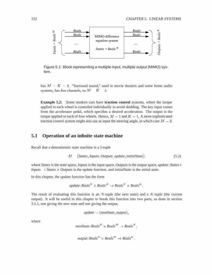
152 CHAPTER 5. LINEAR SYSTEMS
MIMO differenceequation system
States = Reals N
Reals
Reals
Reals
...
Reals
Reals
Reals
...
Ou
tpu
ts =
Re
als
K
Inp
uts
= R
ea
ls M
Figure 5.1: Block representing a multiple-input, multiple output (MIMO) sys-tem.
has 3 � > � �. ”Surround sound,” used in movie theaters and some home audiosystems, has five channels, so 3 � > � �.
Example 5.2: Some modern cars have traction control systems, where the torqueapplied to each wheel is controled individually to avoid skidding. The key input comesfrom the accelerator pedal, which specifies a desired acceleration. The output is thetorque applied to each of four wheels. Hence, 3 � and > � �. A more sophisticatedtraction control system might also use as input the steering angle, in which case 3 � �.
5.1 Operation of an infinite state machine
Recall that a deterministic state machine is a 5-tuple
3 � �States� Inputs�Outputs�update� initialState� (5.2)
where Statesis the state space, Inputsis the input space, Outputsis the output space, update�States�Inputs� States�Outputsis the update function, and initialStateis the initial state.
In this chapter, the updatefunction has the form
update�Reals� � Reals� � Reals� � Reals� �
The result of evaluating this function is an � -tuple (the next state) and a >-tuple (the currentoutput). It will be useful in this chapter to break this function into two parts, as done in section3.1.1, one giving the new state and one giving the output,
update� �nextState�output��
wherenextState�Reals� � Reals� � Reals� �
output�Reals� � Reals� � Reals� �
5.1. OPERATION OF AN INFINITE STATE MACHINE 153
such that
� � Reals� ��� Reals� � update��� �� � �nextState��� ���output��� ����
These two functions separately give the next state and the current output as a function of the currentstate and input. Given an input sequence ���� ���� of 3 -tuples in Reals� , the system recur-sively generates a state response ���� ���� of � -tuples in Reals� and an output response���� ���� of >-tuples in Reals� as follows:
��� � initialState�
����� �� ����� � update������ ������ � � � (5.3)
The second equation can be rewritten as a separate state update equation,
� � Integers� � � � ���� � � nextState������ ����� (5.4)
and an output equation,
� � Integers� � � � ���� � output������ ������ (5.5)
Equations (5.4) and (5.5) together are called a state-space model of the system, because instead ofgiving the output directly as a function of the input, the state is explicitly described. The equationssuggest a detailed procedure for calculating the response of a system. We start with a given initialstate ��� � initialState, and an input sequence ���� ���� . At step � � , we evaluate theright-hand side of (5.4) at the known values of ���� ��� and we assign the result to ���. At step� � , we evaluate the right-hand side at the known values of ���� ��� and we assign the resultto ����. To proceed from step � to step � � , we only need to remember ���� and know thenew input ����. At each step �, we evaluate the output ���� using (5.5). This procedure is nodifferent from that used for state machines in previous chapters. However, starting with section5.2,we will specialize the nextStateand outputfunctions so that they are linear, which will then lead toa powerful set of analytical tools.
5.1.1 Time
The index � in the equations above denotes the step number, the count of reactions, as with anystate machine. For general state machines, it is rare to associate a fixed time interval with a step.So there is normally no simple relation between the step number and the real time at which thecorresponding reaction occurs. For example, in the answering machine, if the initial state is idle,there may be an arbitrary amount of time before ring occurs and the state moves to count1.
The systems we study in this and the next several chapters, however, usually evolve with a fixedtime interval between updates. Suppose this interval is Æ seconds. Then step � occurs at time �Æseconds, relative to time 0. Such systems are discrete-time systems, and the index � is called thetime index.
We will require that for each time index �, the input ���� be in Reals� and the output ���� be inReals� . We disallow stuttering input or output values such as absent. This is consistent with theinterpretation of � as a real (physical) time index: the system’s input and output must take somephysical value at each �, and absentis not such a value.

154 CHAPTER 5. LINEAR SYSTEMS
Basics: Functions yielding tuples
The ranges of the nextStateand output functions are tuples. It will help to un-derstand their role if we break them down further into an � -tuple and >-tuple offunctions, one for each element of the result tuple. That is, we define the functions
nextState��Reals� � Reals� � Reals� & � � � ��
such that � � Reals� ��� Reals� ,
nextState��� �� � �nextState���� ��� �nextState� ��� ����
We write simply
nextState� �nextState�� �nextState� ��
The output function can be given similarly as
output� �output�� �output���
whereoutput��Reals� � Reals� � Reals� & � � �>�
Using these, the state update equation and output equation can be written asfollows. For all � Integers, � � ,
����� � � nextState��������� � �� ����� ������� � �� ������
����� � � nextState��������� � �� ����� ������� � �� ������
(5.6)
�� ��� � � nextState� �������� � �� ����� ������� � �� ������
and
����� � output��������� � �� ����� ������� � �� ������
����� � output��������� � �� ����� ������� � �� ������
(5.7)
����� � output��������� � �� ����� ������� � �� ������
This system of equations shows the detailed structure of the operation of such astate machine.
5.2. LINEAR FUNCTIONS 155
Example 5.3: Compact discs store digital audio signals as discrete-time signals. Foreach channel of audio, there are 44,100 numbers (samples) representing each secondof sound. The �-th number, therefore, represents the sound value at time �Æ from thebeginning of the CD, where Æ � ���� , about 23 microseconds. By contrast, thetelephone network transmits speech signals by sending only 8,000 samples per second,so the sampling interval is Æ � ��� , or 125 microseconds. We will see in chapter11 that this difference (partly) accounts for the lower audio quality over the telephonenetwork, compared to CDs.
The systems in this chapter will be time-invariant systems, meaning that the nextStateand outputfunctions do not change with the time index �. It is, therefore, a matter of convention to have timestart at 0 rather than, say, at -10 or 50. We will stick to convention and so the set of input signals inthis chapter will be
InputSignals� �Integers� � Reals� ��
where Integers� � Naturals� � �� � �� . Correspondingly,
OutputSignals� �Integers� � Reals� ��
The state response, then, is a function
�� Integers� � Reals�
where ��� � initialState.
5.2 Linear functions
A function � �Reals� Realsis a linear function if �0 Realsand � Reals,
���0� � ���0��
and �0� " Reals,��0� "� � ��0� � ��"��
The first property is called homogeneity and the second property is called additivity. When itsdomain and range both are Reals, a linear function can be represented as
�� Reals� ���� � ��� (5.9)
for some constant �. The term “linear” comes from the fact that the graph of this function is a straightline through the origin, with slope �. (If the line did not pass through the origin, the function is saidto be affine. It would satisfy neither homogeniety nor additivity.) We need a more general notionof linear function, one that operates on tuples.
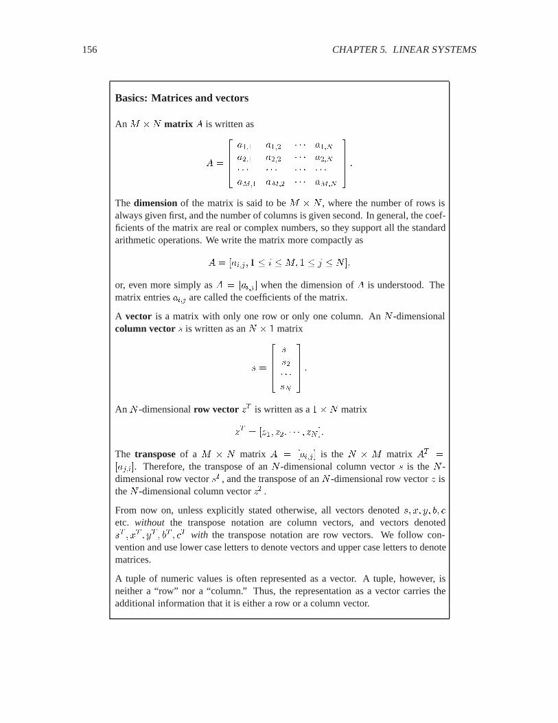
156 CHAPTER 5. LINEAR SYSTEMS
Basics: Matrices and vectors
An 3 �� matrix � is written as
� �
��������� ���� �������� ���� ���� ���� ���� ����
����� �
The dimension of the matrix is said to be 3 � � , where the number of rows isalways given first, and the number of columns is given second. In general, the coef-ficients of the matrix are real or complex numbers, so they support all the standardarithmetic operations. We write the matrix more compactly as
� � ����� � � & �3� � � � ��
or, even more simply as � � ������ when the dimension of � is understood. Thematrix entries ���� are called the coefficients of the matrix.
A vector is a matrix with only one row or only one column. An � -dimensionalcolumn vector � is written as an � � matrix
� �
�����
���� ��
����� �
An � -dimensional row vector �� is written as a �� matrix
�� � ���� ��� � �� ��
The transpose of a 3 � � matrix � � ������ is the � � 3 matrix �� �������. Therefore, the transpose of an � -dimensional column vector � is the � -dimensional row vector �� , and the transpose of an � -dimensional row vector � isthe � -dimensional column vector �� .
From now on, unless explicitly stated otherwise, all vectors denoted �� �� �� �� !etc. without the transpose notation are column vectors, and vectors denoted�� � �� � �� � �� � !� with the transpose notation are row vectors. We follow con-vention and use lower case letters to denote vectors and upper case letters to denotematrices.
A tuple of numeric values is often represented as a vector. A tuple, however, isneither a “row” nor a “column.” Thus, the representation as a vector carries theadditional information that it is either a row or a column vector.

5.2. LINEAR FUNCTIONS 157
Basics: Matrix arithmetic
Two matrices (or vectors, since they are also matrices) can be added or subtractedprovided that they have the same dimension. Just as with adding or subtractingtuples, the elements are added or subtracted. Thus if � � ������ and � � ������ andboth have dimension 3 �� , then
��� � ����� � ���� ��
Under certain circumstances, matrices can also be multiplied. If � has dimension3 �� and � has dimension � �� , then the product �� is defined. The numberof columns of � must equal the number of rows of �. Suppose the matrices aregiven by
� �
��������� ���� �������� ���� ���� ���� ���� ����
����� � � �
��������� ���� �������� ���� ���� ���� ���� ����
����� �
Then the &� element of the product � � �� isa
!��� ���
���
�������� � (5.8)
The product � has dimension 3 � � .
Of course, matrix multiplication also works if one of the matrices is a vector. If �is a column vector of dimension � , then ! � �� as defined by (5.8) is a columnvector of dimension 3 . If on the other hand �� is a row vector of dimension 3 ,then !� � ��� as defined by (5.8) is a row vector of dimension � .
Multiplying a matrix by a vector can be interpreted as applying a function to atuple. The vector is the tuple and the matrix (together with the definition of matrixmultiplication) defines the function. Thus, in introducing matrix multiplication intoour systems, we are doing nothing new except introducing a more compact notationfor defining a particular class of functions.
A matrix � is a square matrix if it has the same number of rows and columns.A square matrix may be multiplied by itself. Thus, �� for some integer � 2 isdefined to be �multiplied by itself � times. �� is defined to be the identity matrix,also written � , which has ones along the diagonal and zeros everywhere else. If �has an inverse, then that inverse is denoted ���, and ���� � ���� � � .
aIf this notation is unfamiliar, see box on page 63.
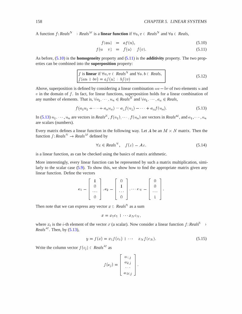
158 CHAPTER 5. LINEAR SYSTEMS
A function � �Reals� � Reals� is a linear function if �0� " Reals� and �� Reals,
���0� � ���0�� (5.10)
��0� "� � ��0� � ��"�� (5.11)
As before, (5.10) is the homogeneity property and (5.11) is the additivity property. The two prop-erties can be combined into the superposition property:
� is linear if �0� " Reals� and ��� � Reals����0� �"� � ���0� � ���"�
(5.12)
Above, superposition is defined by considering a linear combination �0� �" of two elements 0 and" in the domain of � . In fact, for linear functions, superposition holds for a linear combination ofany number of elements. That is, �0�� � 0� Reals� and ���� � �� Reals,
����0� � � ��0�� � ����0�� � � ����0��� (5.13)
In (5.13) 0�� � 0� are vectors in Reals� , ��0��� � ��0�� are vectors in Reals� , and ��� � ��are scalars (numbers).
Every matrix defines a linear function in the following way. Let � be an 3 �� matrix. Then thefunction � �Reals� � Reals� defined by
�� Reals� � ���� � ��� (5.14)
is a linear function, as can be checked using the basics of matrix arithmetic.
More interestingly, every linear function can be represented by such a matrix multiplication, simi-larly to the scalar case (5.9). To show this, we show how to find the appropriate matrix given anylinear function. Define the vectors
�� �
�����
����� � �� �
�����
����� � �� �
�����
����� �
Then note that we can express any vector � Reals� as a sum
� � ���� � ���� �where �� is the &-th element of the vector � (a scalar). Now consider a linear function � �Reals� �Reals� . Then, by (5.13),
� � ���� � ������� � � ������ �� (5.15)
Write the column vector ����� Reals� as
����� �
�����
�������� ����
����� �
5.2. LINEAR FUNCTIONS 159
Then we can rewrite (5.15) as
� �
�����
���� ��
����� � ��
�����
�������� ����
������ ��
�����
�������� ����
������ � ��
�����
�������� ����
�����
�
��������� ���� �������� ���� ���� ���� ���� ����
����������
���� ��
����� �
More compactly,
� � ���
where � is the 3 �� matrix
� � ����� � � & �3� � � � ��
Thus, there is a straightforward association between linear functions with domain Reals� and rangeReals� and 3 �� matrices. This association will be very important for us.
Example 5.4: The function ��Reals� � Realsgiven by
�� Reals�� ����� ��� ��� � ���� � ����
is linear, as can be checked by verifying (5.12). Here, �� refers the the &-th element ofthe vector �. The matrix representation is
���� � ���� � ������� ������
��� �
The function � �Reals� � Reals� given by
�� Reals� � ����� �
������ if � ) ���� if � � �
�
is linear. Here ����� refers to the �-th element of the vector ����. The matrix repre-sentation is
���� �
�����
����� ��

160 CHAPTER 5. LINEAR SYSTEMS
5.3 The ��������� representation of a discrete linear system
We consider an arbitrary system with
States� Reals� � Inputs� Reals� � Outputs� Reals� �
Its state-space model is given by the state update and output equations: �� Integers�,
���� � � nextState������ ������
���� � output������ ������
This system is said to be a linear system if the initial state is an � -tuple of zeros, and the nextStateand output functions are linear. If it is also time invariant (the nextStateand output functions donot change with time), then we have a linear time-invariant system, or LTI system. We can thenrepresent the nextStatefunction by a �����3� matrix and the outputfunction by a >����3�matrix.
Consider the � � �� �3� matrix representing the nextStatefunction. This matrix has � �3columns. We denote the ��� matrix comprising the first � columns by �, and the ��3 matrixcomprising the last 3 columns as �, so that
nextState������ ����� � ����� �������
We similarly partition the > � �� �3� matrix representing the output function into the > � �matrix � comprising the first � columns and the >�3 matrix � comprising the last 3 columns.Then
output������ ����� � ����� �������
With this notation, the state-space model is represented as
���� � � ����� �������
���� � ����� �������(5.16)
This is the ��������� representation of the LTI system. This compact representation is verypowerful. All the results in this chapter and the next are in terms of these four matrices. The� matrix is the most important, since it characterizes the system dynamics as we will see in thesections below.
Example 5.5: Take ��������� as
� �
���
��� � � �
���
��� �
� ��
�� � �
���

5.3. THE ��������� REPRESENTATION OF A DISCRETE LINEAR SYSTEM 161
So � � ��3 � �> � . (This is a 3-dimensional, SISO system.) Using these in(5.16) gives the state-space model in tuple form,
����� � � ����� � ������
����� � � ����� � ������
����� � � ����� � �����
���� � ����� � �����
The first three equations together give the nextStatefunction, the fourth equation givesthe outputfunction.
Observe in (5.16) that if initialState is zero, ��� � , and the input ���� � , for all � � , thenthe state is unchanged, ���� � . That is why we say that 0 is an equilibrium or rest state of the��������� system.
Example 5.6: An echo effect can be obtained for audio signals by realizing the fol-lowing difference equation,
���� � ���� � *�������
where the (discrete-time) audio input is �, the output is �, � * ) is a real constant,and � Naturals is an integer constant. Together, * and � determine how long theecho lasts and what it sounds like. Once again, this is a SISO system, with 3 ��> � . This works simply because the output sample at � is a combination of thecurrent input ���� and a scaled old output *������, called the echo term. Typically,� needs to be a large number to hear this as an echo. For example, if the sample rate is�� samples per second, then if � � �, the echo term *������ is the previousoutput one second earlier. This will be heard as a distinct echo.
To construct a state-space model, we need to figure out what will work as the state.Since the output depends on ������, which is past history, the state will have to yield������. The following state definition will work,
���� �
��������� ����� �� ������
����� �
It is easy to check that with this state definition, ��������� are given by
� �
����������
* ...
......
......
����������� � �
������
...
������ �
� �� *
�� � �
���

162 CHAPTER 5. LINEAR SYSTEMS
5.3.1 Impulse response
The ��������� representation provides a complete description of an LTI system. It is a completein the sense that given any input sequence, we can calculate the output sequence using the state andoutput equations of (5.16) (or (5.19) and (5.20) for the scalar case). We will discover that thereare several other descriptions of LTI systems that are also complete. The first of these that we willconsider is the impulse response. For systems that are initially at rest, the impulse response givesenough information to calculate the output sequence given any input sequence. The calculation isperformed using what is known as a convolution sum.
Suppose that 3 � , and the input sequence � is given by � � Æ, where
� � Integers� ��� �
�� if � � � if � ��
� (5.17)
This function � Integers� Realsis called an impulse, or a Kronecker delta function (this func-tion figures prominently in chapters 8 and 9). Remarkably, the response of an LTI system to thisparticular input is a complete description of the LTI system.
Assuming the system is initially at rest, we can use (5.16) to write the state response to input Æ as
��� �
��� � �
���� � ��
���� � ���
���� � �����
This is because if � � Æ, then ��� � and ���� � for all � �� .
To avoid confusion, we will use the name � instead of � for the output of a system when the input isthe impulse Æ. In other words, while � is the output for any input �, � is the output for the specificinput Æ. This output is called the impulse response. Using (5.16), it can be written as
��� � �
��� � ��
���� � ���
���� � ����
���� � ������
Of course, since the system is initially at rest, ���� � for all � ) . We can recognize the pattern

5.3. THE ��������� REPRESENTATION OF A DISCRETE LINEAR SYSTEM 163
and write the impulse response as
� � Integers� ���� �
����
� if � ) �� if � � ������� if � �
� (5.18)
This formula is rarely the right way to compute an impulse response (usually it is easier to directlydetermine the output when the input is an impulse), but it does relate the impulse response to the��������� representation. The remarkable fact, developed below, is that knowing the impulseresponse is sufficient to calculate the output given any input (assuming the system is initially atrest).
The impulse response only makes sense if the dimension 3 of the input is one (otherwise the inputcould not be an impulse as defined above). We can gain insight by considering even more specialsystems where � � > � , as done in the next section.
5.3.2 One-dimensional SISO systems
The simplest LTI system is the one-dimensional, single-input, single-output (SISO) system. Since� � 3 � > � , the ��������� representation is simply ��� �� !� �� where �� �� !� � are scalarconstants. The state-space model (5.16) is �� Integers�,
���� � � ����� � ������ (5.19)
���� � !���� � ������ (5.20)
The initial state ��� � initialState. For this system, the state at a given time index is a real number,as are the input and the output.
Let us consider an example where we construct a state-space model from an input-output descriptionof a system.
Example 5.7: In section 2.3.3 we considered a simple moving average example,where the output � is given in terms of the input � by
� � Integers�� ���� � ����� � ���� ����� (5.21)
This is not a state-space model because it gives the output directly in terms of thecurrent and pastinput. To construct a state-space model for it, we first need to decidewhat the state is. Usually, there are multiple answers, so we face a choice. The state isa summary of the past. Examining (5.21), it is evident that we need to remember theprevious input, ��� � �, in order to produce an output ���� (of course, we also needthe current input, ����, but that is not part of the past; that is the present). So we candefine the state to be
� � Integers�� ���� � ���� ��
164 CHAPTER 5. LINEAR SYSTEMS
We assume that the system is initially at rest, i.e., ��� � . (If we knew ����, wewould take that to be the initial state.) With this choice of state, we need to choose �,�, !, and � so that (5.19) and (5.20) are equivalent to (5.21). Let us look first at (5.20),which reads
���� � !���� � ������
Observing that ���� � �����, can you determine ! and �? From (5.21), it is obviousthat ! � � � ��.
Next, we determine � and � in
���� � � ����� � ������
Since ���� � ���� �, it follows that ���� � � ����, and this becomes
���� � ����� � � ������
from which we can see that � � and � � .
Note that we could have chosen the state differently. For example,
� � Integers�� ���� � ���� ���
would work fine. How would that change �, �, !, and �? (The fact that differentchoices of state can give the same input-output relation is connected with the notion ofbisimulation in section 3.4.)
In the preceding example, we started with an input-output description and obtained a state-spacemodel. The next example shows we can also go the other way.
Example 5.8: Consider a one-dimensional SISO system
���� � � ����� � ������
���� � !���� � ������
From these equations we get
���� � !������ � � ����� �� � ������
���� � � !���� � � ����� ��
Multiplying the second equation by � and subtracting from the first eliminates the stateto yield a difference equation description of the system,
����� ����� � � ����� � �!�� ������� ��
There is a generalization of this example that works for state-space models of anydimension.
In the following example, we use a state-space model to calculate the output of a system given aninput sequence.
5.3. THE ��������� REPRESENTATION OF A DISCRETE LINEAR SYSTEM 165
Example 5.9: Suppose the state ���� is your bank balance at the beginning of day �,and ���� is the amount you deposit or withdraw during day �. If ���� 2 , it meansthat you are making a deposit of ���� dollars, and if ���� ) , it means that you arewithdrawing ���� dollars. The output of the system at time index � is the bank balanceon day �. Thus,1
States� Inputs� Outputs� Reals�
Suppose that the daily interest rate is �. Then your balance at the beginning of day ��is given by
� � Integers� ���� � � � � ������ � ����� (5.22)
The output of the system is your current balance,
� � Integers� ���� � �����
Comparing to (5.19)-(5.20), we have � � � �, � � , ! � , and � � . The initialcondition is initialState, your bank balance at the beginning of day 0. Suppose the dailyinterest rate is 0.01, or one percent.2 Suppose that initialState� , and you deposit� dollars on day 0 and withdraw � every subsequent day for the next 30 days.What is your balance ���� on day 31?
You can compute ���� recursively from
��� � �
��� � ���� � �
���� � � ����� � �� � � � � ��
but this would be tedious. We can instead develop a formula that is a bit easier to use.We will do this for a general one-dimensional ��� �� !� �� system.
Suppose we are given an input sequence ���� ���� for an ��� �� !� �� system. As in example5.9,if we repeatedly use (5.19) we obtain the first few terms of a sequence,
��� � initialState� (5.23)
��� � ���� � �����
���� � ���� � ���� (5.24)
� ������ � ���� � ����
� ����� � ����� � �����
���� � ����� � ����� (5.25)
� ������� � ����� � ���� � �����
� ����� � ������ � ����� � ������
(5.26)1These sets are probably not, strictly speaking, equal to Reals, since deposits and withdrawals can only be a whole
number of cents. Also, most likely, the bank will round your balance to the nearest cent. Thus, our model here is anapproximation. Using Realsis a considerable simplification.
2 This would only be reasonable in an economy with hyperinflation.
166 CHAPTER 5. LINEAR SYSTEMS
From this it is not difficult to guess the general pattern for the state response and the output response.The state response of (5.19) is given by
���� � ��initialState��������
���������'� (5.27)
for all � � , and the output response of (5.20) is given by
���� � !��initialState��
�������
!���������'�
� ����� (5.28)
for all � � .
We use induction to show that these are correct. Induction is where we show that these are correctfor some fixed �, and then show that if it is correct for any �, then it is correct for ��. For � � ,(5.27) gives ��� � ��initialState� initialState, which matches (5.23), and hence is correct.3 Nowsuppose that the right-hand side of (5.27) gives the correct value of the response for some � � .We must show that it gives the correct value of the response for � � . From (5.19) and using thehypothesis that (5.27) is the correct expression for ����, we get
���� � � ����� � �����
� ����initialState��������
���������'�� �����
� ����initialState��������
�������'� � �����
� ����initialState���
���
�������'��
which is the expression on the right-hand side of (5.27) for � � . It follows by induction that theresponse is indeed given by (5.27) for all � � . The fact that the output response is given by (5.28)follows immediately from (5.20) and (5.27).
Example 5.10: We use formula (5.27) in example 5.9 to figure out the monthlypayment of / on a $10,000, 32-month loan with a monthly interest of �. So in(5.27) we substitute � � ��� � � �� � � , ��� � �� � ����� � , and��� � � ���� � /, to get
� ���� � ����
���
�����/�
Using the identity (valid for ? �� )
�����
?� �?��� �
?� �
3For any real number �, �� � � by definition of exponentiation.

5.3. THE ��������� REPRESENTATION OF A DISCRETE LINEAR SYSTEM 167
we get���
���
�����/ ���� �
�/�
So the monthly payment is
/ � � � � ���
��� � � � ���
In the next example we identify the unknown parameter � of an ��� �� !� �� representation giveninput-output data.
Example 5.11: Financial analysts compare alternative investment opportunities usinga measure called the internal rate of return. Suppose an investment of $10,000 atthe beginning of year 0 yields an income stream of $2,000 for each of 10 successiveyears, and nothing thereafter. By definition, the investment’s internal rate of return isthe annual interest rate � that a bank should give so that you can get the same incomestream. So we need to find � such that
���� � � � � ������ � �����
with ��� � � , ��� � , and ��� � � ���� � ��. We recognize thisas a state update with � � � � and � � . Substituting in (5.27) gives
� � � ���� ���
���
� � ����� � �
� � � ���� � � � ���� �
�� ��
so� � � ����� � ���
which we can solve by trial-and-error to obtain � � �� or 15 percent. Suppose there isanother investment opportunity for the same $10,000 investment that yields an internalrate of return smaller than 15 percent. Then, all else being equal, one would choose thefirst opportunity.
5.3.3 Zero-state and zero-input response
The expressions (5.27) for the state response and (5.28) for the output are each the sum of two terms.The role of these two terms will be better understood if we consider them in isolation.
If the system is initially at rest, initialState� , the first term vanishes, and only the second term isleft. This second term is called the zero-state response. It gives the response of the system to aninput sequence when the initial state is zero. For many applications, particularly when modeling aphysical system, the zero-state response is what we are interested in.
168 CHAPTER 5. LINEAR SYSTEMS
If the input sequence is zero, i.e. � ��� � ��� � , the second term vanishes, and only thefirst term is left. The first term is called the zero-input response. It gives the response of the systemto some initial condition, with zero input stimulus applied. Of course, if the system is initially at restand the input is zero, then the state remains at zero. So the zero-input response is only interesting ifthe system is not initially at rest.
So the right-hand side of both equations (5.27) and (5.28) are a sum of a zero-state response and azero-input response. To make it clear which equation we are talking about, we use the followingterminology:
zero-state state response The state sequence ���� when the initial state is zero.zero-input state response The state sequence ���� when the input is zero.zero-state output response The output sequence ���� when the initial state is zero.zero-input output response The output sequence ���� when the input is zero.
Note that “zero-state” really means that the initial state is zero, while “zero input” means that theinput is alwayszero.
Let us focus on the zero-state output response. First, note from (5.18) that in this scalar case, theimpulse response can be written
� � Integers� ���� �
����
� if � ) �� if � � !������ if � �
� (5.29)
We can use this sequence in (5.28) to simplify its form. This simplified form will show us how tocalculate the response to an arbitrary input given only the response to an impulse.
Combining (5.28) and (5.29), the zero-state output response can be written as
� � � � ���� ���
���
����'���'�� (5.30)
Thus, we see that � is a complete description of the system, in the sense that it is all we need toknow to find the output given any input � (assuming zero initial state).
Let ���� � for all � ) , and, noting that ���� � for all � ) , we can write this as
� � Integers� ���� ���
��������'���'�� (5.31)
The additional terms in the summation are harmless because they all have value zero. A summationof this form is called a convolution sum. We say that � is the convolution of � and �, and write itusing the shorthand
� � � � �.
The ‘*’ symbol represents convolution. By changing variables, defining 6 � � �', one can seethat the convolution sum can also be written in the equivalent form
� � Integers� ���� ���
������6����� 6�� (5.32)

5.3. THE ��������� REPRESENTATION OF A DISCRETE LINEAR SYSTEM 169
-5 0 5 100
0.2
0.4
0.6
0.8
1
n
x
-5 0 5 100
0.5
1
1.5
2
2.5
n
s
Figure 5.2: Plots of the impulse (left) and the impulse response of example5.12 (right) for � � �.
That is, � � � � � � �. Convolution sums will be studied in much more detail in chapter9.
The impulse response of a system is simply the output when the input is an impulse.If the system is initially at rest, then its output is given by the convolution of theinput and the impulse response.
Example 5.12: For our bank example, � � � �, � � , ! � , and � � in (5.20).The impulse response of the bank system is given by (5.18),
���� �
�� if � � � � ������ if � �
�
This represents the balance of a bank account with daily interest rate � if an initialdeposit of one dollar is put in on day 0, and no further deposits or withdrawals are made.Notice that since � � 2 , the balance continues to increase forever; see figure5.2.This system is said to be unstable because even though the input is always bounded,the output grows without bound. The system is also an infinite impulse response (IIR)system.
Writing the output as a convolution, using (5.30), we see that
� � � � ���� ��������
� � ���������'��
This gives a simple formula that we can use to calculate the bank balance on any givenday (although it will be tedious for large �, and you will want to use a computer).
The zero-input state response of the ��� �� !� �� system is
���� � ������ � � �
170 CHAPTER 5. LINEAR SYSTEMS
This is a geometric or exponential sequence. If ��� �� , the response will eventually die out, i.e.����� as ���, if and only if ��� ) , in which case we say the system is stable.
5.3.4 Multidimensional SISO systems
In the previous section we considered the simplest systems of the form of figure5.1 with 3 � > �� � . Systems with larger dimension, � 2 , occur more frequently in practice. In this section,we allow the dimension � to be arbitrarily large, but keep the simplification that 3 � > � ,so the system is still SISO (single-input, single-output). In the ��������� representation, � is� � � , � is � � , � is � � and � is � . So for an SISO system we may write � � �,� � !� , � � �, where �� ! are � -dimensional column vectors and � is a scalar. Thus, SISOsystems have an ��� �� !� �� representation, and their state-space model is
���� � � ����� � ������ (5.33)
���� � !� ���� � ������ (5.34)
The result of evaluating the nextStatefunction (5.33) is an � -dimensional vector, ��� � �. The� �� matrix � defines the linear combination of the � elements of ���� that are used to calculatethe � elements ���� �. The � -dimensional column vector � defines the weights used to include���� in the linear combination for each element of ���� �.
The result of evaluating the outputfunction (5.34) is a scalar, ����. The � -dimensional row vector!� defines the linear combination of elements of ���� and � defines the weight used to include ����in the output ����.
Example 5.13: Above we constructed a state-space model for a length-two movingaverage. The general form of this is the 3 -point moving average, given by
� � Integers� ���� �
3
�������
���� 6�� (5.35)
To be specific, let’s take 3 � �. Equation (5.35) becomes
� � Integers� ���� �
������ � ���� � � ���� ���� (5.36)
We can construct a state-space model for this in a manner similar to what we did forthe length-two moving average. First, we need to decide what is the state. Recall thatthe state is the summary of the past. Equation (5.36) tells us that we need to remember��� � � and ��� � ��, the two past inputs. We could define these to be the state,collected as a column vector,
���� �
���� ����� ��
��
(Of course, we could have equally well put the elements in the other order; see exercise9.)

5.3. THE ��������� REPRESENTATION OF A DISCRETE LINEAR SYSTEM 171
Consider the output equation (5.34). We need to determine !� and �. The vector !� is arow vector with dimension � � �, so we must fill in the blanks in the output equationbelow:
���� � � � �
���� ����� ��
�� � �����
It is easy to see that each of the three blanks must be filled with �3 � �� in order toget (5.36). Thus,
! �
����
�� � � ���
Consider next the state equation (5.33). We need to determine � and �. The matrix �is �� �. The vector � is dimension 2 column vector. So we can fill in the blanks in theoutput equation below:
���� � �
����
���� �
��
� ���� ����� ��
��
������
From this, we can fill in the blanks, getting
� �
�and � �
��
Note that once the state is specified, there is only one way to fill in the blanks and obtainthe ��� �� !� �� representation.
The state response of the SISO system (5.33)-(5.34) is given by an expression similar to (5.27), butinvolving matrices and vectors rather than just scalars,
���� � ��initialState��������
���������'� (5.37)
for all � � . The state response is also sometimes called the state trajectory. The output responseof (5.42) is given by
���� � !���initialState� ��������
!����������'� � ����� (5.38)
for all � � . (Exercise 13 asks you to derive these equations.)
Notice again that the state response (5.37) and the output response (5.38) are each the sum of twoterms. The first term is the zero-input response and the second terms is the zero-state response.
The impulse response, in terms of the state-space model, is the sequence of real numbers
���� �
����
� if � ) �� if � � !������� if � �
(5.39)

172 CHAPTER 5. LINEAR SYSTEMS
This is just like (5.18) except that � and ! are vectors, and � is a scalar. This formula can be quitetedious to apply. It is usually easier to simply let � � Æ, the Kronecker delta function, and observe orcalculate the output. The zero-state output response is given by convolution of this impulse responsewith the input, (5.32).
Example 5.14: We can find the impulse response � of the moving average system of(5.35) by letting � � Æ, where Æ is given by (5.17). That is,
� � Integers� ���� �
3
�������
��� 6��
Now, ��� 6� � except when � � 6, at which point it equals one. Thus,
���� �
����
if � ) �3 if � � ) 3 if � �3
�
This function, therefore, is the impulse response of an 3 -point moving average system.This result could also have been obtained by comparing (5.35) to (5.32), the output as aconvolution. Or it could have been obtained by constructing a state-space model for thegeneral length-3 moving average, and applying (5.39). However, this latter methodwould have proved the most tedious in this case.
Notice that in the previous example, the impulse response is finite in extent (it starts at 0 and stopsat 3�). For this reason, such a system is called a finite impulse response system or FIR system.
Example 5.15: The 3 -point moving average can be viewed as a special case of themore general FIR system given by
� � Integers� ���� ��������
��6����� 6��
Letting ��6� � �3 for � 6 ) 3 , we get the 3 -point moving average. Choosingother values for ��6�, however, we can get other responses (this will be explored inchapter 8).
A state-space model for the FIR system is constructed by again deciding on the state.A reasonable choice is the 3 � past samples of the input,
���� � ����� �� ���� ��� � ����3 � ��� �
a column vector. The state-space model is then given by (5.33) and (5.34) with
� �
�������
������� � � �
�������
������� � ! �
�������������� ��3 � ����3 � �
������� �

5.3. THE ��������� REPRESENTATION OF A DISCRETE LINEAR SYSTEM 173
h(n)
n......
10.7
0.490.343
Figure 5.3: Impulse response of the echo example 5.16 for * � �� and � � �.
� � ����
Notice that the model that we found in example 5.13 has this form. The �3 � � ��3 � � matrix � has coefficients ������ � , while all other coefficients are zero.This is a rather special form of the � matrix, limited to FIR systems. The vector �has the first coefficient equal to 1, while all others are zero. The vector ! contains thecoefficients of the impulse response.
Many interesting systems, unlike this example, have an infinite impulse response, and are referredto as IIR systems.
Example 5.16: Recall from example 5.6 that an echo effect can be obtained for audiosignals by realizing the following difference equation,
� � Integers� ���� � ���� � *�������
The impulse response � can be obtained by simply letting the input be an impulse,� � Æ, and finding the output � � �. That is
� � Integers� ���� � ��� � *������� (5.40)
But of course, this means that
������ � ����� � *���� ����
Substituting this back into (5.40), we get
���� � ��� � *����� � *����� ����
But of course,���� ��� � ��� ��� � *���� ����
so���� � ��� � *�� ��� � *���� ��� � *����� ����
Continuing in this fashion, we see that the impulse response of the echo system is theoriginal impulse and an infinite set of echos (delayed and scaled impulses). This can bewritten compactly as follows,
� � Integers� ���� ������
*���� 6���
174 CHAPTER 5. LINEAR SYSTEMS
This impulse response is plotted in figure 5.3 for � � � and * � ��. In that figure,you can see that the original impulse gets through the system at � � , while the firstecho is scaled by �� and delayed to � � �, and the second echo is scaled by ��� anddelayed to � � �.
We can check this impulse response using the state-space representation of example5.6 in (5.39). From example 5.6, we have that � � , so (5.39) is obviously correctfor � ) and � � . Checking it for � 2 is somewhat more involved. Assuming� � �, we have from example 5.6
� �
�����
*
����� � � �
�����
����� � ! �
�����
*
����� � � �
���
To use (5.39) we need to know ����. It is easy to check that
�� �
�����
* *
����� � �� �
�����
* * *
����� � � �
�����* * * *
����� � *��
where � is the �� � identity matrix. Thus,
�� � *�� �� � *��� �� � *��� �� � *� � *���
The pattern continues. Note that because of the particular structure of �, ����� issimply the first column of ����. Thus,
��� � !���� � � *�
�����
����� � �
Similarly,
���� � !��� � � *�
�����
����� � �
and
���� � !���� � � *�
�����
����� � �
Only when we get to ���� do we get a non-zero result,
���� � !���� � � *�
�����
����� � *�
5.3. THE ��������� REPRESENTATION OF A DISCRETE LINEAR SYSTEM 175
Continuing in this fashion, we can determine that 3 of every four samples of the impulseresponse are zero, and the non-zero ones have the form *�� where � is a multiple offour, in perfect agreement with figure 5.3.
The echo system of the previous example is called an infinite impulse response (IIR) systembecause the response to an impulse never completely dies out. Here is another example of an IIRsystem.
Example 5.17: An audio oscillator is a system that produces a sinusoidal signal of agiven frequency. We can construct one with the two-dimensional system given by
� �
������ � ������������ ������
�� � �
�� ! �
�� � � �
where � is a constant that will turn out to be the oscillation frequency. It can be shown(see exercise 14) that for all � � � � ��
�� �
������� � �������������� �������
��
Suppose the initial state isinitialState� �� �� �
Then the zero-input state response is
�� !"���#����� � �� &�&&�,.��
�
������� � �������������� �������
�
�
�
� ��������������
��
and the zero-input response is
�� !"���#����� � !� �� &�&&�,.��
��
� � ��������������
�
� � ��������
Notice that without any input, as long as the initial state is non-zero, the system willproduce a sinusoidal output in perpetuity.
If we instead consider the situation where the system is initially at rest, then we findthat the impulse response is
���� �
��� if � �
!������� if � � �
176 CHAPTER 5. LINEAR SYSTEMS
For the values of �� �� ! in this example we obtain
���� �
�� if � �
� ������� ���� if � � �
Thus, if the oscillator is initially at rest, it can be started with an impulse, and its outputwill henceforth be sinusoidal, similar to the zero-input response. Thus, if the oscillatoris initially at rest, it can be started with an impulse at the input.
5.3.5 Multidimensional MIMO systems
In the preceding sections, the input and output were both scalars. A multiple-input, multiple-output (MIMO) system is only slightly more complicated. A state-space model for such a systemis
� � Integers�� ���� � � ����� ������ (5.41)
���� � ����� ������ (5.42)
where, ���� Reals� , ���� Reals� and ���� Reals� , for any integer �. In the ���������representation, � is an � �� (square) matrix, � is an � �3 matrix, � is a > �� matrix, and� is a > �3 matrix. Now that these are all matrices, it is conventional to write them with capitalletters.
Let initialState Reals� be a given initial state. Let ���� ���� ����� , be a sequence of inputsin Reals� (each input is a vector of dimension 3 ). The state response of (5.41) is given by
���� � ��initialState��������
���������'� (5.43)
for all � � , and the output sequence of (5.42) is given by
���� � ���initialState� ��������
����������'� ������ (5.44)
for all � � (each output is a vector of dimension >).
As before, the right-hand sides of these equations are the sum of a zero-input response and azero-state response. Consider the zero-state output response,
���� ��������
����������'� ������ (5.45)
for all � � . Define the sequence ���� ���� ����� of > �3 matrices by
���� �
��� if � � ������� if � �
(5.46)
5.3. THE ��������� REPRESENTATION OF A DISCRETE LINEAR SYSTEM 177
Probing further: Impulse Responses of MIMO Systems
The � function in (5.46) is not the impulse response of a MIMO system with repre-sentation ���������. However, with some care, it is possible to relate it to a setof impulse responses that characterize the system.
The system has 3 inputs and > outputs, and for each integer �, ���� in (5.46)is a > �3 matrix. Each input symbol ���� is an 3 -tuple of reals. Let �����represent the '-th element in this tuple, and let �� represent the sequence of suchelements. Similarly, let ����� represent the 6-th element of the output tuple, and�� the sequence of such outputs. Finally, let ������� represent the 6�'-th elementof the matrix ����, and let ���� represent the sequence of such elements.
The SISO system comprising the 6-th output and '-th input has impulse response����. Specifically, if �� � Æ and �#��� � for all ( �� ' and for all � Integers,then �� � ����. Thus, � can be viewed as a matrix of impulse responses, one foreach possible pairing of input and output signals.
This can no longer be called an impulse response, because the input cannot be an impulse; it has thewrong dimension (see box).
From (5.45) it follows that the zero-state output response is given by
���� ���
���
����'���'�� � � (5.47)
This is once again a convolution sum.
The &� th element of the matrix sequence ���� ���� , namely ������� ������� , is indeedthe impulse response of the SISO system whose input is �� and whose output is ��. In terms offigure 5.1, this is the SISO system obtained by setting all inputs except the th input to zero, andconsidering only the &th output. If �� denotes the th column of � and ��
� denotes the &th row of� , then ���� is the impulse response of the SISO system ����� � ��������. All these SISO systemshave the same � matrix.
5.3.6 Linear input-output function
In the systems that this chapter considers, the nextStateand output functions are linear. Recallthat a function � �� � $ is linear if (and only if) it satisfies the superposition property: for all��� �� � , and /� 0 Reals,
��/�� � 0��� � /����� � 0������
What does it mean for a systemto be linear? Recall that a system . is a function .�� � $ ,where � and $ are signal spaces. For a MIMO system, � � �Integers� Reals� �, and $ �
178 CHAPTER 5. LINEAR SYSTEMS
�Integers� Reals� �. The function . is defined by (5.44), which gives � � .���, given �. So theanswer is obvious. . is a linear system if . is a linear function. (It is an LTI system if it is alsotime invariant).
Examining (5.44), or its simpler SISO versions, (5.28) or (5.38), it is easy to see that superpositionis satisfied if initialState is zero. This is because with zero initial state, the output ���� is a linearcombination of the input samples ����. Hence, a system given by a state-space model that is initiallyat rest is a linear system. The superposition property turns out to be an extremely useful property,as we will discover in the next chapters.
5.4 Continuous-time state-space models
A continuous-time state-space model for an LTI SISO system has the form
� Reals�� ���� � ���� � �"�� (5.48)
/�� � !� ��� � �"�� (5.49)
where
� ��Reals� � Reals� gives the state response;
� ���� is the derivative with respect to time of � evaluated at Reals�;
� "�Reals� � Realsis the input signal; and
� /�Reals� � Realsis the output signal.
As with the discrete-time SISO model, � is an � � � matrix, � and ! are � � column vectors,and � is a scalar. As before, this is the ��� �� !� �� representation of the system, but the equations aredifferent.
Continuous-time systems are no longer state machines, since inputs, outputs, and state transitions donot occur at discrete instances. Nevertheless, they share many properties of discrete systems. Themajor difference between this model and that of (5.33) and (5.34) is that instead of giving new stateas a function of the input and the old state, (5.48) gives the derivative of the state. The derivative of avector � is simply the vector consisting of the derivative of each element of the vector. A derivative,of course, gives the trend of the state at any particular time. Giving a trend makes more sense thangiving a new state for a continuous-time system, because the state evolves continuously.
All of the methods that we have developed for discrete-time systems can also be developed forcontinuous-time systems. However, they get somewhat more challenging mathematically becausethe summations become integrals. We leave it to a more advanced text to explore this.
A continuous-time state-space model may be approximated by a discrete-time state-space model(see box). In fact, this approximation forms the basis for most computer simulations of continuous-time systems. Simulation of continuous-time systems is explored in labC.6.
5.4. CONTINUOUS-TIME STATE-SPACE MODELS 179
Probing further: Approximating continuous-time systems
Discrete LTI systems often arise as approximations of continuous-time systems thatare described by differential equations. Those differential equations may describethe physics. A differential equation is of the form (see for example labC.6).
� Reals� ���� � ������ "���� (5.50)
Here Realsstands for continuous time, � � Reals� Reals� is the state re-sponse, and " � Reals� Reals� is the input signal. That is, at any time , ���is the state and "�� is the input. The notation �� stands for derivative of the stateresponse � with respect to , so ��Reals� � Reals� � Reals� is a given functionspecifying the derivative of the state. Specifying the derivative of the state is simi-lar to specifying a state update. Recall that a derivative is a normalized differenceover an infinitesimally small interval. A continuous-time system can be thought ofas one where the state updates occurs in intervals that are so small that the stateevolves continuously rather than discretely.
In general, � is an � -tuple, � � ���� � �� �, where ���Reals� � Reals. Thederivative of an � -tuple is simply the � -tuple of derivatives, �� � � ���� � ��� �.We know from calculus that
���� ���
�� !��
�
��� � � ���
�
and so, if Æ 2 is a small number, we can approximate this derivative by
���� � ��� �� ���
�
Using this for the derivative in the left-hand side of (5.50) we get
��� � � ��� � ������ "���� (5.51)
Suppose we look at this equation at sample times � � � �� . Let us denote thevalue of the state response at the �-th sample time by ���� � ����, and the valueof the input at this same sample time by ���� � "���. In terms of these variables,(5.51) becomes
���� �� ���� � ������� �����
which we can write as a state update equation,
���� � � ���� � ������� ������
180 CHAPTER 5. LINEAR SYSTEMS
5.5 Summary
This chapter has begun the exploration of state machines whose state update and output functions arelinear. The number of possible states for such systems is typically infinite, so brute-force methodsthat enumerate the states will be ineffective. Instead, powerful mathematical tools leverage thelinearity of the key functions. This chapter barely begins an exploration of the very rich set of toolsthat engineers have developed for such systems. Subsequent chapters will continue that exploration.
Exercises
Each problem is annotated with the letter E, T, C which stands for exercise, requires some thought,requires conceptualization. Some of the problems require using Matlab.
1. E Use induction to obtain (5.13) as a consequence of (5.12).
2. E Use induction to show that if
� �
� �
��
then for all � � ,
�� �
�� �����
��
��
3. E Let � �Reals� � Reals� be a linear function given by � � Reals� , ���� � �� for some� �� matrix �. Give a similar definition for the composition � Æ � . Is it also linear?
4. E What would be the monthly payment in example 5.10 if the monthly interest is 0.015?Also, what would be the total payment over the 32 months?
5. E Construct a SISO state-space model for a system whose input and output are related by
� � Integers� ���� � ���� � � ���� ���
You may assume the system is initially at rest. It is sufficient to give the � matrix, vectors �and !, and scalar � of (5.33) and (5.34).
6. E The � matrix in (5.33) for a SISO system is
� �
��
Calculate the zero-input state response if
(a) the initial state is �� �� ,
(b) the initial state is �� �� ,
(c) the initial state is �� �� .

5.5. SUMMARY 181
7. E Consider the one-dimensional state-space model, � � Integers�,
���� � � ���� � �������� � ����
Suppose the initial state is ��� � � for some given constant �. Find another constant � suchthat if the first three inputs are ��� � ��� � ���� � �, then y(3) = 0. Note: In general,problems of this type are concerned with controllability. The question is whether you canfind an input (in this case constrained to be constant) such that some particular condition onthe output is met. The input becomes a control signal.
8. E A SISO LTI system has the � matrix given by
� �
�
and the � vector by �� �� . Suppose that ��� � �� �� . Find the input sequence ���� ���so that the state at step 2 is ���� � �� ��� .
9. E In example 5.13, the state was chosen to be ���� � ����� �� ���� ���� . How would the��� �� !� �� representation change if the state were chosen to be
(a) ����� ��� ���� ��� ?
(b) ����� � � ���� ��� ��� � �� ���� ���� ?
10. E Suppose the � matrix of a two-dimensional SISO system is
� � @
������ � ������ �� ������ � ������ �
��
Suppose the initial state is ��� � �� �� , and the input is zero. Sketch the zero-input stateresponse for � � � � � � for the cases
(a) @ �
(b) @ � ��
(c) @ � �
11. E In this problem we further consider example5.9. As in the example, suppose initialState�, and you deposit � dollars on day 0 and withdraw � dollars every subsequent dayfor the next 30 days.
(a) Write a Matlab program to compute your bank balance ����� � � � �, and plot theresult.
(b) Use formula (5.27) to calculate your bank balance at the beginning of day 31. Thefollowing identity may prove useful:
�����
�� �� ����
� ��
where � �� .

182 CHAPTER 5. LINEAR SYSTEMS
12. E Use Matlab to calculate and plot the impulse response of the system
���� � � ����� � �����
���� � !����
for the following cases:
(a) � � �
(b) � � �
(c) � � ��
(d) � � ���
where in all cases, � � ! � and � � .
13. E Use induction to derive the SISO response expressions (5.37) and (5.38).
14. E Consider the two-dimensional system given in example5.17, which has
� �
������ � ������������ ������
��
Show that for all � � � � ��
�� �
������� � �������������� �������
��
Hint: use induction and the identities
����* � +� � ����*� ����+�� ����*� ����+�
����*� +� � ����*� ����+� � ����*� ����+�
15. E A damped oscillator is a variant of the oscillator in example 5.17, where the sinusoidalsignal decays with time. The damped oscillator is identical, except that the � matrix is givenby
� � *
������ � ������������ ������
��
where ) * ) is a constant damping factor.
(a) Find the zero-input state response and the zero-input response for the initial state
initialState� �� �� �
(b) Find the zero-state impulse response.

5.5. SUMMARY 183
16. T Consider the audio echo system in example 5.6. A more interesting effect (sometimescalled reverberation) can be obtained by simultaneously combining multiple echos. In thisproblem, consider the following difference equation, which combines two echos,
���� � ���� � *����3� � +�������
where the (discrete-time) audio input is �, the output is �, and � * ) and � + ) are constants that specify two distinct echo terms. Suppose for simplicity that 3 � � and� � �. These numbers are not large enough to yield an audible echo, but the mathematicalmodel is similar for larger numbers, so these are adequate for study. Note that the zero-stateimpulse response of this system is much more complicated than the simple echo system (tryto find it!), which accounts for a considerably more realistic echo effect.
(a) Give a state-space representation ��������� of this system.
(b) Modify the system so that the audio input has two channels (stereo), but the output isstill one channel. Combine the two input channels by adding them with equal weight.Give ���������.

184 CHAPTER 5. LINEAR SYSTEMS
Chapter 6
Hybrid Systems
This text models signals and systems as functions. To develop understanding, we study the structureof the domain and range of these functions, as well as the structure of the mapping from the domainto the range. Despite the uniformity of this approach, we have begun to evolve two distinct familiesof models. Chapters 3 and 4 structure this mapping using state machines. Chapter 5 generalizesthese state machines so that the number of possible states is infinite, and specializes them so thatthe systems are linear and time-invariant (LTI). LTI systems prove to yield to powerful analyticaltechniques, which are only hinted at in chapter 5. Chapters 7 through 11 will further develop theseanalytical techniques by structuring the system mapping using frequency-domain concepts.
The analytical methods available for LTI systems prove so compelling that we wish to apply themeven to systems that are not LTI. In fact, no real-world system is truly LTI. At a minimum, itsproperties were certainly different during the initial stages of the big bang, so it cannot be timeinvariant. More practically, systems change over time; they are turned on and off, they deteriorate,etc. Moreover, systems that behave as linear systems typically do so only over some regime ofoperation. For example, if the magnitude the inputs exceed some threshold, a real-world systemwill overload, and will no longer behave linearly. A similar effect might result when the statewanders beyond some modest range. This chapter shows how models that are only applicable someof the time can be used effectively.
In chapters 3 and 4, signals are sequences of events. Their domain is (typically) Naturals�, andtheir range is (typically) a finite and arbitrary set of symbols. The domain is not interpreted astime, but rather as indexes of a sequence. In chapters 5 and 7 through 11, the domain of signals isinterpreted as time. For continuous-time signals, the domain is either Realsor Reals�, whereas fordiscrete-time signals it is either Integersor Naturals�, but in either case, the domain is interpreted asrepresenting as advancing time. This interpretation of the domain as time is essential to the notionof frequency that is used throughout the forthcoming chapters.
Chapter 5 and this one provide a bridge between state-machine models and such time-based mod-els by developing state machine models for time-based systems. In this chapter, we build anotherbridge between these two families of models by showing that they can often be usefully combinedand used simultaneouslyin the samemodel, rather than as alternative views of a system. The re-sulting models are called hybrid systems. They are a powerful tool for understanding real-world
185

186 CHAPTER 6. HYBRID SYSTEMS
systems.
To understand the value of hybrid systems, it is useful to reflect on the relative strengths and weak-nesses of time-based models and state-machine models. Chapter5 demonstrates that state-machinemodels are more general by showing how they can be used to describe time-based models. Sincethey are more general, why not just always use state-machine models? The methods of state-machine models, such as composition by forming a product of the state spaces, simulation, andbisimulation, do not yield the depth of understanding that we will get in the subsequent chaptersfrom looking at frequency response. Why not always use frequency response? Frequency responseis a rather specialized analytical tool. It applies only to LTI systems. Most real-world systems arenot LTI, so such powerful analytical tools must be applied with careful caveats about the regime ofoperation over which they do apply.
Consider for example a home audio system. It takes data from a compact disc and converts it intoauditory stimulus. Is it LTI? Well, obviously not, since its system function changes rather drasticallywhen you turn it on and off. The acts of turning it on and off, however, seem to match well the statetransitions of a state machine. Can we come up with a model where there is a state machine withtwo states, “on” and “off,” and associated with each state there is an LTI system that describes thebehavior of the system in the corresponding mode of operation? Indeed we can. Such a model iscalled a hybrid system.
In order to get state machine models to coexist with time-based models, we need to interpret statetransitions on the time line used for the time-based portion of the system, be it continuous time ordiscrete time. In the audio system, for example, we need to associate a time with the acts of turningit on or off. The models used in chapters 3 and 4 do not naturally do this, since the signals thereare sequences of events. That is, they are functions whose domain is Naturals�, where there is notemporal association with an � Naturals�.
Recall from chapter 3 that the input and output alphabets of a state machine are required to includea stuttering element, typically denoted absent. Whenever the state machine reacts, if its input is thestuttering element, then it does not change state and its output will be the stuttering element. Thisis key to hybrid system models because it allows us to embed the state machine into a time-basedmodel. At any time where there is no interesting input event, the machine stutters.
A hybrid system combines time-based signals with sequences of events. The time-based signals areof the form �� � �, where � is some range (such as Realsor Complex), and is either Reals,Reals�, Integers, or Naturals�, depending on whether the time domain is discrete or continuousand whether the model includes a time origin. In chapters 3 and 4, the event signals had the form0�Naturals� � Symbols, where the set Symbolshas a stuttering element. For a hybrid system,however, these have to share a common time base with the time-based signals, so they have theform 0� � Symbols. Thus, events occur in time. Typically, for most , 0�� � absent, thestuttering element. The non-stuttering element is used only at those discrete values of time wherean event occurs.

6.1. MIXED MODELS 187
6.1 Mixed models
A state machine model becomes a time-based model if it reacts at all times in the time base . Thismeans that state machines and time-based models can interact as peers, sending time-based signalsto one another.
Example 6.1: Moving averages are popular on Wall Street for detecting trends in stockprices. But in using them, a key question arises: how long should the moving averagebe? A short-term moving average might detect short-term trends, while a long-termmoving average might detect long term trends. A classical method combines the twoand compares them to generate buy and sell signals. If the short-term trend is moresharply upward than the long term trend, a buy signal is generated. If the short termtrend is more sharply downward than the long term trend, a sell signal is generated.
A system implementing this moving average cross-over method is shown in figure6.1. The input is the discrete-time signal price� Integers� Realsrepresenting the clos-ing price of a stock each day. The LTI systems shortTermand longTermare both mov-ing average systems, but shortTermaverages fewer successive inputs than longTerm.The outputs of these systems are the discrete-time signals � and �. The finite state ma-chine reacts on each sample from these signals. It begins in the state short over long.The transition out of this state has the guard
������� ����� � ���� 2 �����
When this transition is taken, a buy signal is generated. The sell signal is generatedsimilarly. The plots below show the buy and sell signals generated by a (synthetic)sequence of stock prices.
This example illustrates a simple form of technical stock trading. In this extreme form,it has the controversial feature that it ignores the fundamentals of the company whosestock is being traded. It is using the stock price alone as the indicator of worth. In fact,much more sophisticated signal processing methods are used by technical stock traders,and they often do take as inputs other quantifiers of company worth, such as reportedrevenues and profits.
6.2 Modal models
In the previous section, time-based systems are combined with state machines as peers. A richerinteraction is possible with a hierarchical combination. The general structure of a hierarchical hybridsystem model is shown in figure 6.2. In that figure, there is a two-state finite state machine. Thereare some changes to the notation, however, from what was used in chapters3 and 4.
First, notice that the inputs and outputs include both event signals and time-based signals. Sec-ond, notice that each state of the state machine is associated with a time-based system, called therefinement of the state. The refinement of a state gives the time-based behavior of HybridSystem

188 CHAPTER 6. HYBRID SYSTEMS
{(x(n), y(n)) | x(n) > y(n) } / buy
shortoverlong
longovershort
Trader
{(x(n), y(n)) | x(n) < y(n) } / sell
x
y
{buy, sell, absent}
shortTerm
longTerm
price
2x10
xy
price
0
5
10
15
20
25
30
35
0.0 0.1 0.2 0.3 0.4 0.5 0.6 0.7 0.8 0.9 1.0
day
clos
ing
pric
e
2x10
sell
absent
buy
0.0 0.1 0.2 0.3 0.4 0.5 0.6 0.7 0.8 0.9 1.0
day
Figure 6.1: An implementation of the classical moving average cross-overmethod for trading stocks.
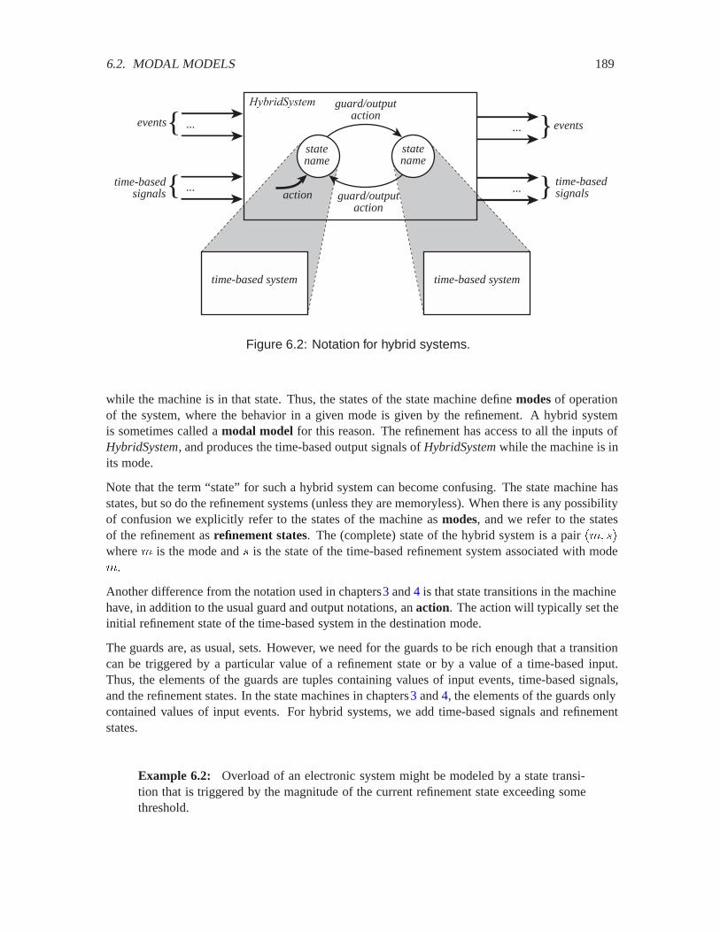
6.2. MODAL MODELS 189
guard/outputaction
guard/outputaction
statename
statename
...{events
...{time-basedsignals
... }events
... } time-basedsignals
time-based system time-based system
action
HybridSystem
Figure 6.2: Notation for hybrid systems.
while the machine is in that state. Thus, the states of the state machine define modes of operationof the system, where the behavior in a given mode is given by the refinement. A hybrid systemis sometimes called a modal model for this reason. The refinement has access to all the inputs ofHybridSystem, and produces the time-based output signals of HybridSystemwhile the machine is inits mode.
Note that the term “state” for such a hybrid system can become confusing. The state machine hasstates, but so do the refinement systems (unless they are memoryless). When there is any possibilityof confusion we explicitly refer to the states of the machine as modes, and we refer to the statesof the refinement as refinement states. The (complete) state of the hybrid system is a pair �'� ��where ' is the mode and � is the state of the time-based refinement system associated with mode'.
Another difference from the notation used in chapters3 and 4 is that state transitions in the machinehave, in addition to the usual guard and output notations, an action. The action will typically set theinitial refinement state of the time-based system in the destination mode.
The guards are, as usual, sets. However, we need for the guards to be rich enough that a transitioncan be triggered by a particular value of a refinement state or by a value of a time-based input.Thus, the elements of the guards are tuples containing values of input events, time-based signals,and the refinement states. In the state machines in chapters3 and 4, the elements of the guards onlycontained values of input events. For hybrid systems, we add time-based signals and refinementstates.
Example 6.2: Overload of an electronic system might be modeled by a state transi-tion that is triggered by the magnitude of the current refinement state exceeding somethreshold.
190 CHAPTER 6. HYBRID SYSTEMS
On the other hand, when the system is in some mode, the refinement state is only affected by thetime-based inputs. It is not affected by the event inputs. This keeps the time-based models simple,so that they don’t have to deal with stuttering inputs.
Correspondingly, the time-based outputs are generated by the refinement, and hence need not bementioned after the slash on the transitions.
The state machine may react at any time in the time base . The mode in which it is beforethis reaction is called the current mode. It will take a discrete state transition and switch to thedestination mode if the input values and the refinement state at that time match a guard. If it doesnot take a discrete state transition, then the state machine stutters. In either case, the refinement ofthe current mode also reacts to the time-based inputs, changes its state and produces outputs.
Example 6.3: Many high-end audio systems offer “digital signal processing.” Such asystem typically has an embedded computer (a digital signal processor or DSP, see boxon page 320). This computer is used to process the audio signal in various ways, forexample to add reverberation or to perform frequency selective filtering. A particularlysimple function that might be performed is loudness compensation, something offeredby all but the cheapest audio systems.
At low volumes, the human ear is less sensitive to low frequencies (base notes) thanto high frequencies. Loudness compensation boosts the low frequencies. This is donesimply by implementing a filter, which is a linear time-invariant system that can bedescribed by a state-space model, as in the previous chapter. Thus, there are two modes,one where the low frequencies are boosted (using the filter), and one where they are not.
A simple realization of loudness compensation offers a switch on a control panel toturn on and off the compensation. Figure 6.3 shows a hybrid system that reacts to inputevents from this switch to select from among two modes. The upper input is simply anevent indicating the position of the control switch when it is thrown. The lower input �is a discrete-time signal, probably sampled at 44,100 samples/second, the CD rate. TheLoudnessCompensationhybrid system has two modes. In the flat mode, the output � issimply set equal to the input �. That is, if $ �� � Integersis the time indexes duringwhich the machine is in the flat mode, then
� � $ ��� ���� � �����
This (obviously) does not boost low frequencies, since the output is equal to the input.
When the on event occurs, the machine transitions to the boostmode, where the filteris applied to the input �. This is done using the state update and output equations
� � �""��� ���� � � ����� � �����
���� � !� ���� � ������
where �� �� !� � are chosen to boost the low frequencies (how to do that is explained inchapter 9).
Note that in the flat mode, even though the output equation does not depend on the state,the state update equation is still applied. This ensures that when switching between
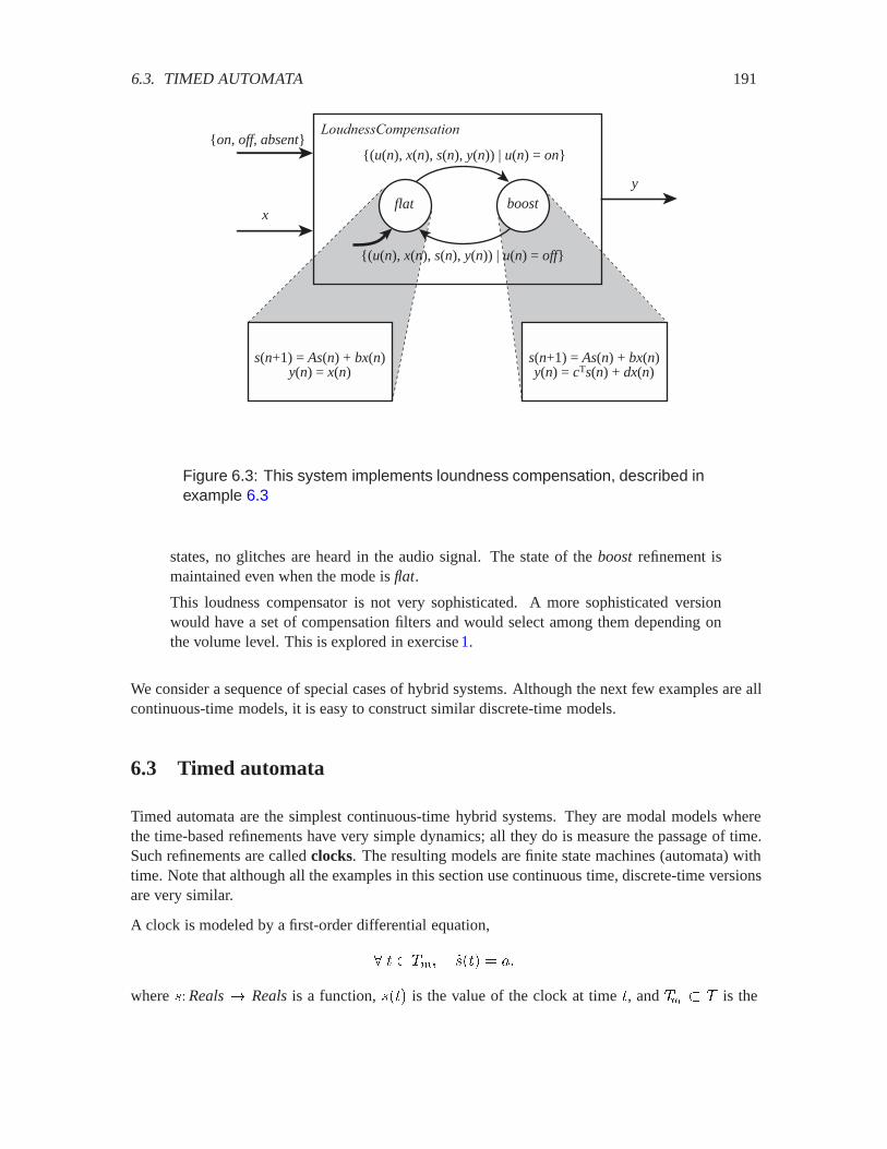
6.3. TIMED AUTOMATA 191
{(u(n), x(n), s(n), y(n)) | u(n) = on}
flat boost
s(n+1) = As(n) + bx(n)y(n) = x(n)
LoudnessCompensation
x
y
{on, off, absent}
{(u(n), x(n), s(n), y(n)) | u(n) = off}
s(n+1) = As(n) + bx(n)y(n) = cTs(n) + dx(n)
Figure 6.3: This system implements loundness compensation, described inexample 6.3
states, no glitches are heard in the audio signal. The state of the boostrefinement ismaintained even when the mode is flat.
This loudness compensator is not very sophisticated. A more sophisticated versionwould have a set of compensation filters and would select among them depending onthe volume level. This is explored in exercise 1.
We consider a sequence of special cases of hybrid systems. Although the next few examples are allcontinuous-time models, it is easy to construct similar discrete-time models.
6.3 Timed automata
Timed automata are the simplest continuous-time hybrid systems. They are modal models wherethe time-based refinements have very simple dynamics; all they do is measure the passage of time.Such refinements are called clocks. The resulting models are finite state machines (automata) withtime. Note that although all the examples in this section use continuous time, discrete-time versionsare very similar.
A clock is modeled by a first-order differential equation,
� �� ���� � ��
where ��Reals� Realsis a function, ��� is the value of the clock at time , and � � is the

192 CHAPTER 6. HYBRID SYSTEMS
{s(t) | s(t) = 1} / ticks(t) := 0
mode 1 mode 2
s(t) = 1
tickGenerator
{s(t) | s(t) = 2} / ticks(t) := 0
.s(t) = 1.
v(t) ∈{tick, absent}
s(t) ∈ Reals
s(0) := 0
Figure 6.4: This hybrid system generates tick at time intervals alternatingbetween 1 and 2 seconds. It is a timed automaton.
subset of time during which the hybrid system is in mode '. The rate of the clock, �, is a constantwhile the system is in this mode.
Example 6.4: Suppose we want to produce a sequence of output events called tickwith the time between two consecutive ticks alternating between 1 and 2 seconds. Thatis, we want to produce a tick at times � �� �� � �� �� .A hybrid system tickGeneratorthat does this is illustrated in figure6.4. There are twomodes labeled mode 1and mode 2. The refinement state in each mode is the value ofa clock at time , denoted by � Reals. So at any time the state of tickGeneratoristhe pair �mode��� ����. The output is the event signal " and the time-based signal �.There is no input.
In both modes, � evolves according to the differential equation ���� � , where ����is the derivative of � with respect to time evaluated at some time . Thus, � simplymeasures the passage of time, with its value rising 1 second for every second of elapsedtime.
The behavior of the system is shown in figure 6.5. At time 0, as indicated by the boldarrow in figure 6.4, the system initially enters mode 1. The bold arrow has an action,“��� �� ,” which sets ��� to 0. The notation “:=” is used instead of “=” to emphasizethat this is an assignment, not an assertion (see sectionA.1.1).
In this example, there is no input, so a guard is a subset of the possible values (Reals)of the refinement states. The guard on the transition from mode 1to mode 2is
���� � ��� � �

6.3. TIMED AUTOMATA 193
mode(t)
t...(a)
(b)
(c)
s(t)
t...
v(t)
t...absenttick
0 1 3 4
Figure 6.5: (a) The modes of the hybrid system of figure 6.4, (b) the refine-ment state �, and (c) the discrete event output ".
which is satisfied one time unit after beginning. For all �� �, ��� � . At time � , this guard is satisfied, the transition is taken, and the output event "�� � tick isproduced. For all �� �, "�� has value absent.
This transition also has an action, “��� �� ,” which resets � to zero. This gives theinitial condition for the refinement system of the destination mode. In our definition,at time � , ��� � , even though the action seems to contradict this. This isemphasized in figure 6.5 by showing with a bold dot the value of � at each discontinuity.The action ��� �� is merely providing the initial conditions for the refinement of thedestination mode. But the destination mode is not active until 2 , so the action issetting ���� to 0, where � denotes a time infinitesimally larger than 1.
For �� ��, the system remains in mode 2, evolving according to the differentialequation
���� � �
��� � �
So for ) � �,
��� � ��� �
� �
�� � � �
At time � �, the guard on the arc from mode 2to mode 1is satisfied, so the transitionis taken. The output event tick is again produced, and � is reset to 0 again.
Notice in figure 6.5 that the output " is absentfor all but a few discrete values of Reals. Thissignal is called a discrete event signal for this reason. Of course, this signal can also be reinterpreted

194 CHAPTER 6. HYBRID SYSTEMS
nickel / absents(t) := 5
expired safe
s(t) = 0
parkingMeter
timeout / expired
.s(t) = −1.
v(t) ∈{expired, absent}
s(0) := 0
u(t) ∈{coin5, coin25, absent}
quarter / absents(t) := 25
nickel / absents(t) := min(s(t) + 5, 60)
quarter / absents(t) := min(s(t) + 25, 60)
timeout = {(u(t), s(t)) | u(t) = absent and s(t) = 0}nickel = {(u(t), s(t)) | u(t) = coin5}
quarter = {(u(t), s(t)) | u(t) = coin25}
Figure 6.6: A hybrid system representation of a 60-minute parking meter.
as a sequence of tick events with an arbitrary number of stuttering events in between. That signalcould therefore be supplied as input to an ordinary state machine, enabling compositions of ordinarystate machines with hybrid systems.
Also notice in figure 6.5 that the hybrid system evolves in alternating phases: there is a time-passage phase in which the system stays in the same mode and its refinement state changes withthe passage of time; this is followed by an instantaneous discrete-event phase in which a modetransition occurs, an output event is produced, and the refinement state in the destination mode isinitialized. In the figure, the time-passage phases are �� �� �� ��� ��� ��� and the discrete-eventphases occur at � �� �� .Transitions between modes have actions associated with them. Sometimes, it is useful to havetransitions from one mode back to itself, just so that the action can be realized. This is illustrated inthe next example.
Example 6.5: Figure 6.6 shows a hybrid system representation of the 60-minute park-ing meter considered in chapter 3. In the version in figure 3.6, the states of a statemachine are used to measure the passage of time by counting ticks provided by the en-vironment. In the hybrid version of figure6.6, the passage of time is explicitly modeledby first-order differential equations.
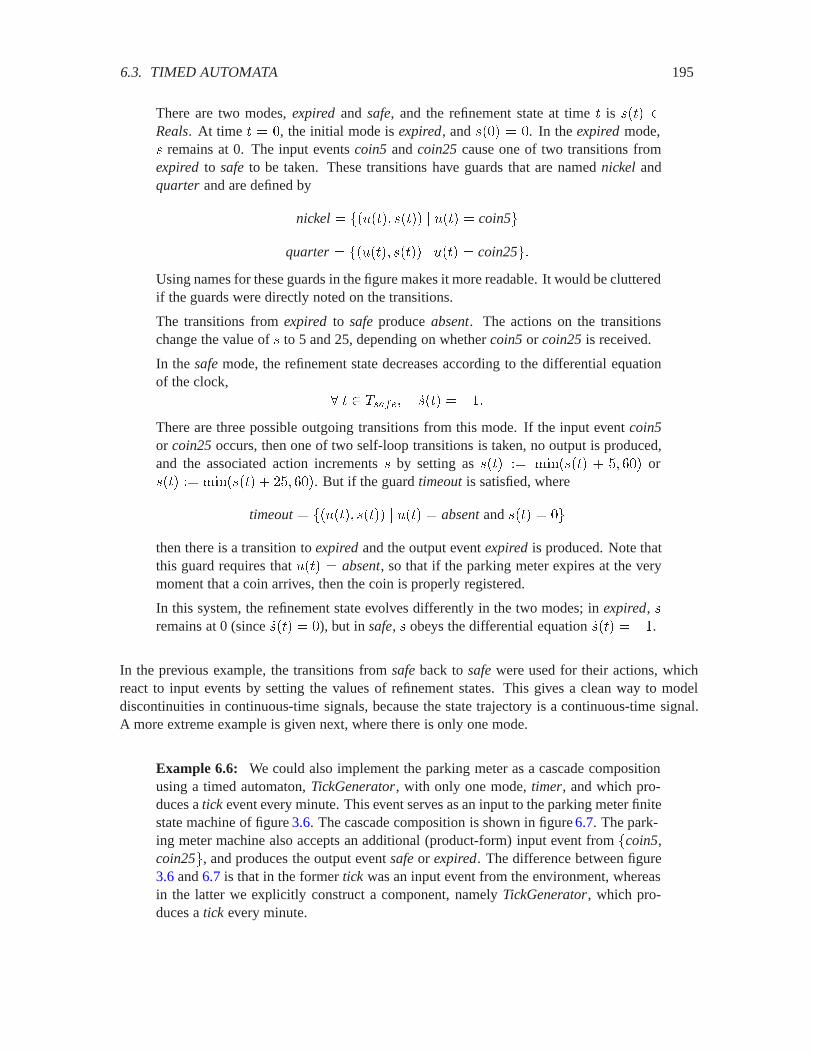
6.3. TIMED AUTOMATA 195
There are two modes, expiredand safe, and the refinement state at time is ��� Reals. At time � , the initial mode is expired, and ��� � . In the expiredmode,� remains at 0. The input events coin5 and coin25cause one of two transitions fromexpired to safeto be taken. These transitions have guards that are named nickel andquarter and are defined by
nickel� ��0��� ���� � 0�� � coin5
quarter� ��0��� ���� � 0�� � coin25�Using names for these guards in the figure makes it more readable. It would be clutteredif the guards were directly noted on the transitions.
The transitions from expired to safeproduce absent. The actions on the transitionschange the value of � to 5 and 25, depending on whether coin5or coin25is received.
In the safemode, the refinement state decreases according to the differential equationof the clock,
� ��$ � ���� � ��There are three possible outgoing transitions from this mode. If the input event coin5or coin25occurs, then one of two self-loop transitions is taken, no output is produced,and the associated action increments � by setting as ��� �� ������� � �� � or��� �� ������� � ��� �. But if the guard timeoutis satisfied, where
timeout� ��0��� ���� � 0�� � absentand ��� �
then there is a transition to expiredand the output event expiredis produced. Note thatthis guard requires that 0�� � absent, so that if the parking meter expires at the verymoment that a coin arrives, then the coin is properly registered.
In this system, the refinement state evolves differently in the two modes; in expired, �remains at 0 (since ���� � ), but in safe, � obeys the differential equation ���� � �.
In the previous example, the transitions from safeback to safewere used for their actions, whichreact to input events by setting the values of refinement states. This gives a clean way to modeldiscontinuities in continuous-time signals, because the state trajectory is a continuous-time signal.A more extreme example is given next, where there is only one mode.
Example 6.6: We could also implement the parking meter as a cascade compositionusing a timed automaton, TickGenerator, with only one mode, timer, and which pro-duces a tick event every minute. This event serves as an input to the parking meter finitestate machine of figure 3.6. The cascade composition is shown in figure 6.7. The park-ing meter machine also accepts an additional (product-form) input event from �coin5,coin25, and produces the output event safeor expired. The difference between figure3.6 and 6.7 is that in the former tick was an input event from the environment, whereasin the latter we explicitly construct a component, namely TickGenerator, which pro-duces a tick every minute.

196 CHAPTER 6. HYBRID SYSTEMS
timer
s(t) = 1
TickGenerator
.
v(t) ∈{safe,expired, absent}
s(0) := 0
{s(t) | s(t) = 1} / ticks(t) := 0 v(t) ∈{tick,
absent}parkingmeterstate
machine
u(t) ∈{coin5, coin25, absent}
Figure 6.7: The 60-minute parking meter as a cascade composition oftickGenerator and an ordinary finite state machine.
Timed automata are commonly used in modeling communication protocols, the logic used toachieve communication over a network. The following example models the transport layer of asender of data on the internet.
Example 6.7: Consider how an application such as an e-mail program sends a fileover a communication network like the internet. There are two host computers calledthe Senderand Receiver. The file that Senderwants to send to Receiveris first dividedinto a sequence of finite bit strings called packets. For the purposes of this example,we do not care what is contained by the packets, so we consider packetto be an event.We are interested in the fact that it needs to be transmitted, not in its contents.
The problem we address in this example is that the network is unreliable. Packetsthat are launched into it may never emerge. If the network is congested, packets getdropped. We will design a protocol whereby the sender of a packet waits a certainamount of time for an acknowledgement. If it does not receive the acknowledgement inthat time, then it retransmits the packet. This is an ideal application for timed automata.
The upper diagram in figure 6.8 shows the structure of the communication system. Ev-erything begins when the sender produces a packetevent. The SenderProtocolsystemreacts by producing a transmit event, which instructs its network interface card orNIC to launch the packet into the internet. The NIC is the physical device (such asthe ethernet card in your desktop computer) that converts the packet into the appropri-ate electrical signal that is transmitted through the network. The internet transfers this
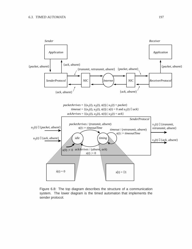
6.3. TIMED AUTOMATA 197
Application
Sender
SenderProtocol
{packet, absent}{ack, absent}
NIC Internet NIC ReceiverProtocol
Application
Receiver
{packet, absent}
{ack, absent}
{transmit, retransmit, absent} {packet, absent}
{ack, absent}
packetArrives / (transmit, absent)s(t) := timeoutTime
idle timing
s(t) = 0
SenderProtocol
ackArrives / (absent, ack)s(t) := 0
.s(t) = −1.
v1(t) ∈{transmit, retransmit, absent}
s(0) := 0
v2(t) ∈{ack, absent}
timeout / (retransmit, absent)s(t) := timeoutTime
u1(t) ∈{packet, absent}
u2(t) ∈{ack, absent}
timeout = {(u1(t), u2(t), s(t)) | s(t) = 0 and u1(t) ≠ ack}packetArrives = {(u1(t), u2(t), s(t)) | u1(t) = packet}
ackArrives = {(u1(t), u2(t), s(t)) | u2(t) = ack}
Figure 6.8: The top diagram describes the structure of a communicationsystem. The lower diagram is the timed automaton that implements thesender protocol.

198 CHAPTER 6. HYBRID SYSTEMS
signal to the NIC of the receiver. That NIC converts the signal back into the packetand forwards it to the ReceiverProtocolcomponent. The ReceiverProtocolin turn for-wards the packet to the e-mail application in the Receiverand simultaneously sends anacknowledgement packet, called ack, to its NIC.
The receiver’s NIC sends the ack packet back through the network to the Sender. Thesender’s NIC receives this packet and forwards an ack to the SenderProtocol. TheSenderProtocolnotifies the application that the packet was indeed delivered. The ap-plication can now send the next packet, and the cycle is repeated until the entire file isdelivered.
In reality, the network may drop the packet so that it is not delivered to the receiver, whotherefore will not send the corresponding ack. The SenderProtocolsystem is designedto take care of this contingency. It is a timed automaton with two modes, idle andtiming, and one refinement state � corresponding to a clock. Initially it is in the idlemode and ��� � . In the idle mode, ���� � , so the refinement state remains at zero.When SenderProtocolreceives a packetit makes a transition to the timing mode, sendsthe output event transmitto its NIC, and resets � to a timeout value timeoutTime.
In the timing mode, there are two possibile transitions. In the normal case, the inputevent ack is received before the guard ���� �� is satisfied. The transition to modeidle is taken, the output event ack is sent to the application, and the clock value ���is reset to 0. The system waits for another packetfrom the application. In the secondcase, the guard ���� �� is satisfied (before event ack), and the self-loop transitionis taken. In this case, the output event retransmitis sent to the NIC, and ��� is reset totimeoutTime.
Notice a feature of this design that may not be expected. If a packet arrives while themachine is in mode timing, the packet is ignored. What happens if a packet happens toarrive simultaneously with an ackwhile the machine is mode timing?
Exercise 10 asks you to construct the corresponding receiver protocol, which is simpler.
In summary, the SenderProtocolmachine repeatedly retransmits a packet every timeoutTimeseconds until it receives an ack. This reveals a flaw in the protocol. If the network is forsome reason unable ever to successfully transmit a packet to the receiver, the machinewill continue retransmission for ever. A better protocol would retransmit a packet acertain number of times, say five times, and if it is unsuccessful, it would return to idleand send a message connectionFailedto the application. The hybrid system of figure6.9 incorporates this feature by adding another clock whose value is ���.
6.4 More interesting dynamics
In timed automata, all that happens in the time-based refinement systems is that time passes. Hybridsystems, however, are much more interesting when the behavior of the refinements is more complex.
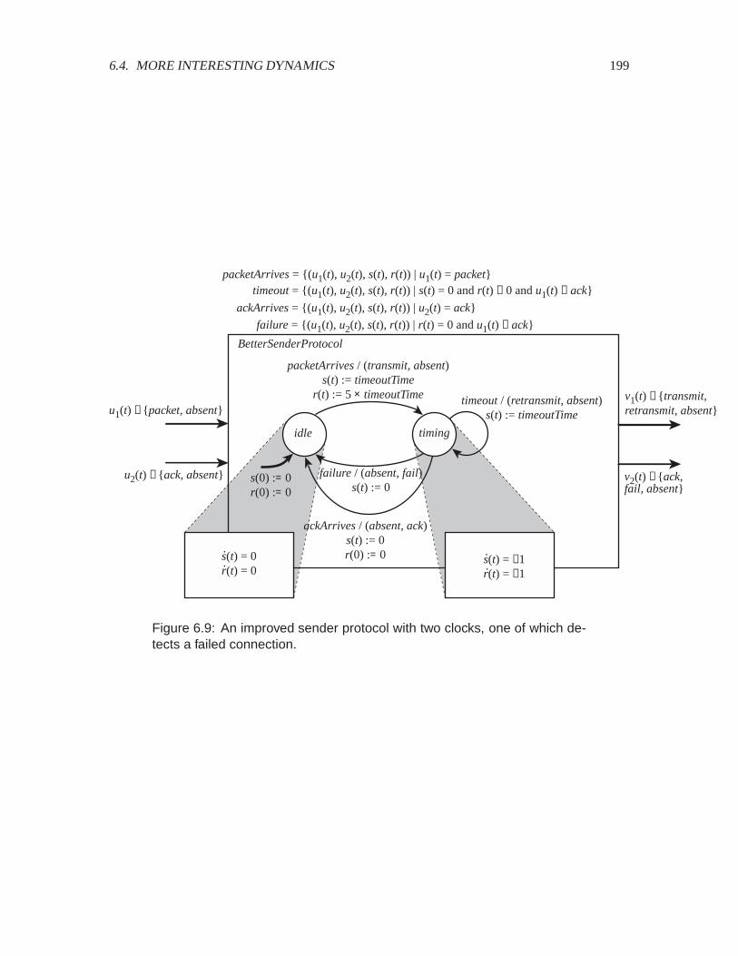
6.4. MORE INTERESTING DYNAMICS 199
packetArrives / (transmit, absent)s(t) := timeoutTime
r(t) := 5 × timeoutTime
idle timing
s(t) = 0r(t) = 0
BetterSenderProtocol
ackArrives / (absent, ack)s(t) := 0r(0) := 0.
s(t) = −1r(t) = −1
.
s(0) := 0r(0) := 0
timeout / (retransmit, absent)s(t) := timeoutTime
. .
failure / (absent, fail)s(t) := 0
timeout = {(u1(t), u2(t), s(t), r(t)) | s(t) = 0 and r(t) ≠ 0 and u1(t) ≠ ack}packetArrives = {(u1(t), u2(t), s(t), r(t)) | u1(t) = packet}
ackArrives = {(u1(t), u2(t), s(t), r(t)) | u2(t) = ack}
v1(t) ∈{transmit, retransmit, absent}
v2(t) ∈{ack,fail, absent}
u1(t) ∈{packet, absent}
u2(t) ∈{ack, absent}
failure = {(u1(t), u2(t), s(t), r(t)) | r(t) = 0 and u1(t) ≠ ack}
Figure 6.9: An improved sender protocol with two clocks, one of which de-tects a failed connection.

200 CHAPTER 6. HYBRID SYSTEMS
Probing further: Internet protocols
Communication between two computers, Senderand Receiver, each connected tothe internet, is coordinated by a set of protocols. Each protocol can be modeled bya pair of hybrid systems, one in the Senderand the other in the Receiver. Theseprotocols are arranged in a protocol stack, as shown in figure6.10. Each layer inthe stack performs a certain function, and interacts with the corresponding layer inthe other computer. The physical layer converts a bit stream into an electrical signaland vice versa and transfers the signal over one link of the network.
The network itself consists of many physical links connected by routers. Therouters themselves act as computers, but are missing the higher levels of the pro-tocol stack. The physical layer transports bits over wires, optical fibers, or radiolinks. The medium access layer manages contention for the physical communica-tion resource, preventing collisions among multiple users of the link. The networklayer routes packets appropriately through the network. The transport layer en-sures that the end-to-end transfer of packets is reliable, even if the network layerservice is unreliable. The application layer converts whatever information is tobe sent (such as an image or e-mail) into packets and then reassembles the packetsinto the appropriate information.
This layered approach provides an abstractionmechanism. Each layer conceptu-ally interacts with the corresponding layer at a remote machine, as suggested bythe dotted lines in figure 6.10. Each layer provides a “service” to the layer above it,using the service offered by the layer underneath. For example, the medium accesslayer offers as a service the transfer of a packet over a single link. The networklayer uses this service to transfer a packet over a sequence of links between theend hosts. This abstraction mechanism permits the design of a single layer, saythe transport layer, assuming the service of the network layer, without regard to thelayers below the network layer. The hybrid system in example 6.7, for instance,models only the transport layer.
The transport layer in an end-to-end protocol, so it is implemented only at the endpoints in the connection, as shown in figure 6.10. The routers in the network onlyneed to implement the lower layers.
As mentioned, each protocol layer is modeled as a pair of hybrid systems. Typi-cally, these are timed automata, since coordination between end hosts is achievedvia several clocks as in example 6.7. When a guard associated with a clock is sat-isfied, this signals some contingency in the communication, just as the timeout ofthe clock in figure 6.8 signals that a packet may be lost.
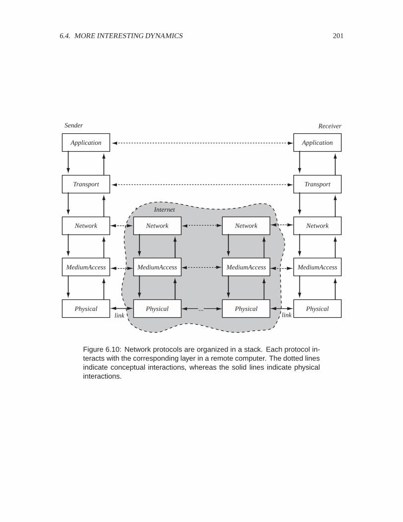
6.4. MORE INTERESTING DYNAMICS 201
Application
Transport
Network
MediumAccess
Physical
Network
MediumAccess
Physical
Network
MediumAccess
Physical
Application
Transport
Network
MediumAccess
Physical...
Internet
link link
Sender Receiver
Figure 6.10: Network protocols are organized in a stack. Each protocol in-teracts with the corresponding layer in a remote computer. The dotted linesindicate conceptual interactions, whereas the solid lines indicate physicalinteractions.
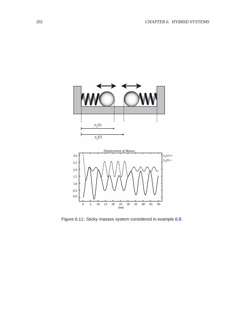
202 CHAPTER 6. HYBRID SYSTEMS
y1(t)
y2(t)
y1(t)
y2(t)
0.0
0.5
1.0
1.5
2.0
2.5
3.0
0 5 10 15 20 25 30 35 40 45 50
Displacement of Masses
time
Figure 6.11: Sticky masses system considered in example 6.8.

6.4. MORE INTERESTING DYNAMICS 203
Example 6.8: Consider the physical system depicted in figure6.11. Two sticky roundmasses are attached to springs. The springs are compressed or extended and then re-leased. The masses oscillate on a frictionless table. If they collide, they stick togetherand oscillate together. After some time, the stickiness decays, and masses pull apartagain.
A plot of the displacement of the two masses as a function of time is shown in the figure.Both springs begin compressed, so the masses begin moving towards one another. Theyalmost immediately collide, and then oscillate together for a brief period until they pullapart. In this plot, they collide two more times, and almost collide a third time.
The physics of this problem is quite simple if we assume idealized springs. Let ����denote the right edge of the left mass at time , and ���� denote the left edge of theright mass at time , as shown in figure 6.11. Let (� and (� denote the neutral positionsof the two masses, i.e. when the springs are neither extended nor compressed, so theforce is zero. For an ideal spring, the force at time on the mass is proportional to(� � ���� (for the left mass) and (� � ���� (for the right mass). The force is positiveto the right and negative to the left.
Let the spring constants be 6� and 6�, respectively. Then the force on the left spring is6��(� � �����, and the force on the left spring is 6��(� � �����. Let the masses be'� and '� respectively. Now we can use Newton’s law, which relates force, mass, andacceleration,
� � '��
The acceleration is the second derivative of the position with respect to time, whichwe write ����� and ����� respectively. Thus, as long as the masses are separate, theirdynamics are given by
����� � 6��(� � ������'� (6.1)
����� � 6��(� � ������'�� (6.2)
When the masses collide, however, the situation changes. With the masses stuck to-gether, they behave as a single object with mass '��'�. This single object is pulled inopposite directions by two springs. While the masses are stuck together, ���� � ����.Let
��� � ���� � �����
The dynamics are then given by
���� �6�(� � 6�(� � �6� � 6�����
'� �'�� (6.3)
It is easy to see now how to construct a hybrid systems model for this physical system.The model is shown in figure 6.12. It has two modes, apart and together. The refine-ment of the apart mode is given by (6.1) and (6.2), while the refinement of the togethermode is given by (6.3).
We still have work to do, however, to label the transitions. The initial transition is shownin figure 6.12 entering the apart mode. Thus, we are assuming the masses begin apart.
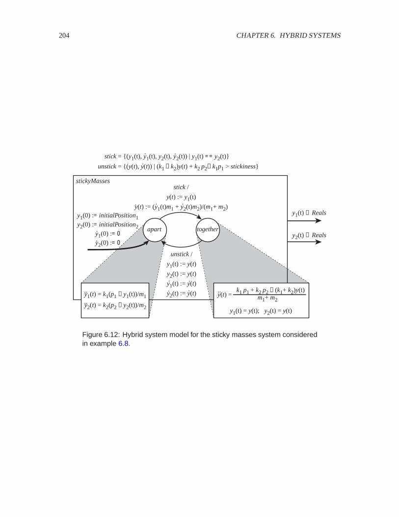
204 CHAPTER 6. HYBRID SYSTEMS
stick /
y(t) := y1(t)
y(t) := (y1(t)m1 + y2(t)m2)/(m1+ m2)
apart together
y1(t) = k1(p1 − y1(t))/m1
stickyMasses
unstick /
y1(t) := y(t)
y2(t) := y(t)
y1(t) := y(t)
y2(t) := y(t)..
y1(t) ∈ Reals
y2(t) ∈ Reals
y1(0) := initialPosition1y2(0) := initialPosition2
y1(0) := 0y2(0) := 0
y2(t) = k2(p2 − y2(t))/m2..
y(t) =.. k1 p1 + k2 p2 − (k1+ k2)y(t)
m1+ m2
.
.
.
.
.
.
.
. .
y1(t) = y(t); y2(t) = y(t)
unstick = {(y(t), y(t)) | (k1 − k2)y(t) + k2 p2− k1p1 > stickiness}.
stick = {(y1(t), y1(t), y2(t), y2(t)) | y1(t) = = y2(t)}. .
Figure 6.12: Hybrid system model for the sticky masses system consideredin example 6.8.

6.4. MORE INTERESTING DYNAMICS 205
Moreover, this transition is labeled with an action that sets the initial refinement state.Intuitively, the initial state of the masses is their positions and their initial velocities. Infact, we can define the refinement state to be
��� �
�����������������������
����� �
It is then a simple matter to rewrite (6.1) and (6.2) in the form
���� � ������ (6.4)
for a suitably chosen function � (see exercise12).
In figure 6.12, the initial state has the masses at some specified displacement, and thevelocities at zero.
The transition from apart to togetherhas the guard
stick� ������� ������ ����� ������ � ���� �� �����Thus, when the refinement state of apart satisfies this guard, the transition will betaken. No event output is produced, as indicated by the blank after the slash. However,an action is taken to set the initial refinement state of together. The refinement state oftogethercould be the same ��� as above, with the additional constraint that ���� ����� and ����� � �����, because the masses are stuck together. Or more simply, wecould define the state ��� of togetherto be the position ��� and velocity ����, where��� � ���� � ����,
��� �
�������
��
The transition from apart to togethersets ��� equal to ���� (it could equally well havechosen ����, since these are equal). It sets the velocity to conserve momentum. Themomentum of the left mass is �����'�, the momentum of the right mass is �����'�,and the momentum of the combined masses is �����'� �'��. To make these equal, itsets
���� ������'� � �����'�
'� �'��
The transition from togetherto apart has the more complicated guard
unstick� ������ ����� � �6� � 6����� � 6�(� � 6�(� 2 stickiness�This guard is satisfied when the right-pulling force on the right mass exceeds the right-pulling force on the left mass by more than the stickiness. The right-pulling force onthe right mass is simply
���� � 6��(� � ����
and the right-pulling force on the left mass is
���� � 6��(� � �����
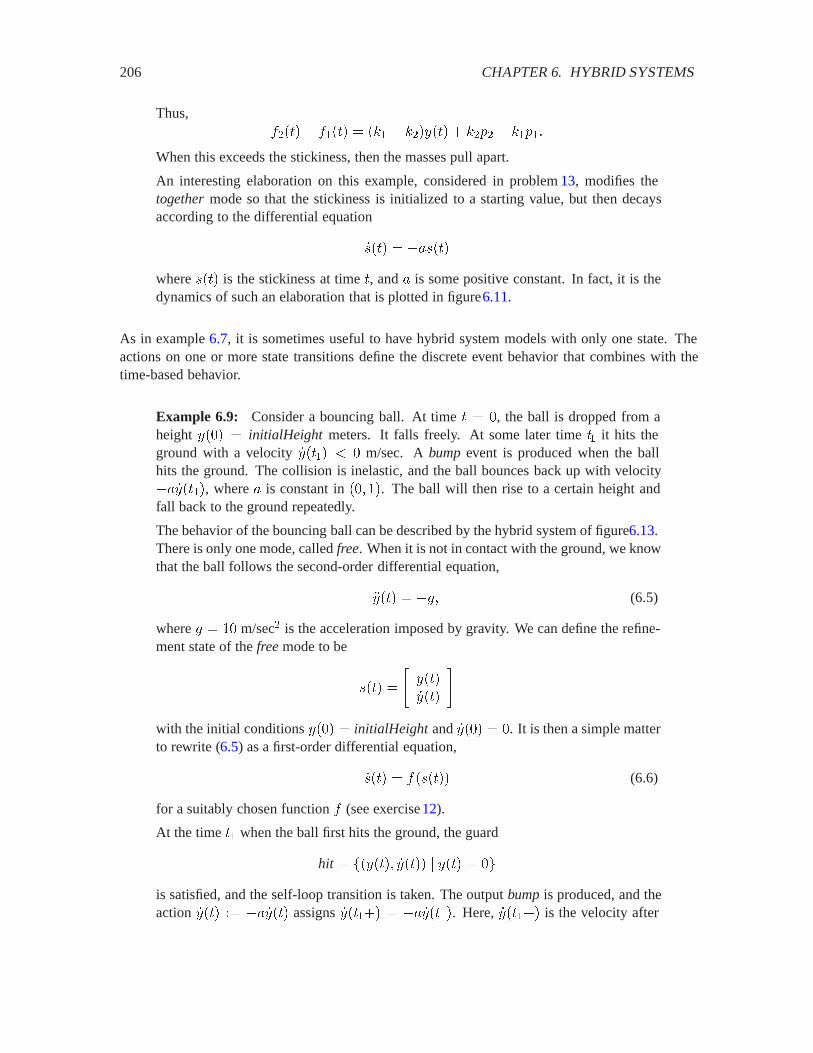
206 CHAPTER 6. HYBRID SYSTEMS
Thus,����� ���� � �6� � 6����� � 6�(� � 6�(��
When this exceeds the stickiness, then the masses pull apart.
An interesting elaboration on this example, considered in problem 13, modifies thetogethermode so that the stickiness is initialized to a starting value, but then decaysaccording to the differential equation
���� � �����where ��� is the stickiness at time , and � is some positive constant. In fact, it is thedynamics of such an elaboration that is plotted in figure6.11.
As in example 6.7, it is sometimes useful to have hybrid system models with only one state. Theactions on one or more state transitions define the discrete event behavior that combines with thetime-based behavior.
Example 6.9: Consider a bouncing ball. At time � , the ball is dropped from aheight ��� � initialHeight meters. It falls freely. At some later time � it hits theground with a velocity ����� ) m/sec. A bumpevent is produced when the ballhits the ground. The collision is inelastic, and the ball bounces back up with velocity�� �����, where � is constant in �� �. The ball will then rise to a certain height andfall back to the ground repeatedly.
The behavior of the bouncing ball can be described by the hybrid system of figure6.13.There is only one mode, called free. When it is not in contact with the ground, we knowthat the ball follows the second-order differential equation,
���� � ��� (6.5)
where � � m/sec� is the acceleration imposed by gravity. We can define the refine-ment state of the freemode to be
��� �
�������
�
with the initial conditions ��� � initialHeight and ���� � . It is then a simple matterto rewrite (6.5) as a first-order differential equation,
���� � ������ (6.6)
for a suitably chosen function � (see exercise12).
At the time � when the ball first hits the ground, the guard
hit � ������ ����� � ��� � is satisfied, and the self-loop transition is taken. The output bumpis produced, and theaction ���� �� �� ���� assigns ������ � �� �����. Here, ������ is the velocity after
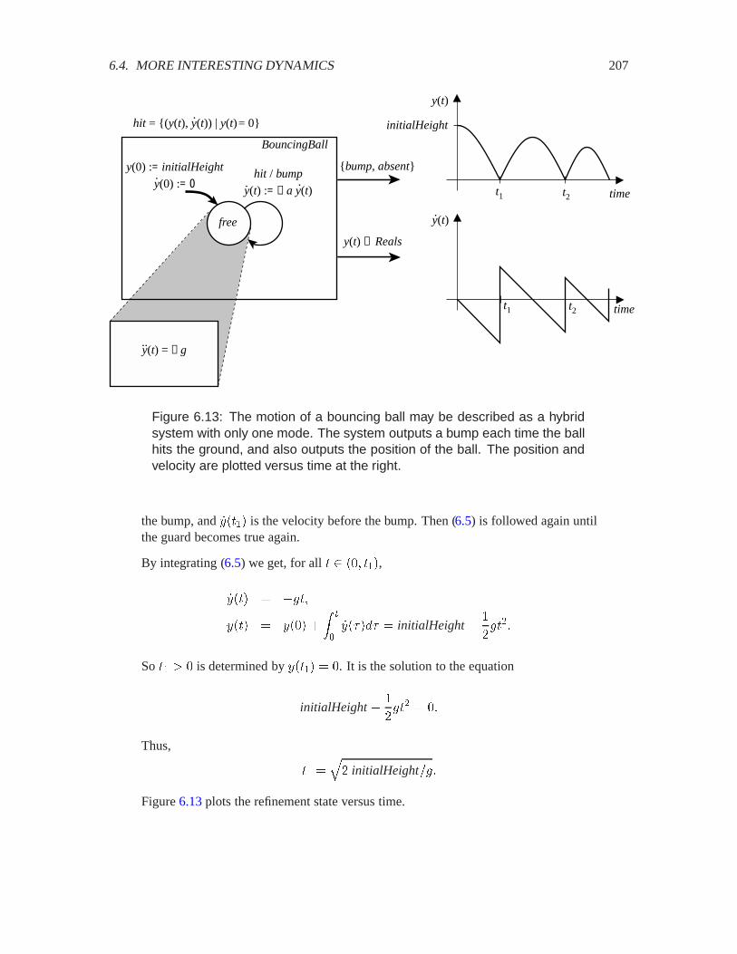
6.4. MORE INTERESTING DYNAMICS 207
free
y(t) = − g
BouncingBall
..
y(0) := initialHeight
y(0) := 0hit / bump
y(t) := − a y(t)
y(t) ∈ Reals
.{bump, absent}
. .
initialHeight
y(t)
t1 t2 time
y(t)
t1 t2 time
.
hit = {(y(t), y(t)) | y(t) = 0}.
Figure 6.13: The motion of a bouncing ball may be described as a hybridsystem with only one mode. The system outputs a bump each time the ballhits the ground, and also outputs the position of the ball. The position andvelocity are plotted versus time at the right.
the bump, and ����� is the velocity before the bump. Then (6.5) is followed again untilthe guard becomes true again.
By integrating (6.5) we get, for all �� ��,
���� � ������ � ��� �
� �
�������� � initialHeight�
����
So � 2 is determined by ���� � . It is the solution to the equation
initialHeight�
��� � �
Thus,
� ��� initialHeight���
Figure 6.13 plots the refinement state versus time.
208 CHAPTER 6. HYBRID SYSTEMS
6.5 Supervisory control
We introduce supervisory control through a detailed example. A control system involves four com-ponents. There is a system called the plant—the physical process that is to be controlled; theenvironment in which the plant operates; the sensors that measure some variables of the plant andthe environment; and the controller that determines the mode transition structure and selects thetime-based inputs to the plant. The controller has two levels: the supervisory control that deter-mines the mode transition structure, and the ‘low-level’ control that selects the time-based inputswhich control the behavior of the refinements. A complete design includes both levels of control asin the following example.
Example 6.10: The plant is an automated guided vehicle or AGV that moves alonga closed track painted on a warehouse or factory floor. We will design a controller sothat the vehicle closely follows the track.
The vehicle has two degrees of freedom. At any time , it can move forward along itsbody axis with speed 0�� with the restriction that � 0�� � mph. It can also rotateabout its center of gravity with an angular speed ��� restricted to �� � ��� � �radians/second. We ignore the inertia of the vehicle.
Let ����� ���� Reals� be the position and <�� ���� �� the angle (in radians) ofthe vehicle at time relative to some fixed coordinate frame, as shown on the left infigure 6.14. In terms of this coordinate frame, the motion of the vehicle is given by asystem of three differential equations,
���� � 0�� ��� <���
���� � 0�� ���<��� (6.7)�<�� � ����
The track and the vehicle are shown on the right of figure6.14. Equations (6.7) describethe plant. The environment is the closed painted track. It could be described by anequation. We will describe it indirectly below by means of a sensor.
The two-level controller design is based on a simple idea. The vehicle always movesat its maximum speed of 10 mph. If the vehicle strays too far to the left of the track,the controller steers it towards the right; if it strays too far to the right of the track, thecontroller steers it towards the left. If the vehicle is close to the track, the controllermaintains the vehicle in a straight direction. Thus the controller guides the vehicle infour modes, left, right, straight, and stop. In stop mode an operator may bring thevehicle to a halt.
The following differential equations govern the AGV’s motion in the refinement of thefour modes. They describe the low-level controller, i.e. the selection of the time-basedinputs in each mode.
straight
���� � ��� <��

6.5. SUPERVISORY CONTROL 209
x(t)
y(t)AGV
globalcoordinate
frame
e(t)
track
(t)
Figure 6.14: Illustration of the automated guided vehicle of example 6.10.The vehicle is shown as a large arrow on the left and as a small arrow on theright. On the right, the vehicle is following a curved painted track, and hasdeviated from the track by a distance ���. The coordinates of the vehicle attime with respect to the global coordinate frame are ����� ���� <���.
���� � ���<��
�<�� �
left
���� � ��� <��
���� � ���<��
�<�� � �
right
���� � ��� <��
���� � ���<��
�<�� � ��stop
���� �
���� �
�<�� �
In the stopmode, the vehicle is stopped, ���� ���� <�� are constant. In the left mode,<�� increases at the rate of � radians/second, so from figure6.14 we see that the vehicle
210 CHAPTER 6. HYBRID SYSTEMS
moves to the left. In the right mode, it moves to the right. In the straight mode,<�� is constant, and the vehicle moves straight ahead with a constant heading. Therefinements of the four modes are shown in the boxes of figure6.15.
We design the supervisory control governing transitions between modes in such a waythat the vehicle closely follows the track, using a sensor that determines how far thevehicle is to the left or right of the track. We can build such a sensor using photodiodes.Let’s suppose the track is painted with a light-reflecting color, whereas the floor isrelatively dark. Underneath the AGV we place an array of photodiodes as shown infigure 6.16. The array is perpendicular to the AGV body axis. As the AGV passesover the track, the diode directly above the track generates more current than the otherdiodes. By comparing the magnitudes of the currents through the different diodes, thesensor gives the displacement ��� of the center of the array (hence, the center of theAGV) from the track. We adopt the convention that ��� ) means that the AGV is tothe right of the track and ��� 2 means it is to the left. We model the sensor outputas a function � of the AGV’s position,
�� ��� � ������ �����
The function � of course depends on the environment—the track. We now specify thesupervisory controller precisely. We select two thresholds, ) A� ) A�, as shown infigure 6.16. If the magnitude of the displacement is small, ����� ) A�, we considerthat the AGV is close enough to the track, and the AGV can move straight ahead, instraight mode. If ) A� ) ��� (��� is large and positive), the AGV has strayedtoo far to the left and must be steered to the right, by switching to right mode. If 2 �A� 2 ��� (��� is large and negative), the AGV has strayed too far to the rightand must be steered to the left, by switching to left mode. This control logic is capturedin the mode transitions of figure 6.15. The input events are �stop� start�absent. Byselecting events stopand start an operator can stop or start the AGV. There is no time-based input. There is no external output. The initial mode is stop, and the initial valuesof its refinement are ���� ��� <��.
We analyze how the AGV will move. Figure 6.17 sketches one possible trajectory.Initially the vehicle is within distance A� of the track, so it moves straight. At somelater time, the vehicle goes too far to the left, the guard
goRight� ��0��� ���� ���� <��� � 0�� �� stop� A� ) ���is satisfied, and there is a mode switch to right. After some time, the vehicle is closeenough to the track, the guard
goStraight� ��0��� ���� ���� <��� � 0�� �� stop� ����� ) A�is satisfied, and there is a mode switch to straight. Some time later, the vehicle is toofar to the right, the guard
goLeft� ��0��� ���� <��� � 0�� �� stop� � A� 2 ���is satisfied, there is a mode switch to left, and so on.

6.5. SUPERVISORY CONTROL 211
stop left
Vehicle
right straight
x (t) = 10 cos φ(t)y (t) = 10 sin φ(t) φ (t) = - πe (t) = f(x(t), y(t))
u(t) ε {stop, start, absent}
x (t) = 10 cos φ (t)y (t) = 10 sin φ (t)φ = πe (t) = f(x(t), y(t))
.
.
.
x (t) = 10 cos φ (t)y (t) = 10 sin φ (t)φ (t) = 0e (t) = f(x(t), y(t))
.
.
.
x = x0y = y0 φ = φ0
goRight/
goLeft/
x (t) = 0 y (t) = 0 φ (t) = 0e (t) = f(x(t), y(t))
.
.
.
...
goStraight= {(u(t), x(t), y(t), φ (t)) | u(t) != stop, |e(t)| < ε1}
goRight/
goStraight/
goLeft = {(u(t), x(t), y(t), φ (t)) | u(t) != stop, - ε2 > − e(t)}
goStraight/
goLeft/
goStop/ goStop/
goStop/
goStart/
goStop = {(u(t), x(t), y(t), φ (t)) | u(t) = stop}goStart = {(u(t), x(t), y(t), φ (t)) | u(t) = start}
goRight ={(u(t), x(
Figure 6.15: The automatic guided vehicle of example 6.10 has four modes:stop, straight , left , right .
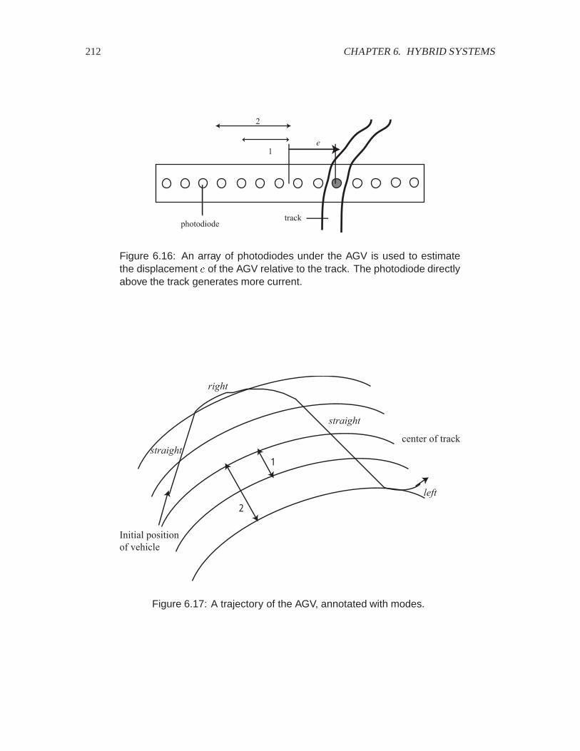
212 CHAPTER 6. HYBRID SYSTEMS
photodiodetrack
e1
2
Figure 6.16: An array of photodiodes under the AGV is used to estimatethe displacement � of the AGV relative to the track. The photodiode directlyabove the track generates more current.
center of trackstraight
right
straight
left
1
2
Initial positionof vehicle
Figure 6.17: A trajectory of the AGV, annotated with modes.
6.6. FORMAL MODEL 213
The example illustrates the four components of a control system. The plant is described by the dif-ferential equations (6.7) that govern the evolution of the refinement state at time , ����� ���� <���,in terms of the time-based input, �0��� ����. The second component is the environment—theclosed track. The third component is the sensor, whose output at time , ��� � ������ ����, givesthe position of the AGV relative to the track. The fourth component is the two-level controller.The supervisory controller comprises the four modes and the guards that determine when to switchbetween modes. The low-level controller specifies how the time-based inputs, 0 and �, are selectedin each mode.
6.6 Formal model
We develop a formal model of a hybrid system similar to the ‘sets and functions’ model of section3.1. A hybrid system HybridSystemis a 5-tuple,
HybridSystem� �States� Inputs�Outputs�TransitionStructure� initalState��
where, States, Inputs, Outputsare sets, and initalState Statesis the initial state. TransitionStructureconsists of several items that determine how the hybrid system evolves in time . may beReals� or Naturals�. Here we assume � Reals�.
States� Modes�RefinementStatesis the state space. Modesis the finite set of modes. RefinementStatesis the state space of the refinements. If the current state at time is �'��� ���� we say that the sys-tem is in mode '�� and its refinement is in state ���.
Inputs � InputEvents� TimeBasedInputsis the set of input symbols. InputEventsis the finitealphabet of discrete input symbols, including a stuttering symbol, while TimeBasedInputsis the setof input values to which the refinement reacts. An input signal consists of a pair of functions �0� ��where 0�Reals� � InputEventsand ��Reals� � TimeBasedInputs. For all except a discrete set oftimes , 0�� is the stuttering symbol, absent.
Outputs� OutputEvents� TimeBasedOutputsis the set of output symbols. OutputEventsis the fi-nite alphabet of discrete output symbols, including a stuttering output, absent, and TimeBasedOutputsis the set of continuous output values. An output signal consists of a pair of functions �"� �� where"�Reals� � OutputEventsand ��Reals� � TimeBasedOutputs. For all except a discrete set oftimes, "�� � absent.
The transition structure determines how a mode transition occurs and how the refinement statechanges over time. Suppose the inputs signal is �0� ��. Suppose at time the mode is ' and therefinement state is �. For each destination mode � there is a guard
9��% � B��% ����% � .��%
� InputEvents� TimeBasedInputs� RefinementStates�
There is also an output event, say "��%, and an action ���%�RefinmentStates� RefinmentStatesthat assigns a (possibly new) value to each refinement state, (possibly) depending on the currentvalue of the refinement state. If there is a match �0��� ���� ���� 9��%, then there is a discrete
214 CHAPTER 6. HYBRID SYSTEMS
transition at ; the mode after the transition is �, the output event "�� � "��% is produced, and therefinement state in mode � at time � immediately after the transition is set to ���� � ���%����.
If no guard is satisfied at time , then the refinement state ��� and the time-based output ��� aredetermined by the time-based input signal � according to the equations governing the refinementdynamics. Here we will need to be concrete. In all of the examples above, we have taken
RefinementStates� Reals� �
TimeBasedInputs� Reals� � and
TimeBasedOutputs� Reals� �
In this concrete setting, the refinement dynamics are given as
� �� ���� � ������� ����� (6.8)
��� � ������� ���� (6.9)
where � � is the set of times when the system is in mode ', and the functions
�� � Reals� � Reals� � � Reals� �
�� � Reals� � Reals� � � Reals�
characterize the behavior of the refinement system in mode '. The function
� � Reals� � RefinementStates
is the trajectory of the refinment states.
We can now see how the hybrid system evolves over time. At time � , the system starts in the ini-tial state, say �'��� ����. It evolves in alternating phases of time passage, �� � � ��� ��� ��� ,and discrete transitions at �� �� . During the first interval ��� ��, no guard is satisfied and thesystem remains in mode '��; the refinement state ��� and time-based output ��� are determinedby (6.8), (6.9); and the discrete event output "�� � absent.
At time �, the guard 9� ���� �� for some destination mode '�� is matched by �0���� ����� �����.There is a mode transition to '��, the output event "��� is produced, and the continuous state isset to ����� � �� ��� ��������. The discrete transition phase is now over, and the system beginsthe time passage phase in the new mode '�� and the continuous state �����.
6.7 Summary
Hybrid systems provide a bridge between time-based models and state-machine models. The com-bination of the two families of models provides a rich framework for describing real-world systems.There are two key ideas. First, discrete events are embedded in a time base. Second, a hierarchicaldescription is particularly useful, where the system undergoes discrete transitions between differ-ent modes of operation. Associated with each mode of operation is a time-based system called therefinement of the mode. Mode transitions are taken when guards that specify the combination of
6.7. SUMMARY 215
inputs and refinement states are satisfied. The action associated with a transition, in turn, sets therefinement state in the destination mode.
The behavior of a hybrid system is understood using the tools of state machine analysis for modetransitions the tools of time-based analysis for the refinement systems. The design of hybrid systemssimilarly proceeds on two levels: state machines are designed to achieve the appropriate logic ofmode transitions, and refinement systems are designed to secure the desired time-based behavior ineach mode.
Exercises
In some of the following exercises you are asked to design state machines that carry out a giventask. The design is simple and elegant if the state space is properly chosen. Although the state spaceis not unique, there often is a natural choice. As usual, each problem is annotated with the letter E,T, C which stands for exercise, requires some thought, requires some conceptualization. Problemslabeled E are usually mechanical, those labeled T require a plan of attack, those labeled C usuallyhave more than one defensible answer.
1. C Consider the loudness compensation of example 6.3. Suppose that instead of a switch onthe front panel, the system automatically selects from among four compensation filters withstate-space models ��� �� !�� ���, ��� �� !�� ���, ��� �� !�� ���, and ��� �� !� ��. The � matrixand � vector are the same for all four. Which filter is used depends on a discrete-time " input,where at index �, "��� represents the current volume level. When the volume is high, abovesome threshold, filter 4 should be used. When it is low, filter 1 should be used. Design ahybrid system that does this.
2. E Construct a timed automaton similar to that of figure 6.4 which produces tick at times� �� �� �� � �� �� � � . That is, ticks are produced with intervals between them of 1second (three times) and 2 seconds (once).
3. E The objective of this problem is to understand a timed automaton, and then to modify it asspecified.
(a) For the timed automaton shown below, describe the output �. Avoid imprecise or sloppynotation.
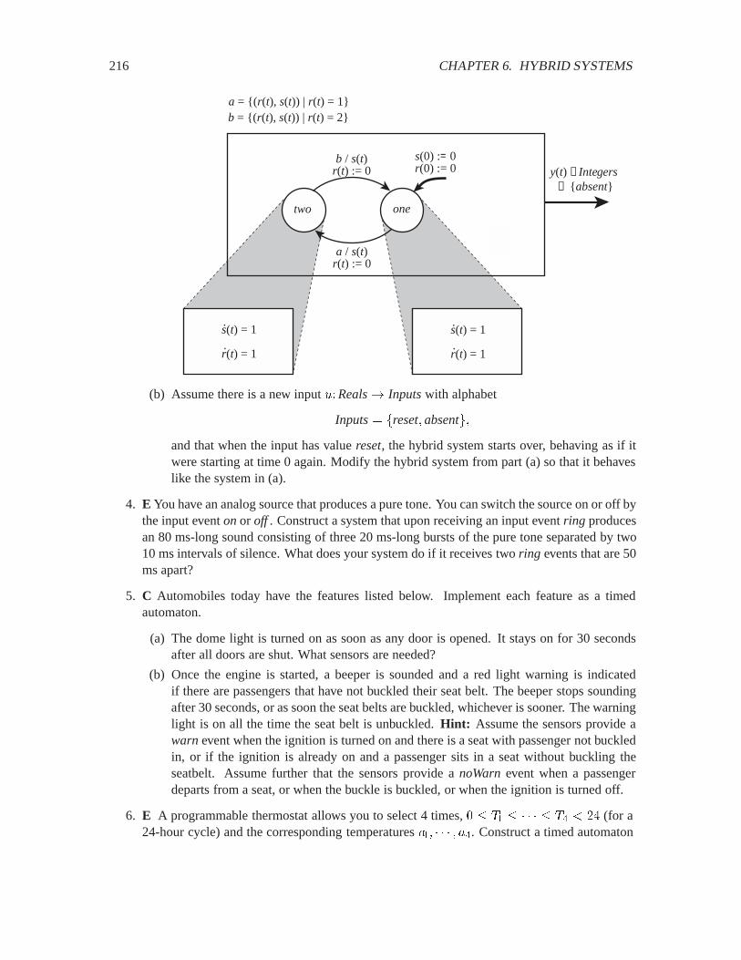
216 CHAPTER 6. HYBRID SYSTEMS
b / s(t)r(t) := 0
two one
a / s(t)r(t) := 0
y(t) ∈Integers ∪ {absent}
s(0) := 0r(0) := 0
b = {(r(t), s(t)) | r(t) = 2}a = {(r(t), s(t)) | r(t) = 1}
s(t) = 1
r(t) = 1
.
.s(t) = 1
r(t) = 1
.
.
(b) Assume there is a new input 0�Reals� Inputswith alphabet
Inputs� �reset�absent�and that when the input has value reset, the hybrid system starts over, behaving as if itwere starting at time 0 again. Modify the hybrid system from part (a) so that it behaveslike the system in (a).
4. E You have an analog source that produces a pure tone. You can switch the source on or off bythe input event onor off . Construct a system that upon receiving an input event ring producesan 80 ms-long sound consisting of three 20 ms-long bursts of the pure tone separated by two10 ms intervals of silence. What does your system do if it receives two ring events that are 50ms apart?
5. C Automobiles today have the features listed below. Implement each feature as a timedautomaton.
(a) The dome light is turned on as soon as any door is opened. It stays on for 30 secondsafter all doors are shut. What sensors are needed?
(b) Once the engine is started, a beeper is sounded and a red light warning is indicatedif there are passengers that have not buckled their seat belt. The beeper stops soundingafter 30 seconds, or as soon the seat belts are buckled, whichever is sooner. The warninglight is on all the time the seat belt is unbuckled. Hint: Assume the sensors provide awarnevent when the ignition is turned on and there is a seat with passenger not buckledin, or if the ignition is already on and a passenger sits in a seat without buckling theseatbelt. Assume further that the sensors provide a noWarnevent when a passengerdeparts from a seat, or when the buckle is buckled, or when the ignition is turned off.
6. E A programmable thermostat allows you to select 4 times, � � � � ) �� (for a24-hour cycle) and the corresponding temperatures ��� � �. Construct a timed automaton
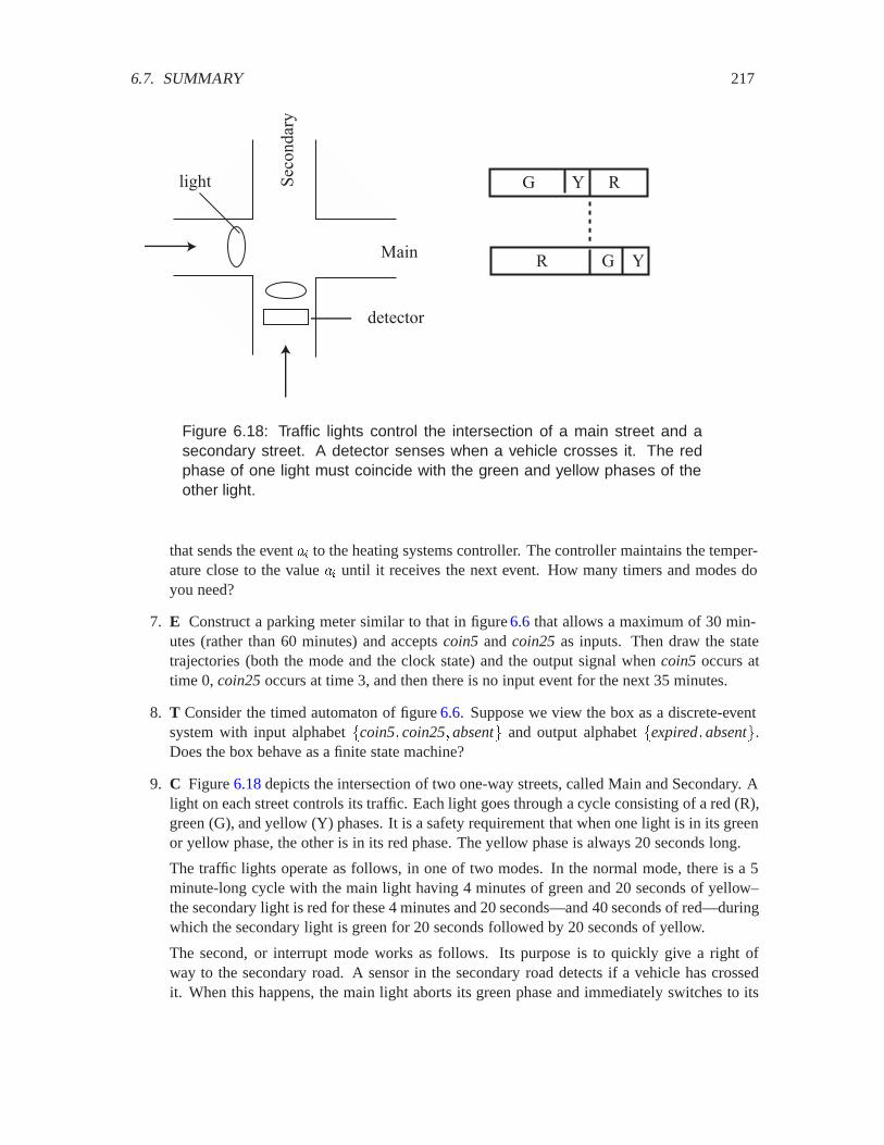
6.7. SUMMARY 217
Main
Seco
ndar
y
light
detector
R
R G
G Y
Y
Figure 6.18: Traffic lights control the intersection of a main street and asecondary street. A detector senses when a vehicle crosses it. The redphase of one light must coincide with the green and yellow phases of theother light.
that sends the event �� to the heating systems controller. The controller maintains the temper-ature close to the value �� until it receives the next event. How many timers and modes doyou need?
7. E Construct a parking meter similar to that in figure 6.6 that allows a maximum of 30 min-utes (rather than 60 minutes) and accepts coin5 and coin25 as inputs. Then draw the statetrajectories (both the mode and the clock state) and the output signal when coin5 occurs attime 0, coin25occurs at time 3, and then there is no input event for the next 35 minutes.
8. T Consider the timed automaton of figure 6.6. Suppose we view the box as a discrete-eventsystem with input alphabet �coin5� coin25�absent and output alphabet �expired�absent.Does the box behave as a finite state machine?
9. C Figure 6.18 depicts the intersection of two one-way streets, called Main and Secondary. Alight on each street controls its traffic. Each light goes through a cycle consisting of a red (R),green (G), and yellow (Y) phases. It is a safety requirement that when one light is in its greenor yellow phase, the other is in its red phase. The yellow phase is always 20 seconds long.
The traffic lights operate as follows, in one of two modes. In the normal mode, there is a 5minute-long cycle with the main light having 4 minutes of green and 20 seconds of yellow–the secondary light is red for these 4 minutes and 20 seconds—and 40 seconds of red—duringwhich the secondary light is green for 20 seconds followed by 20 seconds of yellow.
The second, or interrupt mode works as follows. Its purpose is to quickly give a right ofway to the secondary road. A sensor in the secondary road detects if a vehicle has crossedit. When this happens, the main light aborts its green phase and immediately switches to its
218 CHAPTER 6. HYBRID SYSTEMS
20 second yellow phase. If the vehicle is detected while the main light is yellow or red, thesystem continues in its normal mode.
Design a hybrid system that controls the lights. Let this hybrid system have discrete outputsthat are pairs 99�9$�9�� etc. where the first letter denotes the color of the main lightsecond letter denotes the color of the secondary light.
10. T Design a ReceiverProtocolhybrid system that works together with the SenderProtocolofexample 6.7.
11. E For the bouncing ball of example 6.9 let � be the time when the ball hits the ground forthe �-th time, and let "��� � ����� be the velocity at that time.
(a) Find a relation between "��� � and "��� and then calculate "��� in terms of "��.
(b) Obtain � in terms of "���.
(c) Calculate the maximum height reached by the ball after successive bumps.
12. E Translate refinement systems that are described as second-order differential equations intofirst-order differential equations. Specifically:
(a) For the sticky masses system in example6.8, find the function � such that (6.1) and (6.2)are represented as (6.4). Is this function linear?
(b) For the bouncing ball system in example 6.9, find the function � such that (6.5) isrepresented as (6.6). Is this function linear?
13. T Elaborate the hybrid system model of figure6.12 so that in the togethermode, the stickinessdecays according to the differential equation
���� � �����
where ��� is the stickiness at time , and � is some positive constant. On the transition intothis mode, the stickiness should be initialized to some starting stickiness �.
14. T Show that the trajectory of the AGV of figure 6.15 while it is in left or right mode is acircle. What is the radius of this circle, and how long does it take to complete a circle?
15. E Express the hybrid system of figure 6.15 in terms of the formal model of section 6.6. Thatis, identify the sets Inputs, Outputs, and the TransitionStructure.

Chapter 7
Frequency Domain
We are interested in manipulating signals. We may wish to synthesize signals, as modems needto do in order to transmit a voice-like signal through the telephone channel. We may instead wishto analyze signals, as modems need to do in order to extract digital information from a receivedvoice-like signal. In general, the field of communications is all about synthesizing signals withcharacteristics that match a channel, and then analyzing signals that have often been corrupted bythe channel in order to extract the original information.
We may also wish to synthesize natural signals such as images or speech. The field of computergraphics puts much of its energy into synthesizing natural-looking images. Image processingincludes image understanding, which involves analyzing images to determine their content. Thefield of signal processing includes analysis and synthesis of speech and music signals.
We may wish to control a physical process. The physical process is sensed (using temperature,pressure, position and speed sensors). The sensed signals are processed in order to estimate theinternal state of the physical process. The physical process is controlled on the basis of the stateestimate. Control system design includes the design of state estimators and controllers.
In order to analyze or synthesize signals, we need models of those signals. Since a signal is a func-tion, a model of the signal is a description or a definition of the function. We use two approaches.The first is a declarative (what is) approach. The second is an imperative (how to) approach.These two approaches are complementary. Depending on the situation, one approach is better thanthe other.
Signals are functions. This chapter in particular deals with signals where the domain is time (dis-crete or continuous). It introduces the concept of frequency-domain representation of these signals.The idea is that arbitrary signals can be described as sums of sinusoidal signals. This concept is firstmotivated by referring to psychoacoustics, how humans hear sounds. Sinusoidal signals have par-ticular psychoacoustic significance. But the real justification for the frequency domain approach ismuch broader. It turns out to be particularly easy to understand the effect that LTI systems (lineartime invariant systems), discussed in chapter 5, have on sinusoidal signals. A powerful set ofanalysis and design techniques then follow for arbitrary signals and the LTI systems that operate onthem.
219

220 CHAPTER 7. FREQUENCY DOMAIN
Although we know that few (if any) real-world systems are truly LTI, we can easily construe modelswhere the approximation is valid over some regime of operation. The previous chapter showedhow modal models can be constructed to build realistic models over a broader range of operatingconditions. Frequency domain methods are amenable to such hybrid system treatment.
7.1 Frequency decomposition
For some signals, particularly natural signals like voice, music, and images, finding a concise andprecise definition of the signal can be difficult. In such cases, we try to model signals as composi-tions of simpler signals that we can more easily model.
Psychoacoustics is the study of how humans hear sounds. Pure tones and their frequency turn out tobe a very convenient way to describe sounds. Musical notes can be reasonably accurately modeledas combinations of relatively few pure tones (although subtle properties of musical sounds, such asthe timbre of a sound, are harder to model accurately).
When studying sounds, it is reasonable on psychoacoustic grounds to decompose the sounds intosums of sinusoids. It turns out that the motivation for doing this extends well beyond psychoacous-tics. Pure tones have very convenient mathematical properties that make it useful to model othertypes of signals as sums of sinusoids, even when there is no psychoacoustic basis for doing so. Forexample, there is no psychoacoustic reason for modeling radio signals as sums of sinusoids.
Consider the range of frequencies covering one octave, ranging from 440Hz to 880 Hz. “Octave”is the musical term for a factor of two in frequency. The frequencies 440 Hz and 880 Hz bothcorrespond to the musical note A, but one octave apart. The next higher A in the musical scalewould have the frequency 1760 Hz, twice 880 Hz. In the western musical scale, there are 12 notesin every octave. These notes are evenly distributed (geometrically), so the next note above A, whichis B flat, has frequency �� � ��
��, where ��
�� � ����. The next note above B flat, which is B,
has frequency ��� ����� ��
��.
In table 7.1, the frequencies of the complete musical scale between middle A and A-880 are shown.Each frequency is + � ��
�� times the frequency below it.
Frequencies that are harmonically related tend to sound good together. Figure7.1 shows the graphof a signal that is a major triad, a combination of the notes A, CC (C sharp), and E. By “combination”we mean “sum.” The A is a sinusoidal signal at 440 Hz. It is added to a CC, which is a sinusoidalsignal at 554 Hz. This sum is then added to an E, which is a sinusoidal signal at 659 Hz. Each ofthe components is also shown, so you can verify graphically that at each point in time, the value ofthe solid signal is equal to the sum of values of the dashed signals at that time.
The stimulus presented to the ear is the solid waveform. What you hear, however, assuming a smallamount of musical training, is the three sinusoidal components, which the human ear interprets asmusical notes. The human ear decomposes the stimulus into its sinusoidal components.
Example 7.1: The major triad signal can be written as a sum of sinusoids
��� � ������ � ��� � ������� � ��� � ���� �� � ����
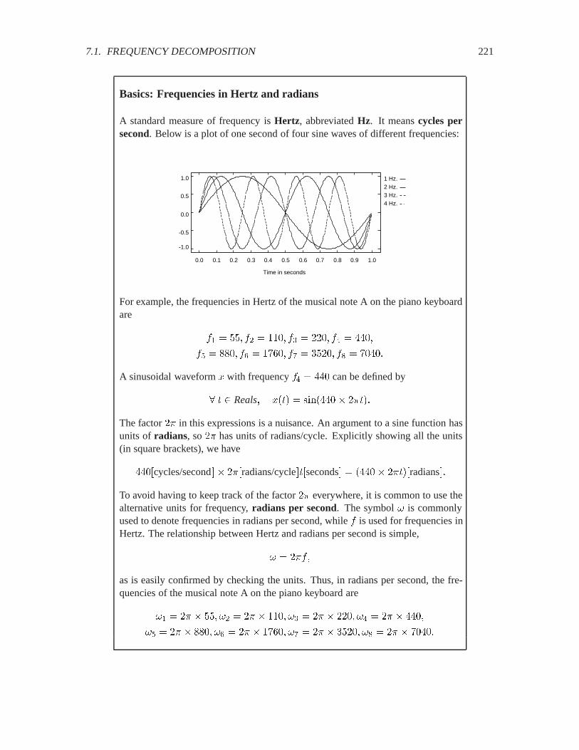
7.1. FREQUENCY DECOMPOSITION 221
Basics: Frequencies in Hertz and radians
A standard measure of frequency is Hertz, abbreviated Hz. It means cycles persecond. Below is a plot of one second of four sine waves of different frequencies:
1 Hz.2 Hz.3 Hz.4 Hz.
-1.0
-0.5
0.0
0.5
1.0
0.0 0.1 0.2 0.3 0.4 0.5 0.6 0.7 0.8 0.9 1.0
Time in seconds
For example, the frequencies in Hertz of the musical note A on the piano keyboardare
�� � ��� �� � � �� � ��� � � ���
�� � ��� �� � � � �� � ���� �� � ���
A sinusoidal waveform � with frequency � � �� can be defined by
� Reals� ��� � ������ � ����
The factor �� in this expressions is a nuisance. An argument to a sine function hasunits of radians, so �� has units of radians/cycle. Explicitly showing all the units(in square brackets), we have
���cycles/second�� ���radians/cycle��seconds� � ��� � ����radians��
To avoid having to keep track of the factor �� everywhere, it is common to use thealternative units for frequency, radians per second. The symbol � is commonlyused to denote frequencies in radians per second, while � is used for frequencies inHertz. The relationship between Hertz and radians per second is simple,
� � ����
as is easily confirmed by checking the units. Thus, in radians per second, the fre-quencies of the musical note A on the piano keyboard are
�� � �� � ��� �� � �� � � �� � �� � ��� � � �� � ���
�� � �� � ��� �� � �� � � � �� � �� � ���� �� � �� � ���
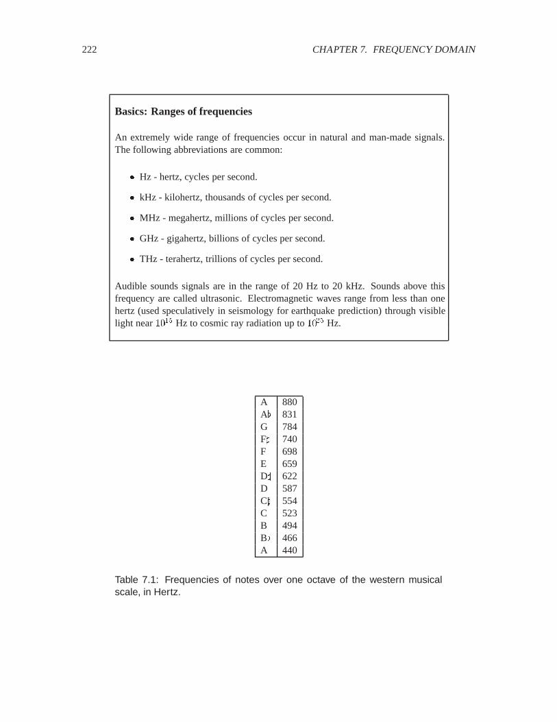
222 CHAPTER 7. FREQUENCY DOMAIN
Basics: Ranges of frequencies
An extremely wide range of frequencies occur in natural and man-made signals.The following abbreviations are common:
� Hz - hertz, cycles per second.
� kHz - kilohertz, thousands of cycles per second.
� MHz - megahertz, millions of cycles per second.
� GHz - gigahertz, billions of cycles per second.
� THz - terahertz, trillions of cycles per second.
Audible sounds signals are in the range of 20 Hz to 20 kHz. Sounds above thisfrequency are called ultrasonic. Electromagnetic waves range from less than onehertz (used speculatively in seismology for earthquake prediction) through visiblelight near �� Hz to cosmic ray radiation up to �� Hz.
A 880AD 831G 784FC 740F 698E 659DC 622D 587CC 554C 523B 494BD 466A 440
Table 7.1: Frequencies of notes over one octave of the western musicalscale, in Hertz.
7.1. FREQUENCY DECOMPOSITION 223
Probing further: Circle of fifths
The western musical scale is based on our perception of frequency and the har-monic relationships between frequencies. The following frequencies all correspondto the note A:
110, 220, 440, 880, 1760, and 3520.
What about �� � � � ��? Notice that ���� � , which is almost exactlythe E in table 7.1. Thus, �� � � is (roughly) the note E, one octave above the Eabove A-440. E and A are closely harmonically related, and to most people, theysound good together. It is because
�� � � � ��� �
The notes A, CC, and E form a major triad. Where does the CC come from? Itsfrequency is 554 (see table 7.1). Notice that
��� � � ��� � ��
Among all the harmonic relationships in the scale, A, CC, and E have one of thesimplest. This is the reason for their pleasing sound together.
For more arcane reasons, the interval between A and E, which is a frequency riseof approximately 3/2, is called a fifth. The note 3/2 (a fifth) above E has frequency988, which is one octave above B-494. Another 3/2 above that is approximatelyF sharp (740 Hz). Continuing in this fashion, multiplying frequencies by 3/2, andthen possibly dividing by two, you can approximately trace the twelve notes of thescale. On the 13-th, you return to A, approximately. This progression is called thecircle of fifths. The notion of key and scale in music are based on this circle offifths, as is the fact that there are 12 notes in the scale.
Table 7.1 is calculated by multiplying each frequency by ���� to get the next higher
frequency, not by using the circle of fifths. Indeed, the ���� method applied twelve
times yields a note that is exactlyone octave higher than the starting point, whilethe circle of fifths only yields an approximation. The ��
�� method yields the well-
tempered scale. This scale was popularized by the composer J. S. Bach. It soundsmuch better than a scale based on the circle fifths when the range of notes spansmore than one octave.

224 CHAPTER 7. FREQUENCY DOMAIN
-3x10
SumA
C sharpE
-2
-1
0
1
2
3
0 1 2 3 4 5 6 7 8
Major Triad
Time in seconds
Figure 7.1: Graph of a major triad, showing its three sinusoidal componentsand their sum.
-3x10
-2
-1
0
1
2
0 1 2 3 4 5 6 7 8 9
Time in seconds
Figure 7.2: A sound waveform for an A-220 with more interesting timbre.
for all Reals. The human ear hears as distinct tones the frequencies of these si-nusoidal components. Musical sounds such as chords can be characterized as sums ofpure tones.
Purely sinusoidal signals, however, do not sound very good. Although they are recognizable asnotes, they do not sound like any familiar musical instrument. Truly musical sounds are much morecomplex than a pure sinusoid. The characteristic sound of an instrument is its timbre, and as weshall see, some aspects of timbre can also be characterized as sums of sinusoids.
Timbre is due in part to the fact that musical instruments do not produce purely sinusoidal sounds.Instead, to a first approximation, they produce sounds that consist of a fundamental sinusoidal com-ponent and harmonics. The fundamental is at the frequency of the note being played, and theharmonics are at multiples of that frequency. Figure7.2 shows a waveform for a sound that is heardas an A-220 but has a much more interesting timbre than a sinusoidal signal with frequency 220Hz. In fact, this waveform is generated by adding together sinusoidal signals with frequencies 220
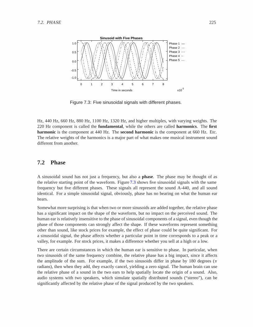
7.2. PHASE 225
-3x10
Phase 1Phase 2Phase 3Phase 4Phase 5
-1.0
-0.5
0.0
0.5
1.0
0 1 2 3 4 5 6 7 8
Sinusoid with Five Phases
Time in seconds
Figure 7.3: Five sinusoidal signals with different phases.
Hz, 440 Hz, 660 Hz, 880 Hz, 1100 Hz, 1320 Hz, and higher multiples, with varying weights. The220 Hz component is called the fundamental, while the others are called harmonics. The firstharmonic is the component at 440 Hz. The second harmonic is the component at 660 Hz. Etc.The relative weights of the harmonics is a major part of what makes one musical instrument sounddifferent from another.
7.2 Phase
A sinusoidal sound has not just a frequency, but also a phase. The phase may be thought of asthe relative starting point of the waveform. Figure 7.3 shows five sinusoidal signals with the samefrequency but five different phases. These signals all represent the sound A-440, and all soundidentical. For a simple sinusoidal signal, obviously, phase has no bearing on what the human earhears.
Somewhat more surprising is that when two or more sinusoids are added together, the relative phasehas a significant impact on the shape of the waveform, but no impact on the perceived sound. Thehuman ear is relatively insensitive to the phase of sinusoidal components of a signal, even though thephase of those components can strongly affect the shape. If these waveforms represent somethingother than sound, like stock prices for example, the effect of phase could be quite significant. Fora sinusoidal signal, the phase affects whether a particular point in time corresponds to a peak or avalley, for example. For stock prices, it makes a difference whether you sell at a high or a low.
There are certain circumstances in which the human ear is sensitive to phase. In particular, whentwo sinusoids of the same frequency combine, the relative phase has a big impact, since it affectsthe amplitude of the sum. For example, if the two sinusoids differ in phase by 180 degrees (�radians), then when they add, they exactly cancel, yielding a zero signal. The human brain can usethe relative phase of a sound in the two ears to help spatially locate the origin of a sound. Also,audio systems with two speakers, which simulate spatially distributed sounds (“stereo”), can besignificantly affected by the relative phase of the signal produced by the two speakers.
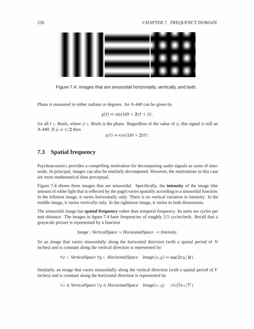
226 CHAPTER 7. FREQUENCY DOMAIN
Figure 7.4: Images that are sinusoidal horizontally, vertically, and both.
Phase is measured in either radians or degrees. An A-440 can be given by
��� � ������ � ��� <��
for all Reals, where < Realsis the phase. Regardless of the value of <, this signal is still anA-440. If < � ��� then
��� � ������ � ����
7.3 Spatial frequency
Psychoacoustics provides a compelling motivation for decomposing audio signals as sums of sinu-soids. In principal, images can also be similarly decomposed. However, the motivations in this caseare more mathematical than perceptual.
Figure 7.4 shows three images that are sinusoidal. Specifically, the intensity of the image (theamount of white light that is reflected by the page) varies spatially according to a sinusoidal function.In the leftmost image, it varies horizontally only. There is no vertical variation in intensity. In themiddle image, it varies vertically only. In the rightmost image, it varies in both dimensions.
The sinusoidal image has spatial frequency rather than temporal frequency. Its units are cycles perunit distance. The images in figure 7.4 have frequencies of roughly 2.5 cycles/inch. Recall that agrayscale picture is represented by a function
Image� VerticalSpace� HorizontalSpace� Intensity�
So an image that varies sinusoidally along the horizontal direction (with a spatial period of ;inches) and is constant along the vertical direction is represented by
�� VerticalSpace�� HorizontalSpace Image��� �� � ��������;��
Similarly, an image that varies sinusoidally along the vertical direction (with a spatial period of Einches) and is constant along the horizontal direction is represented by
�� VerticalSpace�� HorizontalSpace Image��� �� � ��������E ��
7.4. PERIODIC AND FINITE SIGNALS 227
An image that varies sinusoidally along both directions is represented by
�� VerticalSpace�� HorizontalSpace Image��� �� � ��������E �� ��������;��
These sinusoidal images have much less meaning than audio sinusoids, which we perceive as musi-cal tones. Nonetheless, we will see that images can be described as sums of sinusoids, and that suchdescription is sometimes useful.
7.4 Periodic and finite signals
When the domain is continuous or discrete time, we can define a periodic signal. Assuming thedomain is Reals, a periodic signal � with period ( Realsis one where for all Reals
��� � ��� (�� (7.1)
A signal with period ( also has period �(, since
��� � ��� (� � ��� �(��
In fact, it has period >(, for any positive integer > . Usually, we define the period to be the smallest( 2 such that
� Reals� ��� � ��� (��
Example 7.2: The sinusoidal signal � where for all Reals
��� � �������
is a periodic signal with period ����� since for all Reals
�������� ������� � ��������
A periodic signal is defined over an infinite interval. If the domain is instead a subset ��� �� � Reals,for some finite � and �, then we call this a finite signal.
Example 7.3: The signal � where for all �� ������,
��� � �������
is a finite signal with duration �����. This interval spans exactly one cycle of the sinewave.
A finite signal with duration ( can be used to define a periodic signal with period (. All that isneeded is to periodically repeat the finite signal. Formally, given a finite signal �� ��� �� � Reals,we can define a signal ���Reals� Realsby
� Reals� ���� �
���� if ��� �� otherwise
(7.2)

228 CHAPTER 7. FREQUENCY DOMAIN
In other words, ���� is simply ��� inside its domain, and zero elsewhere. Then the periodic signalcan be given by1
��� ���
��������'(� (7.3)
where ( � �� �. This is called a shift-and-add summation, illustrated in figure 7.5. The periodicsignal is a sum of versions of ���� that have been shifted in time by multiples of (. Do not let theinfinite sum intimidate: all but one of the terms of the summation are zero for any fixed ! Thus, aperiodic signal can be defined in terms of a finite signal, which represents one period. Conversely,a finite signal can be defined in terms of a periodic signal (by taking one period).
We can check that � given by (7.3) is indeed periodic with period (,
��� (� ���
����
���� (�'(� ���
����
���� �'� �(�
���
����
���� 6(� � ����
by using a change of variables, 6 � '� .
It is also important to note that the periodic signal � agrees with � in the finite domain ��� �� of �,since
� ��� �� ��� ���
����
����'(�
� ���� ������
����'(�
� ����
because, by (7.2), for ��� ��, ���� � ��� and ����'(� � if ' �� .
We will see that any periodic signal, and hence any finite signal, can be described as a sum ofsinusoidal signals. This result, known as the Fourier series, is one of the fundamental tools in thestudy of signals and systems.
7.5 Fourier series
A remarkable result, due to Joseph Fourier, 1768-1830, is that a periodic signal ��Reals� Realswith period ( Realscan (usually) be described as a constant term plus a sum of sinusoids,
��� � �� ������
�� ����6��� <�� (7.4)
This representation of � is called its Fourier series. The Fourier series is widely used for signalanalysis. Each term in the summation is a cosine with amplitude �� and phase <�. The particular
1If this notation is unfamiliar, see box on page 63.

7.5. FOURIER SERIES 229
y'(t + p)
t
t
t
t
x(t)
t
y'(t)
p
y'(t − p)
y'(t − 2p)
a b
......
Σ
p
Figure 7.5: By repeating the finite signal � we can obtain a periodic signal�.
230 CHAPTER 7. FREQUENCY DOMAIN
values of �� and <� depend on �, of course. The frequency ��, which has units of radians persecond (assuming the domain of � is in seconds), is called the fundamental frequency, and isrelated to the period ( by
�� � ���(�
In other words, a signal with fundamental frequency �� has period ( � ����. The constant term�� is sometimes called the DC term, where “DC” stands for direct current, a reference back tothe early applications of this theory in electrical circuit analysis. The terms where 6 � � are calledharmonics.
Equation (7.4) is often called the Fourier series expansion for � because it expands � in terms ofits sinusoidal components.
If we had a facility for generating individual sinusoids, we could use the Fourier series represen-tation (7.4) to synthesize any periodic signal. However, using the Fourier series expansion forsynthesis of periodic signals is problematic because of the infinite summation. But for most practi-cal signals, the coefficients �� become very small (or even zero) for large 6, so a finite summationcan be used as an approximation. A finite Fourier series approximation with > � terms has theform
"��� � �� ������
�� ����6��� <��� (7.5)
The infinite summation of (7.4) is, in fact, the limit of (7.5) as > goes to infinity. We need to beconcerned, therefore, with whether this limit exists. The Fourier series expansion is valid only if itexists. There are some technical mathematical conditions on � that, if satisfied, ensure that the limitexists (see boxes on pages 234 and 235). Fortunately, these conditions are met almost always bypractical, real-world time-domain signals.
Example 7.4: Figure 7.6 shows a square wave with period 8 msec and some finiteFourier series approximations to the square wave. Only one period of the square waveis shown. The method for constructing these approximations will be covered in detailin chapter 10. Here, we will just observe the general structure of the approximations.
Notice in figure 7.6(a) that the > � approximation consists only of the DC term(which is zero in this case) and a sinusoid with an amplitude slightly larger than that ofthe square wave. Its amplitude is depicted in figure 7.6(b) as the height of the largestbar. The horizontal position of the bar corresponds to the frequency of the sinusoid,125 Hz, which is 1/(8 msec), the fundamental frequency. The > � � waveform is thesum of the > � waveform and one additional sinusoid with frequency 375 Hz andamplitude equal to the height of the second largest bar in figure7.6(b).
A plot like that in figure 7.6(b) is called a frequency domain representation of the square wave,because it depicts the square wave by the amplitude and frequency of its sinusoidal components. Ac-tually, a complete frequency domain representation also needs to give the phase of each sinusoidalcomponent.

7.5. FOURIER SERIES 231
-3x10
idealK=1
K = 3K = 7
K = 32
-1.0
-0.5
0.0
0.5
1.0
0 1 2 3 4 5 6 7 8
Time in seconds
(a)
3x10
0.00.2
0.4
0.6
0.8
1.0
1.2
0.0 0.5 1.0 1.5 2.0 2.5 3.0 3.5 4.0
Frequency in Hz
(b)
Figure 7.6: (a) One cycle of a square wave and some finite Fourier se-ries approximations. (b) The amplitudes of the Fourier series terms for thesquare wave.
232 CHAPTER 7. FREQUENCY DOMAIN
Notice in figure 7.6(b) that all even terms of the Fourier series approximation have zero amplitude.Thus, for example, there is no component at 250 Hz. This is a consequence of the symmetry of thesquare wave, although it is beyond the scope of work now to explain exactly why.
Also notice that as the number of terms in the summation increases, the approximation more closelyresembles a square wave, but the amount of its overshoot does not appear to decrease. This is knownas Gibb’s phenomenon. In fact, the maximum difference between the finite Fourier series approx-imation and the square wave does not converge to zero as the number of terms in the summationincreases. In this sense, the square wave cannot be exactly described with a Fourier series (see boxon page 234). Intuitively, the problem is due to the abrupt discontinuity in the square wave when ittransitions between its high value and its low value. In another sense, however, the square wave isaccurately described by a Fourier series. Although the maximum difference between the approxi-mation and the square wave does not go to zero, the mean square errordoes go to zero (see box onpage 235). For practical purposes, mean square error is an adequate criterion for convergence, sowe can work with the Fourier series expansion of the square wave.
Example 7.5: Figure 7.7 shows some finite Fourier series approximations for a trian-gle wave. This waveform has no discontinuities, and therefore the maximum error inthe finite Fourier series approxination converges to zero (see box on page234). Noticethat its Fourier series components decrease in amplitude much more rapidly than thoseof the square wave. Moreover, the time-domain approximations appear to be moreaccurate with fewer terms in the finite summation.
Many practical, real-world signals, such as audio signals, do not have discontinuities, and thus donot exhibit the sort of convergence problems exhibited by the square wave (Gibbs phenomenon).Other signals, however, such as images, are full of discontinuities. A (spatial) discontinuity in animage is simply an edge. Most images have edges. Nonetheless, a Fourier series representation forsuch a signal is almost always still valid, in a mean square error sense (see box on page235). Thisis sufficient for almost all engineering purposes.
Example 7.6: Consider an audio signal given by
��� � ������ � ��� � ������ � ��� � ���� � ����
This is a major triad in a non-well-tempered scale. The first tone is A-440. The third isapproximately E, with a frequency 3/2 that of A-440. The middle term is approximatelyCC, with a frequency 5/4 that of A-440. It is these simple frequency relationships thatresult in a pleasant sound. We choose the non-well-tempered scale because it makesit much easier to construct a Fourier series expansion for this waveform. We leave themore difficult problem of finding the Fourier series coefficients for a well-temperedmajor triad to exercise 5.
To construct the Fourier series expansion, we can follow these steps:
1. Find (, the period. The period is the smallest number ( 2 such that ��� ���� (� for all in the domain. To do this, note that
�������� � ��������� (��
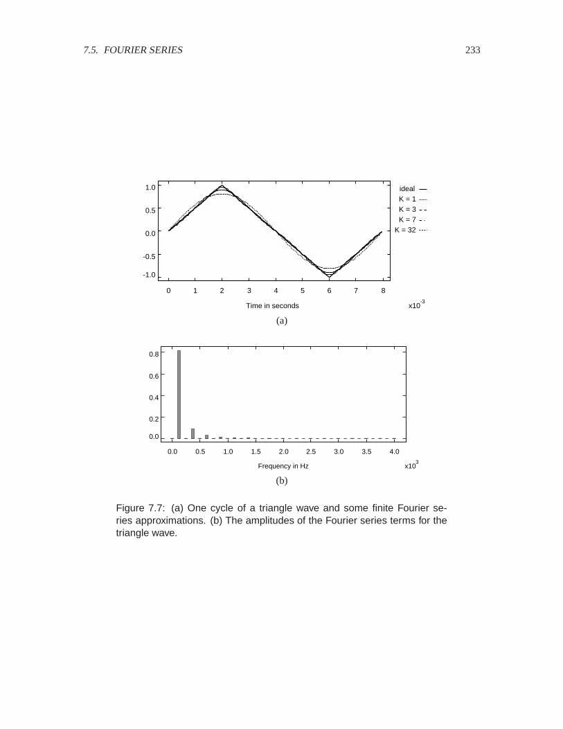
7.5. FOURIER SERIES 233
-3x10
idealK = 1K = 3K = 7
K = 32
-1.0
-0.5
0.0
0.5
1.0
0 1 2 3 4 5 6 7 8
Time in seconds
(a)
3x10
0.0
0.2
0.4
0.6
0.8
0.0 0.5 1.0 1.5 2.0 2.5 3.0 3.5 4.0
Frequency in Hz
(b)
Figure 7.7: (a) One cycle of a triangle wave and some finite Fourier se-ries approximations. (b) The amplitudes of the Fourier series terms for thetriangle wave.

234 CHAPTER 7. FREQUENCY DOMAIN
Probing further: Uniform convergence of the Fourier series
The Fourier series representation of a periodic signal � is a limit of a sequence offunctions �� for � � � �� where
� Reals� �� �� � �� ������
�� ����6��� <���
Specifically, for the Fourier series representation to be valid, we would like that forall Reals,
��� � !����
�� ���
A strong criterion for validity of the Fourier series is uniform convergence of thislimit, in which for each real number A 2 , there exists a positive integer 3 suchthat for all Realsand for all � 2 3 ,
����� �� ��� ) A
A sufficient condition for uniform convergence is that the signal � be continuousand that its first derivative be piecewise continuous.
A square wave, for example, is not continuous, and hence does not satisfy thissufficient condition. Indeed, the Fourier series does not converge uniformly, asyou can see in figure 7.6 by observing that the peak difference between ��� and���� does not decrease to zero. A triangle wave, however, is continuous, and has apiecewise continuous first derivative. Thus, it does satisfy the sufficient condition.Its Fourier series approximation will therefore converge uniformly, as suggested infigure 7.7. A weaker, but still useful, criterion for validity of the Fourier series isconsidered on page 235. That criterion is met by the square wave.
See for example R. G. Bartle, The Elements of Real Analysis, Second Edition,John Wiley & Sons, 1976, p. 117 (for uniform convergence) and p. 337 (for thissufficient condition).
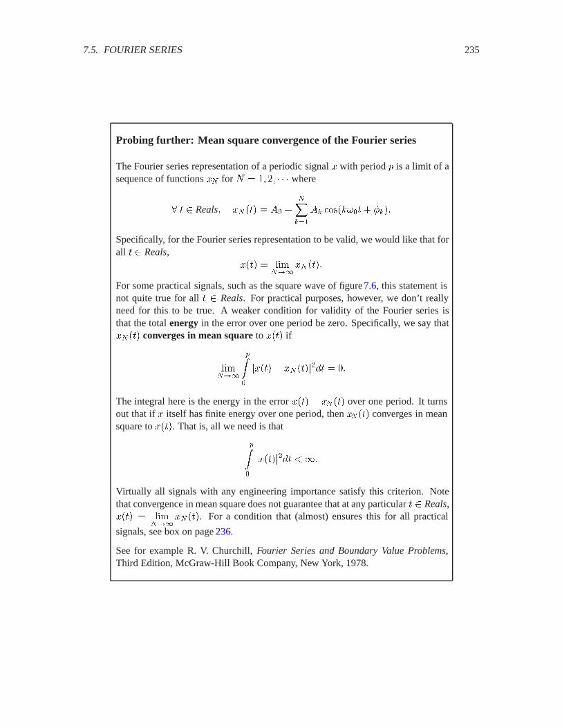
7.5. FOURIER SERIES 235
Probing further: Mean square convergence of the Fourier series
The Fourier series representation of a periodic signal � with period ( is a limit of asequence of functions �� for � � � �� where
� Reals� �� �� � �� ������
�� ����6��� <���
Specifically, for the Fourier series representation to be valid, we would like that forall Reals,
��� � !����
�� ���
For some practical signals, such as the square wave of figure7.6, this statement isnot quite true for all Reals. For practical purposes, however, we don’t reallyneed for this to be true. A weaker condition for validity of the Fourier series isthat the total energy in the error over one period be zero. Specifically, we say that�� �� converges in mean square to ��� if
!����
#��
����� �� ����� � �
The integral here is the energy in the error ��� � �� �� over one period. It turnsout that if � itself has finite energy over one period, then �� �� converges in meansquare to ���. That is, all we need is that
#��
������� )��
Virtually all signals with any engineering importance satisfy this criterion. Notethat convergence in mean square does not guarantee that at any particular Reals,��� � !��
���� ��. For a condition that (almost) ensures this for all practical
signals, see box on page 236.
See for example R. V. Churchill, Fourier Series and Boundary Value Problems,Third Edition, McGraw-Hill Book Company, New York, 1978.

236 CHAPTER 7. FREQUENCY DOMAIN
Probing further: Dirichlet conditions for validity of the Fourier series
The Fourier series representation of a periodic signal � with period ( is a limit ofa sequence of finite Fourier series approximations �� for � � � �� . We haveseen in the box on page 234 a strong condition that ensures that � Reals,
��� � !����
�� ��� (7.6)
We have seen in the box on page 235 a weaker condition that does not guaranteethis, but instead guarantees that the energy in the error over one period is zero. Itturns that for almost all signals of interest, we can assert that (7.6) holds for almostall Reals. In particular, if the Dirichlet conditions are satisfied, then (7.6)holds for all except where � is discontinuous. The Dirichlet conditions are three:
� Over one period, � is absolutely integrable, meaning that
#��
������ )��
� Over one period, � is of bounded variation, meaning that there are no morethan a finite number of maxima or minima. That is, if the signal is oscillatingbetween high and low values, it can only oscillate a finite number of times ineach period.
� Over one period, � is continuous at all but a finite number of points.
These conditions are satisfied by the square wave, and indeed by any signal ofpractical engineering importance.
7.5. FOURIER SERIES 237
if �( is an integer. Thus, we want to find the smallest ( such that ��(, ��(,and ( are all integers. Equivalently, we want to find the largest fundamentalfrequency �� � �( such that �����, �����, and ��� are all integers. Suchan �� is called the greatest common divisor of 440, 550, and 660. This can becomputed using the gcd function in Matlab. In this case, however, we can do itin our heads, observing that �� � .
2. Find ��, the constant term. By inspection, there is no constant component in ���,only sinusoidal components, so �� � .
3. Find ��, the fundamental term. By inspection, there is no component at 110 Hz,so �� � . Since �� � , <� is immaterial.
4. Find ��, the first harmonic. By inspection, there is no component at 220 Hz, so�� � .
5. Find ��. By inspection, there is no component at 330 Hz, so �� � .
6. Find �. There is a component at 440 Hz, ������ � ���. We need to find �and < such that
� ������ � ��� <� � ������ � ����
By inspection, < � ���� and � � .
7. Similarly determine that �� � �� � , <� � <� � ����, and that all otherterms are zero.
Putting this all together, the Fourier series expansion can be written
��� ���
��
����6��� ����
where �� � ���� � ���.
Clearly the method used in the above example for determining the Fourier series coefficients istedious and error prone, and will only work for simple signals. We will see much better techniquesin chapters 8 and 10.
7.5.1 Uniqueness of the Fourier series
Suppose ��Reals� Realsis a periodic function with period (. Then the Fourier series expansionis unique. In other words if it is both true that
��� � �� ������
�� ����6��� <��
and
��� � �� ������
�� ����6��� #���

238 CHAPTER 7. FREQUENCY DOMAIN
where �� � ���(, then it must also be true that
� 6 � � �� � �� and <� mod �� � #� mod ���
(The modulo operation is necessary because of the non-uniqueness of phase.) Thus, when we talkabout the frequency content of a signal, we are talking about something that is unique and welldefined. For a suggestion about how to prove this uniqueness, see problem11.
7.5.2 Periodic, finite, and aperiodic signals
We have seen in section 7.4 that periodic signals and finite signals have much in common. One canbe defined in terms of the other. Thus, a Fourier series can be used to describe a finite signal aswell as a periodic one. The “period” is simply the extent of the finite signal. Thus, if the domainof the signal is ��� �� � Reals, then ( � � � �. The fundamental frequency, therefore, is just�� � ����� � ��.
An aperiodic signal, like an audio signal, can be partitioned into finite segments, and a Fourier seriescan be constructed from each segment.
Example 7.7: Consider the train whistle shown in figure 7.8(a). Figure 7.8(b) showsa segment of 16 msec. Notice that within this segment, the sound clearly has a some-what periodic structure. It is not hard to envision how it could be described as sums ofsinusoids. The magnitudes of the �� Fourier series coefficients for this 16 msec seg-ment are shown in figure 7.8(c). These are calculated on a computer using techniqueswe will discuss later, rather than being calculated by hand as in the previous example.Notice that there are three dominant frequency components that give the train whistleits tonality and timbre.
7.5.3 Fourier series approximations to images
Images are invariably finite signals. Given any image, it is possible to construct a periodic image byjust tiling a plane with the image. Thus, there is again a close relationship between a periodic imageand a finite one.
We have seen sinusoidal images (figure 7.4), so it follows that it ought to be possible to construct aFourier series representation of an image. The only hard part is that images have a two-dimensionaldomain, and thus are finite in two distinct dimensions. The sinusoidal images in figure7.4 have avertical frequency, a horizontal frequency, or both.
Suppose that the domain of an image is ��� �� � �!� �� � Reals� Reals. Let (& � � � �, and(' � � � ! represent the horizontal and vertical “periods” for the equivalent periodic image. Forconstructing a Fourier series representation, we can define the horizontal and vertical fundamentalfrequencies as follows:
�& � ���(&
�' � ���('

7.5. FOURIER SERIES 239
-0.4
-0.2
0.0
0.2
0.4
0.0 0.2 0.4 0.6 0.8 1.0 1.2 1.4 1.6Time in seconds
(a)
-2x10
-0.2
-0.1
0.0
0.1
0.2
0.0 0.2 0.4 0.6 0.8 1.0 1.2 1.4 1.6
(b)
3x10
0.00
0.02
0.04
0.06
0.08
0.10
0.0 0.5 1.0 1.5 2.0 2.5 3.0 3.5 4.0
(c)
Figure 7.8: (a) A 1.6 second train whistle. (b) A 16 msec segment of thetrain whistle. (c) The Fourier series coefficients for the 16 msec segment.
240 CHAPTER 7. FREQUENCY DOMAIN
The Fourier series representation of Image� ��� �� � �!� ��� �����&� is
Image��� �� ������
�����
���� ����6�&�� <�� ����'�' � � F��
For convenience, we have included the constant term ���� in the summation, so we assume that<� � F� � . (Recall that ����� � ).
7.6 Discrete-time signals
Consider signals of the form �� Integers� Reals, which if the domain is interpreted as time arediscrete-time signals. Discrete-time signals can be decomposed into sinusoidal components muchlike continuous-time signals. There are some minor subtleties, however.
7.6.1 Periodicity
A discrete-time signal is periodic if there is a non-zero integer ( 2 such that
� � Integers� ���� (� � �����
Note that, somewhat counterintuitively, not all sinusoidal discrete-time signals are periodic. Con-sider
���� � !4�������� (7.7)
For this to be periodic, we must be able to find a non-zero integer ( such that for all integers �,
���� (� � !4������� ���(� � !4������� � �����
This can be true only if ����(� is an integer multiple of ��. That is, if there is some integer ' suchthat
���( � ��'�
Dividing both sides by ��(, we see that this signal is periodic only if we can find nonzero integers( and ' such that
� � '�(�
In other words, � must be rational. Only if � is rational is this signal periodic.
Example 7.8: Consider a discrete-time sinusoid � given by
� � Integers� ���� � �����������
Putting this into the form of (7.7),
���� � ��������������
7.6. DISCRETE-TIME SIGNALS 241
Basics: Discrete-time frequencies
When the domain of a signal is Integers, then the units of frequency are cy-cles/sample. Consider for example the discrete-time signal given by
�� Integers� ���� � !4��������
Suppose this represents an audio signal that is sampled at 8000 samples/second.Then to convert � to Hertz, just watch the units:
� �!�!,�����'(,��� ����'(,�����!4��� � �� �!�!,�����!4����
The frequency could have been equally well given in units of radians/sample, as in
���� � !4������
for all � Integers. To convert � to Hertz,
�����&������'(,��� ����'(,�����!4��� � ������!�!,������&���
� ��/�����!�!,�����!4����
we see that it has frequency � � ��� cycles/sample. If this were a continuous-timesinusoid, we could invert this to get the period. However, the inverse is not an integer,so it cannot possibly be the period. Noting that the inverse is 5/2 samples/cycle, weneed to find the smallest multiple of this that is an integer. Multiply by 2, we get 5samples/(2 cycles). So the period is ( � � samples.
In general, for a discrete sinusoid with frequency � cycles/sample, the period is ( � >�� , where> 2 is the smallest integer such that >�� is an integer.
7.6.2 The discrete-time Fourier series
Assume we are given a periodic discrete-time signal � with period (. Just as with continuous-timesignals, this signal can be described as a sum of sinusoids, called the discrete-time Fourier series(DFS) expansion,
���� � �� ������
�� ����6���� <�� (7.8)
where
> �
��(� ��� if ( is odd(�� if ( is even
242 CHAPTER 7. FREQUENCY DOMAIN
Unlike the continuous-time case, the sum is finite. Intuitively, this is because discrete-time signalscannot represent frequencies above a certain value. We will examine this phenomenon in moredetail in chapter 11, but for now, it proves extremely convenient. Mathematically, the above relationis much simpler than the continuous-time Fourier series. All computations are finite. There is afinite number of signal values in one period of the waveform. There is a finite number of terms inthe Fourier series representation for each signal value. Unlike the continuous-time case, it is easyfor computers to manage this representation. Given a finite set of values, ��� � �� , a computercan calculate ����. Moreover, the representation is exact for any periodic signal. No approximationis needed, and there is no question of convergence. In the continuous-time case, the Fourier seriesrepresentation is accurate only for certain signals. For the discrete-time case, it is always accurate.
The DFS can be calculated efficiently on a computer using an algorithm called the fast Fouriertransform (FFT). All of the Fourier series examples that are plotted in this text were calculatedusing the FFT algorithm.
7.7 Summary
A time-based signal can be described as a sum of sinusoids. This sum is called a Fourier series.The magnitudes and phases of the sinusoids, taken together as a function of frequency, are calledthe frequency-domain representation of the signal. For audio signals, this frequency-domain rep-resentation has a direct psychoacoustic significance. But we will see in the next chapter that thisrepresentation has a significance for all signals when LTI systems are used to process the signals.We will see that the effect that an LTI system has on a signal is particularly easy to understand inthe frequency domain.
Exercises
Note: each problem is annotated with the letter E, T, C which stands for exercise, requires somethought, requires some conceptualization. Problems labeled E are usually mechanical, those labeledT require a plan of attack, those labeled C usually have more than one defensible answer.
1. E In (7.1) we defined periodic for continuous-time signals.
(a) Define finite and periodic for discrete-time signals, where the domain is Integers.
(b) Define finite and periodic for images.
2. E Which of the following signals is periodic with a period greater than zero, and what is thatperiod? All functions are of the form ��Reals� Complex. The domain is time, measured inseconds, and so the period is in seconds.
(a) � Reals� ��� � ������� � � � �&� �������
(b) � Reals� ��� � ������� � ��������
(c) � Reals� ��� � ��������� � ����
����
7.7. SUMMARY 243
3. E Consider the discrete-time signal � where
� � Integers� ���� � � �����������
(a) Find the period (, where ( 2 .
(b) Give the fundamental frequency corresponding to the period in (1). Give the units.
(c) Give the coefficients ��� ��� ��� and <�� <�� of the Fourier series expansion forthis signal.
4. E Consider a continuous-time signal ��Reals� Realsdefined by
� Reals� ��� � ������� � ��������
where �� � �� and �� � �� radians/second.
(a) Find the smallest period ( Reals�, where ( 2 .
(b) Give the fundamental frequency corresponding to the period in (a). Give the units.
(c) Give the coefficients ��� ��� ��� and <�� <�� of the Fourier series expansion for�.
5. T Determine the fundamental frequency and the Fourier series coefficients for the well-tempered major triad,
��� � ������ � ��� � ������� � ��� � ���� �� � ����
6. E Define ��Reals� Reals
� Reals� ��� � � ������� ���� � � ������� �� � � � ������� ������
Find � and < so that� Reals� ��� � � ������� <��
Hint: Appendix B might be useful.
7. T In this problem, we examine a practical application of the mathematical result in problem6.In particular, we consider multipath interference, a common problem with wireless systemswhere multiple paths from a transmitter to a receiver can result in destructive interference ofa signal.
When a transmitter sends a radio signal to a receiver, the received signal consists of the directpath plus several reflected paths. In figure 7.9, the transmitter is on a tower at the left of thefigure, the receiver is the telephone in the foreground, and there are three paths: the directpath is ,� meters long, the path reflected from the hill is ,� meters long, and the path reflectedfrom the building is ,� meters long.
Suppose the transmitted signal is a � Hz sinusoid ��Reals� Reals,
� Reals� ��� � � ��������
244 CHAPTER 7. FREQUENCY DOMAIN
So the received signal is � such that � Reals,
��� � *�� ��������� ,�!�� � *�� ��������� ,�
!�� � *�� ��������� ,�
!��� (7.9)
Here, � *� � are numbers that represent the attenuation (or reduction in signal amplitude)of the signal, and ! � � � � m/s is the speed of light in a vacuum.2 Answer the followingquestions.
(a) Explain why the description of � given in (7.9) is a reasonable model of the receivedsignal.
(b) What would be the description if instead of the 3 paths as shown in figure 7.9, therewere 10 paths (one direct and 9 reflected).
(c) The signals received over the different paths cause different phase shifts, <�, so thesignal � (with three paths) can also be written as
� Reals� ��� ���
���
*�� �������� <��
What are the <�? Give an expression in terms of � , ,�, and !.
(d) Let # � ��$�<� � <�� <� � <� be the largest difference in the phase of the receivedsignals and let 1 � ��$�,�� ,�� ,�� ,� be the maximum path length difference. Whatis the relationship between #� 1� �?
(e) Suppose for simplicity that there is only one reflected path of distance ,�, i.e. take*� � in the expressions above. Then # � <� � <�. When # � �, the reflected signalis said to destroythe direct signal. Explain why the term “destroy” is appropriate. (Thisphenomenon is called destructive interference.)
(f) In the context of mobile radio shown in the figure, typically 1 � �m. For what valuesof � is # � ��? (Note that if # � �� the signals will not interact destructively bymuch.)
(g) For the two-path case, derive an expression that relates the frequencies � that interferedestructively to the path length difference 1 � ,� � ,�.
8. T The function ��Reals� Realsis given by its graph shown in figure 7.10. Note that� � �� �� ��� � , and ����� � . Define � by
� Reals� ��� ���
����
��� 6(�
where ( is the period.
(a) Prove that � is periodic with period (, i.e.
� Reals� ��� � ��� (��
2In reality, the reflections are more complicated than the model here.
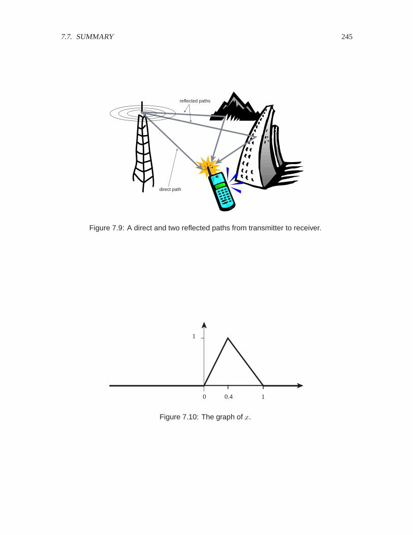
7.7. SUMMARY 245
reflected paths
direct path
Figure 7.9: A direct and two reflected paths from transmitter to receiver.
1
0 0.4 1
Figure 7.10: The graph of �.
246 CHAPTER 7. FREQUENCY DOMAIN
(b) Plot � for ( � .
(c) Plot � for ( � �.
(d) Plot � for ( � ��.
(e) Plot � for ( � ��.
(f) Suppose the function � is obtained by advancing � by 0.4, i.e.
� Reals� ��� � ��� ����
Define / by
� Reals� /�� ���
����
��� 6(�
What is the relation between / and �. Use this relation to plot / for ( � .
9. T Suppose ��Reals� Realsis a periodic signal with period (, i.e.
� Reals� ��� � ��� (��
Let � �Reals� Realsbe any function, and define the signal ��Reals� Realsby � � � Æ �,i.e.
� Reals� ��� � �������
(a) Prove that � is periodic with period (.
(b) Suppose � Reals� ��� � �������. Suppose � is the sign function, � � Reals,
���� �
� if � � � if � )
Plot � and �.
(c) Suppose � Reals� ��� � �������. Suppose � is the square function, � � Reals,���� � ��. Plot �.
10. C Suppose the periodic square wave shown on the left in Figure 7.11 has the Fourier seriesrepresentation
�� ������
�� ������6�(� <��
Use this to obtain a Fourier series representation of the two-dimensional pattern of rectangleson the right.
11. T Suppose �� Complex, �� Reals, and 6 � � �, such that
� Reals� ������� � ���
����� (7.10)
Show that �� � �� and �� � ��. Hint: Evaluate both sides of (7.10) at � , and evaluatetheir derivatives at � .
Discussion: This result shows that in order for two complex exponential signals to be equal,their frequencies, phases, and amplitudes must be equal. More interestingly, this result can

7.7. SUMMARY 247
p
2p/3 2p/3 p
p
2p/3
Figure 7.11: A periodic square wave (left) and a periodic pattern (right).
be used to show that if a signal can be described as a sum of complex exponential signals,then that description is unique. There is no other sum of complex exponentials (one involvingdifferent frequencies, phases, or amplitudes) that will also describe the signal. In particular,the Fourier series representation of a periodic signal is unique, as stated above in theorem7.5.1.

248 CHAPTER 7. FREQUENCY DOMAIN
Chapter 8
Frequency Response
A class of systems that yield to sophisticated analysis techniques is the class of linear time-invariant systems (LTI system), discussed in chapter 5. LTI systems have a key property: givena sinusoidal input, the output is a sinusoidal signal with the same frequency, but possibly differentamplitude and phase. Given an input that is a sum of sinusoids, the output will be a sum of the samesinusoids, each with its amplitude and phase (possibly) modified.
We can justify describing audio signals as sums of sinusoids on purely psychoacoustic grounds.However, because of this property of LTI systems, it is often convenient to describe any signal as asum of sinusoids, regardless of whether there is a psychoacoustic justification. The real value in thismathematical device is that by using the theory of LTI systems, we can design systems that operatemore-or-less independently on the sinusoidal components of a signal. For example, abrupt changesin the signal value require higher frequency components. Thus, we can enhance or suppress theseabrupt changes by enhancing or suppressing the higher frequency components. Such an operationis called filtering because it filters frequency components. We design systems by crafting theirfrequency response, their response to sinusoidal inputs. An audio equalizer, for example, is a filterthat enhances or suppresses certain frequency components. Images can also be filtered. Enhancingthe high frequency components will sharpen the image, whereas suppressing the high frequencycomponents will blur the image.
State-space models described in previous chapters are precise and concise, but in a sense, not aspowerful as a frequency response. For an LTI system, given a frequency response, you can assert agreat deal about the relationship between an input signal and an output signal. Fewer assertions arepractical in general with state-space models.
LTI systems, in fact, can also be described with state-space models, using difference equations anddifferential equations, as explored in chapter 5. But state-space models can also describe systemsthat are not LTI. Thus, state-space models are more general. It should come as no surprise that theprice we pay for this increased generality is fewer analysis and design techniques. In this chapter,we explore the (very powerful) analysis and design techniques that apply to the special case of LTIsystems.
249
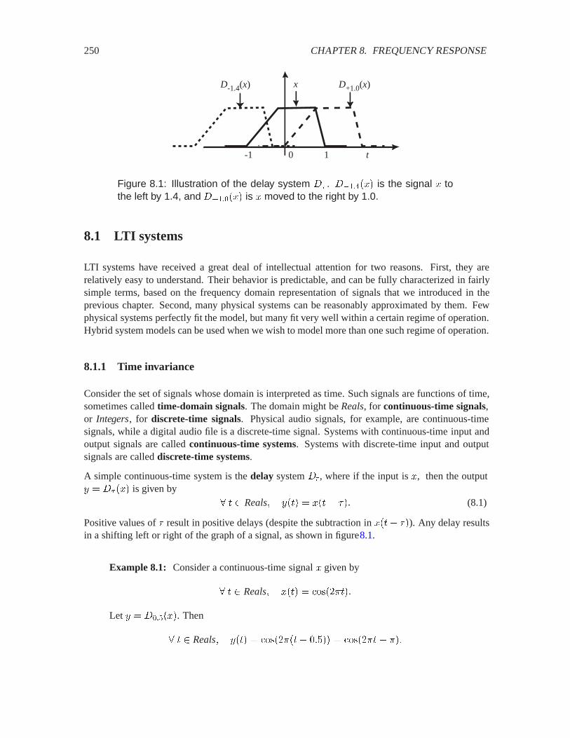
250 CHAPTER 8. FREQUENCY RESPONSE
t
x
0 1-1
D+1.0(x)D-1.4(x)
Figure 8.1: Illustration of the delay system �( . ������� is the signal � tothe left by 1.4, and �������� is � moved to the right by 1.0.
8.1 LTI systems
LTI systems have received a great deal of intellectual attention for two reasons. First, they arerelatively easy to understand. Their behavior is predictable, and can be fully characterized in fairlysimple terms, based on the frequency domain representation of signals that we introduced in theprevious chapter. Second, many physical systems can be reasonably approximated by them. Fewphysical systems perfectly fit the model, but many fit very well within a certain regime of operation.Hybrid system models can be used when we wish to model more than one such regime of operation.
8.1.1 Time invariance
Consider the set of signals whose domain is interpreted as time. Such signals are functions of time,sometimes called time-domain signals. The domain might be Reals, for continuous-time signals,or Integers, for discrete-time signals. Physical audio signals, for example, are continuous-timesignals, while a digital audio file is a discrete-time signal. Systems with continuous-time input andoutput signals are called continuous-time systems. Systems with discrete-time input and outputsignals are called discrete-time systems.
A simple continuous-time system is the delay system �( , where if the input is �, then the output� � �( ��� is given by
� Reals� ��� � ��� ��� (8.1)
Positive values of � result in positive delays (despite the subtraction in ��� ��). Any delay resultsin a shifting left or right of the graph of a signal, as shown in figure8.1.
Example 8.1: Consider a continuous-time signal � given by
� Reals� ��� � ��������
Let � � �������. Then
� Reals� ��� � �������� ���� � ������� ���
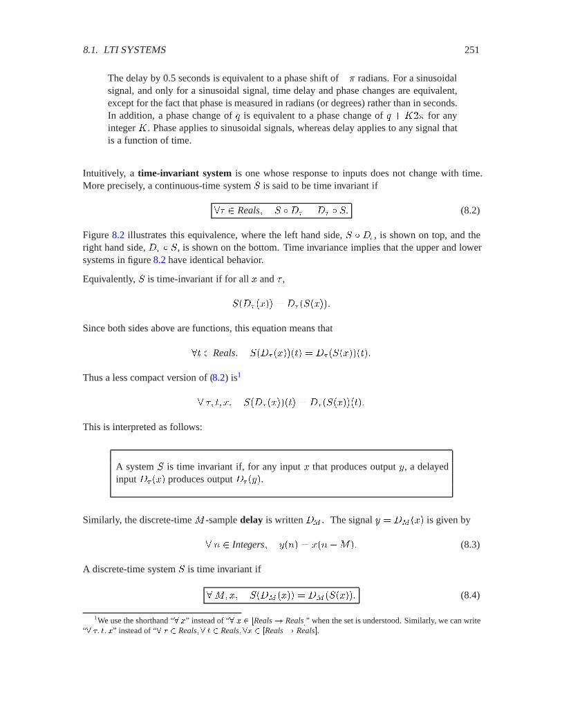
8.1. LTI SYSTEMS 251
The delay by 0.5 seconds is equivalent to a phase shift of �� radians. For a sinusoidalsignal, and only for a sinusoidal signal, time delay and phase changes are equivalent,except for the fact that phase is measured in radians (or degrees) rather than in seconds.In addition, a phase change of 8 is equivalent to a phase change of 8 � >�� for anyinteger > . Phase applies to sinusoidal signals, whereas delay applies to any signal thatis a function of time.
Intuitively, a time-invariant system is one whose response to inputs does not change with time.More precisely, a continuous-time system . is said to be time invariant if
�� Reals� . Æ�( � �( Æ .� (8.2)
Figure 8.2 illustrates this equivalence, where the left hand side, . Æ �( , is shown on top, and theright hand side, �( Æ ., is shown on the bottom. Time invariance implies that the upper and lowersystems in figure 8.2 have identical behavior.
Equivalently, . is time-invariant if for all � and � ,
.��( ���� � �( �.�����
Since both sides above are functions, this equation means that
� Reals� .��( ������ � �( �.�������
Thus a less compact version of (8.2) is1
� �� � �� .��( ������ � �( �.�������
This is interpreted as follows:
A system . is time invariant if, for any input � that produces output �, a delayedinput �( ��� produces output �( ���.
Similarly, the discrete-time 3 -sample delay is written �� . The signal � � �� ��� is given by
� � Integers� ���� � ����3�� (8.3)
A discrete-time system . is time invariant if
�3��� .��� ���� � �� �.����� (8.4)
1We use the shorthand “� �” instead of “� � � �Reals� Reals�” when the set is understood. Similarly, we can write“� �� �� �” instead of “� � � Reals� � � � Reals� �� � �Reals� Reals�.
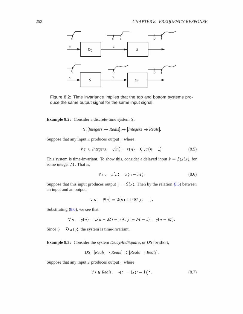
252 CHAPTER 8. FREQUENCY RESPONSE
xDτS
z
y
0 τ0
00
τ0
τ0
xDτ S
Figure 8.2: Time invariance implies that the top and bottom systems pro-duce the same output signal for the same input signal.
Example 8.2: Consider a discrete-time system .,
.� �Integers� Reals�� �Integers� Reals��
Suppose that any input � produces output � where
� � Integers� ���� � ���� � ������ �� (8.5)
This system is time-invariant. To show this, consider a delayed input �� � �� ���, forsome integer 3 . That is,
� �� ����� � ����3�� (8.6)
Suppose that this input produces output �� � .����. Then by the relation (8.5) betweenan input and an output,
� �� ����� � ����� � ������� ��
Substituting (8.6), we see that
� �� ����� � ����3� � ������3 � � � ����3��
Since �� � �� ���, the system is time-invariant.
Example 8.3: Consider the system DelayAndSquare, or DSfor short,
DS � �Reals� Reals�� �Reals� Reals��
Suppose that any input � produces output � where
� Reals� ��� � ���� ���� (8.7)

8.1. LTI SYSTEMS 253
This system is time-invariant. To show this, consider a delayed input �� � �( ���, forsome real number � . That is,
� � ���� � ��� ��� (8.8)
Suppose that this input produces output �� � .����. Then by the relation (8.7) betweenan input and an output,
� � ���� � ����� ����
Substituting (8.8), we see that
� � ���� � ���� � ���� � ��� ���
Since �� � �( ���, the system is time-invariant.
Example 8.4: Consider a system ReverseTimeor RT,
RT � �Reals� Reals�� �Reals� Reals��
where any input � produces output � related by
� Reals� ��� � ����� (8.9)
This system is not time-invariant. To show this, consider a delayed input �� � �( ���,for some real number � . That is,
� � ���� � ��� ��� (8.10)
Suppose that this input produces output �� � .����. Then by the relation (8.9) betweenan input and an output,
� � ���� � ������Substituting (8.10), we see that
� � ���� � ���� �� �� ��� �� � ���� ���
Since �� �� �( ���, the system is not time-invariant.
To be completely convinced that these two signals are different in general, consider aparticular signal � such that �� ��� � , and take � � . Then ���� � �, but��( ������ � .
Time invariance is a mathematical fiction. No electronic system is time invariant in the strict sense.For one thing, such a system is turned on at some point in time. Clearly, its behavior before it isturned on is not the same as its behavior after it is turned on. Nevertheless, it proves to be a veryconvenient mathematical fiction, and it is a reasonable approximation for many systems if theirbehavior is constant over a relatively long period of time (relative to whatever phenomenon we arestudying). For example, your audio amplifier is not a time-invariant system. Its behavior changesdrastically when you turn it on or off, and changes less drastically when you raise or lower the

254 CHAPTER 8. FREQUENCY RESPONSE
volume. However, for the duration of a compact disc, if you leave the volume fixed, the system canbe reasonably approximated as being time-invariant.
Some systems have a similar property even though they operate on signals whose domain is nottime. For example, the domain of an image is a region of a plane. The output of an image process-ing system may not depend significantly on where in the plane the input image is placed. Shiftingthe input image will only shift the output image by the same amount. This property which general-izes time invariance and holds for some image processing systems, is called shift invariance (seeproblem 5).
8.1.2 Linearity
Consider the set of signals whose range is Realsor Complex. Such signals are real-valued functionsor complex-valued functions. Since real-valued functions are a subset of complex-valued functions,we only need to talk about complex-valued functions. It does not matter (for now) whether they arecontinuous-time signals or discrete-time signals. The domain could be Realsor Integers.
Suppose � is a complex-valued function and � is a complex constant. Then we can define a newcomplex-valued function �� such that for all in the domain of �,
������ � �������
In other words, the new function, which we call ��, is simply scaled by the constant �.
Similarly, given two complex-valued functions �� and �� with the same domain and range, we candefine a new function ��� � ��� such that for all in the domain,
��� � ����� � ���� � �����
Consider the set of all systems that map complex-valued functions to complex-valued functions.Such systems are called complex systems. Again, it does not matter (for now) whether they arediscrete-time systems or continuous-time systems. Suppose that . is a complex system. . is saidto be linear if for all � Complexand for all complex signals �,
.���� � �.��� (8.11)
and for all complex signals �� and �� in the domain of .,
.��� � ��� � .���� � .���� (8.12)
The first of these—called the homogeneity property—says that if you scale the input, the outputis scaled. The second one—called the additivity property—says that if the input is described asthe sum of two component signals, then the output can be described as the sum of two signals thatwould result from the components alone. Recall that linear functions were introduced in section5.2. A linear system is one whose function relating the output to the input is linear.
In pictures, the first property says that the two systems in figure 8.3 are equivalent if . is linear.Here, the triangle represents the scaling operation. The second property says that the two systemsin figure 8.4 are equivalent.
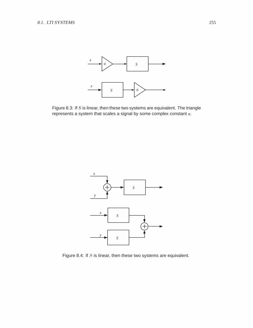
8.1. LTI SYSTEMS 255
Sax
S ax
Figure 8.3: If . is linear, then these two systems are equivalent. The trianglerepresents a system that scales a signal by some complex constant �.
S
x
y
S
S
x
y
Figure 8.4: If . is linear, then these two systems are equivalent.
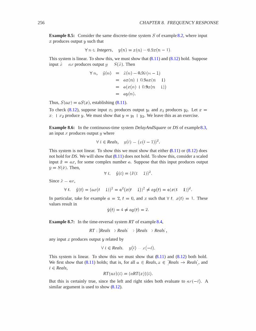
256 CHAPTER 8. FREQUENCY RESPONSE
Example 8.5: Consider the same discrete-time system . of example 8.2, where input� produces output � such that
� � Integers� ���� � ���� � ������ ��
This system is linear. To show this, we must show that (8.11) and (8.12) hold. Supposeinput �� � �� produces output �� � .����. Then
� �� ����� � ����� � ������� �
� ����� � ������ � �
� ������ � ������ ��
� ������
Thus, .���� � �.���, establishing (8.11).
To check (8.12), suppose input �� produces output �� and �� produces ��. Let � ��� � �� produce �. We must show that � � �� � ��. We leave this as an exercise.
Example 8.6: In the continuous-time system DelayAndSquareor DSof example8.3,an input � produces output � where
� Reals� ��� � ���� ����
This system is not linear. To show this we must show that either (8.11) or (8.12) doesnot hold for DS. We will show that (8.11) does not hold. To show this, consider a scaledinput �� � ��, for some complex number �. Suppose that this input produces output�� � .����. Then,
� � ���� � ����� ����
Since �� � ��,
� � ���� � ����� ��� � ������ ��� �� ���� � ����� ����
In particular, take for example � � �, � , and � such that � � ��� � . Thesevalues result in
���� � � �� ���� � ��
Example 8.7: In the time-reversal system RT of example 8.4,
RT � �Reals� Reals�� �Reals� Reals��
any input � produces output � related by
� Reals� ��� � �����This system is linear. To show this we must show that (8.11) and (8.12) both hold.We first show that (8.11) holds; that is, for all � Reals� � �Reals� Reals�, and Reals,
RT������ � ��RT�������
But this is certainly true, since the left and right sides both evaluate to �����. Asimilar argument is used to show (8.12).
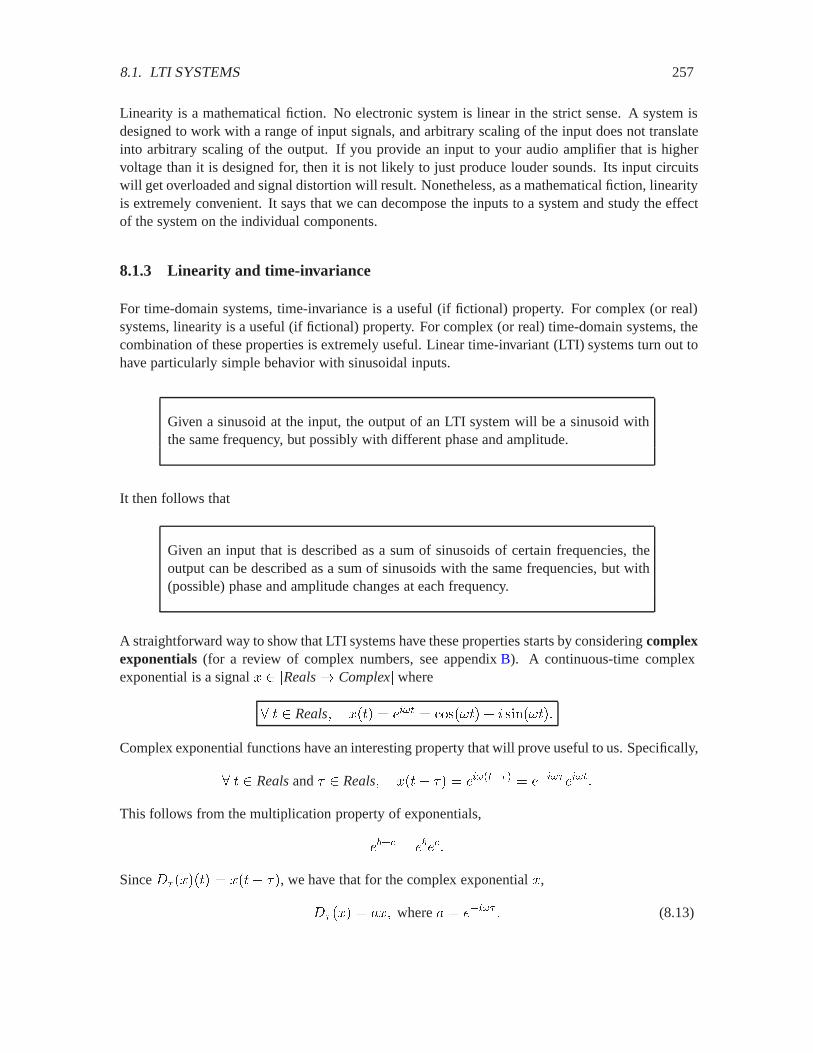
8.1. LTI SYSTEMS 257
Linearity is a mathematical fiction. No electronic system is linear in the strict sense. A system isdesigned to work with a range of input signals, and arbitrary scaling of the input does not translateinto arbitrary scaling of the output. If you provide an input to your audio amplifier that is highervoltage than it is designed for, then it is not likely to just produce louder sounds. Its input circuitswill get overloaded and signal distortion will result. Nonetheless, as a mathematical fiction, linearityis extremely convenient. It says that we can decompose the inputs to a system and study the effectof the system on the individual components.
8.1.3 Linearity and time-invariance
For time-domain systems, time-invariance is a useful (if fictional) property. For complex (or real)systems, linearity is a useful (if fictional) property. For complex (or real) time-domain systems, thecombination of these properties is extremely useful. Linear time-invariant (LTI) systems turn out tohave particularly simple behavior with sinusoidal inputs.
Given a sinusoid at the input, the output of an LTI system will be a sinusoid withthe same frequency, but possibly with different phase and amplitude.
It then follows that
Given an input that is described as a sum of sinusoids of certain frequencies, theoutput can be described as a sum of sinusoids with the same frequencies, but with(possible) phase and amplitude changes at each frequency.
A straightforward way to show that LTI systems have these properties starts by considering complexexponentials (for a review of complex numbers, see appendix B). A continuous-time complexexponential is a signal � �Reals� Complex� where
� Reals� ��� � ���� � ������ � & �������
Complex exponential functions have an interesting property that will prove useful to us. Specifically,
� Realsand � Reals� ��� �� � ��� ��(� � ����( �����
This follows from the multiplication property of exponentials,
���� � �����
Since �( ����� � ��� ��, we have that for the complex exponential �,
�( ��� � ��� where � � ����( � (8.13)
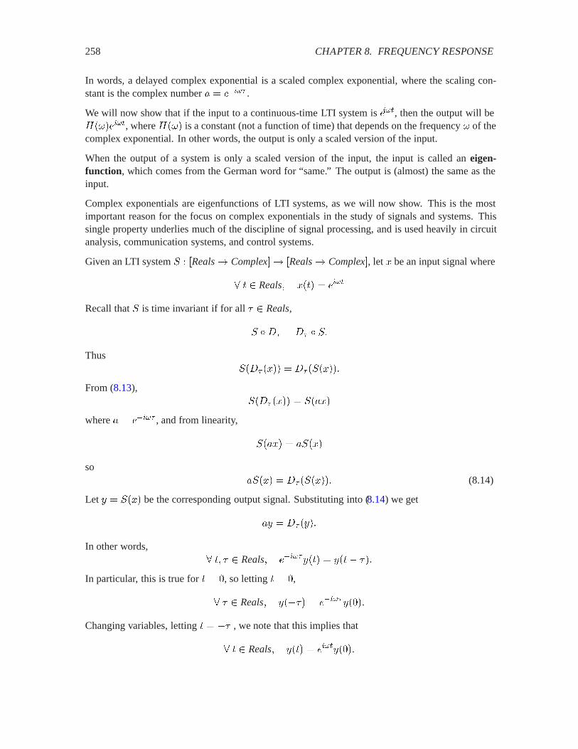
258 CHAPTER 8. FREQUENCY RESPONSE
In words, a delayed complex exponential is a scaled complex exponential, where the scaling con-stant is the complex number � � ����( .
We will now show that if the input to a continuous-time LTI system is ����, then the output will be;�������, where ;��� is a constant (not a function of time) that depends on the frequency � of thecomplex exponential. In other words, the output is only a scaled version of the input.
When the output of a system is only a scaled version of the input, the input is called an eigen-function, which comes from the German word for “same.” The output is (almost) the same as theinput.
Complex exponentials are eigenfunctions of LTI systems, as we will now show. This is the mostimportant reason for the focus on complex exponentials in the study of signals and systems. Thissingle property underlies much of the discipline of signal processing, and is used heavily in circuitanalysis, communication systems, and control systems.
Given an LTI system . � �Reals� Complex�� �Reals� Complex�, let � be an input signal where
� Reals� ��� � ����
Recall that . is time invariant if for all � Reals,
. Æ�( � �( Æ .�
Thus.��( ���� � �( �.�����
From (8.13),.��( ���� � .����
where � � ����( , and from linearity,
.���� � �.���
so�.��� � �( �.����� (8.14)
Let � � .��� be the corresponding output signal. Substituting into (8.14) we get
�� � �( ����
In other words,� � � Reals� ����(��� � ��� ���
In particular, this is true for � , so letting � ,
� � Reals� ����� � ����(����
Changing variables, letting � �� , we note that this implies that
� Reals� ��� � ��������
8.2. FINDING AND USING THE FREQUENCY RESPONSE 259
Recall that ��� is the output evaluated at 0 when the input is ����. It is a constant, in that it does notdepend on , so this establishes that the output is a complex exponential, just like the input, exceptthat it is scaled by ���. However, ��� does, in general, depend on �, so we define the function;�Reals� Complexby
� � Reals� ;��� � ��� � �.������� where � Reals� ��� � ����. (8.15)
That is, ;��� is the output at time zero when the input is a complex exponential with frequency �.
Using this notation, we write the output � as
� Reals� ��� � ;�������
when the input is ����. Note that ;��� is a function of � Reals, the frequency of the inputcomplex exponential.
The function ; � Reals� Complexis called the frequency response. It defines the response ofthe LTI system to a complex exponential input at any given frequency. It gives the scaling factorthat the system imposes on that complex exponential.
For discrete-time systems, the situation is similar. By reasoning identical to that above, for an LTIsystem, if the input is a discrete complex exponential,
� � Integers� ���� � ����
then the output is the same complex exponential scaled by a constant (a complex number that doesnot depend on time),
� � Integers� ���� � ;�������
; is once again called the frequency response, and since it is a function of �, and is possiblycomplex valued, it has the form ;�Reals� Complex.
There is one key difference, however, between discrete-time systems and continuous-time systems.Since � is an integer, notice that
���� � �� ���)�� � �� ��)���
and so on. That is, a discrete complex exponential with frequency � is identical to a discrete complexexponential with frequency � � �>�, for any integer > . The frequency response, therefore, mustbe identical at these frequencies, since the inputs are identical. That is
�� Reals� ;��� � ;�� � �>��
for any integer > . That is, a discrete-time frequency response is periodic with period ��.
8.2 Finding and using the frequency response
We have seen that if the input to an LTI system is a complex exponential signal � �Reals�Complex� where
� Reals� ��� � ���� � ������ � & �������
260 CHAPTER 8. FREQUENCY RESPONSE
then the output is
� Reals� ��� � ;�������� (8.16)
where ;��� is a (possibly complex-valued) number that is a property of the system. ;��� is calledthe frequency response at frequency �.
Example 8.8: Consider a delay system . � �� , for some Reals. It is anLTI system, as is easy to verify by checking that (8.2), (8.11), and (8.12) are satisfied.Suppose the input to the delay system is the complex exponential � given by
� Reals� ��� � �����
Then the output � satisfies
� Reals� ��� � ��� ��� � � ����� �����
Comparing this to (8.16) we see that the frequency response of the delay is
;��� � ����� �
Example 8.9: Consider a discrete-time 3 -sample delay system . � �� . If � �.��� then � is given by
� � Integers� ���� � ����3�� (8.17)
This is an LTI system, as is easy to verify. We could find the frequency response exactlythe same way as in the previous example, but instead we use a slightly different method.Since the system is LTI, we know that if the input is � such that for all � Integers,���� � ����, then the output is ;�������, where ; is the frequency response. Byplugging this input and output into (8.17), we get
;������� � ��� ���� � ��������� �
Divide both sides by ���� to get
;��� � ����� �
The techniques in the previous examples can be used to find the frequency response of more compli-cated systems. Simply replace the input � in a difference equation like (8.17) with ����, and replacethe output � with ;�������, and then solve for ;���.
Example 8.10: Consider a discrete-time, length two moving average, given by thedifference equation
� � Integers� ���� � ����� � ���� �����
where � is the input and � is the output. When the input for all � is ����, this becomes
;������� � ����� � ��� ��������
Solving for ;���, we find that the frequency response is
;��� � � � ��������

8.2. FINDING AND USING THE FREQUENCY RESPONSE 261
R
Cx(t) y(t)+
-
+
-
Figure 8.5: The RC circuit of example 8.11.
A similar approach can find the frequency response of a continuous-time system described by adifferential equation.
Example 8.11: Consider a continuous-time system with input � and output � relatedby the differential equation
� Reals� ����
��� � ��� � ���� (8.18)
where � and � are real-valued constants. This differential equation describes the RCcircuit of figure 8.5, which consists of an �-ohm resistance in series with a �-faradcapacitor. The circuit has input voltage �, provided by a voltage source, shown as acircle on the left. The output is the voltage � across the capacitor. Kirchhoff’s voltagelaw gives the differential equation. It is easy to verify that this differntial equationdescribes an LTI system.
We can determine the frequency response of this system by assuming that the input �is given by � Reals, ��� � ����, and finding the output. Since the system is LTI,the output will be given by ��� � ;�������. Plugging these values for � and � into(8.18) gives
���&��;������� �;������� � ����� (8.19)
because��
��� � &�;��������
Dividing both sides of (8.19) by ���� yields the frequency response of this circuit,
�� Reals� ;��� �
� &����
8.2.1 Linear difference and differential equations
The procedure of example 8.10 can be used to write down by inspection the frequency response ofany high-order linear difference equation of the form, � � Integers,
������ � ������ � � � �������� � ������ � ������ � � � ������3�� (8.20)
262 CHAPTER 8. FREQUENCY RESPONSE
The coefficients of this difference equation, ��� � �� and ��� � �� � are real constants. (Theycould also be complex.) This describes an LTI system, and a good way to recognize that a discrete-time system is LTI is to write it in this form. If the input for all � is ���� � ����, then the outputfor all � is ���� � ;�������. Plugging these values of input and output into (8.20) gives,
��;������� � ��;������ ���� � � ��;������ ����
� ������ � ���
�� ���� � � ����� �����
Recognizing that ��� ���� � ���������, we can divide both sides by ���� and solve for ;��� toget
�� Reals� ;��� � ����� ��������� ���
����� ��������� ���(8.21)
Observe that the frequency response (8.21) is a ratio of two polynomials in ���� .
Example 8.12: Consider an LTI system given by the difference equation
�� Integers� ����� ���� �� � ���� � ����� � � ���� ���
Its frequency response is
�� Reals� ;��� � � ����� � �����
� ������
In a similar way one can obtain the frequency response of any linear differential equation of theform,
� Reals� �����
����� �����
��������� � ��
���
����� ��� ��
���������� (8.22)
where the coefficients �� � � �� and �� � � ��� are real (or complex) constants. This describesan LTI system, and a good way to recognize that a continuous-time system is LTI is to write it inthis form. If the input for all is ��� � ����, the output for all is ��� � ;�������. Pluggingthese values of input and output into (8.22), and recognizing that
��
������ � �&��������
gives,
�� �&���;������� � � ���&��;������� � ��;������� �
�� �&������� � � ���&������ � ���
����
We can divide both sides by ���� to get
�� Reals� ;��� � �� ����������� �������� ����������� ������
(8.23)
Observe that the frequency response (8.23) is a ratio of two polynomials in &�.
8.2. FINDING AND USING THE FREQUENCY RESPONSE 263
Basics: Sinusoids in terms of complex exponentials
Euler’s formula states that
��* � ����#� � & ����#��
The complex conjugate is
���* � ����#�� & ����#��
Summing these,��* � ���* � �!4��#�
or����#� � ���* � ���*����
Thus, for example,������ � ����� � ���������
Similarly,
����#� � �&���* � ���*����
In appendix A we show that many useful trigonometric identities are easily derivedfrom these simple relations.
Example 8.13: Consider the continuous-time system given by the differential equation
� Reals����
����� �
��
��� � ���� �
��
�� ����
where � is the input and � is the output. It has frequency response
�� Reals� ;��� �&� �
�&��� � �&� � ��
Complex exponentials as inputs are rather abstract. We have seen that with audio signals, sinusoidalsignals are intrinsically significant because the human ear interprets the frequency of the sinusoidas its tone. Note that a real-valued sinusoidal signal can be given as a combination of exponentialsignals (see box on page 263),
������ � ����� � ���������
Thus, if this is the input to an LTI system with frequency response ; , then the output will be
��� � �;������� �;������������� (8.25)
Many (or most) LTI systems are not capable of producing complex-valued outputs when the inputis real, so for such systems, this ��� must be real. This implies that
;��� � ;������ (8.26)

264 CHAPTER 8. FREQUENCY RESPONSE
Tips and Tricks: Phasors
Consider a general continuous-time sinusoidal signal,
� Reals� ��� � � ������ <��
Here � is the amplitude, < is the phase, and � is the frequency of the sinewave.(We call this a sinewave, even though we are using cosine to describe it.) The unitsof < are radians. The units of � are radians per second, assuming is in seconds.This can be written
��� � Re���� ���+� � Re����+���� � Re������
where � � ���+ is called the complex amplitude or phasor. The representation
��� � Re������ (8.24)
is called the phasor representation of �. It can be convenient.
Example 8.14: Consider summing two sinusoids with the same fre-quency,
��� � �� ������ <�� ��� ������ <���
This is particularly easy using phasors, since
��� � Re���� ��������
� ��� ���� ������ � ��� �����
where �� � ����+� and �� � ���
�+� . Thus, addition of the sinusoidsreduces to addition of two complex numbers.
The exponential ����� in (8.24) is complex valued. If we represent it in a two-dimensional plane as in figure 8.6, it will rotate in a counter-clockwise direction as increases. The frequency of rotation will be � radians per second. At time 0 itwill be � , shown in gray. The real-valued sinewave ��� is the projection of �����
on the real axis, namely
Re������ � ��� ������ � ���
The sum of two sinusoids with the same frequency is similarly depicted in figure8.7. The two phasors, �� and �� are put head to tail and then rotated together. Asimilar method can be used to add sinusoids of different frequencies, but then thetwo vectors will rotate at different rates.
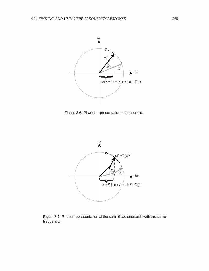
8.2. FINDING AND USING THE FREQUENCY RESPONSE 265
Re
ImX
Xeiωt
ωt
{Re{Xeiωt} = |X| cos(ωt + ∠X)
Figure 8.6: Phasor representation of a sinusoid.
Re
Im
X1
(X1+X2)eiωt
{|X1+X2| cos(ωt + ∠(X1+X2))
X2
Figure 8.7: Phasor representation of the sum of two sinusoids with the samefrequency.
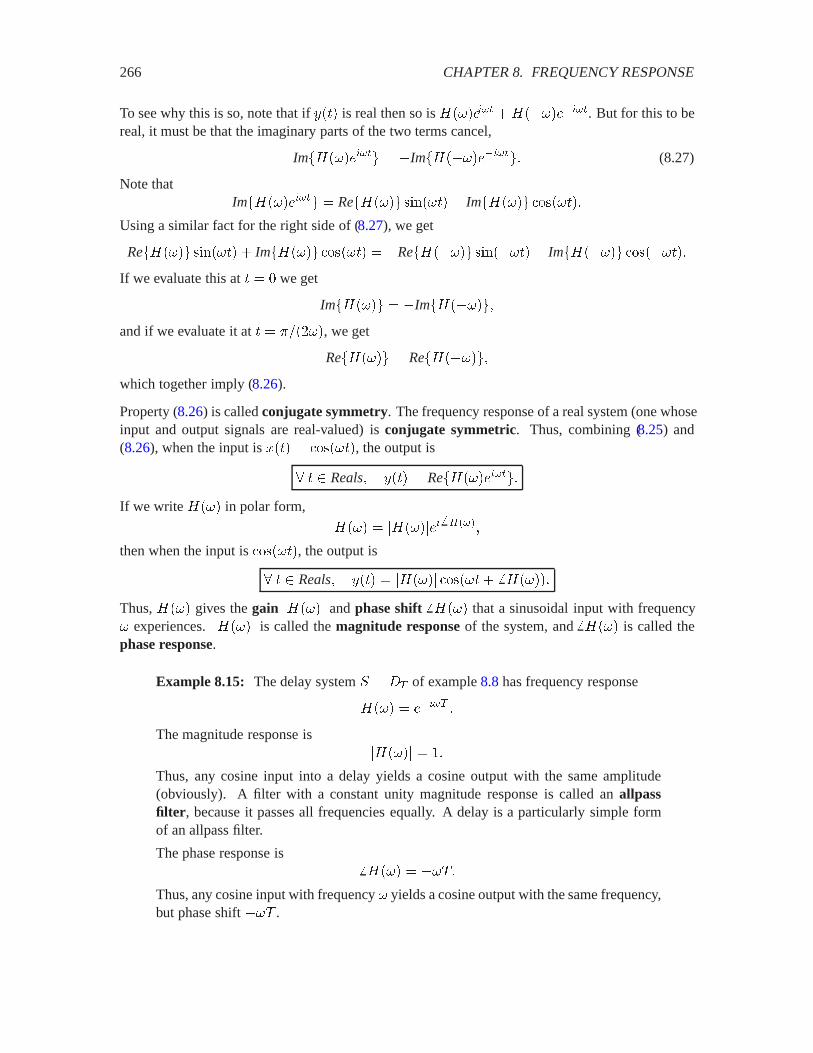
266 CHAPTER 8. FREQUENCY RESPONSE
To see why this is so, note that if ��� is real then so is ;������� �;���������. But for this to bereal, it must be that the imaginary parts of the two terms cancel,
Im�;������� � �Im�;���������� (8.27)
Note thatIm�;������� � Re�;��� ������ � Im�;��� �������
Using a similar fact for the right side of (8.27), we get
Re�;��� ������ � Im�;��� ������ � �Re�;���� �������� Im�;���� ��������If we evaluate this at � we get
Im�;��� � �Im�;�����and if we evaluate it at � ������, we get
Re�;��� � Re�;�����which together imply (8.26).
Property (8.26) is called conjugate symmetry. The frequency response of a real system (one whoseinput and output signals are real-valued) is conjugate symmetric. Thus, combining (8.25) and(8.26), when the input is ��� � ������, the output is
� Reals� ��� � Re�;��������If we write ;��� in polar form,
;��� � �;������� & ���
then when the input is ������, the output is
� Reals� ��� � �;���� ������ � ;�����
Thus, ;��� gives the gain �;���� and phase shift � ;��� that a sinusoidal input with frequency� experiences. �;���� is called the magnitude response of the system, and � ;��� is called thephase response.
Example 8.15: The delay system . � �� of example 8.8 has frequency response
;��� � ����� �
The magnitude response is�;���� � �
Thus, any cosine input into a delay yields a cosine output with the same amplitude(obviously). A filter with a constant unity magnitude response is called an allpassfilter, because it passes all frequencies equally. A delay is a particularly simple formof an allpass filter.
The phase response is� ;��� � ���
Thus, any cosine input with frequency � yields a cosine output with the same frequency,but phase shift �� .
8.2. FINDING AND USING THE FREQUENCY RESPONSE 267
Example 8.16: The 3 -sample discrete-time delay of example 8.9 is also an allpassfilter. Its phase response is
� ;��� � ��3�
Example 8.17: The magnitude response of the length-two moving average consideredin example 8.10 is
�;���� � �� � ���������We can plot this using the following Matlab code, which (after adjusting the labels)results in figure 8.2.1.
omega = [0:pi/250:pi];H = (1 + exp(-i*omega))/2;plot(omega, abs(H));
Notice that at frequency zero (a cosine with zero frequency has constant value), themagnitude response is 1. That is, a constant signal gets through the filter without anyreduction in amplitude. This is expected, since the average of two neighboring samplesof a constant signal is simply the value of the constant signal. Notice that the mag-nitude response decreases as the frequency increases. Thus, higher frequency signalshave their amplitudes reduced more by the filter than lower frequency signals. Sucha filter is called a lowpass filter because it passes lower frequencies better than higherfrequencies.
Example 8.18: The RC circuit of example 8.11 has frequency response given by
�� Reals� ;��� �
� &����
We can express this in polar form, ;��� � �;������� & �� to get the magnitude andphase responses,
�;���� � ! � ������
� � ;��� � � ���������
If for all , ��� � ������, then ��� � �;���� ������ � ;����. Since �;���� � as � ��, this RC circuit is a (not very good) low-pass filter.
Often, we are given a frequency response, rather than some other description of an LTI system suchas a difference equation. The frequency response, in fact, tells us everything we need to know aboutthe system. The next example begins the exploration of that idea.
Example 8.19: Suppose that the frequency response ; of a discrete-time LTI systemFilter is given by
� � Reals� ;��� � �������

268 CHAPTER 8. FREQUENCY RESPONSE
0 0.5 1 1.5 2 2.5 30
0.1
0.2
0.3
0.4
0.5
0.6
0.7
0.8
0.9
1
frequency in radians/sample
Figure 8.8: The magnitude response of a length-two moving average.
where � has units of radians/sample. Suppose that the input signal �� Integers� Realsis such that for all � Integers,
���� �
�� � even� � odd
We can determine the output. All we have to do is notice that the input can be writtenas
���� � ��������
Thus, the input is a cosine with frequency � radians/sample. Hence, the output is
���� � �;���� ������� � ;���� � ������� � �����
This input is passed unchanged by the system.
Suppose instead that the input is given by
���� � ��
Once again, the input is a cosine, but this time with zero frequency,
���� � � �������
Hence the output is
���� � �;��� � ������ � ;��� � � � �����

8.2. FINDING AND USING THE FREQUENCY RESPONSE 269
This input is also passed unchanged by the system.
Suppose instead that the input is
���� � ����������
This input is given explicitly as a cosine, making our task easier. The output is
���� � �;������ �������� � � ;������
� �������� � ��
� � ���������
� ������
This input is inverted by the system.
Finally, suppose that the input is
���� � ����������
The output is���� � �;������ �������� � � ;������ � �
This input is filtered out by the system.
8.2.2 The Fourier series with complex exponentials
The Fourier series for a continuous-time, periodic signal � � Reals� Realswith period ( � �����,can be written as (see (7.4))
��� � �� ������
�� ����6��� <���
For reasons that we can now understand, the Fourier series is usually written in terms of complexexponentials rather than cosines. Since complex exponentials are eigenfunctions of LTI systems,this form of the Fourier series decomposes a signal into components that when processed by thesystem are only scaled.
Each term of the Fourier series expansion has the form
�� ����6��� <��
which we can write (see box on page 263)
�� ����6��� <�� � ����� �����+�� � ��� �����+������
So the Fourier series can also be written
��� � �� ������
��
���� �����+�� � ��� �����+����
270 CHAPTER 8. FREQUENCY RESPONSE
Observe that
�� �����+�� � ��������+� �
and let
�� �
����
�� if 6 � �����
�+� if 6 2 ������
��+� if 6 ) (8.28)
Then the Fourier series becomes
��� ���
�������
������ (8.29)
This is the form in which one usually sees the Fourier series. Notice from (8.28) that the Fourierseries coefficients are conjugate symmetric,
�� � �����
Of course, since (8.29) is an infinite sum, we need to worry about convergence (see box on page234).
The discrete-time Fourier series (DFS) can be similarly written. If � � Integers� Realsis aperiodic signal with period ( � �����, then we can write
���� �#������
�������� (8.30)
for suitably defined coefficients ��. Relating the coefficients �� to the coefficients �� and <� is abit more difficult in the discrete-time case than in the continuous-time case (see box on page271).
There are two differences between (8.29) and (8.30). First, the sum in the discrete-time case isfinite, making it manageable by computer. Second, it is exact for any periodic waveform. There areno mathematically tricky cases, and no approximation needed.
8.2.3 Examples
The Fourier series coefficients �� of a square wave are shown in figure 7.6 in the previous chapter.The magnitudes of the corresponding coefficients �� for the Fourier series expansion of (8.29) areshown in figure 8.9. Since each cosine is composed of two complex exponentials, there are twice asmany coefficients.
Notice the symmetry in the figure. There are frequency components shown at both positive andnegative frequencies. Notice also that the amplitude of the components is half that in figure7.6,���� � ������. This is because there are now two components, one at negative frequencies and oneat positive frequencies, that contribute.
8.2. FINDING AND USING THE FREQUENCY RESPONSE 271
Probing further: Relating DFS coefficients
We have two discrete-time Fourier series expansions (see (8.30) and (7.8)),
���� �#������
�������� (8.31)
���� � �� ������
�� ����6���� <��� > �
��(� ��� if ( is odd(�� if ( is even
There is a relationship between the coefficients ��, <� and ��, but the relationshipis more complicated than in the continuous-time case, given by (8.28). To developthat relationship, begin with the second of these expansions and write
���� � �� ������
��
���� �����+�� � ��� �����+����
Note that since �� � ���(, then for all integers �, ����#� � , so
��� �����+�� � ��� �����+������#� � �� �� #�����+���
Thus,
���� � �� ������
��
���+�������� �
�����
��
����+����� #����
� �� ������
��
���+�������� �
#������
�#��
����+��������
by change of variables. Comparing this against (8.31),
�� �
��������
�� if 6 � ���
�+��� if 6 �� �> � ���
�+��� ������+��� � �� ����<�� if 6 � >
�#�����+��� if 6 �> � � � (�
This relationship is more complicated than (8.28). Fortunately, it is rare that weneed to use both forms of the DFS, so we can usually just pick one of the twoforms and work only with its set of coefficients.
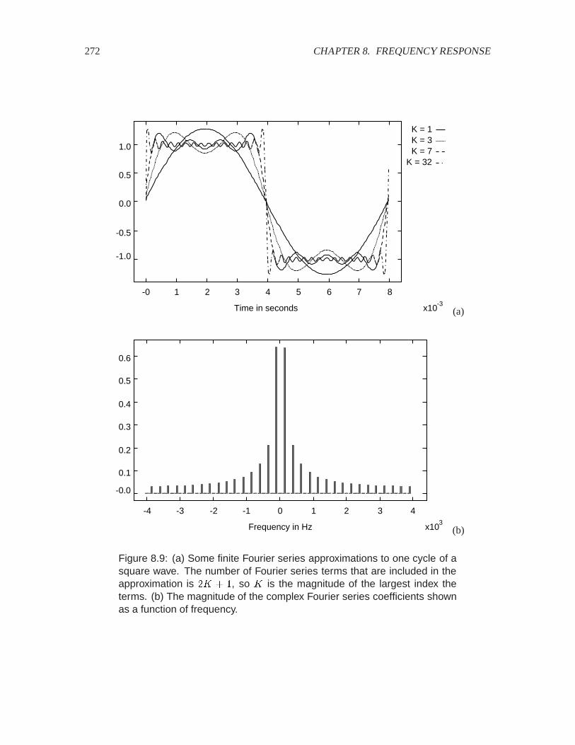
272 CHAPTER 8. FREQUENCY RESPONSE
-3x10
K = 1K = 3K = 7
K = 32
-1.0
-0.5
0.0
0.5
1.0
-0 1 2 3 4 5 6 7 8
Time in seconds (a)
3x10
-0.0
0.1
0.2
0.3
0.4
0.5
0.6
-4 -3 -2 -1 0 1 2 3 4
Frequency in Hz (b)
Figure 8.9: (a) Some finite Fourier series approximations to one cycle of asquare wave. The number of Fourier series terms that are included in theapproximation is �> � , so > is the magnitude of the largest index theterms. (b) The magnitude of the complex Fourier series coefficients shownas a function of frequency.
8.3. DETERMINING THE FOURIER SERIES COEFFICIENTS 273
8.3 Determining the Fourier series coefficients
We have seen in the previous chapter that determining the Fourier series coefficients by directlyattempting to determine the amplitude of individual frequency components can be difficult, evenwhen the individual frequency components are known. Usually, however, they are not known. Ageneral formula for computing the coefficients for a continuous-time periodic signal is
�� � �#
#"������������� (8.32)
The '-th Fourier series coefficient is obtained by multiplying � by a complex exponential withfrequency �'�� and averaging. The validity of this equation is demonstrated in the box on page274.
The discrete-time case is somewhat simpler. A discrete-time periodic signal � with period ( Integershas Fourier series coefficients given by
�� � �#
#������
��'�������� � (8.33)
This can be shown by manipulations similar to those in the box on page274. The practical impor-tance in computing is much greater than that of the Fourier series for continuous-time signals. Sincethis sum is finite, the DFS coefficients can be easily computed precisely on a computer.
8.3.1 Negative frequencies
The Fourier series expansion for a periodic signal ��� is
��� ���
����
��������
This includes Fourier series coefficients for the constant term (when 6 � , ������ � �, plus thefundamental and harmonics �6 � �. But it also includes terms that seem to correspond to negativefrequencies. When 6 � �, the frequency 6�� is negative. These negative frequencies balance thepositive ones so that the resulting sum is real-valued.
8.4 Frequency response and the Fourier series
Recall that if the input to an LTI system . is a complex exponential signal � �Reals� Complex�where
� Reals� ��� � ����� � ������� � & ��������

274 CHAPTER 8. FREQUENCY RESPONSE
Probing further: Formula for Fourier series coefficients
To see that (8.32) is valid, try substituting for ��� its Fourier series expansion,
��� ���
����
��������
to get
�� �
(
� #
�
������
�����������������
Exchange the integral and summation (assuming this is valid, see box on page275)to get
�� �
(
������
��
� #
����������������
The exponentials can be combined to get
�� �
(
������
��
� #
��� ���������
In the summation, where 6 varies over all integers, there will be exactly one termof the summation where 6 � '. In that term, the integral evaluates to (. For therest of the terms, 6 �� '. Separating these two situations, we can write
�� � �� �
(
�������� ���
��
#��
�� ���������
where the first term �� is the value of the term in the summation where 6 � '.For each remaining term of the summation, the integral evaluates to zero, thusestablishing our result. To show that the integral evaluates to zero, let � � 6 �',and note that � �� . Then� #
�������� �
� #
����������� &
� #
����������
Since �� � ���(, these two integrals exactly span one or more complete cycles ofthe cosine or sine, and hence integrate to zero.
8.4. FREQUENCY RESPONSE AND THE FOURIER SERIES 275
Probing further: Exchanging integrals and summations
The demonstration of the validity of the formula for the Fourier series coefficientsin the box on page 274 relies on being able to exchange an integral and an infi-nite summation. The infinite summation can be given as a limit of a sequence offunctions
�� �� ���
����
���������
Thus, we wish to exchange the integral and limit in
�� �
(
� #
�� !����
�� �����
A sufficient condition for being able to perform the exchange is that the limit con-verges uniformly in the interval [0, p]. A sufficient condition for uniform conver-gence is that � is continuous and that its first derivative is piecewise continuous.
See R. G. Bartle, The Elements of Real Analysis, Second Edition, John Wiley &Sons, 1976, p. 241.
then the output for all is��� � ;�����
�����
where the complex number ;���� is the frequency response of the system at the fundamentalfrequency �� of the periodic input. It is equal to the output at time zero ��� when the input is �����.; itself is a function ;�Reals� Complexthat in principle can be evaluated for any frequency� Reals, including negative frequencies.
Recall further that if an input � to the system . is a periodic signal with period (, then it can berepresented as a Fourier series,
� Reals� ��� ���
����
���������
where �� � ���(. By linearity and time invariance of ., the output � � .��� for this periodicinput �, is given by
� Reals� ��� ���
����;�6������
������
Thus, linearity tells us that if the input is decomposed into a sum of components, then the outputcan be decomposed into a sum of components where each component is the response of the systemto a single input component. Linearity together with time invariance tells us that each component,which is a complex exponential, is simply scaled. Thus, the output is given by a Fourier series withcoefficients ��;�6���.
This major result is summarized below:

276 CHAPTER 8. FREQUENCY RESPONSE
S1 S2
S
x y z
Figure 8.10: The cascade connection of the two LTI systems is the system. � .� Æ.�. The frequency response is related by ���;��� � ;����;����.
For an LTI system, if the input is given by a sum of complex exponentials, then theoutput can be given by a sum of the same complex exponentials, each one scaledby the frequency response evaluated at the corresponding frequency.
Among other things, this result tells us:
� There are no frequency components in the output that were not in the input. The outputconsists of the same frequency components as the input, but with each component individuallyscaled.
� LTI systems can be used to enhance or suppress certain frequency components. Such opera-tions are called filtering.
� The frequency response function characterizes which frequencies are enhanced or suppressed,and also what phase shifts might be imposed on individual components by the system.
We will see many examples of filtering in the next chapter.
8.5 Frequency response of composite systems
In section 2.1.5 we studied several ways of composing systems (using block diagrams) to obtainmore complex, composite systems. We will see in this section that when each block is an LTIsystem, the resulting composite system is also LTI. Moreover, we can easily obtain the frequencyresponse of the composite system from the frequency response of each block. This provides auseful way to construct interesting and complex systems by assembling simpler components. Thistool works equally well with discrete and continuous systems.
8.5.1 Cascade connection
Consider the composite system . obtained by the cascade connection of systems .� and .� infigure 8.10. Suppose .� and .� are LTI. We first show that . � .� Æ .� is LTI. To show that . is

8.5. FREQUENCY RESPONSE OF COMPOSITE SYSTEMS 277
time-invariant, we must show that for any � , . Æ�( � �( Æ .. But,
. Æ�( � .� Æ .� Æ�(
� .� Æ�( Æ .�� since .� is time-invariant
� �( Æ .� Æ .�� since .� is time-invariant
� �( Æ .�
as required.
We now show that . is linear. Let � be any input signal and � any complex number. Then
.���� � �.� Æ .������� .��.������
� .���.������ since .� is linear
� �9�.������ since .� is linear
� �.����
Lastly, if � and � are two input signals, then
.��� �� � �.� Æ .����� ��
� .��.���� ���
� .��.���� � .������ since .� is linear
� .��.����� � .��.������ since .� is linear
� .��� � .����
This shows that . is linear.
We now compute the frequency response of .. Let ;�����;�����;��� be the frequency responseof .�, .�, and ., respectively, at the frequency �. Consider the complex exponential input � givenby
� Reals� ��� � �����
Then the signal � � .���� is a multiple of �, namely, � � ;�����. In particular, � is a (scaled)complex exponential, and so � � .���� is given by
� � ;����� � ;����;������
But since ;��� is the frequency response of . at the frequency �, we also have
� � .��� � ;�����
and so we obtain�� Reals� ;��� � ;����;����� (8.34)
The frequency response of the cascade composition is the product of the frequency responses ofthe components. Exactly the same formula applies in the discrete-time case. This is a remarkable
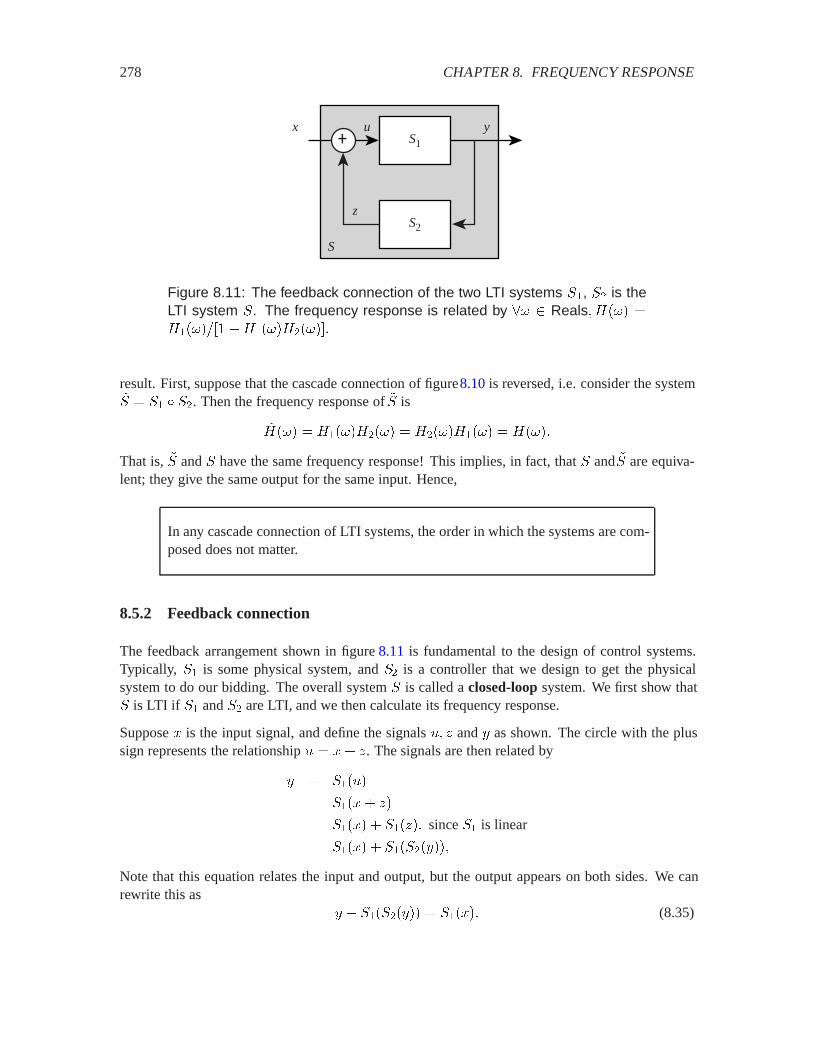
278 CHAPTER 8. FREQUENCY RESPONSE
S1
S2
S
x y+
z
u
Figure 8.11: The feedback connection of the two LTI systems .�, .� is theLTI system .. The frequency response is related by �� Reals�;��� �;������ �;����;�����.
result. First, suppose that the cascade connection of figure8.10 is reversed, i.e. consider the system". � .� Æ .�. Then the frequency response of ". is
";��� � ;����;���� � ;����;���� � ;����
That is, ". and . have the same frequency response! This implies, in fact, that . and ". are equiva-lent; they give the same output for the same input. Hence,
In any cascade connection of LTI systems, the order in which the systems are com-posed does not matter.
8.5.2 Feedback connection
The feedback arrangement shown in figure 8.11 is fundamental to the design of control systems.Typically, .� is some physical system, and .� is a controller that we design to get the physicalsystem to do our bidding. The overall system . is called a closed-loop system. We first show that. is LTI if .� and .� are LTI, and we then calculate its frequency response.
Suppose � is the input signal, and define the signals 0� � and � as shown. The circle with the plussign represents the relationship 0 � �� �. The signals are then related by
� � .��0�
� .���� ��
� .���� � .����� since .� is linear
� .���� � .��.������
Note that this equation relates the input and output, but the output appears on both sides. We canrewrite this as
� � .��.����� � .����� (8.35)
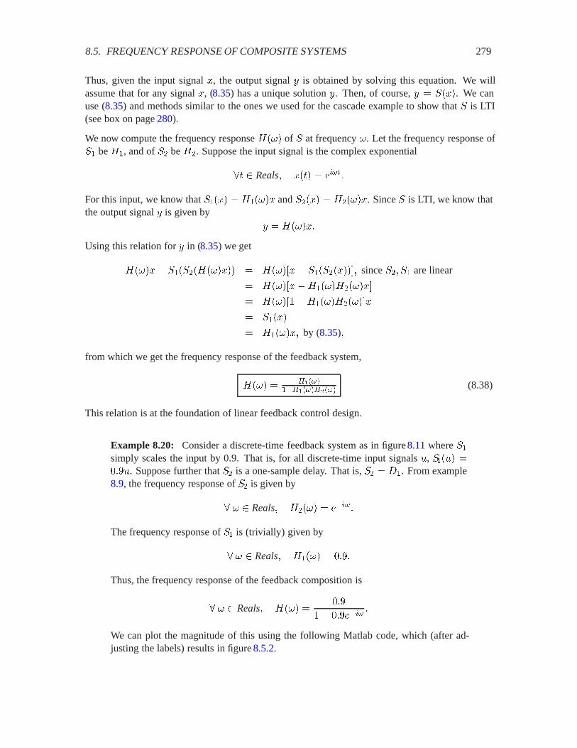
8.5. FREQUENCY RESPONSE OF COMPOSITE SYSTEMS 279
Thus, given the input signal �, the output signal � is obtained by solving this equation. We willassume that for any signal �, (8.35) has a unique solution �. Then, of course, � � .���. We canuse (8.35) and methods similar to the ones we used for the cascade example to show that . is LTI(see box on page 280).
We now compute the frequency response ;��� of . at frequency �. Let the frequency response of.� be ;�, and of .� be ;�. Suppose the input signal is the complex exponential
� Reals� ��� � �����
For this input, we know that .���� � ;����� and .���� � ;�����. Since . is LTI, we know thatthe output signal � is given by
� � ;�����
Using this relation for � in (8.35) we get
;����� .��.��;������ � ;������ .��.������� since .�� .� are linear
� ;������;����;������
� ;���� �;����;������
� .����
� ;������ by (8.35)�
from which we get the frequency response of the feedback system,
;��� � &� ����&� ��&� ��
(8.38)
This relation is at the foundation of linear feedback control design.
Example 8.20: Consider a discrete-time feedback system as in figure 8.11 where .�simply scales the input by 0.9. That is, for all discrete-time input signals 0, .��0� ���0. Suppose further that .� is a one-sample delay. That is, .� � ��. From example8.9, the frequency response of .� is given by
� � Reals� ;���� � �����
The frequency response of .� is (trivially) given by
� � Reals� ;���� � ���
Thus, the frequency response of the feedback composition is
� � Reals� ;��� ���
� �������
We can plot the magnitude of this using the following Matlab code, which (after ad-justing the labels) results in figure 8.5.2.

280 CHAPTER 8. FREQUENCY RESPONSE
Probing further: Feedback systems are LTI
To show that . in figure 8.11 is time-invariant we must show that for any � Reals,
.��( ���� � �( �.���� � �( ���� (8.36)
that is, we must show that �( ��� is the output of . when the input is �( ���. Nowthe left-hand side of (8.35) with � replaced by �( ��� is
�( ���� .��.���( ����� � �( �����( �.��.������
since .� and .� are time-invariant
� �( �� � .��.������� since �( is linear�
� �( �.������ by (8.35)
� .���( ����� since .� is time-invariant
so that �( ��� is indeed the solution of (8.35) when the input is �( ���. This proves(8.36).
Linearity is shown in a similar manner. Let � be any complex number. To showthat �� is the output when the input is ��, we evaluate the left-hand side of (8.35)at ��,
�� � .��.������ � �� � �.��.������ since .� and .� are linear
� ��� � .��.������
� �.����� by (8.35)
� .������ since .� is linear
which shows that .���� � �.���.
Now suppose / is another input and � � .�/� is the corresponding output, i.e.
� � .��.����� � .��/�� (8.37)
We evaluate the left-hand side of (8.35) at � � �,
�� � ��� .��.��� � ��� � �� � .��.������ � �� � .��.������
since .� and .� are linear
� .���� � .��/�� by (8.35) and (8.37)
� .����/�� since .� is linear
and so .��� /� � � � � � .��� � .���.

8.5. FREQUENCY RESPONSE OF COMPOSITE SYSTEMS 281
0 0.5 1 1.5 2 2.5 3 3.50
1
2
3
4
5
6
7
8
9
frequency (radians/sample)
ampl
itude
res
pons
e
Figure 8.12: The magnitude response of the feedback composition of ex-ample 8.20.
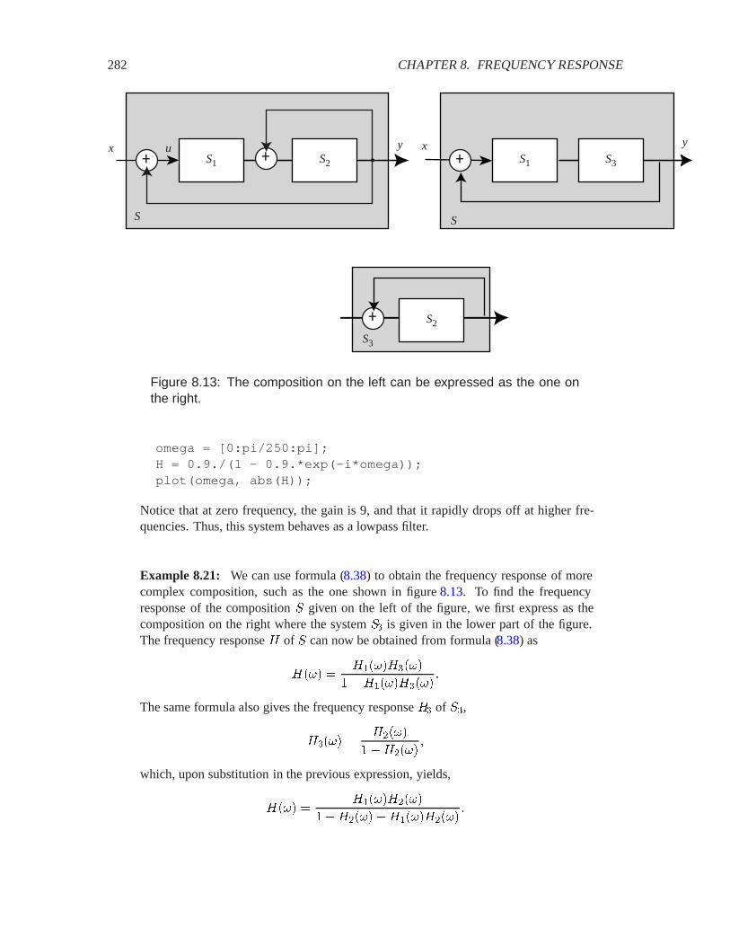
282 CHAPTER 8. FREQUENCY RESPONSE
S1 S2
S
x y
+u + S1 S3
x y
+
S
S2+S3
Figure 8.13: The composition on the left can be expressed as the one onthe right.
omega = [0:pi/250:pi];H = 0.9./(1 - 0.9.*exp(-i*omega));plot(omega, abs(H));
Notice that at zero frequency, the gain is 9, and that it rapidly drops off at higher fre-quencies. Thus, this system behaves as a lowpass filter.
Example 8.21: We can use formula (8.38) to obtain the frequency response of morecomplex composition, such as the one shown in figure 8.13. To find the frequencyresponse of the composition . given on the left of the figure, we first express as thecomposition on the right where the system .� is given in the lower part of the figure.The frequency response ; of . can now be obtained from formula (8.38) as
;��� �;����;����
�;����;�����
The same formula also gives the frequency response ;� of .�,
;���� �;����
�;�����
which, upon substitution in the previous expression, yields,
;��� �;����;����
�;�����;����;�����

8.6. SUMMARY 283
8.6 Summary
Linear time-invariant systems have a particularly nice property: if the input is a sinusoid, then theoutput is a sinusoid of the same frequency. Moreover, if the input is a sum of two sinusoids, thenthe output will be a sum of two sinusoids with the same frequencies as the input sinusoids. Eachsinusoid is scaled and shifted in phase by the system. The scaling and phase shift, as a function offrequency, is called the frequency response of the system.
It turns out that mathematically, this phenomenon is easiest to analyze using complex exponentialsinstead of real-valued sinusoids. The reason for this is that the phase shift and scaling togetheramount to simple multiplication of the complex exponential by a complex constant. If an inputis represented as a sum of complex exponentials (a form of the Fourier series), then the output issimply the same Fourier series with each term of the series scaled by a complex constant. Thesescaling constants, viewed as a function of frequency, are the frequency response of the system.
Composing LTI system becomes particularly easy. The frequency response of the cascade of twoLTI systems is simply the product of the frequency responses of the individual systems. This simplefact can be used to quickly ascertain the frequency response of complicated compositions.
Exercises
Each problem is annotated with the letter E, T, C which stands for exercise, requires some thought,requires some conceptualization. Problems labeled E are usually mechanical, those labeled T re-quire a plan of attack, those labeled C usually have more than one defensible answer.
1. E Find � Complexso that
� ���,�� ����� �������� � ������ �����
where �� is the complex conjugate of �.
2. E Plot the function ��Reals� Realsgiven by
� � Reals� ���� � Im�� �����)���You are free to choose a reasonable interval for your plot, but be sure it includes � � .
3. E This exercise explores the fact that a delay in a sinewave causes a phase shift. That is, forany real numbers � and �, there is a phase shift < Realssuch that for all Reals,
������� ��� � ������ <��
Give < in terms of �� �. What are the units of �� �� <? Hint: The argument to the sin functionhas units of radians.
4. E Let � � Reals� Reals. Show that � is periodic with period ( if and only if �#��� � �.Now show that if . is a time-invariant system and � is a periodic signal, then .��� is alsoperiodic with period (.
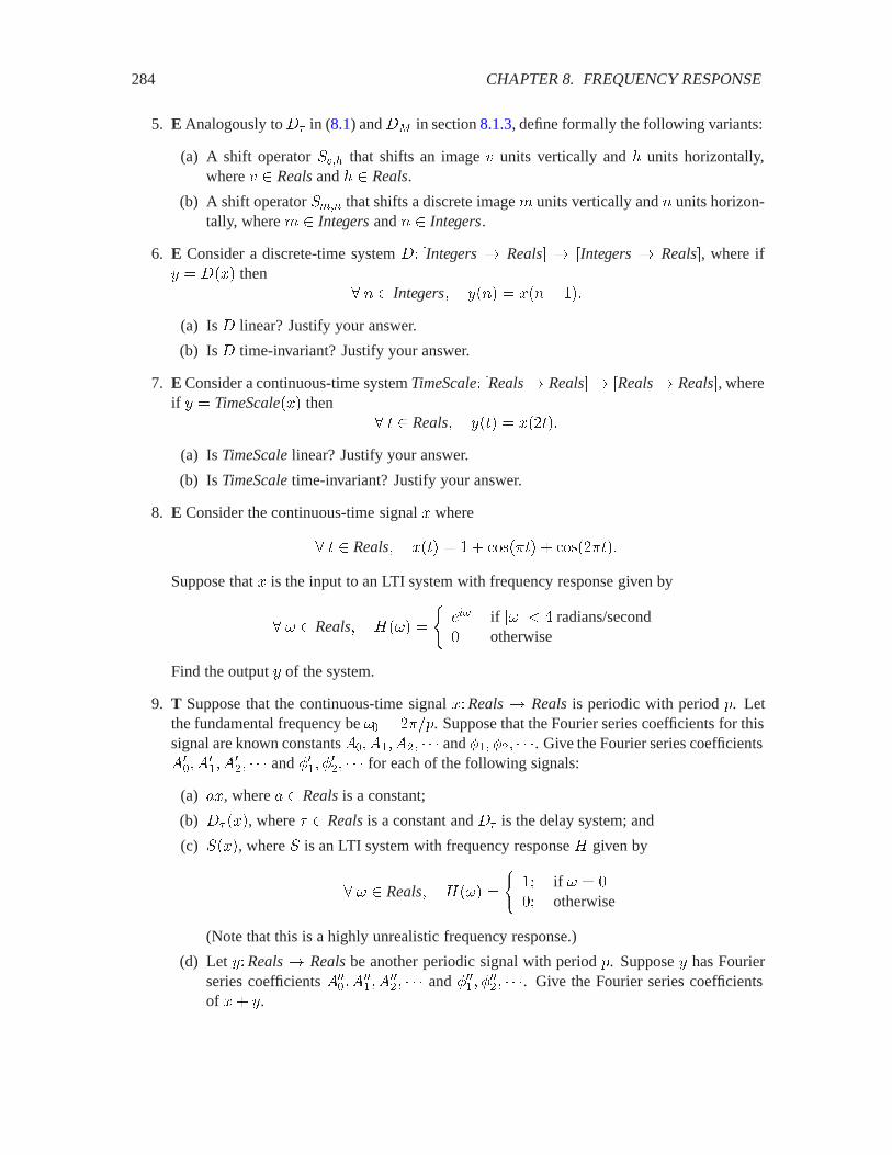
284 CHAPTER 8. FREQUENCY RESPONSE
5. E Analogously to �( in (8.1) and �� in section 8.1.3, define formally the following variants:
(a) A shift operator .,�- that shifts an image " units vertically and � units horizontally,where " Realsand � Reals.
(b) A shift operator .��� that shifts a discrete image ' units vertically and � units horizon-tally, where ' Integersand � Integers.
6. E Consider a discrete-time system �� �Integers� Reals� � �Integers� Reals�, where if� � ���� then
� � Integers� ���� � ���� ��
(a) Is � linear? Justify your answer.
(b) Is � time-invariant? Justify your answer.
7. E Consider a continuous-time system TimeScale� �Reals� Reals�� �Reals� Reals�, whereif � � TimeScale��� then
� Reals� ��� � �����
(a) Is TimeScalelinear? Justify your answer.
(b) Is TimeScaletime-invariant? Justify your answer.
8. E Consider the continuous-time signal � where
� Reals� ��� � � ������ � ��������
Suppose that � is the input to an LTI system with frequency response given by
� � Reals� ;��� �
���� if ��� ) � radians/second otherwise
Find the output � of the system.
9. T Suppose that the continuous-time signal ��Reals� Realsis periodic with period (. Letthe fundamental frequency be �� � ���(. Suppose that the Fourier series coefficients for thissignal are known constants ��� ��� ��� and <�� <�� . Give the Fourier series coefficients���� �
��� �
��� and <��� <
��� for each of the following signals:
(a) ��, where � Realsis a constant;
(b) �( ���, where � Realsis a constant and �( is the delay system; and
(c) .���, where . is an LTI system with frequency response ; given by
� � Reals� ;��� �
�% if � � % otherwise
(Note that this is a highly unrealistic frequency response.)
(d) Let ��Reals� Realsbe another periodic signal with period (. Suppose � has Fourierseries coefficients ���
�� ���� � �
��� � and <��� � <
��� � . Give the Fourier series coefficients
of �� �.
8.6. SUMMARY 285
10. E Consider discrete-time systems with input �� Integers� Realsand output �� Integers�Reals. Each of the following defines such a system. For each, indicate whether it is linear(L), time-invariant (TI), both (LTI), or neither (N).
(a) � � Integers� ���� � ���� � ������ �
(b) � � Integers� ���� � ������������
(c) � � Integers� ���� � ��������������
(d) � � Integers� ���� � ��������������� � ���� ��
(e) � � Integers� ���� � ���� � ��������
(f) � � Integers� ���� � ���� � ������ ���
11. E Suppose that the frequency response of a discrete-time LTI system . is given by
;��� � ��������
where � has units of radians/sample. Suppose the input is the discrete-time signal � given by� � Integers� ���� � . Give a simpleexpression for � � .���.
12. T Find the smallest positive integer � such that
�����
����)�� � �
Hint: Note that the term being summed is a periodic function of 6. What is its period? Whatis the sum of a complex exponential over one period?
13. T Consider a continuous-time periodic signal � with fundamental frequency �� � ra-dian/second. Suppose that the Fourier series coefficients (see (7.4)) are
�� �
� 6 � � � 4� � otherwise
and for all 6 Naturals�, <� � .
(a) Find the Fourier series coefficients �� for all 6 Integers(see (8.29)).
(b) Consider a continuous-time LTI system Filter � �Reals� Reals� � �Reals� Reals�,with frequency response
;��� � ����������
Find � � Filter���. I.e., give a simple expression for ��� that is valid for all Reals.
(c) For � calculated in (b), find the fundamental frequency in radians per second. I.e., findthe largest ��� 2 such that
� Reals� ��� � ��� �������
286 CHAPTER 8. FREQUENCY RESPONSE
14. T Consider a continuous-time LTI system .. Suppose that when the input � is given by
� ���,�� ��� �
�� if � ) � otherwise
then the output � � .��� is given by
� ���,�� ��� �
�� if � ) �� otherwise
Give an expression and a sketch for the output of the same system if the input is
(a)
� ���,�� ���� �
����
� if � ) �� if � ) �� otherwise
(b)
� ���,�� ���� �
�� if � ) ��� otherwise
15. T Suppose that the frequency response ; of a discrete-time LTI system Filter is given by:
� � ���� ��� ;��� � ����
where � has units of radians/sample. Note that since a discrete-time frequency responseis periodic with period ��, this definition implicitly gives ;��� for all � Reals. Givesimple expressions for the output � when the input signal � � Integers� Realsis such that� � Integerseach of the following is true:
(a) ���� � ���������.
(b) ���� � �.
(c) ���� �
��� � even�� � odd
16. T Consider a continuous-time LTI system .. Suppose that when the input is given by
��� �
������� � )
otherwise
then the output � � .��� is given by
��� �
�������� � ) ������� �� � ) � otherwise
for all Reals.
8.6. SUMMARY 287
(a) Carefully sketch these two signals.
(b) Give an expression and a sketch for the output of the same system if the input is
��� �
�������� � ) � ������� �� � ) � otherwise
�
17. T Suppose you are given the building blocks shown below for building block diagrams:
HW Gg
These blocks are defined as follows:
� An LTI system ;. � �Reals� Reals� � �Reals� Reals� that has a rectangular fre-quency response given by
� � Reals� ;��� �
� �7 ) � ) 7 otherwise
where 7 is a parameter you can set.
� A gain block 9/� �Reals� Reals�� �Reals� Reals� where if � � ����, then
� Reals� ��� � ����
where � Realsis a parameter you can set.
� An adder, which can add two continuous-time signals. Specifically, Add� �Reals�Reals�� �Reals� Reals�� �Reals� Reals� such that if � � Add���� ��� then
� Reals� ��� � ���� � �����
Use these building blocks to construct a system with the frequency response shown below:
H(ω)
ω
1
2
1 2 0 −1−2
18. T Let 0 be a discrete-time signal given by
� � Integers� 0��� �
� � � otherwise

288 CHAPTER 8. FREQUENCY RESPONSE
This is the unit step signal, which we saw before in (2.15). Suppose that a discrete-timesystem ; that is known to be LTI is such that if the input is 0, the output is � � ;�0� givenby
� � Integers� ���� � �0����
This is called the step response of the system. Find a simple expression for the output / �;�(� when the input is ( given by
� � Integers� (��� �
�� � � ) � otherwise
Sketch /.
19. T Suppose you are given the Fourier series coefficients ���������� ��� for a periodicsignal ��Reals� Realswith period (. Find the fundamental frequency and the Fourier seriescoefficients of the following signals in terms of those of �.
(a) � such that � Reals� ��� � ����, for some positive real number �.
(b) / such that � Reals� /�� � ��������, where �� � ���(.
(c) � such that � Reals� ��� � ��� �������, where �� � ���(.
20. Analogously to the box on page 274, show that the formula (8.33) for the discrete Fourierseries coefficients is valid.
21. C Consider a system Squarer� �Reals� Reals�� �Reals� Reals�, where if � � Squarer���then
� Reals� ��� � �������
(a) Show that this system is memoryless.
(b) Show that this system is not linear.
(c) Show that this system is time invariant.
(d) Suppose that the input � is given by
� Reals� ��� � !4�����
for some fixed �. Show that the output � contains a component at frequency ��.

Chapter 9
Filtering
Linear time invariant systems have the property that if the input is described as a sum of sinusoids,then the output is a sum of sinusoids of the same frequency. Each sinusoidal component will typ-ically be scaled differently, and each will be subjected to a phase change, but the output will notcontain any sinusoidal components that are not also present in the input. For this reason, an LTIsystem is often called a filter. It can filter out frequency components of the input, and also enhanceother components, but it cannot introduce components that are not already present in the input. Itmerely changes the relative amplitudes and phases of the frequency components that are present inthe inputs.
LTI systems arise in two circumstances in an engineering context. First, they may be used as a modelof a physical system. Many physical systems are accurately modeled as LTI systems. Second, theymay present an ideal for an engineered system. For example, they may specify the behavior that anelectronic system is expected to exhibit.
Consider for example an audio system. The human ear hears frequencies in the range of about 30 to20,000 Hz, so a specification for a high fidelity audio system typically requires that the frequencyresponse be constant (in magnitude) over this range. The human ear is relatively insensitive tophase, so the same specification may say nothing about the phase response (the argument, or angleof the frequency response). An audio system is free to filter out frequencies outside this range.
Consider an acoustic environment, a physical context such as a lecture hall where sounds are heard.The hall itself alters the sound. The sound heard by your ear is not identical to the sound cre-ated by the lecturer. The room introduces echoes, caused by reflections of the sound by the walls.These echoes tend to occur more for the lower frequency components in the sound than the higherfrequency components because the walls and objects in the room tend to absorb higher frequencysounds better. Thus, the lower frequency sounds bounce around in the room, reinforcing each other,while the higher frequency sounds, which are more quickly absorbed, become relatively less pro-nounced. In an extreme circumstance, in a room where the walls are lined with shag carpeting, forexample, the higher frequency sounds are absorbed so effectively that the sound gets muffled by theroom.
The room can be modeled by an LTI system where the frequency response ;��� is smaller in
289
290 CHAPTER 9. FILTERING
magnitude for large � than for small �. This is a simple form of distortion introduced by a channel(the room), which in this case carries a sound from its transmitter (the lecturer) to its receiver (thelistener). This form of distortion is called linear distortion, a shorthand for linear, time-invariantdistortion (the time invariance is left implicit).
A public address system in a lecture hall may compensate for the acoustics of the room by boostingthe high frequency content in the sound. Such a compensator is called an equalizer because itcorrects for distortion in the channel so that all frequencies are received equally well by the receiver.
In a communications system, a channel may be a physical medium, such as a pair of wires, thatcarries an electrical signal. That physical medium distorts the signal, and this distortion is often rea-sonably well approximated as linear and time invariant. An equalizer in the receiver compensatesfor this distortion. Unlike the audio example, however, such an equalizer often needs to compen-sate for the phase response, not just the magnitude response. Because the human ear is relativelyinsensitive to phase distortion, a public address system equalizer need not compensate for phasedistortion. But the wire pair may be carrying a signal that is not an audio signal. It may be, forexample, a modem signal.
Images may also be processed by LTI systems. Consider the three images shown in figure9.1. Thetop image is the original, undistorted image. The lower left image is blurred, as might result forexample from unfocused optics. The lower right image is, in a sense, the opposite of the blurredimage. Whereas the blurred image deemphasizes the patterns in the outfit, for example, the rightimage deemphasizes the regions of constant value, changing them all to a neutral gray.
For images, time is not the critical variable. Its role is replaced by two spatial variables, one in thehorizontal direction and one in the vertical direction. Thus, instead of LTI, we might talk aboutan image processing system being a linear, space-invariant (LSI) system. The blurred image isconstructed from the original by an LSI system that eliminates high (spatial) frequencies, passingunaltered the low frequencies. Such a system is called a lowpass filter. The lower right image isconstructed from the original by an LSI system that eliminates low frequencies, passing unalteredthe high frequencies. Such a system is called a highpass system. Both images were created usingAdobe Photoshop, although the blurred image could have been just as easily created by a defocusedlens.
9.1 Convolution
The frequency response of a system is a declarative description of the system. It tells us what it is,not how it works. It tells us, for example, that it is a lowpass filter, but it does not tell us whether it isa defocused lens or a computer program, much less telling us how the computer program works. Inthis chapter, we explore imperative descriptions of systems, and build up to detailed descriptions ofsoftware that can implement certain kinds of LTI (or LSI) systems. These imperative descriptionsare based on convolution.
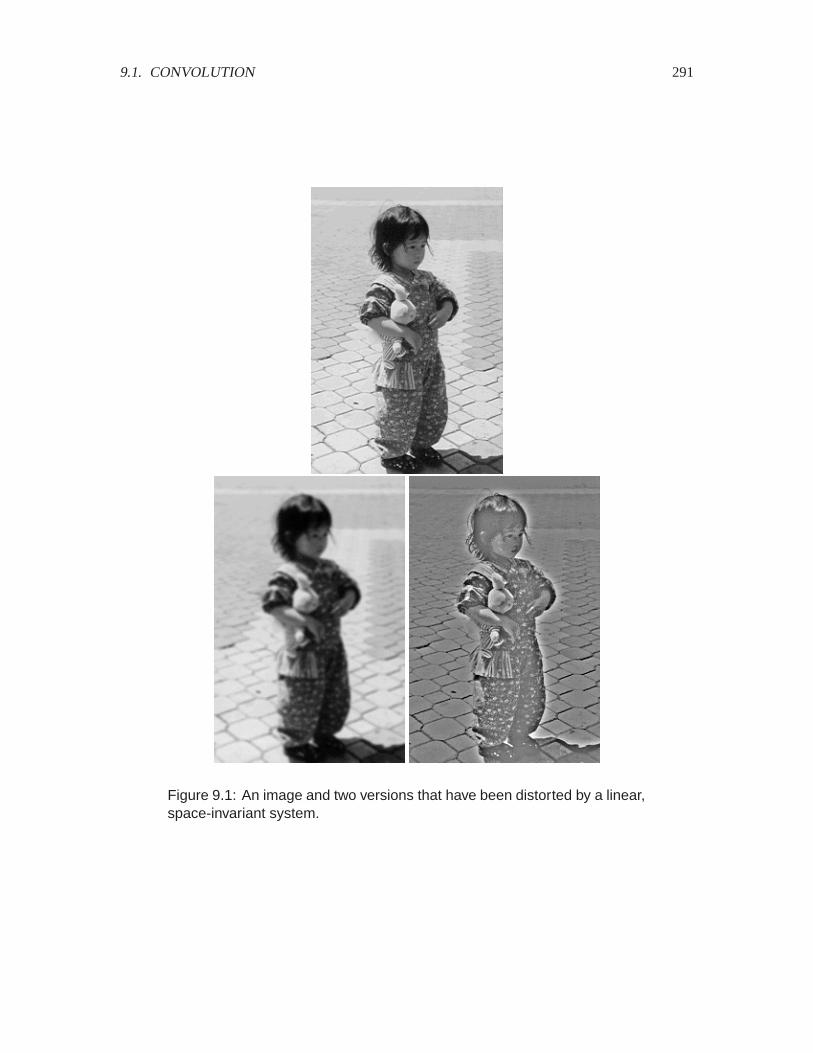
9.1. CONVOLUTION 291
Figure 9.1: An image and two versions that have been distorted by a linear,space-invariant system.
292 CHAPTER 9. FILTERING
9.1.1 Convolution sum and integral
For discrete-time signals the convolution operator is called the convolution sum, and for continuous-time signals it is called the convolution integral. We define these two operators now and note someimportant properties.
Let �� � �Integers� Reals� be two discrete-time signals. The convolution of � and � is thediscrete-time signal, denoted � � �, given by the convolution sum,
�� Integers� �� � ����� ���
������6����� 6�� (9.1)
We note two properties. First, the order in the convolution does not matter, � � � � � � �. Indeed,if in (9.1) we change the variables in the summation, letting ' � �� 6, we get
�� Integers� �� � ����� ���
����
��6����� 6�
���
����
����'���'��
Thus,
�� � ����� � �� � ������ (9.2)
This property is called commutativity of the convolution operator.1
Another property of convolution is linearity. That is, if �� ��� �� are three signals and �� and �� arereal numbers, then
� � ����� � ����� � ���� � ��� � ���� � ���� (9.3)
which may be checked directly by applying definition (9.1) to both sides.
We now use the convolution sum to define some LTI systems. Fix a discrete-time signal �, anddefine the system
.� �Integers� Reals�� �Integers� Reals�
by
� � �Integers� Reals�� .��� � � � ��Thus the output signal � � .��� corresponding to the input signal � is given by
� � Integers� ���� ���
����
��6����� 6��
1Matrix multiplication is an example of an operator that is not commutative, while matrix addition is. Since the sumof two matrices � and � (of the same size) does not depend on the order, i.e., � � � � � � � , the matrix sumis a commutative operator. However, the product of two matrices depends on the order, i.e., it is not always true that� �� � � �� , so the matrix product is not commutative.
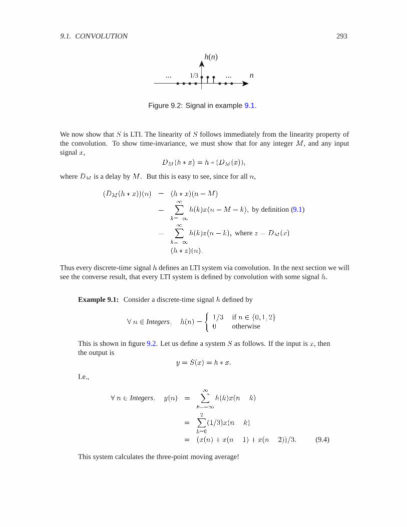
9.1. CONVOLUTION 293
h(n)
n...... 1/3
Figure 9.2: Signal in example 9.1.
We now show that . is LTI. The linearity of . follows immediately from the linearity property ofthe convolution. To show time-invariance, we must show that for any integer 3 , and any inputsignal �,
�� �� � �� � � � ��� �����
where �� is a delay by 3 . But this is easy to see, since for all �,
��� �� � ������ � �� � �����3�
���
����
��6���� �3 � 6�� by definition (9.1)
���
����
��6���� � 6�� where � � �� ���
� �� � ������
Thus every discrete-time signal � defines an LTI system via convolution. In the next section we willsee the converse result, that every LTI system is defined by convolution with some signal �.
Example 9.1: Consider a discrete-time signal � defined by
� � Integers� ���� �
��� if � �� � � otherwise
This is shown in figure 9.2. Let us define a system . as follows. If the input is �, thenthe output is
� � .��� � � � ��I.e.,
� � Integers� ���� ���
����
��6���� � 6�
���
���
������� � 6�
� ����� � ���� � � ���� ������ (9.4)
This system calculates the three-point moving average!
294 CHAPTER 9. FILTERING
We now turn to the continuous time case. Let �� � �Reals� Reals� be two continuous-timesignals. The convolution of � and � is the continuous-time signal, denoted � � �, given by theconvolution integral
� Reals� �� � ���� ��"
��������� ����� (9.5)
By a change of variable in the integral we can check that convolution again is commutative, i.e.,
� Reals� �� � ���� � �� � ����� (9.6)
and it is linear; i.e. if �� ��� �� are three continuous-time signals and ��� �� are real numbers, then
� � ����� � ����� � ���� � ��� � ���� � ���� (9.7)
Again fix � �Reals� Reals�, and define the system
.� �Reals� Reals�� �Reals� Reals�
by� � �Reals� Reals�� .��� � � � ��
Then in exactly the same way as for the discrete-time case, we can show that . is LTI.
Example 9.2: Consider a continuous-time signal � defined by
� Reals� ��� �
��� if �� �� otherwise
This is shown in figure 9.3. Let us define a system . as follows. If the input is �, thenthe output is
� � .��� � � � ��I.e,
� Reals� ��� �
����
������ � ����
�
�
���
��� ����� (9.8)
This system is the length-three continuous-time moving average!
Note that we are using the same symbol ‘*’ for the convolution sum and the convolution integral.The context will determine which operator is intended.
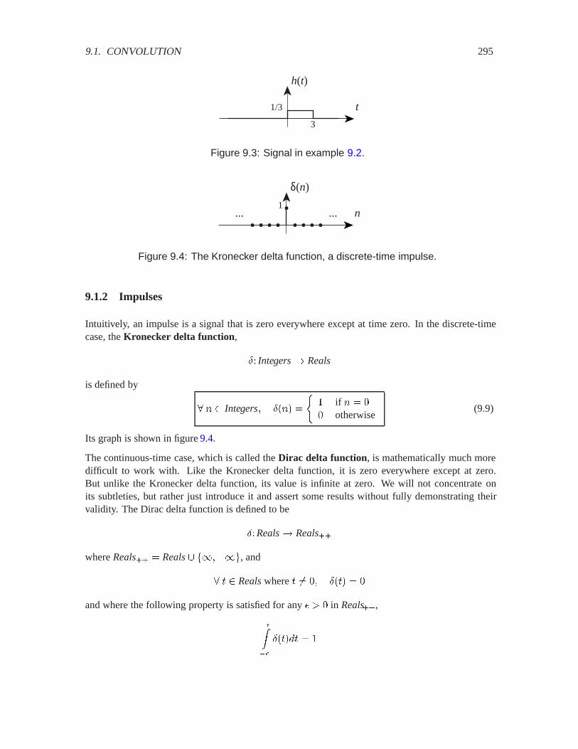
9.1. CONVOLUTION 295
h(t)
t1/3
3
Figure 9.3: Signal in example 9.2.
δ(n)
n......1
Figure 9.4: The Kronecker delta function, a discrete-time impulse.
9.1.2 Impulses
Intuitively, an impulse is a signal that is zero everywhere except at time zero. In the discrete-timecase, the Kronecker delta function,
� Integers� Reals
is defined by
� � Integers� ��� �
� if � � otherwise
(9.9)
Its graph is shown in figure 9.4.
The continuous-time case, which is called the Dirac delta function, is mathematically much moredifficult to work with. Like the Kronecker delta function, it is zero everywhere except at zero.But unlike the Kronecker delta function, its value is infinite at zero. We will not concentrate onits subtleties, but rather just introduce it and assert some results without fully demonstrating theirvalidity. The Dirac delta function is defined to be
�Reals� Reals��
where Reals�� � Reals� �����, and
� Realswhere �� � �� �
and where the following property is satisfied for any A 2 in Reals��,
0��0
��� �

296 CHAPTER 9. FILTERING
δ(t)
t1
Figure 9.5: The Dirac delta function, a continuous-time impulse.
For the latter property to be satisfied, clearly no finite value at � would suffice. This is why thevalue must be infinite at � . Notice that the Kronecker delta function has a similar property,
������
��� �
for any integer � 2 , but that in this case, the property is trivial. There is no mathematical subtlety.
The Dirac delta function is usually depicted as in figure 9.5. In any figure, of course, the infinitevalue at � cannot be shown directly. The figure suggests that infinite value with a vertical arrow.Next to the arrow is the weight of the delta function, ‘1’ in this case. In general, a Dirac deltafunction can be multiplied by any real constant �. Of course, this does not change its value at � ,which is infinite, nor does it change its value at �� , which is zero. What it does change is itsintegral,
0��0
���� � ��
Thus, although the impulse is still infinitely narrow and infinitely high, the area under the impulsehas been scaled by �.
9.1.3 Signals as sums of weighted delta functions
Any discrete-time signal �� Integers� Realscan be expressed as a sum of weighted Kroneckerdelta functions,
� � Integers� ���� ���
������6���� 6�. (9.10)
The 6th term in the sum is ��6����6�. This term, by itself, defines a signal that is zero everywhereexcept at � � 6, where it has value ��6�. This signal is called a weighted delta function becauseit is a (time shifted) delta function with a specified weight. Thus, any discrete-time signal is a sumof weighted delta functions, much the way that the Fourier series describes a signal as a sum ofweighted complex exponential functions.
Example 9.3: The signal � in example 9.1 can be written in terms of Kronecker deltafunctions,
� � Integers� ���� � ���� � ��� � � ��� ������
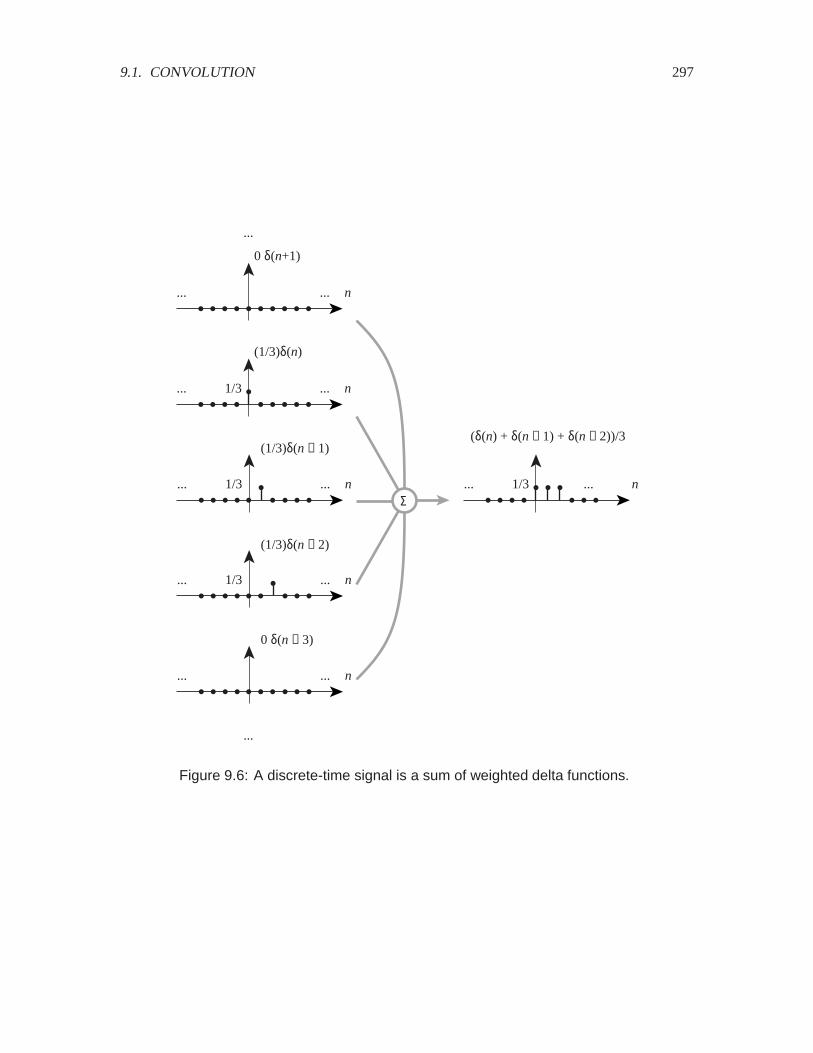
9.1. CONVOLUTION 297
n...... 1/3
(1/3)δ(n)
n...... 1/3
n...... 1/3
n...... 1/3
n......
0 δ(n+1)
n......
Σ
(1/3)δ(n − 1)
(1/3)δ(n − 2)
0 δ(n − 3)
...
...
(δ(n) + δ(n − 1) + δ(n − 2))/3
Figure 9.6: A discrete-time signal is a sum of weighted delta functions.

298 CHAPTER 9. FILTERING
This has the form of (9.10), and is illustrated in figure 9.6. It is described as a sum ofsignals where each signal contains only a single weighted impulse.
Equation (9.10) is sometimes called the sifting property of the Kronecker delta function because it“sifts out” the value of a function � at some integer �. That is, the infinite sum reduces to a singlenumber. This property can often be used to eliminate infinite summations in more complicatedexpressions.
The continuous-time version of this is similar, except that the sum becomes an integral (integration,after all, is just sum over a continuum). Given any signal ��Reals� Reals,
� Reals� ��� �
����
����� � ���� . (9.11)
Although this is mathematically much more subtle than the discrete-time case, it is very similar instructure. It describes a signal � as a sum (or more precisely, an integral) of weighted Dirac deltafunctions.
Example 9.4: The signal � in figure 9.3 and example 9.2 can be written as a sum (anintegral, actually) of weighted Dirac delta functions,
� Reals� ��� �
� �
������� � ����
�
� �
������ � �����
This has the form of (9.11).
Equation (9.11) is sometimes called the sifting property of the Dirac delta function, because itsifts out from the function � the value at a given time . The sifting property can often be used toeliminate integrals, since it replaces an integral with a single value.
9.1.4 Impulse response and convolution
Consider a discrete-time LTI system .� �Integers� Reals� � �Integers� Reals�. Define itsimpulse response � to be the output signal when the input signal is the Kronecker delta function(an impulse), � � .��, that is,
� � Integers� ���� � �.�������
Now let � be any input signal, and let � � .��� be the corresponding output signal. In (9.10), � isgiven as sum of components, where each component is a weighted delta function. Since . is LTI,the output can be given as a sum of the responses to these components. Each component is a signal

9.1. CONVOLUTION 299
��6��� � 6� for fixed k, and the response to this signal is ��6���� � 6�. The response to a scaledand delayed impulse will be a scaled and delayed impulse response. Thus, the overall output is
� � Integers� ���� ���
������6����� 6� � �� � ����� � �� � �����.
Thus, the output of any discrete-time LTI system is given by the convolution of the input signal andthe impulse response.
Example 9.5: The three-point moving average system . of example 9.1 has impulseresponse
� � Integers� ���� � ���� � ��� � � ��� ������
This can be determined from (9.4) by just letting the input be � � Æ. The impulseresponse, after all, is defined to be the output when the input is an impulse. The impulseresponse is shown in figure 9.2.
Consider now a continuous-time LTI system .� �Reals� Reals� � �Reals� Reals�. Defineits impulse response to be the output signal � when the input signal is the Dirac delta function,� � .��, i.e.,
� Reals� ��� � .�����
Now let � be any input signal and let � � .���, be the corresponding output signal. By the siftingproperty we can express � as the sum (integral) of weighted delta functions,
��� �
� �
������� � �����
Since . is LTI, the output is a sum (integral) of the responses to each of the components (theintegrand for fixed � ), or
� Reals� ��� ��"
�������� � ���� � �� � ���� � �� � ����. (9.12)
Thus,
The output of any continuous-time LTI system is given by the convolution of theinput signal and the impulse response.
Example 9.6: The length-three continuous-time moving average system . of example9.2 has impulse response
� Reals� ��� �
��� if �� �� otherwise
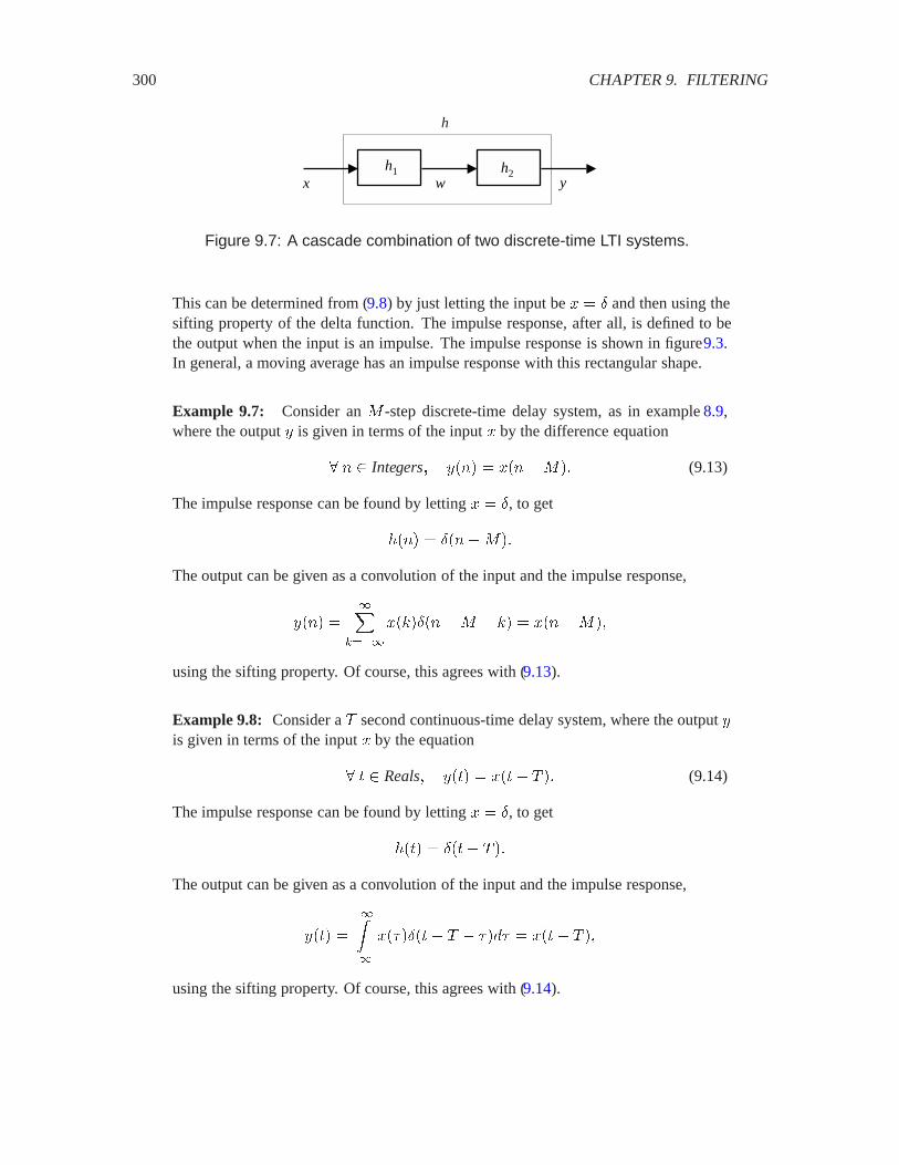
300 CHAPTER 9. FILTERING
x
h
wh1 h2
y
Figure 9.7: A cascade combination of two discrete-time LTI systems.
This can be determined from (9.8) by just letting the input be � � Æ and then using thesifting property of the delta function. The impulse response, after all, is defined to bethe output when the input is an impulse. The impulse response is shown in figure9.3.In general, a moving average has an impulse response with this rectangular shape.
Example 9.7: Consider an 3 -step discrete-time delay system, as in example 8.9,where the output � is given in terms of the input � by the difference equation
� � Integers� ���� � ����3�� (9.13)
The impulse response can be found by letting � � Æ, to get
���� � ���3��
The output can be given as a convolution of the input and the impulse response,
���� ���
����
��6��� �3 � 6� � ����3��
using the sifting property. Of course, this agrees with (9.13).
Example 9.8: Consider a second continuous-time delay system, where the output �is given in terms of the input � by the equation
� Reals� ��� � ��� �� (9.14)
The impulse response can be found by letting � � Æ, to get
��� � �� ��
The output can be given as a convolution of the input and the impulse response,
��� �
����
����� � � ���� � ��� ��
using the sifting property. Of course, this agrees with (9.14).
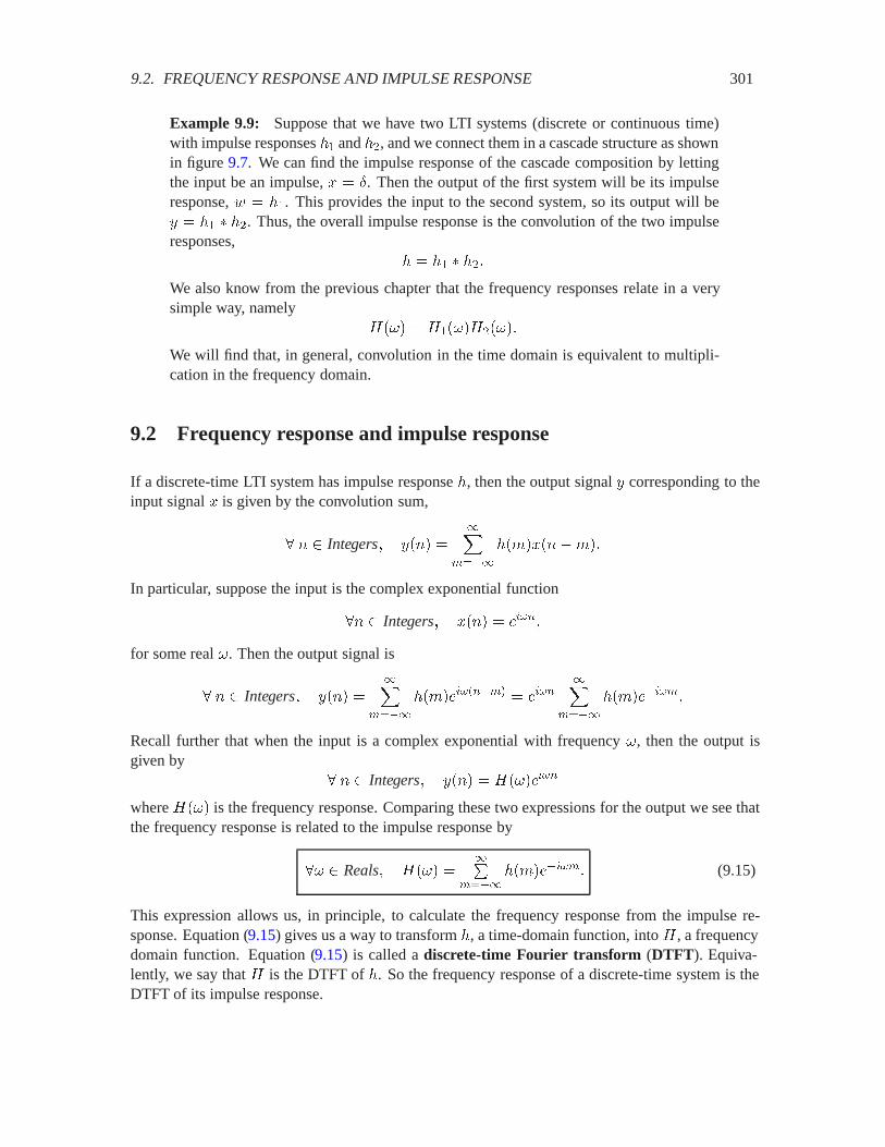
9.2. FREQUENCY RESPONSE AND IMPULSE RESPONSE 301
Example 9.9: Suppose that we have two LTI systems (discrete or continuous time)with impulse responses �� and ��, and we connect them in a cascade structure as shownin figure 9.7. We can find the impulse response of the cascade composition by lettingthe input be an impulse, � � Æ. Then the output of the first system will be its impulseresponse, / � ��. This provides the input to the second system, so its output will be� � �� � ��. Thus, the overall impulse response is the convolution of the two impulseresponses,
� � �� � ���We also know from the previous chapter that the frequency responses relate in a verysimple way, namely
;��� � ;����;�����
We will find that, in general, convolution in the time domain is equivalent to multipli-cation in the frequency domain.
9.2 Frequency response and impulse response
If a discrete-time LTI system has impulse response �, then the output signal � corresponding to theinput signal � is given by the convolution sum,
� � Integers� ���� ���
����
��'�����'��
In particular, suppose the input is the complex exponential function
�� Integers� ���� � �����
for some real �. Then the output signal is
� � Integers� ���� ���
����
��'���� ���� � ������
����
��'�������
Recall further that when the input is a complex exponential with frequency �, then the output isgiven by
� � Integers� ���� � ;�������
where ;��� is the frequency response. Comparing these two expressions for the output we see thatthe frequency response is related to the impulse response by
�� Reals� ;��� ���
������'������� (9.15)
This expression allows us, in principle, to calculate the frequency response from the impulse re-sponse. Equation (9.15) gives us a way to transform �, a time-domain function, into ; , a frequencydomain function. Equation (9.15) is called a discrete-time Fourier transform (DTFT). Equiva-lently, we say that ; is the DTFT of �. So the frequency response of a discrete-time system is theDTFT of its impulse response.
302 CHAPTER 9. FILTERING
Example 9.10: Consider the 3 -step delay from example 9.7. Its impulse response is
� � Integers� ���� � ���3��
We can find the frequency response by calculating the DTFT,
� � Reals� ;��� ���
����
��'������
���
����
�'�3������
� �����
where the last step follows from the sifting property. This same result was obtainedmore directly in example 8.9. Note that the magnitude response is particularly simple,
�;���� � �
This is intuitive. An 3 -step delay does not change the magnitude of any complexexponential input. It only shifts its phase.
Notice from (9.15) that
If � is real-valued then ;����� � ;��� (9.16)
(just conjugate both sides of (9.15) and evaluate at ��). This property is called conjugate symme-try. It implies
�;����� � �;����� (9.17)
This says that for any LTI system with a real-valued impulse response, a complex exponential withfrequency � experiences the same amplitude change as a complex exponential with frequency ��.
Notice further from (9.15) that
� � Reals� ;�� � ��� � ;���� (9.18)
I.e., the DTFT is periodic with period ��. This says that a complex exponential with frequency �experiences the same amplitude and phase change as a complex exponential with frequency ����.This should not be surprising since the two complex exponentials are in fact identical,
� � Integers� �� ���)�� � �������)� � �����
because ���)� � for any integer �.
The continuous-time version proceeds in the same way. Let . be a continuous-time system withimpulse response �. Then the output signal � corresponding to an input signal � is given by
� Reals� ��� �
� �
����� ���������
9.2. FREQUENCY RESPONSE AND IMPULSE RESPONSE 303
In particular, if the input signal is the complex exponential,
� Reals� ��� � �����
then the output signal is
��� �
� �
����� ��(������� � ����
� �
������(�������
The output is also given by ��� � ;������� where ;��� is the frequency response, and so wehave
;��� ��"
������������ (9.19)
So, given its impulse response, we can calculate the frequency response of a continuous-time LTIsystem by evaluating the integral (9.19). Like the DTFT, this integral transforms a time-domainsignal � into a frequency-domain signal ; . It is called the continuous-time Fourier transform(CTFT), or more commonly, simply the Fourier transform (FT). Thus the frequency response ;of a continuous-time LTI system is just the CTFT of its impulse response �.
Example 9.11: Consider the second delay from example 9.8. Its impulse responseis
��� � �� ��
We can find the frequency response by calculating the CTFT,
;��� �
����
���������
�
����
�� �������
� �����
where the last step follows from the sifting property. Note that the magnitude responseis particularly simple,
�;���� � �
This is intuitive. A second delay does not change the magnitude of any complexexponential input. It only shifts its phase.
Notice from (9.19) that the CTFT is also conjugate symmetric if � is real,
;����� � ;��� (9.20)
�;����� � �;����� (9.21)
304 CHAPTER 9. FILTERING
9.3 Causality
A system is causal if the output value at a particular time depends only on the input values at thattime or before. For LTI systems, if we examine the convolution sum,
���� ���
����
��'�����'��
for a causal system it must be true that ��'� � for all ' ) . Were this not true, there would benon-zero terms in the sum with ' ) , and those terms would involve a future sample of the input,����'�. Conversely, if ��'� � for all ' ) , then the system is causal since the sum for ����will involve only previous input values, ����� ���� �� ��� � ��� .Causality is an important practical property of a system that receives its data in real time (physicaltime). Such systems cannot possibly look ahead in time, at least not until someone invents a timemachine. However, there are many situations where causality is irrelevant. A system that processesstored data, such as digital audio of a compact disk or audio files in a computer, has no difficultylooking ahead in “time.”
9.4 Finite impulse response (FIR) filters
Consider an LTI system .� �Integers � Reals� � �Integers � Reals� with impulse response�� Integers� Realsthat has the properties
���� � if � ) � and ���� � if � � 1�
where 1 is some positive integer. Such a system is called a finite impulse response (FIR) systembecause the interesting part (the non-zero part) of the impulse response is finite in extent. Becauseof that property, the convolution sum becomes a finite sum,
���� ���
����
����'���'� �1������
����'���'�� (9.22)
1 is the length of the impulse response.
This sum, since it is finite, is convenient to work with. It can be used to define a procedure forcomputing the output of an FIR system given its input. This makes it easy to implement on a com-puter. We will see that it is also reasonably straightforward to implement certain infinite impulseresponse (IIR) filters on a computer.
A continuous-time finite impulse response could be defined, but in practice, continuous-time sys-tems rarely have finite impulse responses, so there is not as much motivation for doing so. More-over, even though the convolution integral acquires finite limits, this does not make it any morecomputable. Computing integrals on a computer is a difficult proposition whether the limits arefinite or not.

9.4. FINITE IMPULSE RESPONSE (FIR) FILTERS 305
Probing further: Causality
We can give a much more general and formal definition of causality that does notrequire a system to be LTI. Consider a system .� �� � �� � �� � �� thatoperates on signals of type �� � ��. Assume � is an ordered set and � is anyordinary set. An ordered set is one with relations “)” and “2” where for any twoelements � and �, one of the following assertions must be true:
� � �� � 2 �� or � ) ��
Examples of ordered sets are Integersand Reals.
An example of a set that is not an ordered set is Integers� Integerswhere we definethe ordering relation “)” so that ��� �� ) �!� �� if � ) ! and � ) !, and we similarlydefine “2”. Under these definitions, for the elements (1,2) and (2,1), none of theabove assertions is true, so the set is not ordered.
However, we could define the ordering relation “)” so that ��� �� ) �!� �� if one ofthe following is true:
� ) ! or
� � !� and � ) !�
The relation “2” could be similarly defined. Under these definitions, the set isordered.
Define a function Prefix�� ��� ��� ��� � �� that extracts a portion of a signalup to �. Formally, �� � � such that � �� if � � and � � . Then for all� ��� �� and for all ��, �Prefix������� � ���.
A system . is causal if for all � and for all �� � ��� ��
Prefix���� � Prefix����� Prefix��.���� � Prefix��.�����
The symbol “�” reads “implies.” In words, the system is causal if when two inputsignals have the same prefix up to time , it follows that the two correspondingoutput signals have the same prefix up to time .

306 CHAPTER 9. FILTERING
Example 9.12: We have seen in example 9.1 a 3-point moving average. An 1-pointmoving average system with input � has output � given by
���� �
1
1������
����'��
The output at index � is the average of the most recent 1 inputs. Such a filter is widelyused on Wall Street to try to detect trends in stock market prices. We can study itsproperties. First, it is easy to see that it is an LTI system. In fact, it is an FIR systemwith impulse response
���� �
��1 if � � ) 1 otherwise
To see this, just let � � Æ. The frequency response is the DTFT of this impulse re-sponse,
;��� ���
����
��'������
�
1
1������
������
With the help of the useful identity2
1������
�� �� �1
� �(9.23)
we can write the frequency response as
;��� �
1
�� ����1
� ����
�
where we have let � � ����. We can plot the magnitude of the frequency responseusing Matlab as follows (for 1 � �):3
L = 4;omega = [-pi:pi/250:pi];H = (1/L)*(1-exp(-i*omega*L))./(1-exp(-i*omega));plot(omega, abs(H));xlabel(’frequency in radians/sample’);
2You can verify the identity by multiplying both sides by �� �.3This issues a “divide by zero” warning, but yields a correct plot nonetheless. The magnitude of the frequency
response at � � � is 1, as you can verify using L’Hopital’s rule.
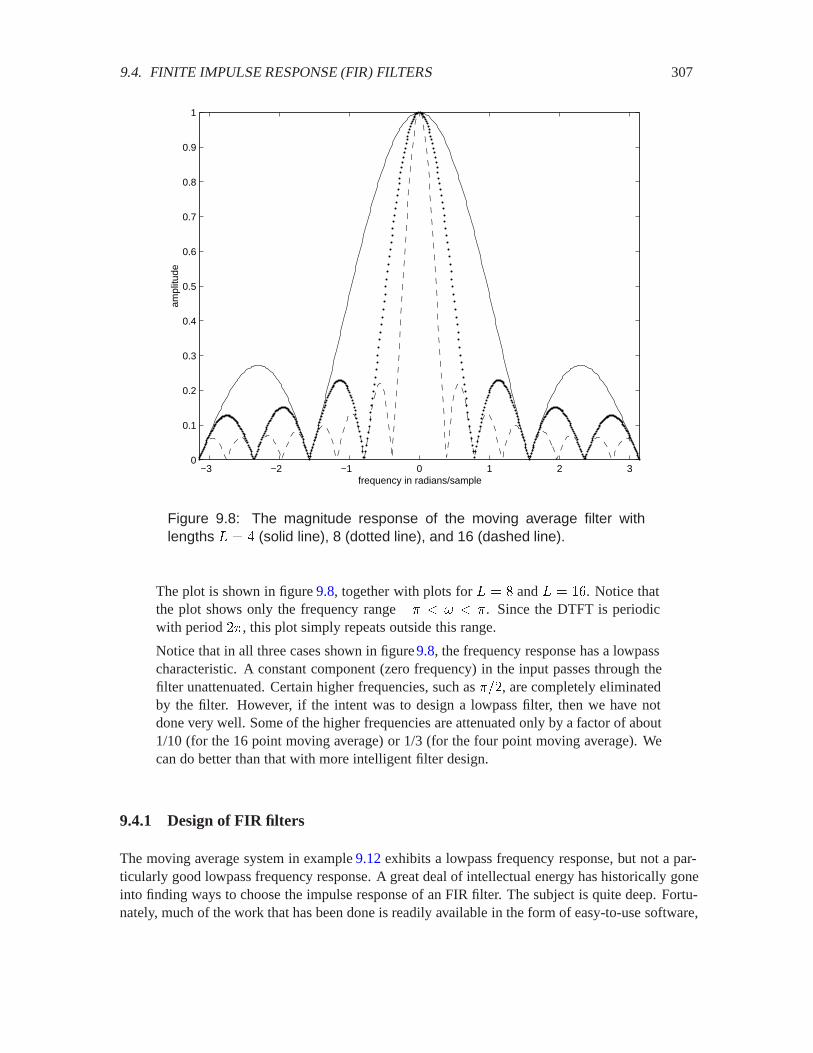
9.4. FINITE IMPULSE RESPONSE (FIR) FILTERS 307
−3 −2 −1 0 1 2 30
0.1
0.2
0.3
0.4
0.5
0.6
0.7
0.8
0.9
1
frequency in radians/sample
ampl
itude
Figure 9.8: The magnitude response of the moving average filter withlengths 1 � � (solid line), 8 (dotted line), and 16 (dashed line).
The plot is shown in figure 9.8, together with plots for 1 � � and 1 � . Notice thatthe plot shows only the frequency range �� ) � ) �. Since the DTFT is periodicwith period ��, this plot simply repeats outside this range.
Notice that in all three cases shown in figure 9.8, the frequency response has a lowpasscharacteristic. A constant component (zero frequency) in the input passes through thefilter unattenuated. Certain higher frequencies, such as ���, are completely eliminatedby the filter. However, if the intent was to design a lowpass filter, then we have notdone very well. Some of the higher frequencies are attenuated only by a factor of about1/10 (for the 16 point moving average) or 1/3 (for the four point moving average). Wecan do better than that with more intelligent filter design.
9.4.1 Design of FIR filters
The moving average system in example 9.12 exhibits a lowpass frequency response, but not a par-ticularly good lowpass frequency response. A great deal of intellectual energy has historically goneinto finding ways to choose the impulse response of an FIR filter. The subject is quite deep. Fortu-nately, much of the work that has been done is readily available in the form of easy-to-use software,
308 CHAPTER 9. FILTERING
so one does not need to be particularly knowledgeable about these techniques to be able to designgood FIR filters.
Example 9.13: Matlab’s filter design facilities in its DSP toolbox provide some well-studied algorithms for filter design. For example,
>> h = remez(7,[0,0.125,0.25,1],[1,1,0,0])
h =
Columns 1 through 6
0.0849 0.1712 0.1384 0.1912 0.1912 0.1384
Columns 7 through 8
0.1712 0.0849
This returns the impulse response of a length 8 FIR lowpass filter. The arguments tothe remez function specify the filter by outlining approximately the desired frequencyresponse. You can use Matlab’s on-line help to get the details, but in brief, the argu-ments above define a passband (a region of frequency where the gain is roughly 1) anda stopband (a region of frequency where the gain is roughly 0). The first argument, 7specifies that the length of the filter should be 8 (you will have to ask The MathWorkswhy this is off by one). The second argument, [0,0.125,0.25,1], specifies thatthe first frequency band begins at 0 and extends to ���� radians/sample, and thatthe second band begins at ���� and extends to � radians/sample. (The � factor is leftoff.) The unspecified band, from ���� to ����, is a “don’t care” region, a transitionband that allows for a gradual transition between the passband and the stopband.
The last argument, [1,1,0,0], specifies that the first band should have a magni-tude frequency response of approximately 1, and that the second band should have amagnitude frequency response of approximately 0.
The frequency response of this filter can be directly calculated and plotted using thefollowing (rather brute force) Matlab code:
omega = [-pi:pi/250:pi];H = h(1) + h(2)*exp(-i*omega) + h(3)*exp(-i*2*omega) + ...
h(4)*exp(-i*3*omega) + h(5)*exp(-i*4*omega) + ...h(6)*exp(-i*5*omega) + h(7)*exp(-i*6*omega) + ...h(8)*exp(-i*7*omega);
plot(omega, abs(H));
The result is shown in figure 9.9, where it is plotted together with the magnitude re-sponse of a moving average filter with the same length. Notice that the attenuation

9.4. FINITE IMPULSE RESPONSE (FIR) FILTERS 309
−3 −2 −1 0 1 2 30
0.1
0.2
0.3
0.4
0.5
0.6
0.7
0.8
0.9
1
frequency in radians/sample
ampl
itude
Figure 9.9: Magnitude response an FIR filter designed using the Parks-McClellan algorithm (the Matlab remez function), compared to an ordinarymoving average.
in the stopband is better for the filter designed using the remez function than for themoving average filter. Also notice that it is not zero, despite our request that it be zero,and that the passband gain is not one, despite our request that it be one.
The remez function used in this example applies an optimization algorithm called the Parks-McClellan algorithm, which is based on the Remez exchange algorithm (hence the name of thefunction). This algorithm ensures that the sidelobes (the humps in the stopband) are of equal size.This turns out to minimize their maximum size. The Parks-McClellan algorithm is widely used fordesigning FIR filters.
In this example, the remez function is unable to deliver a filter that meets our request. The gainin the stopband is not zero, and the gain in the passband is not one. Generally, this is the problemwith filter design (and much of the rest of life); we cannot have what we want. We can get closerby using more resources (also as in much of life). In this case, that means designing a filter witha longer impulse response. Since the impulse response is longer, the filter will be more costly toimplement. This is because the finite summation in (9.22) will have more terms.
Example 9.14: Consider for example the impulse response returned by

310 CHAPTER 9. FILTERING
−3 −2 −1 0 1 2 30
0.2
0.4
0.6
0.8
1
frequency (radians/sample)
ampl
itude
Figure 9.10: Magnitude frequency response of a 64-point lowpass FIR filterdesigned with the Parks-McClellan algorithm.
h = remez(63,[0,0.125,0.25,1],[1,1,0,0]);
This has length 64. The magnitude frequency response of this can be calculated usingthe following Matlab code (see lab C.10 for an explanation):
H = fft(h, 1024);magnitude = abs([H(513:1024),H(1:512)]);plot([-pi:pi/512:pi-pi/1024], magnitude);
This is plotted in figure 9.10.
The frequency response achieved in this example appears in figure 9.10 to exactly match our re-quirements. However, this plot is somewhat deceptive. It suggests that the magnitude frequencyresponse in the stopband is in fact zero. However, it is not, except at certain discrete frequencies.If you zoom in sufficiently on the plot, you will see that. Instead of zooming such plots, engineersusually construct such plots using a logarithmic vertical axis, as explained in the next subsection.
9.4. FINITE IMPULSE RESPONSE (FIR) FILTERS 311
9.4.2 Decibels
The amplitude response of a filter is the magnitude of the frequency response. It specifies the gainexperienced by a complex exponential at that frequency. This gain is simply the ratio of the outputamplitude to the input amplitude. Since it is the ratio of two amplitudes with same units, the gainitself is unitless.
It is customary in engineering to give gains in a logarithmic scale. Specifically, if the gain of a filterat frequency � is �;����, then we give instead
9��� � � !�&����;����� � (9.24)
This has units of decibels, written dB. The multiplication by 20 and the use of base 10 logarithmsis by convention (see box on page 313).
Example 9.15: The plot in figure 9.10 is redone using the following Matlab com-mands,
H = fft(h, 1024);dB = 20*log10(abs([H(513:1024),H(1:512)]));plot([-pi:pi/512:pi-pi/1024], dB);
After some adjustment of the axes, the yields the plot in figure9.11. Notice that in thepassband, the gain is 0 dB. This is because ,4����� � . Zero decibels corresponds to again of unity. In the stopband, the gain is almost -70 dB, a very respectable attenuation.If this were an audio signal, then frequency components in the stopband would probablynot be audible as long as there is some signal in the passband to mask them. They are70 dB weaker than the components in the passband, which translates into a factor of3162 smaller in amplitude, since
� !�&����� �� � ���
We can find the gain given decibels by solving (9.24) for �;���� in terms of 9��� toget
�;���� � 2 ����� �
In this case, in the stopband
�;���� � ������ � �� ��
Notice that � !�&�� � ��. Thus, whenever the gain is zero, the gain in decibels is��. The downward spikes in figure 9.11 occur at frequencies where the gain is zero,or �� dB. The spikes do not necessarily precisely show this because the plot doesnot necessarily evaluate the gain at precisely the frequency that yields zero, hence theragged bottoms.
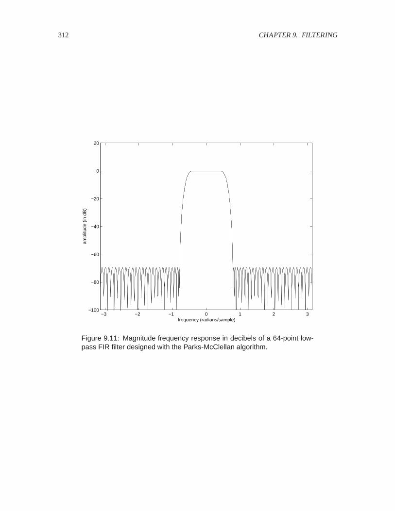
312 CHAPTER 9. FILTERING
−3 −2 −1 0 1 2 3−100
−80
−60
−40
−20
0
20
frequency (radians/sample)
ampl
itude
(in
dB
)
Figure 9.11: Magnitude frequency response in decibels of a 64-point low-pass FIR filter designed with the Parks-McClellan algorithm.
9.4. FINITE IMPULSE RESPONSE (FIR) FILTERS 313
Probing further: Decibels
The term “decibel” is literally one tenth of a bel, which is named after AlexanderGraham Bell. This unit of measure was originally developed by telephone engi-neers at Bell Telephone Labs to designate the ratio of the power of two signals.
Power is a measure of energy dissipation (work done) per unit time. It is measuredin watts for electronic systems. One bel is defined to be a factor of 10 in power.Thus, a 1000 watt hair dryer dissipates 1 bel, or 10 dB, more power than a 100 wattlight bulb. Let (� � watts be the power of the hair dryer and (� � be thepower of the light bulb. Then the ratio is
!�&���(��(�� � bel�
In decibels, this becomes
!�&���(��(�� � dB�
Comparing against (9.24) we notice a discrepancy. There, the multiplying factor is20, not 10. That is because the ratio in (9.24) is a ratio of amplitudes, not powers.In electronic circuits, if an amplitude represents the voltage across a resistor, thenthe power dissipated by the resistor is proportional to the squareof the amplitude.Let �� and �� be two such amplitudes. Then the ratio of their powers is
!�&��������
��� � � !�&����������
Hence the multiplying factor of 20 instead of 10.
A 3 dB power ratio amounts to a factor of 2 in power. In amplitudes, this is a ratioof��. The edge of the passband of a bandpass filter is often defined to be the
frequency at which the power drops to half, which is the frequency where the gainis 3 dB below the passband gain. The magnitude frequency response here is �
��
times the passband gain.
In audio technology, decibels are used to measure sound pressure. You might hearstatements like “a jet engine at 10 meters produces 120 dB of sound.” But decibelsmeasure power ratios, not absolute power, so what does such a statement mean?By convention, sound pressure is measured relative to a defined reference of 20micropascals, where a pascal is a pressure of 1 newton per square meter. For mostpeople, this is approximately the threshold of hearing at 1 kHz. Thus, a sound at 0dB is barely audible. A sound at 10 dB has 10 times the power. A sound at 100 dBhas �� times the power. You would not be surprised to learn, therefore, that thejet engine cited above would probably make you deaf without ear protection.

314 CHAPTER 9. FILTERING
9.5 Infinite impulse response (IIR) filters
The equation for an FIR filter (9.22) is a difference equation relating the output at index � to theinputs at indices � � 1 � through �. A more general form of this difference equation includesmore indices of the output,
� � Integers� ���� �1������
����'���'� ��������
����'���'� (9.25)
where 1 and 3 are positive integers, and ��'� and ��'� are filter coefficients, which are usuallyreal valued. If all the � coefficients are zero, then this reduces to an FIR filter with impulse response� � �. However, if any � coefficient is non-zero, then the impulse response of this filter will nevercompletely die out, since the output keeps getting recycled to affect future outputs. Such a filter iscalled an infinite impulse response or IIR filter, or sometimes a recursive filter.
Example 9.16: Consider a causal LTI system defined by the difference equation
� � Integers� ���� � ���� � ������ ��
We can find the impulse response by letting � � Æ, the Kronecker delta function. Sincethe system is causal, we know that ���� � for � ) (see page 304). Thus,
���� � if � )
��� �
��� � ��
���� � ���
���� � ���
Noticing the pattern, we conclude that
���� � �����0����
where 0 is the unit step, seen before in (2.15),
0��� �
� if � � otherwise
(9.26)
The output � and the magnitude of the frequency response (in dB) are plotted in figure9.12. Notice that this filter has about 20 dB of gain at DC, dropping to about -6 dB at� radians/sample.
9.5.1 Designing IIR filters
Designing IIR filters amounts to choosing the � and � coefficients for (9.25). As with FIR filters,how to choose these coefficients is a well-studied subject, and the results of this study are (for the
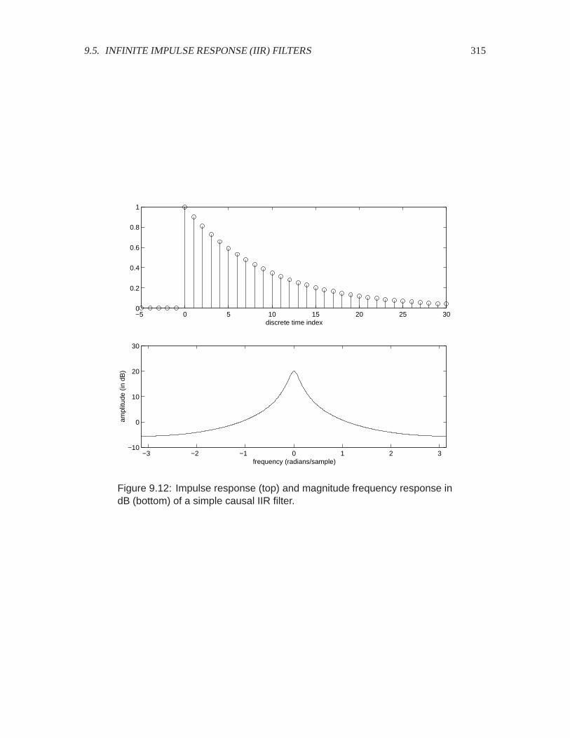
9.5. INFINITE IMPULSE RESPONSE (IIR) FILTERS 315
−5 0 5 10 15 20 25 300
0.2
0.4
0.6
0.8
1
discrete time index
−3 −2 −1 0 1 2 3−10
0
10
20
30
frequency (radians/sample)
ampl
itude
(in
dB
)
Figure 9.12: Impulse response (top) and magnitude frequency response indB (bottom) of a simple causal IIR filter.
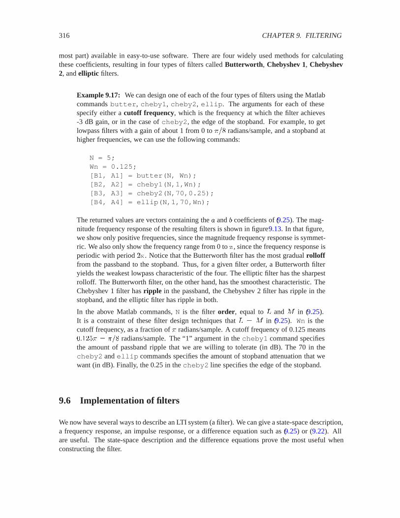
316 CHAPTER 9. FILTERING
most part) available in easy-to-use software. There are four widely used methods for calculatingthese coefficients, resulting in four types of filters called Butterworth, Chebyshev 1, Chebyshev2, and elliptic filters.
Example 9.17: We can design one of each of the four types of filters using the Matlabcommands butter, cheby1, cheby2, ellip. The arguments for each of thesespecify either a cutoff frequency, which is the frequency at which the filter achieves-3 dB gain, or in the case of cheby2, the edge of the stopband. For example, to getlowpass filters with a gain of about 1 from 0 to ��� radians/sample, and a stopband athigher frequencies, we can use the following commands:
N = 5;Wn = 0.125;[B1, A1] = butter(N, Wn);[B2, A2] = cheby1(N,1,Wn);[B3, A3] = cheby2(N,70,0.25);[B4, A4] = ellip(N,1,70,Wn);
The returned values are vectors containing the � and � coefficients of (9.25). The mag-nitude frequency response of the resulting filters is shown in figure9.13. In that figure,we show only positive frequencies, since the magnitude frequency response is symmet-ric. We also only show the frequency range from 0 to �, since the frequency response isperiodic with period ��. Notice that the Butterworth filter has the most gradual rollofffrom the passband to the stopband. Thus, for a given filter order, a Butterworth filteryields the weakest lowpass characteristic of the four. The elliptic filter has the sharpestrolloff. The Butterworth filter, on the other hand, has the smoothest characteristic. TheChebyshev 1 filter has ripple in the passband, the Chebyshev 2 filter has ripple in thestopband, and the elliptic filter has ripple in both.
In the above Matlab commands, N is the filter order, equal to 1 and 3 in (9.25).It is a constraint of these filter design techniques that 1 � 3 in (9.25). Wn is thecutoff frequency, as a fraction of � radians/sample. A cutoff frequency of 0.125 means���� � ��� radians/sample. The “1” argument in the cheby1 command specifiesthe amount of passband ripple that we are willing to tolerate (in dB). The 70 in thecheby2 and ellip commands specifies the amount of stopband attenuation that wewant (in dB). Finally, the 0.25 in the cheby2 line specifies the edge of the stopband.
9.6 Implementation of filters
We now have several ways to describe an LTI system (a filter). We can give a state-space description,a frequency response, an impulse response, or a difference equation such as (9.25) or (9.22). Allare useful. The state-space description and the difference equations prove the most useful whenconstructing the filter.
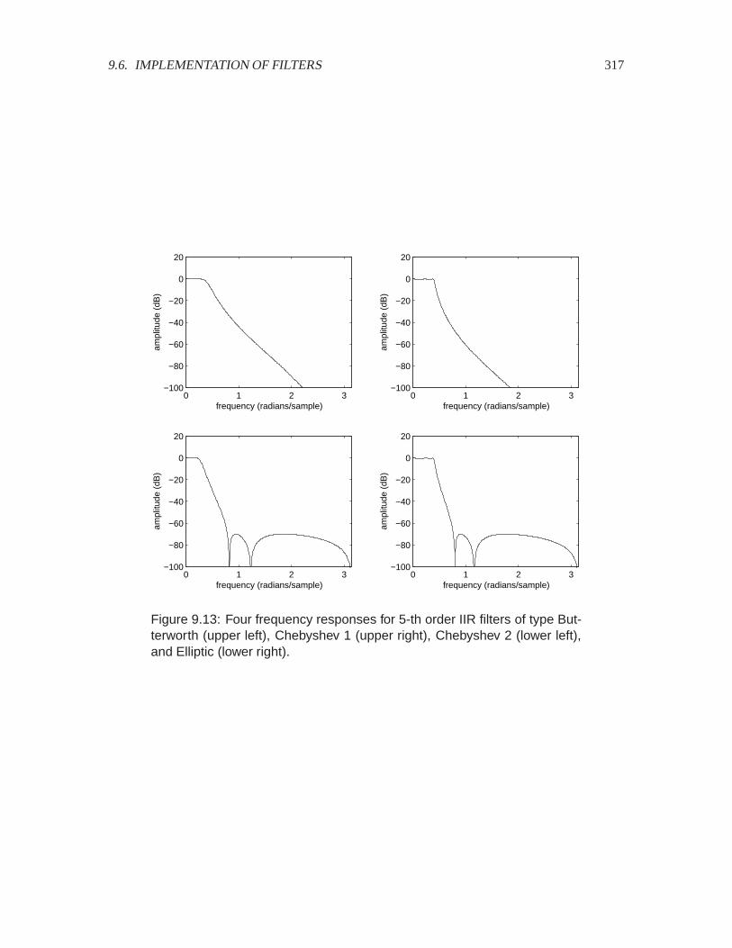
9.6. IMPLEMENTATION OF FILTERS 317
0 1 2 3−100
−80
−60
−40
−20
0
20
frequency (radians/sample)
ampl
itude
(dB
)
0 1 2 3−100
−80
−60
−40
−20
0
20
frequency (radians/sample)
ampl
itude
(dB
)0 1 2 3
−100
−80
−60
−40
−20
0
20
frequency (radians/sample)
ampl
itude
(dB
)
0 1 2 3−100
−80
−60
−40
−20
0
20
frequency (radians/sample)
ampl
itude
(dB
)
Figure 9.13: Four frequency responses for 5-th order IIR filters of type But-terworth (upper left), Chebyshev 1 (upper right), Chebyshev 2 (lower left),and Elliptic (lower right).
318 CHAPTER 9. FILTERING
A realization of a filter in hardware or software is called an implementation. Do not confuse filterdesign with filter implementation. The term “filter design” is used in the community to refer tothe choice of frequency response, impulse response, or coefficients for a difference equation, not tohow the frequency response is implemented in hardware or software. In this section, we talk aboutimplementation.
The output � of an FIR filter with impulse response � and input � is given by (9.22). The output ofan IIR filter with coefficients � and � is given by (9.25). Each of these difference equations definesa procedure for calculating the output given the input. We discuss various ways of implementingthese procedures.
9.6.1 Matlab implementation
If � is finite, and we can interpret it as an infinite signal that is zero outside the specified range.Then we can compute the output of an FIR filter using Matlab’s conv function, and the output ofan IIR filter using filter.
Example 9.18: Consider an FIR filter with an impulse response of length 1. If x is avector containing the � values of the input, and h is a vector containing the 1 valuesof the impulse response, then
y = conv(x, h);
yields a vector containing 1� � � values of the output.
For IIR examples using filter, see lab C.10. This strategy, of course, only works for finite inputdata, since Matlab requires that the input be available in a finite vector.
Discrete-time filters can be implemented using standard programming languages and using assem-bly languages on specialized processors (see boxes). These implementations do not have the limi-tation that the input be finite.
9.6.2 Signal flow graphs
We can describe the computations in a discrete-time filter using a block diagram with three visualelements, a unit delay, a multiplier, and an adder. In the convolution sum for an FIR filter,
���� �1������
��'�����'��
notice that at each � we need access to ����, �����, ������, , ����1��. We can maintainthis set of values by cascading a set of unit delay elements to form a delay line, as shown in figure9.14.

9.6. IMPLEMENTATION OF FILTERS 319
Probing further: Java implementation of an FIR filter
The following Java class implements an FIR filter:
1 class FIR {2 private int length;3 private double[] delayLine;4 private double[] impResp;5 private int count = 0;6 FIR(double[] coefs) {7 length = coefs.length;8 impResp = coefs;9 delayLine = new double[length];10 }11 double getOutputSample(double inputSample) {12 delayLine[count] = inputSample;13 double result = 0.0;14 int index = count;15 for (int i=0; i<length; i++) {16 result += impResp[i] * delayLine[index--];17 if (index < 0) index = length-1;18 }19 if (++count >= length) count = 0;20 return result;21 }22 }
A class in Java (and in any object-oriented language) has both data members andmethods. The methods are procedures that operate on the data members, and mayor may not take arguments or return values. In this case, there are two procedures,“FIR” and “getOutputSample.” The first, lines 6-10, is a constructor, which is aprocedure that is called to create an FIR filter. It takes one argument, an array ofdouble-precision floating-point numbers that specify the impulse response of thefilter. The second, lines 11-22, takes a new input sample value as an argumentand returns a new output sample. It also updates the delay line using a strategycalled circular buffering. That is, the “count” member is used to keep track ofwhere each new input sample should go. It gets incremented (line 19) each timethe getOutputSample() method is called. When it exceeds the length of thebuffer, it gets reset to zero. Thus, at all times, it contains the 1 most recentlyreceived input data samples. The most recent one is at index count in the buffer.The second most recent is at count - 1, or if that is negative, at length -1. Line 17 makes sure that the variable index remains within the confines of thebuffer as we iterate through the loop.

320 CHAPTER 9. FILTERING
Probing further: Programmable DSP implementation of an FIR filter
The following section of code is the assembly language for a programmable DSP,which is a specialized microprocessor designed to implement signal processingfunctions efficiently in embedded systems (such as cellular telephones, digital cord-less telephones, digital audio systems, etc.). This particular code is for the MotorolaDSP56000 family of processors.
1 fir movep x:input,x:(r0)2 clr a x:(r0)-,x0 y:(r4)+,y03 rep m04 mac x0,y0,a x:(r0)-,x0 y:(r4)+,y05 macr x0,y0,a (r0)+6 movep a,x:output7 jmp fir
This processor has two memory banks called x and y. The code assumes that eachinput sample can be successively read from a memory location called input, andthat the impulse response is stored in y memory beginning at an address stored inregister r4. Moreover, it assumes that register r0 contains the address of a sectionof x memory to use for storing input samples (the delay line), and that this registerhas been set up to perform modulo addressing. Modulo addressing means that ifit increments or decrements beyond the range of its buffer, then the address wrapsaround to the other end of the buffer. Finally, it assumes that the register m0 con-tains an integer specifying the number of samples in the impulse response minusone.
The key line (the one that does most of the work) is line 4. It follows a repinstruction, which causes that one line to be repeatedly executed the number oftimes specified by register m0. Line 4 multiplies the data in register x0 by thatin y0 and adds the result to a (the accumulator). Such an operation is called amultiply and accumulate or mac operation. At the same time, it loads x0 with aninput sample from the delay line, in x memory at a location given by r0. It alsoloads register y0 with a sample from the impulse response, stored in y memory ata location given by r4. At the same time, it increments r0 and decrements r4. Thisone-line instruction, which carries out several operations in parallel, is obviouslyhighly tuned to FIR filtering. Indeed, FIR filtering is a major function of processorsof this type.
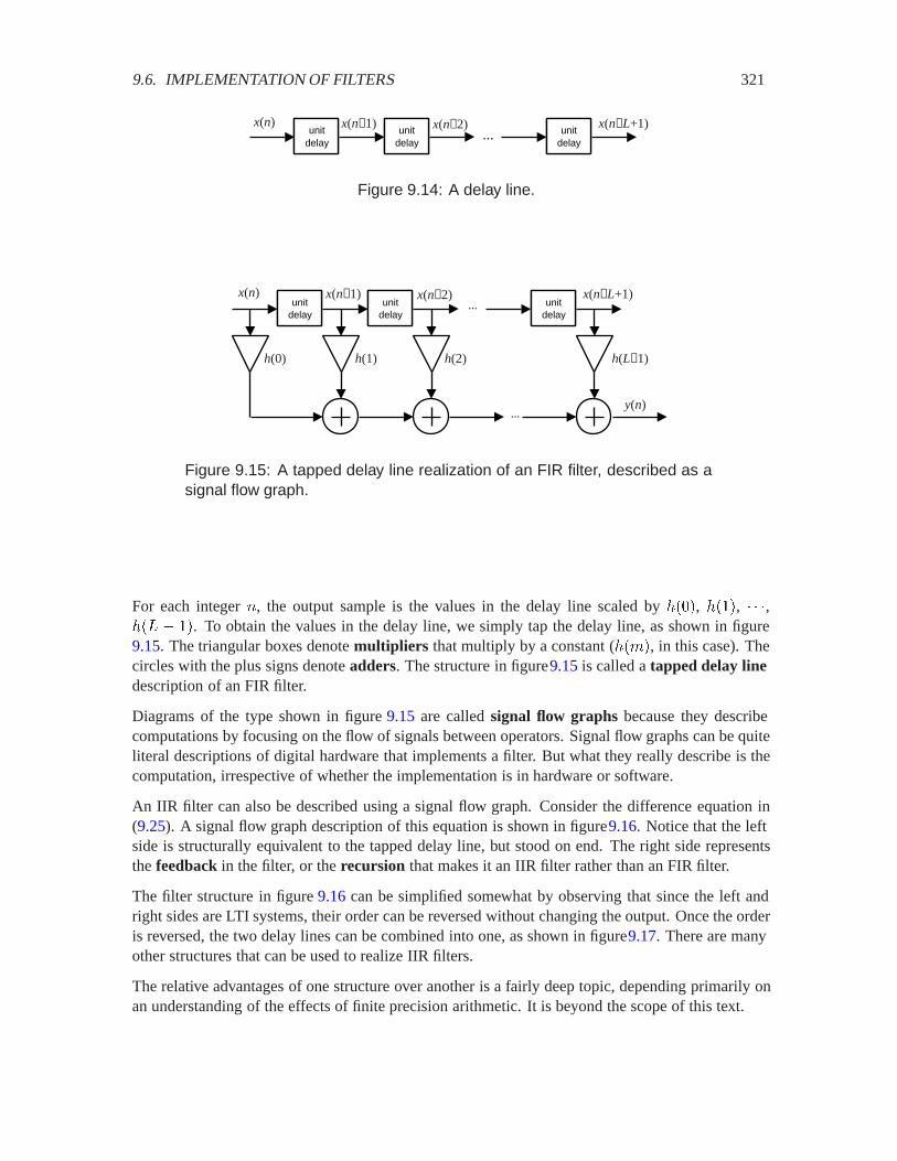
9.6. IMPLEMENTATION OF FILTERS 321
unitdelay
unitdelay
unitdelay
x(n) x(n−1) x(n−2) x(n−L+1)...
Figure 9.14: A delay line.
unitdelay
unitdelay
unitdelay
x(n) x(n−1) x(n−2) x(n−L+1)
h(L−1)h(2)h(1)h(0)
y(n)
...
...
Figure 9.15: A tapped delay line realization of an FIR filter, described as asignal flow graph.
For each integer �, the output sample is the values in the delay line scaled by ���, ���, ,��1 � �. To obtain the values in the delay line, we simply tap the delay line, as shown in figure9.15. The triangular boxes denote multipliers that multiply by a constant (��'�, in this case). Thecircles with the plus signs denote adders. The structure in figure9.15 is called a tapped delay linedescription of an FIR filter.
Diagrams of the type shown in figure 9.15 are called signal flow graphs because they describecomputations by focusing on the flow of signals between operators. Signal flow graphs can be quiteliteral descriptions of digital hardware that implements a filter. But what they really describe is thecomputation, irrespective of whether the implementation is in hardware or software.
An IIR filter can also be described using a signal flow graph. Consider the difference equation in(9.25). A signal flow graph description of this equation is shown in figure9.16. Notice that the leftside is structurally equivalent to the tapped delay line, but stood on end. The right side representsthe feedback in the filter, or the recursion that makes it an IIR filter rather than an FIR filter.
The filter structure in figure 9.16 can be simplified somewhat by observing that since the left andright sides are LTI systems, their order can be reversed without changing the output. Once the orderis reversed, the two delay lines can be combined into one, as shown in figure9.17. There are manyother structures that can be used to realize IIR filters.
The relative advantages of one structure over another is a fairly deep topic, depending primarily onan understanding of the effects of finite precision arithmetic. It is beyond the scope of this text.

322 CHAPTER 9. FILTERING
x(n)
x(n−1)
x(n−2)
b(L−1)
b(2)
b(1)
b(0) y(n)
unitdelay
unitdelay
...
unitdelay
y(n−1)
y(n−2)
a(M−1)
a(2)
a(1)unit
delay
unitdelay
...
unitdelay
y(n−M+1)x(n−L+1)
......
Figure 9.16: A signal flow graph describing an IIR filter. This is called adirect form 1 filter structure.
9.7 Summary
The output of an LTI system does not contain any frequencies that are not also present in the input.Because of this property, LTI systems are often called filters. This chapter considers how filtersmight be implemented. The convolution sum (for discrete-time systems) and convolution integral(for continuous-time systems) give descriptions of how to calculate an output given an input sig-nal. This description highlights the usefulness of the response that a system has to an idealizedimpulse, because the output is given by the convolution of the input and the impulse response. Thefrequency response, moreover, is shown to be Fourier transform of the impulse response, where theFourier transform is a generalization of the Fourier series considered in previous chapters. Fouriertransforms are considered in much more depth in the next chapter.
This chapter also considers the design of filters, by which we mean the selection of a suitable fre-quency response. Engineers are, as usual, forced to compromise to get an acceptable response at anacceptable computational cost. The response is assessed by considering how effectively it performsthe desired filtering operation, and the cost is assessed by considering the arithmetic calculation thatmust be realized to implement the filter. The chapter closes with a discussion of alternative ways ofrealizing the arithmetic calculation.
Exercises
Each problem is annotated with the letter E, T, C which stands for exercise, requires some thought,requires some conceptualization. Problems labeled E are usually mechanical, those labeled T re-quire a plan of attack, those labeled C usually have more than one defensible answer.
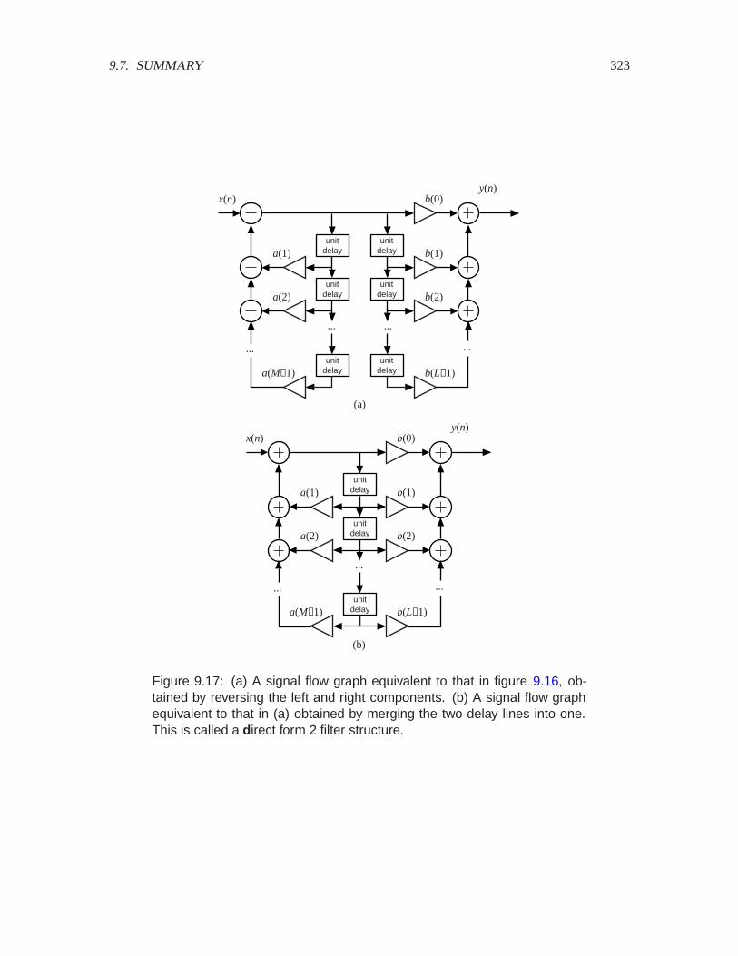
9.7. SUMMARY 323
x(n)
b(L−1)
b(2)
b(1)
b(0)y(n)
unitdelay
unitdelay
...
unitdelaya(M−1)
a(2)
a(1)unit
delay
unitdelay
...
unitdelay
x(n)
b(L−1)
b(2)
b(1)
b(0)y(n)
a(M−1)
a(2)
a(1)unit
delay
unitdelay
...
unitdelay
(a)
(b)
... ...
......
Figure 9.17: (a) A signal flow graph equivalent to that in figure 9.16, ob-tained by reversing the left and right components. (b) A signal flow graphequivalent to that in (a) obtained by merging the two delay lines into one.This is called a direct form 2 filter structure.

324 CHAPTER 9. FILTERING
1. E Consider an LTI discrete-time system Filter with impulse response
���� ���
���
��� 6��
where Æ is the Kronecker delta function.
(a) Sketch ����.
(b) Suppose the input signal �� Integers� Realsis such that � � Integers, ���� ��������, where � � ��� radians/sample. Give a simple expression for � � Filter���.
(c) Give the value of ;��� for � � ���, where ; is the frequency response.
2. E Consider the continuous-time moving average system ., whose impulse response is shownin figure 9.3. Find its frequency response. The following fact from calculus may be useful:
���
���!�� � ��� � ���
for real � and � and complex !. Use Matlab to plot the magnitude of this frequency responseover the range -5 Hz to 5 Hz. Note the symmetry of the magnitude response, as required by(9.21).
3. E Consider a continuous-time LTI system with impulse response given by
� Reals� ��� � � � � � � � ���
where Æ is the Dirac delta function.
(a) Find a simple equation relating the input � and output � of this system.
(b) Find the frequency response of this system.
(c) Use Matlab to plot the magnitude frequency response of this system in the range -5 to 5Hz.
4. E Consider a discrete-time LTI system with impulse response � given by
� � Integers� ���� � ��� � ���� �
(a) Plot the impulse response.
(b) Find and sketch the output when the input is 0, the unit step, given by (9.26).
(c) Find and sketch the output when the input is a ramp,
���� �
�� if � � otherwise
(d) Find the frequency response.
(e) Show that the frequency response is periodic with period ��.
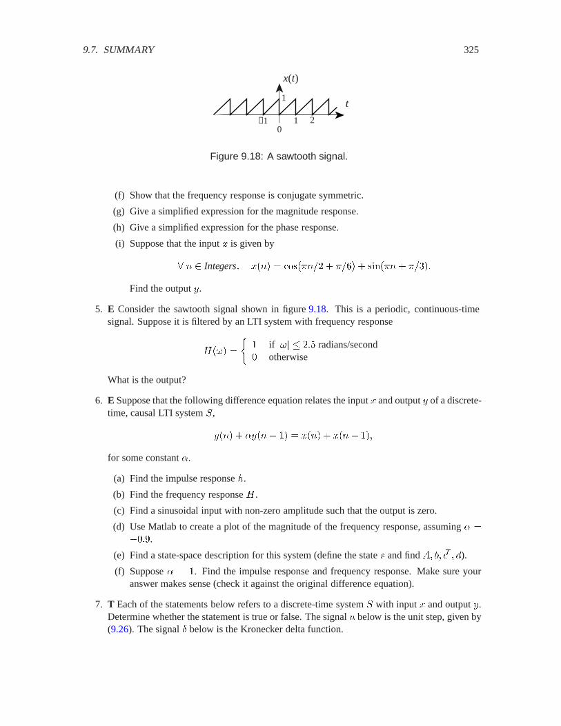
9.7. SUMMARY 325
x(t)
t1
1 20
−1
Figure 9.18: A sawtooth signal.
(f) Show that the frequency response is conjugate symmetric.
(g) Give a simplified expression for the magnitude response.
(h) Give a simplified expression for the phase response.
(i) Suppose that the input � is given by
� � Integers� ���� � �������� � �� � � ������� �����
Find the output �.
5. E Consider the sawtooth signal shown in figure 9.18. This is a periodic, continuous-timesignal. Suppose it is filtered by an LTI system with frequency response
;��� �
� if ��� � ��� radians/second otherwise
What is the output?
6. E Suppose that the following difference equation relates the input � and output � of a discrete-time, causal LTI system .,
���� � *���� � � ���� � ���� ��
for some constant *.
(a) Find the impulse response �.
(b) Find the frequency response ; .
(c) Find a sinusoidal input with non-zero amplitude such that the output is zero.
(d) Use Matlab to create a plot of the magnitude of the frequency response, assuming * ����.
(e) Find a state-space description for this system (define the state � and find �� �� !� � �).
(f) Suppose * � . Find the impulse response and frequency response. Make sure youranswer makes sense (check it against the original difference equation).
7. T Each of the statements below refers to a discrete-time system . with input � and output �.Determine whether the statement is true or false. The signal 0 below is the unit step, given by(9.26). The signal Æ below is the Kronecker delta function.
326 CHAPTER 9. FILTERING
(a) Suppose you know that if � is a sinusoid then � is a sinusoid. Then you can concludethat . is LTI.
(b) Suppose you know that . is LTI, and that if ���� � ���������, then ���� � � ���������.Then you have enough information to determine the frequency response.
(c) Suppose you know that . is LTI, and that if ���� � ���, then
���� � �����0����
Then you have enough information to determine the frequency response.
(d) Suppose you know that . is LTI, and that if ���� � 0���, then ���� � �����0���.Then you have enough information to determine the frequency response.
(e) Suppose you know that . is causal, and that input ���� � ��� produces output ���� ���������, and input ����� � ����� produces output ����� � ������������.Then you can conclude that . is not LTI.
(f) Suppose you know that . is causal, and that if ���� � ��� � �� � �� then ���� ���� � ��� � � ��� � �� � ��� ��. Then you can conclude that . is not LTI.
8. T Consider the continuous-time systems .� given by, � Reals,
�.������� � ��� ���
�.������� � ��� ���
�.������� � ���� ��
�.������ � ���� ��
�.������� � �����
�.������� � �����
(a) Which of these systems is linear?
(b) Which of these systems is time invariant?
(c) Which of these systems is causal?
9. T Consider an LTI discrete-time system Filter with impulse response
� � Integers� ���� � ��� � ��� ���
where Æ is the Kronecker delta function.
(a) Sketch �.
(b) Find the output when the input is 0, the unit step, given by (9.26).
(c) Find the output when the input is a ramp,
���� �
�� if � � otherwise

9.7. SUMMARY 327
(d) Suppose the input signal � is such that
� � Integers� ���� � ��������
where � � ��� radians/sample. Give a simple expression for � � Filter���.
(e) Give an expression for ;��� that is valid for all � , where ; is the frequency response.
(f) Sketch the magnitude of the frequency response. Can you explain your answer in part(b)?
(g) Is there any other frequency at which a sinusoidal input with a non-zero amplitude willyield an output that is zero?
10. T Consider an LTI discrete-time system Filter with impulse response
���� � ���� ��� �
where Æ is the Kronecker delta function.
(a) Sketch ����.
(b) Suppose the input signal �� Integers� Realsis such that � � Integers, ���� � .Give a simple expression for � � Filter���.
(c) Give an expression for ;��� that is valid for all � , where ; is the frequency response.
(d) Sketch the magnitude of the frequency response. Can you explain your answer in part(b)?
11. T Consider a discrete-time LTI system with impulse response � given by
� � Integers� ���� � ��� ��� � ��� ���
And consider the periodic discrete-time signal given by
� � Integers� ���� � � � ��������� � ��������
(a) Is the system causal?
(b) Find the frequency response of the system. Check that your answer is periodic withperiod ��.
(c) For the given signal �, find the fundamental frequency �� and the Fourier series coeffi-cients �� in the Fourier series expansion,
���� ���
����
���������
Give the units of the fundamental frequency.
(d) Assuming the input to the system is � as given, find the output.

328 CHAPTER 9. FILTERING
12. T Consider a continuous-time LTI system .. Suppose that when the input is the continuous-time unit step, given by
0�� �
�� � � )
(9.27)
then the output � � .�0� is given by
��� �
�� � � � otherwise
This output � is called the step response because it is the response to a unit step.
(a) Express � in terms of sums and differences of 0 and ���0�, where �� is the delayoperator.
(b) Give a signal flow graph that produces this result � � .�0� when the input is 0. Note:We know that if two LTI systems have the same impulse response, then they are thesame system. It is a fact, albeit a non-trivial one to demonstrate, that if two LTI systemshave the same step response, then they are also the same system. Thus, your signal flowgraph implements ..
(c) Use your signal flow graph to determine what the output �� of . is when the input is
��� �
�� � � � otherwise
Plot your answer.
(d) What is the frequency response ;��� of .?
13. T Suppose a discrete-time LTI system . has impulse response
���� � 0������ �
���� if � � otherwise
where 0 is the unit step function (9.26).
(a) What is the step response of this system? The step response is defined to be the outputwhen the input is the unit step. Hint: The identity (9.23) might be helpful.
(b) What is the frequency response? Plot the magnitude and phase response (you may useMatlab, or do it by hand). Hint: The following variant of the identity (9.23) might beuseful. If ��� ) ,
�����
�� �
� ��
This follows immediately from (9.23) by letting 1 go to infinity.
(c) Suppose . is put in cascade with another identical system. What is the frequency re-sponse of the cascade composition?
(d) Suppose . is arranged in a feedback composition as shown in figure9.19. What is thefrequency response of the feedback composition?

9.7. SUMMARY 329
x(n) y(n)S+−
Figure 9.19: Feedback composition.

330 CHAPTER 9. FILTERING

Chapter 10
The Four Fourier Transforms
In chapter 7 we saw that the Fourier series describes a periodic signal as a sum of complex expo-nentials. In chapter 8 we saw that if the input to an LTI system is a sum of complex exponentials,then the frequency response of the LTI system describes its response to each of the component ex-ponentials. Thus we can calculate the system response to any periodic input signal by combiningthe responses to the individual components.
In chapter 9 we saw that the response of the LTI system to any input signal can also be obtainedas the convolution of the input signal and the impulse response. The impulse response and thefrequency response give us the same information about the system, but in different forms. Theimpulse response and the frequency response are related by the Fourier transform, where in chapter9we saw both discrete time and continuous time versions.
In this chapter, we will see that for discrete-time systems, the frequency response can be described asa sum of weighted complex exponentials (the DTFT), where the weights turn out to be the impulseresponse samples. We will see that the impulse response is, in fact, a Fourier series representation ofthe frequency response, with the roles of time and frequency reversed from the uses of the Fourierseries that we have seen so far.
This reappearance of the Fourier series is not a coincidence. In this chapter, we explore this patternby showing that the Fourier series is a special case of a family of representations of signals that arecollectively called Fourier transforms. The Fourier series applies specifically to continuous-time,periodic signals. The discrete Fourier series applies to discrete-time, periodic signals. We completethe story with the continuous-time Fourier transform (CTFT), which applies to continuous-timesignals that are not periodic, and the discrete-time Fourier transform (DTFT), which applies todiscrete-time signals that are not periodic.
331
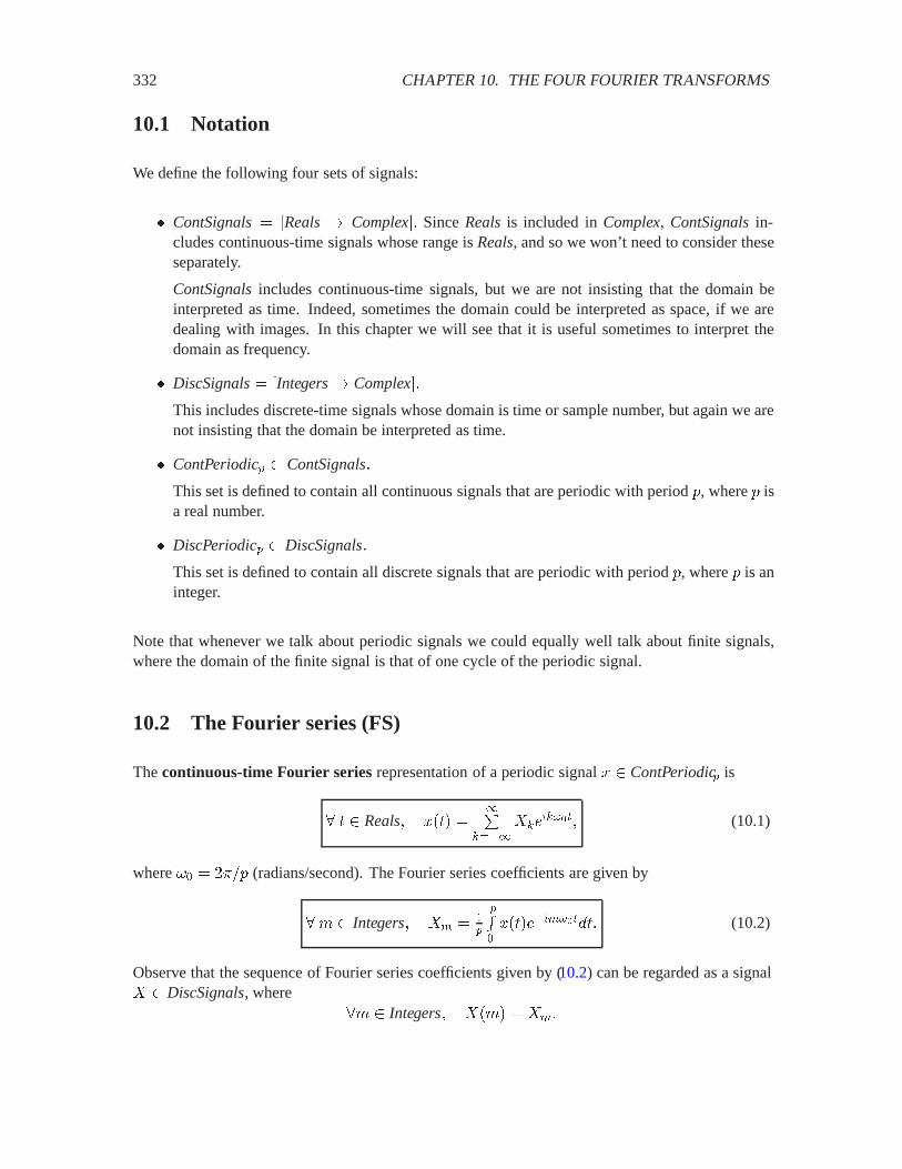
332 CHAPTER 10. THE FOUR FOURIER TRANSFORMS
10.1 Notation
We define the following four sets of signals:
� ContSignals� �Reals� Complex�� Since Realsis included in Complex, ContSignalsin-cludes continuous-time signals whose range is Reals, and so we won’t need to consider theseseparately.
ContSignalsincludes continuous-time signals, but we are not insisting that the domain beinterpreted as time. Indeed, sometimes the domain could be interpreted as space, if we aredealing with images. In this chapter we will see that it is useful sometimes to interpret thedomain as frequency.
� DiscSignals� �Integers� Complex��
This includes discrete-time signals whose domain is time or sample number, but again we arenot insisting that the domain be interpreted as time.
� ContPeriodic# � ContSignals�
This set is defined to contain all continuous signals that are periodic with period (, where ( isa real number.
� DiscPeriodic# � DiscSignals�
This set is defined to contain all discrete signals that are periodic with period (, where ( is aninteger.
Note that whenever we talk about periodic signals we could equally well talk about finite signals,where the domain of the finite signal is that of one cycle of the periodic signal.
10.2 The Fourier series (FS)
The continuous-time Fourier series representation of a periodic signal � ContPeriodic# is
� Reals� ��� ���
�������
������ (10.1)
where �� � ���( (radians/second). The Fourier series coefficients are given by
�' Integers� �� � �#
#"������������� (10.2)
Observe that the sequence of Fourier series coefficients given by (10.2) can be regarded as a signal� DiscSignals, where
�' Integers� ��'� � ���
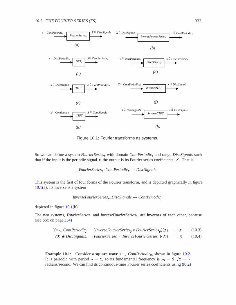
10.2. THE FOURIER SERIES (FS) 333
InverseFourierSeriesp
X ∈ DiscSignals x ∈ ContPeriodicp
(a)
DFTp
X ∈ DiscPeriodicpx ∈ DiscPeriodicp
(b)
InverseDFTpX ∈ DiscPeriodicp x ∈ DiscPeriodicp
(c)
DTFTX ∈ ContPeriodic2πx ∈ DiscSignals
(d)
InverseDTFTX ∈ ContPeriodic2π x ∈ DiscSignals
(e)
CTFTX ∈ ContSignalsx ∈ ContSignals
(f)
InverseCTFTX ∈ ContSignals x ∈ ContSignals
(g)
FourierSeriesp
X ∈ DiscSignalsx ∈ ContPeriodicp
(h)
Figure 10.1: Fourier transforms as systems.
So we can define a system FourierSeries# with domain ContPeriodic# and range DiscSignalssuchthat if the input is the periodic signal �, the output is its Fourier series coefficients, � . That is,
FourierSeries#�ContPeriodic# � DiscSignals�
This system is the first of four forms of the Fourier transform, and is depicted graphically in figure10.1(a). Its inverse is a system
InverseFourierSeries#�DiscSignals� ContPeriodic#�
depicted in figure 10.1(b).
The two systems, FourierSeries# and InverseFourierSeries#, are inverses of each other, because(see box on page 334)
�� ContPeriodic#� �InverseFourierSeries# Æ FourierSeries#���� � � (10.3)
�� DiscSignals� �FourierSeries# Æ InverseFourierSeries#���� � � (10.4)
Example 10.1: Consider a square wave � ContPeriodic�, shown in figure 10.2.It is periodic with period ( � �, so its fundamental frequency is �� � ���� � �radians/second. We can find its continuous-time Fourier series coefficients using (10.2)
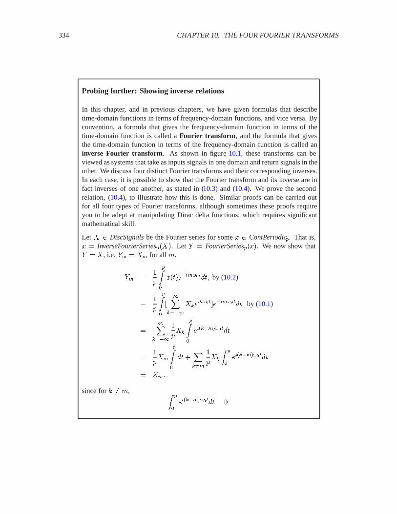
334 CHAPTER 10. THE FOUR FOURIER TRANSFORMS
Probing further: Showing inverse relations
In this chapter, and in previous chapters, we have given formulas that describetime-domain functions in terms of frequency-domain functions, and vice versa. Byconvention, a formula that gives the frequency-domain function in terms of thetime-domain function is called a Fourier transform, and the formula that givesthe time-domain function in terms of the frequency-domain function is called aninverse Fourier transform. As shown in figure 10.1, these transforms can beviewed as systems that take as inputs signals in one domain and return signals in theother. We discuss four distinct Fourier transforms and their corresponding inverses.In each case, it is possible to show that the Fourier transform and its inverse are infact inverses of one another, as stated in (10.3) and (10.4). We prove the secondrelation, (10.4), to illustrate how this is done. Similar proofs can be carried outfor all four types of Fourier transforms, although sometimes these proofs requireyou to be adept at manipulating Dirac delta functions, which requires significantmathematical skill.
Let � DiscSignalsbe the Fourier series for some � ContPeriodic#. That is,� � InverseFourierSeries#���. Let $ � FourierSeries#���. We now show that$ � � , i.e. $� � �� for all '.
$� �
(
#��
������������ by (10.2)
�
(
#��
���
����
������������������ by (10.1)
���
����
(��
#��
�� ��������
�
(��
#��
���� ���
(��
� #
��� ��������
� ���
since for 6 �� ', � #
��� �������� � �

10.2. THE FOURIER SERIES (FS) 335
x(t)
t1
1 2
Figure 10.2: A square wave.
|Xm|
m
1/21/π
1/3π1/5π 1/7π
Figure 10.3: Magnitude of the Fourier series coefficients of a square wave.
as follows,
�� �
�
���
�������)��
�
�
���
����)���
Notice that when ' � , this integral is easy to evaluate because �� � , so
�� � ���
The following fact from calculus will help us solve the integral when ' �� ,
���
���! �� � ��� � ��� (10.5)
for real � and � and complex !. Letting ! � �&'�, the integral becomes
�� �
�!
���
���! �
��
�&'������) � ���
�&
�'������) � �
336 CHAPTER 10. THE FOUR FOURIER TRANSFORMS
where the last step follows from multiplying top and bottom by &, observing that &� ��, and observing that �� � . Notice that
����) �
� if ' is even� if ' is odd
Thus, when ' �� ,
�� �
� if ' is even�&�'� if ' is odd
The magnitude of these Fourier series coefficients is plotted in figure10.3. Notice thatthe magnitudes of the coefficients decay rather slowly as ' gets large (they decay as1/'). This accounts for the persistent overshoot (Gibbs phenomenon) seen in figure7.6. Finite Fourier series approximations of this periodic square wave are not particu-larly good because the size of the Fourier series coefficients decays slowly.
Other examples of Fourier series coefficients for various signals are given in table10.1.
10.3 The discrete Fourier transform (DFT)
The discrete-time Fourier series (DFS) expansion for � DiscPeriodic# is (see (8.30))
� � Integers� ���� �#������
��������� (10.6)
where �� � ���( (radians/sample). The Fourier series coefficients can be found using the formula
� 6 Integers� �� �
(
#������
��'�������� � (10.7)
For historical reasons, the discrete Fourier transform (DFT) is the DFS with slightly differentscaling. It is defined by
� � Integers� ���� � �#
#������
� ���
������ (10.8)
� 6 Integers� ��� �
#������
��'�������� � (10.9)
Obviously, the DFT coefficients are related to the DFS coefficients by
� �� � (���
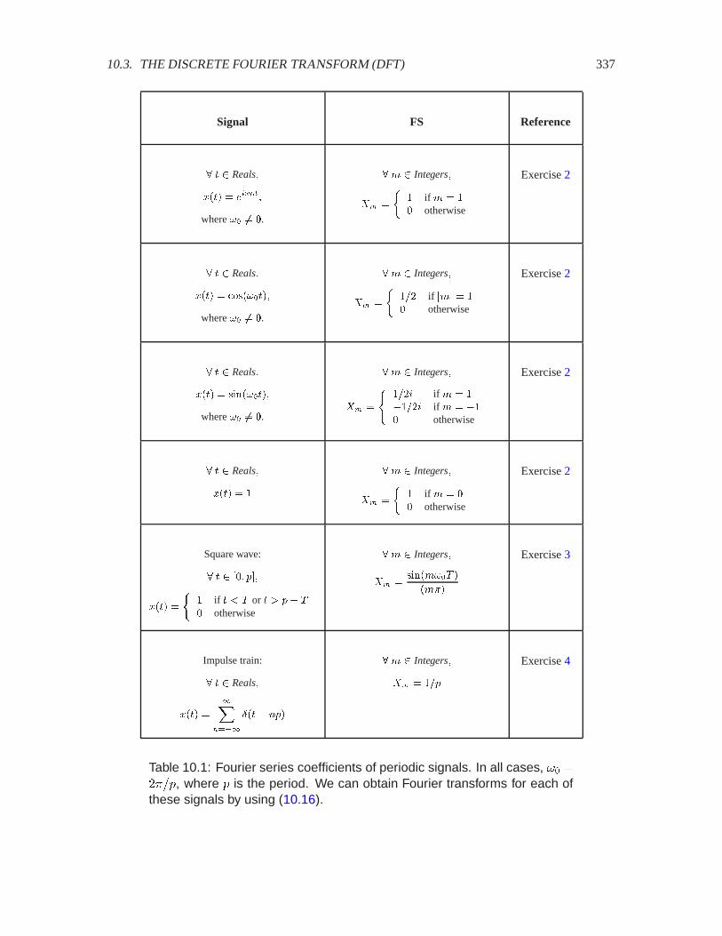
10.3. THE DISCRETE FOURIER TRANSFORM (DFT) 337
Signal FS Reference
� � � Reals�
���� � �����
where �� �� �.
� � � Integers�
�� �
�� if � � �� otherwise
Exercise 2
� � � Reals�
���� � ��������
where �� �� �.
� � � Integers�
�� �
���� if � � �� otherwise
Exercise 2
� � � Reals�
���� � ��������
where �� �� �.
� � � Integers�
�� �
����� if � � ������ if � � ��� otherwise
Exercise 2
� � � Reals�
���� � �
� � � Integers�
�� �
�� if � � �� otherwise
Exercise 2
Square wave:
� � � ��� ���
���� �
�� if � � � or � � �� �� otherwise
� � � Integers�
�� �������� �
����
Exercise 3
Impulse train:
� � � Reals�
���� �
���
��� ���
� � � Integers�
�� � ���
Exercise 4
Table 10.1: Fourier series coefficients of periodic signals. In all cases, �� ����(, where ( is the period. We can obtain Fourier transforms for each ofthese signals by using (10.16).

338 CHAPTER 10. THE FOUR FOURIER TRANSFORMS
This scaling is somewhat unfortunate, since it means that the DFT coefficients do not have the sameunits as the signal �, but the scaling is firmly established in the literature, so we stick to it. We omitthe prime when it is clear whether we are talking about the Fourier transform instead of the Fourierseries.
Observe that �� � DFT#��� is a discrete signal that is itself periodic with period (. To verify this,note that for any integer � and for all integers 6,
� ����# �
#������
��'����� ���#���
�#������
��'�������������#��
�#������
��'��������������)� since �� � ���(
�#������
��'��������
� � ���
Note that (10.9) looks like a discrete Fourier series expansion of the periodic function ��. That is,the periodic function is described as a sum of complex exponentials. The only substantial difference,comparing with (10.6), is the sign of the exponent. This sign difference can be easily removed with achange of variables. By doing so, you can discover that ���'� is the '-th Fourier series coefficientfor the function ��! The DFT is rather special, therefore, in that both the time and frequency domainrepresentations of a function are Fourier series, and both are periodic.
The DFT therefore is the function
DFT#�DiscPeriodic# � DiscPeriodic#�
given by (10.9). The inverse DFT is the function
InverseDFT#�DiscPeriodic# � DiscPeriodic#�
given by (10.8). As in (10.3), (10.4), DFT# and InverseDFT# are inverses of each other. This canbe verified using methods similar to those in the box on page 334. The DFT and its inverse arecomputed by systems that we can represent as shown in figure10.1(c) and (d).
The DFT is the most useful form of the Fourier transform for computation, because the system DFT#is easily implemented on a computer. Both summations (10.8) and (10.9) are finite. Moreover, thereis an algorithm called the fast Fourier transform (FFT) that calculates these summations with farfewer arithmetic operations than the most direct method. Moreover, because the sums are finite, theDFT always exists. There are no mathematical problems with convergence.
Example 10.2: Consider a discrete square wave � DiscPeriodic�, shown in figure10.4. It is periodic with period ( � �, so its fundamental frequency is �� � ���� �
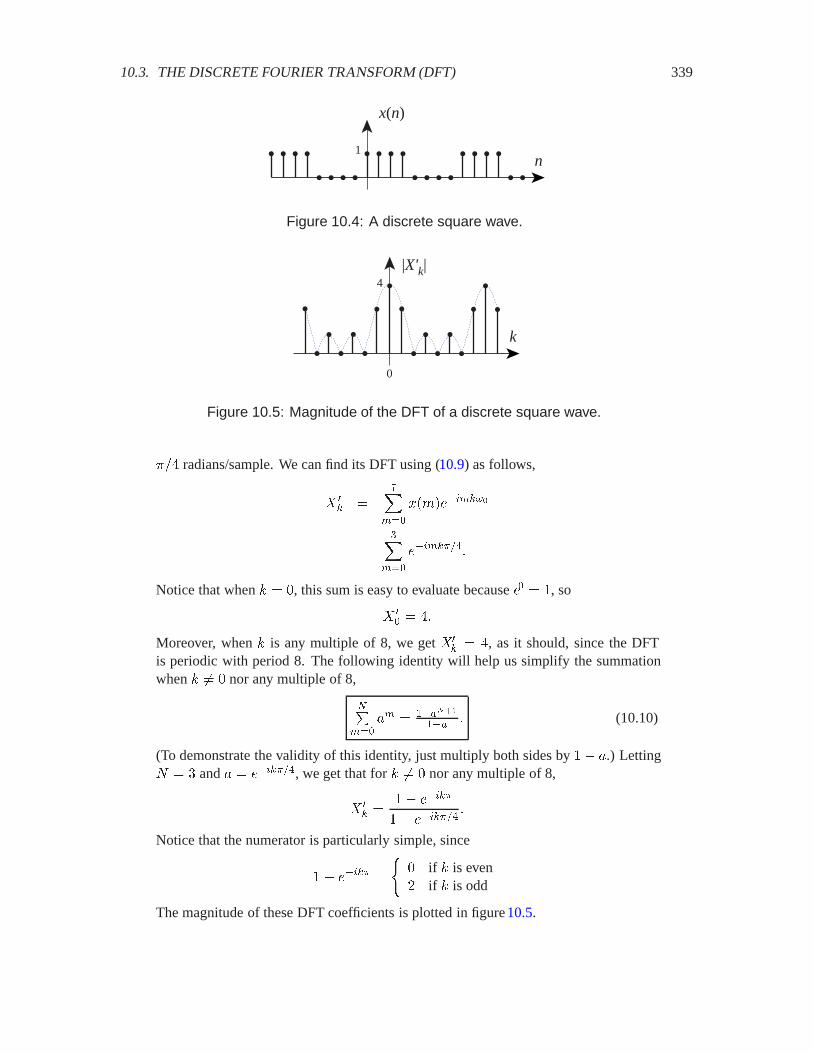
10.3. THE DISCRETE FOURIER TRANSFORM (DFT) 339
x(n)
n1
Figure 10.4: A discrete square wave.
|X'k|
k
4
0
Figure 10.5: Magnitude of the DFT of a discrete square wave.
��� radians/sample. We can find its DFT using (10.9) as follows,
� �� �
�����
��'��������
���
���
�����)��
Notice that when 6 � , this sum is easy to evaluate because �� � , so
� �� � ��
Moreover, when 6 is any multiple of 8, we get ��� � �, as it should, since the DFT
is periodic with period 8. The following identity will help us simplify the summationwhen 6 �� nor any multiple of 8,
�����
�� � ������
��� � (10.10)
(To demonstrate the validity of this identity, just multiply both sides by � �.) Letting� � � and � � ����)�, we get that for 6 �� nor any multiple of 8,
� �� �
� ����)
� ����)��
Notice that the numerator is particularly simple, since
� ����) �
� if 6 is even� if 6 is odd
The magnitude of these DFT coefficients is plotted in figure 10.5.
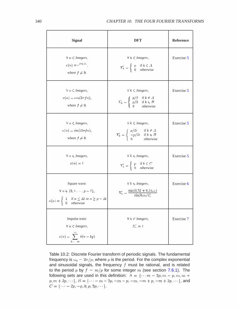
340 CHAPTER 10. THE FOUR FOURIER TRANSFORMS
Signal DFT Reference
� � � Integers�
���� � ���� ��
where � �� �.
� � � Integers�
� �� �
�� if � � �� otherwise
Exercise 5
� � � Integers�
���� � ���������
where � �� �.
� � � Integers�
� �� �
���� if � � ���� if � � � otherwise
Exercise 5
� � � Integers�
���� � ����������
where � �� �.
� � � Integers�
� �� �
����� if � � ������ if � � � otherwise
Exercise 5
� � � Integers�
���� � �
� � � Integers�
� �� �
�� if � � �� otherwise
Exercise 5
Square wave:
� � � �� �� � � � � �� ���
���� �
�� if � � or � � ���� otherwise
� � � Integers�
� �� �
������ � � �����
���������
Exercise 6
Impulse train:
� � � Integers�
���� �
���
��� ���
� � � Integers�
� �� � �
Exercise 7
Table 10.2: Discrete Fourier transform of periodic signals. The fundamentalfrequency is �� � ���(, where ( is the period. For the complex exponentialand sinusoidal signals, the frequency � must be rational, and is relatedto the period ( by � � '�( for some integer ' (see section 7.6.1). Thefollowing sets are used in this definition: � � � ' � �(�' � (�'�' �(�'� �(� , � � � �'� �(��'� (��'��'� (��'� �(� , and� � � � �(��(� � (� �(� .
10.4. THE DISCRETE-TIME FOURIER TRANSFORM (DTFT) 341
Other examples of discrete Fourier transform coefficients for various signals are given in table10.2.
10.4 The discrete-Time Fourier transform (DTFT)
We have shown in section 9.2 that the frequency response ; of an LTI system is related to theimpulse response � by
� � Reals� ;��� ���
����
��'�������
; is called the discrete-time Fourier transform (DTFT) of �. For any � DiscSignals(not justan impulse response), its DTFT is defined to be
� � Reals� ���� ���
������'������� (10.11)
Of course, this definition is only valid for those � and those � where the sum converges (it is nottrivial mathematically to characterize this).
Notice that the function � is periodic with period ��. That is, ���� � �������� for any integer� , because
����� � ��� ���)���
for any integer � . Thus, � ContPeriodic�).
Note that (10.11) looks like a discrete Fourier series expansion of the periodic function � . That is,the periodic function is described as a sum of complex exponentials. The only substantial difference,comparing with (10.1), is the sign of the exponent. This sign difference can be easily removed witha change of variables. By doing so, you can discover that ����� is the �-th Fourier series coefficientfor the function �!
The DTFT (10.11) has similar structure to the DFT (10.9). In fact, the DTFT can be viewed asa generalization of the DFT to signals that are neither periodic nor finite. In other words, as (approaches infinity, �� approaches zero, so instead of a discrete set of frequencies spaced by �� wehave a continuum.
The DTFT is a systemDTFT�DiscSignals� ContPeriodic�)
and its inverse isInverseDTFT�ContPeriodic�) � DiscSignals�
The inverse is given by
� � Integers� ���� � ��)
�)"������������ (10.12)

342 CHAPTER 10. THE FOUR FOURIER TRANSFORMS
x(n)
n1
Figure 10.6: A discrete rectangle signal.
|X(ω)|
ω
4
02πππ/2
Figure 10.7: Magnitude of the DTFT of a discrete rectangle.
Notice that because � is periodic, this can equivalently be written as
� � Integers� ���� �
��
)��)
�����������
We integrate over one cycle of the periodic function, so it does not matter where we start. These aredepicted graphically in figure 10.1(e) and (f).
DTFT and InverseDTFTare inverses of each other. This follows from the fact that FourierSeries#and InverseFourierSeries# are inverses of each other.
Example 10.3: Consider a discrete rectangle � DiscSignals, shown in figure10.6.We can find its DTFT using (10.11) as follows,
���� ���
����
��'������
���
���
������
Notice that when � � , this sum is easy to evaluate because �� � , so
��� � ��
Moreover, when � is any multiple of ��, we get ���� � �, as it should, since theDTFT is periodic with period ��. We can again use the identity (10.10), Letting � � �

10.5. THE CONTINUOUS-TIME FOURIER TRANSFORM 343
x(t)
t1
1
Figure 10.8: A rectangular pulse.
and � � ����, we get
���� �� ����
� �����
The magnitude of this function is plotted in figure10.5.
Other examples of DTFTs for various signals are given in table10.3.
10.5 The continuous-time Fourier transform
The frequency response and impulse response of a continuous-time LTI system are related by thecontinuous-time Fourier transform (CTFT), more commonly called simply the Fourier trans-form (FT),
� � Reals� ���� ��"
������������ (10.13)
The CTFT can be defined for any function � ContSignalswhere the integral exists. It need notbe the impulse response of any system, and it need not be periodic or finite. The inverse relation is
� Reals� ��� � ��)
�"��
����������� (10.14)
It is true but difficult to prove that the CTFT and the inverse CTFT are indeed inverses.
The CTFT can be viewed as a generalization of both the FS and DTFT where neither the frequencydomain nor the time domain signal needs to be periodic. Alternatively, it can be viewed as the lastremaining Fourier transform, where neither time nor frequency is discrete. Graphically, the CTFTis a system as shown in figure 10.1(g) and (h).
Example 10.4: Consider a rectangular pulse � ContSignals, shown in figure10.8.We can find its continuous-time Fourier transform using (10.13) as follows,
���� �
����
���������
�
���
�������
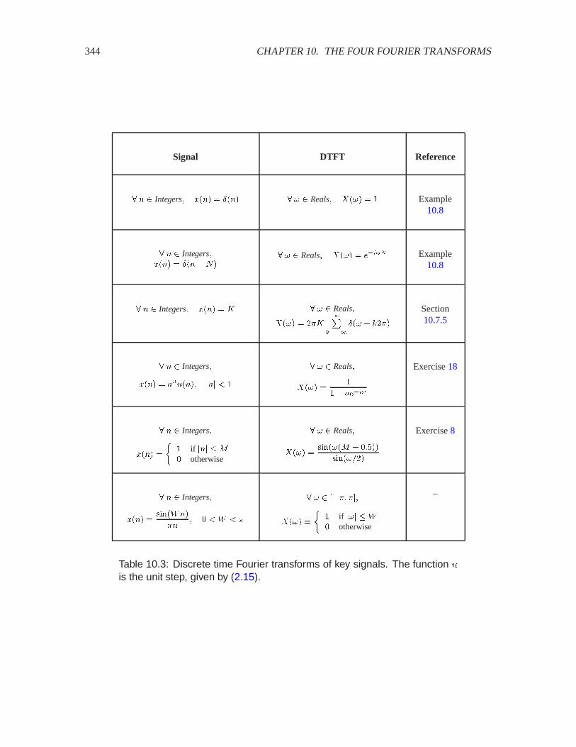
344 CHAPTER 10. THE FOUR FOURIER TRANSFORMS
Signal DTFT Reference
� � � Integers� ���� � ��� � � � Reals� ���� � � Example10.8
� � � Integers����� � �����
� � � Reals� ���� � ���� Example10.8
� � � Integers� ���� � ! � � � Reals�
���� � ��!�
��
�� � ����
Section10.7.5
� � � Integers�
���� � ��"���� � � �
� � � Reals�
���� ��
�� ����
Exercise 18
� � � Integers�
���� �
�� if � �� otherwise
� � � Reals�
���� ������� � � ���
�������
Exercise 8
� � � Integers�
���� ����# ��
��� � � # � �
� � � ���� ���
���� �
�� if � #� otherwise
–
Table 10.3: Discrete time Fourier transforms of key signals. The function 0is the unit step, given by (2.15).
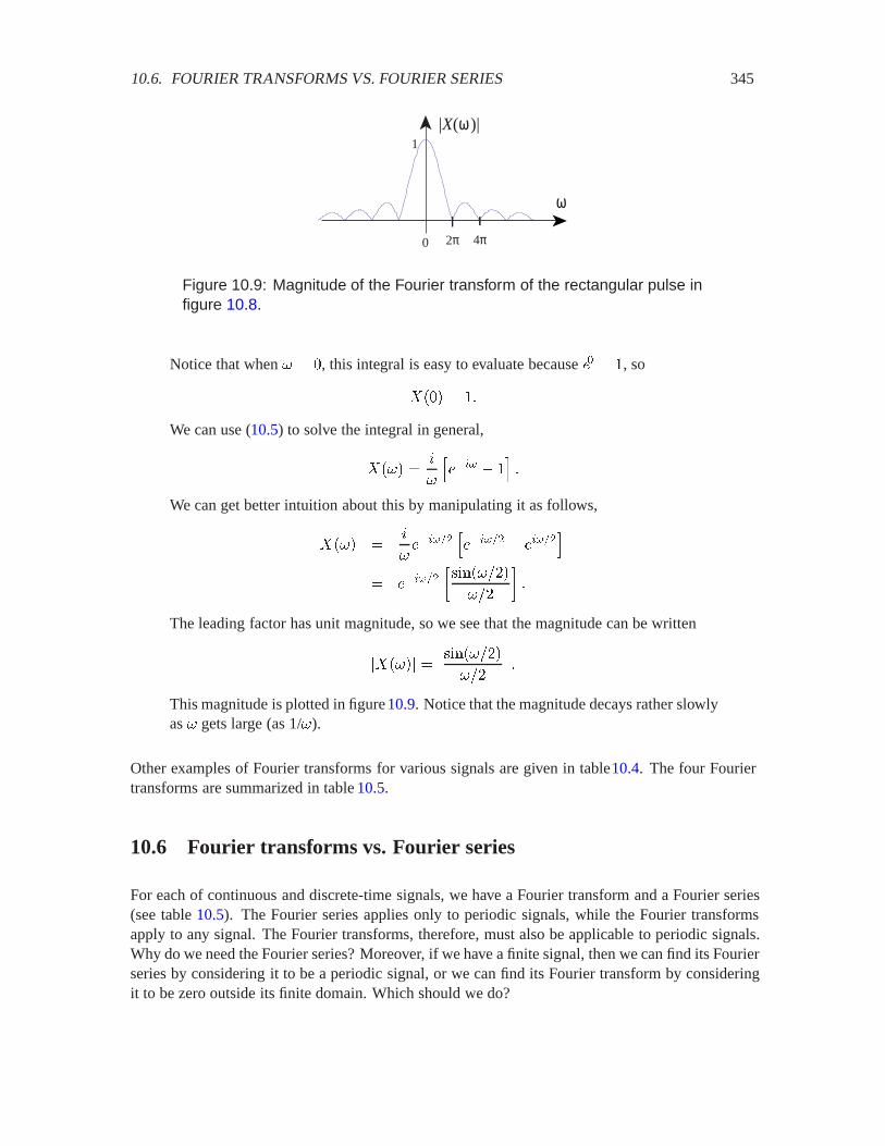
10.6. FOURIER TRANSFORMS VS. FOURIER SERIES 345
|X(ω)|
ω
1
0 2π 4π
Figure 10.9: Magnitude of the Fourier transform of the rectangular pulse infigure 10.8.
Notice that when � � , this integral is easy to evaluate because �� � , so
��� � �
We can use (10.5) to solve the integral in general,
���� �&
�
����� �
��
We can get better intuition about this by manipulating it as follows,
���� �&
�������
������� � �����
�� ������
���������
���
�
The leading factor has unit magnitude, so we see that the magnitude can be written
������ �####�����������
#### �This magnitude is plotted in figure 10.9. Notice that the magnitude decays rather slowlyas � gets large (as 1/�).
Other examples of Fourier transforms for various signals are given in table10.4. The four Fouriertransforms are summarized in table 10.5.
10.6 Fourier transforms vs. Fourier series
For each of continuous and discrete-time signals, we have a Fourier transform and a Fourier series(see table 10.5). The Fourier series applies only to periodic signals, while the Fourier transformsapply to any signal. The Fourier transforms, therefore, must also be applicable to periodic signals.Why do we need the Fourier series? Moreover, if we have a finite signal, then we can find its Fourierseries by considering it to be a periodic signal, or we can find its Fourier transform by consideringit to be zero outside its finite domain. Which should we do?

346 CHAPTER 10. THE FOUR FOURIER TRANSFORMS
Signal CTFT Reference
� � � Reals� ���� � ��� � � � Reals� ���� � � Example10.7
� � � Reals� ���� � ��� ��� � �Reals
� � � Reals� ���� � ���� Example10.7
� � � Reals� ���� � ! � � � Reals� ���� � ��!��� Section10.7.5
� � � Reals�
���� � �"���� � � � � �
� � � Reals�
���� ��
$� � ����
–
� � � Reals�
���� �
���� if � �� otherwise
� � � Reals�
���� ��� ������
��
Exercise 23
� � � Reals�
���� �������� �
�����
� � � Reals�
���� �
�� if � ���� otherwise
Exercise 21
Table 10.4: Continuous time Fourier transforms of key signals. The function0 is the unit step, given by (9.27).
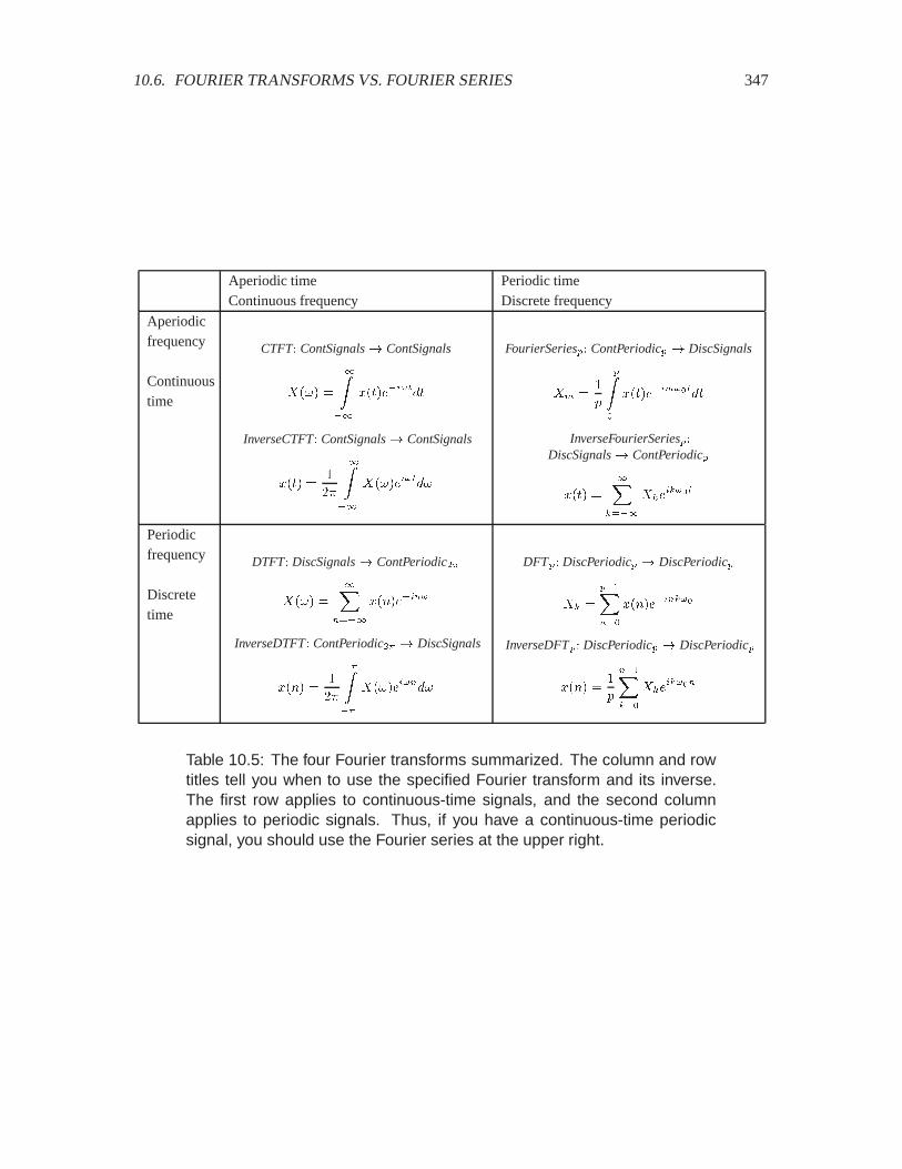
10.6. FOURIER TRANSFORMS VS. FOURIER SERIES 347
Aperiodic timeContinuous frequency
Periodic timeDiscrete frequency
Aperiodicfrequency
Continuoustime
CTFT� ContSignals� ContSignals
���� �
�
�������%�
InverseCTFT� ContSignals� ContSignals
���� ��
��
�
�������%�
FourierSeries� ContPeriodic � DiscSignals
�� ��
�
��
���������%�
InverseFourierSeries�DiscSignals� ContPeriodic
���� �
���
�������
Periodicfrequency
Discretetime
DTFT� DiscSignals� ContPeriodic��
���� �
���
��������
InverseDTFT� ContPeriodic�� � DiscSignals
���� ��
��
���
��������%�
DFT� DiscPeriodic � DiscPeriodic
�� �
�����
����������
InverseDFT� DiscPeriodic � DiscPeriodic
���� ��
�
�����
��������
Table 10.5: The four Fourier transforms summarized. The column and rowtitles tell you when to use the specified Fourier transform and its inverse.The first row applies to continuous-time signals, and the second columnapplies to periodic signals. Thus, if you have a continuous-time periodicsignal, you should use the Fourier series at the upper right.
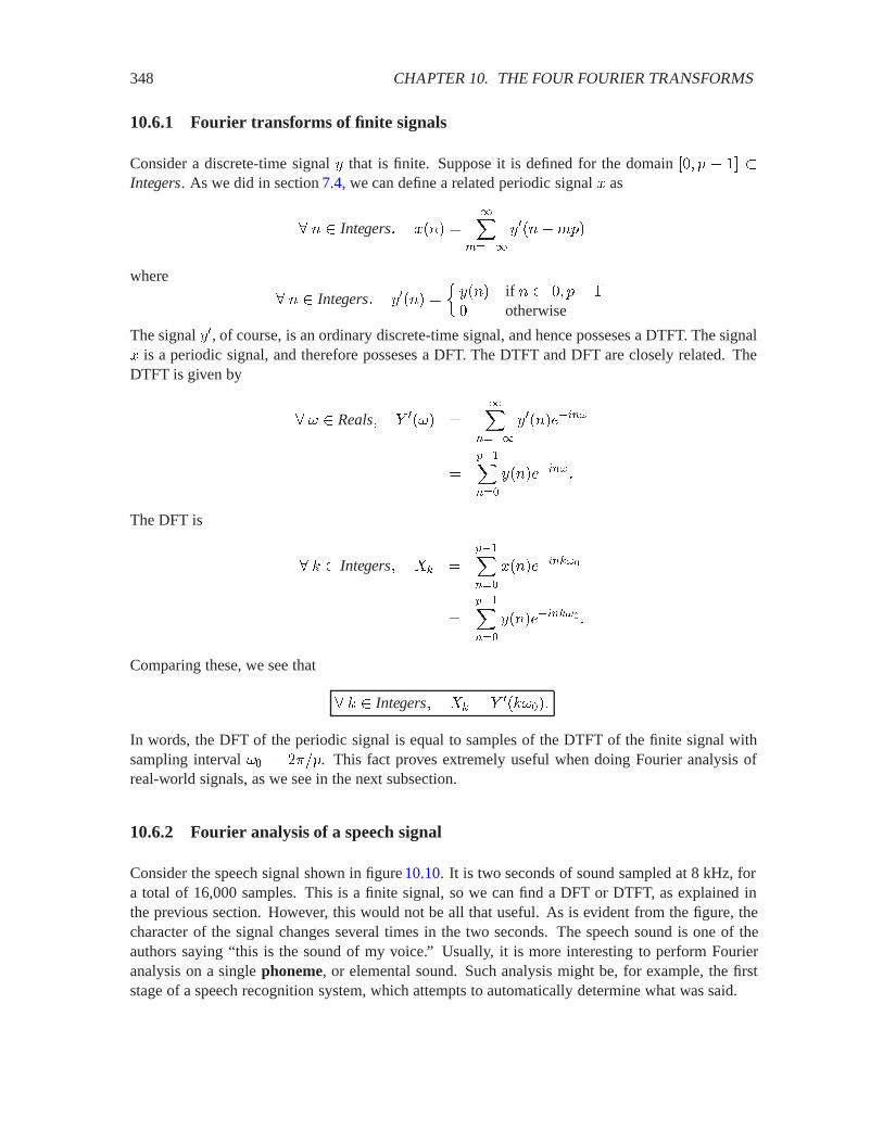
348 CHAPTER 10. THE FOUR FOURIER TRANSFORMS
10.6.1 Fourier transforms of finite signals
Consider a discrete-time signal � that is finite. Suppose it is defined for the domain �� ( � � �Integers. As we did in section 7.4, we can define a related periodic signal � as
� � Integers� ���� ���
����
�����'(�
where
� � Integers� ����� �
����� if � �� (� � otherwise
The signal ��, of course, is an ordinary discrete-time signal, and hence posseses a DTFT. The signal� is a periodic signal, and therefore posseses a DFT. The DTFT and DFT are closely related. TheDTFT is given by
� � Reals� $ ���� ���
����
����������
�#������
����������
The DFT is
� 6 Integers� �� �#������
�����������
�#������
����������� �
Comparing these, we see that
� 6 Integers� �� � $ ��6����
In words, the DFT of the periodic signal is equal to samples of the DTFT of the finite signal withsampling interval �� � ���(. This fact proves extremely useful when doing Fourier analysis ofreal-world signals, as we see in the next subsection.
10.6.2 Fourier analysis of a speech signal
Consider the speech signal shown in figure 10.10. It is two seconds of sound sampled at 8 kHz, fora total of 16,000 samples. This is a finite signal, so we can find a DFT or DTFT, as explained inthe previous section. However, this would not be all that useful. As is evident from the figure, thecharacter of the signal changes several times in the two seconds. The speech sound is one of theauthors saying “this is the sound of my voice.” Usually, it is more interesting to perform Fourieranalysis on a single phoneme, or elemental sound. Such analysis might be, for example, the firststage of a speech recognition system, which attempts to automatically determine what was said.
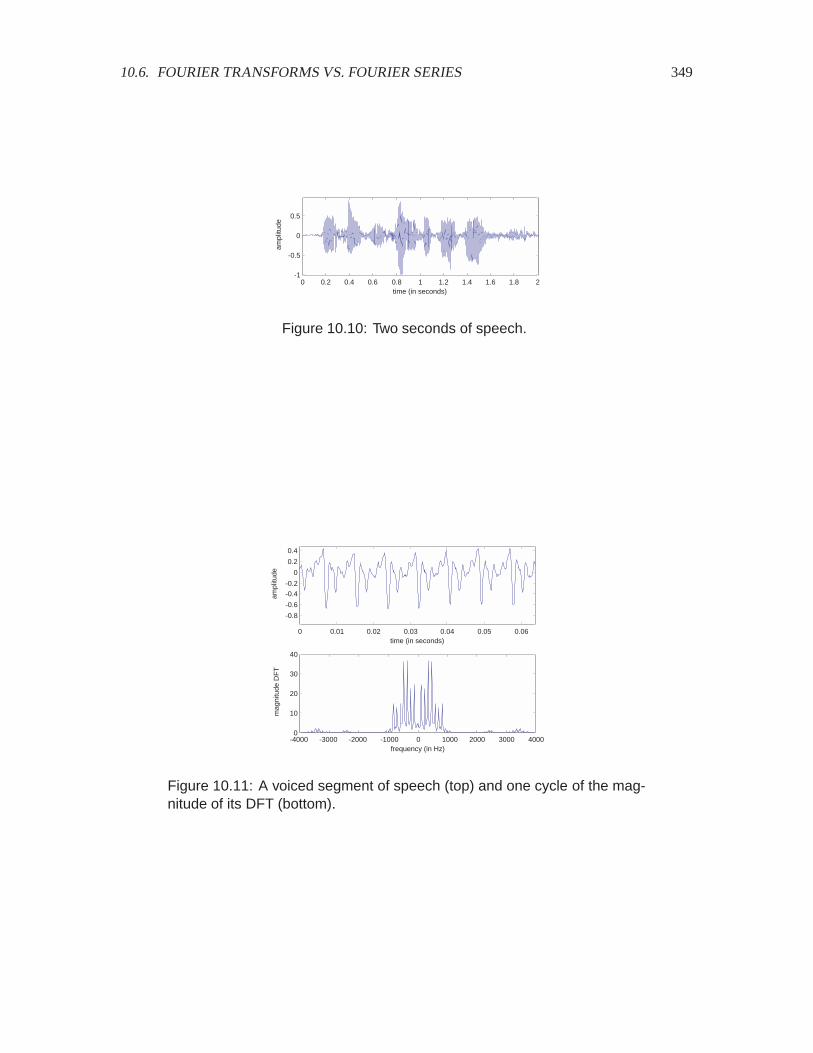
10.6. FOURIER TRANSFORMS VS. FOURIER SERIES 349
0 0.2 0.4 0.6 0.8 1 1.2 1.4 1.6 1.8 2-1
-0.5
0
0.5
time (in seconds)
ampl
itude
Figure 10.10: Two seconds of speech.
0 0.01 0.02 0.03 0.04 0.05 0.06
-0.8
-0.6
-0.4
-0.2
0
0.2
0.4
time (in seconds)
ampl
itude
-4000 -3000 -2000 -1000 0 1000 2000 3000 40000
10
20
30
40
frequency (in Hz)
mag
nitu
de D
FT
Figure 10.11: A voiced segment of speech (top) and one cycle of the mag-nitude of its DFT (bottom).

350 CHAPTER 10. THE FOUR FOURIER TRANSFORMS
-1000 -800 -600 -400 -200 0 200 400 600 800 10000
10
20
30
frequency (in Hz)
mag
nitu
de D
FT
Figure 10.12: DFT of the voiced segment of speech, shown over a narrowerfrequency range.
Consider a much smaller segment of speech shown at the top in figure10.11. This is approximately64 msec of speech, or 512 samples at rate 8,000 samples/second. This particular segment is thevowel sound in the word “sound.” Notice that the signal has quite a bit of structure. Fourier analysiscan reveal a great deal about that structure.
The first issue is to decide which of the four Fourier transforms to apply. This is easy, since thereis only one of the four that is computable, the DFT. Since we do not have an analytic expressionfor the speech signal, we cannot algebraically determine the DTFT. However, we know from theprevious section that the DFT yields samples of the DTFT of a finite signal, so calculating the DFTreveals the structure of the DTFT.
The DFT of these 512 samples is shown at the bottom in figure10.11, which shows one cycle of theperiodic DFT. The horizontal axis is labeled with the frequecies in Hz rather than the index 6 of theDFT coefficient. Recall that the 6-th coefficient of the DFT represents a complex exponential withfrequency 6�� � 6���( radians/sample. To convert this to Hertz, we watch the units,
�6���(��radians/sample���� ��samples/second��������cycles/radian� � 6��( ��cycles/second��
where � �� is the sampling interval.
Although this plot shows the DFT, the plot can equally well be interpreted as a plot of the DTFT.It shows 512 values of the DFT (one cycle of the periodic signal), and instead of showing eachindividual value, it runs them together as a continuous curve. In fact, since the DFT is samples ofthe DTFT, that continuous curve is a pretty good estimate of the shape of the DTFT. Of course, thesamples might not be close together enough to accurately represent the DTFT, but probably theyare. The next chapter will examine this issue in considerable detail.
Notice that most of the signal is concentrated below 1 kHz. In figure10.12, we have zoomed in tothis region of the spectrum. Notice that the DFT is strongly peaked, with the lowest frequency peakoccurring at about 120 Hz. Indeed, this is not surprising, because the time-domain signal at the topof figure 10.11 looks somewhat periodic, with a period of about 80 msec, roughly the inverse of120 Hz. That is, it looks like a periodic signal with fundamental frequency 120 Hz, and variousharmonics. The weights of the harmonics are proportional to the heights of the peaks in figure10.12.
The vowel in the word “sound” is created by vibrating the human vocal chords, and then shaping themouth into an acoustic cavity that alters the sound produced by the vocal chords. A sound that uses

10.6. FOURIER TRANSFORMS VS. FOURIER SERIES 351
0.01 0.02 0.03 0.04 0.05 0.06-0.2
-0.1
0
0.1
time (in seconds)
ampl
itude
-4000 -3000 -2000 -1000 0 1000 2000 3000 40000
2
4
6
8
10
frequency (in Hz)
mag
nitu
de D
FT
Figure 10.13: An unvoiced segment of speech (top) and one cycle of themagnitude of its DFT (bottom).
the vocal chords is called by linguists a voiced sound. By contrast, the “s” in “this” is an unvoicedsound. It is created without the help of the vocal chords by forcing air through a narrow passage inthe mouth to create turbulence.
The “s” in “this” is shown in figure 10.13. It is very different from the vowel sound in 10.11. Inparticular, it looks much less regular. There is no evident periodicity in the signal, so the DFT doesnot reveal a fundamental frequency and harmonics. It is a noise-like signal, where the DFT revealsthat much of the noise is at low frequencies, below 500 Hz, but there are also significant componentsall the way out to 4 kHz.
The analysis we have done on the segments of speech is a typical use of Fourier analysis. A long(even infinite) signal is divided into short segments, such as the two 512-sample segments that weexamined above. These segments are studied by calculating their DFT. Since the DFT is a finitesummation, it is easy to realize on a computer. Also, as mentioned before, there is a highly efficientalgorithm called the fast Fourier transform or FFT to calculate the DFT. The fft function inMatlab was used to calculate the DFTs in figures 10.11 and 10.13. The DFT yields samples ofthe DTFT of the finite segment of signal. This idea is explored in much more detail in lab C.7,where it is shown how to repeatedly calculate DFTs of short segments to create a spectrogram.The spectrogram for the signal in figure 10.10 is shown in figure C.8.
10.6.3 Fourier transforms of periodic signals
In the previous two sections, we have seen the relationship between the DTFT of a finite signal andthe DFT of the periodic signal that is constructed by repeating the finite signal. The periodic signal,however, also has a DTFT itself. In the interest of variety, we will explore this concept in continuoustime.
A periodic continuous-time signal has a Fourier transform. But, as we will see, that Fourier trans-form has Dirac delta functions in it, which are mathematically tricky. Recall that a Dirac delta
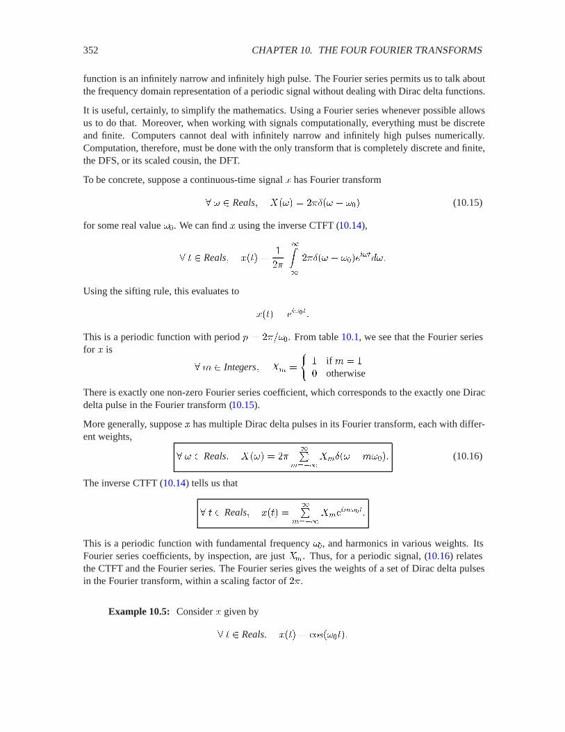
352 CHAPTER 10. THE FOUR FOURIER TRANSFORMS
function is an infinitely narrow and infinitely high pulse. The Fourier series permits us to talk aboutthe frequency domain representation of a periodic signal without dealing with Dirac delta functions.
It is useful, certainly, to simplify the mathematics. Using a Fourier series whenever possible allowsus to do that. Moreover, when working with signals computationally, everything must be discreteand finite. Computers cannot deal with infinitely narrow and infinitely high pulses numerically.Computation, therefore, must be done with the only transform that is completely discrete and finite,the DFS, or its scaled cousin, the DFT.
To be concrete, suppose a continuous-time signal � has Fourier transform
� � Reals� ���� � ���� � ��� (10.15)
for some real value ��. We can find � using the inverse CTFT (10.14),
� Reals� ��� �
��
����
���� � ����������
Using the sifting rule, this evaluates to
��� � ������
This is a periodic function with period ( � �����. From table 10.1, we see that the Fourier seriesfor � is
�' Integers� �� �
� if ' � otherwise
There is exactly one non-zero Fourier series coefficient, which corresponds to the exactly one Diracdelta pulse in the Fourier transform (10.15).
More generally, suppose � has multiple Dirac delta pulses in its Fourier transform, each with differ-ent weights,
� � Reals� ���� � ����
�������� �'���� (10.16)
The inverse CTFT (10.14) tells us that
� Reals� ��� ���
�������
������
This is a periodic function with fundamental frequency ��, and harmonics in various weights. ItsFourier series coefficients, by inspection, are just ��. Thus, for a periodic signal, (10.16) relatesthe CTFT and the Fourier series. The Fourier series gives the weights of a set of Dirac delta pulsesin the Fourier transform, within a scaling factor of ��.
Example 10.5: Consider � given by
� Reals� ��� � ��������
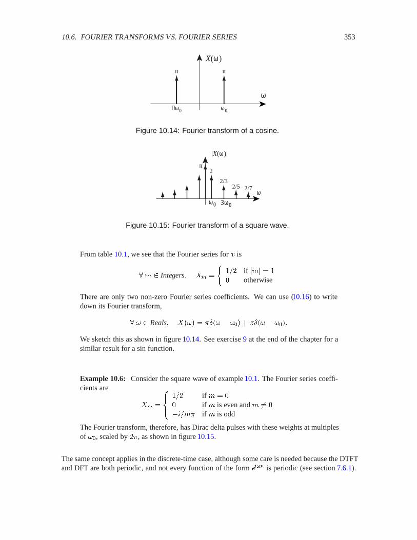
10.6. FOURIER TRANSFORMS VS. FOURIER SERIES 353
X(ω)
ω
π
ω0
π
−ω0
Figure 10.14: Fourier transform of a cosine.
|X(ω)|
ω
π2
2/32/5 2/7
ω0 3ω0
Figure 10.15: Fourier transform of a square wave.
From table 10.1, we see that the Fourier series for � is
�' Integers� �� �
��� if �'� � otherwise
There are only two non-zero Fourier series coefficients. We can use (10.16) to writedown its Fourier transform,
� � Reals� ���� � ��� � ��� � ��� � ����
We sketch this as shown in figure 10.14. See exercise 9 at the end of the chapter for asimilar result for a sin function.
Example 10.6: Consider the square wave of example 10.1. The Fourier series coeffi-cients are
�� �
����
�� if ' � if ' is even and ' �� �&�'� if ' is odd
The Fourier transform, therefore, has Dirac delta pulses with these weights at multiplesof ��, scaled by ��, as shown in figure 10.15.
The same concept applies in the discrete-time case, although some care is needed because the DTFTand DFT are both periodic, and not every function of the form ���� is periodic (see section 7.6.1).
354 CHAPTER 10. THE FOUR FOURIER TRANSFORMS
In fact, in figure 10.11, the peaks in the spectrum hint at the Dirac delta functions in the DTFT.The signal appears to be roughly periodic with period 120 Hz, so the DFT shows strong peaks atmultiples of 120 Hz. If the signal were perfectly periodic, and if we were plotting the DTFT insteadof the DFT, then these peaks would become infinitely narrow and infinitely high.
10.7 Properties of Fourier transforms
In this section, we give a number of useful properties of the various Fourier transforms, togetherwith a number of illustrative examples. These properties are summarized in tables 10.6 through10.9. The properties and examples can often be used to avoid solving integrals or summations tofind the Fourier transform of some signal, or to find an inverse Fourier transform.
10.7.1 Convolution
Suppose a discrete-time LTI system has impulse response � and frequency response ; . We haveseen that if the input to this system is a complex exponential, ����, then the output is ;�������.Suppose the input is instead an arbitrary signal � with DTFT � . Using the inverse DTFT relation,we know that
� � Integers� ���� �
��
�)��
�����������
View this as a summation of exponentials, each with weight ����. An integral, after all, is sum-mation over a continuum. Each term in the summation is ��������. If this term were an inputby itself, then the output would be ;�����������. Thus, by linearity, if the input is �, the outputshould be
� � Integers� ���� �
��
�)��
;�������������
Comparing to the inverse DTFT relation for ����, we see that
� � Reals� $ ��� � ;�������� (10.17)
This is the frequency-domain version of convolution
� � Integers� ���� � �� � ������
Thus, the frequency response of an LTI system multiplies the DTFT of the input. This is intuitive,since the frequency response gives the weight imposed by the system on each frequency componentof the input.
Equation (10.17) applies equally well to continuous-time systems, but in that case, ; is the CTFTof the impulse response, and � is the CTFT of the input.
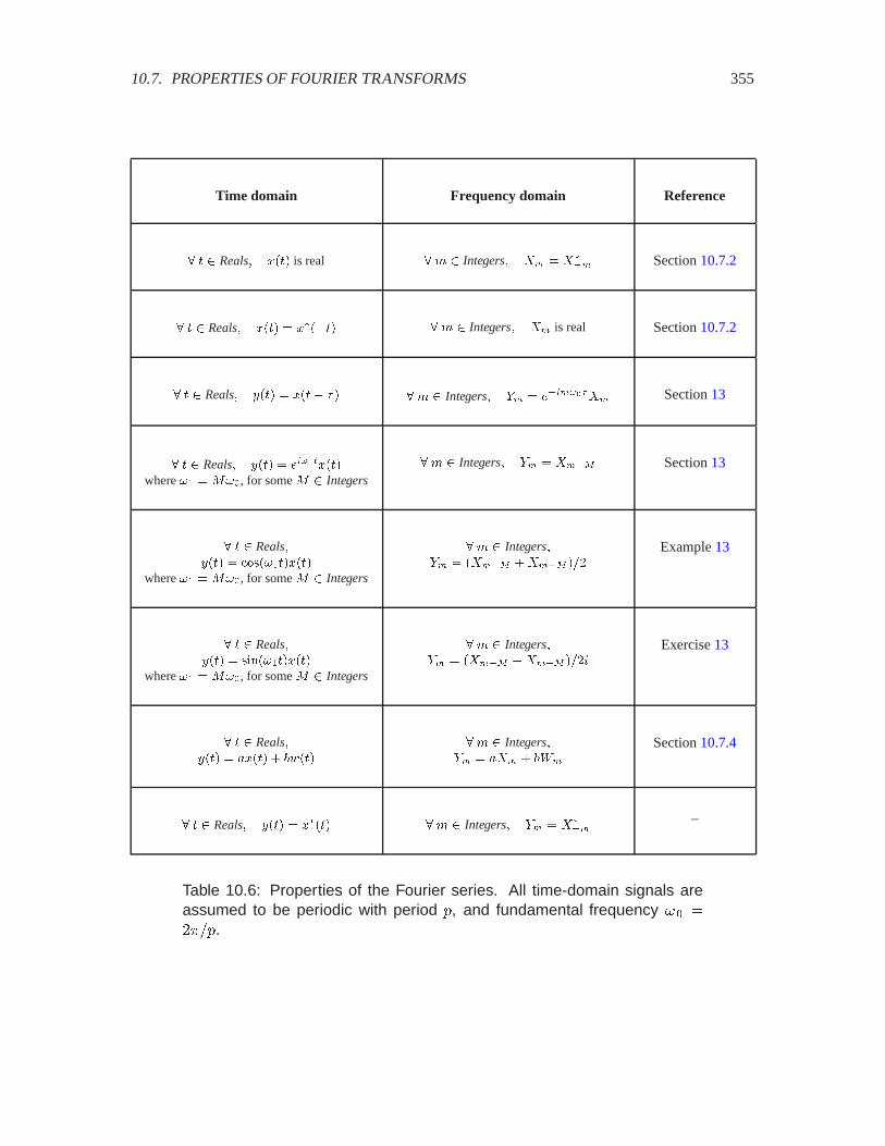
10.7. PROPERTIES OF FOURIER TRANSFORMS 355
Time domain Frequency domain Reference
� � � Reals� ���� is real � � � Integers� �� � ��� Section 10.7.2
� � � Reals� ���� � ������ � � � Integers� �� is real Section 10.7.2
� � � Reals� &��� � ���� � � � � � Integers� '� � �������� Section 13
� � � Reals� &��� � ��������where �� � ���, for some � � Integers
� � � Integers� '� � ��� Section 13
� � � Reals�&��� � �����������
where �� � ���, for some � � Integers
� � � Integers�'� � ���� � ���� ���
Example 13
� � � Reals�&��� � �����������
where �� � ���, for some � � Integers
� � � Integers�'� � ���� ����� ����
Exercise 13
� � � Reals�&��� � ����� � ()���
� � � Integers�'� � ��� � (#�
Section 10.7.4
� � � Reals� &��� � ����� � � � Integers� '� � ���
–
Table 10.6: Properties of the Fourier series. All time-domain signals areassumed to be periodic with period (, and fundamental frequency �� ����(.
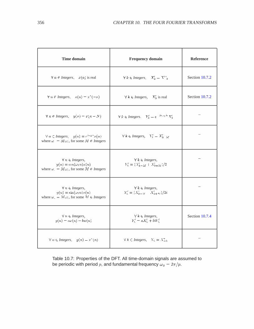
356 CHAPTER 10. THE FOUR FOURIER TRANSFORMS
Time domain Frequency domain Reference
� � � Integers� ���� is real � � � Integers� ��� � � ��
� Section 10.7.2
� � � Integers� ���� � ������ � � � Integers� ��� is real Section 10.7.2
� � � Integers� &��� � ������ � � � Integers� ' �� � ������� �
�
–
� � � Integers� &��� � ���������where �� � ���, for some � � Integers
� � � Integers� ' �� � � �
��–
� � � Integers�&��� � �����������
where �� � ���, for some � � Integers
� � � Integers�' �� � �� �
�� � � ���� ���
–
� � � Integers�&��� � �����������
where �� � ���, for some � � Integers
� � � Integers�' �� � �� �
�� �� ���� ����
–
� � � Integers�&��� � ����� � ()���
� � � Integers�' �� � �� �
� � (# ��
Section 10.7.4
� � � Integers� &��� � ����� � � � Integers� '� � ���
–
Table 10.7: Properties of the DFT. All time-domain signals are assumed tobe periodic with period (, and fundamental frequency �� � ���(.

10.7. PROPERTIES OF FOURIER TRANSFORMS 357
Time domain Frequency domain Reference
� � � Integers� ���� is real � � � Reals� ���� � ������ Section 10.7.2
� � � Integers� ���� � ������ � � � Reals� ���� is real Section 10.7.2
� � � Integers� &��� � ������ � � � Reals� ' ��� � �������� Section 10.7.3
� � � Integers� &��� � ��������� � � � Reals� ' ��� � ��� � ��� Section 10.7.6
� � � Integers�&��� � �����������
� � � Reals�' ��� � ���� � ��� � ��� � ������
Example 10.11
� � � Integers�&��� � �����������
� � � Reals�' ��� � ���� � ������� � �������
Exercise 12
� � � Integers����� � ������ � (�����
� � � Reals����� � ������ � (�����
Section 10.7.4
� � � Integers� &��� � �* � ����� � � � Reals� ' ��� � +������� Section 10.7.1
� � � Integers� &��� � �������� � � � Reals�
' ��� � ���
��"�
����, �� � ��%�
Box on page 359
� � � Integers�
&��� �
������� � is a multiple of �� otherwise
� � � Reals�' ��� � �����
Exercise 14
Table 10.8: Properties of the DTFT.
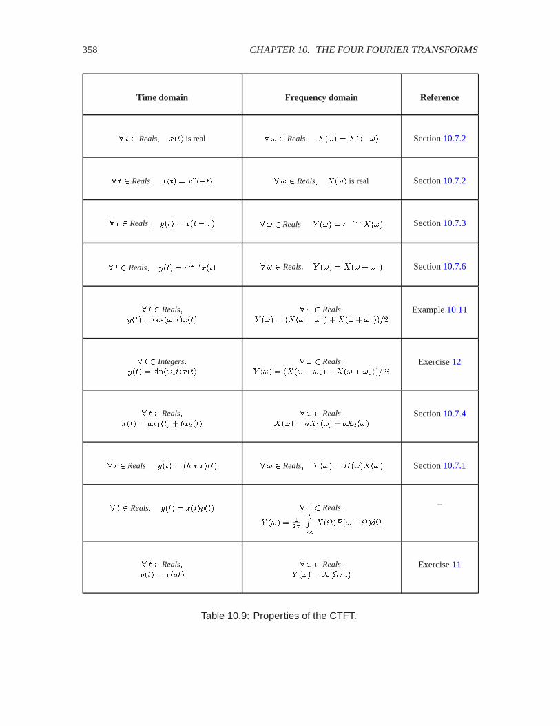
358 CHAPTER 10. THE FOUR FOURIER TRANSFORMS
Time domain Frequency domain Reference
� � � Reals� ���� is real � � � Reals� ���� � ������ Section 10.7.2
� � � Reals� ���� � ������ � � � Reals� ���� is real Section 10.7.2
� � � Reals� &��� � ���� � � � � � Reals� ' ��� � �������� Section 10.7.3
� � � Reals� &��� � �������� � � � Reals� ' ��� � ��� � ��� Section 10.7.6
� � � Reals�&��� � �����������
� � � Reals�' ��� � ���� � ��� � ��� � ������
Example 10.11
� � � Integers�&��� � �����������
� � � Reals�' ��� � ���� � ������� � �������
Exercise 12
� � � Reals����� � ������ � (�����
� � � Reals����� � ������ � (�����
Section 10.7.4
� � � Reals� &��� � �* � ����� � � � Reals� ' ��� � +������� Section 10.7.1
� � � Reals� &��� � �������� � � � Reals�
' ��� � ���
"
����, �� ���%�
–
� � � Reals�&��� � �����
� � � Reals�' ��� � ������
Exercise 11
Table 10.9: Properties of the CTFT.
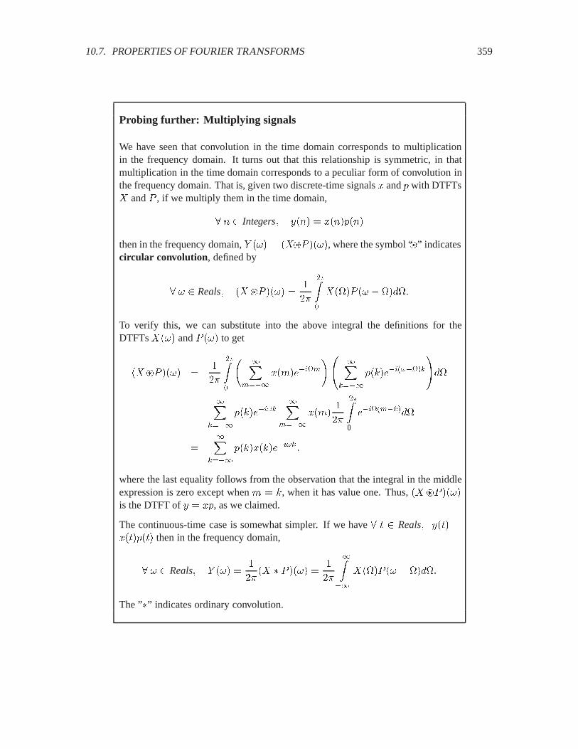
10.7. PROPERTIES OF FOURIER TRANSFORMS 359
Probing further: Multiplying signals
We have seen that convolution in the time domain corresponds to multiplicationin the frequency domain. It turns out that this relationship is symmetric, in thatmultiplication in the time domain corresponds to a peculiar form of convolution inthe frequency domain. That is, given two discrete-time signals � and ( with DTFTs� and � , if we multiply them in the time domain,
� � Integers� ���� � ����(���
then in the frequency domain, $ ��� � �� ��� ����, where the symbol “��” indicatescircular convolution, defined by
� � Reals� �� ��� ���� �
��
�)��
����� �� � �����
To verify this, we can substitute into the above integral the definitions for theDTFTs ���� and � ��� to get
�� ��� ���� �
��
�)��
���
����
��'������
�$% ������
(�6���� �����
&'��
���
����
(�6��������
����
��'�
��
�)��
���� ������
���
����
(�6���6������ �
where the last equality follows from the observation that the integral in the middleexpression is zero except when ' � 6, when it has value one. Thus, �� ��� ����is the DTFT of � � �(, as we claimed.
The continuous-time case is somewhat simpler. If we have � Reals� ��� ����(�� then in the frequency domain,
� � Reals� $ ��� �
���� � � ���� �
��
����
����� �� � �����
The ”�” indicates ordinary convolution.
360 CHAPTER 10. THE FOUR FOURIER TRANSFORMS
10.7.2 Conjugate symmetry
We have already shown (see (8.29)) that for real-valued signals, the Fourier series coefficients areconjugate symmetric,
�� � �����
In fact, all the Fourier transforms are conjugate symmetric if the time-domain function is real.We illustrate this with the CTFT. Suppose ��Reals� Realsis a real-valued signal, and let � �CTFT���. In general, ���� will be complex-valued. However, from (10.13), we have
�������� �
� �
�������������
�
� �
�����������
� �����
Thus,���� � �������
i.e. for real-valued signals, ���� and ����� are complex conjugates of one another.
We can show that, conversely, if the Fourier transform is conjugate symmetric, then the time-domainfunction is real. To do this, write the inverse CTFT
��� �
��
����
����������
and then conjugate both sides,
���� �
��
����
�������������
By changing variables (replacing � with��) and using the conjugate symmetry of � , we can showthat
���� � ����
which implies that ��� is real for all .
The inverse Fourier transforms can be used to show that if a time-domain function is conjugatesymmetric,
��� � ������then its Fourier transform is real. The same property applies to all four Fourier transforms.
In summary, if a function in one domain (time or frequency) is conjugate symmet-ric, then the function in the other domain (frequency or time) is real.
10.7. PROPERTIES OF FOURIER TRANSFORMS 361
10.7.3 Time shifting
Given a continuous-time function � and its Fourier transform � � CTFT���, let � be defined by
� Reals� ��� � ��� ��
for some real constant � . This is called time shifting or delay. We can find $ � CTFT��� in termsof � as follows,
$ ��� �
����
���������
�
����
��� ��������
�
����
������� ��(��
� ����(
����
���������
� ����(�����
Thus, in summary,
��� � ��� �� � $ ��� � ����(����� (10.18)
The bidirectional arrow indicates that this relationship works both ways. If you know that $ ��� �����(����, then you can conclude that ��� � ��� ��.
Example 10.7: One of the simplest Fourier transforms to compute is that of � when
��� � ���
where Æ is the Dirac delta function. Plugging into the formula,
���� �
����
���������
�
����
��������
� �����
� �
362 CHAPTER 10. THE FOUR FOURIER TRANSFORMS
where we have used the sifting property of the delta function. The Fourier transformis a constant, 1.1 This indicates that the Dirac delta function, interestingly, contains allfrequencies in equal amounts.
Moreover, this result is intuitive if one considers an LTI system with impulse response��� � ��. Such a system responds to an impulse by producing an impulse, whichsuggests that any input will be simply passed through unchanged. Indeed, its frequencyresponse is ;��� � for all � Reals, so given an input � with Fourier transform � ,the output � has Fourier transform
$ ��� � ;������� � �����
Since the output has the same Fourier transform as the input, the output is the same asthe input.
Using (10.18), we can now find the Fourier transform of another signal
��� � � � ���
for some constant � Reals. It is
���� � ����( �
Note that, as required, this is conjugate symmetric. Moreover, it has magnitude 1. Itsphase is ��� , a linear function of �.
Again, we can gain some intuition by considering an LTI system with impulse response
��� � �� ��� (10.19)
Such a system introduces a fixed time delay of � . Its frequency response is
;��� � ����( � (10.20)
Since this has magnitude 1 for all �, it tells us that all frequencies get through the delaysystem unattenuated, as expected. However, each frequency � will experience a phaseshift of ��� , corresponding to a time delay of � .
Discrete-time signals are similar. Consider a discrete-time signal � with � � DTFT���, and let �be defined by
� Reals� ���� � ������
for some integer constant � . By similar methods, we can find that
���� � ������ � $ ��� � ���������� (10.21)
1To see how the sifting property works, note that the integrand is zero everywhere except where � � �, at which pointthe complex exponential evaluates to 1. Then the integral of the delta function itself has value one.

10.7. PROPERTIES OF FOURIER TRANSFORMS 363
Example 10.8: Suppose we have a discrete-time signal � given by
���� � ����
where Æ is the Kronecker delta function. It is easy to show from the DTFT definitionthat
���� � �
Using (10.21), we can now find the Fourier transform of another signal
���� � ������
for some constant � Integers. It is
���� � ����� �
Notice that if � � , this reduces to ���� � , as expected.
10.7.4 Linearity
Consider three discrete-time signals �, ��, ��, related by
� � Integers� ���� � ������ � �������
Then it is easy to see from the definition of the DTFT that
� � Reals� ���� � ������ � ������
where � � DTFT���, �� � DTFT����, and �� � DTFT����.
The same linearity property applies to the CTFT,
��� � ����� � ����� � ���� � ������ � ������
Linearity of the Fourier transform is one of the most useful properties for avoiding evaluation ofintegrals and summations.
Example 10.9: Consider for example the discrete-time signal � given by
���� � ��� � � ��� ��
where Æ is the Kronecker delta function. Using linearity, we know that the DTFT of� is the sum of the DTFT of Æ�� � � and the DTFT of Æ�� � �. From the previousexample, we know those two DTFTs, so
���� � ��� � ����
because � is � and 1, respectively. Using Euler’s relation, we can simplify this to get
���� � � �������
Interestingly, the DTFT of this example turns out to be real. This is because the time-domain function is conjugate symmetric (the conjugate of something real is itself).Moreover, since it is real in the time domain, the DTFT turns out to be conjugatesymmetric.
364 CHAPTER 10. THE FOUR FOURIER TRANSFORMS
Linearity can also be used to find inverse Fourier transforms.
Example 10.10: Suppose you are told that a continuous-time signal has Fourier trans-form
���� � �������
How would you find the time-domain function? You could evaluate the inverse CTFT,but the integration that you would have to perform is quite difficult. Instead, use Euler’srelation to write
���� � ���� � ��������
Then use linearity. The inverse Fourier transform of this sum will be the sum of theinverse Fourier transforms of the terms. These we can recognize from (10.19) and(10.20), so
��� � �� � � � �� �����
where Æ is the Dirac delta function.
10.7.5 Constant signals
We have seen that the Fourier transform of a delta function is a constant. With the symmetriesthat we have observed between time and frequency, it should come as no surprise that the Fouriertransform of a constant is a delta function.
Consider first a continuous-time signal � given by
� Reals� ��� � >
for some real constant > . Its CTFT is
���� � >
����
�������
which is not easy to evaluate. This integral is mathematically subtle. The answer is
� � Reals� ���� � ��>����
where Æ is the Dirac delta function. What this says is that a constant in the time domain is concen-trated at zero frequency in the frequency domain (which should not be surprising). Except for themultiplying constant of ��, we probably could have guessed this answer. We can verify this answerby evaluating the inverse CTFT,
��� �
��
����
����������
� >
����
���������
� >�
10.7. PROPERTIES OF FOURIER TRANSFORMS 365
where the final step follows from the sifting property of the Dirac delta function. Thus, in summary,
��� � > � ���� � ��>��� (10.22)
The discrete-time case is similar, but there is one subtlety because the DTFT is periodic. Let � be adiscrete time signal where
� � Integers� ���� � >
for some real constant > . Its DTFT is
� � ���� ��� ���� � ��>����
where Æ is the Dirac delta function. This is easy to verify using the inverse DTFT. Again, what thissays is that a constant in the time domain is concentrated at zero frequency in the frequency domain(which should not be surprising). However, recall that a DTFT is periodic with period ��, meaningthat for all integers � ,
���� � ��� ������
Thus, in addition to a delta function at � � , there must be one at � � ��, � � ���, � � ��, etc.This can be written using a shift-and-add summation,
� � Reals� ���� � ��>��
����
�� � 6����
Thus, in summary,
���� � > � ���� � ��>��
������ � 6���� (10.23)
10.7.6 Frequency shifting and modulation
Suppose that � is a continuous-time signal with CTFT � . Let � be another continuous-time signaldefined by
��� � ��������
for some real constant ��. The CTFT of � is easy to compute,
$ ��� �
����
���������
�
����
��������������
�
����
������ �������
� ��� � ����
366 CHAPTER 10. THE FOUR FOURIER TRANSFORMS
Thus, the Fourier transform of � is the same as that of �, but shifted to the right by ��. In summary,
��� � �������� � $ ��� � ��� � ���� (10.24)
This result can be used to determine the effect of multiplying a signal by a sinusoid, a process calledmodulation (see exercise 16 and lab C.10).
Example 10.11: Suppose
��� � ��� ��������
Use Euler’s relation to rewrite this
��� � ��������� � ����������
Then use (10.24) to get the CTFT,
$ ��� � ���� � ��� ���� � �������
We can combine (10.24) with (10.22) to get the following facts:
��� � ����� � ���� � ���� � ���� (10.25)
This says that a complex exponential signal with frequency �� is concentrated in the frequencydomain at frequency ��, which should not be surprising. Similarly,
��� � ������� � ���� � ���� � ��� � �� � ����� (10.26)
We can get a similar set of results for discrete-time signals. We summarize the results here, andleave their verification to the reader (see exercise14):
���� � ��������� � $ ��� � ��� � ���� (10.27)
���� � ���� �������� � $ ��� � ���� � ��� ���� � ������� (10.28)
���� � ����� � ���� � ����
������ � �� � 6���� (10.29)
���� � �������� � ���� � ���
������� � �� � 6��� � �� � �� � 6����� (10.30)
Additional properties of Fourier transforms are explored in the exercises.
10.8. SUMMARY 367
10.8 Summary
In previous chapters, we developed the result that signals can be represented as sums of sinusoids.We used this representation to analyze the effect that a linear time invariant system has on signals.We variously considered periodic and non-periodic signals and impulse and frequency responses ofLTI systems.
In this chapter, we unified all frequency domain discussion by showing that there are four closelyinterrelated Fourier transforms. Two of these apply to discrete-time signals, and two apply tocontinuous-time signals. Two of them apply to periodic signals, and two of them apply to non-periodic signals.
The four Fourier transforms can be viewed as generalizations of the Fourier series. Consequently,they share many properties that are rooted in the Fourier series. These properties can be leveragedto analyze more complicated signals by using an analysis of simpler signals.
Exercises
Each problem is annotated with the letter E, T, C which stands for exercise, requires some thought,requires some conceptualization. Problems labeled E are usually mechanical, those labeled T re-quire a plan of attack, those labeled C usually have more than one defensible answer.
1. E Show that if two discrete-time systems with frequency responses ;���� and ;���� areconnected in cascade, that the DTFT of the output is given by $ ��� � ;����;��������,where ���� is the DTFT of the input.
2. E This exercise verifies some of the relations in table10.1.
(a) Let � be given by
� Reals� ��� � ������
where �� �� . Use (10.2) to verify that its Fourier series coefficients are
�' Integers� �� �
� if ' � otherwise
(b) Let � be given by
� Reals� ��� � ��������
where �� �� . Use part (a) and properties of the Fourier series to verify that its Fourierseries coefficients are
�' Integers� �� �
��� if �'� � otherwise
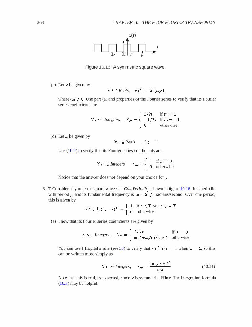
368 CHAPTER 10. THE FOUR FOURIER TRANSFORMS
x(t)
t1
T p−p −T
Figure 10.16: A symmetric square wave.
(c) Let � be given by� Reals� ��� � ��������
where �� �� . Use part (a) and properties of the Fourier series to verify that its Fourierseries coefficients are
�' Integers� �� �
����
��& if ' � ���& if ' � � otherwise
(d) Let � be given by� Reals� ��� � �
Use (10.2) to verify that its Fourier series coefficients are
�' Integers� �� �
� if ' � otherwise
Notice that the answer does not depend on your choice for (.
3. T Consider a symmetric square wave � ContPeriodic#, shown in figure 10.16. It is periodicwith period (, and its fundamental frequency is �� � ���( radians/second. Over one period,this is given by
� �� (�� ��� �
� if ) or 2 (� otherwise
(a) Show that its Fourier series coefficients are given by
�' Integers� �� �
���( if ' � ����'�� ���'�� otherwise
You can use l’Hopital’s rule (see 53) to verify that �������� � when � � , so thiscan be written more simply as
�' Integers� �� �����'�� �
'�(10.31)
Note that this is real, as expected, since � is symmetric. Hint: The integration formula(10.5) may be helpful.
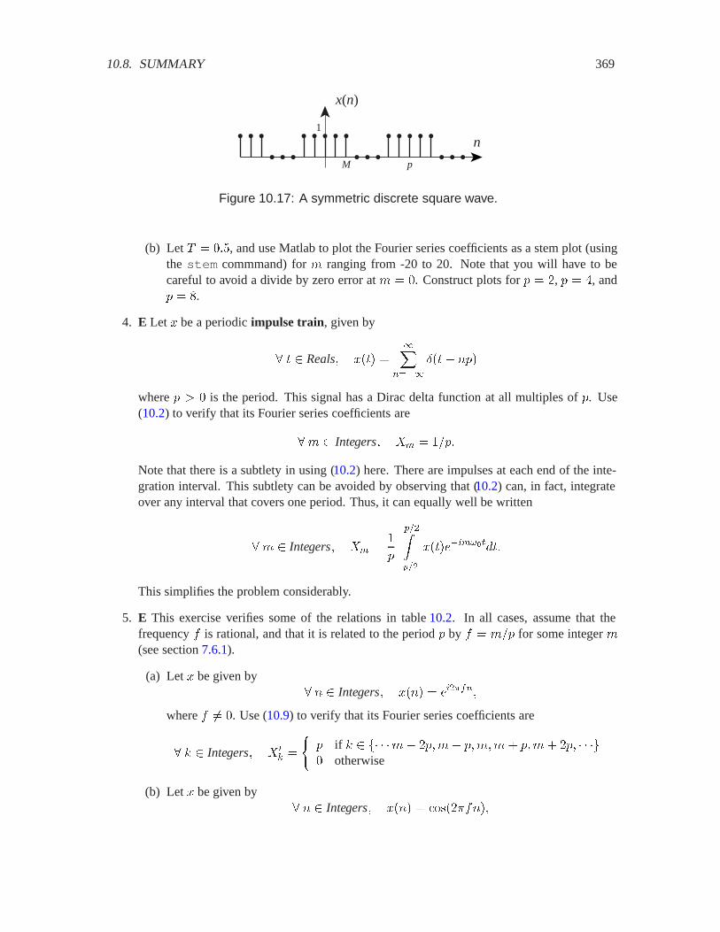
10.8. SUMMARY 369
x(n)
n1
pM
Figure 10.17: A symmetric discrete square wave.
(b) Let � ��, and use Matlab to plot the Fourier series coefficients as a stem plot (usingthe stem commmand) for ' ranging from -20 to 20. Note that you will have to becareful to avoid a divide by zero error at ' � . Construct plots for ( � �, ( � �, and( � �.
4. E Let � be a periodic impulse train, given by
� Reals� ��� ���
����
�� �(�
where ( 2 is the period. This signal has a Dirac delta function at all multiples of (. Use(10.2) to verify that its Fourier series coefficients are
�' Integers� �� � �(�
Note that there is a subtlety in using (10.2) here. There are impulses at each end of the inte-gration interval. This subtlety can be avoided by observing that (10.2) can, in fact, integrateover any interval that covers one period. Thus, it can equally well be written
�' Integers� �� �
(
#����#��
������������
This simplifies the problem considerably.
5. E This exercise verifies some of the relations in table 10.2. In all cases, assume that thefrequency � is rational, and that it is related to the period ( by � � '�( for some integer '(see section 7.6.1).
(a) Let � be given by� � Integers� ���� � ���)$��
where � �� . Use (10.9) to verify that its Fourier series coefficients are
� 6 Integers� ��� �
�( if 6 � '� �(�'� (�'�'� (�'� �(� otherwise
(b) Let � be given by� � Integers� ���� � ����������

370 CHAPTER 10. THE FOUR FOURIER TRANSFORMS
where � �� . Use part (a) and properties of the DFT to verify that its Fourier seriescoefficients are
� �� �
����
(�� if 6 � '� �(�'� (�'�'� (�'� �(� (�� if 6 � �'� �(��'� (��'��'� (��'� �(� otherwise
(c) Let � be given by� � Integers� ���� � ����&������
where � �� . Use part (a) and properties of the DFT to verify that its Fourier seriescoefficients are
� �� �
����
(��& if 6 � '� �(�'� (�'�'� (�'� �(� �(��& if 6 � �'� �(��'� (��'��'� (��'� �(� otherwise
(d) Let � be given by� � Integers� ��� � �
Use (10.9) to verify that its Fourier series coefficients are
�� �
�( if 6 � � �(��(� � (� �(� otherwise
Notice that this result depends on your choice for (. This is a consequence of the unfor-tunate scaling that is used for the DFT, vs. the discrete Fourier series (DFS).
6. T Consider a symmetric discrete square wave � DiscPeriodic#, shown in figure 10.17. Itis periodic with period (, and its fundamental frequency is �� � ���( radians/sample. Overone period, this is given by
� � �� � � (� � ���� �
� if � �3 or � � (�3 otherwise
where, in the figure, 3 � � and ( � �. For this problem, however, assume that 3 and ( canbe any positive integers where ( 2 �3 .
(a) Show that the DFT is given by
� 6 Integers� ��� �
��3 � if 6 is a multiple of (����6�3 � ������� ����6����� otherwise
You can use l’Hopital’s rule (see 53) to verify that ����>��� ������ � > when � � ,so this can be written more simply as
� 6 Integers� ��� �
����6�3 � ������
����6�����(10.32)
Note that this is real, as expected, since � is symmetric. Hint: The summation identityformula (10.10) may be helpful.

10.8. SUMMARY 371
x(n)
n
1
M−M
Figure 10.18: A symmetric discrete rectangle signal.
(b) Let 3 � � and use Matlab to plot the Fourier series coefficients as a stem plot (usingthe stem commmand) for ' ranging from �(� to (� . Note that you will have tobe careful to avoid a divide by zero error at 6 � . Construct plots for ( � �, ( � ,and ( � ��.
7. E Let � be a discrete periodic impulse train, given by
� � Integers� ���� ���
����
���'(�
where ( 2 is the integer period. This signal has a Kronecker delta function at all multiplesof (. Use (10.9) to verify that its DFT coefficients are
� 6 Integers� ��� � �
8. T Consider a symmetric discrete rectangle � DiscSignals, shown in figure10.18. This isgiven by
� � Integers� ���� �
� if ��� �3 otherwise
(a) Show that its DTFT is given by
� � Reals� ���� �������3 � ����
��������
Hint: The summation identity formula (10.10) may be helpful.
(b) Let 3 � � and use Matlab to plot the DTFT with � ranging from �� to (&.
9. E Consider � given by� Reals� ��� � ��������
Show that the CTFT is given by
� � Reals� ���� � ���&��� � ���� ���&��� � ����
10. C In section 10.6 we explored the relationship between the CTFT of a periodic continuous-time signal and its Fourier series. In this problem we do the same for discrete-time signals.
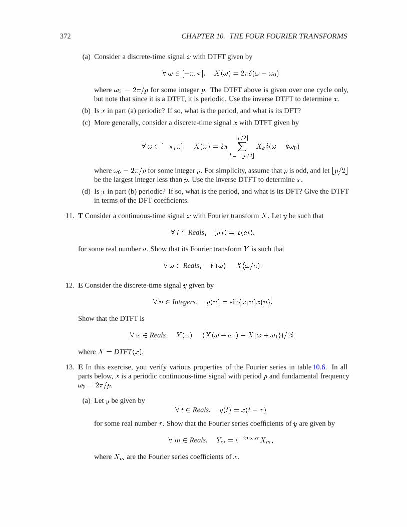
372 CHAPTER 10. THE FOUR FOURIER TRANSFORMS
(a) Consider a discrete-time signal � with DTFT given by
� � ���� ��� ���� � ���� � ���
where �� � ���( for some integer (. The DTFT above is given over one cycle only,but note that since it is a DTFT, it is periodic. Use the inverse DTFT to determine �.
(b) Is � in part (a) periodic? If so, what is the period, and what is its DFT?
(c) More generally, consider a discrete-time signal � with DTFT given by
� � ���� ��� ���� � ��
#������� #���
���� � 6���
where �� � ���( for some integer (. For simplicity, assume that ( is odd, and let �(���be the largest integer less than (. Use the inverse DTFT to determine �.
(d) Is � in part (b) periodic? If so, what is the period, and what is its DFT? Give the DTFTin terms of the DFT coefficients.
11. T Consider a continuous-time signal � with Fourier transform � . Let � be such that
� Reals� ��� � �����
for some real number �. Show that its Fourier transform $ is such that
� � Reals� $ ��� � �������
12. E Consider the discrete-time signal � given by
� � Integers� ���� � �������������
Show that the DTFT is
� � Reals� $ ��� � ���� � ������� � ������&�
where � � DTFT���.
13. E In this exercise, you verify various properties of the Fourier series in table 10.6. In allparts below, � is a periodic continuous-time signal with period ( and fundamental frequency�� � ���(.
(a) Let � be given by� Reals� ��� � ��� ��
for some real number � . Show that the Fourier series coefficients of � are given by
�' Reals� $� � ������(���
where �� are the Fourier series coefficients of �.
10.8. SUMMARY 373
(b) Let � be given by� Reals� ��� � ��������
where �� � 3��, for some 3 Integers. Show that the Fourier series coefficients of� are given by
�' Integers� $� � ���� �
where �� are the Fourier series coefficients of �.
(c) Let � be given by� Reals� ��� � ����������
where �� � 3��, for some 3 Integers. Show that the Fourier series coefficients of� are given by
�' Integers� $� � ����� ����� ����
where �� are the Fourier series coefficients of �.
(d) Let � be given by� Reals� ��� � ����������
where �� � 3��, for some 3 Integers. Show that the Fourier series coefficients of� are given by
�' Integers� $� � ����� ����� ���&�
where �� are the Fourier series coefficients of �.
14. T Consider a discrete-time signal � with Fourier transform � . For each of the new signalsdefined below, show that its Fourier transform is as shown.
(a) If � is such that
� � Integers� ���� �
������� if � is an integer multiple of � otherwise
for some integer � , then its Fourier transform $ is such that
� � Reals� $ ��� � ������
(b) If / is such that� � Integers� /��� � ������3��
for some real number *, then its Fourier transform 7 is such that
� � Reals� 7 ��� � ��� � *��
(c) If � is such that� � Integers� ���� � ���� ����*���
for some real number *, then its Fourier transform % is such that
%��� � ���� � *� ���� � *�����
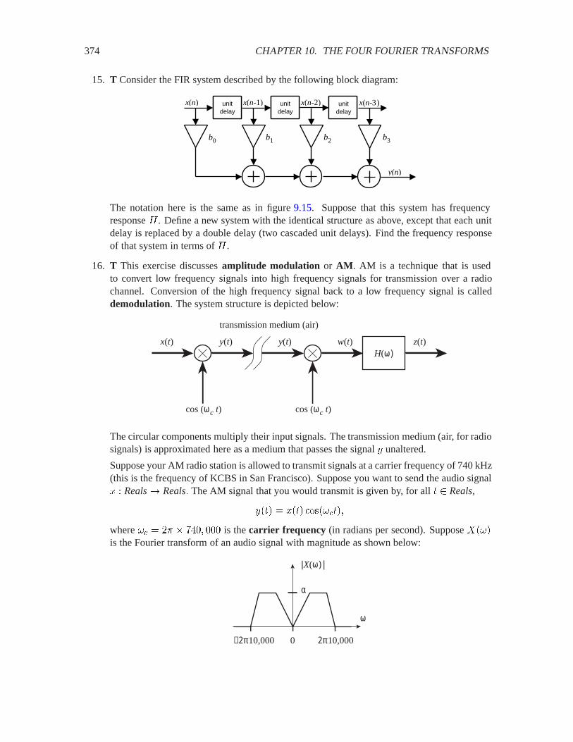
374 CHAPTER 10. THE FOUR FOURIER TRANSFORMS
15. T Consider the FIR system described by the following block diagram:
unitdelay
unitdelay
unitdelay
x(n) x(n-1) x(n-2) x(n-3)
b0
y(n)
b1 b2 b3
The notation here is the same as in figure 9.15. Suppose that this system has frequencyresponse ; . Define a new system with the identical structure as above, except that each unitdelay is replaced by a double delay (two cascaded unit delays). Find the frequency responseof that system in terms of ; .
16. T This exercise discusses amplitude modulation or AM. AM is a technique that is usedto convert low frequency signals into high frequency signals for transmission over a radiochannel. Conversion of the high frequency signal back to a low frequency signal is calleddemodulation. The system structure is depicted below:
x(t)
cos (ωc t)
transmission medium (air)
H(ω)y(t)
cos (ωc t)
y(t) w(t) z(t)
The circular components multiply their input signals. The transmission medium (air, for radiosignals) is approximated here as a medium that passes the signal � unaltered.
Suppose your AM radio station is allowed to transmit signals at a carrier frequency of 740 kHz(this is the frequency of KCBS in San Francisco). Suppose you want to send the audio signal� � Reals� Reals� The AM signal that you would transmit is given by, for all Reals,
��� � ��� ��������
where �� � �� � ��� is the carrier frequency (in radians per second). Suppose ����is the Fourier transform of an audio signal with magnitude as shown below:
|X(ω)|
ω
2π10,000
α
−2π10,000 0

10.8. SUMMARY 375
(a) Show that the Fourier transform $ of � in terms of � is
$ ��� � ���� � ��� ���� � �������
(b) Carefully sketch �$ ���� and note the important magnitudes and frequencies on yoursketch.
Note that if ���� � for ��� 2 �� � � , then $ ��� � for ���� � ����� 2�� � � . In words, if the signal � being modulated is bandlimited to less than 10kHz, then the modulated signal is bandlimited to frequencies that are withing 10 kHz ofthe carrier frequency. Thus, an AM radio station only needs to occupy 20 kHz of theradio spectrum in order to transmit audio signals up to 10 kHz.
(c) At the receiver, the problem is to recover the audio signal � from �. One way is todemodulate by multiplying � by a sinewave at the carrier frequency to obtain the signal/, where
/�� � ��� ��������
What is the Fourier transform 7 of / in terms of �? Sketch �7 ���� and note theimportant magnitudes and frequencies.
(d) After performing the demodulation of part (c), an AM receiver will filter the receivedsignal through a low-pass filter with frequency response ;��� such that ;��� � for��� � �� � � and �;���� � for ��� 2 �� � �� . Let � be the filteredsignal, as shown in the figure above. What is the Fourier transform % of �? What is therelationship between � and �?
17. T In the following parts, assume that � is a discrete-time signal given by
� � Integers� ���� � ��� � � ��� � ��� ��
and that . is an LTI system with frequency response ; given by
� � Reals� ;��� � �����
(a) Find � � DTFT��� and make a well-labeled sketch for � ���� �� in radians/sample.Check that � is periodic with period ��.
(b) Let � � .���. Find $ � DTFT���.
(c) Find � � .���.
(d) Sketch � and � and comment on what the system . does.
18. T Consider a causal discrete-time LTI system . with input � and output � such that
� � Integers� ���� � ���� � ����� �
where � Realsis a given constant such that ��� ) .
(a) Find the impulse response � of ..
(b) Find the frequency response of . by letting the input be ���� and the output be ;�������,and solving for ;���.
376 CHAPTER 10. THE FOUR FOURIER TRANSFORMS
(c) Use your results in parts (a) and (b) and the fact that the DTFT of an impulse responseis the frequency response to show that � given by
� � Integers� ���� � ��0���
has the discrete-time Fourier transform ; � DTFT��� given by
;��� �
� ������
where 0��� is the unit step, given by (2.15).
(d) Use Matlab to plot ���� and �;���� for � � ��� and � � ��. You may choose theinterval of � for your plot of �, but you should plot �;���� in the interval � ���� ��.Discuss the differences between these plots for the two different values of �.
19. T Suppose a discrete-time signal � has DTFT given by
���� � & ����>��
for some positive integer > . Note that ���� is periodic with period ��, as it must be to be aDTFT.
(a) Determine from the symmetry properties of � whether the time-domain signal � is real.
(b) Find �. Hint: Use Euler’s relation and the linearity of the DTFT.
20. T Consider a periodic continuous-time signal �with period ( and Fourier series �� Integers�Complex. Let � be another signal given by
��� � ��� ��
for some real constant � . Find the Fourier series coefficients of � in terms of those of � .
21. T Consider the continuous-time signal given by
��� ������� �
��� ��
Show that its CTFT is given by
���� �
�� if ��� � ��� if ��� 2 ��
The fact from calculus (10.5) may be useful.
22. T If � is a continuous-time signal with CTFT � , then we can define a new time-domainfunction � such that
� Reals� ��� � ����
That is, the new time domain function has the same shape as the frequency domain function� . Then the CTFT $ of � is given by
� � Reals� $ ��� � ��������That is, the frequency domain of the new function has the shape of the time domain of theold, but reversed and scaled by ��. This property is called duality because it shows that timeand frequency are interchangeable. Show that the property is true.
10.8. SUMMARY 377
23. T Use the results of exercises 21 and 22 to show that a continuous time signal � given by
��� �
����� if �� � �� if �� 2 �
where � is a positive real number, has CTFT � given by
���� � ���������
�����

378 CHAPTER 10. THE FOUR FOURIER TRANSFORMS

Chapter 11
Sampling and Reconstruction
Digital hardware, including computers, take actions in discrete steps. So they can deal with discrete-time signals, but they cannot directly handle the continuous-time signals that are prevalent in thephysical world. This chapter is about the interface between these two worlds, one continuous, theother discrete. A discrete-time signal is constructed by sampling a continuous-time signal, and acontinuous-time signal is reconstructed by interpolating a discrete-time signal.
11.1 Sampling
A sampler for complex-valued signals is a system
Sampler� � �Reals� Complex�� �Integers� Complex�� (11.1)
where is the sampling interval (it has units of seconds/sample). The system is depicted infigure 11.1. The sampling frequency or sample rate is �� � � , in units of samples/second (orsometimes, Hertz), or �� � ��� , in units radians/second. If � � Sampler� ��� then � is definedby
� � Integers� ���� � ��� �� (11.2)
y: Integers → Complexx: Reals → ComplexSamplerT
Figure 11.1: Sampler.
379
380 CHAPTER 11. SAMPLING AND RECONSTRUCTION
Basics: Units
Recall that frequency can be given with any of various units. The units of the � in(11.3) and (11.4) are Hertz, or cycles/second. In (11.3), it is sensible to give thefrequency as � � ��� , which has units of radians/second. The constant �� hasunits of radians/cycle, so the units work out. Moreover, the time argument hasunits of seconds, so the argument to the cosine function, ���, has units of radians,as expected.
In the discrete time case (11.4), it is sensible to give the frequency as ��� , whichhas units of radians/sample. The sampling interval has units of seconds/sample,so again the units work out. Moreover, the integer � has units of samples, so againthe argument to the cosine function, ���� , has units of radians, as expected.
In general, when discussing continuous-time signals and their sampled discrete-time signals, it is important to be careful and consistent in the units used, or con-siderable confusion can result. Many texts talk about normalized frequency whendiscussing discrete-time signals, by which they simply mean frequency in units ofradians/sample. This is normalized in the sense that it does not depend on thesampling interval.
11.1.1 Sampling a sinusoid
Let ��Reals� Realsbe the sinusoidal signal
� Reals� ��� � ��������� (11.3)
where � is the frequency of the sinewave in Hertz. Let � � Sampler� ���. Then
� � Integers� ���� � �������� �� (11.4)
Although this looks similar to the continuous-time sinusoid, there is a fundamental difference. Be-cause the index � is discrete, it turns out that the frequency � is indistinguishable from frequency� � �� when looking at the discrete-time signal. This phenomenon is called aliasing.
11.1.2 Aliasing
Consider another sinusoidal signal 0 given by
� Reals� 0�� � �������� �������
where � is some integer and �� � � . If � �� , then this signal is clearly different from � in(11.3). Let
/ � Sampler� �0��
11.1. SAMPLING 381
Then for all � Integers,
/��� � �������� ������ � � �������� � ����� � �������� � � �����
because �� is an integer. Thus, even though 0 �� �, Sampler� �0� � Sampler� ���. Thus, afterbeing sampled, the signals � and 0 are indistinguishable. This phenomenon is called aliasing,presumably because it implies that any discrete-time sinusoidal signal has many continuous-timeidentities (its “identity” is presumably its frequency).
Example 11.1: A typical sample rate for voice signals is �� � � samples/second,so the sampling interval is � ��� msec/sample. A continuous-time sinusoid withfrequency 440 Hz, when sampled at this rate, is indistinguishable from a continuous-time sinusoid with frequency 8,440 Hz, when sampled at this same rate.
Example 11.2: Compact discs are created by sampling audio signals at �� � ��� Hz, so the sampling interval is about � ���� -sec/sample. A continuous-time si-nusoid with frequency 440 Hz, when sampled at this rate, is indistinguishable from acontinuous-time sinusoid with frequency 44,540 Hz, when sampled at this same rate.
The frequency domain analysis of the previous chapters relied heavily on complex exponentialsignals. Recall that a cosine can be given as a sum of two complex exponentials, using Euler’srelation,
�������� � ������)$� � ����)$���
One of the complex exponentials is at frequency � , an the other is at frequency �� . Complexexponential exhibit the same aliasing behavior that we have illustrated for sinusoids.
Let ��Reals� Complexbe� Reals� ��� � ���)$�
where � is the frequency in Hertz. Let � � Sampler� ���. Then for all � in Integers,
���� � ���)$��
Consider another complex exponential signal 0,
0�� � ���) $��$���
where � is some integer. Let/ � Sampler� �0��
Then for all � Integers,
/��� � ���) $��$���� � ���)$�� ���)�$��� � ���)$�� � �����
because ���)�$��� � . Thus, as with sinusoids, when we sample a complex exponential signalwith frequency � at sample rate ��, it is indistinguishable from one at frequency � ��� (or � ����for any integer � ).
There is considerably more to this story. Mathematically, aliasing relates to the periodicity of thefrequency domain representation (the DTFT) of a discrete-time signal. We will also see that the ef-fects of aliasing on real-valued signals (like the cosine, but unlike the complex exponential) dependstrongly on the conjugate symmetry of the DTFT as well.

382 CHAPTER 11. SAMPLING AND RECONSTRUCTION
8 kHz
8 kHz
Continuous-timesignal
4 kHz
4 kHz
Frequency of the continuous-time sinusoid
Perceivedpitch
freq
uenc
y
sweep
Figure 11.2: As the frequency of a continuous signal increases beyond theNyquist frequency, the perceived pitch starts to drop.
11.1.3 Perceived pitch experiment
Consider the following experiment.1 Generate a discrete-time audio signal with an 8,000 sam-ples/second sample rate according to the formula (11.4). Let the frequency � begin at 0 Hz andsweep upwards through 4 kHz to (at least) 8 kHz. Use the audio output of a computer to listen tothe resulting sound. The result is illustrated in figure11.2. As the frequency of the continuous-timesinusoid rises, so does the perceived pitch, until the frequency reaches 4 kHz. At that point, theperceived pitch begins to fall rather than rise, even as the frequency of the continuous-time sinusoidcontinues to rise. It will fall until the frequency reaches 8 kHz, at which point no sound is heard atall (the perceived pitch is 0 Hz). Then the perceived pitch begins to rise again.
That the perceived pitch rises from 0 after the frequency � rises above 8000 Hz is not surprising. Wehave already determined that in a discrete-time signal, a frequency of � is indistinguishable from afrequency ���, assuming the sample rate is 8,000 samples/second. But why does the perceivedpitch drop when � rises above 4 kHz?
The frequency 4 kHz, ����, is called the Nyquist frequency, after Harry Nyquist, an engineer atBell Labs who, in the 1920s and 1930s, laid much of the groundwork for digital transmission ofinformation. The Nyquist frequency turns out to be a key threshold in the relationship betweendiscrete-time and continuous-time signals, more important even than the sampling frequency. In-tuitively, this is because if we sample a sinusoid with a frequency below the Nyquist frequency(below half the sampling frequency), then we take at least two samples per cycle of the sinusoid. Itshould be intuitively appealing that taking at least two samples per cycle of a sinusoid has some key
1This experiment can be performed at http://www.eecs.berkeley.edu/eal/eecs20/week13/aliasing.html. Similar exper-iments are carried out in lab C.11.
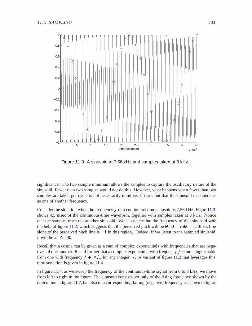
11.1. SAMPLING 383
0 0.5 1 1.5 2 2.5 3 3.5 4 4.5
x 10−3
−1
−0.8
−0.6
−0.4
−0.2
0
0.2
0.4
0.6
0.8
1
time (seconds)
Figure 11.3: A sinusoid at 7.56 kHz and samples taken at 8 kHz.
significance. The two sample minimum allows the samples to capture the oscillatory nature of thesinusoid. Fewer than two samples would not do this. However, what happens when fewer than twosamples are taken per cycle is not necessarily intuitive. It turns out that the sinusoid masqueradesas one of another frequency.
Consider the situation when the frequency � of a continuous-time sinusoid is 7,560 Hz. Figure11.3shows 4.5 msec of the continuous-time waveform, together with samples taken at 8 kHz. Noticethat the samples trace out another sinusoid. We can determine the frequency of that sinusoid withthe help of figure 11.2, which suggests that the perceived pitch will be � � �� � �� Hz (theslope of the perceived pitch line is � in this region). Indeed, if we listen to the sampled sinusoid,it will be an A-440.
Recall that a cosine can be given as a sum of complex exponentials with frequencies that are nega-tives of one another. Recall further that a complex exponential with frequency � is indistinguishablefrom one with frequency � � ���, for any integer � . A variant of figure 11.2 that leverages thisrepresentation is given in figure 11.4.
In figure 11.4, as we sweep the frequency of the continuous-time signal from 0 to 8 kHz, we movefrom left to right in the figure. The sinusoid consists not only of the rising frequency shown by thedotted line in figure 11.2, but also of a corresponding falling (negative) frequency as shown in figure
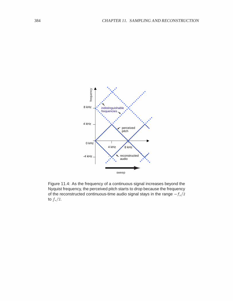
384 CHAPTER 11. SAMPLING AND RECONSTRUCTION
8 kHz
8 kHz
indistinguishablefrequencies
4 kHz
4 kHzperceivedpitch
freq
uenc
y
sweep
reconstructedaudio
0 kHz
-4 kHz
Figure 11.4: As the frequency of a continuous signal increases beyond theNyquist frequency, the perceived pitch starts to drop because the frequencyof the reconstructed continuous-time audio signal stays in the range �����to ����.
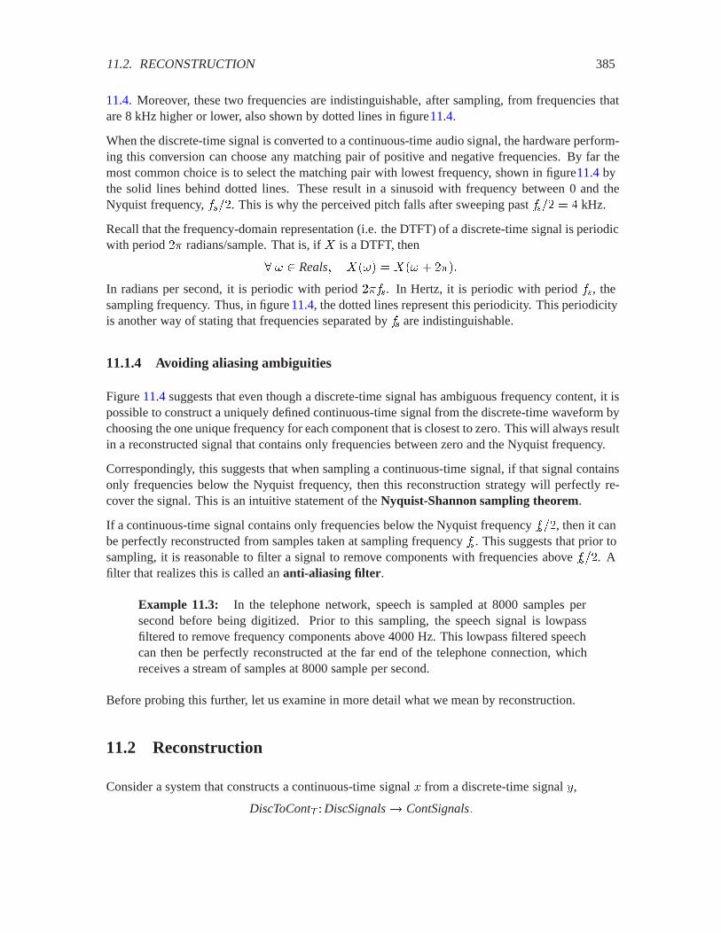
11.2. RECONSTRUCTION 385
11.4. Moreover, these two frequencies are indistinguishable, after sampling, from frequencies thatare 8 kHz higher or lower, also shown by dotted lines in figure11.4.
When the discrete-time signal is converted to a continuous-time audio signal, the hardware perform-ing this conversion can choose any matching pair of positive and negative frequencies. By far themost common choice is to select the matching pair with lowest frequency, shown in figure11.4 bythe solid lines behind dotted lines. These result in a sinusoid with frequency between 0 and theNyquist frequency, ����. This is why the perceived pitch falls after sweeping past ���� � � kHz.
Recall that the frequency-domain representation (i.e. the DTFT) of a discrete-time signal is periodicwith period �� radians/sample. That is, if � is a DTFT, then
� � Reals� ���� � ��� � ����
In radians per second, it is periodic with period ����. In Hertz, it is periodic with period ��, thesampling frequency. Thus, in figure 11.4, the dotted lines represent this periodicity. This periodicityis another way of stating that frequencies separated by �� are indistinguishable.
11.1.4 Avoiding aliasing ambiguities
Figure 11.4 suggests that even though a discrete-time signal has ambiguous frequency content, it ispossible to construct a uniquely defined continuous-time signal from the discrete-time waveform bychoosing the one unique frequency for each component that is closest to zero. This will always resultin a reconstructed signal that contains only frequencies between zero and the Nyquist frequency.
Correspondingly, this suggests that when sampling a continuous-time signal, if that signal containsonly frequencies below the Nyquist frequency, then this reconstruction strategy will perfectly re-cover the signal. This is an intuitive statement of the Nyquist-Shannon sampling theorem.
If a continuous-time signal contains only frequencies below the Nyquist frequency ����, then it canbe perfectly reconstructed from samples taken at sampling frequency ��. This suggests that prior tosampling, it is reasonable to filter a signal to remove components with frequencies above ����. Afilter that realizes this is called an anti-aliasing filter.
Example 11.3: In the telephone network, speech is sampled at 8000 samples persecond before being digitized. Prior to this sampling, the speech signal is lowpassfiltered to remove frequency components above 4000 Hz. This lowpass filtered speechcan then be perfectly reconstructed at the far end of the telephone connection, whichreceives a stream of samples at 8000 sample per second.
Before probing this further, let us examine in more detail what we mean by reconstruction.
11.2 Reconstruction
Consider a system that constructs a continuous-time signal � from a discrete-time signal �,
DiscToCont� �DiscSignals� ContSignals�

386 CHAPTER 11. SAMPLING AND RECONSTRUCTION
Probing further: Anti-Aliasing for Fonts
When rendering characters on a computer screen, it is common to use anti-aliasingto make the characters look better. Consider the two figures below:
At the left is an image of the Greek letter omega. At the right is the result ofsampling that rendition by taking only one pixel out of every 100 pixels in theoriginal (every 10-th pixel horizontally and vertically), and then rescaling the imageso it has the same size as the one on the left. The original image is discrete, and theresulting image is a smaller discrete image (this process is known as subsampling).Rendered with normal-sized pixels the character on the right looks like this:
To the discerning eye, this can be improved considerably. The problem is that thecharacter at the upper left above has hard edges, and hence high (spatial) frequen-cies. Those high frequencies result in aliasing distortion when subsampling. Toimprove the result, we first lowpass filter the character (blurring it), and then sub-sample, as shown below:
The result looks better to the discerning eye:

11.2. RECONSTRUCTION 387
y: Integers → Complex x: Reals → ComplexDiscToContT
Figure 11.5: Discrete to continuous converter.
This is illustrated in figure 11.5. Systems that carry out such ‘discrete-to-continuous’ conversioncan be realized in any number of ways. Some common examples are illustrated in figure11.6, anddefined below:
� zero-order hold: This means simply that the value of the each sample ���� is held constantfor duration , so that ��� � ���� for the time interval from � � to � �� � � , asillustrated in figure 11.6(b). Let this system be denoted
ZeroOrderHold� �DiscSignals� ContSignals�
� linear interpolation: Intuitively, this means simply that we connect the dots with straightlines. Specifically, in the time interval from � � to � �� � � , ��� has valuesthat vary along a straight line from ���� to ��� � �, as illustrated in figure11.6(c). Linearinterpolation is sometimes called first-order hold. Let this system be denoted
LinearInterpolator� �DiscSignals� ContSignals�
� ideal interpolation: It is not yet clear what this should mean, but intuitively, it should resultin a smooth curve that passes through the samples, as illustrated in figure11.6(d). We willgive a precise meaning below. Let this system be denoted
IdealInterpolator� �DiscSignals� ContSignals�
11.2.1 A model for reconstruction
A convenient mathematical model for reconstruction divides the reconstruction process into a cas-cade of two systems, as shown in figure 11.7. Thus
� � .�ImpulseGen� �����
where . is an LTI system to be determined. The first of these two subsystems,
ImpulseGen� �DiscSignals� ContSignals�
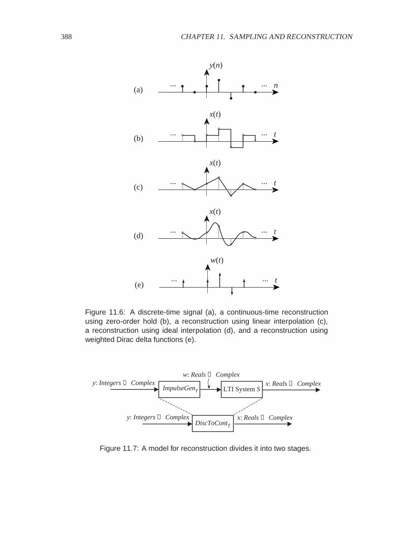
388 CHAPTER 11. SAMPLING AND RECONSTRUCTION
y(n)
n......
x(t)
t......
x(t)
t......
x(t)
t......
(a)
(b)
(c)
(d)
w(t)
t......(e)
Figure 11.6: A discrete-time signal (a), a continuous-time reconstructionusing zero-order hold (b), a reconstruction using linear interpolation (c),a reconstruction using ideal interpolation (d), and a reconstruction usingweighted Dirac delta functions (e).
y: Integers → Complex x: Reals → ComplexDiscToContT
y: Integers → ComplexImpulseGenT LTI System S
w: Reals → Complexx: Reals → Complex
Figure 11.7: A model for reconstruction divides it into two stages.
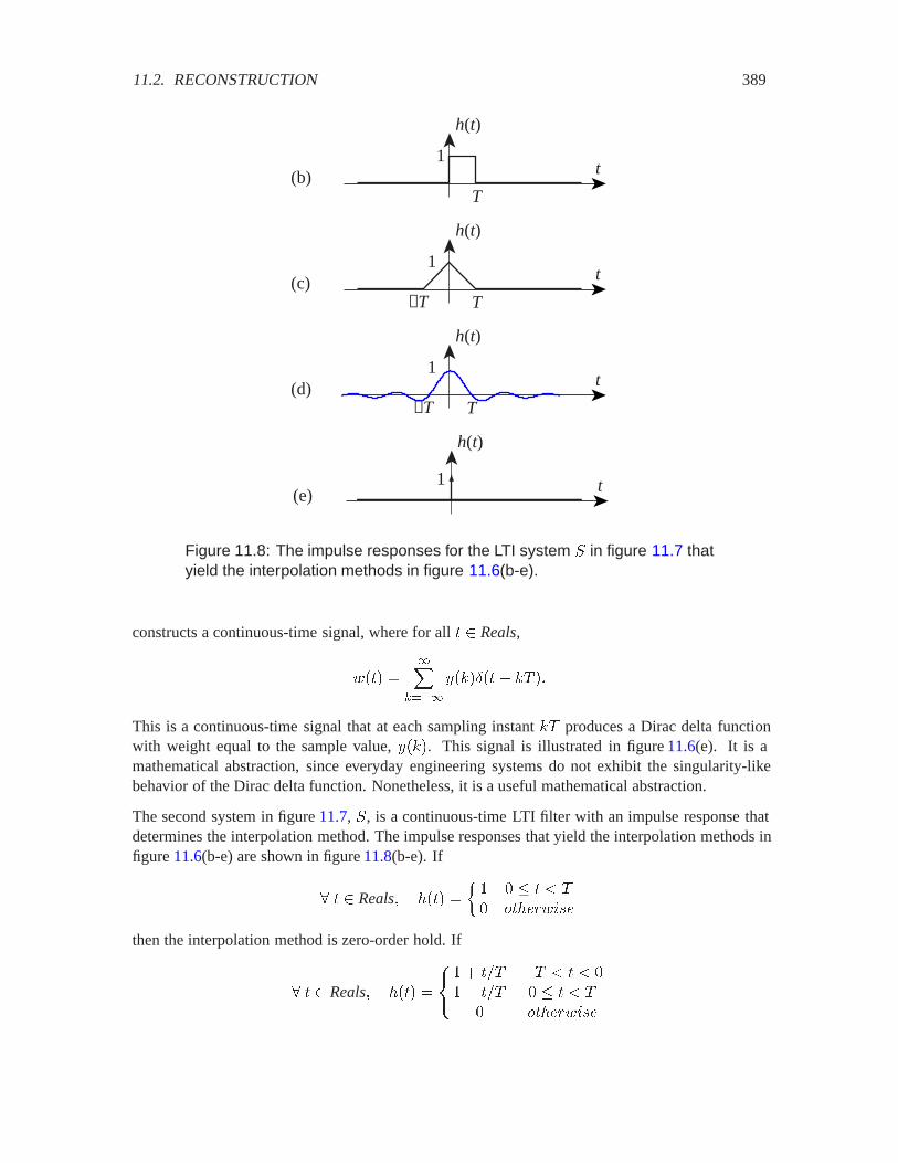
11.2. RECONSTRUCTION 389
h(t)
t(b)
(c)
(d)
h(t)
t(e)
1
T
h(t)
t1
T−T
h(t)
t1
T−T
1
Figure 11.8: The impulse responses for the LTI system . in figure 11.7 thatyield the interpolation methods in figure 11.6(b-e).
constructs a continuous-time signal, where for all Reals,
/�� ���
����
��6�� � 6 ��
This is a continuous-time signal that at each sampling instant 6 produces a Dirac delta functionwith weight equal to the sample value, ��6�. This signal is illustrated in figure 11.6(e). It is amathematical abstraction, since everyday engineering systems do not exhibit the singularity-likebehavior of the Dirac delta function. Nonetheless, it is a useful mathematical abstraction.
The second system in figure 11.7, ., is a continuous-time LTI filter with an impulse response thatdetermines the interpolation method. The impulse responses that yield the interpolation methods infigure 11.6(b-e) are shown in figure 11.8(b-e). If
� Reals� ��� �
� � ) 4���/&��
then the interpolation method is zero-order hold. If
� Reals� ��� �
�� � � � ) ) � � � )
4���/&��

390 CHAPTER 11. SAMPLING AND RECONSTRUCTION
then the interpolation method is linear. If the impulse response is
� Reals� ��� ������� �
��
then the interpolation method is ideal. The above impulse response is called a sinc function, and itsFourier transform, from table 10.4, is given by
� � Reals� ���� �
� if ��� � �� otherwise
Notice that the Fourier transform is zero at all frequencies above �� radians/second, or ���� Hz,the Nyquist frequency. It is this characteristic that makes it ideal. It precisely performs the strategyillustrated in figure 11.4, where among all indistinguishable frequencies we select the ones between����� and ����.
If we let Sinc� denote the LTI system . when the impulse response is a sinc function, then
IdealInterpolator� � Sinc� Æ ImpulseGen� �
In practice, ideal interpolation is difficult to accomplish. From the expression for the sinc functionwe can understand why. First, this impulse response is not causal. Second, it is infinite in extent.More importantly, its magnitude decreases rather slowly as increases or decreases (proportional to� only). Thus, truncating it at finite length leads to substantial errors.
If the impulse response of . is��� � ���
where Æ is the Dirac delta function, then the system . is a pass-through system, and the reconstruc-tion consists of weighted delta functions.
11.3 The Nyquist-Shannon sampling theorem
We can now give a precise statement of the Nyquist-Shannon sampling theorem:
If � is a continuous-time signal with Fourier transform � and if ���� is zerooutside the range ��� ) � ) �� radians/second, then
� � IdealInterpolator� �Sampler� �����
We can state this theorem slightly differently. Suppose � is a continuous-time signal with no fre-quency larger than some �� Hertz. Then � can be recovered from its samples if �� ) ����, theNyquist frequency.

11.3. THE NYQUIST-SHANNON SAMPLING THEOREM 391
Probing further: Sampling
We can construct a mathematical model for sampling by using Dirac delta func-tions. Define a pulse stream by
� Reals� (�� ���
����
�� 6 ��
Consider a continuous-time signal � that we wish to sample with sampling period . That is, we define ���� � ��� �� Construct first an intermediate continuous-time signal /�� � ���(��� We can show that the CTFT of / is equal to the DTFTof �. This gives us a way to relate the CTFT of � to the DTFT of its samples �.Recall that multiplication in the time domain results in convolution in the frequencydomain (see table 10.9), so
7 ��� �
������ � � ��� �
��
����
����� �� � �����
It can be shown (see box on page 392 that the CTFT of (�� is
� ��� ���
������
�� � 6��
��
so
7 ��� �
��
����
������
������
�� ��� 6��
���
�
������
����
������ � �� 6��
���
�
������
��� � 6��
�
where the last equality follows from the sifting property (9.11). The next step is toshow that
$ ��� � 7 ��� ��
We leave this as an exercise. From this, the basic Nyquist-Shannon result follows,
$ ��� �
������
�
�� � ��6
��
This relates the CTFT � of the signal being sampled � to the DTFT $ of thediscrete-time result �.

392 CHAPTER 11. SAMPLING AND RECONSTRUCTION
Probing further: Impulse Trains
Consider a signal ( consisting of periodically repeated Dirac delta functions withperiod ,
� Reals� (�� ���
����
�� 6 ��
This signal has the Fourier series expansion
� Reals� (�� ���
����
�������
where the fundamental frequency is �� � ��� . This can be verified by applyingthe formula from table 10.5. That formula, however, gives an integration rangeof 0 to the period, which in this case is . This integral covers one period of theperiodic signal, but starts and ends on a delta function in (. To avoid the resultantmathematical subtleties, we can integrate from��� to ��, getting Fourier seriescoefficients
�' Integers� �� �
��������
�� ������
� � 6 �
�� ��������
The integral is now over a range that includes only one of the delta functions. Thekernel of the integral is zero except when � , so by the sifting rule, the integralevaluates to 1. Thus, all Fourier series coefficients are �� � � . Using therelationship between the Fourier series and the Fourier Transform of a periodicsignal (from section 10.6.3), we can write the continuous-time Fourier transform of( as
� � Reals� � ��� ���
������
Æ
�� � ��
6
��
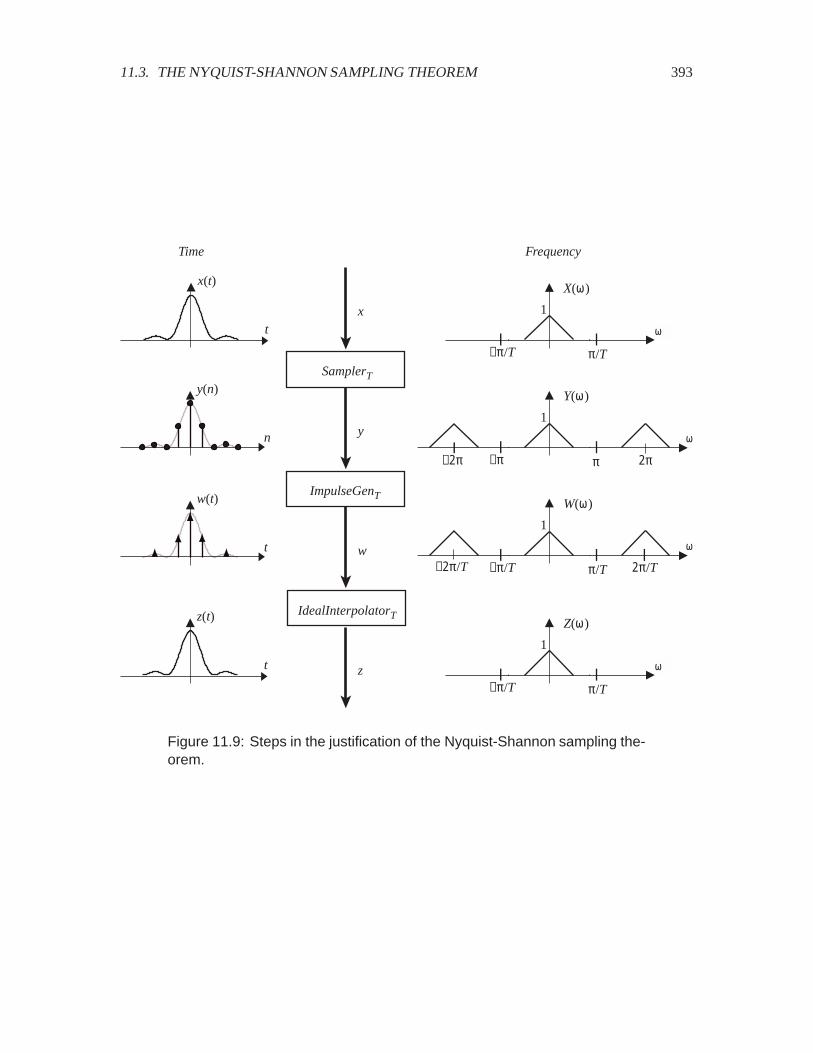
11.3. THE NYQUIST-SHANNON SAMPLING THEOREM 393
ω
X(ω)
1
π/T−π/T
t
x(t)
SamplerT
ImpulseGenT
n
y(n)
ω
Y(ω)
1
π−π
ω
W(ω)
1
π/T−π/T
t
w(t)
−2π
−2π/T
2π
2π/T
IdealInterpolatorT
t
z(t)
ω
Z(ω)
1
π/T−π/T
x
y
w
z
Time Frequency
Figure 11.9: Steps in the justification of the Nyquist-Shannon sampling the-orem.

394 CHAPTER 11. SAMPLING AND RECONSTRUCTION
ω
π−πω
X(ω)
Y(ω)
1
π/T−π/T
1/T......
3π−3π
Figure 11.10: Relationship between the CTFT of a continuous-time signaland the DTFT of its discrete-time samples. The DTFT is the sum of theCTFT and its copies shifted by multiples of ��� , the sampling frequencyin radians per second. The frequency axis is also normalized.
A formal proof of this theorem involves some technical difficulties (it was first given by ClaudeShannon of Bell Labs in the late 1940s). But we can get the idea from the following three-stepargument (see figure 11.9).
Step 1. Let � be a continuous-time signal with Fourier transform � . At this point we do not requirethat ���� be zero outside the range ��� ) � ) �� . We sample � with sampling interval toget the discrete-time signal
� � Sampler� ����
It can be shown (see box on page 391 ) that the DTFT of � is related to the CTFT of � by
$ ��� � ��
������
�(�� � �)�
�
)�
This important relation says that the DTFT $ of � is the sum of the CTFT � with copies of itshifted by multiples of ��� . Also, the frequency axis is normalized by dividing � by . There aretwo cases to consider, depending on whether the shifted copies overlap.
First, if ���� � outside the range ��� ) � ) �� , then the copies will not overlap, and inthe range �� ) � ) �,
$ ��� �
�
��
�� (11.5)
In this range of frequencies, $ has the same shape as � , scaled by � . This relationship between� and $ is illustrated in figure 11.10, where � is drawn with a triangular shape.
In the second case, illustrated in figure 11.11, � does have non-zero frequency components higherthan �� . Notice that in the sampled signal, the frequencies in the vicinity of � are distorted by theoverlapping of frequency components above and below �� in the original signal. This distortionis called aliasing distortion.
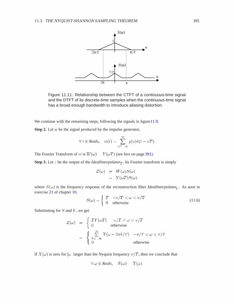
11.3. THE NYQUIST-SHANNON SAMPLING THEOREM 395
ω
ω
−π π
X(ω)
Y(ω)
1
π/T−π/T
1/T
Figure 11.11: Relationship between the CTFT of a continuous-time signaland the DTFT of its discrete-time samples when the continuous-time signalhas a broad enough bandwidth to introduce aliasing distortion.
We continue with the remaining steps, following the signals in figure11.9.
Step 2. Let / be the signal produced by the impulse generator,
� Reals� /�� ���
����
������ � ��
The Fourier Transform of / is 7 ��� � $ �� � (see box on page 391).
Step 3. Let � be the output of the IdealInterpolator� . Its Fourier transform is simply
%��� � 7 ���.���
� $ �� �.����
where .��� is the frequency response of the reconstruction filter IdealInterpolator� . As seen inexercise 21 of chapter 10,
.��� �
� ��� ) � ) �� otherwise
(11.6)
Substituting for . and $ , we get
%��� �
�$ �� � ��� ) � ) �� otherwise
�
��
������
��� � ��6� � ��� ) � ) ��
otherwise
If ���� is zero for ��� larger than the Nyquist frequency �� , then we conclude that
� � Reals� %��� � �����
396 CHAPTER 11. SAMPLING AND RECONSTRUCTION
That is, / is identical to �. This proves the Nyquist-Shannon result.
However, if ���� does have non-zero values for some ��� larger than the Nyquist frequency, then� will be different from �, as illustrated in figure 11.11.
11.4 Summary
The acts of sampling and reconstructing a continuous-time signal bridge the continuous-time worldwith the discrete computational world. The periodicity of frequencies in the discrete world impliesthat for each discrete-time sinusoidal signal, there are multiple corresponding discrete-time fre-quencies. These frequencies are aliases of one another. When a signal is sampled, these frequenciesbecome indistinguishable, and aliasing distortion may result. The Nyquist-Shannon sampling theo-rem gives a simple condition under which aliasing distortion is avoided. Specifically, if the signalcontains no sinusoidal components with frequencies higher than half the sampling frequency, thenthere will be no aliasing distortion. Half the sampling frequency is called the Nyquist frequencybecause of this key result.
Exercises
Each problem is annotated with the letter E, T, C which stands for exercise, requires some thought,requires some conceptualization. Problems labeled E are usually mechanical, those labeled T re-quire a plan of attack, those labeled C usually have more than one defensible answer.
1. E Consider the continuous-time signal
��� � ������ � ������� � ��������
(a) Find the fundamental frequency. Give the units.
(b) Find the Fourier series coefficients ��� ��� and <�� <�� .(c) Let � be the result of sampling this signal with sampling frequency 10 Hz. Find the
fundamental frequency for �, and give the units.
(d) For the same �, find the discrete-time Fourier series coefficients, ��� ��� and <�� .(e) Find
/ � IdealInterpolator� �Sampler� ����
for � � seconds.
(f) Is there any aliasing distortion caused by sampling at 10 Hz? If there is, describe thealiasing distortion in words.
(g) Give the smallest sampling frequency that avoids aliasing distortion.
2. E Verify that Sampler� defined by (11.1) and (11.2) is linear but not time invariant.

11.4. SUMMARY 397
3. E A real-valued sinusoidal signal with a negative frequency is always exactly equal to anothersinusoid with positive frequency. Consider a real-valued sinusoid with a negative frequency��� Hz,
���� � ���������� � <��
Find a positive frequency � and phase # such that
���� � �������� � #��
4. T Consider a continuous-time signal � where for all Reals,
��� ���
����
��� 6��
where
��� �
� � ) �� 4���/&��
�
(a) Is ��� periodic? If so, what is the period?
(b) Suppose that � . Give a simple expression for � � Sampler� ���.
(c) Suppose that � ��. Give a simple expression for � � Sampler� ��� and � �IdealInterpolator� �Sampler� ����.
(d) Find an upper bound for (in seconds) such that � � IdealInterpolator� �Sampler� ����,or argue that no value of makes this assertion true.
5. T Consider a continuous-time signal � with the following finite Fourier series expansion,
� Reals� ��� ��
���
����6���
where �� � ��� radians/second.
(a) Give an upper bound on (in seconds) such that � � IdealInterpolator� �Sampler� ����.
(b) Suppose that � � seconds. Give a simple expression for � � Sampler� ���.
(c) For the same � � seconds, give a simple expression for
/ � IdealInterpolator� �Sampler� �����
6. T Consider a continuous-time audio signal � with CTFT shown in figure 11.12. Note that itcontains no frequencies beyond 10 kHz. Suppose it is sampled at 40 kHz to yield a signal thatwe will call ��. Let �� be the DTFT of ��.
(a) Sketch ������� and carefully mark the magnitudes and frequencies.
(b) Suppose � is sampled at 20,000 samples/second. Let ��� be the resulting sampled signaland ��� its DTFT. Sketch and compare ��� and ��.
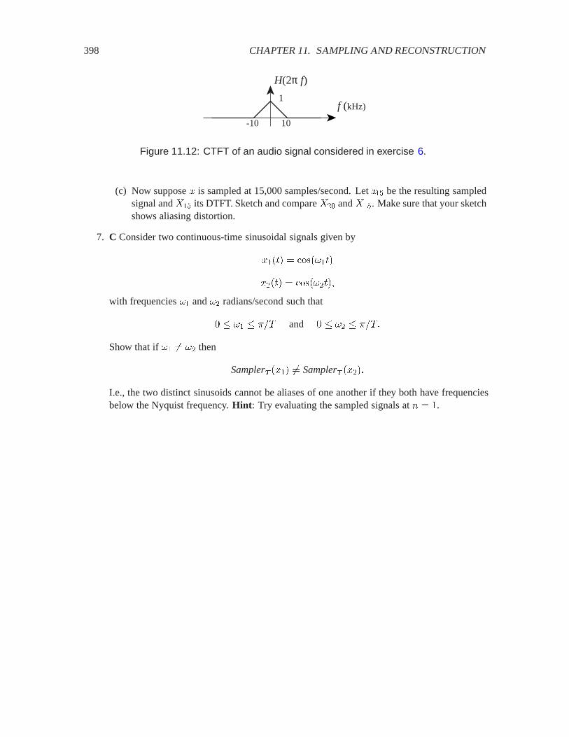
398 CHAPTER 11. SAMPLING AND RECONSTRUCTION
H(2π f)
f (kHz)1
10 -10
Figure 11.12: CTFT of an audio signal considered in exercise 6.
(c) Now suppose � is sampled at 15,000 samples/second. Let ��� be the resulting sampledsignal and ��� its DTFT. Sketch and compare ��� and ���. Make sure that your sketchshows aliasing distortion.
7. C Consider two continuous-time sinusoidal signals given by
���� � �������
���� � ��������
with frequencies �� and �� radians/second such that
� �� � �� and � �� � ���
Show that if �� �� �� then
Sampler� ���� �� Sampler� �����
I.e., the two distinct sinusoids cannot be aliases of one another if they both have frequenciesbelow the Nyquist frequency. Hint: Try evaluating the sampled signals at � � .
Chapter 12
Stability
The four Fourier transforms prove to be useful tools for analyzing signals and systems. When asystem is LTI, it is characterized by its frequency response ; , and its input � and output � arerelated simply by
�� Reals� $ ��� � ;��������
where $ is the Fourier transform of �, and � is the Fourier transform of �.
However, there is a lurking problem that we have ignored. Any of the three Fourier transforms,� , $ , or ; , may not exist. Suppose for example that � is a discrete-time signal. Then its Fouriertransform (the DTFT) is given by
� � Reals� ���� ���
����
���������� (12.1)
This is an infinite sum, properly viewed as the limit
� � Reals� ���� � !����
������
���������� (12.2)
As with all such limits, there is a risk that it does not exist. If the limit does not exist for any� Reals, then the Fourier transform becomes mathematically treacherous at best (involving, forexample, Dirac delta functions), and mathematical nonsense at worst.
Example 12.1: Consider the sequence
���� �
�� � � ����� � 2
�
where � 2 is a constant. Plugging into (12.1), the Fourier transform should be
� � Reals� ���� ������
����������
399
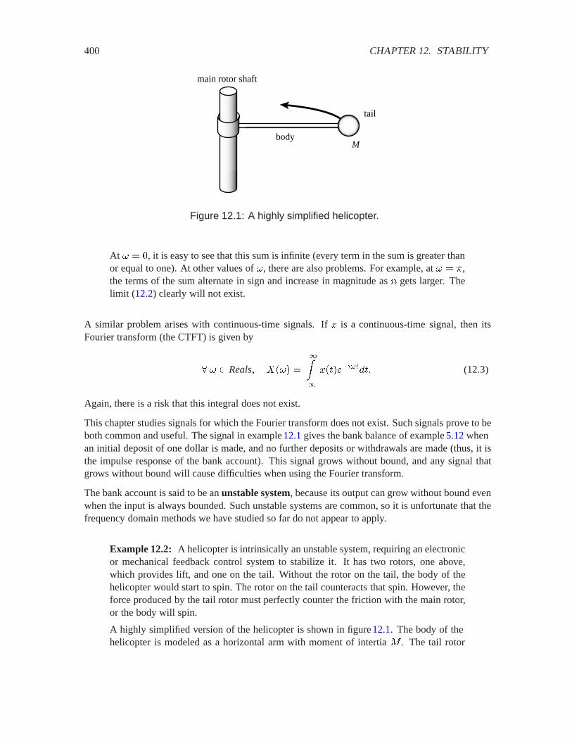
400 CHAPTER 12. STABILITY
Mbody
tail
main rotor shaft
Figure 12.1: A highly simplified helicopter.
At � � , it is easy to see that this sum is infinite (every term in the sum is greater thanor equal to one). At other values of �, there are also problems. For example, at � � �,the terms of the sum alternate in sign and increase in magnitude as � gets larger. Thelimit (12.2) clearly will not exist.
A similar problem arises with continuous-time signals. If � is a continuous-time signal, then itsFourier transform (the CTFT) is given by
� � Reals� ���� �
����
���������� (12.3)
Again, there is a risk that this integral does not exist.
This chapter studies signals for which the Fourier transform does not exist. Such signals prove to beboth common and useful. The signal in example 12.1 gives the bank balance of example 5.12 whenan initial deposit of one dollar is made, and no further deposits or withdrawals are made (thus, it isthe impulse response of the bank account). This signal grows without bound, and any signal thatgrows without bound will cause difficulties when using the Fourier transform.
The bank account is said to be an unstable system, because its output can grow without bound evenwhen the input is always bounded. Such unstable systems are common, so it is unfortunate that thefrequency domain methods we have studied so far do not appear to apply.
Example 12.2: A helicopter is intrinsically an unstable system, requiring an electronicor mechanical feedback control system to stabilize it. It has two rotors, one above,which provides lift, and one on the tail. Without the rotor on the tail, the body of thehelicopter would start to spin. The rotor on the tail counteracts that spin. However, theforce produced by the tail rotor must perfectly counter the friction with the main rotor,or the body will spin.
A highly simplified version of the helicopter is shown in figure 12.1. The body of thehelicopter is modeled as a horizontal arm with moment of intertia 3 . The tail rotor
401
goes on the end of this arm. The body of the helicopter rotates freely around the mainrotor shaft. Friction with the main rotor will tend to cause it to rotate by applying atorque as suggested by the curved arrow. The tail rotor will have to counter that torqueto keep the body of the helicopter from spinning.
Let the input � to the system be the net torque on the tail of the helicopter, as a functionof time. That is, at time , ��� is the difference between the frictional torque exertedby the main rotor shaft and the counteracting torque exerted by the tail rotor. Let theoutput � be the velocity of rotation of the body. From basic physics, torque equalsmoment of inertial times rotational acceleration. The rotational acceleration is ��, thederivative of �, so
���� � ����3�
Integrating both sides, assuming that the initial velocity of rotation is zero, we get theoutput as a function of the input,
� Reals� ��� �
3
���
�������
It is now easy to see that this system is unstable. Let the input be � � 0, where 0 is theunit step, given by
� Reals� 0�� �
�� ) � �
� (12.4)
This input is clearly bounded. It never exceeds one in magnitude. However, the outputgrows without bound.
In practice, a helicopter uses a feedback system to determine how much torque to applyat the tail rotor to keep the body of the helicopter straight. We will see how to do thisin chapter 14.
In this chapter we develop the basics of modeling unstable systems in the frequency domain. Wedefine two new transforms, called the Z transform and Laplace transform. The Z transformis a generalization of the DTFT and applies to discrete-time signals. The Laplace transform is ageneralization of the CTFT and applies to continuous-time signals. These generalizations supportfrequency-domain analysis of signals that do not have a Fourier transform, and thus allow analysisof unstable systems.
In particular, let �� denote the Laplace or Z transform of �, depending on whether it is a continuousor discrete-time signal. Then the Laplace or Z transform of the output of an LTI system is given by�$ � �; �� , where �; is the Laplace or Z transform of the impulse response. This relation applieseven when the system is unstable. Thus, these transforms take the place of the Fourier transformwhen the Fourier transform cannot be used. �; is called the transfer function of the LTI system,and it is a generalization of the frequency response.
402 CHAPTER 12. STABILITY
12.1 Boundedness and stability
In this section, we identify a simple condition for the existence of the DTFT, which is that the signalbe absolutely summable. We then define a stable system and show that an LTI system is stable ifand only if its impulse response is absolutely summable. Continuous-time signals are slightly morecomplicated, requiring slightly more than that they be absolutely integrable. The conditions for theexistence of the CTFT are called the Dirichlet conditions, and once again, if the impulse responseof an LTI system satisfies these conditions, then it is stable.
12.1.1 Absolutely summable and absolutely integrable
A discrete-time signal � is said to be absolutely summable if
������
������
exists and is finite. The “absolutely” in “absolutely summable” refers to the absolute value (ormagnitude) in the summation. The sum is said to converge absolutely. The following simple factgives a condition for the existence of the DTFT:
If a discrete-time signal � is absolutely summable, then its DTFT exists and is finitefor all �.
To see that this is true, note that the DTFT exists and is finite if and only if
� � Reals� ������ �#####
������
���������
#####exists and is finite. But #####
������
���������
##### ���
����
����������� (12.5)
���
����
������ ������� (12.6)
���
����
������� (12.7)
This follows from the following facts about complex (or real) numbers:
��� �� � ���� ����which is known as the triangle inequality (and generalizes to infinite sums),
���� � ��� ����
12.1. BOUNDEDNESS AND STABILITY 403
and� # Reals� ���*� � �
We can conclude from (12.5) that
� � Reals� ������ ���
����
�������
This means that if � is absolutely summable, then the DTFT exists and is finite. It follows from thefact that if a sum converges absolutely, then it also converges (without the absolute value).
A continuous-time signal � is said to be absolutely integrable if
����
������
exists and is finite. A similar argument to that above (with summations replaced by integrals)suggests that if a continuous-time signal � is absolutely integrable, then its CTFT should exist and befinite for all �. However, caution is in order. Integrals are more complicated than summations, andwe need some additional conditions to ensure that the integral is well defined. We can use essentiallythe same conditions given on page 236 for the convergence of the continuous-time Fourier series.These are called the Dirichlet conditions, and require three things:
� � is absolutely integrable;
� in any finite interval, � is of bounded variation, meaning that there are no more than a finitenumber of maxima or minima; and
� in any finite interval, � is continuous at all but a finite number of points.
Most any signal of practical engineering importance satisfies the last two conditions, so the impor-tant condition is that it be absolutely integrable. We will henceforth assume without comment thatall continuous-time signals satisfy the last two conditions, so the only important condition becomesthe first one. Under this assumption, the following simple fact gives a condition for the existence ofthe CTFT:
An absolutely integrable continuous-time signal � has a CTFT � , and its CTFT���� is finite for all � Reals.
12.1.2 Stability
A system is said to be bounded-input bounded-output stable (BIBO stable or just stable) if theoutput signal is bounded for all input signals that are bounded.

404 CHAPTER 12. STABILITY
Consider a discrete-time system with input � and output �. What it means for the input to bebounded is that there is a real number 3 ) � such that ���6�� � 3 for all 6 Integers. What itmeans for the output to be bounded is that there is a real number � )� such that ������ � � forall � Integers. The system is stable if for any bounded input with bound 3 , there is some bound� on the output.
Consider a discrete-time LTI system with impulse response �. The output � corresponding to theinput � is given by the convolution sum,
�� Integers� ���� � �� � ����� ���
����
��'�����'�� (12.8)
Suppose that the input � is bounded with bound 3 . Then, applying the triangle inequality, we seethat
������ ���
����
���'������ �'�� �3��
����
���'���
Thus, if the impulse response is absolutely summable, then the output is bounded with bound
� � 3��
����
���'���
Thus, if the impulse response of an LTI system is absolutely summable, then the system is stable.The converse is also true, but more difficult to show. That is, if the system is stable, then theimpulse response is absolutely summable (see box on page 405). The same argument applies forcontinuous-time signals, so in summary:
A discrete-time LTI system is stable if and only if its impulse response is abso-lutely summable. A continuous-time LTI system is stable if and only if its impulseresponse is absolutely integrable.
The following example makes use of the geometric series identity, valid for any real or complex� where ��� ) ,
�����
�� �
� �� (12.9)
To verify this identity, just multiply both sides by � � to get
�����
�� � ���
���
�� � �
This can be written
�� ���
���
�� ���
���
�� � �
Now note that �� � and that the two sums are identical. Since ��� ) , the sums converge, andhence they cancel, so the identity is true.

12.1. BOUNDEDNESS AND STABILITY 405
Probing further: Stable systems and their impulse response
Consider a discrete-time LTI system with real-valued impulse response �. In thisbox, we show that if the system is stable, then its impulse response is absolutelysummable. To show this, we show the contrapositive.a That is, we show that if theimpulse response is not absolutely summable, then the system is not stable. To dothis, suppose that the impulse response is not absolutely summable. That is, thesum
������
������
is not bounded. To show that the system is not stable, we need only to find onebounded input for which the output either does not exist or is not bounded. Suchan input is given by
� � Integers� ���� �
��������������� ���� �� � ���� �
This input is clearly bounded, with bound 3 � . Plugging this input into theconvolution sum (12.8) and evaluating at � � we get
��� ���
����
��'����'�
���
����
���'�������'��
���
����
���'���
where the last step follows from the fact that for real-valued ��'�, ���'��� ����'���. But since the impulse response is not absolutely summable, ��� does notexist or is not finite, so the system is not stable.
A nearly identical argument works for continuous-time systems.
aThe contrapositive of a statement “if p then q” is “if not q then not p.” The contrapositive is trueif and only if the original statement is true.
406 CHAPTER 12. STABILITY
Example 12.3: As in example 12.1, the impulse response of the bank account ofexample 5.12 is
���� �
�� � � ����� � 2
�
where � 2 is a constant that reflects the interest rate. This impulse response is notabsolutely summable, so this system is not stable. A system with the same impulseresponse, but where ) � ) , however, would be stable, as is easily verified using(12.9). To use this identity, note that
������
������ ������
����
���
���
��
�
� ��
where the second step results from a change of variables, letting ' � �� .
Example 12.4: Consider a continuous-time LTI system with impulse response
� Reals� ��� � ��0���
where � 2 is a real number and 0 is the unit step, given by (12.4). To determinewhether this system is stable, we need to determine whether the impulse response isabsolutely integrable. That is, we need to determine whether the following integralexists and is finite,
����
���0�����
Since � 2 and 0 is the unit step, this simplifies to���
����
From calculus, we know that this integral is infinite if � � , so the system is unstableif � � . The integral is finite if ) � ) and is equal to
���
��� � �� !�����
Thus, the system is stable if ) � ) .
As we see, when all pertinent signals are absolutely summable (or absolutely integrable), then wecan use Fourier transform techniques with confidence. However, many useful signals do not fall inthis category (the unit step and sinusoidal signals, for example). Moreover, many useful systemshave impulse responses that are not absolutely summable (or absolutely integrable). Fortunately,we can generalize the DTFT and CTFT to get the Z transform and Laplace transform, which easilyhandle signals that are not absolutely summable.

12.2. THE Z TRANSFORM 407
12.2 The Z transform
Consider a discrete-time signal � that is not absolutely summable. Consider the scaled signal �!given by
� � Integers� �!��� � �������� (12.10)
for some real number � � . Often, this signal is absolutely summable when � is chosen appropri-ately. This new signal, therefore, will have a DTFT, even if � does not.
Example 12.5: Continuing with example 12.3, the impulse response of the bankaccount is
���� �
�� � � ����� � 2
�
where � 2 . This system is not stable. However, the scaled signal
�!��� � �������
is absolutely summable if � 2 �. Its DTFT is
�� 2 ���� Reals� ;!��� ���
����
��'���������
���
���
������������
������
������������
� �������������
������������
���������
� ����������
The second step is by change of variables, � � ' � , and the final step applies thegeometric series identity (12.9).
In general, the DTFT of the scaled signal �! in (12.10) is
� � Reals� �!��� ���
����
��'����������
Notice that this is a function not just of �, but also of �, and in fact, we are only sure it is valid forvalues of � that yield an absolutely summable signal �! . If we define the complex number
� � ����
408 CHAPTER 12. STABILITY
then we can write this DTFT as
� � RoC���� ����� ���
������'����� (12.11)
where �� is a function called the Z transform of �,
���RoC���� Complex
where RoC��� � Complexis given by
RoC��� � �� � ���� Complex� ������� is absolutely summable. (12.12)
The term RoCis shorthand for region of convergence.
Example 12.6: Continuing example 12.5, we can recognize from the form of ;!���that the Z transform of the impulse response � is
� � RoC���� �;��� ����
� �����
� � ��
where the last step is the result of multiplying top and bottom by �. The RoCis
RoC��� � �� � ���� Complex� � 2 �
The Z tranform �; of the impulse response � of an LTI system is called the transfer function of thesystem.
12.2.1 Structure of the region of convergence
When a signal has a Fourier transform, then knowing the Fourier transform is equivalent to knowingthe signal. The signal can be obtained from its Fourier transform, and the Fourier transform can beobtained from the signal. The same is true of a Z transform, but there is a complication. The Ztransform is a function ���RoC� Complex, and it is necessary to know the set RoC to know thefunction �� . The region of convergence is a critical part of the Z transform. We will see that verydifferent signals can have very similar Z transforms that differ only in the region of convergence.
Given a discrete-time signal �, RoC��� is defined to be the set of all complex numbers � � ���� forwhich the following series converges:
������
���'������
Notice that if this series converges, then so does
������
���'�����

12.2. THE Z TRANSFORM 409
Re z
Im zIm z
Re z
Im z
causal or right sided
Re z
anti-causaltwo-sided
RoC RoCRoC
(a) (b) (c)
Figure 12.2: Three possible structures for the region of convergence of a Ztransform.
for any complex number � with magnitude �. This is because
���'����� � ���'���������� � ���'�� ����� ������� � ���'�� ������
Thus, the set RoCcould equally well be defined to be the set of all complex numbers � such that������� is absolutely summable.
Notice that whether this series converges depends only on �, the magnitude of the complex number� � ���� , and not on �, its angle. Thus, if any point � � ���� is in the set RoC, then all points ��
with the same magnitude are also in RoC. This implies that the set RoC, a subset of Complex, willhave circular symmetry.
The set RoCturns out to have even more structure. There are only three possible patterns, illustratedby the shaded areas in figure 12.2. Each figure illustrates the complex plane, and the shaded areais a region of convergence. Each possibility has circular symmetry, in that whether a point is in theRoCdepends only on its magnitude.
Figure 12.2(a) shows the RoCof a causal signal. A discrete-time signal � is causal if ���� � forall � ) . The RoCis the set of complex numbers � � ���� where following series converges:
������
���'������
But if � is causal, then��
����
���'����� ���
���
���'������
If this series converges for some given �, then it must also converge for any "� 2 � (because for all' � , "��� ) ���. Thus, if � RoC, then the RoCmust include all points in the complex planeon the circle passing through � and every point outside that circle.
Note further that not only must the RoC include every point outside the circle, but the series mustalso converge in the limit as � goes to infinity. Thus, for example, ;��� � � cannot be the Ztransform of a causal signal because its RoC cannot possibly include infinity (;��� is not finitethere).
410 CHAPTER 12. STABILITY
Figure 12.2(c) shows the RoCof an anti-causal signal. A discrete-time signal � is anti-causal if���� � for all � 2 . By a similar argument, if � RoC, then the RoCmust include all points inthe complex plane on the circle passing through � and every point inside that circle.
Figure 12.2(b) shows the RoCof a signal that is neither causal nor anti-causal. Such a signal is calleda two-sided signal. Such a signal can always be expressed as a sum of a causal signal and an anti-causal signal. The RoCis the intersection of the regions of convergence for these two components.To see this, just note that the RoC is the set of complex numbers � � ���� where following seriesconverges:
������
���'����� ����
����
���'��������
���
���'������
The first sum on the right corresponds to an anti-causal signal, and the second sum on the right to acausal signal. For this series to converge, both sums must converge. Thus, for a two-sided signal,the RoChas a ring structure.
Example 12.7: Consider the discrete-time unit step signal 0, given by
0��� �
�� � ) � � �
� (12.13)
The Z transform is, using geometric series identity (12.9),
�B��� ���
����
0�'���� ���
���
��� �
� ����
�
� � �
with domain
RoC�0� � �� Complex���
���
����� )� � �� � ��� 2 �
This region of convergence has the structure of figure12.2(a), where the dashed circlehas radius one (that circle is called the unit circle). Indeed, this signal is causal, so thisstructure makes sense.
Example 12.8: The signal " given by
"��� �
��� � ) � � �
�
has Z transform
�E ��� ���
����
"�'���� � ���
����
��� � �������
�� ��
� � �
with domain
RoC�"� � �� Complex���
����
����� )� � �� � ��� ) �
This region of convergence has the structure of figure12.2(c), where the dashed circleis again the unit circle. Indeed, this signal is anti-causal, so this structure makes sense.
12.2. THE Z TRANSFORM 411
Notice that although the Z transform �B of 0 and �E of " have the samealgebraic form, namely,����� �, they are differentfunctions, because their domains are different. Thus the Z transform ofa signal comprises both the algebraic form of the Z transform as well as its RoC.
A right-sided signal � is where for some integer � ,
���� � � � � ) ��
Of course, if � � , then this signal is also causal. However, if � ) , then the signal is two sided.Suppose � ) . Then we can write the Z transform of � as
������
���'����� ����
���
���'��������
���
���'������
The left summation on the right side is finite, and each term is finite for all � Complex, so thereforeit converges for all � Complex. Thus, the region of convergence is determined entirely by the rightsummation, which is the Z transform of the causal part of �. Thus, the region of convergence ofa right-sided signal has the same form as that of a causal sequence, as shown in figure 12.2(a).(However, if the signal is not causal, the Z transform does not converge at infinity.)
A left-sided signal � is where for some integer � ,
���� � � � � 2 ��
Of course, if � � , then this signal is also anti-causal. However, if � 2 , then the signal is twosided. Suppose � 2 . Then we can write the Z transform of � as
������
���'����� ���
����
���'��������
���
���'������
The right summation is finite, and therefore converges for all � Complexexcept � � , wherethe individual terms of the sum are not finite. Thus, the region of convergence is that of the leftsummation, except for the point � � . Thus, the region of convergence of a left-sided signal hasthe same form as that of an anti-causal sequence, as shown in figure12.2(c), except that the origin(� � ) is excluded. This, of course, is simply the structure of 12.2(b) where the inner circle haszero radius.
Some signals have no meaningful Z transform.
Example 12.9: The signal � with ���� � , for all �, does not have a Z transform.We can write � � 0 � ", where 0 and " are defined in the previous examples. Thus,the region of convergence of � must be the intersection of the regions of convergenceof 0 and ". However, these two regions of convergence have an empty intersection, soRoC��� � �.Viewed another way, the set RoC��� is the set of complex numbers � where
������
���'����� ���
����
����� )��
But there is no such complex number �.

412 CHAPTER 12. STABILITY
Note that the signal � in example12.9 is periodic with any integer period ( (because ����(� � ����for any ( Integers). Thus, it has a Fourier series representation. In fact, as shown in section10.6.3,a periodic signal also has a Fourier transform representation, as long as we are willing to allow Diracdelta functions in the Fourier transform. (Recall that this means that there are values of � where���� will not be finite.) With periodic signals, the Fourier series is by far the simplest frequency-domain tool to use. The Fourier transform can also be used if we allow Dirac delta functions. TheZ transform, however, is more problematic, because the region of convergence is empty.
12.2.2 Stability and the Z transform
If a discrete-time signal � is absolutely summable, then it has a DTFT � that is finite for all � Reals. Moreover, the DTFT is equal to the Z transform evaluated on the unit circle,
� � Reals� ���� � �������� �� � ��������
The complex number � � ��� has magnitude one, and therefore lies on the unit circle. Recall thatan LTI system is stable if and only if its impulse response is absolutely summable. Thus,
A discrete-time LTI system with impulse response � is stable if and only if thetransfer function �; , which is the Z transform of �, has a region of convergence thatincludes the unit circle.
Example 12.10: Continuing example 12.6, the transfer function of the bank accountsystem has region of convergence given by
RoC��� � �� � ���� Complex� � 2 ��
where � 2 . Thus, the region of convergence includes only complex numbers withmagnitude greater than one, and therefore does not include the unit circle. The bankaccount system is therefore not stable.
12.2.3 Rational Z tranforms and poles and zeros
All of the Z transforms we have seen so far are rational polynomials in �. A rational polynomial issimply the ratio of two finite-order polynomials. For example, the bank account system has transferfunction
�;��� �
� � �
(see example 12.6). The unit step of example 12.7 and its anti-causal cousin of example 12.8 haveZ transforms given by
�B��� ��
� � � �E ��� �
�
� � �
12.2. THE Z TRANSFORM 413
albeit with different regions of convergence.
In practice, most Z transforms of practical interest can be written as the ratio of two finite orderpolynomials in �,
����� �����
�����
The order of the polynomial � or � is the power of the highest power of �. For the unit step, thenumerator polynomial is ���� � �, a first-order polynomial, and the denominator is ���� � � � ,also a first-order polynomial.
Recall from algebra that a polynomial of order � has � (possibly complex-valued) roots, whichare values of � where the polynomial evaluates to zero. The roots of the numerator � are calledthe zeroes of the Z transform, and the roots of the denominator � are called the poles of the Ztransform. The term “zero” refers to the fact that the Z transform evaluates to zero at a zero. Theterm “pole” suggests an infinitely high tent pole, where the Z transform evaluates to infinity. Thelocations in the complex plane of the poles and zeros turn out to yield considerable insight about aZ transform. A plot of these locations is called a pole-zero plot. The poles are shown as crossesand the zeros as circles.
Example 12.11: The unit step of example 12.7 and its anti-causal cousin of example12.8 have pole-zero plots shown in figure 12.3. In each case, the Z transform has theform
�
� � �
����
�����
where ���� � � and ���� � � � . ���� has only one root, at � � , so the Ztransforms each have one zero, at the origin in the complex plane. ���� also has onlyone root, at � � , so the Z transform has one pole, at � � .
These plots also show the unit circle, with a dashed line, and the regions of convergencefor the two examples, as shaded areas. Note that RoC�0� has the form of a region ofconvergence of a causal signal, as it should, and RoC�"� has the form of a region ofconvergence of an anti-causal signal, as it should (see figure12.2). Note that neitherRoCincludes the unit circle, so if these signals were impulse responses of LTI systems,then these systems would be unstable.
Consider a rational Z transform
����� �����
�����
The denominator polynomial � evaluates to zero at a pole. That is, if there is a pole at location� � ( (a complex number), then ��(� � . Assuming that ��(� �� , then ���(� is not finite.Thus, the region of convergence cannot include any pole ( that is not cancelled by a zero. This fact,combined with the fact that a causal signal always has a RoCof the form of the left one in figure12.2, leads to the following simple stability criterion for causal systems:
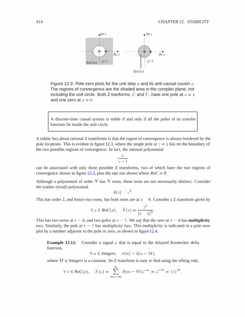
414 CHAPTER 12. STABILITY
|z|=1
Re z
Im z
RoC(u) |z|=1
Re z
Im z
RoC(v)
Figure 12.3: Pole-zero plots for the unit step 0 and its anti-causal cousin ".The regions of convergence are the shaded area in the complex plane, notincluding the unit circle. Both Z tranforms, �B and �E , have one pole at � � and one zero at � � .
A discrete-time causal system is stable if and only if all the poles of its transferfunction lie inside the unit circle.
A subtle fact about rational Z transforms is that the region of convergence is always bordered by thepole locations. This is evident in figure 12.3, where the single pole at � � lies on the boundary ofthe two possible regions of convergence. In fact, the rational polynomial
�
� �
can be associated with only three possible Z transforms, two of which have the two regions ofconvergence shown in figure 12.3, plus the one not shown where RoC� �.Although a polynomial of order � has � roots, these roots are not necessarily distinct. Considerthe (rather trivial) polynomial
���� � ���
This has order 2, and hence two roots, but both roots are at � � . Consider a Z transform given by
� � RoC���� ����� ���
�� � ���
This has two zeros at � � , and two poles at � � . We say that the zero at � � has multiplicitytwo. Similarly, the pole at � � has multiplicity two. This multiplicity is indicated in a pole-zeroplot by a number adjacent to the pole or zero, as shown in figure12.4.
Example 12.12: Consider a signal � that is equal to the delayed Kronecker deltafunction,
� � Integers� ���� � ���3��
where 3 Integersis a constant. Its Z transform is easy to find using the sifting rule,
� � RoC���� ����� ���
����
�'�3���� � ��� � ��� �

12.2. THE Z TRANSFORM 415
|z|=1
Re z
Im z
RoC(x)
22
Figure 12.4: Poles and zeros with multiplicity greater than one are indicatedby a number next to the cross or circle.
If 3 2 , then this converges absolutely for any � �� . Thus, if 3 2 ,
RoC��� � �� Complex� � �� �
This Z transform has 3 poles at � � . Notice that this region of convergence, appro-priately, has the form of that of a causal signal, figure12.2(a), but where the circle hasradius zero.
If 3 ) , then the region of convergence is the entire set Complex, and the Z transformhas 3 zeros at � � . This signal is anti-causal, and its RoCmatches the structure of12.2(c), where the radius of the circle is infinite. Note that this Z transform does notconverge at infinity, which it would have to do if the signal were causal.
If 3 � , then ����� � for all � Complex, so RoC� Complex, and there are nopoles or zeros. This is a particularly simple Z transform.
Recall that for a causal signal, the Z transform must converge as � ��. The region of convergencemust include everything outside some circle, including infinity.1 This implies that for a causal signalwith a rational Z transform, the Z transform must be proper. A rational polynomial is proper whenthe order of the numerator is smaller than or equal to the order of the denominator. For example, if3 � � in the previous example, then ���� � ���� and �;��� � �, which has numerator orderone and denominator order zero. It is not proper, and indeed, it does not converge as � ��. Anyrational polynomial that has a denominator of higher order than the numerator will not converge as� goes to infinity, and hence cannot be the Z transform of a causal signal.
In the following chapter, table 13.1 gives many common Z tranforms, all of which are rationalpolynomials. Together with the properties discussed in the that chapter, we can find the Z transformsof many signals.
1Some texts consider poles and zeros at infinity, in which case a causal signal cannot have a pole at infinity.
416 CHAPTER 12. STABILITY
12.3 The Laplace transform
Consider a continuous-time signal � that is not absolutely integrable. Consider the scaled signal �4given by2
� Reals� �4�� � �����4�� (12.14)
for some real number @. Often, this signal is absolutely integrable when @ is chosen appropriately.This new signal, therefore, will have a CTFT, even if � does not.
Example 12.13: Consider the impulse response of the simplified helicopter systemdescribed in example 12.2. The output as a function of the input is given by
� Reals� ��� �
3
���
�������
The impulse response is found by letting the input be a Dirac delta function and usingthe sifting rule to get
� Reals� ��� � 0���3�
where 0 is the continuous-time unit step in (12.4). This is not absolutely integrable, sothis system is not stable. However, the scaled signal
� Reals� �4�� � �����4�
is absolutely integrable if @ 2 . Its CTFT is
� @ 2 ��� Reals� ;4��� �
����
�����4�������
�
3
���
��4�������
�
3
���
�� 4������
�
3�@ � &���
The last step in example 12.13 uses the following useful fact from calculus,
���
���� �
!���� � ���� � (12.15)
2The reason that this is different from the scaling by -� used to get the Z transform is somewhat subtle. The twomethods are essentially equivalent, if we let - � ��. But scaling by �� turns out to be more convenient for continuous-time systems, as we will see.

12.3. THE LAPLACE TRANSFORM 417
for any ! Complexand �� � Reals� ����� where ��� and ��� are finite.
In general, the CTFT of the scaled signal �4 in (12.14) is
� � Reals� �4��� �
� �
������� 4�������
Notice that this is a function not just of �, but also of @. We are only sure it is valid for values of @that yield an absolutely integrable signal �4 .
Define the complex number� � @ � &��
Then we can write this CTFT as
� � RoC���� ����� ��"
����������� (12.16)
where �� is a function called the Laplace transform of �,
���RoC���� Complex
where RoC��� � Complexis given by
RoC��� � �� � @ � &� Complex� �����4� is absolutely integrable. (12.17)
The Laplace tranform �; of the impulse response � of an LTI system is called the transfer functionof the system, just as with discrete-time systems.
Example 12.14: Continuing example 12.13, we can recognize from the form of ;4���that the transfer function of the helicopter system is
� � RoC���� �;��� �
3��
The RoCisRoC��� � �� � @ � &� Complex� @ )
12.3.1 Structure of the region of convergence
As with the Z transform, the region of convergence is an essential part of a Laplace transform. Itgives the domain of the function �� . Whether a complex number � is in the RoCdepends only on@, not on �, as is evident in the definition (12.17). Since � � @ � &�, whether a complex number isin the region of convergence depends only on its real part. Once again, there are only three possiblepatterns for the region of convergence, shown in figure 12.5. Each figure illustrates the complexplane, and the shaded area is a region of convergence. Each possibility has vertical symmetry, inthat whether a point is in the RoCdepends only on its real part.

418 CHAPTER 12. STABILITY
Re s
Im sIm s
Re s
Im s
causal or right-sided
Re s
anti-causal or left-sidedtwo-sided
RoC RoC RoC
(a) (b) (c)
Figure 12.5: Three possible structures for the region of convergence of aLaplace transform.
Figure 12.5(a) shows the RoCof a causal or right-sided signal. A continuous-time signal � is right-sided if ��� � for all ) for some Reals. The RoC is the set of complex numbers� � @ � &� where following integral converges:
����
������4����
But if � is right-sided, then
����
������4��� ����
������4����
If � and this integral converges for some given @, then it must also converge for any "@ 2 @because for all � , ���4� ) ��4�. Thus, if � � @ � &� RoC���, then the RoC��� must includeall points in the complex plane on the vertical line passing through � and every point to the right ofthat line.3
If ) , then���
������4��� ���
�
������4�������
������4����
then the finite integral exists and is finite for all @, so the same argument applies.
Figure 12.5(c) shows the RoC of a left-sided signal. A continuous-time signal � is left-sided if��� � for all 2 for some Reals. By a similar argument, if � � @ � &� RoC���, thenthe RoC��� must include all points in the complex plane on the vertical line passing through � andevery point to the left of that line.
Figure 12.5(b) shows the RoCof a signal that is a two-sided signal. Such a signal can always beexpressed as a sum of a right-sided signal and left-sided signal. The RoCis the intersection of theregions of convergence for these two components.
3It is convenient but coincidental that the region of convergence is the right half of a plane when the sequence is rightsided.
12.3. THE LAPLACE TRANSFORM 419
Example 12.15: Using the same methods as in examples 12.13 and 12.14 we can findthe Laplace transform of the continuous-time unit step signal 0, given by
� Reals� 0�� �
�� ) � �
� (12.18)
The Laplace transform is
� � RoC�0�� �B��� �
����
0�������
�
���
�����
�
��
where again we have used (12.15). The domain of �B is
RoC�0� � �� Complex� Re�� 2 �This region of convergence has the structure of figure 12.5(a), where the dashed linesits exactly on the imaginary axis. The region of convergence, therefore, is simply theright half of the complex plane.
Example 12.16: The signal " given by
� Reals� "�� � �0��� ���� ) � �
�
has Laplace transform
� � RoC�"�� �E ��� �
����
"�������
� ���
��
�����
�
�
with domainRoC�"� � �� Complex� Re�� ) �
This region of convergence has the structure of figure 12.5(c), where the dashed linecoincides with the imaginary axis.
Notice that although the Laplace transforms �B and �E have the same algebraic form, namely, ��,they are in fact different functions, because their domains are different.
Some signals have no meaningful Laplace transform.
420 CHAPTER 12. STABILITY
Example 12.17: The signal � with ��� � , for all Reals, does not have aLaplace transform. We can write � � 0� ", where 0 and " are defined in the previousexamples. Thus, the region of convergence of � must be the intersection of the regionsof convergence of 0 and ". However, these two regions have an empty intersection, soRoC��� � �.Viewed another way, the set RoC��� is the set of complex numbers � where
����
���������� ���
��
������� )��
But there is no such complex number �.
Note that the signal � in example 12.17 is periodic with any period ( Reals(because ��� (� ���� for any ( Reals). Thus, it has a Fourier series representation. In fact, as shown in section10.6.3, a periodic signal also has a Fourier transform representation, as long as we are willing toallow Dirac delta functions in the Fourier transform. (Recall that this means that there are valuesof � where ���� will not be finite.) In the continuous-time case as in the discrete-time case, withperiodic signals, the Fourier series is by far the simplest frequency-domain tool to use. The Fouriertransform can also be used if we allow Dirac delta functions. The Laplace transform, however, ismore problematic, because the region of convergence is empty.
12.3.2 Stability and the Laplace transform
If a continuous-time signal � is absolutely integrable, then it has a CTFT � that is finite for all� Reals. Moreover, the CTFT is equal to the Laplace transform evaluated on the imaginary axis,
� � Reals� ���� � ���������� � ���&���
The complex number � � &� is pure imaginary, and therefore lies on the imaginary axis. Recall thatan LTI system is stable if and only if its impulse response is absolutely integrable. Thus
A continuous-time LTI system with impulse response � is stable if an only if thetransfer function �; , which is the Laplace transform of �, has a region of conver-gence that includes the imaginary axis.
Example 12.18: Consider the exponential signal � given by
� Reals� ��� � ����0���
for some real or complex number �, where, as usual, 0 is the unit step. The Laplacetransform is
� � RoC���� �;��� �
����
��������
12.3. THE LAPLACE TRANSFORM 421
�
���
���������
�
���
�� ������
�
�� ��
where again we have used (12.15). It is evident from (12.15) that for this integral to bevalid, the domain of �; must be
RoC��� � �� Complex� Re�� 2 �Re���This region of convergence has the structure of figure12.5(a), where the vertical dashedline passes through �.
Now suppose that � is the impulse response of an LTI system. That LTI system isstable if an only if Re�� 2 . Indeed, if Re�� ) , then the impulse response growswithout bound, because ���� grows without bound as gets large.
12.3.3 Rational Laplace tranforms and poles and zeros
All of the Laplace transforms we have seen so far are rational polynomials in �. In practice, mostLaplace transforms of interest can be written as the ratio of two finite order polynomials in �,
����� �����
�����
An exception is illustrated in the following example.
Example 12.19: Consider a signal � that is equal to the delayed Dirac delta function,
� Reals� ��� � �� ���
where � Realsis a constant. Its Laplace transform is easy to find using the siftingrule,
� � RoC���� ����� �
����
� � ������� � ���( �
This has no finite-order rational polynomial representation.
Unlike the discrete-time case, pure time delays turn out to be rather difficult to realize in manyphysical systems that are studied using Laplace transforms, so we need not be overly concernedwith them. We focus henceforth on rational Laplace transforms.
For a rational Laplace transform, the order of the polynomial � or � is the power of the highestpower of �. For the exponential of example 12.18, the numerator polynomial is ���� � , a zero-order polynomial, and the denominator is ���� � � � �, a first-order polynomial. As with the Z
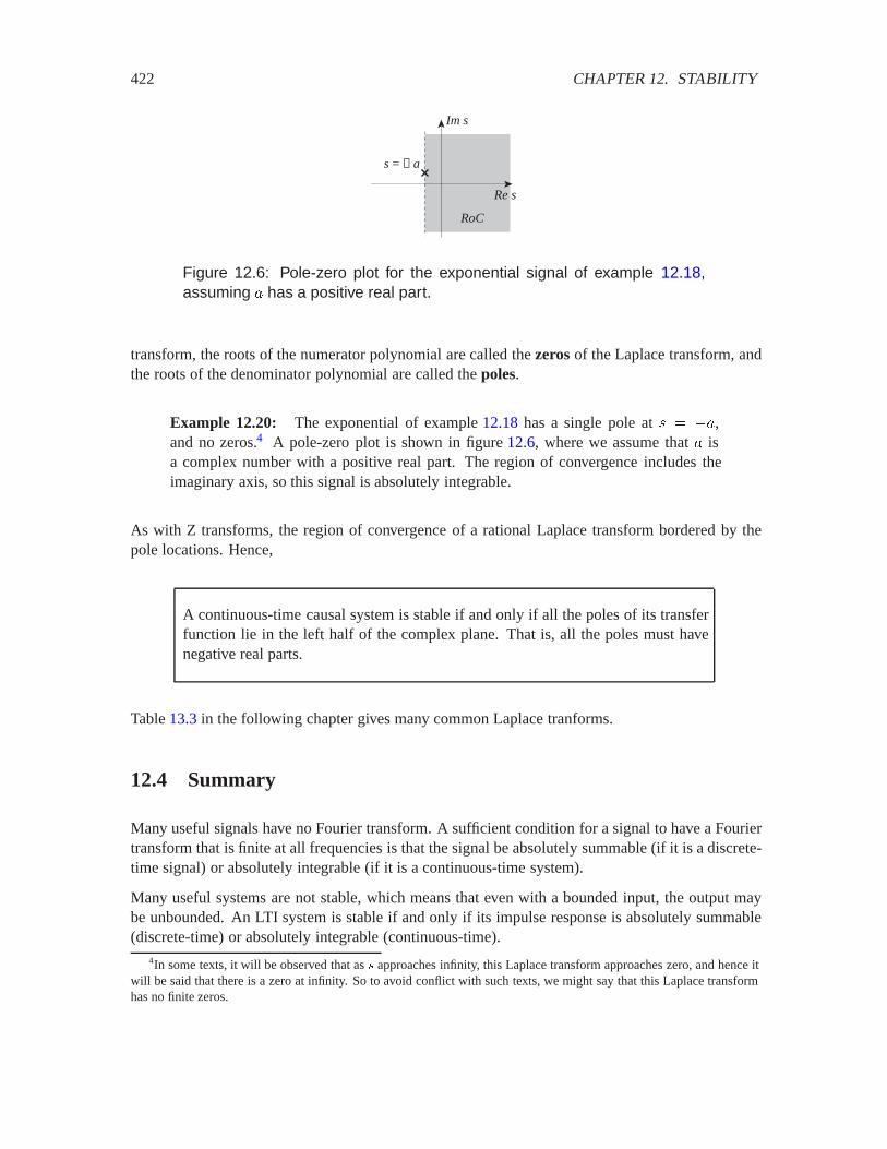
422 CHAPTER 12. STABILITY
Im s
Re s
RoC
s = − a
Figure 12.6: Pole-zero plot for the exponential signal of example 12.18,assuming � has a positive real part.
transform, the roots of the numerator polynomial are called the zeros of the Laplace transform, andthe roots of the denominator polynomial are called the poles.
Example 12.20: The exponential of example 12.18 has a single pole at � � ��,and no zeros.4 A pole-zero plot is shown in figure 12.6, where we assume that � isa complex number with a positive real part. The region of convergence includes theimaginary axis, so this signal is absolutely integrable.
As with Z transforms, the region of convergence of a rational Laplace transform bordered by thepole locations. Hence,
A continuous-time causal system is stable if and only if all the poles of its transferfunction lie in the left half of the complex plane. That is, all the poles must havenegative real parts.
Table 13.3 in the following chapter gives many common Laplace tranforms.
12.4 Summary
Many useful signals have no Fourier transform. A sufficient condition for a signal to have a Fouriertransform that is finite at all frequencies is that the signal be absolutely summable (if it is a discrete-time signal) or absolutely integrable (if it is a continuous-time system).
Many useful systems are not stable, which means that even with a bounded input, the output maybe unbounded. An LTI system is stable if and only if its impulse response is absolutely summable(discrete-time) or absolutely integrable (continuous-time).
4In some texts, it will be observed that as . approaches infinity, this Laplace transform approaches zero, and hence itwill be said that there is a zero at infinity. So to avoid conflict with such texts, we might say that this Laplace transformhas no finite zeros.
12.4. SUMMARY 423
Many signals that are not absolutely summable (integrable) can be scaled by an exponential to geta new signal that is absolutely summable (integrable). The DTFT (CTFT) of the scaled signal iscalled the Z transform (Laplace transform) of the signal.
The Z transform (Laplace transform) is defined over a region of convergence, where the structureof the region of convergence depends on whether the signal is causal, anti-causal, or two-sided.The Z transform (Laplace transform) of the impulse response is called the transfer function of anLTI system. The region of convergence includes the unit circle (imaginary axis), if and only if thesystem is stable.
A rational Z transform (Laplace transform) has poles and zeros, and the poles bound the region ofconvergence. The locations of the poles and zeros yield considerable information about the system,including whether it is stable.
Exercises
Each problem is annotated with the letter E, T, C which stands for exercise, requires some thought,requires some conceptualization. Problems labeled E are usually mechanical, those labeled T re-quire a plan of attack, those labeled C usually have more than one defensible answer.
1. E Consider the signal � given by
� � Integers� ���� � ��0�����
where � is a complex constant.
(a) Find the Z transform of �. Be sure to give the region of convergence.
(b) Where are the poles and zeros?
(c) Under what conditions on � is � absolutely summable?
(d) Assuming that � is absolutely summable, find its DTFT.
2. T Consider the signal � given by
� � Integers� ���� �
�� ��� �3� otherwise
�
for some integer 3 2 .
(a) Find the Z transform of �. Simplify so that there remain no summations. Be sure to givethe region of convergence.
(b) Where are the poles and zeros? Do not give poles and zeros that cancel each other out.
(c) Under what conditions is � absolutely summable?
(d) Assuming that � is absolutely summable, find its DTFT.
424 CHAPTER 12. STABILITY
3. T Consider the unit ramp signal / given by
� � Integers� /��� � �0����
where 0 is the unit step. The following identity will be useful,
�����
�'� ��� � ���
���
���� �
�� ���� (12.19)
This is a generalization of the geometric series identity, given by (12.9). This series convergesfor any complex number � with ��� ) , because
�����
�'� ����� � � ����� ����� �
� � � ���� ���� � �� � ���� ���� � �
� ���
���
������
) ��
(a) Use the given identity to find the Z transform of the unit ramp. Be sure to give the regionof convergence. Check your answer against that given on page438.
(b) Sketch the pole-zero plot of the Z transform.
(c) Is the unit ramp absolutely summable?
4. E Sketch the pole-zero plots and regions of convergence for the Z transforms of the follow-ing impulse responses, and indicate whether a discrete-time LTI system with these impulseresponses is stable:
(a) ����� � ��� � ���� � �.
(b) ����� � �����0���.
(c) ����� � ��0���.
5. E Consider the anti-causal continuous-time exponential signal � given by
� Reals� ��� � �����0����
for some real or complex number �, where, as usual, 0 is the unit step.
(a) Show that the Laplace transform of � is
����� �
�� �
with region of convergence
RoC��� � �� Complex� Re�� ) �Re���
(b) Where are the poles and zeros?
12.4. SUMMARY 425
(c) Under what conditions on � is � absolutely integrable?
(d) Assuming that � is absolutely integrable, find its CTFT.
6. E This exercise demonstrates that the Laplace transform is linear. Show that if � and � arecontinuous-time signals, � and � are complex (or real) constants, and / is given by
� Reals� /�� � ���� � �����
then the Laplace transform is
� � RoC�/�� �7 ��� � � ����� � � �$ ����
whereRoC�/� RoC��� � RoC����
7. T Let the causal sinusoidal signal � be given by
� Reals� ��� � �������0���
where �� is a real number and 0 is the unit step.
(a) Show that the Laplace transform is
� � �� � Re�� 2 � �$ ��� ��
�� � ����
Hint: Use linearity, demonstrated in exercise 6, and Euler’s relation.
(b) Sketch the pole-zero plot and show the region of convergence.
8. E Consider a discrete-time LTI system with impulse response
��� ���� � �� ��������0����
for some �� Reals. Determine for what values of � this system is stable.
9. T The continuous-time unit ramp signal / is given by
� Reals� ��� � 0���
where 0 is the unit step.
(a) Find the Laplace transform of the unit ramp, and give the region of convergence.Hint: Use integration by parts in (12.16) and the fact that
"�� ��4�� )� for @ 2 .
(b) Sketch the pole-zero plot of the Laplace transform.
10. E Let � and � be the impulse response of two stable systems. They may be discrete-time orcontinuous-time. Let � and � be two complex numbers. Show that the system with impulseresponse ��� �� is stable.

426 CHAPTER 12. STABILITY
x y
h1
h2 g2
g1
+
Figure 12.7: System composition for exercise 13.
11. T Consider a series composition of two (continuous- or discrete-time) systems with impulseresponse � and �. The output " of the first system is related to its input � by " � � � �. Theoutput � of the second system (and of the series composition) is � � � � ". Suppose bothsystems are stable. Show that the series composition is stable.Hint: Use the definition of stability.
12. T Let � be the impulse response of a stable discrete-time system, so it is absolutely summable,and denote
!�! ���
����
�������
(!�! is called the norm of the impulse response.)
(a) Suppose the input signal � is bounded by 3 , i.e. ��� ������ �3 . Show that the output� � � � � is bounded by !�!3 .
(b) Consider the input signal � where
�� Integers� ���� �
��������������� ���� �� � ���� � �
Show that !�! is the smallest bound of the output � � � � �.
(c) Let � be the impulse response of another stable system with norm !�!. Show that thenorm satisfies the triangle inequality,
!�� �! � !�! � !�!�
(d) Suppose the two systems are placed in series. The composition has the impulse response� � �. Show that
!� � �! � !�! � !�!�13. E Show that the series-parallel composition of figure 12.7 is stable if the four component
systems are stable. Let � be the impulse response of the composition. Express � in termsof the component impulse responses and then estimate !�! in terms of the norms of thecomponents.
14. E Let � be a discrete-time signal of finite duration, i.e. ���� � for � ) 3 and � 2 �where 3 and � are finite integers (positive or negative). Let �� be its Z transform.
(a) Show that all its poles (if any) are at � � .
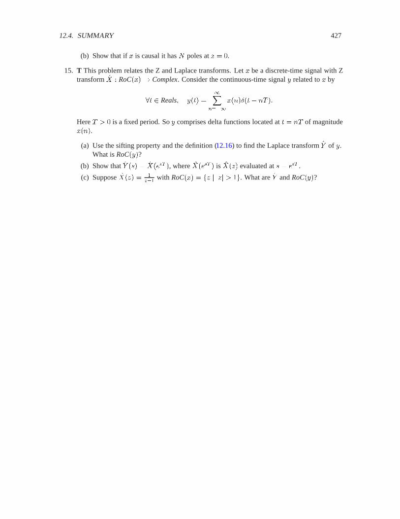
12.4. SUMMARY 427
(b) Show that if � is causal it has � poles at � � .
15. T This problem relates the Z and Laplace transforms. Let � be a discrete-time signal with Ztransform �� � RoC���� Complex. Consider the continuous-time signal � related to � by
� Reals� ��� ���
����
����� � � ��
Here 2 is a fixed period. So � comprises delta functions located at � � of magnitude����.
(a) Use the sifting property and the definition (12.16) to find the Laplace transform �$ of �.What is RoC���?
(b) Show that �$ ��� � ������ �, where ������ � is ����� evaluated at � � ��� .
(c) Suppose ����� � ���� with RoC��� � �� � ��� 2 . What are �$ and RoC���?

428 CHAPTER 12. STABILITY

Chapter 13
Laplace and Z Transforms
In the previous chapter, we defined Laplace and Z transforms to deal with signals that are notabsolutely summable and systems that are not stable. The Z transform of the discrete-time signal �is given by
� � RoC���� ����� ���
����
��'�����
where RoC��� is the region of convergence, the region in which the sum above converges abso-lutely.
The Laplace transform of the continuous-time signal � is given by
� � RoC���� ����� �
����
���������
where RoC��� is again the region of convergence, the region in which the integral above convergesabsolutely.
In this chapter, we explore key properties of the Z and Laplace transforms and give examples oftransforms. We will also explain how, given a rational polynomial in � or �, plus a region ofconvergence, one can find the corresponding time-domain function. This inverse transform provesparticularly useful, because compositions of LTI systems, studied in the next chapter, often lead torather complicated rational polynomial descriptions of a transfer function.
Z transforms of common signals are given in table 13.1. Properties of the Z transform are summa-rized in table 13.2 and elaborated in the first section below.
13.1 Properties of the Z tranform
The Z transform has useful properties that are similar to those of the four Fourier transforms. Theyare summarized in table 13.2 and elaborated in this section.
429
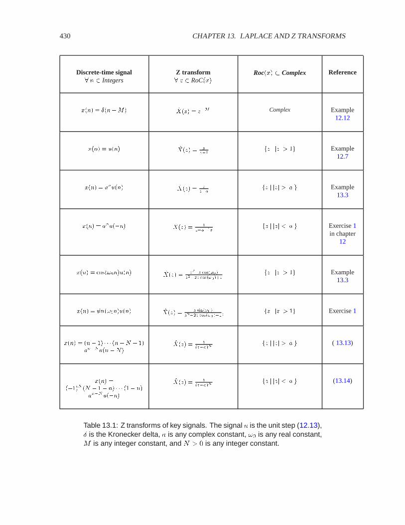
430 CHAPTER 13. LAPLACE AND Z TRANSFORMS
Discrete-time signal� � � Integers
Z transform� � � RoC���
Roc��� � Complex Reference
���� � ����� ���/� � /� Complex Example12.12
���� � "��� ���/� � ���
/ / � �� Example12.7
���� � ��"��� ���/� � ���
/ / � �� Example13.3
���� � ��"���� ���/� � ������
/ / � �� Exercise 1in chapter
12
���� � �������"��� ���/� � ��� �����
���� �������/ / � �� Example
13.3
���� � �������"��� ���/� � � � ���
���� �������� / / � �� Exercise 1
���� � ��� �� � � � ���� � �����"�� ���
���/� � �����
/ / � �� ( 13.13)
���� ������ �� � �� �� � � � ��� ��
���"����
���/� � �����
/ / � �� (13.14)
Table 13.1: Z transforms of key signals. The signal 0 is the unit step (12.13),Æ is the Kronecker delta, � is any complex constant, �� is any real constant,3 is any integer constant, and � 2 is any integer constant.
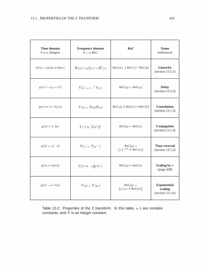
13.1. PROPERTIES OF THE Z TRANFORM 431
Time domain� � � Integers
Frequency domain� � � RoC
RoC Name(reference)
)��� � ����� � (&��� �# �/� � � ���/� � ( �' �/� RoC�)� � RoC����RoC�&� Linearity(section 13.1.1)
&��� � ������ �' �/� � /� ���/� RoC�&� � RoC��� Delay(section 13.1.2)
&��� � �� � *���� �' �/� � ���/� �+�/� RoC�&� � RoC��� � RoC�*� Convolution(section 13.1.3)
&��� � ����� �' �/� � � ���/���� RoC�&� � RoC��� Conjugation(section 13.1.4)
&��� � ����� �' �/� � ���/�� RoC�&� �/ /� � RoC����
Time reversal(section 13.1.5)
&��� � ����� �' �/� � �/ ���
���/� RoC�&� � RoC��� Scaling by �
(page 438)
&��� � ������ �' �/� � ����/� RoC�&� �/ �/ � RoC����
Exponentialscaling
(section 13.1.6)
Table 13.2: Properties of the Z transform. In this table, �� � are complexconstants, and � is an integer constant.

432 CHAPTER 13. LAPLACE AND Z TRANSFORMS
13.1.1 Linearity
Suppose � and � have Z transforms �� and �$ , that �� � are two complex constants, and that
/ � ��� ���
Then the Z transform of / is
� � RoC�/�� �7 ��� � � ����� � � �$ ����
This follows immediately from the definition of the Z transform,
�7 ��� ���
����
/�'����
���
����
����'� � ���'�����
� � ����� � � �$ ����
The region of convergence of / must include at least the regions of convergence of � and �, sinceif ������� and ������� are absolutely summable, then certainly ������� ��������� is absolutelysummable. Conceivably, however, the region of convergence may be larger. Thus, all we can assertin general is
RoC�/� RoC��� �RoC���� (13.1)
Linearity is extremely useful because it makes it easy to find the Z transform of complicated signalsthat can be expressed a linear combination of signals with known Z transforms.
Example 13.1: We can use the results of example 12.12 plus linearity to find, forexample, the Z transform of the signal � given by
� � Integers� ���� � ��� � ���� � �� � ���� � ���
This is simply����� � � ���� � ������
We can identify the poles by writing this as a rational polynomial in � (multiply top andbottom by ��),
����� ��� � ��� � ��
���
from which we see that there are 5 poles at � � . The signal is causal, so the regionof convergence is the region outside the circle passing through the pole with the largestmagnitude, or in this case,
RoC��� � �� Complex� � �� �
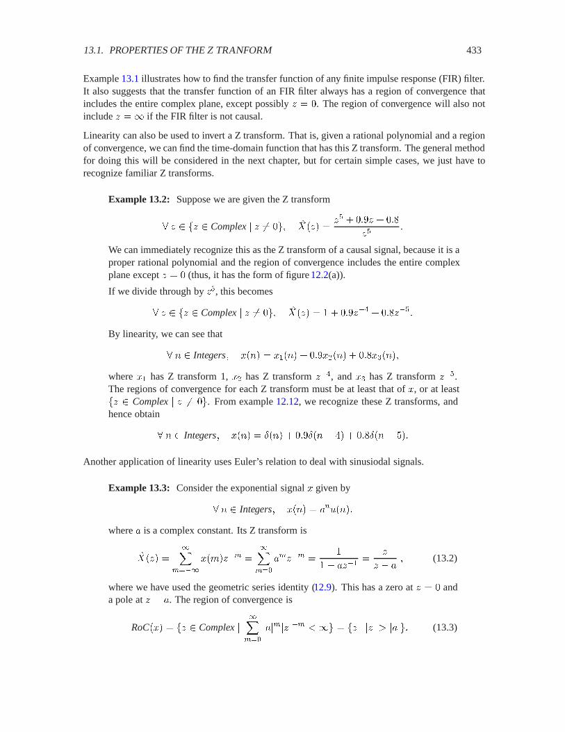
13.1. PROPERTIES OF THE Z TRANFORM 433
Example 13.1 illustrates how to find the transfer function of any finite impulse response (FIR) filter.It also suggests that the transfer function of an FIR filter always has a region of convergence thatincludes the entire complex plane, except possibly � � . The region of convergence will also notinclude � �� if the FIR filter is not causal.
Linearity can also be used to invert a Z transform. That is, given a rational polynomial and a regionof convergence, we can find the time-domain function that has this Z transform. The general methodfor doing this will be considered in the next chapter, but for certain simple cases, we just have torecognize familiar Z transforms.
Example 13.2: Suppose we are given the Z transform
� � �� Complex� � �� � ����� ��� � ��� � ��
���
We can immediately recognize this as the Z transform of a causal signal, because it is aproper rational polynomial and the region of convergence includes the entire complexplane except � � (thus, it has the form of figure 12.2(a)).
If we divide through by ��, this becomes
� � �� Complex� � �� � ����� � � ���� � ������
By linearity, we can see that
� � Integers� ���� � ����� � ������� � ��������
where �� has Z transform 1, �� has Z transform ��, and �� has Z transform ���.The regions of convergence for each Z transform must be at least that of �, or at least�� Complex� � �� . From example 12.12, we recognize these Z transforms, andhence obtain
� � Integers� ���� � ��� � ���� � �� � ���� � ���
Another application of linearity uses Euler’s relation to deal with sinusiodal signals.
Example 13.3: Consider the exponential signal � given by
� � Integers� ���� � ��0����
where � is a complex constant. Its Z transform is
����� ���
����
��'���� ���
���
����� �
� �����
�
� � �� (13.2)
where we have used the geometric series identity (12.9). This has a zero at � � anda pole at � � �. The region of convergence is
RoC��� � �� Complex���
���
��������� )� � �� � ��� 2 ���� (13.3)
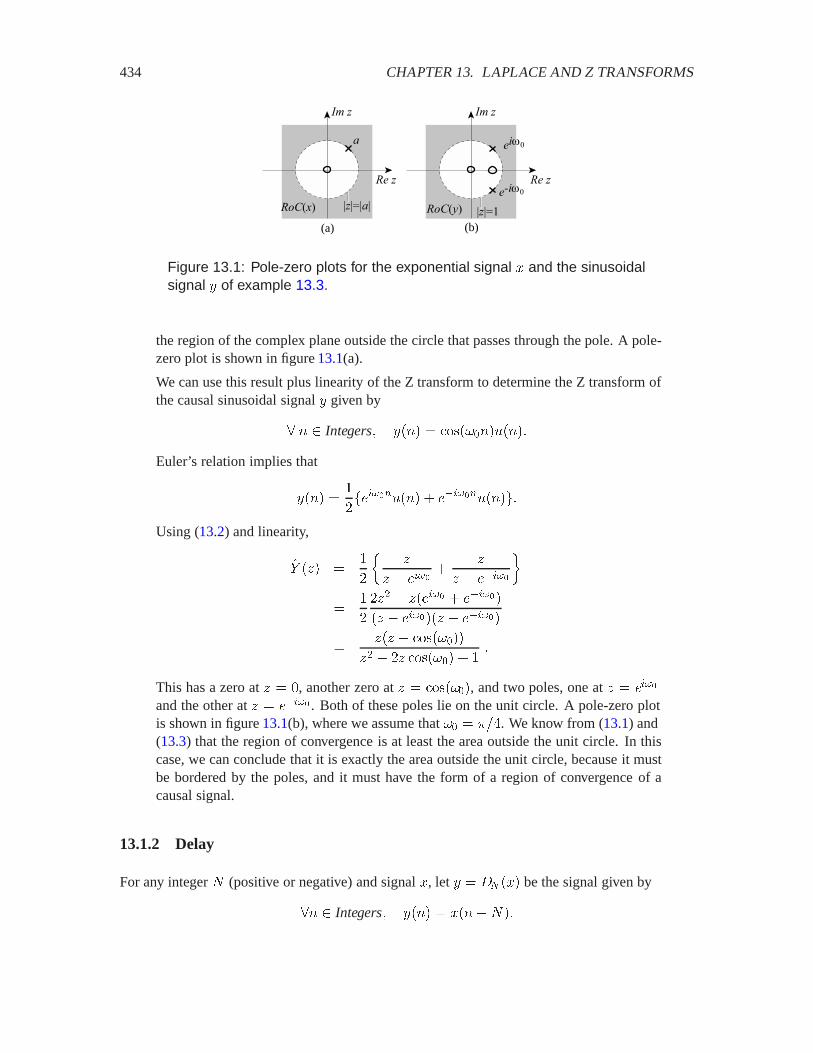
434 CHAPTER 13. LAPLACE AND Z TRANSFORMS
Re z
Im z
RoC(x) |z|=1
Re z
Im z
RoC(y)
a
|z|=|a|
eiω0
e-iω0
(a) (b)
Figure 13.1: Pole-zero plots for the exponential signal � and the sinusoidalsignal � of example 13.3.
the region of the complex plane outside the circle that passes through the pole. A pole-zero plot is shown in figure 13.1(a).
We can use this result plus linearity of the Z transform to determine the Z transform ofthe causal sinusoidal signal � given by
� � Integers� ���� � ��������0����
Euler’s relation implies that
���� �
�������0��� � ������0����
Using (13.2) and linearity,
�$ ��� �
�
��
� � �����
�
� � �����
�
�
��� � ������ � ������
�� � ������� � ������
���� � ��������
�� � �� ������� � �
This has a zero at � � , another zero at � � �������, and two poles, one at � � ����
and the other at � � ����� . Both of these poles lie on the unit circle. A pole-zero plotis shown in figure 13.1(b), where we assume that �� � ���. We know from (13.1) and(13.3) that the region of convergence is at least the area outside the unit circle. In thiscase, we can conclude that it is exactly the area outside the unit circle, because it mustbe bordered by the poles, and it must have the form of a region of convergence of acausal signal.
13.1.2 Delay
For any integer � (positive or negative) and signal �, let � � �� ��� be the signal given by
�� Integers� ���� � �������
13.1. PROPERTIES OF THE Z TRANFORM 435
Suppose � has Z transform �� with domain RoC���. Then RoC��� � RoC��� and
�� RoC���� �$ ��� ���
����
��'���� ���
����
��'������ � ��� ������ (13.4)
Thus
If a signal is delayed by � samples, its Z transform is multiplied by ��� .
13.1.3 Convolution
Suppose � and � have Z transforms �� and �; . Let
� � � � ��Then
�� RoC���� �$ ��� � ����� �;���� (13.5)
This follows from using the definition of convolution,
�� Integers� ���� ���
����
��'�����'��
in the definition of the Z transform,
�$ ��� ���
����
������� ���
����
������
��'��������'��� ����
���
���
������
��'������,��� � ����� �;����
The Z transform of � converges absolutely at least at values of � where both �� and �; convergeabsolutely. Thus,
RoC��� RoC��� �RoC����
This is true because the double sum above can be written as
������
������� �
���
����
��'����
�$% �� ���
��,���
&' �
This obviously converges absolutely if each of the two factors converges absolutely. Note that theregion of convergence may actually be larger than RoC��� � RoC���. This can occur, for example,if the product (13.5) results in zeros of ����� cancelling poles of �;��� (see exercise 3).
If � is the impulse response of an LTI system, then its Z transform is called the transfer functionof the system. The result (13.5) tells us that the Z transform of the output is the product of the Ztransform of the input and the transfer function. The transfer function, therefore, serves the samerole as the frequency response. It converts convolution into simple multiplication.

436 CHAPTER 13. LAPLACE AND Z TRANSFORMS
13.1.4 Conjugation
Suppose � is a complex-valued signal. Let � be defined by
� � Integers� ���� � ��������
Then� � RoC���� �$ ��� � � ���������
whereRoC��� � RoC����
This follows because
� � RoC���� �$ ��� ���
����
�������
���
����
��������
�
��
����
����������
��
� � ���������
If � happens to be a real signal, then � � �, so �$ � �� , so
����� � � ���������
The key consequence is:
For the Z transform of a real-valued signal, poles and zeros occur in complex-conjugate pairs. That is, if there is a zero at � � 8, then there must be a zero at� � 8�, and if there is a pole at � � (, then there must be a pole at � � (�.
This is because � ���8� � � ���8����
Similarly, if there is a pole at � � (, then there must also be a pole at � � (�.
Example 13.4: Example 13.3 gave the Z transform of a signal of the form ���� ���0���, where � is allowed to be complex, and the Z tranform of a signal of the form���� � ��������0���, which is real-valued. The pole-zero plots are shown in figure13.1. In that figure, the complex signal has a pole at � � �, and none at � � ��. Butthe real signal has a pole at � � ���� and a matching pole at the complex conjugate,� � ����� .
13.1. PROPERTIES OF THE Z TRANFORM 437
13.1.5 Time reversal
Suppose � has Z transform �� and � is obtained from � by reversing time, so that
� � Integers� ���� � ������
Then�� �� Complex� ��� Roc���� �$ ��� � ��������
This is evident from the definition of the Z transform, which implies that
�$ ��� ���
����
���'���� ���
����
����������� � ��������
where ������� is �� evaluated at ���.
13.1.6 Multiplication by an exponential
Suppose � has Z transform �� , � is a complex constant, and ���� � ������� for all �. Then
�� �� Complex� �� RoC���� �$ ��� � �������
where ������ is �� evaluated at ��. This is because
�$ ��� ���
����
��'���� ���
����
��'������� � �������
Note that if �� has a pole at ( (or a zero at 8), then �$ has a pole at (�� (or a zero at 8��).
Example 13.5: Suppose � is given by
� � Integers� ���� � ��0����
Then we know from example 13.3 that
� � �� � ��� 2 ���� ����� ��
� � ��
This has a pole at � � �. Now let ���� � ������� � 0���. The Z transform is
�$ ��� � ������ ���
�� � ��
�
� � �
as expected. Moreover, this has a pole at � � ��� � , as expected, and the region ofconvergence is indeed given by
�� Complex� �� RoC��� � �� Complex� ��� 2 �

438 CHAPTER 13. LAPLACE AND Z TRANSFORMS
Probing further: Derivatives of Z transforms
Calculus on complex-valued functions of complex variables can be somewhat intri-cate. Suppose �� is a function of a complex variable. The derivative can be definedas a limit,
�
������� � !��
0�
���� � A�� �����
A�
where A is a complex variable that can approach zero from any direction in thecomplex plane. The derivative exists if the limit does not depend on the direction.If the derivative exists at all points within a distance A 2 of a point � in thecomplex plane, then �� is said to be analytic at �. A Z transform is a series of theform
� � RoC���� ����� ���
����
��������
This is called a Laurent series in the theory of complex variables. It can be shownthat a Laurent series is analytic at all points � RoC���, and that the derivative is
� � RoC�����
������� �
������
�'��'�������
We can use this fact to show that the Z transform of � given by ���� � ����� is
�� Roc���� �$ ��� � �� ���
������
This is because
�$ ��� ���
����
�������� ���
����
���� ���������� � �� �
��������
It is not difficult to show that Roc��� � Roc��� (see exercise 5).
This property can be used to find other Z transforms. For example, the Z transformof the unit step, � � 0, is ����� � ������, with RoC��� � �� Complex� ��� 2. So the Z transform of the unit ramp �, given by ���� � �0���, is
�$ ��� � �� ���
�
� � �
�
�� � ���
with RoC��� � �� Complex� ��� 2 . Another method for finding the Ztransform of the unit ramp is given in exercise 3 of chapter 12.
13.1. PROPERTIES OF THE Z TRANFORM 439
13.1.7 Causal signals and the initial value theorem
Consider a causal discrete-time signal �. Its Z transform is
� � �� Complex� ��� 2 �� ����� ���
���
��'�����
for some � (the largest magnitude of a pole). Then
!����
�����
��'���� � ��� � !����
�����
��'���� � ����
This is because as � goes to�, each term ��'���� goes to zero. Thus
If � is causal, ��� � !����
����� �
This is called the initial value theorem.
Example 13.6: The Z transform of the unit step ���� � 0��� is ����� � ���� � �,so, as expected,
��� � !����
����� � !����
�
� � � !��
��
� ���� �
because!����
��� � �
Suppose a Z transform �� is the rational polynomial
����� ����� � �����
��� � ���� � �������� � � ��
�
If � is causal, then this rational polynomial must be proper. Were this not the case, if 3 2 � , thenby the initial value theorem, we would have
��� � !����
����� ���
which is certainly not right.
Example 13.7: Consider the Z transform
� � Complex� ����� � ��
This is not a proper rational polynomial (the numerator has order 1 and the denominator,which is 1, has order 0). From example 12.12, we know that this corresponds to
� � Integers� ���� � ��� ��
This is not a causal signal.

440 CHAPTER 13. LAPLACE AND Z TRANSFORMS
13.2 Frequency response and pole-zero plots
A pole-zero plot can be used to get a quick estimate of key properties of an LTI system. We havealready seen that it reveals whether the system is stable. It also reveals key features of the frequencyresponse, such as whether the system is highpass or lowpass.
Consider a stable discrete-time LTI system with impulse response �, frequency response ; , andrational transfer function �; . We know that the frequency response and transfer function are relatedby
�� Reals� ;��� � �;������
That is, the frequency response is equal to the Z transform evaluated on the unit circle. The unitcircle is in the region of convergence because the system is stable.
Assume that �; is a rational polynomial, in which case we can express it in terms of the first-orderfactors of the numerator and denominator polynomials,
�;��� ��� � 8�� �� � 8��
�� � (�� �� � (� ��
with zeros at 8�� � 8� and poles at (�� � (� . The zeros and poles may be repeated (i.e., theymay have multiplicity greater than one). The frequency response is therefore
� � Reals� ;��� ����� � 8�� ���� � 8��
���� � (�� ���� � (� ��
The magnitude response is
� � Reals� �;���� � ���� � 8�� ���� � 8� ����� � (�� ���� � (� � �
Each of these factors has the form���� � ��
where � is the location of either a pole or a zero. The factor ���� � �� is just the distance from ��� to� in the complex plane.
Of course, ��� is a point on the unit circle. If that point is close to a zero at location 8, then the factor���� � 8� is small, so the magnitude response will be small. If that point is close to a pole at (, thenthe factor ���� � (� is small, but since this factor is in the denominator, the magnitude response willbe large. Thus,
The magnitude response of a stable LTI system may be estimated from the pole-zero plot of its transfer function. Starting at � � , trace counterclockwise aroundthe unit circle as � increases. If you pass near a zero, then the magnitude responseshould dip. If you pass near a pole, then the magnitude response should rise.

13.2. FREQUENCY RESPONSE AND POLE-ZERO PLOTS 441
Example 13.8: Consider the causal LTI system of example 9.16, which is defined bythe difference equation
� � Integers� ���� � ���� � ������ ��
We can find the transfer function by taking Z transforms on both sides, using linearity,to get
�$ ��� � ����� � ����� �$ ����
The transfer function is
�;��� ��$ ��������
�
� ������
�
� � ���
This has a pole at � � ��, which is closest to � � on the unit circle, and a zero at� � , which is equidistant from all points on the unit circle. The zero, therefore, hasno effect on the magnitude response. The pole is closest to � � , which correspondsto � � , so the magnitude response peaks at � � , as shown in figure9.12.
Example 13.9: Consider a legnth-4 moving average. Using methods like those inexample 9.12, we can show that the transfer function is
� � �� Complex� � �� � �;��� �
� � ��
� ����
�
� �
���� � ��
The numerator polynomial has roots at the four roots of unity, which are � � , � ���)��, � � �, and � � ���)��. Thus, we can write this transfer function as
� � �� Complex� � �� ��;��� �
�
�� � ��� � ��)����� � ��� � ���)���
���� � �
�
�
�� � ��)����� � ��� � ���)���
���
The ��� � factors in the numerator and denominator cancel (fortunately, or we wouldhave a pole at � � , on the unit circle, and we would have to conclude that the systemwas unstable). A pole-zero plot is shown in figure 13.2.
The magnitude response is shown in figure 9.8. Relating that figure to the pole-zeroplot, we see that the frequency response peaks at � � , and as we move around theunit circle, we pass through zero at � � ���, or � � ��)��, and again through zero at� � �. The magnitude response is periodic with period ��, so the zero at � � ���)�� isalso a zero at � � ���)��, corresponding to a frequency of � � ����.

442 CHAPTER 13. LAPLACE AND Z TRANSFORMS
Continuous-time signal� � � Reals
Laplace transform� � � RoC���
Roc(x) Reference
���� � ��� �� ���.� � ��� Complex Exercise12.19
���� � "��� ���.� � ��. . � Complex Re.� � �� Example12.15
���� � ��"������.� �
�
. � �
. � Complex Re.� ��Re���
Example12.18
���� � ���"�������.� �
�
. � �
. � Complex Re.� ��Re���
Exercise 5
���� � �������"������.� �
.
.� � ���
. Re.� � �� Exercise 7
���� � �������"������.� �
��
.� � ���
. Re.� � �� Example13.10
���� ����
�� � �����"��� ���/� �
�
�. � ���
. � Complex Re.� ��Re���
—
���� � � ���
�� � �����"���� ���/� �
�
�. � ���
. � Complex Re.� ��Re���
—
Table 13.3: Laplace transforms of key signals. The signal 0 is the unitstep (12.18), Æ is the Dirac delta, � is any complex constant, �� is any realconstant, � is any real constant, and � is a positive integer.

13.2. FREQUENCY RESPONSE AND POLE-ZERO PLOTS 443
Time domain� � � Reals
� domain� � � RoC
RoC Name(reference)
)��� � ����� � (&��� �# �.� � � ���.� � ( �' �.� RoC�)� � RoC����RoC�&� Linearity(exercise 6)
&��� � ���� �� �' �.� � ��� ���.� RoC�&� � RoC��� Delay(exercise 7)
&��� � �� � *��-� �' �.� � ���.� �+�.� RoC�&� � RoC��� � RoC�*� Convolution(exercise 8)
&��� � ����� �' �.� � � ���.���� RoC�&� � RoC��� Conjugation(exercise 9)
&��� � ��0�� �' �.� � ���.�0��0 RoC�&� �. .�0 � RoC����
Time scaling(exercise 10)
&��� � �����
�' �.� � � %
%.���.�
RoC�&� � RoC��� Scaling by �
—
&��� � ������ �' �.� � ���.� �� RoC�&� �. .� � � RoC����
Exponentialscaling
(exercise 11)
&��� �"
����%��' �.� � ���.��. RoC�&� �
RoC��� � . Re.� � ��Integration
(section 13.3.1)
&��� �%
%�����
�' �.� � . ���.� RoC�&� � RoC��� Differentiation(page 43)
Table 13.4: Properties of the Laplace transform. In this table, �� � are com-plex constants, ! and � are real constants.

444 CHAPTER 13. LAPLACE AND Z TRANSFORMS
|z|=1
Re z
Im z
3
Figure 13.2: Pole-zero plot for a length-4 moving average system.
13.3 Properties of the Laplace transform
The Laplace transform has useful properties that are similar to those of the Z transform. Theyare summarized in table 13.4 and elaborated mostly in the exercises at the end of this chapter. Inthis section, we elaborate on one of the properties that is not shared by the Z transform, namelyintegration, and then use the properties to develop some examples. Key Laplace transforms aregiven in table 13.3.
13.3.1 Integration
Let � be defined by
� Reals� ��� �
����
�������
The Laplace tranform is
� � RoC���� �$ ��� � ��������
where
RoC��� RoC��� � �� � Re�� 2 �
This follows from the convolution property in table13.4. We recognize that
��� � �� � 0����
where 0 is the unit step. Hence, from the convolution property,
�$ ��� � ����� �B���
and
RoC��� RoC��� � RoC�0��
�B and RoC�0� are given in example 12.15, from which the property follows.

13.3. PROPERTIES OF THE LAPLACE TRANSFORM 445
Im s
Re s
RoC
s = iω
s = − iω
Figure 13.3: Pole-zero plot for the sinusoidal signal � of example 13.10.
13.3.2 Sinusoidal signals
Sinusoidal signals have Laplace transforms with poles on the imaginary axis, as illustrated in thefollowing example.
Example 13.10: Let the causal sinusoidal signal � be given by
� Reals� ��� � �������0���
where �� is a real number and 0 is the unit step. Euler’s relation implies that
��� �
�&������0��� ������0����
Using (12.18) and linearity,
�$ ��� �
�&
�
�� &���
�� &��
�
���� � ���
�
This has no finite zeros and two poles, one at � � &�� and the other at � � �&��.Both of these poles lie on the imaginary axis, as shown in figure 13.3. The region ofconvergence is the right half of the complex plane. Note that if this were the impulseresponse of an LTI system, that system would not be stable. The region of convergencedoes not include the imaginary axis.
13.3.3 Differential equations
We can use the differentiation property in table 13.4 to solve differential equations with constantcoefficients.
Example 13.11: In the tuning fork example of example 2.16, the displacement � of atine is related to the acceleration of the tine by
���� � ��������
446 CHAPTER 13. LAPLACE AND Z TRANSFORMS
where �� is a real constant. Let us assume that the tuning fork is initially at rest, and anexternal input � (representing say, a hammer strike) adds to the acceleration as follows,
���� � ������� � ����
We can use Laplace transforms to find the impulse response of this LTI system. TakingLaplace transforms on both sides, using linearity and the differentiation property,
� � RoC��� � RoC���� �� �$ ��� � ���� �$ ��� � ������
From this, we can find the transfer function of the system,
�;��� ��$ ��������
�
�� � ����
Comparing this with example 13.10, we see that this differs only by a scaling by ��from the Laplace transform in that example. Thus, the pole-zero plot of the tuning forkis shown in figure 13.3, and the impulse response is given by
� Reals� ��� � �������0������
Interestingly, this implies that the tuning fork is not stable. This impulse response isnot absolutely integrable. However, this model of the tuning fork is idealized. It failsto account for loss of energy due to friction. A more accurate model would be stable.
The above example can be easily generalized to find the transfer function of any LTI system de-scribed by a differential equation. In fact, Laplace transforms offer a powerful and effective way tosolve differential equations.
In the previous example, we inverted the Laplace transform by recognizing that it matched theexample before that. In the next chapter, we will give a more general method for inverting a Laplacetransform.
13.4 Frequency response and pole-zero plots, continuous time
Just as with Z transforms, the pole-zero plot of a Laplace transform can be used to get a quickestimate of key properties of an LTI system. Consider a stable continuous-time LTI system withimpulse response �, frequency response ; , and rational transfer function �; . We know that thefrequency response and transfer function are related by
�� Reals� ;��� � �;�&���
That is, the frequency response is equal to the Laplace transform evaluated on the imaginary axis.The imaginary axis is in the region of convergence because the system is stable.
Assume that �; is a rational polynomial, in which case we can express it in terms of the first-orderfactors of the numerator and denominator polynomials,
�;��� ���� 8�� ��� 8� �
��� (�� ��� (� ��
13.4. FREQUENCY RESPONSE AND POLE-ZERO PLOTS, CONTINUOUS TIME 447
with zeros at 8�� � 8� and poles at (�� � (� . The zeros and poles may be repeated (i.e., theymay have multiplicity greater than one). The frequency response is therefore
� � Reals� ;��� ��&� � 8�� �&� � 8� �
�&� � (�� �&� � (� ��
The magnitude response is
� � Reals� �;���� � �&� � 8�� �&� � 8� ��&� � (�� �&� � (� � �
Each of these factors has the form�&� � ��
where � is the location of either a pole or a zero. The factor �&� � �� is just the distance from &� to� in the complex plane.
Of course, &� is a point on the imaginary axis. If that point is close to a zero at location 8, then thefactor �&�� 8� is small, so the magnitude response will be small. If that point is close to a pole at (,then the factor �&� � (� is small, but since this factor is in the denominator, the magnitude responsewill be large. Thus,
The magnitude response of a stable LTI system may be estimated from the pole-zero plot of its transfer function. Starting at &� � , trace upwards and downwardsalong the imaginary axis to increase or decrease �. If you pass near a zero, thenthe magnitude response should dip. If you pass near a pole, then the magnituderesponse should rise.
Example 13.12: Consider an LTI system with transfer function given by
� � �� � Re�� 2 Re��� ;��� ��
��� ����� ����
Suppose that � � ! � &��. Figure 13.4 shows three pole-zero plots for �� � andthree values of !, namely ! � �, ! � ���, and ! � ��. The magnitude frequencyresponses can be calculated and plotted using the following Matlab code:
omega = [-10:0.05:10];a1 = -1.0 + i;H1 = i*omega./((i*omega - a1).*(i*omega-conj(a1)));a2 = -0.5 + i;H2 = i*omega./((i*omega - a2).*(i*omega-conj(a2)));a3 = -0.1 + i;H3 = i*omega./((i*omega - a3).*(i*omega-conj(a3)));plot(omega, abs(H1), omega, abs(H2), omega, abs(H3));
The plots are shown together at the bottom of figure 13.4. The plot with the higherpeaks corresponds to the pole-zero plot with the poles closer to the imaginary axis.
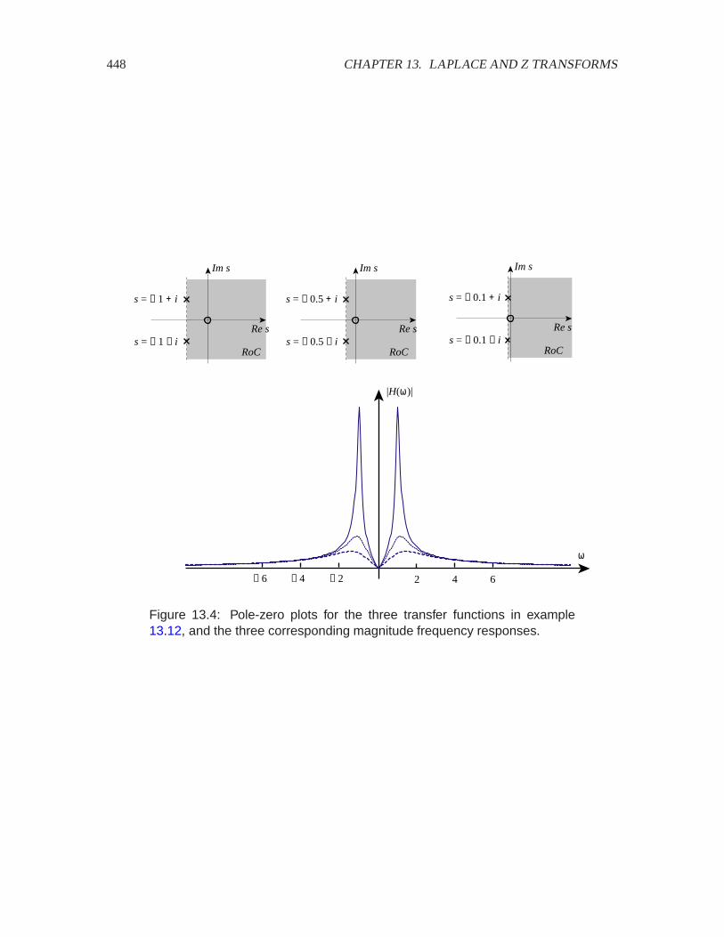
448 CHAPTER 13. LAPLACE AND Z TRANSFORMS
Im s
Re s
RoC
s = − 1 + i
2 4 6− 2− 4− 6
ω
|H(ω)|
s = − 1 − i
Im s
Re s
RoC
s = − 0.5 + i
s = − 0.5 − i
Im s
Re s
RoC
s = − 0.1 + i
s = − 0.1 − i
Figure 13.4: Pole-zero plots for the three transfer functions in example13.12, and the three corresponding magnitude frequency responses.
13.5. THE INVERSE TRANSFORMS 449
13.5 The inverse transforms
There are two inverse transforms. The inverse Z transform recovers the discrete-time signal � fromits Z transform �� . The inverse Laplace transform recovers the continuous-time signal � from itsLaplace transform �� . We study the inverse Z transform in detail. The inverse Laplace transform isalmost identical. The general approach is to break down a complicated rational polynomial into asum of simple rational polynomials whose inverse transforms we recognize. We consider only thecase where �� can be expressed as a rational polynomial.
13.5.1 Inverse Z transform
The procedure is to construct the partial fraction expansion of �� , which breaks it down into a sumof simpler rational polynomials.
Example 13.13: Consider a Z transform given by
� � RoC���� ����� �
�� � ��� � ���
�� �
�
� � �� (13.6)
This sum is called the partial fraction expansion of �� , and we will see below how tofind it systematically. We can write this as
� � RoC���� ����� � ������ � �������
where ������ � ���� � � and ������ � ��� � �� are the two terms.
To determine the inverse Z transforms of the two terms, we need to know their regionsof convergence. Recall from the linearity property that RoC��� includes the intersectionof the regions of convergence of the two terms,
RoC��� RoC���� � RoC����� (13.7)
Once we know these two regions of convergence, we can use table 13.1 to obtain theinverse Z transform of each term. By the linearity property the sum of these inverses isthe inverse Z transform of �� .
�� given by (13.6) has one pole at � � and one pole at � � �. From section 12.2.3we know that RoC��� is bordered by these poles, so it has one of three forms:
1. RoC��� � �� Complex� ��� ) ,2. RoC��� � �� Complex� ) ��� ) �, or
3. RoC��� � �� Complex� ��� 2 �.Suppose we have case (1), which implies that � is anti-causal. From (13.7), the regionof convergence of the term ���� � � must be �� Complex� ��� ) . The onlyother possibility is �� Complex� ��� 2 , which would violate (13.7) unless theintersection is empty (which would not be an interesting case). Thus, from table13.1,
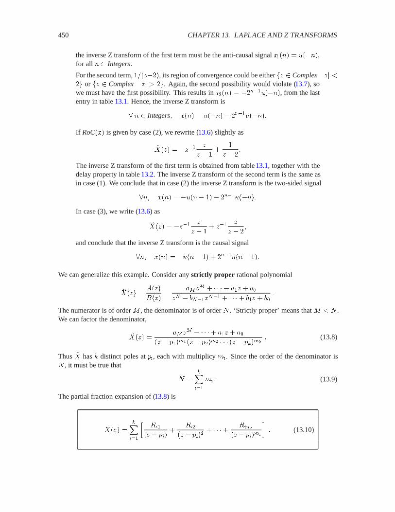
450 CHAPTER 13. LAPLACE AND Z TRANSFORMS
the inverse Z transform of the first term must be the anti-causal signal ����� � 0����,for all � Integers.
For the second term, ������, its region of convergence could be either �� Complex� ��� )� or �� Complex� ��� 2 �. Again, the second possibility would violate (13.7), sowe must have the first possibility. This results in ����� � �����0����, from the lastentry in table 13.1. Hence, the inverse Z transform is
� � Integers� ���� � 0����� ����0�����
If RoC��� is given by case (2), we rewrite (13.6) slightly as
����� � ���� �
� � �
� � ��
The inverse Z transform of the first term is obtained from table 13.1, together with thedelay property in table 13.2. The inverse Z transform of the second term is the same asin case (1). We conclude that in case (2) the inverse Z transform is the two-sided signal
��� ���� � �0��� �� ����0�����In case (3), we write (13.6) as
����� � ���� �
� � � ���
�
� � ��
and conclude that the inverse Z transform is the causal signal
��� ���� � �0��� � � ����0��� ��
We can generalize this example. Consider any strictly proper rational polynomial
����� �����
�����
���� � � ��� � ���� � �������� � � ��� � ��
�
The numerator is of order 3 , the denominator is of order � . ‘Strictly proper’ means that 3 ) � .We can factor the denominator,
����� ����� � � ��� � ��
�� � (������ � (���� �� � (����� (13.8)
Thus �� has 6 distinct poles at (�, each with multiplicy '�. Since the order of the denominator is� , it must be true that
� ���
���
'� � (13.9)
The partial fraction expansion of (13.8) is
����� ���
���
����
�� � (���
���
�� � (���� � ����
�� � (����
� (13.10)
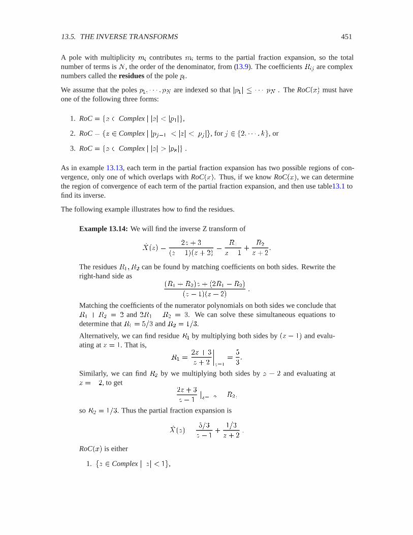
13.5. THE INVERSE TRANSFORMS 451
A pole with multiplicity '� contributes '� terms to the partial fraction expansion, so the totalnumber of terms is � , the order of the denominator, from (13.9). The coefficients ��� are complexnumbers called the residues of the pole (�.
We assume that the poles (�� � (� are indexed so that �(�� � �(� �. The RoC��� must haveone of the following three forms:
1. RoC� �� Complex� ��� ) �(��,2. RoC� �� Complex� �(���� ) ��� ) �(� �, for ��� � 6, or
3. RoC� �� Complex� ��� 2 �(�� .
As in example 13.13, each term in the partial fraction expansion has two possible regions of con-vergence, only one of which overlaps with RoC���. Thus, if we know RoC���, we can determinethe region of convergence of each term of the partial fraction expansion, and then use table13.1 tofind its inverse.
The following example illustrates how to find the residues.
Example 13.14: We will find the inverse Z transform of
����� ��� � �
�� � ��� � ���
��
� � �
��
� � ��
The residues ��� �� can be found by matching coefficients on both sides. Rewrite theright-hand side as
��� ����� � ���� ����
�� � ��� � ���
Matching the coefficients of the numerator polynomials on both sides we conclude that�� � �� � � and ��� � �� � �. We can solve these simultaneous equations todetermine that �� � ��� and �� � ��.
Alternatively, we can find residue �� by multiplying both sides by �� � � and evalu-ating at � � . That is,
�� ��� � �
� � �
####���
��
��
Similarly, we can find �� by we multiplying both sides by � � � and evaluating at� � ��, to get
�� � �
� � ����� � ���
so �� � ��. Thus the partial fraction expansion is
����� ����
� � �
��
� � ��
RoC��� is either
1. �� Complex� ��� ) ,
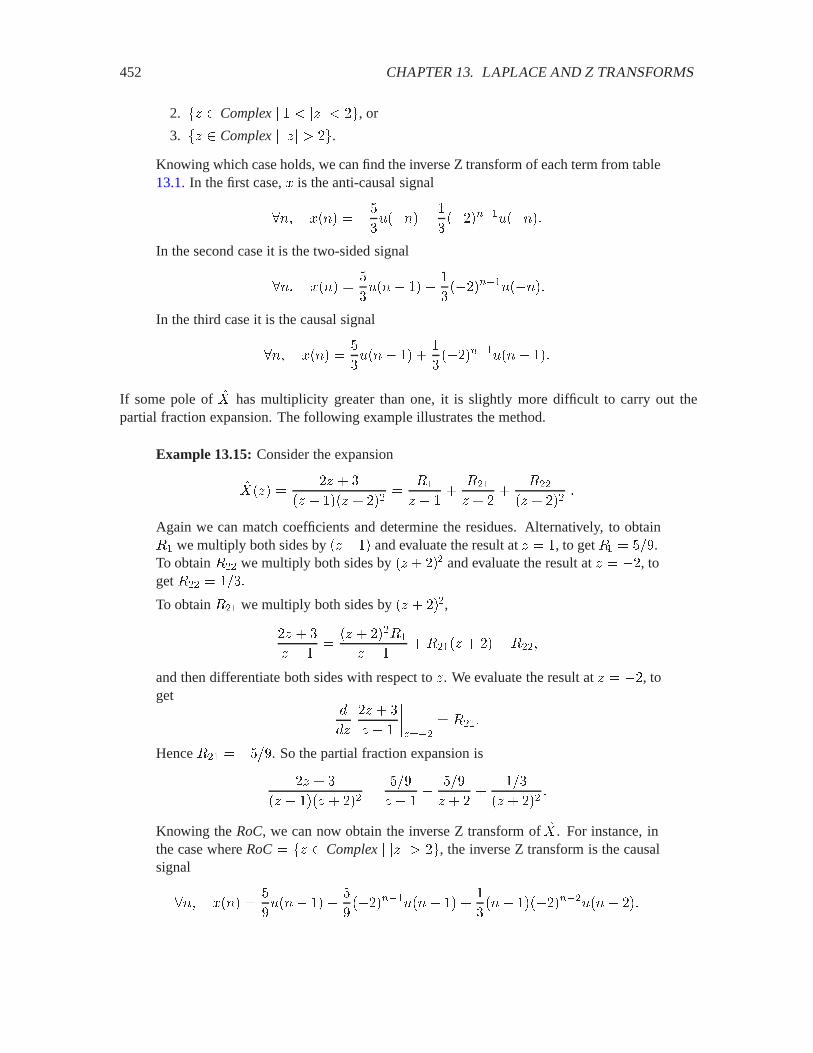
452 CHAPTER 13. LAPLACE AND Z TRANSFORMS
2. �� Complex� ) ��� ) �, or
3. �� Complex� ��� 2 �.Knowing which case holds, we can find the inverse Z transform of each term from table13.1. In the first case, � is the anti-causal signal
��� ���� � ��
�0�����
��������0�����
In the second case it is the two-sided signal
��� ���� ��
�0��� ��
��������0�����
In the third case it is the causal signal
��� ���� ��
�0��� � �
��������0��� ��
If some pole of �� has multiplicity greater than one, it is slightly more difficult to carry out thepartial fraction expansion. The following example illustrates the method.
Example 13.15: Consider the expansion
����� ��� � �
�� � ��� � ����
��
� � �
���
� � ��
���
�� � ����
Again we can match coefficients and determine the residues. Alternatively, to obtain�� we multiply both sides by ���� and evaluate the result at � � , to get �� � ���.To obtain ��� we multiply both sides by �� � ��� and evaluate the result at � � ��, toget ��� � ���
To obtain ��� we multiply both sides by �� � ���,
�� � �
� � �
�� � �����
� � ������ � �� �����
and then differentiate both sides with respect to �. We evaluate the result at � � ��, toget
�
��
�� � �
� �
####����
� ����
Hence ��� � ����. So the partial fraction expansion is
�� � �
�� � ��� � ����
���
� � � ���
� � ��
��
�� � ����
Knowing the RoC, we can now obtain the inverse Z transform of �� . For instance, inthe case where RoC� �� Complex� ��� 2 �, the inverse Z transform is the causalsignal
��� ���� ��
�0��� �� �
��������0��� � �
���� ��������0��� ���
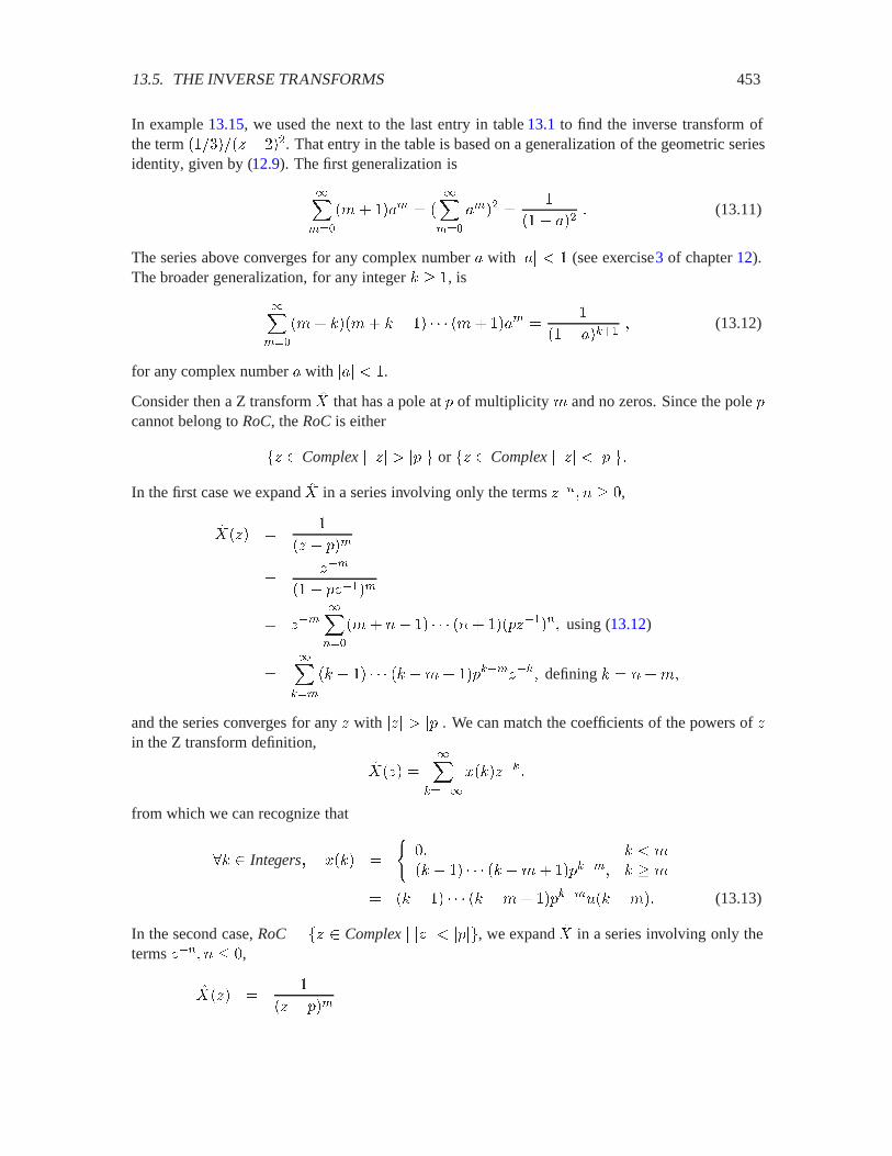
13.5. THE INVERSE TRANSFORMS 453
In example 13.15, we used the next to the last entry in table 13.1 to find the inverse transform ofthe term ������� ����. That entry in the table is based on a generalization of the geometric seriesidentity, given by (12.9). The first generalization is
�����
�'� ��� � ���
���
���� �
�� ���� (13.11)
The series above converges for any complex number � with ��� ) (see exercise3 of chapter 12).The broader generalization, for any integer 6 � , is
�����
�'� 6��'� 6 � � �'� ��� �
�� ������ (13.12)
for any complex number � with ��� ) .
Consider then a Z transform �� that has a pole at ( of multiplicity ' and no zeros. Since the pole (cannot belong to RoC, the RoCis either
�� Complex� ��� 2 �(� or �� Complex� ��� ) �(��
In the first case we expand �� in a series involving only the terms ���� � � ,
����� �
�� � (��
����
�� (�����
� ��������
�'� �� � ��� ��(������ using (13.12)
���
���
�6 � � �6 �'� �(������� defining 6 � ��'�
and the series converges for any � with ��� 2 �(�. We can match the coefficients of the powers of �in the Z transform definition,
����� ���
����
��6�����
from which we can recognize that
�6 Integers� ��6� �
�� 6 ) '�6 � � �6 �'� �(���� 6 � '
� �6 � � �6 �'� �(���0�6 �'�� (13.13)
In the second case, RoC� �� Complex� ��� ) �(�, we expand �� in a series involving only theterms ���� � � ,
����� �
�� � (��

454 CHAPTER 13. LAPLACE AND Z TRANSFORMS
�
��(��
�� (�����
�
��(�������
�'� �� � ��� ��(������ using (13.12)
� ������
����
�'� 6 � � �� 6�(������� defining 6 � ���
and the series converges for any � with ��� ) �(�. Again, we match powers of � in the Z transformdefinition to get
�6 Integers� ��6� �
������'� � 6� �� 6�(���� 6 � � 6 2
� �����'� � 6� �� 6�(���0��6�� (13.14)
Example 13.16: Suppose����� �
�� � ���
with RoC� �� Complex� ��� 2 �. Then, by (13.13), �� is the Z transform of thesignal
�6 Integers� ��6� �
�� 6 ) ��6 � ������ 6 � �
�
Suppose�$ ��� �
�� � ���
with RoC� �� Complex� ��� ) �. Then, by (13.14), �$ is the Z transform of thesignal
�6 Integers� ��6� �
��� 6������ 6 � � 6 2
�
Since the unit circle �� Complex� ��� � � RoC, the DTFT of � is defined andgiven by
�� Reals� $ ��� � �$ ����� �
���� � ����
Now that we know how to inverse transform all the terms of the partial fraction expansion, we cangeneralize the method used in example 13.15 to calculate the inverse Z transform of any �� of theform
����� ����� � � ��
�� � �������� � � ���
Step 1 If 3 � � , divide through to obtain
����� � !������� � � !� � �7 ����

13.5. THE INVERSE TRANSFORMS 455
where �7 is strictly proper.
Step 2 Carry out the partial fraction expansion of �7 and, knowing the RoC, obtain the inverse Ztransform /. Then from Table 13.1,
��� ���� � !�� �����'� , ��� � � !���� �/����
Example 13.17: We follow the procedure for
����� ��� � � � � ���
�� � ����
First, to get this into the proper form, as a rational polynomial in �, notice that
����� � ��� �$ ����
where
�$ ��� ��� � �� � � �
�� � ����
Since ��� corresponds to a one-step delay,
���� � ���� ��
so if we find the inverse Z transform of �$ , then we have found the inverse Z trasformof �� .
Working now with �$ , step 1 yields
�$ ��� � � � � ��� � �
�� � �� � ��
Step 2 gives
�7 ��� ��� � �
�� � ����
���� � ���
��
� � ��
Suppose RoC� �� Complex� ��� 2 �. Then from Table 13.1,
��� /��� � ����� ��������0��� �� � ���� ��������0��� ��
��� ���� � ��� �� ���� � /����
��� ���� � ���� ��
Hence, for all � Integers,
���� � ���� ���� �� ���� ���������0��� �� � ���� ���������0��� ���
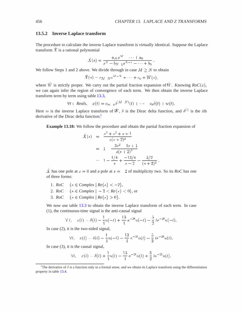
456 CHAPTER 13. LAPLACE AND Z TRANSFORMS
13.5.2 Inverse Laplace transform
The procedure to calculate the inverse Laplace transform is virtually identical. Suppose the Laplacetransform �� is a rational polynomial
����� ����� � � ��
�� � �������� � � ���
We follow Steps 1 and 2 above. We divide through in case 3 � � to obtain
����� � !������� � � !� � �7 ����
where �7 is strictly proper. We carry out the partial fraction expansion of �7 . Knowing RoC���,we can again infer the region of convergence of each term. We then obtain the inverse Laplacetransform term by term using table 13.3,
� Reals� ��� � !���Æ ������ � � !�Æ�� � /���
Here / is the inverse Laplace transform of �7 , Æ is the Dirac delta function, and Æ �� is the &thderivative of the Dirac delta function.1
Example 13.18: We follow the procedure and obtain the partial fraction expansion of
����� ��� � �� � ��
���� ���
� ����� � ���
���� ���
� ���
�������� �
����
��� ����
�� has one pole at � � and a pole at � � �� of multiplicity two. So its RoChas oneof three forms:
1. RoC� �� Complex� Re�� ) ��,2. RoC� �� Complex� � � ) Re�� ) , or
3. RoC� �� Complex� Re�� 2 .We now use table 13.3 to obtain the inverse Laplace transform of each term. In case(1), the continuous-time signal is the anti-causal signal
� � ��� � ���
�0��� � �
�����0���� �
�����0����
In case (2), it is the two-sided signal,
�� ��� � ���
�0���� �
�����0�� �
�
�����0���
In case (3), it is the causal signal,
�� ��� � �� �
�0��� �
�����0�� �
�
�����0���
1The derivative of Æ is a function only in a formal sense, and we obtain its Laplace transform using the differentiationproperty in table 13.4.
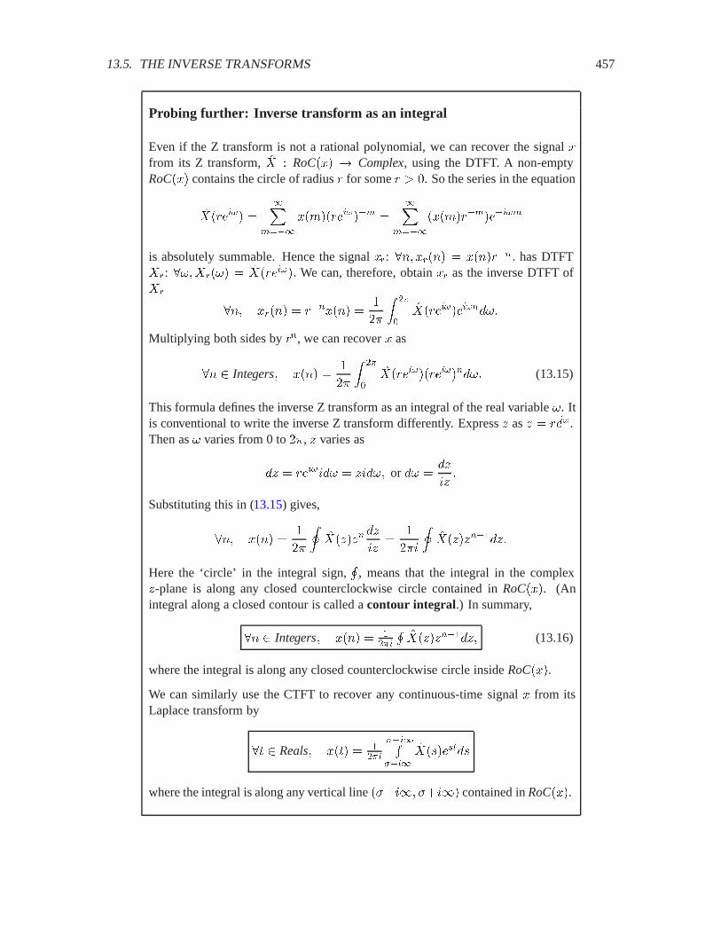
13.5. THE INVERSE TRANSFORMS 457
Probing further: Inverse transform as an integral
Even if the Z transform is not a rational polynomial, we can recover the signal �from its Z transform, �� � RoC��� � Complex, using the DTFT. A non-emptyRoC��� contains the circle of radius � for some � 2 . So the series in the equation
�������� ���
����
��'��������� ���
����
���'����������
is absolutely summable. Hence the signal �!: ��� �!��� � �������� has DTFT�!: ����!��� � ��������� We can, therefore, obtain �! as the inverse DTFT of�!
��� �!��� � ������� �
��
� �)
�
���������������
Multiplying both sides by ��, we can recover � as
�� Integers� ���� �
��
� �)
�
������������������ (13.15)
This formula defines the inverse Z transform as an integral of the real variable �. Itis conventional to write the inverse Z transform differently. Express � as � � ����.Then as � varies from 0 to ��, � varies as
�� � ����&�� � �&��� or �� ���
&��
Substituting this in (13.15) gives,
��� ���� �
��
*�������
��
&��
��&
*������������
Here the ‘circle’ in the integral sign,+
, means that the integral in the complex�-plane is along any closed counterclockwise circle contained in RoC���. (Anintegral along a closed contour is called a contour integral.) In summary,
�� Integers� ���� � ��)�
+������������ (13.16)
where the integral is along any closed counterclockwise circle inside RoC���.
We can similarly use the CTFT to recover any continuous-time signal � from itsLaplace transform by
� Reals� ��� � ��)�
4���"4���
����������
where the integral is along any vertical line �@�&�� @�&�� contained in RoC���.
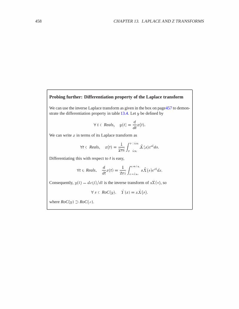
458 CHAPTER 13. LAPLACE AND Z TRANSFORMS
Probing further: Differentiation property of the Laplace transform
We can use the inverse Laplace transform as given in the box on page457 to demon-strate the differentiation property in table 13.4. Let � be defined by
� Reals� ��� ��
�����
We can write � in terms of its Laplace transform as
� Reals� ��� �
��&
� 4���
4���
�����������
Differentiating this with respect to is easy,
� Reals��
���� �
��&
� 4���
4���� �����������
Consequently, ��� � ������ is the inverse transform of � �����, so
� � RoC���� �$ ��� � � ������
where RoC��� RoC���.
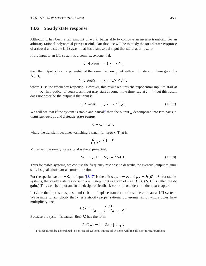
13.6. STEADY STATE RESPONSE 459
13.6 Steady state response
Although it has been a fair amount of work, being able to compute an inverse transform for anarbitrary rational polynomial proves useful. Our first use will be to study the stead-state responseof a causal and stable LTI system that has a sinusoidal input that starts at time zero.
If the input to an LTI system is a complex exponential,
� Reals� ��� � �����
then the output � is an exponential of the same frequency but with amplitude and phase given by;���,
� Reals� ��� � ;��������
where ; is the frequency response. However, this result requires the exponential input to start at � ��. In practice, of course, an input may start at some finite time, say at � , but this resultdoes not describe the output if the input is
� Reals� ��� � ����0��� (13.17)
We will see that if the system is stable and causal,2 then the output � decomposes into two parts, atransient output and a steady state output,
� � ��! � ����
where the transient becomes vanishingly small for large . That is,
!����
��!�� � �
Moreover, the steady state signal is the exponential,
�� ����� � ;�������0��� (13.18)
Thus for stable systems, we can use the frequency response to describe the eventual output to sinu-soidal signals that start at some finite time.
For the special case � � , the input (13.17) is the unit step, � � 0, and ��� � ;��0. So for stablesystems, the steady state response to a unit step input is a step of size ;��. (;�� is called the dcgain.) This case is important in the design of feedback control, considered in the next chapter.
Let � be the impulse response and �; be the Laplace transform of a stable and causal LTI system.We assume for simplicity that �; is a strictly proper rational polynomial all of whose poles havemultiplicity one,
�;��� �����
��� (�� ��� (� ��
Because the system is causal, RoC��� has the form
RoC��� � �� � Re�� 2 8�2This result can be generalized to non-causal systems, but causal systems will be sufficient for our purposes.

460 CHAPTER 13. LAPLACE AND Z TRANSFORMS
where 8 is the largest real part of any pole. Since the system is stable, 8 ) , so that the region ofconvergence includes the imaginary axis.
From table 13.3 the Laplace transform �� of the signal (13.17) is
����� �
�� &��
with RoC��� � �� Complex� Re�� 2 .The Laplace transform of the output � � � � � is
�$ � �; ���
withRoC��� RoC��� � RoC��� � �� Complex� Re�� 2 �
The partial fraction expansion of �$ is
�$ ��� � �;��� ����� �����
��� (�� ��� (� �
�� &�(13.19)
���
�� (�� � ��
�� (��
��
�� &�� (13.20)
Because everything is causal, each term must be causal, so from table13.3 we obtain
�� ��� ������
���#��0�� ����
���0���
We decompose � � ��! � ���, with
�� ��!�� ������
���#��0���
�� ����� � ������0���
Since Re�(� ) for 6 � � � � ,
!����
��!�� � �
Thus, the steady-state response ��� is eventually all that is left.
Finally, the residue �� is obtained by multiplying both sides of (13.19) by �� &� and evaluating at� � &� to get �� � �;�&�� � ;���� so that
�� ����� � ;�������0���
This analysis reveals several interesting features of the total response �. First, from (13.20) we seethe poles (�� � (� of the transfer function contribute to the transient response ��!, and the pole of

13.7. SUMMARY 461
the input �� at &� contributes to the steady state response. Second we can determine how quicklythe transient response dies down. The transient response is
�� ��!�� � ���#��0�� � ����
#� �0���
The magnitude of the terms is
�����Re�#���� � ��� ��Re�#����
Each term decreases exponentially with , since the real parts of the poles are negative. The slowestdecrease is due to the pole with the least negative part. Thus the pole of the stable, causal transferfunction with the least negative part determines how fast the transient response goes to zero. Indeedfor large , we can approximate the response � as
��� � ���#�� �;��������
where (� is the pole with the largest (least negative) real part.
There is a similar result for discrete-time systems, and it is obtained in the same way. Suppose anexponential input
�� Integers� ���� � ����0����
is applied to a stable and causal system with impulse response �, transfer function �; , and frequencyresponse ; . Then the output � � � � � can again be decomposed as
��� ���� � ��!��� � �������
where the transient ��!���� as ���, and the steady state response is
��� ������ � �;���������0��� � ;�������0����
For large �, the transient response decays exponentially as (�� , i.e.
���� � ��(�� � �������
where (� is the pole with the largest magnitude (which must be less than one, since the system isstable).
13.7 Summary
The Z transform and Laplace transform have many of the same properties as the Fourier trans-forms. They are linear, which greatly facilitates computation of the transforms and their inverses.Moreover, the Z transform (Laplace transform) of the output of an LTI system is the product ofthe Z transforms (Laplace transforms) of the input and the transfer function. Thus, the Z trans-form (Laplace transform) plays the same role as the frequency response, describing the relationshipbetween the input and the output as a product rather than a convolution.
462 CHAPTER 13. LAPLACE AND Z TRANSFORMS
Exercises
Each problem is annotated with the letter E, T, C which stands for exercise, requires some thought,requires some conceptualization. Problems labeled E are usually mechanical, those labeled T re-quire a plan of attack, those labeled C usually have more than one defensible answer.
1. E Consider the signal � given by
��� ���� � ��������0����
(a) Show that the Z transform is
� � RoC���� ����� �� �������
�� � �� ������� � �
whereRoC��� � �� Complex� ��� 2 �
(b) Where are the poles and zeros?
(c) Is � absolutely summable?
2. T Consider the signal � given by
� � Integers� ���� � �����
where � Complex.
(a) Find the Z transform of �. Be sure to give the region of convergence.
(b) Where are the poles?
(c) Under what conditions is � absolutely summable?
3. E Consider a discrete-time LTI system with transfer function given by
� � �� � ��� 2 ��� �;��� ��
� � ���
Suppose that the input � is given by
� � Integers� ���� � ���� ���� � ��
Find the Z transform of the output �, including its region of convergence.
4. E Consider the exponentially modulated sinusoid � given by
� � Integers� ���� � �� ��������0����
where � is a real number, �� is a real number, and 0 is the unit step signal.
(a) Find the Z transform. Be sure to give the region of convergence. Hint: Use example13.3 and section 13.1.6.
13.7. SUMMARY 463
(b) Where are the poles?
(c) For what values of � is this signal absolutely summable?
5. T Suppose � DiscSignalssatisfies
������
��������� )�� ) �� ) � ) ���
for some real numbers �� and �� such that �� ) ��. Show that
������
���������� )�� ) �� ) � ) ���
Hint: Use the fact that for any A 2 there exists � ) � such that �� � A��� ) for all� 2 � .
6. T Consider a causal discrete-time LTI system where the input � and output � are related bythe difference equation
� � Integers� ���� � ������ � � ������ �� � ������ � ������ � � ������ ���
where ��, ��, ��, ��, and �� are real-valued constants.
(a) Find the transfer function.
(b) Say as much as you can about the region of convergence.
(c) Under what conditions is the system stable?
7. E This exercise verifies the time delay property of the Laplace transform. Show that if � is acontinuous-time signal, � is a real constant, and � is given by
� Reals� ��� � ��� ���
then its Laplace transform is
� � RoC���� �$ ��� � ���( ������
with region of convergenceRoC��� � RoC����
8. E This exercise verifies the convolution property of the Laplace transform. Suppose � and �have Laplace transforms �� and �; . Let � be given by
� Reals� ��� � �� � ���� ���
��
������� �����
Then show that the Laplace transform is
�� RoC���� �$ ��� � ����� �;����
withRoC��� RoC��� � RoC����
464 CHAPTER 13. LAPLACE AND Z TRANSFORMS
9. T This exercise verifies the conjugation property of the Laplace transform, and then usesthis property to demonstrate that for real-valued signals, poles and zeros come in complex-conjugate pairs.
(a) Let � be a complex-valued continuous-time signal and � be given by
� Reals� ��� � �������
Show that� � RoC���� �$ ��� � � ���������
whereRoC��� � RoC����
(b) Use this property to show that if � is real, then complex poles and zeros occur in complexconjugate pairs. That is, if there is a zero at � � 8, then there must be a zero at � � 8�,and if there is a pole at � � (, then there must also be a pole at � � (�.
10. T This exercise verifies the time scaling property of the Laplace transform. Let � be definedby
� Reals� ��� � ��!��
for some real number !. Show that
� � RoC���� �$ ��� � �����!���!��
whereRoC��� � �� � ��! RoC����
11. E This exercise verifies the exponential scaling property of the Laplace transform. Let � bedefined by
� Reals� ��� � �������
for some complex number �. Show that
� � RoC���� �$ ��� � ����� ���
whereRoC��� � �� � �� � RoC����
12. T Consider a discrete-time LTI system with impulse response
��� ���� � �� ��������0����
for some �� Reals. Show that if the input is
� � Integers� ���� � �����0����
then the output � is unbounded.

13.7. SUMMARY 465
13. E Find and plot the inverse Z transform of
����� �
�� � ���
with
(a) Roc��� � �� Complex� ��� 2 �(b) Roc��� � �� Complex� ��� ) �.
14. E Obtain the partial fraction expansions of the following rational polynomials. First dividethrough if necessary to get a strictly proper rational polynomial.
(a)
� � �
�� � ��� � ��
(b)
�� � ���
�� � ��� � ��
(c)
� � �
�� � ��
15. E Find the inverse Z transform � for each of the three possible regions of convergence asso-ciated with
����� ��� � ���
�� � ��� � ���
For which region of convergence is � causal? For which is � strictly anti-causal? For whichis � two-sided?
16. E Find the inverse Z transform � for each of the two possible regions of convergence associ-ated with
����� �� � �
�� � ��
17. E Consider a stable system with impulse response
���� � ����������
Find the steady-state response to a unit step input.
18. E Let ���� � ��0����, all �, and ���� � ���0���, for all �. Find � � 0 and � � 0, where 0is the unit step.
19. This exercise shows how we can determine the transfer function and frequency response of anLTI system from its step response. Suppose a causal system with step input � � 0, producesthe output
� � Integers� ���� � �� ����0����
466 CHAPTER 13. LAPLACE AND Z TRANSFORMS
(a) Find the transfer function (including its region of convergence).
(b) If the system is stable, find its frequency response.
(c) Find the impulse response of the system.
20. Consider an LTI system with impulse response � given by
� � Integers� ���� � ��0����
(a) Find the transfer function, including its region of convergence.
(b) Use the transfer function to find the Z transform of the step response.
(c) Find the inverse transform of the result of part (b) to obtain the step response in the timedomain.
Chapter 14
Composition and Feedback Control
A major theme of this book is that interesting systems are often compositions of simpler systems.Systems are functions, so their composition is function composition, as discussed in section2.1.5.However, systems are often not directly described as functions, so function composition is not theeasiest tool to use to understand the composition. We have seen systems described as state machines,frequency responses, and transfer functions. In chapter4 we obtained the state machine of the com-posite system from its component state machines. In section8.5 we obtained the frequency responseof the composite system from the frequency response of its component linear time-invariant (LTI)systems. We extend the latter study in this chapter to the composition of LTI systems describedby their transfer functions. This important extension allows us to consider unstable systems whoseimpulse response has a Z or Laplace transform, but not a Fourier transform.
As before, feedback systems prove challenging. A particularly interesting issue is how to maintainstability, and how to construct stable systems out of unstable ones. We will find that some feedbackcompositions of stable systems result in unstable systems, and conversely, some compositions ofunstable systems result in stable systems. For example, we can stabilize the helicopter in example12.2 using feedback, in fact we can precisely control its orientation, despite the intrinsic instability.The family of techniques for doing this is known as feedback control. This chapter serves as anintroduction to that topic. Feedback control can also be used to drive stable systems, in whichcase it serves to improve their response. For example, feedback can result in faster or more preciseresponses, and can also prevent overshoot, where a system overreacts to a command.
We will consider three styles of composition, cascade composition, parallel composition, andfeedback composition. In each case, two LTI systems with transfer functions �;� and �;� arecombined to get a new system. The transfer functions �;� and �;� are the (Z or Laplace) transformsof the respective impulse responses, �� and ��. Much of our discussion applies equally well whetherthe system is a continuous-time system or a discrete-time system, so in many cases we leave thisunspecified.
467
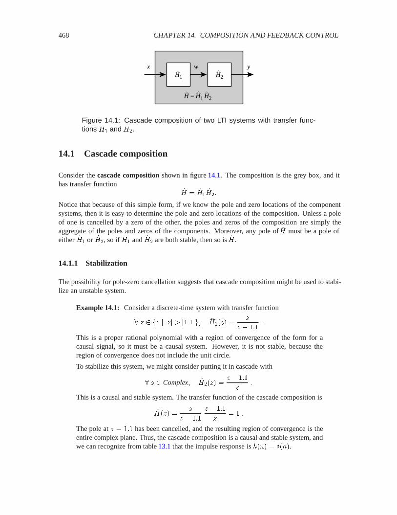
468 CHAPTER 14. COMPOSITION AND FEEDBACK CONTROL
H1
x wH2
y
H = H1 H2
Figure 14.1: Cascade composition of two LTI systems with transfer func-tions ;� and ;�.
14.1 Cascade composition
Consider the cascade composition shown in figure 14.1. The composition is the grey box, and ithas transfer function
�; � �;��;��
Notice that because of this simple form, if we know the pole and zero locations of the componentsystems, then it is easy to determine the pole and zero locations of the composition. Unless a poleof one is cancelled by a zero of the other, the poles and zeros of the composition are simply theaggregate of the poles and zeros of the components. Moreover, any pole of �; must be a pole ofeither �;� or �;�, so if �;� and �;� are both stable, then so is �; .
14.1.1 Stabilization
The possibility for pole-zero cancellation suggests that cascade composition might be used to stabi-lize an unstable system.
Example 14.1: Consider a discrete-time system with transfer function
� � �� � ��� 2 ���� �;���� ��
� � ��
This is a proper rational polynomial with a region of convergence of the form for acausal signal, so it must be a causal system. However, it is not stable, because theregion of convergence does not include the unit circle.
To stabilize this system, we might consider putting it in cascade with
� � Complex� �;���� �� � �
��
This is a causal and stable system. The transfer function of the cascade composition is
�;��� ��
� � �
� � �
�� �
The pole at � � � has been cancelled, and the resulting region of convergence is theentire complex plane. Thus, the cascade composition is a causal and stable system, andwe can recognize from table 13.1 that the impulse response is ���� � ���.
14.1. CASCADE COMPOSITION 469
Stabilizing systems by cancelling their poles in a cascade composition, however, is almost never agood idea. If the pole is not precisely cancelled, then no matter how small the error, the resultingsystem is still unstable.
Example 14.2: Suppose that in the previous example the pole location is not knownprecisely, and turns out to be at � � � instead of � � �. Then the cascadecomposition has transfer function
�;��� ��
� � �
� � �
��
� � �
� � ��
which is unstable.
14.1.2 Equalization
While cascade compositions do not usually work well for stabilization, they do often work well forequalization. An equalizer is a compensator that reverses distortion. The source of the distortion,which is often called a channel, must be an LTI system, and the equalizer is composed in cascadewith it. At first sight this is easy to do. If the channel has transfer function �;�, then the equalizercould have transfer function
�;� � �;��� �
in which case the cascade composition will have transfer function
�; � �;��;� � �
which is certainly distortion-free.
Example 14.3: Some acoustic environments for audio have resonances, where certainfrequencies are enhanced as the sound propagates through the environment (see labC.8for an example). This will typically occur if the physics of the acoustic environmentresults in a transfer function with poles near the unit circle (for a discrete-time model)or near the imaginary axis (for a continuous-time model). Suppose for example thatthe acoustic environment is well modeled by a discrete-time LTI system with transferfunction
� � �� � ��� 2 ���� �;���� ���
�� � ���� � ����
where � � ������� for some frequency ��. Using the methods of section 13.2, we caninfer that the magnitude response will have a strong peak at frequencies �� and ���,because the positions on the unit circle ���� and ����� are very close to the poles. Thiswill result in distortion of the audio signal, where frequencies near �� will be amplified.
An equalizer that will compensate for this distortion has transfer function
�;���� � � �;������� �
�� � ���� � ���
���
�� � �Re��� � ������
�
470 CHAPTER 14. COMPOSITION AND FEEDBACK CONTROL
As in example 13.2, we can recognize this as the Z transform of an FIR filter withimpulse response
� � Integers� ����� � ��� � �Re���� � � � ������� ���
This filter is causal and stable, and hence can serve as an effective equalizer.
There are a number of potential problems with this approach, however. First, the transfer functionof the channel is probably not known, or at least not known precisely. Second, the channel may nothave a stable and causal inverse.
Let us first examine the first difficulty, that the channel may not be known (precisely). If the channelmodel �;� and its inverse �;� are both stable, then the cascade composition is at least assured ofbeing stable, even if the channel has been misconstrued. Moreover, if the equalizer is close to theinverse of the true channel, then often the distortion is significantly reduced despite the errors (seeexercise 1).
This difficulty can sometimes be dealt with by adaptively varying the equalizer based on measure-ments of the distortion. One way to measure the distortion is to send through the channel a knownsequence called a training sequence and observe the output of the channel. Suppose that the train-ing sequence is a signal � with Z transform �� , and that the channel �;� is unknown. If we canobserve the output � of the channel, and calculate its Z transform �$ , then the channel transferfunction is simply
� � RoC����� �;���� ��$ ���
������
where RoC���� is determined by identifying the poles and zeros of the rational polynomial�$ ���� �����and finding the one ring-shaped region that includes the unit circle and is bordered by poles. Thisresults in a stable channel model.
Training sequences are commonly used in digital communication systems, where, for example, aradio channel introduces distortion. However, it is also common for such channels to change overtime. Radio channels, for example, change if either the transmitter or receiver moves, or if theweather changes, or if obstacles appear or disappear. Repeatedly transmitting training sequences isan expensive waste of radio bandwidth, and fortunately, is not usually necessary, as illustrated in thefollowing example.
Example 14.4: Consider a digital communication system where the channel is mod-eled as a discrete-time LTI system with transfer function �;�, representing for examplea radio transmission subsystem. Suppose that this digital communication system trans-mits a bit sequence represented as a discrete-time signal � of form
�� Integers� �� �Suppose further that we use a training sequence to obtain an initial estimate �;� of theinverse of the channel. But over time, the channel drifts, so that �;� is no longer theinverse of �;�. Assuming the drift is relatively slow, then after a short time, �;� is stillclose to the inverse of �;�, in that the cascade �;�
�;� yields only mild distortion. That
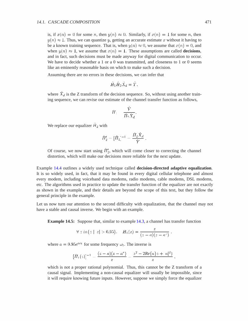
14.1. CASCADE COMPOSITION 471
is, if ���� � for some �, then ���� � . Similarly, if ���� � for some �, then���� � . Thus, we can quantize �, getting an accurate estimate � without it having tobe a known training sequence. That is, when ���� � , we assume that ���� � , andwhen ���� � , we assume that ���� � . These assumptions are called decisions,and in fact, such decisions must be made anyway for digital communication to occur.We have to decide whether a 1 or a 0 was transmitted, and closeness to 1 or 0 seemslike an eminently reasonable basis on which to make such a decision.
Assuming there are no errors in these decisions, we can infer that
�;��;�
��% � �$ �
where ��% is the Z transform of the decision sequence. So, without using another train-ing sequence, we can revise our estimate of the channel transfer function as follows,
�;� ��$
�;���%
�
We replace our equalizer �;� with
�; �� � � �;��
�� ��;�
��%
�$�
Of course, we now start using �; ��, which will come closer to correcting the channel
distortion, which will make our decisions more reliable for the next update.
Example 14.4 outlines a widely used technique called decision-directed adaptive equalization.It is so widely used, in fact, that it may be found in every digital cellular telephone and almostevery modem, including voiceband data modems, radio modems, cable modems, DSL modems,etc. The algorithms used in practice to update the transfer function of the equalizer are not exactlyas shown in the example, and their details are beyond the scope of this text, but they follow thegeneral principle in the example.
Let us now turn our attention to the second difficulty with equalization, that the channel may nothave a stable and causal inverse. We begin with an example.
Example 14.5: Suppose that, similar to example 14.3, a channel has transfer function
� � &��� � ��� 2 ���� �;���� ��
�� � ���� � ����
where � � ������� for some frequency ��. The inverse is
� �;������� �
�� � ���� � ���
��
�� � �Re��� � ������
�
which is not a proper rational polynomial. Thus, this cannot be the Z transform of acausal signal. Implementing a non-causal equalizer will usually be impossible, sinceit will require knowing future inputs. However, suppose we simply force the equalizer
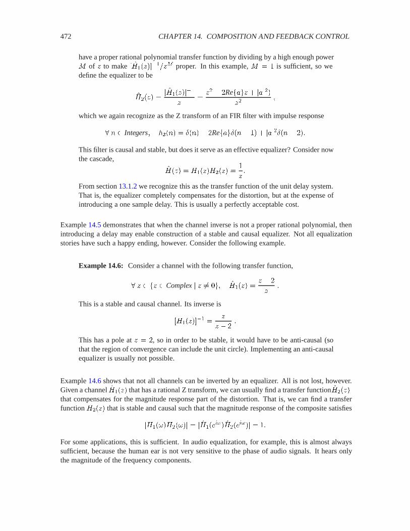
472 CHAPTER 14. COMPOSITION AND FEEDBACK CONTROL
have a proper rational polynomial transfer function by dividing by a high enough power3 of � to make � �;�����
����� proper. In this example, 3 � is sufficient, so wedefine the equalizer to be
�;���� �� �;�����
��
��
�� � �Re��� � �������
�
which we again recognize as the Z transform of an FIR filter with impulse response
� � Integers� ����� � ��� � �Re���� � � � ������� ���
This filter is causal and stable, but does it serve as an effective equalizer? Consider nowthe cascade,
�;��� � �;���� �;���� �
��
From section 13.1.2 we recognize this as the transfer function of the unit delay system.That is, the equalizer completely compensates for the distortion, but at the expense ofintroducing a one sample delay. This is usually a perfectly acceptable cost.
Example 14.5 demonstrates that when the channel inverse is not a proper rational polynomial, thenintroducing a delay may enable construction of a stable and causal equalizer. Not all equalizationstories have such a happy ending, however. Consider the following example.
Example 14.6: Consider a channel with the following transfer function,
� � �� Complex� � �� � �;���� �� � �
��
This is a stable and causal channel. Its inverse is
� �;������� �
�
� � ��
This has a pole at � � �, so in order to be stable, it would have to be anti-causal (sothat the region of convergence can include the unit circle). Implementing an anti-causalequalizer is usually not possible.
Example 14.6 shows that not all channels can be inverted by an equalizer. All is not lost, however.Given a channel �;���� that has a rational Z transform, we can usually find a transfer function �;����that compensates for the magnitude response part of the distortion. That is, we can find a transferfunction �;���� that is stable and causal such that the magnitude response of the composite satisfies
�;����;����� � � �;������ �;���
���� � �
For some applications, this is sufficient. In audio equalization, for example, this is almost alwayssufficient, because the human ear is not very sensitive to the phase of audio signals. It hears onlythe magnitude of the frequency components.

14.2. PARALLEL COMPOSITION 473
Example 14.7: Continuing example 14.6, let �;� be given by
�;� ��
� �������� � ��
�
This has a pole at � � ��, and is a proper rational polynomial, so it can be the transferfunction of a causal and stable filter. Consider the cascade composition,
�;��� � �;���� �;���� ��
� � � ����� � ��
�� ���
� � ���
This hardly looks like what we want, but if we rewrite it slightly, it is easy to show thatthe magnitude frequency response has value one for all �,
�;��� �� ���
� � ��� �
��� � ��
� � ���
The magnitude frequency response is
�;���� � � �;������ � ����� ����� � ������� � ��� � �
This magnitude is equal to 1 because the numerator, ���� � ��, is the complex conju-gate of the denominator, ��� � ��, so they have the same magnitude.
The method in example 14.7 can be generalized so that for most channels it is possible to cancelany magnitude distortion. The key is that if the channel transfer function has a zero outside the unitcircle, say at � � �, then its inverse has a pole at the same location, � � �. A pole outside the unitcircle makes it impossible to have a stable and causal filter. So the trick is to place a pole instead at� � ���. This pole will cancel the effect on the magnitude (but not the phase) of the zero at � � �.
There are still channels for which this method will not work.
Example 14.8: Consider a channel given by
� � �� Complex� � �� � �;���� �� �
��
This has a pole at � � and a zero at � � . Its inverse cannot be stable because itwill have a pole at � � . In fact, no equalization is possible. This is intuitive becausethe frequency response is zero at � � , and no stable equalizer in cascade with thischannel can reconstruct the original component at � � . It would have to have infinitegain at � � , which would make it unstable.
14.2 Parallel composition
Consider the parallel composition shown in figure 14.2. The transfer function of the compositionsystem is
�; � �;� � �;��

474 CHAPTER 14. COMPOSITION AND FEEDBACK CONTROL
H1
x
w1
H2
y
H = H1+ H2
w2
Figure 14.2: Parallel composition of two LTI systems with transfer functions;� and ;�.
This is valid whether these are Laplace transforms or Z transforms. Once again, notice that a poleof �; must be a pole of either �;� or �;�, so if �;� and �;� are stable, then so is �; . At the poles of�;�, �;���� is infinite, so very likely a pole of �;� will also be a pole of �; . However, just as in the
cascade composition, this pole may be cancelled by a zero.
Determining the location of the zeros of the composition, however, is slightly more complicated thanfor cascade composition. The sum has to be put into rational polynomial form, and the polynomialsthen need to be factored.
14.2.1 Stabilization
Just as with cascade composition, stabilizing systems by cancelling their poles in a parallel compo-sition is possible, but is almost never a good idea.
Example 14.9: Consider a discrete-time system with transfer function
� � �� � ��� 2 ���� �;���� ��
� � ��
This describes a causal but unstable system. Suppose we combine this in parallel witha system with transfer function
� � �� � ��� 2 ���� �;���� ���� � �
�
This is again causal and unstable. The transfer function of the parallel composition is
�;��� ��
� � ��
��� � �
�� � �
� � �� �
The pole at � � � has been cancelled, and the resulting region of convergence is theentire complex plane. Thus, the parallel composition is a causal and stable system withimpulse response ���� � ���.

14.2. PARALLEL COMPOSITION 475
H1
x
w
H2
y
w1
w2
Figure 14.3: Structure of a noise canceller.
However, if the pole is not precisely cancelled, then no matter how small the error, the resultingsystem is still unstable.
Example 14.10: Suppose that in the previous example the pole location is not knownprecisely, and turns out to be at � � � instead of � � �. Then the parallelcomposition has transfer function
�;��� ��
� � ��
�
� � ��
�� � ���� � �
�� � ���� � ���
which is unstable.
14.2.2 Noise cancellation
While parallel compositions do not usually work well for stabilization, with a small modificationthey do often work well for noise cancellation. A noise canceller is a compensator that removesan unwanted component from a signal. The unwanted component is called noise.
The pattern of a noise cancellation problem is shown in figure14.3. The signal � is a noise source.This signal is filtered by �;� and added to the desired signal /. The result is a noisy signal. Tocancel the noise, the signal from the noise source is filtered by a noise cancelling filter �;� and theresult is added to the noisy signal. If � has (Laplace or Z) transform �� , / has transform �7 , and �has transform �$ , then
�$ � �7 � � �;� � �;�� ���
From this it is evident that if we choose
�;� � � �;��
then � will be a clean (noise-free) signal, equal to /. The following examples describe real-worldapplications of this pattern.
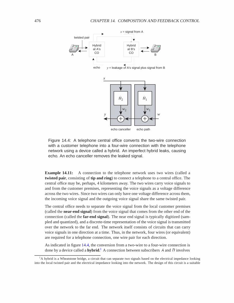
476 CHAPTER 14. COMPOSITION AND FEEDBACK CONTROL
A B
Hybridat A'sCO
Hybridat B'sCO
x = signal from A
y = leakage of A's signal plus signal from Becho
twisted pair
H1
x
w
H2
y
echo pathecho canceller
w1w2
Figure 14.4: A telephone central office converts the two-wire connectionwith a customer telephone into a four-wire connection with the telephonenetwork using a device called a hybrid. An imperfect hybrid leaks, causingecho. An echo canceller removes the leaked signal.
Example 14.11: A connection to the telephone network uses two wires (called atwisted pair, consisting of tip and ring) to connect a telephone to a central office. Thecentral office may be, perhaps, 4 kilometers away. The two wires carry voice signals toand from the customer premises, representing the voice signals as a voltage differenceacross the two wires. Since two wires can only have one voltage difference across them,the incoming voice signal and the outgoing voice signal share the same twisted pair.
The central office needs to separate the voice signal from the local customer premises(called the near-end signal) from the voice signal that comes from the other end of theconnection (called the far-end signal). The near end signal is typically digitized (sam-pled and quantized), and a discrete-time representation of the voice signal is transmittedover the network to the far end. The network itself consists of circuits that can carryvoice signals in one direction at a time. Thus, in the network, four wires (or equivalent)are required for a telephone connection, one wire pair for each direction.
As indicated in figure 14.4, the conversion from a two-wire to a four-wire connection isdone by a device called a hybrid.1 A connection between subscribers � and � involves
1A hybrid is a Wheatstone bridge, a circuit that can separate two signals based on the electrical impedance lookinginto the local twisted pair and the electrical impedance looking into the network. The design of this circuit is a suitable

14.2. PARALLEL COMPOSITION 477
two hybrids, one in each subscriber’s central office. The hybrid in �’s central officeideally will pass all of the incoming signal � to �’s two-wire circuit, and none backinto the network. However, the hybrid is not perfect, and some of the incoming signal� leaks through the hybrid into the return path back to �. The signal � in the figure isthe sum of the signal from � and the leaked signal from �. � hears the leaked signalas an echo, since it is �’s own signal, delayed by propagation through the telephonenetwork.
If the telephone connection includes a satellite link, then the delay from one end of theconnection to the other is about 300ms. This is the time it takes for a radio signal topropagate to a geosynchronous satellite and back. The echo traverses this link twice:once going from � to �, and the second time coming back. Thus, the echo is �’sown signal delayed by about 600ms. For voice signals, 600ms of delay is enough tocreate a very annoying echo that can make it difficult to speak. Humans have difficultyspeaking when they hear their own voices 600ms later. Consequently, the designers ofthe telephone network have put echo cancellers in to prevent the echo from occuring.
Let �;� be the transfer function of the hybrid leakage path. The echo canceller is thefilter �;� placed in parallel composition with the hybrid, as shown in the figure. Theoutput /� of this filter is added to the output /� � / of the hybrid, so the signal thatactually goes back is � � /� � /� � /. If
�;� � � �;��
then � � / and the echo is cancelled perfectly. Moreover, note that as long as �;� isstable and causal, so will be the echo canceller �;�.
However, �;� is not usually known in advance, and also it changes over time. So either afixed �;� is designed to match a ‘typical’ �;�, or an adaptive echo canceller is designedthat estimates the characteristics of the echo path (�;�) and changes �;� accordingly.Adaptive echo cancellers are common in the telephone network today.
The following example combines cascade and parallel composition to achieve noise cancellation.
Example 14.12: Consider a microphone in a noisy environment. For example, atraffic helicopter might be used to deliver live traffic reports over the radio, but the(considerable) background noise of the helicopter would be highly undesirable on theradio. Fortunately, the background noise can be cancelled. Referring to figure14.5,suppose that / is the announcer’s voice, � is the engine noise, and �;� represents theacoustic path from the engine noise to the microphone. The microphone picks up boththe engine noise and the announcer’s voice, producing the noisy signal /. We canplace a second microphone somewhere far enough from the announcer so as to not pickup much of his or her voice. Since this microphone is in a different place, say on theback of the announcer’s helmet, the acoustic path is different, so we model that path
topic for a text on electrical circuits.
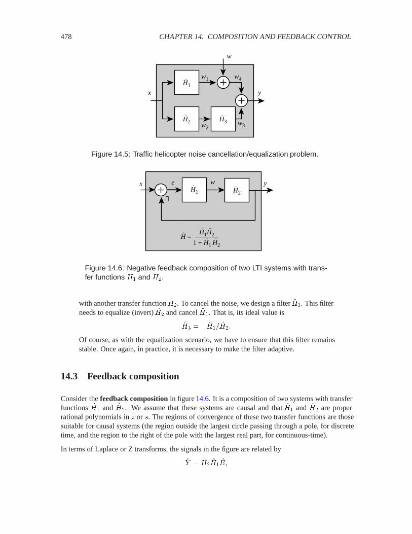
478 CHAPTER 14. COMPOSITION AND FEEDBACK CONTROL
H1
x
w
H2
y
w1
w2
H3 w3
w4
Figure 14.5: Traffic helicopter noise cancellation/equalization problem.
H1
x eH2
y
H =
w
H1H2
1 + H1 H2
−
Figure 14.6: Negative feedback composition of two LTI systems with trans-fer functions ;� and ;�.
with another transfer function �;�. To cancel the noise, we design a filter �;�. This filterneeds to equalize (invert) �;� and cancel �;�. That is, its ideal value is
�;� � � �;�� �;��
Of course, as with the equalization scenario, we have to ensure that this filter remainsstable. Once again, in practice, it is necessary to make the filter adaptive.
14.3 Feedback composition
Consider the feedback composition in figure 14.6. It is a composition of two systems with transferfunctions �;� and �;�. We assume that these systems are causal and that �;� and �;� are properrational polynomials in � or �. The regions of convergence of these two transfer functions are thosesuitable for causal systems (the region outside the largest circle passing through a pole, for discretetime, and the region to the right of the pole with the largest real part, for continuous-time).
In terms of Laplace or Z transforms, the signals in the figure are related by
�$ � �;��;�
�=�
14.3. FEEDBACK COMPOSITION 479
and�= � �� � �$ �
Notice that, by convention, the feedback term is subtracted, as indicated by the minus sign adjacentto the adder (for this reason, this composition is called negative feedback). Combining these twoequations to elimintate �=, we get
�$ � �;��;�� �� � �$ ��
which we can solve for the transfer function of the composition,
�; ��$
���
�;��;�
� �;��;�
� (14.1)
This is often called the closed-loop transfer function, to contrast it with the open-loop transferfunction, which is simply �;�
�;�. We will assume that this resulting system is causal, and that theregion of convergence of this transfer function is therefore determined by the roots of the denomi-nator polynomial, � �;�
�;�.
The closed-loop transfer function is valid as long as the denominator � �;��;� is not identically
zero (that is, it is not zero for all � or � in Complex– it may be zero some� or � in Complex). Thisis sufficient for the feedback loop to be well-formed, although in general, this fact is not trivial todemonstrate (exercise 8 considers the easier case where �;�
�;� is causal and strictly proper, in whichcase the system �;�
�;� has state-determined output). We will assume henceforth, without comment,that the denominator is not identically zero.
Feedback composition is useful for stabilizing unstable systems. In the case of cascade and parallelcomposition, a pole of the composite must be a pole of one of the components. The only way toremove or alter a pole of the components is to cancel it with a zero. For this reason, cascade and par-allel composition are not effective for stabilizing unstable systems. Any error in the specification ofthe unstable pole location results in a failed cancellation, which results in an unstable composition.
In contrast, the poles of the feedback composition are the roots of the denominator ��;��;�, which
are generally quite different from the poles of �;� and �;�. This leads to the following importantconclusion:
The poles of a feedback composition can be different from the poles of its com-ponent subsystems. Consequently, unstable system can be effectively and robustlystabilized by feedback.
The stabilization is robust in that small changes in the pole or zero locations do not result in thecomposition going unstable. We will be able to quantify this robustness.
14.3.1 Proportional controllers
In control applications, one of the two systems being composed, say �;�, is called the plant. Thisis a physical system that is given to us to control. Its transfer function is determined by its physics.
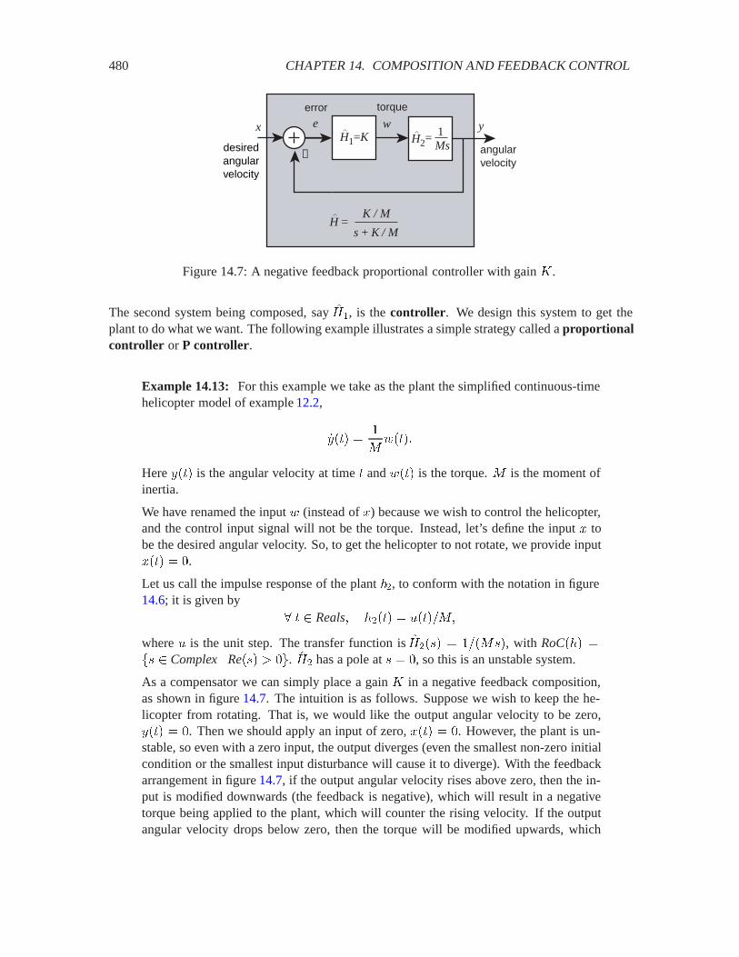
480 CHAPTER 14. COMPOSITION AND FEEDBACK CONTROL
H1=Kx e
H2
y
H =
w
K / M
s + K / M
−Ms1=
desiredangularvelocity
angularvelocity
torqueerror
Figure 14.7: A negative feedback proportional controller with gain > .
The second system being composed, say �;�, is the controller. We design this system to get theplant to do what we want. The following example illustrates a simple strategy called a proportionalcontroller or P controller.
Example 14.13: For this example we take as the plant the simplified continuous-timehelicopter model of example 12.2,
���� �
3/���
Here ��� is the angular velocity at time and /�� is the torque. 3 is the moment ofinertia.
We have renamed the input / (instead of �) because we wish to control the helicopter,and the control input signal will not be the torque. Instead, let’s define the input � tobe the desired angular velocity. So, to get the helicopter to not rotate, we provide input��� � .
Let us call the impulse response of the plant ��, to conform with the notation in figure14.6; it is given by
� Reals� ���� � 0���3�
where 0 is the unit step. The transfer function is �;���� � ��3��, with RoC��� ��� Complex� Re��� 2 . �;� has a pole at � � , so this is an unstable system.
As a compensator we can simply place a gain > in a negative feedback composition,as shown in figure 14.7. The intuition is as follows. Suppose we wish to keep the he-licopter from rotating. That is, we would like the output angular velocity to be zero,��� � . Then we should apply an input of zero, ��� � . However, the plant is un-stable, so even with a zero input, the output diverges (even the smallest non-zero initialcondition or the smallest input disturbance will cause it to diverge). With the feedbackarrangement in figure 14.7, if the output angular velocity rises above zero, then the in-put is modified downwards (the feedback is negative), which will result in a negativetorque being applied to the plant, which will counter the rising velocity. If the outputangular velocity drops below zero, then the torque will be modified upwards, which
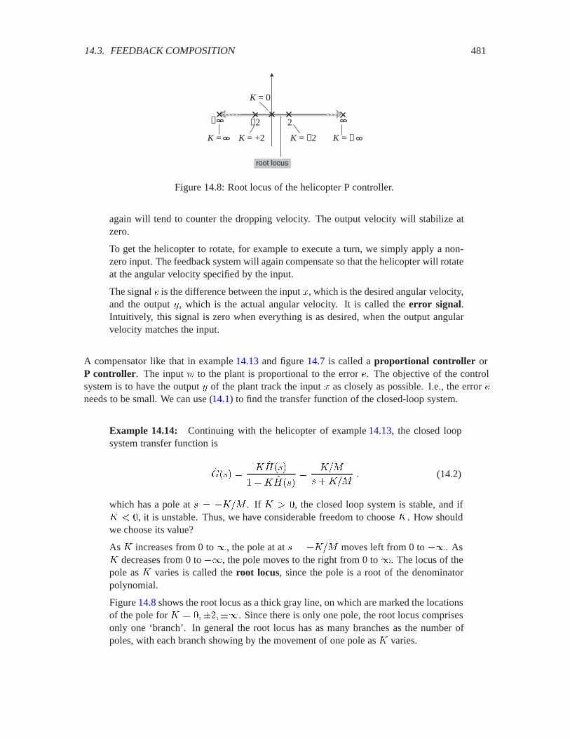
14.3. FEEDBACK COMPOSITION 481
2− −2
K = −2K = +2 K = −K =
root locus
K = 0
Figure 14.8: Root locus of the helicopter P controller.
again will tend to counter the dropping velocity. The output velocity will stabilize atzero.
To get the helicopter to rotate, for example to execute a turn, we simply apply a non-zero input. The feedback system will again compensate so that the helicopter will rotateat the angular velocity specified by the input.
The signal � is the difference between the input �, which is the desired angular velocity,and the output �, which is the actual angular velocity. It is called the error signal.Intuitively, this signal is zero when everything is as desired, when the output angularvelocity matches the input.
A compensator like that in example 14.13 and figure 14.7 is called a proportional controller orP controller. The input / to the plant is proportional to the error �. The objective of the controlsystem is to have the output � of the plant track the input � as closely as possible. I.e., the error �needs to be small. We can use (14.1) to find the transfer function of the closed-loop system.
Example 14.14: Continuing with the helicopter of example 14.13, the closed loopsystem transfer function is
�9��� �> �;���
�> �;����
>�3
��>�3� (14.2)
which has a pole at � � �>�3 . If > 2 , the closed loop system is stable, and if> ) , it is unstable. Thus, we have considerable freedom to choose > . How shouldwe choose its value?
As > increases from 0 to �, the pole at at � � �>�3 moves left from 0 to ��. As> decreases from 0 to ��, the pole moves to the right from 0 to �. The locus of thepole as > varies is called the root locus, since the pole is a root of the denominatorpolynomial.
Figure 14.8 shows the root locus as a thick gray line, on which are marked the locationsof the pole for > � �"��"�. Since there is only one pole, the root locus comprisesonly one ‘branch’. In general the root locus has as many branches as the number ofpoles, with each branch showing by the movement of one pole as > varies.
482 CHAPTER 14. COMPOSITION AND FEEDBACK CONTROL
Note that in principle, the same transfer function as the closed-loop transfer function can be achievedby a cascade composition. But as in example14.1, the resulting system is not robust, in that even thesmallest change in the pole location of the plant can cause the system to go unstable (see problem6). The feedback system, however, is robust, as shown in the following example
Example 14.15: Continuing with the P controller for the helicopter, suppose that ourmodel of the plant is not perfect, and its actual transfer function is
�;���� �
3��� A��
for some small value of A 2 . In that case, the closed loop transfer function is
�;��� �>�3
�� A�>�3�
which has a pole at � � A�>�3 . So the feedback system remains stable so long as
A ) >�3�
In practice, when designing feedback controllers, we first quantify our uncertainty about the plant,and then determine the controller parameters so that under all possible plant transfer functions, theclosed-loop system is stable.
Example 14.16: Continuing the helicopter example, we might say that A ) ��. Inthat case, if we choose > so that >�3 2 ��, we would guarantee stability for allvalues of A ) ��. We then say that the proportional feedback controller is robust forall plants with A ) ��.
We still have a large number of choices for > . How do we select one? To understand the implica-tions of different choices of > we need to study the behavior of the output � (or the error signal �)for different choices of > . In the following examples we use the closed-loop transfer function toanalyze the response of a proportional controller system to various inputs. The first example studiesthe response to a step function input.
Example 14.17: Continuing the helicopter example, suppose that the input is a stepfunction, �� ��� � �0�� where � is a constant and 0 is the unit step. This inputdeclares that at time � , we wish for the helicopter to begin rotating with angu-lar velocity �. The closed-loop transfer function is given by (14.2), and the Laplacetransform of � is ����� � ���, from table 13.3, so the Laplace transform of the outputis
�$ ��� � �9��� ����� �>�3
��>�3 ��
Carrying out the partial fraction expansion, this becomes
�$ ��� ���
��>�3��
��

14.3. FEEDBACK COMPOSITION 483
We can use this to find the inverse Laplace transform,
�� ��� � ��������0�� � �0���
The second term is the steady-state response ���, which in this case equals the input.So the first term is the tracking error ��!, which goes to zero faster for larger > . Hencefor step inputs, the larger the gain > , the smaller the tracking error.
In the previous example, we find that the error goes to zero when the input is a step function.Moreover, the error goes to zero faster if the gain > is larger than if it is smaller. In the followingexample, we find that if the input is sinusoidal, then larger gain > results in an ability to track higherfrequency inputs.
Example 14.18: Suppose the input to the P controller helicopter system is a sinusoidof amplitude � and frequency ��,
� Reals� ��� � ��������0���
We know that the response can be decomposed as � � ��!����. The transient response��! is due to the pole at � � �>�3 , and so it is of the form
� Reals� ��!�� � ������� �
for some constant �. The steady-state response is determined by the frequency re-sponse at ��. The frequency response is
� � Reals� ;��� � �;�&�� �>�3
&� �>�3�
with magnitude and phase given by
�;���� � >�3
��� � �>�3������� � ;��� � � �����
�3
>�
So the steady-state response is
�� ����� � �;������ ������� � ;������
Thus the steady-state output is a sinusoid of the same frequency as the input but with asmaller amplitude (unless �� � ). The larger �� is, the smaller the output amplitude.Hence, the ability of the closed-loop system to track a sinusoidal input decreases as thefrequency of the sinusoidal input increases. However, increasing > reduces this effect.Thus, larger gain in the feedback loop improves its ability to track higher frequencysinusoidal inputs.
In addition to the reduction in amplitude, the output has a phase difference. Again, if�� � , there is no phase error, because ������� � . As �� increases, the phaselag increases (the phase angle decreases). Once again, however, increasing the gain >reduces the effect.
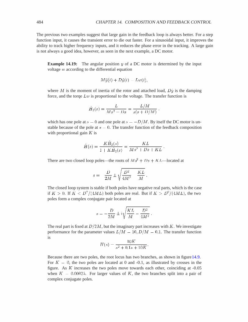
484 CHAPTER 14. COMPOSITION AND FEEDBACK CONTROL
The previous two examples suggest that large gain in the feedback loop is always better. For a stepfunction input, it causes the transient error to die out faster. For a sinusoidal input, it improves theability to track higher frequency inputs, and it reduces the phase error in the tracking. A large gainis not always a good idea, however, as seen in the next example, a DC motor.
Example 14.19: The angular position � of a DC motor is determined by the inputvoltage / according to the differential equation
3 ���� �� ���� � 1/���
where 3 is the moment of inertia of the rotor and attached load, � �� is the dampingforce, and the torqe 1/ is proportional to the voltage. The transfer function is
�;���� �1
3�� ����
1�3
������3��
which has one pole at � � and one pole at � � ���3 . By itself the DC motor is un-stable because of the pole at � � . The transfer function of the feedback compositionwith proportional gain > is
�;��� �> �;����
�> �;�����
>1
3�� ����>1�
There are two closed loop poles—the roots of 3�� ����>1—located at
� � � �
�3"�
��
�3�� >1
3�
The closed loop system is stable if both poles have negative real parts, which is the caseif > 2 . If > ) �����31� both poles are real. But if > 2 �����31�, the twopoles form a complex conjugate pair located at
� � � �
�3" &
�>1
3� ��
�3��
The real part is fixed at ���3 , but the imaginary part increases with > . We investigateperformance for the parameter values 1�3 � � ��3 � �. The transfer functionis
�;��� �>
�� � ��� >�
Because there are two poles, the root locus has two branches, as shown in figure14.9.For > � , the two poles are located at 0 and -0.1, as illustrated by crosses in thefigure. As > increases the two poles move towards each other, coinciding at -0.05when > � ���. For larger values of > , the two branches split into a pair ofcomplex conjugate poles.
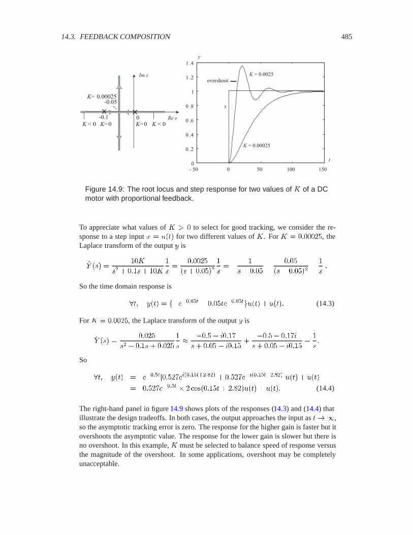
14.3. FEEDBACK COMPOSITION 485
-0.05
-0.1 0K=0
K= 0.00025
K < 0Re s
Im s
K=0K < 0
- 50 0 50 100 1500
0 .2
0 .4
0 .6
0 .8
1
1 .2
1 .4
K = 0.0025
K = 0.00025
t
y
x
overshoot
Figure 14.9: The root locus and step response for two values of > of a DCmotor with proportional feedback.
To appreciate what values of > 2 to select for good tracking, we consider the re-sponse to a step input � � 0�� for two different values of > . For > � ���, theLaplace transform of the output � is
�$ ��� �>
�� � ��� >
��
���
��� ����
�� �
�� ��� ��
��� �����
��
So the time domain response is
�� ��� � ��������� � ���������0�� � 0��� (14.3)
For > � ���, the Laplace transform of the output � is
�$ ��� ����
�� � ��� ���
�� ��� � &��
�� �� � &���
���� ��&
�� �� � &���
��
So
�� ��� � ������������� ����������� � ������� ����������� �0�� � 0��
� ���������� � � ������ � �����0�� � 0��� (14.4)
The right-hand panel in figure 14.9 shows plots of the responses (14.3) and (14.4) thatillustrate the design tradeoffs. In both cases, the output approaches the input as ��,so the asymptotic tracking error is zero. The response for the higher gain is faster but itovershoots the asymptotic value. The response for the lower gain is slower but there isno overshoot. In this example, > must be selected to balance speed of response versusthe magnitude of the overshoot. In some applications, overshoot may be completelyunacceptable.

486 CHAPTER 14. COMPOSITION AND FEEDBACK CONTROL
We can now investigate the proportional feedback control in a general setting. Suppose the planttransfer function is a proper rational polynomial
�;���� �����������
�
where �� has degree 3 , �� has degree � , and 3 � � ( �;� is proper). The closed loop transferfunction is
�;��� �> �;����
�> �;�����
> ���������� �> �����
� (14.5)
The closed loop poles are the � roots of the equation ����� �> ����� � . These roots will dependon > , so we denote them (��>�� � (��>�. As > varies, these roots will trace out the � branchesof the root locus. At > � , the poles are the roots of ����� � , which are the poles of the planttransfer function ������ �����. The stability of the closed loop plant requires that > must be suchthat
Re�(��>� ) � �Re�(��>� ) � (14.6)
Within those values of > that satisfy (14.6) we must select > to get a good response.
The following example shows that a proportional compensator may be unable to guarantee closedloop stability.
Example 14.20: Consider a plant transfer function given by
�;���� ������
������
��
��� ���� � �� �����
There is one zero at � � �, one pole at � � and a pair of complex conjugate polesat � � ��� " &. The plant is unstable because of the pole at � � . The closed looppoles are the roots of the polynomial
� �>� �� � > ����� � ����� � >��� � � ��� ����� ���� � ��
Figure 14.10 shows the three branches of the root locus plot for > 2 . As> increases,the unstable pole moves towards the zero, while the complex conjugate poles move intothe right-half plane. We need to find the values of > that satisfy the stability condition(14.6). The value of > for which the pole at � � moves to � � is obtained fromthe condition � �>� � � , which gives �> � ���� � � � or > � ���. So onecondition for stability is > 2 ���. The complex conjugate poles cross the imaginaryaxis at � � "&���. This occurs at > given by � �>� &���� � which gives > � �.So the second condition for stability is > ) �. The two conditions > 2 ��� and> ) � are inconsistent, so no proportional compensator can stabilize this system.
We return to the general discussion. Suppose the stability condition (14.6) can be met. Among thevalues of > that achieve stability, we select that value for which the output � closely tracks a step
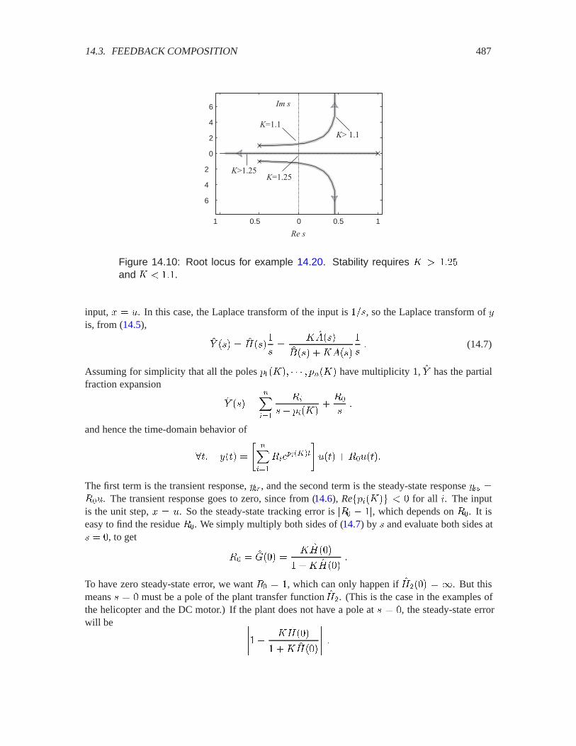
14.3. FEEDBACK COMPOSITION 487
1 0.5 0 0.5 1
6
4
2
0
2
4
6
K=1.25
K=1.1
Re s
Im s
K> 1.1
K>1.25
Figure 14.10: Root locus for example 14.20. Stability requires > 2 ���and > ) �.
input, � � 0. In this case, the Laplace transform of the input is ��, so the Laplace transform of �is, from (14.5),
�$ ��� � �;���
��
> ���������� �> �����
�� (14.7)
Assuming for simplicity that all the poles (��>�� � (��>� have multiplicity 1, �$ has the partialfraction expansion
�$ ��� ���
���
��
�� (��>����
��
and hence the time-domain behavior of
�� ��� �
��
���
���#� ���
�0�� ���0���
The first term is the transient response, ��!, and the second term is the steady-state response ��� ���0. The transient response goes to zero, since from (14.6), Re�(��>� ) for all &. The inputis the unit step, � � 0. So the steady-state tracking error is ��� � �, which depends on ��. It iseasy to find the residue ��. We simply multiply both sides of (14.7) by � and evaluate both sides at� � , to get
�� � �9�� �> �;��
�> �;���
To have zero steady-state error, we want �� � , which can only happen if �;��� � �. But thismeans � � must be a pole of the plant transfer function �;�. (This is the case in the examples ofthe helicopter and the DC motor.) If the plant does not have a pole at � � , the steady-state errorwill be #####� > �;��
�> �;��
##### �

488 CHAPTER 14. COMPOSITION AND FEEDBACK CONTROL
This error is smaller the larger the gain > . So to minimize the steady-state error we should chooseas large a gain as possible, subject to the stability requirement (14.6).
However, a large value of > may lead to poor transient behavior by causing overshoots, as happenedin the DC motor example in figure 14.9 for the larger gain > � ���. To decide the appropriate> is a matter of trial and error. One studies the transient response for different (stabilizing) valuesof > (as we did for the DC motor) and selects > that gives a satisfactory transient behavior.
14.4 PID feedback
The P controller discussed in the previous section achieves zero steady-state error if the plant hasa pole at � � . This means that the plant includes an integrator, since the transfer function of anintegrator is ��, which has a pole at � � . If the plant does not have a pole at � � , however, anon-zero error results. While this error can be reduced by choosing a large gain > in the controller,this results in poor transient behavior.
In this section, we develop the well-known PID controller, which includes an integrator in thecontroller. It can achieve zero steady-state error even if the plant does not have a pole at � � , andstill achieve reasonable transient behavior. The PID controller is a generalization of the P controller,in that with certain choices of parameters, it becomes a P controller.
We begin with an example that has rich enough dynamics to demonstrate the strengths of the PIDcontroller. This example describes a mechanical system, but just about any physical system that ismodeled by a linear second-order differential equation is subject to similar analysis. This includes,for example, electrical circuits having resistors, capcitors, and inductors.
Example 14.21: A basic mass-spring-damper system is illustrated in figure 14.11.This system has a mass 3 that slides on a frictionless surface, a spring that attachesthe mass to a fixed physical object, and a damper, which absorbes mechanical energy.A damper might be, for example, a dashpot, which is a cylinder filled with oil plusa piston. A familiar example of such a damper is a shock absorber in the suspensionsystem of a car.
Suppose that an external force / is applied to the mass, where / is a continuous-timesignal. The differential equation governing the system is obtained by setting the sumof all forces to zero,
3 ���� �� ���� � ���� � /���
The output ��� is the position of the mass at time , 3 ���� is the inertial force, � ����is the damping force due to the damper, ���� is the restoring force of the spring, and/�� is the externally applied force. We assume that ��� � when the spring is in itsequilibrium position (neither extended nor compressed). 3 , �, and � are constants.Taking the Laplace transform, using the differentiation property from table13.4, gives
�� �$ ��� ��� �$ ��� � �$ ��� � 7 ����

14.4. PID FEEDBACK 489
w(t)
D
y(t)
M
C
spring
damper
mass
H2(s) =yw
1Ms2 + Ds + C
Figure 14.11: A mass-spring-damper system.
so the plant or open loop transfer function is
�;���� ��$ ���
�7 ����
3�� ���� ��
Suppose for example that the constants have values 3 � , � � ,and � � ���.Then
�;���� �
�� � �� ���� (14.8)
In this case, the transfer function has a pair of complex poles at � � ��� " &. Sincetheir real part is strictly negative, the system is stable.
Suppose we wish to drive the system to move the mass to the right one unit of distanceat time � . We can apply an input force that is a unit step, scaled so that the steady-state response places the mass at position ��� � . The final steady-state output isdetermined by the DC gain, which is �;�� � ���� � ��, so we can apply an inputgiven by
� � � /�� �
��0�� � ���0���
where 0 is the unit step signal. The resulting response �o has Laplace transform
�$o��� �
�� � �� ��� ���
����� � ���&
�� �� � &����� ���&
�� �� � &�
��
We call this the open-loop step response, because there is no control loop (yet).
Taking the inverse transform gives the open-loop step response
� � �o�� � ����������� � ���&���� � ����� ���&����� �0�� � 0���
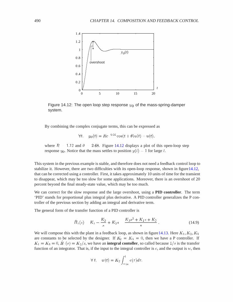
490 CHAPTER 14. COMPOSITION AND FEEDBACK CONTROL
yo(t)
t
overshoot
0 5 10 15 200
0 .2
0 .4
0 .6
0 .8
1
1 .2
1 .4
Figure 14.12: The open loop step response �o of the mass-spring-dampersystem.
By combining the complex conjugate terms, this can be expressed as
�� �o�� � ������� ����� #�0�� � 0���
where � � �� and # � �� �. Figure 14.12 displays a plot of this open-loop stepresponse �o. Notice that the mass settles to position ��� � for large .
This system in the previous example is stable, and therefore does not need a feedback control loop tostabilize it. However, there are two difficulties with its open-loop response, shown in figure14.12,that can be corrected using a controller. First, it takes approximately 10 units of time for the transientto disappear, which may be too slow for some applications. Moreover, there is an overshoot of 20percent beyond the final steady-state value, which may be too much.
We can correct for the slow response and the large overshoot, using a PID controller. The term‘PID’ stands for proportional plus integral plus derivative. A PID controller generalizes the P con-troller of the previous section by adding an integral and derivative term.
The general form of the transfer function of a PID controller is
�;���� � >� �>�
��>�� �
>��� �>���>�
�� (14.9)
We will compose this with the plant in a feedback loop, as shown in figure14.13. Here >��>��>�
are constants to be selected by the designer. If >� � >� � , then we have a P controller. If>� � >� � , �;���� � >���, we have an integral contoller, so called because �� is the transferfunction of an integrator. That is, if the input to the integral controller is �, and the output is /, then
� � /�� � >�
� �
���������

14.4. PID FEEDBACK 491
x e y
H =H1H2
1 + H1 H2
−H2(s) =
w1
Ms2 + Ds + CH1(s) = K1 + K2/s + K3s
PID controller Plant
Figure 14.13: The mass-spring-damper system composed with a PID con-troller in a feedback composition.
If >� � >� � , �;���� � >��, then we have a derivative controller, so called because � is thetransfer function of a differentiator. That is, if the input to the derivative controller is �, and theoutput is /, then
� � /�� � >� �����
The following table offers guidelines for selecting the parameters of a PID controller. Of course,these are guidelines only—the actual performance of the closed loop system depends on the planttransfer function and must be checked in detail.
Parameter Response speed Overshoot Steady-state error>� Faster Larger Decreases>� Faster Larger Zero>� Minor change Smaller Minor change
Example 14.22: We now evaluate a PID controller for the mass-spring-damper systemof figure 14.11, using the feedback composition of figure 14.6. We assume the param-eters values 3 � , � � , and � � ���, as in example 14.21. The closed-looptransfer function with the PID controller is
�;��� ��;���� �;����
� �;���� �;�����
>��� �>���>�
�� � � �>���� � ���� �>����>��
Suppose we provide as input a unit step. This means that we wish to move the massto the right one unit of distance, starting at time � . The controller will attempt totrack this input. The response to a unit step input has Laplace transform
�$#�%��� � �;��� ��
>��� �>���>�
�� � � �>���� � ���� �>����>� �� (14.10)
We now need to select the values for the parameters of the PID controller, >�, >�, and>�. We first try proportional control with >� � , and >� � >� � . In this case,

492 CHAPTER 14. COMPOSITION AND FEEDBACK CONTROL
0 2 4 6 8 10 12 14 16 18 200
0.5
1
1.5
yo
yp
ypd
ypid
Figure 14.14: The step response for open loop, �", with P-control, �#, PD-control, �#%, and PID-control, �pid .
the step response has the Laplace transform
�$#��� �
�� � �� ��� ��
The inverse Laplace transform gives the time response �#, which is plotted in figure14.14. The steady-state value is determined by the DC gain of the closed loop transferfunction,
�� � �� ���
####���
�
���� ����
This yields an error of 11 percent, and the overshoot of 50 percent is much worse thanthat of the open-loop response �", also shown in the figure. Thus, a P controller withgain > � is useless for this application.
Following the guidelines in the table above, we add derivative control to reduce theovershoot. The result is a so-called PD controller, because it adds a proportional and aderivative term. For the PD controller we choose >� � and >� � . Substitution
14.5. SUMMARY 493
in (14.10) gives the Laplace transform of the step response,
�$#%��� ���
�� � �� ��� ��
The steady-state value is given by the DC gain of the closed loop transfer function,
��
�� � �� ���
####���
� ����
which is the same as the steady-state value for the P controller. The inverse Laplacetransform gives the time response �pd, which is plotted in figure 14.14. The overshootis reduced to 10 percent—a large improvement. Also, the response is quicker—thetransient disappears in about 4 time units.
Finally, to eliminate the steady-state error we add integral control. For the PID con-troller we choose >� � �>� � ��>� � . Substitution in (14.10) gives theLaplace transform of the step response
�$pid��� ��� � �� �
�� � �� � ���� � � ��
The steady-state value is again given by the DC gain of the closed loop transfer func-tion,
�� � �� �
�� � �� � ���� � �
#####���
� �
So the steady-state error is eliminated, as expected. The time response �pid is plottedin figure 14.14. It shows significant improvement over the other responses. There isno overshoot, and the transient disappears in about 4 time units. Further tuning of theparameters >��>��>� could yield small improvements.
14.5 Summary
This chapter considers cascade, parallel, and feedback compositions of LTI systems described byZ or Laplace transforms. Cascade composition is applied to equalization, parallel composition isapplied to noise cancellation, and feedback composition is applied to control.
Because we are using Z and Laplace transforms rather than Fourier transforms, we are able to con-sider unstable systems. In particular, we find that while, in principle, cascade and parallel composi-tions can be used to stabilize unstable systems, the result is not robust. Small changes in parametervalues can result in the system being once again unstable. Feedback composition, on the other hand,can be used to robustly stabilize unstable systems. We illustrate this first with a simple helicopterexample. The second example, a DC motor, benefits from more sophisticated controllers. Thethird example, a mass-spring-damper system, motivates the development of the well-known PIDcontroller structure. PID controllers can be used to stabilize unstable systems and to improve theresponse time, precision, and overshoot of stable systems.
494 CHAPTER 14. COMPOSITION AND FEEDBACK CONTROL
Exercises
Each problem is annotated with the letter E, T, C which stands for exercise, requires some thought,requires some conceptualization. Problems labeled E are usually mechanical, those labeled T re-quire a plan of attack, those labeled C usually have more than one defensible answer.
1. E This exercise studies equalization when the channel is only known approximately. Considerthe cascade composition of figure 14.1, where �;� is the channel to be equalized, and �;� isthe equalizer. If the equalizer is working perfectly, then � � �. For example, if
�;���� ��
� � ��and �;���� �
� � ��
��
then � � � because �;���� �;���� � .
(a) Suppose that �;���� is as given above, but the plant is a bit different,
�;���� ��
� � ��� A�
Suppose that � � Æ, the Kronecker delta function. Plot �� � for A � � and A � ��.
(b) Now suppose that the equalizer is
�;���� �� � �
��
and the channel is�;���� �
�
� � �� A�
Again suppose that � � Æ, the Kronecker delta function. Plot � � � for A � ����.
(c) For part (b), show that equalization error � � � grows without bound whenever A �� ,�A� ) .
2. E This exercise studies equalization for continuous-time channels. Consider the cascade com-position of figure 14.1, where �;� is the channel to be equalized, and �;� is the equalizer. Bothare causal. If
�;���� ���
�� �and �;���� �
�� �
�� �
then � � � because �;���� �;���� � .
(a) Suppose �;� is as above but
�;���� ���
�� � � A�
Suppose � � 0, the unit step. Plot � � � for A � � and A � ��, and calculate thesteady state error.
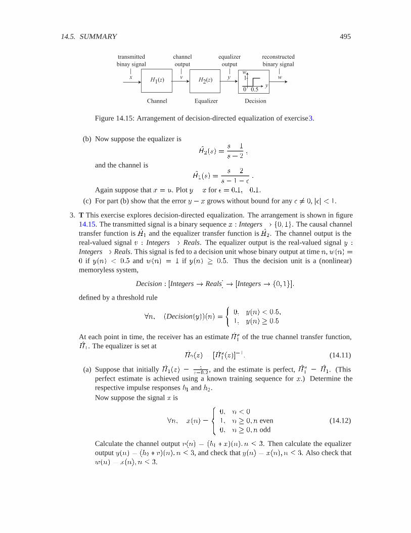
14.5. SUMMARY 495
x v y wy
w
0.50
1H1(z) H2(z)
Channel Equalizer Decision
transmittedbinay signal
equalizeroutput
reconstructedbinary signal
channeloutput
Figure 14.15: Arrangement of decision-directed equalization of exercise3.
(b) Now suppose the equalizer is�;���� �
��
�� ��
and the channel is�;���� �
�� �
�� � A�
Again suppose that � � 0. Plot � � � for A � �����(c) For part (b) show that the error � � � grows without bound for any A �� , �A� ) .
3. T This exercise explores decision-directed equalization. The arrangement is shown in figure14.15. The transmitted signal is a binary sequence � � Integers� �� . The causal channeltransfer function is �;� and the equalizer transfer function is �;�. The channel output is thereal-valued signal " � Integers� Reals. The equalizer output is the real-valued signal � �Integers� Reals. This signal is fed to a decision unit whose binary output at time �, /��� � if ���� ) �� and /��� � if ���� � ��. Thus the decision unit is a (nonlinear)memoryless system,
Decision� �Integers� Reals�� �Integers� �� ��defined by a threshold rule
��� �Decision������� �
�� ���� ) ���� ���� � ��
At each point in time, the receiver has an estimate �; � of the true channel transfer function,
�;�. The equalizer is set at�;���� � � �;
�������� (14.11)
(a) Suppose that initially �;���� � ������ , and the estimate is perfect, �;
� � �;�. (Thisperfect estimate is achieved using a known training sequence for �.) Determine therespective impulse responses �� and ��.Now suppose the signal � is
��� ���� �
����
� � ) � � � � � even� � � � � odd
(14.12)
Calculate the channel output "��� � ��� � ������ � � �. Then calculate the equalizeroutput ���� � ��� � "����� � � �, and check that ���� � ����� � � �. Also check that/��� � ����� � � �.

496 CHAPTER 14. COMPOSITION AND FEEDBACK CONTROL
(b) Now suppose the channel transfer function has changed to
�;���� ��
� � ���
but the receiver’s estimate hasn’t changed, i.e.
�; ���� �
�
� � ���
so the equalizer (14.11) hasn’t change either. For the same input signal again calculatethe channel and equalizer outputs "���� ����� � � �. Check that ���� �� ����� � 2 .But show that the decision /��� � ����� � � �. So the equalizer correctly determines�.
(c) Since the receiver’s decision / � �, it can make a new estimate of the channel usingthe fact that �$ � �;�
�;��� � �;�
�;��7 . The new estimate is
�; � �
�$
�;��7� (14.13)
Suppose time is �, and the receiver has observed ����� /���� � � �. Since the Z trans-forms �$ and �7 also depend on values of ����� /��� for � 2 �, these Z transformscan not be calculated at time � � �, and so the estimator (14.13) cannot be used. Thefollowing approach will work, however.
Suppose the receiver knows that the unknown channel transfer function is of the form
�;���� ��
� � ��
so that only the parameter � has to be estimated. Using this information, we have
�$ ��� ��
� � �
� � ��
��7 ��� �
� � ��
� � �7 ����
Now take the inverse Z transform and express the time-domain relation between � and/. Show that you can estimate � knowing ���� ���� /��� /��.
4. E This continues exercise 3. It shows that if the channel estimate �; � is not sufficiently close
to the true channel �;�, the decision may become incorrect. Suppose the true channel is�;���� �
���� , the estimate is �;
���� ��
����� , the equalizer is �;���� � � �; �����
�� � ������ ,
and the decision is as in figure 14.15. Assume the input signal � to be the same as in (14.12)Show that if � � � then /�� � ���� /�� � ���� /��� � ����, but /��� �� ����.
5. E This exercise continues the discussion in examples 14.5, 14.6 for the continuous-time,causal and stable channel with impulse response �� and transfer function
�� RoC���� � �� � Re�� 2 �� �;���� ��� �
�� �
(a) Calculate �� and sketch it. (Observe how the zero in the right-half plane at � � �accounts for the negative values.)
14.5. SUMMARY 497
(b) The inverse of �;�,�;���� �
��
�� ��
has a pole at � � �. So as a causal system, the inverse is unstable. But as a non-causalsystem, it is stable with RoC � �� � Re�� ) � which includes the imaginary axis.Evaluate the impulse response �� of �;� as an anti-causal system, and give a sketch.
(c) The impulse response �� calculated in (a) is non-zero for � . Consider the finite-duration, anti-causal impulse response �� obtained by truncating �� before time -5,
� Reals� ���� �
������ � ��� ) ��
and sketch ��. Calculate the transfer function �;�, including its RoC, by using thedefinition of the Laplace transform.
(d) Obtain the causal impulse response � by delaying �� by time , i.e.
� Reals� ��� � ���� ��
Sketch � and find its transfer function, �;. Then �; is an approximate inverse of �;�
with a delay of 5 time units. (Note: �� has a delta function at 0.)
6. T The proportional controller of figure 14.7 stabilizes the plant for > 2 . In this exercise,we try to achieve the same effect by the cascade compensator of figure14.1.
(a) Assume that the plant �;� is as given in figure 14.7. Design �;� for the cascade com-position of figure 14.1 so that �;�
�;� is the same as the closed-loop transfer functionachieved in figure 14.7.
(b) Now suppose that the model of the plant is not perfect, and the plant’s real transferfunction is
�;���� �
3��� A��
for some small value of A 2 . Using the same �;� that you designed in part (a), what isthe transfer function of the cascade composition? Is it stable?
7. T Consider a discrete-time causal plant with transfer function
�;���� ��
� � ��
(a) Where are the poles and zeros? Is the plant stable?
(b) Find the impulse response of the plant. Is it bounded?
(c) Give the closed-loop transfer function for the P controller for this plant.
(d) Sketch the root locus for the P controller for this plant.
(e) For what values of > is the closed-loop system stable?
(f) Find the step response of the closed-loop system. Identify the transient and steady-stateresponses. For > � , what is the steady-state tracking error?
498 CHAPTER 14. COMPOSITION AND FEEDBACK CONTROL
(g) Suppose that the plant is instead given by
�;� ��
� � �� A�
for some real A � . For what values of > is the P controller robust for plants with�A� ) ��?
8. T Consider the feedback composition in figure14.6. Suppose that �;��;� is causal and strictly
proper, meaning that the order of the numerator is greater than the order of the denominator.
(a) Show that if �;��;� is causal and strictly proper, then so is �;, the transfer function of
the feedback composition given by (14.1).
(b) For the discrete-time case, show that we can write
�;���� �;���� � ��� �9���� (14.14)
where 9��� is proper, and is the transfer function of a causal system. Intuitively, thismeans that there must be a net unit delay in the feedback loop, because ��� is thetransfer function of a unit delay.
(c) Use the result of part (a) to argue that the system �;��;� has state-determined output.
(d) For the continuous-time case, show that we can write
�;���� �;���� � ��� �9���� (14.15)
where 9��� is proper, and is the transfer function of a causal system. Intuitively, thismeans that there must be an integration in the feedback loop, because ��� is the transferfunction of an integrator.
(e) Use the result of part (c) to argue that the system �;��;� has state-determined output,
assuming that the input is bounded and piecewise continuous.
Appendix A
Sets and Functions
This appendix establishes the notation of sets and functions as used in the book. We review theuse of this mathematical language to describe sets in a variety of ways, to combine sets using theoperations of union, intersection, and product, and to derive logical consequences. We also reviewhow to formulate and understand predicates, and we define certain sets that occur frequently in thestudy of signals and systems. Finally, we review functions.
A.1 Sets
A set is a collection of elements. The set of natural numbers, for example, is the collection of allpositive integers. This set is denoted (identified) by the name Naturals,
Naturals� �� �� �� � (A.1)
In (A.1) the left hand side is the name of the set and the right hand side is an enumeration or list ofall the elements of the set. We read (A.1) as ‘Naturals is the set consisting of the numbers � �� ��and so on.’ The ellipsis ‘ ’ means ‘and so on’. Because Naturals is an infinite set we cannotenumerate all its elements, and so we have to use ellipsis. For a finite set, too, we may use ellipsisas a convenient shorthand as in
� � �� �� �� � � (A.2)
which defines � to be the set consisting of the first 100 natural numbers. Naturalsand � are sets ofnumbers. The concept of sets is very general, as the examples below illustrate.
Studentsis the set of all students in this class, each element of which is referenced by a student’sname:
Students� �John Brown� Jane Doe� Jie Xin Zhou� �USCitiesconsists of all cities in the U.S., referenced by name:
USCities� �Albuquerque�San Francisco�New York� �
499
500 APPENDIX A. SETS AND FUNCTIONS
BooksInLibcomprises all books in the U.C. Berkeley library, referenced by a 4-tuple (first author’slast name, book title, publisher, year of publication):
BooksInLib � �(Lee, Digital Communication, Kluwer, 1994)�
(Walrand, Communication Networks, MorganKaufmann, 1996)� �BookFilesconsists of all LATEX documents for this book, referenced by their file name:
BookFiles� �sets.tex� functions.tex� �We usually use either italicized, capitalized names for sets, such as Realsand Integers, or singlecapital letters, such as ������ $ .
An element of a set is also said to be a member of the set. The number is a member of the set �defined in (A.2), but the number is not a member of �. We express these two facts by the twoexpressions:
�� � ��
The symbol ‘’ is read ‘is a member of’ or ‘belongs to’ and the symbol ‘�’ is read ‘is not a memberof’ or ‘does not belong to.’
When we define a set by enumerating or listing all its elements, we enclose the list in curly braces� . It is not always necessary to give the set a name. We can instead refer to it directly byenumerating its elements. Thus
�� �� �� �� �is the set consisting of the numbers � �� � �.
The order in which the elements of the set appear in the list is not (usually) significant. When theorder is significant, the set is called an ordered set.
An element is either a member of a set or it is not. It cannot be a member more than once. So, forexample, �� �� is not a set.
Thus a set is defined by an unordered collection of its elements, without repetition. Two sets areequal if and only if every element of the first set is also an element of the second set, and every ele-ment of the second set is a member of the first set. So if � � �� �� �� �� � and � � ��� �� �� � �,then it is correct to state
� � �� (A.3)
A.1.1 Assignment and assertion
Although the expressions (A.1) and (A.3) are both in the form of equations, the “=” in these twoexpressions have very different meanings. Expression (A.1) (as well as (A.2)) is an assignment:the set on the right-hand side is assigned to the name Naturalson the left-hand side. Expression(A.3) is an assertion, which is an expression that can be true or false. In other words, an assertionis an expression that has a truth value. Thus (A.3) asserts that the two sides are equal. Since this istrue, (A.3) is a true assertion. But the assertion
Naturals� �

A.1. SETS 501
is a false assertion. An assertion is true or false, while an assignment is a tautology (somethingthat is trivially true because the definition makes it so). Some notation systems make a distinctionbetween an assignment and an assertion by writing an assignment using the symbol “:=” instead of“=” as in
Naturals �� �� �� �� �Other notation systems use “=” for assignments and ‘==’ for assertions. We will not make thesenotational distinctions (except in chapter 6), since it will be clear from the context whether anexpression is an assignment or an assertion.1
Context is essential in order to disambiguate whether an expression like “MyNumbers� �� �� �”is an assertion or an assignment. Thus, for example, in the context,
Define the set MyNumbersby MyNumbers� �� �� ��the expression is clearly an assignment, as indicated by “Define the set ”. However, in thefollowing context,
If we define MyNumbersby MyNumbers� �� �� �� then MyNumbers� ��� �� �
the first “=” is an assignment, but the second is an assertion.
A.1.2 Sets of sets
Anything can be an element of a set, so of course, sets can be elements of sets. Suppose, forexample, that � is a set. Then we can construct the set of all subsets of � , which is written � ���and is called the power set of � .2 Notice that since � � � , then � � ���. (� denotes the emptyset.)
A.1.3 Variables and predicates
We can refer to a particular element of a set by using its name, for example the element �� inNaturals, or Berkeley in USCities. We often need to refer to a general element in a set. We do thisby using a variable. We usually use lower case letters for variable names, such as �� �� �� . Thus� Naturalsrefers to any natural number. Naturals is the range of the variable �. We may alsouse a character string for a variable name such as city USCities. We say that “� is a variable overNaturals” and “city is a variable over USCities.”.
A variable can be assigned (or substituted by) any value in its range. Thus the assignment � � �assigns the value � to �, and city � Berkeley assigns the value Berkeley to city.
Once again the use of “=” in an expression like � � � is ambiguous, because the expression couldbe an assignment or an assertion, depending on the context. Thus, for example, in the context,
1A symbol such as “=” which has more than one meaning depending on the context is said to be overloaded. C++ usesoverloaded symbols, while Java does not (Java does support overloaded methods, however). People often have difficultyreading other people’s code written in a language that permits overloading.
2The power set of � is sometimes written �� .
502 APPENDIX A. SETS AND FUNCTIONS
Probing further: Predicates in Matlab
In Matlab, “=” is always used as an assignment, while “==” is used to express anassertion. Thus the Matlab program,
n = 5, m = 6, k = 2, m = k+n
returns
n = 5, m = 6, k = 2, m =7
because the expression m=k+n assigns the value 7 to m. However, the Matlabprogram
n = 5, m = 6, k = 2, m == k+n
returns
n = 5, m = 6, k = 2, ans = 0
where ans = 0 means that the assertion m == k+n evaluates to false.
Let � � ��' � � 6 � �, then ' � 6 � �
the first three “=” are assignments, but the last is an assertion, which happens to be false.
We can use variables to form expressions such as � � �. Now, when we assign a particular value to� in this expression, the expression become an assertion that evaluates to true or false. (For instance,� � � evaluates to true for � � � and to false for � � .) An expression such as � � � whichevaluates to true or false when we assign the variable a specific value is called a predicate (in �).3
Predicates are used to define new sets from old ones, as in this example:
� � �� Naturals� � � �
which reads “� is the set of all elements � in Naturalssuch that (the symbol ‘�’ means ‘such that’)the predicate � � � is true.” More generally, we use the following prototype expression to define anew set NewSetfrom an old set Set
NewSet� �� .� � Pred���� (A.4)
3A specific value is said to satisfy a predicate if it evaluates to true, and not to satisfy the predicate if the predicateevaluates to false.

A.1. SETS 503
In this prototype expression for defining sets, � Setmeans that � is a variable over the set Set,Pred��� is a predicate in �, and so NewSetis the set consisting of all elements � in Setfor whichPred��� evaluates to true.
We illustrate the use of the prototype (A.4). In the examples below, note that the concept of predicateis very general. In essence, a predicate is a condition involving any attributes or properties of theelements of Set. Consider
TallStudents� �name Students� nameis more than 6 feet tall�Here the predicate is “nameis more than 6 feet tall.” If John Brown’s height is 5’ 10” and JaneDoe is 6’1” tall, the predicate evaluates to true for name= Jane Doe, and to false for name= JohnBrown, so Jane Doe TallStudentsand John Brown � TallStudents. Consider
NorthCities� �city USCities� city is located north of Washington DC�The predicate here evaluates to true for city = New York, and to false for city = Atlanta.
The variable name “�” used in (A.4) is not significant. The sets �� Naturals � � � � and�� Naturals� � � � are the samesets even though the variable names used in the predicates aredifferent. This is because the predicates ‘� � �’ and ‘� � �’ both evaluate to true or both evaluateto false when the same value is assigned to � and �. We say that the variable name � used in (A.4) isa dummy variable since the meaning of the expression is unchanged if we substitute � with anothervariable name, say �. You are already familiar with the use of dummy variables in integrals. Thetwo integrals below evaluate to the same number:� �
����� �
� �
������
A.1.4 Quantification over sets
Consider the set � � �� �� �. Suppose we want to make the assertion that every element of � issmaller than 7. We could do this by the three expressions
) �� � ) �� � ) ��
which gets to be very clumsy if � has many more elements. So mathematicians have invented ashorthand. The idea is to be able to say that � ) � for every value that the variable � takes in the set�. The precise expression is
�� �� � ) �� (A.5)
The symbol ‘�’ reads ‘for all’, so the expression reads, “for all values of � in �, � ) �.” The phrase�� � is called universal quantification. Note that in the expression (A.5), � is again a dummyvariable; the meaning of the expression is unchanged if we use another variable name. Note, also,that (A.5) is an assertion which, in this case, evaluates to true. However, the assertion
�� �� � 2 �
is false, since for at least one value of � �, namely � � , � 2 � is false.
504 APPENDIX A. SETS AND FUNCTIONS
Suppose we want to say that there is at least one element in � that is larger than 3. We can say thisusing existential quantification as in
�� �� � 2 �� (A.6)
The symbol ‘�’ reads ‘there exists’, so the expression (A.6) reads ‘there exists a value of � in �,� 2 �’. Once again, any other variable name could be used in place of �, and the meaning of theassertion is unchanged.
In general, the expression,�� �� Pred���� (A.7)
is an assertion that evaluates to true if Pred��� evaluates to true for every value of � �, and
�� �� Pred���� (A.8)
is an assertion that evaluates to true if Pred��� evaluates to true for at least one value of � �.
Conversely, the assertion (A.7) evaluates to false if Pred��� evaluates to false for at least one valueof � �, and the assertion (A.8) evaluates to false if Pred��� evaluates to false for every value of� �.
We can use these two quantifiers to define sets using the prototype new set constructor (A.4). Forexample
EvenNumbers� �� Naturals� �6 Naturals� � � �6is the set of all even numbers, since the predicate in the variable �,
�6 Naturals� � � �6�
evaluates to true if and only if � is even.
A.1.5 Some useful sets
The following sets are frequently used in the book:
Naturals� �� �� natural numbersNaturals� � �� � �� non-negative integers
Integers� � ������ � � �� integersIntegers� � �� � �� non-negative integers, same as Naturals�
Reals� ������ real numbersReals� � ���� non-negative real numbers
Complex� ��� � � �� � Reals complex numbers, ���
If *� + are real numbers, then
�*� +� � �� Reals� * � � � +�*� +� � �� Reals� * ) � ) +�*� +� � �� Reals� * ) � � +
������ � Reals
A.1. SETS 505
Note the meaning of the difference in notation: both end-points * and + are included in �*� +�,and we say that �*� +� is a closed interval; neither end-point is included in �*� +�, and we call thisan open interval; the interval �*� +� is said to be half-open, half-closed. Whether an end-point isincluded in an interval or not is indicated by the use of square brackets �� � or parentheses �� �.
Other useful sets are:
Binary� �� � the binary valuesBinary� � �� �� set of all finite binary strings
Bools� �true� false� truth valuesBools� � �true� false�� set of all finite sequences of truth values
Char � set of all alphanumeric charactersChar� � set of all finite character strings
A.1.6 Set operations: union, intersection, complement
Let � � �� �� � , and � � �� � �. Clearly � is included in �, and � is included inNaturals. We express these assertions as:
� � �� � � Naturals�
which we read “� is contained in or included in �” and “� is contained in or included in Naturals.”For the sets above,
Naturals� Naturals� � Integers� Reals� Complex�
If � and � are sets, then � � � is the set consisting of all elements that are in both � and �, and� � � is the set consisting of all elements that are either in � or in � or in both � and �. � � �is called the intersection of � and �, and � � � is called the union of � and �. We can expressthese definitions using variables as:
� �� � �� � � � � � �� � �� � �� � � � � � �
where � is the notation for the logical and and � is the symbol for the logical or. The predicate“� � � � �” reads “� is a member of � and � is a member of �”; “� � � � �” reads“� is a member of � or � is a member of �.” The logical and of two predicates is also called theirconjunction and their logical or is also called their disjunction. The symbols � and � are calledlogical connectives.
If ��� are sets, then � # � is the set consisting of all elements in � that are not in � (think of itas set subtraction, � ��). When � � � , � #� is called the complement of � in � . When � isunderstood, we can write �� instead of � #�.
We gain some intuitive understanding by depicting sets and set operations using pictures. FigureA.1 illustrates union, intersection, and complement.
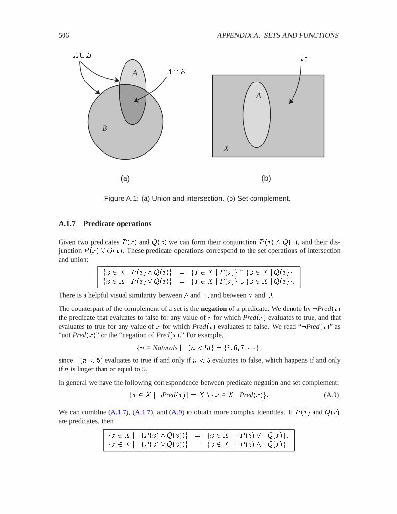
506 APPENDIX A. SETS AND FUNCTIONS
A
B
A
X
(a) (b)
� ��
� ����
Figure A.1: (a) Union and intersection. (b) Set complement.
A.1.7 Predicate operations
Given two predicates � ��� and G��� we can form their conjunction � ��� � G���, and their dis-junction � ��� � G���. These predicate operations correspond to the set operations of intersectionand union:
�� � � � ��� �G��� � �� � � � ��� � �� � � G����� � � � ��� �G��� � �� � � � ��� � �� � � G����
There is a helpful visual similarity between � and �, and between � and �.
The counterpart of the complement of a set is the negation of a predicate. We denote by �Pred���the predicate that evaluates to false for any value of � for which Pred��� evaluates to true, and thatevaluates to true for any value of � for which Pred��� evaluates to false. We read “�Pred���” as“not Pred���” or the “negation of Pred���.” For example,
�� Naturals� ��� ) �� � ��� � �� �since ��� ) �� evaluates to true if and only if � ) � evaluates to false, which happens if and onlyif � is larger than or equal to 5.
In general we have the following correspondence between predicate negation and set complement:
�� � � �Pred��� � � # �� � � Pred���� (A.9)
We can combine (A.1.7), (A.1.7), and (A.9) to obtain more complex identities. If � ��� and G���are predicates, then
�� � � ��� ��� �G���� � �� � � �� ��� � �G������ � � ��� ��� �G���� � �� � � �� ��� � �G����

A.1. SETS 507
These identities have counterparts for set operations. For some set � , if and $ � � and % � � ,then
� # �$ � %� � �� # $ � � �� # %��� # �$ � %� � �� # $ � � �� # %��
When the set � is understood, we can write these as
�$ � %�� � $ � � %���$ � %�� � $ � � %��
These identities are called de Morgan’s rules.
A.1.8 Permutations and combinations
Given a set � with a finite number � of elements, we sometimes wish to construct a subset with afixed number ' � � of elements. The number of such subsets is given by�
�
'
��
��
'����'��� (A.10)
where the exclamation point denotes the factorial function. The notation,��
-is read “� choose '”.
It gives the number of combinations of ' elements from the set �.
A combination is a set, so order does not matter. Sometimes, however, order matters. Suppose forexample that � � ��� �� !. The number of subsets with two elements is�
�
�
��
��
����
�� ��
These subsets are ��� �, ��� !, and ��� !. Suppose instead that we wish to construct orderedsubsets of � with two elements. In other words, we wish to consider ��� �� to be distinct from ��� ��(note the temporary use of square brackets to avoid confusion with unordered sets). Such orderedsubsets are called permutations. The number of '-element permutations of a set of size � is givenby
��
���'��� (A.11)
The number of permutations is a factor of '� larger than the number of combinations inA.10. Forexample, the number of 2-element permutations of � � ��� �� ! is six. They are ��� ��, ��� !�, ��� !�,��� ��, �!� ��, and �!� ��.
A.1.9 Product sets
The product � � $ of two sets � and $ consists of all pairs of elements ��� �� with � � and� $ , i.e.
� � $ � ���� �� � � �� � $ �
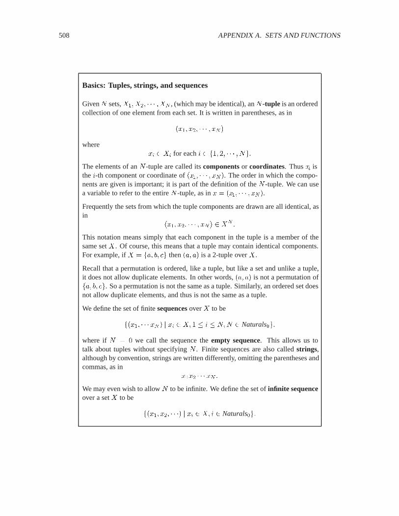
508 APPENDIX A. SETS AND FUNCTIONS
Basics: Tuples, strings, and sequences
Given � sets, ������ ��� , (which may be identical), an � -tuple is an orderedcollection of one element from each set. It is written in parentheses, as in
���� ��� � �� �
where�� �� for each & �� �� � ��
The elements of an � -tuple are called its components or coordinates. Thus �� isthe &-th component or coordinate of ���� � �� �. The order in which the compo-nents are given is important; it is part of the definition of the � -tuple. We can usea variable to refer to the entire � -tuple, as in � � ���� � �� �.
Frequently the sets from which the tuple components are drawn are all identical, asin
���� ��� � �� � �� �
This notation means simply that each component in the tuple is a member of thesame set � . Of course, this means that a tuple may contain identical components.For example, if � � ��� �� ! then ��� �� is a 2-tuple over � .
Recall that a permutation is ordered, like a tuple, but like a set and unlike a tuple,it does not allow duplicate elements. In other words, ��� �� is not a permutation of��� �� !. So a permutation is not the same as a tuple. Similarly, an ordered set doesnot allow duplicate elements, and thus is not the same as a tuple.
We define the set of finite sequences over � to be
����� �� � � �� �� � & � ��� Naturals��
where if � � we call the sequence the empty sequence. This allows us totalk about tuples without specifying � . Finite sequences are also called strings,although by convention, strings are written differently, omitting the parentheses andcommas, as in
���� �� �We may even wish to allow � to be infinite. We define the set of infinite sequenceover a set � to be
����� ��� � � �� �� & Naturals��
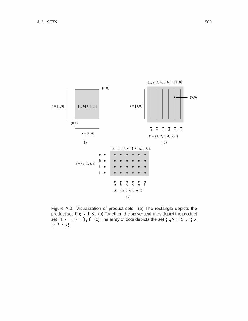
A.1. SETS 509
(0,1)
(6,8)
(5,6)
X = [0,6]
(a) (b)
X = {1, 2, 3, 4, 5, 6}
Y = [1,8] [0, 6] × [1,8]
(c)
a b c d e f
g
h
i
j
X = {a, b, c, d, e, f}
Y = {g, h, i, j}
{a, b, c, d, e, f} × {g, h, i, j}
Y = [1,8]
1 2 3 4 5 6
{1, 2, 3, 4, 5, 6} × [1, 8]
Figure A.2: Visualization of product sets. (a) The rectangle depicts theproduct set �� ���� ��. (b) Together, the six vertical lines depict the productset �� � � �� ��. (c) The array of dots depicts the set ��� �� !� �� �� � ���� �� &� .

510 APPENDIX A. SETS AND FUNCTIONS
The product of two sets may be visualized as in figure A.2. These pictures are informal, to beused only to reinforce intuition. In figure A.2(a), the set � � �� � is represented by a horizontalline segment, and the set $ � �� �� is represented by the vertical line segment. The product set� �$ � �� �� �� �� is represented by the rectangle whose lower left corner is the pair �� � andupper right corner is � � ��.
In figure A.2(b), the discrete set � � �� �� �� �� �� is represented by six points, while and $ ��� �� is represented the same as before. The product set is depicted by six vertical line segments, onefor each element of � . For example, the fifth segment from the left is the set ���� �� � � � � �.One point in that set is shown.
In figure A.2(c), the product of two discrete sets is shown as an array of points. Unless these areordered sets, there is no significance to the the left-to-right or top-to-bottom order in which thepoints are shown. In all three cases in the figure, there is no significance to the choice to depict thefirst set in the product � � $ on the horizontal axis, and the second set on the vertical axis. Wecould have done it the other way around. Although there is no significance to which is depicted onthe vertical axis and which on the horizontal, there is significance to the order of � and $ in ��$ .The set � � $ is not the same as $ �� unless � � $ .
We generalize the product notation to three or more sets. Thus if ��$�% are sets, then � � $ �%is the set of all triples or 3-tuples,
� � $ � % � ���� �� �� � � �� � $� � %�
and if there are � sets, ������ ��� , their product is the set consisting of � -tuples,
�� � ��� � ����� � �� � � �� ��� & � � � �� (A.12)
We can alternatively write (A.12) as
�.���
��� (A.13)
The large ' operator indicates a product of its arguments.
� � � is also written as ��. The � -fold product of the same set � is also written as �� . Forexample, Reals� is the set of all � -tuples of real numbers, and Complex� is the set of all � -tuplesof complex numbers. In symbols,
Reals� � �� � ���� � �� � � �� Reals� & � � � ��Complex� � �� � ���� � �� � � �� Complex� & � � � ��
Predicates on product sets
A variable over ��$ is denoted by a pair ��� ��, with � as the variable over � and � as the variableover $ . We can use predicates in � and � to define subsets of � � $ .
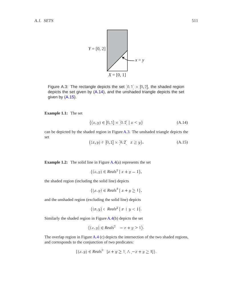
A.1. SETS 511
x = y
Y = [0, 2]
X = [0, 1]
Figure A.3: The rectangle depicts the set �� � � �� ��, the shaded regiondepicts the set given by (A.14), and the unshaded triangle depicts the setgiven by (A.15).
Example 1.1: The set
���� �� �� � � �� �� � � � � (A.14)
can be depicted by the shaded region in FigureA.3. The unshaded triangle depicts theset
���� �� �� � � �� �� � � � �� (A.15)
Example 1.2: The solid line in Figure A.4(a) represents the set
���� �� Reals� � �� � � �
the shaded region (including the solid line) depicts
���� �� Reals� � �� � � �
and the unshaded region (excluding the solid line) depicts
���� �� Reals� � �� � ) �
Similarly the shaded region in Figure A.4(b) depicts the set
���� �� Reals� � � �� � � �
The overlap region in Figure A.4 (c) depicts the intersection of the two shaded regions,and corresponds to the conjunction of two predicates:
���� �� Reals� � ��� � � � � ���� � � ��

512 APPENDIX A. SETS AND FUNCTIONS
(a)
-x + y = 1
(b)
x + y = 1
(c)
x + y = 1-x + y = 1
Figure A.4: (a) The solid line depicts the subset of Reals� satisfying thepredicate � � � � . The shaded region satisfies � � � � . (b) The solidline satisfies �� � � � , and the shaded region satisfies �� � � � . (c)The overlap region satisfies ��� � � � � ���� � � �.
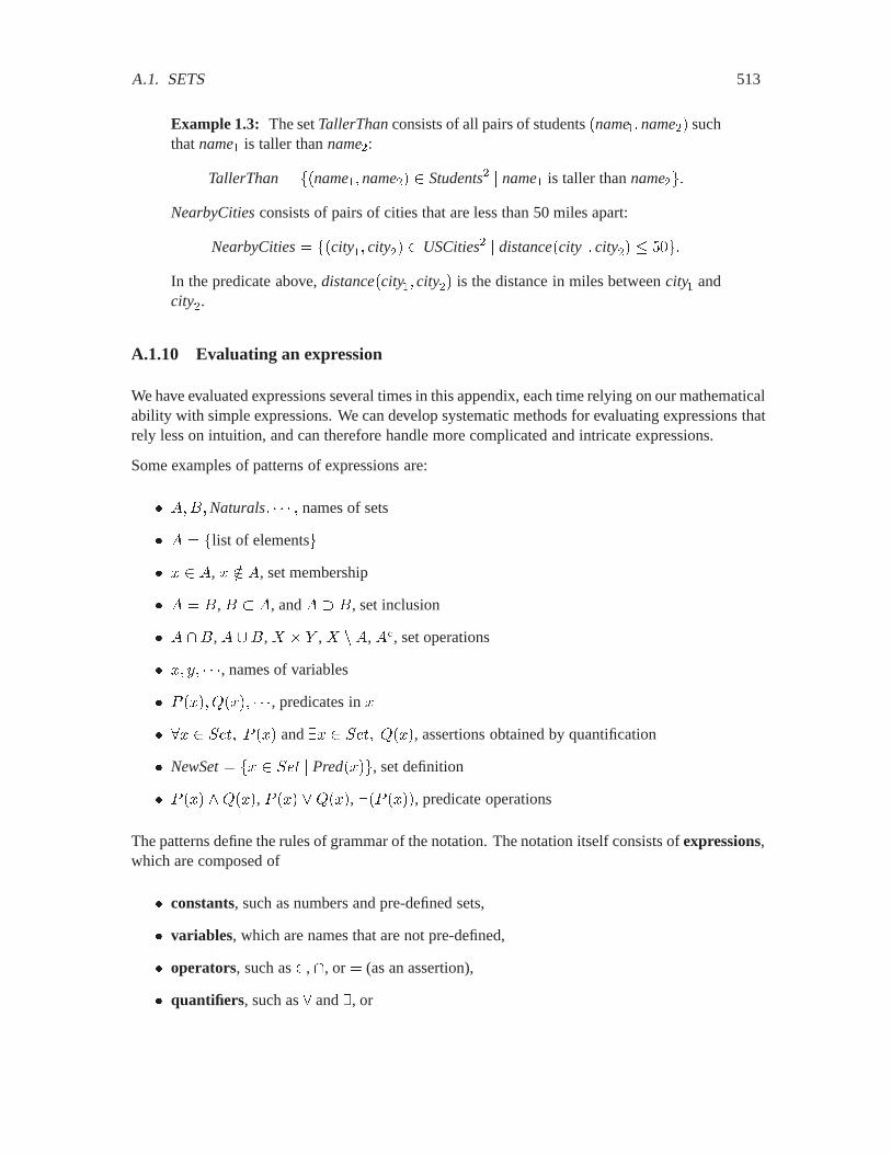
A.1. SETS 513
Example 1.3: The set TallerThanconsists of all pairs of students �name��name�� suchthat name� is taller than name�:
TallerThan� ��name��name�� Students� � name� is taller than name��NearbyCitiesconsists of pairs of cities that are less than 50 miles apart:
NearbyCities� ��city�� city�� USCities� � distance�city�� city�� � ��
In the predicate above, distance�city�� city�� is the distance in miles between city� andcity�.
A.1.10 Evaluating an expression
We have evaluated expressions several times in this appendix, each time relying on our mathematicalability with simple expressions. We can develop systematic methods for evaluating expressions thatrely less on intuition, and can therefore handle more complicated and intricate expressions.
Some examples of patterns of expressions are:
� ����Naturals� � names of sets
� � � �list of elements� � �, � � �, set membership
� � � �, � � �, and � �, set inclusion
� � ��, � ��, � � $ , � # �, ��, set operations
� �� �� , names of variables
� � ���� G���� , predicates in �
� �� .�� � ��� and �� .�� G���, assertions obtained by quantification
� NewSet� �� .� � Pred���, set definition
� � ��� �G���, � ��� �G���, ��� ����, predicate operations
The patterns define the rules of grammar of the notation. The notation itself consists of expressions,which are composed of
� constants, such as numbers and pre-defined sets,
� variables, which are names that are not pre-defined,
� operators, such as , �, or � (as an assertion),
� quantifiers, such as � and �, or

514 APPENDIX A. SETS AND FUNCTIONS
� definitions, namely � (as an assignment).
An expression is well-formed if it conforms to the established patterns.4 For example, if ��G and� are predicates, then the syntax implies that
������ ���� �G���� � �� ��� � ����� � ��� ������� (A.16)
is also a predicate. Just as in the case of a computer language, you learn the syntax of mathematicalexpressions through practice.5
In an expression, constants have a meaning. For example, “20” is a number, “Berkeley” is a city,and the constant “true” has a truth value. By contrast, a variable, such as �, has no meaning, unlessit has been defined (which turns it into a constant). An expression on constants has a meaning. Forexample, “ � �” means “13.” However, “�� �” has no meaning, unless � has been defined. Wesay that in the expression “�� �,” � is a free variable. An expression with a free variable acquiresa meaning when that free variable is given a meaning, if it is well formed with that meaning. Forexample, “� � �,” has meaning 13 if � has meaning 10, but it is not well formed if � has meaningBerkeley. Quantifiers remove free variables from expressions.
Example 1.4: In the expression “� � ”, � is free. In the expression “� � Reals� � � �” � is no longer free. In fact, this expression has value true. In theexpression “� � Reals� � � �”, again � is not free, but this expression hasvalue false. The expression “� � Reals� � � � �” still has free �. However,“� � Reals�� � Reals� � � � �” has no free variables, and has value true.The expression “� � Reals� �� �,” however, is not well formed. It has neither freevariables nor a value.
A predicate expression is one that either has a meaning that is a truth value (true or false), or canhave such a meaning if its free variables are appropriately defined. Expression (A.16) is an examplea predicate expression.
Expressions also contain punctuation, such as parentheses. These help define the relationshipsamong the components of the expression. It is beyond the scope of this book to define completelythe rules for constructing expressions6, but we can hint at the issues with a brief discussion ofparsing.
Parsing
To show that (A.16) is indeed a well-formed predicate expression, we must show that it can beconstructed using the syntax. We do this by parsing the expression (A.16) with the help of matching
4In this text, we do not attempt to define precisely what these established patterns are. To do so, we would have todefine a grammar, something that can be done formally, but is beyond our scope.
5The syntax of a language is the set of rules (or patterns) whereby words can be combined to form grammatical orwell-formed sentences. Thus the syntax of the ‘C’ language is the set of rules that a sequence of characters (the code)must obey to be a C program. A C compiler checks whether the code conforms to the syntax. Of course, even if the codeobeys the syntax, it may not be what you intend; i.e. it may not execute the intended computation.
6A text on compilers for computer programming languages will typically do this.
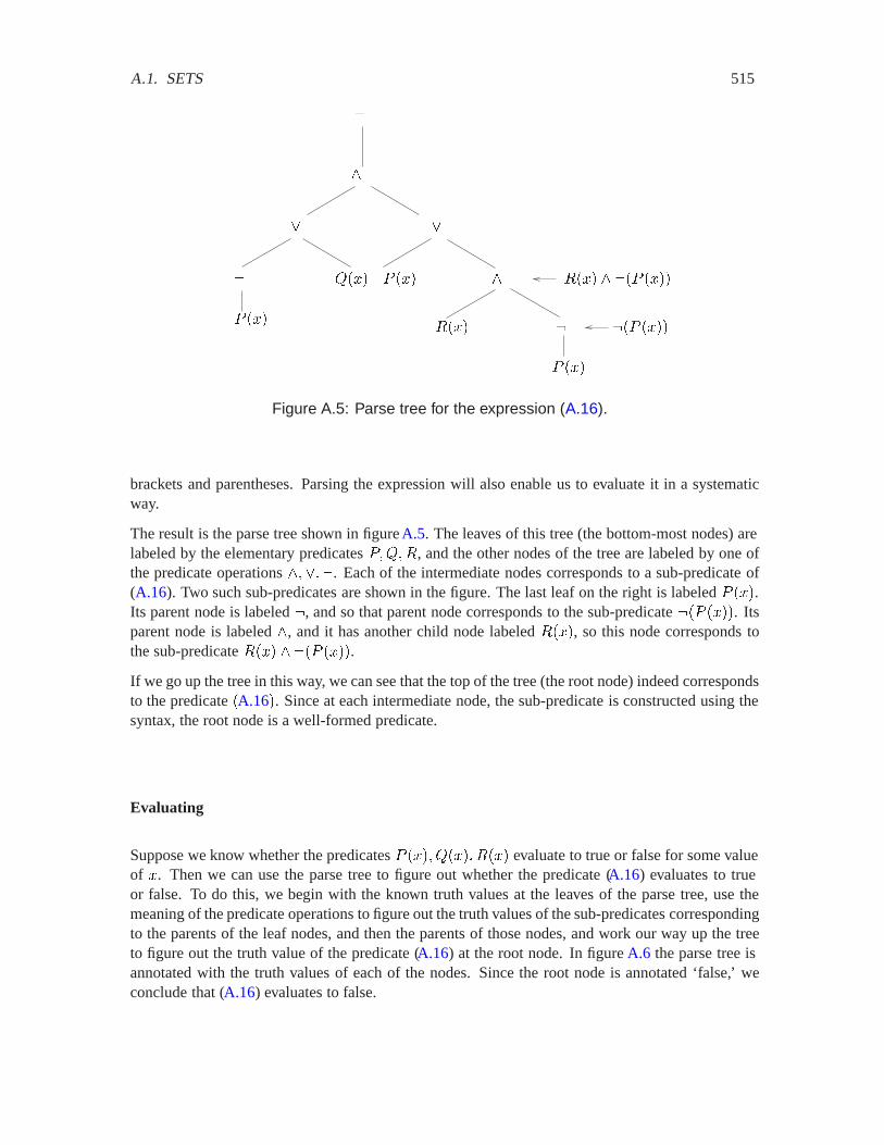
A.1. SETS 515
�
�
�
�
�
� ���
� ���
� �������
G���
��� ����
���� � ��� ����
��
Figure A.5: Parse tree for the expression (A.16).
brackets and parentheses. Parsing the expression will also enable us to evaluate it in a systematicway.
The result is the parse tree shown in figure A.5. The leaves of this tree (the bottom-most nodes) arelabeled by the elementary predicates ��G��, and the other nodes of the tree are labeled by one ofthe predicate operations �����. Each of the intermediate nodes corresponds to a sub-predicate of(A.16). Two such sub-predicates are shown in the figure. The last leaf on the right is labeled � ���.Its parent node is labeled �, and so that parent node corresponds to the sub-predicate ��� ����. Itsparent node is labeled �, and it has another child node labeled ����, so this node corresponds tothe sub-predicate ���� � ��� ����.
If we go up the tree in this way, we can see that the top of the tree (the root node) indeed correspondsto the predicate �A.16�. Since at each intermediate node, the sub-predicate is constructed using thesyntax, the root node is a well-formed predicate.
Evaluating
Suppose we know whether the predicates � ���� G���� ���� evaluate to true or false for some valueof �. Then we can use the parse tree to figure out whether the predicate (A.16) evaluates to trueor false. To do this, we begin with the known truth values at the leaves of the parse tree, use themeaning of the predicate operations to figure out the truth values of the sub-predicates correspondingto the parents of the leaf nodes, and then the parents of those nodes, and work our way up the treeto figure out the truth value of the predicate (A.16) at the root node. In figure A.6 the parse tree isannotated with the truth values of each of the nodes. Since the root node is annotated ‘false,’ weconclude that (A.16) evaluates to false.
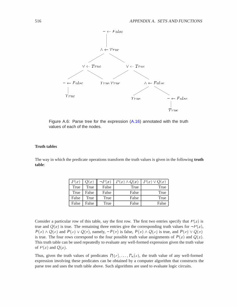
516 APPENDIX A. SETS AND FUNCTIONS
�0�
�0�
�0��0�
�0�
� $ 5�,��
� $ 5�,��
� $ 5�,��
� $ �0�� $ �0�
� $ 5�,��
� $ �0�
Figure A.6: Parse tree for the expression (A.16) annotated with the truthvalues of each of the nodes.
Truth tables
The way in which the predicate operations transform the truth values is given in the following truthtable:
� ��� G��� �� ��� � ��� �G��� � ��� �G���
True True False True TrueTrue False False False TrueFalse True True False TrueFalse False True False False
Consider a particular row of this table, say the first row. The first two entries specify that � ��� istrue and G��� is true. The remaining three entries give the corresponding truth values for �� ���,� ��� � G��� and � ��� � G���, namely, �� ��� is false, � ��� � G��� is true, and � ��� � G���is true. The four rows correspond to the four possible truth value assignments of � ��� and G���.This truth table can be used repeatedly to evaluate any well-formed expression given the truth valueof � ��� and G���.
Thus, given the truth values of predicates ������ � � � � �����, the truth value of any well-formedexpression involving these predicates can be obtained by a computer algorithm that constructs theparse tree and uses the truth table above. Such algorithms are used to evaluate logic circuits.

A.2. FUNCTIONS 517
A.2 Functions
In the notation� � � � $� (A.17)
� and $ are sets, and � is the name of a function. The function is an assignment rule that assignsa value in $ to each element in � . If the element in � is �, then the value is written ����.
We read (A.17) as “� is (the name of) a function from � into (or to) $ .” We also say that � maps� into $ . The set � is called the domain of � , written � � domain���, the set $ is called therange of � , written $ � range���.7 When the domain and range are understood from the context,we write “�” by itself to represent the function or the map. If � is a variable over � , we also say “�is a function of �.”
Example 1.5: Recall the set Studentsof all the students in this class. Each element ofStudentsis represented by a student’s name,
Students� �John Brown� Jane Doe� �We assign to each name in Studentsthe student’s marks in the final examination, anumber between and . This name-to-marks assignment is an example of a func-tion. Just as we give names to sets (e.g. Students), we give names to functions. In thisexample the function might be named Score. When we evaluate the function Scoreatany name, we get the marks assigned to that name. We write this as
Score�John Brown� � �� Score�Jane Doe� � ���� Figure A.7 illustrates the function Score. Three things are involved in defining Score:the set Students, the set �� � of possible marks, and the assignment of marks to eachname. In the figure this assignment is depicted by the arrows: the tail of the arrowpoints to a name and the head of the arrow points to the marks assigned to that name.We denote these three things by
Score�Students� �� �
which we read as “Scoreis a function from Studentsinto �� �.” The domain of thefunction Scoreis Students, and the range of Scoreis �� �.
It is easy to imagine other functions with the same domain Students. For example, Height assignsto each student his or her height measured in cm, SSNassigns students their social security number,and Addressassigns students their address. The range of these functions is different. The range ofHeight might be defined to be �� �� (200 cm is about 6.5 feet). Since a social security numberis a 9-digit number, we can take �� � � �� to be the range of SSN. And we can take the rangeof Addressto be �������, assuming that an address can be expressed as a string of 100 characters,including blank spaces.
7In some mathematics texts, the set ' which we call the range is called the codomain, and range��� is defined to bethe set of all values that � takes, i.e., range��� � ���� � � ��. However, we will not use this terminology.

518 APPENDIX A. SETS AND FUNCTIONS
JohnBrown
JaneDoe
[0, 100]
Students
Figure A.7: Illustration of Score.
We usually use lower case letters for function names, such as �� �� �, or more descriptive namessuch as Score, Voice, Video, SquareWave, AMSignal.
Avoid a bad habit: It is important to distinguish between a function � and its value���� at a particular point � domain���. The function � is a rule that assigns avalue in range��� to each � domain���, whereas ���� is a point or element inrange���. Unfortunately, too many books encourage the bad habit by using ‘����’as a shorthand for ‘� is a function of �.’ If you keep the distinction between � and����, it will be easier to avoid confusion when we study systems.
A.2.1 Defining functions
To define a function, you must give the domain, the range, and the rule that produces an elementin the range given an element in the domain. There are many ways to do this, as explored in muchmore depth in chapter 2. Here we mention only two. The first is enumeration. That is, in tabularform or some other form, each possible value in the domain is associated with a value in the range.This method would be appropriate for the Scorefunction, for example. Alternatively, functions canbe mathematically defined by the prototype: define � � � � $ ,
� � �� ���� � expression in ��
The ‘expression in �’ may be specified by an algebraic expression, by giving the graph of � , by atable, or by a procedure.
A.2. FUNCTIONS 519
A.2.2 Tuples and sequences as functions
An � -tuple � � ���� � �� � �� can be viewed as a function
�� �� � � � ��
For each integer in �� � �, it assigns a value in � . An infinite sequence � over the set $ canalso be viewed as a function
��Naturals� $�
or��Naturals� � $�
depending on whether you wish to begin indexing the sequence at zero or one (both conventions arewidely used). This view of sequences as functions is in fact our model for discrete-time signals andevent traces, as developed in chapter 1.
A.2.3 Function properties
A function � �� � $ is one-to-one if
� �� � and � �� �� �� �� �� � ����� �� ������
Here the logical symbol ‘�’ means ‘implies’ so the expression is read: if ��� �� are two differentelements in � , then ������ ����� are different.
Example 1.6: The function Cube�Reals� Realsgiven by
� � Cube��� � ���
is one-to-one, because if �� �� ��, then ��� �� ���. But Squareis not one-to-one because,for example, Square�� � Square���.
A function � �� � $ is onto if
� � $� � � �� such that ���� � ��
The symbol ‘�’ is the existential quantifier, which means ‘there exists’ or ‘for some’. So the expres-sion above reads: ‘For each � in $ , there exists � in � such that ���� � �.’
Accordingly, � is onto if for every � in its range there is some � in its domain such that � � ����.
Example 1.7: The function Cube�Reals� Realsis one-to-one and onto, whileSquare�Reals� Realsis not onto. However, Square�Reals� Reals� is onto.
520 APPENDIX A. SETS AND FUNCTIONS
Probing further: Infinite sets
The size of a set �, denoted ���, is the number of elements it contains. By counting,we immediately know that �� �� �� � and ��� �� !� � have the same number ofelements, whereas �� �� � has fewer elements. But we cannot count infinite sets.It is more difficult to compare the number of elements in the following infinite sets:
� � Naturals� �� �� �� �� � � � ��� �� �� � � � � �� ��
At first, we might say that � has one more element than �, since � includes � andhas one additional element, �. In fact, these two sets have the same size.
The cardinality of a set is the number of elements in the set, but generalized tohandle infinite sets. Comparing the cardinality of two sets is done by matchingelements, using one-to-one functions. Consider two sets � and �, finite or infinite.We say that � has a smaller cardinality than �, written ��� � ���, if there existsa one-to-one function mapping � into �. We say that � and � have the samecardinality, written ��� � ���, if ��� � ��� and ��� � ���.The cardinality of the infinite set � � Naturals is denoted %�, read “aleph zero”(aleph is the first letter of the Hebrew alphabet). It is quite easy to prove using thedefinition of cardinality that � ) %� for any finite number �.
We can now show that the cardinality of� is also %�. There is a one-to-one function� ��� �, namely
� � �� ���� � �� �
so that ��� � ���, and there is a one-to-one function ��� � �, namely
� � �� ���� � �� �
so that ��� � ���. A similar argument can be used to show that the set of evennumbers and the set of odd numbers also have cardinality %�.
It is more difficult to show that the cardinality of Naturals�Naturalsis also %�. Tosee this, we can define a one-to-one function ��Naturals� � Naturalsas follows(see figure A.8).
���� �� � � ����� �� � �� ����� ��� � �� ���� ��� � �� ���� ��� � ��
Observe that since a rational number '�� can be identified with the pair �'��� Naturals�, the argument above shows that the cardinality of the set of all rationalnumbers is also %�.

A.2. FUNCTIONS 521
Probing further: Even bigger sets
We can show that the cardinality of �� � is strictly larger than that of Naturals; i.e.��� �� 2 �Naturals� Since the function � �Naturals� �� � defined by
� � Naturals� ���� � ��
is one-to-one, we have �Naturals� � ��� ��. However, we can show that there is noone-to-one function in the other direction. If there were such a function �� �� � �Naturals, then it would be possible to enumerate all the elements of �� � in anordered list,
�� � � ���� ��� ��� � (A.18)
(The superscript here is not raising to a power, but just indexing.) We can show thatthis is not possible. If we express each element of �� � by its decimal expansion(ignoring the element 1.0), this list looks like
�� � ��������
��
�� � ��������
��
�� � ��������
��
�� � �����
���
��
Construct any number � �� � with the decimal expansion
� � �������
such that for each &, �� �� ��� where ��� is the &-th term in the decimal expansion of��. Clearly such a number exists and is in �� �. But then for every &, � �� ��, sothat � cannot be in the list ���� ��� ��� . Thus, the list (A.18) is not complete inthat it does not include all the elements of �� �.
The cardinality of �� � is denoted %�, and is strictly greater than %�. In this sensewe can say that the continuum �� � has more elements than the denumerable setNaturals, even though both sets have infinite size.
The obvious question is whether there are cardinalities larger than %�. The answeris yes; in fact, there are sets of ever higher cardinality,
%� ) %� ) %��
and sets with cardinality larger than all of these!
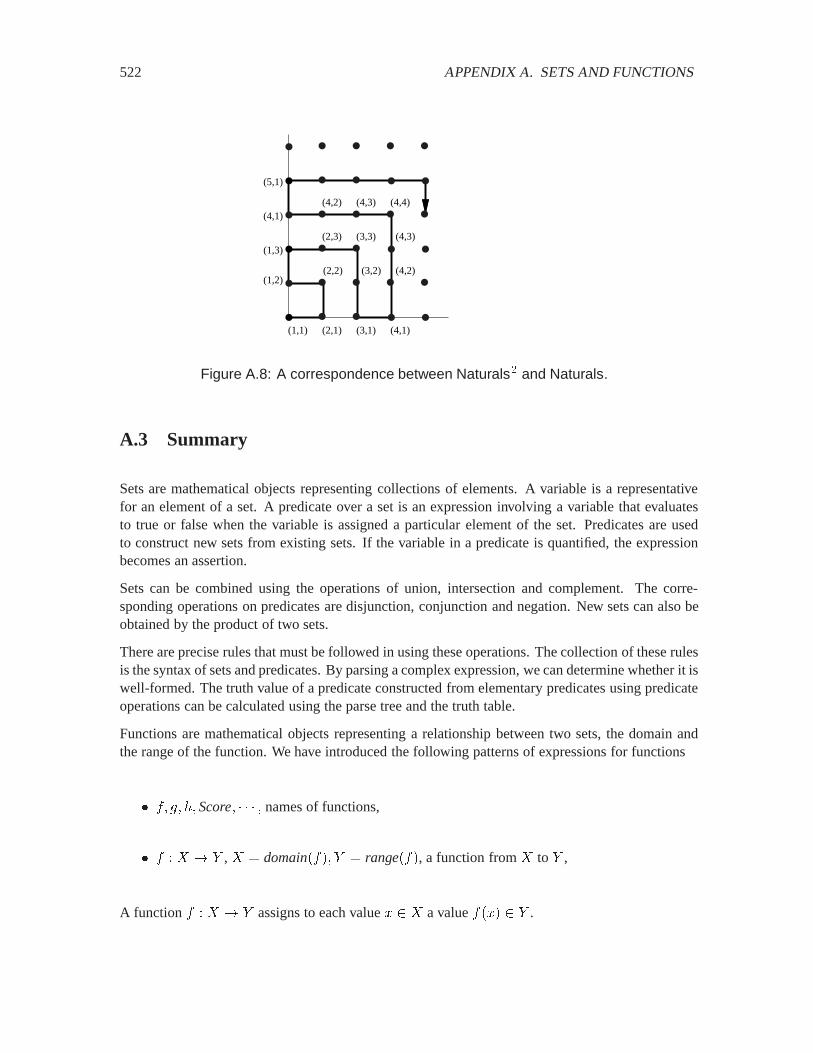
522 APPENDIX A. SETS AND FUNCTIONS
(1,1)
(2,2)(1,2)
(2,1)
(1,3)(2,3) (3,3)
(3,2)
(3,1) (4,1)
(4,2)
(4,3)
(4,4)(4,3)(4,2)(4,1)
(5,1)
Figure A.8: A correspondence between Naturals� and Naturals.
A.3 Summary
Sets are mathematical objects representing collections of elements. A variable is a representativefor an element of a set. A predicate over a set is an expression involving a variable that evaluatesto true or false when the variable is assigned a particular element of the set. Predicates are usedto construct new sets from existing sets. If the variable in a predicate is quantified, the expressionbecomes an assertion.
Sets can be combined using the operations of union, intersection and complement. The corre-sponding operations on predicates are disjunction, conjunction and negation. New sets can also beobtained by the product of two sets.
There are precise rules that must be followed in using these operations. The collection of these rulesis the syntax of sets and predicates. By parsing a complex expression, we can determine whether it iswell-formed. The truth value of a predicate constructed from elementary predicates using predicateoperations can be calculated using the parse tree and the truth table.
Functions are mathematical objects representing a relationship between two sets, the domain andthe range of the function. We have introduced the following patterns of expressions for functions
� �� �� ��Score� � names of functions,
� � � � � $ , � � domain���� $ � range���, a function from � to $ ,
A function � � � � $ assigns to each value � � a value ���� $ .

A.3. SUMMARY 523
Exercises
Each problem is annotated with the letter E, T, C which stands for exercise, requires some thought,requires some conceptualization. Problems labeled E are usually mechanical, those labeled T re-quire a plan of attack, those labeled C usually have more than one defensible answer.
1. E In the spirit of figure A.2, give a picture of the following sets:
(a) �� �� �,(b) �� � � �� ,(c) �� � � ��� ��.
(d) �� �� � � ��� �,(e) ��� � � �� �.
2. E How many elements are there in the sets (a) �� � , (b) ������ � , and (c)�� � � � ��� �?
3. T Determine which of the following expressions is true and which is false:
(a) �� Naturals� � 2 ,
(b) �� Naturals� � ) ,
(c) If � � �� �� � and � � ��� �� � , then �� ���� �� � � �,
(d) If � � �� �� � and � � ��� �� � , then �� ���� �� � � �,
(e) If � � �� �� � and � � ��� �� � , then �� ���� �� � � �.
4. T In the following figure, � � ���� �� � �� � �� � is depicted as a 2-dimensional circleand % � �� �� is shown as a 1-dimensional line segment. Explain why it is reasonable toshow the product set as a 3-dimensional cylinder.
% �
� � %
5. E In the spirit of figure A.2, give a picture for the product set �3�0�7� �� 5����� ���and indicate on your drawing the lecture hours for this class.
6. E In the spirit of figure A.2, give a picture for the set � � ���� �� � � �� ��� � �� �� andthe set � � ���� �� � � �� ��. Explain why the two sets are different.
524 APPENDIX A. SETS AND FUNCTIONS
7. C Give a precise expression for the predicate below so that Triangle is indeed a triangle:
Triangle� ���� �� Reals� � Pred��� ���
There are many ways of writing this predicate. One way is to express Pred��� �� as theconjunction of three linear inequality predicates. Hint: We used the conjunction of two linearinequality predicates in figure A.4.
8. T If � has ' elements and $ has � elements, how many elements are there in � �$ ? If ��
has '� elements, for & � � � � , for some constant � . How many elements are there in
��5/���
�� � �� � ��5(
9. T How many different 10-letter strings are there if each letter is drawn from the set �,(����consisting of the 26 lower case letters of the alphabet? How many such strings are there withexactlyone occurrence of the letter �?
10. T Recall that a set cannot contain duplicate elements. Now suppose � contains 10 elements.
� How many two-element combinations of elements from � are there?
� How many two-element permutations are there?
11. C Construct predicates for use in the prototype (A.4) to define the following sets. Define themin terms of examples of sets introduced in this chapter.
(a) The set of U.S. cities with a population exceeding one million.
(b) The male students in the class.
(c) The old books in the library.
12. T Which of the following expressions is well formed? For those that are well formed, statewhether they are assertions. For those that are assertions, evaluate the assertion to true orfalse. For those that are not assertions, find an equivalent simpler expression.
(a) � �� �� �,(b) � � �� �� �,(c) �� � �� �� �,(d) � � �� �� �,(e) �� � �� �� �,(f) ����� ���� � �� Reals� ��� � � � ���,(g) �� Reals� � 2 � � � ) �,(h) �� �� � ��� �� � �.
13. E Define the following sets in terms of the sets named in sectionA.1.5
(a) The set of all 10-letter passwords.
A.3. SUMMARY 525
(b) The set of all �� matrices of real numbers.
(c) The set of all complex numbers with magnitude at most 1.
(d) The set of all 2-dimensional vectors with magnitude exactly 1.
14. E Give the set of all subsets � ��� of the set � � ��� �� !.15. T Suppose a set � has � elements. Let � ��� be the power set of � . How many elements
are there in � ���?
16. T Use Matlab to depict the following sets using the plot command:
(a) ��� �� Reals� � � � ������ and �� ������
������ � ������,
(b) ���� �� Reals� � � � ��� and � ���� � ��� �� � �
�� � � ,(c) ���� �� Reals� � � � ���� and � ���� � �
�� �� � ��� � � �
17. T Determine which of the following functions is onto, which is one-to-one, and which isneither, and give a short explanation for your answer.
(a) License�CalVehicles� ����� given by � vehicle CalVehicles,License�vehicle� is the California license number of the vehicle
(b) � �Reals� ���� ��, given by � � Reals� ���� � � ������
(c) � �Reals� Reals, given by � � Reals� ���� � � ������
(d) conj�Complex� Complex, the complex conjugate function
(e) � �Complex� Reals�, given by � � Complex� ���� � ������� �'����, where����� is the real part of � and �'��� is the imaginary part of �.
(f) 3 �Reals� � Reals�� � ���� ��� Reals�,
3���� ��� � ���� ���
where ����
� ��
��
����
��
(g) Zero � Reals � Reals�� � Reals� Zero��� � �� � � �
18. T Let �, �, and � be arbitrary sets. Let � �� � � and ��� � � be two functions withdomain and range �. Which of the following assertions is true for all choices of �, �, � , � ,and �?
(a) �� ��� # � � �� # �� � �� # ��.
(b) � �� ��� � � ��� � � ���.
(c) � Æ � � � Æ � .
(d) If both � and � are one-to-one, then � Æ � is one-to-one.
Note that � Æ � is function composition, defined in section2.1.5. � # $ is the complement of$ in � , as explained in section A.1.6. � ��� is the power set of � , as explained in sectionA.1.2.
526 APPENDIX A. SETS AND FUNCTIONS
19. E Each of the following expressions is intended to be a predicate expression. Determinewhether it is true or false, or whether it is not well formed, or has a free variable. If it has afree variable, identify the free variable.
(a) � sets �� � � � ���, where � ��� is the power set of �.
(b) � � Reals� �� Integers��� � � .(c) � � Naturals� � � �� ��� �� � �� �� �� .
(d) �� Naturals� �� � � .
Appendix B
Complex Numbers
Complex numbers are used extensively in the modeling of signals and systems for two reasons.The first reason is that complex numbers provide a compact and elegant way to talk simultaneouslyabout the phase and amplitude of sinusoidal signals. Complex numbers are therefore heavily usedin Fourier analysis, which represents arbitrary signals in terms of sinusoidal signals. The secondreason is that a large class of systems, called linear time-invariant (LTI) systems, treat signals thatcan be described as complex exponential functions in an especially simple way. They simply scalethe signals.
These uses of complex numbers are developed in detail in the main body of this text. This appendixsummarizes essential properties of complex numbers themselves. We review complex number arith-metic, how to manipulate complex exponentials, Euler’s formula, the polar coordinate representa-tion of complex numbers, and the phasor representation of sinewaves.
B.1 Imaginary numbers
The quadratic equation,�� � � �
has two solutions, � � � and � � �. These solutions are said to be roots of the polynomial�� � . Thus, this polynomial has two roots, � and �.
More generally, the roots of the �-th degree polynomial,
�� � ������ � � ������ ��� (B.1)
are defined to be the solutions to the polynomial equation
�� � ������ � � ������ �� � � (B.2)
The roots of a polynomial provide a particularly useful factorization into first-degree polynomials.For example, we can factor the polynomial �� � as
�� � � ��� ���� ��
527
528 APPENDIX B. COMPLEX NUMBERS
Notice the role of the roots, � and �. In general, if (B.1) has roots ��� � ��, then we can factorthe polynomial as follows
�� � ������ � � ������ �� � ��� ������ ��� ��� ���� (B.3)
It is easy to see that if � � �� for any & �� �, then the polynomial evaluates to zero, so (B.2)is satisfied.
This raises the question whether (B.2) always has a solution for �. In other words, can we alwaysfind roots for a polynomial?
The equation�� � � (B.4)
has no solution for � in the set of real numbers. Thus, it would appear that not all polynomials haveroots. However, a surprisingly simple and clever mathematical device changes the picture dramat-ically. With the introduction of imaginary numbers, mathematicians ensure that all polynomialshave roots. Moreover, they ensure that any polynomial of degree � has exactly � factors as in (B.3).The � values ��� � �� (some of which may be repeated) are the roots of the polynomial.
If we try by simple algebra to solve (B.4) we discover that we need to find � such that
�� � ��This suggests that
� ����
But � does not normally have a square root.
The clever device is to define an imaginary number, usually written & or , that is equal to��. By
definition,1
&� & ������ � ��
This (imaginary) number, thus, is a solution of the equation �� � � .
For any real number �, &� is an imaginary number. Thus, we can define the set of imaginary numbersas
ImaginaryNumbers� �&� � � Reals� and & ��� (B.5)
It is a profound result that this simple device is all we need to guarantee that every polynomialequation has a solution, and that every polynomial of degree � can be factored into � polynomialsof degree one, as in (B.3).
B.2 Arithmetic of imaginary numbers
The sum of & (or &) and & is written &�. Sums and differences of imaginary numbers simplify likereal numbers:
&� � &� � &�� &�� &� � �&�1Here, the operator � is ordinary multiplication, not products of sets.

B.3. COMPLEX NUMBERS 529
If &�� and &�� are two imaginary numbers, then
&�� � &�� � &��� � ���� &�� � &�� � &��� � ���� (B.6)
The product of a real number � and an imaginary number &� is
�� &� � &� � � � &���
To take the product of two imaginary numbers, we must remember that &� � �, and so for any twoimaginary numbers, &�� and &��, we have
&�� � &�� � ��� � ��� (B.7)
The result is a real number. We can use rule (B.7) repeatedly to multiply as many imaginary numbersas we wish. For example,
&� & � �� &� � &� &� � �&� & � �
The ratio of two imaginary numbers &�� and &�� is a real number
&��&��
�����
�
B.3 Complex numbers
The sum of a real number � and an imaginary number &� is called a complex number. This sumdoes not simplify as do the sums of two reals numbers or two imaginary numbers, and it is writtenas �� &� or �� �.
Examples of complex numbers are
� � &� ��� &�� �� � &���
In general a complex number � is of the form
� � �� &� � ������
where �� � are real numbers. The real part of �, written Re��, is �. The imaginary part of �,written Im��, is �. Notice that, confusingly, the imaginary part is a real number.The imaginarypart times & is an imaginary number. So
� � Re��� &Im���The set of complex numbers, therefore, is defined by
Complex� ��� &� � � Reals� � Reals� and & ���� (B.8)
Every real number � is in Complex, because � � � � &; and every imaginary number &� is inComplex, because &� � � &�.
Two complex numbers �� � �� � &�� and �� � �� � &�� are equal if and only if their real parts areequal and their imaginary parts are equal, i.e. �� � �� if and only if
Re��� � Re���� and Im��� � Im����

530 APPENDIX B. COMPLEX NUMBERS
B.4 Arithmetic of complex numbers
In order to add two complex numbers, we separately add their real and imaginary parts,
��� � &��� � ��� � &��� � ��� � ��� � &��� � ����
The complex conjugate of � � &� is defined to be � � &�. The complex conjugate of a complexnumber � is written ��. Notice that
� � �� � �Re��� � � �� � �&Im���Hence, the real and imaginary parts can be obtained using the complex conjugate,
Re�� � � � ��
�� and Im�� � � � ��
�&�
The product of two complex numbers works as expected if you remember that &� � �. So, forexample,
� � �&��� � �&� � � � �&� �&� &� � � � �&� � �� � �&�
which seems strange, but follows mechanically from &� � �. In general,
��� � &������ � &��� � ����� � ����� � &����� � ������ (B.9)
If we multiply � � �� &� by its complex conjugate �� we get
��� � ��� &����� &�� � �� � ���
which is a positive real number. Its positive square root is called the modulus or magnitude of �,and is written ���,
��� ����� �
��� � �� �
How to calculate the ratio of two complex numbers is less obvious, but it is equally mechanical. Weconvert the denominator into a real number by multiplying both numerator and denominator by thecomplex conjugate of the denominator,
� � �&
� �&�
� � �&
� �&� � �&
� �&
��� � � � ��� � ��&
� �
��
��
�&�
The general formula is
�� � &���� � &��
����� � ������� � ���
� &����� � ����
��� � ���� (B.10)
In practice it is easier to calculate the ratio as in the example, rather than memorizing formula(B.10).
B.5. EXPONENTIALS 531
B.5 Exponentials
Certain functions of real numbers, like the exponential function, are defined by an infinite series.The exponential of a real number �, written �� or )$*���, is
�� ������
��
6�� � ��
��
�����
��� �
We also recall the infinite series expansion for ��� and ���:
����#� � � #�
��#
���
����#� � # � #�
���#�
���
The exponential of a complex number � is written �� or )$*���, and is defined in the same way asthe exponential of a real number,
�� ������
��
6�� � � �
��
�����
��� � (B.11)
Note that �� � , as expected.
The exponential of an imaginary number &# is very interesting,
��* � � �&#� ��&#��
���
�&#��
���
� �� #�
��#
��� � � &�# � #�
���#�
��� �
� ����#� � & ����#��
This identity is known as Euler’s formula:
��* � ����#� � & ����#�� (B.12)
Euler’s formula is used heavily in this text in the analysis of linear time invariant systems. It allowssinusoidal functions to be given as sums or differences of exponential functions,
����#� � ���* � ���*��� (B.13)
and����#� � ���* � ���*����&�� (B.14)
This proves useful because exponential functions turn out to be simpler mathematically (despitebeing complex valued) than sinusoidal functions.
An important property of the exponential function is the product formula:
������ � ������ � (B.15)
532 APPENDIX B. COMPLEX NUMBERS
We can obtain many trigonometric identities by combining (B.12) and (B.15). For example, since
��*���* � ��*��* � �� � �
and��*���* � �����#� � & ����#�������#�� & ����#�� � �����#� � �����#��
so we have the identity
�����#� � �����#� � �
Here is another example. Using�� 3�6� � ��3��6� (B.16)
we get
����*� +� � & ����*� +� � �����*� � & ����*�������+� � & ����+��
� �����*� ����+�� ����*� ����+��
�&�����*� ����+� � ����*� ����+���
Since the real part of the left side must equal the real part of the right side, we get the identity,
����*� +� � ����*� ����+�� ����*� ����+��
Since the imaginary part of the left side must equal the imaginary part of the right side, we get theidentity,
����*� +� � ����*� ����+� � ����*� ����+��
It is much easier to remember (B.16) than to remember these identities.
B.6 Polar coordinates
The representation of a complex number as a sum of a real and an imaginary number, � � � � &�,is called its Cartesian representation.
Recall from trigonometry that if �� �� � are real numbers and �� � �� � ��, then there is a uniquenumber # with � # ) �� such that
����#� ��
�� ����#� �
�
��
That number is# � ���������� � ���������� � �����������
We can therefore express any complex number � � �� &� as
� � ���� ���� � &�
��� � � ������� # � & ��� #� � �����* �

B.6. POLAR COORDINATES 533
Basics: From Cartesian to polar coordinates
Since ����� is multi-valued, you must be careful in calculating ����������, when� is negative. For any H Reals, define �������H� to be the unique number in������ ���� such that �����������H�� � H. Then,
����� �
������������� if � � � � ������������ if � )
Im
Re
z = x + iy
θ
r
x
y
Figure B.1: A complex number � is represented in Cartesian coordinatesas � � �� &� and in polar coordinates as � � ���*. The �-axis is called thereal axis, the � axis is called the imaginary axis. The angle # in radians ismeasured counter-clockwise from the real axis.
where # � ����������. The angle or argument # is measured in radians, and it is written as ��&���or � �. So we have the polar representation of any complex number � as
� � �� &� � ���*� (B.17)
The two representations are related by
� � ��� ���� � ��
and# � ��&��� � �����������
The values � and � are called the Cartesian coordinates of �, while � and # are its polar coordi-nates. Note that � is real and � � .
Figure B.1 depicts the Cartesian and polar representations. Note that for any integer > ,
��� ��)�*� � ���*�
This is because��� ��)�*� � �����)��*

534 APPENDIX B. COMPLEX NUMBERS
and����) � �����>�� � & �����>�� � �
Thus, the polar coordinates ��� #� and ��� # � �>�� for any integer > represent the same complexnumber. Thus, the polar representation is not unique; by convention, a unique polar representationcan be obtained by requiring that the angle given by a value of # satisfying � # ) �� or �� )# � �. We normally require � # ) ��.
Example 2.1: The polar representation of the number is � ���. Notice that it isalso true that � ���) , because the sine and cosine are periodic with period ��. Thepolar representation of the number � is � � ��) . Again, it is true that � � ���) ,or, in fact, � � ��)���) , for any integer > .
Products of complex numbers represented in polar coordinates are easy to compute. If �� � ������*� ,then
���� � ���������� *��*���
Thus the magnitude of a product is a product of the magnitudes, and the angle of a product is thesum of the angles,
������ � ��������� � ������ � � ���� � � �����
Example 2.2: We can use the polar representation to find the � distinct roots of theequation �� � . Write � � ���*, and � ���) , so
�� � �����* � ����)�
which gives � � and # � �6���, 6 � � � � � � . These are called the � rootsof unity. Figure B.2 shows the 5 roots of unity.
Whereas it is easy to solve the polynomial equation �� � , solving a general polynomial equationis difficult.
Theorem The polynomial equation
�� � ������ � � ����� � �� � �
where ��� � �� are complex constants, has exactly � factors of the form �� � *��,where *�� *� are called the � roots. In other words, we can always find the factor-ization,
�� � ������ � � ����� � �� �
�/���
�� � *�� �
Some of the roots may be identical.
Note that although this theorem ensures the existence of this factorization, it does not suggest a wayto find the roots. Indeed, finding the roots can be difficult. Fortunately, software for finding roots isreadily available, for example using the Matlab roots function.
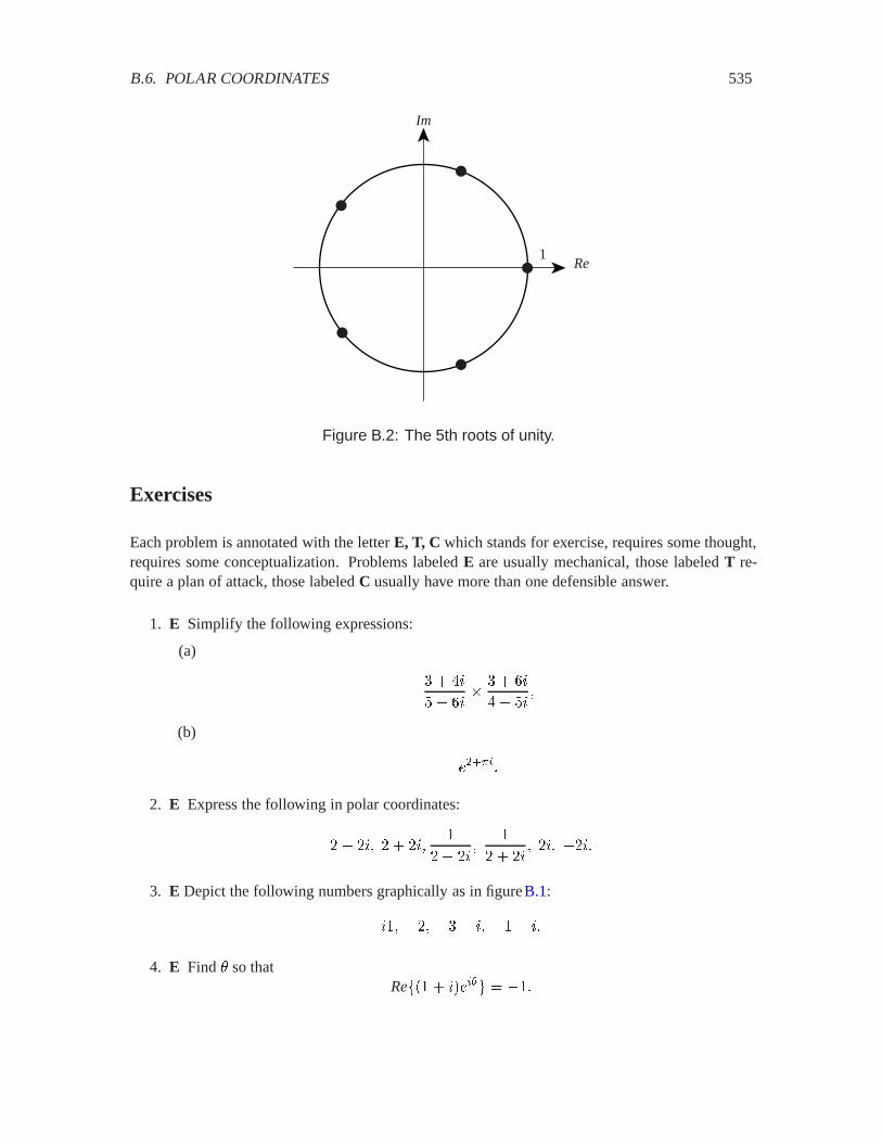
B.6. POLAR COORDINATES 535
Im
Re1
Figure B.2: The 5th roots of unity.
Exercises
Each problem is annotated with the letter E, T, C which stands for exercise, requires some thought,requires some conceptualization. Problems labeled E are usually mechanical, those labeled T re-quire a plan of attack, those labeled C usually have more than one defensible answer.
1. E Simplify the following expressions:
(a)
� � �&
�� &� � � &
�� �&�
(b)
���)��
2. E Express the following in polar coordinates:
�� �&� � � �&�
�� �&�
� � �&� �&� ��&�
3. E Depict the following numbers graphically as in figureB.1:
&� ��� ��� &� �� &�
4. E Find # so thatRe�� � &���* � ��
536 APPENDIX B. COMPLEX NUMBERS
5. E Express the six distinct roots of unity, i.e. the six solutions to
�� �
in Cartesian and polar coordinates.
6. T Express the six roots of �, i.e. the six solutions to
�� � �
in Cartesian and polar coordinates. Depict these roots as in FigureB.2.
7. T Figure out &� for all positive and negative integers �. (For a negative integer �, ��� ����.)
8. T Factor the polynomial �� � � as
�� � � ��/
���
�� � *���
expressing the *� in polar coordinates.
9. C How would you define� � & ? More generally, how would you define
�� for any
complex number �?
10. T The logarithm of a complex number � is written !�& � or !�&��� . It can be defined as aninfinite series, or as the inverse of the exponential, i.e. define !�& � � /, if �7 � �. Using thelatter definition, find the logarithm of the following complex numbers:
� �� &� �&� � &
More generally, if � �� is expressed in polar coordinates, what is !�& �? For which complexnumbers � is !�& � not defined?
11. E Use Matlab to answer the following questions. Let �� � ���& and �� � ���&. Hint: Con-sult Matlab help on i, j, exp, real, imag, abs, angle, conj, and complex. Lookingup “complex” in the help desk may also be helpful.
(a) What is �� � ��? What are the real and imaginary parts of the sum?
(b) Express the sum in polar coordinates.
(c) Draw by hand two rays in the complex plane, one from the origin to �� and the otherfrom the origin to ��. Now draw �� � �� and �� � �� on the same plane. Explain howyou might systematically construct the sum and difference rays.
(d) Draw two rays in the complex plane to �� � ����& and � � ���&. Now draw ����and ����.
(e) Consider �� � ���)�� and �� � ��� . Express �� in polar coordinates. What is ����?
(f) Draw the ray to �� � � &. Now draw rays to �� � �����)� for � � � �� �� � � �. How
many distinct �� are there?

B.6. POLAR COORDINATES 537
(g) Find all the solutions of the equation �� � . Hint: Express � in polar coordinates,� � ���* and solve for �� #.
12. E This problem explores how complex signals may be visualized and analyzed.
(a) Use Matlab to plot the complex exponential function as follows:
plot(exp((-2+10i)*[0:0.01:1]))
The result is a spiraling curve corresponding to the signal � � �� �� Complexwhere
� �� � ��� � � ���������
In the plot window, under the Tools menu item, use ‘Axes properties’ to turn on the grid.Print the plot and on it mark the points for which the function is purely imaginary. Is itevident what values of yield purely imaginary ���?
(b) Find analytically the values of that result in purely imaginary and purely real ���.
(c) Construct four plots, where the horizontal axis represents and the vertical axis repre-sents the real and imaginary parts of ���, and the magnitude and angle of ���. Givethese as four subplots.
(d) Give the mathematical expressions for the four functions plotted above in part (c).
13. T Euler’s formula is: for any real number #,
��* � ��� # � & ��� #�
and the product formula is: for any complex numbers ��� ��,
������ � ������ �
The following problems show that these two formulas can be combined to obtain many usefulidentities.
(a) Express �����#� and �����#� as sums and products of ��� # and ��� #. Hint: Write���* � ��*��* (by the product formula) and then use Euler’s formula.
(b) Express �����#� and �����#� also as sums and products of ��� # and ��� #.
(c) The sum of several sinewaves of the samefrequency � but different phases is a sinewaveof the same frequency, i.e. given ��� <�, 6 � � � � � � �, we can find ��< so that
� ������ <� ���
���
�� ������ <��
Express ��< in terms of ���� <�.

538 APPENDIX B. COMPLEX NUMBERS

Appendix C
Laboratory Exercises
This appendix contains laboratory exercises based on Matlab and Simulink. The purpose of theseexercises is to help reconcile the declarative (what is) and imperative (how to) points of view onsignals and systems. The mathematical treatment that dominates in the main body of this text isdeclarative, in that it asserts properties of signals and studies the relationships between signals thatare implied by systems. This appendix focuses on an imperative style, where signals and systemsare constructed procedurally.
Matlab and Simulink, distributed by The MathWorks, Inc., are chosen as the basis for these exercisesbecause they are widely used by practitioners in the field, and because they are capable of realizinginteresting systems. Why use both Matlab and Simulink? Although they are integrated into a singlepackage, Matlab and Simulink are two very different pieces of software with radically differentapproaches to modeling of signals and systems. Matlab is an imperative programming language,whereas Simulink is a block diagram language. In Matlab, one specifies the sequence of steps thatconstruct a signal or operate on a signal to produce a new signal. In Simulink, one connects blocksthat implement elementary systems to construct more interesting systems. The systems we constructare aggregates of simpler systems.
Matlab fundamentally operates on matrices and vectors. Simulink fundamentally operates on dis-crete and continuous-time signals. Discrete-time signals, of course, can be represented as vectors.Continuous-time signals, however, can only be approximated. Simulink, since it is a computer pro-gram, must of course approximate continuous-time signals as well by discretizing time. But thatapproximation is largely transparent, and the user (the model builder) can pretend that he or she isoperating directly on continuous-time signals.
There is considerable value in becoming adept with these software packages. Matlab and Simulinkare often used in practice for “quick-and-dirty” prototyping of concepts. In a matter of a few hours,very elaborate models can be constructed. This contrasts with the weeks or months that would oftenbe required to build a hardware prototype to test the same concept.
Of course, a conventional programming language such as C++ or Java could also be used to con-struct prototypes of systems. However, these languages lack the rich libraries of built-in functionsthat Matlab and Simulink have. A task as conceptually simple as plotting a waveform can take
539
540 APPENDIX C. LABORATORY EXERCISES
weeks of programming in Java to accomplish well. Algorithms, such as the FFT or filtering algo-rithms, are also built in, saving considerable effort.
Matlab and Simulink both have capabilities that are much more sophisticated than anything coveredin this text. This may be a bit intimidating at first (“what the heck is singular-value decomposi-tion!?!?!?”). In fact, these tools are rich enough in functionality to keep you busy for an entirecareer in engineering. You will need to learn to ignore what you don’t understand, and focus onbuilding up your abilities gradually.
If you have no background in programming, these exercises will be difficult at first. Matlab, at itsroot, is a fairly conventionally programming language, and it requires a clear understanding of pro-gramming concepts such as variables and flow of control (for loops, while loops). As programminglanguages go, it is an especially easy one to learn, however. Its syntax (the way commands are writ-ten) is straightforward and close to that of the mathematical concepts that it emulates. Moreover,since it is an interpreted language (in contrast to a compiled language), you can easily experimentby just typing in commands at the console and seeing what happens. Be fearless! The worst thatcan happen is that you will have to start over again.
These labs assume the computer platform is Microsoft Windows, although any platform capable ofrunning Matlab and Simulink will work, as long as it has full support for sound and images.
Mechanics of the labs
The labs are divided into two distinct sections, in lab and independent. The purpose of the in-labsection is to introduce concepts needed for later parts of the lab. Each in-lab section is designed tobe completed during a scheduled lab time with an instructor present to clear up any confusing orunclear concepts. The in-lab section is completed by obtaining the signature of an instructor on averification sheet.
The independent section begins where the in-lab section leaves off. It can be completed within thescheduled lab period, or may be completed on your own time. You should write a brief summaryof your solution to the lab exercise and turn it in at the beginning of the next scheduled lab period.Your summary should clearly answer each question posed in the independent section of the lab.
The lab writeup should be kept simple. It must include the names of the members of the group (ifthe lab is done by a group), the time of the lab section, the name of the lab, and the date. It shouldthen proceed to give clear answers to each of the questions posed by the lab. Matlab code should beprovided in a fixed width font (Courier New, 10pt, for example) and plots should be clearly labeledand referenced in the writeup. Plots may be included directly in the flow of the analysis. If includedon a separate page, two to eight plots should be placed on the same page, depending on the natureof the plots. You can copy Matlab plots into most word processors using the Copy Figure commandin the Edit menu.
Here is an example of a response to a portion of a lab:
2. Simple Low Pass Filter
Figure C.1 shows the data before (top) and after (bottom) the low pass filter. The low
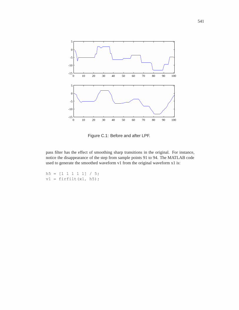
541
0 10 20 30 40 50 60 70 80 90 100 -15 -10
-5 0
5
0 10 20 30 40 50 60 70 80 90 100 -15 -10
-5 0 5
Figure C.1: Before and after LPF.
pass filter has the effect of smoothing sharp transitions in the original. For instance,notice the disappearance of the step from sample points 91 to 94. The MATLAB codeused to generate the smoothed waveform v1 from the original waveform x1 is:
h5 = [1 1 1 1 1] / 5;v1 = firfilt(x1, h5);
542 APPENDIX C. LABORATORY EXERCISES
C.1 Arrays and sound
The purpose of this lab is to explore arrays in Matlab and to use them to construct sound signals. Thelab is designed to help you become familiar with the fundamentals of Matlab. It is self contained,in the sense that no additional documentation for Matlab is needed. Instead, we rely on the on-linehelp facilities. Some people, however, much prefer to sit down with a tutorial text about a piece ofsoftware, rather than relying on on-line help. There are many excellent books that introduce Matlab.Check your local bookstore or The MathWorks’ website (http://www.mathworks.com/).
Note that there is some potential confusion because Matlab uses the term “function” somewhatmore loosely than we do when we refer to mathematical functions. Any Matlab command that takesarguments in parentheses is called a function. And most have a well-defined domain and range,and do, in fact, define a mapping from the domain to the range. These can be viewed formally as a(mathematical) functions. Some, however, such as plot and sound are a bit harder to view thisway. The last exercise here explores this relationship.
C.1.1 In-lab section
To run Matlab simply double click on the Matlab icon on the desktop, or find the Matlab commandin the start menu. This will open a Matlab command window, which displays a prompt “>>”. Youtype commands at the prompt. Explore the built-in demos by typing demo.
Matlab provides an on-line help system accessible by using the help command. For example, toget information about the function size, enter the following:
>> help size
There also is a help desk (formatted in HTML for viewing from a web browser) with useful intro-ductory material. It is accessed from the Help menu. If you have no prior experience with Matlab,see the topic “Getting Started” in the help desk. Spend some time with this. You can find in the helpdesk all the information you need to carry out the following exercises.
1. A variable in Matlab is an array. An array has dimensions � �3 , where � and 3 are inNaturals. � is the number of rows and 3 is the number of columns. If � � 3 � , thevariable is a scalar. If � � and 3 2 , then the variable is a row vector. If � 2 and3 � , then the variable is a column vector. If both � and 3 are greater than one, then thevariable is a matrix, and if � � 3 then the variable is a square matrix. The coefficients ofan array are real or complex numbers.
(a) Each of the following is an assignment of a value to a variable called array. For each,identify the dimensions of the array (3 and � ), and identify whether the variable is ascalar, row vector, column vector, or matrix.
array = [1 2 3 4 5]array = [1:5]
C.1. ARRAYS AND SOUND 543
array = 1:5array = [1:1:5]array = [1:-1:-5]array = [1 2; 3 4]array = [1; 2; 3; 4]
(b) Create a � � � matrix containing arbitrary data. Explore using the Matlab functionszeros, ones, eye, and rand to create the matrix. Find a way to use the squarematrix eye(2) as part of your � � � matrix. Verify the sizes of your arrays usingsize.
(c) Use the Matlab commands size and length to determine the length of the arraysgiven by 1:0.3:10 and 1:1:-1. Consider more generally the array constructor pat-tern
array = start : step : stop
where start, stop, and step are scalar variables or real numbers. How many el-ements are there in array? Give an expression in Matlab in terms of the variablesstart, stop, and step. That is, we should be able to do the following:
>> start = 1;>> stop = 5;>> step = 1;>> array = start:step:stop;
and then evaluate your expression and have it equal length(array). (Notice thatthe semicolons at the end of each command above suppress Matlab’s response to eachcommand.) Hint: to get a general expression, you will need something like the floorfunction. Verify your answer for the arrays 1:0.3:10 and 1:1:-1.
2. Matlab can be used as a general-purpose programming language. Unlike a general-purposeprogramming language, however, it has special features for operating on arrays that make itespecially convenient for modeling signals and systems.
(a) In this exercise, we will use Matlab to compute
������
6�
Use a for loop (try help for) to specify each individual addition in the summation.
(b) Use the sum function to give a more compact, one-line specification of the sum inpart (a). The difference between these two approaches illustrates the difference betweenusing Matlab and using a more traditional programming language. The for loop is closerto the style one would use with C++ or Java. The sum function illustrates what Matlabdoes best: compact operations on entire arrays.
(c) In Matlab, any built-in function that operates on a scalar can also operate on an array.For example,
544 APPENDIX C. LABORATORY EXERCISES
>> sin(pi/4)
ans =
0.7071
>> sin([0 pi/4 pi/2 3*pi/4 pi])
ans =
0 0.7071 1.0000 0.7071 0.0000
This feature is called vectorization. Use vectorization to construct a vector that tabu-lates the values of the sin function for the set �� ��� ���� � �. Use the colonnotation explored in the previous exercise.
(d) Given two arrays A and B that have the same dimensions, Matlab can multiply the ele-ments pointwise using the .* operator. For example,
>> [1 2 3 4].*[1 2 3 4]
ans =
1 4 9 16
Use this pointwise multiply to tabulate the values of �&�� for the set
�� ��� ���� � ��
3. A discrete-time signal may be approximated in Matlab by a vector (either a row or a columnvector). In this exercise, you build a few such vectors and plot them.
(a) Create an array that is a row vector of length 36, with zeros everywhere except in the18th position, which has value 1. (Hint: try help zeros to find a way to create arow vector with just zeros, and then assign the 18-th element of this vector the valueone.) This array approximates a discrete-time impulse, which is a signal that is zeroeverywhere except at one sample point. We will use impulses to study linear systems.Plot the impulse signal, using both plot and stem.
(b) Sketch by hand the sine wave � � ��� �� Reals, given by
� ��� �� ��� � ������ � �� �� ��
In your sketch carefully plot the value at time 0. Assume the domain represents timein seconds. What is the frequency of this sine wave in Hertz and in radians per second,what is its period in seconds, and how many complete cycles are there in the interval��� �?
(c) Sample the function � from the previous part at 8 kHz, and using Matlab, plot thesamples for the entire interval ��� �. How many samples are there?

C.1. ARRAYS AND SOUND 545
(d) Change the frequency of the sinewave from the previous section to 440 Hz and plot thesignal for the interval ��� �. Why is the plot hard to read? Plot the samples that lie inthe interval �� �� instead (this is a 10 msec interval).
(e) The Matlab function sound (see help sound) with syntax
sound(sampledSignal, frequency)
sends the one-dimensional array or vector sampledSignal to the audio card in yourPC. The second argument specifies the sampling frequency in Hertz. The values insampledSignal are assumed to be real numbers in the range ���� ��. Valuesoutside this range are clipped to �� or �. Use this function to listen to the signalyou created in the previous part. Listen to both a 10 msec interval and 2 second interval.Describe what you hear.
(f) Listen to
sound(0.5*sampledSignal,frequency)
and
sound(2*sampledSignal,frequency)
where sampledSignal is the signal you created in part (d) above. Explain in whatway are these different from what you heard in the previous part. Listen to
sound(sampledSignal,frequency/2)
and
sound(sampledSignal,frequency*2)
Explain how these are different.
C.1.2 Independent section
1. Use Matlab to plot the following continuous-time functions � � ���� �� � Reals:
� ���� ��� ��� � ������ � �� ���� ��� ��� � )$*��� ������ � �� ���� ��� ��� � )$*�� ������ � �
The first of these is a familiar sinusoidal signal. The second is a sinusoidal signal with adecaying exponential envelope. The third is a sinusoidal signal with a growing exponentialenvelope. Choose a sampling period so that the plots closely resemble the continuous-timefunctions. Explain your choice of the sampling period. Use subplot to plot all three func-tions in one tiled figure. Include the figure in your lab report.
2. Use Matlab to listen to a one-second sinusoidal waveform scaled by a decaying exponentialgiven by
� �� �� ��� � )$*���� ������ � ����
Use a sample rate of 8,000 samples/second. Describe how this sound is different from sinu-soidal sounds that you listened to in the in-lab section.
546 APPENDIX C. LABORATORY EXERCISES
3. Construct a sound signal that consists of a sequence of half-second sinusoids with exponen-tially decaying envelopes, as in the previous part, but with a sequence of frequencies: 494,440, 392, 440, 494, 494, and 494. Listen to the sound. Can you identify the tune? In your labreport, give the Matlab commands that produce the sound. When the next lab meets, play thesound for your instructor.
4. This exercise explores the relationship between Matlab functions and mathematical functions.
(a) The sound function in Matlab returns no value, as you can see from the following:
>> x = sound(n)??? Error using ==> soundToo many output arguments.
Nonetheless, sound can be viewed as a function, with its range being the set of sounds.Read the help information on the sound function carefully and give a precise character-ization of it as a mathematical function (define its domain and range). You may assumethat the elements of Matlab vectors are members of the set Doubles, double-precisionfloating-point numbers, and you may, for simplicity, consider only the one-argumentversion of the function, and model only monophonic (not stereo) sound.
(b) Give a similar characterization of the soundsc Matlab function, again consideringonly the one-argument version and monophonic sound.
(c) Give a similar characterization of the plot Matlab function, considering the one argu-ment version with a vector argument.

C.1. ARRAYS AND SOUND 547
Instructor Verification Sheet for Lab C.1
Name: Date:
1. Matlab arrays.
Instructor verification:
2. Matlab programming.
Instructor verification:
3. Discrete-time signals in Matlab.
Instructor verification:

548 APPENDIX C. LABORATORY EXERCISES
C.2 Images
The purpose of this lab is to explore images and colormaps. You will create synthetic images andmovies, and you will process a natural image by blurring it and by detecting its edges.
C.2.1 Images in Matlab
Figure C.2 shows a black and white image where the intensity of the image varies sinusoidally inthe vertical direction. The top row of pixels in the image is white. As you move down the image, itgradually changes to black, and then back to white, completing one cycle. The image is � � �pixels so the vertical frequency is 1/200 cycles per pixel. The image rendered on the page is about � centimeters, so the vertical frequency is 0.1 cycles per centimeter. The image is constanthorizontally (it has a horizontal frequency of 0 cycles per centimeter).
We begin this lab by constructing the Matlab commands that generate this image. To do this, youneed to know a little about how Matlab represents images. In fact, Matlab is quite versatile withimages, and we will only explore a portion of what it can do.
An image in Matlab can be represented as an array with two dimensions (a matrix) where eachelement of the matrix indexes a colormap. Consider for example the image constructed by theimage command:
>> v = [1:64];>> image(v);
This should create an image like that shown in figureC.3.
The image is 1 pixel high by 64 pixels wide (Matlab, by default, stretches the image to fit thestandard rectangular graphic window, so the one pixel vertically is rendered as a very tall pixel.)You could use the repmat Matlab function to make an image taller than 1 pixel by just repeatingthis row some number of times.
The pixels each have value ranging from 1 to 64. These index the default colormap, which haslength 64 and colors ranging from blue to red through the rainbow. To see the default colormapnumerically, type
>> map = colormap
To verify its size, type
>> size(map)
ans =
64 3
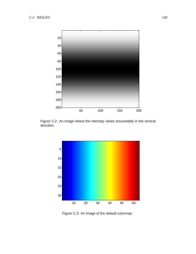
C.2. IMAGES 549
50 100 150 200
20
40
60
80
100
120
140
160
180
200
Figure C.2: An image where the intensity varies sinusoidally in the verticaldirection.
10 20 30 40 50 60
5
10
15
20
25
30
Figure C.3: An image of the default colormap.
550 APPENDIX C. LABORATORY EXERCISES
Notice that it has 64 rows and three columns. Each row is one entry in the colormap. The threecolumns give the amounts of red, green, and blue respectively in the colormap. These amounts rangefrom 0 (none of the color present) to 1.0 (the maximum amount of the color possible). Examine thecolormap to convince yourself that it begins with blue and ends with red.
Change the colormap using the colormap command as follows:
>> map = gray(256);>> colormap(map);>> image([1:256]);
Examine the map variable to understand the resulting image. This is called a grayscale colormap.
C.2.2 In-lab section
1. What is the representation in a Matlab colormap for the color white? What about black?
2. Create a � � � pixel image like that shown in figure C.2. You will want the colormapset to gray(256), as indicated above. Note that when you display this image using theimage command, it probably will not be square. This is because of the (somewhat annoying)stretching that Matlab insists on doing to make the image fit the default graphics window. Todisable the stretching and get a square image, issue the command axis image
axis image
As usual with Matlab, a brute-force way to create matrices is to use for loops, but there isalmost always a more elegant (and faster) way that exploits Matlab’s ability to operate onarrays all at once. Try to avoid using for loops to solve this and subsequent problems.
3. Change your image so that the sinusoidal variations are horizontal rather than vertical. Varythe frequency so that you get four cycles of the sinusoid instead of one. What is the frequencyof this image?
4. An image can have both vertical and horizontal frequency content at the same time. Changeyour image so that the intensity at any point is the sum of a vertical and horizontal sinusoid.Be careful to stay with the numerical range that indexes the colormap.
5. Get the image file from
http://www.eecs.berkeley.edu/˜eal/eecs20/images/helen.jpg
Save it in some directory where you have write permission with the name “helen.jpg”. (Note:For reasons that only the engineers at Microsoft could possibly explain, Microsoft InternetExplorer does not allow you to save this file as a JPEG file, ’.jpg’. It only allows you to savethe file as a bit map, ’.bmp’, which is already decoded. So we recommend using Netscaperather than IE.)
In Matlab, change the current working directory to that directory using the cd command.Then use imfinfo to get information about the file, as follows:

C.2. IMAGES 551
>> imfinfo(’helen.jpg’)
ans =
Filename: ’helen.jpg’FileModDate: ’27-Jan-2000 10:48:16’
FileSize: 18026Format: ’jpg’
FormatVersion: ’’Width: 200
Height: 300BitDepth: 24ColorType: ’truecolor’
FormatSignature: ’’
Make a note of the file size, which is given in bytes. Then use imread to read the image intoMatlab and display it as follows:
>> helen = imread(’helen.jpg’);>> image(helen);>> axis image
Use the whos command to identify the size, in bytes, and the dimensions of the helen array.Can you infer from this what is meant by ’truecolor’ above? The file is stored in JPEGformat, where JPEG, which stands for Joint Pictures Expert Group, is an image representationstandard. The imread function in Matlab decodes JPEG images. What is the compressionratio achieved by the JPEG file format (the compression ratio is defined to be size of theuncompressed data in bytes divided by the size of the compressed data in bytes).
6. The helen array returned by imread has elements that are of type uint8, which meansunsigned 8-bit integers. The possible values for such numbers are the integers from 0 to 255.The upper left pixel of the image can be accessed as follows:
>> pixel = helen(1,1,:)
pixel(:,:,1) =
205
pixel(:,:,2) =
205
552 APPENDIX C. LABORATORY EXERCISES
pixel(:,:,3) =
205
In this command, the final argument is ‘:’ which means to Matlab, return all elements in thethird dimension. The information about the result is:
>> whos pixelName Size Bytes Class
pixel 1x1x3 3 uint8 array
Grand total is 3 elements using 3 bytes
Matlab provides the squeeze command to remove dimensions of length one:
>> rgb = squeeze(pixel)
rgb =
205205205
Find the RGB values of the lower right pixel. By looking at the image, and correlating whatyou see with these RGB values, infer how white and black are represented in truecolor images.
Matlab can only do very limited operations arrays of this type.
C.2.3 Independent section
1. Construct a mathematical model for the Matlab image function as used in parts3 and 4 ofthe in-lab section by giving its domain and its range. Notice that the colormap, although itis not passed to image as an argument, is in fact an argument. It is passed in the form ofa global variable, the current colormap. Your mathematical model should show this as anexplicit argument.
2. In Matlab, you can create a movie using the following template:
numFrames = 15;m = moviein(numFrames);for frame = 1:numFrames;
... create an image X ...image(X), axis image

C.2. IMAGES 553
m(:,frame) = getframe;endmovie(m)
The line with the getframe command grabs the current image and makes it a frame of themovie. Use this template to create a vertical sinusoidal image where the sine waves appear tobe moving upwards, like waves in water viewed from above. I.e., create something like figureC.2, but where the wave appears to be moving upwards. Try help movie to learn aboutvarious ways to display this movie.
3. We can examine individually the contributions of red, green, and blue to the image by creatingcolor separations. Matlab makes this very easy on truecolor images by providing its versatilearray indexing mechanism. To extract the red portion of the helen image created above, wecan simply do:
red = helen(:,:,1);
The result is a �� � array of unsigned 8-bit integers, as we can see from the following:
>> whos redName Size Bytes Class
red 300x200 60000 uint8 array
Grand total is 60000 elements using 60000 bytes
(Note that, strangely, the squeeze command is not needed whenever the last dimension(s)collapse to size 1.) If we display this array, its value will be interepreted as indexes into thecurrent color map:
image(red), axis image
If the current colormap is the default one, then the image will look very off indeed (and verycolorful). Change the colormap to grayscale to get a more meaningful image:
map = gray(256);colormap(map);
The resulting image gives the red portion of the image, albeit rendered in black and white.Construct a colormap to render it in red. Show the Matlab code that does this in your re-port (you need not show the image). Then give similar color separations for the green andblue portions. Again, showing the Matlab code is sufficient. Hint: Create a matrix to mul-tiply pointwise by the map matrix above (using the .* operator) to zero out two of its threecolumns. The zeros and ones functions might be useful.
4. A moving average can be applied to an image, with the effect of blurring it. For simplic-ity, operate on a black and white image constructed from the above red color separation asfollows:
554 APPENDIX C. LABORATORY EXERCISES
>> bwImage = double(red);>> image(bwImage), axis image>> colormap(gray(256))
The first line converts the image to an array of doubles instead of unsigned 8-bit integersbecause Matlab cannot operate numerically on unsigned 8-bit integers. The remaining twolines simply display the image using a grayscale colormap.
Construct a new image where each pixel is the average of 25 pixels in the original image,where the 25 pixels lie in a � � � square. The new image will need to be slightly smallerthan the original (figure out why). The result should be a blurred image because the movingaverage reduces the high frequency content of a signal, and sharp edges are high frequencyphenomena.
5. A simple way to perform edge detection on a black-and-white image is to calculate the dif-ference between a pixel and the pixel immediately above it and to the left of it. If eitherdifference exceeds some threshold, we decide there is an edge at that position in the image.Perform this calculation on the image bwImage given in the previous part. To display withthe edges, start with a white image the same size or slightly smaller than the original image.When you detect an edge at a pixel, replace the white pixel with a black one. The resultingimage should resemble a line drawing of Helen. Experiment with various threshold values.Hint: To perform the threshold test, you will probably need the Matlab if command. Tryhelp if and help relop.
Note: Edge detection is often the first step in image understanding, which is the automaticinterpretation of images. A common application of image understanding is optical char-acter recognition or OCR, which is the transcription of printed documents into computerdocuments.
The difference between pixels tends to emphasize high frequency content in the image anddeemphasize low frequency content. This is why it is useful in detecting edges, which arehigh frequency content. This is obvious if we note that frequency in images refers to the rateof change of intensity over space. That rate is very fast at edges.

C.2. IMAGES 555
Instructor Verification Sheet for C.2
Name: Date:
1. Representation in a colormap of white and black.
Instructor verification:
2. Vertical sinusoidal image.
Instructor verification:
3. Horizontal higher frequency image. Give the frequency.
Instructor verification:
4. Horizontal and vertical sinusoidal image.
Instructor verification:
5. Compression ratio.
Instructor verification:
6. Representation in truecolor of white and black.
Instructor verification:
556 APPENDIX C. LABORATORY EXERCISES
C.3 State machines
State machines are sequential. They begin in a starting state, and react to a sequence of inputs bysequentially transitioning between states. Implementation of state machines in software is fairlystraightforward. In this lab, we explore doing this systematically, and build up to an implementationthat composes two state machines.
C.3.1 Background
Strings in Matlab
State machines operate on sequences of symbols from an alphabet. Sometimes, the alphabet isnumeric, but more commonly, it is a set of arbitrary elements with names that suggest their meaning.For example, the input set for the answering machine in figure3.1 is
Inputs� �ring�offhook�end greeting�end message�absent�Each element of the above set can be represented in Matlab as a string (try help strings).Strings are surrounded by single quotes. For example,
>> x = ’ring’;
The string itself is an array of characters, so you can index individual characters, as in
>> x(1:3)
ans =
rin
You can join strings just as you join ordinary arrays,
>> y = ’the’;>> z = ’bell’;>> [x, y, z]
ans =
ringthebell
However, this is not necessarily what you want. You may want instead to construct an array ofstrings, where each element of the array is a string (rather than a character). Such a collection ofstrings can be represented in Matlab as a cell array,
C.3. STATE MACHINES 557
>> c = {’ring’ ’offhook’ ’end greeting’ ’end message’ ’absent’};
Notice the curly braces instead of the usual square braces. A cell array in Matlab is an array wherethe elements of the array are arbitrary Matlab objects (such as strings and arrays). Cell arrays areindexed like ordinary arrays, so
>> c(1)
ans =
’ring’
Often, you wish to test a string to see whether it is equal to some string. You usually cannot comparestrings or cells of a cell array using ==, as illustrated here:
>> c = ’ring’;>> if (c == ’offhook’) result = 1; end??? Error using ==> ==Array dimensions must match for binary array op.
>> c = {’ring’ ’offhook’ ’end greeting’ ’end message’ ’absent’};>> if (c(1) == ’ring’) result = 1; end??? Error using ==> ==Function ’==’ not defined for variables of class ’cell’.
Strings should instead be compared using strcmp or switch (see the on-line help for thesecommands).
M-files
In Matlab, you can save programs in a file and execute them from the command line. The fileis called an m-file, and has a name of the form command.m, where commandis the name of thecommand that you enter on the command line to execute the program.
You can use any text editor to create and edit m-files, but the one built into Matlab is probably themost convenient. To invoke it, select “New” and “M-file” under the “File” menu.
To execute your program, Matlab needs to know where to find your file. The simplest way to handlethis is to make the current directory in Matlab the same as the directory storing the m-file. Forexample, if you put your file in the directory
D:\users\eal
then the following will make the file visible to Matlab

558 APPENDIX C. LABORATORY EXERCISES
>> cd D:\users\eal>> pwd
ans =
D:\users\eal
The cd command instructs Matlab to change the current working directory. The pwd commandreturns the current working directory (probably the mnemonic is presentworking directory).
You can instruct Matlab to search through some sequence of directories for your m-files, so that theydo not have to all be in the same directory. See help path. For example, instead of changingthe current directory, you could type
path(path, ’D:\users\eal’);
This command tells Matlab to search for functions wherever it was searching before (the first argu-ment path) and also in the new directory.
Suppose you create a file called hello.m containing
% HELLO - Say hello.disp(’Hello’);
The first line is a comment. The disp command displays its argument without displaying a variablename. On the command line, you can execute this
>> helloHello
Command names are not case sensitive, so HELLO is the same as Hello and hello. The commentin the file is used by Matlab to provide on-line help. Thus,
>> help hello
HELLO - Say hello.
The M-file above is a program, not a function. There is no returned value. To define a function, usethe function command in your m-file. For example, store the following in in a file reverse.m:
function result = reverse(argument)% REVERSE - return the argument array reversed.result = argument(length(argument):-1:1);

C.3. STATE MACHINES 559
Then try:
>> reverse(’hello’)
ans =
olleh
The returned value is the string argument reversed.
A function can have any number of arguments and returned values. To define a function with twoarguments, use the syntax
function [result1, result2] = myfunction(arg1, arg2)
and then assign values to result1 and result2 in the body of the file. To use such function,you must assign each of the return values to a variable as follows:
>> [r1, r2] = myfunction(a1, a2);
The names of the arguments and result variables are arbitrary.
C.3.2 In-lab section
1. Write a for loop that counts the number of occurrences of ’a’ in
>> d = {’a’ ’b’ ’a’ ’a’ ’b’};
Then define a function count that counts the number of occurrences of ’a’ in any argument.How many occurrences are there in the following two examples?
>> x = [’a’, ’b’, ’c’, ’a’, ’aa’];>> y = {’a’, ’b’, ’c’, ’a’, ’aa’};>> count(x)
ans =
??
>> count(y)
ans =
??
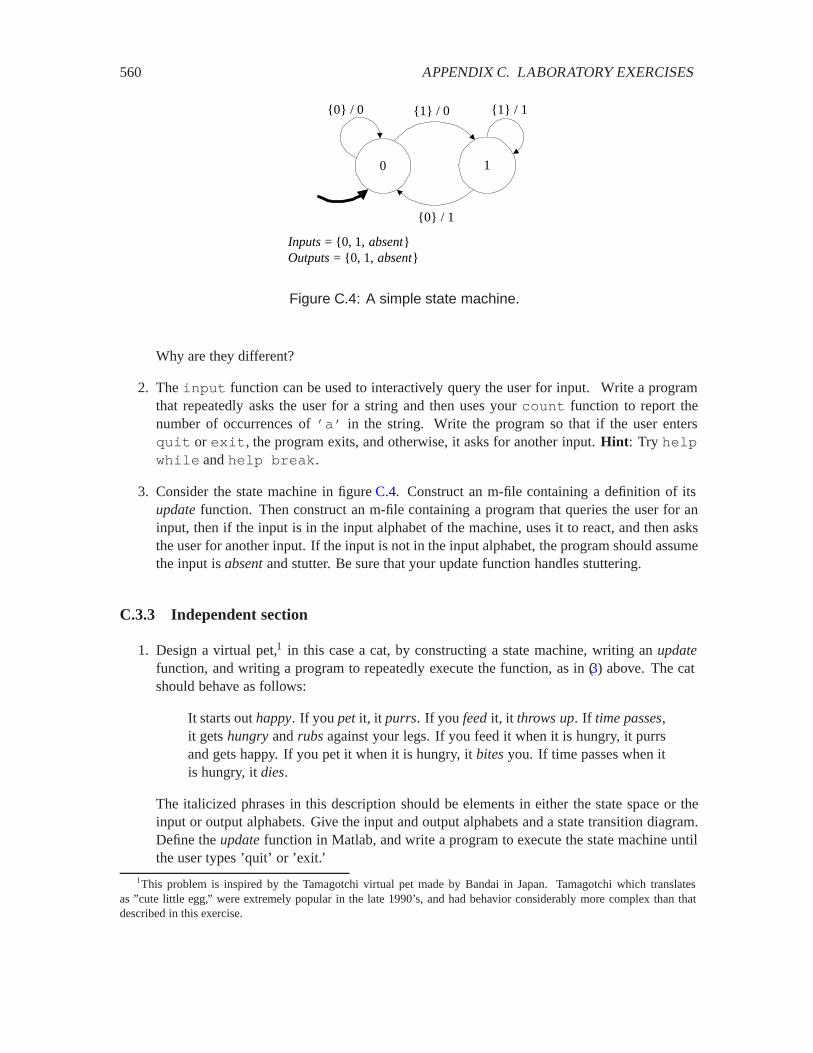
560 APPENDIX C. LABORATORY EXERCISES
0 1
{1} / 0
{0} / 1
{0} / 0 {1} / 1
Inputs = {0, 1, absent}Outputs = {0, 1, absent}
Figure C.4: A simple state machine.
Why are they different?
2. The input function can be used to interactively query the user for input. Write a programthat repeatedly asks the user for a string and then uses your count function to report thenumber of occurrences of ’a’ in the string. Write the program so that if the user entersquit or exit, the program exits, and otherwise, it asks for another input. Hint: Try helpwhile and help break.
3. Consider the state machine in figure C.4. Construct an m-file containing a definition of itsupdatefunction. Then construct an m-file containing a program that queries the user for aninput, then if the input is in the input alphabet of the machine, uses it to react, and then asksthe user for another input. If the input is not in the input alphabet, the program should assumethe input is absentand stutter. Be sure that your update function handles stuttering.
C.3.3 Independent section
1. Design a virtual pet,1 in this case a cat, by constructing a state machine, writing an updatefunction, and writing a program to repeatedly execute the function, as in (3) above. The catshould behave as follows:
It starts out happy. If you petit, it purrs. If you feedit, it throws up. If time passes,it gets hungryand rubsagainst your legs. If you feed it when it is hungry, it purrsand gets happy. If you pet it when it is hungry, it bitesyou. If time passes when itis hungry, it dies.
The italicized phrases in this description should be elements in either the state space or theinput or output alphabets. Give the input and output alphabets and a state transition diagram.Define the updatefunction in Matlab, and write a program to execute the state machine untilthe user types ’quit’ or ’exit.’
1This problem is inspired by the Tamagotchi virtual pet made by Bandai in Japan. Tamagotchi which translatesas ”cute little egg,” were extremely popular in the late 1990’s, and had behavior considerably more complex than thatdescribed in this exercise.

C.3. STATE MACHINES 561
2. Construct a state machine that provides inputs to your virtual cat so that the cat never dies.In particular, your state machine should generate time passesand feedoutputs in such a waythat the cat never reaches the diesstate.
Note that this state machine does not have particularly meaningful inputs. You can let theinput alphabet be
Inputs� ��absentwhere an input of 1 indicates that the machine should output a non-stuttering output, and aninput of absentmeans it should output a stuttering output.
Write a program where your feeder state machine is composed in cascade with your cat statemachine, and verify (experimentally) that the cat does not die. Your state machine shouldallow time to pass (by producing an infinite number of ’time passes’ outputs) but shouldotherwise be as simple as possible.
Note that a major point of this exercise is to show that systematically constructed state ma-chines can be very easily composed.
The feeder state machine is called an open-loop controller because it controls the pet withoutobserving the output of the pet. For most practical systems, it is not possible to design anopen-loop controller. The next lab explores closed-loop controllers.

562 APPENDIX C. LABORATORY EXERCISES
Instructor Verification Sheet for C.3
Name: Date:
1. Count the number of occurrences of ’a’. Understand the difference between a cell array andan array.
Instructor verification:
2. Write a program with an infinite loop and user input.
Instructor verification:
3. Construct and use updatefunction.
Instructor verification:

C.4. CONTROL SYSTEMS 563
C.4 Control systems
This lab extends the previous one by introducing nondeterminism and feedback. In particular, youwill modify the virtual pet that you constructed last time so that it behaves nondeterministically. Themodification will make it impossible to keep the pet alive by driving it with another state machinein a cascade composition. You will instead have to use a feedback composition.
This scenario is typical of a control problem. The pet is a system to be controlled, with the objectiveof keeping it alive. You will construct a controller that observes the output of the virtual pet, andbased on that output, constructs an appropriate input that will keep the pet alive. Since this controllerobserves the output of the pet, and provides input to the pet, it is called a closed-loop controller.
C.4.1 Background
Nondeterministic state machines have a possibleUpdatesfunction rather than an updatefunction.The possibleUpdatesfunction returns a set of possible updates. You will construct this function toreturn a cell array, which was explored in the previous lab.
A software implementation of a nondeterministic state machine can randomly choose from amongthe results returned by possibleUpdates. It could conceptually flip coins to determine which resultto choose each time. In software, the equivalent of coin flips is obtained through pseudo-randomnumber generators. The Matlab function rand is just such a pseudo-random number generator.The way that it works is that each time you use it, it gives you a new number (try help rand).
For this lab, you will need to be able to use cell arrays in more sophisticated ways than in theprevious lab. Recall that a cell array is like an ordinary array, except that the elements of the arraycan be arbitrary Matlab objects, including strings, arrays, or even cell arrays. A cell array can beconstructed using curly braces instead of square brackets, as in
>> letters = {’a’, ’b’, ’c’, ’d’, ’e’};>> whos lettersName Size Bytes Class
letters 1x5 470 cell array
Grand total is 10 elements using 470 bytes
The elements of the cell array can be accessed like elements of any other array, but there is onesubtlety. If you access an element in the usual way, the result is a cell array, which might not bewhat you expect. For example,
>> x = letters(2)
x =
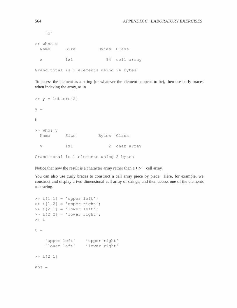
564 APPENDIX C. LABORATORY EXERCISES
’b’
>> whos xName Size Bytes Class
x 1x1 94 cell array
Grand total is 2 elements using 94 bytes
To access the element as a string (or whatever the element happens to be), then use curly braceswhen indexing the array, as in
>> y = letters{2}
y =
b
>> whos yName Size Bytes Class
y 1x1 2 char array
Grand total is 1 elements using 2 bytes
Notice that now the result is a character array rather than a � cell array.
You can also use curly braces to construct a cell array piece by piece. Here, for example, weconstruct and display a two-dimensional cell array of strings, and then access one of the elementsas a string.
>> t{1,1} = ’upper left’;>> t{1,2} = ’upper right’;>> t{2,1} = ’lower left’;>> t{2,2} = ’lower right’;>> t
t =
’upper left’ ’upper right’’lower left’ ’lower right’
>> t{2,1}
ans =
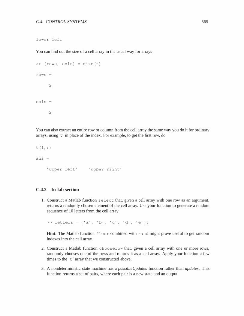
C.4. CONTROL SYSTEMS 565
lower left
You can find out the size of a cell array in the usual way for arrays
>> [rows, cols] = size(t)
rows =
2
cols =
2
You can also extract an entire row or column from the cell array the same way you do it for ordinaryarrays, using ’:’ in place of the index. For example, to get the first row, do
t(1,:)
ans =
’upper left’ ’upper right’
C.4.2 In-lab section
1. Construct a Matlab function select that, given a cell array with one row as an argument,returns a randomly chosen element of the cell array. Use your function to generate a randomsequence of 10 letters from the cell array
>> letters = {’a’, ’b’, ’c’, ’d’, ’e’};
Hint: The Matlab function floor combined with rand might prove useful to get randomindexes into the cell array.
2. Construct a Matlab function chooserow that, given a cell array with one or more rows,randomly chooses one of the rows and returns it as a cell array. Apply your function a fewtimes to the ’t’ array that we constructed above.
3. A nondeterministic state machine has a possibleUpdatesfunction rather than updates. Thisfunction returns a set of pairs, where each pair is a new state and an output.

566 APPENDIX C. LABORATORY EXERCISES
A convenient Matlab implementation is a function that returns a two-dimensional cell array,with each of the possible updates on one row. As a first step towards this, modify yourrealization of the updatefunction for the virtual cat of the previous lab so that it returns a � � cell array with the next state and output. Also modify your program that runs the cat(without the driver) so that it uses your new function. Verify that the cat still works properly.
4. Now modify the cat’s behavior so that if it is hungry and you feed it, it sometimes gets happyand purrs (as it did before), but it sometimes stays hungry and rubs against your legs. I.e.,change your updatefunction so that if the state is hungry and you feed the cat, then return a�� � cell array where the two rows specify the two possible next state, output pairs. Modifythe program that runs the cat to use your chooserow function to choose from among theoptions.
5. Compose your driver machine from the previous lab with your nondeterministic cat, andverify that the driver no longer keeps the cat alive. In fact, no open-loop controller will beable to keep the cat alive and allow time to pass. In the independent section of this lab, youwill construct a closed-loop controller that keeps the cat alive. It is a feedback compositionof state machines.
C.4.3 Independent section
Design a deterministic state machine that you can put into a feedback composition with your non-deterministic cat so that the cat is kept alive and time passes. Give the state transition diagram foryour state machine and write a Matlab function that implements its updatefunction. Write a Matlabprogram that implements the feedback composition.
Note that your program that implements the feedback composition faces a challenging problem.When the program starts, neither the inputs to the controller machine nor the inputs to the catmachine are available. So neither machine can react. For your controller machine, you shoulddefine Matlab functions for both update, which requires a known input, and output, which doesnot. The output function, given the current state, returns the output that will be produced by thenext reaction, if it is known, or unknownif it is not known. In the case of your controller, it shouldalways be known, or the feedback composition will not be well formed.
Verify (by running your program) that the cat does not die.

C.4. CONTROL SYSTEMS 567
Instructor Verification Sheet for C.4
Name: Date:
1. Generated random sequence of letters using ’select’.
Instructor verification:
2. Applied chooserow to the ’t’ array.
Instructor verification:
3. The cat still works with the update function returning a cell array.
Instructor verification:
4. The nondeterministic sometimes stays hungry when fed.
Instructor verification:
5. The nondeterministic cat dies under open-loop control.
Instructor verification:
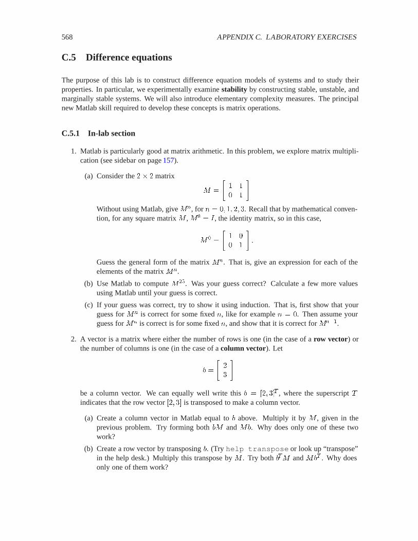
568 APPENDIX C. LABORATORY EXERCISES
C.5 Difference equations
The purpose of this lab is to construct difference equation models of systems and to study theirproperties. In particular, we experimentally examine stability by constructing stable, unstable, andmarginally stable systems. We will also introduce elementary complexity measures. The principalnew Matlab skill required to develop these concepts is matrix operations.
C.5.1 In-lab section
1. Matlab is particularly good at matrix arithmetic. In this problem, we explore matrix multipli-cation (see sidebar on page 157).
(a) Consider the �� � matrix
3 �
�
Without using Matlab, give 3�, for � � � � �� �. Recall that by mathematical conven-tion, for any square matrix 3 , 3� � � , the identity matrix, so in this case,
3� �
��
Guess the general form of the matrix 3�. That is, give an expression for each of theelements of the matrix 3�.
(b) Use Matlab to compute 3��. Was your guess correct? Calculate a few more valuesusing Matlab until your guess is correct.
(c) If your guess was correct, try to show it using induction. That is, first show that yourguess for 3� is correct for some fixed �, like for example � � . Then assume yourguess for 3� is correct is for some fixed �, and show that it is correct for 3���.
2. A vector is a matrix where either the number of rows is one (in the case of a row vector) orthe number of columns is one (in the case of a column vector). Let
� �
��
�
be a column vector. We can equally well write this � � ��� ��� , where the superscript indicates that the row vector ��� �� is transposed to make a column vector.
(a) Create a column vector in Matlab equal to � above. Multiply it by 3 , given in theprevious problem. Try forming both �3 and 3�. Why does only one of these twowork?
(b) Create a row vector by transposing �. (Try help transpose or look up “transpose”in the help desk.) Multiply this transpose by 3 . Try both ��3 and 3�� . Why doesonly one of them work?
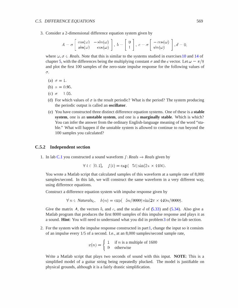
C.5. DIFFERENCE EQUATIONS 569
3. Consider a 2-dimensional difference equation system given by
� � @
������ � ������������ ������
�� � �
�� ! � @
� ������������
�� � � �
where �� @ Reals. Note that this is similar to the systems studied in exercises10 and 14 ofchapter 5, with the differences being the multiplying constant @ and the ! vector. Let � � ���and plot the first 100 samples of the zero-state impulse response for the following values of@.
(a) @ � .
(b) @ � ���.
(c) @ � ��.
(d) For which values of @ is the result periodic? What is the period? The system producingthe periodic output is called an oscillator.
(e) You have constructed three distinct difference equation systems. One of these is a stablesystem, one is an unstable system, and one is a marginally stable. Which is which?You can infer the answer from the ordinary English-language meaning of the word “sta-ble.” What will happen if the unstable system is allowed to continue to run beyond the100 samples you calculated?
C.5.2 Independent section
1. In lab C.1 you constructed a sound waveform � �Reals� Realsgiven by
� �� �� ��� � )$*���� ������ � ����
You wrote a Matlab script that calculated samples of this waveform at a sample rate of 8,000samples/second. In this lab, we will construct the same waveform in a very different way,using difference equations.
Construct a difference equation system with impulse response given by
� � Naturals�� ���� � )$*������� ������ � �������
Give the matrix �, the vectors �, and !, and the scalar � of (5.33) and (5.34). Also give aMatlab program that produces the first 8000 samples of this impulse response and plays it asa sound. Hint: You will need to understand what you did in problem3 of the in-lab section.
2. For the system with the impulse response constructed in part1, change the input so it consistsof an impulse every 1/5 of a second. I.e., at an 8,000 samples/second sample rate,
���� �
� if � is a multiple of 1600 otherwise
Write a Matlab script that plays two seconds of sound with this input. NOTE: This is asimplified model of a guitar string being repeatedly plucked. The model is justifiable onphysical grounds, although it is a fairly drastic simplification.

570 APPENDIX C. LABORATORY EXERCISES
3. Compare the complexity of the state machine model and the one you constructed in labC.1.In particular, assuming in each case that you generate one second of sound at an 8,000 sam-ples/second sample rate, count the number of scalar multiplications and additions that mustbe done to construct the sound vector. In the realization in labC.1, you used the built-in Mat-lab functions exp and sin. These functions are surprisingly expensive to compute, so counteach evaluation of exp or sin on a scalar argument as 20 multiplications and 15 additions(they are actually typically more expensive even than this). You should find that the statemachine realization is far less expensive by this measure. Do not count the cost of the Matlabsound function, which we can’t easily determine.
C.5. DIFFERENCE EQUATIONS 571
Instructor Verification Sheet for C.5
Name: Date:
1. Matrix multiplication in Matlab, and induction demonstration.
Instructor verification:
2. Matrix-vector multiplication.
Instructor verification:
3. Sinusoids with exponential envelopes; stability.
Instructor verification:

572 APPENDIX C. LABORATORY EXERCISES
C.6 Differential equations
The purpose of this lab is to experiment with models of continuous-time systems that are describedas differential equations. The exercises aim to solidify state-space concepts while giving someexperience with software that models continuous-time systems.
The lab uses Simulink, a companion to Matlab. The lab is self contained, in the sense that noadditional documentation for Simulink is needed. Instead, we rely on the on-line help facilities. Bewarned, however, that these are not as good for Simulink as for Matlab. The lab exercise will guideyou, trying to steer clear of the more confusing parts of Simulink.
Simulink is a block-diagram modeling environment. As such, it has a more declarative flavor thanMatlab, which is imperative. You do not specify exactly how signals are computed in Simulink. Yousimply connect together blocks that represent systems. These blocks declare a relationship betweenthe input signal and the output signal.
Simulink excels at modeling continuous-time systems. Of course, continuous-time systems are notdirectly realizable on a computer, so Simulink must simulate the system. There is quite a bit ofsophistication in how this is done. The fact that you do not specify how it is done underscores theobservation that Simulink has a declarative flavor.
The simulation is carried out by a solver, which examines the block diagram you have specifiedand constructs an execution that simulates its behavior. As you read the documentation and interactwith the software, you will see various references to the solver. In fact, Simulink provides a varietyof solvers, and many of these have parameters you can control. Indeed, simulation of continuous-time systems is generally inexact, and some solvers work better on some models than others. Themodels that we will construct work well with the default solver, so we need not be concerned withthis (considerable) complication.
Simulink can also model discrete-time systems, and (a bit clumsily) mixed discrete and continuous-time systems. We will emphasize the continuous-time modeling because this cannot be done (con-veniently) in Matlab, and it is really the strong suit of Simulink.
C.6.1 Background
To run Simulink, start Matlab and type simulink at the command prompt. This will open theSimulink library browser. To explore Simulink demos, at the Matlab command prompt, type demo,and then find the Simulink item in the list that appears. To get an orientation about Simulink, openthe help desk (using the Help menu), and find Simulink. Much of what is in the help desk will notbe very useful to you. Find a section with a title “Building a Simple Model” or something similarand read that.
We will build models in state-space form, as in chapter 5, and as in the previous lab, but in con-tinuous time. A continuous-time state-space model for a linear system has the form (see section5.4)
���� � ���� � �"�� (C.1)

C.6. DIFFERENTIAL EQUATIONS 573
/�� � !��� � �"�� (C.2)
where
� ��Reals� Reals� gives the state response;
� ���� is the derivative of � evaluated at Reals;
� "�Reals� Realsis the input signal; and
� /�Reals� Realsis the output signal.
The input and output are scalars, so the models are SISO , but the state is a vector of dimension � ,which in general can be larger than one. The derivative of a vector � is simply the vector consistingof the derivative of each element of the vector.
The principle that we will follow in modeling such a system is to use an Integrator block, whichlooks like this in Simulink:
s
1
Integrator
This block can be found in the library browser under “Simulink” and “Continuous.” Create a newmodel by clicking on the blank-document icon at the upper left of the library browser, and drag anintegrator into it. You should see the same icon as above.
If the input to the integrator is ��, then the output is � (just think about what happens when youintegrate a derivative). Thus, the pattern we will follow is to provide as the input to this block asignal ��.
We begin with a one-dimensional system (� � ) in order to get familiar with Simulink. Considerthe scalar differential equation
���� � ���� (C.3)
where � Realsis a given scalar and ��Reals� Realsand ��� is some given initial state. Wewill set things up so that the input to the integrator is �� and the output is �. To provide the input,however, we need the output, since ���� � ����. So we need to construct a feedback system thatlooks like this:
s
1
Integrator
1
Gain
This model seems self-referential, and in fact it is, just as is (C.3).
Construct the above model. You can find the triangular “Gain” block in the library browser under“Simulink” and “Math.” To connect the blocks, simply place the cursor on an output port and clickand drag to an input port.
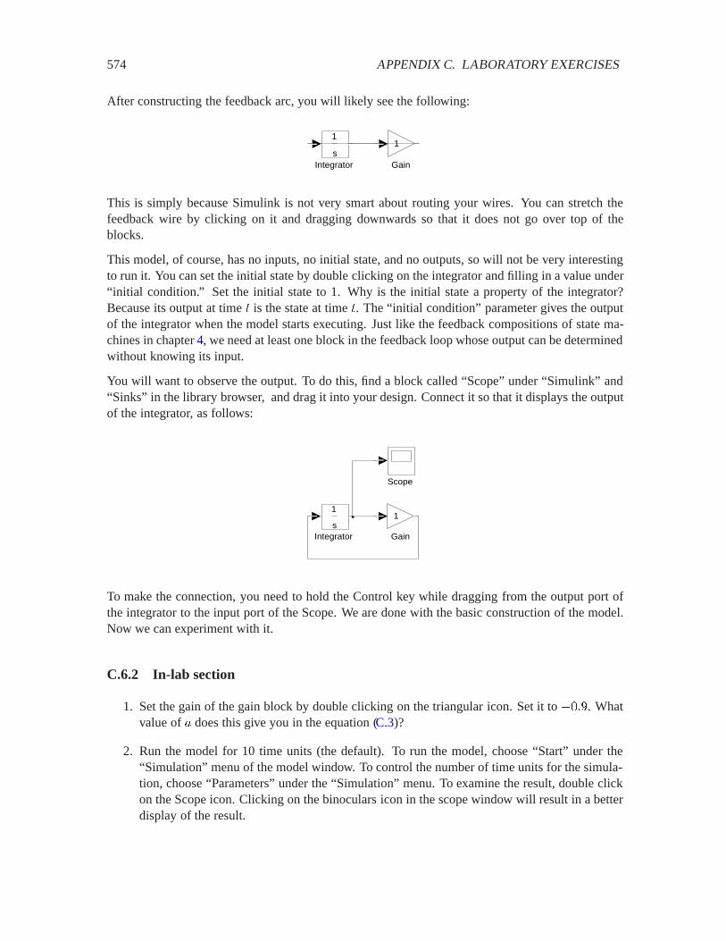
574 APPENDIX C. LABORATORY EXERCISES
After constructing the feedback arc, you will likely see the following:
s
1
Integrator
1
Gain
This is simply because Simulink is not very smart about routing your wires. You can stretch thefeedback wire by clicking on it and dragging downwards so that it does not go over top of theblocks.
This model, of course, has no inputs, no initial state, and no outputs, so will not be very interestingto run it. You can set the initial state by double clicking on the integrator and filling in a value under“initial condition.” Set the initial state to 1. Why is the initial state a property of the integrator?Because its output at time is the state at time . The “initial condition” parameter gives the outputof the integrator when the model starts executing. Just like the feedback compositions of state ma-chines in chapter 4, we need at least one block in the feedback loop whose output can be determinedwithout knowing its input.
You will want to observe the output. To do this, find a block called “Scope” under “Simulink” and“Sinks” in the library browser, and drag it into your design. Connect it so that it displays the outputof the integrator, as follows:
Scope
s
1
Integrator
1
Gain
To make the connection, you need to hold the Control key while dragging from the output port ofthe integrator to the input port of the Scope. We are done with the basic construction of the model.Now we can experiment with it.
C.6.2 In-lab section
1. Set the gain of the gain block by double clicking on the triangular icon. Set it to ���. Whatvalue of � does this give you in the equation (C.3)?
2. Run the model for 10 time units (the default). To run the model, choose “Start” under the“Simulation” menu of the model window. To control the number of time units for the simula-tion, choose “Parameters” under the “Simulation” menu. To examine the result, double clickon the Scope icon. Clicking on the binoculars icon in the scope window will result in a betterdisplay of the result.

C.6. DIFFERENTIAL EQUATIONS 575
3. Write down analytically the function � given by this model. You can guess its form by exam-ining the simulation result. Verify that it satisfies (C.3) by differentiating.
4. Change the gain block to have value �� instead of��� and re-run the model. What happens?Is the system stable? (Stable means that if the input is bounded for all time, then the outputis bounded for all time. In this case, clearly the input is bounded since it is zero.) Give ananalytical formula for � for this model.
5. Experiment with values of the gain parameter. Determine over what range of values thesystem is stable.
C.6.3 Independent section
Continuous-time linear state-space models are reasonable for some musical instruments. In thisexercise, we will simulate an idealized and a more realistic tuning fork, which is a particularlysimple instrument to model. The model will be two-dimensional continuous-time state-space model.
Consider the state and output equations (C.1) and (C.2). Since the model is two dimensional, thestate at each time is now a two-dimensional vector. The “initial condition” parameter of the Inte-grator block in Simulink can be given a vector. Set the initial value to the column vector
��� �
�� (C.4)
The factor � must be a � � � matrix if the state is a two dimensional column vector. Unfortu-nately, the Gain block in Simulink cannot be given a matrix parameter. You must replace the Gainblock with the MatrixGain block, also found in the “Math” library under “Simulink” in the librarybrowser.
At first, we will assume there is no input, and we will examine the state response. Thus, we are onlyconcerned at first with the simplified state equation
���� � ����� (C.5)
Recall that in chapter 2, equation (2.11) states that the displacement ��� at time of a tine of thetuning fork satisfies the differential equation
���� � �������where �� is constant that depends on the mass and stiffness of the tine, and and where ���� denotesthe second derivative with respect to time of � (see box on page57). This does not have the form of(C.5). However, we can put it in that form using a simple trick. Let
��� �
�������
�
and observe that
���� �
��������
��
576 APPENDIX C. LABORATORY EXERCISES
Thus, we can write (C.5) as
���� �
��������
��
���� �������� ����
� �������
�
for suitably chosen constants ����, ����, ����, and ����.
1. Find ����, ����, ����, and ���� for the tuning fork model.
2. Use Simulink to plot the state response of the tuning fork when the initial state is given by(C.4). You will have to pick a value of ��. Use Simulink to help you find a value of �� sothat the state completes one cycle in 10 time units. Each sample of the state response has twoelements. These represent the displacement and speed, respectively, of the tuning fork tine inthe model. The displacement is what directly translates into sound.
3. Change �� so that the state has a frequency of 440 Hz, assuming the time units are seconds.Change the simulation parameters so that you run the model through 5 complete cycles.
4. Change the simulation parameters so that you run the model through 1 second. Use theSimulink To Workspace block to write the result to the workspace, and then use the Matlabsoundsc function to listen to it. Note: You will need to set the sample time parameter of theTo Workspace block to 1/8000. You will also need to specify that the save format should be amatrix. For your lab report, print your block diagram and annotate it with all the parametersthat have values different from the defaults.
5. In practice, a tuning fork will not oscillate forever as the model does. We can add dampingby modifying the matrix �. Try replacing the zero value of ���� with �. What happens tothe sound? This is called damping. Experiment with different values for ����. Describe howthe different values affect the sound. Determine (experimentally) for what values of ���� thesystem is stable.
6. A tuning fork is not much of a musical instrument. Its sound is too pure (spectrally). Aguitar string, however, operates on similar principles as the tuning fork, but has a much moreappealing sound.
A tuning fork vibrates with only one mode. A guitar string, however, vibrates with multiplemodes, as illustrated in figure C.5. Each of these vibrations produces a different frequency.The top one in the figure produces the lowest frequency, called the fundamental, which istypically the frequency of the note being played, such as 440 Hz for A-440. The next modeproduces a component of the sound at twice that frequency, 880 Hz; this component is calledthe first harmonic. The third produces three times the frequency, 1320 Hz, and the fourthproduces four times the fundamental, 1760 Hz; these components are the second and thirdharmonics.
If the guitar string is undamped, and the fundamental frequency is �� Hz, then the the com-bined sound is a linear combination of the fundamental and the three (or more) harmonics.This can be written as a continuous-time function � where for all Reals,
��� ���
���
!��&�������

C.6. DIFFERENTIAL EQUATIONS 577
Figure C.5: Four modes of vibration of a guitar string.
where � is the number of harmonics and !� gives the relative weights of these harmonics.The values of !� will depend on the guitar construction and how it is played, and affect thetimbre of the sound.
The model you have constructed above generates a damped sinusoid at 440 Hz. Create aSimulink model that produces a fundamental of 440 Hz plus three harmonics. Experimentwith the amplitudes of the harmonics relative to the fundamental, as well as with the ratesof decay of the four components. Note how the quality of the sound changes. Your reportshould include a printout of your model with the parameter values that you have chosen toget a sound like that of a plucked string.

578 APPENDIX C. LABORATORY EXERCISES
Instructor Verification Sheet for C.6
Name: Date:
1. Value of �.
Instructor verification:
2. Plot of the state response.
Instructor verification:
3. Formula for function �. Verified by differentiating.
Instructor verification:
4. Formula for function �.
Instructor verification:
5. Range of values for the gain over which the system is stable.
Instructor verification:

C.7. SPECTRUM 579
C.7 Spectrum
The purpose of this lab is to learn to examine the frequency domain content of signals. Two methodswill be used. The first method will be to plot the discrete Fourier series coefficients of finite signals.The second will be to plot the Fourier series coefficients of finite segments of time-varying signals,creating what is known as a spectrogram.
C.7.1 Background
A finite discrete-time signal with ( samples has a discrete-time Fourier series expansion
���� � �� �
#���������
�� ����6���� <�� (C.6)
for ( odd and
���� � �� �
#������
�� ����6���� <�� (C.7)
for ( even, where �� � ���(.
A finite signal can be considered to be one cycle of a periodic signal with fundamental frequency��, in units of radians per sample, or �( in Hertz. In this lab, we will assume ( is always even,and we will plot the magnitude of each of the frequency components, ����� � ��#��� for each ofseveral signals, in order to gain intuition about the meaning of these coefficients.
Notice that each ���� gives the amplitude of the sinusoidal component of the signal at frequency6�� � 6���(, which has units of radians per sample. In order to interpret these coefficients, youwill probably want to convert these units to Hertz. If the sampling frequency is �� samples persecond, then you can do the conversion as follows (see box on page221):
�6���(��radians/sample����samples/second����radians/cycle�
� 6���(�cycles/second�
Thus, each ���� gives the amplitude of the sinusoidal component of the signal at frequency 6���(Hz.
Note that Matlab does not have any built-in function that directly computes the discrete Fourierseries coefficients. However, it does have a realization of the fast Fourier transform, a functioncalled fft, which can be used to construct the Fourier series coefficients. In particular, fouri-erSeries is a function that returns the DFS coefficients2:
function [magnitude, phase] = fourierSeries(x)% FOURIERSERIES - Return the magnitude and phase of each% sinusoidal component in the Fourier series expansion for
2This function can be found at http://www.eecs.berkeley.edu/ eal/eecs20/matlab/fourierSeries.m.
580 APPENDIX C. LABORATORY EXERCISES
% the argument, which is interpreted as one cycle of a% periodic signal. The argument is assumed to have an% even number p of samples. The first returned value is an% array containing the amplitudes of the sinusoidal% components in the Fourier series expansion, with% frequencies 0, 1/p, 2/p, ... 1/2. The second returned% value is an array of phases for the sinusoidal% components. Both returned values are arrays with length% (p/2)+1.p = length(x);f = fft(x)/p;magnitude(1) = abs(f(1));upper = p/2;magnitude(2:upper) = 2*abs(f(2:upper));magnitude(upper+1) = abs(f(upper+1));phase(1) = angle(f(1));phase(2:upper) = angle(f(2:upper));phase(upper+1) = angle(f(upper+1));
In particular, if you have an array x with even length,
[A, phi] = fourierSeries(x);
returns the DFS coefficients in a pair of vectors.
To plot the magnitudes of the Fourier series coefficients vs. frequency, you can simply say
p = length(x);frequencies = [0:fs/p:fs/2];plot(frequencies, A);xlabel(’frequency in Hertz’);ylabel(’amplitude’);
where fs has been set to the sampling frequency (in samples per second). The line
frequencies = [0:fs/p:fs/2];
bears further examination. It produces a vector with the same length as A, namely � (��, where (is the length of the x vector. The elements of the vector are the frequencies in Hertz of each Fourierseries component.
C.7.2 In-lab section
1. To get started, consider the signal generated by
C.7. SPECTRUM 581
t = [0:1/8000:1-1/8000];x = sin(2*pi*800*t);
This is 8000 samples of an 800 Hz sinusoid sampled at 8,000 samples/second. Listen to it.Use the fourierSeries function as described above to plot the magnitude of its discreteFourier series coefficients. Explain the plot.
Consider the continuous-time sinusoid
��� � ���������
The x vector calculated above is 8000 samples of this sinusoid taken at a sample rate of 8kHz. Notice that the frequency of the sinusoid is the derivative of the argument to the sinefunction,
� ��
���� � ���
in units of radians per second. This fact will be useful below when looking at more interestingsignals.
2. With t as above, consider the more interesting waveform generated by
y = sin(2*pi*800*(t.*t));
This is called a chirp. Listen to it. Plot its Fourier series coefficients using the fouri-erSeries function as described above.
This chirp is 8 kHz samples of the continuous-time waveform
��� � ����������
The instantaneous frequency of this waveform is defined to be the derivative of the argumentto the sine function,
��� ��
����� � ����
For the given values t used to compute samples y, what is the range of instantaneous fre-quencies? Explain how this corresponds with the plot of the Fourier series coefficients, andhow it corresponds with what you hear.
3. The Fourier series coefficients computed in part 2 describe the range of instantaneous fre-quencies of the chirp pretty well, but they do not describe the dynamics very well. Plot theFourier series coefficients for the waveform given by
z = y(8000:-1:1);
Listen to this sound. Does it sound the same as y? Does its Fourier series plot look the same?Why?
582 APPENDIX C. LABORATORY EXERCISES
4. The chirp signal has a dynamically varying frequency-domain structure. More precisely, thereare certain properties of the signal that change slowly enough that our ears detect them as achange in the frequency structure of the signal rather than as part of the frequency structure(the timbre or tonal content). Recall that our ears do not hear sounds below about 30 Hz.Instead, the human brain hears changes below 30 Hz as variations in the nature of the soundrather than as frequency domain content. The Fourier series methods used above fail to reflectthis psychoacoustic phenomenon.
A simple fix is the short-time Fourier series. The chirp signals above have 8000 samples,lasting one second. But since we don’t hear variations below 30 Hz as frequency content, itprobably makes sense to reanalyze the chirp signal for frequency content 30 times in the onesecond. This can be done using the following function:3
function waterfallSpectrogram(s, fs, sizeofspectra, numofspectra)
% WATERFALLSPECTROGRAM - Display a 3-D plot of a spectrogram% of the signal s.%% Arguments:% s - The signal.% fs - The sampling frequency (in samples per second).% sizeofspectra - The number of samples to use to calculate each% spectrum.% numofspectra - The number of spectra to calculate.
frequencies = [0:fs/sizeofspectra:fs/2];offset = floor((length(s)-sizeofspectra)/numofspectra);for i=0:(numofspectra-1)
start = i*offset;[A, phi] = fourierSeries(s((1+start):(start+sizeofspectra)));magnitude(:,(i+1)) = A’;
endwaterfall(frequencies, 0:(numofspectra-1), magnitude’);xlabel(’frequency’);ylabel(’time’);zlabel(’magnitude’);
To invoke this function on the chirp, do
t = [0:1/8000:1-1/8000];y = sin(2*pi*800*(t.*t));waterfallSpectrogram(y, 8000, 400, 30);
which yields the plot shown in figure C.6. That plot shows 30 distinct sets of Fourier seriescoefficients, each calculated using 400 of the 8000 available samples. Explain how this plotdescribes the sound you hear. Create a similar plot for the reverse chirp, signal z given in part3.
3This code can be found at http://www.eecs.berkeley.edu/ eal/eecs20/matlab/waterfallSpectrogram.m.
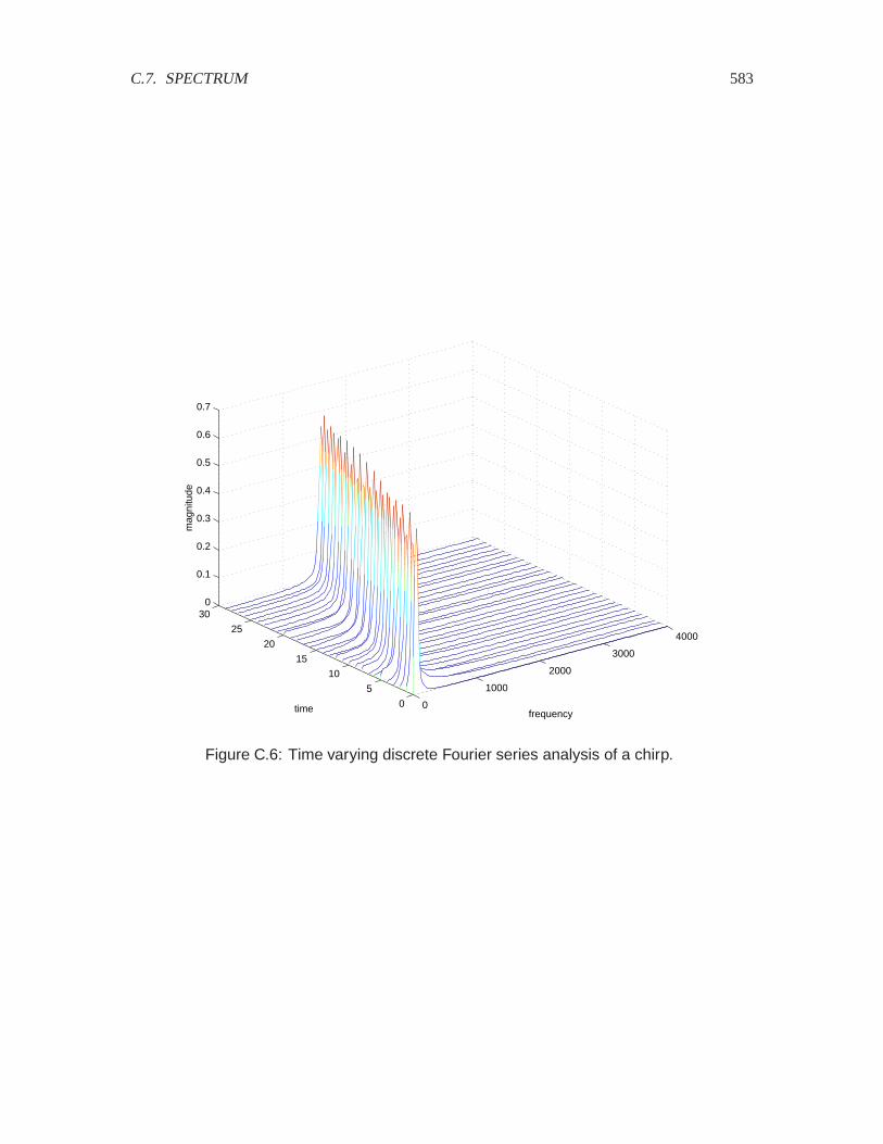
C.7. SPECTRUM 583
0
1000
2000
3000
4000
0
5
10
15
20
25
300
0.1
0.2
0.3
0.4
0.5
0.6
0.7
frequencytime
mag
nitu
de
Figure C.6: Time varying discrete Fourier series analysis of a chirp.
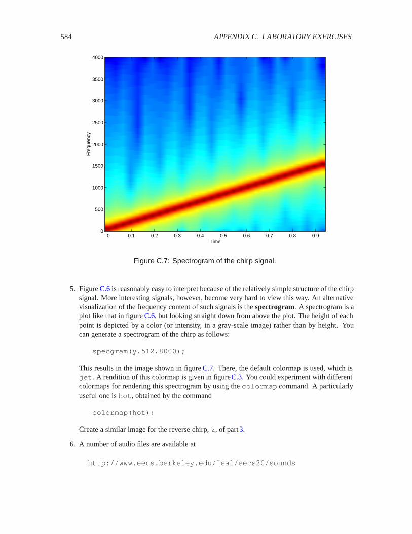
584 APPENDIX C. LABORATORY EXERCISES
Time
Fre
quen
cy
0 0.1 0.2 0.3 0.4 0.5 0.6 0.7 0.8 0.90
500
1000
1500
2000
2500
3000
3500
4000
Figure C.7: Spectrogram of the chirp signal.
5. Figure C.6 is reasonably easy to interpret because of the relatively simple structure of the chirpsignal. More interesting signals, however, become very hard to view this way. An alternativevisualization of the frequency content of such signals is the spectrogram. A spectrogram is aplot like that in figure C.6, but looking straight down from above the plot. The height of eachpoint is depicted by a color (or intensity, in a gray-scale image) rather than by height. Youcan generate a spectrogram of the chirp as follows:
specgram(y,512,8000);
This results in the image shown in figure C.7. There, the default colormap is used, which isjet. A rendition of this colormap is given in figureC.3. You could experiment with differentcolormaps for rendering this spectrogram by using the colormap command. A particularlyuseful one is hot, obtained by the command
colormap(hot);
Create a similar image for the reverse chirp, z, of part 3.
6. A number of audio files are available at
http://www.eecs.berkeley.edu/˜eal/eecs20/sounds
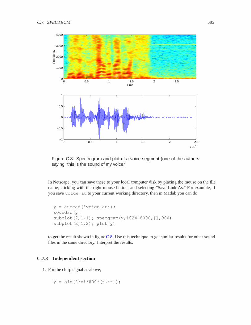
C.7. SPECTRUM 585
Time
Fre
quen
cy
0 0.5 1 1.5 2 2.50
1000
2000
3000
4000
0 0.5 1 1.5 2 2.5
x 104
−1
−0.5
0
0.5
1
Figure C.8: Spectrogram and plot of a voice segment (one of the authorssaying “this is the sound of my voice.”
In Netscape, you can save these to your local computer disk by placing the mouse on the filename, clicking with the right mouse button, and selecting ”Save Link As.” For example, ifyou save voice.au to your current working directory, then in Matlab you can do
y = auread(’voice.au’);soundsc(y)subplot(2,1,1); specgram(y,1024,8000,[],900)subplot(2,1,2); plot(y)
to get the result shown in figure C.8. Use this technique to get similar results for other soundfiles in the same directory. Interpret the results.
C.7.3 Independent section
1. For the chirp signal as above,
y = sin(2*pi*800*(t.*t));
586 APPENDIX C. LABORATORY EXERCISES
generate the discrete Fourier series coefficients using fourierSeries as explained in sec-tion C.7.1. Then, write a Matlab function that uses (C.7) to reconstruct the original signalfrom the coefficients. Your Matlab function should begin as follows:
function x = reconstruct(magnitude, phase)% RECONSTRUCT - Given a vector of magnitudes and a vector% of phases, construct a signal that has these magnitudes% and phases as its discrete Fourier series coefficients.% The arguments are assumed to have odd length, p/2 + 1,% and the returned vector will have length p.
Note that this function will require a large number of computations. If your computer is notup to the task, the construct the Fourier series coefficients for the first 1000 samples instead ofall 8000, and reconstruct the original from those coefficients. To check that the reconstructionworks, subtract your reconstructed signal from y and examine the difference. The differencewill not be perfectly zero, but it should be very small compared to the original signal. Plotthe difference signal.
2. In the remainder of this lab, we will study beat signals, which are combinations of sinusoidalsignals with closely spaced frequencies. First, we need to develop some background.
Use Euler’s relation to show that
� ������� ������� � ������� � ���� � ������� � �����
for any ��, ��, and in Reals. Hint: See box on page 263.
A consequence of this identity is that if two sinusoidal signals with different frequencies, ��and ��, are multiplied together, the result is the same as if two sinusoids with two otherfrequencies, �� � �� and �� � ��, are added together.
3. Construct the sum of two cosine waves with frequencies of 790 and 810 Hz. Assume thesample rate is 8 kHz, and construct a vector in Matlab with 8000 samples. Listen to it.Describe what you hear. Plot the first 800 samples (1/10 second). Explain how the plotillustrates what you hear. Explain how the identity in part2 explains the plot.
4. What is the period of the waveform in part 3? What is the fundamental frequency for itsFourier series expansion? Plot its discrete Fourier series coefficients (the magnitude only)using fourierSeries. Plot its spectrogram using specgram. Choose the parametersof specgram so that the warble is clearly visible. Which of these two plots best reflectsperception?

C.7. SPECTRUM 587
Instructor Verification Sheet for C.7
Name: Date:
1. Plot of the DFS coefficients of the sinusoid, with explanation.
Instructor verification:
2. Plot of the DFS, plus range of instantaneous frequencies, plus correspondence with the sound.
Instructor verification:
3. Plot of the DFS is the same, yet the sound is different. Explanation.
Instructor verification:
4. Explain how figure C.6 describes the sound you hear. Plot the reverse chirp.
Instructor verification:
5. Create and interpret a spectrogram for one other sound file, at least.
Instructor verification:

588 APPENDIX C. LABORATORY EXERCISES
C.8 Comb filters
The purpose of this lab is to use a kind of filter called a comb filter to deeply explore concepts ofimpulse response and frequency response.
The lab uses Simulink, like lab C.6. Unlike lab C.6, it will use Simulink for discrete-time processing.Be warned that discrete-time processing is not the best part of Simulink, so some operations will beawkward. Moreover, the blocks in the block libraries that support discrete-time processing are notwell organized. It can be difficult to discover how to do something as simple as an � -sample delayor an impulse source. We will identify the blocks you will need.
The lab is self contained, in the sense that no additional documentation for Simulink is needed. Asin lab C.6, be warned that the on-line documentation is not as good for Simulink as for Matlab. Youwill want to follow our instructions closely, or you are likely to discover very puzzling behavior.
C.8.1 Background
To run Simulink, start Matlab and type simulink at the command prompt. This will open theSimulink library browser. The library browser is a hierarchical listing of libraries with blocks. Thenames of the libraries are (usually) suggestive of the contents, although sometimes blocks are foundin surprising places, and some of the libraries have meaningless names (such as “Simulink”).
Here, we explain some of the techniques you will need to implement the lab. You may wish to skimthese now and return them when you need them.
Simulation Parameters
First, since we will be processing audio signals with a sample rate of 8,000 samples per second, youneed to force Simulink to execute the model as a discrete-time model with sample rate 8,000 samplesper second (recall that Simulink excels at continuous-time modeling). Open a blank model byclicking on the document icon at the upper left of the library browser window. Find the Simulationmenu in that window, and select Parameters. Set the parameters so that the window looks likewhat is shown in figure C.9. Specifically, set the stop time to 4.0 (seconds), the solver options to“Fixed-step” and “discrete (no continuous states),” and the fixed step size to 1/8000.
Reading and Writing Audio Signals
Surprisingly, Simulink is more limited and awkward than Matlab in its ability to read and writeaudio files. Consequently, the following will seem like more trouble than it is worth. Bear withus. Simulink only supports Microsoft wave files, which typically have the suffix “.wav”. You mayobtain a suitable audio file for this lab at
http://www.eecs.berkeley.edu/˜eal/eecs20/sounds/voice.wav
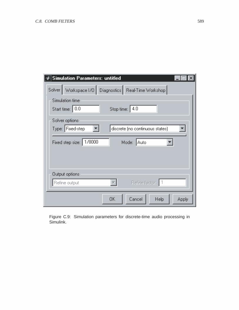
C.8. COMB FILTERS 589
Figure C.9: Simulation parameters for discrete-time audio processing inSimulink.

590 APPENDIX C. LABORATORY EXERCISES
simout
To Workspace
From Wave Filevoice
(8000Hz/1Ch/8b)
From WaveFile
Figure C.10: Test model for Simulink audio.
In Netscape you can go to
http://www.eecs.berkeley.edu/˜eal/eecs20/sounds/
and then right click on the voice.wav filename to bring up a menu, and choose “Save Link As...”to save the file to your local disk. It is best to then, in the Matlab command window, to change thecurrent working directory to the one in which you stored the file using the cd command. This willmake it easier to use the file.
To make sure we can process audio signals, create the test model shown in figureC.10. To do this,in a new model window with the simulation parameters set as explained in “Simulation Parameters”on page 588, create an instance of the block called From Wave File. This block can be found inthe library browser under DSP Blockset and DSP Sources. Set the parameters of that blockto
File name: voice.wavSamples per frame: 1
The first parameter assumes you have set the current working directory to the directory containingthe voice.wav file. The second indicates to Simulink that it should produce audio samples one ata time, rather than collecting them into vectors to produce many at once.
Next, find the To Workspace block in the Simulink block library, under Sinks. Create an instanceof that block in your model. Edit its parameters to change the “Save format” to “Array” (or “Matrix,”depending on your Matlab version). You can leave other parameters at their default values.
Connect the blocks as shown in figure C.10.
Assuming the simulation parameters have been set as explained in “Simulation Parameters” on page588, you can now run the model by invoking the Start command under the Simulation menu. Thiswill result in a new variable called simout appearing in the Matlab workspace. In the Matlabcommand window, do
soundsc(simout)
to listen to the voice signal.
Note that the DSP Sinks library has a block called To Wave Device, which in theory willproduce audio directly to the audio device. In practice, however, it seems much easier to use the To
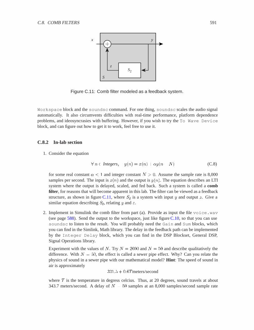
C.8. COMB FILTERS 591
S2
S
x y
z
Figure C.11: Comb filter modeled as a feedback system.
Workspace block and the soundsc command. For one thing, soundsc scales the audio signalautomatically. It also circumvents difficulties with real-time performance, platform dependenceproblems, and ideosyncrasies with buffering. However, if you wish to try the To Wave Deviceblock, and can figure out how to get it to work, feel free to use it.
C.8.2 In-lab section
1. Consider the equation
� � Integers� ���� � ���� � *������ (C.8)
for some real constant * ) and integer constant � 2 . Assume the sample rate is 8,000samples per second. The input is ���� and the output is ����. The equation describes an LTIsystem where the output is delayed, scaled, and fed back. Such a system is called a combfilter, for reasons that will become apparent in this lab. The filter can be viewed as a feedbackstructure, as shown in figure C.11, where .� is a system with input � and output �. Give asimilar equation describing .�, relating � and �.
2. Implement in Simulink the comb filter from part (a). Provide as input the file voice.wav(see page 588). Send the output to the workspace, just like figure C.10, so that you can usesoundsc to listen to the result. You will probably need the Gain and Sum blocks, whichyou can find in the Simlink, Math library. The delay in the feedback path can be implementedby the Integer Delay block, which you can find in the DSP Blockset, General DSP,Signal Operations library.
Experiment with the values of � . Try � � � and � � � and describe qualitatively thedifference. With � � �, the effect is called a sewer pipe effect. Why? Can you relate thephysics of sound in a sewer pipe with our mathematical model? Hint: The speed of sound inair is approximately
���� � � meters/second
where is the temperature in degress celcius. Thus, at 20 degrees, sound travels at about343.7 meters/second. A delay of � � � samples at an 8,000 samples/second sample rate

592 APPENDIX C. LABORATORY EXERCISES
is equal to the time it takes sound to travel roughly 2 meters, twice the diameter of a 1 metersewer pipe.
Experiment with the value of *. What happens when * � ? What happens when * � ?When * 2 ? You may wish to plot the output in addition to listening to it.
3. Modify your Simulink model so that its output is the first one second (the first 8001 samples)of the impulse response of the system defined by (C.8), with * � ��� and � � �.
The simplest approach is to provide an impulse as an input. To do that, use the DiscretePulse Generator block, found in the Simulink, Sources. This block can be (sort of)configured to generate a Kronecker delta function. Set its amplitude to 1, its period tosomething longer than the total number of samples (i.e. larger than 8001), its pulse width to1, its phase delay to 0, and its sample time to 1/8000.
You will also want to change the simulation parameters to execute your system for 1 secondinstead of 4.
Listen to the impulse response. Plot it. Can you identify the tone that you hear? Is it a musicalnote? Hint: Over short intervals, a small fraction of a second, the impulse response is roughlyperiodic. What is its period?
4. In the next lab you will modify the comb filter to generate excellent musical sounds resem-bling plucked strings, such as guitars. As a first step towards that goal, we can make a muchless mechanical sound than the impulse response by initializing the delay with random data.Modify your Simulink model so that the comb filter has no input, and instead of an input, theInteger Delay block is given random initial conditions. Use * � ��� and � � �, andchange the parameters of the Integer Delay block so that its initial conditions are givenby
randn(1,40)
The Matlab randn function returns a vector of random numbers (try help randn in theMatlab command window).
Listen to the result. Compare it to the sound of the impulse response. It should be richer,and less mechanical, but should have the same tone. It is also louder (even though soundscscales the sound).
C.8.3 Independent section
The comb filter is an LTI system. Figure C.11 is a special case of the feedback system consideredin section 8.5.2, which is shown there to be LTI. Thus, if the input is
���� � ����
then the output is���� � ;�������

C.8. COMB FILTERS 593
where ;�Reals� Complexis the frequency response. Find the frequency response of the combfilter. Plot the magnitude of the frequency response over the range 0 to 4 kHz using Matlab. Whyis it called a comb filter? Explain the connection between the tone that you hear and the frequencyresponse.

594 APPENDIX C. LABORATORY EXERCISES
Instructor Verification Sheet for C.8
Name: Date:
1. Found an equation for .�, relating � and �.
Instructor verification:
2. Constructed Simulink model and obtained both sewer pipe effect and echo effect.
Instructor verification:
3. Constructed the impulse response and identified the tone.
Instructor verification:
4. Created sound with random values in the feedback delay.
Instructor verification:
C.9. PLUCKED STRING INSTRUMENT 595
C.9 Plucked string instrument
The purpose of this lab is to experiment with models of a plucked string instrument, using it todeeply explore concepts of impulse response, frequency response, and spectrograms. The methodsdiscussed in this lab were invented by Karplus and Strong, and first reported in
K. Karplus and A. Strong, “Digital Sythesis of Plucked-String and Drum Timbres,”Computer Music Journal, vol. 7, no. 2, pp. 43-55, Summer 1983.
The lab uses Simulink, like lab C.8. It assumes you have understood that lab and the techniques ituses in detail.
C.9.1 Background
In the previous lab, you constructed in Simulink the feedback system shown in figureC.11, where.� was an � sample delay. In this lab, you will enhance the model by replacing .� with slightlymore complicated filters. These filters will consist of the same � sample delay in cascade with twoother filters, a lowpass filter and an allpass filter. The objective will be to get truly high-qualityplucked string sounds.
Delays
Recall from example 8.9 that the � sample delay system has frequency response
;��� � ����� �
This same frequency response was obtained in example9.10 by calculating the DTFT of the impulseresponse. Note that the magnitude response is particularly simple,
�;���� � �
Recall that this is an allpass filter.
The phase response is� ;��� � ����
The phase response is a linear function of frequency, �, with slope �� . A filter with such a phaseresponse is said to have linear phase. A delay is particularly simple form of a linear phase filter.Notice that the amount of delay is the negative of the derivative of the phase response,
�� ;���
��� ���
This fact will be useful when we consider more complicated filters than this simple delay.
596 APPENDIX C. LABORATORY EXERCISES
Allpass Filters
We will need a slightly more complicated allpass filter than the � sample delay. Consider a filtergiven by the following difference equation,
� � Integers� ���� � ����� � � ����� � ���� � (C.9)
for some constant ) � � . This defines an LTI system, so if the input is ���� � ����, then theoutput is ;�������, where ; is the frequency response. We can determine the frequency responseusing this fact by plugging this input and output into (C.9),
;������� � �;������ ���� � ����� � ��� �����
This can be rewritten as
;�������� � ������ � ������� ������
Eliminating ���� on both sides we get
;���� � ������ � �� �����
Solving for ;��� we get
;��� ��� ����
� ������ (C.10)
We could immediately proceed to plotting the magnitude and phase response using Matlab, butinstead, we will first manipulate this further to get some insight. Being slightly tricky, we willmultiply top and bottom by ����� to get
;��� ������� � ������
����� � ��������
Now notice that the top and bottom are complex conjugates of one another. I.e., let
���� � ������ � ������ (C.11)
and note that
;��� �����
������
Since the numerator and denominator have the same magnitude,4
�;���� � �
The filter is allpass!
The phase response, however, is more complicated. Note that
� ;��� � � ����� � ������
4 For any two complex numbers / and ), note that /�) � /�) and � �/�)� � � �/�� � �)�.
C.9. PLUCKED STRING INSTRUMENT 597
But since for any complex number �, � ���� � �� ���,
� ;��� � �� �����
Thus, to find the phase response, we simply need to find � ����. Plugging Euler’s relation into(C.11) we get
���� � ��� � �������� � &��� � ���������
Since the angle of a complex number � is ������Im���Re���,
� ;��� � � ��������� � ��������
��� � ��������
��
Since ����/� � ����/�� ����/�,
� ;��� � � ��������
�� ��������
��
This form yields insight for small �. In particular, when � is small (compared to �),
�������� � ����
so� ;��� � � �����
���
�� ���
��
Since ) � � , the argument to the arctangent is small if � is small, so for low frequencies,
� ;��� � ��
�� � � ����
where � is defined by
� � ���
�� � (C.12)
Thus, at low frequencies, this allpass filter has linear phase with slope ��. At low frequencies,therefore, it is an allpass with linear phase, which means that behave exactly like a delay! However,unlike the � sample delay, the amount of delay is �, which depending on � can be any real numberbetween 0 and 1. Thus, this allpass filter gives us a way to get fractional sample delays in a discretetime system, at least at low frequencies.
C.9.2 In-lab section
1. The lowpass filter we will use is a simple, length two moving average. If the input is � andthe output is �, then the filter is given by the difference equation,
� � Integers� ���� � ������� � ���� ��� (C.13)
Find an expression for the frequency response of the lowpass filter given by (C.13). Use Mat-lab to plot the magnitude and phase response over the frequency range 0 to � radians/sample.Is this a linear phase filter? If so, what is its delay?

598 APPENDIX C. LABORATORY EXERCISES
2. In part 4 of the previous lab, you initialized a comb filter with random noise and produceda sound that reasonably well approximates a plucked string instrument, such as a guitar. Wecan improve the sound.
Real instrument sounds have more dynamics in their frequency structure. That is, the spec-trum of the sound within the first few milliseconds of plucking the string is different from thespectrum a second or so later. Physically, this is because the high frequency vibrations of thestring die out more rapidly than the low frequency vibrations.
We can approximate this effect by modifying the comb filter by inserting the lowpass filtergiven by (C.13) into the feedback loop. This can be accomplished by realizing the followingdifference equation:
� � Integers� ���� � ���� � ��*���� ��� � ����� � ���
Modify your Simulink model you constructed in part 4 of the previous lab so that it usesa lowpass filter in the feedback loop, implementing this difference equation. Listen to theresulting sound, and compare it against the sound from the previous lab. Use * � ��� and� � �, as before. Can you hear the improvement?
3. In the last lab, you found that the tone of the sound generated by the comb filter had frequency��� , where � was the delay in the feedback loop, and 8000 was the sampling frequency.You used � � � to get a fundamental frequency of 200 Hz. Now, you have added anadditional lowpass filter, which introduces additional delay in the feedback loop. You havedetermined that additional delay in part 1 above. What is the fundamental frequency now?
The comb filter delay can only delay by an integer number of samples. The lowpass filterintroduces a fixed delay. Consequently, there are only certain fundamental frequencies thatare possible. In particular, assuming the sample rate is 8,000 samples/second, is it possibleto achieve a fundamental frequency of 440 Hz? This would be essential to have a reasonableguitar model, since we would certainly want to be able to play the note A-440 on the guitar.Determine the closest achievable frequency to 440 Hz. Is it close enough? In the independentsection of this lab, you will show how to achieve a fundamental frequency very close to 440Hz.
C.9.3 Independent section
1. Show analytically that the lowpass filter given by (C.13) has linear phase over the range offrequencies 0 to � radians/sample, and determine the slope. Verify that this agrees with theplot you constructed in the In-Lab section.
2. In part 2 of the in-lab section, you combined an � -sample delay with a lowpass filter in thefeedback path of a comb filter. Calculate the frequency response of this version of the combfilter, and plot its magnitude using Matlab over the frequency range 0 to �. Compare it to thefrequency response you calculated for the original comb filter in the previous lab. Find thefundamental frequency of the musical note from this plot and compare it to the answer thatyou gave in part 3 of the in-lab portion. Hint: The spectral peaks are very sharp, so you willneed to calculate the magnitude frequency at many points in the range 0 to � to be sure to hitthe peaks. We recommend calculating at least 2000 points.

C.9. PLUCKED STRING INSTRUMENT 599
3. The reason that the comb filter with a lowpass filter in the feedback loop yields a muchbetter plucked string sound than the comb filter by itself is that it more accurately modelsthe physical phenomenon that higher frequency vibrations on the string die out faster thanlower frequency vibrations. Plot the spectrogram using specgram of the generated soundto demonstrate this phenomenon, and explain how your spectrogram demonstrates it.
4. Verify that the frequency response (C.10) of the allpass filter has constant magnitude andlinear phase for low frequencies by plotting it using Matlab. Plot it for the following values ofdelay: � � �� ��� ��� ����. Plot it over the range of frequencies 0 to � radians/sample.Discuss how your plots support the conclusions about this filter. Hint: Use (C.12) to find �given �.
5. You determined in part 3 of the in-lab section that you could not get very close to A-440 witha comb filter with a lowpass filter in the feedback loop. The allpass filter given by (C.10),however, can be used to achieve delays that are a fraction of a sample period. Implement theallpass filter, modifying your Karplus-Strong plucked string model by putting the allpass filterin the feedback loop. Set the parameters of the allpass filter and � to get an A-440. Showyour Simulink diagram, and give the parameters of all the blocks.

600 APPENDIX C. LABORATORY EXERCISES
Instructor Verification Sheet for C.9
Name: Date:
1. Magnitude and phase of lowpass filter. Linear phase? Delay?
Instructor verification:
2. Improved plucked string sound.
Instructor verification:
3. Fundamental frequencies that are possible.
Instructor verification:
C.10. MODULATION AND DEMODULATION 601
C.10 Modulation and demodulation
The purpose of this lab is to learn to use frequency domain concepts in practical applications. Theapplication selected here is amplitude modulation (AM), a widely used technique in communi-cation systems, including of course AM radio, but also almost all digital communication systems,including digital cellular telephones, voiceband data modems, and wireless networking devices. Asecondary purpose of this lab is to gain a working knowledge of the fast Fourier transform (FFT)algorithm, and an introductory working knowledge of filter design. Note that this lab requires theSignal Processing Toolbox of Matlab for filter design.
C.10.1 Background
Amplitude Modulation
The problem addressed by AM modulation is that we wish to convey a signal from one point inphysical space to another through some channel. The channel has certain constraints, and in partic-ular, can typically only pass frequencies within a certain range. An AM radio station, for example,might be constrained by government regulators to broadcast only radio signals in the range of 720kHz to 760 kHz, a bandwidth of 40 kHz.
The problem, of course, is that the radio station has no interest in broadcasting signals that onlycontain frequencies in the range 720 kHz to 760 kHz. They are more likely to want to transmit avoice signal, for example, which contains frequencies in the range of about 50 Hz to about 10 kHz.AM modulation deals with this mismatch by modulating the voice signal so that it is shifted to theappropriate frequency range. A radio receiver, of course, must demodulate the signal, since 720kHz is well above the hearing range of humans.
In this lab, we present a somewhat artificial scenario in order to maximize the experience. We willkeep all frequencies that we work with within the audio range so that you can listen to any signal.Therefore, we will not modulate a signal up to 720 kHz (you would not be able to hear the result).Instead, we present the following scenario:
Assume we have a signal that contains frequencies in the range of about 100 to 300 Hz,and we have a channel that can pass frequencies from 700 to 1300 Hz.5 Our task willbe to modulate the first signal so that it lies entirely within the channel passband, andthen to demodulate to recover the original signal.
AM modulation is studied in detail in exercise16 of chapter 10. In that problem, you showed that if
��� � ��� ��������
then the CTFT is$ ��� � ��� � ����� ���� � ������
5Since Fourier transforms of real signals are symmetric, the signal also contains frequencies in the range -100 to -300Hz, and the channel passes frequencies in the range -700 to -1300 Hz.

602 APPENDIX C. LABORATORY EXERCISES
In this lab, we will get a similar result experimentally, but working entirely with discrete-timesignals, and staying entirely within the audio range so that we can hear (and not just plot) theresults.
The FFT Algorithm
In order to understand AM modulation, we need to be able to calculate and examine Fourier trans-forms. We will do this numerically in this lab, unlike exercise 16 of chapter 10, where it is doneanalytically.
In lab C.7, we used a supplied function called fourierSeries to calculate the Fourier seriescoefficients �� and <� for signals. In this lab, we will use the built-in function fft, which is used, infact, by the fourierSeries function. Learning to use the FFT is extremely valuable; it is widelyused all analytical fields that involve time series analysis, including not just all of engineering, butalso the natural sciences and social sciences. The FFT is also widely abused by practitioners whodo not really understand what it does.
The FFT algorithm operates most efficiently on finite signals whose lengths are a power of 2. Thus,in this lab, we will work with what might seem like a peculiar signal length, 8192. This is ���. Atan 8,000 samples/second sample rate, it corresponds to slightly more than one second of sound.
Recall that a periodic discrete-time signal with period ( has a discrete-time Fourier series expansion
���� � �� �
#���������
�� ����6���� <�� (C.14)
for ( odd and
���� � �� �
#������
�� ����6���� <�� (C.15)
for ( even, where �� � ���(, the fundamental frequency in cycles per sample. Recall further thatwe can alternatively write the Fourier series expansion in terms of complex exponentials,
���� �#�
���
��������� (C.16)
Note that this sum covers one cycle of the periodic signal. If what we have is a finite signal insteadof a periodic signal, then we can interpret the finite signal as being one cycle of a periodic signal.
In chapter 10, we describe four Fourier transforms. The only one of these that is computable on acomputer is the DFT, or discrete Fourier transform. For a periodic discrete-time signal � withperiod (, we have the inverse DFT, which takes us from the frequency domain to the time domain,
� � Integers� ���� �
(
#������
� ���
������ (C.17)
C.10. MODULATION AND DEMODULATION 603
and the DFT, which takes us from the time domain to the frequency domain,
� 6 Integers� ��� �
#������
��'�������� � (C.18)
Comparing (C.17) and (C.16), we see that the DFT yields coefficients that are just scaled versionsof the Fourier series coefficients. This scaling is conventional.
In lab C.7 we calculated �� and <�. In this lab, we will calculate ���. This can be done using
(C.18). The FFT algorithm is simply a computationally efficient algorithm for calculating (C.18).
In Matlab, you will collect 8192 samples of a signal into a vector and then invoke the fft function.Invoke help fft to verify that this function is the right one to use. If your 8192 samples are in avector x, then fft(x)will return a vector with 8192 complex number, representing ��� ���� ����� .
From (C.18) it is easy to verify that �� � ���# for all integers 6 (see part 1 of the in-lab sectionbelow). Thus, the DFT � is a periodic, discrete function with period (. If you have the vectorfft(x), representing ��� ��������� , you know all ��. For example,
��� � �������� � �����
From C.17, you can see that each �� scales a complex exponential component at frequency 6�� �6���(, which has units of samples per second. In order to interpret the DFT coefficients ��, youwill probably want to convert the frequency units to Hertz. If the sampling frequency is �� samplesper second, then you can do the conversion as follows (see box on page221):
�6���(��radians/sample����samples/second����radians/cycle�
� 6���(�cycles/second� (C.19)
Thus, each �� gives the DFT value at frequency 6���( Hz. For our choices of numbers, �� � �and ( � ���, so �� gives the DFT value at frequency 6 � ��� Hz.
Filtering in Matlab
The filter function can compute the output of an LTI system given by a difference equation ofthe form
������ � ��������������� �����������������������������3��� (C.20)
To find the output �, first collect the (finite) signal � into a vector. Then collect the coefficients��� � �� into a vector A of length � , and the coefficients ��� � �� into a vector B of length 3 .Then just do
y = filter(B, A, x);
Example 3.1: Consider the difference equation
���� � ����� ������ � ��

604 APPENDIX C. LABORATORY EXERCISES
0 10 20 30 40 50 60 70 80 90 100−1
−0.8
−0.6
−0.4
−0.2
0
0.2
0.4
0.6
0.8
1
Figure C.12: Impulse response of a simple filter.
We can find and plot the first 100 samples of the impulse response by letting the vector� be an impulse and using filter to calculate the output:
x = [1, zeros(1,99)];y = filter([1], [1, 0.95], x);stem(y);
which yields the plot shown in C.12. The natural question that arises next is how todecide on the values of B and A. This is addressed next.
Filter Design in Matlab
The signal processing toolbox of Matlab provides a set of useful functions that return filter coeffi-cients A and B given a specification of a desired frequency response. For example, suppose we havea signal sampled at 8 kHz and we wish to design a filter that passes all frequency components below1 kHz and removes all frequency components above that. The following Matlab command designsa filter that approximates this specification:
[B, A] = butter(10, 0.25);
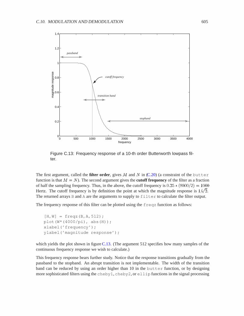
C.10. MODULATION AND DEMODULATION 605
0 500 1000 1500 2000 2500 3000 3500 40000
0.2
0.4
0.6
0.8
1
1.2
1.4
frequency
mag
nitu
de r
espo
nse
cutoff frequency
stopband
transition band
passband
Figure C.13: Frequency response of a 10-th order Butterworth lowpass fil-ter.
The first argument, called the filter order, gives 3 and � in (C.20) (a constraint of the butterfunction is that 3 � � ). The second argument gives the cutoff frequency of the filter as a fractionof half the sampling frequency. Thus, in the above, the cutoff frequency is ��� � ����� � Hertz. The cutoff frequency is by definition the point at which the magnitude response is �
��.
The returned arrays B and A are the arguments to supply to filter to calculate the filter output.
The frequency response of this filter can be plotted using the freqz function as follows:
[H,W] = freqz(B,A,512);plot(W*(4000/pi), abs(H));xlabel(’frequency’);ylabel(’magnitude response’);
which yields the plot shown in figure C.13. (The argument 512 specifies how many samples of thecontinuous frequency response we wish to calculate.)
This frequency response bears further study. Notice that the response transitions gradually from thepassband to the stopband. An abrupt transition is not implementable. The width of the transitionband can be reduced by using an order higher than 10 in the butter function, or by designingmore sophisticated filters using the cheby1, cheby2, or ellip functions in the signal processing
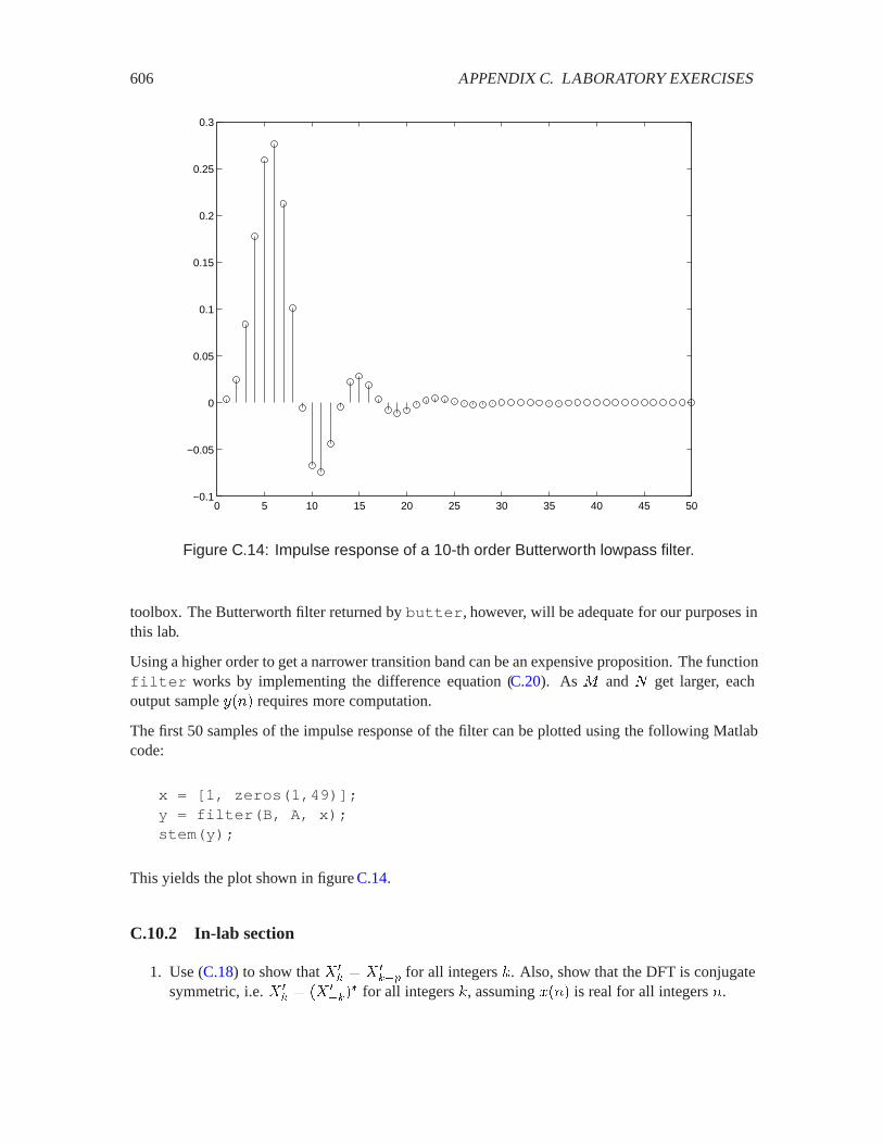
606 APPENDIX C. LABORATORY EXERCISES
0 5 10 15 20 25 30 35 40 45 50−0.1
−0.05
0
0.05
0.1
0.15
0.2
0.25
0.3
Figure C.14: Impulse response of a 10-th order Butterworth lowpass filter.
toolbox. The Butterworth filter returned by butter, however, will be adequate for our purposes inthis lab.
Using a higher order to get a narrower transition band can be an expensive proposition. The functionfilter works by implementing the difference equation (C.20). As 3 and � get larger, eachoutput sample ���� requires more computation.
The first 50 samples of the impulse response of the filter can be plotted using the following Matlabcode:
x = [1, zeros(1,49)];y = filter(B, A, x);stem(y);
This yields the plot shown in figure C.14.
C.10.2 In-lab section
1. Use (C.18) to show that ��� � � �
��# for all integers 6. Also, show that the DFT is conjugatesymmetric, i.e. ��
� � �� ����
� for all integers 6, assuming ���� is real for all integers �.

C.10. MODULATION AND DEMODULATION 607
2. In part 2 of the in-lab portion of lab C.7, we studied a chirp signal. We will use a similarsignal here, although it will vary over a narrower range of frequencies. Construct the signal xgiven by:
t = [0:1/8000:8191/8000];x = sin(2*pi*100*t + 2*pi*100*(t.*t));
This is a chirp that varies from about 100 Hz to about 300 Hz. Listen to it. Calculate its DFTusing the fft function, and plot the magnitude of the DFT. Construct your plot in such a waythat your horizontal axis is labeled in Hertz, not in the index 6 of ��. The horizontal axisshould vary in frequency from 0 to 8000 Hz.
3. Your plot from part 2 should show frequency components in the range 100 Hz to 300 Hz, butin addition, it shows frequency components in the range 7700 to 7900. These extra compo-nents are the potentially the most confusing aspect of the DFT, but in fact, they are completelypredictable from the mathematical properties of the DFT.
Recall that the DFT of a real signal is conjugate symmetric. Thus,
�� ��� � �� �
����Thus, if there are frequency components in the range 100 to 300 Hz, then there should alsobe frequency components with the same magnitude in the range -100 to -300 Hz. These donot show up on your plot simply because you have not plotted the frequency components atnegative frequencies.
Recall that the DFT is periodic with period (. That is, �� � ���# for all integers 6. Recallfrom (C.19) that the 6 � � DFT coefficient represents a frequency component at 6���(Hertz, where �� is the sampling frequency, 8000 Hertz. Thus, a frequency component atsome frequency � must be identical to a frequency component at � � ��. Therefore, thecomponents in the range -100 to -300 Hertz must be identical to the components in the range7700 to 7900 Hertz! The image we are seeing in that latter range is a consequence of theconjugate symmetry and periodicity of the DFT!
Since the DFT is periodic with period 8000 Hertz (when using units of Hertz), it possiblymakes more sense to plot its values in the range -4000 to 4000 Hertz, rather than 0 to 8000Hertz. This way, we can see the symmetry. Since the DFT gives the weights of complexexponential components, the symmetry is intuitive, because it takes two complex exponentialswith frequencies that are negatives of one another to yield a real-valued sinusoid.
Manipulate the result of the fft function to yield a plot of the DFT of the chirp where thehorizontal axis is -4000 to 4000 Hertz. It is not essential to include both endpoints, at -4000and at 4000 Hertz, since they are constrained to be identical anyway by periodicity.
C.10.3 Independent section
1. For the chirp signal as above, multiply it by a sine wave with frequency 1 kHz, and plot themagnitude of the DFT of the result over the frequency range -4000 to 4000 Hz. Verify thatthe resulting signal will get through the channel described in the scenario on page601. Listento the modulated chirp. Does what you hear correspond with what you see in the DFT plot?

608 APPENDIX C. LABORATORY EXERCISES
2. The modulated chirp signal constructed in the previous part can be demodulated by multiply-ing it again by a sine wave with frequency 1 kHz. Form that product, and plot the magnitudeof the DFT of the result over the frequency range -4000 to 4000 Hz. How does the resultdiffer from the original chirp? Listen to the resulting signal. Would this be an acceptabledemodulation by itself?
3. Use the butter function to design a filter that will process the result of the previous part sothat it more closely resembles the original signal. You should be able to get very close with amodest filter order (say, 5). Filter the result of the previous part, listen to the result, and plotthe magnitude of its DFT in the frequency range -4000 to 4000 Hz.
The modulation and demodulation method you have just implemented is similar to what isused many communication systems. A number of practical problems have to be overcome inpractice, however. For example, the receiver usually does not know the exact frequency andphase of the carrier signal, and hence it has to somehow infer this frequency and phase fromthe signal itself. One technique is to simply include the carrier in the modulated signal byadding it in. Instead of transmitting
��� � ��� ��������
we can transmit��� � � � ���� ��������
in which case, the transmitted signal will contain the carrier itself. This can be used fordemodulation. Another technique is to construct a phase locked loop, a clever device thatextracts the carrier from the transmitted signal without it being explicitly present. This methodis used in digital transmission schemes. The details, however, must be left to a more advancedtext.
In the scheme we have just implemented, the amplitude of a carrier wave is modulated tocarry a signal. It turns out that we can also vary the phase of the carrier to carry additionalinformation. Such AM-PM methods are used extensively in digital transmission. Thesemethods make more efficient use of precious radio bandwidth than AM alone.
C.10. MODULATION AND DEMODULATION 609
Instructor Verification Sheet for C.10
Name: Date:
1. Verify periodicity and conjugate symmetry of the DFT.
Instructor verification:
2. Plot of the magnitude of the DFT, correctly labeled, from 0 to 8000 Hz.
Instructor verification:
3. Plot of the magnitude of the DFT, correctly labeled, from -4000 to 4000 Hz.
Instructor verification:
610 APPENDIX C. LABORATORY EXERCISES
C.11 Sampling and aliasing
The purpose of this lab is to study the relationship between discrete-time and continuous-timesignals by examining sampling and aliasing. Of course, a computer cannot directly deal withcontinuous-time signals. So instead, we will construct discrete-time signals that are defined assamples of continuous-time signals, and then operate entirely on them, downsampling them to getnew signals with lower sample rates, and upsampling them to get signals with higher sample rates.
Note that this lab has no independent part. Therefore, no lab writeup needs to be turned in. Theinstructor verification sheet is sufficient.
C.11.1 In-lab section
1. Recall from lab C.7 that a chirp signal given by
��� � ���������
has instantaneous frequency�
����� � ���
in radians per second, or��
in Hertz. A sampled signal � � Sampler� ��� with sampling interval will be
���� � ��������� ����
Create in Matlab a chirp sampled at 8,000 samples/second that lasts 10 seconds and sweepsfrom frequency 0 to 12 kHz. Listen to the chirp. Explain the aliasing artifacts that you hear.
2. For the remainder of this lab, we will work with a particular chirp signal that has a convenientFourier transform for visualizing and hearing aliasing effects. For efficient computation usingthe FFT algorithm, we will work with ��� � ��� samples, giving slightly more than 1 secondof sound at an 8,000 samples/second sample rate. You may wish to review labC.10, whichexplains how to create well-labeled plots of the DFT of a finite signal using the FFT algorithm.
The chirp signal we wish to create is given by
� �� ��� ��� � ��� ���������
where � is the duration of the signal and ��� is a time-varying amplitude given by
��� � � �������������This chirp starts with amplitude 0, rising linearly to peak at the midpoint of the duration, andthen falls again back to zero, as shown in figureC.15. Thus, it has a triangular envelope.
Generate such a chirp that lasts for 8192 samples at an 8 kHz sample rate and sweeps from afrequency of zero to 2500 Hz. Listen to the resulting sound. Are there any aliasing artifacts?Why or why not?
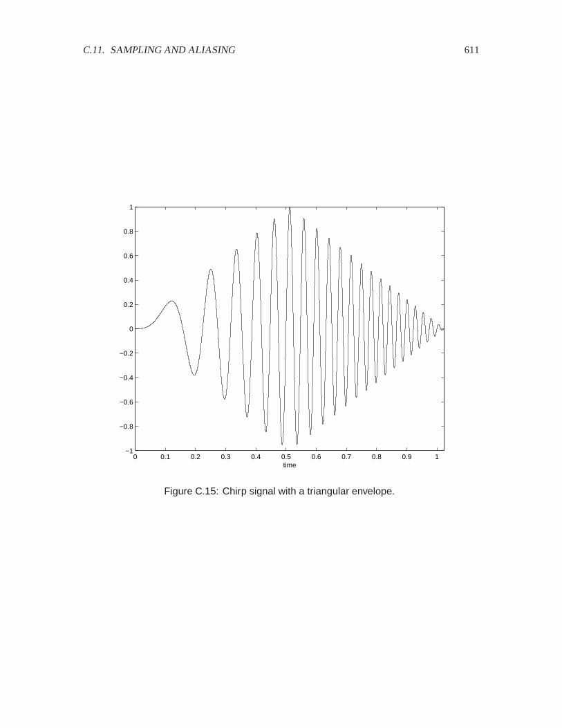
C.11. SAMPLING AND ALIASING 611
0 0.1 0.2 0.3 0.4 0.5 0.6 0.7 0.8 0.9 1−1
−0.8
−0.6
−0.4
−0.2
0
0.2
0.4
0.6
0.8
1
time
Figure C.15: Chirp signal with a triangular envelope.

612 APPENDIX C. LABORATORY EXERCISES
3. Use the FFT algorithm, as done in lab C.10, to create a plot of the magnitude of the DFTof the chirp signal from the previous part over the frequency range �� kHz to 4 kHz. Makesure the horizontal axis of your plot is labeled in Hertz. Does your plot look like a sensiblefrequency-domain representation of this chirp?
4. Modify your chirp so that it sweeps from 0 to 5 kHz. Listen to it. Do you hear aliasingartifacts? Plot the magnitude of the DFT over �� kHz to 4 kHz. Can you see the aliasingartifacts in this plot? Explain why the plot has the shape that it does.
5. Return to the chirp that you generated in part 2, which sweeps from 0 to 2500 Hz. Createa new signal with sample rate 4,000 samples/second by downsampling that chirp. That is,create a vector in Matlab that has half the length by selecting every second sample from theoriginal chirp. I.e., if ���� is the original chirp, define / by
/��� � ������
Now plot the magnitude DFT of this signal.6 Since the sampling rate is lower by a factor of2, you should plot over the frequency interval -2 kHz to 2 kHz. Is there aliasing distortion?Why?
6. Return again to the chirp that you generated in part2, which sweeps from 0 to 2500 Hz. Createa new signal with sample rate 16,000 samples/second by upsampling that chirp. That is,create a vector in Matlab that has twice the length by inserting zero-valued samples betweeneach pair of samples from the original chirp. I.e., if ���� is the original chirp, define � by
���� �
������� if � is even otherwise
Now plot the magnitude DFT of this signal. Since the sampling rate is higher by a factor of2, you should plot over the frequency interval -8 kHz to 8 kHz. Explain this plot. Listen tothe sound by giving a sampling frequency argument to soundsc as follows:7
soundsc(w, 16000);
How does the sound correspond with the plot?
7. Design a Butterworth filter using the butter function in Matlab to get back a high qualityrendition of the original chirp, but with a sample rate of 16000 Hz. Filter the signal with yourfilter and listen to it.
Note that this technique is used in most compact disc players today. The signal on the CD issampled at 44,100 samples/second. The CD player first upsamples it by a factor of 4 or 8 toget a sample rate of 176,400 samples/second or 352,800 samples/second. The upsampling is
6Unfortunately, Matlab does not document what actually happens when you give a sampling frequency of 4000 to thesound or soundsc functions. On at least some computers, the sound that results from attempting to do this is difficultto interpret. Thus, we do not recommend attempting to listen to this downsampled chirp.
7The audio hardware on many computers directly supports a sample rate of 16,000 samples/second, so at least on suchcomputers, Matlab seems to correctly handle this command.

C.11. SAMPLING AND ALIASING 613
accomplished by inserting zero-valued samples. The resulting signal is then digitally filteredto get a high sample rate and accurate rendition of the audio. The higher sample rate signalis then converted to a continuous-time signal by a digital to analog converter that operatesat the higher sample rate. This technique shifts most of the difficulty of rendering a high-quality audio signal to the discrete-time domain, where it can be done with digital circuits ormicroprocessors (such as programmable DSPs) rather than with analog circuits.

614 APPENDIX C. LABORATORY EXERCISES
Instructor Verification Sheet for C.11
Name: Date:
1. Explain the aliasing artifacts that you hear.
Instructor verification:
2. Generate chirp with triangular envelope.
Instructor verification:
3. Generate a frequency-domain plot of the chirp with a triangular envelope.
Instructor verification:
4. Show a frequency-domain plot with aliasing distortion and explain the distortion.
Instructor verification:
5. Show a frequency-domain plot with aliasing distortion and explain the distortion.
Instructor verification:
6. Show a frequency-domain plot with a double chirp and explain the sound.
Instructor verification:
7. Give a reasonable filter design.
Instructor verification:
Index
� � �, 504� � �, 504�, 500�� , 251�� , 293�( , 250�&�����4/, 305��, 505��������� representation, 160�� � ��, 22� � �, 504� � �, 504', 510�, 519%�, 520%�, 521� , 533�, 505 , 499Æ, 48�, 505�, 504, 519�, 43, 503, 500�, 84, 506�, 500�, 517#, 505�, 505�
, 63�, 528�, 507�, 505�, 65, 505� , 500���*, 533��, 530
,��
-, 507
�, 502*, 168, 292.*, 544.* command in Matlab, 553:=, 192, 501==, 501
abs, 43abs command in Matlab, 536absent, 83absolute value, 43absolutely integrable, 236, 402, 403absolutely summable, 402abstraction, 85, 89, 200abstraction relations, 85acoustic environment, 289acoustic environments, 469action, 189adaptive equalizer, 33adders, 321additivity, 155, 158, 254Adobe Photoshop, 290ADSL, 29affine, 155automated guided vehicle, 208air pressure, 3aleph, 520Alexander Graham Bell, 313algorithm, 51aliasing, 380, 381, 610aliasing distortion, 394allpass filter, 266, 595AM, 374, 601AM-PM, 608amplitude, 5, 264, 527amplitude modulation, 374, 601
615
616 INDEX
analog signal, 20analog video, 12analytic, 438and, 505angle, 533angle command in Matlab, 536answering machine, 79antenna arrays, 26anti-aliasing, 386anti-aliasing filter, 385anti-causal, 410, 411anti-lock brakes, 110aperiodic signals, 238application layer, 200application-specific integrated circuit, 119arcs, 81arg, 533argument, 533arrows, 62, 81ASIC, 119assembly language, 320assertion, 500assignment, 500assignment rule, 41audio, 3, 30, 469audio equalization, 472audio equalizer, 21audio files, 584audio signals, 54audio system, 289automata, 191automated guided vehicle, 208axis image command in Matlab, 550
Bach, 223bandlimiting filter, 30bandwidth, 601bank balance, 165base station, 25batteries, 25beams, 26beat signals, 586behavior, 58, 93, 100Behaviors, 93bel, 313
Bell Telephone Labs, 313Bell, Alexander Graham, 313Berry, 142BIBO stable, 403Binary, 15Binary, 505bisimulation, 93bit pipe, 31bits per second, 20BitStream, 50BitStreams, 50block diagram languages, 539block diagrams, 62, 572blurred images, 290Bools, 505bounded, 404bounded variation, 236, 403bounded-input bounded-output stable,403branches, 484break command in Matlab, 560bubble, 81butter command in Matlab, 316, 605, 606, 608,
612Butterworth filter, 316, 606
cable, 24cable modems, 471calculus, 416calculus of complex variables, 438capcitors, 488cardinality, 520carrier frequency, 374Cartesian coordinates, 533Cartesian representation, 532cascade composition, 64, 114, 115, 124, 467,
468causal, 77, 304, 409, 411causal sinusoidal signal, 425, 434, 445CD, 4, 30cd command in Matlab, 550, 557, 590CD ROM, 32cell array, 556cell arrays in Matlab, 563cells, 25cellular telephone, 110, 471

INDEX 617
cellular telephones, 25channel, 290, 469, 601Char, 505Char�, 505cheby1 command in Matlab, 316, 605cheby2 command in Matlab, 316, 605Chebyshev 1 filter, 316Chebyshev 2 filter, 316chirp, 581, 607, 610choose, 507circle of fifths, 223circuit, 261, 267circuit analysis, 258circular buffering, 319circular convolution, 359class, 319clocks, 191closed, 505closed-loop, 278closed-loop controller, 563, 566closed-loop transfer function, 479coaxial cable, 24codec, 21coder, 21CodeRecognizer, 86codomain, 46, 517color, 6, 11color separations, 553ColorComputerImage, 10ColorImage, 6colormap, 10, 49colormap command in Matlab, 550, 584ColormapImage, 49ColormapImages, 39ColorMapIndexes, 10colormaps, 548column vector, 156, 542, 568columns, 542comb filter, 591combinations, 507comments in Matlab, 558communication protocols, 196communication systems, 258communications, 30, 219commutativity, 292
compact disc, 4, 30, 381, 612compact discs, 155compensator, 469, 475compiled language, 540complement, 505, 525Complex, 504complex amplitude, 264complex command in Matlab, 536complex conjugate, 43, 530complex exponentials, 257complex number, 527, 529complex systems, 254complex-valued functions, 254components, 508composition, 48, 64compression ratio, 551computer graphics, 219ComputerImage, 10ComputerVoice, 4computing system, 110conj command in Matlab, 536conjugate, 43conjugate, 43conjugate symmetric, 266, 270conjugate symmetry, 266, 302, 360conjugation property:Laplace transform, 464conjugation property:Z transform, 436conjunction, 505connection restriction, 48, 65constants, 513, 514constructive semantics, 142constructor, 319continuous-time Fourier series, 332continuous-time Fourier transform, 303, 343continuous-time signals, 4, 16, 59, 250, 332continuous-time state-space model, 178continuous-time systems, 59, 179, 250
simulating, 572continuum, 521contour integral, 457ContPeriodic#, 332contrapositive, 405control, 21, 561, 563control logic, 75control signal, 181

618 INDEX
control systems, 258controllability, 181controller, 21, 208, 219, 480ContSignals, 59, 332conv command in Matlab, 318converge absolutely, 402convergence in mean square, 235convergence of the Fourier series:in mean square,
235convergence of the Fourier series:uniform,234convolution, 290, 292, 294, 435, 463convolution integral, 294convolution sum, 162, 168, 177, 292, 435,
463coordinates, 508copper, 24correctness, 54critical path, 110crosstalk, 30CTFT, 303, 343current directory in Matlab, 557current mode, 190cutoff frequency, 316, 605cycles per second, 5, 221
�� , 251�� , 293�( , 250damped oscillator, 182damper, 488damping, 576dashpot, 488DAT, 32Data, 15data, 15data sequences, 15dB, 311, 313DC, 230dc gain, 459DC motor, 484de Morgan’s rules, 507decaying exponential, 545decibels, 311, 313decision logic, 75
decision-directed adaptive equalization, 471,495
decisions, 471declarative, 1, 43, 52, 219, 290, 539decoder, 21, 118decryption, 21definite integral formula, 335definite integrals, 416definitions, 514degree
of a polynomial, 527degrees, 226delay, 68, 250, 251, 260, 361delay line, 318, 321delay:property of Laplace transform, 463delay:property of Z transform, 434delta function, 414, 421delta functions, 295, 392demo command in Matlab, 542demodulation, 374denumerable, 521derivative controller, 491desired signal, 475destination mode, 190destructive interference, 243, 244detection, 21deterministic, 88deterministic state machines, 82DFS, 241, 270, 336DFS coefficients, 273DFT, 336, 602, 603difference equations, 60, 249, 314differential equation, 261, 488differential equations, 55, 59, 179, 249, 446,
572differential precoder, 118differentiator, 491digital audio, 30, 155digital audio tape, 32digital cellular telephone, 471digital circuits, 110digital signal, 20digital signal processing, 190digital signal processor, 190digital telephony, 20

INDEX 619
digital to analog converter, 613digital video discs, 32dimension, 151, 156Dirac delta function, 295, 369, 390, 391, 416,
421Dirac delta functions, 351, 388, 392, 399direct current, 230direct form 1, 322direct form 2, 323Dirichlet conditions, 236, 402, 403DiscPeriodic#, 332discrete complex exponential, 259discrete event, 193discrete Fourier series coefficients, 579discrete Fourier transform, 336, 602Discrete Pulse Generator in Simulink, 592discrete rectangle, 342, 371discrete square wave, 338, 370discrete to continuous conversion, 387discrete-event phase, 194discrete-time Fourier series, 241, 270, 336
finite signals, 579discrete-time Fourier transform, 301, 341discrete-time signals, 4, 17, 60, 240, 250discrete-time systems, 60, 153, 250DiscreteHorizontalSpace, 10DiscreteTime, 4DiscreteVerticalSpace, 10DiscSignals, 60, 332DiscToCont, 385disjunction, 505disp command in Matlab, 558Display, 10distortion, 21, 290, 469domain, 46, 517domain name server, 47don’t care, 121double, 52Doubles, 52downsampling, 612DSL, 29DSL modems, 471DSP, 190DSP Blockset in Simulink, 590DSP Sinks in Simulink, 590
DSP Sources in Simulink, 590DSP toolbox, 308DTFT, 301, 341DTMF, 28duality, 376dummy variable, 63, 503DVD, 32
e-mail application, 196echo cancellation, 476echo effect, 161, 173eigenfunction, 258electrical circuits, 488electrical power, 7electromagnetic waves, 222elements, 499ellip command in Matlab, 316, 605ellipsis, 499elliptic filter, 316else, 82else arc, 82embedded computer, 190embedded system, 110embedded systems, 320empty sequence, 508Encoder, 50encoder, 21, 118encryption, 21, 31end-to-end, 200energy, 235EnglishText, 15EnglishWords, 15enhance, 21envelope, 545environment, 208Equal, 87equalization, 469equalizer, 290, 469equilibrium, 161equivalence of state machines, 93equivalence relations, 85error signal, 481estimation, 219ethernet, 196Euler’s formula, 263, 531, 537
620 INDEX
Euler’s relation, 433event stream, 15, 16event streams, 75EventSet, 16EventStream, 16exchanging integral and summation, 275existential quantification, 504exists, 519Exp, 17exp, 43)$*, 531exp command in Matlab, 536exponential, 43
complex numbers, 43exponential envelope, 545exponential scaling property:Laplace transform,
464exponential sequence, 170exponential signal, 420, 424exponential signal:Z transform, 433expressions, 513
f=ma, 60, 203factoring polynomials, 527false assertion, 501far-end signal, 476fast Fourier transform, 242, 338, 351, 579,
601feedback, 66, 125, 321feedback composition, 467, 478feedback control, 467feedback control system, 33FFT, 242, 338, 351, 601, 603, 610fft command in Matlab, 351, 579, 602, 603,
607fifth, 223File, 15filter, 289filter coefficients, 314filter command in Matlab, 318, 603–606filter design, 318, 601filter implementation, 318filter order, 605filtering, 249, 276finite, 242
finite Fourier series approximation, 230finite impulse response, 304, 433finite impulse response system, 172finite signal, 227finite signals, 579finite state machine, 79, 187finite summation identity, 339FIR, 172, 304, 433first harmonic, 225, 576first-order hold, 387fixed point, 67, 125, 127fixed points, 73floor function in Matlab, 565focus, 290for all, 43for command in Matlab, 543forking, 122Fourier analysis, 348Fourier series, 228, 270, 579Fourier series coefficients, 273, 332Fourier series expansion, 230Fourier transform, 303, 334, 343Fourier transforms, 331Fourier, Joseph, 228fourierSeries command in Matlab, 579fourth-power law, 25frames, 10FrameTimes, 12free variable, 514frequency, 5, 264frequency domain, 219, 230, 579frequency response, 61, 249, 259, 301, 401,
440, 447, 593freqz command in Matlab, 605From Wave File in Simulink, 590FSM, 79FT, 303, 343full duplex, 31function, 46function command in Matlab, 558function composition, 48function spaces, 22functions, 45, 517
in Matlab, 53functions of time, 250
INDEX 621
fundamental, 225, 576fundamental frequency, 230
Godel, 142gain, 266, 311Gain in Simulink, 573, 591gcd, 237geometric series identity, 404geosynchronous, 30geosynchronous satellite, 477getframe command in Matlab, 553GHz, 222Gibb’s phenomenon, 232gigahertz, 222glitches, 191global variable, 552grammar, 513, 514graph, 44graphics, 219grayscale, 6grayscale colormap, 550greatest common divisor, 237ground wire, 7guard, 82guards, 189guitar string, 576
hand off, 25hardware, 321harmonic, 576harmonic motion, 57harmonics, 225, 230helicopter, 400help command in Matlab, 542Hertz, 5, 221hertz, 222hierarchical composition, 124high fidelity, 289highpass, 290homogeneity, 155, 158, 254HorizontalSpace, 6hostnames, 47hot command in Matlab, 584hot wires, 7household electrical power, 7human ear, 289, 472
hybrid, 476hybrid systems, 185Hz, 5, 221, 222
&, 528i command in Matlab, 536ideal interpolation, 387IdealInterpolator, 387
textbf, 390identically zero, 479identities, 61identity, 166, 181, 306, 328, 404, 424, 453,
532identity matrix, 157identity:finite summation, 339if command in Matlab, 554ignition control, 110IIR, 169, 175, 304, 314IIR systems, 173ill-formed, 109, 126, 128Im��, 529imag command in Matlab, 536Image, 6image command in Matlab, 548, 550, 552Image processing, 219image understanding, 219, 554images, 6, 548
in Matlab, 548sinusoidal, 549
ImageSet, 12, 22imaginary axis, 420imaginary numbers, 528imaginary part, 529imfinfo command in Matlab, 550impedance, 476imperative, 1, 48, 52, 75, 219, 290, 539imperative programming languages, 539implementation of filters, 318impulse, 162, 544impulse response, 162, 171, 298, 299impulse train, 369, 371ImpulseGen, 387impulses, 295imread command in Matlab, 551in lab, 540
622 INDEX
incompleteness theorem, 142independent, 540Indices, 16induction, 166inductors, 488infinite impulse response, 169, 173, 175, 304,
314infinite sequence, 508, 519initial state, 76, 82Initial value theorem, 439initial value theorem, 439input alphabet, 76input command in Matlab, 560input signal, 62input signals, 76Inputs, 76instantaneous frequency, 581, 610instantaneous reactions, 110Integer Delay in Simulink, 591, 592Integers, 2, 504Integers�, 504Integers16, 4integral contoller, 490integral formula, 335integrals, 416integration property:Laplace transform, 444Integrator block in Simulink, 573, 575Intensity, 6intensity, 226interlaced, 12internal rate of return, 167International Telecommunication Union, 33Internet, 24
sound, 21telephony, 30
internet, 196internet protocols, 200interpolating, 379interpreted languages, 540intersection, 505inverse, 157inverse DFT, 602inverse Fourier transform, 334inverse transform, 429inverse Z transform, 433
inverses, 333IP address, 47Iridium, 26ISDN, 29ITU, 33
, 528j command in Matlab, 536Java, 51, 52, 319jet command in Matlab, 584JPEG, 551
Karplus-Strong algorithm, 595key, 223kHz, 222kilohertz, 222Kirchhoff’s voltage law, 261Kronecker delta function, 162, 295, 371, 414
creating in Simulink, 592
l’Hopital’s rule, 53Laplace transform, 401, 417, 429Laurent series, 438left-sided, 418left-sided signal, 411LEO, 26light, 11line card, 24linear, 254linear distortion, 290linear function, 155, 158, 177linear inequality predicates, 524linear interpolation, 387linear phase, 595linear system, 160, 178, 254linear time invariant systems, 219linear time-invariant system, 160linear time-invariant systems, 249, 527linear, space-invariant, 290LinearInterpolator, 387linearity, 292
of Fourier transforms, 363linearity:of the Laplace transform, 425linearity:of the Z transform, 432LineSignals, 50local loop, 24

INDEX 623
LocalLoop, 50logical connectives, 505loudness, 190low-earth-orbit, 26lowpass, 267, 290lowpass filter, 595LSI, 290LTI, 178LTI system, 160, 249LTI systems, 219, 527
m-files, 557mac, 320magnitude, 530magnitude distortion, 473magnitude response, 266, 440, 447major triad, 220, 232Maple, 53marginally stable, 569marginally stable systems, 568mass-spring-damper system, 488, 491matching game, 95Mathematica, 53Matlab, 51, 62, 539
.*, 553abs, 536angle, 536axis image, 550break, 560butter, 316, 605, 606, 608, 612cd, 550, 557, 590cell array, 563cell arrays, 556cheby1, 316, 605cheby2, 316, 605colormap, 550, 584comments, 558complex, 536conj, 536conv, 318demo, 542disp, 558ellip, 316, 605exp, 536fft, 351, 579, 602, 603, 607
filter, 318, 603–606filter design, 308floor, 565for, 543fourierSeries, 579freqz, 605function, 558getframe, 553help, 542hot, 584i, 536if, 554imag, 536image, 548, 550, 552images, 548imfinfo, 550imread, 551input, 560j, 536jet, 584m-files, 557movie, 553movies, 552ones, 553path, 558plot, 544pwd, 557rand, 563, 565randn, 592real, 536remez, 308, 309repmat, 548roots, 534Signal Processing Toolbox, 601size, 542, 543sound, 545, 612soundsc, 591, 592, 612specgram, 586, 599squeeze, 552, 553stem, 369, 371, 544strcmp, 557strings, 556subplot, 545switch, 557while, 560

624 INDEX
whos, 551zeros, 553
matrices, 44matrix, 156, 542matrix inverse, 157matrix multiplication, 157McClellan, 309Mealy machines, 84medium access layer, 200megahertz, 222member, 500members, 319memoryless, 58meta data, 32method, 55, 319MHz, 222micropascals, 313Microsoft wave files, 588microwave radio, 24millibars, 54MIMO, 151, 152, 176min, 79modal model, 189mode, 213model, 55modem, 29, 471modem negotiation, 32modes, 189, 576modulation, 366, 601modulo � counter, 103modulus, 530moment of inertia, 480moment of intertia, 400momentum, 205Moore machines, 85motor, 484Motorola, 26Motorola DSP56000, 320Mouthpiece, 50movie command in Matlab, 553movies
in Matlab, 552moving average, 61, 62, 71, 163, 170, 187,
293, 306, 441, 597on images, 553
moving average cross-over method, 187muffled sound, 289multipath, 243multiple-input, multiple-output, 176multiple-input, multiple-output system, 151,
152multiplicity, 414multipliers, 321multiply and accumulate, 320musical instrument, 225musical instruments, 575musical scale, 223
NaN, 52, 53natural numbers, 499Naturals, 2, 499, 504Naturals�, 504near-end signal, 476negation, 506negative feedback, 479Network, 51network interface card, 196network layer, 200neutral wire, 7newton, 313Newton’s law, 60, 203Newton’s second law of motion, 57next state function, 77nextState, 77, 152NIC, 196noise, 21, 30, 475noise cancellation, 475noise canceller, 475noisy environment, 477nondeterministic, 82nondeterministic state machine, 88, 141norm, 426normalized frequency, 380not, 506not a number, 52, 53nslookup, 47NTSC, 10Nyquist frequency, 382Nyquist-Shannon sampling theorem, 385, 390
object-oriented, 319
INDEX 625
object-oriented languages, 55OCR, 554octave, 220one-to-one, 519, 520ones command in Matlab, 553OnOff, 34onto, 519open, 505open-loop controller, 561open-loop step response, 489open-loop transfer function, 479operational semantics, 142operators, 513optical character recognition, 554optical fiber, 24optics, 290or, 505order, 316, 413, 421, 498ordered set, 500, 507, 508ordering, 75ordering constraint, 76oscillator, 175, 569out of phase, 7output, 77, 152output alphabet, 76output equation, 153, 154output function, 77output of a state machine, 82output response, 153, 171output signal, 62output signals, 76Outputs, 76overloaded, 501overshoot, 485, 490
P controller, 480, 481, 490, 497packets, 69, 196parallel composition, 121, 467, 473parking meter, 89Parks-McClellan algorithm, 309parsing, 514partial fraction expansion, 449pascal, 313passband, 308path command in Matlab, 558
PD controller, 492perceived pitch, 382period, 5periodic, 240, 242periodic signal, 227periodic signals, 332periodicity of discrete-time frequency response,
259periodicity of the DTFT, 302permutations, 507, 508phase, 225, 264, 527phase locked loop, 608phase modulation, 608phase response, 266phase shift, 7, 266phasor, 264phoneme, 348PID controller, 488, 490pitch, 382pixel, 10, 18plant, 33, 208, 479plot command in Matlab, 544plucked string instrument, 595polar coordinates, 533polar representation, 533pole-zero plot, 413poles, 413, 422polynomial, 527port alphabet, 119Position, 14possibleUpdates, 91POTS, 22power, 25, 313power set, 92, 501, 525power train, 33precision, 19Pred, 503predicate, 44, 47, 502predicate expression, 514Pressure, 3procedure, 51, 53procedures, 319product, 507product form inputs and outputs, 118product formula, 531, 537
626 INDEX
programmable DSP, 320propagation loss, 25proper, 415, 439, 468, 471proportional controller, 480, 481protocol stack, 200protocols, 196, 200pseudo-random number generators, 563Psychoacoustics, 220psychoacoustics, 219public address system, 290punctuation, 514PureTone, 5pwd command in Matlab, 557
quantifiers, 513quantization, 19
radians, 221, 226radians per second, 221radio modem, 110radio modems, 471radio telephones, 25ramp, 326, 438rand function in Matlab, 563, 565randn command in Matlab, 592range, 501, 517rational polynomials, 412, 421RC circuit, 261, 267Re��, 529reachable, 118, 144, 146reaction, 77, 153
composite state machines, 109reactive, 110, 126real command in Matlab, 536real part, 529real time, 304real-valued functions, 254Reals�, 2Reals, 2, 504Reals�, 504receiver, 290receptive, 82, 92receptiveness, 82reconstruction, 379RecordingStudio, 32rectangle, 342, 371
rectangular pulse, 343recursion, 321recursive filter, 314redundancy, 32RedundantBitStreams, 32Reed-Solomon code, 32refinement, 187refinement states, 189region of convergence, 408, 429relation, 46, 93remez command in Matlab, 308, 309Remez exchange algorithm, 309renaming, 145repmat command in Matlab, 548residues, 451resistors, 488resolution, 18resonances, 469rest, 161retina, 11reverberation, 183RGB, 6right-sided, 418right-sided signal, 411ripple, 316RMS, 7roaming, 26robust, 479, 482RoC, 408rolloff, 316root locus, 481, 484root mean square, 7roots, 413, 527, 528, 534roots command in Matlab, 534roots of unity, 441, 534router, 69row vector, 156, 542, 568rows, 542
safety, 101sample rate, 379SampledExp, 17SampledImage, 18SampledVoice, 17Sampler, 379
INDEX 627
samples, 4, 155sampling, 17, 379, 610sampling frequency, 17, 379sampling interval, 17, 379sampling period, 17sampling rate, 17sampling theorem, 385, 390satellites, 24, 26satisfy, 502sawtooth, 325scalar, 542scale, 223scan lines, 12Scope block in Simulink, 574second harmonic, 225, 576self loop, 82semantics, 142sensor, 208sequences, 15, 508, 519series, 404, 438series connection, 115set, 499sets and functions model, 76
nondeterministic state machines, 91sewer pipe, 591Shannon, Claude, 394shift invariance, 254, 284shift-and-add summation, 228shock absorber, 488short-time Fourier series, 582side-by-side composition, 110, 111sifting property, 298, 391sifting rule, 414, 421signal, 1signal flow graph, 321–323signal flow graphs, 321signal processing, 219, 258Signal Processing Toolbox, 601signal spaces, 1, 22signum function, 44simple harmonic motion, 57simulates, 96simulation, 93, 572simulation relation, 96Simulink, 62, 539, 572
audio, 588Discrete Pulse Generator, 592DSP Blockset, 590DSP Sinks, 590DSP Sources, 590From Wave File, 590Gain, 573, 591Integer Delay, 591, 592Integrator block, 573, 575Kronecker delta function, 592Scope block, 574simulation parameters, 588Sum, 591To Wave Device, 590, 591To Workspace, 590, 591To Workspace block, 576
Sinc, 53textbf, 390
sinc function, 390single-input, single-output, 163single-input, single-output system, 151sinusoidal discrete-time signals, 240sinusoidal images, 226, 549sinusoidal signal, 264sinusoidal signal:Laplace transform, 425, 445sinusoidal signal:Z transform, 434SISO, 151, 163, 573size command in Matlab, 542, 543size of a matrix, 44solver, 572Sound, 3sound, 3
on the Internet, 21speed of, 591
sound command in Matlab, 545, 612sound files, 584sound pressure, 313soundsc command in Matlab, 591, 592, 612spatial frequency, 226spatial resolution, 18specgram command in Matlab, 586, 599spectrogram, 351, 579, 584speech codec, 110speech recognition, 348speed of sound, 591
628 INDEX
spring, 488square matrix, 157, 542square wave, 333, 338, 353, 368SquareRoot, 51squeeze command in Matlab, 552, 553stability, 568stability criterion for causal systems, 413stable, 170stable system, 400, 402, 403, 569state, 75, 81, 86, 151state estimators, 219state machine, 75state machines, 62state response, 77, 83, 153, 166, 171, 179state space, 76, 213state trajectory, 171state transition, 81state transition diagram, 79state transitions, 75state update equation, 153, 154state-determined, 86state-determined output, 131, 479, 498state-machine models, 185state-space model, 153, 160, 170
continuous-time, 178state-space models, 75
continuous time, 572StateMachine, 76States, 76stead-state response, 459steady state output, 459steady-state response, 483stem command in Matlab, 369, 371, 544stem plot, 4step, 153step number, 76step response, 288, 328steps, 76stock market prices, 306stock prices, 61, 187stopband, 308storage, 21strictly proper, 450, 498string instrument modeling, 595strings, 508
strings in Matlab, 556Strong, 595stuttering element, 186stuttering reaction, 78stuttering symbol, 78subplot command in Matlab, 545subsampling, 386subscriber line, 24such that, 502Sum in Simulink, 591summation identity, 339summations, 63summing signals, 6SumOfTones, 5superposition, 158supervisory control, 208suspension system, 488switch, 24, 69symbolic algebra programs, 53symbolic mathematical software, 53Symbols, 16symmetry of Fourier series, 270symmetry of Fourier transforms, 360synchronous languages, 110synchronous/reactive, 110synchronous/reactive systems, 126synchrony, 109, 125system, 1
tables, 47tapped delay line, 321technical stock trading, 187telephone, 22telephone answering machine, 79telephone network, 385, 476terahertz, 222third harmonic, 576three-prong plug, 7THz, 222timbre, 224, 577, 582Time, 3time index, 153time invariant, 251time reversal, 437time scaling property:Laplace transform, 464

INDEX 629
time shifting, 361time-based models, 185time-domain signals, 219, 250time-invariant, 155time-invariant system, 251time-passage phase, 194timed automata, 191tine, 55, 57tip and ring, 476To Wave Device in Simulink, 590, 591To Workspace block in Simulink, 576To Workspace in Simulink, 590, 591torque, 401, 480trace, 16, 83tracking error, 483traction control, 110, 152traffic helicopter, 477train whistle, 238training sequence, 470training signals, 33transfer function, 401, 408, 417, 435transient, 71transient output, 459transition, 81transition band, 308transition structure, 213transitivity of simulation, 97translation, 21transmission, 21transmitter, 290transport layer, 200transpose, 156transposition, 568triad, 220triangle inequality, 402trigonometric identities, 61, 182, 532true assertion, 500truecolor, 551truncation, 20truth table, 516tuning fork, 55, 57, 575tuple, 508, 519tuples, 510twisted pair, 24, 476two-sided signal, 410, 418
type constraint, 115
uint8, 551ultrasonic, 222uniform convergence, 234union, 505uniqueness of the Fourier series, 246unit circle, 410, 412unit delay, 318, 472unit ramp, 424, 425, 438unit step, 61, 288, 314, 328, 376, 401, 406,
410, 416, 419UnitDelay, 104, 148universal quantification, 503unstable, 169unstable system, 400, 569unstable systems, 568unvoiced sound, 351update, 76update function, 76, 77update table, 84upsampling, 612
variable, 501variables, 513vector, 156vectorization, 544VerticalSpace, 6video, 10Video’, 12VideoFrame, 12visual syntax, 62vocal chords, 350Voice, 3voiceband data modem, 29voiceband data modems, 471voiced sound, 351Voices, 50
Wall Street, 62, 187, 306watts, 313wave files, 588waveform, 3wavlength, 11weighted delta function, 296weighted delta functions, 296

630 INDEX
well-formed, 126, 128, 136, 479well-formed expressions, 514well-tempered scale, 223western musical scale, 223Wheatstone bridge, 476while command in Matlab, 560whos command in Matlab, 551wildcard, 121wireless, 25
Z transform, 401, 408, 429zero-input output response, 168zero-input response, 168, 171, 175, 176zero-input state response, 168, 175zero-order hold, 387zero-state impulse response, 171zero-state output response, 168zero-state response, 167, 171, 176zero-state state response, 168zeroes, 413ZeroOrderHold, 387zeros, 422zeros command in Matlab, 553