Structural Topology Optimization with Eigenvalues

Wolfgang Achtziger∗ and Michal Kocvara∗∗

Abstract

The paper considers different problem formulations of topology optimization of discrete or dis-cretized structures with eigenvalues as constraints or as objective functions. We study multipleload case formulations of minimum weight, minimum compliance problems and of the problemof maximizing the minimal eigenvalue of the structure including the effect of non-structural mass.The paper discusses interrelations of the problems and, in particular, shows how solutions of oneproblem can be derived from solutions of the other ones. Moreover, we present equivalent refor-mulations as semidefinite programming problems with the property that, for the minimum weightand minimum compliance problem, each local optimizer of these problems is also a global one.This allows for the calculation of guaranteed global optimizers of the original problems by the useof modern solution techniques of semidefinite programming.For the problem of maximization ofthe minimum eigenvalue we show how to verify the global optimality and present an algorithmfor finding a tight approximation of a globally optimal solution. Numerical examples are providedfor truss structures. Examples of both academic and larger size illustrate the theoretical resultsachieved and demonstrate the practical use of this approach. We conclude with an extension onmultiple non-structural mass conditions.

1 Introduction

The subject of this paper is topology optimization of discrete and discretized structures with con-sideration of free vibrations of the optimal structure. Maximization of the fundamental eigenvalueof a structure is a classic problem of structural engineering. The (generalized) eigenvalue problemtypically reads as

K(x)w = λ(M(x) + M0)w

whereK(x) andM(x) are symmetric and positive semidefinite matrices that continuously (oftenlinearly) depend on the parameterx. The main difficulty brings the nonsmooth dependence ofeigenvalues on this parameter. The problem has been treatedin the engineering literature since thebeginning of 70s; see the paper [16] and the overview [15] summarizing the early development.See also the recent book [17] for up-to-date bibliography onthis subject. The general problemof eigenvalue optimization belongs also to classic problems of linear algebra. When the matrixM(x) + M0 is positive definite for allx, then one can resort to the theory developed for thestandard eigenvalue problem; see [11] for an excellent overview. Not many papers studying the

∗Institute of Applied Mathematics, University of Dortmund,Vogelpothsweg 87, 44221 Dortmund, Germany,wolfgang.achtziger@uni-dortmund.de .

∗∗Institute of Information Theory and Automation, Academy ofSciences of the Czech Republic, Pod vodarenskouvezı 4, 18208 Praha 8 and Czech Technical University, Faculty of Electrical Engineering, Technicka 2, 166 27 Prague6, Czech Republic,kocvara@utia.cas.cz .

1

dependence of the eigenvalues on a parameter are available for the general case whenM(x)+M0

is only positive semidefinite; see, e.g. [4, 18, 20].We present three different formulations of the structural design problem. In the first one we

minimize the volume of the structure subject to equilibriumconditions and compliance constraints.Additionally, we require that the fundamental natural frequency of the optimal structure is biggerthan or equal to a certain threshold value. The second formulation is analogous, we just switch thevolume and the compliance. In the third formulation we maximize the fundamental frequency, i.e.,the minimum eigenvalue of certain generalized eigenvalue problem, subject to equilibrium con-ditions and constraints on the volume and the compliance. Using the semidefinite programming(SDP) framework, we formulate all three problems in a unifiedway; while the first two problemslead to linear SDP formulations that were already studied earlier ([14, 6]), the third problem leadsto an SDP with a bilinear matrix inequality (BMI) constraint. This formulation, however straight-forward, has never been used for the numerical solution of the problem, up to our knowledge. Thereason for this was the lack of available SDP-BMI solvers. Wesolve the problem by a recentlydeveloped code PENBMI [7].

We further analyze the mutual relation of our three problems. We show that the problems arein certain sense equivalent. More precisely, taking a certain specific solution from the solutionset of one problem, we get a solution of another problem with the same data. We also show thatthis equivalence does not hold for an arbitrary solution of the problem; this is also illustrated byseveral numerical examples.

An important property of the SDP reformulations of the minimum volume and minimum com-pliance problem is that each local minimum of any of these problems is also a global minimum.This is not readily seen from the original problem formulations and brings an important informa-tion to the designer. For the problem of maximization of the minimum eigenvalue we show how toverify the global optimality and present an algorithm for finding anε-approximation of a globallyoptimal solution.

Numerical examples conclude the paper. They illustrate thevarious formulations and theoremsdeveloped in the paper and also demonstrate the solvabilityof the SDP formulations and thus theirpractical usefulness.

All formulations and theorems in the presentation are developed problems using the discretestructural models, the trusses. This is to keep the notationfixed and simple. The theory alsoapplies to discretized structures, for instance, to the variable thickness sheet or the free materialoptimization problems [3].

We use standard notation; in particular the notation “A � 0” means that the symmetric matrixA is positive semidefinite, and “A ≻ 0” means that it is positive definite. For two symmetricmatricesA,B the notation “A � B” (“ A ≻ B”) means thatA − B is positive semidefinite(positive definite). Thek× k identity matrix is denoted byIk×k; ker(A) andrange(A) denote thenull space and the range space of a matrixA, respectively.

2 Problem definitions, relations

2.1 Basic notations, generalized eigenvalues

We consider a general mechanical structure, discrete or discretized by the finite element method.The number of members or finite elements is denoted bym, the total number of “free” degrees offreedom (i.e., not fixed by Dirichlet boundary conditions) by n. For a given set ofnℓ (independent)load vectors

fℓ ∈ Rn, fℓ 6= 0, ℓ = 1, . . . , nℓ, (1)

2

the structure should satisfy linear equilibrium equations

K(x)uℓ = fℓ, ℓ = 1, . . . , nℓ. (2)

HereK(x) is the stiffness matrix of the structure, depending on a design variablex. We willassume linear dependence ofK onx,

K(x) =

m∑

i=1

xiKi (3)

with xiKi being the element stiffness matrices. Note that the stiffness matrix of element (member)ei is typically defined as

xiKi = xiPiKiPTi (4)

wherePiPTi is a projection fromR

n to the space of element (member) degrees of freedom. Inother words,Ki is a matrix localized on the particular element, whileKi lives in the full spaceR

n. Further,

xiKi =

∫

ei

xiBTi EiBi dV .

where the rectangular matrixBi contains derivatives of shape functions of the respective degreesof freedom andEi is a symmetric matrix containing information about material properties. Toexclude pathological situations, we assume that

fℓ ∈ range( m∑

i=1

Ki

)for all ℓ = 1, . . . , nℓ (5)

which means that there exists a material distributionx ≥ 0 that can carry all loadsfℓ (i.e., thereexist correspondingu1, . . . , uℓ satisfying (2)).

Similarly to the definition ofK(x), the mass matrixM(x) of the structure is assumed to begiven as

M(x) =

m∑

i=1

xiMi, Mi = PiMiPTi (6)

with element mass matrices

xiMi =

∫

ei

xiNTi Ni dV ; (7)

hereNi contains the shape functions of the degrees of freedom associated with theith element.The design variablesx ∈ R

m represent, for instance, the thickness, cross-sectional area ormaterial properties of the element. We will assume that

xi ≥ 0, i = 1, . . . ,m .

Notice that the matricesKi, Mi have the propertiesKi � 0, Mi ≻ 0, and thusK(x) � 0,M(x) � 0 for all x ≥ 0. From a practical point of view, it is worth noticing that theelementmatricesKi and Mi are very sparse with only nonzero elements corresponding todegrees offreedom of theith element. That means, for eachi, the matricesKi andMi have the same nonzerostructure. The matricesK(x), M(x), however, may be dense, in general.

We assume that the discretized structure is connected and the boundary conditions are suchthat K(e) ≻ 0 andM(e) ≻ 0, wheree is the vector of all ones. The latter condition simplyexcludes rigid body movement for anyx > 0.

3

In the sequel, we will sometimes collect the displacement vectorsu1, . . . , unℓfor all the load

cases in one vectoru = (uT

1 , . . . , uTnℓ

)T ∈ Rn·nℓ,

for simplification of the notation.In this paper we do not rely on any other properties of stiffness and mass matrices than those

outlined above. Therefore, the problem formulations and the conclusions apply to a broad class ofproblems, e.g., to the variable thickness sheet problem or the free material optimization problem[3]. For the sake of transparency, however, we concentrate on a particular class of discrete struc-tures, namely trusses. A truss is an assemblage of pin-jointed uniform straight bars. The bars aresubjected to only axial tension and compression when the truss is loaded at the joints. With a givenload and a given set of joints at which the truss is fixed, the goal of the designer is to find a trussthat is as light as possible and satisfies the equilibrium conditions. In the simplest, yet meaningful,approach, the number of the joints (nodes) and their position are kept fixed. The design variablesare the bar volumes and the only constraints are the equilibrium equation and an upper boundon the weighted sum of the displacements of loaded nodes, so-calledcompliance. Recently, thismodel (or its equivalent reformulations) has been extensively analyzed in the mathematical andengineering literature (see, e.g., [2, 3] and the references therein).

In this article, we will additionally consider free vibrations of the optimal structure. The freevibrations are the eigenvalues of the generalized eigenvalue problem

K(x)w = λ(M(x) + M0)w . (8)

The matrixM0 ∈ Rn×n is assumed to be symmetric and positive semidefinite. It denotes the mass

matrix of a given non-structural mass (“dead load”). For thesake of completeness, the choiceM0 = 0 is possible and will be treated in more detail below.

In the sequel we use the notation

X := {x ∈ Rm | x ≥ 0, x 6= 0} .

As a consequence of the construction ofK(x) andM(x) we obtain our first result.

Lemma 2.1. For eachx ∈ X it holds that

ker(M(x) + M0) j ker(K(x)) .

Proof. Let u ∈ Rn be inker(M(x) + M0). ThenuT (M(x) + M0)u = 0, i.e. (cf. (6)),

0 = uT( m∑

i=1

xiPiMiPTi + M0

)u =

m∑

i=1

xi(PTi u)T Mi(P

Ti u) + uT M0u .

BecauseMi ≻ 0 for all i, and becauseM0 � 0, we conclude that

P Ti u = 0 for all i such thatxi > 0.

Hence, by the definition ofK(x) and by (4),

K(x)u =

m∑

i=1

xiKiu =

m∑

i=1

xiPiKiPTi u =

∑

i: xi 6=0

xiPiKiPTi u = 0,

and the proof is complete.

4

We now want to define a functionλmin as the smallest eigenvalueλ of problem (8) for a givenstructure represented byx ∈ X. Before doing that, we mention the following dilemma in thegeneralized eigenvalue problem (8). Ifx ∈ X is fixed and(λ,w) ∈ R × R

n is a solution of (8)with w 6= 0 but w ∈ ker(M(x) + M0) then Lemma 2.1 shows that alsoK(x)w = 0. Hence(µ,w) is also a solution of (8) for arbitraryµ ∈ R. In this situation we say that this eigenvalue isundefined; otherwise it iswell-defined. Because undefined eigenvalues are meaningless from theengineering point of view, we want to exclude them from our considerations. This leads to thefollowing definition.

Definition 2.1. For anyx ∈ X, let λmin(x) denote the smallest well-defined eigenvalue of (8),i.e.,

λmin(x) = min{λ | ∃w ∈ Rn : Eq. (8) holds for(λ,w) andw /∈ ker(M(x) + M0)} ;

This defines a functionλmin : X −→ R ∪ {+∞}.

The next proposition collects basic properties ofλmin(·).

Proposition 2.2. (a) λmin(·) is finite and non-negative onX .

(b) For all x ∈ X,

λmin(x) = infu: (M(x)+M0)u 6=0

uT K(x)u

uT (M(x) + M0)u.

(c) For all x ∈ X,

λmin(x) = sup{λ | K(x) − λ(M(x) + M0) � 0} .

(d) λmin(·) is upper semicontinuous onX.

(e) Letε > 0 be fixed. Thenλmin(·) is continuous onXε := {x ∈ Rm | x ≥ ε > 0}.

(f) −λmin(·) is quasiconvex onX.

Proof. For the proof of (a) and (b) letx ∈ X be fixed, and letK := K(x) andM := M(x)+M0,for simplicity. BecauseM is symmetric, there exists an orthonormal basis{v1, . . . , vr} ⊂ R

n

of range(M) wherer = rank(M). Consider the matrixP := (v1 · · · vr) ∈ Rn×r consisting

column-wise of the vectorsvj . We state the generalized eigenvalue problem

P T KPz = λP T MPz (9)

with z ∈ Rn.

First we show thatP T MP is positive definite. To see this, letz 6= 0 be arbitrary, and assumethatzT P T MPz = 0. BecauseM is positive semidefinite, this impliesPz = 0. But the columnsof P are linearly independent, and hence we arrive atz = 0, a contradiction. This shows that alleigenvalues of (9) are well-defined, and (as often seen) problem (9) can be equivalently written asan ordinary eigenvalue problem

Kz = λz (10)

with K := (P T MP )−1/2P T KP (P T MP )−1/2.Next we prove thatλ is a well-defined eigenvalue of problem (8) if and only if it isan eigen-

value of problem (9) (and thus also an eigenvalue ofK in (10)). First, let(λ,w) be a solu-tion of (8) with w /∈ ker(M). The latter property shows that there existw1 ∈ ker(M) and

5

w2 ∈ range(M), w2 6= 0, such thatw = w1 + w2. Insertingw = w1 + w2 into (8) givesKw1 + Kw2 = λ(Mw1 + Mw2), i.e.,

Kw2 = λMw2 (11)

due to Lemma 2.1. Notice thatw2 6= 0, and thus(λ,w2) is also a solution of (8). Becausew2 ∈ range(M), there existsz ∈ R

r such thatw2 = Pz. Hence, (11) becomes

KPz = λMPz,

and multiplication byP T from the left shows that(λ, z) is a solution of (9).Vice versa, let(λ, z) be a solution of (9) withz 6= 0. Considerw := Pz. Because the columns

of P form a basis ofrange(M), it is w 6= 0 andw ∈ range(M). Through the general identityrange(M)⊥ = ker(MT ) = ker(M) we see thatw /∈ ker(M). Moreover, asz is a solution of (9),P T Kw = λP T Mw which we may multiply byP from the left to end up with

PP T Kw = λPP T Mw. (12)

Now, Lemma 2.1 shows thatrange(K) j range(M), i.e., Kw ∈ range(M). By construction,PP T is a projection matrix ontorange(M), and thus (12) becomesKw = λMw. (Alternatively,notice thatP T P = Ir×r. Hence, for eachw = P z ∈ range(M), PP T w = PP T P z = P z = w.)As w /∈ ker(M) this proves thatλ is a well-defined eigenvalue of problem (8). BecauseK � 0,each eigenvalueλ in (10) is nonnegative, and we are done with the proof of (a).

To finish the proof of (b), we use formulation (10) and the Rayleigh quotient to see that

λmin(x) = infz 6=0

zT Kz

zT z.

Inserting the definition ofK, and using the substitutionsz := (P T MP )−1/2z andw := P z, weconclude

λmin(x) = infz 6=0

zT (P T MP )−1/2P T KP (P T MP )−1/2z

zT z(13)

= infz 6=0

zT P T KPz

zT P T MPz

= infw∈range(M): w 6=0

wT Kw

wT Mw. (14)

Now, for eachu with Mu 6= 0 there existv ∈ ker(M) andw ∈ ker(M)⊥ = range(M) such thatu = v + w. Hence, by Lemma 2.1,

uT Ku

uT Mu=

wT Kw

wT Mw.

Thus we can continue (13) to (14) with

λmin(x) = infw∈range(M): w 6=0

wT Kw

wT Mw= inf

u:Mu 6=0

uT Ku

uT Mu,

which proves (b).(c): Let us first show the “≥” part. Take an arbitraryλ satisfyingK(x)−λ(M(x)+M0) � 0,

i.e.,uT K(x)u − λuT (M(x) + M0)u ≥ 0 ∀u 6= 0 .

6

Consideru with (M(x) + M0)u 6= 0; then we have

uT K(x)u

uT (M(x) + M0)u≥ λ .

Becauseλ andu were arbitrary, we can write “inf” in front of the fraction and “sup” in front ofλand the inequality remains valid.

The proof of the “≤” part is similar: Let

λ := infu: (M(x)+M0)u 6=0

uT K(x)u

uT (M(x) + M0)u.

Then

λ ≤uT K(x)u

uT (M(x) + M0)u∀u : (M(x) + M0)u 6= 0

⇐⇒ uT Ku − λuT (M(x) + M0)u ≥ 0 ∀u : (M(x) + M0)u 6= 0

⇐⇒ uT Ku − λuT (M(x) + M0)u ≥ 0 ∀u ∈ Rn (see Lemma 2.1)

⇐⇒ K(x) − λ(M(x) + M0) � 0

⇐⇒ λ ≤ sup{λ | K(x) − λ(M(x) + M0) � 0} .

(d): Let x ∈ Rm, x ≥ 0, and let{xk}k be an arbitrary sequence such thatxk → x. We want

to show thatlim supx→x

λmin(x) ≤ λmin(x). Take a subsequence{xkj }j of {xk}k such that

limj→∞

λmin(xkj ) = λ := lim sup

x→xλmin(x) .

By definition,K(xk

j ) − λmin(xkj )(M(xk

j ) + M0) � 0 ∀j

and, passing withj to the infinity, we get

K(x) − λ(M(x) + M0) � 0 ,

using the continuous dependence ofK(x) andM(x) on x and closedness of the cone of positivesemidefinite matrices. Hence

λ ≤ sup{λ | K(x − λ(M(x) + M0) � 0} = λmin(x)

and we are done.(e): By construction,M(x) ≻ 0 for x ∈ Xε. Then the pencil(K(x),M(x) + M0) is def-

inite and we can apply general theory saying that the eigenvalues of (8) depend continuously onparameterx ([4, 20]).

(f): For eachu : (M(x) + M0)u 6= 0, the functionu 7→uT K(x)u

uT (M(x) + M0)uis a linear-

fractional function in(K(x), (M(x) + M0), hence a quasilinear function in variables(K(x), (M(x) + M0)) (see [5]), and thus inx. Using point (b), we conclude that−λmin(x) isquasiconvex inx, because it is the supremum of a family of quasilinear (and thus quasiconvex)functions (here we use the fact that− inf g(x) = sup−g(x)).

7

Remark 2.3. The projectionPP T defined in the above proof takes, in fact, a particularly sim-ple structure. Assume thatx ∈ X is given and thatker(M(x)) ⊂ ker(M0). Denote byB j

{1, . . . , n} the degrees of freedom associated only with elementsj such thatxj = 0 and byA its complement. Withk := |A| we assume without restriction thatA = {1, . . . , k}, andB = {k + 1, . . . , n}. ThenK(x) andM(x) + M0 can be partitioned as follows:

K(x) =

(KAA KAB

KBA KBB

), M(x) + M0 =

(MAA MAB

MBA MBB

).

Clearly,KAA � 0; further (see Appendix A)MAA ≻ 0, and, by Lemma 2.1,KAB = KTBA =

MAB = MTBA = 0 and KBB = MBB = 0 (as, e.g.,KBB =

∑i:xi=0 xiKi). By this, each

eigenvalueλA of the problemKAAw = λAMAAw

is a well-defined eigenvalue of problem (8). ♦

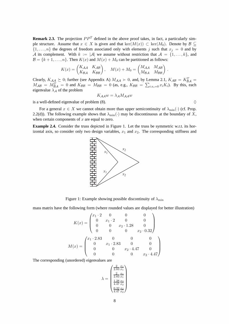
For a generalx ∈ X we cannot obtain more than upper semicontinuity ofλmin(·) (cf. Prop.2.2(d)). The following example shows thatλmin(·) may be discontinuous at the boundary ofX,when certain components ofx are equal to zero.

Example 2.4. Consider the truss depicted in Figure 1. Let the truss be symmetric w.r.t. its hor-izontal axis, so consider only two design variables,x1 andx2. The corresponding stiffness and

x1

x1

x2

x2

Figure 1: Example showing possible discontinuity ofλmin

mass matrix have the following form (where rounded values are displayed for better illustration)

K(x) =

x1 · 2 0 0 00 x1 · 2 0 00 0 x2 · 1.28 00 0 0 x2 · 0.32

M(x) =

x1 · 2.83 0 0 00 x1 · 2.83 0 00 0 x2 · 4.47 00 0 0 x2 · 4.47

The corresponding (unordered) eigenvalues are

λ =

22.83

x1

x1

22.83

x1

x1

1.284.47

x2

x2

0.324.47

x2

x2

8

The functionλmin has then the following values

λmin(x) =0.32

4.47≈ 0.07 for x2 > 0

λmin(x) =2

2.83≈ 0.71 for x2 = 0

and is thus discontinuous atx2 = 0. The reason for the discontinuity lies in the fact that, whenx2 = 0 the eigenvalue0.32

4.47x2

x2becomes undefined andλmin “jumps” to what was before the second

smallest eigenvalue. ♦

Remark 2.5. Example 4.5 will indicate thatλmin(·) may not even be Lipschitz continuous nearthe boundary ofX. ♦

2.2 The original formulations

We first give three formulations of the truss design problem that are well-known in the engineeringliterature. These formulations are obtained by just “writing down” the primal requirements andnatural constraints.

The minimum volume problem In the traditional formulation of the truss topology problem,one minimizes the weight of the truss subject to equilibriumconditions and constraints on thesmallest eigenfrequency.

minx∈Rm, u∈R

n·nℓ

m∑

i=1

xi (Pvol)

subject to(

m∑

i=1

xiKi

)uℓ = fℓ, ℓ = 1, . . . , nℓ

fTℓ uℓ ≤ γ, ℓ = 1, . . . , nℓ

xi ≥ 0, i = 1, . . . ,m

λmin(x) ≥ λ .

Hereγ is a given upper bound on the compliance of the optimal structure andλ > 0 is a giventhreshold eigenvalue. Objective function of this problem is the function(x, u) 7→

∑xi. Notice

that the eigenvalue constraint is discontinuous (see Example 2.4); this (and not only this) makesthe problem rather difficult.

The minimum compliance problem In this formulation one minimizes the worst-case compli-ance (maximizes the stiffness) of the truss subject to equilibrium conditions and constraints on the

9

minimum eigenfrequency.

minx∈Rm,u∈R

n·nℓ

max1≤ℓ≤nℓ

fTℓ uℓ (Pcompl)

subject to(

m∑

i=1

xiKi

)uℓ = fℓ, ℓ = 1, . . . , nℓ

m∑

i=1

xi ≤ V

xi ≥ 0, i = 1, . . . ,m

λmin(x) ≥ λ .

HereV > 0 is an upper bound on the volume of the optimal structure and, again, λ > 0 is agiven threshold eigenvalue. For this problem, the objective function is the nonsmooth function(x, u) 7→ max

1≤ℓ≤nℓ

fTℓ uℓ. Again, notice that the eigenvalue constraint is not continuous.

The problem of maximizing the minimal eigenvalue Here we want to maximize the smallesteigenvalue of (8) subject to equilibrium conditions and constraints on the compliance and vol-ume. Maximization of the smallest eigenfrequency is of paramount importance in many industrialapplication, e.g., in civil engineering.

maxx∈Rm,uℓ∈Rn

λmin(x) (Peig)

subject to(

m∑

i=1

xiKi

)uℓ = fℓ, ℓ = 1, . . . , nℓ

fTℓ uℓ ≤ γ, ℓ = 1, . . . , nℓ

m∑

i=1

xi ≤ V

xi ≥ 0, i = 1, . . . ,m .

Here the objective function is(x, u) 7→ λmin(x), which is a possibly discontinuous function.This discontinuity is the reason that a standard perturbation approach widely used by practitionersfor the solution of (Peig) may fail. If, with some smallǫ > 0, the nonnegativity constraints arereplaced by the constraintsxi ≥ ε for all i, and ifx∗

ε denotes a solution of this perturbed problem(together with someu∗

ε), thenx∗ε may not converge to some solutionx∗ of the unperturbed problem

(cf. Ex. 2.4 above).

We mention that each of the above three problems has already been considered in the literaturewith more or less small modifications, and that all problems find valuable interest in practicalapplications (cf. [15, 17, 11]). To the knowledge of the authors, however, a rigorous treatment ofthese problems in the situation of positive semidefinite matricesK andM (i.e., permittingxi = 0for somei, as needed in topology optimization) has not been considered, so far.

2.3 Interrelations of original formulations for M0 = 0

In this section we study relations of the three problems (Pvol), (Pcompl), and (Peig) whenM0 = 0.These relations are directly given by rescaling arguments but will also appear as special cases of

10

problems with arbitraryM0 treated in the next section. Note that in the following theorems wedo not discuss theexistenceof solutions. Instead, we discuss their interrelations when existence isguaranteed. We start with an auxiliary result.

Lemma 2.6. Let (x, u) ∈ Rm × R

n·nℓ, x ≥ 0, satisfy the equilibrium condition

K(x)uℓ = fℓ (15)

for some load vectorfℓ. ThenfTℓ uℓ > 0 and

m∑

i=1

xi > 0.

Proof. Because each of the matricesKi is symmetric and positive semidefinite, it is clear thatfT

ℓ uℓ = uTℓ K(x)uℓ ≥ 0. Assume thatfT

ℓ uℓ = 0. ThenuTℓ K(x)uℓ = 0, and simple linear algebra

shows thatK(x)uℓ = 0Rn . (16)

Eqn. (16), however, is a contradiction to the assumptions (15) and (1). Ifm∑

i=1

xi = 0 thenx = 0,

and the contradiction to (15) and (1) is obvious.

Next we observe that the functionλmin( . ) is independent of scaling of the structure, pro-vided M0 = 0. Recall thatλmin(x) is a well-defined non-negative number for anyx ∈ X (seeProp. 2.2(a)).

Lemma 2.7. LetM0 = 0 andx ≥ 0 be any vector. Then

λmin(µx) = λmin(x) for all µ > 0.

Proof. BecauseK( · ) andM( · ) are linear functions, the eigenvalue equationK(µx)v = λM(µx)v is equivalent toK(x)v = λM(x)v for all µ > 0.

We first show that each solution of (Pvol) immediately leads to a solution of (Pcompl).

Theorem 2.8. LetM0 = 0 and(x∗, u∗) be a solution of(Pvol).

(a) Then max1≤ℓ≤nℓ

fTℓ u∗

ℓ = γ.

(b) PutV :=m∑

i=1x∗

i in problem(Pcompl) and copy the value ofλ from problem(Pvol). Then

(x∗, u∗) is optimal for(Pcompl) with optimal objective function valueγ.

Proof. For the proof of (a), denote

γ∗ := max1≤ℓ≤nℓ

fTℓ u∗

ℓ .

We must show thatγ∗ = γ. Due to Lemma 2.6 we have

γ∗ > 0 and V ∗ :=∑

x∗i > 0.

Consider the couple

(x∗, u∗) :=(γ∗

γx∗,

γ

γ∗u∗)

;

11

by the definition ofγ∗ we obtain

fTℓ u∗

ℓ =γ

γ∗fT

ℓ u∗ℓ ≤

γ

γ∗γ∗ = γ for all ℓ = 1, . . . , nℓ, (17)

and, obviously,(

m∑

i=1

x∗i Ki

)u∗

ℓ =γ∗γ

γγ∗

(m∑

i=1

x∗i Ki

)u∗

ℓ = fℓ for all ℓ = 1, . . . , nℓ.

This, together with Lemma 2.7, shows that(x∗, u∗) is feasible for (Pvol). Hence optimality of(x∗, u∗) in (Pvol) yields

V ∗ ≤

m∑

i=1

x∗i =

γ∗

γ

m∑

i=1

x∗i =

γ∗

γV ∗.

BecauseV ∗ > 0, this meansγ ≤ γ∗.

Eqn. (17), however, shows thatγ∗ ≤ γ. All in all, we arrive atγ∗ = γ, as stated in (a).

Now we prove (b). Due to the choice ofV it is clear that(x∗, u∗) is feasible for problem(Pcompl). Moreover, (a) shows that the corresponding objective function value isγ. Let (x, u)be an arbitrary feasible point of (Pcompl). Lemma 2.6 shows that the valueγ := max

1≤ℓ≤nℓ

fTℓ uℓ is

positive, and hence the couple

(x, u) :=(γ

γx,

γ

γu)

is well-defined. As in (a), we conclude that(x, u) is feasible for (Pvol). Optimality of (x∗, u∗) in(Pvol) gives

m∑

i=1

x∗i ≤

m∑

i=1

xi =γ

γ

m∑

i=1

xi. (18)

Now,m∑

i=1x∗

i = V by the definition ofV , and we havem∑

i=1xi ≤ V by the feasibility of(x, u) for

(Pcompl). Hence (18) becomesV ≤ γγ V which in turn means thatγ ≤ γ. Thus we have shown

(use (a)) thatmax

1≤ℓ≤nℓ

fTℓ u∗

ℓ ≤ max1≤ℓ≤nℓ

fTℓ uℓ,

i.e., optimality of(x∗, u∗) for problem (Pcompl).

The first assertion of the theorem shows that, whenM0 = 0, the compliance constraint in(Pvol) is always active for at least one load case. Later we will demonstrate this theorem by meansof a numerical example (see Ex. 4.1).

A completely analogous theorem to Thm. 2.8 can be stated whenproblems (Pvol) and (Pcompl)are interchanged. The proof uses the same arguments and is thus omitted.

Theorem 2.9. LetM0 = 0 and let(x∗, u∗) be a solution of(Pcompl).

(a) Thenm∑

i=1x∗

i = V .

(b) Putγ := max1≤ℓ≤nℓ

fTℓ u∗

ℓ in problem(Pvol) and copyλ from (Pcompl). Then(x∗, u∗) is optimal

for (Pvol) with optimal objective function valueV .

12

The interrelations of (Pvol) (resp., of (Pcompl)) and (Peig) are a bit more cumbersome becausethe objective function (Peig) is invariant with respect to scaling, as shown in Lemma 2.7.As a firstand simple result, we obtain the following proposition (where all sums run overi = 1, . . . ,m).

Proposition 2.10. LetM0 = 0, and let(x∗, u∗) be a solution of problem(Peig).

(a) Then for each

µ ∈[∑x∗

i

V;

γ

max1≤ℓ≤nℓ

fTℓ u∗

ℓ

](19)

the couple( 1µx∗, µu∗) is also a solution of(Peig).

(b) In particular, ( V∑x∗

i

x∗,

∑x∗

i

Vu∗)

is also a solution of(Peig) where the volume constraint is attained as an equality.

(c) Analogously to (b),( max

1≤ℓ≤nℓ

fTℓ u∗

ℓ

γx∗,

γ

max1≤ℓ≤nℓ

fTℓ u∗

ℓ

u∗)

is also a solution of(Peig) where the compliance constraint is attained as an equality for atleast one load caseℓ.

Proof. First, feasibility of(x∗, u∗) in (Peig) and Lemma 2.6 yield

0 <

∑x∗

i

V≤ 1 ≤

γ

max1≤ℓ≤nℓ

fTℓ u∗

ℓ

,

and hence the interval in (19) is well-defined and non-empty.Moreover, it is straightforward tosee that ∑ 1

µx∗

i ≤ V and fTℓ u∗

ℓ ≤ γ for all ℓ = 1, . . . , nℓ

hold if and only ifµ satisfies (19). Thus for eachµ from (19), the point( 1µx∗, µu∗) is feasible in

problem (Peig). Hence Lemma 2.7 shows that it is even an optimal solution. Assertions (b) and(c) are straightforward consequences of (a).

This proposition relies on the fact that, forM0 = 0, λmin(·) is invariant with respect to scalingof the structure. Hence, if either the volume constraint or the compliance constraints are inactiveat the optimum, the optimal structure can be scaled without changing the value of the objectivefunctionλmin(·). This shows that (forM0 = 0) problem (Peig) rather looks for an optimal “shape”of the structure independently of the appropriate scaling.Later in Section 4 will see a numericalexample illustrating Prop. 2.10 (see Ex. 4.3).

2.4 Interrelations of original formulations for arbitrary M0

In this section, we do not make any restrictions onM0 apart from the general requirements alreadymentioned, i.e., thatM0 is symmetric and positive semidefinite. In the following, when relatingtwo different optimization problems, the matrixM0 is considered to be the same in both problems.

We start with a general result on the relation of optimization problems where the objectivefunction of one problem acts as a constraint of the other one and vice versa. Through this resultwe will then be able to state all interrelationships of the formulations (Pvol), (Pcompl), and (Peig).

13

Theorem 2.11.Let Y j Rk be non-empty, and let the functionsf1, f2 : Y −→ R be given. For

f1, f2 ∈ R define the two optimization problems

miny∈Y

{ f1(y) | f2(y) ≤ f2 } (P1[f2])

andminy∈Y

{ f2(y) | f1(y) ≤ f1 }. (P2[f1])

Letf2 be fixed and the setY ∗1 of solutions to problem(P1[f2]) be non-empty. The optimal function

value is denoted byf∗1 := f1(y

∗) for all y∗ ∈ Y ∗1 .

Putf∗2 := inf{ f2(y

∗) | y∗ ∈ Y ∗1 }, (20)

and let the infimum be attained at somey∗ ∈ Y ∗1 . Consider problem(P2[f1]) with f1 := f∗

1 .Theny∗ is optimal for problem(P2[f1]) with optimal objective function valuef∗

2 .

Proof. Optimality, and hence feasibility, ofy∗ for (P1[f2]) shows that this point is also feasiblefor (P2[f1]) due to the definition off1 := f∗

1 . By the choice ofy∗, the value of the objectivefunction of y∗ in (P2[f1]) is f∗

2 . Now, lety be an arbitrary feasible point of (P2[f1]) with

f2(y) ≤ f∗2 . (21)

We must prove thatf2(y) ≥ f∗2 .

First, the choice ofy∗ shows that

f∗2 = f2(y

∗) ≤ f2.

Hence, using (21), we see thatf2(y) ≤ f2.

Thus, due to feasibility ofy in (P2[f1]), it is clear that(x, u) is also feasible for (P1[f2]). Thedefinition off1 and the optimality ofy∗ for (P1[f2]) show that

f1 = f∗1 = f1(y

∗) ≤ f1(y). (22)

The feasibility of(x, u) for (P2[f1]), however, shows that

f1(y) ≤ f1

which together with (22) and with the definitionf1 := f∗1 proves

f1(y) = f∗1 .

We conclude thaty is optimal for (P1[f2]), i.e.,y ∈ Y ∗1 . Hence, by the definition off∗

2 ,

f2(y) ≥ f∗2 ,

and the proof is complete.

14

Now we collect certain tools which are needed to show that theinfimum in (20) is attained inall situations. For this, we define the function

c : {x ∈ Rm | x ≥ 0 } −→ R ∪ {+∞},

x 7→ sup1≤ℓ≤nℓ

supuℓ∈Rn

{2fT

ℓ uℓ − uTℓ

( m∑i=1

xiKi

)uℓ

}.

Obviously, the functionc denotes the maximum (over all load cases) of the negative minimumpotential energies of the structurex.

Proposition 2.12(Properties of the functionc).

(a) Letx ≥ 0. Thenc(x) < +∞ if and only if there exist “displacement vectors”u1, . . . , unℓ∈

Rn such that

K(x)uℓ = fℓ for all ℓ = 1, . . . , nℓ. (23)

(b) Letx ≥ 0. If c(x) < +∞ then

c(x) = max1≤ℓ≤nℓ

fTℓ uℓ

for all u1, . . . , unℓwhich satisfy (23).

(c) The functionc(·) is finite and continuous on the set{x ∈ Rm | x > 0} and lower semi-

continuous (l.s.c.) on{x | x ≥ 0}, i.e.,

lim infx→x

x≥0

c(x) ≥ c(x), x ≥ 0.

Proof. All assertions were proved in [1]. Assertions (a) and (b), however, are easily deduced fromthe necessary and sufficient conditions of the inner sup-problems overuℓ and from the fact thata convex quadratic function is unbounded if and only if it does not possess a stationary point.Concerning (c), we mention that the finiteness ofc on {x | x > 0} is based on assumption (5),and thatc possesses much stronger continuity properties than just being l.s.c. on{x | x ≥ 0} (see[1]).

For simplification of notation, we define

vol(x) :=m∑

i=1

xi

for x ∈ Rm, x ≥ 0. Moreover, we define

S∗vol,S

∗compl,S

∗eig ⊂ {x ∈ R

m | x ≥ 0} × Rn·nℓ

as the solution sets of the problems (Pvol), (Pcompl), and (Peig), respectively. Notice that these setsmay well be empty.

Our first result based on Thm. 2.11 relates problem (Pvol) with the problems (Pcompl) and(Peig), respectively.

Theorem 2.13. Let S∗vol be non-empty. Denote the optimal function value of problem(Pvol) by

V ∗, i.e.,

V ∗ :=

m∑

i=1

x∗i for all (x∗, u∗) ∈ S∗

vol.

15

Putγ∗ := inf

{max

1≤ℓ≤nℓ

fTℓ u∗

ℓ

∣∣∣ (x∗, u∗) ∈ S∗vol

}, (24)

andλ∗ := sup

{λmin(x

∗)∣∣∣ (x∗, u∗) ∈ S∗

vol

}. (25)

Then the following assertions hold:

(a) The infimum in (24) is attained at some(x∗, u∗) ∈ S∗vol. Moreover, withV := V ∗, and

with λ copied from problem(Pvol), the point(x∗, u∗) is optimal for problem(Pcompl) withoptimal objective function valueγ∗.

(b) The supremum in (25) is attained at some(x∗, u∗) ∈ S∗vol. Moreover, withV := V ∗, and

with γ copied from problem(Pvol), the point(x∗, u∗) is optimal for problem(Peig) withoptimal objective function valueλ∗.

Proof. Consider the setX ∗

vol := {x∗ | (x∗, u∗) ∈ S∗vol}.

Using Prop. 2.12(a) and (b) it is easy to see that

X ∗vol =

{x ≥ 0

∣∣∣ vol(x) = V ∗, c(x) ≤ γ, λmin(x) ≥ λ}

. (26)

Becausex ≥ 0 andvol(x) = V ∗ for all x ∈ X ∗vol, the setX ∗

vol is bounded. Moreover, becausevol(·) is continuous,λmin(·) is u.s.c. (see Prop. 2.2(d)), andc(·) is l.s.c. (see Prop. 2.12(c)), the setX ∗

vol is closed. All in all,X ∗vol is a compact set.

We first prove (a). Proposition 2.12(a) and (b) shows that

γ∗ = inf{ c(x) | x ∈ X ∗vol }, (27)

and that the infimum in (24) is attained if and only if the infimum in (27) is attained. The latter,however, is straightforward becausec(·) is a l.s.c. function, andX ∗

vol is a compact set (each l.s.c.function attains its infimum on a compact set; see, e.g., [13,Thm. 2.13.1]). The rest of the assertionfollows directly from Thm. 2.11 with the settings

Y := { (x, u) ∈ Rm × R

n·nℓ | K(x)uℓ = fℓ, ℓ = 1, . . . , nℓ,xi ≥ 0, i = 1, . . . ,m,

λmin(x) ≥ λ },

f1(x, u) := vol(x),

f2(x, u) := c(x),

f2 := γ,

f1 := V ∗.

The proof of (b) is analogous. We have to show that the supremum

λ∗ = sup{λmin(x) | x ∈ X ∗vol }

is attained at somex∗. This is the case becauseλmin(·) is u.s.c. (see Prop. 2.2(d)) andX ∗vol is

compact (see above). Notice thatc(x∗) ≤ γ < +∞ (see (26)), and hence corresponding vectors

16

u∗1, . . . , u

∗eℓ

exist by Prop. 2.12(a) and (b) such that(x∗, u∗) is feasible (and optimal) for (Pvol)).The rest of assertion (b) follows directly from Thm. 2.11 with the settings

Y := { (x, u) ∈ Rm × R

n·nℓ | K(x)uℓ = fℓ, ℓ = 1, . . . , nℓ,xi ≥ 0, i = 1, . . . ,m,fT

ℓ uℓ ≤ γ ℓ = 1, . . . , nℓ },

f1(x, u) := vol(x),

f2(x, u) := −λmin(x),

f2 := −λ,

f1 := V ∗.

Theorem 2.13(a) reflects the fact that at some solution(x∗, u∗) of (Pvol) none of the com-pliance constraints may be satisfied with equality, and hence the “post-optimization” in (24) isneeded to select a proper solution of (Pvol) to obtain a solution of (Pcompl). Theorem 2.13(a) alsoshows that—with the appropriate settings ofV andλ—there is always a structurex∗ which isoptimal for both problems at the same time (provided there exists a solution at all). Analogouscomments, of course, can be made for Thm. 2.13(b) concerningsolutions of (Peig). A numericalexample illustrating Thm. 2.13 is given in Section 4 (Ex. 4.4).

Theorem 2.13 substantially simplifies in the following special situation.

Corollary 2.14. Let the setX ∗vol = {x∗ | (x∗, u∗) ∈ S∗

vol} be a singleton. Then the followingassertions hold:

(a) Put V := vol(x∗) in problem(Pcompl) and copy the valueλ from problem(Pvol). Then(x∗, u∗) is optimal for problem(Pcompl) with optimal objective function valuemax

1≤ℓ≤nℓ

fTℓ u∗

ℓ .

(b) PutV := vol(x∗) in problem(Peig) and copy the valueγ from problem(Pvol). Then(x∗, u∗)is optimal for problem(Peig) with optimal objective function valueλmin(x

∗).

Proof. If X ∗vol = {x∗} then the infimum in (24) is attained at any(x∗, u∗) ∈ S∗

vol because for eachu∗, u∗ with K(x∗)u∗

ℓ = K(x∗)u∗ℓ = fℓ for all ℓ the compliance values

fTℓ u∗

ℓ = u∗Tℓ K(x∗)u∗

ℓ = u∗Tℓ fℓ = fT

ℓ u∗ℓ , ℓ = 1, . . . , nℓ

are constant. BecauseX ∗vol is the singletonx∗, and becauseλmin(·) does not depend onu∗, it is

trivial to see that the supremum in (25) is attained at each(x∗, u∗) ∈ S∗vol. Now apply Thm. 2.13.

Remark 2.15. Theorem 2.13(a) generalizes Thm. 2.8(b) of the previous chapter. If M0 = 0 inThm. 2.13(a) then Thm. 2.8(a) shows that

max1≤ℓ≤nℓ

fTℓ u∗

ℓ = γ for all (x∗, u∗) ∈ S∗vol.

Henceγ∗ = γ, and the infimum in (24) is attained at each solution(x∗, u∗) ∈ S∗vol. Similar

comment cannot be made for Thm. 2.13(b). The settingM0 = 0 does not guarantee that foreach solution(x∗, u∗) of (Pvol) the eigenvalue constraint is attained as an equality. Thiswill alsobe demonstrated by Example 4.4 below. The background lies inthe invariance ofλmin(·) w.r.t.scaling of the structure; see Lemma 2.7. ♦

17

Analogously to Thm. 2.13, we may derive solutions of problems (Pvol) and (Peig), respec-tively, from solutions of problem (Pcompl).

Theorem 2.16.LetS∗compl be non-empty. Denote the optimal function value of problem(Pcompl)

byγ∗, i.e.,γ∗ := max

1≤ℓ≤nℓ

fTℓ u∗

ℓ for all (x∗, u∗) ∈ S∗compl.

Put

V ∗ := inf{ m∑

i=1

x∗i

∣∣∣ (x∗, u∗) ∈ S∗compl

}, (28)

andλ∗ := sup

{λmin(x

∗)∣∣∣ (x∗, u∗) ∈ S∗

compl

}. (29)

Then the following assertions hold:

(a) The infimum in (28) is attained at some(x∗, u∗) ∈ S∗compl. Moreover, withγ := γ∗, and

with λ copied from problem(Pcompl), the point(x∗, u∗) is optimal for problem(Pvol) withoptimal objective function valueV ∗.

(b) The supremum in (29) is attained at some(x∗, u∗) ∈ S∗compl. Moreover, withγ := γ∗, and

with V copied from problem(Pcompl), the point(x∗, u∗) is optimal for problem(Peig) withoptimal objective function valueλ∗.

Proof. We modify the proof of Thm. 2.13. Consider the set

X ∗compl := {x∗ | (x∗, u∗) ∈ S∗

compl}.

In view of Prop. 2.12(a) and (b) it is easy to see that

X ∗compl =

{x ≥ 0

∣∣∣ vol(x) ≤ V , c(x) = γ∗, λmin(x) ≥ λ}

. (30)

Becauseγ∗ is the optimal objective function value, there is nox ≥ 0 such thatvol(x) ≤ V ,c(x) < γ∗, andλmin(x) ≥ λ. Hence the setX ∗

compl remains unchanged if we change the equalitysign in “c(x) = γ∗” to an inequality sign:

X ∗compl =

{x ≥ 0

∣∣∣ vol(x) ≤ V , c(x) ≤ γ∗, λmin(x) ≥ λ}

. (31)

Becausex ≥ 0 andvol(x) ≤ V for all x ∈ X ∗compl, the setX ∗

compl is bounded. Moreover, eachof the functionsvol(·), −λmin(·), andc(·) is l.s.c. (see Props. 2.2(d) and 2.12(c)). Hence thedescription (31) shows thatX ∗

compl is a closed set, and thusX ∗compl is compact (notice that thelevel

line of a l.s.c. functionf(·) for some valueα, i.e., the set{y | f(y) = α}, needs not be closed, butthe level set{y | f(y) ≤ α} is always closed).

First we prove (a). Obviously, the infimum in (28) is attainedbecauseX ∗compl is a compact set

andvol(·) is continuous. Now apply Thm. 2.11 with the settings

Y := { (x, u) ∈ Rm × R

n·nℓ | K(x)uℓ = fℓ, ℓ = 1, . . . , nℓ,xi ≥ 0, i = 1, . . . ,m,

λmin(x) ≥ λ },

f1(x, u) := max1≤ℓ≤nℓ

fTℓ uℓ,

f2(x, u) := vol(x),

f2 := V ,

f1 := γ∗.

18

The proof of (b) is analogous to that of Thm. 2.13(b).

The following corollary parallels Cor. 2.14. Its proof is even simpler because neithervol(·)norλmin(·) in (28) and (29), respectively, depend onu∗.

Corollary 2.17. Let the setX ∗compl = {x∗ | (x∗, u∗) ∈ S∗

compl} be a singleton. Then the followingassertions hold:

(a) Putγ := max1≤ℓ≤nℓ

fTℓ u∗

ℓ in problem(Pvol) and copy the valueλ from problem(Pcompl). Then

(x∗, u∗) is optimal for problem(Pvol) with optimal objective function valuevol(x∗).

(b) Putγ := max1≤ℓ≤nℓ

fTℓ u∗

ℓ in problem(Peig) and copy the valueV from problem(Pcompl). Then

(x∗, u∗) is optimal for problem(Peig) with optimal objective function valueλmin(x∗).

Remark 2.18. Similarly as in Remark 2.15, Thm. 2.16(a) generalizes Thm. 2.9(b) of the previoussection. IfM0 = 0 in Thm. 2.16(a) then Thm. 2.9(a) shows that

vol(x∗) = V for all (x∗, u∗) ∈ S∗compl.

HenceV ∗ = V , and the infimum in (28) is attained at each solution(x∗, u∗) ∈ S∗compl. ♦

Finally, we may derive solutions of problems (Pvol) and (Pcompl) from solutions of (Peig).

Theorem 2.19.LetS∗eig be non-empty. Denote the optimal function value of problem(Peig) byλ∗,

i.e.,λ∗ := λmin(x

∗) for all (x∗, u∗) ∈ S∗eig.

Put

V ∗ := inf{ m∑

i=1

x∗i

∣∣∣ (x∗, u∗) ∈ S∗eig

}, (32)

andγ∗ := inf

{max

1≤ℓ≤nℓ

fTℓ u∗

ℓ

∣∣∣ (x∗, u∗) ∈ S∗eig

}. (33)

Then the following assertions hold:

(a) The infimum in (32) is attained at some(x∗, u∗) ∈ S∗eig. Moreover, withλ := λ∗, and with

γ copied from problem(Peig), the point(x∗, u∗) is optimal for problem(Pvol) with optimalobjective function valueV ∗.

(b) The infimum in (33) is attained at some(x∗, u∗) ∈ S∗eig. Moreover, withλ := λ∗, and

with V copied from problem(Peig), the point(x∗, u∗) is optimal for problem(Pcompl) withoptimal objective function valueγ∗.

Proof. The proof of this Theorem is analogous to that of Thm. 2.13 with the role of the functionsvol(·) andλmin(·) interchanged.

For illustration of this theorem, we refer to Example 4.3. The proof of the following corollaryis analogous to that of Cor. 2.14.

Corollary 2.20. Let the setX ∗eig = {x∗ | (x∗, u∗) ∈ S∗

eig} be a singleton. Then the followingassertions hold:

(a) Put λ := λmin(x∗) in problem (Pvol) and copy the valueγ from problem(Peig). Then

(x∗, u∗) is optimal for problem(Pvol) with optimal objective function valuevol(x∗).

19

(b) Putλ := λmin(x∗) in problem(Pcompl) and copy the valueV from problem(Peig). Then

(x∗, u∗) is optimal for problem(Pcompl) with optimal objective function valuemax1≤ℓ≤nℓ

fTℓ u∗

ℓ .

To conclude this theoretical study of relations of the threeoriginal problem formulations wewould like to give a few comments on their practical use. Obviously, a direct implementation ofone of the Theorems 2.13, 2.16, and 2.19 for numerical purposes is difficult because one wouldneed to know the set ofall solutions to one of the problems, or one should be able to solve theinf- or sup-problems on the optimal set. There are ways to do this, as has been recently shownin [8]. However, as we will see in Section 3, there is no need toproceed from a solution of one(nonlinear!) problem to the solution of some other problem,because global solutions of some ofthe original problems can be calculated through equivalent(quasi)convex problem formulations.

2.5 Brief discussion on the variation ofM0

In this section we want to briefly prove what is widely known among practicioners: what happenswhen the non-structural mass is changed or even removed. Forexample, if volume minimizationis considered then a bigger non-structural mass will generally increase the optimal volume. Sim-ilarly, if maximization of the minimal eigenvalue is considered, the removal of the non-structuralmass will generally lead to a smaller minimal eigenvalue. Hence, in this section, we briefly con-sider the variation ofM0 and use the extended notation (see Prop. 2.2(c))

λmin(x,M0) := sup{λ | K(x) − λ(M(x) + M0) � 0}. (34)

Lemma 2.21. Let x ≥ 0, and letM0,M0 ∈ Rn×n be symmetric withM0 � M0 � 0. Then

λmin(x, M0) ≤ λmin(x,M0).

Proof. Putλ := λmin(x, M0). Then

0 � K(x) − λ(M(x) + M0) = K(x) − λM(x) − λM0

� K(x) − λM(x) − λM0 = K(x) − λ(M(x) + M0).

Hence,λ ≤ sup{λ | K(x) − λ(M(x) + M0) � 0} = λmin(x,M0).

As a simple conclusion concerning the optimal objective function values of our three problemswe obtain

Proposition 2.22. Consider two problems of the type(Pvol) (or (Pcompl) or (Peig)), with the sameconstraint boundsγ andλ (resp.V andλ, resp.V andγ) but with different non-structural massmatricesM0, M0 whereM0 � M0. Let both problems possess a solution, and denote the optimalobjective function values byV ∗, V ∗ (resp.γ∗, γ∗, resp.λ∗, λ∗). ThenV ∗ ≥ V ∗ (resp.γ∗ ≥ γ∗,resp.λ∗ ≤ λ∗).

Proof. Consider the pair of minimum volume problems. Notice that each feasible point(x, u) ofproblem (Pvol) with non-structural massM0 is also feasible for the problem with non-structuralmassM0 due to Lemma 2.21(a). Hence,V ∗ ≤ V ∗.

The proof for the pair of min-max compliance problems is analogous. For the pair of max-min eigenvalue problems it is even simpler, because the set of feasible points is the same for bothproblems, and Lemma 2.21(a) applies directly on the objective function values. (Notice that forthis type of problems, we aremaximizing, and thus we have “≤” in the assertion.)

20

More detailed results than in the above proposition can hardly be obtained, apart from theeffect of simple joint scalings of the boundsV , γ, λ andM0. Because the total mass matrix in theproblem is(M(x) + M0), a pure change of onlyM0 always has nonlinear impact in the problem,and hence, is difficult to describe. As a consequence, the optimal topology changes as well with achange ofM0. Such a numerical example is presented Section 4 (see Ex. 4.6).

3 SDP reformulations

All the original formulations are nonconvex, some even discontinuous. Furthermore, all of themimplicitly include the computation of the smallest eigenvalue of (8). Below we give reformulationsof the problems (Pvol), (Pcompl), (Peig) to problems that are much easier to analyze and to solvenumerically. All these reformulations have been known. Thethird one, however, has never beenused for the numerical treatment, up to our knowledge. We will further use a unified approach tothese reformulation that offers a clear look at their mutualrelations.

We start with an auxiliary result.

Proposition 3.1. Letx ∈ Rm, x ≥ 0, andγ ∈ R be fixed, and fix an indexℓ ∈ {1, . . . , nℓ}. Then

there existsuℓ ∈ Rn satisfying

K(x)uℓ = fℓ and fTℓ uℓ ≤ γ

if and only if (γ −fT

ℓ

−fℓ K(x)

)� 0 .

Proof. Note thatK(x) may be singular in our case, so that we cannot directly use theSchurcomplement theorem. We first write the matrix inequality equivalently as

α2γ − 2αfTℓ v + vT K(x)v ≥ 0 ∀α ∈ R,∀v ∈ R

n . (35)

“⇒” As K(x) � 0, we know thatuℓ minimizes the quadratic functionalv 7→ vT K(x)v−2fTℓ v

with the minimal value−fTℓ uℓ. Thus

vT K(x)v − 2fTℓ v ≥ −fT

ℓ uℓ ≥ −γ ∀v ∈ Rn .

Using the substitutionv = σw, σ ∈ R, we can write this as

(σw)T K(x)(σw) − 2fTℓ (σw) ≥ −γ ∀σ ∈ R,∀w ∈ R

n ,

hence

wT K(x)w −1

σ2fT

ℓ w ≥ −1

σ2γ ∀σ ∈ R \ {0},∀w ∈ R

n

which is just (35) withα = 1σ .

“⇐” Put α = 12 ; then we get from (35)

1

4γ + vT (K(x)v − fℓ) ≥ 0 ∀v ∈ R

n

and soK(x)v = fℓ .

Inserting this into (35) withα = 1, we haveγ + vT (fℓ − 2fℓ) ≥ 0, that is,γ ≥ fTℓ v, and we are

done.

With this proposition, we immediately get the following reformulations of our three originalproblems.

21

The minimum volume problem In this problem,γ andλ are given, and we minimize the upperboundV on the volume.

minx∈Rm,V ∈R

V (PSDPvol )

subject to(

γ −fTℓ

−fℓ K(x)

)� 0, ℓ = 1, . . . , nℓ

m∑

i=1

xi ≤ V

xi ≥ 0, i = 1, . . . ,m

K(x) − λ(M(x) + M0) � 0 .

We mention that this problem has first been formulated and studied in [14].

The minimum compliance problem HereV andλ are given, and we minimize the upper boundγ on the compliance.

minx∈Rm,γ∈R

γ (PSDPcompl)

subject to(

γ −fTℓ

−fℓ K(x)

)� 0, ℓ = 1, . . . , nℓ

m∑

i=1

xi ≤ V

xi ≥ 0, i = 1, . . . ,m

K(x) − λ(M(x) + M0) � 0 .

The problem of maximizing the minimal eigenvalue Now γ andV are given, andλ is thevariable. For the sake of a common problem structure in all three formulations, weminimizeandput a minus in front of the objective function.

minx∈Rm,λ∈R

−λ (PSDPeig )

subject to(

γ −fTℓ

−fℓ K(x)

)� 0, ℓ = 1, . . . , nℓ

m∑

i=1

xi ≤ V

xi ≥ 0, i = 1, . . . ,m

K(x) − λ(M(x) + M0) � 0 .

The proof of the following proposition is immediate, and thus is skipped.

Proposition 3.2. (a) If (x∗, u∗) is a global minimizer of(Pvol) then(x∗, V ∗) is a global mini-mizer of (PSDP

vol ) whereV ∗ :=∑

x∗i , and the optimal values of both problems coincide.

22

(b) If (x∗, V ∗) is a global minimizer of(PSDPvol ) then there existsu∗ such that(x∗, u∗) is a global

minimizer of(Pvol), and the optimal values of both problems coincide.Analogous statements hold for the pairs of problems(Pcompl)-(PSDP

compl) and (Peig)-(PSDPeig ),

respectively, where in the latter case, the optimal function values coincide up to a sign.

Note that problems (PSDPvol ) and (PSDP

compl) are linear SDPs, while (PSDPeig ) is an SDP problem

with a bilinear matrix inequality (BMI) constraint, i.e., it is generally nonconvex. We shouldemphasize that, due to the SDP reformulation, the originally discontinuous problems became con-tinuous; a fact of big practical value.

Theorem 3.3. Each local minimizer of problem(PSDPvol ) is also a global minimizer. Analogous

statement holds for problem(PSDPcompl).

Proof. Problems (PSDPvol ) and (PSDP

compl) are linear SDPs, i.e., convex problems, and the assertionsfollow.

Needless to say that this theorem is of paramount interest from the practical point of view.Clearly, a statement similar to Thm. 3.3 does not hold for theproblem (PSDP

eig ); see Example 2.4where the functionλmin(·) is constant forx2 > 0 and has thus infinitely many local minima whichare, however, greater than the global minimum attained atx2 = 0.

We remark, however, that problem (PSDPeig ) hides aquasiconvex structure. To see this, use

Def. 2.1 to write problem (PSDPeig ) in the form

min{−λmin(x) | x ∈ F } (36)

with the feasible set

F :={

x ∈ Rm∣∣∣x ≥ 0;

(γ −fT

ℓ

−fℓ K(x)

)� 0, ℓ = 1, . . . , nℓ;

m∑

i=1

xi ≤ V}

.

Then Prop. 2.2(f) and the fact that the cone of positive semidefinite matrices is convex show thatwe minimize here a quasiconvex function over a convex feasible setF . This fact might be useful,e.g., for the application of cutting plane algorithms from global optimization. Unfortunately, thefunction−λmin(·) lacks to be strictly quasiconvex as already explained in Example 2.4.

Formulation (36) of problem (PSDPeig ) immediately clarifies the existence of solutions:

Theorem 3.4. Problem(PSDPeig ) (or, equivalently, problem(Peig)) possesses a solution if and only

if it possesses feasible points.

Proof. Consider problem (PSDPeig ) in the form (36). Since the cone of positive semidefinite matrices

is closed, the setF is compact. Moreover,0 /∈ F due to assumption (1), and hence(−λmin) isl.s.c. onF by Prop. 2.2(d). Each l.s.c. function attains its infimum on anon-empty compact set(see, e.g., [13, Thm. 2.13.1]).

Instead of using methods from global optimization for the calculation of a global minimizer ofproblem (PSDP

eig ), we may use the close relation to the convex problems (PSDPvol ) and (PSDP

compl). In

the following we propose a practical framework for finding the global solution of (PSDPeig ) based on

the solutions of a sequence of problems which are of the type (PSDPvol ). Analogous considerations

can be done with problems of the type (PSDPcompl).

23

For fixedλ ≥ 0 and fixedδ ≥ 0 consider the following linear SDP:

minx∈Rm,V ∈R

V (PSDPvol

(λ, δ))

subject to(

γ −fTℓ

−fℓ K(x)

)� 0, ℓ = 1, . . . , nℓ

m∑

i=1

xi ≤ V

V ≤ V

xi ≥ 0, i = 1, . . . ,m

K(x) − (λ + δ)(M(x) + M0) � 0 .

Notice that this problem is just problem (PSDPvol ) with the choiceλ := λ + δ, and with the sup-

plementary linear constraintV ≤ V . In the following, the feasible set of this problem is denotedby

F(λ, δ),

for simplicity. Notice that (PSDPvol

(λ, δ)) is a linear SDP, i.e., a convex optimization problem for

which a global minimizer can be calculated, providedF(λ, δ) 6= ∅. Moreover, since (PSDPvol

(λ, δ))is a convex SDP, modern solution procedures are able to recognize whetherF(λ, δ) = ∅.

The following proposition gives a tool for the estimation ofthe (globally) optimal objectivefunction value of problem (PSDP

eig ).

Proposition 3.5. Let (x, λ) be feasible for(PSDPeig ), and let (−λ∗∗) denote the (globally) opti-

mal function value of problem(PSDPeig ). Moreover, letδ > 0 be arbitrary, and consider problem

(PSDPvol

(λ, δ)) with the parametersγ and V copied from(PSDPeig ). Then the following assertions

hold:

(a) If F(λ, δ) 6= ∅ then for each(x, V ) ∈ F(λ, δ) the point(x, λ + δ) is feasible for(PSDPeig ),

i.e.,−λ∗∗ ≤ −(λ + δ) < −λ. (37)

(b) If F(λ, δ) = ∅ then−(λ + δ) < −λ∗∗ ≤ −λ. (38)

Proof. For the proof of (a), let(x, V ) ∈ F(λ, δ) be arbitrary. It is straightforward to see that(x, λ + δ) is feasible for (PSDP

eig ), and hence its objective function value(−(λ + δ)) satisfies (37).To prove (b), first notice that the second inequality in (38) is a simple consequence of(x, λ)

being feasible for (PSDPeig ). The first inequality in (38) is now proved by contradiction. Assume

that−(λ + δ) ≥ −λ∗∗, i.e., there existsx ∈ Rn such that(x, λ + δ) is feasible for (PSDP

eig ). PutV := vol(x), and consider problem (PSDP

vol(λ, δ)). Because(x, λ + δ) is feasible for (PSDP

eig ), we

see that the point(x, V ) satisfies the LMIs, the two volume constraintsV =∑

xi ≤ V , and thenon-negativity constraints in (PSDP

vol(λ, δ)). Moreover, feasibility of(x, λ + δ) for (PSDP

eig ) alsoyields thatK(x) − (λ + δ)(M(x) + M0) � 0. All in all, we obtain that(x, V ) ∈ F(λ, δ) whichcontradicts the assumption.

As an immediate consequence of Prop. 3.5 we get the followingassertion.

24

Corollary 3.6. Let (x, λ) be feasible for(PSDPeig ). Then(x, λ) is a global minimizer of(PSDP

eig ) ifand only ifF(λ, δ) = ∅ for all δ > 0.

The practical value of Prop. 3.5 lies in the possibility to improve upper and lower bounds forλ∗∗ which can be numerically calculated through solutions (or only feasible points) of convexlinear SDPs. As a pre-processing step, we first calculate initial lower and upper boundsλL

0 , λU0 on

λ∗∗. For this, first calculate a feasible point(x, λ) of (PSDPeig ) and choose arbitraryδ > 0. Then

find the smallestk ∈ N such thatF(λ, 2k δ) = ∅ by solving (PSDPvol

(λ, 2k δ)) repeatedly. Set

λL0 := λ + 2k−1δ and λU

0 := λ + 2k δ .

Then Prop. 3.5 shows that0 ≤ λL

0 ≤ λ∗∗ < λU0 . (39)

With these bounds it is easy to construct a bisection type algorithm which in each step reduces thegap(λU

k − λLk ) by a factor of (at least)12 .

Algorithm 3.1. Choose an accuracyη > 0, a feasible point(x, λ) for (PSDPeig ). Put(x0, λ0) :=

(x, λ), δ0 := 12 (λU

0 − λL0 ), andk := 0. Go to Step 2.

1. Calculate a feasible point [or even a local minimizer](xk, λk) of (PSDPeig ) with the additional

constraint “λ ≥ λLk ”.

2. If λk > λLk then updateλL

k by λLk := λk.

3. If λUk − λL

k ≤ η then EXIT with the result(x∗, λ∗) := (xk, λk).

4. Putδk := 12 (λU

k − λLk ), and consider problem (PSDP

vol(λk, δk)).

If F(λk, δk) 6= ∅ then:

4A. PutλLk+1 := λL

k + δk, k := k + 1, and go to Step 1.

Otherwise, ifF(λk, 2k δ) = ∅, then:

4B PutλUk+1 := λU

k − δl, k := k + 1, and go to Step 1.

Proposition 3.7. Let (PSDPeig ) possess a solution(x∗∗, λ∗∗) (cf. Thm. 3.4). Then the following

assertions hold.

(a) Algorithm 3.1 is well-defined, and after each iteration we have

λLk ≤ λ∗∗ < λU

k and λUk − λL

k ≤ 2−k(λU0 − λL

0 ).

(b) Algorithm 3.1 terminates after a finite numberK of iterations, and

K ≤

⌈ln(λU

0 − λL0 ) − ln(η)

ln(2)

⌉.

At termination, the result(x∗, λ∗) is feasible for(PSDPeig ) with

λ∗∗ − λ∗ ≤ η .

25

The proof of this proposition is a straightforward exercise.Notice that the additional constraint “λ ≥ λL

k ” in Step 1 does not cause any trouble but guar-antees that(λk)k is monotonically increasing. Moreover, the calculation ofglobal minimizers (inStep 4A), resp. local minimizers (in Step 1), instead of justfeasible points should significantlyspeed up the algorithm. In this case the update ofλU

k in Step 4B, resp. ofλLk in Step 2, may lead

to a much bigger reduction of the gapλUk − λU

k . Obviously, Step 1 must be carried out in eachiteration. Notice also, thatλL

k is increased in Step 4A, while it remains untouched in Steps 4B.Denote byK ′ the number of iterations in which Steps 4A have been performed. Moreover, ifSteps 4A has been performed in iterationk − 1, let (xk, λk) in Step 1 be a local optimizer. Then,consequently,

K ′ ≤∣∣∣{

λ | (x, λ) is a local optimizer of (PSDPeig )

}∣∣∣,

i.e. K ′ is limited by the number of levels of the objective function which are attained at a localoptimizer. We believe that this cardinality is very small inapplications. As an illustration considerEx. 2.4 whereK ′ = 2.

For the numerical treatment of the SDP problems (PSDPvol ), (PSDP

compl), (PSDPeig ) one must resort

to methods of semidefinite programming. Such methods, and corresponding codes, are nowadaysavailable for linear SDPs. The limiting factor of these codes is, however, the problem size which,compared to general nonlinear programs, is restricted to problems of medium size. The problem(PSDP

eig ) even requires a method which can deal with bilinear matrix inequalities. We will use sucha method to solve examples in the next section. It should be noted, however, that algorithms andcodes for SDPs with bilinear matrix inequalities are on the edge of current research and are notyet standard.

4 Numerical Examples

In this chapter we present numerical examples which, on the one hand, will illustrate some of thetheoretical results above and, on the other hand, demonstrate the practical use of the SDP problemformulations.

The code we have used for the treatment of the SDP formulations is PENBMI, version 2.0 [10].This code implements the generalized Augmented Lagrangianmethod, as described in [9, 19]. Inparticular, PENBMI can treat bilinear matrix inequalities as is necessary for problem (PSDP

eig ) [7].The examples were solved on a Pentium III-M 1GHz PC running Windows 2000. All problems

were formulated and solved in MATLAB using the YALMIP parser [12] to PENBMI.

Example 4.1. This example illustrates Thms. 2.8, 2.9, and 2.19 withM0 = 0. Consider a 3-by-3 truss with all nodes connected by potential bars. The nodeson the left-hand side are fixed inboth directions, a horizontal force(−1, 0) is applied at the right-middle node; see Figure 2-left.No nonstructural mass is considered, i.e.,M0 = 0. We consider the minimum volume problem(PSDP

vol ) with γ = 1 andλ = 5.0 · 10−2. PENBMI calculated the (global) optimal solution(x∗, V ∗)of this convex problem: the optimal designx∗ is shown in Figure 2-right, whileV ∗ = 1.20229.Prop. 3.2(b) shows that there existsu∗ such that(x∗, u∗) is optimal for problem (Pvol).

Now consider the minimum compliance problem (PSDPcompl) with V = 1.20229 andλ = 5.0 ·

10−2. As expected by Prop. 3.2(b) and Thm. 2.9, we obtain the solution (x∗, γ∗) with the samestructurex∗ as before (Fig. 2-right), and withγ∗ = 1.

Finally, when solving the problem of maximizing the minimumeigenvalue (PSDPeig ) with V =

1.20229 andγ = 1, we again obtainx∗ from before, andλ∗ = 5.0 · 10−2. This shows that thevalueV ∗ in (32) and the valueγ∗ in (33) are attained forx∗ because otherwise this would yield a

26

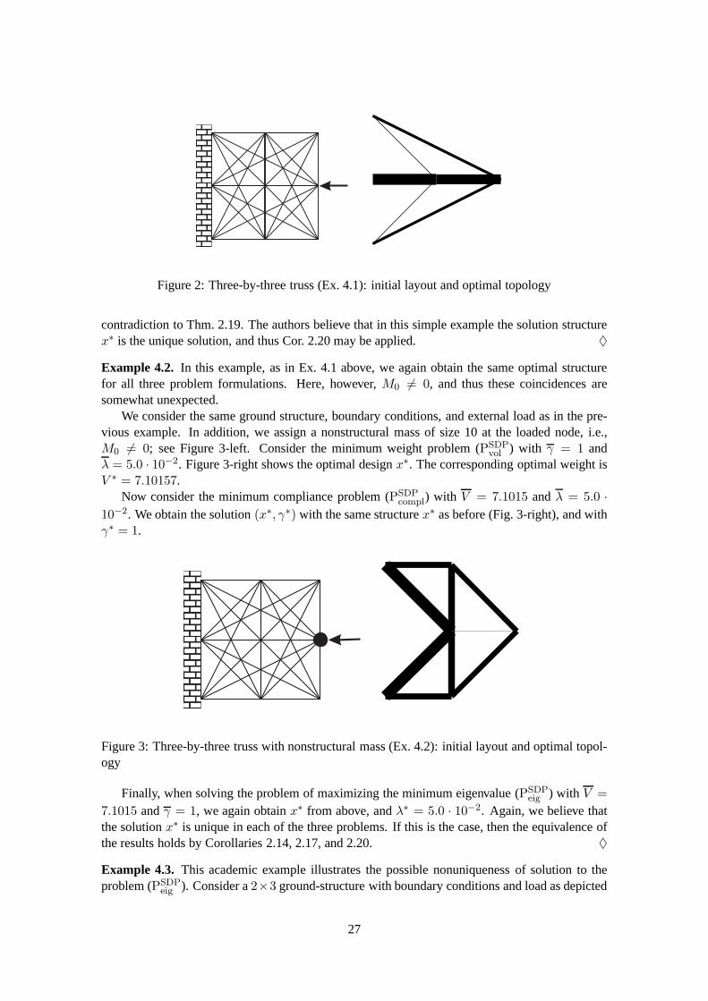
Figure 2: Three-by-three truss (Ex. 4.1): initial layout and optimal topology

contradiction to Thm. 2.19. The authors believe that in thissimple example the solution structurex∗ is the unique solution, and thus Cor. 2.20 may be applied. ♦

Example 4.2. In this example, as in Ex. 4.1 above, we again obtain the same optimal structurefor all three problem formulations. Here, however,M0 6= 0, and thus these coincidences aresomewhat unexpected.

We consider the same ground structure, boundary conditions, and external load as in the pre-vious example. In addition, we assign a nonstructural mass of size 10 at the loaded node, i.e.,M0 6= 0; see Figure 3-left. Consider the minimum weight problem (PSDP

vol ) with γ = 1 andλ = 5.0 · 10−2. Figure 3-right shows the optimal designx∗. The corresponding optimal weight isV ∗ = 7.10157.

Now consider the minimum compliance problem (PSDPcompl) with V = 7.1015 andλ = 5.0 ·

10−2. We obtain the solution(x∗, γ∗) with the same structurex∗ as before (Fig. 3-right), and withγ∗ = 1.

Figure 3: Three-by-three truss with nonstructural mass (Ex. 4.2): initial layout and optimal topol-ogy

Finally, when solving the problem of maximizing the minimumeigenvalue (PSDPeig ) with V =

7.1015 andγ = 1, we again obtainx∗ from above, andλ∗ = 5.0 · 10−2. Again, we believe thatthe solutionx∗ is unique in each of the three problems. If this is the case, then the equivalence ofthe results holds by Corollaries 2.14, 2.17, and 2.20. ♦

Example 4.3. This academic example illustrates the possible nonuniqueness of solution to theproblem (PSDP

eig ). Consider a2×3 ground-structure with boundary conditions and load as depicted

27

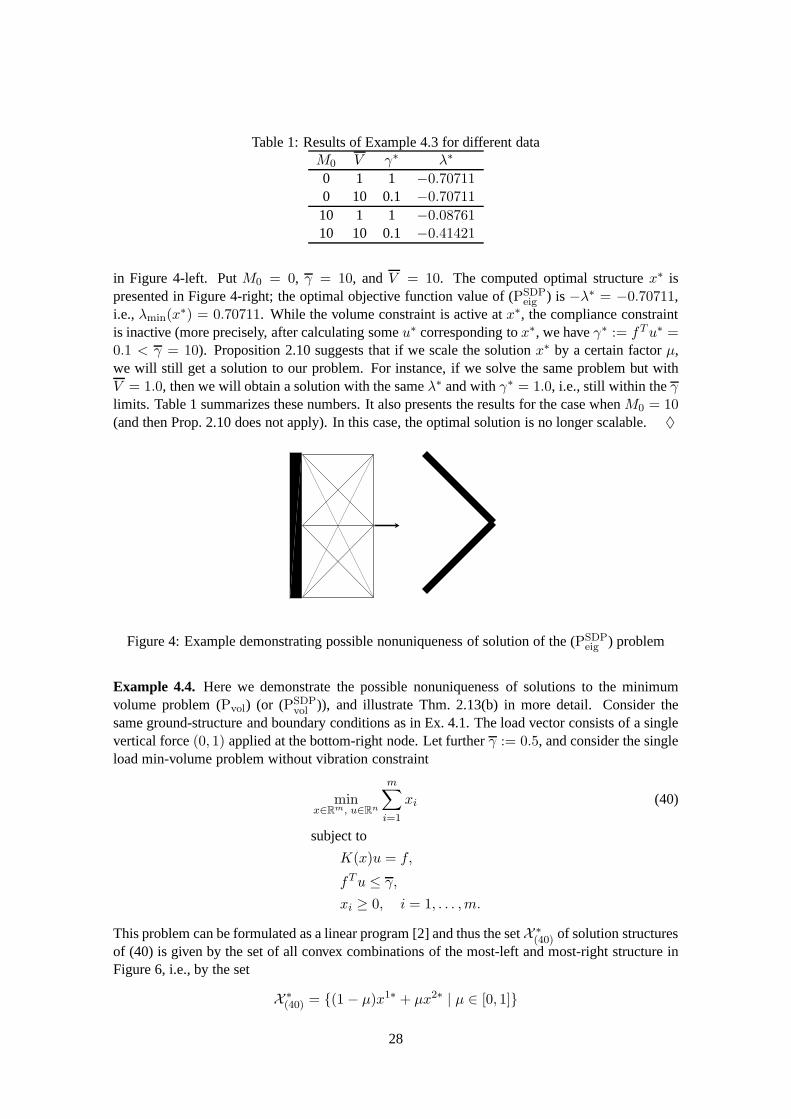
Table 1: Results of Example 4.3 for different dataM0 V γ∗ λ∗

0 1 1 −0.707110 10 0.1 −0.70711

10 1 1 −0.0876110 10 0.1 −0.41421

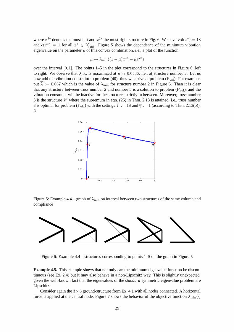
in Figure 4-left. PutM0 = 0, γ = 10, andV = 10. The computed optimal structurex∗ ispresented in Figure 4-right; the optimal objective function value of (PSDP

eig ) is −λ∗ = −0.70711,i.e.,λmin(x

∗) = 0.70711. While the volume constraint is active atx∗, the compliance constraintis inactive (more precisely, after calculating someu∗ corresponding tox∗, we haveγ∗ := fT u∗ =0.1 < γ = 10). Proposition 2.10 suggests that if we scale the solutionx∗ by a certain factorµ,we will still get a solution to our problem. For instance, if we solve the same problem but withV = 1.0, then we will obtain a solution with the sameλ∗ and withγ∗ = 1.0, i.e., still within theγlimits. Table 1 summarizes these numbers. It also presents the results for the case whenM0 = 10(and then Prop. 2.10 does not apply). In this case, the optimal solution is no longer scalable. ♦

Figure 4: Example demonstrating possible nonuniqueness ofsolution of the (PSDPeig ) problem

Example 4.4. Here we demonstrate the possible nonuniqueness of solutions to the minimumvolume problem (Pvol) (or (PSDP

vol )), and illustrate Thm. 2.13(b) in more detail. Consider thesame ground-structure and boundary conditions as in Ex. 4.1. The load vector consists of a singlevertical force(0, 1) applied at the bottom-right node. Let furtherγ := 0.5, and consider the singleload min-volume problem without vibration constraint

minx∈Rm, u∈Rn

m∑

i=1

xi (40)

subject to

K(x)u = f,

fTu ≤ γ,

xi ≥ 0, i = 1, . . . ,m.

This problem can be formulated as a linear program [2] and thus the setX ∗(40) of solution structures

of (40) is given by the set of all convex combinations of the most-left and most-right structure inFigure 6, i.e., by the set

X ∗(40) = {(1 − µ)x1∗ + µx2∗ | µ ∈ [0, 1]}

28

wherex1∗ denotes the most-left andx2∗ the most-right structure in Fig. 6. We havevol(x∗) = 18and c(x∗) = 1 for all x∗ ∈ X ∗

(40). Figure 5 shows the dependence of the minimum vibrationeigenvalue on the parameterµ of this convex combination, i.e., a plot of the function

µ 7→ λmin((1 − µ)x1∗ + µx2∗)

over the interval[0, 1]. The points 1–5 in the plot correspond to the structures in Figure 6, leftto right. We observe thatλmin is maximized atµ ≈ 0.0536, i.e., at structure number 3. Let usnow add the vibration constraint to problem (40); thus we arrive at problem (Pvol). For example,put λ := 0.037 which is the value ofλmin for structure number 2 in Figure 6. Then it is clearthat any structure between truss number 2 and number 5 is a solution to problem (Pvol), and thevibration constraint will be inactive for the structures strictly in between. Moreover, truss number3 is the structurex∗ where the supremum in eqn. (25) in Thm. 2.13 is attained, i.e., truss number3 is optimal for problem (Peig) with the settingsV := 18 andγ := 1 (according to Thm. 2.13(b)).♦

0 0.2 0.4 0.6 0.8 10

0.01

0.02

0.03

0.04

0.05

0.06

λ min

1

2

3

4

5

1

2

3

4

5

1

2

3

4

5

Figure 5: Example 4.4—graph ofλmin on interval between two structures of the same volume andcompliance

Figure 6: Example 4.4—structures corresponding to points 1–5 on the graph in Figure 5

Example 4.5. This example shows that not only can the minimum eigenvalue function be discon-tinuous (see Ex. 2.4) but it may also behave in a non-Lipschitz way. This is slightly unexpected,given the well-known fact that the eigenvalues of thestandardsymmetric eigenvalue problem areLipschitz.

Consider again the3×3 ground-structure from Ex. 4.1 with all nodes connected. A horizontalforce is applied at the central node. Figure 7 shows the behavior of the objective functionλmin(·)

29

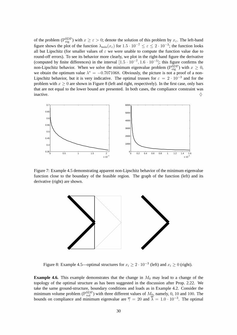
of the problem (PSDPeig ) with x ≥ ε > 0; denote the solution of this problem byxε. The left-hand

figure shows the plot of the functionλmin(xε) for 1.5 · 10−7 ≤ ε ≤ 2 · 10−3; the function looksall but Lipschitz (for smaller values ofε we were unable to compute the function value due toround-off errors). To see its behavior more clearly, we plotin the right-hand figure the derivative(computed by finite differences) in the interval[1.5 · 10−7, 1.6 · 10−5]; this figure confirms thenon-Lipschitz behavior. When we solve the minimum eigenvalue problem (PSDP

eig ) with x ≥ 0,we obtain the optimum valueλ∗ = −0.7071068. Obviously, the picture is not a proof of a non-Lipschitz behavior, but it is very indicative. The optimal trusses forε = 2 · 10−3 and for theproblem withx ≥ 0 are shown in Figure 8 (left and right, respectively). In the first case, only barsthat are not equal to the lower bound are presented. In both cases, the compliance constraint wasinactive. ♦

0 0.5 1 1.5 2

x 10−3

0.35

0.4

0.45

0.5

0.55

0.6

0.65

0.7

0 0.2 0.4 0.6 0.8 1 1.2 1.4 1.6

x 10−5

0

1000

2000

3000

4000

5000

6000

Figure 7: Example 4.5 demonstrating apparent non-Lipschitz behavior of the minimum eigenvaluefunction close to the boundary of the feasible region. The graph of the function (left) and itsderivative (right) are shown.

Figure 8: Example 4.5—optimal structures forxi ≥ 2 · 10−3 (left) andxi ≥ 0 (right).

Example 4.6. This example demonstrates that the change inM0 may lead to a change of thetopology of the optimal structure as has been suggested in the discussion after Prop. 2.22. Wetake the same ground-structure, boundary conditions and loads as in Example 4.2. Consider theminimum volume problem (PSDP

vol ) with three different values ofM0, namely,0, 10 and100. Thebounds on compliance and minimum eigenvalue areγ = 20 andλ = 1.0 · 10−3. The optimal

30

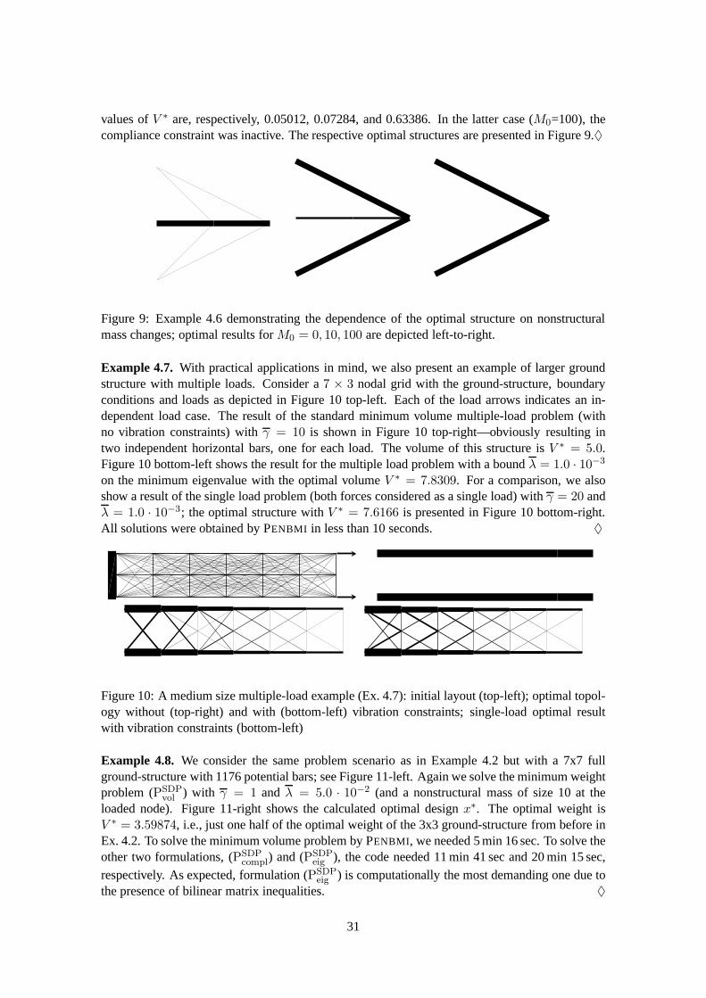
values ofV ∗ are, respectively, 0.05012, 0.07284, and 0.63386. In the latter case (M0=100), thecompliance constraint was inactive. The respective optimal structures are presented in Figure 9.♦

Figure 9: Example 4.6 demonstrating the dependence of the optimal structure on nonstructuralmass changes; optimal results forM0 = 0, 10, 100 are depicted left-to-right.

Example 4.7. With practical applications in mind, we also present an example of larger groundstructure with multiple loads. Consider a7 × 3 nodal grid with the ground-structure, boundaryconditions and loads as depicted in Figure 10 top-left. Eachof the load arrows indicates an in-dependent load case. The result of the standard minimum volume multiple-load problem (withno vibration constraints) withγ = 10 is shown in Figure 10 top-right—obviously resulting intwo independent horizontal bars, one for each load. The volume of this structure isV ∗ = 5.0.Figure 10 bottom-left shows the result for the multiple loadproblem with a boundλ = 1.0 · 10−3

on the minimum eigenvalue with the optimal volumeV ∗ = 7.8309. For a comparison, we alsoshow a result of the single load problem (both forces considered as a single load) withγ = 20 andλ = 1.0 · 10−3; the optimal structure withV ∗ = 7.6166 is presented in Figure 10 bottom-right.All solutions were obtained by PENBMI in less than 10 seconds. ♦

Figure 10: A medium size multiple-load example (Ex. 4.7): initial layout (top-left); optimal topol-ogy without (top-right) and with (bottom-left) vibration constraints; single-load optimal resultwith vibration constraints (bottom-left)

Example 4.8. We consider the same problem scenario as in Example 4.2 but with a 7x7 fullground-structure with 1176 potential bars; see Figure 11-left. Again we solve the minimum weightproblem (PSDP

vol ) with γ = 1 and λ = 5.0 · 10−2 (and a nonstructural mass of size 10 at theloaded node). Figure 11-right shows the calculated optimaldesignx∗. The optimal weight isV ∗ = 3.59874, i.e., just one half of the optimal weight of the 3x3 ground-structure from before inEx. 4.2. To solve the minimum volume problem by PENBMI, we needed 5 min 16 sec. To solve theother two formulations, (PSDP

compl) and (PSDPeig ), the code needed 11 min 41 sec and 20 min 15 sec,

respectively. As expected, formulation (PSDPeig ) is computationally the most demanding one due to

the presence of bilinear matrix inequalities. ♦

31

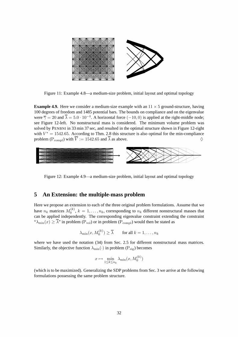
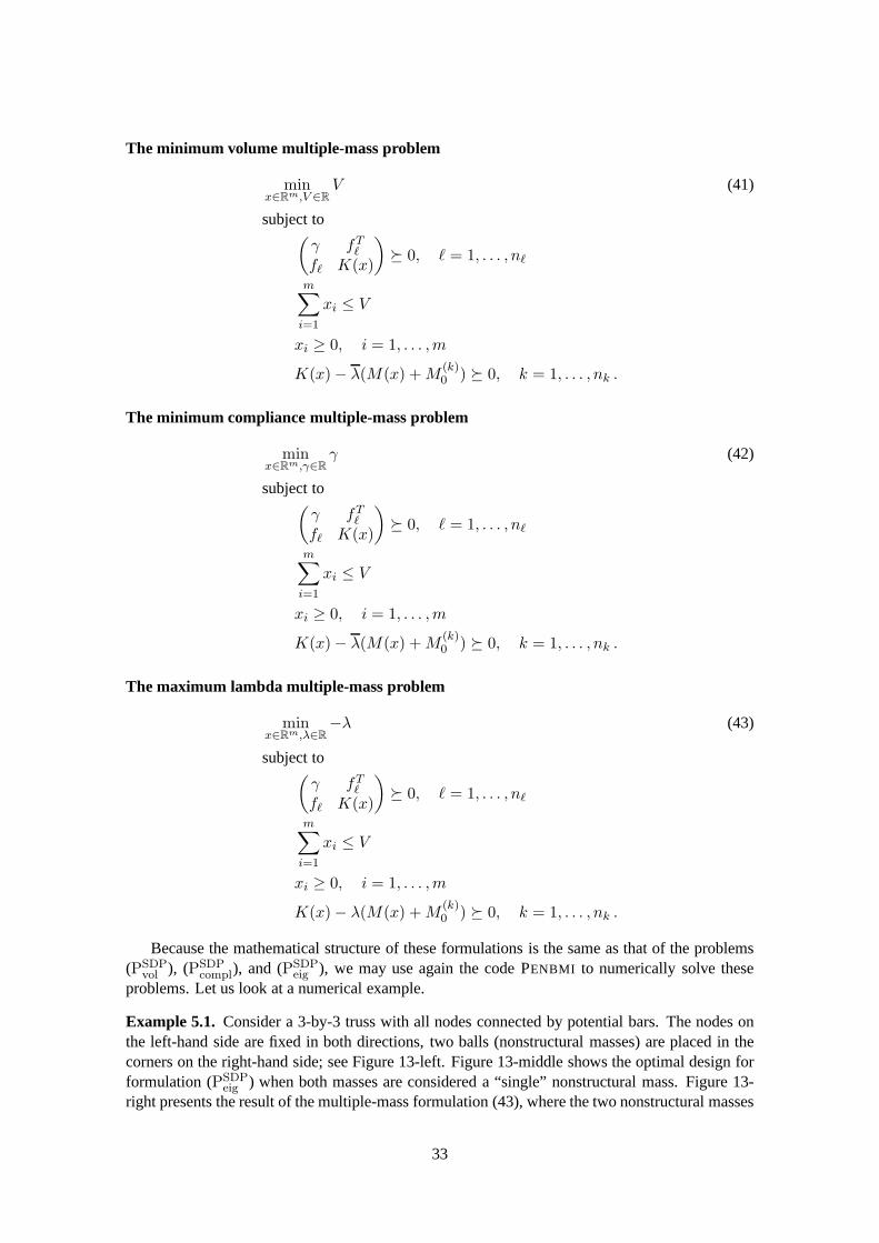
Figure 11: Example 4.8—a medium-size problem, initial layout and optimal topology

Example 4.9. Here we consider a medium-size example with an11 × 5 ground-structure, having100 degrees of freedom and 1485 potential bars. The bounds oncompliance and on the eigenvaluewereγ = 20 andλ = 5.0 · 10−4. A horizontal force(−10, 0) is applied at the right-middle node;see Figure 12-left. No nonstructural mass is considered. The minimum volume problem wassolved by PENBNI in 33 min 37 sec, and resulted in the optimal structure shown in Figure 12-rightwith V ∗ = 1542.65. According to Thm. 2.8 this structure is also optimal for themin-complianceproblem (Pcompl) with V := 1542.65 andλ as above. ♦

Figure 12: Example 4.9—a medium-size problem, initial layout and optimal topology

5 An Extension: the multiple-mass problem

Here we propose an extension to each of the three original problem formulations. Assume that wehavenk matricesM (k)

0 , k = 1, . . . , nk, corresponding tonk different nonstructural masses thatcan be applied independently. The corresponding eigenvalue constraint extending the constraint“λmin(x) ≥ λ” in problem (Pvol) or in problem (Pcompl) would then be stated as

λmin(x,M(k)0 ) ≥ λ for all k = 1, . . . , nk

where we have used the notation (34) from Sec. 2.5 for different nonstructural mass matrices.Similarly, the objective functionλmin(·) in problem (Peig) becomes

x 7→ min1≤k≤nk

λmin(x,M(k)0 )

(which is to be maximized). Generalizing the SDP problems from Sec. 3 we arrive at the followingformulations possessing the same problem structure.

32

The minimum volume multiple-mass problem

minx∈Rm,V ∈R

V (41)

subject to(

γ fTℓ

fℓ K(x)

)� 0, ℓ = 1, . . . , nℓ

m∑

i=1

xi ≤ V

xi ≥ 0, i = 1, . . . ,m

K(x) − λ(M(x) + M(k)0 ) � 0, k = 1, . . . , nk .

The minimum compliance multiple-mass problem

minx∈Rm,γ∈R

γ (42)

subject to(

γ fTℓ

fℓ K(x)

)� 0, ℓ = 1, . . . , nℓ

m∑

i=1

xi ≤ V

xi ≥ 0, i = 1, . . . ,m

K(x) − λ(M(x) + M(k)0 ) � 0, k = 1, . . . , nk .

The maximum lambda multiple-mass problem

minx∈Rm,λ∈R

−λ (43)

subject to(

γ fTℓ

fℓ K(x)

)� 0, ℓ = 1, . . . , nℓ

m∑

i=1

xi ≤ V

xi ≥ 0, i = 1, . . . ,m

K(x) − λ(M(x) + M(k)0 ) � 0, k = 1, . . . , nk .

Because the mathematical structure of these formulations is the same as that of the problems(PSDP

vol ), (PSDPcompl), and (PSDP

eig ), we may use again the code PENBMI to numerically solve theseproblems. Let us look at a numerical example.

Example 5.1. Consider a 3-by-3 truss with all nodes connected by potential bars. The nodes onthe left-hand side are fixed in both directions, two balls (nonstructural masses) are placed in thecorners on the right-hand side; see Figure 13-left. Figure 13-middle shows the optimal design forformulation (PSDP

eig ) when both masses are considered a “single” nonstructural mass. Figure 13-right presents the result of the multiple-mass formulation(43), where the two nonstructural masses

33

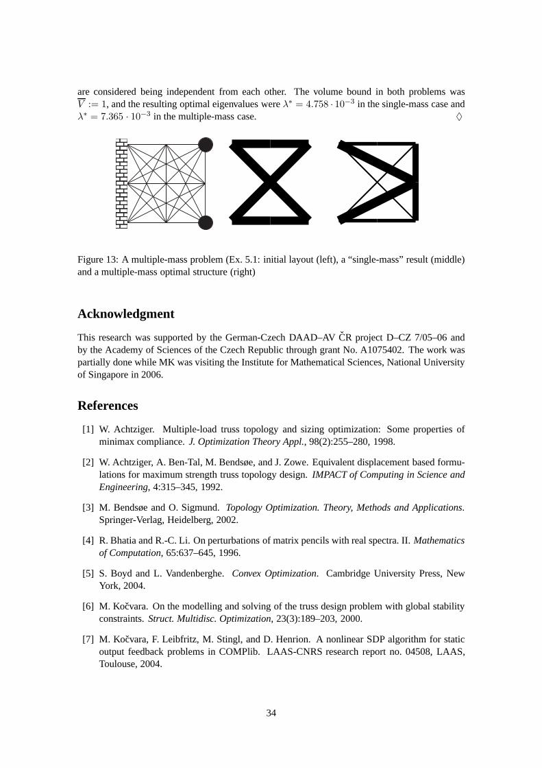
are considered being independent from each other. The volume bound in both problems wasV := 1, and the resulting optimal eigenvalues wereλ∗ = 4.758 · 10−3 in the single-mass case andλ∗ = 7.365 · 10−3 in the multiple-mass case. ♦

Figure 13: A multiple-mass problem (Ex. 5.1: initial layout(left), a “single-mass” result (middle)and a multiple-mass optimal structure (right)

Acknowledgment

This research was supported by the German-Czech DAAD–AVCR project D–CZ 7/05–06 andby the Academy of Sciences of the Czech Republic through grant No. A1075402. The work waspartially done while MK was visiting the Institute for Mathematical Sciences, National Universityof Singapore in 2006.

References

[1] W. Achtziger. Multiple-load truss topology and sizing optimization: Some properties ofminimax compliance.J. Optimization Theory Appl., 98(2):255–280, 1998.

[2] W. Achtziger, A. Ben-Tal, M. Bendsøe, and J. Zowe. Equivalent displacement based formu-lations for maximum strength truss topology design.IMPACT of Computing in Science andEngineering, 4:315–345, 1992.

[3] M. Bendsøe and O. Sigmund.Topology Optimization. Theory, Methods and Applications.Springer-Verlag, Heidelberg, 2002.

[4] R. Bhatia and R.-C. Li. On perturbations of matrix pencils with real spectra. II.Mathematicsof Computation, 65:637–645, 1996.

[5] S. Boyd and L. Vandenberghe.Convex Optimization. Cambridge University Press, NewYork, 2004.

[6] M. Kocvara. On the modelling and solving of the truss design problem with global stabilityconstraints.Struct. Multidisc. Optimization, 23(3):189–203, 2000.

[7] M. Kocvara, F. Leibfritz, M. Stingl, and D. Henrion. A nonlinear SDP algorithm for staticoutput feedback problems in COMPlib. LAAS-CNRS research report no. 04508, LAAS,Toulouse, 2004.

34

[8] M. Kocvara and J. Outrata. Effective reformulations ofthe truss topology design problem.Optimization and Engineering, 2005. In print.

[9] M. Kocvara and M. Stingl. PENNON—a code for convex nonlinear and semidefinite pro-gramming.Optimization Methods and Software, 18(3):317–333, 2003.

[10] M. Kocvara and M. Stingl. PENBMI User’s Guide. Version2.0., March 2005.http://www.penopt.com/ .

[11] A. S. Lewis and M. L. Overton. Eigenvalue optimization.Acta Numerica, 5:149–190, 1996.

[12] J. Lofberg. YALMIP : A toolbox for modeling and optimization in MATLAB.In Proceedings of the CACSD Conference, Taipei, Taiwan, 2004. Available fromhttp://control.ee.ethz.ch/˜joloef/yalmip.php .

[13] D. Luenberger.Optimization by vector space methods. J. Wiley and Sons, 1997.

[14] M. Ohsaki, K. Fujisawa, N. Katoh, and Y. Kanno. Semi-definite programming for topologyoptimization of trusses under multiple eigenvalue constraints. Comp. Meth. Appl. Mech.Engng., 180:203–217, 1999.

[15] N. Olhoff. Optimal design with respect to structural eigenvalues. In F.P.J. Rimrott andB. Tabarott, editors,Theoretical and Applied Mechanics, Proc. XVth Int. IUTAM Congress,pages 133–149. North-Holland, 1980.

[16] N. Olhoff and S. H. Rasmussen. On single and bimodal optimum bukling loads of clampedcolumns.Int. J. Solids Struct., 13:605–614, 1977.

[17] A. P. Seyranian and A. A. Mailybaev.Multiparameter stability theory with mechanical ap-plications. World Scientific, Singapore, 2003.

[18] G. W. Stewart. Perturbation bounds for the definite generalized eigenvalue problem.LinearAlgebra Appl., 23:69–86, 1979.

[19] M. Stingl. On the Solution of Nonlinear Semidefinite Programs by Augmented LagrangianMethods. PhD thesis, Inst. of Appl. Math., University of Erlangen, 2005.

[20] T. Zhang, K. H. Law, and G. H. Golub. On the homotopy method for perturbed symmetricgeneralized eigenvalue problems.SIAM J. Sci. Comput., 19:1625–1645, 1998.

A Appendix

Let x ∈ X be given and, for simplicity of notation, assume thatM0 = 0 (in general, we wouldassume thatker(M(x)) ⊂ ker(M0)). We want to show thatM(x) can be partitioned into

M(x) =

(MAA 0

0 0

)

whereMAA ≻ 0.

Lemma A.1. Let Zi ∈ Rn×n, Zi ≻ 0, andPi ∈ R

k×n, k < n, for i = 1, . . . , µ. Then, for anyz 6= 0,

µ∑

i=1

PiZiPTi z = 0 =⇒

µ∑

i=1

PiPTi z = 0 .

35

Proof. From the assumption we know thatµ∑

i=1zT PiZiP

Ti z = 0 andzT PiZiP

Ti z ≥ 0 for eachi

(asPiZiPTi � 0). ThuszT PiZiP

Ti z = 0 for all i and therefore‖Z1/2P T

i z‖22 = 0. As Z1/2 ≻ 0,

this immediately givesP Ti z = 0 ∀i, and the lemma follows.

Now letI includes the indices of all nonzero componentsxi of x. Without loss of generality,let us assume that the nonzero components ofx are equal to one, i.e.,xi = 1 for i ∈ I. Hence

M =m∑

i=1xiPiMiP

Ti =

∑i∈I

PiMiPTi . Define the projection

S = In×n −∏

i∈I

(In×n − PiPTi ) ;

clearly,S projects a vectorz ∈ Rn to a subspace generated by Euclidean unit vectors associated

with all degrees of freedom belonging to elementsi ∈ I, i.e., to the spacespan {PiPTi e, i ∈ I},

wheree ∈ Rn is the vector of all ones. From this definition, and from the construction ofM , weimmediately have thatM = SMS. Without loss of generality, assume thatS is of the form

S =

(Ik×k 0

0 0

)

wherek is the rank ofS. HenceM also has the form

M =

(M 00 0

)

with M ∈ Rk×k.

Lemma A.2. M is positive definite.

Proof. Assume thatMz = 0 for somez 6= 0. We need to show thatMz = 0 only for z = 0,wherez includes the firstk components ofz. By definition,

Mz =∑

i∈I

PiMiPTi z = 0 .

From the above lemma, we have that∑

i∈I

PiPTi z = 0 .

Now, the matrix∑i∈I

PiPTi is of the same form asS andM, and its upper-left block consists of a

(full) positive diagonal. Hencez = 0.

36