INDIAN COUNCIL FOR RESEARCH ON INTERNATIONAL ECONOMIC RELATIONS

Working Paper No. 184

Structural Shift in Demand for Food:Projections for 2020

Surabhi Mittal

August 2006

CONTENTS

LIST OF TABLES ......................................................................................................iii

LIST OF FIGURES ....................................................................................................iii

APPENDIX TABLES .................................................................................................iv

ABSTRACT..................................................................................................................v

FOREWORD...............................................................................................................vi

1. INTRODUCTION................................................................................................1

2. DATA ....................................................................................................................2

3. CHANGE IN CONSUMPTION PATTERN .....................................................2

4. WHAT AFFECTS CEREAL CONSUMPTION?.............................................7

5. DEMAND ELASTICITY ..................................................................................10

6. DEMAND PROJECTIONS ..............................................................................13

7. CONCERN FOR FOOD SECURITY..............................................................16

REFERENCES...........................................................................................................19

ANNEXURE ...............................................................................................................22

iii

LIST OF TABLES

Table 1: Households’ Budget Allocation to Food Across Different Expenditure Classes and Years..........................................................................................2

Table 2: Annual Per Capita Consumption .....................................................................4

Table 3: Stage Decomposition of Change in Cereal Consumption, 1983-99 ................9

Table 4: Estimated Food Expenditure Function, India (NSS consumer expenditure rounds for the years 1983, 1987, 1993 and 1999).......................................10

Table 5: Estimated Parameters of the Quadratic AIDS Food Demand System, India (NSS consumer expenditure rounds for the years 1983, 1987, 1993 and 1999) ...........................................................................................................11

Table 6: Expenditure Elasticity of Demand for Major Food Groups in India, 1999 ...12

Table 7: Own-price Elasticity of Demand for Major Food Groups in India, 1999 .....13

Table 8: Population Projection Figures........................................................................14

Table 9: Alternative Per Capita Income Assumptions for Demand Projections (%) ..14

Table 10: Projected Domestic Demand of Food Items in India under Alternative Scenarios .....................................................................................................15

Table 11: Projected annual per capita domestic demand of food items in India at GDP of 7 per cent.................................................................................................16

LIST OF FIGURES

Figure 1 : Change in budget share for food groups between 1983 and 1999 ................3

Figure 2: Annual Per Capita Consumption Across Year and Expenditure Classes for Cereals...........................................................................................................4

Figure 3: Annual Per Capita Consumption Across Year and Expenditure Classes for Vegetables and Fruits....................................................................................5

Figure 4: Annual Per Capita Consumption Across Year and Expenditure Classes for MFE ..............................................................................................................5

Figure 5 : Annual Per Capita Consumption Across Year and Expenditure Classes for Milk ...............................................................................................................5

Figure 6: Projected Foodgrain Availability and Demand in India...............................17

iv

APPENDIX TABLES

Table A 1: Budget Shares (per cent) of Different Expenditure Groups in 1983 .........27

Table A 2: Budget shares (per cent) of different expenditure groups in 1987 ............28

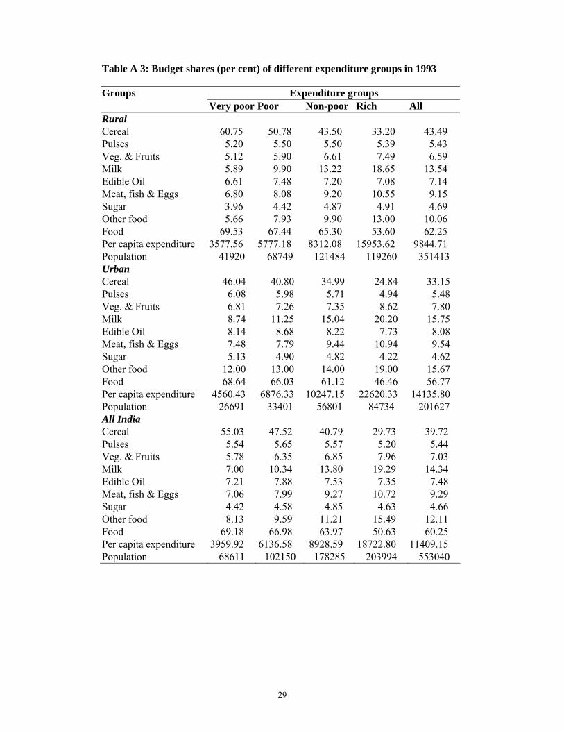
Table A 3: Budget shares (per cent) of different expenditure groups in 1993 ............29

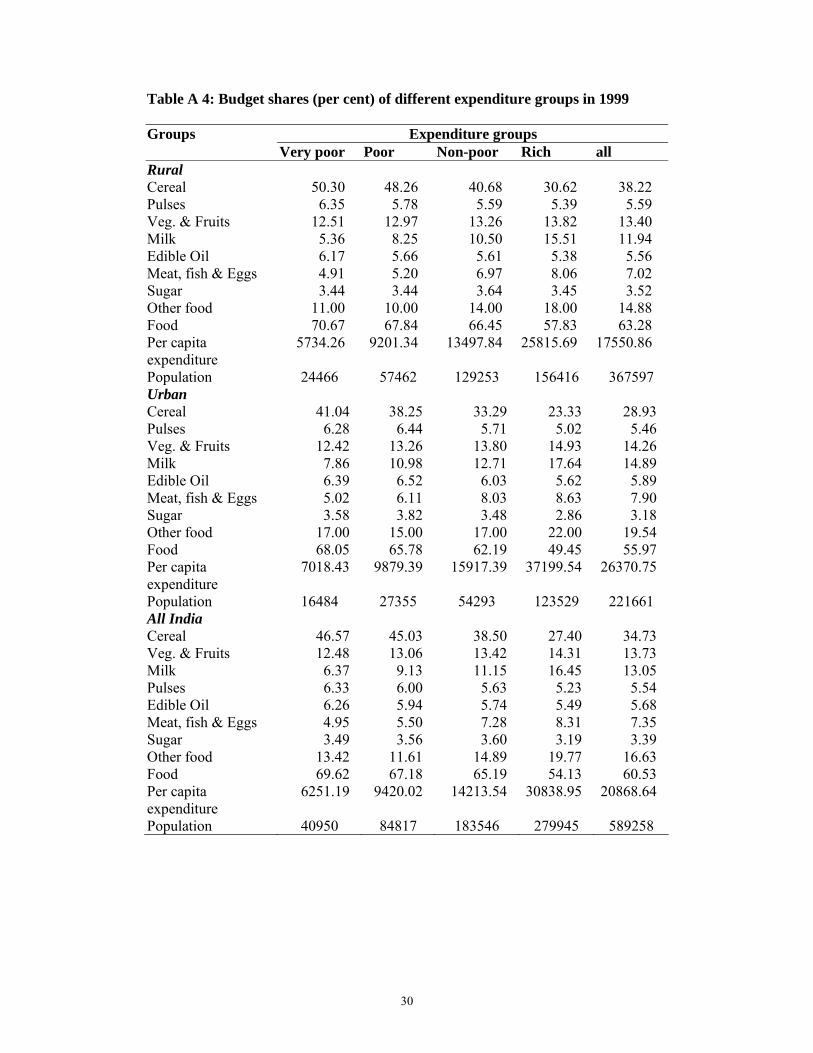
Table A 4: Budget shares (per cent) of different expenditure groups in 1999 ............30

Table A 5: Price of Food Items Paid by Consumers...................................................31

Table A 6: Annual per capita consumption of commodities across years and expenditure classes......................................................................................32

Table A 7: Expenditure elasticity of demand for major food groups in India, 1999...33

Table A 8: Own-price elasticity of demand for major food groups in India, 1999 .....33

Table A 9: Price elasticity of demand for major food groups in India, 1999 ..............34

Table A 10: Coefficients of estimated two-stage QUAIDS model..............................35

v

ABSTRACT

Knowledge of demand structure and consumer behaviour is essential for a wide range of development policy questions like improvement in nutritional status, food subsidy, sectoral and macroeconomic policy analysis, etc. An analysis of food consumption patterns and how they are likely to shift with changes in income and relative price is required to assess the food security-related policy issues in the agricultural sector. With high growth rates in the agricultural sector, the average per capita income in the country shows an increase, accompanied by a fall in the per capita consumption of staple food. In this background the present study diagnoses the food basket of households in rural and urban areas under different expenditure groups in the last two decades and tries to investigate the driving force for these changes by computing the demand elasticities that explain the level of demand for the commodities by an individual consumer given the structure of relative prices faced, real income and a set of individual characteristics such as age, type of household (expenditure groups) and geographical environment (rural or urban). The study projects the prospects of the food demand scenario in the country in 2020. And, finally, aims at finding answers to some of the most debatable issues relating to the country’s food security, decline in cereal consumption and implications on poverty. The study uses data from the consumer expenditure survey of the National Sample Survey (NSS) rounds number 38, 43, 50 and 55 Key Words: Household Food Consumption, Demand Elasticity, Decomposition, Demand Projections, Quadratic AIDS Model JEL Classification: Q11, Q18

vi

FOREWORD The issue of household food security has been one of the major concerns in India. There is an on-going debate on welfare implications of the decline in foodgrain consumption. Over the last two decades there appears to have been a structural shift in consumption pattern away from cereals to high-value agricultural commodities both in the urban and rural areas. From the available evidences it seems that even the very poor have tended to change their consumption pattern towards non-cereal commodities. This is perhaps a direct outcome of changes in relative prices over the years and an expected result of rise in per capita income levels. This study reviews past trends in per capita consumption of cereals and non- cereals using the NSS data on consumer expenditure to identify the factors that affect changes in cereal consumption. The paper then computes the demand elasticities for different food groups and makes demand projections for the year 2020 under different GDP scenarios. The demand elasticity and share of consumption expenditure on different food groups in total budget that are estimated in this paper provide the necessary criterion for various policy initiatives in this area. I hope that the findings reported here will provide an empirical basis for the on going discussion on agricultural diversification and changes in consumption pattern.

Rajiv Kumar Director and Chief Executive

ICRIER August 30, 2006

1

Structural Shift in Demand for Food: India’s Prospects in 20201

1. INTRODUCTION

Knowledge of demand structure and consumer behaviour is essential for a wide range of development policy questions like improvement in nutritional status, food subsidy, sectoral and macroeconomic policy analysis, etc. An analysis of food consumption patterns and how they are likely to shift as a result of changes in income and relative price is required to assess the food security-related policy issues in the agricultural sector. This analysis is based on a matrix of price and income elasticity of demand for food groups. In the short run, with relatively inflexible production, changes in the structure of demand are the main determinants of observed changes in market prices for non-tradable goods and of imports and exports of tradable goods. In medium and long runs, the structure of final demand is an important element of more complete models that seek to explain the levels of production and consumption, price formulation, trade flows, income levels and government fiscal revenues. With high growth rates in the agricultural sector, average per capita income in the country shows an increase. This is accompanied by a fall in the per capita consumption of staple food. This decline indicates improvement in the welfare, as laid down by Engel’s hypothesis. Kumar (1997) has pointed out that diversification in the food basket due to urbanization will provide food security and improve the quality of life by adding to the nutritional status and welfare of the population. With diversification, consumers are exposed to a wider choice of foods and shifts in dietary pattern either due to a rise in income or fall in price. Per capita consumption of foodgrains has been declining and some of this decline indicates an increase in the consumer’s welfare (Rao, 2000). Radhakrishna (2005) has argued that this sharp decline in cereal consumption can be attributed to changes in consumer tastes--from food to non-food items and, within the food group, from cereals to non-cereal food items and from ‘coarse’ to ‘fine’ cereals. These issues are generally debated as having a direct implication on poverty and increasing incidence of hunger in the country. Radhakrishna (2005) suggested that substantial expansion of the incomes of the poor is essential for tackling the chronic food insecurity problem. Debates on the issue of food security in terms of the country’s self-sufficiency in production, future demand for cereals and other food items as well as the ability of households to meet their calorie requirements are of important policy relevance. The present study diagnoses the food basket of households in rural and urban areas under different expenditure groups in the last two decades. The study investigates the factors that lead to these changes, computes demand elasticities that explain the level of demand for the commodities by an individual consumer given the structure of 1 Fellow, ICRIER; email: surabhi@icrier.res.in; mittal_surabhi75@yahoo.com

I would like to thank Prof. Praduman Kumar for providing me access to NSS data on consumer expenditure for all the four rounds used in the study. Consumer expenditure data of the next round could not be analysed by the time results for this study were finalised. I am grateful to Dr. Arvind Virmani, Prof. Praduman Kumar and Dr. Rajiv Kumar for their valuable comments and suggestions. I thank Mr. R. Srinivasulu for his research assistance.

2

relative prices faced, real incomes and a set of individual characteristics such as age, type of household (expenditure groups) and geographical environment (rural or urban). On this basis the study projects the country’s food demand scenario in 2020. And, finally, aims at finding answers to some of the debated issues relating to the country’s food security and decline in cereal consumption. 2. DATA

The National Sample Survey Organization (NSSO)2 collects data on household consumption expenditure at the national level in the form of various rounds by adopting sample survey techniques. The present study uses data from the consumer expenditure survey of the National Sample Survey (NSS) rounds number 38, 43, 50 and 55 pertaining to the periods 1983, 1987-8, 1993-4 and 1999-2000, respectively. These rounds provide household data in terms of quantity and value of commodities by expenditure groups, rural-urban locations and by states. The data are disaggregated with the level of individual crops, food and non-food items, total consumer expenditure and family size. The data refer to the average per capita consumption over the 30 day recall in each of the expenditure classes. Prices for rural and urban areas are computed implicitly as expenditure divided by the quantities of each of the expenditure classes in each round. For the purpose of analysis four expenditure groups are formed for both rural and urban households on the basis of the poverty lines adopted by the Planning Commission (Radhakrishna and Ravi 1990; Kumar 1998). Based on the expenditure groups of the NSS persons with expenditure below 75 per cent of the poverty line are defined as very poor; those between 75 per cent and the poverty line as poor; those at 150 per cent of the poverty line are termed as non-poor and those above 150 per cent of the poverty line are considered rich. 3. CHANGE IN CONSUMPTION PATTERN

The share of food in the total budget expenditure of a household has been showing a decline over the years, from 71.13 per cent in 1983 to 60.53 per cent in 1999 (Table 1). Table 1: Households’ Budget Allocation to Food Across Different Expenditure Classes and Years

Budget Share (%) Expenditure groups 1983 1987 1993 1999

Very poor 79.35 77.09 69.18 69.62 Poor 75.72 75.41 66.98 67.18 Non-poor 72.67 72.69 63.97 65.19 Rich 59.23 56.94 50.63 54.13 All 71.13 68.32 60.25 60.53 2 An ideal set for measuring the structural shifts in food demand patterns would record foods

consumed, prices, income by source and standard demographic information for a large number of families before and after these families migrated from rural to urban areas. Since such data sets are not available, the best possible way is to look into the household surveys of NSSO (Kumar, 1998).

3

This feature is prominent across households in different expenditure groups over time. The lowest income households spend around two-third of their total expenditure on food, while this is about 50 per cent for the rich households. It is very well recognized in literature that an increase in per capita income is accompanied by a fall in per capita consumption of staple food. The evidence is presented in Figure 1. Figure 1 : Change in budget share for food groups between 1983 and 1999

0

1020

3040

50

6070

8090

100

Vpo

or_8

3

Vpo

or_9

9

Poor

_83

Poor

_99

Non

poor

_83

Non

poor

_99

Ric

h_83

Ric

h_99

Expenditure groups

Per

cent

Cereal Pulses Milk V&F MFE Ofood

In India, although cereal continues to be the important constituent of a household’s food basket, its share in the total budget is declining. In the consumption food basket high-value foods such as vegetables and fruits (V&F), milk, meat, fish and eggs(MFE)3 are receiving increasing importance. These food items are rich in protein, essential vitamins, minerals and micronutrients. The share of other food4 has also shown an increase. The annual per capita consumption5 of foodgrains has declined between 1983 and 2000. The per capita consumption of cereals declined by 16.26 per cent while the per capita consumption of pulses increased marginally (Table 2). The consumption of vegetables and fruits, milk,, meat, fish and eggs edible oil and sugar has shown an increase.

3 Egg Equivalent used is 1 egg = 40 gms, thus approximately 1kg = 25 eggs. 4 In Figure 1 ‘other food’ includes sugar, edible oil, salt, pan, beverages, spices, etc. In the rest of the

study, sugar and edible oil are shown as separate groups. 5 Annual per capita consumption levels of various food items for years 1983, 1987, 1993 and 1999 for

India are presented in Table 4. Stratification for these years across expenditure groups is presented in Appendix Table A5.

4

Table 2: Annual Per Capita Consumption

Annual per capita consumption(Kg)

Group

1983 1987 1993 1999

Change in last two decades

(%)

Cereal 140.29 138.67 123.02 120.67 -16.26

Pulses 10.14 10.27 8.11 10.55 3.89

Milk 39.04 48.37 40.68 62.19 37.22

Edible oil 4.10 4.74 4.65 8.71 52.93

V&F 44.27 56.36 36.32 72.92 39.29

MFE 4.69 5.13 4.94 6.19 24.23

Sugar 9.69 9.99 8.92 12.05 19.59

Other food 31.21 29.81 24.21 32.96 5.31

Note: V&F=Vegetables and fruits; MFE= Meat, fish and eggs. As the income of poor people rises, consumption of cereals decline. This is demonstrated graphically in Figure 2. During the last two decades, as households moved from a lower expenditure class to a higher expenditure class there was a decline in additional cereal consumption. Decline in cereal consumption is substituted with increased consumption of vegetables and fruits, milk and meat, fish and eggs. Figure 2: Annual Per Capita Consumption Across Year and Expenditure Classes for Cereals

110

120

130

140

150

160

Very poor Poor Non-poor Rich

Expenditure class

Kg

1983 1999

5

Figure 3: Annual Per Capita Consumption Across Year and Expenditure Classes for Vegetables and Fruits

30

40

50

60

70

80

Very poor Poor Non-poor Rich

Expenditure class

Kg

1983 1999

Consumption of fruits and vegetables shows a constant rise with increase in income level (Figure 3). For meat, fish and eggs (Figure 4) as the income level increases the consumption increases--the magnitude of increase being the largest for the rich households. In 1999 the increase in the consumption of meat, fish and eggs was also huge in the non-poor households. Even for milk a similar pattern is observed in Figure 5. Figure 4: Annual Per Capita Consumption Across Year and Expenditure Classes for MFE

0

5

10

Very poor Poor Non-poor RichExpenditure class

Kg

1983 1999

6

Figure 5 : Annual Per Capita Consumption Across Year and Expenditure Classes for Milk

10

20

30

40

50

60

70

80

90

Very poor Poor Non-poor RichExpenditure class

Kg

1983 1999

The structural shift in consumption pattern is on account of the consumption diversification effect because of easy access to supply, changed tastes and preferences and change in relative prices (Appendix Table A5) (Radhakrishna and Ravi 1992; Kumar 1998; Murthy 2000). Increasing urbanization and economic growth reduces per capita demand for cereals and increases the demand for non-cereal food items. Modernization of agriculture also bears a similar negative relationship with the per capita consumption of cereals. Mechanization of agricultural activities and improvement in infrastructure also contribute to reduction in energy requirement and thus less cereal consumption (Rao 2000). This reconciles with the arguments by Kumar and Mathur (1996) that the demand for food is not only influenced by income changes, but also by differences in urban and rural lifestyle, the development of a more advanced marketing system and occupational changes that are closely linked with increasing per capita income. Substitution of cereal consumption with milk, fruits and vegetables is visible not only in the rich strata but also in the poorer strata across years. Households’ tastes and preferences are showing a shift towards high-value commodities. The decline in calorie intake as a result of reduced cereal consumption is compensated by the intake of high-value food items which are rich in calories and micronutrients. Rao (2000) has shown that the decline in cereal consumption has been sharper in the rural areas where improvements in rural infrastructure made other food and non-food items available to the rural households. Rao further observes that a reduction in the intake of foodgrains on this account should not be taken as deterioration in human welfare. According to J.V. Meenakshi (1996) the shift in the dietary pattern away from cereal consumption to more expensive milk, poultry and meat products is a consistent change associated with economic growth the world over. Huang and Bouis (1996) illustrate that in the rapidly growing economies of Japan, Korea and Taiwan

7

direct per capita consumption of cereals as staple food has declined over the past three decades while consumption of meat, fish and dairy products has increased dramatically. They explain such a change in Asian food consumption as the result of change in income and prices. In the last two decades between 1983 and 1999, both in rural and urban regions, there has been a structural shift in consumption pattern away from cereals to high-value agricultural commodities. The rural-urban difference in the per capita expenditure was 37.5 per cent in 1983. This narrowed down to 33.4 per cent in 1999 (Appendix Tables A1-A4). Regarding the expenditure on food items, rural and urban households used to spend the most on cereals which, in 1983, constituted about 50-65 per cent but declined to about 40-50 per cent in 1999. After cereals the next most important components in rural and urban households’ consumption basket are vegetables, fruits, milk, meat, fish, eggs and other food items. The assumption by Srinivasan and Bardhan (1969) that the preference structures of rural and urban consumers in the same expenditure class are identical is not contradicted. 4. WHAT AFFECTS CEREAL CONSUMPTION?

The concern about the decline in cereal consumption by the very poor can be shown as misplaced in the light of the structural change in their consumption basket towards non-cereal commodities. The increase in per capita income and the decline in the prices of food items which are substitutes for cereals play a key role in this diversification even for very poor income groups. This section of the study tries to understand the factors that affect the consumption pattern and the magnitude and direction of these factors. The focus is on decomposing the factors affecting cereal consumption in rural and urban areas and also in the four different expenditure groups. A two-stage budgeting framework is used to model the consumption behaviour of households6. The model does away with the assumption of linearity in the expenditure function and assumes that there is a non-linear relationship between income and expenditure. Quadratic equation is used as a specific case to non-linear function. Since the model is quadratic in per capita expenditure it is named as the quad-AIDS model. The model is estimated separately for each expenditure class7 across rural and urban regions. Separate coefficients are generated for each expenditure group for the purpose of decomposition across each group. Coefficients are presented in Appendix Table A10. The price variables are significant at 1 per cent significance level, but in some cases income variables are not significant even at 10 per cent significance level. The decomposition model is estimated at two stages with the estimated equations:

6 Methodology explained in detail in the Annexure. 7 Four expenditure groups are formed for both rural and urban households on the basis of the poverty

lines adopted by the Planning Commission (Radhakrishna and Ravi 1990; Kumar 1998).

8

Stage 1—Estimated food expenditure function:

timeYiYLnPLnPLnMLn oioinff δββγγα +++++= 2121 )(ln)()()()( (Equation 1)

where M is the per capita food expenditure; Y is the per capita total expenditure (income); Pf is the household specific price index for food; Pnf is price index of non-food. Time is the time trend

The first variable explains the own price effect, the second variable the substitution price effect, and the third and fourth variables the income effect while the time trend variables illustrate the impact of taste and preferences. Stage 2—Estimated share equation:

( ) timeeIMLncI

MLncFPLnbaS iiij

iijii ++++= ∑ 210 )()(

(Equation 2) where FPi is the price of the ith items/groups; I is the Stone geometric price index; The parameters of the model (ai, bij, c0i, c1iand eik) were estimated using the QUAIDS model by imposing the homogeneity (degree zero in prices) and symmetry (cross-price effects are same across the good) and adding up (all the budget shares add up to one) restrictions as shown in Appendix Table A10. In the second-stage estimations the share equations are estimated jointly for all the food groups. The first variable here explains the price effect. Own-price and substitution-price effects are separated out from here. The second and third variables explain the income effect and time trend is taste and preferences. There are some factors which cannot be quantified in the total estimated change. These are urbanization, development of market infrastructure, demonstration effect, eating out, etc. The results are presented in Table 3. In stage 1 there is decomposition of factors affecting per capita budget expenditure on food. As expected own-price effect has a positive sign. As food became relatively cheaper the expenditure on food items increased. Substitution-price effect sign is negative. This implies that as non-food items become relatively cheaper than food items consumers tend to shift some part of their expenditure on food to non-food products. This effect is of nearly equal magnitude in the poorest and the richest groups of the society. Both these groups trade off food items for non-food items with the extra real income. The poorer groups tend to spend a little more on non-food necessities while the richer groups spend more on luxury non-food items. Income effect is positive for poor and very poor groups but negative for the two upper income groups. This is true for both rural and urban regions. The upper expenditure groups tend to shift away budget expenditure from food as their income levels increase. Taste and preferences play an important role in favour of expenditure on food items.

9

Table 3: Stage Decomposition of Change in Cereal Consumption, 1983-99 Ist Stage Decomposition

Decomposition of factors affecting budget expenditure on food

Expenditure groups

Own price effect

Substitutionprice effect

Income effect

Taste & preferences

Total estimated change in PKFE

Rural Very poor 0.21 -0.75 0.49 1.18 1.13 Poor 0.23 -0.21 0.27 1.22 1.51 Non-poor 0.19 -0.50 -0.28 1.24 0.65 Rich 0.18 -0.75 -0.70 1.06 -0.20 Urban Very poor 0.23 -0.73 0.52 1.18 1.20 Poor 0.26 -0.21 0.28 1.22 1.54 Non-poor 0.21 -0.49 -0.28 1.23 0.67 Rich 0.20 -0.77 -0.72 1.06 -0.22

2nd Stage Decomposition

Decomposition of factors affecting share of per capita cereal consumption

Expenditure groups

Own price effect

Substitutionprice effect

Income effect

Taste & preferences

Total estimated change in share of cereal consumption

Rural Very poor 0.21 -0.21 4.73 -0.10 4.62 Poor 0.23 -1.67 3.79 -0.08 2.27 Non-poor 0.12 -0.12 1.96 -0.06 1.89 Rich 0.10 -0.66 0.19 -0.04 -0.41 Urban Very poor 0.22 -0.22 4.91 -0.10 4.81 Poor 0.23 -1.62 3.87 -0.08 2.40 Non-poor 0.12 -0.12 1.95 -0.06 1.89 Rich 0.11 -0.63 0.19 -0.04 -0.38

In stage 2 the factors affecting share of per capita cereal in total food expenditure is decomposed into price effects, income effect and taste and preferences. Own price and substitution price have expected signs. Thus, as cereals become relatively more expensive than their substitutes, there is a shift away from cereal consumption. Income has a positive effect on the share of cereal consumption in expenditure groups, but the effect in the poorest sections is alarming. Thus an extra income will make them purchase more of cereals. Changing tastes and preferences has led to a decline in the share of cereal consumption in total food expenditure by all the expenditure groups but the magnitude is highest for the poorest group. This implies that with time preferences are shifting away from cereal consumption. In between 180’s and late 1990’s with the development of rural markets, these regions as well as

10

the poor section of the society have been exposed to the availability of various cereal substitutes at relatively cheaper prices, than in past years. Ravallion (1990) states that the positive correlation between food prices and poverty is not an income distribution effect. Rather it appears to be the result of covariant fluctuations between average consumption and food prices caused by other variables including food supply, bad agriculture year, lower rural living standards and increase in food prices (Rao 1998). In other words, rural poverty increase when foods prices rise because the rural average income declines. Thus, as incomes increased and non-cereal food items became relatively cheaper during the last few years, the consumption of high-value commodities increased. This can be viewed as a positive effect on the welfare of the very poor group since the addition of food items which were earlier considered luxury commodities for this group now resulted in diversification in its consumption bundle. 5. DEMAND ELASTICITY

For a macro purpose, demand elasticity is of great importance at country level to project future demand. In this context regressions were again done at aggregate income levels for rural and urban regions. Price and expenditure elasticity were computed at mean level for 1999. The estimated parameters of total food expenditure function are given in Table 4. The explanatory variables included in the model explain 97 per cent of the total variation in the food expenditure function. The coefficients of food and non-food price factors have a negative and significant effect on the total food expenditure and are as per expectation. Per capita total expenditure and its square term are positive. The square term of per capita food expenditure is not significantly different from zero. This implies that the relation between expenditure and income change may not be non-linear. The linear term of per capita total expenditure is positive and significant; indicating that the response of total food expenditure on income change is substantial. The family size variable is negative and Table 4: Estimated Food Expenditure Function, India (NSS consumer expenditure rounds for the years 1983, 1987, 1993 and 1999) Variable Regression

coefficient Standard

error t-Value

Intercept -143.876 1.441 -99.817 Ln (price index for food) -0.075 0.021 -3.547 Ln (price index for non-food) -0.630 0.019 -33.735 Ln (per capita total expenditure) 0.627 0.056 11.176 Ln (per capita total expenditure)2 0.007 0.005 1.421 Family size -0.028 0.007 -4.172 Urban dummy 0.051 0.008 6.259 Time trend 0.073 0.001 102.212 Adjusted R2 0.97 Number of observations 920

11

significant. This implies that with a member added into a family the per capita expenditure on food declines due to reallocation of resources. Urbanization has a positive impact on food expenditure. Time trend is positive and significant. The estimation of the parameters of the quadratic demand system of the food group--cereals, pulses, vegetables and fruits, milk, edible oil, sugar and meat, fish and eggs are given in Table 5. The squared terms of per capita expenditure on food are significant only for pulses and edible oil. Urbanization has a negative effect on cereals, pulses and sugar consumption. The consumption of vegetables and fruits, milk and edible oil increase with urbanization. The coefficient of own price is positive and highly significant on the share of food groups. Even when prices rise the households maintain the share of staple food in their food consumption basket. The time trend is negative and significant for cereal, pulses and sugar. This implies that across years the share of these commodities in total food expenditure declines, but the decline is marginal due to a small coefficient. Table 5: Estimated Parameters of the Quadratic AIDS Food Demand System, India (NSS consumer expenditure rounds for the years 1983, 1987, 1993 and 1999)

Groups Cereals Pulses V&F Milk Edible Oil

Sugar MFE

Intercept 7.5432 0.0420 -1.9183 0.4933 -0.3629 0.5471 -5.3445 (7.96) (0.16) (-6.67) (0.73) (-1.33) (2.64) Food price (Rs/kg) in logarithmic form Cereal 0.0907 -0.0260 0.0195 -0.1067 -0.0242 -0.0340 0.0807 (9.20) (-13.40) (6.88) (-17.83) (-11.81) (-22.02) Pulses -0.0260 0.0161 0.0048 0.0008 -0.0042 0.0003 0.0082 (-13.40) (6.04) (4.06) (0.35) (-2.09) (0.19) V&F 0.0195 0.0048 0.0081 -0.0073 0.0004 0.0037 -0.0293 (6.88) (4.06) (4.36) (-3.03) (0.34) (4.22) Milk -0.1067 0.0008 -0.0073 0.0751 0.0081 0.0161 0.0139 (-17.83) (0.35) (-3.03) (11.37) (3.26) (8.48) Edible oil -0.0242 -0.0042 0.0004 0.0081 0.0140 -0.0030 0.0090 (-11.81) (-2.09) (0.34) (3.26) (5.34) (-1.72) Sugar -0.0340 0.0003 0.0037 0.0161 -0.0030 0.0120 0.0048 (-22.02) (0.19) (4.22) (8.48) (-1.72) (5.11) MFE 0.0807 0.0082 -0.0293 0.0139 0.0090 0.0048 -0.0873 (12.29) (4.45) (-11.99) (2.77) (4.70) (3.52)

-0.5009 0.1633 0.0570 0.0246 0.1976 0.0223 0.0362Ln (per capita food expenditure) (-3.58) (6.17) (1.43) (0.25) (6.93) (1.02)

0.0295 -0.0229 -0.0041 0.0207 -0.0282 -0.0012 0.0062Ln (per capita food expenditure)2

(1.46) (-5.95) (-0.71) (1.47) (-6.82) (-0.38)

Urban dummy -0.1401 -0.0005 0.0157 0.0302 0.0165 -0.0002 0.0784 (-24.97) (-0.43) (9.62) (7.65) (13.69) (-0.24) Year -0.0029 -0.0001 0.0010 -0.0004 0.0000 -0.0003 0.0027 (-6.02) (-1.14) (6.64) (-1.13) (0.18) (-2.83) DW Statistics 1.3790 1.4376 2.1415 0.9570 1.6475 1.4828 Note: Figures in parenthesis are the t-value. V&F=Vegetables and fruits; MFE= Meat, fish and eggs.

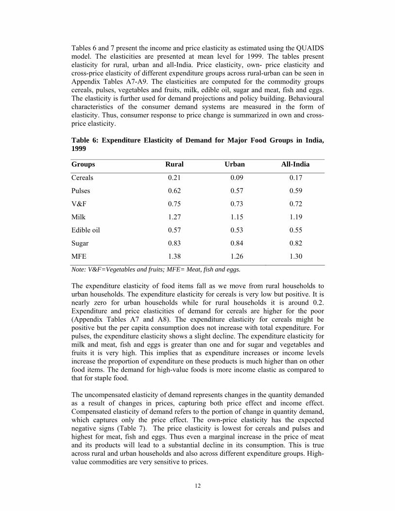
12

Tables 6 and 7 present the income and price elasticity as estimated using the QUAIDS model. The elasticities are presented at mean level for 1999. The tables present elasticity for rural, urban and all-India. Price elasticity, own- price elasticity and cross-price elasticity of different expenditure groups across rural-urban can be seen in Appendix Tables A7-A9. The elasticities are computed for the commodity groups cereals, pulses, vegetables and fruits, milk, edible oil, sugar and meat, fish and eggs. The elasticity is further used for demand projections and policy building. Behavioural characteristics of the consumer demand systems are measured in the form of elasticity. Thus, consumer response to price change is summarized in own and cross-price elasticity. Table 6: Expenditure Elasticity of Demand for Major Food Groups in India, 1999 Groups Rural Urban All-India

Cereals 0.21 0.09 0.17

Pulses 0.62 0.57 0.59

V&F 0.75 0.73 0.72

Milk 1.27 1.15 1.19

Edible oil 0.57 0.53 0.55

Sugar 0.83 0.84 0.82

MFE 1.38 1.26 1.30

Note: V&F=Vegetables and fruits; MFE= Meat, fish and eggs. The expenditure elasticity of food items fall as we move from rural households to urban households. The expenditure elasticity for cereals is very low but positive. It is nearly zero for urban households while for rural households it is around 0.2. Expenditure and price elasticities of demand for cereals are higher for the poor (Appendix Tables A7 and A8). The expenditure elasticity for cereals might be positive but the per capita consumption does not increase with total expenditure. For pulses, the expenditure elasticity shows a slight decline. The expenditure elasticity for milk and meat, fish and eggs is greater than one and for sugar and vegetables and fruits it is very high. This implies that as expenditure increases or income levels increase the proportion of expenditure on these products is much higher than on other food items. The demand for high-value foods is more income elastic as compared to that for staple food. The uncompensated elasticity of demand represents changes in the quantity demanded as a result of changes in prices, capturing both price effect and income effect. Compensated elasticity of demand refers to the portion of change in quantity demand, which captures only the price effect. The own-price elasticity has the expected negative signs (Table 7). The price elasticity is lowest for cereals and pulses and highest for meat, fish and eggs. Thus even a marginal increase in the price of meat and its products will lead to a substantial decline in its consumption. This is true across rural and urban households and also across different expenditure groups. High-value commodities are very sensitive to prices.

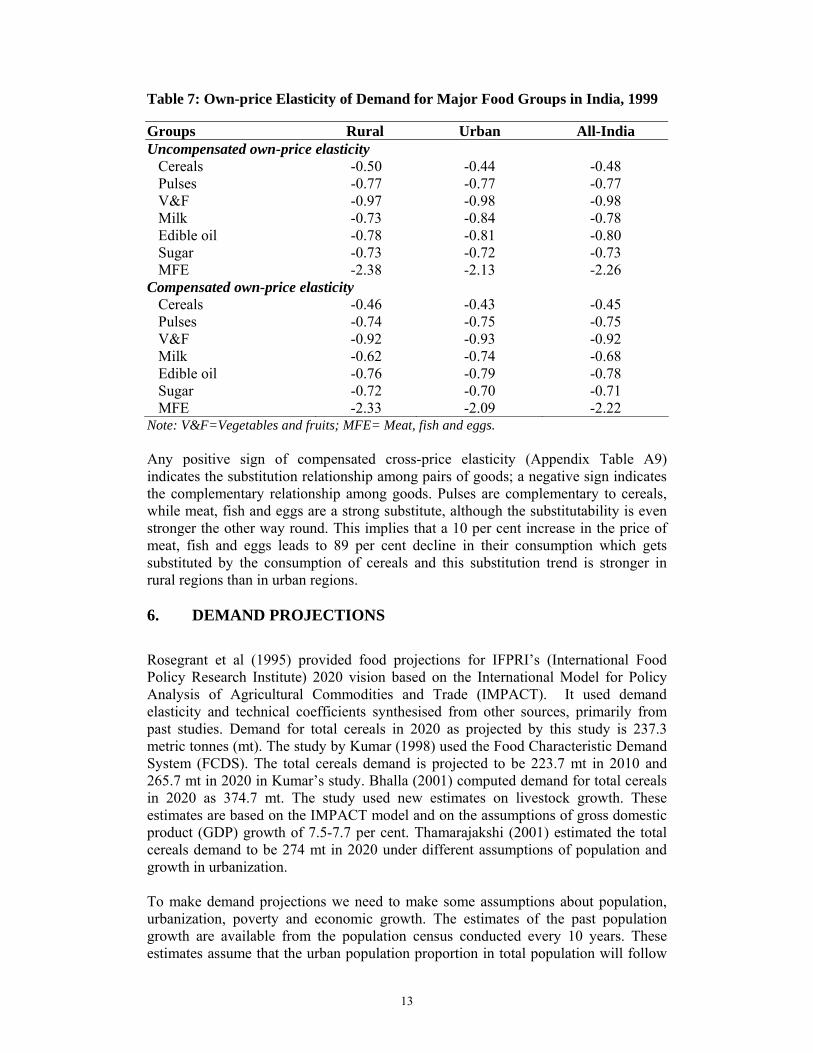
13

Table 7: Own-price Elasticity of Demand for Major Food Groups in India, 1999 Groups Rural Urban All-India Uncompensated own-price elasticity

Cereals -0.50 -0.44 -0.48 Pulses -0.77 -0.77 -0.77 V&F -0.97 -0.98 -0.98 Milk -0.73 -0.84 -0.78 Edible oil -0.78 -0.81 -0.80 Sugar -0.73 -0.72 -0.73 MFE -2.38 -2.13 -2.26

Compensated own-price elasticity Cereals -0.46 -0.43 -0.45 Pulses -0.74 -0.75 -0.75 V&F -0.92 -0.93 -0.92 Milk -0.62 -0.74 -0.68 Edible oil -0.76 -0.79 -0.78 Sugar -0.72 -0.70 -0.71 MFE -2.33 -2.09 -2.22

Note: V&F=Vegetables and fruits; MFE= Meat, fish and eggs. Any positive sign of compensated cross-price elasticity (Appendix Table A9) indicates the substitution relationship among pairs of goods; a negative sign indicates the complementary relationship among goods. Pulses are complementary to cereals, while meat, fish and eggs are a strong substitute, although the substitutability is even stronger the other way round. This implies that a 10 per cent increase in the price of meat, fish and eggs leads to 89 per cent decline in their consumption which gets substituted by the consumption of cereals and this substitution trend is stronger in rural regions than in urban regions. 6. DEMAND PROJECTIONS

Rosegrant et al (1995) provided food projections for IFPRI’s (International Food Policy Research Institute) 2020 vision based on the International Model for Policy Analysis of Agricultural Commodities and Trade (IMPACT). It used demand elasticity and technical coefficients synthesised from other sources, primarily from past studies. Demand for total cereals in 2020 as projected by this study is 237.3 metric tonnes (mt). The study by Kumar (1998) used the Food Characteristic Demand System (FCDS). The total cereals demand is projected to be 223.7 mt in 2010 and 265.7 mt in 2020 in Kumar’s study. Bhalla (2001) computed demand for total cereals in 2020 as 374.7 mt. The study used new estimates on livestock growth. These estimates are based on the IMPACT model and on the assumptions of gross domestic product (GDP) growth of 7.5-7.7 per cent. Thamarajakshi (2001) estimated the total cereals demand to be 274 mt in 2020 under different assumptions of population and growth in urbanization. To make demand projections we need to make some assumptions about population, urbanization, poverty and economic growth. The estimates of the past population growth are available from the population census conducted every 10 years. These estimates assume that the urban population proportion in total population will follow

14

past trends. In the simulation, three scenarios of income growth rate in GDP, viz. 6, 7 and 8 per cent, were considered. The results of food demand predictions corresponding to the scenario of 7 per cent GDP are considered to be most likely in the future. Opening up of trade and various structural and economic reforms are likely to accelerate the growth process to even 8 per cent. Adjustment for domestic saving rates is also made. The assumptions are specified in Tables 8 and 9. Table 8: Population Projection Figures (Unit: Millions) Source 2000 2005 2010 2015 2020 Registrar General

1027.02 1094.10 (1.59)

1178.90 (1.50)

1263.50 (1.40)

1345.63** (1.27)

Note: ** Self computed; Figures in parenthesis are population growth rates. The growth rates in per capita income under alternative scenarios are worked out by subtracting the population growth from income growth after adjusting for saving rates. This is then used for projecting the per capita consumption of different food items. Table 9: Alternative Per Capita Income Assumptions for Demand Projections (%) Year Low Actual High 2000 2.87 3.68 4.40 2005 3.23 4.04 4.76 2010 3.32 4.13 4.85 2015 3.43 4.24 4.96 2020 3.56 4.37 5.09 Note: Population growth between the years 1991-2001 is 1.95%;

Saving rate used is 23.5 % of GDP as in 2003-4 (Economic Survey, 2005-6); Low= If GDP is 5%; Actual=If GDP is 5.8%; High= If GDP is 7%.

The demand projections for the commodities are obtained through

ttt eyNdD )*1(*0 +=

where Dt is household demand of a commodity in year t; d0 is per capita demand of the commodities in the base year, y is growth in per capita income; e is the expenditure elasticity of demand for the commodity; Nt is the projected population in year t.

The demand projections are made using the demand elasticities as derived from the QUAIDS model presented in section 5 of this study of the study. The domestic demand projections are arrived at by adding up the direct demand (human demand) and the indirect demand (seed, feed, industrial use and wastage8). The household food demand is primarily driven by growth in population, income and change in income distribution (Kumar 1997). Apart from foodgrains demand for human consumption, an important component is the indirect demand of foodgrains for livestock consumption. Increasing demand for livestock products will rapidly drive up the

8 Demand for seed, feed, industrial use and wastage as given by Kumar (1998).

15

domestic requirement for foodgrains. Feed requirement and other uses to human consumption are added up to get total domestic demand for cereals and pulses. Food demand has been forecasted for the years 2005, 2010, 2015 and 2020 at the constant price of 1999-2000. Table 10 presents demand projections at three scenarios. The growth in the demand for cereals and pulses is mainly due to population growth. The demand for livestock sector is also increasing and thus an additional demand for cereals and pulses is generated to meet the animal feed demand. The total foodgrain demand projected for 2010, if the economy grows at 7 per cent, is 194.3 mt, with a break-up of 175.5 mt of cereal demand and 18.8 mt of pulse demand. This demand is expected to rise at a rate of 2.1 per cent and 3.3 per cent, respectively, between 2010 and 2020. In 2020 the projected domestic demand is 215.7 mt and 27.2 mt for cereal and pulses, respectively. Increase in demand for pulses is also visible because, for the vegetarian population, it is a major source of protein and also price substitution effect is strong from meat, fish and eggs to pulses and milk. Demand for milk and horticultural (fruits Table 10: Projected Domestic Demand of Food Items in India under Alternative Scenarios

Domestic Demand (Million metric tonnes)

Annual Growth Rate (%)

Groups GDP (%)

Base year 2000

2005 2010 2015 2020 2000-10

2010-20

2000-20

6 142.2 155.5 172.4 190.0 208.6 1.95 1.92 1.957 142.7 157.1 175.5 195.0 215.7 2.09 2.08 2.11

Cereals

8 143.7 159.6 179.8 202.1 225.9 2.27 2.31 2.316 13.5 15.4 18.0 21.1 24.8 2.89 3.27 3.117 13.6 15.8 18.8 22.6 27.2 3.30 3.73 3.55

Pulses

8 13.8 16.2 19.8 24.3 29.9 3.69 4.19 3.986 76.5 89.6 109.0 133.1 163.1 3.61 4.11 3.907 76.9 92.2 115.4 145.0 182.9 4.15 4.71 4.47

V&F

8 77.3 94.5 121.4 156.4 202.2 4.62 5.24 4.976 66.0 82.1 107.9 142.9 191.3 5.03 5.89 5.517 66.7 86.0 118.3 164.1 229.9 5.91 6.87 6.44

Milk

8 67.2 89.6 128.3 185.2 270.2 6.68 7.73 7.276 9.1 10.4 12.3 14.5 17.2 3.07 3.44 3.297 9.1 10.6 12.8 15.5 18.8 3.48 3.89 3.72

Edible oil

8 9.2 10.8 13.3 16.4 20.3 3.83 4.29 4.106 12.7 15.0 18.6 23.1 28.8 3.90 4.48 4.237 12.7 15.5 19.8 25.4 32.7 4.51 5.15 4.87

Sugar

8 12.8 16.0 21.0 27.6 36.7 5.04 5.75 5.456 6.6 8.3 11.2 15.1 20.6 5.39 6.34 5.917 6.7 8.8 12.3 17.5 25.2 6.35 7.41 6.94

MFE

8 6.7 9.2 13.5 20.0 30.1 7.19 8.36 7.85Note: Domestic demand takes into account the demand for seed, feed, industrial use and

wastage as given by Kumar (1998); V&F=Vegetables and fruits; MFE= Meat, fish and eggs.

16

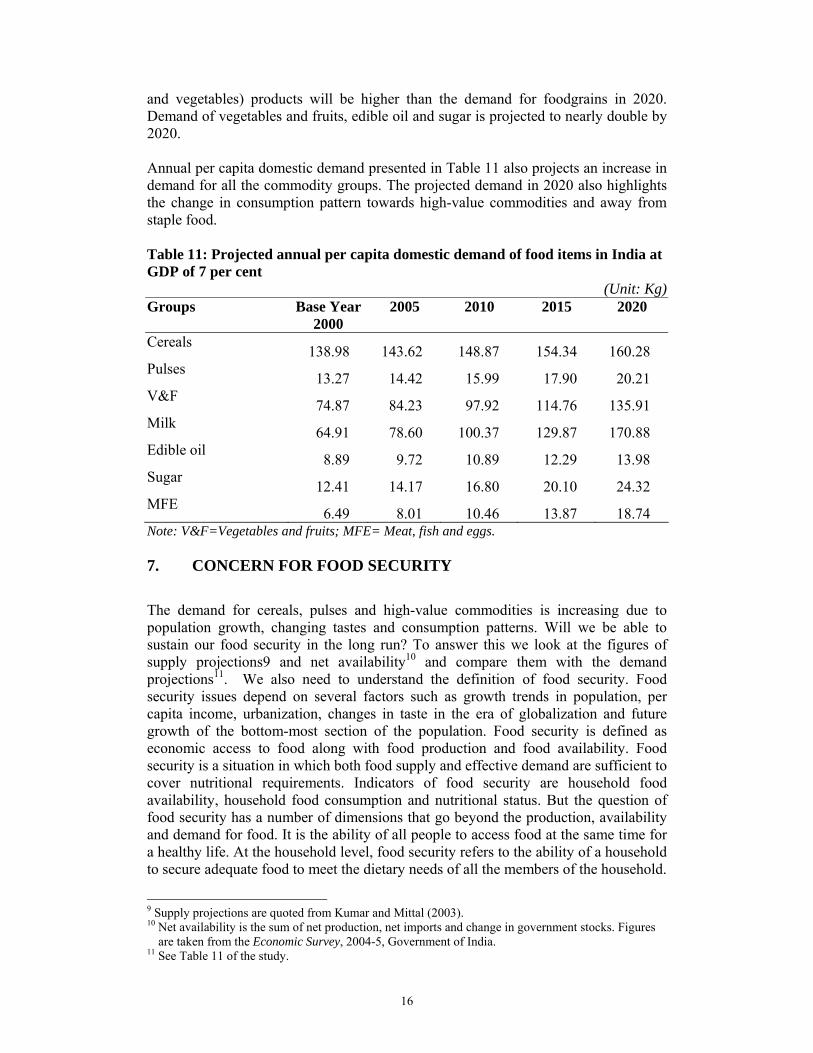
and vegetables) products will be higher than the demand for foodgrains in 2020. Demand of vegetables and fruits, edible oil and sugar is projected to nearly double by 2020. Annual per capita domestic demand presented in Table 11 also projects an increase in demand for all the commodity groups. The projected demand in 2020 also highlights the change in consumption pattern towards high-value commodities and away from staple food. Table 11: Projected annual per capita domestic demand of food items in India at GDP of 7 per cent

(Unit: Kg) Groups Base Year

2000 2005 2010 2015 2020

Cereals 138.98 143.62 148.87 154.34 160.28 Pulses 13.27 14.42 15.99 17.90 20.21 V&F 74.87 84.23 97.92 114.76 135.91 Milk 64.91 78.60 100.37 129.87 170.88 Edible oil 8.89 9.72 10.89 12.29 13.98 Sugar 12.41 14.17 16.80 20.10 24.32 MFE 6.49 8.01 10.46 13.87 18.74 Note: V&F=Vegetables and fruits; MFE= Meat, fish and eggs. 7. CONCERN FOR FOOD SECURITY

The demand for cereals, pulses and high-value commodities is increasing due to population growth, changing tastes and consumption patterns. Will we be able to sustain our food security in the long run? To answer this we look at the figures of supply projections9 and net availability10 and compare them with the demand projections11. We also need to understand the definition of food security. Food security issues depend on several factors such as growth trends in population, per capita income, urbanization, changes in taste in the era of globalization and future growth of the bottom-most section of the population. Food security is defined as economic access to food along with food production and food availability. Food security is a situation in which both food supply and effective demand are sufficient to cover nutritional requirements. Indicators of food security are household food availability, household food consumption and nutritional status. But the question of food security has a number of dimensions that go beyond the production, availability and demand for food. It is the ability of all people to access food at the same time for a healthy life. At the household level, food security refers to the ability of a household to secure adequate food to meet the dietary needs of all the members of the household.

9 Supply projections are quoted from Kumar and Mittal (2003). 10 Net availability is the sum of net production, net imports and change in government stocks. Figures

are taken from the Economic Survey, 2004-5, Government of India. 11 See Table 11 of the study.

17

Looking into the supply and demand balance for cereals, it appears that demand will be met in future with a surplus of cereals. Projected demand for cereals is 175.9 mt in 2010 and 216.7 mt in 2020, while the projected supply of cereals (Kumar and Mittal 2003) is 236.8 mt in 2010 and 274.0 mt in 2020. These figures are quite reassuring for the period up to 2020 for national food security. But when we talk about the issues of household food security then per capita net availability is a better measure. Figure 6 illustrates the per capita availability, per capita demand and per capita production projected12 for 2005, 2010, 2015 and 2020. The graph shows that the per Figure 6: Projected Foodgrain Availability and Demand in India

150

155

160

165

170

175

180

185

190

2000 2005 2010 2015 2020Year

Kg/

annu

m

PKAvail. PKDemand PKProd.

capita production will decline during the next two decades. But the per capita availability, which is net of stocks and trade, will take care of the increasing per capita demand of foodgrains in the country. However, if the per capita production shows a decline it remains an issue of concern. To improve food security at the national level we need to either increase agricultural production or increase imports. Since agricultural growth is limited, imports can act as a commercial means to improve the country’s food security. Primarily, for domestic agricultural growth we need to lay emphasis on productivity improvement, public investment in irrigation, infrastructure development, efficient use of water and plant nutrition. We also need to put in resources for research and development (Kumar 1998; Fan et al 1999; Evenson et al 1999). The scope of area expansion and livestock population increase is minimal; also some area has to shift from foodgrains to non-foodgrains to meet their increasing demand. While domestic production is still the most important source of food security, developing countries are gradually increasing their dependence on food imports. Thus, food security in developing countries will be boosted if they gain 12 These are forecasts based on the time series information available in the 2005 Economic Survey,

Government of India. The underlining assumption is that the past growth trend continues.

18

increased access to developed markets through trade liberalization (Trueblood and Shapouri 2001). Thus, these policies will help in maintaining yield growth that will enable the country to maintain a balance between domestic production and demand. Advances in crop production techniques in the post-green revolution period significantly helped in expanding food output and stocks of major cereals (rice and wheat) in India. This period also witnessed higher economic growth, population growth and increase in food demand. The shift in dietary patterns across regions and income classes is also observed. This brings a change in supply and demand prospects for food in the country in coming decades. Long-term food security demands that research in production technology of non-cereal food, through technology access to the poor small producers, should be promoted. Improvement in the quality of food items and reduction in transaction costs associated with their market access need to policy priorities. Thus a major challenge to household food security comes from the dietary diversification of the poor. On the production side, if cereal pricing is left to the market forces playing the facilitating role, land will be released from rice and wheat cultivation to meet the growing demand for non-cereal crops such as oilseeds, fruits and vegetables in accordance with diet diversification. This policy would facilitate agricultural diversification in tune with the emerging demand patterns. Higher value of future demand for these crops may justify extra research spending on crops whose demand will not respond strongly to rising urban incomes. The growing demand for livestock products gives an opportunity to increase incomes and employment and to reduce poverty in rural areas. If flexibility on the supply side is facilitated, production will adjust to the market forces and generate higher incomes in the rural areas.

19

REFERENCES

Ballino, Carlo (1990) ‘A Generalized Version of the Almost Ideal and Translog

Demand Systems’, Economics Letters, Vol. 34, Pp: 127-9. Barten, A.P. (1969) ‘Maximum Likelihood Estimation of a Complete System of

Demand Equations’, European Economic Review, Vol. 1, Pp: 7-73. Bhalla, G.S (2001). Demand and supply of food and feed grains by 2020 in the book

Towards Hunger Free India edited by M.D. Asthana and Pedro Medrano. New Delhi, Manohar.

Blundell, R., P. Pashardes and G. Weber (1993) ‘What Do We Learn about Consumer

Demand Pattern from Micro Data?’, American Economic Review, Vol. 83, Pp: 570-97.

Christensen, Laurits, Dale Jorgenson and Lawrence Lau (1975) ‘Transcendental Logarithmic Utility Functions’, American Economic Review, Vol. 65, Pp: 367-83.

Deaton, A.S. and J. Muellbauer (1980) ‘An Almost Ideal Demand System’, American

Economic Review, Vol. 70, Pp: 359-68. Deaton, Angus (1988) ‘Quality, Quantity and Spatial Variations of Prices’, American

Economic Review, Vol. 78, Pp: 418-30. Deaton, Angus (1989) ‘Household Survey Data and Pricing Policies in Developing

Countries’, World Bank Economic Review, Vol. 3, Pp: 183-210. Deaton, Angus (1990) ‘Price Elasticities from Survey Data: Extensions and

Indonesian Results’, Journal of Econometrics, Vol. 44, Pp: 281-309. Dey, Madan Mohan (2000) ‘Analysis of Demand for Fish in Bangladesh’,

Aquacultures, Economics and Management, Vol. 4, Pp: 63-81. Economic Survey (2004-5) Economics Division, Ministry of Finance, Government of

India. Evenson, R. E., C. Pray and M.W. Rosegrant (1999) ‘Agricultural Research and

Productivity Growth in India’, IFPRI Research Report No. 109, Washington, D.C.: International Food Policy Research Institute.

Fan, Shenggen, Peter Hazell and S. Thorat (1999) ‘Linkages between Government

Spending, Agricultural Growth and Poverty in Rural India’, IFPRI Research Report 110, Washington, D.C.: International Food Policy Research Institute.

Huang Jikun and Howarth Bouis (1996) ‘Structural Changes in the Demand for Food in Asia’, http://www.ifpri.org/2020/briefs/number41.htm

20

Kumar, Praduman (1997) ‘Food Security: Supply and Demand Perspective’, Indian Farming, December, Pp: 4-9.

Kumar, Praduman (1998) ‘Food Demand and Supply Projections for India’,

Agricultural Economics Policy Paper 98-01, New Delhi, India: Indian Agricultural Research Institute.

Kumar, Praduman (2004) ‘Fish Demand and Supply Projections in India’, ICAR-

ICLARM Project, Division of Agricultural Economics, New Delhi: Indian Agricultural Research Institute, March.

Kumar, Praduman and Surabhi Mittal (2003) ‘Productivity and Supply of Foodgrains

in India’, in A. Mahendra Dev, K.P. Kannan and Nira Ramchandran (eds) Towards a Food-secure India: Issues and Policies (2003), New Delhi: Institute for Human Development and Hyderabad: Centre for Economic and Social Studies.

Kumar, Praduman and V.C. Mathur (1996) ‘Structural Changes in Demand for Food

in India’, Indian Journal of Agricultural Economics, Vol. 51(4), Pp: 664-73.

Malthus, Thomas (1798) An Essay on the Principle of Population, London, printed for J. Johnson, in St. Paul's Church-Yard.

Meenakshi, J. V. (1996) ‘How Important are Changes in Taste: A State-level Analysis of Food Demand’, Economic and Political Weekly, 14 December, Pp: 3265-9.

Meenakshi, J.V. and R. Ray (1999) ‘Regional Differences in India’s Food

Expenditure Pattern: A Completed Demand Systems Approach’, Journal of International Development, Vol.11, Pp: 47-74.

Muellbauer, J. and P. Pashardes (1992) ‘Tests of Dynamic Specification and

Homogeneity in Demand Systems’, in L. Philips and L. D. Taylor (eds) Aggregation, Consumption and Trade: Essays in Honour of Hendrik Houthakker, Advanced Studies in Theoretical and Applied Econometrics, Kluwer Academic Publishers, Pp: 55-98.

Murthy, K.N. (2000) ‘Changes in Taste and Demand Pattern for Cereals’, Agricultural Economics Research Review, Vol.13 (1), Pp: 26-53.

Radhakrishna, R. and C. Ravi (1990) ‘Food Demand Projections for India’, Hyderabad: Centre for Economics and Social Studies.

Radhakrishna, R. and C. Ravi (1992) ‘Effects of Growth, Relative Price and

Preferences of Food and Nutrition’, Indian Economic Review, special number in memory of Sukhamoy Chakravarty, Vol. 27, Pp: 303-23.

Radhakrishna, R. and K. Venkata Reddy ‘Food security and Nutrition: Vision 2020’,

http://planningcommission.nic.in/reports/genrep/bkpap2020/16-bg2020.pdf Radhakrishna, R. (2005) ‘Food and Nutrition Security of the Poor’, Economic and

Political Weekly, Vol. XL, No.18, 30 April - 6 May, Pp: 1817-21.

21

Rao, C.H. Hanumantha (2000) ‘Declining Demand for Foodgrains in Rural India:

Causes and Implications’, Economic and Political Weekly, 22 January, Pp: 201-6.

Rao, J. Mohan (1998) ‘Food Prices and Rural Poverty: Liberalization without Pain’,

Economic and Political Weekly, Vol. 33(14), 4 April, Pp: 799-800. Ravallion, Martin (1990) ‘Income Effects on Undernutrition’, Economic

Development and Cultural Change, Vol. 38(3), University of Chicago Press, Pp: 489-515.

Rosegrant, M.W., M. Agcaoili-Sombilla and N.D. Perez (1995) ‘Global Food

Projections to 2020: Implications for Investment’, 2020 Discussion Paper No. 5, Washington, D.C.: International Food Policy Research Institute.

Sadoulet, Elisabeth and Alain de Janvry (1995) ‘Demand Analysis’, in Quantitative

Development Policy Analysis. Baltimore and London: The Johns Hopkins University Press.

Srinivasan, T. and P.K. Bardhan (1969) ‘Resources Prospects from the Rural Sector’,

Economic and Political Weekly, 28 June. Stone, Robert (1954) ‘Linear Expenditure System and Demand Analysis: An

Application to the Pattern of British Demand’, Economic Journal, Vol. 64, Pp: 511-27.

Thamarajakshi, R (2001). Demand and Supply of foodgrains in 2020 in the book

Towards HHHHHunger Free India edited by M.D. Asthana and Pedro Medrano. New Delhi, Manohar.

Theil, Henri (1976) ‘Theory and Measurement of Consumer Demand’, Amsterdam:

North-Holland.

Timmer, C. Peter (1991) ‘Agricultural Employment and Poverty Alleviation in Asia’, in C. P. Timmer (ed) Agriculture and the State: Growth, Employment, and Poverty in Developing Countries, Ithaca, NY: Cornell University Press, Pp: 123-55.

Trueblood, Michael and Shahla Shapouri (2001) ‘Implications of Trade Liberalization on Food Security of Low Income Countries’, Agriculture Information Bulletin No. 765-5, United States Department of Agriculture, Economic Research Services, April.

Zellner, A. (1962) ‘An Efficient Method of Estimating Seemingly Unrelated

Regressions and Tests for Aggregation Bias’, Journal of American Statistical Association. Vol. 57, Pp: 348-75.

22

ANNEXURE

METHODOLOGICAL NOTE ON DEMAND MODEL Methodologically, there are two approaches that can be followed to estimate the parameters of demand equations. One consists of specifying estimable single equation demand function in a pragmatic fashion without recourse to economic theory. A typical situation, for instance, is to estimate from time series data the income and price elasticities for a commodity in a constant elasticity demand equation. The use of relative prices and real income in the equation as exogenous variable makes the demand equations homogeneous of degree zero in prices and income. This ensures that there is no money illusion in demand in the sense that it is not affected by a proportional increase in all prices and incomes. This approach is simple but has serious drawbacks (Sadoulet and Janvry 1995). First, the choice of functional form for the demand equation in a single equation demand function and of variables to be included is arbitrary. The guidelines used are usually a combination of common sense, interest in specific elasticities, computational convenience and goodness of fit criteria. Second, this functional form postulates constancy of elasticities over all values of the exogenous variables. This can be true for only a short range of price and income for policy analysis. Typically, commodities that are luxuries (high-income elasticity) become necessitates (low-income elasticities) when per capita income increases. The third drawback is that the estimated parameters, in general, do not satisfy the requirements of demand theory, particularly the budget constraint. An alternative approach to the estimation of demand equation parameters uses the theory of demand as a guideline for the choice of functional forms and variables to be included. In particular, the theory allows the derivation of estimable functional forms of demand equations from mathematically specified models of consumer choice and imposition of constraints on demand parameters to reduce the number of independent parameters to be estimated to manageable numbers relative to data availability. Three demand systems have received considerable attention: the Linear Expenditure System (LES) developed by Stone (1954), the Almost Ideal Demand System (AIDS) developed by Deaton and Muellbauer (1980) and the combination of these two systems into a Generalized Almost Ideal Demand System (GAIDS) proposed by Ballino (1990). Other complete demand systems found in the literature but not widely used are the Rotterdam model of Theil (1976) and Barten (1969) and the translog model of Christensen, Jorgenson and Lau (1975). The Linear Expenditure System is the most frequently used system in empirical analysis of demand. A significant drawback of this system is that it implies linear Engel functions, a specification not supported by empiricism and can be true only over a short range of variation of income. Consequently, if the equations are to be used for predictions, only short-term predictions can be made. Like all point wise-separable models, the LES model is better applied to large categories of expenditure than to individual commodities, since it does not allow for inferior goods and implies that all goods are gross complements.

23

The AIDS model derives from a utility function specified as a second order approximation to any utility function. The demand functions are derived in budget share form. Deaton and Muellbauer (1980) suggest approximating the price index P by the Stone geometric price index:

ii

i pwP ln*ln ∑=

This linear approximation is all the better if there is collinearity in prices over time. The econometric problem with the AIDS model is that the demand equations appear to be unrelated, since none of the endogenous quantities or budget share appear on the right-hand side of the equations. This is not the case, however, since error terms across equations are correlated by the fact that the dependent variables need to satisfy the budget constraints. While an ordinary least squares (OLS) estimate of these equations would be consistent and unbiased, the estimation method developed by Zellner (1962) for Seemingly Unrelated Regressions (SUR) provides estimates that are more efficient. In a first stage, OLS is used to estimate the variance-covariance matrix residual; in a second stage this estimated matrix is used in a generalized least square estimation. Since the covariance matrix among residuals is singular because of the residuals satisfying the budget constraint, the typical procedure consists in deleting one of the equations of the demand system. The parameters from the deleted equation can be calculated from the parameters of the other equations through the restrictions on parameters. Barten (1969) has suggested an Iterated Seemingly Unrelated Regression (ITSUR) routine, which produces results that are invariant to the equation deleted. Demand parameters need to satisfy a number of exact restrictions and these must be imposed on the estimators. Equality constraints are imposed by using a restricted least square approach. The basic objective of the theory of consumer behaviour is to explain how a rational consumer chooses what to consume when confronted with various prices and a limited income. At this level of generality, the main usefulness of the theory for empirical purposes is that it establishes a set of constraints which demand parameters must satisfy, thus limiting the number of independent parameters to be estimated and ensuring consistency in the results obtained. Due to time series data constraint, we use recently developed techniques for estimating price elasticities using cross section expenditure survey data when there are spatial variations in prices. The data requirements to apply these techniques are household expenditures by commodity, quantity of each commodity consumed and individual characteristics. Given expenditure and quantity data, the unit value and expenditure shares can be calculated for each household. Consumers respond to price movements by changing both the quantity and quality of a good. Demand elasticities are an important parameter in predicting food demand. The magnitude of these elasticities depends largely on the methodology used in computing the price and expenditure elasticity. Different studies have used different methods to estimate the demand elasticities and make demand projections. Kumar (1998) computed the expenditure and price elasticities for food and non-food commodities using various econometric (Transcendental Logarithmic Demand System (TLDS), Normalized Quadratic Demand System (NQDS) and Linear Expenditure Demand

24

System (LEDS)) and non-econometric (Food Characteristic Demand System (FCDS)) techniques. More recent studies are centred around the complete demand system, which takes into account mutual interdependence of a number of commodities in the budget decisions of the consumer. Muellbauer and Pashardes (1992) point out that most studies of demand systems use static models, which did not account for hypothesis of symmetry and homogeneity, derived from consumer theory. Thus, there is a need for a dynamic demand system which gives more realistic and econometrically viable results. Demand and income elasticities are not necessarily constant across groups. Indeed, food income elasticities generally decrease with increasing income (Ravallion 1990; Timmer 1991). If this property is not allowed in the functional form, it inevitably results in bias. Similarly, if changes in relative prices are not accounted for then it can lead to omitted variable bias. The functional form used in the demand study affects estimates. There are two important requirements for the functional form that are used to estimate income elasticities13 of food demand. They should be flexible and allow income elasticities to differ between rich and poor households, because the usual pattern is of income elasticities of food demand to fall as income rises. The functional form should be able to be estimated when a household has zero consumption of particular foods, otherwise those households have to be dropped from the sample, which could cause sample selection bias (Deaton 1989) The present study works with the complete demand system and makes demand projections after taking into account urbanization, regional variations in dietary pattern and income distribution. Several studies in literature have shown that demand elasticities can vary across income groups and by regions as production environments and tastes change. If demand is analysed directly at the regional or national level, it is affected by both the averages level of these variables in the unit of analysis and by their distribution across the population. The Deaton (1988,1990) method assumes that there are no price variations within clusters and, hence, unit value variations across households in the same cluster are only due to quantity differentials and measurement errors. This assumption allows one to use within-cluster variations in demand to estimate the impact of income and consumer characteristics on demand including the quantity effects. This relation can then be used to remove the predicted effects of income and household characteristics on demand and to explain the residual cross-cluster variations in demand by prices only. The study estimated an extended model of the AIDS model. The model gives away the assumption of linearity in the expenditure function. The model assumes that there is a non-linear relationship between income and expenditure. Quadratic equation is used as a specific case to non-linear function. The model is quadratic in per capita 13 The income elasticity of demand measures the percentage by which the quantity demanded of an

item increases following 1 per cent increase in household income. When demand increases by more than 1 per cent an item is known as a luxury good, when the demand increases by between zero and 1 per cent it is a normal good and when the demand goes down as incomes rise, it is an inferior good.

25

expenditure thus the model is named as quad-AIDS model. A multi-stage (two-stage) budgeting framework is used to model the consumption behaviour of households. In the first stage, the household makes decisions on how much of its total income (expenditure) is to be allocated for food consumption, conditional on consumption of the non-food goods and the household and demographic characteristics. In the second stage, the household allocates the total food expenditure among different items/groups (rice, wheat, coarse cereals, pulses, milk, edible oils, vegetables, fruits, meat, fish, eggs, sugar, other food, and non-food). Following Blundell et al. (1993), Dey (2000) and Kumar (2004), the specific functional form used in the two stages are as follows: Stage 1: Food expenditure function

ZYYLnPLnPLnMLn jonff ∑+++++= θββγγα 2121 )(ln)()()()( (1)

Where M is the per capita food expenditure; Y is the per capita total expenditure (income); Pf is the household specific price index for food; Pnf is price index of non-food. Socio-demographic and conditioning variables (vector Z) include ratio of adults in the household, family size, and urban dummy. Equation 1 was estimated by the OLS method, and homogeneity of degree zero in prices and income was imposed by restricting γ1 + γ2+ β0 +2β1 Ln(Y) = 0 at the sample mean of Ln(Y). Stage 2: Quadratic-AIDS (QUAIDS) Model In stage 2 of the analysis, quadratic extension to Deaton and Muellbauer’s (1980) almost ideal model (QUAIDS) for food demand system will be used. This model is quite popular and was adopted recently by Meenakshi and Ray (1999) for India food model, Dey (2000) for fish demand model of Bangladesh and Kumar (2004) for fish demand model of India. The specific functional form for ith items/groups is as follows:

( ) kk

ikiiij

iijii IMReUrbandIMLncI

MLncFPLnbaS ∑∑ +++++= 210 )()(

(2) Where FPi is the price of ith items/groups; I is the Stone geometric price index; Urban is a binary dummy variable for urban areas. The parameters of the model (ai, bij, ci, di and eik) were estimated by imposing the homogeneity (degree zero in prices), symmetry (cross price effects are same across the good), and adding up (all the budget shares add up to one) restrictions. The following restrictions were econometrically imposed.

Homogeneity: ;0

1=∑

=

n

jijb

Symmetry: ,jiij bb = ;.....

0

1

20

21

10

11

n

nc

cc

cc

c ===

Adding up: ,1=∑ ia 00 === ∑∑∑i

ii

iji

i dbc

The homogeneity and symmetry restrictions are imposed at sample mean. Adding up restriction is imposed while computing the parameters of the last equation of the model, which is not included in the estimation. Given the quadratic specification of the demand system (Equations 1 and 2) a test of symmetry additionally requires that the ratio of the coefficients on the food expenditure and the square terms in food

26

expenditure be the same for all items/groups (Blundell et al 1993). The predicted value of food expenditure obtained from stage 1 will be used as the explanatory variable. The income and price elasticities can easily be computed as follows: Food income elasticity

1)/)(2( 10 ++= iiii wFLnccη Uncompensated price elasticity

iji

jii

i

ijij kw

wFLnccwb

−⎟⎠⎞

⎜⎝⎛+−⎟⎟

⎠

⎞⎜⎜⎝

⎛= ))(2( 10ξ

where kij is Kronecker delta, which takes the value of one for own-price elasticity and zero for cross-price elasticity; and wi is the share of the ith items/groups used as a weight in constructing Stone’s price index. Once the expenditure and uncompensated price elasticities are estimated, the compensated own and cross-price elasticities are computed using the Slutsky equation in elasticity form:

ijijH

ij w ηξξ +=

where H

ijξ is the compensated (Hicksian) price elasticity.

Income elasticity of demand for an individual items/groups <y

iη > was estimated as

the product of expenditure elasticity of the individual items/groups < iη > and food

expenditure elasticity with respect to total income (yη ):

yi

yi ηηη ×=

27

APPENDIX TABLES Table A 1: Budget Shares (per cent) of Different Expenditure Groups in 1983 Groups Expenditure Groups Very poor Poor Non-poor Rich All Rural Cereal 64.43 56.59 50.45 40.27 52.42 Pulses 4.38 5.12 5.10 5.39 5.01 Veg. & fruits 8.26 9.15 9.28 10.01 9.20 Milk 5.01 8.01 11.10 15.52 10.14 Edible oil 4.78 5.71 5.67 6.00 5.56 Meat, fish & eggs 3.79 4.21 5.46 6.83 5.15 Sugar 3.29 3.88 4.14 4.56 4.00 Other food 6.06 7.34 8.80 11.00 8.41 Food 80.15 76.49 73.99 61.28 72.80 Per capita expenditure 1411.42 2097.24 2915.85 5502.51 3033.96 Population 88301 87821 124219 97307 397648 Urban Cereal 50.96 44.14 36.48 27.09 37.83 Pulses 5.42 5.20 5.34 4.91 5.19 Veg. & fruits 8.94 9.88 10.84 12.70 10.87 Milk 8.04 10.30 13.18 16.95 12.81 Edible oil 6.82 7.41 7.60 7.54 7.39 Meat, fish & eggs 5.18 6.31 7.64 8.75 7.25 Sugar 4.11 4.40 4.14 3.88 4.10 Other food 11.00 12.00 15.00 18.00 14.58 Food 77.50 73.93 69.76 56.02 67.72 Per capita expenditure 1923.92 2914.87 4108.45 8526.43 4852.03 Population 38174 38088 56611 61957 194830 All-India Cereal 60.37 52.82 46.08 35.14 47.62 Pulses 4.70 5.14 5.17 5.20 5.07 Veg. & fruits 8.46 9.37 9.77 11.06 9.75 Milk 5.93 8.70 11.75 16.07 11.02 Edible oil 5.40 6.22 6.28 6.60 6.16 Meat, fish & eggs 4.21 4.85 6.14 7.58 5.84 Sugar 3.53 4.04 4.14 4.30 4.03 Other food 7.55 8.75 10.74 13.72 10.44 Food 79.35 75.72 72.67 59.23 71.13 Per capita expenditure 1566.11 2344.58 3289.21 6678.88 3631.81 Population 126475 125909 180830 159264 592478

28

Table A 2: Budget shares (per cent) of different expenditure groups in 1987

Expenditure groups Groups Very poor Poor Non-poor Rich All

Rural Cereal 54.47 47.54 40.95 31.31 40.80 Pulses 4.74 5.31 5.33 5.39 5.27 Veg. & Fruits 10.74 10.91 10.85 11.65 11.12 Milk 5.36 8.23 11.78 16.49 11.81 Edible Oil 5.96 6.81 7.09 7.35 6.97 Meat, fish & Eggs 5.74 6.51 7.68 8.65 7.52 Sugar 3.69 3.99 4.17 4.44 4.16 Other food 9.29 11.00 12.00 15.00 12.45 Food 78.20 76.60 74.18 59.36 70.17 Per capita expenditure 2128.99 3212.83 4484.73 9217.47 5521.16 Population 59607 87030 145166 149756 441559 Urban Cereal 40.67 36.32 31.37 21.28 30.04 Pulses 5.75 5.97 5.63 4.94 5.45 Veg. & Fruits 12.37 11.90 12.68 14.06 13.00 Milk 8.25 11.09 13.91 17.89 13.94 Edible Oil 8.57 8.73 8.75 8.41 8.59 Meat, fish & Eggs 6.14 6.71 8.07 9.72 8.12 Sugar 4.59 4.36 4.09 3.57 4.03 Other food 14.00 15.00 16.00 20.00 16.99 Food 75.27 72.74 68.96 52.46 64.49 Per capita expenditure 2527.48 3828.65 5735.46 13093.77 7621.84 Population 36369 38736 58176 80767 214048 All India Cereal 49.24 44.08 38.21 27.80 37.29 Pulses 5.12 5.52 5.41 5.23 5.33 Veg. & Fruits 11.36 11.21 11.37 12.49 11.73 Milk 6.46 9.11 12.39 16.98 12.51 Edible Oil 6.95 7.40 7.56 7.72 7.50 Meat, fish & Eggs 5.89 6.57 7.79 9.02 7.71 Sugar 4.03 4.10 4.15 4.14 4.12 Other food 11.07 12.23 13.14 16.75 13.93 Food 77.09 75.41 72.69 56.94 68.32 Per capita expenditure 2279.99 3402.50 4842.56 10515.59 6207.01 Population 95976 125766 203342 230523 655607

29

Table A 3: Budget shares (per cent) of different expenditure groups in 1993

Expenditure groups Groups Very poor Poor Non-poor Rich All

Rural Cereal 60.75 50.78 43.50 33.20 43.49 Pulses 5.20 5.50 5.50 5.39 5.43 Veg. & Fruits 5.12 5.90 6.61 7.49 6.59 Milk 5.89 9.90 13.22 18.65 13.54 Edible Oil 6.61 7.48 7.20 7.08 7.14 Meat, fish & Eggs 6.80 8.08 9.20 10.55 9.15 Sugar 3.96 4.42 4.87 4.91 4.69 Other food 5.66 7.93 9.90 13.00 10.06 Food 69.53 67.44 65.30 53.60 62.25 Per capita expenditure 3577.56 5777.18 8312.08 15953.62 9844.71 Population 41920 68749 121484 119260 351413 Urban Cereal 46.04 40.80 34.99 24.84 33.15 Pulses 6.08 5.98 5.71 4.94 5.48 Veg. & Fruits 6.81 7.26 7.35 8.62 7.80 Milk 8.74 11.25 15.04 20.20 15.75 Edible Oil 8.14 8.68 8.22 7.73 8.08 Meat, fish & Eggs 7.48 7.79 9.44 10.94 9.54 Sugar 5.13 4.90 4.82 4.22 4.62 Other food 12.00 13.00 14.00 19.00 15.67 Food 68.64 66.03 61.12 46.46 56.77 Per capita expenditure 4560.43 6876.33 10247.15 22620.33 14135.80 Population 26691 33401 56801 84734 201627 All India Cereal 55.03 47.52 40.79 29.73 39.72 Pulses 5.54 5.65 5.57 5.20 5.44 Veg. & Fruits 5.78 6.35 6.85 7.96 7.03 Milk 7.00 10.34 13.80 19.29 14.34 Edible Oil 7.21 7.88 7.53 7.35 7.48 Meat, fish & Eggs 7.06 7.99 9.27 10.72 9.29 Sugar 4.42 4.58 4.85 4.63 4.66 Other food 8.13 9.59 11.21 15.49 12.11 Food 69.18 66.98 63.97 50.63 60.25 Per capita expenditure 3959.92 6136.58 8928.59 18722.80 11409.15 Population 68611 102150 178285 203994 553040

30

Table A 4: Budget shares (per cent) of different expenditure groups in 1999

Expenditure groups Groups Very poor Poor Non-poor Rich all

Rural Cereal 50.30 48.26 40.68 30.62 38.22 Pulses 6.35 5.78 5.59 5.39 5.59 Veg. & Fruits 12.51 12.97 13.26 13.82 13.40 Milk 5.36 8.25 10.50 15.51 11.94 Edible Oil 6.17 5.66 5.61 5.38 5.56 Meat, fish & Eggs 4.91 5.20 6.97 8.06 7.02 Sugar 3.44 3.44 3.64 3.45 3.52 Other food 11.00 10.00 14.00 18.00 14.88 Food 70.67 67.84 66.45 57.83 63.28 Per capita expenditure

5734.26 9201.34 13497.84 25815.69 17550.86

Population 24466 57462 129253 156416 367597 Urban Cereal 41.04 38.25 33.29 23.33 28.93 Pulses 6.28 6.44 5.71 5.02 5.46 Veg. & Fruits 12.42 13.26 13.80 14.93 14.26 Milk 7.86 10.98 12.71 17.64 14.89 Edible Oil 6.39 6.52 6.03 5.62 5.89 Meat, fish & Eggs 5.02 6.11 8.03 8.63 7.90 Sugar 3.58 3.82 3.48 2.86 3.18 Other food 17.00 15.00 17.00 22.00 19.54 Food 68.05 65.78 62.19 49.45 55.97 Per capita expenditure

7018.43 9879.39 15917.39 37199.54 26370.75

Population 16484 27355 54293 123529 221661 All India Cereal 46.57 45.03 38.50 27.40 34.73 Veg. & Fruits 12.48 13.06 13.42 14.31 13.73 Milk 6.37 9.13 11.15 16.45 13.05 Pulses 6.33 6.00 5.63 5.23 5.54 Edible Oil 6.26 5.94 5.74 5.49 5.68 Meat, fish & Eggs 4.95 5.50 7.28 8.31 7.35 Sugar 3.49 3.56 3.60 3.19 3.39 Other food 13.42 11.61 14.89 19.77 16.63 Food 69.62 67.18 65.19 54.13 60.53 Per capita expenditure

6251.19 9420.02 14213.54 30838.95 20868.64

Population 40950 84817 183546 279945 589258

31

Table A 5: Price of Food Items Paid by Consumers (Unit: Rs./kg)

Actual Price Real Price Commodity Group Year Rural Urban Rural Urban

1983 2.58 2.81 1.98 2.16 1987 2.91 3.25 1.79 1.88 1993 5.52 6.08 1.90 1.68

Cereal

1999 8.94 9.85 1.92 1.84 1983 4.98 5.38 3.84 4.13 1987 7.63 8.45 4.72 4.86 1993 14.28 15.43 4.92 4.26

Pulses

1999 24.23 25.65 5.24 4.78 1983 2.87 3.17 2.20 2.44 1987 2.98 3.52 1.84 2.01 1993 4.28 4.81 1.47 1.33

V&F

1999 7.15 8.57 1.54 1.58 1983 2.89 3.58 2.24 2.74 1987 4.41 5.05 2.72 2.91 1993 9.2 10.81 3.16 2.99

Milk

1999 10.11 11.91 2.19 2.22 1983 15.77 16.12 12.21 12.38 1987 23.54 24.14 14.51 14.01 1993 35.25 35.67 12.13 9.87

Edible Oil

1999 37.76 39.01 8.15 7.28 1983 10.4 11.86 8.10 9.14 1987 16.25 17.42 10.01 10.16 1993 31.6 33.18 10.78 9.28

MFE

1999 40.97 42.97 8.82 8.08 1983 4.01 4.38 3.10 3.36 1987 5.69 5.88 3.51 3.40 1993 11.03 11.1 3.80 3.08

Sugar

1999 13.74 13.83 2.98 2.59 Note: Actual price is the price of food item paid by consumers. Real price is price deflated by consumer price index of food.

32

Table A 6: Annual per capita consumption of commodities across years and expenditure classes.

(Unit: Kg)

Expenditure Group Groups Very Poor Poor Non-Poor Rich All

1983 Cereal 129.54 146.08 148.93 135.15 140.29 Pulses 6.63 8.96 10.41 12.65 10.14 Veg & Fruits 32.25 40.64 45.8 52.09 44.27 Oil 2.32 3.45 4.25 5.39 4.1 Sugar 5.54 7.96 9.65 13.21 9.69 Milk 11.41 23.8 38.16 65.21 39.04 MFE 2.73 3.82 4.6 6.43 4.69 Other Food 24.75 29.24 31.79 35.65 31.21 1987 Cereal 132.82 144.37 145.01 133.38 138.67 Pulses 6.82 8.77 10.06 12.16 10.27 Veg & Fruits 37.9 47.8 53.9 67.61 56.36 Oil 2.74 3.75 4.61 5.89 4.74 Sugar 5.77 7.76 9.49 12.64 9.99 Milk 14.06 25.59 41.63 73.8 48.37 MFE 2.82 3.82 4.55 6.85 5.13 Other Food 23.44 27.13 29.73 33.01 29.81 1993 Cereal 123.83 130.53 128.81 115.52 123.02 Pulses 5.99 7.14 8 9.11 8.11 Veg & Fruits 21.76 28.29 34.02 44.95 36.32 Oil 2.96 3.8 4.53 5.52 4.65 Sugar 5.43 7.06 8.62 10.77 8.92 Milk 11.7 21.58 34.89 59.99 40.68 MFE 2.37 3.55 4.43 6.52 4.94 Other Food 19.48 22.46 24.04 26.24 24.21 1999 Cereal 127.25 133.56 129.29 112.49 120.67 Pulses 6.16 7.45 9.71 12.14 10.55 Veg & Fruits 51.29 60.14 70.34 79.4 72.92 Oil 4.1 5.1 8.51 10.11 8.71 Sugar 6.01 7.27 11.99 13.77 12.05 Milk 14.56 25.41 43.48 85.33 62.19 MFE 3.16 4.01 5.56 7.34 6.19 Other Food 24.91 27.83 32.27 35.31 32.96

33

Table A 7: Expenditure elasticity of demand for major food groups in India, 1999

Rural Urban All India Groups Very Poor Poor Non-Poor Rich All Very Poor Poor Non-Poor Rich All Very poor Poor Non-Poor Rich All

Cereals 0.31 0.30 0.26 0.17 0.21 0.23 0.20 0.15 0.04 0.09 0.28 0.26 0.23 0.11 0.17Pulses 0.91 0.78 0.68 0.53 0.62 0.79 0.73 0.67 0.51 0.57 0.83 0.75 0.67 0.52 0.59V& F 0.79 0.78 0.77 0.76 0.75 0.78 0.77 0.76 0.74 0.73 0.77 0.76 0.76 0.74 0.72Milk 3.03 2.07 1.50 1.20 1.27 1.59 1.40 1.26 1.15 1.15 2.02 1.69 1.38 1.16 1.19Oil 0.92 0.78 0.66 0.46 0.57 0.80 0.71 0.64 0.46 0.53 0.85 0.74 0.64 0.45 0.55Sugar 0.97 0.90 0.86 0.83 0.83 0.84 0.84 0.85 0.87 0.84 0.88 0.86 0.84 0.84 0.82MFE 1.75 1.62 1.48 1.38 1.38 1.51 1.44 1.36 1.28 1.26 1.60 1.52 1.42 1.30 1.30 Table A 8: Own-price elasticity of demand for major food groups in India, 1999

Rural Urban All India Groups Very Poor

Poor Non-Poor

Rich All Very Poor

Poor Non-Poor

Rich All Very Poor

Poor Non-Poor

Rich All

Uncompensated own-price elasticity Cereals -0.53 -0.53 -0.52 -0.48 -0.50 -0.50 -0.49 -0.47 -0.42 -0.44 -0.52 -0.52 -0.51 -0.45 -0.48 Pulses -0.76 -0.77 -0.77 -0.76 -0.77 -0.82 -0.81 -0.79 -0.75 -0.77 -0.79 -0.79 -0.78 -0.75 -0.77 V & F -0.97 -0.97 -0.97 -0.97 -0.97 -0.97 -0.98 -0.98 -0.98 -0.98 -0.97 -0.97 -0.97 -0.98 -0.98 Milk 0.76 -0.10 -0.57 -0.84 -0.73 -0.43 -0.62 -0.75 -0.88 -0.84 -0.04 -0.37 -0.64 -0.86 -0.78 Oil -0.80 -0.80 -0.79 -0.77 -0.78 -0.84 -0.84 -0.83 -0.79 -0.81 -0.82 -0.82 -0.81 -0.78 -0.80 Sugar -0.60 -0.67 -0.72 -0.75 -0.73 -0.76 -0.75 -0.74 -0.70 -0.72 -0.69 -0.70 -0.73 -0.73 -0.73 MFE -3.16 -2.83 -2.52 -2.25 -2.38 -2.67 -2.46 -2.29 -2.06 -2.13 -2.91 -2.68 -2.43 -2.15 -2.26 Compensated own-price elasticity Cereals -0.40 -0.43 -0.45 -0.45 -0.46 -0.44 -0.44 -0.44 -0.41 -0.43 -0.42 -0.44 -0.45 -0.44 -0.45 Pulses -0.72 -0.74 -0.75 -0.74 -0.74 -0.79 -0.78 -0.77 -0.74 -0.75 -0.76 -0.76 -0.75 -0.74 -0.75 V & F -0.90 -0.90 -0.91 -0.92 -0.92 -0.91 -0.91 -0.92 -0.93 -0.93 -0.91 -0.91 -0.91 -0.93 -0.92 Milk 0.84 -0.01 -0.46 -0.72 -0.62 -0.34 -0.52 -0.64 -0.78 -0.74 0.04 -0.28 -0.54 -0.75 -0.68 Oil -0.76 -0.77 -0.77 -0.76 -0.76 -0.81 -0.81 -0.80 -0.78 -0.79 -0.79 -0.78 -0.78 -0.77 -0.78 Sugar -0.58 -0.65 -0.70 -0.74 -0.72 -0.74 -0.73 -0.72 -0.69 -0.70 -0.67 -0.69 -0.71 -0.72 -0.71 MFE -3.11 -2.78 -2.47 -2.20 -2.33 -2.62 -2.41 -2.24 -2.01 -2.09 -2.86 -2.63 -2.38 -2.10 -2.22

34

Table A 9: Price elasticity of demand for major food groups in India, 1999

Rural Urban All India Groups

Cer. Pul. Veg. & Fruit

Milk Oil Sugar MFE Cer. Pul. Veg. & Fruit

Milk Oil Sugar MFE Cer. Pul. Veg. & Fruit

Milk Oil Sugar MFE

Uncompensated price elasticity

Cereals -0.50 -0.01 0.14 -0.13 -0.01 -0.05 0.23 -0.44 -0.02 0.22 -0.14 -0.01 -0.07 0.32 -0.48 -0.02 0.17 -0.13 -0.01 -0.06 0.26

Pulses -0.37 -0.77 0.07 0.02 -0.06 0.01 0.12 -0.33 -0.77 0.08 0.03 -0.05 0.01 0.12 -0.35 -0.77 0.08 0.02 -0.06 0.01 0.12

Veg. & Fruit

0.05 0.02 -0.97 -0.08 -0.01 0.02 -0.21 0.06 0.02 -0.98 -0.07 -0.01 0.01 -0.17 0.06 0.02 -0.98 -0.08 -0.01 0.02 -0.19

Milk -1.08 -0.07 -0.19 -0.73 -0.02 0.05 0.01 -0.75 -0.05 -0.18 -0.84 -0.03 0.04 0.00 -0.91 -0.06 -0.19 -0.78 -0.02 0.05 0.00

Oil -0.32 -0.06 0.02 0.14 -0.78 -0.04 0.14 -0.26 -0.04 0.03 0.14 -0.81 -0.03 0.13 -0.29 -0.05 0.02 0.14 -0.80 -0.04 0.13

Sugar -0.93 -0.01 0.04 0.32 -0.09 -0.73 0.09 -0.94 -0.02 0.03 0.32 -0.10 -0.72 0.09 -0.93 -0.01 0.04 0.32 -0.09 -0.73 0.09

MFE 0.67 0.04 -0.61 0.00 0.05 0.02 -2.38 0.65 0.03 -0.53 -0.05 0.03 0.02 -2.13 0.66 0.03 -0.57 -0.02 0.04 0.02 -2.26

Compensated price elasticity

Cereals -0.46 -0.01 0.16 -0.11 0.00 -0.04 0.24 -0.43 -0.02 0.22 -0.13 0.00 -0.07 0.32 -0.45 -0.01 0.18 -0.12 0.00 -0.05 0.27

Pulses -0.23 -0.74 0.12 0.07 -0.04 0.02 0.14 -0.26 -0.75 0.13 0.08 -0.03 0.02 0.14 -0.25 -0.75 0.12 0.07 -0.04 0.02 0.14

Veg. & Fruit

0.22 0.05 -0.92 -0.02 0.02 0.03 -0.19 0.15 0.04 -0.93 -0.01 0.01 0.03 -0.15 0.19 0.04 -0.92 -0.01 0.01 0.03 -0.17

Milk -0.79 -0.02 -0.10 -0.62 0.02 0.08 0.06 -0.60 -0.02 -0.10 -0.74 0.01 0.06 0.03 -0.70 -0.02 -0.10 -0.68 0.02 0.07 0.05

Oil -0.19 -0.04 0.06 0.19 -0.76 -0.03 0.16 -0.19 -0.03 0.07 0.19 -0.79 -0.02 0.15 -0.20 -0.03 0.07 0.18 -0.78 -0.03 0.15

Sugar -0.74 0.02 0.10 0.40 -0.06 -0.72 0.12 -0.83 0.01 0.09 0.40 -0.07 -0.70 0.12 -0.79 0.01 0.10 0.40 -0.07 -0.71 0.12

MFE 0.99 0.09 -0.51 0.12 0.10 0.05 -2.33 0.81 0.06 -0.44 0.06 0.07 0.04 -2.09 0.89 0.08 -0.48 0.09 0.09 0.04 -2.22

35

Table A 10: Coefficients of estimated two-stage QUAIDS model Stage 1: Estimated food expenditure function, India Variable Very Poor Poor Non-Poor Rich Intercept -144.166 -147.493 -148.590 -125.81 (-28.29) (-47.39) (-63.45) (-26.50)Ln(price index for food) 0.163 0.182 0.151 0.143 (3.74) (3.95) (3.89) (4.24) Ln(price index for non food) -0.585 -0.165 -0.388 -0.587 (-8.73) (-6.64) (-9.54) (-10.26)Ln(per capita total Expenditure) 0.348 0.236 -0.274 -0.646 (1.56) (0.91) (-1.10) (-3.35) Ln(per capita total Expenditure)2 0.007 -0.023 0.047 0.101 (0.32) (-0.99) (2.11) (6.58) Family Size -0.007 -0.001 0.011 0.013 (-0.64) (-0.10) (1.04) (1.01) Urban Dummy 0.098 0.193 0.133 0.030 Time Trend 0.074 0.076 0.077 0.066 Adjusted R2 0.97 0.96 0.97 0.97 Number of Observations 212 229 239 240 Stage 2: Estimated parameters of QUAIDS Demand system for cereals Food Groups Very Poor Poor Non-Poor Rich Intercept 3.978 5.629 5.032 5.626 (1.97) (2.46) (2.39) (3.46) Cereal 0.187 0.179 0.097 0.081 (11.17) (9.53) (6.01) (5.95) Pulses -0.050 -0.060 -0.028 -0.019 (-10.13) (-12.47) (-7.01) (-5.33) Vegetables and Fruits -0.230 0.031 0.019 0.006 (4.41) (6.05) (3.56) (1.02) Milk -0.115 -0.083 -0.091 -0.100 (-11.47) (-9.94) (-9.04) (-10.88) Edible Oil -0.060 -0.626 -0.027 -0.017 (-14.33) (-14.72) (-7.00) (-4.12) Sugar -0.062 -0.062 -0.033 -0.027 (-16.53) (-17.43) (-11.16) (-10.00) Meat, fish and eggs 0.078 0.056 0.062 0.077 (6.99) (4.69) (5.55) (7.02) Ln(per capita food exp.) 4.159 5.155 2.107 0.227 (4.80) (5.45) (2.61) (0.52) Ln(per capita food exp.)2 -0.657 -0.863 -0.327 -0.054 (-4.76) (-5.37) (-2.71) (-0.90) Urban dummy -0.174 -0.177 -0.145 -0.111 Year -0.005 -0.006 -0.004 -0.003 DW Statistics 4.8127 8.3494 3.0574 2.9406 Note: Figures in the parenthesis are the t-value.

36

LATEST ICRIER'S WORKING PAPERS

NO. TITLE AUTHOR YEAR

183

DOMESTIC MARKET INTEGRATION

ARVIND VIRMANI SURABHI MITTAL

JULY 2006

182

INDIA - PAKISTAN TRADE

NISHA TANEJA

JUNE 2006

181 DISCIPLINING VOLUNTARY ENVIRONMENTAL STANDARDS AT THE WTO: AN INDIAN LEGAL VIEWPOINT

SAMIR R. GANDHI JUNE 2006

180 HIGHER EDUCATION IN INDIA : THE NEED FOR CHANGE

PAWAN AGARWAL

JUNE 2006

179 HIGHER EDUCATION IN INDIA: SEIZING THE OPPORTUNITY

SANAT KAUL MAY 2006

178 CHINA’S SOCIALIST MARKET ECONOMY: LESSONS OF SUCCESS

ARVIND VIRMANI JAN 2006

177 CURRENT NEGOTIATIONS ON DOMESTIC SUBSIDIES IN AGRICULTURE: IMPLICATIONS FOR INDIA

PARTHAPRATIM PAL

DEC 2005

176 INDIA-ASEAN COOPERATION IN SERVICES: AN OVERVIEW

SUPARNA KARMAKAR

NOV 2005

175 GLOBAL POWER FROM THE 18th TO 21st CENTURY: POWER POTENTIAL (VIP2), STRATEGIC ASSETS & ACTUAL POWER (VIP)

ARVIND VIRMANI NOV 2005

174 TOWARDS DEVELOPING SUBSIDY DISCIPLINES UNDER GATS

RAJEEV AHUJA DEC 2005

173 THE ROLE OF PRICE AND COST COMPETITIVENESS IN APPAREL EXPORTS, POST-MFA: A REVIEW

MEENU TEWARI NOV 2005

172 IMPACT ON INDIA OF TARIFF & QUANTITATIVE RESTRICTIONS UNDER WTO

BISHWANATH GOLDAR

NOV 2005

171 CRITICAL ISSUES IN INDIA’S SERVICES-LED GROWTH RASHMI BANGA OCT 2005

170 POLICY REGIMES, GROWTH AND POVERTY IN INDIA: LESSONS OF GOVERNMENT FAILURE AND ENTREPRENEURIAL SUCCESS

ARVIND VIRMANI OCT 2005

37

About ICRIER ICRIER, established in August, 1981, has successfully completed its 25 years, as an autonomous, policy oriented, not-for-profit research institute. We have nurtured our cherished autonomy by establishing an endowment fund, income from which meets all our administration expenses. ICRIER's offices are located in the prime institutional complex of Indian Habitat Centre, New Delhi. The prime focus of all our work is to support India's interface with the global economy. ICRIER's research and related activities are intended to foster improved understanding of policy choices for India in an era of growing international economic integration and interdependence. As one of India's premier think-tank, ICRIER promotes multi disciplinary research at the cutting edge of knowledge domain. ICRIER's mandate also covers regional and bilateral dimensions of India's. ICRIER enables, provides and nurtures a forum where policy makers with responsibilities in economic and political governance; academia representing a diversity of inter-disciplinary talents and corporate leaders from industry and finance; regulatory bodies and civil society regularly interact to discuss and shape the core policy agenda. ICRIER's highly qualified core team of researchers includes several Ph.Ds from reputed Indian and foreign universities. The team is headed by Dr. Rajiv Kumar, D.Phil, Oxford, who is the current Director and Chief Executive. ICRIER's governing body, chaired by Dr. Isher Judge Ahluwalia, reflects a rich diversity of professional background and experience.