structural investigation of lanthanoid coordination: a
TRANSCRIPT

Universita degli Studi di Roma
“La Sapienza”
Dipartimento di Chimica
DOTTORATO DI RICERCA IN SCIENZE CHIMICHE
XXIII CICLOANNO ACCADEMICO: 2009 - 2010
Structural Investigation of LanthanoidCoordination: a Combined XAS and
Molecular Dynamics Study
Dottorando:Andrea Zitolo
Relatore:Prof.ssa Paola D’Angelo


Entia non sunt multiplicanda praeter necessitatem.Guglielmo di Ockham


Contents
1 Introduction 1
1.1 Ion hydration . . . . . . . . . . . . . . . . . . . . . . . . . . . 1
1.2 Lanthanoids aqua ions . . . . . . . . . . . . . . . . . . . . . . 3
1.3 Aim of this work . . . . . . . . . . . . . . . . . . . . . . . . . 4
2 X-ray absorption spectroscopy 7
2.1 Introduction . . . . . . . . . . . . . . . . . . . . . . . . . . . . 7
2.2 EXAFS analysis . . . . . . . . . . . . . . . . . . . . . . . . . . 11
2.3 XANES analysis . . . . . . . . . . . . . . . . . . . . . . . . . 14
3 Molecular Dynamics Simulations 17
3.1 Classical Molecular Dynamics . . . . . . . . . . . . . . . . . . 18
3.2 Accounting for polarization in molecular simulation . . . . . . 20
4 Methods employed in the study of lanthanoids aqua ions 23
4.1 X-ray absorption spectroscopy . . . . . . . . . . . . . . . . . . 23
4.1.1 X-ray absorption measurements . . . . . . . . . . . . . 23
4.1.2 XANES data analysis . . . . . . . . . . . . . . . . . . . 24
4.1.3 EXAFS data analysis . . . . . . . . . . . . . . . . . . . 26
4.2 MD simulations . . . . . . . . . . . . . . . . . . . . . . . . . . 26
4.3 Polarised MD simulations . . . . . . . . . . . . . . . . . . . . 27
5 Structures of solvated Nd(III), Gd(III), Yb(III) and Lu(III)in aqueous solution and crystalline salts 29
5.1 Hydrated lutetium(III) ions in aqueous solution and in thetrifluoromethanesulfonate salt . . . . . . . . . . . . . . . . . . 29
5.2 Hydrated Nd(III), Gd(III) and Yb(III) ions in aqueous solutionand in the trifluoromethanesulfonate salt . . . . . . . . . . . . 34
6 Structural and dynamic properties of neodymium(III), gadolin-ium(III) and ytterbium(III) ions in aqueous solution 45
6.1 Molecular Dynamic simulations . . . . . . . . . . . . . . . . . 45
6.2 EXAFS Analysis . . . . . . . . . . . . . . . . . . . . . . . . . 47
6.3 XANES Analysis . . . . . . . . . . . . . . . . . . . . . . . . . 47
v

CONTENTS
7 Polarized Simulation Results 557.1 Combined EXAFS and MD simulation
analysis . . . . . . . . . . . . . . . . . . . . . . . . . . . . . . 55
8 Summary and conclusions 65
vi

Chapter 1
Introduction
1.1 Ion hydration
Water is the most abundant compound on the surface of earth and, beingthe principal constituent of all living organism, it is the basis for life on ourplanet. Consequently, knowledge of the structural and dynamic properties ofwater is crucial in many problems of physics, chemistry and biology. Evenif water has an apparently simple molecular structure, it is a rather complexfluid and shows many distinctive properties which are generally ascribed tothe hydrogen bond at molecular level. The structure of water is in fact welldescribed in terms of a dynamical network of hydrogen bonded clusters inwhich tetrahedral cages play a dominant role. The fundamental dynamicalprocess occurring in water is the formation and breaking of hydrogen bondswhich generally take place in the sub-picosecond time scale [1].
The structure and dynamics of these hydrogen bonded clusters is modi-fied by changes of temperature and pressure, as well as by the introductionof solutes [2]. In particular, ions in solution strongly distort the structure ofsurrounding water molecules, as the result of the change in the microscopicbalance of intermolecular forces, from that of water-water interactions in theneat solvent to that of ion-water interactions in the resulting solution. Ourpresent understanding of the changes occurring to water in the presence of anion is based on the scheme introduced by Frank and Wen [3] and Gurney [4]who considered three concentric solvent regions around the ions: the inner-most region, the so called first hydration shell, in which the water moleculesare strongly oriented by the ion and tend to be carried by the ion as it movesthrough the solution, the second hydration shell in which the water moleculesare only weakly oriented by the ion and finally, in the outermost region farfrom the ion, the structure of water is generally the same as that of bulkwater. Figure 1.1 provides a schematic picture of the hydration spheres of ametal cation having a first solvation shell of six water molecules. This is forexample the situation encountered in many 3d metal ions.
Ions have been classified as structure makers and structure breakers ac-cording to their ability to induce structuring of water. Small ions with highelectric charge are generally structure makers, as the water molecules in the
1

1 Introduction
Figure 1.1: Structure of a generic hydrated metal cation in aqueous solution.
first solvation shell are strongly bound to the ion and it is appropriate to thinkof a well defined ion-water complex. Larger ions instead are often structurebreakers as their main influence is the disruption of the hydrogen bond net-work characteristic of bulk water. All ions are hydrated to varying extents inwater but the degree of hydration depends on a number of factor, such as theionic size and the charge density [1]. Cations are more strongly hydrated ingeneral than anions due to a combination of high positive charge density anda particularly strong interaction with the negatively polarized oxygen atom ofwater. However, a well defined first hydration shell of water molecules existsalso around halide ions, even if the interaction (via the hydrogen atoms) issomewhat weaker [1].
The structural and dynamic properties of the hydration spheres of aquaions are fundamental to understanding the behaviour of ions in chemical andbiological systems and processes. Consequently, a large number of experimen-tal techniques, primarily X-ray and neutron diffraction, have been applied toobtain structural information on the ion-water interaction. For 3d metal tran-sition elements the identification of the primary hydration geometry, usuallyoctahedral six-coordinated, has proved relatively straightforward [2]. For therest of ions, including anions, alkaline and earth-alkaline cations, informationon the hydration structure is not very conclusive, in principle as a result ofthe higher disordered environments and a general lack of direct informationrelating to static and dynamic properties of solvent molecules when they co-ordinate ions [2].
During the last several years it has been shown that X-ray absorption spec-troscopy (XAS) is particularly well suited for the investigation of the localsolvent structure of ions dissolved in water, due to its atomic selectivity andits sensitivity to dilute solutions. From the analysis of the Extended X-RayAbsorption Fine Structure (EXAFS) it is possible to obtain very accurate ion-
2

1.2 Lanthanoids aqua ions
water first shell distances. However, in the case of disordered systems, suchas ionic solutions, the uncertainty in the coordination numbers determinedby the EXAFS analysis is usually too large for a conclusive determination ofthe geometry of hydration complexes. Conversely, a quantitative analysis ofthe X-ray Absorption Near Edge Structure (XANES) region, which includesthe rising edge and about 200 eV above it, can provide accurate geometricalinformation on the hydration clusters existing in water. Nevertheless, thecharacterization of the structural and dynamical properties of ions and wa-ter molecules in the hydration spheres is very difficult to be obtained fromexperimental techniques only, and the combined use of experimental and the-oretical methods is essential to obtain reliable information. Among computersimulation techniques, Molecular Dynamics is a powerful tool in the analysisof both static and dynamic properties of solvated ions in solution and hasbeen extensively used in the last decades for the study of aqueous solutions[2].
In this context, the aim of this work is to unveil the detailed structureand dynamics in aqueous solutions of the lanthanoid(III) ions using a proce-dure which combines XAS spectroscopy and Molecular Dynamic simulationtechniques.
1.2 Lanthanoids aqua ions
Recently, there has been growing interest in lanthanoids and their deriva-tives because of the emergence of novel application fields. A part from thewell-known importance as contrast agents in magnetic resonance imagingtechniques for medical diagnosis, there is a plethora of additional applica-tions ranging from catalysis and organic synthesis, to nuclear waste man-agement and liquid-liquid extraction from aqueous solutions [5]. Despite itsimportance, the fundamental understanding of the lanthanoid chemistry isstill at an early stage of knowledge, as compared to 3d-transition metals.Lanthanoid cations belong to a chemical series whose hydration propertiesare of particular interest for both fundamental and applicative reasons, andquestions about the change of structure of the first shell polyhedron acrossthe series are still at the center of recent research works.
Within the lanthanoid series of fifteen chemically similar elements, includ-ing lanthanum, systematic changes occur of their chemical properties. At anearly stage they were divided into two subgroups, the light and the heavy lan-thanoids [6]. However, the point of division varied depending on the chosenproperty and was somewhat indefinite until Spedding and coworkers some40 years ago introduced the concept of the so-called “gadolinium break”,based on a proposed change in the coordination number of the hydrated lan-thanoid(III) ions in aqueous solution in the middle of the lanthanoid series.This proposal could be coupled to the electronic structure of these trivalentions and the effects expected of the half-filled 4f shell. The proposal of Sped-ding and coworkers was based on changes in a number of physical chemicalproperties, such as partial molar volume [7], heat capacity [8], molar entropy
3

1 Introduction
[8] and viscosity [9] around samarium, europium and gadolinium. The partialmolar volumes should decrease continuously if the hydrated lanthanoid(III)ions have the same hydration structure taking the lanthanoid contractioninto account. However, there is a discontinuity and an increase in the partialmolar volumes from samarium to gadolinium, rationalized by a decrease inthe hydration number of the heavier lanthanoid(III) ions. The light hydratedlanthanoid(III) ions in aqueous solution are shown to be nine-coordinated intricapped trigonal prismatic (TTP) configuration, while the heavy ones arebelieved to have a square antiprismatic (SAP) configuration [10, 11, 12].
X-ray diffraction [13] and neutron scattering [14, 11] have been extensivelyused in the past to gain structural information on lanthanoid complexes bothin solid state and in solution. Recently, a thorough analysis of new EXAFSdata has shown that all of the lanthanoid(III) hydration complexes in aque-ous solution retain a tricapped trigonal prism geometry, in which the bondingof the capping water molecules varies along the series [15]. In particular,thecapping water molecules are equidistant for the largest lanthanoid(III) ions(La-Nd). Starting at samarium, distortion from regular symmetry becomesevident, with one of the capping water molecules more strongly bound tothe Ln(III) ion. For the smallest Ln(III) ions (Ho-Lu), one of the cappingwater molecules is so strongly bound to the ion, as compared with the othertwo capping water molecules, that the occupancy of these two sites starts todecrease. As a result, the structure of the hydrated lutetium(III) ion can bedescribed as a distorted tricapped trigonal prism with six water molecules inthe prismatic positions having the same Lu-O bond length, and on average2.2 water molecules in the capping positions with one Lu-O distance signifi-cantly shorter than the others [15].
From a computational point of view, Molecular Dynamics (MD) simula-tions, using classical, ab initio, or mixed quantum/classical interaction po-tentials have been used to determine structural and dynamical properties oflanthanoid(III) ions [5, 16, 17, 18, 19, 20, 21, 22, 23, 24, 25, 26, 27, 28, 29, 30].Even if the determination of the coordination geometry of lanthanoid(III) ionsis quite straightforward for crystalline samples with high symmetry [31, 32, 33]the characterization of structures in solutions and in solids where the lan-thanoid(III) ions display water deficit is more elusive and very difficult to beobtained from the standard experimental techniques [15].
1.3 Aim of this work
In this work a detailed investigation of the structure and dynamics oflanthanoid(III) ions both in aqueous solution and in the solid state will becarried out combining X-ray absorption spectroscopy and Molecular Dynam-ics simulations. To this end we will apply a XANES fitting procedure, namedMXAN (Minuit XANes) [34], to the analysis of both the K-edge and L3-edge spectra of some Ln(III) ions in aqueous solution and to isostructuralsolid aqualanthanoid(III) trifluoromethanesulfonates [Ln(H2O)n](CF3SO3)3.Although the quantitative XANES analysis has been successfully applied to
4

1.3 Aim of this work
the study of several transition-metal ions in aqueous solution, allowing aquantitative extraction of the relevant geometrical information about the ab-sorbing site [35, 36, 37, 38, 39, 40] understanding and interpreting the X-rayedge features of lanthanoids is still a methodological and theoretical chal-lenge. In the past the lanthanoid L3-edge X-ray absorption spectra have beenmost frequently used because the energy range involved (from 5 to 10 keV) ismore accessible from standard synchrotron radiation sources. Moreover, theK-edges of lanthanoids cover the energy range 39 (La) to 63 (Lu) keV andbecause of the very short lifetime of the excited atomic state, the structuraloscillations can be strongly damped. Nevertheless, a recent investigation onhydrated lanthanoid(III) ions both in aqueous solution and in solid trifluo-romethanesulfonate salts has shown that the large widths of the core holestates do not appreciably reduce the potential structural information of thelanthanoid K-edge spectra [41]. In particular, because of the much wider k-range available, and the absence of double electron transitions, more accuratestructural parameters are obtained from the analysis of K-edge than from theL3-edge EXAFS data.
We will start the study with a detailed description of the XANES anal-ysis only for three ions, neodymium(III), gadolinium(III), and lutetium(III),because they are representative of the structural changes relating to the firsthydration shell along the series. For these three ions we will investigate thefirst coordination shell basing on a rigid model and then using the micro-scopic description derived from MD simulations to show the the potential ofXANES spectroscopy in the structural investigation of poorly ordered sys-tems. Subsequently we will extend the study on the coordination of otherlanthanoid(III) ions in aqueous solution using a combined approach of EX-AFS, XANES and Molecular Dynamics simulations techniques in order togive dynamics and structure information on the first hydration shell and onthe second hydration shell too.
This thesis is organized as follows. Chapter 2 and 3 describe the basic con-cepts of X-ray absorption spectroscopy, the methods employed in the EXAFSand XANES data analysis, with particular emphasis on their application tothe study of disordered systems, and the theoretical background of MolecularDynamics simulations. The theoretical and experimental methods employedin the study of lanthanoids aqua ions are summarized in chapter 4. Chapter 5describes the XANES results on the hydration properties of Nd(III), Gd(III),Yb(III) and Lu(III) from a static point of view, while chapter 6 describes thestructural and dynamic properties of Nd(III), Gd(III) and Yb(III) using acombined XAFS and molecular dynamic approach. In chapter 7 is shown thepotentiality of a combined EXAFS and polarized molecular dynamic studyon all the lanthanoid series. Finally, chapter 8 summarizes and concludes thisthesis.
5

1 Introduction
6
Chapter 2
X-ray absorption spectroscopy
2.1 Introduction
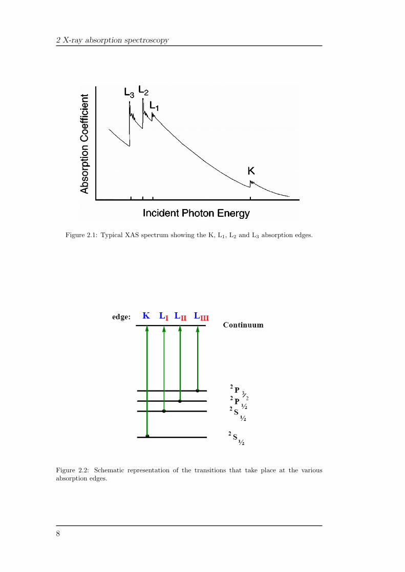
X-ray absorption spectroscopy (XAS) measures the X-ray absorption co-efficient, µ(E), as a function of the X-ray energy of the incident photon,E = ~ω (measured in eV). A XAS spectrum, in which the absorption coef-ficient is plotted as a function of E, shows an overall decrease of the X-rayabsorption with increasing energy, with the exception of very sharp peaks atcertain energies (called edges) due to the transitions of core electrons to highenergy states (see Figure 2.1). The energies of these peaks correspond to theionization energies of the core electrons. Each absorption edge is related toa specific atom present in the material and, more specifically, to a quantum-mechanical transition that excites a particular atomic core electron to thefree or unoccupied continuum levels. The nomenclature for X-ray absorptionreflects the origin of the core electron (see Figure 2.2). K edge refers to thetransition that excites the innermost 1s electron, L1 edge is due to the exci-tation of the 2s electron, while L2 and L3 edges are related to the excitationsof the 2p electrons with electronic states 2P1/2 and 2P3/2, respectively. Thetransitions are always to unoccupied states with the photoelectron above theFermi energy, which leaves behind a core hole. The energies of the edges areunique to the type of atom that absorbs in the X-ray and thus themselves aresignatures of the atomic species present in a material.
From what has been said, it is clear that XAS, being an atomic probe,places few constraints on the samples that can be studied. All atoms havecore level electrons, and XAS spectra can be measured for essentially everyelement on the periodic table. Moreover, crystallinity is not required for XASmeasurements (even if it is also possible to measure XAS spectra of crystallinesamples), making it one of the few structural probes available for noncrys-talline and highly disordered materials, including solutions, amorphous solidsand fluid samples in general. In many cases, XAS measurements can be madeon elements of minority and even trace abundance, giving a unique and directmeasurement of chemical and physical state of dilute species in a variety ofsystems. XAS spectra are recorded using the properties of synchrotron radi-ation, which provides tunable X-ray beams with high brilliance. In this way
7
2 X-ray absorption spectroscopy
Figure 2.1: Typical XAS spectrum showing the K, L1, L2 and L3 absorption edges.
Figure 2.2: Schematic representation of the transitions that take place at the variousabsorption edges.
8

2.1 Introduction
it is possible to obtain spectra with a very high signal/noise ratio.A typical XAS spectrum is shown in Figure 2.1. When the energy of the
incident photon, E, is greater than the ionization potential, E0, of a givenelectron, this electron is emitted by the photoabsorber atom with a kineticenergy equal to the difference E − E0 and undergoes a scattering process onthe nearest atoms. This phenomenon produces a series of wiggles or oscil-latory structures above the edge that modulate the absorption, typically bya few percent of the overall absorption cross section. These features containdetailed structural information on the atoms around the photoabsorber, suchas interatomic distances and coordination numbers. However, it is impor-tant to stress that the information on bond angles and distances that canbe obtained from a XAS spectrum is limited in a range of 4-5 A from thephotoabsorber atom [42]. The short-range character of XAS is due to thelimited mean free path of the photoelectron and to the excited state lifetime(core hole lifetime). In fact the high-energy excited photoelectron state is notlong lived, but must decay as a function of time and distance and thus cannotprobe long-range effects. This decay is due primarily to inelastic losses (i.e.“extrinsic losses”) as the photoelectron traverses the sample, either by inter-acting with and exciting other electrons, or by creating collective excitations(plasmon production). In addition, the intrinsic lifetime of the core-hole state(“intrinsic losses”) has to be clearly considered [42]. The net effect is thatXAS can only measure the local atomic structure over a range limited by thenet lifetime of the excited photoelectron. In this sense, XAS is very differ-ent from other techniques such as X-ray diffraction or neutron diffraction, inwhich also long-range interactions provide a detectable contribution to theexperimental spectrum.
A XAS spectrum is conventionally divided into two regions: the X-rayAbsorption Near Edge Structure (XANES) up to about 50 eV beyond the ab-sorption edge, and the Extended X-ray Absorption Fine Structure (EXAFS)at higher energies. The border between XANES and EXAFS regions is shownin Figure 2.3. The division of a XAS spectrum is only formal and it is dueto the different theoretical treatment and approximations used to calculatethe absorption cross section in the two regions. In both cases, a full quantumdescription of the X-ray absorption phenomenon is not possible, and, as aconsequence, approximate models have to be employed. In these models theemitted electron is treated as a quasi-particle (photoelectron) that moves inan effective potential which takes into account both the interaction with theother electrons of the photoabsorber atom and the potential generated by thesurrounding atoms. However, as the energy of the photoelectron increases,further approximations can be made to obtain a simpler data analysis proto-col. For this reason, historically the first quantitative analyses were made onthe high energy part of the absorption spectrum (EXAFS) while the XANESspectra have been analyzed for many years only on a qualitative way.
XAS phenomenon was discovered around 1930 but only 40 years later be-came a structural investigation technique, following the incoming of betterX-ray sources in the experiments and the development of theories able to
9

2 X-ray absorption spectroscopy
Figure 2.3: Division of the absorption spectrum between XANES and EXAFS regions.
provide a quantitative interpretation of experimental data. The first workswere published by Sayers et al. in 1971 and 1975 [43, 44]; in these works asemi-empiric parameterization of the EXAFS signal is proposed for the firsttime. Later, the work of different groups lead to the development of theoriesable to explain the many physical phenomena involved in radiation absorp-tion, confirming the validity of Sayers’ approach.
Some years ago a unifying scheme of interpretation of the X-ray absorp-tion spectra, based on the Multiple Scattering (MS) theory and valid forthe whole energy range, has been developed [45]. An important result ofthis MS approach, which is based on the Green’s function formalism, is thatthe expression for the absorption cross section (σ(E)) can be factored in anatomic term (σl
0(E)) depending only on atomic electronic properties, and ina structure factor (χl(E)) containing all the structural information on theenvironment:
σ(E) ∝ σl0(E)χl(E) (2.1)
The expression for χl(E) obtained within the MS theory is given by [46]:
χl(E) =1
(2l + 1)sin2δ0l
∑m
Im[(I + TaG)−1Ta]00lm,lm (2.2)
where I is the unit matrix, G is the matrix describing the spherical wavepropagation of the photoelectron from one site to another around the pho-toabsorber, T is the diagonal matrix describing the scattering process of thephotoelectron by the atoms located at the various sites around the photoab-sorber and δ0
l is the phase shift of the photoabsorbing atom (located at site
10
2.2 EXAFS analysis
0) for angular momentum l. Therefore, the fundamental problem in XAScalculations is the inversion of the matrix reported in equation 2.2. In thehigh energy region, this problem can be overcome by expanding the matrixinverse in a series in which each term corresponds to the contribution of ascattering path, or in other words, the matrix inverse can be written as a sumover all of the multiple scattering paths [46]. This is possible because in thehigh energy regime the series is convergent. Conversely, in the XANES regionthe series does not converge, and the structure factor has to be calculated bythe exact matrix inversion. This is one of the most fundamental differencesbetween the theoretical approaches used in the EXAFS and XANES regionsof the spectrum. The physical reason of this difference is that in the XANESregime the electron kinetic energy is small and the scattering on the neigh-bouring atoms tends to be strong, while the effect of the scatterers becomessmaller at higher energies and the photoelectron is only weakly scattered.
In this framework, several data analysis programs have been developedto analyze the experimental data. In these codes two fundamental approx-imations are generally used. The first one is the so called muffin-tin ap-proximation, in which the potential generated by the atoms surrounding thephotoabsorber is spherically averaged inside muffin-tin spheres around eachatom, and averaged to a constant in the interstitial region (delimited by aconvenient outer sphere enclosing the cluster used in the calculations). Thesecond approximation concerns the choice of the effective optical potential inwhich the photoelectron moves. The most used approximation is the complexHedin-Lundqvist energy dependent potential whose imaginary part accountsfor extrinsic losses [47]. While this approach is a good approximation inthe EXAFS region, in the low-energy regime the complex part of the Hedin-Lundqvist potential introduces an excessive loss in the transition amplitudeof the primary channel and thus other approximations are exploited, as weshall see in section 2.3.
In the remainder of this chapter a brief introduction to the techniquesused in the EXAFS and XANES data analysis will be given, with particularemphasis on their application to the study of disordered systems.
2.2 EXAFS analysis
The fundamental quantities used in the analysis of EXAFS spectra aredefined as follows:
• µ(E) is the atomic absorption coefficient, defined as the attenuation ofthe X-ray beam per distance unit, which is proportional to the absorp-tion cross section.
• µ0(E) is the absorption coefficient of the isolated atom.
• k =p
}=
√2me
}2(E − E0) is the photoelectron wave number.
11

2 X-ray absorption spectroscopy
Figure 2.4: Relation between µ(E), µ0(E) and χ(E).
• χ(k) = µ−µ0
µ0is the normalized oscillating part of the spectrum, which
is obtained by eliminating the absorption of the isolated atom from thesignal and normalizing it to unity.
The relation between these quantities is shown in figure 2.4. χ(k) contains allthe structural information on the system in an analogous way to the structurefactor S(q) in diffraction techniques.
Sayers et al. developed a quantitative parameterization of χ(k) which hasbecome the standard for current EXAFS analysis and it is given by [43]:
χ(k) = S20
∑i
Nifi(k)
kR2i
sin(2kRi + 2δc(k) + φi(k))e−2Riλ(k) e−2σ2
i k2
(2.3)
where S20 is a phase reduction factor, the index i is related to the Ni equiva-
lent scattering atoms at distance Ri from the photoabsorber, δc(k) and φi(k)are the phase displacements due to the photoabsorber atom and to the scat-terers, respectively. σi is the average square fluctuation of the bond distances(or Debye-Waller factor) and contains the structural disorder, and fi is thediffusion amplitude. The substantial validity of this expression is due to theabove mentioned fact that in the high energy range the contributions of thedifferent scattering paths can be factorized and for the special case in whichonly two-body paths are accounted for, the functional form of equation 2.3 isrecovered.
The Debye-Waller factor in equation 2.3 accounts for the fact that, dueto the thermal vibrations, the atomic positions oscillate and thus Ri is onlythe average value of a distance distribution. For low enough temperatures,i.e. in the harmonic approximation limit, this distribution is well approx-
12

2.2 EXAFS analysis
imated by a Gaussian function of width proportional to the Debye-Wallerfactor (this is the origin of the e−2σik
2term in equation 2.3). The analysis
of crystalline samples is usually made describing the coordination around thephotoabsorber atom using these Gaussian shells. On the other hand, at ele-vated temperatures or in disordered systems, such as aqueous ionic solutions,the distribution functions become broad and asymmetric towards the largedistances, the harmonic approximation is no longer valid and the appropriatedescription of these systems can be performed in terms of radial distributionfunctions (g(r)). When an asymmetric distribution is present the first peak ofthe radial distribution functions can be modeled using a set of Gamma func-tions. These functions are described by an average distance R, a coordinationnumber (Nc), a standard deviation σ, and an asymmetry factor (skewness)
β = 2p12 . Their general expression is given by:
f(r) = Ncp
12
σΓ(p)
[p +
r − R
σp
12
](p−1)
e−
hp+ r−R
σp
12
i(2.4)
where Γ(p) is the Euler Gamma function associated to the parameter p.The EXAFS spectroscopy is particularly suited to the study of the lo-
cal environment around a photoabsorber atom, such as an ion in aqueoussolution, since the EXAFS signal depends only on the distribution functionsrelated to photoabsorber atom; this is one of its main advantages over diffrac-tion techniques where the structure factor S(q) is the superimposition of theN(N + 1)/2 different distribution functions associated to the N atoms of thesystems, and it is very difficult to isolate single contributions. Therefore, insystems like ionic solutions the greater contribution to the structure factor isfrom bulk water and diffraction techniques can be employed only in ratherconcentrated solutions (1-2 M), while EXAFS can be used at very low con-centrations. Moreover, EXAFS provides values of bond distances with veryhigh accuracy, typically of the order of 0.01 A, about one order of magni-tude greater than the majority of diffraction techniques. On the other hand,EXAFS can only give short range (up to 4-5 A) information, as it has beenalready discussed in the previous section, and, in the case of disordered sys-tems, the fitting parameters are often correlated and the EXAFS data anal-ysis can lead to ambiguous result. A strategy to help in the extraction of thestructural details contained in the EXAFS spectra of disordered systems is toinclude independent information derived from computer simulations. In par-ticular, in recent years it has been shown that EXAFS data analysis of ionsand molecules in solution can derive strong benefit by using the radial distri-bution functions calculated from Molecular Dynamics simulations as startingmodels. In this case the theoretical signal χ(k), associated for example to theion-oxygen distribution in an aqueous ionic solution, is expressed as a functionof the ion-oxygen g(r) calculated from the Molecular Dynamics trajectories:
χ(k) =
∫ ∞
0
dr4πr2ρg(r)A(k, r) sin(2kr + φ(k, r)) (2.5)
13

2 X-ray absorption spectroscopy
where A(k, r) and φ(k, r) are amplitude and phase functions and ρ is the den-sity of scattering atoms. With such a procedure, it is possible to analyze theEXAFS data using a realistic structural model and including the contributionof the second hydration shell.
The theoretical signal is then compared with the experimental one byminimizing the following function:
Ri({λ}) =N∑
i=1
[αexp(Ei) − αmod(Ei; λ1 . . . λp)]2
σ2i
(2.6)
where N is the number of experimental points Ei, {λi} is the set of p parame-ters that are optimized and σ2
i is the variance associated to each experimentaldatum αexp(Ei). On the basis of the final value of Ri({λ}) and of the agree-ment between the experimental and theoretical spectra, the correctness of thestarting g(r) can be evaluated. Therefore, this combined EXAFS-MolecularDynamics approach on the one hand allows one to verify the reliability of theMolecular Dynamics simulations by comparing the theoretical results withthe experimental data, on the other hand provides a useful starting model inthe EXAFS analysis of disordered systems. The structural parameters of thestarting model can be fitted in order to obtain the better possible agreementwith the experimental data, and an accurate description of the first coordi-nation shell can thus be obtained.
It is important to stress that besides the radial (two-body) distributionfunctions, also information on three-body, four-body . . . distribution functionscan be obtained from the EXAFS analysis, that are calculated by means of theMS theory as implemented in the GNXAS software package [48]. Obviously,this is possible only when MS processes provide a detectable contribution tothe EXAFS experimental spectrum.
2.3 XANES analysis
The XANES region of the spectrum is extremely sensitive to the geomet-ric environment of the absorbing atom and, in principle, an almost completerecovery of the three-dimensional structure can be achieved from it. The pos-sibility to gain structural information from the XANES spectra is extremelyimportant for dilute and biological systems where the low signal-to-noise ratioof the experimental data hampers a reliable analysis of the EXAFS region.Moreover, in the study of disordered systems coordination numbers cannotbe accurately determined from the EXAFS data due to their large correla-tion with the Debye-Waller factors, and for these systems the analysis of theXANES region can thus be essential to address some of the shortcomings ofEXAFS. However, the analysis of the low-energy part is much more difficultto be performed due to the theoretical approximation in the treatment ofthe potential [49] and requires the use of heavy time-consuming algorithms[50] to calculate the absorption cross section in the framework of the full MSapproach. For this reason, this technique has been for a long time used as a
14

2.3 XANES analysis
qualitative method used as a help for standard EXAFS studies [51] and onlysome years ago some methods have been proposed in the literature whichperforms a quantitative analysis of XANES [52]. In particular a new softwareprocedure, named MXAN, has been developed [34]. This method is basedon the comparison between the XANES experimental spectrum and severaltheoretical calculations performed by varying selected structural parametersassociated with a given starting model. Starting from a putative geometricalconfiguration around the photoabsorber atom, the MXAN package is able toreach the best-fit conditions in a reasonable time, by minimizing a residualfunction Rsq in the space of the structural and non-structural parametersdefined as:
Rsq = n
∑mi=1 wi
[(yth
i − yexpi )ε−1
i
]2∑mi=1 wi
(2.7)
where n is the number of independent parameters, m is the number of ex-perimental points, yth
i and yexpi are the theoretical and experimental values
of the cross section, εi is the error on each experimental point and wi thestatistical weights. The X-ray absorption cross section is calculated usingthe full MS scheme within the muffin-tin approximation for the shape of thepotential. The exchange and correlation part of the potential are determinedon the basis of the local density approximation of the self-energy of the pho-toelectron using an appropriate complex optical potential. The real part ofthe self-energy is calculated either by the Hedin-Lundqvist energy-dependentpotential or by the Xα approximation. However, to avoid over-damping atlow energies due to the complex part of the Hedin-Lundqvist potential, theMXAN method can account for all inelastic processes by convolution with abroadening Lorentzian function having an energy-dependent width Γtot(E) ofthe form [34]:
Γtot(E) = Γc + Γmfp(E) (2.8)
The constant part Γc accounts for both the experimental resolution and thecore-hole lifetime, while the energy dependent term Γmfp(E) represents allthe intrinsic and extrinsic inelastic processes. The Γmfp(E) is zero below anenergy onset Es (which, in extended systems, correspond to the plasmon ex-citation energy), and starts increasing from a given value A, following theuniversal form of the mean free path in solids [53].
The MXAN procedure has been successfully applied to the study of severalsystems, both in the solid and liquid state, allowing a quantitative extractionof the relevant geometrical information about the absorbing site [54, 35, 56].However, in the case of ionic solutions the XANES spectra have been usuallycomputed reducing the system to a single structure since the contributionfrom molecules and arrangements instantaneously distorted cannot be calcu-lated using the analysis standard methods. A promising strategy to overcomethis problem is to analyze the XANES spectra using the microscopic dynam-ical description of the system derived from Molecular Dynamics simulations.In this framework, we have developed a computational procedure which usesMXAN and Molecular Dynamics simulations to generate a configurational av-
15

2 X-ray absorption spectroscopy
eraged XANES spectrum and we have applied it to the study of ionic aqueoussolutions.
16

Chapter 3
Molecular DynamicsSimulations
Molecular Dynamics, strictly speaking, is the simultaneous motion ofatomic nuclei and electrons forming molecular entities. A complete descrip-tion of such a system requires in principle solving the full time-dependentSchrodinger equation including both electronic and nuclear degrees of free-dom. This is however a too much expensive computational task which is inpractice unfeasible for systems consisting of more than three atoms. In or-der to study the dynamics of the vast majority of chemical systems severalapproximations have therefore to be introduced. First of all, it is assumed inMolecular Dynamics with the Born-Oppenheimer approximation that the mo-tion of electrons and nuclei is separable, and the electron cloud adjusts instan-taneously to changes in the nuclear configuration. As a consequence, nuclearmotion evolves on a PES, associated with the electronic quantum state whichis obtained by solving the time-independent electronic Schrodinger equationfor a series of fixed nuclear geometries. In practice, most Molecular Dynamicssimulations are performed on the ground state PES.
Moreover, in addition to making the Born-Oppenheimer approximation,Molecular Dynamics treats the atomic nuclei as classical particles whose tra-jectories are computed using the laws of classical mechanics. This is a verygood approximation for molecular systems as long as the properties studiedare not related to the motion of light atoms (like the hydrogen atoms, whichshow quantum mechanical behaviour in certain situations such as tunnelingphenomena) or vibrations with frequency ν such that hν > kBT .
The potential functions which describe the intermolecular and intramolec-ular interactions between classical nuclei can be treated at various levels ofapproximation. In classical Molecular Dynamics the interaction potential isexpressed as a simple sum of pair potentials. On the other hand, ab ini-tio Molecular Dynamics computes interactions at a much more fundamentallevel using electronic structure methods. In the mixed Quantum Mechani-cal and Molecular Mechanics (QM/MM) methods instead the “important”part of the system, for instance where a chemical reaction is taking place, istreated with electronic structure calculations whereas the rest of the system
17

3 Molecular Dynamics Simulations
is described by a classical force field. In this chapter an introduction to theclassical Molecular Dynamics is given, followed by a brief description of thepolarization in molecular simulation.
3.1 Classical Molecular Dynamics
In the classical Molecular Dynamics simulations the time evolution of asystem composed by M particles (generally atoms) is obtained by solving theNewton’s equation of motion step-by-step [59]:
MaRa = Fa a = 1, 2, . . . ,M (3.1)
where Ma and Ra are the mass and the position of particle a and Fa is theforce acting on particle a given by:
Fa = − ∂V
∂Ra
(3.2)
V is a potential energy function which depends on the complete set of 3Mparticle coordinates. In classical Molecular Dynamics the complex potentialenergy function is represented by a sum of simple functions, called force fields.In these force fields, the interactions are usually divided into bonded and non-bonded [60]:
V = Vbonded + Vnon−bonded (3.3)
Bonded interactions are written as a sum of various terms:
Vbonded = Vbonds + Vangles + Vdihedrals + Vimpr−dihedr (3.4)
Vbonds describes the stretching between the atoms in the system covalentlybonded:
Vbonds =∑bonds
1
2kbij
(bij − b0ij)
2 (3.5)
where the covalent bond between atoms i and j is represented by a harmonicpotential with force constant kbij, instantaneous distance bij and equilibriumdistance b0
ij. For some systems that require an anharmonic bond stretchingpotential, other functional forms can be used such as the Morse potential [61].Vangles describes the bond angle vibrations:
Vangles =∑
angles
1
2kθijk
(θijk − θ0ijk)
2 (3.6)
where the bending of the bond angle between a triplets of atoms i, j and k ismodeled by a harmonic potential with force constant kθijk
, instantaneous an-gle θijk and equilibrium angle θ0
ijk. Vdihedrals mimics the vibrations of dihedral
18
3.1 Classical Molecular Dynamics
angle (four-body) interactions and is generally modeled as:
Vdihedrals =∑
dihedrals
1
2kφijkl
[1 + cos(nφijkl − γ)] (3.7)
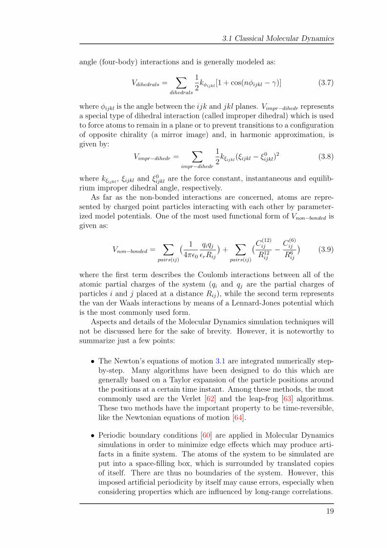
where φijkl is the angle between the ijk and jkl planes. Vimpr−dihedr representsa special type of dihedral interaction (called improper dihedral) which is usedto force atoms to remain in a plane or to prevent transitions to a configurationof opposite chirality (a mirror image) and, in harmonic approximation, isgiven by:
Vimpr−dihedr =∑
impr−dihedr
1
2kξijkl
(ξijkl − ξ0ijkl)
2 (3.8)
where kξijkl, ξijkl and ξ0
ijkl are the force constant, instantaneous and equilib-rium improper dihedral angle, respectively.
As far as the non-bonded interactions are concerned, atoms are repre-sented by charged point particles interacting with each other by parameter-ized model potentials. One of the most used functional form of Vnon−bonded isgiven as:
Vnon−bonded =∑
pairs(ij)
( 1
4πε0
qiqj
εrRij
)+
∑pairs(ij)
(C(12)ij
R12ij
−C
(6)ij
R6ij
)(3.9)
where the first term describes the Coulomb interactions between all of theatomic partial charges of the system (qi and qj are the partial charges ofparticles i and j placed at a distance Rij), while the second term representsthe van der Waals interactions by means of a Lennard-Jones potential whichis the most commonly used form.
Aspects and details of the Molecular Dynamics simulation techniques willnot be discussed here for the sake of brevity. However, it is noteworthy tosummarize just a few points:
• The Newton’s equations of motion 3.1 are integrated numerically step-by-step. Many algorithms have been designed to do this which aregenerally based on a Taylor expansion of the particle positions aroundthe positions at a certain time instant. Among these methods, the mostcommonly used are the Verlet [62] and the leap-frog [63] algorithms.These two methods have the important property to be time-reversible,like the Newtonian equations of motion [64].
• Periodic boundary conditions [60] are applied in Molecular Dynamicssimulations in order to minimize edge effects which may produce arti-facts in a finite system. The atoms of the system to be simulated areput into a space-filling box, which is surrounded by translated copiesof itself. There are thus no boundaries of the system. However, thisimposed artificial periodicity by itself may cause errors, especially whenconsidering properties which are influenced by long-range correlations.
19
3 Molecular Dynamics Simulations
• Long range non-bonded interactions are generally not calculated beyonda certain cutoff distance around each particle, in order to reduce thecomputational cost of the simulations. However, as far as the Coulombinteractions are concerned, the use of a simple cutoff can introduceserious artifacts and, for this reason, several techniques have been de-veloped for handling long range interactions, the most popular of thembeing the Ewald summation [65] and the Particle Mesh Ewald methods[66, 67].
• Constraints are often used in Molecular Dynamics simulations, i.e. bondsare treated as being constrained to have fixed length. This is very usefulwhen bonds have very high vibration frequencies and should be treatedin a quantum mechanical way rather than in the classical approxima-tion. Moreover, they allow to increase the integration time step andthus to perform longer simulations. The most commonly used con-straints methods are the LINCS [68] and SHAKE [69] algorithms.
• When solving the Newton’s equations of motion 3.1 the energy is a con-stant of motion and the simulation is performed in an NVE ensemble.However, it is often more convenient to carry out simulations in otherensembles, such as NVT or NPT. To this end, several approaches havebeen developed which control the temperature and the pressure of asystem. As far as the temperature control is concerned, widely usedtechniques are the Berendsen [70] and Nose-Hoover [71, 72] methods,while for the pressure control the Parrinello-Rahman scheme [73, 74] isextensively employed.
3.2 Accounting for polarization in molecular
simulation
Polarization plays an important role in the energetics of molecular sys-tems. Most computer simulation studies do not treat electronic polarizabilityexplicitly, but only implicitly using effective charges, dielectric permittivitiesor continuum electrostatics methods. Yet, the introduction of explicit po-larizability into molecular models and force fields is unavoidable when moreaccurate simulation results are to be obtained. If the polarization is not takeninto account, the electrostatic energy Velec corresponds to a pure Coulomb in-teraction:
Velec =1
2
∑pairs(ij)
(qiqj
rij
)(3.10)
Various ways to account for polarizability in molecular simulation exist andone strategy consists in assigning isotropic polarizabilities and induced dipolesat each atomic site.In this framework the energy Velec is composed of a charge-
20

3.2 Accounting for polarization in molecular simulation
charge interaction, charge-dipole and dipole-dipole energy:
Velec =1
2
∑pairs(ij)
[qiqj
rij
+1
r3ij
(−qipj + qjpi) ·rij +pi ·Tij ·pj
]+
1
2
∑i
pi ·αi−1 ·pi
(3.11)where, following Thole’s induced dipole model [57] each atomic site i car-
ries one permanent charge qi and one induced dipole pi associated with anisotropic atomic polarizability tensor αi, rij=ri - rj:
Tij =1
r3ij
(1 − 3
riirij
r2ij
)(3.12)
and1
2
∑i
pi · αi−1 · pi (3.13)
is the polarization energy.
21

3 Molecular Dynamics Simulations
22

Chapter 4
Methods employed in the studyof lanthanoids aqua ions
4.1 X-ray absorption spectroscopy
4.1.1 X-ray absorption measurements
Aqueous solutions of the lanthanoid(III) ions (Ln(III)) were made bydissolving a weighed amount of hydrated trifluoromethanesulfonates salts[Ln(H2O)n](CF3SO3)3 (in which Ln=Nd, Gd, Yb and Lu) in freshly dis-tilled water. The concentration of the samples was 0.2 M and the solu-tions were acidified to about pH=1 by adding trifluoromethanesulforic acidto avoid hydrolysis. Solid [Nd(H2O)9](CF3SO3)3, [Gd(H2O)9](CF3SO3)3,[Yb(H2O)8.7](CF3SO3)3 and [Lu(H2O)8.2](CF3SO3)3 were diluted with boronnitride to give an absorption change over the edge of about one logarithmicunit. The K-edge spectra were collected at ESRF, on the bending magnetX-ray absorption spectroscopy beamline BM29 [75] in transmission geometry.The storage ring was operating in 16-bunch mode with a typical current of80 mA after refill. The aqueous solutions were kept in cells with Kapton filmwindows and Teflon spacers ranging from 2 to 3 cm depending on the sample.The L3-edge measurements were performed at the wiggler beamline 4-1 atthe Stanford Synchrotron Radiation Laboratory (SSRL), Stanford, U.S.A.,which was operated at 3.0 GeV and a maximum current of 100 mA. In thiscase simultaneous data collection was performed both in transmission andfluorescence mode. The stations at ESRF and SSRL were equipped with aSi[511] and Si[111] double-crystal monochromator, respectively. Higher orderharmonics were reduced by detuning the second monochromator crystal toreflect, at the end of the scans, 80% of maximum intensity at the K-edgeenergies and 30-50% of maximum intensity at the L3-edges, with the lowervalue at lower energy. Internal energy calibration was made when possiblewith a foil of the corresponding lanthanoid metal.
23

4 Methods employed in the study of lanthanoids aqua ions
4.1.2 XANES data analysis
The quantitative XANES data analysis of the crystalline samples and theaqueous solution with a static model has been performed by means of theMXAN procedure which is described in section 2.3.
The K-edge XANES spectra of lanthanoid(III) ions are strongly affectedby the short core-hole lifetime of the excited photoelectron (the core-holewidths at the K-edges are Γ=17.3, 22.3, 31.9 and 33.7 eV for Nd, Gd, Yband Lu respectively [76]). As a consequence the edge resonance is stronglydamped and the intensity of the main transition peaks becomes very small.Recently, core-hole width deconvolution methods have been developed [77]and applied to the analysis of the XANES spectra at the Hg L3 and Cd K-edges [78, 36, 79]. This treatment largely facilitates the detection of spectralfeatures and the comparison with theoretical calculations. Even if in prin-ciple the deconvolution procedure could introduce small distortions in theexperimental data, the advantage of this approach is to avoid the use of thephenomenological broadening function in the calculation of the theoreticalspectrum to mimic electronic damping. In the present case the Nd, Gd, Yband Lu K-edge raw experimental data have been deconvolved of the whole tab-ulated core hole width and a Gaussian filter with full width at half-maximumof about 7.4, 8.0, 12.4 and 14 eV has been used, for Nd, Gd, Yb, and Lu re-spectively. The MXAN fitting procedure has been applied to lanthanoid(III)ions in hydrated trifluoromethanesulfonate crystals including either the firstshell water molecules only or the first plus the second coordination shells. Thehydrogen atoms were always included in the analyses. The cluster size andthe lmax value (i.e., the maximum l-value of the spherical harmonic expansionof the scattering path operators) were chosen on the basis of a convergencecriterion.
The XANES spectra of Ln(III) ions in aqueous solution have been ana-lyzed starting from the microscopic description of the system derived fromMD simulations. In the first step the XANES spectra associated with theMD trajectories have been calculated using only the real part of the HL po-tential. In this way the theoretical spectra do not account for any intrinsicand extrinsic inelastic process. In the second step a minimization in the non-structural parameter space has been carried out to perform a comparison withthe experimental data. In particular, the inelastic processes are accounted forby convolution with the broadening Lorentzian function defined by equation2.8. In the case of the K-edge XANES deconvolved spectra the constant partΓc, which accounts for the core-hole lifetime, has not been included in ourcalculations as it has been removed from the experimental data. For the L3-edge spectra fixed Γc values of 4.60, 3.65, and 4.01 eV have been used for Yb,Nd, and Gd, respectively. In all cases the experimental resolution has beentaken into account by convolution with a Gaussian function whose widthsΓexp are reported in Table 6.2. For each ion two MD trajectories havebeen extracted from the total simulation, the former containing the first shellnonahydrated cluster only, the latter containing both the first and the secondhydration shells. In particular, we have considered all the water molecules
24
4.1 X-ray absorption spectroscopy
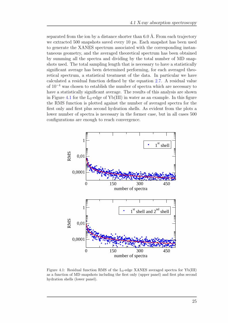
separated from the ion by a distance shorter than 6.0 A. From each trajectorywe extracted 500 snapshots saved every 10 ps. Each snapshot has been usedto generate the XANES spectrum associated with the corresponding instan-taneous geometry, and the averaged theoretical spectrum has been obtainedby summing all the spectra and dividing by the total number of MD snap-shots used. The total sampling length that is necessary to have a statisticallysignificant average has been determined performing, for each averaged theo-retical spectrum, a statistical treatment of the data. In particular we havecalculated a residual function defined by the equation 2.7. A residual valueof 10−4 was chosen to establish the number of spectra which are necessary tohave a statistically significant average. The results of this analysis are shownin Figure 4.1 for the L3-edge of Yb(III) in water as an example. In this figurethe RMS function is plotted against the number of averaged spectra for thefirst only and first plus second hydration shells. As evident from the plots alower number of spectra is necessary in the former case, but in all cases 500configurations are enough to reach convergence.
0 150 300 450number of spectra
0,0001
0,01
1
RM
S
1st shell
0 150 300 450number of spectra
0,0001
0,01
1
RM
S
1st shell and 2
nd shell
Figure 4.1: Residual function RMS of the L3-edge XANES averaged spectra for Yb(III)as a function of MD snapshots including the first only (upper panel) and first plus secondhydration shells (lower panel).
25

4 Methods employed in the study of lanthanoids aqua ions
4.1.3 EXAFS data analysis
In the standard EXAFS analysis of disordered systems only two-bodydistributions are usually included, and the χ(k) signal is represented by theequation 2.5. As already mentioned in section 2.2, χ(k) theoretical signalscan be calculated by introducing in equation 2.5 the model radial distributionfunctions obtained from Molecular Dynamics simulations. In all the aqueoussolutions studied, both the M-O and M-H g(r)’s obtained from the simulationshave been used to calculate the single scattering first shell χ(k) theoreticalsignal, as the ion-hydrogen interactions have been found to provide a de-tectable contribution to the EXAFS spectra of several metal ions in aqueoussolutions [80, 81]. Comparison of the total theoretical and experimental χ(k)signals allows the reliability of the g(r)’s, and consequently of the theoreti-cal scheme used in the simulations, to be checked. In this case, i.e. whena direct comparison between the signal obtained from Molecular Dynamicssimulations and the experimental one is performed, the structural parametersare kept fixed during the minimization, while two nonstructural parametersare optimized: S2
0 , which is a many-body amplitude reduction factor due tointrinsic losses, and E0, which aligns the experimental and theoretical energyscales. On the other hand, the theoretical χ(k) signal can also be refinedagainst the experimental data in order to obtain the better possible agree-ment between the two spectra. In this latter case, the fitting is performedby using a least-squares minimization procedure in which structural and non-structural parameters are allowed to float [82]. Since a correct description ofthe first coordination sphere of hydrated metal complexes has to account forthe asymmetry in the distribution of the ion-solvent distances, the M-O andM-H g(r)’s associated with the first coordination shells were modeled withΓ-like distribution functions which depend on four parameters, namely thecoordination number Nc, the average distance R, a standard deviation σ, andthe skewness (see section 2.2).
The EXAFS theoretical signals have been calculated by means of theGNXAS code which uses an advanced theoretical scheme based on the multiple-scattering formalism [48]. Phase shifts, A(k,r) and φ(k,r), have been calcu-lated starting from a configuration extracted from the Molecular Dynam-ics simulation, by using muffin-tin potentials and advanced models for theexchange-correlation self-energy (Hedin-Lundqvist) [47]. Inelastic losses ofthe photoelectron in the final state have been accounted for intrinsically bycomplex potential. The imaginary part also includes a constant factor ac-counting for the core-hole width.
4.2 MD simulations
MD simulations of Nd(III), Gd(III), and Yb(III) ions in aqueous solu-tion have been performed using the ab initio effective two-body potentialsdeveloped by Floris et al. [5], obtained by fitting the parameters of a suit-able analytical function on an ab initio potential energy surface. The SPC/E
26

4.3 Polarised MD simulations
water intramolecular potential was used in the fitting procedure [83]. Threeuncharged massless interaction sites were added to the water molecule: two ofthese (L1 and L2) are symmetrically located on the axis going through the Oatom, perpendicular to the water molecular plane; the third virtual site (L3)is on the C2 axis on the opposite side with respect to the hydrogen atoms. Athorough description of the procedure used to obtain the ab initio potentialenergy function can be found in ref [5]. The potential functions have thefollowing analytical form:
UMi(r) = UCoul + Air−4Mi + Bir
−6Mi + Cir
−8Mi + Dir
−12Mi + Fie
−GirMi (4.1)
where UCoul is the Coulomb interaction computed with atomic charges as inthe SPC/E model [83], M stands for one of three lanthanoid ions and i is aninteraction site on water, that is, the water oxygen and hydrogen atoms andthe three dummy atoms and rMi is the ion-interaction site distance. Ai,..., Gi
are the potential function parameters obtained by the fitting procedure (seeTable 2 of ref [5]). The simulated systems were composed by one Ln(III) ionand 809 water molecules (for a total of 4855 atoms and virtual interactionsites) in a cubic box, using periodic boundary conditions. The box side wasalways 29.054 A. All simulations were performed in a NVT ensemble at 300 Kusing the Berendsen method [84] with a coupling constant of 0.01 ps. A timestep of 1 fs was used, saving a configuration every 25 time steps. Calculationswere carried out using the GROMACS package version 3.2.1 [85] modifiedto include the effective pair potentials. Short-range interactions have beentruncated at 9 A and the Particle Mesh Ewald [66, 67] method was employedto treat long-range electrostatic effects while an homogeneous backgroundcharge has been used to compensate for the presence of the Ln(III) ion [86].MD simulations of 5 ns were used to sample each of the three systems, afteran equilibration phase of 1 ns.
4.3 Polarised MD simulations
MD simulations of lanthanoids ions in aqueous solution, taking into ac-count the polarization, have been performed using the procedure developedby M. Duvail et al. described in references [58]. The total potential energyof the system is modeled as a sum of different terms:
Vtot = Velec + V LJO−O + VLn−O (4.2)
where Velec is the electrostatic energy term defined by equation 3.10 and VO−O
is the 12-6 Lennard-Jones potential describing the O-O interaction. Becauseof the explicit polarization introduced in the model, the original TIP3P water[87] was modified into the TIP3P/P water model [16], i.e., the charges on Oand H were rescaled to reproduce correctly the dipole moment of liquid water.VLn−O account for the nonelectrostatic Ln-O interaction potential. The po-tential is composed by a long range attractive part with a 1/r6 behavior and a
27

4 Methods employed in the study of lanthanoids aqua ions
short range repulsive part modeled via an exponential function, dealing withthe well-known Buckingham exponential-6 potential (Buck6):
V Buck6ij = Aijexp(−Bijrij) −
Cij
r6ij
(4.3)
The Ln-O Buck6 parameters are estimated from extrapolating the originalLa-O Buck6 parameters obtained by fitting the Møller-Plesset perturbation(MP2) potential energy curve [16], while for all the other lanthanoid ions theBuck6 parameters were extrapolated using the Shannon ionic radii [88].Simulations of the hydrated Ln(III) ions have been carried out in the micro-canonical NVE ensemble with a own developed classical molecular dynamicsCLMD code MDVRY [89] using a Car-Parrinello-like scheme to obtain atomicinduced dipoles [90].CCLMD simulations were performed for one Ln(III) and 216 rigid watermolecules in a cubic box at room temperature. As previously reported [16]test simulations with a 1000 water molecules box provide the same results andthus was used this relatively small box to simulate many systems with alsodifferent sets of parameters for each system. Simulations were done on a 2.4GHz AMD Opteron CPU and each simulation takes about 10 h/ns. Periodicboundary conditions were applied to the simulation box. Long-range interac-tions have been calculated by using smooth particle mesh Ewald method [67].Simulations were performed using a velocity-Verlet-based multiple time scalefor the simulations with the TIP3P/P water model. Equations of motion werenumerically integrated using a 1 fs time step. The system was equilibratedat 298 K for 2 ps. Production runs were subsequently collected for 3 ns. Theaverage temperature was 293 K with a standard deviation of 10 K.
28

Chapter 5
Structures of solvated Nd(III),Gd(III), Yb(III) and Lu(III) inaqueous solution and crystallinesalts
5.1 Hydrated lutetium(III) ions in aqueous
solution and in the trifluoromethanesul-
fonate salt
To shed light on the geometry of the hydration complex of the Ln(III) ionsin aqueous solution, a useful strategy is to use solid salts of known structureas starting coordination models. To this end we have collected the XANESspectra at the K- and L3-edge of [Lu(H2O)8.2](CF3SO3)3 . This compoundhas been chosen because the water molecules in the first coordination shellare arranged in a distorted TTP geometry. In the low-temperature structure,the six Lu-O bond lengths in the fairly regular trigonal prism are in the range2.272(4)-2.296(4) A, one capping site is fully occupied with a Lu-O length of2.395(4) A, whereas for the two more distant capping sites the Lu-O distancesare 2.555(6) and 2.568(6) A with occupancy factors of 0.58(1) and 0.59(1),respectively [15]. The high-temperature phase can be regarded as an averageof the low-temperature structure as previously discussed [15]. This is furthersupported by the fact that the structure of the high-temperature phase as de-termined by EXAFS, which is lattice independent, is in full agreement withthe low-temperature phase. This shows that the geometry of the hydratedlutetium(III) ion observed in the low-temperature phase is also present atroom temperature and in aqueous solution [15]. The raw K-edge spectrum ofsolid [Lu(H2O)8.2](CF3SO3)3 is compared with the spectrum of lutetium(III)in aqueous solution in the upper panel of Figure 5.1. The two spectra areidentical in the whole energy range suggesting that the coordination of thelutetium(III) ion in the two systems is the same. However, owing to the shortlifetime of the excited atomic state, both the edge resonance and the struc-
29

5 Structures of solvated Nd(III), Gd(III), Yb(III) and Lu(III) in aqueoussolution and crystalline salts
0 50 100 150
0.6
0.8
1
Nor
mal
ized
abs
orpt
ion
(arb
. uni
ts)
SolidSolution
0 50 100 150
E − E0 (eV)
0.5
1
SolidSolution
Figure 5.1: Upper panel: Comparison between the raw K-edge XANES spectra oflutetium(III) in aqueous solution (solid line) and solid [Lu(H2O)8.2](CF3SO3)3 (red dot-ted line). Lower panel: Comparison between the K-edge deconvolved XANES spectra oflutetium(III) in aqueous solution (solid line) and solid [Lu(H2O)8.2](CF3SO3)3 (dotted redline).
tural oscillations are strongly damped. Therefore, we have applied a core-holewidth deconvolution procedure [77] to the XANES spectra of both the solidand aqueous solution samples. The whole tabulated core-hole width (Γ=33.7eV) [76] has been removed from the K-edge raw experimental data, and aGaussian filter with full width at half maximum of about 14 eV has been ap-plied. After deconvolution, the threshold regions are considerably sharpenedwith respect to the original spectra, and the intensity of the structural oscilla-tions is also clearly enhanced (see lower panel of Figure 5.1). Also, in this casethe XANES spectrum of lutetium(III) in aqueous solution is identical to thesolid lutetium(III) trifluoromethanesulfonate one, reinforcing the similarityof the first-neighbor coordination geometry. In the first step of the analysis,the reliability of the MXAN method has been tested by applying a minimiza-tion procedure to both the raw and deconvolved K-edge XANES spectra of
30

5.1 Hydrated lutetium(III) ions in aqueous solution and in thetrifluoromethanesulfonate salt
solid lutetium(III) trifluoromethanesulfonate. The analysis has been carriedout starting from the low-temperature crystallographic structure [15], andby refining the structural and nonstructural parameters. In the fits, eightwater molecules were included: six in the prism sites at the same distanceand two in the capping sites with different Lu-O bond lengths. Note that thehydrogen atoms have been included in the analysis. The results of the fittingprocedures are shown in Figure 5.2 for the raw and deconvolved spectra, andthe bond metrics are detailed in Table 5.1.
0 50 100 150
0.6
0.8
1
Nor
mal
ized
abs
orpt
ion
(arb
. uni
ts)
0 50 100 150
E − E0 (eV)
0.5
1
Lu(III)
Figure 5.2: Upper panel: Comparison between the raw K-edge XANES experimental spec-trum of solid [Lu(H2O)8.2](CF3SO3)3 (dashed blue line) and the theoretical spectrum in-cluding the first coordination shell only (solid red line). Lower panel: Comparison betweenthe K-edge XANES deconvolved experimental spectrum of solid [Lu(H2O)8.2](CF3SO3)3(dashed blue line) and the theoretical spectrum including the first coordination shell only(solid red line).
The agreement between the experiment and the calculated model is quitegood in the case of the raw data [Rsq=2.3, in which Rsq is the square resid-ual function, see Eq. 2.7] and it improves for the deconvolution spectrum(Rsq= 1.2). It is known that systematic errors in the MXAN analysis can
31
5 Structures of solvated Nd(III), Gd(III), Yb(III) and Lu(III) in aqueoussolution and crystalline salts
arise mostly because of the poor approximation used for the phenomenologi-cal broadening function Γ(E) that mimics the electronic damping [55, 91, 92].This can explain the better agreement between the experimental and calcu-lated spectrum obtained for the deconvolved data. Note that the structuralparameters obtained from the two analyses are equal within the statisticalerrors, and are in good agreement with the crystallographic determination.However, as expected, the statistical errors obtained from the minimizationare slighter larger in the case of the raw data, as compared with the decon-volved data. As far as the non structural parameters are concerned, the Γvalues obtained from the raw and deconvolved data are 26 and 10 eV, respec-tively.
Fitting procedures have also been applied to the raw and deconvolvedXANES spectra of the aqueous solution of lutetium(III) by using the low-temperature crystallographic structure of [Lu(H2O)8.2](CF3SO3)3 as a start-ing model. The best-fit results are identical to those obtained for the tri-fluoromethanesulfonate crystal, both for the raw and deconvolved data (seeTable 5.1).
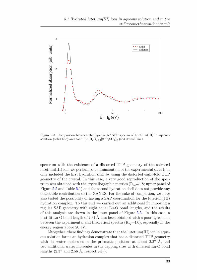
A different picture emerges from the comparison between the L3-edgeXANES spectra of lutetium(III) in aqueous solution and solid trifluorome-thanesulfonate (Figure 5.3). In this case, the two spectra show sizeable dif-ferences both in the edge and higher-energy region. In particular, both spec-tra have a sharp main peak followed by the structural oscillations, but thesolid sample shows two additional humps at about 18 and 48 eV that are notpresent in the aqueous solution spectrum. To unveil the origin of this differ-ence we have carried out a quantitative analysis of the L3-edge XANES dataalong the line of the K-edge investigation. The MXAN analysis of the L3-edgeof solid lutetium(III) trifluoromethanesulfonate was begun, again by includ-ing the eight water molecules of the first coordination sphere only, startingwith the crystallographic metrics. The results are shown in the upper panelof Figure 5.4, in which the experimental data are compared with the calcu-lated best fit. In this case, even if the main features of the spectrum arewell accounted for, the quality of the fit is not satisfactory (Rsq=3.8) andthe main discrepancy between the theoretical and experimental spectra is thelack of the two bumps at about 18 and 48 eV. This failure of the model indi-cates a need to enlarge the number of atoms used in the calculation, and thelikelihood that the second coordination shell contributes to the XANES en-ergy region. Therefore, we carried out a second fit including all of the atomswithin a distance of 5.5 A from the lutetium(III) ion. This new fit showssubstantial improvement in quality (Rsq=2.0) and the inclusion of the sec-ond shell structure leads to the appearance of the previous missing features(lower panel of Figure 5.4). The structural best-fit results compare well withthe crystallographic determination (Table 5.1 and Table 2 of ref [15]). Thevery good agreement between the calculated and experimental spectra givesstrong support to the reliability of the MXAN method when applied to theanalysis of the L3-edges.
To examine the compatibility of the aqueous solution L3-edge XANES
32
5.1 Hydrated lutetium(III) ions in aqueous solution and in thetrifluoromethanesulfonate salt
0 50 100
E − E0 (eV)
1
2
3
Nor
mal
ized
abs
orpt
ion
(arb
. uni
ts)
SolidSolution
Figure 5.3: Comparison between the L3-edge XANES spectra of lutetium(III) in aqueoussolution (solid line) and solid [Lu(H2O)8.2](CF3SO3)3 (red dotted line).
spectrum with the existence of a distorted TTP geometry of the solvatedlutetium(III) ion, we performed a minimization of the experimental data thatonly included the first hydration shell by using the distorted eight-fold TTPgeometry of the crystal. In this case, a very good reproduction of the spec-trum was obtained with the crystallographic metrics (Rsq=1.8; upper panel ofFigure 5.5 and Table 5.1) and the second hydration shell does not provide anydetectable contribution to the XANES. For the sake of completion, we havealso tested the possibility of having a SAP coordination for the lutetium(III)hydration complex. To this end we carried out an additional fit imposing aregular SAP geometry with eight equal Lu-O bond lengths, and the resultsof this analysis are shown in the lower panel of Figure 5.5. In this case, abest-fit Lu-O bond length of 2.31 A has been obtained with a poor agreementbetween the experimental and theoretical spectra (Rsq=4.0), especially in theenergy region above 20 eV.
Altogether, these findings demonstrate that the lutetium(III) ion in aque-ous solution forms an hydration complex that has a distorted TTP geometrywith six water molecules in the prismatic positions at about 2.27 A, andtwo additional water molecules in the capping sites with different Lu-O bondlengths (2.37 and 2.56 A, respectively).
33

5 Structures of solvated Nd(III), Gd(III), Yb(III) and Lu(III) in aqueoussolution and crystalline salts
0 20 40 60 800.5
1
1.5
2
2.5N
orm
aliz
ed a
bsor
ptio
n (a
rb. u
nits
) 1st shell
0 20 40 60 80 100
E − E0 (eV)
0.5
1
1.5
2 1st and 2
nd shell
Lu(III)
Figure 5.4: Upper panel: Comparison between the L3-edge XANES experimental spectrumof solid [Lu(H2O)8.2](CF3SO3)3 (dashed blue line) and the theoretical spectrum includingthe first coordination shell, only (solid red line). Lower panel: Comparison between theL3-edge XANES experimental spectrum of solid [Lu(H2O)8.2](CF3SO3)3 (dashed blue line)and the theoretical spectrum including the first plus second coordination shells (solid redline).
5.2 Hydrated Nd(III), Gd(III) and Yb(III)
ions in aqueous solution and in the tri-
fluoromethanesulfonate salt
A complete picture of the hydration properties of the Ln(III) ions alongthe series has been obtained by analyzing the XANES spectra at the K-and L3-edges of three additional ions that have different coordination prop-erties, namely, neodymium(III), gadolinium(III) and ytterbium(III). As al-ready found for lutetium(III), the neodymium(III), gadolinium(III) and yt-terbium(III) raw and deconvolved K-edge XANES spectra in aqueous solu-tion and in solid trifluoromethanesulfonate salts are identical (see Figure 5.6).Also in this case a quantitative analysis of the K-edge XANES spectra hasbeen carried out starting from the crystallographic structure of the solid tri-
34
5.2 Hydrated Nd(III), Gd(III) and Yb(III) ions in aqueous solution and inthe trifluoromethanesulfonate salt
0 20 40 60 80
1
2
3N
orm
aliz
ed a
bsor
ptio
n (a
rb. u
nits
)
0 20 40 60 80 100
E − E0 (eV)
1
2
3
Lu(III)
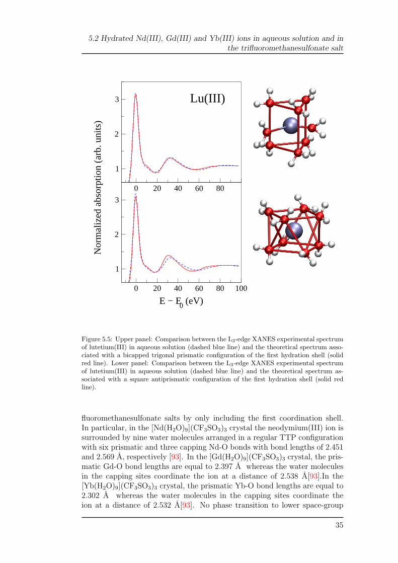
Figure 5.5: Upper panel: Comparison between the L3-edge XANES experimental spectrumof lutetium(III) in aqueous solution (dashed blue line) and the theoretical spectrum asso-ciated with a bicapped trigonal prismatic configuration of the first hydration shell (solidred line). Lower panel: Comparison between the L3-edge XANES experimental spectrumof lutetium(III) in aqueous solution (dashed blue line) and the theoretical spectrum as-sociated with a square antiprismatic configuration of the first hydration shell (solid redline).
fluoromethanesulfonate salts by only including the first coordination shell.In particular, in the [Nd(H2O)9](CF3SO3)3 crystal the neodymium(III) ion issurrounded by nine water molecules arranged in a regular TTP configurationwith six prismatic and three capping Nd-O bonds with bond lengths of 2.451and 2.569 A, respectively [93]. In the [Gd(H2O)9](CF3SO3)3 crystal, the pris-matic Gd-O bond lengths are equal to 2.397 A whereas the water moleculesin the capping sites coordinate the ion at a distance of 2.538 A[93].In the[Yb(H2O)9](CF3SO3)3 crystal, the prismatic Yb-O bond lengths are equal to2.302 A whereas the water molecules in the capping sites coordinate theion at a distance of 2.532 A[93]. No phase transition to lower space-group
35

5 Structures of solvated Nd(III), Gd(III), Yb(III) and Lu(III) in aqueoussolution and crystalline salts
0 50 100 150
0.5
1N
orm
aliz
ed a
bsor
ptio
n (a
rb. u
nits
)
0
0.5
1
Nor
mal
ized
abs
orpt
ion
(arb
. uni
ts)
0 50 100 150
0.5
1
Nor
mal
ized
abs
orpt
ion
(arb
. uni
ts)
0 50 100 150
E − E0 (eV)
0.5
1
1.5
Solid
Solid Solid Solid
Solution
Solution Solution Solution
SolidSolution
0 50 100 150
E − E0 (eV)
0.5
1
1.5
0 50 100 150
E − E0 (eV)
0.5
1
1.5
SolidSolution
Nd(III) Yb(III)Gd(III)
Figure 5.6: The upper panels of each figures show the comparison between the raw K-edge XANES spectra of neodimium(III), gadolinium(III) and ytterbium(III) in aqueoussolution (solid line) and in solid trifluoromethanesulfonate salts (red dotted line). Thelower panels show the comparison between the raw K-edge deconvolved XANES spectra ofneodimium(III), gadolinium(III) and ytterbium(III) in aqueous solution (solid line) and insolid trifluoromethanesulfonate salts (red dotted line).
symmetry was observed at low-temperature for the hydrated lanthanoid(III)trifluoromethanesulfonate salts with full occupancy in the capping positions.In Figure 5.7, the results of the minimization procedure applied to the K-edgeXANES raw and deconvolved data spectra of neodymium(III) aqueous solu-tion are reported. In these cases the agreement between the experimentaland theoretical data is very good, and the structural results compare verywell with the crystallographic metrics (see Table 5.1).
A different strategy has been used for the analysis of the XANES dataof gadolinium(III) and ytterbium(III) based on the results of a previous com-bined crystallographic and EXAFS investigation [15]. This study has shownthat for the medium-sized lanthanoid(III) ions (Sm-Ho) the mean cappingbond lengths from the EXAFS data are somewhat shorter than the crystal-lographic results with a full occupancy in the capping positions, while forthe heavy lanthanoid(III) ions (Er-Lu) water deficiency in the three cappingpositions starts at holmium(III) and increases for erbium(III), thulium(III),ytterbium(III) and lutetium(III). This deviation has been explained with theexistence of a slightly distorted molecular configuration, probably with onecapping water molecule that is more strongly bound to the ion. For this rea-son, the XANES spectra of the gadolinium(III) and ytterbium(III) ion havebeen analyzed by imposing the same prismatic Gd-O and Yb-O bond lengthswhile refining the three capping water molecules independently. For Gd thebest-fit structure obtained from the minimization resulted in a distorted TTPcomplex with one water molecule in the capping site coordinating the ion ata slightly shorter distance (2.49 A) as compared with the other two cappingmolecules (2.54 A), and for Yb a TTP complex with three different distancesof the capping sites (2.54, 2.44 and 2.39 A). Figures 5.8, 5.9 a) and 5.9 c)
36

5.2 Hydrated Nd(III), Gd(III) and Yb(III) ions in aqueous solution and inthe trifluoromethanesulfonate salt
0 50 100 150
0.5
1
Nor
mal
ized
abs
orpt
ion
(arb
. uni
ts)
0 50 100 150
E − E0 (eV)
0.5
1
1.5
Nd(III)
Figure 5.7: Upper panel: Comparison between the K-edge raw XANES experimental spec-trum of neodymium(III) in aqueous solution (dashed blue line) and the theoretical spec-trum including the first coordination shell, only (solid red line). Lower panel: Comparisonbetween the K-edge deconvolved XANES experimental spectrum of neodymium(III) inaqueous solution (dashed blue line) and the theoretical spectrum including the first coor-dination shell, only (solid red line)..
depict the comparison between the experimental (raw and deconvolved data)K-edge spectra of gadolinium(III) and the deconvolved K-edge only spectrumof ytterbium(III) in aqueous solution and the theoretical calculations. Theagreement is very good and the best-fit structure results are listed in Table5.1.
Very similar results were obtained for the three ions from the analysisof the solid trifluoromethanesulfonate salts (Table 5.1). The comparison ofthe L3-edges of the solid samples and aqueous solution shows remarkabledifferences (see Figure 5.10).
In particular, the intensity of the white line and the overall shape of thesespectra are different, and the quantitative analysis of the spectra allowed us,once more, to shed light on the origin of this phenomenon. Two different
37
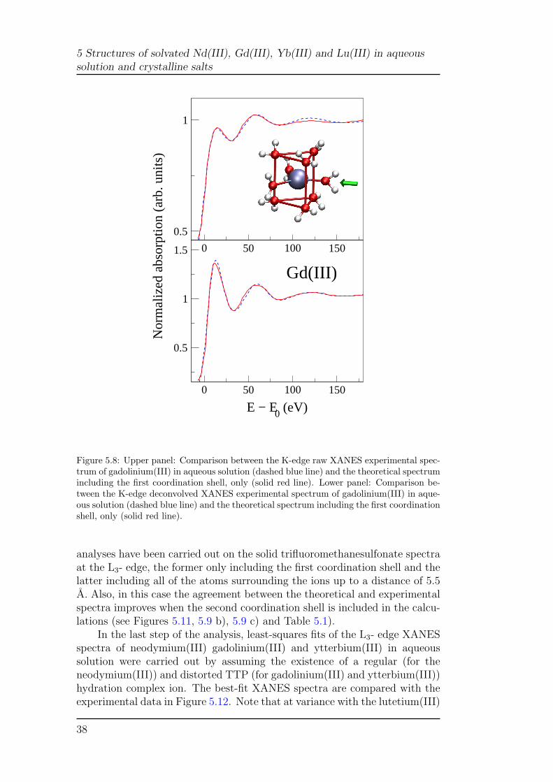
5 Structures of solvated Nd(III), Gd(III), Yb(III) and Lu(III) in aqueoussolution and crystalline salts
0 50 100 150
0.5
1
Nor
mal
ized
abs
orpt
ion
(arb
. uni
ts)
0 50 100 150
E − E0 (eV)
0.5
1
1.5
Gd(III)
Figure 5.8: Upper panel: Comparison between the K-edge raw XANES experimental spec-trum of gadolinium(III) in aqueous solution (dashed blue line) and the theoretical spectrumincluding the first coordination shell, only (solid red line). Lower panel: Comparison be-tween the K-edge deconvolved XANES experimental spectrum of gadolinium(III) in aque-ous solution (dashed blue line) and the theoretical spectrum including the first coordinationshell, only (solid red line).
analyses have been carried out on the solid trifluoromethanesulfonate spectraat the L3- edge, the former only including the first coordination shell and thelatter including all of the atoms surrounding the ions up to a distance of 5.5A. Also, in this case the agreement between the theoretical and experimentalspectra improves when the second coordination shell is included in the calcu-lations (see Figures 5.11, 5.9 b), 5.9 c) and Table 5.1).
In the last step of the analysis, least-squares fits of the L3- edge XANESspectra of neodymium(III) gadolinium(III) and ytterbium(III) in aqueoussolution were carried out by assuming the existence of a regular (for theneodymium(III)) and distorted TTP (for gadolinium(III) and ytterbium(III))hydration complex ion. The best-fit XANES spectra are compared with theexperimental data in Figure 5.12. Note that at variance with the lutetium(III)
38

5.2 Hydrated Nd(III), Gd(III) and Yb(III) ions in aqueous solution and inthe trifluoromethanesulfonate salt
0 20 40 60 80
1
1.5
2
Nor
mal
ized
abs
orpt
ion
(arb
. uni
ts)
1
1
st
st
shell
shell
0 50 100 150
0.5
1
1.5
Nor
mal
ized
abs
orpt
ion
(arb
. uni
ts)
0 20 40 60 80 100
E − E0 (eV)
1
1.5
21
1
st
st
and 2
and 2
nd
nd
shell
shell
0 50 100 150 200
E − E
b)
d)
a)
c)
0 (eV)
0.5
1
Figure 5.9: a) Comparison between the deconvolved K-edge XANES experimental spec-trum of solid [Yb(H2O)8.7](CF3SO3)3 (dotted blue line) and the best-fit theoretical spec-trum including only the first hydration sphere (solid red line); b) Comparison between theL3-edge XANES experimental spectrum of solid [Yb(H2O)8.7](CF3SO3)3 (dotted blue line)and the best-fit theoretical spectrum including only the first hydration sphere (solid redline); c) Comparison between the deconvolved K-edge XANES experimental spectrum ofsolid [Yb(H2O)8.7](CF3SO3)3 (dotted blue line) and the best-fit theoretical spectrum in-cluding both the first and second hydration shells (solid red line); d) Comparison betweenthe L3-edge XANES experimental spectrum of solid [Yb(H2O)8.7](CF3SO3)3 (dotted blueline) and the best-fit theoretical spectrum including both the first and second hydrationshells (solid red line).
0 50 100
E − EE − E 00 (eV) (eV)
0
1
2
50
3
100
Nor
mal
ized
abs
orpt
ion
(arb
. uni
ts)
SolidSolution
1
2
3
Nor
mal
ized
abs
orpt
ion
(arb
. uni
ts)
SolidSolution
0
E − E0 (eV)
0.5
1
1.5
2
Nor
mal
ized
abs
orpt
ion
(arb
. uni
ts)
SolidSolutionGd(III) Yb(III)Nd(III)
Figure 5.10: Comparison between the L3-edge XANES spectra of neodimium(III) (leftpanel), gadolinium(III)(middle panel) and ytterbium(III)(right panel) in aqueous solution(solid line) and in solid trifluoromethanesulfonate salts (red dotted line).
results, in this case it was not possible to perfectly reproduce the experimen-tal spectra by only using the first hydration shell cluster. This finding pointsout the need to include the second hydration shell in the XANES theoret-ical calculation to get a good agreement with the experimental data of theaqueous solution samples.
39

5 Structures of solvated Nd(III), Gd(III), Yb(III) and Lu(III) in aqueoussolution and crystalline salts
0 020 2040 4060 6080 80
1
0.5
2
1
3
1.5
Nor
mal
ized
abs
orpt
ion
(arb
. uni
ts)
2
Nor
mal
ized
abs
orpt
ion
(arb
. uni
ts)
11stst shell shell
00 20 4020 6040 8060 10080
E − E100
E − E 00 (eV) (eV)
1
2
3
0.5
1
1.5
2
1st
1 and 2st nd and 2 shellnd
shell
Nd(III) Gd(III)
Figure 5.11: Top left panel:Comparison between the L3 XANES experimental spectrumof solid [Nd(H2O)9](CF3SO3)3 (dashed blue line) and the theoretical spectrum includingthe first coordination shell, only (solid red line). Lower left panel: Comparison betweenthe L3 XANES experimental spectrum of solid [Nd(H2O)9](CF3SO3)3 (dashed blue line)and the theoretical spectrum including the first plus second coordination shells (solid redline). Top right panel: Comparison between the L3 XANES experimental spectrum of solid[Gd(H2O)9](CF3SO3)3 (dashed blue line) and the theoretical spectrum including the firstcoordination shell, only (solid red line). Lower right panel: Comparison between the L3
XANES experimental spectrum of solid [Gd(H2O)9](CF3SO3)3 (dashed blue line) and thetheoretical spectrum including the first plus second coordination shells (solid red line).
00 0 2020 20 4040 40 6060 60 8080 80 100100 100
E − EE − E E − E00 0 (eV) (eV) (eV)
0.5
1
1
2
1
1.5
3
1.5
2
Nor
mal
ized
abs
orpt
ion
(arb
. uni
ts)
2
Nor
mal
ized
abs
orpt
ion
(arb
. uni
ts)
2.5
Nor
mal
ized
abs
orpt
ion
(arb
. uni
ts)
Nd(III) Gd(III) Yb(III)
Figure 5.12: Comparison between the L3 XANES experimental spectrum ofneodymium(III)(left panel), gadolinium(III)(middle panel) and ytterbium(III)(right panel)in aqueous solution (dashed blue line) and the theoretical spectrum associated with a tri-capped trigonal prismatic configuration of the first hydration shell (solid red line).
40

5.2 Hydrated Nd(III), Gd(III) and Yb(III) ions in aqueous solution and inthe trifluoromethanesulfonate salt
Tab
le5.
1:K
-an
dL
3-e
dge
XA
NE
Sst
ruct
ural
para
met
ers
ofth
ehy
drat
edlu
teti
um(I
II),
neod
ymiu
m(I
II),
gado
liniu
m(I
II)
and
ytte
rbiu
m(I
II)
ions
inth
eso
lidtr
ifluo
rom
etha
nesu
lfona
tesa
lts
and
insl
ight
lyac
idic
aque
ous
solu
tion
s.Ln-
Op
isth
edi
stan
cebe
twee
nth
eio
nan
dth
esi
xeq
uiva
lent
oxyg
enat
oms
inth
epr
ism
atic
site
s,Ln-
Oc1,Ln-
Oc2,an
dLn-
Oc3
are
the
dist
ance
sbe
twee
nth
eio
nan
dea
chca
ppin
gox
ygen
atom
.D
ista
nces
are
inA
whi
leΓ
car
ein
eV.T
heE
XA
FS
dete
rmin
atio
nsar
ere
port
edfo
rco
mpa
riso
n.[1
5]
K-e
dge
dat
aL
3-e
dge
dat
aLn-O
pLn-O
c1Ln-O
c2Ln-O
c3Γ
cLn-O
pLn-O
c1Ln-O
c2Ln-O
3Γ
c
Lu(I
II)
trifl
uoro
meth
anesu
lfonate
(solid)
XA
NE
S2.
31(6
)2.
34(5
)2.
60(5
)25
.82.
28(2
)2.
34(3
)2.
59(3
)5.
0X
AN
ES
dec
2.27
(3)
2.33
(4)
2.61
(3)
9.8
EX
AFS
2.30
(1)
2.37
(2)∗
2.32
(4)
2.37
(4)∗
Lu(I
II)/
wate
rX
AN
ES
2.31
(5)
2.34
(5)
2.60
(5)
30.3
2.25
(3)
2.37
(2)
2.56
(3)
4.7
XA
NE
Sdec
2.26
(2)
2.33
(4)
2.61
(4)
10.0
EX
AFS
2.29
(1)
2.35
(2)∗
2.28
(4)
2.37
(4)∗
Nd(I
II)
trifl
uoro
meth
anesu
lfonate
(solid)
XA
NE
S2.
48(5
)2.
57(5
)2.
57(5
)2.
57(5
)15
.32.
44(2
)2.
56(2
)2.
56(2
)2.
56(2
)3.
7X
AN
ES
dec
2.44
(2)
2.56
(4)
2.56
(4)
2.56
(4)
2.5
EX
AFS
2.47
(1)
2.57
(2)∗
2.48
(4)
2.58
(4)∗
Nd(I
II)/
wate
rX
AN
ES
2.45
(5)
2.57
(5)
2.57
(5)
2.57
(5)
15.3
2.46
(2)
2.57
(2)
2.57
(2)
2.57
(2)
3.7
XA
NE
Sdec
2.44
(2)
2.56
(3)
2.56
(4)
2.56
(4)
2.9
EX
AFS
2.48
(1)
2.57
(2)∗
2.47
(4)
2.60
(4)∗
∗M
ean
cappin
gbon
dle
ngt
h
41

5 Structures of solvated Nd(III), Gd(III), Yb(III) and Lu(III) in aqueoussolution and crystalline salts
K-ed
gedata
L3 -ed
gedata
Ln-O
pLn-O
c1Ln-O
c2Ln-O
c3Γ
cLn-O
pLn-O
c1Ln-O
c2Ln-O
3Γ
c
Gd(III)
trifluoro
meth
anesu
lfonate
(solid
)X
AN
ES
2.39(4)2.54(5)
2.54(5)2.49(5)
20.42.39(2)
2.54(2)2.54(2)
2.49(2)4.7
XA
NE
Sdec
2.37(4)2.54(4)
2.54(4)2.49(4)
6.2E
XA
FS
2.41(1)2.53(2) ∗
2.41(4)2.35(4) ∗
Gd(III)/
wate
rX
AN
ES
2.37(6)2.54(5)
2.54(5)2.49(5)
19.92.40(4)
2.54(4)2.54(4)
2.49(5)3.7
XA
NE
Sdec
2.37(3)2.53(4)
2.53(4)2.47(4)
6.4E
XA
FS
2.41(1)2.55(2) ∗
2.40(4)2.53(4) ∗
Yb(III)
trifluoro
meth
anesu
lfonate
(solid
)X
AN
ES
2.30(2)2.54(2)
2.44(2)2.39(2)
5.0X
AN
ES
dec
2.26(4)2.54(4)
2.44(4)2.39(4)
4.6E
XA
FS
2.32(1)2.46(2) ∗
2.32(4)2.43(4) ∗
Yb(III)/
wate
rX
AN
ES
2.30(4)2.54(4)
2.44(4)2.39(5)
4.0X
AN
ES
dec
EX
AFS
2.31(4)2.43(4) ∗
∗M
eancap
pin
gbon
dlen
gth
42

5.2 Hydrated Nd(III), Gd(III) and Yb(III) ions in aqueous solution and inthe trifluoromethanesulfonate salt
Tab
le5.
2:N
on-s
truc
tura
lpa
ram
eter
sas
dete
rmin
edby
MX
AN
.E
F(e
V)
isth
eFe
rmi
ener
gyle
vel,
Es
(eV
)is
the
plas
mon
ener
gy,
As
isth
epl
asm
onam
plit
ude,
E0
(eV
)is
the
thre
shol
den
ergy
,an
dΓ
exp
(eV
)is
the
expe
rim
enta
lre
solu
tion
.
K-e
dge
dat
aL
3-e
dge
dat
aE
FE
s 1A
s 1E
s 2A
s 2E
0Γ
exp
EF
Es 1
As 1
E0
Γex
p
Lu(I
II)
trifl
uoro
meth
anesu
lfonate
(solid
incl
udin
gth
efirs
tco
ord
inati
on
shell
only
)3.
56.
010
.215
.213
.85.
41.
0-1
.080
.080
.05.
72.
2D
EC
-2.7
25.1
3.2
1.2
2.3
Lu(I
II)
trifl
uoro
meth
anesu
lfonate
(solid
incl
udin
gboth
the
firs
tand
the
seco
nd
coord
inati
on
shell)
-1.0
79.7
80.0
5.7
2.2
Lu(I
II)/
wate
r5.
18.
112
.410
.39.
85.
01.
0-1
.875
.080
.05.
11.
2D
EC
-1.8
26.8
1.0
-1.4
2.3
Nd(I
II)
trifl
uoro
meth
anesu
lfonate
(solid
incl
udin
gth
efirs
tco
ord
inati
on
shell
only
)-4
.81.
427
.522
.55.
3-5
.01.
1-1
.021
.912
.25.
72.
1D
EC
-3.3
14.8
6.3
-2.1
2.0
Nd(I
II)
trifl
uoro
meth
anesu
lfonate
(solid
incl
udin
gboth
the
firs
tand
the
seco
nd
coord
inati
on
shell)
-1.0
21.9
12.2
5.7
2.1
Nd(I
II)/
wate
r-3
.12.
344
.319
.64.
50.
21.
1-7
.715
.36.
26.
40.
8D
EC
-3.3
14.8
6.3
-2.1
1.8
43

5 Structures of solvated Nd(III), Gd(III), Yb(III) and Lu(III) in aqueoussolution and crystalline salts
K-ed
gedata
L3 -ed
gedata
EF
Es1
As1
Es2
As2
E0
Γex
pE
FE
s1
As1
E0
Γex
p
Gd(III)
trifluoro
meth
anesu
lfonate
(solid
inclu
din
gth
efirst
coord
inatio
nsh
ell
only
)2.6
2.833.7
40.55.5
-1.11.0
-7.315.1
4.63.8
0.8D
EC
-2.825.3
8.6-4.3
1.6G
d(III)
trifluoro
meth
anesu
lfonate
(solid
inclu
din
gboth
the
first
and
the
seco
nd
coord
inatio
nsh
ell)
-0.815.1
4.63.8
0.8G
d(III)/
wate
r-2.8
20.433.7
2.840.6
0.41.0
-9.928.8
17.94.6
1.3D
EC
-5.721.5
7.5-1.8
2.0
Yb(III)
trifluoro
meth
anesu
lfonate
(solid
inclu
din
gth
efirst
coord
inatio
nsh
ell
only
)-1.2
7.96.6
4.02.3
DE
C0.0
15.22.4
-2.84.5
Yb(III)
trifluoro
meth
anesu
lfonate
(solid
inclu
din
gboth
the
first
and
the
seco
nd
coord
inatio
nsh
ell)
-1.27.9
6.64.0
2.3D
EC
2.210.0
6.0-2.8
4.3Y
b(III)/
wate
r-9.9
15.210.1
4.22.7
44

Chapter 6
Structural and dynamicproperties of neodymium(III),gadolinium(III) andytterbium(III) ions in aqueoussolution
6.1 Molecular Dynamic simulations
The structural properties of the three aqueous solution are described interms of the metal-oxygen and metal-hydrogen radial distribution functionsor g(r)’s [59]:
gAB(r) =〈ρB(r)〉〈ρB〉local
=1
NA〈ρB〉local
NA∑i∈A
NB∑j∈B
δ(rij − r)
4πr2(6.1)
where 〈ρB(r)〉 is the particle density of type B at a distance r around particlesA, 〈ρB〉local is the particle density of type B averaged over all the spheresaround particles A with radius rmax (which is equal to half of the box side),NA and NB is the number of A and B particles, and rij is the distance betweeni (of type A) and j (of type B) particles. Therefore, an average over time andover the A particles is performed in the gAB(r) calculation. The Ln-O andLn-H g(r)’s obtained from the MD simulations are shown in Figure 6.1 whilethe main structural results are collected in Table 6.1. The first peak positionsof the g(r)’s show the expected lanthanoid contraction with an elongation ofthe first hydration shell going from Yb(III) to Nd(III). Inspection of Table6.1 reveals that the first maximum positions of the present simulations areshorter than those obtained from Floris et al. (see Table 3 of ref [5]) and are inbetter agreement with the experimental results. The shortening of the Ln-Ofirst shell distance could be due to the larger box size used in our simulationswhich allows a better treatment of the ion-solvent interactions. However, adirect proof of the reliability of the MD simulations has been obtained by
45

6 Structural and dynamic properties of neodymium(III), gadolinium(III)and ytterbium(III) ions in aqueous solution
comparison with EXAFS experimental data.
3 4 50
5
10
15Nd
3 4 50
5
10
15
g(r)
Gd
3 4 5
r(Å)
0
5
10
15
Yb
Figure 6.1: Ln-O (red line) and Ln-H (black line) radial distribution functions obtainedfor aqueous solutions of Nd(III), Gd(III), and Yb(III) from MD simulations.
Table 6.1: Positions (in A) at maxima of Ln-O and Ln-H g(r)’s.
Nd-O Nd-H Gd-O Gd-H Yb-O Yb-H
First Maxima
Floris et al.[5] 2.53 3.18 2.46 3.10 2.37 3.02This work 2.48 3.15 2.43 3.09 2.32 2.99
Second Maxima
Floris et al.[5] 4.58 5.01 4.50 4.94 4.41 4.93This work 4.54 5.01 4.50 4.93 4.38 4.91
46

6.2 EXAFS Analysis
6.2 EXAFS Analysis
A direct comparison between MD and EXAFS results can be performed bycalculating the χ(k) theoretical signal associated with the MD Ln-O and Ln-H g(r)’s by means of equation 2.5 and by comparing it with the experimentalspectrum, without carrying out any minimization procedure. Here, we haveused the K-edge spectra of Ln(III) ions in aqueous solutions as it has beenshown that the K-edge EXAFS data provide more accurate structural resultsas compared to the L3-edge ones [41]. In the upper panels of Figure 6.2the comparison between the EXAFS experimental signal and the theoreticalcurves calculated using the MD g(r)’s is reported for the Nd(III), Gd(III), andYb(III) ions. The first two curves from the top of each panel are the two-bodyLn-O and Ln-H first shell contributions (γ(2)) while the remainder of the figureshows the total theoretical contributions compared with the experimentalspectra and the resulting residuals. The γ(2) signals are shown multipliedby k2 for better visualization. As expected, the dominant contribution tothe total EXAFS spectrum is given by the Ln-O first shell signal and, asa consequence, the EXAFS structural information is particularly accuratefor the shape of the Ln-O g(r)’s first peaks, only. The Fourier transform(FT) moduli of the EXAFS χ(k)k2 theoretical, experimental, and residualsignals are shown in the lower panels of Figure 6.2. The FT’s have beencalculated in the k-range 3.5-15.0 A−1 with no phase shift correction applied.The FT spectra show a prominent first shell peak which is mainly due tothe Ln-O first shell distance. Nevertheless, the Ln-H FT peaks are locatedat about 2.4 A, giving rise to a shoulder on the first peak. Overall, thecalculated EXAFS spectra match the experimental data reasonably well inall cases showing that the structural and dynamical information derived fromthe MD simulations is basically correct and that the SPC/E water modelprovides reliable values for the ion-water distances. However, in the case ofthe Yb(III) ion, the agreement is slightly worse, and the residual curve showsthe presence of a spurious leading frequency. This small mismatch betweenthe experimental and theoretical curves reflects the lower accuracy of theYb(III) MD simulation, as already pointed out by Floris et al [5].
6.3 XANES Analysis
As previously mentioned the quantitative XANES analysis of aqueoussolutions can be carried out only if the structural disorder within the first hy-dration shell and the contribution of the higher distance coordination spheresare properly accounted for [39, 94, 40, 78, 36]. As far as the K-edge spectra areconcerned, the close similarity of the solid [Ln(H2O)9](CF3SO3)3 and Ln(III)aqueous solution XANES spectra (see Figure 5.6) suggests a substantial in-sensitivity toward the second coordination sphere. We have therefore decidedto focus our attention on the L3-edge spectra in water. The left panel ofFigure 6.3 shows the averaged theoretical spectrum obtained from 500 snap-shots (not including intrinsic and extrinsic inelastic process) associated with
47

6 Structural and dynamic properties of neodymium(III), gadolinium(III)and ytterbium(III) ions in aqueous solution
Figure 6.2: Analysis of the K-edge EXAFS spectra of aqueous solutions of Nd(III) (leftpanel), Gd(III) (middle panel), and Yb(III) (right panel) starting from the Ln-O and Ln-Hradial distribution functions obtained from MD simulations. From the top to the bottomof each panel, the following curves are reported: the Ln-O first shell signals, the Ln-H firstshell signals, the total theoretical signals compared with the experimental spectrum, andthe residual curves. The lower panels show the nonphase-shift-corrected Fourier transformsof the experimental data (dotted line), of the total theoretical signals (full line), and of theresidual curves (dashed-dotted line).
the first hydration shell of the hydrated Yb(III) ion, together with severalindividual instantaneous structures. The calculated XANES spectra presentnoticeable differences all along the energy range, showing the sensitivity ofXANES to geometrical changes, and the importance of making a proper sam-pling of the configurational space. As far as the second shell is concerned ourMD simulation suggests the presence of 27 water molecules up to about 6.0A from the Yb(III) ion. The XANES total theoretical spectrum obtainedfrom 500 MD snapshots including both the first- and second-shell is shownin the right panel of Figure 6.3, together with several spectra computed frominstantaneous configurations. In this case the individual spectra show moremarked differences as compared to the first hydration shell. Considering thelarge deviation among instantaneous spectra it seems unlikely that a singlerepresentative configuration can be used to properly model the experimentaldata.
To better highlight the influence of the second hydration shell on the L3-edge XANES spectrum of the Yb(III) ion in aqueous solution it is useful to
48

6.3 XANES Analysis
Figure 6.3: Left panel: Comparison of the theoretical XANES spectrum of the Yb(III)ion in water obtained from the MD average including only the first hydration shell (redline) and several spectra associated with individual MD configurations (black lines). Rightpanel: Comparison of the theoretical XANES spectrum of the Yb(III) ion in water obtainedfrom the MD average including both the first and second hydration shells (red line) andseveral spectra associated with individual MD configurations (black lines).
compare the averaged spectrum calculated using first-shell-only and first- andsecond-shell clusters (see Figure 6.4). The calculated XANES spectra presentnoticeable differences in the energy range up to 50 eV from the threshold. Inparticular, the edge intensity is lowered in the spectrum containing only thefirst shell water molecules, which exhibits a different shape in the regionaround the first minimum. The two spectra become identical for energy val-ues higher than 60 eV, and this finding underlines the insensitivity of theEXAFS technique toward second shell contributions.
To assess the reliability of our results it is necessary to compare thetotal averaged XANES spectra with the experimental data. To this end allinelastic processes have been accounted for by convoluting the theoreticalaveraged spectra with a broadening Lorentzian function (see equation 2.8),and the corresponding Es and A non-structural parameters (see section 2.3)have been optimized (see Table6.2). In the upper panel of Figure 6.5, theexperimental XANES data of the Yb(III) ion in water are compared withthe averaged theoretical spectrum including the first-shell clusters as derivedfrom MD simulations. The overall agreement of the two spectra is not per-fect in the entire energy range. In the lower panel Figure 6.5, the averagedtheoretical spectrum including both the first and second hydration shells iscompared with the experimental data. In this case, the agreement betweenthe experimental and theoretical spectra is very good, the intensity of thewhite line is recovered and the shape of the first minimum region is very sim-ilar to the experimental data. It is important to remark that all the XANES
49

6 Structural and dynamic properties of neodymium(III), gadolinium(III)and ytterbium(III) ions in aqueous solution
Figure 6.4: Comparison of the L3-edge theoretical XANES spectrum obtained from theMD average including only the first hydration shell (solid line) and the averaged theoreticalXANES spectrum including both the first and second shells (dashed line).
spectra have been calculated using the structural information obtained fromthe MD simulations without carrying out any minimization in the structuralparameter space. Because of the high sensitivity of the XANES techniquetoward the structural environment of the photoabsorber this approach is avery strict test on the quality of the potentials used in the MD simulations,and the almost perfect agreement between the averaged theoretical and ex-perimental XANES spectra proves the reliability of the entire computationalprocedure.
A complete picture of the potentiality of the XANES technique for thestructural characterization of lanthanoid solutions has been obtained by an-alyzing the L3-edge XANES spectra of two additional ions, namely, Nd(III)and Gd(III). The analysis of the aqueous solution XANES spectra has beencarried out along the line of the Yb(III) ion. Figure 6.6 shows the compar-ison between the averaged theoretical spectra computed on the basis of theMD trajectories and the experimental data. The analysis including only thefirst hydration shells is reported in the upper panels while the averaged the-oretical spectra computed including all the water molecules up to 6 A areshown in the lower panels. Note that for both ions the agreement betweenthe experimental and theoretical data improves when the second hydrationshell is taken into account. Also in this case the inclusion of the higher dis-tance ligands produces additional features that are clearly detectable in the
50

6.3 XANES Analysis
0 20 40 60 80
1
1.5
2
2.5
Nor
mal
ized
abs
orpt
ion
1st shell
0 20 40 60 80 100
E − E0 (eV)
1
1.5
2 1st and 2
nd shell
Figure 6.5: Upper panel: Comparison between the L3-edge XANES experimental spectrumof Yb(III) aqueous solution (dotted blue line) and the MD averaged theoretical spectrumincluding only the first coordination sphere (solid red line). Lower panel: Comparisonbetween the L3-edge XANES experimental spectrum of the Yb(III) ion in aqueous solution(dotted blue line) and the MD averaged theoretical spectrum including both the first andsecond coordination shell (solid red line).
experimental data.Finally, we have used the instantaneous configurations of the MD simula-
tions to compute K-edge averaged XANES spectra for the three ions. In thiscase we have included only the first shell water molecules, and the compari-son with the deconvolved experimental spectra is shown in Figure 6.7. Theagreement between the experimental and theoretical spectra is quite goodfor all the three ions, proving simultaneously the reliability of the procedureand the insensitivity of the K-edge XANES spectra toward higher distancecoordination shells.
51

6 Structural and dynamic properties of neodymium(III), gadolinium(III)and ytterbium(III) ions in aqueous solution
0 20 400 60 8020 40 60 80
1
2
1
3
2N
orm
aliz
ed a
bsor
ptio
n
3
4
Nor
mal
ized
abs
orpt
ion
1st
1 shell st shell
0 200 40 6020 8040 10060
E − E80 100
0E − E (eV)0 (eV)
11
22
3
3
1 1st st and 2 and 2
nd nd shell shell
Gd(III)Nd(III)
a) b)
c) d)
Figure 6.6: a) Comparison between the L3-edge XANES experimental spectrum of theNd(III) ion in aqueous solution (dotted blue line) and the MD averaged theoretical spec-trum including only the first hydration sphere (solid red line); b) Comparison between theL3-edge XANES experimental spectrum of the Gd(III) ion in aqueous solution (dotted blueline) and the MD averaged theoretical spectrum including only the first hydration sphere(solid red line); c) Comparison between the L3-edge XANES experimental spectrum of theNd(III) ion in aqueous solution (dotted blue line) and the MD averaged theoretical spec-trum including both the first and second hydration shells (solid red line); d) Comparisonbetween the L3-edge XANES experimental spectrum of the Gd(III) ion in aqueous solution(dotted blue line) and the MD averaged theoretical spectrum including both the first andsecond hydration shells (solid red line).
52
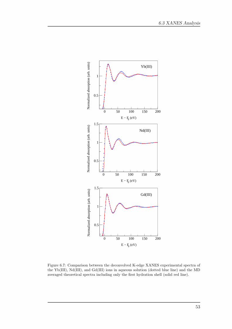
6.3 XANES Analysis
0 50 100 150 200
E − E0 (eV)
0 50 100
0.5
150
1
200
0
1.5
E − E
Nor
mal
ized
abs
orpt
ion
(arb
. uni
ts)
50
0
100 150
(eV)
200
E − E0 (eV)
0.5
1
1.5
Nor
mal
ized
abs
orpt
ion
(arb
. uni
ts)
0.5
1
Nor
mal
ized
abs
orpt
ion
(arb
. uni
ts)
Gd(III)
Nd(III)
Yb(III)
Figure 6.7: Comparison between the deconvolved K-edge XANES experimental spectra ofthe Yb(III), Nd(III), and Gd(III) ions in aqueous solution (dotted blue line) and the MDaveraged theoretical spectra including only the first hydration shell (solid red line).
53

6 Structural and dynamic properties of neodymium(III), gadolinium(III)and ytterbium(III) ions in aqueous solution
Table
6.2:N
on-structuralparam
etersas
determined
byM
XA
Nfrom
MD
simulations.
EF
(eV)
isthe
Fermienergy
level,E
s(eV
)is
theplasm
onenergy,
As
isthe
plasmon
amplitude,
E0
(eV)
isthe
thresholdenergy,
andΓ
exp
(eV)
isthe
experimental
resolution.
L3 -ed
gedata
K-ed
gedecon
volveddata
EF
Es
As
E0
Γex
pE
FE
sA
sE
0Γ
exp
Nd(III)/
wate
r(fro
mM
Dw
ithfirst
shell
only
)-7.9
14.32.3
0.76.5
-7.38.7
5.62.2
2.9N
d(III)
wate
r(fro
mM
Dw
ithfirst
and
seco
nd
shell)
-9.014.6
3.60.7
2.2
Gd(III)/
wate
r(fro
mM
Dw
ithfirst
shell
only
)-8.6
15.45.4
1.24.3
-14.95.3
6.02.4
1.9G
d(III)
wate
r(fro
mM
Dw
ithfirst
and
seco
nd
shell)
-10.025.0
6.61.6
2.3
Yb(III)/
wate
r(fro
mM
Dw
ithfirst
shell
only
)-7.7
18.03.8
1.64.2
-14.010.7
2.08.1
4.2Y
b(III)
wate
r(fro
mM
Dw
ithfirst
and
seco
nd
shell)
-9.116.8
4.01.6
1.2
54

Chapter 7
Polarized Simulation Results
7.1 Combined EXAFS and MD simulation
analysis
Recently Duvail et all. carried out polarized MD simulations of lanthanoidions in aqueous solution in which the Ln-O interaction potentials have beenbuilt up on the basis of Shannon ionic radius of each element (see section4.3). That ionic radii, in solid phase, reported by Shannon are a function ofthe number of oxygen atoms around the lanthanoid. As reference was takenthe La(III) ionic radius corresponding to a ninefold structure, i.e., 1.216 A,and for the other lanthanoids was taken the ninefold values for the lighterones and both ninefold and eightfold values for heavier atoms. Thus we havefor each Ln(III) heavier than Pm(III) a double set of simulations.Figure 7.1 shows the Ln-O bond distances obtained from the MD simulationsin comparison with the EXAFS results of a previous investigation [15]. All thestructural results are collected in Table 7.1. For the largest ions, Ln=La-Pr,the MD Ln-O bond distances are shorter than the EXAFS results, while fromNd(III) to Gd(III) the MD and EXAFS structural parameters are, within es-timated limits of error, in good agreement. Starting at Tb(III) up to Yb(III),the EXAFS bond distances place between the MD results for a nine and aneight coordination geometry, while for Lu(III) the EXAFS and MD simula-tion results for an eight coordination arrangement agree. On the basis ofthese results, we propose a new set of lanthanoids ionic radii in water (seeTable 7.2) as the Shannon ionic radius plus an additional term given by thedifference between EXAFS and MD simulation Ln-O bond distances:
Radiusnew = RadiusShannon + [(Ln − OEXAFS) − (Ln − OMD)] (7.1)
In Figure 7.2 the new ionic radii, togheter with the Shannon ionic radii, forall the lanthanoid series are plotted. The use of the new set of ionic radiiallowed to obtain MD simulations Ln-O bond distances that are in a verygood agreement with the EXAFS results, as shown in Figure 7.3 and reportedin Table 7.1.
55

7 Polarized Simulation Results
La Ce Pr Nd Pm Sm Eu Gd Tb Dy Ho Er Tm Yb Lu
2.35
2.4
2.45
2.5
2.55
2.6
2.65
2.7
d(Ln
-O)/
Å
DM Shannon 8DM Shannon 9EXAFS
Figure 7.1: Ln-O bond distances obtained from the MD simulation using a ninefold valuesof the Shannon ionic radius (green squares) and an eightfold values of the Shannon ionicradius (blue circles), while the Ln-O mean bond distances obtained from EXAFS [15] aremarked with red diamonds.
As previously done in section 6.2 a direct comparison between MD andEXAFS results can be performed by calculating the χ(k) theoretical signalassociated with the MD Ln-O and Ln-H g(r)’s and by comparing it with theexperimental spectrum, without carrying out any minimization procedure.For this analysis we selected four ions, Pr(III), Eu(III), Er(III) and Lu(III)as representative of the structural changes along the series. In Figure 7.4the comparison between the EXAFS experimental signal and the total the-oretical curves calculated using the MD g(r)’s is reported for Pr(III). In theupper section of the figure is shown the comparison between the total theo-retical signal obtained from the MD g(r)’s using the Shannon ionic radius fora ninefold coordination (SIR-9) with the experimental spectrum, while in thelower section is reported the same comparison but with a total theoreticalsignal obtained from the MD g(r)’s using our new ionic radius (NRI). It isclear that the use of the new ionic radii leads to a substantial improvementin the agreement between theoretical and experimental data. In the case ofEu(III) the better agreement between the EXAFS experimental and theoret-ical spectra is for a nine coordinated structure using a Shannon ionic radii,that in this case coincides with the radius proposed by us (Figure 7.5), whilefor Er(III) the best agreement is with the use of our new ionic radius (Figure
56

7.1 Combined EXAFS and MD simulationanalysis
La Ce Pr Nd Pm Sm Eu Gd Tb Dy Ho Er Tm Yb Lu
1
1.05
1.1
1.15
1.2
1.25
1.3Io
nic
Rad
ii (Å
)Shannon-9Shannon-8New
Figure 7.2: Ionic radii of the lanthanoid series in water solution as given by Shannon for aninefold structure (green squares), an eightfold strucure (blue circles) and the new set ofionic radii as determined by the EXAFS and MD polarized simulations (red diamonds)
7.6). For the last element of the lanthanoid series, namely the Lu(III), theEXAFS experimental data are well reproduced with a MD simulation usinga Shannon ionic radius corresponding to an eightfold structure (Figure 7.7).
57

7 Polarized Simulation Results
La Ce Pr Nd Pm Sm Eu Gd Tb Dy Ho Er Tm Yb Lu
2.35
2.4
2.45
2.5
2.55
2.6
2.65
2.7
d(Ln
-O)/
Å
DM Shannon 8DM Shannon 9EXAFSDM new radii
Figure 7.3: A summary of the results given in Table 7.1 of the lanthanoid(III) ions inaqueous solution as determined by EXAFS [15] and polarized MD simulations. The Ln-Obond distances obtained from the MD simulation using a ninefold values of the Shannonionic radius and an eightfold values of the Shannon ionic radius are marked with greensquares and blue circles respectively, the Ln-O mean bond distances obtained from EXAFSare marked with red diamonds, while the Ln-O bond distances obtained from the MDsimulations using the new set of ionic radii are marked with black circles.
58
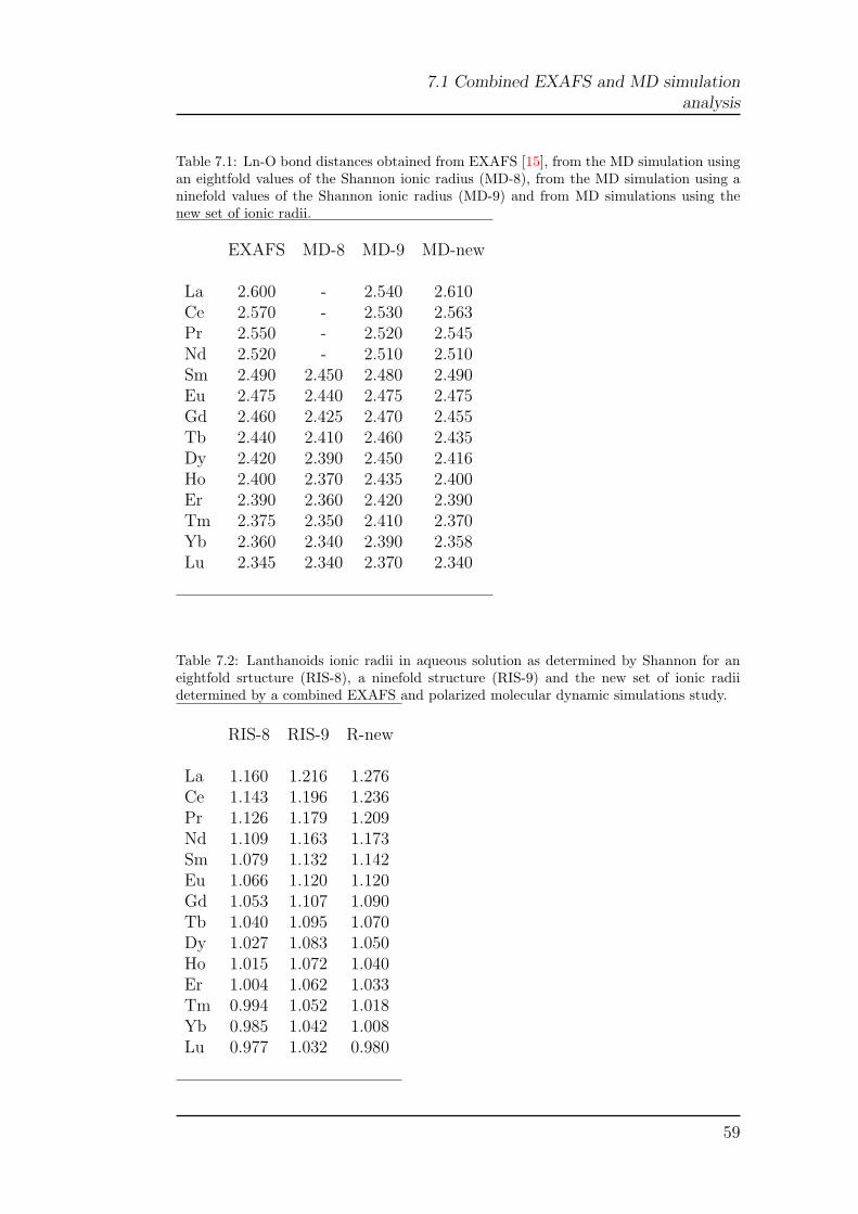
7.1 Combined EXAFS and MD simulationanalysis
Table 7.1: Ln-O bond distances obtained from EXAFS [15], from the MD simulation usingan eightfold values of the Shannon ionic radius (MD-8), from the MD simulation using aninefold values of the Shannon ionic radius (MD-9) and from MD simulations using thenew set of ionic radii.
EXAFS MD-8 MD-9 MD-new
La 2.600 - 2.540 2.610Ce 2.570 - 2.530 2.563Pr 2.550 - 2.520 2.545Nd 2.520 - 2.510 2.510Sm 2.490 2.450 2.480 2.490Eu 2.475 2.440 2.475 2.475Gd 2.460 2.425 2.470 2.455Tb 2.440 2.410 2.460 2.435Dy 2.420 2.390 2.450 2.416Ho 2.400 2.370 2.435 2.400Er 2.390 2.360 2.420 2.390Tm 2.375 2.350 2.410 2.370Yb 2.360 2.340 2.390 2.358Lu 2.345 2.340 2.370 2.340
Table 7.2: Lanthanoids ionic radii in aqueous solution as determined by Shannon for aneightfold srtucture (RIS-8), a ninefold structure (RIS-9) and the new set of ionic radiidetermined by a combined EXAFS and polarized molecular dynamic simulations study.
RIS-8 RIS-9 R-new
La 1.160 1.216 1.276Ce 1.143 1.196 1.236Pr 1.126 1.179 1.209Nd 1.109 1.163 1.173Sm 1.079 1.132 1.142Eu 1.066 1.120 1.120Gd 1.053 1.107 1.090Tb 1.040 1.095 1.070Dy 1.027 1.083 1.050Ho 1.015 1.072 1.040Er 1.004 1.062 1.033Tm 0.994 1.052 1.018Yb 0.985 1.042 1.008Lu 0.977 1.032 0.980
59

7 Polarized Simulation Results
Figure 7.4: Analysis of the K-edge EXAFS spectra of aqueous solution of Pr(III) startingfrom the Ln-O and Ln-H radial distribution functions obtained from MD polarized simula-tions. From the top to the bottom of the panel the following curves are reported: the totaltheoretical signals (red lines) compared with the experimental spectrum (black dotted line)and the residual curves (blue dotted line) related to the use of a Shannon ionic radius fora ninefold coordination (SIR-9) and the use of the new ionic radius (NIR).
60
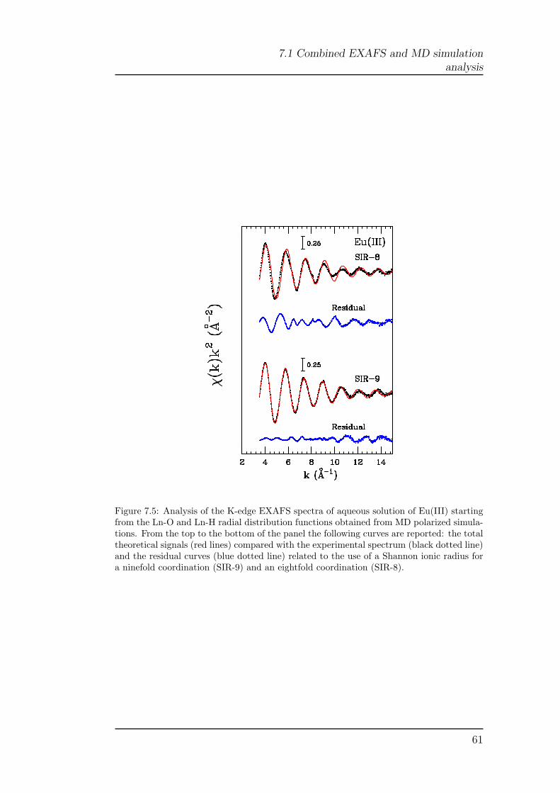
7.1 Combined EXAFS and MD simulationanalysis
Figure 7.5: Analysis of the K-edge EXAFS spectra of aqueous solution of Eu(III) startingfrom the Ln-O and Ln-H radial distribution functions obtained from MD polarized simula-tions. From the top to the bottom of the panel the following curves are reported: the totaltheoretical signals (red lines) compared with the experimental spectrum (black dotted line)and the residual curves (blue dotted line) related to the use of a Shannon ionic radius fora ninefold coordination (SIR-9) and an eightfold coordination (SIR-8).
61

7 Polarized Simulation Results
Figure 7.6: Analysis of the K-edge EXAFS spectra of aqueous solution of Er(III) startingfrom the Ln-O and Ln-H radial distribution functions obtained from MD polarized simula-tions. From the top to the bottom of the panel the following curves are reported: the totaltheoretical signals (red lines) compared with the experimental spectrum (black dotted line)and the residual curves (blue dotted line) related to the use of a Shannon ionic radius for aninefold coordination (SIR-9), an eightfold coordination (SIR-8) and the new ionic radius(NIR).
62

7.1 Combined EXAFS and MD simulationanalysis
Figure 7.7: Analysis of the K-edge EXAFS spectra of aqueous solution of Lu(III) startingfrom the Ln-O and Ln-H radial distribution functions obtained from MD polarized simula-tions. From the top to the bottom of the panel the following curves are reported: the totaltheoretical signals (red lines) compared with the experimental spectrum (black dotted line)and the residual curves (blue dotted line) related to the use of a Shannon ionic radius fora ninefold coordination (SIR-9) and an eightfold coordination (SIR-8).
63

7 Polarized Simulation Results
64

Chapter 8
Summary and conclusions
Previous experimental and theoretical works have shown that the hy-dration properties of the lanthanoid(III) ions are not so well established asassumed in the past years.[14, 16, 17, 15] In this paper, we have carried out aquantitative analysis of the K- and L3-edge XANES spectra of Ln(III) ions inaqueous solution which was able to catch crucial structural properties of thehydration complexes along the lanthanoid series. The XANES spectroscopyhas been found to be a very effective probe of the geometric structure oflanthanoid hydration clusters both in solid crystals and in aqueous solution.Across the series we observed a reduction of the coordination number, inthe form of a progressive mean departure of a water molecule from the cap-ping sites of the TTP prism, in agreement with the overall picture recentlyproposed on the basis of EXAFS results.[15] Changing the atom along theseries one of the capping water molecules is less and less strongly bound tothe Ln(III) ion, finally leaving the hydration complex. This gives rise to aneight-coordinated distorted bicapped trigonal prism with two different Ln-Ocapping distances for the last members of the series, as also observed for thehydrated scandium(III) ion.[33] It is important to stress that the XANEStechnique has allowed us to gain direct structural information on the exactgeometry of the coordination polyhedron of the hydrated Ln(III) ions, that isachievable neither by EXAFS nor by crystallography. Due to different reasonsboth these techniques fail in providing an unambiguous high-temperature de-termination of the coordination geometry of the hydrated lanthanoid species.In the case of disordered systems the accuracy of the structural determinationobtained by EXAFS can be inconclusive due to the well known limitationsof this technique to determine coordination numbers and the geometry ofpolyhedral environments. Moreover, when dealing with distorted TTP com-plexes, the loosely bound atoms in the capping positions contribute less tothe EXAFS signal, so that the bond-length determined by EXAFS is shorterthan the true mean value. On the other hand, the crystallographic structuresof Ln(III) hydrated trifluoromethanesulfonates at ambient temperature re-veal that the occupancy of the capping sites decreases with increasing atomicnumber. When one of the capping molecules is absent, there is a displace-ment of the metal ion from the center of the prism towards the two remaining
65

8 Summary and conclusions
capping waters which gives rise to distorted TTP geometries. This distortionis not detected by crystallography at room temperature as the high symme-try (P63/m) of the crystal structure is an average corresponding to a randomorientation of the capping water molecules. Therefore, the capping bond dis-tance obtained from x-ray diffraction is the mean value of two different setsof distances.
It is important to stress that the existence of distorted configurations ofthe the hydrated ion has been found in the low-temperature (100K) crystalstructure of [Lu(H2O)8.2](CF3SO3)3 and [Sc(H2O)8.0](CF3SO3)3.[15, 33] As aresult neither the EXAFS nor the crystallographic technique alone are able toprovide a true picture of the geometry of the hydrated lanthanoid ions, while areliable description of the structural change along the series has been obtainedfrom the comparison of the results obtained from the two techniques.[15]
An interesting issue which emerged from this study is the different resultsobtained from the analysis of the K- and L3-edge XANES spectra. In allcases the K-edge XANES spectra have been found to be insensitive to thesecond coordination shell. This is due to the very short lifetime of the ex-cited atomic state for absorption edges above 30 keV which gives rise to astrong damping and broadening of the signal. This affects in particular thehigh-frequency components of the measured signal and consequently reducesthe sensitivity of the technique to the more distant coordination shells. Notethat the K-edge XANES spectra of the aqueous solution samples and tri-fluoromethanesulfonate solid salts are always identical, thus proving on theone hand that the different second coordination shells are not probed, on theother that the coordination of the first hydration shell is equal in water andin the solid.
An additional conclusion can be drawn comparing the L3-edge XANESspectra of the three metal ions in aqueous solution. In the case of thelutetium(III) ion the second hydration shell has been found to provide anegligible contribution to the XANES spectrum. On the contrary, the neody-mium(III), gadolinium(III) and ytterbium(III) XANES spectra of the solutioncould not be reproduced using the well-established TTP first hydration shellonly, thus showing the need of including additional shells in the calculation.This finding can be explained by the different ionic radii, and consequentlyligand properties, of the three ions. With decreasing size of the Ln(III) ion therepulsion between the prism and capping water molecules increases giving riseto a progressive weakening of the interaction between the central metal andthe outer water molecules. As a consequence the occupancy of the cappingsites decreases along the series until on average almost one water moleculedeparts in the last members of the series. The inability of the ion to keepthe capping water molecules bound is also responsible for a reduced ability tostructure water. As a result the second hydration shell is more mobile withincreasing ionic size, becoming hardly observable in the XANES spectra.
In conclusion, we show that XANES is a very profitable tool to gain di-rect structural information on the coordination geometry of metal complexeswith low symmetry as the hydrated lanthanoid(III) ions, that is not achiev-
66

able by other experimental techniques. The results of this investigation pavethe route for the use of XANES for structural investigations of solid and liq-uid systems of metal ions with low symmetry, such as the actinoid series [95]and a wide class of metal-containing proteins [96, 97, 98] .
67

8 Summary and conclusions
68

Bibliography
[1] D.T. RichensThe chemistry of aqua ions John Wiley & S. (1997).
[2] H. Othaki, T. RadnaiChem. Rev. 93, 1157, (1993).
[3] H.S. Frank, W.Y. WenDiscuss. Faraday Soc. 24, 133, (1957).
[4] R.W. GurneyIonic processes in solution McGraw Hill, New York (1953).
[5] F.M. Floris, A. TaniJ. Phys. Chem. 115, 4750, (2001).
[6] a) J. K. MarshJ. Chem. Soc., 554, (1939).b) A. W. R. WylieAust. Chem. Inst. J. Proc. 17, 377, (1950).c) D. H Templeton, C. H. DaubenJ. Am. Chem. Soc. 76, 5237, (1954).
[7] F. H. Spedding, M. J. Pikal, B. O. AyersJ. Phys. Chem. 70, 2440, (1966).
[8] F. H. Spedding, K. C. JonesJ. Phys. Chem. 70, 2450, (1966).
[9] F. H. Spedding, M. J. PikalJ. Phys. Chem. 70, 2430, (1966).
[10] T. Yamaguchi, M. Nomura, H. Wakita, H. OhtakiJ. Chem. Phys. 89, 5153, (1988).
[11] C. Cossy, A. C. Barnes, J. E. EnderbyJ. Chem. Phys. 90, 3254, (1989).
[12] C. Cossy, L. Helm, D. H. Powell, A. E. MerbachNew J. Chem. 19, 27, (1995).
69

BIBLIOGRAPHY
[13] a) A.Habenschuss, F. H. SpeddingJ. Chem. Phys. 70, 3758, (1979). b) A.Habenschuss, F. H. SpeddingJ. Chem. Phys. 73, 442, (1980).
[14] L. Helm, A. MerbachEur. J. Solid State Inorg. Chem. 28, 245, (1991).
[15] I. Persson, P. D’Angelo, S. De Panfilis, M. Sandstrom, L. ErikssonChem. Eur. J. 14, 3056, (2008).
[16] M. Duvail, M. Souaille, R. Spezia, T. Cartailler, P. VitorgeJ. Chem. Phys. 127, 034503/1, (2007).
[17] M. Duvail, R. Spezia, P. VitorgeChem. Phys. Chem. 9, 693, (2008).
[18] W. Meier, P. Bopp, M. M.Probst, E. Spohr, J. L LinJ. Phys. Chem. 94, 4672, (1990).
[19] S. Galera, J. M. Lluch, A. Oliva, J. Bertran, F. Foglia, L. Helm, A. E.MerbachJ. Phys. Chem. 17, 773, (1993).
[20] L. Helm, F. Foglia, T. Kowall, A. E. MerbachJ. Phys. Condens. Matter 6, A137, (1994).
[21] a) T. Kowall, F. Foglia, L. Helm,A. E. MerbachJ. Phys. Chem. 99, 13078, (1995). b) T. Kowall, F. Foglia, L. Helm,A. E.MerbachJ. Am. Chem. Soc. 117, 3790, (1995).
[22] S. Chaussedent, A. MonteilJ. Chem. Phys. 105, 6532, (1996).
[23] T. Kowall, F. Foglia, L. Helm,A. E. MerbachChem. Eur. J. 2, 285, (1996).
[24] H. S. KimChem. Phys. Lett. 330, 570, (2000).
[25] A. Chaumont, G. WipffInorg. Chem. 43, 5891, (2004).
[26] T. Ikeda, M. Hirata, T. KimuraJ. Chem. Phys. 122, 244507, (2005).
[27] C. Clavaguera, R. Pollet, J. M. Soudan, V. Brenner, J. P. DognonJ. Phys. Chem. 109, 7614, (2005).
[28] S. R Hughes, T.-N. Nguyen, J. A. Capobianco, G. H PeslherbeInt. J. Mass. Spectrom. 241, 283, (2005).
70

BIBLIOGRAPHY
[29] C. Clavaguera, F. Calvo, J. P. DognonJ. Chem. Phys. 124, 074505/1, (2006).
[30] A. Ruas, P. Guilbaud, C.Den Auwer, C. Moulin, J. P. Simonin, P. Turq,P. MoisyJ. Phys. Chem. A 110, 11770, (2006).
[31] A. Chatterjee, E. N. Maslen, K. J. WatsonActa Crystallogr.B 44, 381, (1988).
[32] C. O. P Santos, E. E. Castellano, L. C. Machado, G. VicentiniInorg. Chim. Acta 110, 83, (1985).
[33] A. Abbasi, P. Lindqvist-Reis, L. Eriksson, D. Sandstrom, S. Liding, I.Persson, M. SandstromChem. Eur. J. 11, 4065, (2005).
[34] M. Benfatto, S. Della LongaJ. Synchrotron Radiat. 8, 1087, (2001).
[35] P. D’Angelo, M. Benfatto, S. Della Longa, N. V. PavelPhys. Rev. B 66, 064209, (2002).
[36] G. Chillemi, G. Mancini, N. Sanna, V. Barone, S. Della Longa, M. Ben-fatto, N. V. Pavel, P. D’AngeloJ. Am. Chem. Soc 129, 5430, (2007).
[37] P. D’Angelo, M. BenfattoJ. Phys. Chem. A 108, 4505, (2004).
[38] P. Frank, M. Benfatto, R. Szilagyi, P. DAngelo, S. Della Longa, K. O.HodgsonInorg. Chem. 44, 1922, (2005).
[39] P. D’Angelo, O. M. Roscioni, G. Chillemi, S. Della Longa, M. BenfattoJ. Am. Chem. Soc 128, 1853, (2006).
[40] P. D’Angelo, V. Migliorati, G. Mancini, G. ChillemiJ. Phys. Chem. A 112, 11833, (2008).
[41] P. D’Angelo, S. De Panfilis, A. Filipponi, I. PerssonChem. Eur. J. 14, 3045, (2008).
[42] J.J. Rehr, R.C. AlbersRev. Mod. Phys. 72, 621, (2000).
[43] D.E. Sayers, E.A. Stern, F.W. Lytle.Phys. Rev. Lett. 27, 1204, (1971).
[44] E.A. Stern, D.E. Sayers, F.W. Lytle.Phys. Rev. B 11, 4836 (1975).
71

BIBLIOGRAPHY
[45] C.R. Natoli, M. BenfattoJ. Phys. (Paris) Colloq. 47, C8-11, (1986).
[46] M. Benfatto, C.R. NatoliJ. Phys. (Paris) Colloq. 48, C9-1077, (1987).
[47] L. Hedin, B.I. LundqvistJ. Phys. C 4, 2064, (1971).
[48] A. Filipponi, A. Di Cicco, C.R. NatoliPhys. Rev. B 52, 15122 (1995).
[49] T.A. Tyson, K.O. Hodgson, C.R. Natoli, M. BenfattoPhys. Rev. B 46, 5997 (1992).
[50] P. Durham, J.B. Pendry, C.H. HodgesComput. Phys. Commun. 25, 193 (1982).
[51] A.MichalowiczJ. Phys. IV Coll. C2, 235 (1997).
[52] J.J. Rehr, R.C. AlbersPhys. Rev. B 41, 8139, (1990).
[53] J.E. Muller, O. Jepsen, J.W. WilkinsSolid State Commun. 42, 365, (1982).
[54] M. Benfatto, S. Della Longa, C.R. NatoliJ. Synchrotron Radiat. 10, 51, (2003).
[55] P. D’Angelo, M. Benfatto, S. Della Longa, N.V. PavelPhys. Rev. B: Condens. Matter Mater. Phys. 66, 064209, (2002).
[56] S. Della Longa, A. Arcovito, M. Girasole, J.L. Hazemann, M. BenfattoPhys. Rev. Lett. 87, 155501, (2001).
[57] B. T. TholeChem. Phys. 59, 341, (1981).
[58] M. Duvail, P. Vitorge, R. SpeziaJ. Chem. Phys. 130, 104501, (2009).
[59] M. P. Allen, D. TildesleyComputer Simulations of Liquids Clarendon Press, Oxford (1987).
[60] D. van der Spoel, E. Lindahl, B. Hess, A.R. van Buuren, E. Apol, P.J.Meulenhoff, D.P. Tieleman T.M. Sijbers, K. A. Feenstra, R. van Drunen,H.J.C. BerendsenGromacs User Manual version 3.3 www.gromacs.org (2005).
[61] P.M. MorsePhys. Rev. 34, 57, (1929).
72

BIBLIOGRAPHY
[62] L. VerletPhys. Rev. 34, 1311, (1967).
[63] R.W. Hockney, S.P. GoelJ. Comp. Phys. 14, 148, (1974).
[64] D. Frenkel, B. SmitUnderstanding Molecular Simulations: From Algorithms to ApplicationsAcademic Press (2003).
[65] P.P. EwaldAnn. Phys. 64, 253, (1921).
[66] T. Darden, D. York, L. PedersenJ. Chem. Phys. 98, 10089, (1993).
[67] U. Essmann, L. Perera, M.L. Berkowitz, T. Darden, H. Lee, L.G. Ped-ersenJ. Chem. Phys. 103, 8577, (1995).
[68] B. Hess, H. Bekker, H.J.C. Berendsen, J.G.E.M. FraaijeJ. Comp. Chem. 18, 1463, (1997).
[69] J.P. Ryckaert, G. Ciccotti, H.J.C. BerendsenJ. Comp. Phys. 23, 327, (1977).
[70] H.J.C. Berendsen, J.P.M. Postma, A. Di Nola, J.R. HaakJ. Chem. Phys. 81, 3684, (1984).
[71] S. NoseMol. Phys. 52, 255, (1984).
[72] W.G. HooverPhys. Rev. A 31, 1695, (1985).
[73] M. Parrinello, A. RahmanJ. Appl. Phys. 52, 7182, (1981).
[74] S. Nose, M. L. KleinMol. Phys. 50, 1055, (1983).
[75] A. Filipponi, M. Borowski, D.T. Bowron, S. Ansell, S. De Panfilis, A. DiCicco, J.P. ItieRev. Sci. Instrum. 71, 2422, (2000).
[76] M. O. Krause, J. H. OliverJ. Phys. Chem. Ref. Data 8, 329, (1979).
[77] A. FilipponiJ. Phys. B: At. Mol. Opt. Phys. 33, 2835, (2000).
73

BIBLIOGRAPHY
[78] P. D’Angelo, V. Migliorati, G. Mancini, V. Barone, G. ChillemiJ. Chem. Phys. 128, 84502, (2008).
[79] A. Kodre, J. Padeznik Gomilsek, A. Mihelic, I. ArconRadiat. Phys. Chem. 75, 188, (2006).
[80] P. D’Angelo, V. Barone, G. Chillemi, N. Sanna, W. Meyer-Klauke, N.V.PavelJ. Am. Chem. Soc. 124, 1958, (2002).
[81] P. D’Angelo, A. Di Nola, A. Filipponi, N.V. Pavel, D. RoccatanoJ. Chem. Phys. 100, 985, (1994).
[82] A. Filipponi, A. Di CiccoPhys. Rev. B, 52, 15135, (1995).
[83] H.J.C. Berendsen, J.R. Grigera, T.P. StraatsmaJ. Chem. Phys. 91, 6269, (1987).
[84] H.J.C. Berendsen, J.P.M. Postma, A. Di Nola, J.R. HaakJ. Chem. Phys. 81, 3684, (1984).
[85] H.J.C. Berendsen, D. van der Spoel, R. van DrunenComput. Phys. Commun. 91, 43, (1995).
[86] G. Hummer, L.R. Pratt, A.E. GarciaJ. Phys. Chem. A 102, 7885, (1998).
[87] W. L. Jorgensen, J. Chandrasekhar, J. D. Madura, R. W. Impey, andM. L. KleinJ. Chem. Phys. 79, 926, (1973).
[88] R. D. ShannonActa Crystallogr., Sect. A: Cryst. Phys., Diffr., Theor. Gen. Crystallogr.32, 751, (1976).
[89] M. Souaille, H. Loirat, D. Borgis, and M.-P. GaigeotComput. Phys. Commun. 180, 276, (2009).
[90] M. SprikJ. Phys. Chem. 95, 2283, (1991).
[91] K. Hayakawa, K. Hatada, P. D’Angelo, S. Della Longa, C. R. Natoli, M.BenfattoJ. Am. Chem. Soc. 126, 15618, (2004).
[92] P. D’Angelo, A. Lapi, V. Migliorati, A. Arcovito, M. Benfatto, O. M.Roscioni, W. Meyer-Klaucke, S. Della-LongaInorg. Chem. 47, 9905, (2008).
[93] A. Chatterjee, E. N. Maslen, K. J. WatsonActa Crystallogr. Sect. B 44, 381, (1988).
74

[94] a) P.J. Merkling, A. Munoz-Paez, J.M. Martinez, R.R. Pappalardo, E.Sanchez MarcosPhys. Rev. B 64, 092201/1, (2001). b) P.J. Merkling, A. Munoz-Paez, E.Sanchez MarcosJ. Am. Chem. Soc. 124, 10911, (2002). c) F. Carrera, F. Torrico, D. T.Richens, A. Munoz-Paez, J.M. Martinez, R.R. Pappalardo, E. SanchezMarcosJ. Phys. Chem. B. 111, 8223, (2007).
[95] Z. Szabo, T. Toraishi, V. Vallet, I. GrentheCoordination Chemistry Reviews 250, 784, (2006).
[96] J.D. Cook, J.E. Penner-Hahn, T.L StemmlerMethods Cell. Biol. 90, 199, (2008).
[97] R.W. Strange, M.C. FeitersCurr. Opin. Struct. Biol. 18, 609, (2008).
[98] P. D’Angelo, S. Della Longa, A. Arcovito, M. Anselmi, A. Di Nola, G.ChillemiJ. Am. Chem. Soc. 132, 14901, (2010).


Publications
1. Measurement of x-ray multielectron photoexcitations at the I− K edgeP. D’Angelo, A. Zitolo, V. Migliorati, N.V. PavelPhys. Rew. B , 78, 144105, (2008).
2. Ion Hydration in high-density waterV. Migliorati, G, Chillemi, G. Mancini, A. Zitolo, S. Tatoli, A. Filipponi,P. D’AngeloJ. Phys.: Conf. Ser., 190, 012057, (2009).
3. Structural Investigation of Lanthanoid Coordination: a Combined XANESand Molecular Dynamics StudyP. D’Angelo, A. Zitolo, V. Migliorati, G. Mancini, I. Persson, G. ChillemiInorg. Chem., 48, 10239, (2009).
4. Analysis of the Detailed Configuration of Hydrated Lanthanoid(III)Ions in Aqueous Solution and Crystalline Salts by Using K- and L3-Edge XANES SpectroscopyP. D’Angelo, A. Zitolo, V. Migliorati,I. PerssonChem. Eur. J., 16, 684, (2010).
5. Fe-heme structure in Cu,Zn superoxide dismutase from Haemophilusducreyi by X-ray Absorption SpectroscopyP. D’Angelo, A. Zitolo, F. Pacello, G. Mancini, O. Proux, J.L. Haze-mann, A. Desideri, A. BattistoniArchives of Biochemistry and Biophysics, 498, 43, (2010).
6. Cuprizone neurotoxicity, copper deficiency and neurodegenerationF. Benetti, M. Ventura, B. Salmini, S. Ceola, D. Carbonera, S. Mam-mib, A. Zitolo, P. D’Angelo, E. Urso, M. Maffia, B. Salvato, E. SpisniNeuroToxicology, 31, 509, (2010).
7. X-ray absorption spectroscopy study of the solvation structure of zinc(II)in dimethyl sulfoxide solutionA. Zitolo, P. D’AngeloChem. Phys. Lett., 499, 113, (2010).
77


Acknowledgments
It is a pleasure for me to thank those who made this thesis possible, froma personal and a professional point of view. The first person I wish to thankis Paola D’Angelo, who has been my supervisor since the beginning of mystudy. She provided me with many helpful suggestions, important advice andconstant encouragement during the course of this work, teaching me all Iknow about my scientific knowledge, becoming a solid professional referencepoint and a real friend.
My special thank goes to my colleague and best friend Valentina Miglio-rati. I am sure it is impossible to find a person with which to establish a sostrong working and character affinity like her. I have known Vale since thebeginning of my academic path and we are still together. It means that I amsimply lucky.
Special thanks are due to Prof. Nicolae Viorel Pavel for the chance towork with his group.
I am grateful to Riccardo Spezia, Giovanni Chillemi and Stefano dellaLonga for their support.
I also acknowledge Giordano Mancini, Claudia Leggio and my favouritestudents, now friends, Salvatore, Gianluca and Mirko.
Finally I want to thank my parents and my sister, which always believedin me.
79