structural extensions of support vector machines

Structural Extensions of Support Vector Machines

Mark SchmidtMarch 30, 2009

Outline• Formulation:

• Binary SVMs

• Multiclass SVMs

• Structural SVMs

• Training:

• Subgradients

• Cutting Planes

• Marginal Formulations

• Min-Max Formulations

Topics Not Covered

• Optimal separating hyper-planes

• Deriving Wolfe duals of quadratic programs

• The kernel trick, Mercer/Representer theorems

• Generalization bounds

Logistic Regression• Model probabilities of binary labels as:

• Train by maximizing likelihood, or minimizing negative log-likelihood:

• To make solution unique, add an L2 penalty:

• Make decisions using the rule:

A Note on Structural Extensions of SVMs

Mark Schmidt

March 30, 2009

1 Introduction

This document is intended as an introduction to structural extensions of support vector machines for thosewho are familiar with logistic regression (binary and multinomial) and discrete-state probabilistic graphicalmodels (in particular, conditional random fields). No prior knowledge about support vector machines isassumed. The outline is as follows

• §2 motivates and outlines binary support vector machines. The contents of this section are standard,and the reader is referred to [Vapnik, 1995] for more details. However, we will follow a non-standardpresentation; instead of motivating support vector machines from the point of view of optimal separat-ing hyper-planes, we focus on the relationship between logistic regression and support vector machinesthrough likelihood ratios, a viewpoint due to SVN Vishwanthan.

• §3 discusses multi-class generalizations of binary suppport vector machines, focusing on the NK-slackformulation of [Weston and Watkins, 1999], and the N -slack formulation of [Crammer and Singer, 2001].

• §4 discusses extensions of the N -slack multi-class support vector machine that can model data withstructured output spaces. In particular, this section focuses on hidden Markov support vector machines[Altun et al., 2003, Joachims, 2003], max-margin Markov networks [Taskar et al., 2003], and structuralsupport vector machines [Tsochantaridis et al., 2004].

• §5 (in progress) will discuss solving the optimization problems in §4. There are four main approaches:(1) sub-gradient methods[Collins, 2002, Altun et al., 2003, Zhang, 2004, Shalev-Shwartz et al., 2007],(2) cutting plane and bundle methods[Tsochantaridis et al., 2004, Joachims, 2006, Teo et al., 2007, Smola et al., 2008, Joachims et al., 2009],(3) polynomial-sized reformulations [Taskar et al., 2003, Bartlett et al., 2005, Collins et al., 2008], and(4) min-max formulations [Taskar et al., 2004, Taskar et al., 2006b, Taskar et al., 2006a].

Some of the things that will not be covered in this documentation are a discussion of optimal separatinghyper-planes, deriving the Wolfe dual formulations, the kernel trick, and computational learning theory.[Lacoste-Julien, 2003] is an accessible introduction to max-margin Markov networks that discusses thesetopics, and also contains introductory material on graphical models and conditional random fields.

2 Support Vector Machines

We first look at binary classification with an N by P design matrix X, and an N by 1 vector of class labelsy with yi ∈ {−1, 1}. We will ignore the bias term to simplify presentation, and consider probabilities for theclass labels that are proportional to the exponential of a linear function of the data,

p(yi = 1|w, xi) ∝ exp(wT xi),

1

p(yi = −1|w, xi) ∝ exp(−wT xi),

Using these class probabilities is equivalent to using a logistic regression model, and we can estimate theparameters w by maximizing the likelihood of the training data, or equivalently minimizing the negativelog-likelihood

minw−

∑

i

log p(yi|w, xi).

The solution to this problem is not necessarily unique (and the optimal parameters may be unbounded). Toyield a unique solution (and avoid over-fitting), we typically add a penalty on the !2-norm of the parametervector and compute a penalized maximum likelihood estimate

minw−

∑

i

log p(yi|w, xi) + λ||w||22,

where the scalar λ controls the strength of the regularizer. With an estimate of the parameter w, we canclassify a data point xi using

y =

{1 if p(yi = 1|w, xi) > p(yi = −1|w, xi)−1 if p(yi = 1|w, xi) < p(yi = −1|w, xi)

.

But what if our goal isn’t to have a good model p(yi|w, xi), but rather to make the right decision for allour training set points? We can express this in terms of the following condition on the likelihood ratios

∀ip(yi|w, xi)

p(−yi|w, xi)≥ c,

where c > 1. The exact choice of c is arbitrary, since if we can satisfy this for some c > 1, then we can alsosatisfy it for any c′ > 1 by re-scaling w. Taking logarithms, we can re-write this condition as

∀i log p(yi|w, xi)− log p(−yi|w, xi) ≥ log c,

and plugging in the definitions of p(yi|w, xi) we can write this as

∀i 2yiwT xi ≥ log c.

Since c is an arbitrary constant greater than 1, we will pick c so that (1/2) log c = 1, so that our conditionscan be written in a very simple form

∀i yiwT xi ≥ 1.

This is a linear feasibility problem, and it can be solved using techniques from linear programming. However,one of two things will go wrong: (i) the solution may not be unique, or (ii) there may be no solution. Asbefore, we can make the parameters identifiable by using an !2-norm regularizer, which leads to a quadraticprogram

minw

λ||w||22,

s.t. ∀i yiwT xi ≥ 1,

In this case, the choice of λ is arbitrary since solving this quadratic program will yield the solution withsmallest !2 norm for any λ > 0. To address the case where the linear feasibility problem has no solution, wewill introduce a non-negative slack variable ξi for each training case that allows the constraint to be violatedfor that instance, but we will penalize the !1-norm of ξ to try and minimize the violation of the constraints.This yields the quadratic program

minw,ξ

∑

i

ξ + λ||w||22,

s.t. ∀i yiwT xi ≥ 1− ξi, ∀i ξi ≥ 0,

2



minw−

∑

i

log p(yi|w, xi).


minw−

∑

i



y =


.


∀ip(yi|w, xi)







∀i yiwT xi ≥ 1.


minw

λ||w||22,



minw,ξ

∑

i

ξ + λ||w||22,


2



minw−

∑

i

log p(yi|w, xi).


minw−

∑

i



y =


.


∀ip(yi|w, xi)







∀i yiwT xi ≥ 1.


minw

λ||w||22,



minw,ξ

∑

i

ξ + λ||w||22,


2



minw−

∑

i

log p(yi|w, xi).


minw−

∑

i



y =


.


∀ip(yi|w, xi)







∀i yiwT xi ≥ 1.


minw

λ||w||22,



minw,ξ

∑

i

ξ + λ||w||22,


2

Linear Separability• If we just want to get the decisions right, then the we require

(for some arbitrary c > 1):

• Taking logarithms

• Plugging in probabilities (canceling normalizing constants):

• Choose c such that log(c)/2 = 1:



minw−

∑

i

log p(yi|w, xi).


minw−

∑

i



y =


.


∀ip(yi|w, xi)







∀i yiwT xi ≥ 1.


minw

λ||w||22,



minw,ξ

∑

i

ξ + λ||w||22,


2



minw−

∑

i

log p(yi|w, xi).


minw−

∑

i



y =


.


∀ip(yi|w, xi)







∀i yiwT xi ≥ 1.


minw

λ||w||22,



minw,ξ

∑

i

ξ + λ||w||22,


2



minw−

∑

i

log p(yi|w, xi).


minw−

∑

i



y =


.


∀ip(yi|w, xi)







∀i yiwT xi ≥ 1.


minw

λ||w||22,



minw,ξ

∑

i

ξ + λ||w||22,


2



minw−

∑

i

log p(yi|w, xi).


minw−

∑

i



y =


.


∀ip(yi|w, xi)







∀i yiwT xi ≥ 1.


minw

λ||w||22,



minw,ξ

∑

i

ξ + λ||w||22,


2

Fixing• We can solve this as a linear feasibility problem:

• This problem either has no solution, or an infinite number

• To make the solution unique with add an L2 penalty:

• To make the solution exist we allow ‘slack’ in the constraints, but penalize the L1-norm of this slack:



minw−

∑

i

log p(yi|w, xi).


minw−

∑

i



y =


.


∀ip(yi|w, xi)







∀i yiwT xi ≥ 1.


minw

λ||w||22,



minw,ξ

∑

i

ξ + λ||w||22,


2



minw−

∑

i

log p(yi|w, xi).


minw−

∑

i



y =


.


∀ip(yi|w, xi)







∀i yiwT xi ≥ 1.


minw

λ||w||22,



minw,ξ

∑

i

ξ + λ||w||22,


2



minw−

∑

i

log p(yi|w, xi).


minw−

∑

i



y =


.


∀ip(yi|w, xi)







∀i yiwT xi ≥ 1.


minw

λ||w||22,



minw,ξ

∑

i

ξ + λ||w||22,


2

Support Vector Machine• This is the primal form of ‘soft-margin’ SVMs:

• We can also eliminate the slacks and write it as an unconstrained problem:

• The ‘hinge’ loss is an upper bound on the classification errors

• It is very similar to logistic regression with L2-regularization:



minw−

∑

i

log p(yi|w, xi).


minw−

∑

i



y =


.


∀ip(yi|w, xi)







∀i yiwT xi ≥ 1.


minw

λ||w||22,



minw,ξ

∑

i

ξ + λ||w||22,


2

which has P + N variables and is the primal form of support vector machines. Specifically, this is what isknown as a soft-margin support vector machine [Vapnik, 1995]. The support vectors are those data pointswhere the non-negativity constraint holds with equality (to keep the presentation simple, we will not discussthe dual form or the ‘kernel trick’).

By re-arranging the constraints, we have that for all i, ξi ≥ 0 and ξi ≥ 1 − yiwT xi, and therefore weknow that ξi ≥ max{0, 1− yiwT xi}. Further, since we are directly minimizing a linear function of ξi, we canshow that the following minimization

minw

∑

i

(1− yiwT xi)+ + λ||w||22,

where we use (z)+ to denote max{0, z}, has the same solution as the primal form of support vector machines.This is an unconstrained but non-differentiable problem in P variables1. The term

∑i(1−yiwT xi)+ is known

as the hinge loss, and is an upper bound on the number of classification errors.To summarize, #2-regularized logistic regression and support vector machines are closely related. They

employ a very similar model and use the same regularization, but differ in that logistic regression seeks tomaximize the (penalized) likelihood (a log-concave smooth approximation to the number of classificationerrors), while support vector machines seek to minimize the (penalized) constraint violations in a set ofconditions on the likelihood ratios (a convex piecewise-linear upper bound on the number of classificationerrors).

3 Multi-Class Support Vector Machines

Viewed from the optimal separating hyper-plane perspective, it is not immediately clear how to extendbinary support vector machines to the case where we consider K possible class labels. Most attempts atdeveloping multi-class support vector machines concentrate on producing a multi-class classifier by combiningthe decisions made by a set of independent binary classifiers, a popular approach of this type is to use error-correcting output codes [Dietterich and Bakiri, 1995]. However, the likelihood ratio perspective of supportvector machines suggests an obvious generalization to the multi-class scenario by analogy to the extensionsof logistic regression to the multi-class scenario.

A natural generalization of the binary logistic regression classifier to the case of a K-class problem is touse a weight vector wk for each class

p(yi = k|wk, xi) ∝ exp(wTk xi).

Parameter estimation is performed as in the binary case, and we are lead to the decision rule

yi = maxk

p(yi = k|wk, xi).

Viewed in terms of likelihood ratios, we would like our decision rule to satisfy the constraint

∀i∀k !=yi ,p(yi|w, xi)

p(yi = k|wk, xi)≥ c

Following the same steps as before, we arrive at a set of linear constraints of the form

∀i∀k !=yi , wTyi

xi − wTk xi ≥ 1.

We will again consider the minimizing #2-norm of w (concatenating all K of the wk vectors into one largevector), and introduce slack variables to allow for constraint violation. However, there are different ways

1If we instead considered penalizing the squared !2-norm of the slack variables, then we can re-write the problem as adifferentiable unconstrained optimization. This smooth support vector machine is due to [Lee and Mangasarian, 2001]

3



minw−

∑

i

log p(yi|w, xi).


minw−

∑

i



y =


.


∀ip(yi|w, xi)







∀i yiwT xi ≥ 1.


minw

λ||w||22,



minw,ξ

∑

i

ξ + λ||w||22,


2


• Binary SVMs

• Multiclass SVMs

• Structural SVMs

• Training:

• Subgradients

• Cutting Planes



Multinomial Logistic

• We extend binary logistic regression to multi-class data by giving each class ‘k’ its own weight vector:

• Training is the same as before, and we make decisions using:



minw

∑

i

(1− yiwT xi)+ + λ||w||22,










yi = maxk

p(yi = k|wk, xi).









3



minw

∑

i

(1− yiwT xi)+ + λ||w||22,










yi = maxk

p(yi = k|wk, xi).









3

NK-Slack Multiclass SVMs• Making the right decisions corresponds to satisfying:

• Following the same steps as before, we can write this as:

• Adding slacks and L2-regularization yields the ‘NK’-slack multi-class SVM:

• This can also be written as:



minw

∑

i

(1− yiwT xi)+ + λ||w||22,










yi = maxk

p(yi = k|wk, xi).









3



minw

∑

i

(1− yiwT xi)+ + λ||w||22,










yi = maxk

p(yi = k|wk, xi).









3

to introduce the slack variables. The original method of [Weston and Watkins, 1999] introduces one slackvariable for each of these constraints;

minw,ξ

∑

i

∑

k !=yi

ξi,k + λ||w||22,


xi − wTk xi ≥ 1− ξi,k, ∀i∀k !=yiξi,k ≥ 0,

a quadratic program with NK+PK variables. We will refer to this formulation as the NK-slack formulation.An equivalent unconstrained optimization problem where we eliminate the slack variables is

minw

∑

i

∑

k !=yi

(1− wTyi

xi + wTk xi)+ + λ||w||22,

an unconstrained non-differentiable problem in PK variables2.Later, [Crammer and Singer, 2001] proposed what we will call the N -slack multi-class formulation, which

can be motivated by re-writing the likelihood ratio in the equivalent form

∀ip(yi|w, xi)

maxk !=yi p(yi = k|wk, xi)≥ c.

Although this leads an equivalent set of constraints, the formulations differ when we introduce slack variableson this set of constraints, since each training instance is only associated with 1 slack variable;

minw,ξ

∑

i

ξi + λ||w||22,


xi − wTk xi ≥ 1− ξi, ∀iξi ≥ 0,

a quadratic program with N +PK variables. We will refer to this as the N -slack formulation. An equivalentunconstrained optimization problem where we eliminate the slack variables is

minw

∑

i

maxk !=yi

(1− wTyi

xi + wTk xi)+ + λ||w||22,

an unconstrained non-differentiable problem in PK variables.Comparing these two formulations, we see that the NK-slack formulation is a much more punishing

penalty, it punishes violation of the constraints for any competing hypothesis. In contrast, the N -slackformulation only punishes based on the violation of the most likely competing hypothesis, even if there aremany likely competing hypothesis. However, the advantage of the N -slack formulation is that it leads toefficient structural extensions.

4 Hidden Markov Support Vector Machines,Max-Margin Markov Networks,Structural Support Vector Machines

We now move to the case where we no longer have a single class label yi for each training instance, butinstead have a set of j labels yi,j . If these labels are independent, then we can simply use the methodsabove to fit an independent support vector machine to each label. The more interesting case occurs whenthe elements of the output vector are dependent. For example, we might have a sequential dependency; the

2If we consider penalizing the squared !2-norm of the NK-slack formulation, then we can write the optimization as adifferentiable unconstrained optimization. A demo of this multi-class extension of smooth support vector machines is athttp://www.cs.ubc.ca/~schmidtm/Software/minFunc/minFunc.html

4


minw,ξ

∑

i

∑

k !=yi

ξi,k + λ||w||22,




minw

∑

i

∑

k !=yi

(1− wTyi

xi + wTk xi)+ + λ||w||22,



∀ip(yi|w, xi)



minw,ξ

∑

i

ξi + λ||w||22,




minw

∑

i

maxk !=yi

(1− wTyi

xi + wTk xi)+ + λ||w||22,






4

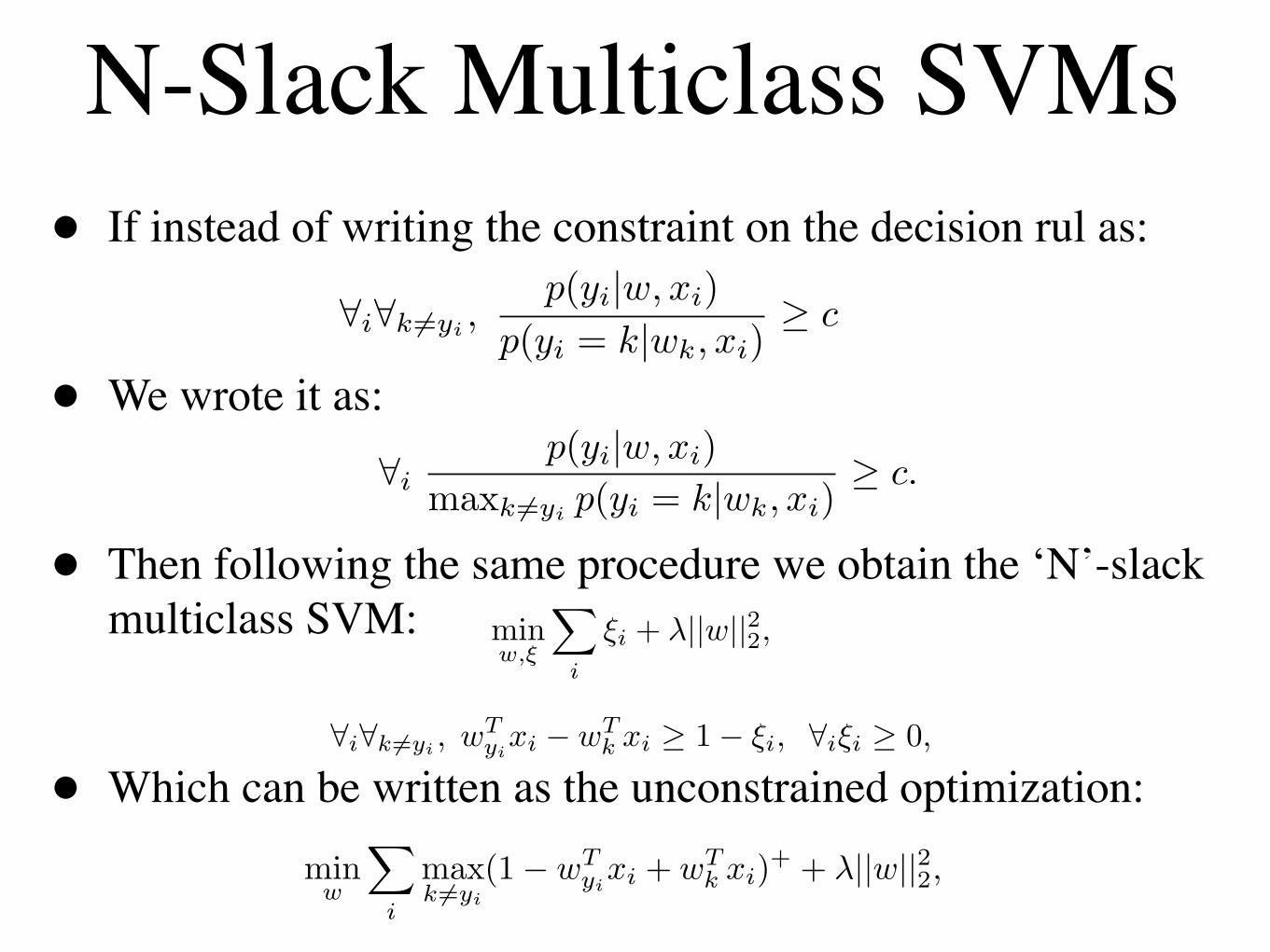
N-Slack Multiclass SVMs• If instead of writing the constraint on the decision rul as:

• We wrote it as:

• Then following the same procedure we obtain the ‘N’-slack multiclass SVM:

• Which can be written as the unconstrained optimization:



minw

∑

i

(1− yiwT xi)+ + λ||w||22,










yi = maxk

p(yi = k|wk, xi).









3


minw,ξ

∑

i

∑

k !=yi

ξi,k + λ||w||22,




minw

∑

i

∑

k !=yi

(1− wTyi

xi + wTk xi)+ + λ||w||22,



∀ip(yi|w, xi)



minw,ξ

∑

i

ξi + λ||w||22,




minw

∑

i

maxk !=yi

(1− wTyi

xi + wTk xi)+ + λ||w||22,






4


minw,ξ

∑

i

∑

k !=yi

ξi,k + λ||w||22,




minw

∑

i

∑

k !=yi

(1− wTyi

xi + wTk xi)+ + λ||w||22,



∀ip(yi|w, xi)



minw,ξ

∑

i

ξi + λ||w||22,




minw

∑

i

maxk !=yi

(1− wTyi

xi + wTk xi)+ + λ||w||22,






4


minw,ξ

∑

i

∑

k !=yi

ξi,k + λ||w||22,




minw

∑

i

∑

k !=yi

(1− wTyi

xi + wTk xi)+ + λ||w||22,



∀ip(yi|w, xi)



minw,ξ

∑

i

ξi + λ||w||22,




minw

∑

i

maxk !=yi

(1− wTyi

xi + wTk xi)+ + λ||w||22,






4


• Binary SVMs

• Multiclass SVMs

• Structural SVMs

• Training:

• Subgradients

• Cutting Planes



Conditional Random Fields• The extension of logistic regression to data with multiple

(dependent) labels is known as a conditional random field.

• For example, a binary chain-CRF with Ising-like potentials and tied parameters could use:

• A concise notation for the general case is:

• One possible decision rule is:

• In the case of chains, this is Viterbi decoding

label yi,j depends on the previous label yi,j−1. The structural extension of logistic regression to handle thistype of dependency structure is known as a linear-chain conditional random field [Lafferty et al., 2001]. Inthe case of tied parameters, binary labels, Ising-like potentials, and sequences of labels with the same lengthS (removing any of these restrictions is trivial, but would require more notation), the probability of a vectorof labels Yi is written as

p(Yi|w, Xi) ∝ exp(S∑

j=1

yi,jwTn xi,j +

S−1∑

j=1

yi,jyi,j+1wTe xi,j,j+1),

where wn represent the node parameters, we represent the edge/transition parameters, and we allow a featurevector xi,j for each node and xi,j,j+1 for each transition. Although there are other possibilities, we considerthe decision rule

Yi = maxYi

p(Yi|w, Xi).

Computing this maximum by considering all possible labels may no longer be feasible, since there are now2S possible labels, but the maximum can be found in O(S) by dynamic programming in the form of theViterbi decoding algorithm.

Moving to an interpretation in terms of likelihood ratios, we would like our classifier to satisfy the criteria

∀i∀Y ′i "=Yi

p(Yi|w, Xi)p(Y ′

i |w, Xi)≥ c,

leading to the set of constraints

∀i∀Y ′i "=Yi

log p(Yi|w, Xi)− log p(Y ′i |w, Xi) ≥ 1. (1)

Introducing the !2-norm (squared) regularizer and the N -slack constraint violation penalty, we obtain thequadratic program

minw,ξ

∑

i

ξi + λ||w||22,

s.t. ∀i∀Y ′i "=Yi

log p(Yi|w, Xi)− log p(Y ′i |w,Xi) ≥ 1− ξi, ∀i ξi ≥ 0

This is known as a hidden Markov support vector machine [Altun et al., 2003, Joachims, 2003].Because it is based on the N -slack formulation, the hidden Markov support vector machine penalizes all

alternative hypothesis based on the most promising alternative hypothesis. In particular, the number of labeldifferences between Yi and an alternative configuration Y ′

i is never considered. Rather than selecting theconstant to be 1 across all alternative configurations, we could consider setting it to ∆(Yi, Y ′

i ), the numberof label differences between Yi and Y ′

i

∀i∀Y ′i "=Yi

log p(Yi|w, Xi)− log p(Y ′i |w, Xi) ≥ ∆(Yi, Y

′i ). (2)

This encourages the likelihood ratio between the true label and an alternative configuration to be higherif the alternative configuration disagrees with Yi at many nodes. With our usual procedure we obtain thequadratic program

minw,ξ

∑

i

ξi + λ||w||22,


log p(Yi|w, Xi)− log p(Y ′i |w,Xi) ≥ ∆(Yi, Y

′i )− ξi, ∀iξi ≥ 0,

which is known as a max-margin Markov network [Taskar et al., 2003], or a structural support vector machinewith margin re-scaling [Tsochantaridis et al., 2004].

Of course, this isn’t the only way to change the constraints based on the agreement between Yi and Y ′i ,

and [Tsochantaridis et al., 2004] argues that this formulation has the disadvantage that it tries to make verylarge the difference between competing labels that differ in many positions. An alternative to changing the

5

the method requires O(1/ε) iterations to converge9, and that the method offers a speed advantage over themethod of [Shalev-Shwartz et al., 2007].

5.3 Polynomial-Size Reformulations

In this section, we examine an alternative to cutting plane methods for dealing with the exponential sizedquadratic programs. In particular, we consider methods that take advantage of the sparse dependency struc-ture in the underlying distribution to rewrite the exponential-sized quadratic program into a polynomial-sizedproblem. In this section, we will largely follow [Taskar et al., 2003] and will work with a dual formulationto the MMMN quadratic program. In this dual formulation, we will have a variable αi(Y ′

i ) for each possibleconfiguration Y ′

i of training example i. We will also find it convenient to use the feature representation ofthe probability functions

p(Yi|w,Xi) ∝ exp(wT F (Xi, Yi)),

and use the notation∆Fi(Y ′

i ) ! F (Xi, Yi)− F (Xi, Y′i ).

Using this notation, [Taskar et al., 2003] shows that the following problem is dual to the MMMN quadraticprogram

maxα

∑

i

∑

Y ′i

αi(Y ′i )∆(Yi, Y

′i )− 1

2

∑

i

∑

Y ′i

∑

j

∑

Y ′j

αi(Y ′i )αj(Y ′

j )∆Fi(Y ′i )T ∆Fj(Y ′

j ),

s.t. ∀i

∑

Y ′i

αi(Y ′i ) =

12λ

, ∀i∀Y ′iαi(Y ′

i ) ≥ 0.

Although this dual formulation has an exponential number of constraints and an exponential number ofvariables, note the simple form of the constraints. If λ = 1/2, then the constraints simply enforce thatαi(Y ′

i ) is a valid probability distribution over all values of Y ′i (for each training example i). For other

values of λ, it enforces that αi(Y ′i ) is an unnormalized distribution (with normalizing constant 1/2λ). If our

dependency structure factorizes over nodes and edges in a graph, then we can consider a parameterizationin terms of expectations with respect to this distribution

µi(yij) =∑

Y ′i ∼[yij ]

αi(Y ′i ),

µi(yij , yik) =∑

Y ′i ∼[yij ,yik]

αi(Y ′i ),

where the notation Y ′i ∼ [yij ] is used to denote that a configuration Y ′

i is consistent with the label yij . Whenwe consider using these variables, we will require that the node parameters satisfy the constraints of theoriginal problem

∀i∀j µi(yij) ≥ 0, ∀i

∑

j

µi(yij) =12λ

.

To ensure that the edge variables form a legal density, they must belong to the marginal polytope. In thecase of tree-structured graphs, this is equivalent to the requirement that [Taskar et al., 2003]

∀i∀(j,k)∈E

∑

yij

µi(yij , yik) = µi(yik), ∀i∀(j,k)∈E µi(yij , yik) ≥ 0.

Using these expectations, we can re-write the set of first terms in the dual formulation as∑

Y ′i


′i ) =

∑

Y ′i

∑

j

αi(Y ′i )∆j(yij , y

′ij) =

∑

j

∑

y′ij

∆j(yij , y′ij)µi(y′ij).

9[Smola et al., 2008] also show that applying their method to train conditional random fields with !2-regularization achievesthe faster rate of O(log(1/ε)).

10


p(Yi|w,Xi) ∝ exp(S∑

j=1

yi,jwTn xi,j +

S−1∑

j=1



Yi = maxYi

p(Yi|w,Xi).



∀i∀Y ′i "=Yi

p(Yi|w,Xi)p(Y ′

i |w,Xi)≥ c,


∀i∀Y ′i "=Yi

log p(Yi|w,Xi)− log p(Y ′i |w,Xi) ≥ 1. (1)


minw,ξ

∑

i

ξi + λ||w||22,


log p(Yi|w,Xi)− log p(Y ′i |w,Xi) ≥ 1− ξi, ∀i ξi ≥ 0





i

∀i∀Y ′i "=Yi

log p(Yi|w,Xi)− log p(Y ′i |w,Xi) ≥ ∆(Yi, Y

′i ). (2)


minw,ξ

∑

i

ξi + λ||w||22,



′i )− ξi, ∀iξi ≥ 0,




5

Hidden Markov SVMs• Making the right decisions with Viterbi decoding corresponds

to satisfying:

• This is equivalent to the set of constraints:

• Adding the L2-penalty and using the N-slack penalty:

• The ‘hidden Markov support vector machine’



j=1

yi,jwTn xi,j +

S−1∑

j=1



Yi = maxYi

p(Yi|w,Xi).



∀i∀Y ′i "=Yi

p(Yi|w,Xi)p(Y ′

i |w,Xi)≥ c,


∀i∀Y ′i "=Yi



minw,ξ

∑

i

ξi + λ||w||22,







i

∀i∀Y ′i "=Yi


′i ). (2)


minw,ξ

∑

i

ξi + λ||w||22,



′i )− ξi, ∀iξi ≥ 0,




5



j=1

yi,jwTn xi,j +

S−1∑

j=1



Yi = maxYi

p(Yi|w,Xi).



∀i∀Y ′i "=Yi

p(Yi|w,Xi)p(Y ′

i |w,Xi)≥ c,


∀i∀Y ′i "=Yi



minw,ξ

∑

i

ξi + λ||w||22,







i

∀i∀Y ′i "=Yi


′i ). (2)


minw,ξ

∑

i

ξi + λ||w||22,



′i )− ξi, ∀iξi ≥ 0,




5



j=1

yi,jwTn xi,j +

S−1∑

j=1



Yi = maxYi

p(Yi|w,Xi).



∀i∀Y ′i "=Yi

p(Yi|w,Xi)p(Y ′

i |w,Xi)≥ c,


∀i∀Y ′i "=Yi



minw,ξ

∑

i

ξi + λ||w||22,







i

∀i∀Y ′i "=Yi


′i ). (2)


minw,ξ

∑

i

ξi + λ||w||22,



′i )− ξi, ∀iξi ≥ 0,




5

Max-Margin Markov Networks• The constraints in the HMSVM don’t care about the number

of differences between Yi and Yi’:

• We might to be the difference in probability to be higher when the difference in labels is higher:

• Leading to the QP:

• This is known as a ‘max-margin Markov networks’, or ‘structural SVM’ with ‘margin-rescaling’



j=1

yi,jwTn xi,j +

S−1∑

j=1



Yi = maxYi

p(Yi|w,Xi).



∀i∀Y ′i "=Yi

p(Yi|w,Xi)p(Y ′

i |w,Xi)≥ c,


∀i∀Y ′i "=Yi



minw,ξ

∑

i

ξi + λ||w||22,







i

∀i∀Y ′i "=Yi


′i ). (2)


minw,ξ

∑

i

ξi + λ||w||22,



′i )− ξi, ∀iξi ≥ 0,




5



j=1

yi,jwTn xi,j +

S−1∑

j=1



Yi = maxYi

p(Yi|w,Xi).



∀i∀Y ′i "=Yi

p(Yi|w,Xi)p(Y ′

i |w,Xi)≥ c,


∀i∀Y ′i "=Yi



minw,ξ

∑

i

ξi + λ||w||22,







i

∀i∀Y ′i "=Yi


′i ). (2)


minw,ξ

∑

i

ξi + λ||w||22,



′i )− ξi, ∀iξi ≥ 0,




5



j=1

yi,jwTn xi,j +

S−1∑

j=1



Yi = maxYi

p(Yi|w,Xi).



∀i∀Y ′i "=Yi

p(Yi|w,Xi)p(Y ′

i |w,Xi)≥ c,


∀i∀Y ′i "=Yi



minw,ξ

∑

i

ξi + λ||w||22,







i

∀i∀Y ′i "=Yi


′i ). (2)


minw,ξ

∑

i

ξi + λ||w||22,



′i )− ξi, ∀iξi ≥ 0,




5

Structural SVMs• Rescaling the constant might make us concentrate on being

much better than sequences that differ at many positions:

• An alternative is to rescale the slacks based on the difference between sequences:

• Leading to the QP:

• This is known as a ‘structural SVM’ with ‘slack-rescaling’



j=1

yi,jwTn xi,j +

S−1∑

j=1



Yi = maxYi

p(Yi|w,Xi).



∀i∀Y ′i "=Yi

p(Yi|w,Xi)p(Y ′

i |w,Xi)≥ c,


∀i∀Y ′i "=Yi



minw,ξ

∑

i

ξi + λ||w||22,







i

∀i∀Y ′i "=Yi


′i ). (2)


minw,ξ

∑

i

ξi + λ||w||22,



′i )− ξi, ∀iξi ≥ 0,




5

constant factor in the likelihood ratio is to change the scaling of the slack variables and solve the quadraticprogram

minw,ξ

∑

i

ξi + λ||w||22,

s.t. ∀i∀Y ′i !=Yi

log p(Yi|w,Xi)− log p(Y ′i |w,Xi) ≥ 1− ξi/∆(Yi, Y

′i ), ∀iξi ≥ 0.

Here, you need to add more ‘slack’ for a competing hypothesis that differs in many position. This last variantis known as a structural support vector machine with slack re-scaling [Tsochantaridis et al., 2004].

Equivalent unconstrained versions of these 3 structural extensions of support vector machines are3

(HMSVM) minw

∑

i

maxY ′

i !=Yi

(1− log p(Yi|w,Xi) + log p(Y ′i |w,Xi))+ + λ||w||22,

(MMMN) minw

∑

i

maxY ′

i !=Yi

(∆(Yi, Y′i )− log p(Yi|w,Xi) + log p(Y ′

i |w,Xi))+ + λ||w||22,

(SSVM) minw

∑

i

maxY ′

i !=Yi

(∆(Yi, Y′i )(1− log p(Yi|w,Xi) + log p(Y ′

i |w,Xi)))+ + λ||w||22.

In the (MMMN) and (SSVM) formulations, we can use ∆(Yi, Yi) = 0 to simplify these expressions, giving

(MMMN) minw

∑

i

maxY ′

i

(∆(Yi, Y′i ) + log p(Y ′

i |w,Xi))− log p(Yi|w,Xi) + λ||w||22,

(SSVM) minw

∑

i

maxY ′

i


i |w,Xi))) + λ||w||22.

N.B., in these latter two expressions we can maximize over all Y ′i instead of over all Y ′

i $= Yi; In these cases,we can compute the objective function using the Viterbi decoding algorithm (with a suitably modified input).In contrast, the HMSVM model requires solving a maximization problem over all configurations except Yi,which be may be much harder to solve4. Finally, we note that while the structural hinge losses in all threeformulations represent an upper bound on the number of sequence errors (ie. the number of times at leastone label in the sequence was wrong), the MMMN and SSVM formulations give an upper bound on thenumber of label errors while the HMSVM does not.

Although this section has focused on a chain-structured dependency structure, we only used this propertyin two places: (i) the definition of p(Yi|w,Xi), and (ii) in efficient methods to compute maximums over thespace of possible configurations. We can apply the same methodology to derive MMMNs and SSVMs fora wide variety of alternative models. For example, we can consider the cases where conditional randomfields can be applied exactly, such as low tree-width structured dependencies, and probabilistic context freegrammars. We can also consider models where we consider higher-order dependencies, rather than simplypairwise dependencies, as long as the graph structure or parameterization allows us to efficiently solve theassociated maximization problems.

As discussed in [Taskar et al., 2004], an advantage that MMMNs/SSVMs have over conditional randomfields is that we can also consider completely general graph structures (such as lattices or fully connectedgraphs), if we enforce the additional constraint that the edge weights enforce a sub-modularity condition[Kolmogorov and Zabin, 2004]. In these cases, the exact inference needed for training conditional randomfields is intractable, but computing the maximums needed by MMMNs/SSVMs can be formulated as a linearprogram (that can be efficiently solved using min-cut techniques). [Taskar et al., 2004] proposes associativemax margin Markov networks, models that take advantage of this property to allow efficient training anddecoding in models with an arbitrary graph structure and arbitrary clique sizes. In these models, the

3We can also consider penalizing the squared values of the slack variables [Tsochantaridis et al., 2004], but this does notlead to a differentiable minimization problem due to the potential for ties in the max functions.

4We could also consider structural extensions based on the NK-slack formulation [Altun and Hofmann, 2003]. In this case,the max functions would be replaced by sums, but it is not obvious (to me, anyway) how you would compute these sumsefficiently, nor how you would deal with the exponential number of variables and constraints in the quadratic program

6


minw,ξ

∑

i

ξi + λ||w||22,



′i ), ∀iξi ≥ 0.



(HMSVM) minw

∑

i

maxY ′

i !=Yi


(MMMN) minw

∑

i

maxY ′

i !=Yi


i |w,Xi))+ + λ||w||22,

(SSVM) minw

∑

i

maxY ′

i !=Yi


i |w,Xi)))+ + λ||w||22.


(MMMN) minw

∑

i

maxY ′

i

(∆(Yi, Y′i ) + log p(Y ′


(SSVM) minw

∑

i

maxY ′

i


i |w,Xi))) + λ||w||22.







6

Summary• Unconstrained formulations of structural extensions:

• Since delta(Yi,Yi)=0, we simplify MMMN and SSVM:

• This allows us to use Viterbi decoding with a modified input to compute the max values.


minw,ξ

∑

i

ξi + λ||w||22,



′i ), ∀iξi ≥ 0.



(HMSVM) minw

∑

i

maxY ′

i !=Yi


(MMMN) minw

∑

i

maxY ′

i !=Yi


i |w,Xi))+ + λ||w||22,

(SSVM) minw

∑

i

maxY ′

i !=Yi


i |w,Xi)))+ + λ||w||22.


(MMMN) minw

∑

i

maxY ′

i

(∆(Yi, Y′i ) + log p(Y ′


(SSVM) minw

∑

i

maxY ′

i


i |w,Xi))) + λ||w||22.







6


minw,ξ

∑

i

ξi + λ||w||22,



′i ), ∀iξi ≥ 0.



(HMSVM) minw

∑

i

maxY ′

i !=Yi


(MMMN) minw

∑

i

maxY ′

i !=Yi


i |w,Xi))+ + λ||w||22,

(SSVM) minw

∑

i

maxY ′

i !=Yi


i |w,Xi)))+ + λ||w||22.


(MMMN) minw

∑

i

maxY ′

i

(∆(Yi, Y′i ) + log p(Y ′


(SSVM) minw

∑

i

maxY ′

i


i |w,Xi))) + λ||w||22.







6

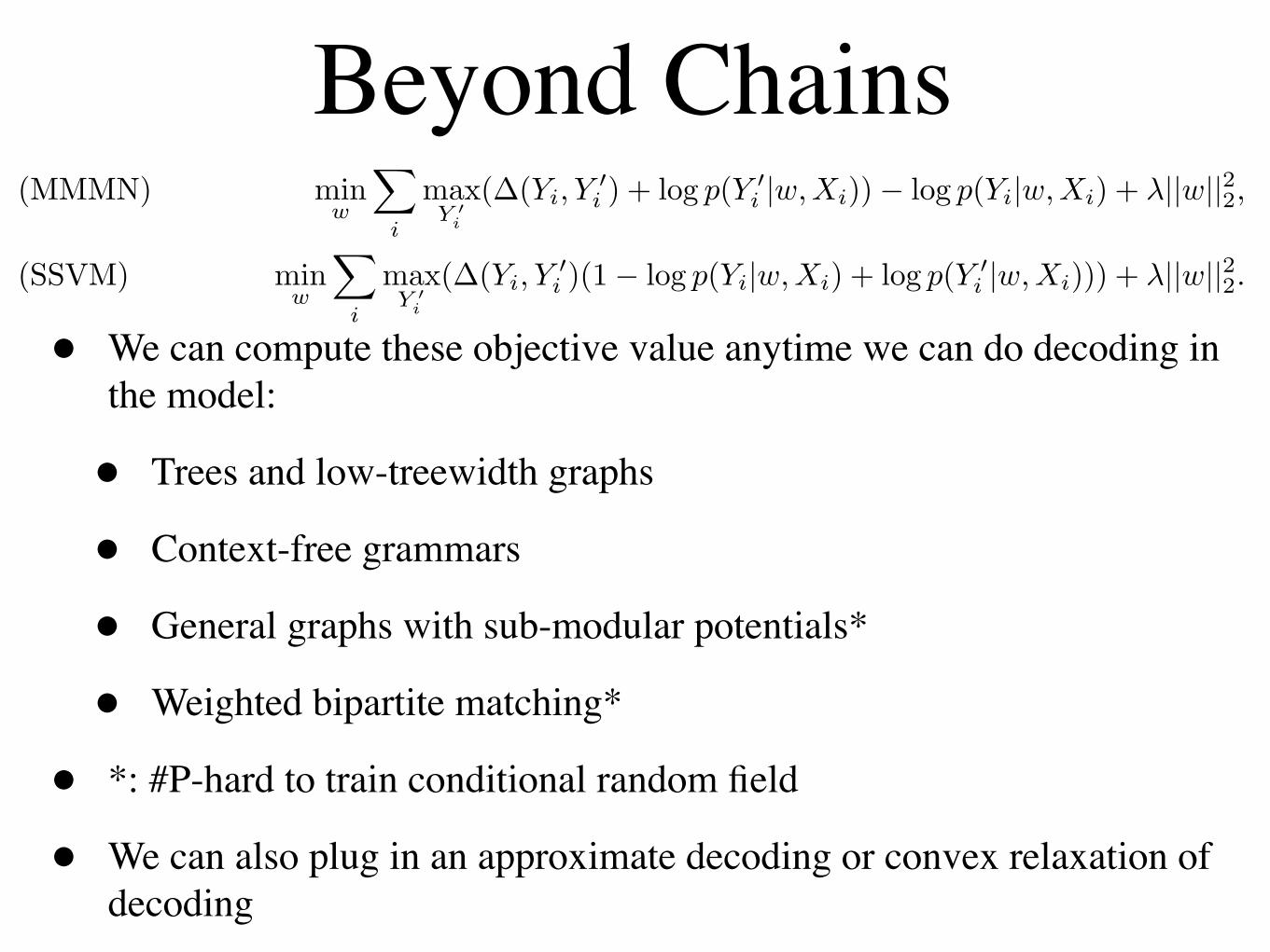
Beyond Chains

• We can compute these objective value anytime we can do decoding in the model:

• Trees and low-treewidth graphs

• Context-free grammars

• General graphs with sub-modular potentials*

• Weighted bipartite matching*

• *: #P-hard to train conditional random field

• We can also plug in an approximate decoding or convex relaxation of decoding


minw,ξ

∑

i

ξi + λ||w||22,



′i ), ∀iξi ≥ 0.



(HMSVM) minw

∑

i

maxY ′

i !=Yi


(MMMN) minw

∑

i

maxY ′

i !=Yi


i |w,Xi))+ + λ||w||22,

(SSVM) minw

∑

i

maxY ′

i !=Yi


i |w,Xi)))+ + λ||w||22.


(MMMN) minw

∑

i

maxY ′

i

(∆(Yi, Y′i ) + log p(Y ′


(SSVM) minw

∑

i

maxY ′

i


i |w,Xi))) + λ||w||22.







6


• Binary SVMs

• Multiclass SVMs

• Structural SVMs

• Training:

• Subgradients

• Cutting Planes



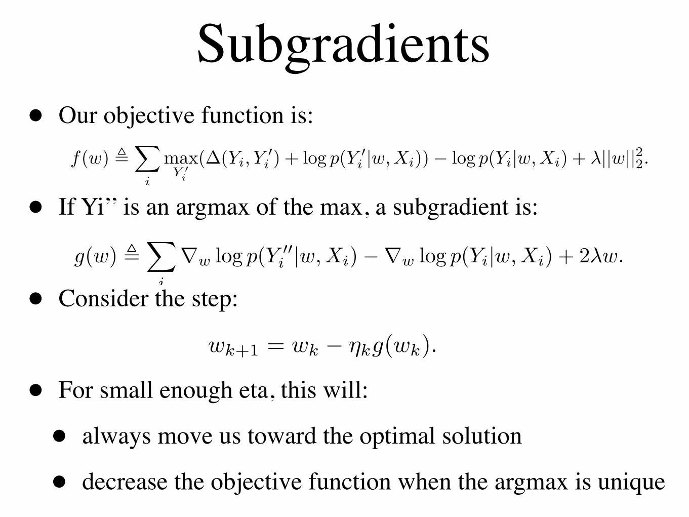
Subgradients• Our objective function is:

• If Yi’’ is an argmax of the max, a subgradient is:

• Consider the step:

• For small enough eta, this will:

• always move us toward the optimal solution

• decrease the objective function when the argmax is unique

potential that all variables in a clique take the state k based on a non-negative feature xi is modeled with aparameter λk,i ≥ 1, while the potential for any configuration where they don’t take the same state is fixedat 1. For binary variables, the decoding problem can be solved exactly as a linear program for any graphstructure, while for multi-class problems the linear program yields a worst-case approximation ratio of 1/c(where c is the largest clique size), if an appropriate discretization strategy is used. [Taskar et al., 2006b]also gives the example of weighted bipartite graph matching, where decoding can be computed in polynomialtime using linear programming, but the inference needed to train a conditional random field is #P -hard.

For general graphs where we do not want the sub-modularity condition, we can also consider an approxi-mation where we use an approximate decoding method, such as loopy belief propagation or a stochastic localsearch method [Hutter et al., 2005]). However, theoretical and empirical work in [Finley and Joachims, 2008]shows that using such under-generating decoding methods (which may return sub-optimal solutions to thedecoding problem) have several disadvantages compared to so-called over-generating decoding methods. Atypical example of an over-generating decoding method is a linear programming relaxation of an integerprogramming formulations of decoding, where in the relaxation the objective is optimized exactly over anexpanded space [Kumar et al., 2007], hence yielding a fractional decoding that is a strict upper bound onthe optimal decoding.

5 Training

In this section, we discuss methods for estimating the parameters of structural extensions of SVMs. We willfocus on MMMNs since it makes the notation slightly simpler, but most of the techniques can be appliedwith only minor modifications to the case of SSVMs.

5.1 Subgradient Methods

We first consider methods that address the unconstrained non-differentiable formulation of MMMNs bymoving along sub-gradients of the objective function

f(w) !∑

i

maxY ′

i

(∆(Yi, Y′i ) + log p(Y ′

i |w,Xi))− log p(Yi|w,Xi) + λ||w||22.

If we use Y ′′i as an argmax of the max, then a sub-gradient of this objective function is

g(w) !∑

i

∇w log p(Y ′′i |w,Xi)−∇w log p(Yi|w,Xi) + 2λw.

The function is differentiable and this will be the gradient whenever all of the argmax values are unique.The negative sub-gradient direction is a descent direction at all points where the function is differentiable,which means that f(w− ηg(w)) < f(w) for sufficiently small η > 0. In contrast, at non-differentiable points(where at least one argmax is not unique) negative sub-gradient directions may not be descent directions[Bertsekas, 1999, §6.3]. However, we can guarantee that for sufficiently small η the distance to the optimalsolution is reduced, even if the function value is not [Bertsekas, 1999, §6.3]. We can therefore consider asimple sub-gradient method that uses a sequence of small step sizes {ηk}, where the iterations take of theform

wk+1 = wk − ηkg(wk).

Several strategies for choosing the step length that lead to convergence of the iterations are discussed in[Bertsekas, 1999, §6.3], with a common choice being a sequence {ηk} of positive step sizes satisfying

∞∑

k=1

ηk =∞,∞∑

k=1

η2k <∞.

7



5 Training




f(w) !∑

i

maxY ′

i

(∆(Yi, Y′i ) + log p(Y ′



g(w) !∑

i





∞∑

k=1

ηk =∞,∞∑

k=1

η2k <∞.

7



5 Training




f(w) !∑

i

maxY ′

i

(∆(Yi, Y′i ) + log p(Y ′



g(w) !∑

i





∞∑

k=1

ηk =∞,∞∑

k=1

η2k <∞.

7

Subgradient descent• We can therefore consider optimization algorithms of the form:

• Common choices of step size are constant, or a sequence satisfying:

• Update based on a single training example:

• Average the iterations:

• Project onto a compact set containing the solution:



5 Training




f(w) !∑

i

maxY ′

i

(∆(Yi, Y′i ) + log p(Y ′



g(w) !∑

i





∞∑

k=1

ηk =∞,∞∑

k=1

η2k <∞.

7



5 Training




f(w) !∑

i

maxY ′

i

(∆(Yi, Y′i ) + log p(Y ′



g(w) !∑

i





∞∑

k=1

ηk =∞,∞∑

k=1

η2k <∞.

7

Convergence of the method can also be shown if each step uses the contribution to the sub-gradient of asuitably chosen individual training example i [Kushner and Yin, 2003]

gi(w) ! ∇w log p(Y ′′i |w,Xi)−∇w log p(Yi|w,Xi) + (2/N)λw,

resulting in steps of the formwk+1 = wk − ηkgi(wk).

This is known as a stochastic sub-gradient descent method, and was presented in [Collins, 2002] (predatingthe formulation of structural SVMs) for the degenerate case of λ = 0 and ∀Yi,Y ′

i∆(Yi, Y ′

i ) = 0, and where aconstant step size (ηk = η) was used instead of a convergent sequence.

An interesting alternative method was also outlined in [Collins, 2002]; In this second method a constantstep size was used, and a variant on the procedure was considered where the final estimator is the averageof all the iterates;

wk+1 = wk − ηgi(wk),

wk+1 =k − 1

kwk +

1k

wk+1.

Convergence of averaged estimators of the form w is discussed in [Kushner and Yin, 2003], where it is shownthat under certain conditions these steps satisfy an asymptotic statistical efficiency property.

In the special case of binary support vector machines (though easily extended to structural support vectormachines), [Shalev-Shwartz et al., 2007] considers iterations of the form

wk+1 = π(wk − ηkg(wk)),

where π is a projection onto an $2-ball that is guaranteed to contain the solution5. They showed that the num-ber of iterations to obtain a solution with accuracy ε using this method is O(1/ε) (ignoring poly-logarithmicfactors), which was an improvement over the O(1/ε2) number of iterations provided by the previous anal-ysis of the averaged stochastic gradient method [Zhang, 2004] and cutting plane methods [Joachims, 2006].[Shalev-Shwartz et al., 2007] also consider the case of a projected stochastic gradient update, and showthat the iterations achieve an accuracy of ε with probability 1 − δ in O(1/(δε)) iterations. One couldalso consider combining averaging and projections, whose asymptotic statistical efficiency is considered in[Kushner and Yin, 2003]. Finally, [Ratliff et al., 2007] show that the (deterministic) subgradient methodwith a sufficiently small constant step size will converge linearly (ie. with the faster rate of O(log(1/ε)))to a region containing the minimum whose radius is proportional to C/λ (where C is a bound on thesub-differential).

5.2 Cutting Plane and Bundle Methods

We now consider methods for solving the quadratic programming formulation of MMMNs

minw,ξ

∑

i

ξi + λ||w||22,

s.t. ∀i∀Y ′ilog p(Yi|w,Xi)− log p(Y ′

i |w,Xi) ≥ ∆(Yi, Y′i )− ξi, ∀iξi ≥ 0.

This formulation is problematic since we have an exponential number of constraints. However, it is con-ceivable that we do not need to enforce all of these constraints at the optimal solution. In particular,[Tsochantaridis et al., 2004] showed that there always exists a polynomial-sized subset of the constraintsthat can satisfy all constraints with accuracy at least ε. This makes cutting-plane methods for quadraticprogramming an appealing approach for solving this type of problem.

Cutting plane methods have a very simple structure; We first find the unconstrained minimizer. If theminimizer does not satisfy all the constraints, we find a constraint that is violated and use it to construct our

5The projection of a vector w onto a set W is defined as minw∗∈W ||w − w∗||2

8





i∆(Yi, Y ′




wk+1 =k − 1

kwk +

1k

wk+1.







minw,ξ

∑

i

ξi + λ||w||22,


i |w,Xi) ≥ ∆(Yi, Y′i )− ξi, ∀iξi ≥ 0.




8





i∆(Yi, Y ′




wk+1 =k − 1

kwk +

1k

wk+1.







minw,ξ

∑

i

ξi + λ||w||22,


i |w,Xi) ≥ ∆(Yi, Y′i )− ξi, ∀iξi ≥ 0.




8

Some Convergence Rates• Projected batch SD (diminishing step sizes): O(1/eps)

• Averaged stochastic SD (constant step sizes): O(1/eps2), asymptotic variance

• Stochastic projected SD (dimishing step sizes): O(1/(d eps)) w.p. 1-d

• Averaged stochastic projected SD (constant step sizes): ?, asymptotic variance

• Batch SD (constant step sizes): O(log(1/eps)) to get within bounded region of optimal (bound depends on lambda and bound on sub-differential)


• Binary SVMs

• Multiclass SVMs

• Structural SVMs

• Training:

• Subgradients

• Cutting Planes



Cutting Plane Methods• The problem with the QP formulation is that it has an exponential

number of constraints:

• But, there always exists a polynomial-sized set that satisfies all constraints up to an accuracy of eps.

• Basic idea behind cutting plane method:

• use decoding to find out if all constraints are satisfied

• if not, greedily add a constraint





i∆(Yi, Y ′




wk+1 =k − 1

kwk +

1k

wk+1.







minw,ξ

∑

i

ξi + λ||w||22,


i |w,Xi) ≥ ∆(Yi, Y′i )− ξi, ∀iξi ≥ 0.




8

QP Cutting Plane Method• Cutting plane method:

• we have a working set of constraints

• iterate over training examples:

• if decoding does not violate constraints, continue

• otherwise, add constraint to working set and solve QP

• stop if no changes in working set

• Solving these QPs in the dual is efficient, as long as the working set is small.

• At most O(1/eps) constraints are required.

Convex Cutting Plane• There also exist ‘cutting plane’ methods for solving (non-

smooth) convex optimization problems

• We can apply these to the unconstrained formulation:

• Basic idea: any subgradient gives a lower bounding hyper-plane

• Cutting plane for non-smooth optimization:

• Find minimum over these lower bounds

• Use minimum to make better lower bound



5 Training




f(w) !∑

i

maxY ′

i

(∆(Yi, Y′i ) + log p(Y ′



g(w) !∑

i





∞∑

k=1

ηk =∞,∞∑

k=1

η2k <∞.

7

initial working set W. We then solve the problem with the constraints contained in W, and if this solutionstill does not satisfy all the constraints we add another violating constraint to W. This continues until wehave accumulated enough constraints in W so that all constraints are satisfied in the solution.

[Tsochantaridis et al., 2004] suggests the following implementation of a cutting plane algorithm for MMMNs.We iterate over the training examples, and use Viterbi decoding to find the maximum structural hinge loss.If no constraint is violated by more than ε then we move on to the next training example. Otherwise, we addthe constraint corresponding to this alternative configuration, and optimize the objective function subjectto our current working set of constraints. The algorithm terminates when we complete a full pass throughthe training data without adding any constraints.

The quadratic programs can be efficiently solved using the Wolfe dual formulation (see the next section),which is a relatively small problem since it has only one variable for each working constraint. Further, thesequence of quadratic programs can be solve efficiently since each quadratic program differs from the previousone by only a single constraint. The main concern with using this type of approach is that the number ofconstraints needed might be so large that the intermediate quadratic programs may be impractical to solve.[Tsochantaridis et al., 2004] show that at most O(1/ε2) constraints are required6.

This cutting plane algorithm for structural SVMs later inspired an efficient algorithm for binary supportvector machines [Joachims, 2006]. In this method, the binary support vector machine problem is written ina so-called 1-slack formulation

minw,ξ

Nξ + λ||w||22,

s.t. ∀c∈{0,1}N

∑

i

ciyiwT xi ≥

∑

i

ci −Nξ, ξ ≥ 0.

Here, we have an exponential number of constraints but only 1 slack variable. [Joachims, 2006] shows thatthis formulation has the same optimal parameters (with ξ = (1/N)

∑i ξi), and outlines a cutting plane

algorithm for binary SVMs that is implemented in the SVMperf software7. This method was extended(back) to structural SVMs in [Joachims et al., 2009], where it was shown that at most O(1/ε) constraintsare required. This is the algorithm implemented in the current version of the SVMstruct software8.

An alternative to applying cutting plane methods for quadratic programming to a constrained formulationof the MMMN problem is to apply the related cutting plane methods for non-smooth optimization to theunconstrained non-differentiable MMMN problem. This is explored in [Teo et al., 2007, Smola et al., 2008].

In cutting plane methods for optimization of (non-smooth) convex functions, we use the definition of asub-gradient at a point w0 to yield a global lower bound on the function

f(w) ≥ f(w0) + (w − w0)T g(w0),

that is exact at w0. Cutting plane methods for non-smooth optimization proceed by collecting a set ofthese lower bounding hyper-planes, and at each iteration generate a new trial point by finding the minimumof these lower bounds. The function value and sub-gradient at the new trial point are then added to theworking set, yielding a more accurate lower bound.

A disadvantage of this procedure is that the minimum of the set of lower bounds may suggest a trialpoint that is far away from the previous point, even if the previous point was close to the optimal solution.This is known as instability [Bertsekas, 1999, §6.3]. A common way to address this is to minimize the lowerbound subject to a regularizer ||wk+1 − wk||22 on the difference between subsequent trial values. This isknown as a bundle method. The method of [Teo et al., 2007, Smola et al., 2008] is closely related to bundlemethods, but differs in the regularizer. Rather than building a lower bound for the full objective functionand using the regularizer ||wk+1−wk||22, they build a sequence of lower bounds for the hinge loss and use theexact regularizer λ||w||22 already present in the objective function. In [Smola et al., 2008], it is shown that

6A closely related method and analysis for HMSVMs is in [Joachims, 2003]7http://svmlight.joachims.org/svm perf.html8http://svmlight.joachims.org/svm struct.html

9

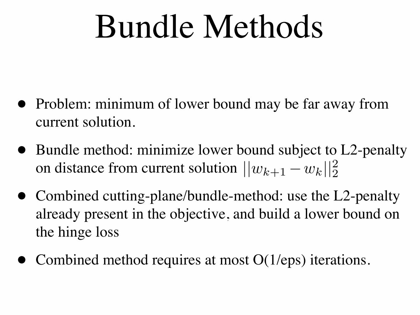
Bundle Methods

• Problem: minimum of lower bound may be far away from current solution.

• Bundle method: minimize lower bound subject to L2-penalty on distance from current solution

• Combined cutting-plane/bundle-method: use the L2-penalty already present in the objective, and build a lower bound on the hinge loss

• Combined method requires at most O(1/eps) iterations.

initial working set W. We then solve the problem with the constraints contained in W, and if this solutionstill does not satisfy all the constraints we add another violating constraint to W. This continues until wehave accumulated enough constraints in W so that all constraints are satisfied in the solution.

[Tsochantaridis et al., 2004] suggests the following implementation of a cutting plane algorithm for MMMNs.We iterate over the training examples, and use Viterbi decoding to find the maximum structural hinge loss.If no constraint is violated by more than ε then we move on to the next training example. Otherwise, we addthe constraint corresponding to this alternative configuration, and optimize the objective function subjectto our current working set of constraints. The algorithm terminates when we complete a full pass throughthe training data without adding any constraints.

The quadratic programs can be efficiently solved using the Wolfe dual formulation (see the next section),which is a relatively small problem since it has only one variable for each working constraint. Further, thesequence of quadratic programs can be solve efficiently since each quadratic program differs from the previousone by only a single constraint. The main concern with using this type of approach is that the number ofconstraints needed might be so large that the intermediate quadratic programs may be impractical to solve.[Tsochantaridis et al., 2004] show that at most O(1/ε2) constraints are required6.

This cutting plane algorithm for structural SVMs later inspired an efficient algorithm for binary supportvector machines [Joachims, 2006]. In this method, the binary support vector machine problem is written ina so-called 1-slack formulation

minw,ξ

Nξ + λ||w||22,

s.t. ∀c∈{0,1}N

∑

i

ciyiwT xi ≥

∑

i

ci −Nξ, ξ ≥ 0.

Here, we have an exponential number of constraints but only 1 slack variable. [Joachims, 2006] shows thatthis formulation has the same optimal parameters (with ξ = (1/N)

∑i ξi), and outlines a cutting plane

algorithm for binary SVMs that is implemented in the SVMperf software7. This method was extended(back) to structural SVMs in [Joachims et al., 2009], where it was shown that at most O(1/ε) constraintsare required. This is the algorithm implemented in the current version of the SVMstruct software8.

An alternative to applying cutting plane methods for quadratic programming to a constrained formulationof the MMMN problem is to apply the related cutting plane methods for non-smooth optimization to theunconstrained non-differentiable MMMN problem. This is explored in [Teo et al., 2007, Smola et al., 2008].

In cutting plane methods for optimization of (non-smooth) convex functions, we use the definition of asub-gradient at a point w0 to yield a global lower bound on the function

f(w) ≥ f(w0) + (w − w0)T g(w0),

that is exact at w0. Cutting plane methods for non-smooth optimization proceed by collecting a set ofthese lower bounding hyper-planes, and at each iteration generate a new trial point by finding the minimumof these lower bounds. The function value and sub-gradient at the new trial point are then added to theworking set, yielding a more accurate lower bound.

A disadvantage of this procedure is that the minimum of the set of lower bounds may suggest a trialpoint that is far away from the previous point, even if the previous point was close to the optimal solution.This is known as instability [Bertsekas, 1999, §6.3]. A common way to address this is to minimize the lowerbound subject to a regularizer ||wk+1 − wk||22 on the difference between subsequent trial values. This isknown as a bundle method. The method of [Teo et al., 2007, Smola et al., 2008] is closely related to bundlemethods, but differs in the regularizer. Rather than building a lower bound for the full objective functionand using the regularizer ||wk+1−wk||22, they build a sequence of lower bounds for the hinge loss and use theexact regularizer λ||w||22 already present in the objective function. In [Smola et al., 2008], it is shown that

6A closely related method and analysis for HMSVMs is in [Joachims, 2003]7http://svmlight.joachims.org/svm perf.html8http://svmlight.joachims.org/svm struct.html

9


• Binary SVMs

• Multiclass SVMs

• Structural SVMs

• Training:

• Subgradients

• Cutting Planes



Poly-sized Formulations

• The previous two strategies use the graph structure to allow efficient decoding.

• An alternative strategy is to use the graph structure to re-parameterize our quadratic program.

• Although we can also do this for the primal, this can be shown more directly for the dual problem...

Dual MMMN• Solving the MMMN QP is equivalent to solving the

following QP:

• Notes:

• this QP has an exponential number of constraints/variables

• the constraints take the form of an unnormalized distribution over label configurations

• We are going to write this QP in terms of marginals of this distribution








i ) ! F (Xi, Yi)− F (Xi, Y′i ).


maxα

∑

i

∑

Y ′i


′i )− 1

2

∑

i

∑

Y ′i

∑

j

∑

Y ′j



j ),

s.t. ∀i

∑

Y ′i

αi(Y ′i ) =

12λ


i ) ≥ 0.





µi(yij) =∑

Y ′i ∼[yij ]

αi(Y ′i ),

µi(yij , yik) =∑


αi(Y ′i ),




∑

j

µi(yij) =12λ

.


∀i∀(j,k)∈E

∑

yij



Y ′i


′i ) =

∑

Y ′i

∑

j


′ij) =

∑

j

∑

y′ij



10

Marginal Representation• If the distribution factorizes into node and edge potentials,

we can write the marginals of the distribution as:

• We must satisfy the constraints of the original problem:

• We also need the node and edge marginals to lie in the ‘marginal polytope’. For chains/trees/forests, it is sufficient to enforce a local consistency condition:








i ) ! F (Xi, Yi)− F (Xi, Y′i ).


maxα

∑

i

∑

Y ′i


′i )− 1

2

∑

i

∑

Y ′i

∑

j

∑

Y ′j



j ),

s.t. ∀i

∑

Y ′i

αi(Y ′i ) =

12λ


i ) ≥ 0.





µi(yij) =∑

Y ′i ∼[yij ]

αi(Y ′i ),

µi(yij , yik) =∑


αi(Y ′i ),




∑

j

µi(yij) =12λ

.


∀i∀(j,k)∈E

∑

yij



Y ′i


′i ) =

∑

Y ′i

∑

j


′ij) =

∑

j

∑

y′ij



10








i ) ! F (Xi, Yi)− F (Xi, Y′i ).


maxα

∑

i

∑

Y ′i


′i )− 1

2

∑

i

∑

Y ′i

∑

j

∑

Y ′j



j ),

s.t. ∀i

∑

Y ′i

αi(Y ′i ) =

12λ


i ) ≥ 0.





µi(yij) =∑

Y ′i ∼[yij ]

αi(Y ′i ),

µi(yij , yik) =∑


αi(Y ′i ),




∑

j

µi(yij) =12λ

.


∀i∀(j,k)∈E

∑

yij



Y ′i


′i ) =

∑

Y ′i

∑

j


′ij) =

∑

j

∑

y′ij



10








i ) ! F (Xi, Yi)− F (Xi, Y′i ).


maxα

∑

i

∑

Y ′i


′i )− 1

2

∑

i

∑

Y ′i

∑

j

∑

Y ′j



j ),

s.t. ∀i

∑

Y ′i

αi(Y ′i ) =

12λ


i ) ≥ 0.





µi(yij) =∑

Y ′i ∼[yij ]

αi(Y ′i ),

µi(yij , yik) =∑


αi(Y ′i ),




∑

j

µi(yij) =12λ

.


∀i∀(j,k)∈E

∑

yij



Y ′i


′i ) =

∑

Y ′i

∑

j


′ij) =

∑

j

∑

y′ij



10

Polynomial-Sized Dual• We can re-write the first set of terms in the dual using these

marginals:

• We can similarly write the second set of terms, yielding a polynomial-sized version of the dual problem:

• ‘Structural SMO’; coordinate descent on this problem








i ) ! F (Xi, Yi)− F (Xi, Y′i ).


maxα

∑

i

∑

Y ′i


′i )− 1

2

∑

i

∑

Y ′i

∑

j

∑

Y ′j



j ),

s.t. ∀i

∑

Y ′i

αi(Y ′i ) =

12λ


i ) ≥ 0.





µi(yij) =∑

Y ′i ∼[yij ]

αi(Y ′i ),

µi(yij , yik) =∑


αi(Y ′i ),




∑

j

µi(yij) =12λ

.


∀i∀(j,k)∈E

∑

yij



Y ′i


′i ) =

∑

Y ′i

∑

j


′ij) =

∑

j

∑

y′ij



10

This is now a sum over individual label assignments rather than over joint assignments. We can similarlyre-write the second term in the dual in terms of edge expectations. This leads to what [Taskar et al., 2003]calls the factored dual

maxµ

∑

i

∑

j

∑

y′ij

∆j(yij , y′ij)µi(y′ij)−

12

∑

i

∑

i′

∑

(j,k)∈E

∑

(j′,k′)∈E

∑

y′ij ,y′

ik

∑

y′i′j′ ,y

′i′k′

µi(y′ij , y′ik)µi′(y′i′j′ , y′i′k′)Fi(Xi, y

′ij , y

′ik)T Fi(Xi, y

′i′j′ , y′i′k′),

s.t. ∀i∀j µi(yij) ≥ 0, ∀i

∑

j

µi(yij) =12λ

,

∀i∀(j,k)∈E

∑

yij


While this formulation is now polynomial-size, the quadratic form has a very large number of terms (ie. itis quadratic in the number of training examples and instances). [Taskar et al., 2003] proposes a method,known as the structural SMO method, for solving this optimization problem. In this method, violation ofthe constrained optimality conditions is used to select the two most violating variables, and their optimalvalue given all the other variables is computed in closed form to update the variables.

[Taskar et al., 2003] discusses extensions of the above method to graph structures that are not forests.For triangulated graphs, additional constraints can be imposed to ensure that the distribution remains inthe marginal polytope, although the number of additional constraints is exponential in the worst case. If wehave an untriangulated graph or do not want to triangulate and add these extra constraints, the factoreddual can be solved as an approximation (analogous to loopy belief propagation). It is also possible to derivefactored duals when the original distribution factorizes over higher-order cliques. Finally, [Taskar et al., 2003]discusses a factored version of the primal problem, where we have an extended set of slack variables thatmimic the dependency structure in the graph and constrain dual variables enforcing constraints on themarginal polytope.

An alternative method for optimizing the dual formulation using a polynomial-sized number of variables isoutlined in [Bartlett et al., 2005, Collins et al., 2008]. In this method, the exponentiated gradient algorithmis used to (indirectly) optimize the variables α in the dual formulation. The exponentiated gradient algorithm[Kivinen and Warmuth, 1997] is a method to optimize a function f(x), where x lies on the probabilitysimplex10

∀ixi ≥ 0,∑

i

xi = 1.

The exponentiated gradient algorithm takes steps of the form

xi =xi exp(−η∇if(x))∑i′ xi′ exp(−η∇i′f(x))

,

where as before η is a learning rate, and we can consider applying the algorithm using the contribution tothe gradient of one training example at a time instead of all the training examples at once.

[Bartlett et al., 2005, Collins et al., 2008] work with a slightly modified dual formulation where the con-straints take the form of a probability simplex (instead of an unnormalized version), and apply the exponen-tiated gradient algorithm to this problem. To avoid dealing with the exponential number of variables α, theyuse an implicit representation for α in terms of variables that are analogous to the µ variables above. Similarto the methods from previous sections, they show that the method requires O(1/ε) iterations to reach anaccuracy of ε, and that this applies whether the full gradient or the gradient contribution from an individual

10[Kivinen and Warmuth, 1997] also outline an extension that can handle non-negative variables subject to the !1-norm ofthe vector being 1, and extensions where the constant 1 is replaced by another known constant C.

11

Exponentiated Gradient

• An alternative to using an explicity formulation of the dual is to use an implicit formulation apply the exponentiated gradient (EG) algorithm.

• The EG algorithm solves optimization problem where the variables take the form of a distribution:

• EG steps take the form:


maxµ

∑

i

∑

j

∑

y′ij


12

∑

i

∑

i′

∑

(j,k)∈E

∑

(j′,k′)∈E

∑

y′ij ,y′

ik

∑

y′i′j′ ,y

′i′k′


′ij , y

′ik)T Fi(Xi, y

′i′j′ , y′i′k′),


∑

j

µi(yij) =12λ

,

∀i∀(j,k)∈E

∑

yij





∀ixi ≥ 0,∑

i

xi = 1.



,




11


maxµ

∑

i

∑

j

∑

y′ij


12

∑

i

∑

i′

∑

(j,k)∈E

∑

(j′,k′)∈E

∑

y′ij ,y′

ik

∑

y′i′j′ ,y

′i′k′


′ij , y

′ik)T Fi(Xi, y

′i′j′ , y′i′k′),


∑

j

µi(yij) =12λ

,

∀i∀(j,k)∈E

∑

yij





∀ixi ≥ 0,∑

i

xi = 1.



,




11

Exponentiated Gradient• It is possible to derive a dual where the variables alpha

represent a normalized distribution.

• In this case, we can apply the batch or online EG algorithm.

• To make the iterations efficient, an implicit representation for alpha that factorizes according to the graph is used.

• The algorithm requires O(1/eps) iterations to reach an eps-accurate solution.

• Performing the updates using this implicit representation requires inference, instead of just decoding (so it can’t be applied in general)


• Binary SVMs

• Multiclass SVMs

• Structural SVMs

• Training:

• Subgradients

• Cutting Planes



Min-Max Formulations• Rather than dealing with the exponential number of

constraints linear:

• We could just use one non-linear constraint for each training example:

• In this formulation, we have a constraint on the optimal decoding.





i∆(Yi, Y ′




wk+1 =k − 1

kwk +

1k

wk+1.







minw,ξ

∑

i

ξi + λ||w||22,


i |w,Xi) ≥ ∆(Yi, Y′i )− ξi, ∀iξi ≥ 0.




8

training example is used11. A disadvantage of this optimization procedure is that using the implicit represen-tation of α requires inference in the underlying probabilistic model. For example, running belief propagationto compute marginals in tree-sturctured graphs. Since the inference problem is strictly harder than thedecoding problem needed by sub-gradient/cutting-plane methods, the exponentiated gradient method seemsto only apply to a subset of the problems where these other methods apply.

5.4 Min-Max Formulations

Finally, the last set of methods that we consider deals with the exponential number of constraints in thequadratic program by replacing them with one non-linear constraint for each training example.

minw,ξ

∑

i

ξi + λ||w||22,

s.t. ∀i log p(Yi|w,Xi) + ξi ≥ maxY ′

i

log p(Y ′i |w,Xi) + ∆(Yi, Y

′i ), ∀iξi ≥ 0.

Above, we re-arranged the constraint so that the right-hand side of the inequality is the solution to themodified decoding problem.

We first consider a method to solve this min-max formulation that is due to [Taskar et al., 2004], thatapplies in the special case where the optimal decoding can be formulated as a linear program. In this method,we write the linear program that solves the problem maxY ′

ilog p(Y ′

i |w,Xi) + ∆(Yi, Y ′i ) in standard form

maxz

wBz s.t. z ≥ 0, Az ≤ b,

for suitably defined values of A, B, and b. We obtain an equivalent minimization problem by working withthe dual of this linear program

minz

bT z s.t. z ≥ 0, AT z ≥ (wB)T .

We then substitute this dual problem into our original problem to eliminate the non-linear constraint, yieldingthe quadratic program

minw,ξz

∑

i

ξi + λ||w||22,

s.t. ∀i log p(Yi|w,Xi) + ξi ≥ bT z, ∀iξi ≥ 0, z ≥ 0, AT z ≥ (wB)T .

Subsequently, we can solve this (reasonably-sized) quadratic program to exactly solve the original quadraticprogram whenever the optimal decoding can be formulated as a linear program. In cases where the linearprogramming relaxation is not exact, we can still use this formulation to compute an approximate solution,where the slack variables will be increased for any training examples where a fractional decoding yields abetter configuration than the best integer decoding.

An alternative min-max formulation was explored in [Taskar et al., 2006b]. In this formulation, we plug alinear programming problem that solves the decoding problem into the unconstrained version of the MMMNproblem, giving the saddle-point problem

minw∈W

maxz∈Z

λ||w||22 +∑

i

wT Fizi + cTi zi − wT F (Xi, Yi),

for appropriately defined Z, Fi and ci. Subsequently, the extragradient algorithm is applied to find a value ofw and z that minimizes over w the maximizing value of z. Using L(w, z) to denote the objective function in

11[Collins et al., 2008] also shows that the faster of rate of O(log(1/ε)) is achieved when the method is applied to optimizinga dual formulation of training conditional random fields.

12

Linear Programming• The min-max formulation is useful is when the optimal

decoding can be formulated as a linear program:

• In this case we can write out the dual of this problem:

• And plug it in to the min-max formulation:

• This is like changing the max over Z into a max over R




minw,ξ

∑

i

ξi + λ||w||22,


i


′i ), ∀iξi ≥ 0.



ilog p(Y ′


maxz

wBz s.t. z ≥ 0, Az ≤ b,


minz

bT z s.t. z ≥ 0, AT z ≥ (wB)T .


minw,ξz

∑

i

ξi + λ||w||22,




minw∈W

maxz∈Z

λ||w||22 +∑

i




12




minw,ξ

∑

i

ξi + λ||w||22,


i


′i ), ∀iξi ≥ 0.



ilog p(Y ′


maxz

wBz s.t. z ≥ 0, Az ≤ b,


minz

bT z s.t. z ≥ 0, AT z ≥ (wB)T .


minw,ξz

∑

i

ξi + λ||w||22,




minw∈W

maxz∈Z

λ||w||22 +∑

i




12




minw,ξ

∑

i

ξi + λ||w||22,


i


′i ), ∀iξi ≥ 0.



ilog p(Y ′


maxz

wBz s.t. z ≥ 0, Az ≤ b,


minz

bT z s.t. z ≥ 0, AT z ≥ (wB)T .


minw,ξz

∑

i

ξi + λ||w||22,




minw∈W

maxz∈Z

λ||w||22 +∑

i




12

Extragradient Method• An alternative to plugging the linear program into the QP

formulation is to plug it into the unconstrained formulation:

• This problem can be solved using the extragradient method:

• The projection onto Z can be formulated as a quadratic-cost network flow problem.

• The step size is chosen by backtracking, and the algorithm has a linear convergence rate, O(log(1/eps))




minw,ξ

∑

i

ξi + λ||w||22,


i


′i ), ∀iξi ≥ 0.



ilog p(Y ′


maxz

wBz s.t. z ≥ 0, Az ≤ b,


minz

bT z s.t. z ≥ 0, AT z ≥ (wB)T .


minw,ξz

∑

i

ξi + λ||w||22,




minw∈W

maxz∈Z

λ||w||22 +∑

i




12

the saddle point problem, the iterations of the extragradient algorithm take the form of alternating projectedgradient steps in w and z;

wp = πW(w − η∇wL(w, z)),zpi = πZ(zi + η∇ziL(w, z)),

wc = πW(w − η∇wL(wp, zp)),zci = πZ(zi + η∇ziL(wp, zp)).

The step size η is selected by a backtracking line search until a suitable condition on wp and zp is satis-fied [Taskar et al., 2006b]. The iterations converge linearly to the solution, which corresponds to a rate ofO(log(1/ε)). Since w is unconstrained, the projection πW is simply the identity function (for associative max-margin Markov networks, we project the edge parameters onto the non-negative orthant), while the projectionπZ is the solution of a min-cost quadratic flow problem [Taskar et al., 2006b]. In [Taskar et al., 2006a], adual extragradient method is considered, along with an extension that uses proximal steps with respect to aBregman divergence rather than Euclidean projections.

5.5 Comments

As the discussion above indicates, efficiently solving the structural support vector machine optimizationremains a challenging problem. Currently, the sub-gradient descent methods are one appealing choice becauseof their simplicity, while the cutting plane methods are another appealing option due to the availabilityof efficient implementations of these methods. However, the O(1/ε) (sub-linear) worst-case convergencerates of these methods is somewhat unappealing. While the O(log(1/ε)) (linear) convergence speed of theextragradient method is more appealing, it does not approach the O(log(log(1/ε))) convergence rates ofstandard methods for solving quadratic programs. We could consider applying interior-point methods (see[Boyd and Vandenberghe, 2004], for example) to one of the polynomial-sized reformulations or one of themin-max formulations, but the number of variables/constraints in these problems would likely make iterationsof the method impractical.

References

[Altun and Hofmann, 2003] Altun, Y. and Hofmann, T. (2003). Large margin methods for label sequencelearning. In Eighth European Conference on Speech Communication and Technology. ISCA.

[Altun et al., 2003] Altun, Y., Tsochantaridis, I., Hofmann, T., et al. (2003). Hidden markov support vectormachines. In ICML, volume 20, page 3.

[Bartlett et al., 2005] Bartlett, P., Collins, M., Taskar, B., and McAllester, D. (2005). Exponentiated gra-dient algorithms for large-margin structured classification. In Advances in Neural Information ProcessingSystems 17: Proceedings Of The 2004 Conference, page 113. MIT Press.

[Bertsekas, 1999] Bertsekas, D. (1999). Nonlinear programming. Athena Scientific.

[Boyd and Vandenberghe, 2004] Boyd, S. and Vandenberghe, L. (2004). Convex Optimization. 2004.

[Collins, 2002] Collins, M. (2002). Discriminative training methods for hidden markov models: Theory andexperiments with perceptron algorithms. In Proceedings of the ACL-02 conference on Empirical methods innatural language processing-Volume 10, pages 1–8. Association for Computational Linguistics Morristown,NJ, USA.

[Collins et al., 2008] Collins, M., Globerson, A., Koo, T., Carreras, X., and Bartlett, P. (2008). Exponenti-ated gradient algorithms for conditional random fields and max-margin markov networks. The Journal ofMachine Learning Research, 9:1775–1822.

13

Comments on rates of convergence

• O(1/eps2) is incredibly, incredibly slow

• O(1/eps) is still incredibly slow (‘sub-linear’ convergence)

• O(log(1/eps)) can be fast, slow, or somewhere in between (‘linear convergence’)

• O(log log(1/eps)) is fast (‘quadratic’ convergence)

• Open question: can we get a practical O(log log(1/eps)) algorithm, or an O(log(1/eps)) algorithm with a provably nice constant in the rate of convergence.

structural extensions of support vector machines

Documents