iii

STRUCTURAL EQUATION MODELING OF CUSTOMER SATISFACTION

AND

LOYALTY FOR RESIDENTIAL AIR CONDITIONERS

A THESIS SUBMITTED TO

THE GRADUATE SCHOOL OF NATURAL AND APPLIED SCIENCES

OF

MIDDLE EAST TECHNICAL UNIVERSITY

BY

AYŞEGÜL ALTABAN

IN PARTIAL FULFILLMENT OF THE REQUIREMENTS

FOR

THE DEGREE OF DOCTOR OF PHILOSOPHY

IN

INDUSTRIAL ENGINEERING

SEPTEMBER 2013

iv

v

iv

v

ABSTRACT

STRUCTURAL EQUATION MODELING OF

CUSTOMER SATISFACTION AND LOYALTY FOR

RESIDENTIAL AIR CONDITIONERS

Altaban, Ayşegül

Ph.D., Department of Industrial Engineering

Supervisor: Prof. Dr. Gülser Köksal

September 2013, 163 pages

A major interest of durable goods' producers is factors affecting satisfaction and loyalty of

their customers. However, this topic is covered in the literature to a limited extent.

Existing studies focus on use of structural equation modeling for studying loyalty for cars,

white goods. These are developed as general perception models to serve as customer

satisfaction index models for Turkish and also for global consumers. In this study, we also

develop a perception model for another durable good, residential air conditioner.

However, our model is much more comprehensive as to the number and scope of

modeling variables. Items on technical features are used together with perception

questionnaire items. Thus, consumers’ technical experiences are combined with their

consumption experiences and with their relations with vendors. In the existing literature,

factors affecting consumption of long-lasting goods are studied using factor analytic

approaches. Factor analysis is a small structural equation modeling application and does

not include latent paths (structural regression equations). Thus it is just a confirmatory

tool. Our model is a full structural equation model with factor analysis and also latent

paths. On the other hand, inherent influential variables are not incorporated in existing

models. We model customer perceptions for air-conditioners and we use more factors

(latent variables) than those of the existing studies (on both goods and services). We also

enrich our model with three covariates; length of relationship, education and income. In

our model, “length of relationship” is studied as the major covariate in explaining long-

term consumer attitudes. This variable is studied as the major explanatory variable in our

structural models. Interactions of length of relationship with attitude factors are also

included in the models. Regression, moderation and latent variable interaction techniques

are used to model interactions.

Keywords: Customer Loyalty, Structural Equation Modeling, Air-conditioner, Interaction

Models

vi

ÖZ

EV KLİMALARI İÇİN MÜŞTERİ MEMNUNİYETİ VE BAĞLILIĞININ

YAPISAL EŞİTLİK MODELLEMESİ

Altaban, Ayşegül

Doktora, Endüstri Mühendisliği Bölümü

Tez Yöneticisi: Prof. Dr. Gülser Köksal

Eylül 2013, 163 sayfa

Dayanıklı mallar üreticilerinin en çok ilgilendikleri bir konu, müşterilerinin memnuniyet

ve sadakatini etkileyen faktörlerdir. Ancak, bu konuyla ilgili literatür sınırlıdır. Mevcut

çalışmalar, arabalar ve beyaz eşyalarda müşteri bağlılığı konusunu incelerken yapısal

denklem modellemesinin kullanımına yönelmiştir. Bu çalışmalar, Türkiye’deki ve diğer

ülkelerdeki tüketicilere ait müşteri memnuniyeti endeks modelleri şeklinde kullanılacak

genel algı modelleri olarak geliştirilmişlerdir. Bu çalışmada, yine bir dayanıklı eşya olan

ev kliması için bir algı modeli geliştirilmiştir. Ancak, modelimiz modelleme

değişkenlerinin sayı ve kapsamı dikkate alındığında çok daha kapsamlıdır. Teknik

özelliklere dair ölçüm maddeleri de gizil değişken ölçüm maddeleri birlikte kullanılmıştır.

Dolayısıyla, tüketicilerin teknik deneyimleri kendilerinin tüketim deneyimleri ve bayi

ilişkileriyle iç içedir. Mevcut literatürde, dayanıklı malların tüketimini etkileyen faktörler,

faktör-analitik yaklaşımlar kullanılarak incelenmiştir. Faktör analizi küçük bir yapısal

eşitlik modelleme uygulaması olup gizil yollar (yapısal regresyon denklemleri)

içermemektedir Bu nedenle sadece “doğrulayıcı” bir gereçtir. Çalışmamızdaki ana model

ise, faktör analizi ve gizil yolları da içeren kapsamlı bir yapısal eşitlik modelidir. Diğer

taraftan, tüketim olgusunda doğal olarak varolan etki değişkenleri, literatürdeki mevcut

modellere dahil edilmemiştir. Bu çalışmada ise, klimalar için müşteri algıları

modellenmiştir ve hem mallar hem de hizmetlere dair mevcut çalışmalarda olduğundan

daha fazla sayıda faktör (gizil değişken) kullanılmıştır. Ayrıca modelimiz, beş eşdeğişken

ölçümlenerek zenginleştirilmiştir. “Üretici firma ile ilişki uzunluğu”değişkeni, uzun süreli

tüketici davranışlarını açıklamada ana eş değişken olarak incelenmiştir. Yapısal denklem

modellerimizde bu değişken, ek değişken olarak ve ayrıca etkileşim değişkeni olarak

incelenmiştir. Algı değişkenleri ile eş değişkenlerin etkileşimleri de ayrıca modellenerek

incelenmiştir. Etkileşim modellenmesinde regresyon, moderasyon ve gizil etkileşim

teknikleri kullanılmıştır.

Anahtar Kelimeler: Müşteri Bağlılığı, Yapısal Eşitlik Modellemesi, Klima, Etkileşimli

Modeller

vii

ACKNOWLEDGMENTS

I would like to express my deepest gratitude to my supervisor Prof.Dr. Gülser Köksal,

who initiated this study, and whose inspiration, insight, constant effort, ever open-door

enabled the completion of this dissertation. I thank her for her patience to read over my

manuscripts several times. I learned a lot from her as an academic and a guide.

I would like to express my deepest gratitudes to Professor Bahtışen Kavak for her

invaluable advice, for her wisdom and guidance at my most lost times. I really thank her

for her sincere encouragement.

My deep gratitudes go to Assoc. Prof. Dr. Yasemin Serin, Professor İnci Batmaz and

Assistant Prof.Dr. Ahmet Ekici for their constant support and insights throughout the long

journey of follow-up and final juries.

My gratitude goes to Assist.Prof. Dr. Ceylan Yozgatlıgil and Dr. Elçin Kartal Koç for their

guidance and support in many stages of this research.

I would like to thank my dear friend and colleague Assistant Prof. Dr. Eda Gürel for her

guidance and inspiration throughout this research. She was an excellent guide and a real

great friend.

My warmest thanks go to Assoc. Prof. Dr. Sedef Meral for her constant motivation and

support as an academic and as a friend.

I really express my warmest thanks to Burak Doğruyol for his valuable insight and

support at various stages of this research. He was a great friend and a mentor. I would like

to send my sincere thanks to Assoc. Prof. Dr. Pınar Özdemir and Associate Professor

Dr.Tuncay Öğretmen for their guidance and insight at many times.

I would like to express my sincere gratitude to Professor Gregory Hancock for his

valuable guidance and time during my troubled coding days. He was a great mentor.

My sincere thanks will extend to Doruk Karaboncuk and Gaye Çenesiz for their

invaluable help and support during my data analyses and editing efforts. They really did

great jobs. Thank you very much.

Data collection was enabled by great efforts of my friends, valuable academics and

industry experts. I am very thankful to my former student Ekin Günay and Prof.Dr. Gaye

Özdemir for their encouragement and support during data collection. They were really

great. I would like to extend my sincere appreciation to industry experts; Tuba Akgözlü,

viii

Şirin Oktay, Şafak Özkan and Arif Pakkan for their support in modeling and data

collection. Without them, the applied part of this research would have been impossible.

My most sincere thanks also go to Professor Erol Taymaz and my friend Semra Durmaz

Güran for their support during data collection.

I would like to thank dear Bilkenters; Arzu İkinci, Dr. Nazende Özkaramete Coşkun,

Professor Fatin Sezgin, Esin Şenol, Dr. İbrahim Boz, Ebru Dilan, Dr. Şermin Elmas, Dr.

Elif Özdilek and Hacer Çınar for their support, guidance, understanding and

encouragement. I am really grateful to them. I am lucky to have you as my colleagues and

friends.

My dear friends Assist. Prof.Dr. Ayşın Paşemehmetoğlu and Dr. Hale Üstünel deserve a

real appreciation for their encouragement, insight and support at various stages of this

journey.

I would like to send my gratitude to my friend, former academic Nurcan Kandiller for her

support at various troubled points. I would like to thank to my former student Ecem

Köksal for her constant motivation, support and magic touches. I would like to thank my

students Nurcan Açık, Feyza Aykaz, Elif Çetin and my friends Hasan Okan Çetin and

Gökhan Polat for their very valuable contributions in editing this text.

Finally, yet very importantly, I would like to thank my dear family. I would like to thank

my father Assoc. Prof. Dr. Özcan Altaban, my mother Erten Altaban, my sister Şule

Altaban Karabey, her husband Mehmet Karabey and our dearest little Ayşe Deniz

Karabey for their love, support, and constant belief in my success. This dissertation is

their and then my accomplishment. I really thank them for all their sacrifice in dealing

with my good and bad times in this journey.

ix

TABLE OF CONTENTS

ABSTRACT ................................................................................................................... v

ÖZ ................................................................................................................................. vi

ACKNOWLEDGMENTS ........................................................................................... vii

TABLE OF CONTENTS .............................................................................................. ix

LIST OF FIGURES ..................................................................................................... xiv

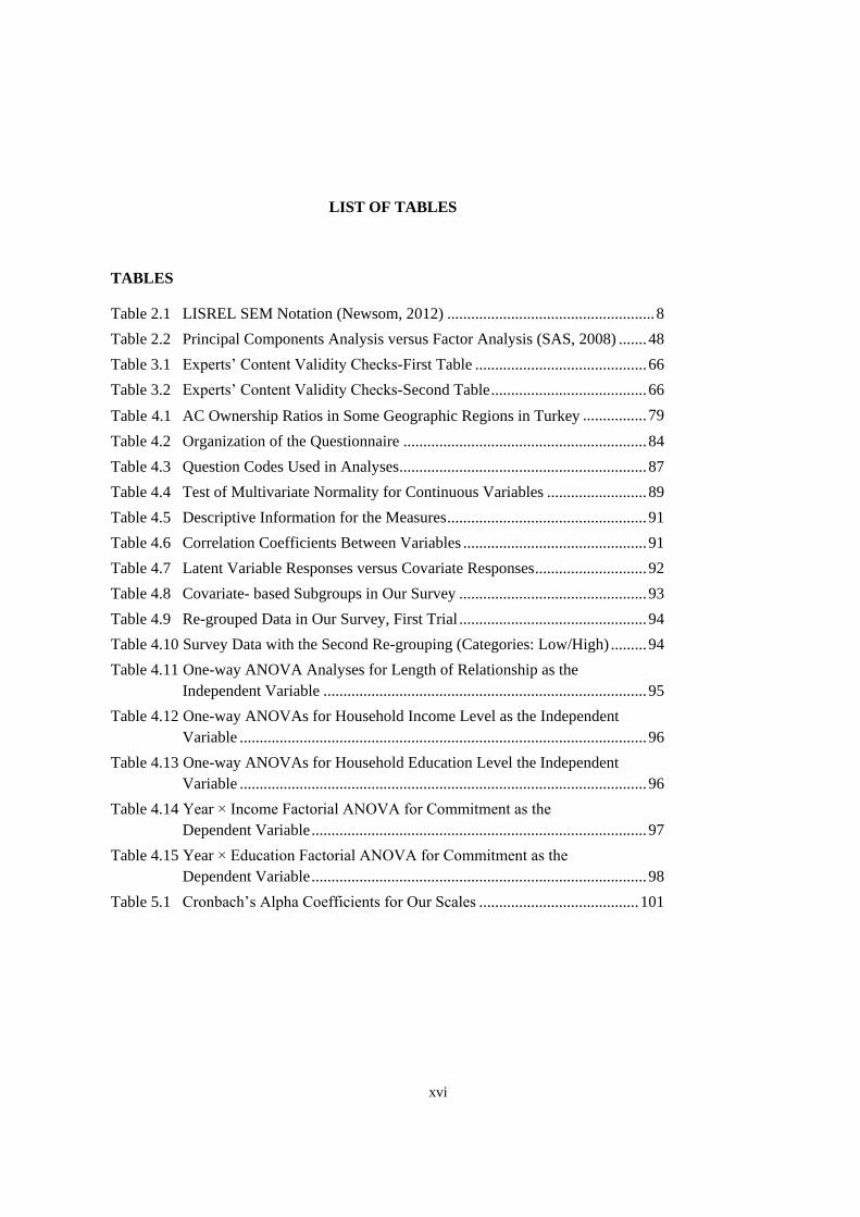
LIST OF TABLES ...................................................................................................... xvi

CHAPTERS

1. INTRODUCTION ..................................................................................................... 1

2. LITERATURE SURVEY AND BACKGROUND ................................................... 7

2.1. LITERATURE SURVEY ON STRUCTURAL EQUATION MODELING ........ 7

2.2. STEPS OF STRUCTURAL EQUATION MODELING ....................................... 8

2.2.1. SPECIFICATION OF STRUCTURAL EQUATION MODELS ................ 9

2.2.2. ESTIMATION IN STRUCTURAL EQUATION MODELS .................... 11

2.3. ASSUMPTIONS UNDERLYING STRUCTURAL EQUATION

MODELS ............................................................................................................. 15

2.4. LONGITUDINAL DATA ANALYSIS WITH STRUCTURAL

EQUATION MODELS ........................................................................................ 16

2.5. STRUCTURAL EQUATION MODELS WITH FORMATIVE LATENT

VARIABLES AND COVARIATES (MIMIC MODELS) .................................. 18

2.6. LITERATURE SURVEY ON CUSTOMER LOYALTY MODELS.................. 23

2.6.1. DEFINITIONS OF LOYALTY AND SATISFACTION .......................... 23

2.6.2. IMPORTANCE OF LOYALTY IN CUSTOMER RELATIONSHIP

MANAGEMENT ....................................................................................... 25

2.6.3. LOYALTY MODELS IN LITERATURE ................................................ 25

2.7. SCALING AND VALIDATION ......................................................................... 34

2.7.1. LITERATURE REVIEW ON SCALES IN OUR RESEARCH

COMPANY IMAGE (REPUTATION) CONSTRUCT ............................ 35

2.7.2. VALIDATION OF SCALES ..................................................................... 42

2.7.3. EXPLORATORY FACTOR ANALYSIS FOR SCALING ...................... 47

2.8. LITERATURE REVIEW OF QUESTIONNAIRE DESIGN .............................. 50

2.8.1. UNIDIMENSIONALITY .......................................................................... 50

x

2.8.2. OPTIMAL NUMBER OF RESPONSE CATEGORIES AND

NUMBER OF CHOICES ........................................................................... 51

2.8.3. TRANSLATION / BACKTRANSLATION OF SCALES IN

CROSS-CULTURAL RESEARCH ........................................................... 52

2.8.4. SAMPLE SIZE CONSIDERATIONS ....................................................... 52

2.8.5. SAMPLE SIZE FOR PROPER STATISTICAL SOLUTIONS ................ 52

2.8.6. SAMPLE SIZE AND FIT INDICES FOR SEM ....................................... 53

2.8.7. SAMPLE SIZE AND STATISTICAL POWER IN STRUCTURAL

EQUATION MODELING ......................................................................... 55

2.8.8. SAMPLE SIZE CALCULATIONS BASED ON FACTOR

ANALYSIS ................................................................................................ 55

2.8.9. SAMPLE SIZE CALCULATIONS BASED ON SAMPLING

THEORY .................................................................................................... 56

2.8.10. FIT INDICES FOR STRUCTURAL EQUATION MODELS ................. 57

3. MODELING AND ANALYSIS STRATEGIES ..................................................... 63

3.1. THE MODEL SPECIFICATION .................................................................... 63

3.2. SPECIFICATION OF OUR MEASUREMENT MODEL ............................. 64

3.3. SPECIFICATION OF A STRUCTURAL MODEL ....................................... 64

3.3.1. SPECIFICATION OF THE EXTENDED STRUCTURAL MODEL

WITH COVARIATES .................................................................................... 64

3.3.2. HYPOTHESIZED RELATIONS BETWEEN COVARIATES AND

LATENT VARIABLES IN THE BASE MODEL .......................................... 65

3.4. CONTENT VALIDITY OF HYPOTHESIZED RELATIONS ...................... 65

3.5. DETAILED EXPLANATION OF OUR RESEARCH MODEL .................... 67

3.5.1. THE STRUCTURAL MODEL .................................................................. 67

3.5.2. STRUCTURAL MODEL EQUATIONS ................................................... 68

3.5.3. THE MEASUREMENT MODEL .............................................................. 68

3.5.4. MEASUREMENT MODEL EQUATIONS .............................................. 69

3.5.5. MATRIX EQUATIONS FOR THE FULL MODEL ................................. 70

3.6. HYPOTHESIZED MODERATED RELATIONS AS A FURTHER

EXTENSION OF THE MODEL ..................................................................... 71

3.7. ANALYSIS STAGES ..................................................................................... 72

3.8. LONGITUDINAL MODELING POSSIBILITIES AND REASONS OF

NOT ADAPTING THIS APPROACH ........................................................... 72

3.9. MULTIGROUP MODELING POSSIBILITIES ............................................. 75

3.9.1. MULTIGROUP MODELS AS EXTENSIONS OF MIMIC

MODELS ................................................................................................... 75

3.10. DIRECT EFFECT OF LENGTH OF RELATIONSHIP ............................... 76

xi

3.11. EXPLORATORY FACTOR ANALYSIS WITH PILOT

QUESTIONNAIRE DATA .......................................................................... 76

3.12. PRIOR MEDIATION AND MODERATION ANALYSES ....................... 76

4. DATA COLLECTION AND ANALYSIS .............................................................. 79

4.1. SAMPLING DESIGN ..................................................................................... 79

4.2. DATA COLLECTION ................................................................................... 80

4.3. QUESTIONNAIRE DESIGN ......................................................................... 80

4.4. COVARIATES USED IN THE MEASUREMENT MODEL ....................... 81

4.4.1. CONTINUING RELATIONSHIP COVARIATES ................................ 81

4.4.2. PRODUCT UPGRADE/CONTRACT RENEWAL DECISION

COVARIATES ........................................................................................ 82

4.4.3. COVARIATES MEASURING DEMOGRAPHIC

CHARACTERISTICS............................................................................. 82

4.5. BACKGROUND AND ORGANIZATION OF THE QUESTIONNAIRE ...... 82

4.6. DATA ANALYSIS ......................................................................................... 88

4.6.1. DATA SCREENING ............................................................................... 88

4.6.2. NEGATED QUESTIONS ....................................................................... 90

4.7. BASIC DESCRIPTIVE STATISTICS ............................................................ 90

4.8. COVARIATES’ EFFECTS ON LATENT VARIABLES .............................. 92

4.9. COVARIATE-BASED GROUPINGS ............................................................ 93

5. FINDINGS ............................................................................................................... 99

5.1. STRUCTURAL EQUATION MODELING STEPS ............................................ 99

5.2. TESTED MODELS ............................................................................................ 100

5.3. MEASUREMENT MODEL ANALYSES ......................................................... 100

5.4. STRUCTURAL MODEL ANALYSES ............................................................. 104

5.4.1. HYPOTHESIZED RELATIONS BETWEEN LATENT VARIABLES ... 105

5.4.2. RESULTS ................................................................................................... 107

5.5. COVARIATE- EXTENDED STRUCTURAL MODELS ................................. 110

5.6. MODERATED STRUCTURAL EQUATION MODELS ................................. 114

5.6.1. LENGTH OF RELATIONSHIP MODERATING SATISFACTION-

LOYALTY PATH ...................................................................................... 114

5.6.2. LENGTH OF RELATIONSHIP MODERATING PERCEIVED

QUALITY-PERCEIVED VALUE PATH ................................................. 115

5.6.3. LENGTH OF RELATIONSHIP MODERATING COMMUNICATION

- CUSTOMER SATISFACTION PATH ..................................................... 116

5.6.4. HOUSEHOLD’S INCOME LEVEL MODERATING

SATISFACTION-LOYALTY PATH ........................................................ 117

xii

5.6.5. HOUSEHOLD’S INCOME LEVEL MODERATING PERCEIVED

QUALITY PERCEIVED VALUE PATH .................................................. 117

5.6.6. HOUSEHOLD’S EDUCATION LEVEL MODERATING

COMMITMENT-LOYALTY PATH ......................................................... 118

5.6.8. MODERATION EFFECTS TESTED BY SPSS PROCESS MACRO ...... 119

5.6.9. MODERATION EFFECTS TESTED BY INTERACTION MODELS .... 120

5.6.9.1. THE METHOD ................................................................................... 120

5.6.9.2. MODERATED STRUCTURAL MODELS ....................................... 121

5.6.10. DIRECT AND INDIRECT EFFECTS OF MARKER ITEMS ................ 127

6. STRATEGIC IMPLICATIONS AND FUTURE RESEARCH

DIRECTIONS ....................................................................................................... 131

6.1. AIM OF THE STUDY .................................................................................. 131

6.2. SUMMARY OF OUR FINDINGS AND STRATEGY

RECOMMENDATIONS .............................................................................. 131

6.2.1. DEVELOPING SURVEYS TO MEASURE CONSUMER

ATTITUDES ......................................................................................... 131

6.2.2. CONSUMER RESPONSES ON LENGTH OF UTILIZATION OF

AN AC PRODUCT ............................................................................... 132

6.2.3. CONSUMER RESPONSES BASED ON HOUSEHOLD

INCOME LEVEL .................................................................................. 132

6.2.4. CONSUMER RESPONSES BASED ON SIMULTANEOUS

EFFECTS OF LENGTH OF UTILIZATION AND HOUSEHOLD

INCOME LEVEL .................................................................................. 133

6.2.5. CONSUMER RESPONSES BASED ON LENGTH OF

UTILIZATION AND HOUSEHOLD EDUCATION LEVEL ............. 133

6.3. CONSUMER PERCEPTIONS AND FUTURE RESEARCH

DIRECTIONS ............................................................................................... 133

6.3.1. CONSUMERS’ SATISFACTION WITH A PRODUCT ..................... 133

6.3.2. CONSUMERS’ LOYALTY TO A PRODUCT / BRAND ................... 134

6.3.3. CONSUMERS’ EXPECTATIONS FROM A PRODUCT/BRAND .... 134

6.3.4. CONSUMERS’ TRUST IN A PRODUCT/BRAND ............................ 135

6.3.5. CONSUMERS’ INSENSITIVITY TO COMPETITIVE

OFFERINGS .......................................................................................... 135

6.3.6. CONSUMERS’ VALUE PERCEPTION FOR AN AC PRODUCT .... 136

6.3.7. CONSUMERS’ COMMITMENT TO A PRODUCT/BRAND ............ 136

6.4. RESPONSE PREDICTION FOR MARKETING STRATEGIES................. 137

6.5. ADDITIONAL FUTURE RESEARCH DIRECTIONS ................................ 138

xiii

REFERENCES .......................................................................................................... 139

APPENDICES

A THE QUESTIONNAIRE FORM .......................................................................... 151

B THE LIST OF LISREL .......................................................................................... 157

C SPSS PROCESS OUTPUT .................................................................................... 159

D LIST OF TECHNICAL TERMS ........................................................................... 161

CURRICULUM VITAE ............................................................................................ 163

xiv

LIST OF FIGURES

FIGURES

Figure 2.1 A Typical Structural Equation Model (Rigdon, 1996) ........................... 7

Figure 2.2 A Measurement Model (Rigdon, 1996) .................................................. 9

Figure 2.3 A Structural Model (Rigdon, 1996) ...................................................... 10

Figure 2.4 Ferron and Hess’s (2007) Example Problem ........................................ 13

Figure 2.5 Identification of SE Models (Hannemann, 1999) ................................. 14

Figure 2.6 Longitudinal Models with Two Measurement Points and Group

Effects (McArdle, 2009) ....................................................................... 16

Figure 2.7 Multivariate Two Measurement Occasion Structural Models

(McArdle, 2009) ................................................................................... 17

Figure 2.8 Multivariate Multiple Measurement Occasion Structural Models

With Time Series Concepts (McArdle, 2009) ...................................... 18

Figure 2.9 Reflective and Formative Measurement Models (Diamantopulos,

1999) ..................................................................................................... 19

Figure 2.10 Christensen et al.’s (1998) MIMIC model ............................................ 20

Figure 2.11 A MIMIC Model (Pynnonnen, 2010) ................................................... 21

Figure 2.12 A MIMIC Model’s Path Diagram ......................................................... 21

Figure 2.13 A MIMIC Model with three latent variables and nine- indicator

Variables (Pynnonnen, 2010) ............................................................... 22

Figure 2.14 Customer Satisfaction- Customer Loyalty Path Model (Fornell,

1996) ..................................................................................................... 25

Figure 2.15 Yu et al.’s (2005) Customer Satisfaction- Customer Loyalty Path

Model for Lexus Cars ....................................................................... 26

Figure 2.16 European Customer Satisfaction Index Model (Lars et al., 2000) ........ 27

Figure 2.17 ECSI Model Extended to Include Trust and Communication (Ball

et al. 2004) ............................................................................................ 27

Figure 2.18 Türkyılmaz and Özkan (2007)’s Customer Satisfaction Loyalty

Model for Turkish Mobile Phone Industry ........................................... 29

Figure 2.19 Habits as an Antecedent of Loyalty (Andreassen and Lindestad,

1998) ..................................................................................................... 30

Figure 2.20 Effects of Different Loyalty Attitudes on Online Word-of-Mouth

Behaviors of Customers (Roy et al., 2009) ........................................... 31

Figure 2.21 The “Gaps” Service Quality Model (Zeithaml, 1988) .......................... 32

Figure 2.22 Extended “Gaps” Service Quality Model (Zeithaml et al., 1988) ........ 33

Figure 2.23 Commitment Behavior and Advocacy Intentions (Fullerton,

2011) ..................................................................................................... 40

Figure 2.24 A typical factor analysis path model (Pedersen et al., 2009) ................ 49

xv

Figure 2.25 Three Common Fit Indices (Iacobucci, 2010) ....................................... 54

Figure 2.26 Moderated Regression ........................................................................... 58

Figure 2.27 A Moderated Regression Path Model .................................................... 58

Figure 2.28 An Interaction Plot ................................................................................ 59

Figure 2.29 A Moderated SE Model (Kenny and Judd, 1984) ................................. 59

Figure 2.30 A SE Model with Scaling Indicators (Hayduk and Littvay, 2012) ....... 60

Figure 3.1 Suggested Path Model for the Research Problem ................................. 67

Figure 3.2 A Sub-model of the Research Problem ................................................. 68

Figure 3.3 A Sub-model of our Research Problem ................................................. 69

Figure 3.4 A Confirmatory Factor Analysis Sub-model ......................................... 69

Figure 3.5 A Full SE Model (Rigdon, 1996) .......................................................... 70

Figure 3.6 An Extended SEM with Covariates (MIMIC Model) ........................... 70

Figure 3.7 Covariates Modeled with a Pseudo-Latent (Phantom) Variable ........... 72

Figure 3.8 SPSS PROCESS Tool’s Model for testing mediation effects

(Hayes, 2012) ........................................................................................ 77

Figure 3.9 SPSS- PROCESS Tool’s Model for testing moderation effects

(Hayes, 2012) ........................................................................................ 77

Figure 4.1 Length of Interaction - Household Income Level – Commitment

Interaction .............................................................................................. 97

Figure 4.2 Length of Relationship-Household Education Level-Commitment

Interaction .............................................................................................. 98

Figure 5.1 CFA Model’s T-Values ....................................................................... 105

Figure 5.2. Structural Model’s T- Values .............................................................. 110

Figure 5.3 Covariate- Extended Structural Model ................................................ 113

Figure 5.4 Satisfaction-Loyalty – Length of Relationship Interaction ................. 115

Figure 5.5 Perceived Value-Perceived Quality and Length of Relationship

Interaction ............................................................................................ 116

Figure 5.6 Communication-Customer Satisfaction and Length of

Relationship Interaction ...................................................................... 116

Figure 5.7 Satisfaction-Loyalty – Household Income Level Interaction .............. 117

Figure 5.8 Perceived Quality-Perceived Value and Household Income Level

Interaction ............................................................................................ 118

Figure 5.9 Commitment- Loyalty-Household Education Level Interaction ......... 118

Figure 5.10 Perceived Quality-Perceived Value and Household Education

Level Interaction ................................................................................. 119

Figure 5.11 A Moderated SEM (Kenny and Judd, 1984) ....................................... 120

Figure 5.12 Our Moderation Model for a Hypothesized Path ................................ 121

Figure 5.13 Moderation Model 1 ............................................................................ 124

Figure 5.14 Moderation Model 2 ............................................................................ 126

xvi

LIST OF TABLES

TABLES

Table 2.1 LISREL SEM Notation (Newsom, 2012) .................................................... 8

Table 2.2 Principal Components Analysis versus Factor Analysis (SAS, 2008) ....... 48

Table 3.1 Experts’ Content Validity Checks-First Table ........................................... 66

Table 3.2 Experts’ Content Validity Checks-Second Table ....................................... 66

Table 4.1 AC Ownership Ratios in Some Geographic Regions in Turkey ................ 79

Table 4.2 Organization of the Questionnaire ............................................................. 84

Table 4.3 Question Codes Used in Analyses .............................................................. 87

Table 4.4 Test of Multivariate Normality for Continuous Variables ......................... 89

Table 4.5 Descriptive Information for the Measures .................................................. 91

Table 4.6 Correlation Coefficients Between Variables .............................................. 91

Table 4.7 Latent Variable Responses versus Covariate Responses ............................ 92

Table 4.8 Covariate- based Subgroups in Our Survey ............................................... 93

Table 4.9 Re-grouped Data in Our Survey, First Trial ............................................... 94

Table 4.10 Survey Data with the Second Re-grouping (Categories: Low/High) ......... 94

Table 4.11 One-way ANOVA Analyses for Length of Relationship as the

Independent Variable ................................................................................. 95

Table 4.12 One-way ANOVAs for Household Income Level as the Independent

Variable ...................................................................................................... 96

Table 4.13 One-way ANOVAs for Household Education Level the Independent

Variable ...................................................................................................... 96

Table 4.14 Year × Income Factorial ANOVA for Commitment as the

Dependent Variable .................................................................................... 97

Table 4.15 Year × Education Factorial ANOVA for Commitment as the

Dependent Variable .................................................................................... 98

Table 5.1 Cronbach’s Alpha Coefficients for Our Scales ........................................ 101

1

CHAPTER 1

INTRODUCTION

Customer relationship management studies have shown that, in today’s world,

companies’ profits can best be increased by elevating customers’ loyalties or by

increasing number of loyal customers. An ever increasing number of publications are

focusing on modeling factors affecting customer loyalty. Manufacturers and marketing

professionals of durable goods have also been experiencing an increasing need for

developing loyalty strategies and campaigns.

Modeling of customer loyalty for durable consumption goods and particularly for heating,

ventilating and air-conditioning products has not been studied enough in either the

scientific literature or in industrial practice. Therefore, customer relationship professionals

lack a reliable and valid framework to develop policies and campaigns to improve loyalty.

Such models should be different from their counterparts in view of the complexity of the

factors affecting loyalty and its time-based structure. Existing studies are mostly

concentrated on fast- consumption goods and services. Findings of these studies cannot

directly be applied to durable goods’ consumption cases due to specific nature of the

latter scenarios. Renewal phases, long utilization periods and infrequent replacement

needs are some of the differentiating characteristics of durable goods’ consumption

settings. Consumer behavior for these goods should be studied differently than settings of

fast-consumption goods or services.

We have formulated our research question as “the study of the antecedents and

consequences of customer satisfaction and customer loyalty for residential air-

conditioners”. Air-conditioners (AC) are also durable goods but they have special

consumption patterns. A typical consumer decision-making process which involves the

pre-purchase, purchase and post-purchase evaluation stages again exist for AC devices.

Additionally, the post-consumption period can involve varied levels of customer attitudes

for seasonal utilization. Many attitudinal variables can form, evolve or disappear in the

life-cycle of an AC device. Therefore, this study is unique in filling gaps in the literature

and in providing support to industrial practice. The weaknesses of the literature and our

original contributions can be summarized as follows:

- Consumer research for durable goods is limited to scale development that is

developing questionnaires for some categories of technical criteria related to the usage

of the products or study of antecedents of satisfaction in a restricted context. In our

research, however, a comprehensive modeling is done, which includes, but not

restricted to questionnaire development.

2

- Existing literature on loyalty for durable goods is limited to customer satisfaction

index models and satisfaction modeling for cars and white goods and factor analysis

study of durable goods. Our research provides a framework which can be used to

develop satisfaction indices and also models that can be adapted to all kinds of

durable goods.

o In the literature, structural equation modeling (SEM), regression and

stochastic approaches are used as modeling and analysis tools. The factors

affecting the consumption of these goods are studied using factor analysis or

cross-sectional modeling approaches. The inherent affecting variables such as

length of relationship with the supplier, household’s education and income

levels are not handled as additional factors. Our research uses SEM with

covariates and this is more comprehensive than stand-alone regression

modeling, factor analysis or cross sectional modeling approaches.

o Limited number of latent variables is studied in existing customer satisfaction

–loyalty models. In these models, intermediary factors affecting the

relationship between customer satisfaction and loyalty are not evaluated. In

real situations, this relationship is generally observed indirectly. Time-

relevancy due to habits, meeting the expectations and other consumer

perceptions are not studied in detail. Consumers’ consumption decisions are

shaped by inconsistency in brand loyalty attitudes and with effect variables

such as tendency towards alternative firms and different behavior patterns

resulting in consumption periods that are extended in a long period of time. In

this research, time is considered as an effect and grouping variable together

with an integrated model of latent variables. Ten different behavioral factors

are studied together with some covariates. This has resulted in a large-scale

SEM. The covariates include both demographic and also usage variables. The

usage variable is the length of relationship with the retailer. This is a new

approach for loyalty modeling and is only studied in a service consumption

setting in the literature. Wang and Wu (2012) have studied the effect of

relationship length on the customer loyalty for hair salons. Our model

incorporates this into durable goods’ consumption settings.

o Past research shed some light on the relation between length of relationship

and customer behavior in different consumption settings. Chiao (2008) has

studied the relations of six factors for banking industry and for different

groups of customers. Thus they have studied the length of relationship through

two groups of customers and the variable is not directly included in the model.

Two different models are hypothesized and tested; Liu et al. (2005) have

hypothesized and tested SEM’s for two groups of buyers involved in

organizational buying-selling environment for financial staffing industry. They

study four latent variables. Sabiote and Sergio (2009) have examined the

influence of employees’ social regard on customer satisfaction, trust and word

of mouth for two service industries. They include “length of relationship” as a

moderating variable. They do not study loyalty as a separate variable. Bell et

al. (2005) have studied the effects of customer expertise and other variables

3

on loyalty attitudes of customers in financial advisory services’ industry.

Many researchers study antecedents of loyalty for consumption of goods with

limited number of variables and /or covariates. Suh and Yi (2006) have

studied moderating effects of product involvement on antecedents of customer

loyalty. They have formulated a five-factor model with loyalty and its four

antecedents. This model does not include covariates. Krishnan (2011) has

studied the linear relations between supplier characteristics and customer

loyalty for durable household goods. In this study, regression analysis

framework has been used with only technical variables and not classical

marketing constructs.

o In existing literature, loyalty, its a priori or a posteriori variables are defined in

terms of “fast-moving consumption” attitudes. Customer loyalty is defined as

a “repeated purchasing” behavior. This definition is valid only in “fast-moving

consumption” scenarios. However, for purchase of durable goods and in

provision of related services, recommendation and switching attitudes are also

observed. These latter variables are included in our model as separate factors.

Additionally, loyalty is measured with both attitudinal and also behavioral

dimensions. Different behavioral patterns in the course of long-lasting

consumption processes are not discussed. The loyalty variable, predecessors

and consecutive variables have been described only according to rapid

consumption pattern. Customer loyalty has been defined as a recurrent

purchase. This is a valid assumption only in rapid consumption scenarios.

Recommendation to others is frequently observed in consumption of durable

commodities and concerned services, and a brand change behavior in service

purchase settings.

- Satisfied but disloyal customers who are frequently encountered in durable goods’

consumption settings are not examined in existing models. Several customers satisfied

with the product are not loyal to the brand and can shift to alternative brands. This

behavior can be examined only by inclusion of intermediary variables. Variables such

as trust (brand/corporation trust), shifting to alternatives, corporate image which affect

the prospective consumption decisions in purchases of expensive products used for a

long time, communication of the consumer with the seller firm, and future prospects

have not been included in the model. Implied variables can differ in different

consumption phases (pre-purchase, purchase and post-purchase.

- For durable products, customer satisfaction and related variables can evolve or

disappear over time. "Customers require experience with a product to determine how

satisfied they are with it" (Anderson et al. 1994). A detailed analysis can only be

achieved with inclusion of “length of relationship” as a control variable. We use this

together with other covariates and latent variables to examine the effects of short and

long-term usage of an AC product on customer perceptions.

- In marketing literature, commitment has widely been acknowledged to be an integral

part of any long-term business-to- business relationships. However, commitment is

also an essential underlying factor of long-term customer-retailer-producer

relationships. This is why we are including “commitment” as a separate variable in

our conceptual model. Loyalty and commitment are modeled together as long-term

relationship variables in customer- retailer- producer relationships.

- Our research is of unique value in terms of future customer satisfaction index

development studies since a limited and different number of implied variables are

studied in index models in the literature. Intermediary factors to affect satisfaction –

loyalty relation are not considered in the existing models. Actually, this relation

4

frequently happens indirectly rather than directly. Consumers can decide under

varying effects such as inconsistency in relation with brand loyalty and shifting to

alternative firms.

- Existing literature in industrial engineering (IE) and operations management (OM)

contains models related to supply chain problems, product development applications,

modeling of investment projects, and satisfaction-loyalty relations for

telecommunications and internet industries. Kwang et al. (2007) have studied

satisfaction-loyalty link and their technological predecessors for internet technologies.

The model is a longitudinal study of two latent variables with many indicators. To the

best of our knowledge, existing IE and OM literature does not contain a study of

consumer behavior for durable goods.

- Total quality management aims to serve for designing processes and systems to deliver

superior quality products for better customer satisfaction. “Customer satisfaction” is

the major emphasis for total quality management (TQM) studies. Existing TQM

research does not contain a comprehensive framework for studying satisfaction,

loyalty, predecessors and successors. Satisfaction and loyalty are closely related in

consumer behavior research. Thus our study will guide future TQM studies in forming

the integrative frame of satisfaction and loyalty for industrial processes.

o AC devices are expensive durable goods. Thus consumers’ income level is

expected to be a major controlling variable for consumer behavior. Our model

includes this as as control variable.

o Many residential AC users are using these devices on a seasonal basis. Some

variables affecting satisfaction and loyalty forms only after two or three seasons

(years). In our research, the effect of time is studied as a separate and also as an

interaction variable.

There are many structural equations modeling applications applied to customer

satisfaction modeling in different Turkish industries. These are in banking products

services (with existing SEMs and not with new approaches), tourism services (with

limited number of variables), health services, telecommunications services (with a

limited number of variables or only for scale construction), Turkish customer

satisfaction index survey (adapted from American Customer Satisfaction Index

studies and is not a new modeling study). These studies do not include consumption

of a specific durable product (Yılmaz and Çelik (2005), Yılmaz et al. (2011),

Türkyılmaz and Özkan (2007), Özer and Aydın (2004), Erdem et al. (2008), Duman

(2003)). Our study has a unique value as to customer satisfaction-loyalty studies in

Turkey. Unique value of our study for research and industrial practice in Turkey are

detailed below:

1. Comparative Unique Value with Customer Satisfaction/Loyalty Models for Banking

Products and Services

A limited and different number of implied variables are studied in reviewed models.

Intermediary factors to affect satisfaction - loyalty relation are not considered. Long-term

customer expectation attitudes are not studied in the models. Existing measurement

models like “Service Quality Index” (SERVQUAL) have been used. Period-based

customer communication and expectations are not discussed in these models.

2. Comparative Unique Value with Customer Satisfaction /Loyalty Models for Tourism

Services

A limited and different number of implied variables are studied in reviewed models.

Long-term customer expectation attitudes are not studied in the models. Customer

5

satisfaction has been discussed as the intermediary of the loyalty attitudes. Other

intermediary factors to affect satisfaction - loyalty relation are not considered.

3. Comparative Unique Value with Customer Satisfaction /Loyalty Models for Health

Services

Intermediary factors to affect satisfaction - loyalty relation are not considered. Long-

term customer expectation attitudes are not studied in the models. Studies are held in

the form of multiple group comparisons.

4. Comparative Unique Value with Customer Satisfaction /Loyalty Models for

Communication Product / Services

Intermediary factors to affect satisfaction – brand loyalty relation are not considered.

Long-term customer expectation attitudes are not studied in the models. Türkyılmaz et

al. (2007) have developed satisfaction index models for Turkish Telecom and Turkish

mobile telecommunications industries with less number of latent variables than in our

model.

5. Comparative Unique Value with Turkish Customer Satisfaction Index Modeling

There is a study is conducted by Turkish Quality Association. American Customer

Satisfaction Index (ACSI) Model has been taken as a basis. Intermediary factors to

affect satisfaction - loyalty relation are not considered. Long-term customer behavior

patterns are not studied in this model. Limited number of variables (6 implied and 17

indicator variables) has been modeled. Effect variables are not included in the model.

6. Comparative Unique Value with Formation of Customer Satisfaction Index Model

for Cellular Phone Use

Intermediary factors to affect satisfaction - brand loyalty relation are not considered.

Long-term customer expectation attitudes are not studied in the models. Current

customer satisfaction index models are reviewed.

7. Unique Value in terms of Modeling of Customer Satisfaction – Customer Loyalty

Problems via Structural Equations Method

“Multiple-Indicator Multiple-Cause” (MIMIC) models constitute a structural equality

modeling approach used to study simultaneous presence of causal and indicator

variables. Several effect variables, differences in intercept and factor averages can be

examined in single framework using these models. A comprehensive MIMIC modeling

study has not been conducted in the prior studies.

One of the aims of our research can be stated as to fill gaps in existing research for

consumers’ goods. The second and equally important aim of our research is to develop a

compact body of strategies for guiding marketing experts working in HVAC and other

durable goods’ industries. To the best of our knowledge, no previous study has

investigated this many constructs and covariates in a single model’s framework.

This report is organized in six chapters and appendices. Second chapter contains a

detailed explanation of SEM techniques and their applications. Third chapter discusses

the research problem and modeling strategies. Fourth chapter details data collection

methods and organization of the questionnaire. Fifth chapter contains data analyses and

findings. Sixth chapter contains scientific/ strategic conclusions and future research

directions. Appendices contain preliminary statistical analyses, the questionnaire forms, a

list of LISREL notations and a glossary of technical terms.

6

7

CHAPTER 2

LITERATURE SURVEY AND BACKGROUND

2.1. LITERATURE SURVEY ON STRUCTURAL EQUATION MODELING

Structural Equation Modeling (SEM) is a statistical technique to study interrelated

regression equations containing “latent” variables, “indicator” variables and side

variables. The latent variables are also referred to as constructs and these represent

underlying dimensions in a model. Precisely, these are “abstraction” variables which are

assessed through their measurable variables called “indicator” variables. Human

perception variables like emotions, satisfaction and trust are typical examples of

“abstracted” variables. These can only be measured through measurable variables which

are their “indicator” variables. The paths connecting each pair of variables are actually

regression equations.

Structural equation modeling (SEM) is a combination of three statistical techniques; factor

analysis, simultaneous equation modeling and path analysis. The first commonly known

factor analysis application dates back to Spearman (cited by Kaplan, 2000) for modeling

common characteristics of mental traits. Other researchers (Joreskog and Lawley as cited

by Kaplan, 2000) develop maximum likelihood-based approach to factor analysis. The

second track in history of SEM is the development of simultaneous equations modeling in

genetics and econometrics. Finally, Wright (1921) is the first researcher to devise path-

analytic depiction of simultaneous equations.

A typical SE model looks like follows:

Figure 2.1 A Typical Structural Equation Model (Rigdon, 1996)

8

In the above model, the latent variables are depicted by ovals and indicator variables are

represented by boxes. Y is the vector of indicators of endogenous latent variables; ηi, i=1,

2, 3. Similarly X is the vector of indicators of exogenous latent variables; ξ i, i=1, 2. εi,

i=1,2,..,7 is vector of measurement errors of indicator variables. There are also the

disturbance terms which are denoted by ζi, i=1, 2, 3 for the three endogeneous latent

variables. Γ and β are the vectors of path coefficients between the latent variables. Greek

and Latin letters are used to indicate variables in SE models. A full list of SEM notations

is given in Table 2.1 (Newsom, 2012). These are also called Linear Structural Relations

(LISREL) notations.

Table 2.1 LISREL SEM Notation (Newsom, 2012)

Parameter symbol

(lowercase Greek Letter)

Matrix symbol

(capital Greek letter) Description

λx, λy Λx , Λy Loadings for exogenous and

endogenous latent variables

φ Φ variances and covariances of exogenous latent variables

ψ Ψ covariances among endogenous disturbances

γ Γ causal path from exogenous to endogenous variables

β Β path coefficients’ matrix

------ A path coefficients’ matrix

δ, ε Θδ (also named as Δ), Θε measurement errors for exogenous and endogenous

variables

ξ not used as matrix, only in

naming factors exogenous latent variables

η not used as matrix, only in

naming factors endogenous latent variables

ζ not used as matrix, only in

naming disturbance disturbances for endogenous variables

x, y not used as matrices, only

as separate variables

indicators(measured variables) for exogeneous and

endogenous latent variables

------ Σ Covariance matrix

Unlike multivariate regression analysis, a variable in a SE model can become a predictor

and also an outcome variable simultaneously. This is clearly observed in Figure 2.1.

Measurement errors are also taken into account in all of the relationships.

2.2. STEPS OF STRUCTURAL EQUATION MODELING

Bollen (1989) gives the modeling steps in SEM as follows:

A. Specification

B. Implied Covariance Matrix

C. Identification

D. Estimation

E. Testing and Diagnostics

F. Re-specification

9

Steps A and B are mostly combined as “specification” in SEM literature. In step A, we

state the hypotheses and specify a model a priori. In this step, the model’s covariance

matrix is calculated according to the fitted model’s features; the paths, the correlations and

the disturbances.

In step C, we try to estimate all unknown parameters with the assumed measurement

equations until the model becomes identified. Even if the model is identified we should

check for rational results.

In steps D and E, estimate the parameters of the model with the actual collected data. In

step F, the model is revised if the model fit is to be improved. All SEM software provides

modifications for possible improvements. These can be combined with the researcher’s

judgments for the optimal modifications.

2.2.1. SPECIFICATION OF STRUCTURAL EQUATION MODELS

Specifying a structural equation model is basically different from formulating one or more

regression equations. We have a number of independent variables and another set of

dependent variables which are linked through a complex series of equations. Figure 2.1

depicts a typical SE model. In this model, the boxes represent the measured items (which

correspond to “questionnaire items”) and the circles correspond to the hypothesized latent

variables or the underlying factors. This model contains two parts:

1. Measurement Model

2. Structural Model

SE model specification starts with specifying the measurement model as given in Figure

2.2. The latent variables are the factors and the paths between the latent variables and

boxes are specified. These paths are the hypothesized “item loading”s.

Figure 2.2 A Measurement Model (Rigdon, 1996)

10

Measurement model is analyzed and the following set of measurement equations is

obtained :

(2.1)

Here, y represents the p × 1 vector of indicator variables of exogenous latent variables, ξ1

and ξ2.

Second step of an SE model specification process is the hypothesizing of structural paths

between latent variables. This is depicted in Figure 2.3.

Figure 2.3 A Structural Model (Rigdon, 1996)

The above model is analyzed and the following set of structural equations is obtained:

(2.2)

Combining the two sub-models we obatain the full model in Figure 2.1. This model is

specified as an SE model with five latent variables and twelve indicator variables. The

model is represented by the following set of measurement equations:

ξη Δ 0 ζ

xη = A + Γ Γ Γ + 1x1 x2ξy 0 Ψ εx2

(2.3)

In the above sets of equations, is the m×1 vector of latent endogenous variables, y is the

px1 vector of measurable endogenous variables, A is the (m+p) × (m+p) matrix of path

coefficients of causal links connecting endogenous variables to all other endogenous

variables, Γξ is the (m +p) × n matrix of path coefficients of paths connecting endogenous

variables to exogenous observed variables, Γx1 is the (m +p) × q1 matrix of path coefficients

of paths connecting endogenous variables to exogenous observed variables, x1 (q1 ×1), Γx2 is

the (m +p) × q2 matrix of path coefficients of paths connecting endogenous variables to

11

exogenous observed variables, x2 (q2 ×1), (q1 + q2) being equal to q, the total number of

measured variables. The principle diagonal of A contains zeros because no endogenous

variable can be a cause of itself. is the m × 1 vector of disturbance random variables on the

latent endogenous variables. is the matrix of path coefficients relating all variables to their

measurement errors (for indicators) or disturbances(for latent variables). Ψ is a p × p

diagonal matrix of structural coefficients relating measurable endogenous variables to

exogenous disturbance variables. x is the vector of exogenous indicators.

The properties of the above model are as follows:

All of the latent variables are connected to their indicator variables.

Latent variables have disturbance terms.

Latent variables are measured through their indicators.

Indicators refer to data collected through questionnaires and they have measurement

errors.

Measurement errors can be correlated. This depends on researcher’s assumptions and

required modifications.

Disturbance terms cannot be correlated with measurement error terms.

2.2.2. ESTIMATION IN STRUCTURAL EQUATION MODELS

In structural equation modeling, we are trying to calculate values for the parameters of the

problem so that the “implied covariance” that is the model-fitted covariance matrix is as

close as possible to the observed covariance matrix. Bollen (1989) states the fundamental

hypothesis as follows:

Population covariance matrix = Model Implied covariance matrix

The hypothesis can thus be written as:

Σ = Σ (θ) (2.4)

Where θ is the vector of parameters estimated in the fitted model and Σ is the real population’s

covariance matrix (dimension for θ can be calculated as the sum of number of path

coefficients, factor loadings and covariance terms in the fitted model). The aim is to get the

values of these two matrices as close as possible. The most common estimation method is

maximum likelihood estimation and it is based on multivariate normality assumption of errors

of indicators. Estimation is done through non-linear optimization algorithms. If the data is non-

normal then there are alternative estimation methods in SEM software. The most common

ones are Robust Maximum Likelihood Method and Generalized Least Squares Method.

12

yy yx

xy xxx δ

'-1 ' -1 ' -1 '

Λ (I - B) (ΓΦΓ + Ψ) (I - B) Λ + Θ Λ (I - B) ΓΦΛy y ε y x

'' -1 ' '

Λ ΦΓ (I - B) Λ Λ ΦΛ + Θ x y x

Σ (θ) Σ (θ)=

Σ (θ) Σ (θ)

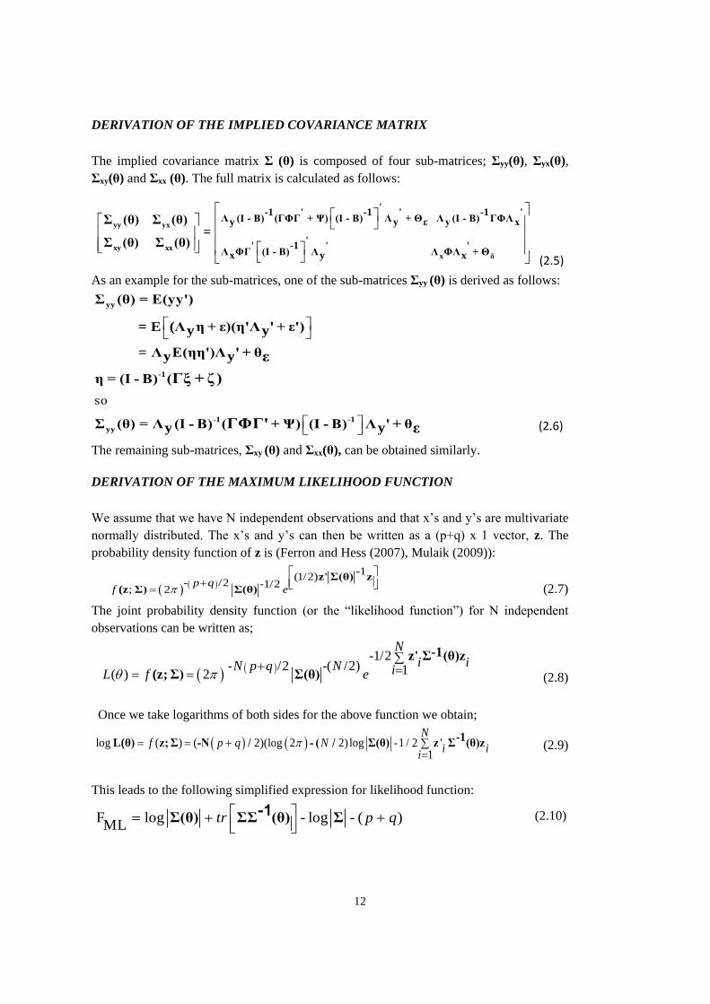
DERIVATION OF THE IMPLIED COVARIANCE MATRIX

The implied covariance matrix Σ (θ) is composed of four sub-matrices; Σyy(θ), Σyx(θ),

Σxy(θ) and Σxx (θ). The full matrix is calculated as follows:

As an example for the sub-matrices, one of the sub-matrices Σyy (θ) is derived as follows:

The remaining sub-matrices, Σxy (θ) and Σxx(θ), can be obtained similarly.

DERIVATION OF THE MAXIMUM LIKELIHOOD FUNCTION

We assume that we have N independent observations and that x’s and y’s are multivariate

normally distributed. The x’s and y’s can then be written as a (p+q) x 1 vector, z. The

probability density function of z is (Ferron and Hess (2007), Mulaik (2009)):

(2.7)

The joint probability density function (or the “likelihood function”) for N independent

observations can be written as;

(2.8)

Once we take logarithms of both sides for the above function we obtain;

(2.9)

This leads to the following simplified expression for likelihood function:

(2.10)

yy

-1

-1 -1

yy

Σ (θ) = E(yy')

= E (Λ η + ε)(η'Λ ' + ε')y y

= Λ E(ηη')Λ ' + θy y

η = (I - B) (

Σ (θ) = Λ (I - B) ( + Ψ) (I - B) Λ ' + θy y

ε

Γξ + ζ )

ΓΦΓ' ε

so

-1(1/2)

- /2 -1/2  ; 2  

p qf e

z' Σ(θ) z

(z Σ) Σ(θ)

-1/2-( /2)- /2 1    ( ) 2

N

i iNN p q iL f e

-1z' Σ (θ)z

(z; Σ) Σ(θ)

 log ( ) ( 2)(log 2 2) log -1 / 2 '1

Nf p q N

i ii

-1  L(θ) z; Σ -N / - ( / Σ(θ) z Σ (θ)z

 F log - log - ( )ML

tr p qΣ(θ) ΣΣ (θ) Σ-1

(2.5)

(2.6)

13

To minimize FML, we can use nonlinear optimization algorithms. Since θ is a function of

ϒ and ψ, the path coefficient vectors, partial derivative of FML with respect to all path

coefficients are taken and the following vector is formed:

(2.11)

Newton- Raphson algorithm works in steps where in each step an adjustment is made over

the results of the former iteration as follows:

(2.12)

The computations are iterated until the implied covariance matrix is the same as the real

observed covariance matrix or until there is no decrease in the difference of implied

covariance matrix and the real covariance matrix.

A full illustration of the algorithm for a numerical example is given by Ferron and Hess

(2007). They give a numerical example for the following model:

Figure 2.4 Ferron and Hess’s (2007) Example Problem

Here, the parameters to be estimated are and ψ. For simplicity, the error variances and

factor loadings are set initially. The steps of solution are as follows:

1. Σ (θ) is computed for the given initial parameter values.

2. Σ(θ) is the matrix of observed covariances which is known initially.

3. FML is calculated with the initial values of Σ and Σ (θ).

4. Partial derivatives of FML are calculated for the first iteration of optimization

algorithm.

5. At the end of 7 iterations, FML =0 and thus the optimal model fit is reached. Σ (θ) is

thus finalized.

FML

FML

γ

ψ

2( 1) ( ) F FML ML-2

i i-1

θ θθθ

14

If the number of parameters is higher and if the sample size is small then estimation

problems can occur. The solution can be simplified and convergence can be ensured by:

Setting some parameter values like the covariate – latent path coefficients to 1

Trying different starting parameter values

Larger sample sizes

Changing the estimation algorithm

Re-screning the data for outliers

Re-scaling variables with variances bigger than the variances of other variables

Revising the model for less number of paths and factor loadings.

IDENTIFICATION OF AN SE MODEL

If the parameters to be estimated are covered by the given data points(the covariances

among the indicator variables) then an SE model is “identified”. If we have enough data

points to yield estimates then the model is said to be “underidentified”. This arises due to

complexity of the models or insufficient sample sizes or inadequate or correlated

measurement error terms. Bollen (1989) and other eminent SEM researchers suggest

remedies for necessary and/or sufficient conditions for identification. Most of these are

not exact rules and shoud be tried for different modeling settings. Our practice is given in

Chapter 5.

Examples of three SE models (Hannemann,1999) are given in Figure 2.5. Each model has

5 measured variables and thus 1/2 (5 × 6) or 15 unique elements in their variance-

covariance matrices. However, the first model is be over-identified by two degrees, since

the number of parameters to be estimated is 13(with 6 covariances, 4 path coefficients and

3error terms), the second is exactly identified (with 6 covariances, 6 path coefficients and

3 error terms) and the last is under-identified (with 6 covariances, 8 path coefficients and 3

error terms). Thus we can say that the first and the second models can be estimated but the

last modelneed to be revised with less number of paths or more data points.

Figure 2.5 Identification of SE Models (Hannemann, 1999)

15

We need to have an identified and not under-identified SE model before we can estimate

its parameters.

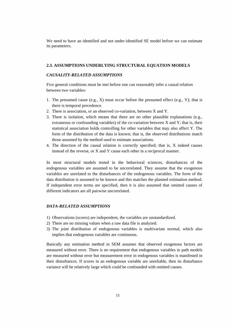
2.3. ASSUMPTIONS UNDERLYING STRUCTURAL EQUATION MODELS

CAUSALITY-RELATED ASSUMPTIONS

Five general conditions must be met before one can reasonably infer a causal relation

between two variables:

1. The presumed cause (e.g., X) must occur before the presumed effect (e.g., Y); that is

there is temporal precedence.

2. There is association, or an observed co-variation, between X and Y.

3. There is isolation, which means that there are no other plausible explanations (e.g.,

extraneous or confounding variables) of the co-variation between X and Y; that is, their

statistical association holds controlling for other variables that may also affect Y. The

form of the distribution of the data is known; that is, the observed distributions match

those assumed by the method used to estimate associations.

4. The direction of the causal relation is correctly specified; that is, X indeed causes

instead of the reverse, or X and Y cause each other in a reciprocal manner.

In most structural models tested in the behavioral sciences, disturbances of the

endogenous variables are assumed to be uncorrelated. They assume that the exogenous

variables are unrelated to the disturbances of the endogenous variables. The form of the

data distribution is assumed to be known and this matches the planned estimation method.

If independent error terms are specified, then it is also assumed that omitted causes of

different indicators are all pairwise uncorrelated.

DATA-RELATED ASSUMPTIONS

1) Observations (scores) are independent, the variables are unstandardized.

2) There are no missing values when a raw data file is analyzed.

3) The joint distribution of endogenous variables is multivariate normal, which also

implies that endogenous variables are continuous.

Basically any estimation method in SEM assumes that observed exogenous factors are

measured without error. There is no requirement that endogenous variables in path models

are measured without error but measurement error in endogenous variables is manifested in

their disturbances. If scores in an endogenous variable are unreliable, then its disturbance

variance will be relatively large which could be confounded with omitted causes.

16

2.4. LONGITUDINAL DATA ANALYSIS WITH STRUCTURAL EQUATION

MODELS

McArdle’s (2009) work is the most recent research which provides a review of longitudinal

structural models. Longitudinal models with two measurement points are depicted in Figure

2.6. The models include one latent variable Y, its intercept factor, Δ, group effects variable,

G and error terms. Longitudinal models with two measurement points, multiple latent

variables and multiple indicators are depicted in Figure 2.7. The models in Figure 2.6 are

further extended to cover multiple measurement points, multiple variables and

autocorrelations as in time series models. The extended models are depicted in Figure 2.7.

Figure 2.6 Longitudinal Models with Two Measurement Points and Group Effects

(McArdle, 2009)

a) Model with Group Codes

b) Two different models

c) Complete and incomplete group models

17

igure 2.7 Multivariate Two Measurement Occasion Structural Models (McArdle, 2009)

a) One latent variable and two periods’ model

b) One latent variable, two periods and change variables’ model

c) Two latent variables and two periods’ model

18

Figure 2.8 Multivariate Multiple Measurement Occasion Structural Models With Time

Series Concepts (McArdle, 2009)

a) One latent variable and four periods’ model

b) Two latent variables and four periods’ model

2.5. STRUCTURAL EQUATION MODELS WITH FORMATIVE LATENT

VARIABLES AND COVARIATES (MIMIC MODELS)

MIMIC (multiple-indicator multiple-cause) models can be used for including time-variant

and time-invariant covariates in structural equation models.

MIMIC modeling is a SEM technique for studying latent variables affected by many

indicators and with affecting indicators. The MIMIC model is actually confirmatory factor

analysis model including covariates. Since a factor analysis model is actually a structural

equation model MIMIC model is a special case of SEM.

The two forms of measurement in structural models are called reflective and formative

measurements. Diamantopulos (1999) gives the following path models to represent two

distinct forms of measurement:

19

Figure 2.9 Reflective and Formative Measurement Models (Diamantopulos, 1999)

In Figure 2.9 (a), reflective measurement latent variable is measured through its

indicators. This is a typical factor loading case in a structural equation model. P represents

a latent variable which is measured through three items in a “scale”. The indicators may or

may not be allowed to correlate and all of them are measured with errors. A high

correlation is not allowed because this violates the assumption of an underlying factor

whose variance is shared by separate indicators. i, i=1,2,3 represent factor loadings. In

Figure 2.9 (b), formative measurement latent variable, P, is caused by variables. i ,

i=1,2,3 represent causal effects. This model is called an “index” and not a “scale”. The

causal variables are allowed to correlate and there is also a disturbance term affecting the

latent variable, P.

Coltman et al. (2008) discuss a framework for selecting formative or reflective latent

variable structures for measuring constructs. They use an international business and a

marketing example to check presence of conditions for using formative constructs. The

checks yield that a formative measurement model is more suitable. They stress that “use

of an incorrect measurement model undermines the content validity of constructs,

misrepresents the structural relationships between them, and ultimately lowers the

usefulness of management theories for business researchers and practitioners”.

MIMIC models can also be used to assess effects of covariates on latent variables through

mediation or through direct effects. Christensen et al. (1998) study effects of age on

anxiety and depression and examined whether age has direct effects on self-report of

individual symptoms independent of its effect on the underlying dimensions of anxiety

and depression. They build the following model:

20

Figure 2.10 Christensen et al.’s (1998) MIMIC model

In the above model, there are two latent variables modeled with reflective structures. Five

covariates affect dependent measurement variables through paths to latent variables and

also through direct effect paths. The covariates represent demographic effects, namely;

age, sex, marital status, educational level and financial status. The researchers tested

whether correlated anxiety and depression factors underlie the symptoms, to assess the

effects of age on the underlying factors, and to see whether age has direct effects on some

of the symptoms. The direct effects of covariates on separate indicators are found to be

significant. These direct covariate- indicator relations are hypothesized before the model is

constructed. The direct effect can be stronger than the indirect effect because indirect

effect assumes that indicator variable only partially accounts for the variation of the latent.

The direct effect, on the other hand, assumes that covariate and indicator variable are

directly correlated and the variation in the indicator variable totally explains the variation

of the covariate variable. The path coefficient is bigger for direct path since there is no

mediation.

21

Christensen et al.’s (1998) study is a MIMIC modeling case with reflective latent variable

structures and covariates.

Pynnonnen (2010) formulates the following path model of a MIMIC structural equation

model. There is one latent variable with three indicators and three causal variables. Thus

this is a latent variable with both reflective and formative structures.

Figure 2.11 A MIMIC Model (Pynnonnen, 2010)

ALGEBRA OF MIMIC MODELS

For a MIMIC model with a single latent variable (), one indicator variable (y) and one

causal variable (x) the path model and structural equations are as follows (Bollen,1989):

Figure 2.12 A MIMIC Model’s Path Diagram

x

y

(2.13)

Here ε represents measurement error associated with the indicator variable. The causal

variables (or covariates) are assumed to be free of measurement error. These correspond to

general questions or general questions with no scaled answers in questionnaires. A typical

example is “age of respondent”. Here an exact answer is assumed.

MIMIC MODELS AS A MODELING APPROACH FOR MULTI-GROUP ANALYSES

In the literature, basically two types of structural equation models are presented to analyze

the difference in means: multiple-groups models and multiple-indicator, multiple-cause

x y

22

models. The multiple-groups models may be conceptualized as analogous to ANOVA

models, whereas MIMIC models may be thought to be analogous to regression models. In

multiple group models the comparison between two groups differing by an effect variable

can be analyzed (Green and Marilyn, 2006).

We may want to test whether the factor models are similar between different groups. For

example are the indicators measuring same underlying factors in different groups have

similar values or are the similar indicators loaded similarly on common factors with the

same coefficients. These are achieved by building the same structural model separately for

different groups. For example, comparison can be made on the basis of gender, age or

similar outer effect variables. An example model is given below. Boys and girls are

assessed for three latent variables with nine indicators. There are two identical models

differing on the source of data. First set is from boys and the second set is from girls.

Figure 2.13 A MIMIC Model with three latent variables and nine- indicator Variables

(Pynnonnen, 2010)

The algebraic representations of the models do not differ. We do not add a separate

variable for group effects. The analysis results are compared. The sets of hypotheses

tested are:

1. Factor patterns are the same

2. Error variances are the same

3. Factor covariances are the same

For a SE model with a single set of data we test the following hypotheses:

1. Actual covariance matrices are the same as estimate covariance matrices in the

hypothesized path model (structural model).

2. Actual factor loadings are the same as estimated factor loadings (measurement model)

23

2.6. LITERATURE SURVEY ON CUSTOMER LOYALTY MODELS

2.6.1. DEFINITIONS OF LOYALTY AND SATISFACTION

There is not a well-established and clear definition of customer loyalty in marketing

literature. Kotler’s (2006) definition can be given as a concise definition for the

“customer satisfaction” framework. Kotler states that; “customer satisfaction measures

how well a customer’s expectations are met”.

For customer loyalty, there are three distinctive definitions (Bowen and Chen, 2001)

which are:

– Attitudinal, that is an attachment to a product, service or an organization,

– Behavioral, that is consistent, repeated purchase behavior as an indicator of loyalty.

However, repeated purchases are not always the result of a psychological commitment

toward the brand (Te Peci, 1999),

– Composite loyalty, combining both attitudinal and behavioral loyalty aspects and

measuring loyalty by customers' product preferences, propensity of brand-switching,

frequency of purchase, recency of purchase and total amount of purchase (Pritchard

and Howard, 1997; Hunter, 1998; Wong et al., 1999).

Within the framework of our research, we will use the “composite” definition for

customer loyalty. Thus, customer loyalty can be defined as the combination of customer’s

attachment attitudes toward the product/service or organization/brand and the purchase

frequency of the product/service. We use a composite of attitudinal and behavioral loyalty

scale items in our questionnaire.

The two major arguments for customer satisfaction-customer loyalty relations are stated

as: (Hallowell, 1996):

1. Customer satisfaction influences customer loyalty. Customer loyalty, then, affects

profitability (Anderson and Fornell, 2000).

2. Customer loyalty can be defined as either (Bowen and Chen, 2001).

Bowen and Chen (2001) point to the concept of “extreme satisfaction” as the major

indicator of loyalty. Sivadas and Baker–Prewitt (2000) state that, “satisfaction itself will

not translate into loyalty”. Many other authors indicate cause-effect relation between

customer satisfaction and future purchase behavior (La Barbera and Mazursky, 1983).

Kwang et al. (2007) refer to various studies on relationships between service performance

to the customer satisfaction and customer loyalty in various service sectors as hotels,

tourism, medical services, telecommunication services, banking and internet services.

Most of these show causal relationships between service performance, customer

satisfaction and customer loyalty.

24

There is abundant literature pertaining to relationships between customer satisfaction,

customer loyalty and profitability. Kotler (2000) defines satisfaction as “a person’s

feelings of pleasure or disappointment after comparing a product’s perceived performance

(or outcome) in relation to his or her expectations”. Satisfaction can be associated with

feelings of acceptance, happiness, relief, excitement, and delight. Dissatisfied consumers

can decide to (Singh, 2006):

– Discontinue purchasing the good or service,

– Complain to the company or to a third party and perhaps return the item or

– Have negative word-of-mouth communication.

Satisfied customers can, on the other hand have repurchase intentions, positive word-of-

mouth and positive collaboration (La Barbera and Mazursky, 1983).

The original interest in customer satisfaction research is on customer's experience with a

product episode or service encounter (Yi, 1990; Anderson et al., 1993). More recent

studies have focused on cumulative satisfaction. Cumulative satisfaction defines

satisfaction as customer's overall experience to date with a product or service provider.

This approach to satisfaction provides a more direct and comprehensive measure of a

customer's consumption utility, subsequent behaviors and economic performance (Fornell

et al., 1996). Customer Satisfaction Index studies are formulated using the “cumulative

satisfaction” concept.

Satisfaction with a product occurs after a consumption experience. Customer expectations,

on the other hand, form before the first consumption experience and they mature during

consumption process. Thus we need to consider all factors which directly and indirectly

affect customer satisfaction for pre-purchase, purchase and post-purchase periods.

Marketing literature refers to various forms of “quality” related to consumers’ satisfaction

and loyalty formation.

“Quality of goods” should be considered as additional dimension of “customer

satisfaction” variable. According to Garvin’s (1987) definition, there are eight distinct

dimensions of product quality. These are:

- Performance: The primary operating characteristics of a product

- Features: the secondary characteristics of a product, which supplements “performance”

- Reliability: The probability that the product will fail in a period of time

- Conformance: A product’s conformance to pre-established standards

- Durability: The expected period of use of a product before it deteriorates or completely

fails

- Serviceability: Speed, courtesy, competence and ease of repair

- Aesthetics: The look, feel, taste, smell and sound of a product

- Perceived Quality: The impact of brand name, company, image and advertising.

25

2.6.2. IMPORTANCE OF LOYALTY IN CUSTOMER RELATIONSHIP

MANAGEMENT

Customer relationship management (CRM) programs use existing customers’ information

to improve companies’ long-term relationships and profitability (Couldwell, 1999; Glazer,

1997, as cited in Payne and Frow, 2005). Long-term profitability can thus be increased

through customer communication strategies to improve customer acquisition, retention

and also customer loyalty. On the other hand, it is long known that acquiring new

customers or re-gaining lost customers are much more costly than achieving and

improving existing customers’ loyalties. Reichheld and Sasser (1990) estimate that a 5%

increase in customer loyalty can produce profit increases from 25% to 85%. In other

words, it is more rewarding to elevate customer loyalty than acquiring or retention

programs. Thus loyalty is an indispensable component of CRM in modern organizations.

2.6.3. LOYALTY MODELS IN LITERATURE

A number of loyalty models are studied in literature. Most of these use structural equation

modeling approach to study antecedents and consequences of loyalty. Some use SEM to

formulate customer satisfaction indices for selected goods or services. These are presented

and detailed in this section to provide the conceptual background for our research model

which is presented in Chapter 3.

Fornell et al. (1996) suggest a comprehensive path model for the antecedents and

consequences of overall customer satisfaction and customer loyalty. It is the first large

scale model in loyalty modeling context.

Figure 2.14 Customer Satisfaction- Customer Loyalty Path Model (Fornell, 1996)

Yu et al. (2005) use Fornell et al.’s model to measure customer satisfaction and customer

loyalty for Lexus Cars in Taiwan. This is a comprehensive structural equation modeling

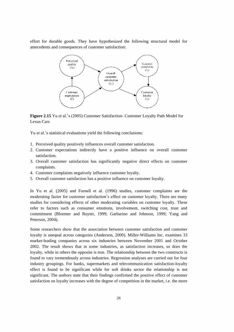
26

effort for durable goods. They have hypothesized the following structural model for

antecedents and consequences of customer satisfaction:

Figure 2.15 Yu et al.’s (2005) Customer Satisfaction- Customer Loyalty Path Model for

Lexus Cars

Yu et al.’s statistical evaluations yield the following conclusions:

1. Perceived quality positively influences overall customer satisfaction.

2. Customer expectations indirectly have a positive influence on overall customer

satisfaction.

3. Overall customer satisfaction has significantly negative direct effects on customer

complaints.

4. Customer complaints negatively influence customer loyalty.

5. Overall customer satisfaction has a positive influence on customer loyalty.

In Yu et al. (2005) and Fornell et al. (1996) studies, customer complaints are the

moderating factor for customer satisfaction’s effect on customer loyalty. There are many

studies for considering effects of other moderating variables on customer loyalty. These

refer to factors such as consumer emotions, involvement, switching cost, trust and

commitment (Bloemer and Ruyter, 1999; Garbarino and Johnson, 1999; Yang and

Peterson, 2004).

Some researchers show that the association between customer satisfaction and customer

loyalty is unequal across categories (Anderson, 2000). Miller-Williams Inc. examines 33

market-leading companies across six industries between November 2001 and October

2002. The result shows that in some industries, as satisfaction increases, so does the

loyalty, while in others the opposite is true. The relationship between the two constructs is

found to vary tremendously across industries. Regression analyses are carried out for four

industry groupings. For banks, supermarkets and telecommunication satisfaction-loyalty

effect is found to be significant while for soft drinks sector the relationship is not

significant. The authors state that their findings confirmed the positive effect of customer

satisfaction on loyalty increases with the degree of competition in the market, i.e. the more

27

competitive a market is, the more sensitive changes in loyalty are to changes in customer

satisfaction (Lars et al., 2000).

Lars et al. (2000) use the basic European Customer Satisfaction Index (ECSI) model to

define antecedents of Customer Loyalty. The basic ECSI model is given in Figure 2.16.

The hypothesized model is tested for telecommunication industries, four

telecommunication industries (fixed net, mobile phones, the Internet and cable television),

retail banks, supermarkets, the soft drink industry and fast food restaurants. Their findings

can be listed as follows:

Figure 2.16 European Customer Satisfaction Index Model (Lars et al., 2000)

Figure 2.17 ECSI Model Extended to Include Trust and Communication (Ball et al. 2004)

28

1. Customer satisfaction has a positive effect on loyalty.

2. Low price companies have larger loyalty than their expectations from customer

satisfaction.

3. Companies with a lot of branding efforts have high customer satisfaction but they do

not have a correspondingly high loyalty.

4. Customer complaints negatively influence customer loyalty.

5. Overall customer satisfaction has a positive influence on Customer Loyalty.

Ball et al. (2004) extends the ECSI model to include communication and trust. They show

that customer loyalty can to a substantial extent be explained by communications and trust

as well as the other variables. Communication is a latent variable measured through:

- Ease and satisfaction of relationship with the service provider

- Keeping informed about new products/services

- Personal services /advice

- Clearness and transparency of information

Trust is measured with two dimensions; performance/credibility trust and benevolence

trust. Consumers evaluate service–sellers based on the performance of the services

purchased, credibility of the company and also with benevolence and integrity of the

service company.

Ball et al. (2004) hypothesize antecedents of loyalty as stated in their conceptual model.

Their findings reveal the following results:

- For the narrower ECSI model, loyalty is primarily explained by satisfaction, quality and

image,

- For the extended ECSI model, loyalty is explained primarily by satisfaction and

communication.

Türkyılmaz and Özkan (2007) build a comprehensive structural model of customer

satisfaction for mobile phones in Turkey based on the customer satisfaction indices (CSIs)

of developed countries. Their model is given in Figure 2.18. The definitions of the latent

variables in the hypothesized model are as follows:

1. “Image” construct evaluates the underlying image of the company. Image refers to the

brand name and the kind of associations customers get from the product/company.

2. “Customer Expectations” are the results of prior experience with the company's

products. This variable depends on customer expectations for overall quality, for

product and service quality, and for fulfillment of personal needs.

3. Perceived Quality” is the consumers’ (so called “served market’s”) evaluation of recent

consumption experience. This variable evaluates customization and reliability of a

given product or service.

29

Figure 2.18 Türkyılmaz and Özkan (2007)’s Customer Satisfaction Loyalty Model for

Turkish Mobile Phone Industry

4. Perceived Value” is the perceived level of product quality relative to the price paid by

customers. This latent variable is defined as “the rating of the price paid for the quality

perceived and a rating of the quality perceived for the price paid”.

5. “Customer Satisfaction” is defined as the latent variable which shows how much

customers are satisfied, and how well their expectations are met. This latent variable is

elaborated as the “overall satisfaction level of customers, fulfillment of their

expectations, and company's performance versus the ideal provider.

6. “Customer Loyalty” is measured by repurchase intention, price tolerance and intention

to recommend products or services to others.

Türkyılmaz and Özkan’s (2007) statistical evaluations yield the following conclusions:

1. Satisfaction is mostly affected by perceived value.

2. Perceived quality and image also have considerable effects on satisfaction.

3. Customer satisfaction and company image have positive and significant effects on

customer loyalty.

4. Customer satisfaction is found to be the most important factor for improving customer

loyalty.

Lin and Wang (2006) study antecedents of customer loyalty in mobile commerce context.

They find that trust is an important determinant of customer satisfaction and loyalty.

30

Andreassen and Lindestad (1998) examine effects of corporate image or simply image on

quality, customer satisfaction and loyalty for customers at different expertise levels for

infrequent purchase and complex services. Their conceptual model is as follows:

Figure 2.19 Habits as an Antecedent of Loyalty (Andreassen and Lindestad, 1998)

The ‘+’ and ‘-’ signs on the picture denote the positive or negative causality effects. A

positive causality shows an increase in the effect variable caused by an increase in the

causal variable. Similarly, a ‘-’ sign shows a decrease in the effect variable cause by an

increase in the causal variable.

They concluded that corporate image plays more important role for customer loyalty than

customer satisfaction. They define trust dependent on image. Image in mobile commerce

context is assumed to have integrity, benevolence, competence and predictability.

Habitual preferences or “habit” is found to have a significant effect on customer loyalty.

They state that once customers begin using mobile service and become familiar with it

they may be inclined to continue, if it becomes a habit.

Many researchers have studied effects of word-of-mouth as a consequence of satisfaction

and as an antecedent of loyalty. Zeithaml (2000) finds out that loyal customers have

higher retention rates, commit a higher share of their spending and more likely to

recommend others to become customers of the firm. Mazzarol et al. (2008) emphasize that

word-of-mouth is the key to competitive advantage in market place. Türkyılmaz and

Özkan (2007) refer to word-of-mouth as “recommend to others” which in turn is defined

as an indicator of customer loyalty. Roy et al. (2009) examine the effects of customer

loyalty on word-of-mouth behaviors for online retail markets. They classify four distinct

loyalty consumer attitudes as follows:

Cognitive loyalty: The loyalty state based on brand beliefs

Affective loyalty: Level of favorable attitudes and like the customer displays towards

the brand

Conative loyalty: The development of behavioral intention to continue to buy the

brand.

Action loyalty: The stage where behavioral intentions are converted into actions. This

defines the “true loyalty”.

31

They hypothesize the model in Figure 2.20, based on the above four distinct loyalty

attitudes. Statistical analyses yield that conative and affective loyalty states relatively

seem to prompt the word-of-mouth behavior more than the action loyalty attitudes.

Cognitive loyalty is found to have no significant effect on online word-of-mouth attitudes.

Word-of-mouth attitudes or customers’ potential attitudes for recommendations to other

consumers can be similarly integrated into our conceptual model.

La Barbera and Mazursky (1983) stress that satisfied customers have repurchase

intentions, positive word-of-mouth and positive collaboration.

Figure 2.20 Effects of Different Loyalty Attitudes on Online Word-of-Mouth Behaviors

of Customers (Roy et al., 2009)

Chiou (2004) states that customer satisfaction, although being important, cannot explain

all the variance of customer loyalty. He further added that loyalty may become

independent of satisfaction and sometimes ‘temporary reversals’ of satisfaction may not

be accounted for long term loyalty intention. In our context, experts of two leading

durable goods manufacturers (Pakkan (2010) and Akgözlü (2010)) suggest that loyalty is a

consequence and time-based natural result of customer satisfaction. In survey and

modeling phases, we will test existence of latent variables. Testing isolated loyalty-

satisfaction link will yield the importance of the assumed causality relationship.

Satisfied customers have a high intention to buy the same product, and loyal customers

must be satisfied with the product. Customer satisfaction certainly is one of the primary

ingredients that create customer loyalty although it is not equal to loyalty (Wu and Shao,

2003 as cited in Wang, 2007). Satisfied customers may not always become loyal. The

phenomenon of high satisfaction and low loyalty is called “satisfaction traps” (Wang,

2007; Jones and Sasser, 1995).

Jones and Sasser (1995) state the concept of “false loyalty” to refer to satisfied but ready-

to-switch customers. They stress that even in low competitive markets “providing

customers with outstanding value” is the key for satisfied customer being also loyal. Their

important finding is that even in less intense competition markets customer stay “rock

solid loyal” if they are completely satisfied. More than half of the satisfied customers are

found to “defect” (switch to another brand or stop consumption) eventually.

32

Zeithaml et al. (1988) examine time-related aspects of service consumption. The “gaps”

indicate the differences between service quality/delivery realizations of the service

provider and the service quality/ delivery expectations of the consumers. These gaps are

illustrated in Figure 2.21. The gaps model is further extended to cover antecedents of

customer satisfaction (see Figure 2.22).

Tse et al. (1990) suggest the following propositions for evaluating consumers’ satisfaction

process:

1. The level of post-consumption stress experienced by a consumer is a function of the

primary effect of the consumption experience and the perceived difference between the

consumption experience and its pre- experience standards.

2. The more experience a consumer has with the product the more likely he or she would

attribute any product performance discrepancy to the product rather than to himself or

herself.

3. A product's subjective meaning will change as consumers change their socioeconomic

status.

Figure 2.21 The “Gaps” Service Quality Model (Zeithaml, 1988)

4. A consumer's perceived product performance is the most influential determinant in his

or her satisfaction process.

5. Consumers adjust their expectations regarding a product's performance as the product

deteriorates over time.

6. Consumption situation exerts significant influences on consumers' satisfaction

evaluation through their influence on a product's instrumental and/or expressive

factors.

7. The more a consumer perceives the consumption situation similar to previous

consumption situations the more influential the previous consumption would be in the

satisfaction process.

33

Corporate image is perceived as a function of purchasing/consumption experience over

time (Andreassen and Lindestad, 1998). Aaker and Keller (1990) defines “corporate

image” as “perceptions of an organization reflected in the associations held in consumer

memory”.

Figure 2.22 Extended “Gaps” Service Quality Model (Zeithaml et al., 1988)

Bontis et al. (2007) study mediating effects of organizational reputation on service

recommendation and customer loyalty. Their findings reveal that reputation is a

consequence of satisfaction and is an antecedent of loyalty. They summarize this as the

partially mediating effect of reputation on loyalty. In our conceptual model, reputation-

satisfaction link will be investigated again in an isolated factor and isolated link context.

We will use “reputation” and “corporate image” terms interchangeably. Walsh et al.

(2009) define customer-based reputation as “the customer’s overall evaluation of a firm

based on his or her reactions to the firm’s goods, services, communication activities,

interactions with the firm and/ or its representatives or constituencies (such as employees,

management or other customer) and/ or known corporate activities.”

There are alternative definitions of reputation in the literature. Walsh et al. (2009)

hypothesize, test and confirm the following relationships for a sample of German energy

consumers:

1. Customer satisfaction is a positive antecedent of reputation

The association is confirmed.

2. Trust is a positive antecedent of reputation

The association is confirmed.

3. Reputation is a positive antecedent of customer loyalty.

The association is confirmed.

34

4. Reputation is a positive antecedent of customers’ positive word- of- mouth

The association is confirmed.

Caruana et al.(2000) defines perceived quality as “the result of the evaluation they make

of what is expected and what is experienced.” This definition leads to ideas about

formulating a scale for perceived quality construct. The scale should measure expectancies

and experience at the same time. Presence of experience indicates the need for time-based

formulation as well. Perceived quality is a time consequence of product/service utilization.

Thus it is included in the latter (closer-to-present) measurement occasions in the

measurement model.

In customer satisfaction research, word-of-mouth refers to positive product / service

recommendation attitudes of customers. Zeithaml (2000) and Dick and Basu (1994) study

word-of-mouth-loyalty relationships in various contexts. Their findings point to the

common fact that loyal customers are more likely to develop ‘positive recommendation’

attitudes.

Bontis et al. (2007) study the mediating effect of reputation between satisfaction and

word-of-mouth. Reputation is found to have a direct positive mediating effect between

satisfaction and recommendation. There are a number of alternative definitions of

switching behaviors and affecting factors in literature. These pertain to service industries.

This makes sense because only for service industries and only for quick–consumption

goods consumers can make comparisons and can want to change their service providers in

the short-run. “Insensitivity to competitive offerings” reflects a high degree of customer

allegiance in spite of situational influences and marketing influences like campaigns or

promotions. For durable goods, switching behavior is mostly observed for institutional

customers. This research aims to measure the nature of similar renewal/ first-time

purchase attitudes for individual customers.

Lin and Wang (2006) study antecedents of customer loyalty in mobile commerce context.

They find that trust is an important determinant of customer satisfaction and loyalty.

2.7. SCALING AND VALIDATION

Our research aims to measure consumers’ perceptions towards use of air-conditioners.

Thus we aim to collect data on these perceptions. This can be done through a structured

survey consisting of groups of questions measuring groups of perceptions. Each group

corresponds to a construct (latent variable) in a structural equation model and each

question refers to an item.

Thus we need a measurement tool containing a set of suitable questions to collect data

from a targeted sample.

The formal definitions for scaling can be given as follows (Hardesty and Bearden, 2004;

Alpar, 2010):

35

A “measurement tool” or an “instrument” is a test or a collection of suitable questions to

collect data from a sample.

A “survey” is commonly used measurement tool which consists of ordered questions

with multiple-choice or open-ended answer questions.

A “sample” is a representative part of a target population. “Sample data” refers to the

answers of respondents in the selected sample.

A “scale” is a group of questions aiming to measure the same latent variable.

An “item” is a question in a scale.

A “questionnaire” is a combination of scales selected by the researcher.

2.7.1. LITERATURE REVIEW ON SCALES IN OUR RESEARCH COMPANY

IMAGE (REPUTATION) CONSTRUCT

Selnes (1993) studies effects of product performance on brand reputation, customer

satisfaction and customer loyalty. He emphasizes that reputation is a key factor affecting

customer loyalty. He emphasizes that a key function of a brand is that “it facilitates choice

when intrinsic cues or attributes are difficult or impossible to employ”. He refers to Aaker

and Aaker and Keller’s (1990) definition of brand reputation. They define brand

reputation as “a perception of quality associated with the name”. Selnes (1993) collect

data from four companies. These are an insurance company, a telephone services

company, a business college and a salmon feed supplier company.

The causal path from brand reputation to loyalty is found significant for all four industries.

Bontis et al. (2007) study the mediating effect of organizational reputation on service

recommendation and customer loyalty for a North American Bank. They develop an

extended model which hypothesized a causal relation between corporate image and

customer loyalty. They include satisfaction loyalty, satisfaction–reputation–loyalty and

satisfaction– recommendation causality links. Their findings reveal that reputation

partially mediates satisfaction–loyalty relationship and also satisfaction–recommendation

relationship. They also provide a review of reputation measurement conventions in the

literature. They define reputation as a“global valuation”. Thus they adapt a multiple-

stakeholder approach in defining reputation. They measure reputation by a single indicator

question asked to customers.

Walsh et al. (2009) provide a comprehensive review of corporate reputation literature.

They generalize the definition as “the customer’s overall evaluation of a firm based on his

/ her reactions to the firm’s good, services, communication activities, interactions with the

firm and / or its representatives or constituencies (such as employees, management or

other customers) and / or corporate activities”. We will use this latter definition.

Walsh et al. (2009) use a 15-item measurement of this latent variable. The measurement

covers customer / employer / financial strength and reliability product and service quality

36

/social and environmental responsibility evaluation aspects. This is a long scale. A

shortened version of the list is as follows:

Customer Orientation (Cronbach = 0.92):

The company treats its customers in a fair manner.

The company’s employees are concerned about customer needs.

The company’s employees set great store by a courteous customer treatment.

The company takes customer rights seriously.

Part of Good Leadership Sub-scale (Cronbach = 0.89):

(The company) Has excellent leadership.

Part of Product and Service Quality Sub-scale (Cronbach is not calculated for these

items but the scale is used for regression of loyalty over the indicators, an overall

confirmatory factor analysis is undertaken to assess measurement quality):

(The company) offers high quality products and services.

(The company) is a strong and reliable.

(This is part of Social and Environmental Responsibility Sub-scale (Cronbach is not

calculated for these items but the scale is used for regression of loyalty over the

indicators):

(The company) is an environmentally responsible company.

COMMUNICATIONS CONSTRUCT

The European Customer Satisfaction Index (ECSI) model is an extension of American

Customer Satisfaction Index (ACSI) model for assessing customer satisfaction and its

antecedents and consequences. Ball et al. (2004) include two new latent variables into

ESCI model. These are communication and trust. The authors confirm the

communication-loyalty and trust-loyalty links. They define the following items to assess

this construct:

I have an easy and satisfactory relationship with the company

The bank keeps me constantly informed of new products and services that could be in

my interest

Personal service and advice of my bank

Clearness and transparency of information provided by the bank

The above items are developed for business-to-consumer context for repeated purchases /

frequent transaction services (like banking). The above items are not tested for reliability

37

but are tested for their overall R2 values and their inter-item reliabilities for the special

case studied in the research paper.

In our case a good is bought and then after installation frequent transactions can only

occur in complaint–handling situations or with similar occurrences, at a low frequency.

PERCEIVED QUALITY CONSTRUCT

In the research setting, we have both product and service quality aspects. By “services” we

mean all the advice, installation, complaint-handling and similar services related to the

product purchased. To define perceived quality, we make use of service quality, quality

and related topics. Yieh et al. (2007) provide the most comprehensive framework. Their

novice contribution is the breakdown of quality concept into two dimensions as:

Service quality

Product quality

They base their service quality findings on service quality concept of Parasuraman et al.

(1988) Parasuraman et al.’s (1988) original index contains five categories:

Tangibles

Reliability

Responsiveness

Assurance

Empathy

Yieh et al. (2007) re-group the five categories of Parasuraman’s quality index into three

categories as follows:

Tangibles

Interaction

Empathy

Brucks et al. (2000) define six items to measure perceived quality of durable goods for

customers who purchase only after assessing the quality of the product:

Ease of use

Versatility

Durability

Serviceability

Performance

Prestige

Caruana and Ewing (2010) hypothesize a model for loyalty of websites or online loyalty.

They defined quality with four dimensions with reference to Wolfinbarger and Gilly's

38

(2003) research; fulfillment / reliability, customer service, website design and

privacy/security.

For our research problem, we define “perceived quality” as: “Customization and reliability

of the given product together with its pre-consumption and post-consumption service

quality characteristics”. A list of relevant items for our setting can be given as follows:

Overall evaluation of the good’s quality experience (item borrowed from Yieh et al.,

2007)

Fulfillment and reliability (item borrowed from Wolfinbarger and Gilly, 2003)

Responsiveness (item borrowed from Parasuraman et al.,1988)

Ease of use (item borrowed from Brucks et al., 2000)

Durability (item borrowed from Brucks et al., 2000)

Serviceability (item borrowed from Brucks et al., 2000)

Performance (item borrowed from Brucks et al., 2000)

Some of the above items are not tested for their overall measurement quality. Brucks et al.

(2000) test the items for significance of each item on customer loyalty. The authors of do

not conduct a construct validity study.

PERCEIVED VALUE CONSTRUCT

Zaim et al. (2010) define perceived value as the level of product quality relative to the

price paid by the customers. They analyze customer satisfaction with Türk Telekom

company’s services and also for Turkish mobile phone users. They use Fornell’s (1996)

scale to measure the construct as follows:

1. Price versus performance

2. Performance versus price

A similar conceptualization is made by Yu et al. (2005). They examine customer

satisfaction- customer loyalty affecting factors for Lexus cars in Taiwan. They again use

Fornell’s (1996) measurement scales.

Using only price as the value perception criterion may be too broad for our case. Durable

goods and especially necessity durable goods users can involve price and other factors to

make an overall assessment of the value of the good and related services.

Kuo et al. (2009) study the relationships among service quality, perceived value, customer

satisfaction, and post-purchase intention in mobile value-added services. They made a

comprehensive conceptualization of the Perceived Value construct as “perceived value is the

evaluation of the benefits of a product or a service by customers based on their advance

sacrifices and ex-post perceived performance when they use mobile value-added services”.

This definition can be adapted to our research setting as “the overall evaluation of the benefits

39

of products / services based on consumers’ utilization of the products and considering the

product’s performance”. Their adapted scale to measure this construct as follows:

I feel I am getting good services for a reasonable price (item borrowed from Cronin et

al., 2000)

Using the services of this company is worth sacrificing some time and efforts (item

borrowed from Tung, 2004)

Compared with other manufacturing companies, it is wise to choose this company

(item borrowed from Wang et al., 2007)

CUSTOMER SATISFACTION CONSTRUCT

Zaim et al. (2010) use ASCI scales in their measurement model for customer satisfaction

and loyalty for Turkish mobile phone users. Their relevant measurement items are:

How much is a customer satisfied?

Level of fulfillment of expectations?

Product’s performance versus an ideal product in customer’s (your) mind?

Zaim et al. (2010) test the above items for convergent and discriminant validities. The

results are satisfactory.

Brown et al. (2005) develop a seven-item scale to measure a customer’s level of

satisfaction with several aspects of a brand of car. Reliability and validity values are

satisfactory. Their relevant items for assessing quality of a product are:

(How satisfied are you with)

Appearance

Power

Features

Quality

CUSTOMER EXPECTATIONS CONSTRUCT

American Customer Satisfaction Index (ACSI) model uses a “pre-purchase” evaluation of

customer feelings to assess this latent variable. This also conforms to our hypothesized

model. “Expectations” is a pre-purchase construct. In the long-run or once the product is

used for some time, realized satisfaction/loyalty succeeds expectations and we need not

measure expectations in post-purchase phase again. The two items to measure the

construct are as follows:

How well does the product fit the customer’s personal requirements? (pre-purchase)

How often things would go wrong? (pre-purchase)

40

COMMITMENT CONSTRUCT

Matos et al. (2009) review and test different service loyalty studies and they test

competing models for mediating, moderating and predecessor roles of switching costs on

satisfaction and loyalty for retail banking industry.

Fullerton (2011) hypothesizes the following model for antecedents and consequences of

satisfaction in business-to-business relationships.

Figure 2.23 Commitment Behavior and Advocacy Intentions (Fullerton, 2011)

Commitment is an attitude towards the act of maintaining a relationship with a partner. It

is studied in three dimensions as follows:

Affective commitment is feeling of positive attachment and enjoying the business

relationship,

Continuance commitment is the extent to which a customer feels bound to a relational

partner. It has a more comprehensive definition including all side effects, switching

costs, etc. Continuance commitment is the psychological state that is brought forward

when consumers face significant economic or psychological switching costs and as a

result perceive few alternatives outside the existing relations,

Normative commitment is the extent to which a customer feels obligated to do business

with a partner. When an individual is normatively committed to an organization they

feel that continuing to be involved with that organization is the right thing to do (Allen

and Meyer, 1990). Normative commitment can be built through a concept of

reciprocity as a force of influence in an exchange situation.

Affective and normative commitments are more important for individual consumers while

continuance commitment may become dominant for business (organizational) customers.

We will use the following scale to assess commitment construct. All items are borrowed from

Fullerton (2011). They are all tested for reliability and validity but for service sectors.

It would be very hard for me to switch away from X right now even if I wanted to

It would be too costly for me to switch from the X right now

I feel obligated to continue to doing business with C

If I got a better offer from another X, I would not think it right to switch away from my X.

41

TRUST CONSTRUCT

Ball et al. (2004) develop an extension of European Customer Satisfaction Index (ECSI)

model to analyze customer satisfaction – customer loyalty relationships for banking

sector. They include communications and trust variables into ECSI basic model. They

define the following items to assess trust:

Overall, I have complete trust in my bank.

When the bank suggests that I buy a new product it is because it is best for the

situation.

The bank treats me in an honest way in every transaction.

Yieh et al. (2007) study the antecedents and consequences of satisfaction and trust for

automobile service and repair centers operated by Taiwan’s major car manufacturers.

They define the following items to measure trust:

The service personnel have the professional knowledge and skill to ensure that my car

is in good repair.

I can trust the employees of the service center to consider my best interest.

CUSTOMER LOYALTY CONSTRUCT

There is an abundant number of loyalty definitions in the literature. Sramek et al. (2008)

give a list of 24 different definitions. Among those, the most suitable ones for our research

problem can be given as follows.

1. Loyalty is a “long-term commitment to re-purchase involving both repeated patronage

and a favorable attitude” (Dick and Basu, 1994).

2. Loyalty expresses “an intended behavior related to a product or a service, including the

likelihood of future purchases or renewal of service contracts, or conversely, how

likely it is that the customer will switch to another brand or service provider” (Selnes,

1993).

Fornell et al. (1996) use a price-related definition for customer loyalty. They use a three-

item scale to assess loyalty. Two of the items measure price-tolerance and one asks about

re-purchase intention. This is a very restrictive evaluation for our research problem.

Kuo et al. (2009) study the relationships between relationships among service quality,

perceived value, customer satisfaction, and post-purchase intention in mobile value-added

services. They use a more comprehensive three-item scale to evaluate customers’ loyalty

to the service-provider company.

Selnes (1993) uses the following items to assess loyalty construct:

How likely is that you will buy products/services from the company in the future?

If another person asked your advice, how likely is that you will recommend this company?

42

INSENSITIVITY TO COMPETITIVE OFFERINGS CONSTRUCT

There are a number of alternative definitions of switching behaviors and affecting factors

in literature. These pertain to service industries. This makes sense because only for service

industries and only for quick–consumption services consumers can make comparisons and

can want to change their service providers in the short-run. In our research setting, there is

an “infrequent purchase” setting where a good is bought and used for long years. These

years may cover long-term contracts, renewal of contracts and similar “continuing

relationship” cases. We need to talk about evaluation of alternatives instead of “switching

decisions”.

Insensitivity to competitive offerings reflects a high degree of customer allegiance in spite

of situational influences and marketing influences (like campaigns or promotions) (Oliver,

1999). Scheer et al. (2010) use this definition and develop a new scale to study industrial

customers’ loyalty. We use their definition and their scale for our research setting. Their

approach is a more comprehensive view of “switching tendencies” for both individual and

also organizational customers. Their scale items are as follows:

If a competing supplier would reduce its price by a small percentage, we would

switch and buy this good from that supplier (reverse-scored).

Any small change in this supplier’s or a competing supplier’s product offerings could

result in our firm changing our source for this product (reverse-scored).

Right now, we buy this good from this supplier, but that could change very quickly

(reverse-scored).

The reliability and validity of all items are tested and the scale proved to be satisfactory.

2.7.2. VALIDATION OF SCALES

BASIC DEFINITIONS OF LIKERT SCALES

Likert scale is a commonly used psychometric scale in research involving questionnaires. The

scale is named after psychologist Rensis Likert (Likert, 1932). Respondents are expected to

specify their level of agreement or disagreement on a series of related statements with

symmetric (equidistant) responses. Thus Likert- scaled questions differ from multiple-choice,

open-ended or true/ false questions. “Midpoint” is defined as the neutral “undecided” choice

marker in a symmetric scale. It divides the response categories into two intervals; first interval

is the set of choices towards full disagreement or fully negative opinion and second interval is

the set of choices towards full agreement or fully positive opinion. Midpoint may or may not

exist in these scales (Albaum, 1997; Netemeyer et al.; 2003).

VALIDITY OF SCALES

There are a number of different validity definitions in literature. It is argued that “validity”

is an evolving concept. A common statistical definition can be given as “the degree to

43

which a test, scale or assessment measures what it is supposed to measure” (Garrett-

Meyer, 2006). This is still a broad and vague definition. A common classification is as

follows (Alpar, 2010):

Content Validity: refers to the ability of a measurement instrument’s to cover all

related items in the target research domain. American Psychological Association gives

a clear definition as; “Content validity refers to the degree to which the content of the

items reflects the content domain of interest”. With this classical definition we can say

that an instrument (a questionnaire in our context) is “content-valid” if each question

reflects the intended latent variable. This can only be assessed through suitable

references as expert opinions and literature surveys.

Construct Validity: refers to the measures associated with their constructs based on

theory. If items in a questionnaire are grouped and belong to the targeted latent

variables then this questionnaire is found to be construct-valid. Factor analysis is the

most commonly used method to measure construct validity.

Criterion Validity: refers to the ability of latent variables’ (constructs’) to predict a

practically useful outcome

Discriminant Validity: refers to the ability of latent variables’ (constructs’) measuring

different aspects than competing constructs (or the discriminating feature of a latent

variable compared to other latent variables)

Convergent Validity: refers to the correlation between different test items measuring

the same latent variable

Incremental Validity: refers to the ability of a target latent variable’s predicting

practically useful outcomes for similar latent variables.

Rovinelli and Hambleton (1977) develop an index for evaluating “Item-Objective

Congruence” of a scale as follows:

1. Content experts rate items regarding how well they do (or do not) tap the established

objectives

2. The ratings are:

1: item clearly taps objective

0: unsure/unclear

-1: item clearly does not tap objective

3. Several competing objectives are provided for each item

4. A statistical formula (or a statistical software) is then applied to the ratings of each

item across raters.

5. The result is an index ranging from –1 to +1

Rovinelli and Hambleton’s algorithm gives a quantified content validity measure of an

instrument.

Aiken (1985) gives an algorithm for quantifying content validity as follows:

1 .n experts rate the degree to which the item taps an objective on a 1 to c on Likert scale

2 .Let lo = the lowest possible validity rating (which is usually 1 on Likert-scale)

44

3 .Let r = the rating by an expert

4. Let s = r – lo

5.Let S = the sum of s for the n raters

6. V (content validity index) is then V = S / [n*(c-1)]

7.The range will be from 0 to 1

8.A score of 1 is interpreted as all raters giving the item the highest possible rating

Alpar (2010) suggests the following steps for testing content validity of an instrument:

1. An expert pool (of 5- 40 experts) is formed.

2. Draft questionnaire is checked by the experts.

3. Questionnaire control tables are filled by the experts. The table is a “rating” matrix

where each item is rated by each expert as:

Necessary

Useful but inadequate

Not necessary

1. Content validity ratios(CVR) are then calculated as:

CVR = [N / (T/2)] –1

where N is the number of experts saying “necessary” and T is the total number of

experts.

2. Items with negative or 0 CVR values are deleted. The positive CVR items are then

compared to the minimum required CVR value thresholds. The minimum CV value

decreases as the total number of experts increases.

6. Average CVR is expected to be greater than 0.67. If this is satisfied then the

instrument is “statistically meaningful”.

Nomological validity is also frequently studied in literature. It is defined as a sub-

dimension of construct validity as follows (Eaton, 2006):

Internal Construct Validity: the degree to which items in the measure are associated

with each other in the theoretically predicted direction. Discriminant and convergent

validities are secondary sub-dimensions of internal validity.

External / Nomological Construct Validity: the degree to which a scale is associated

with other constructs in the theoretically predicted direction.

SCALE GENERATION AND VALIDITY TESTING

Hardesty and Bearden (2004) review validities of 200 marketing scales published in

marketing scales handbooks. They clarify the presence of inconsistencies in expert

judging procedures. They state the following three rules as the mostly referred-to rules:

Expert Judgment Rule 1: Sum-score; the total score for an item across all judges. The

scores are calculated as “clearly representative of construct of interest”, somewhat

representative of construct of interest”, not representative of construct of interest”,

45

Expert Judgment Rule 2: Complete; is defined as the number of judges who rated an item

as completely representative of the construct.

Expert Judgment Rule 3: Not Representative; is defined as the number of judges who rated

an item as not representative of the construct.

Hardesty and Bearden (2004) emphasize that expert judging should not be used as a

substitute of scale development.

Lin and Hsieh (2011) develop a 20-item seven-dimension scale for self-service technology

encounters. In the item-generation phase of scale development process, the researchers

developed an initial pool of 75 items. Items are reviewed by six expert judges with

academic qualifications in service provision- related fields. Expert judges are exposed to

individual items and asked to rate each item as “clearly representative,” “somewhat

representative,” or “not representative”.” Items rated “clearly representative” or

“somewhat representative” by at least 80 percent of the judges are retained. The list is

shortened to 37 items.

Cass and Ngo (2011) examine how market orientation and customer linking capabilities

enable firms to achieve superiority in customer satisfaction. They use structural equation

modeling. In developing the measurement model, the researchers used a two-phase pre-

test and questionnaire refinement. In phase one, a draft survey is presented to an expert

panel of academics and doctoral students to assess content and face validities of items.

The expert-judged preliminary survey then is subjected to group evaluation and pilot

testing. This process leads to alterations relating to item wording, duplication, layout and

item sequencing. The statistical assessment of reliability is then made with the final

questionnaire. This study is a recent application of expert judges in questionnaire

reviewing rather than in scale development.

Hogan et al. (2011) develop a scale for innovation capability as a latent variable in service

contexts. They identified three major dimensions of the problem setting and then went

through the following stages:

Stage 1: Item Generation and Content Validity Assessment

Study 1: An item pool is generated after interviews with professional company experts.

Experts are asked to identify innovation capability dimensions. The final list contained

five dimensions.

Study 2: The researchers reviewed existing measures (scales) in literature.

Study 3: An initial pool of 77 items is generated.

Study 4: Items in the original pool are refined based on:

Experts’ rating of each item for their relevance to dimensions defined in

Study 1

Experts’ statements for items matching more than one dimension

Experts’ statements for clearness, conciseness and necessity for each item.

The item pool is reduced to 49 items.

46

Study 5: Finalized items are designed as a questionnaire. This is then pre-tested on 20

graduate business students.

Stage 2: Item Purification

Study 1: The reviewed items are sent to a group of senior innovation experts. Screening

questions are used to ensure participation of only qualified respondents.

Study 2: Collected responses are divided into two groups. First group is used to purify,

confirm and validate latent variables and the second group is used for cross-validation.

Stage 3: Item Reduction and Exploratory Factor Analysis

Study 1: Data are screened for outliers and for multivariate analysis assumptions.

Study 2: Exploratory factor analysis is conducted. Repeated elimination of items with high

or low loadings is made. The item pool is reduced to 26 items. Latent variables are also

reduced to three.

Study 3: Confirmatory factor analysis is conducted to further reduce items and to ensure

latent variable-item match. The item pool is further reduced to 13 items. Latent variables

are also reduced to three.

Study 4: Reliability and validity tests are conducted for the final list of latent variables and

their associated measurement items. Convergent, discriminant and nomological validities

are tested.

Stage 4: Testing Competing Structural Models

Study 1: Competing structural models are built. The alternatives included:

A null model: This is a model with all the measurement items with no correlations. This

is the worst possible scenario in structural equation modeling.

A single factor model: All measurement items are loaded on a single latent variable

A model with three latent variables: Three latent variables and their measurement items

are included. But latent variables are uncorrelated

A final model with three latent variables: Three latent variables and their measurement

items are included. Latent variables are correlated.

Study 2: Competing structural models are tested for their goodness-of-fit indices.

RELIABILITY OF SCALES

Reliability is commonly defined as the stability or repeatability of a measurement

instrument. It is also referred to as “consistency of measurement” (Eaton, 2006). A

common classification of reliability testing methods is as follows:

Inter-rater reliability

Parallel forms reliability

Internal consistency reliability

Alpar (2010) gives a more detailed classification of reliability testing methods as

follows:

Parallel tests

Test-retest

Correlation coefficient

Intraclass correlation coefficient

47

Cronbach alpha coefficient (as an “internal consistency” method)

Split-half estimates (as an “internal consistency” method)

Kuder-Richardson coefficients

Definitions of the most commonly used methods and factor analysis are given in the

following sections.

INTERNAL CONSISTENCY RELIABILITY

This type of reliability aims to answer; “How well do three or more scale items measure a

single underlying characteristic?” (Eaton, 2006). In this definition, the term “underlying

characteristic” means a latent variable. Thus this type of reliability aims to measure the

success of a set of items (questions in a survey) to measure a latent variable. It is measured

commonly by Cronbach alpha coefficient. This number is computed as follows:

Nρ* xx'ρ = xx' 1 + (N -1)ρ

xx' (2.14)

Here, N is the number of items and *xx’ is the average inter-item correlation among

answers to separate items.

CORRELATION COEFFICIENT

This is the most commonly used reliability assessment tool. It is computed as:

1 x - x y - y

ρ = ( )( ) xy n -1 s sx y (2.15)

This number shows the correlation between two sets of results x and y which correspond

to two separate items in a questionnaire. Separate items in a scale are expected to be

correlated because they are measuring the same latent variable. Similarly, items in

different scales are expected to have low levels of correlation because they are measuring

distinct latent variables. If these conditions are not satisfied then scales and their items

should be re-grouped to obtain a better questionnaire (Netemeyer et al., 2003).

2.7.3. EXPLORATORY FACTOR ANALYSIS FOR SCALING

“Factors” refer to latent variables in structural equation models. These are different from

principal components. A “principal component” is a linear combination of observed

(indicator) variables. A “factor” is a latent construct which can be measured through

responses to observed (indicator) variables.

There are mainly two types of factor analysis; exploratory analysis and confirmatory

analysis. Exploratory factor analysis is basically a data reduction tool. It is not a

hypothesis confirmation tool. Still it can be used to strengthen hypothesized latent

variables or factors. This technique can be used to generate hypotheses regarding causal

48

mechanisms or to screen variables for subsequent analysis. The factors are explored from

among the correlations between the sample data. The application fields are as follows

(Garrett-Meyer, 2006):

1. Identification of Underlying Factors

2. Screening of Variables

3. Summary

4. Sampling of variables

5. Clustering of objects

Principal component analysis (PCA) is similar but not the same as exploratory factor

analysis. Differences are given in Table 2.2 (SAS, 2008). Still Principal Components

Analysis is a method of factor extraction from correlation matrix of sample data.

Through exploratory factor analysis we are trying to find the “underlying blocks” or

“factors” which explain the common variance in the data.

Table 2.2 Principal Components Analysis versus Factor Analysis (SAS, 2008)

In scale development or questionnaire design, factor analysis is used to group scale items

into major dimensions. The groupings are based on inter-item correlations. The highest

inter-item correlation indicators are loaded onto the same factor. Each indicator variable Xi

is loaded onto one factor via a loading coefficient (λi) and the related equations form

indicators loaded on latent variable (factor) F are as follows:

X1= λ1F + ε1

X2= λ2F + ε 2

…

Xm= λmF + εm (2.16)

The inter-item correlation is

Corr (Xj, Xk) = λjλk (2.17)

Here, ε terms represent measurement errors of indicators. Thus the most correlated items

account for the highest loadings and are loaded onto the same factor. In questionnaire

Principal Components Analysis Factor Analysis

Principal Components retains account for a

maximal amount of variance of observed variables

Factors account for common variance

in the data

Analysis decomposes correlation matrix Analysis decomposes adjusted

correlation matrix

Ones on the diagonals of the correlation matrix Diagonals of correlation matrix

adjusted with unique factors

Minimizes sum of squared perpendicular distance

to the component axis

Estimates factors which influence

responses on observed variables

49

design context, this means items measuring similar aspects are grouped under the same

question group.

The worst scenario for factor loading is the loading of every indicator onto a single latent

variable. This is contrary to the shared variance logic of structural equation modeling.

Single item- single factor links are used for including fixed variables. The loadings are set

to 1 to ensure that the indicator variable is a perfect explanation of the underlying latent

variable. If, on the other hand, we have one factor explained by more than one variable

then each indicator accounts for some of the variance of the latent variable.

CONFIRMATORY FACTOR ANALYSIS ALGEBRA

The matrix notation for factor loading is given as follows:

X= Λη+ ε (2.18)

Here X denotes (nx1) the vector of indicators, η denotes the (mx1) vector of latent

variables, ε denotes the (nx1) vector of measurement error terms, Λ denotes the matrix of

factor loadings. As an example, a typical factor analysis with two correlated latent

variables and 14 indicators is given as follows (Pedersen et al., 2009):

Figure 2.24 A typical factor analysis path model (Pedersen et al., 2009)

50

2.8. LITERATURE REVIEW OF QUESTIONNAIRE DESIGN

There is no recommended rule for the best number of questions in SEM but there is much

research done on finding the best number of indicators per factor in factor analysis and in

general SE models. Each question for indicators aims to measure an underlying factor

which is a latent variable. There is no rule for finding the optimal number of indicators but

there are well-known rules of thumb and research on finding the “best-fit” model with

sample size, number of factors and number of indicators

Anderson and Gerbing (1988) state that if there are two indicators loading on a factor bias

in model’s parameter estimates can occur but this bias is eliminated for three or more

indicators per factor. This is a long-adapted rule in SEM questionnaire design.

Marsh et al. (1994) find that larger sample sizes smaller number of indicators/ latent

variable (named as the “p/f ratio”) help achieve convergent and better fit solutions in

confirmatory factor analysis models. They run 35,000 Monte Carlo simulations for

confirmatory factor analysis. Their findings suggest that if p/f = 3, a sample size of at least

200 is required and if p/f = 2 a sample size of at least 400 will be required. Similarly,

smaller sample sizes necessitated higher p/f ratios. The best results are obtained for very

high sample sizes and for more indicators / factor.

We are using p/f = 3 (2 + 1 general question) and p/f > 3 (>3 + 1 general question) scales

in the questionnaire. This then points to the fact that the best statistical solutions will be

achieved with sample size of 400 or higher.

2.8.1. UNIDIMENSIONALITY

Unidimensionality is defined as the “existence of one latent variable underlying a set of

items” (Hardesty and Bearden, 2004). This is also one of the conditions of construct

validity in SEM research. Each latent variable is assumed to be measured by a set of scale

items and each scale item should load onto one latent variable, accordingly. The relevant

checks can be done by:

Principal Components Analysis: Each latent variable can be separately analysed using

PCA. Eigenvalues greater than 1 suggest existence of loadings of scale items on latent

variables. Indeed, each item is expected to load to the most suitable latent variable and

also each latent variable is expected to have at least one uniquely loaded item.

Chi-square Fit index test: A separate factor analysis can be conducted for each latent

variable and its assumed scale items. If chi-square fit index has a significantly high

value then standardized residuals of each item should be checked. If an item displays

significant residuals then it should be removed and SEM with one variable will again

be analyzed. This means that this latent variable can be measured with fewer scale

items.

51

2.8.2. OPTIMAL NUMBER OF RESPONSE CATEGORIES AND NUMBER OF

CHOICES

Cox (1980) defines “optimal number of response alternatives for a scale” as “a scale’s

capability of transmitting most of the information available from respondents without

being so refined that it simply encourages response error”. Coelho and Esteves (2007)

make a comparative study of 5-point and 10-point scales for measuring customer

satisfaction in Portugal. Their conclusion is that the 10-point-scale performed better in

terms of explanatory power and higher validity. They also find that use of a scale without

a midpoint appears to have caused no problems.

Preston and Colman (2000) test a questionnaire with 101 scales on 149 respondents.

Respondents rate service elements associated with a recently visited service company (a

store or restaurant). The respondents are presented with 2-11 response categories.

Reliability, validity and discriminating power are higher for scales with 5–7 response

choices. Respondent preferences are highest for the 10-point scale, closely followed by the

7-point and 9-point scales. Scales with around seven choices performed superior

compared to other less or more choices. The general results suggest that 7, 9 or 10

response categories should be preferred.

Lozano et al. (2008) simulate responses to a 30-item questionnaire with differing inter-

item correlations (0.2 to 0.9), differing number of response options (2 to 9) and differing

sample sizes(50,100, 200 and 500 cases). The results show that as the number of response

alternatives increases, both reliability and validity improve. The optimum number of

alternatives is found to be between four and seven. With fewer than four alternatives the

reliability and validity decrease. If the number of response alternatives is seven or higher

than statistical properties of the scale do not improve significantly.

Kenny (2011) summarizes three rules for identification of a SE model as follows (the term

“construct” refers to a latent variable):

1. The construct has at least three indicators whose errors are uncorrelated with each other.

2. The construct has at least two indicators whose errors are uncorrelated and either both

the indicators of the construct correlate with a third indicator of another construct but

neither of the two indicators' errors is correlated with the error of that third indicator, or

the two indicators' loadings are set equal to each other.

3. The construct has one indicator which meets either of the following conditions:

its error variance is fixed to zero or some other a priori value (e.g., the quantity one minus

the reliability times the indicator's variance) or there is a variable that can serve as an

instrumental variable (see Rule C under Identification of the Structural Model) in the

structural model and the error in the indicator is not correlated with that instrumental

variable

52

2.8.3. TRANSLATION / BACKTRANSLATION OF SCALES IN CROSS-

CULTURAL RESEARCH

This research aims to measure Turkish customer’s perceptions and attitudes toward

durable goods. Most of the literature consulted is in English. The scales are borrowed

from research in English. Thus we can say that this is a “cross-cultural” research. There is

abundant research on scaling in cross-cultural research. Sousa et al. (2011) give a review

of many methodological and practical papers on instrument-translation. They studied

papers mostly from clinical research field. Still their research can be used as a practical

guideline for our studies. They suggest the following methodology for translation of

scales:

Step 1: Translation of the original instrument into the target language

Step 2: Comparison of the two translated versions of the instrument

Step 3: Blind back-translation of the preliminary initial translated version

Step 4: Comparison of the two back-translated versions of the instrument

Step 5: Pilot testing of the pre-final version of the instrument in the target language with a

monolingual sample

Step 6: Preliminary psychometric testing of the pre-final version of the translated

instrument with a bilingual sample

Step 7: Full psychometric testing of the pre-final version of the translated instrument in a

sample of the target population (in practice, this step may not always be applied due to

difficulty of finding bilingual sample)

2.8.4. SAMPLE SIZE CONSIDERATIONS

SEM is not exact statistical approach. It is an asymptotic approach. Estimation is based on

finding the closest approximation between the fitted model’s covariance matrix and the

covariance matrix based on the observed data. Accordingly as simple size (n) increases

conclusions are more reliable.

There is not an exact sample size recommended for SEM applications but there are

different deductions based on statistical appropriateness, goodness-of-fit measures,

statistical power calculations, number of observed variables and non-SEM classical

statistical sampling techniques.

2.8.5. SAMPLE SIZE FOR PROPER STATISTICAL SOLUTIONS

In SEM, inferences are made based on inferences from observed values of data. Thus,

sample size is important to derive healthy conclusions.

Additionally, SEM is not exact statistical approach. It is an asymptotic approach.

Estimation is based on finding the closest approximation between the fitted model’s

covariance matrix and the covariance matrix based on the observed data. Thus as simple

size (n) increases conclusions are more reliable.

53

Suitable statistical solutions are defined as “convergent” and “proper” in structural

equations modeling (Fan et al., 1999). By “convergence” is meant finding results after a

maximum number of iterations and by “proper solutions” is meant finding statistically

possible values.

Fan et al. (1999) conduct simulation studies with sample sizes between 50 and 1000. Their

findings reveal:

Non-convergence does not occur for sample sizes of 500 and higher values.

Improper solutions do not occur for samples of 1000 (and higher) and is of very low

ratio for n=500.

Fan et al. (1999)’s results suggest that sample sizes of 500 and higher are suitable for

obtaining reasonable statistical solutions.

2.8.6. SAMPLE SIZE AND FIT INDICES FOR SEM

Assessing statistical models can be made through levels of fit indices. There is a large

number of fit indices in SEM. All of those fit indices serve different purposes. Some are

used to assess absolute fit of the model and the collected data, some compare the fitted

model to a best “benchmark” alternative model (Iacobucci, 2010) and some measure

“parsimony”. “Parsimony” means how complex the model is compared to a suitable and

less complex model representing the same scenario. A parsimonous model is one with

fewer parameters.

Anderson and Gerbing (1988) state that a sample size of 100 will be sufficient for

obtaining convergent solutions (provided that there are 3 or more indicators for each latent

value) and a sample size of 150 will be acceptable and sufficient for convergent and

proper solutions.

Chi- square fit index is the most commonly used inferential statistic to assess goodness-of-

fit of a SEM model. It is based on hypothesis testing for comparing variances. It is

sensitive to sample size.

Iacobucci (2010) gives the following figure for findings of a simulation runs on various

sample sizes and for different values of three commonly used SEM fit indices for

increasing values of n.

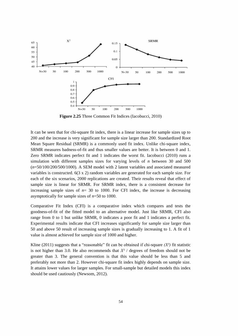
54

Figure 2.25 Three Common Fit Indices (Iacobucci, 2010)

It can be seen that for chi-square fit index, there is a linear increase for sample sizes up to

200 and the increase is very significant for sample size larger than 200. Standardized Root

Mean Square Residual (SRMR) is a commonly used fit index. Unlike chi-square index,

SRMR measures badness-of-fit and thus smaller values are better. It is between 0 and 1.

Zero SRMR indicates perfect fit and 1 indicates the worst fit. Iacobucci (2010) runs a

simulation with different samples sizes for varying levels of n between 30 and 500

(n=50/100/200/500/1000). A SEM model with 2 latent variables and associated measured

variables is constructed. 6(3 x 2) random variables are generated for each sample size. For

each of the six scenarios, 2000 replications are created. Their results reveal that effect of

sample size is linear for SRMR. For SRMR index, there is a consistent decrease for

increasing sample sizes of n= 30 to 1000. For CFI index, the increase is decreasing

asymptotically for sample sizes of n=50 to 1000.

Comparative Fit Index (CFI) is a comparative index which compares and tests the

goodness-of-fit of the fitted model to an alternative model. Just like SRMR, CFI also

range from 0 to 1 but unlike SRMR, 0 indicates a poor fit and 1 indicates a perfect fit.

Experimental results indicate that CFI increases significantly for sample size larger than

50 and above 50 result of increasing sample sizes is gradually increasing to 1. A fit of 1

value is almost achieved for sample size of 1000 and higher.

Kline (2011) suggests that a “reasonable” fit can be obtained if chi-square (X²) fit statistic

is not higher than 3.0. He also recommends that X² / degrees of freedom should not be

greater than 3. The general convention is that this value should be less than 5 and

preferably not more than 2. However chi-square fit index highly depends on sample size.

It attains lower values for larger samples. For small-sample but detailed models this index

should be used cautiously (Newsom, 2012).

55

2.8.7. SAMPLE SIZE AND STATISTICAL POWER IN STRUCTURAL

EQUATION MODELING

“Power of a hypothesis test” is defined as the probability of rejecting hypothesis when it is

really false.

In SE modeling, hypothesis testing is made on the equality of fitted and actual covariance

matrices.

Mac Callum et al. (1996) calculate required sample sizes for achieving target power

values in SE modeling. They simulate SE models with increasing degrees of freedom for

sample sizes between 100 and 500. The findings reveal that for sample size of 500 perfect

fit can be achieved for degrees of freedom of 70 or higher. Degrees-of-freedom of a model

is calculated as the difference between the number of estimated parameters and number of

actual parameters. Higher degrees of freedom indicates bigger model with more measured

variables.

Many researchers study effects of number of variables on required sample size. Westland

(2010) reviews and summarizes many papers and he calculates a lower bound on the

required sample size for a SE model. His bound is given as follows:

n ≥ 50r²- 450r+1100 (2.19)

where n is sample size and r is the ratio of indicators to latent variables.

2.8.8. SAMPLE SIZE CALCULATIONS BASED ON FACTOR ANALYSIS

Structural equation models are based on factor analysis models. A SE model is a

combination of a measurement model and a structural model. Essentially, a measurement

model is based on factor analysis so factor analytic sample size levels should also be

considered for finding the best possible sample size for a SE model.

Two most widely used references in this field are Marsh et al. (1994)’s paper and

MacCallum et al.’s (1996) paper.

Marsh et al. (1994) evaluate effects of different sample size for different p/f (number of

indicators/number of latent variables) ratios. They conduct simulation studies for 3 factor

models with differing no. of indicators per factor. They study effects of p/f for fixed

sample sizes for obtaining proper (convergent) statistical solutions. The results show that

for p/f=4 and 6 percentage of proper statistical solutions significantly improved. The best

results (proper statistical solutions) are obtained for all sample sizes if number of

indicators is 12.

Marsh et al. (1994) also study effects of sample size and p/f for goodness-of-fit statistics.

They show that chi-square and p-values improve significantly as no. of indicators/factor

56

increased. The best solutions (the least number of statistically improper solutions) are

obtained for 4 indicators/factor cases.

Marsh et al. (1994)’s results can be summarized as follows;

-With n=100, p/f should be at least 4.

-With n>100, p/f can be set at 2 or 3.

-Smaller p/f ratios can be suitable for smaller samples but p/f should increase for larger

sample sizes.

-Factor loadings are more equivalently distributed for larger sample sizes (n=400 or

n=1000) and for 3, 6, or 9 indicators per factor.

Mac Callum et al. (1996) study the effects of to number of variables (p) and to expect

(targeted) levels of communalities. They generate data sets based on 20 measured

variables and 3 or 7 factors, with three levels of communalities; high, wide and low. Their

findings suggest that a condition for obtaining sample factors can be to have high

communalities and strongly determined factors (p/f= 10:3 or 20:3). Their findings also

support that best statistical results can be obtained with larger sample sizes.

2.8.9. SAMPLE SIZE CALCULATIONS BASED ON SAMPLING THEORY

Sümbüloğlu and Sümbüloğlu (2009) give exact statistical formulas based on probability of

occurrence of an event and the population size. Formulas for two distinct cases are as

follows:

(N is population size, p is the probability of occurrence of the observed event, d is the

allowed deviation according to p value and t is the t-value for the set degrees of freedom

and for the allowed error level)

1. 2

2)1(

d

pptn

, if population size (N)is unknown, (2.20)

2. )1()1(

)1(22

2

pptNd

ppNtn

, if population size (N) is known. (2.21)

Practical applicability of the above formulas depends on prior knowledge of p and N. A

quick estimate for p can be given as 0.50. In SEM research, p can be taken as the

probability of occurrence of an indicator variable of the target endogenous latent variable,

as a very general approximation.

57

2.8.10. FIT INDICES FOR STRUCTURAL EQUATION MODELS

The goal in SEM is to construct a model that fits the sample data. Therefore, minimum

difference between sample covariance matrix and population covariance matrix, in other

words, a non-significant chi-square is desired. However, chi-square values are highly

inflated when the sample size is large. For this problem, lots of fit indices are developed

that examine model fit while eliminating or minimizing the effect of sample size. One

indicator of a good fitting model is when the ratio of the chi-square value to the degrees

of freedom is less than two (Arıkan, 2010). The independence chi-square test value

should be always significant. Null hypothesis in this test is that there is no

relationship among variables. Therefore, significant independence chi-square test means

that there is some relationship among variables (Arıkan, 2010).

Newsom (2012) favors the use of IFI and TLI indices due to their sample size

independence.

A list of commonly used fit indices is given below:

1. Parsimonious Fit Indices (PGFI, PNFI, PNFI2, PCFI)

These indices reward the less complicated (“less parsimonious”) models. The more

complex is the model the lower is the fit index. The authors strongly recommend the

use of parsimony fit indices in tandem with other measures of goodness-of-fit

however, because no threshold levels for these statistics have been recommended it

has made them more difficult to interpret. The most commonly used one is the

Parsimony Goodness of Fit Index (PGFI). There are no exact threshold values

recommended. Two suggested values are 0.50 and 0.90.

2. Non-centrality-based Indices (RMSEA, CFI, RNI, CI, ECVI)

The most commonly used one is the root mean square error of approximation

(RMSEA) index. This index estimates the lack of fit by comparing perfect

(saturated) model and estimated model using degrees of freedom. RMSEA ranges

from 0 to 1 and values less than 0.06 means a good fitting model. If RMSEA value

is higher than 0.10, this means a poor fitting model (Arıkan, 2010).

Expected Cross Validation Index (ECVI) is used to assess the likelihood that a

proposed model in a single sample will cross-validates with same population of close

sample size. To evaluate ECVI values, ECVI index is calculated for several models

and a model with the smallest ECVI value has the greatest possibility to cross-

validate. Therefore, the smallest value of ECVI is better.

58

2.9. LITERATURE REVIEW ON MODERATED STRUCTURAL EQUATION

MODELING

A typical moderated regression model is given in Figure 2.26. In this model, M is a

categorical variable which moderates the relationship between two continuous variables;

X, the independent variable, and Y, the dependent variable.

Figure 2.26 Moderated Regression This model is also called an “interaction” model in regression.The path model and

statistical explanation of moderation process is given in Figure 2.27.

Figure 2.27 A Moderated Regression Path Model In the above model, the dependent variable Y is regressed upon the independent variable

X. This relation is moderated by a categorical / continuous variable M. The X x M

variable represents the “interaction” effect of M on X-Y relationship. Independent

variables, X and M are mean-centered before calculating the product term to avoid multi-

collinearity. The particular interaction hypothesis for the above model can be stated as;

“M moderates X-Y relationship”. This means that dependence of Y on X is affected by the

level of the moderator variable, M.

An interaction plot gives a general sense of the interaction as in Figure 2.28. This plot

gives the levels of Y attained by changes in X under 2 different levels of A; the moderator

variable.

59

Figure 2.28 An Interaction Plot

The SEM counterpart of this is a model which involves interactions between latent

variables and covariate variables or other latent variables. A typical SEM interaction

model is shown in Figure 2.29 (Kenny and Judd, 1984):

Figure 2.29 A Moderated SE Model (Kenny and Judd, 1984)

In this model, there are two exogenous variables, 1 and 2 affecting the third endogenous

variable, .The model also contains a third exogenous variable, 3, which is the newly

created interaction variable. The indicators of the newly created interaction variable are

obtained as the possible product combinations of the indicators of the constituent latent

variables. Thus the indicators of 3 are x5 (=x1 x x3), x6 (=x1 x x4), x7 (=x2 x x3) and x8

(=x2 x x4). Bollen (1989) gives a heuristic list of rules for constructing the new indicator

variables. These can be summarized as follows:

Each non-scaling indicator of the first latent variable can be multiplied by the non-

scaling indicators of the second interacting latent variable. This is repeated until all

possible pairs of indicators are formed.

All exogenous variables are included in the new model.

60

Here “non-scaling indicators” are those indicator variables whose loadings are not fixed to

one. The following model contains 3 latent variables, each having two indicators. For each

latent variable, one loading is fixed to one. This means y1, y3 and y5 are selected as the

“scaling” indicators. These are the indicators whose one unit changes are reflected as one

unit changes of the linked latent variables. This can result from researcher’s intention, the

wording of the question and / or its response patterns.

Figure 2.30 A SE Model with Scaling Indicators (Hayduk and Littvay, 2012)

Here “non-scaling indicators” are those indicator variables whose loadings are not fixed to

one. This model contains 3 latent variables, each with two indicators. For each latent

variable, one loading is fixed to one. This means y1, y3 and y5 are selected as the “scaling”

indicators. These are the indicators whose one unit changes are perfectly reflected to the

associated latent variables.

SE models with interaction effects are also called “moderated SE models”. Here the term

“moderation” has a similar context as in multiple regression.

Cortina et al. (2001) review available “constrained” techniques for interaction effects in

SEM. These techniques enable formation of product of many indicators as the indicators

of the newly formed interaction latent variable. They provide constraints on the factor

loadings of the indicators of interaction latent variable.Their conclusions are as follows:

Centering the constituent data items is helpful for obtaining better solutions

The product latent variable can be measured with a single indicator term.

Maximum likelihood estimation works well if normality is not severely violated.

Joreskog and Wang’s (1996) and Jaccard and Wan (1995) approaches are the best

working methods for computing interactions. Jaccard and Wan approach forms many

indicators for the product latent variable and the loading of the first one is set to zero.

Joreskog and Wang approach, on the other hand, suggests a single indicator for the

product latent variable.

The above methods mainly assume normality and they do not guarantee an exact solution

for multivariate non-normal data sets. Further they assume that the latent variables are

normally distributed which can is not the case for many real life settings. Marsh and Hau

(2004, 2006) suggest the use of an “unconstrained “approach for testing interaction

61

effects. Here the new product latent variable has the product of centered data as its

indicators with no constraints on factor loadings and path coefficients. Hancock (2012)

provides examples and LISREL codes for this approach. The mean of new interaction

latent variable is set to be equal to the covariance between the constituent latent variable.

The means of the constituent latent variables are set to zero. Steinmetz et al. (2011)

provide a comparison of unconstrained, residual-centering and constrained approaches for

interacting effects of an individual’s intention to perform a behavior and perceived

behavioral control on behavior for 1442 respondents. They conclude that the first two

approaches are more easily implemented using the most commonly used SEM software

like LISREL, Mplus, AMOS, EQS or Mx.

62

63

CHAPTER 3

MODELING AND ANALYSIS STRATEGIES

3.1. THE MODEL SPECIFICATION

We have conducted an extensive literature research on customer satisfaction and loyalty in

various service and goods settings. The detailed results are given in Chapter 2. We have

finalized our model based on ten latent variables and five covariates. Based on the

customer satisfaction index studies and customer satisfaction – loyalty research on various

service settings we have specified our conceptual model as a SE model with 10 latent

variables, five covariate variables and 37 questions. The latent variables are listed below:

Company Image/ Reputation

Communications

Perceived Quality

Perceived Value

Customer Satisfaction

Customer Expectations

Commitment

Trust

Loyalty

Insensitivity (Sensitivity) to Competitive Offerings

37 initial items are formulated to measure the latent variables. Those are derived from the

validated items in the relevant literature. Ratio of items to latent variables is 3.7, and this

is greater than three in line with the recommendations in SEM literature.

Five covariate variables are formulated based on industry experts’ opinions. Unlike latent

variable questions, each covariate is assumed to be measured without error and with a

single question. These can also be called as “control variables” in our research model.

These variables are measured by five items. The covariates are as follows:

Length of Relationship

Prior Research on Legislations

Average Monthly Household Income

Knowledge of Laws and Legislations During Pre-Purchase or Renewal

Household Education Level

64

3.2. SPECIFICATION OF OUR MEASUREMENT MODEL

We have hypothesized a ten-factor model with 37 indicator variables. Each indicator

question corresponds to a questionnaire item. The detailed breakdown of questions is

given in Chapter 4.

3.3. SPECIFICATION OF A STRUCTURAL MODEL

We have hypothesized a ten-factor model where the ten factors are measured by 37

indicator variables. Each indicator question corresponds to a questionnaire item. The

codes are used throughout the analysis and the results are also discussed with these new

item codes. The administered survey is given in Appendix A.

The following hypotheses are formulated for the 10 latent variables. The literature

references are provided in parentheses (The relevant details are provided in Chapter 2):

1. Satisfaction has a positive impact on Loyalty (Anderson and Fornell, 2000, and

industry experts, 2010).

2. Satisfaction has a positive impact on Commitment (Fullerton, 2011, and industry

experts, 2012)

3. Commitment has a positive impact on Loyalty (Cater and Cater, 2010).

4. Insensitivity to Competitive Offerings has a positive impact on Commitment

(industry experts ‘opinions).

5. Trust has an impact on Insensitivity on Competitive Offerings (Akgözlü, personal

communications in 2012).

6. Perceived Value has a positive impact on Satisfaction (Anderson and Fornell, 2000).

7. Perceived Quality has a positive impact on Perceived Value (Anderson and Fornell,

2000).

8. Perceived Quality has a positive impact on Satisfaction (Anderson and Fornell,

2000).

9. Company Image has a positive impact on Trust (Türkyılmaz and Özkan, 2007).

10. Company Image has a positive impact on Expectations (Türkyılmaz and Özkan,

2007).

11. Expectations has an impact on Perceived Value (Türkyılmaz and Özkan, 2007,

personal communications with T. Akgözlü in 2012).

12. Expectations has a positive impact on Perceived Quality (Türkyılmaz and Özkan,

2007).

13. Expectations has a negative impact on Satisfaction (Türkyılmaz and Özkan, 2007).

14. Communications has a positive impact on Loyalty (Ball et al., 2004).

15. Communications has a positive impact on Satisfaction (Ball et al., 2004).

16. Communications has a positive impact on Trust (Ball et al., 2004).

17. Insensitivity to Competitive Offerings has a positive impact on Commitment

(personal communications with T. Akgözlü in 2012).

3.3.1. SPECIFICATION OF THE EXTENDED STRUCTURAL MODEL WITH

COVARIATES

The hypotheses for covariate- latent variable relations are listed below (Relevance

assessment studies are conducted with academics and industry experts during content

validity research. The process is given in Section 3.4):

65

Length of Relationship has an impact on Customer Satisfaction.

Length of Relationship has an impact on Perceived Quality.

Length of Relationship has an impact on Perceived Value.

Length of Relationship has an impact on Trust variables.

Length of Relationship has an impact on Loyalty.

Length of Relationship has an impact on Communications.

Income of the user has an impact on Customer Satisfaction.

Household’s Income Level has an impact on Commitment.

Income of the user has an impact on Perceived Quality and Value.

Household’s Education Level has an impact on Commitment.

Household’s Education Level has an impact on Loyalty.

Household’s Education Level has an impact on Perceived Quality.

Household’s Education Level has an impact on Perceived Value.

Household’s Education Level has an impact on Customer Expectations.

3.3.2. HYPOTHESIZED RELATIONS BETWEEN COVARIATES AND LATENT

VARIABLES IN THE BASE MODEL

The hypotheses for covariate- latent variable relations are listed below (Relevance

assessment studies are conducted with academics and industry experts):

Price considerations have an impact on Perceived Value.

Price considerations have an impact on Sensitivity to Competitive Offerings construct.

Length of Relationship has an impact on Satisfaction.

Length of Relationship has an impact on Perceived Value.

Length of Relationship has an impact on Trust.

Length of Relationship has an impact on Loyalty.

Length of Relationship has an impact on Communications.

Income of the user has an impact on Loyalty.

Income of the user has an impact on Perceived Value.

Income of the user has an impact on Perceived Quality.

Income of the user has an impact on Customer Satisfaction.

Income of the user has an impact on Commitment.

Household’s Education Level has an impact on Commitment.

Household’s Education Level has an impact on Perceived Quality and Value.

Household’s Education Level has an impact on Customer Expectations.

3.4. CONTENT VALIDITY OF HYPOTHESIZED RELATIONS

The preliminary hypotheses are discussed with a group of six academicians (Kavak, B.,

Köksal,G., Yozgatlıgil, C., Ekici, A., Gürel, E., Coşkun,N., 2009-2013) and three industry

experts (Akgözlü, T., Oktay, Ş., Pakkan, A.) from leading AC manufacturers. We have

used a two-step expert judgment process as follows:

1. The experts are asked about their general understanding of the model and the

variables. They make suggestions for revisions and necessity of some latent

variables and covariates. These shed light on the variable definitions. Academic

experts suggested removing some variables but industry experts stated necessities

66

for real-life scenarios. These “suspected” variables are checked for their factor

analysis results. Low-loading and unloaded variables are completely removed

from the model.

2. The experts are asked to check the relevance of causality relations between latent

variables and covariates. Answers are marked as YES for a cell (i, j) if the causal

path latent variable I to causal path latent variable j is suspected or observed by

the experts. The most agreed paths are maintained in the final model. The 1-YES

paths are deleted. This assessment provides a preliminary screening of the paths in

the structural model. Number of paths is reduced. The model thus becomes more

parsimonious. “Parsimony” in SEM can be defined as; “expressing the underlying

theory with the simplest sets of assumptions and with the least number of

variables”. Among 54 paths asked, 25 are agreed by at least two of the experts.

Thus the final model has 25 causal paths between latent variables and paths from

covariates to latent variables. The content validity tables have the following

matrix structures:

Table 3.1 Experts’ Content Validity Checks-First Table

Path From\ To LATENT VARIABLE 1 LATENT VARIABLE 2 LATENT VARIABLE 1 LATENT VARIABLE 2

Table 3.2 Experts’ Content Validity Checks-Second Table

Path From To LATENT VARIABLE 1 LATENT VARIABLE 2 COVARIATE 1 COVARIATE 2

Experts are also asked to check the relevance of covariates and latent variables. The

results are summarized as follows:

Length of relationship is a significant covariate. This is asked on a continuous scale.

Company’s operational capability can be assessed within different latent variables, it is

not clear–THIS COVARIATE IS REMOVED.

Company’s communications capability assessment can be assessed within different

latent variables, it is not clear–THIS COVARIATE IS REMOVED.

Company’s core capability assessment question is not clear to the respondent – THIS

COVARIATE IS REMOVED.

“Price considerations” is a significant covariate.

Income of the user is a significant covariate. This is asked as an interval.

“Alternative offers” is a significant covariate. But it can lead to redundant paths since

there is also a latent variable with the same name. –THIS COVARIATE IS

REMOVED.

Awareness of legislative / initial agreements is a significant covariate.

Household’s education level is added as a covariate.

Among 70 paths asked (7 covariates x 10 latent variables), 63 are agreed by all the

experts. The paths of removed covariates are also removed from the path model.

67

3.5. DETAILED EXPLANATION OF OUR RESEARCH MODEL

Suggested path model of the research problem is given in Figure 3.1. The model contains

10 latent variables, their indicator variables and five covariates. Each latent variable is

measured through its indicator variables. The model consists of three major components;

the structural model, the measurement model with latent variables and their indicators and

the measurement model with covariates and related paths. These are detailed in the

following sections.

3.5.1. THE STRUCTURAL MODEL

The structural model comprises all the equations relating latent variables in our model.

These are based on the hypothesized relations between latent variables (see Figure 3.1).

For two of the latent variables, the path model is detailed in Figure 3. 2. The associated

matrix equations can be written as follows:

η = Βη + Γξ + ζ (3.1)

Figure 3.1 Suggested Path Model for the Research Problem

In equation (3.1), η is the m×1 vector of latent endogenous variables, ξ is the (m+p) ×1

vector of latent exogenous variables, B is the m x m matrix of path coefficients of causal

links connecting endogenous variables to all other endogenous variables, Γ is the (m+p) ×

(n+q) matrix of path coefficients of paths (causal links) connecting endogenous variables

to exogenous observed variables and ζ is the m × 1 vector of disturbance random variables

on the endogenous latent variables. A complete list of conventional SEM notations

(Newsom, 2012) is given in Appendices.

68

3.5.2. STRUCTURAL MODEL EQUATIONS

The full model can be broken into smaller models as follows:

Figure 3.2 A Sub-model of the Research Problem

For the above sub-model, there are two latent variables:

PERCEIVED VALUE is the endogenous latent variable

PERCEIVED QUALITY is the exogenous latent variable

There is a disturbance term associated with PERCEIVED VALUE, which accounts for the

unexplained part of the model or the expected lack of explanation of the endogenous

variable by its indicators and by its predecessor which is the exogenous variable. The

structural equation can be written as follows:

PERCEIVED VALUE = βPQ,PV PERCEIVED QUALITY +ζ (3.2)

Here, βPQ,PV is the path coefficient and ζ is the disturbance term of PERCEIVED VALUE.

This equation then can be repeated for all paths connecting an exogenous latent variable to

an endogenous variable. This equation is obtained from equation (3.1). An endogenous

latent variable, PERCEIVED VALUE is connected to a latent exogenous variable,

PERCEIVED QUALITY and the disturbance term.

3.5.3. THE MEASUREMENT MODEL

This is the collection of all measurement equations of the model. These are the equations

relating latent variables and measured variables (indicator variables). These form the

“factor analysis” part of the full model. The equations are as follows:

y = Λ y η + ε

x = Λ xξ + δ (3.3) In the above sets of equations, Λx (q x n) and Λy (p x m) represent the factor loading

matrices. Each entry of these matrices correspond to a factor loading coefficient relating

one latent variable to one measured variable (or the “indicator”). ε and δ are the

measurement errors associated with the measured variables x and y, respectively. The first

equation relates measured dependent variables to endogenous latent variables and error

terms. So it can be named as the “dependent variables’ equation”. The second equation

relates measured independent variables to exogenous latent variables and error terms.

69

3.5.4. MEASUREMENT MODEL EQUATIONS

Taking a small part of the research model without a covariate, we can exemplify

the measurement equations as follows:

Figure 3. 3 A Sub-model of our Research Problem

In the above sub-model, the exogenous latent variable is Perceived Quality (PQ). Perceived

Value (PV) is the endogenous latent variable. Let us assume that the number of indicators of

PQ is 3 (question 1 score (qPQ,1), question 2 score (qPQ,2) and question 3 score (qPQ,3)) and

that of PV is again three (question 1 score (qPV,1), question 2 score (qPV,2) and question 3

score (qPV,3)). The relevant measurement equations can be written as follows:

qPV = Λy . PV + ε1

qPQ = Λx . PQ + ε2 (3.4)

We can re-write the above equations, this time for a covariate sub-model. Let us assume

that the sub-model is as follows:

Figure 3.4 A Confirmatory Factor Analysis Sub-model

In the above sub- model, we have three covariates affecting SATISFACTION, the latent

variable. This latent variable is connected to three indicator variables. The associated

measurement equations are as follows:

SATISFA = βi COVi +ζ for i=1,2,3

yi = i SATISFA+εi for i=1,2,3 (3.5)

70

3.5.5. MATRIX EQUATIONS FOR THE FULL MODEL

A full SE model is given in Figure 3.5.

Figure 3.5 A Full SE Model (Rigdon, 1996)

Figure 3.6 An Extended SEM with Covariates (MIMIC Model)

The matrix equations for the full model are given as follows:

(3.6)

In the above sets of equations, is the m×1 vector of latent endogenous variables, y is the

p×1 vector of measurable endogenous variables, A is the (m+p) × (m+p) matrix of path

coefficients of causal links connecting endogenous variables to all other endogenous

variables, Γξ is the (m +p) × n matrix of path coefficients of paths connecting endogenous

variables to exogenous observed variables, Γx1 is the (m +p) × q1 matrix of path

coefficients of paths connecting endogenous variables to exogenous observed variables, x1

(q1 ×1), Γx2 is the (m +p) × q2 matrix of path coefficients of paths connecting endogenous

71

variables to exogenous observed variables, x2 (q2 ×1), (q1 + q2) being equal to q; the total

number of measured variables. The principle diagonal of A contains zeros because no

endogenous variable can be a cause of itself. is the m × 1 vector of disturbance random

variables on the latent endogenous variables. , is, again, the matrix of path coefficients

relating all variables to their measurement errors (for indicators) or disturbances (for latent

variables). Ψ is a p × p diagonal matrix of structural coefficients relating measurable

endogenous variables to exogenous disturbance variables and x is the vector of exogenous

indicators. An extended SE model with both causal and also resulting variables is given in

Figure 3.6.

This is called a MIMIC (Multiple Indicators Multiple Causes) model. Examples of

MIMIC models are given in Chapter 2.

3.6. HYPOTHESIZED MODERATED RELATIONS AS A FURTHER

EXTENSION OF THE MODEL

The following statements hypothesize the interaction effects of covariates and other latent

variables in our research problem. The hypotheses are based on industry experts’ opinions

on customer attitudes.

We have conducted preliminary analyses with our data and we observed some interaction

effects. These new hypotheses are also added to our model. These interaction effects are

expected to strengthen the effects of covariates on the latent variables.

Length of Relationship moderates the relation between customer satisfaction and

loyalty (Pakkan, Akgözlü, Oktay, 2012).

Length of Relationship moderates the relation between Perceived quality and

perceived value (Pakkan, Akgözlü, Oktay, 2012).

Length of Relationship moderates the relation communication and customer

satisfaction (Pakkan, Akgözlü, Oktay, 2012).

Household’s Income Level moderates the relation between customer satisfaction and

loyalty.

Household’s Income Level moderates the relation between Perceived quality

and perceived value. Household’s Education Level moderates the relation between commitment and loyalty.

Household’s Education Level moderates the relation between Perceived quality and

perceived value.

The above relations are first tested using interaction plots. These are visual displays of

possible interaction effects but they do not necessarily indicate statistically significant

moderations. The graphs are plotted using the mean of the indicator measurements (“latent

means”) for each latent variable. The interaction plots are given in Chapter 5.

The relations are then tested using a SPSS macro named “PROCESS” (Hayes, 2012),

which is a composite moderation-mediation testing software. Unlike stepwise regression,

this tool computes combined moderation and mediation effects in a composite manner.

72

Finally the interaction relations are tested using unrestricted interactions approach of

Marsh et al. (2004). For these structural equation models, covariate variables are re-

formulated as single-indicator latent variables as shown in Figure 3.7. These are also

called “phantom” variables. These are variables with no substantive meaning and they do

not have disturbances. They do not contribute to the model fit, the implied covariance

matrix, and the parameter estimates some SEM software forces the user to use these

variables because of the reduced complexity of connecting latent variables to other latent

variables rather than connecting measured variables as direct causal variables to latent

variables.

Figure 3.7 Covariates Modeled with a Pseudo-Latent (Phantom) Variable

3.7. ANALYSIS STAGES

We follow Bollen’s (1989) six-step analysis and testing procedure in our detailed SEM

analyses. In the re-specification stage, we can;

1. Combine or drop some factors depending on the values of factor loadings in an

alternative modeling effort.

2. Revise the model (add a new factor onto which indicators with correlated error terms

are loaded) according to modification indices.

3. Drop some factors based on violations of uni-dimensionality or modification indices.

3.8. LONGITUDINAL MODELING POSSIBILITIES AND REASONS OF NOT

ADAPTING THIS APPROACH

The following conditions should be checked for developing a longitudinal study

framework:

There should be continuous outcomes that change systematically over time.

There should be multiple waves of data for the same persons and number of waves

should be greater than 2 to model individual changes over time.

73

Little et al.(2009) list advantages of longitudinal modeling for studying developmental

changes in psychology. Their arguments can equally be applied to our research field as

follows:

Longitudinal analysis allows researchers to study cross-time differences in

respondents’ attitudes.

Through longitudinal modeling, we can model the processes through which effects are

expressed over time. Through data collected at multiple time points, both direct and

indirect pathways of influence can be modeled.

Farrell (1994) studies the effects of level of anger on peer alcohol use and alcohol use.

This model aims to examine anger-peer alcohol use-alcohol use effects over three time

periods. The properties of the model are as follows:

Error terms of indicators at different time periods are correlated by modeler’s

decisions.

These two-sided arrows account for autocorrelations in time series analysis.

Each latent variable is connected to its counterpart in the immediately succeeding wave

and also to all latent variables in the succeeding wave as set in the theoretical model.

Preliminary interviews with experts reveal the presence of three distinct phases in the

consumption process of heating and air conditioning products. These are:

1. Pre-purchase phase: When the customer evaluates alternatives and his/her prior

experience before engaging in purchase.

2. Purchase phase: When the customer buys and utilizes the product. This phase does not

involve long-term consequences of consumption experience. It covers the warranty

period.

3. Post-purchase phase: It includes factors related with “cumulative” consumption

experience.

Based on industry experts’ opinions and our findings from the existing surveys of durable

goods manufacturers, we detail measurement characteristics of latent variables below.

Consumption process of durable goods points to the existence of three phases. However

these do not necessarily correspond to measurement occasions.

Heating and ventilating products are used for at least 10 years. This period can extend

up to 15 years for Turkish consumers.

Customer opinions start to form after one season’s (one year’s) utilization. A “season”

is meant to cover utilizing a product for one summer term or over one summer and one

winter term. The customer starts to form satisfaction and loyalty ideas. In and after the

third year of utilization (warranty period of these types of products is three years)

loyalty is formed.

“Customer expectations” is a latent variable which covers the initial starting

experience. It does not affect the customer throughout usage period in the post-

purchase period.

“Perceived quality” is a latent variable which need not be assessed in all periods of

product use. It can be measured in “pre-purchase” phase and for only once.

74

“Perceived value” is a factor which can be assessed during purchase and post-purchase

periods.

Trust is a factor which forms prior to purchase of a product and is an important trigger

in purchasing decisions. It can be measured in the intermediate waves and not in the

starting measurement occasion. It need not be assessed in the post-purchase

measurement periods, since it is formed and does not change over time. Instead it is

reflected as a part of customer satisfaction and indirectly as a part of customer loyalty.

“Company image” is a factor which is formed prior to purchasing decision. It is

strengthened during consumption process. It is to be assessed in the later measurement

occasions.

Communication is a factor which affects the purchasing decision. It also affects

customer’s impressions in the post-purchase period.

Customer satisfaction is the consequence of a cumulative experience. It is measured

only in the post-purchase phase.

Customer loyalty is the consequence of a cumulative experience. It is measured only in

the post-purchase phases.

Insensitivity to Competitive Offerings is a mediating factor on loyalty. It plays role in

the renewal and pre-purchase phases. It is not important in intermediate phases of

consumption.

Our findings point to the following facts:

1. Satisfaction forms after a one-season or one year of usage of the purchased good. At

the end of one season’s (or one year’s usage) loyalty starts to form.

2. The common minimum utilization period after the purchase of a good is 1 year.

3. Customer complaints may occur within one year’s time or after that. The resolution of

complaints in the warranty period strengthens loyalty and reduces customers’ search

for competing suppliers. Complaints will not be handled as a separate latent variable in

our research.

4. Loyalty forms after a cumulative consumption experience. If a customer is loyal, then

s/he starts to make good recommendations. Thus loyalty is a post-purchase latent

variable.

5. The common warranty period for the heating/cooling devices is three years. Thus the

customers need to be observed for one to three or more than three years of usage for

the most realistic results.

6. Perceived quality and expectations form prior to purchase and are strengthened or

weakened during consumption or utilization period.

We can say that there are distinct consumption phases in our problem. There are

differences in customer attitudes over these distinct consumption phases. Some latent

variables can be observed over some consumption phases and not over the others. This

points to the fact that “length of use of a product” should be a major causal variable in the

model. “Length of use” can be incorporated into the baseline model in two ways:

Some or all of the latent variables can be replicated over periods, which can be taken as

“seasons” or “years”. Thus the baseline model can be extended to cover more than one

point in time. This is longitudinal modeling approach.

Length of use can be added as a covariate to the baseline model and its relations with latent

variables can be analyzed for significance. This can also lead to a “grouping” strategy.

75

We have adapted the second strategy due to the following drawbacks of longitudinal

modeling:

Responses for perception variables are prone to recall biases.

Repeated data collection at different time points is not feasible due to respondents’

attrition and our time limitations.

In the consumption setting, ten latent variables do not all have the same repeating

patterns. Thus it is impossible to construct a model similar to Farrell’s (1994)

longitudinal model.

Some latent variables can repeat over all consumption phases and some others can

become constant over time.

3.9. MULTIGROUP MODELING POSSIBILITIES

“Length of use” can also be added as a grouping variable to our model as follows:

Customers in the first group are the “new” users of a good. They have been using the

product for at most one year. Some of the latent variables are expected to drop from the

path model. Some of the latent variables are expected to be dropped due to stated

observations in Section 3.8.

Customers in the second group are the “relatively mature” users of a good. They have

been using the product for one to three years, three years being the generally accepted

warranty period for durable goods. Some of the latent variables are expected to drop

from the path model. The baseline model given in Figure 3.1 can be tested as a whole.

Some of the latent variables are expected to be dropped due to the observations stated

in Section 3.8.

Customers in the third group are the “mature” users of a good. They have been using the

product for at least three years. The baseline model can be tested as a whole. The full

model is expected to appear significant after the analysis. Satisfaction, loyalty and

insensitivity (to competitive offerings) are expected to form only for this group of users.

3.9.1. MULTIGROUP MODELS AS EXTENSIONS OF MIMIC MODELS

Two types of SE models are presented to analyze the difference in means: multiple-group

models and multiple-indicator, multiple-cause models. The multiple-group models may be

conceptualized as analogous to ANOVA models, whereas MIMIC models may be thought

to be analogous to regression models.

We can test group differences for users with different lengths of use based on MIMIC

models with the following different hypotheses for different models:

1. Factor patterns are the same.

2. Error variances are the same.

3. Factor covariances are the same.

76

3.10. DIRECT EFFECT OF LENGTH OF RELATIONSHIP

We can link the length of relationship covariate to all the latent variables to assess the

effects of different utilization periods over consumer perceptions. This will increase the

number of paths and will complicate the solution. Instead practical solution strategies can

be suggested as follows:

1. Length of relationship covariate can be linked to “loyalty” latent variable only.

The model can be analyzed accordingly. Depending on the results, the covariate can be

gradually linked to other latent variables to assess its effects on other latent variables.

2. Step 1 can be repeated for satisfaction which is one of predecessors of loyalty variable.

Model in this step can be gradually expanded to incorporate other latent variables

(except for pre-purchase latent variables like trust and perceived quality) until a

convergence problem occurs. Convergence problems can occur due to increasing

number of parameters to be estimated compared to the number of available data points.

Identification problems can also occur. Details of “identification” problem are

discussed in Chapter 2. These problems can be overcome by proper elimination of

unnecessary paths or insignificant variables. These are discussed in Chapter 4.

3.11. EXPLORATORY FACTOR ANALYSIS WITH PILOT QUESTIONNAIRE

DATA

SEM involves testing a priori hypotheses. It is a confirmatory statistical tool. However,

with the use of exploratory factor analysis, the number of factors can be tested with a pilot

data set before starting with the final SEM analysis. The loadings and number of extracted

components can be tested before starting with the final SEM analysis. This can lead to the

following:

Number of factors can decrease. The hypothesized latent variables should be revised

before SEM analysis.

Some items can be loaded onto different factors. The questions can be revised before

the final questionnaire is applied.

Some of the items may remain “unloaded”. These questions can be eliminated

orrevised for the final questionnaire.

3.12. PRIOR MEDIATION AND MODERATION ANALYSES

We have mediation and moderation hypotheses in our formulations. Most SEM software

cannot check the presence of mediation and moderation with small samples or in the

presence of high inter-item correlations. Thus we have conducted preliminary screening to

simplify SEM software coding process.

We use SPSS PROCESS tool (Hayes, 2012) for recursive loop structures. This is an SPSS

MACRO. It uses an ordinary least squares or logistic regression-based path analytical

framework for estimating direct and indirect effects in simple and multiple mediator and

moderator models. It has 74 moderation / mediation test options for different recursive loop

structures. We use Model 1 and Model 4 with the structures shown in Figures 3.8 and 3.9.

These are the basic mediation and moderation templates in PROCESS software. The

structures are shown in Figures 3.8 and 3.9. The conceptual and path models are provided

simultaneously.

77

Figure 3.8 SPSS PROCESS Tool’s Model for testing mediation effects (Hayes, 2012)

Figure 3.9 SPSS- PROCESS Tool’s Model for testing moderation effects (Hayes, 2012)

78

79

CHAPTER 4

DATA COLLECTION AND ANALYSIS

4.1. SAMPLING DESIGN

A good sample design should ensure that the specification of the target population is

clearly and completely defined. Our target population is defined as the “frequent AC

users” in Turkey. The manufacturer companies define “frequent” users as “the households

who are using an AC device for at least two months in a year”.

Geographical regions for sampling are chosen on the basis of average air-conditioner

utilization rates compiled from Turkish Statistical Institute’s Household Budget Data.

Data is summarized as to AC ownership ratio in 26 determined geographical regions.

According to the results, the highest AC ownership rates are observed in İzmir, Antalya

and surroundings and Manisa and surroundings. The lowest ownership rates are observed

in Central Anatolia with Ankara as the representative province). The findings are

displayed in the following table:

Table 4.1 AC Ownership Ratios in Some Geographic Regions in Turkey

SELECTED REGIONS AC OWNERSHIP RATIO (%)

İzmir 47.79

Antalya, Isparta, Burdur 37.82

Manisa, Afyon, Kütahya, Uşak 13.89

Ankara 2.35

The average residential AC ownership in Turkey is estimated to be between 10-15%. Unit

of our study is defined as a “household”. There are 19, 842,850 households in Turkey

(TURKSTAT, 2012). We can say that the estimated number of AC-using households in

Turkey is between 1,984,285- 2,976,427. The total number of households in the sampling

provinces is calculated as 4,121,287 and this constitutes 21% of Turkey’s population.

To calculate the sample size we use stratified sampling logic. We assume that a proportion

of the customers (p) s loyal and the remaining proportion (1-p) is not loyal, since loyalty is

our main target variable. The real proportion of loyalty can not be estimated since there is

not a relevant research in Turkey. However, p is approximated as 0.5. The following

formula is used to calculate the sample size (Sümbüloğlu and Sümbüloğlu, 2009):

80

05.0,),1(2

PpTpps p

(4.1)

where;

(4.2)

p is the sample proportion and P is the population proportion for loyalty. The required

sample size, n, is thus calculated as 600. This number is compared to the minimum

required sample sizes for a SEM study (literature findings are presented in Chapter 2). We

conclude that 600 is an adequate sample size for conducting a SEM study. We later

confirm this by considering the number of questions and the required level of fit for our

model.

4.2. DATA COLLECTION

For an estimated average response rate of 0.10, the planned number of survey applications

is thus set as 6000. This number is equally split between web- based and paper- based

applications. Data is collected in two forms:

1. Paper-based survey is administered to groups of residential AC users in different

geographical regions. In line with the above results, 3000 survey forms are mailed to

users residing in İzmir, Antalya, Manisa and Ankara. Number of returned forms is

300. The response rate is 0.10. Data is then entered into METU SURVEY web

medium. METU SURVEY is a survey system with an advanced software

infrastructure provided by provided by METU Computer Center. The survey enables

one-at-a-time or resumed data entry modes. Menu screenshot and data entry screen

pictures are given in Appendix A.

2. Web-based survey is administered to groups of residential AC users in different

geographical regions. 3000 emails containing an introductory text and the

METUSURVEY link are sent to consumers in different regions. The number of filled

entries is approximately 140. The response rate is 0.047.

The total number of sent surveys is thus 6000. The total number of returned surveys is

440. Thus the overall response rate is 0.073. This is lower than our targeted response rate.

Stil this is an adequate sample size for conducting a SEM study (Iacobucci, 2010).

4.3. QUESTIONNAIRE DESIGN

In SEM research, a questionnaire is used as a measurement instrument. The major aim is

to calculate scores for “indicators” via questions. Each question aims to measure one

2

22/

2

T

szn

p

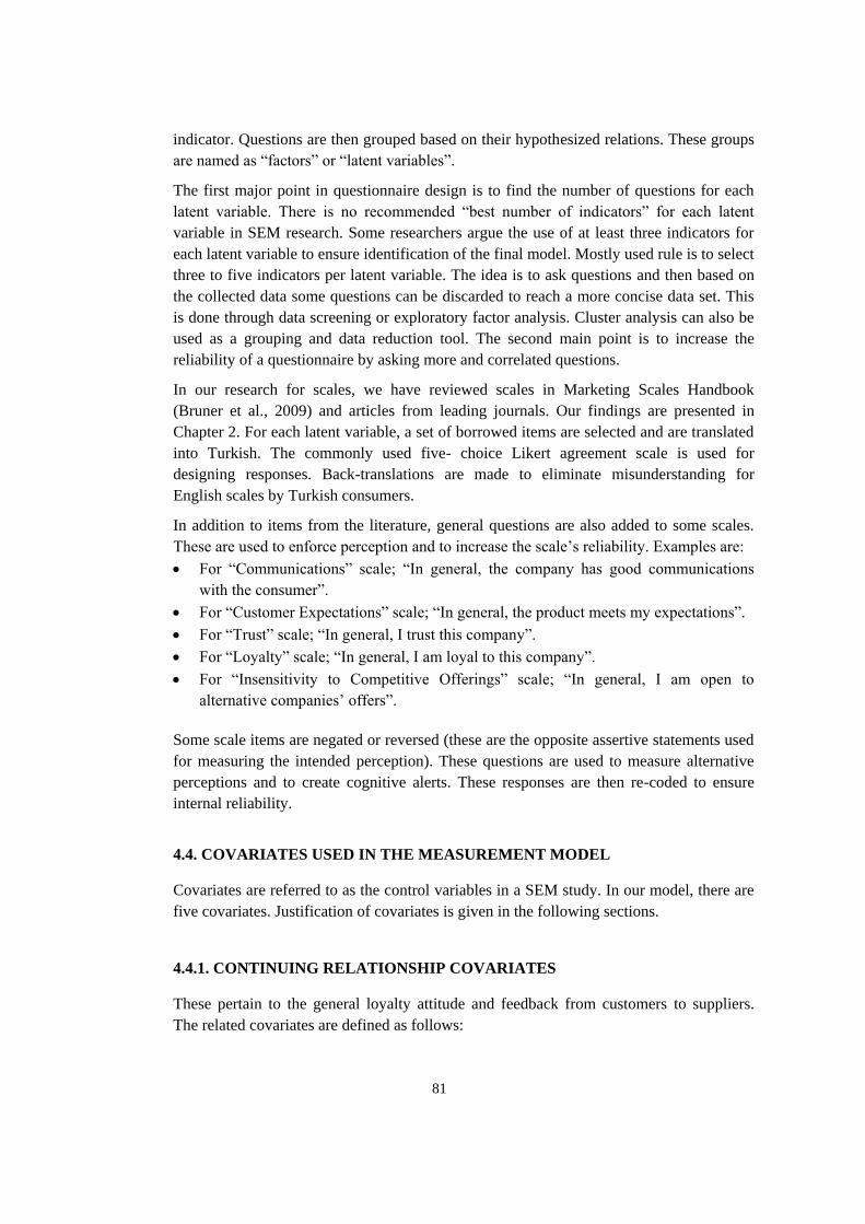
81

indicator. Questions are then grouped based on their hypothesized relations. These groups

are named as “factors” or “latent variables”.

The first major point in questionnaire design is to find the number of questions for each

latent variable. There is no recommended “best number of indicators” for each latent

variable in SEM research. Some researchers argue the use of at least three indicators for

each latent variable to ensure identification of the final model. Mostly used rule is to select

three to five indicators per latent variable. The idea is to ask questions and then based on

the collected data some questions can be discarded to reach a more concise data set. This

is done through data screening or exploratory factor analysis. Cluster analysis can also be

used as a grouping and data reduction tool. The second main point is to increase the

reliability of a questionnaire by asking more and correlated questions.

In our research for scales, we have reviewed scales in Marketing Scales Handbook

(Bruner et al., 2009) and articles from leading journals. Our findings are presented in

Chapter 2. For each latent variable, a set of borrowed items are selected and are translated

into Turkish. The commonly used five- choice Likert agreement scale is used for

designing responses. Back-translations are made to eliminate misunderstanding for

English scales by Turkish consumers.

In addition to items from the literature, general questions are also added to some scales.

These are used to enforce perception and to increase the scale’s reliability. Examples are:

For “Communications” scale; “In general, the company has good communications

with the consumer”.

For “Customer Expectations” scale; “In general, the product meets my expectations”.

For “Trust” scale; “In general, I trust this company”.

For “Loyalty” scale; “In general, I am loyal to this company”.

For “Insensitivity to Competitive Offerings” scale; “In general, I am open to

alternative companies’ offers”.

Some scale items are negated or reversed (these are the opposite assertive statements used

for measuring the intended perception). These questions are used to measure alternative

perceptions and to create cognitive alerts. These responses are then re-coded to ensure

internal reliability.

4.4. COVARIATES USED IN THE MEASUREMENT MODEL

Covariates are referred to as the control variables in a SEM study. In our model, there are

five covariates. Justification of covariates is given in the following sections.

4.4.1. CONTINUING RELATIONSHIP COVARIATES

These pertain to the general loyalty attitude and feedback from customers to suppliers.

The related covariates are defined as follows:

82

Relationship duration / being tenure in relation / the number of months of relationship

with the supplier (is assessed through exact number of years and months)

Price considerations - is used in our questionnaire (is assessed through three response

choices)

4.4.2. PRODUCT UPGRADE/CONTRACT RENEWAL DECISION COVARIATES

These covariates pertain to changing/renewing an existing product. In our research

problem, the related covariates are defined as follows:

Relationship duration (is assessed through exact number of years and months)

Customer’s consciousness of market prices for similar products (is assessed through

three response choices)

Customer’s consciousness of legislative/ regulatory constraints (is assessed through

three response choices)

4.4.3. COVARIATES MEASURING DEMOGRAPHIC CHARACTERISTICS

These covariates aim to measure general consumer characteristics. The questions are

chosen on the basis of contacts with industry experts. The response choices (6 choices for

each) are taken from research reports of Turkish Institute of Statistics (TURKSTAT, 2010,

2011). The related covariates are defined as follows:

Household’ average income level (is assessed through six response choices)

Household’s highest education level (is assessed through six response choices)

4.5. BACKGROUND AND ORGANIZATION OF THE QUESTIONNAIRE

The questionnaire is organized in two parts:

PART 1: Contains five questions targeting to measure five covariates. Firstly, a literature

review on purchasing tendencies and loyalty attitudes for consumption of expensive and

durable goods is conducted. Secondly, the covariates are confirmed with academics from

Middle East Technical University, Bilkent University, Hacettepe University and industry

experts from three leading durable goods’ manufacturers. The questionnaire is pilot-tested

with a small group of respondents (with 20 participants, including academics, residential

users and undergraduate students in Bilkent University and Aegean University).

The questions are:

1. How long have you been using your most preferred/ most used AC device?

This is a continous reponse question. The duration of use is given in months. This is

later grouped into four categories:

Group 1: Less than one year

83

Group 2: Betwen 1- 2 years

Group 3: Between 2-3 years

Group 4: More than 3 years

These groups are settled with industry experts based on customer opinions and previous

consumer surveys.

2. Which one shows your household’s average monthly income level?

This is a six-choice question. The categories are as follows:

Group 1: Primary School or lower

Group 2: Primary and Secondary Schools

Group 3: General Lycee

Group 4: Vocational/ Technical Lycee

Group 5: University Degree

Group 6: Graduate Degree

These groups are taken from TURKSTAT’s research reports. The responses are re-coded

into three categories for further analyses (two groups being in each category).

1. Which one shows your household’s highest education level?

This is a six-choice question. The categories are as follows:

Group 1: 700 TL or lower

Group 2: 700- 1000 TL

Group 3: 1000 - 2000 TL

Group 4: 2000-4500 TL

Group 5: 4500 – 10000TL

Group 6: 10000 TL or higher

These groups are taken from TURKSTAT’s research reports. The responses are further re-

coded to less number of categories for more accurate analyses.

PART 2: Contains 37 questions measuring 10 latent variables. These are:

Company Image/ Reputation

Communications

Perceived Quality

Perceived Value

Customer Satisfaction

Customer Expectations

Commitment

Trust

Loyalty

Insensitivity (Sensitivity) to Competitive Offerings

The questions are borrowed from relevant scales in literature. Most of the questions

pertain to service sector applications. Our research aims to measure the applicability of

these to the case of a specific durable good’s consumption. The detailed allocation of

84

questions is given in Table 4.2. The codes used in analyses are given in Table 4.3.The “R”

codes indicate reversed or negated questions.

Table 4.2 Organization of the Questionnaire

PART 1 - COVARIATES

COVARIATE

IS ASSESSED

BY

QUESTIONS

REFERENCES QUESTION

Length of Relationship

with the Company 1

Academicians (personal communications

with Koksal, Yozgatlıgil, Ekici, Kavak in

2012),

Industry experts

How long have you been using

your most preferred/ most used

AC device ?

Price Research Before

Purchasing A Product 2

Academicians(personal communications

with Köksal, Yozgatlıgil, Ekici, Kavak in

2012),

Industry experts

Do you make a price research

prior to purchasing or

renewing your AC?

Average monthly

household income 3

Academicians (personal communications

with Koksal, Yozgatlıgil, Ekici, Kavak in

2012),

Industry experts, TURKSTAT(2010)

reports

Which one shows your

household’s average monthly

income level?

Knowledge of laws and

legislatiıons during pre-

purchase or renewal

phases

4

Academicians(personal communications

with Koksal, Yozgatlıgil, Ekici, Kavak in

2012),

Industry experts

Do you acquire legislative/

legal information prior to

purchasing or renewing your

AC?

Education level 5 TURKSTAT(2007,2008) reports

Which one shows your

household’s highest education

level?

85

Table 4.2 Organization of the Questionnaire (continued)

PART 2 - LATENT VARIABLES

LATENT

VARIABL

E

NUMBER OF

QUESTIONS

PER LATENT

VARIABLE

REFERENCES

ORIGINAL QUESTIONS/

ORIGINAL

MEASUREMENT

CRITERIA

FINAL QUESTIONS

CU

ST

OM

ER

SA

TIS

FA

CT

ION

5-7,9 (4)

Garvin (1987), Brucks et

al.(2000), our contribution

Aesthetics

Features

Reliability

I am satisfied with the

aesthetical appearance of

the AC

I am not satisfied with the

power of the AC(R)

I am not satisfied with the

heating/ cooling features of

the AC (R)

I think the AC is reliable

CO

MM

UN

ICA

TIO

NS

8, 10--11 (3)

Ball et al.(2004), our

contribution,

academicians (personal

communications with G.

Koksal, C.Yozgatlıgil,

A.Ekici, B.Kavak in 2012)

I have an easy and

satisfactory relationship

with my bank

Personal service and advice

of my bank (very poor to

very good)

Clearness and transparency

of information provided by

the bank

I have an easy and

satisfactory relationship with

the firm

I am not satisfied with

personal service and advice

of the firm (R)

The firm is providing clear

and transparent information

PE

RC

EIV

ED

QU

AL

ITY

12, 13, 16, 17,

18(5)

Parasuraman et

al.,(1988), Yieh et

al.(2007), Brucks et

al.(2000), Wolfinbarger

and Gilly, (2003),

academicians (personal

communications with

Koksal, Yozgatlıgil, Ekici,

Kavak in 2012), our

contribution

Parasuraman et

al.,(1988), Yieh et

al.(2007), Brucks et

al.(2000), Wolfinbarger

and Gilly, (2003),

(personal communications

with Koksal, Yozgatlıgil,

Ekici, Kavak in 2012), our

contribution

The quality of the parts

provided by maintenance

center is good

Durability

Ease of use

Responsiveness

/serviceability

Performance

The quality of the parts

provided by this

maintenance center is good

Durability

Ease of use

Responsiveness

/serviceability

Performance

In general, I find the AC of

high quality

The AC is durable

The AC is not easy to use (R)

I can get fast and reliable

service upon problems

I am not satisfied with the

AC’s performance (R)

PE

RC

EIV

ED

VA

LU

E

14,15,19 (3)

Cronin et al.(2000),

Tung(2004),

Academicians(personal

communications with

Koksal, Yozgatlıgil, Ekici,

Kavak in 2012), our

contribution

Compared to what I had to

give up, the overall ability of

this facility to satisfy my

wants and needs

I feel I am getting good

service for a reasonable

price

I feel that subscribing to ---

meets both my high quality

and low price requirements

Using this firm’s products

and services is worth the

time and effort I spend

I feel I am getting good

services for a reasonable

price from this firm

The AC meets my low price

and high quality

expectations

CU

ST

OM

ER

EX

PE

CT

AT

ION

S

20-23 (3)

ACSI,

academicians(personal

communications with

Koksal, Yozgatlıgil, Ekici,

Kavak in 2012),

our contribution

To what extent has the

service met your

expectations?

How well the service

provided compare with ideal

one?

In general, the product

meets my expectations

The firm perceives my

conditions and provides

compatible products and

services

The AC’s reliability is

compatible with my pre-

purchase expectations

In general, the AC does not

meet my expectations (R)

86

Table 4.2 Organization of the Questionnaire (continued)

LATENT

VARIABLE

NUMBER OF

QUESTIONS

PER LATENT

VARIABLE

REFERENCES

ORIGINAL QUESTIONS/

ORIGINAL MEASUREMENT

CRITERIA

FINAL QUESTIONS

CO

MM

ITM

EN

T

22, 24-26(4)

Fullerton (2011), Sramek et

al.(2008), our contribution,

academicians((personal

communications with Koksal,

Yozgatlıgil, Ekici, Kavak in

2012),

It would be very hard for me to

switch away from X right now

even if I wanted to

I am more committed to

Manufgcturer X than to my other

home appliances’ manufacturers

I feel obligated to continue to

doing business with X

If I got a better offer from

another manufacturer, I would

switch to that.

It would be hard for me to adapt

to an AC if I purchased from a

different company

I am more committed to

Manufacturer X than to my other

home appliances’ manufacturers

I do not feel obligated to remain

this firm’s customer (R)

If I got a better offer from

another company , I would think

to switch to that one

LO

YA

LT

Y

31-33, 35(4)

Selnes(1993) , Şahin et

al.(2011), our contribution,

academicians(personal

communications with

Köksal, Yozgatlıgil, Ekici,

Kavak,2012)

I say positive things about this

brand to other people

I intend to buy other products

of this brand

I will continue to be loyal

customer for this brand

I consider this brand as my

first choice in this category

If other persons asked, I

would say good things about

this AC

I intend to buy other products

of this brand

I do not consider myself to be

a loyal customer of this firm

(R)

This brand is my first choice

in this product category

INS

EN

SIT

IVIT

Y T

O

CO

MP

ET

ITIV

E O

FF

ER

ING

S

34, 36, 37 (3)

Scheer et al.(2010), our

contribution, Bansal, Irving,

and Taylor (2004),

academicians(personal

communications with

Köksal, Yozgatlıgil, Ekici,

Kavak, 2012)

Any small change in this

supplier’s or a competing

supplier’s product offerings

could result in our firm

changing our source for this

I would be much more

satisfied with the

service available from

competitors than the

service provided by

my…

In general, I do not think to

change my supplier

If a competing company

reduced its price at a small

rate, I would switch to their

products

I would be much more

satisfied with the

products and services

available from

competitors than this

company

In general, I do not think to

change my firm

CO

MP

AN

Y I

MA

GE

/

RE

PU

TA

TIO

N

38-41(4)

Walsh (2009), our

contribution,

Academicians(Köksal, Yozgatlıgil, Ekici, Kavak)

Has excellent leadership

characteristics

Offers high quality products

and services

Is an environmentally

responsible company

The company takes customer

rights seriously

The firm’s leadership property

is excellent

The firm offers high quality

products and services

The firm is not an

environmentally- responsible

organization (R)

The firm is not considering

customer rights seriously (R)

TR

US

T

27-30 (4)

Ball et al.(2003),

Sahin et al.(2012), our

contribution,

academicians(Köksal, Yozgatlıgil, Ekici, Kavak)

Overall, I have complete trust

in my bank

X would make any effort to

satisfy me

I could rely on X to solve a

problem

I believe that the company’s

and service centers’ employees

are considering my interests at

the highest level

I do not have complete trust in

the firm (R)

I believe that the company’s

and service centers’ employees

are considering my utmost

interest

The firm would do anything for

my satisfaction with the

product

I could rely on the firm to

solve a problem of the product

87

Table 4.3 Question Codes Used in Analyses

LATENT

VARIABLE QUESTIONS

CODED

QUESTIONS

CUSTOMER

SATISFACTION

I am satisfied with the aesthetical appearance of the AC

I am not satisfied with the power of the AC(R)

I am not satisfied with the heating/ cooling features of the AC (R)

I think the AC is reliable

V5, V6,7,9

COMMUNICATIONS I have an easy and satisfactory relationship with the firm

I am not satisfied with personal service and advice of the firm (R)

The firm is providing clear and transparent information

V8, 10, 11

PERCEIVED

QUALITY

In general , I find the AC of high quality

The AC is durable

The AC is not easy to use (R)

I can get fast and reliable service upon problems

I am not satisfied with the AC’s performance (R)

V12, 13, 16, 17, 18

PERCEIVED VALUE Using this firm’s products and services is worth the time and effort I spend

I feel I am getting good services for a reasonable price from this firm

The AC meets my low price and high quality expectations

V14,15,19

CUSTOMER

EXPECTATIONS

The firm perceives my conditions and provides compatible products and

services

The AC’s reliability is compatible with my pre-purchase expectations

In general, the AC does not meet my expectations (R)

V20,21,23

COMMITMENT

It would be hard for me to adapt to an AC if I purchased from a different

company

I am more committed to Manufacturer X than to my other home appliances’

manufacturers

I do not feel obligated to remain this firm’s customer (R)

If I got a better offer from another company , I would think to switch to that

one

V22, 24,25,26

TRUST

I do not have complete trust in the firm (R)

I believe that the company’s and service centers’ employees are

considering my utmost interest

The firm would do anything for my satisfaction with the product

I could rely on the firm to solve a problem of the product

V27,28,29,30

LOYALTY

If other persons asked, I would say good things about this AC

I intend to buy other products of this brand

I do not consider myself to be a loyal customer of this firm (R)

This brand is my first choice in this product category

V31,32,33,35

INSENSITIVITY TO

COMPETITIVE

OFFERINGS

If a competing company reduced its price at a small rate, I would switch to

their products

I would be much more satisfied with the products and services available

from competitors than this company

In general, I do not think to change my firm

V34,36,37

COMPANY IMAGE/

REPUTATION

The firm’s leadership property is excellent

The firm offers high quality products and services

The firm is not an environmentally- responsible organization (R)

The firm is not considering customer rights seriously (R)

V38,39,40,41

88

4.6. DATA ANALYSIS

4.6.1. DATA SCREENING

The recoded data is screened for missing values, outliers and is checked for normality

assumptions by using SPSS (15.0, 20.0 and 21.0 versions) and EXCEL software. The

preliminary treatments are as follows:

1. MISSING VALUE ANALYSES AND TREATMENT

The data is firstly observed as to missing / repeating entries by subjects and also by

variables (by questions). The preliminary missing data treatment is as follows:

- If the number of missing responses of the same respondent exceeds one for covariate

questions and/or five for the latent variable questions then the respondent’s row is deleted.

- If the data is entered and then not resumed for many latent variable questions the

respondent’s row is deleted. Rows with at least three missing latent variable responses

are deleted. Those are the aberrant response rows.

The raw number of data is 432 and after the missing entries are discarded the number is

reduced to 291. The mising data ratio is 0.01 for 291 response rows. In SEM and other

statistical analyses, missing ratios below 0.05 are acceptable. The missingness pattern of

the revised data set is analyzed to detect randomness or systematicness of missingness

values.

The above observations point to the presence of a non-systematic and random missingness

pattern. For the “complete randomness” assumption, Little’s MCAR test is applied. Little

(1998) gives a statistical test of the MCAR assumption. A significant chi-square value

indicates that the data are not MCAR. This test is provided in the SPSS Missing Values

Analysis module. Chi-square value is 1202.445 with 1102 degrees of freedom and

significance value of 0.018. The null hypothesis for Little's MCAR test is that the data are

missing completely at random if the significance value is more than 0.05 and that we can

conclude that the data are not missing completely at random. The data is re-analyzed for

MAR missingness pattern through Missing Value Analyses tools. The observations and

results are as follows:

1. None of the response rows have consistent missingness in certain groups of columns

(questions).

2. None of the items for latent variables have consistent missingness for certain groups of

respondents.

Based on the type of missingness pattern, “Expectation-Maximization” imputation

technique is used and all the missing entries are filled. The decimal entries are rounded to

the nearest integer between 1 and 5 for Likert five- scaled questionnaire items.

2. NORMALITY CHECKS

For latent variable responses, Likert- scale data can be treated as ordinal data. In a

questionnaire with Likert-scaled items, the item scores (response values between 1 and 5in

89

our questionnaire) can be added. Likert-scale data composed of many Likert-scale items

(questions) can be considered to be interval data and can thus be exposed to parametric

statistical tests. This also enables us to do continuity tests.

SEM analyses are based on response values collected with Likert-scaled items.We are also

assuming that our coded data can be considered as interval-data. Interval type data are

treated as “scale data” in SPSS software.

Normality checks are done in the following stages:

1. Normality of items;graphical check (univariate normality): The related histogram

plots of 5 covariates and 37 variables are plotted. Results are as follows:

- Covariates have non-normal distributions. This is an expected result because equally

representative numbers of each group are not selected for the five covariates due to

data collection constraints. These are later estimated using appropriate non-normal

data SEM estimation methods.

- Latent variables had slightly skewed plots:

i. Numerical check of normality of items, numerical: Although the plots reveal

slight deviations from normality, numerical tests are also conducted. Shapiro –

Wilks and Kolmogorov-Smirnov tests are applied to the data set . Shapiro-Wilk’

W is the ratio of the best estimator of the variance to the usual corrected sum of

squares estimator of the variance (Shapiro and Wilk 1965).5 The statistic’s value

is less than or equal to one. Being close to one indicates normality. Kolmogorov-

Smirnov test has a test statistic with significance values greater than 0.05. If the p-

value is greater than 0.05 then the data is said to be normally distributed. For our

data, skewness values for all variables vary between -1.3 and 2.23. A skewness

value between +2/ -2 is considered acceptable in an applied research. None of the

variables deviated from these values. Thus although the data display non-

normality in visual checks, it can be concluded that there is no significant non-

normality as to skewness values.

ii. Kurtosis values vary between -1.41 and 3.33. A kurtosis value between +2/ -2 is

considered acceptable in an applied research. In our data, all items have tolerable

non-normality.

2. Multivariate normality of data:

Multivariate normality of the measurement items (the response set to 37 items) is tested

using LISREL software, versions 8.51 and 8.7. LISREL uses Mardia’s multivariate test.

This test gives the following results for our sample data:

Table 4.4 Test of Multivariate Normality for Continuous Variables

Skewness Kurtosis Skewness and Kurtosis

Value Z-Score P-value Value Z-Score P-value Chi--Square P-value

449.820 54.245 0.000 2010.796 20.973 0.000 3382.414 0.000

90

As can be seen, our data is multivariate non-normal as to skewness, kurtosis and combined

skewness / kurtosis measures. The null hypothesis is rejected. Data still needs treatment or

appropriate estimation methods. Normal score transformation is tried with LISREL

software. Still the transformed data do not behave normally. We have decided to use

Robust Maximum Likelihood Estimation Method in LISREL software (versions 8.51 and

8.8) to handle non-normality.

4.6.2. NEGATED QUESTIONS

A “reversed item” in a questionnaire is an item with an opposite assertive statement for

measuring the intended perception. A “negated item”, on the other hand implies a

completely negated tense for the measured perception. Researchers recommend the use of

balanced numbers of negated and straight items in questionnaires.

There are important advantages to including negated items in questionnaires. These items

implicitly correct for acquiescence or agreement bias. These questions can also improve

scale validity by broadening the belief sample on which responses are based, thus ensuring

more complete coverage of the domain of content of the underlying construct and

enhancing the prediction of other groups of questions.

We have 11 negated questions in our set of 37 Likert-scaled questions measuring latent

variables. In the further analyses, those responses are separately analyzed. It is observed

that these responses have high correlations with straight items. Thus, we can say that

negated questions do not cause response biases in the sample data.

Preliminary statistical analyses are carried with SPSS, PASW and EXCEL software.

Negated questions are recoded and the relevant columns in the data file are replaced. This

is done to achieve consistency in the responses. SEM analyses are carried out with

LISREL (8.51 and 8.8). Detailed findings are given in Chapter 5.

4.7. BASIC DESCRIPTIVE STATISTICS

For five covariate variables and 10 latent variables, means, standard deviations, and range

(minimum-maximum values) information are examined and summarized in Table 4.5.

Before examining the group differences and structural equation modeling analyses, in

order to determine the relationship between variables, correlation analyses are conducted.

Results are summarized in Table 4.6. As the correlation results indicate, all latent

variables are positively correlated with each other at a significance level of .01.

91

Table 4.5 Descriptive Information for the Measures

MEASURES N MEAN SD RANGE

(MIN-MAX)

Year (months) 291 61.51 50.78 0-240

Research 291 1.25 0.63 1-3

Income 291 4.08 1.27 1-6

Knowledge of legislations 291 1.81 0.82 1-3

Education 291 4.82 1.10 1-6

Perceived quality 291 3.79 0.72 1.8-5

Customer satisfaction 291 3.54 0.77 1.25-5

Communication 291 3.55 0.75 1-5

Perceived value 291 3.54 3.54 1-5

Customer expectation 291 3.6 0.73 1-5

Commitment 291 3.05 0.71 1.5-5

Trust 291 3.49 0.72 1.5-5

Loyalty 291 3.55 0.75 1.25-5

Company image 291 3.58 0.75 1-5

Insensitivity to competitive offerings 291 3.46 0.72 1-5

Table 4.6 Correlation Coefficients Between Variables

Yea

r

Res

.

Inco

m

Leg

isla

t

Edu

cati

on

Per

ceiv

ed

qu

alit

y

Cu

sto

mer

sati

sfac

tion

Co

mm

un

ic

Per

ceiv

ed

Val

ue

Cu

sto

mer

exp

ecta

tio

n

Co

mm

itm

ent

Tru

st

Loy

al

Co

mp

.

Imag

e

Inse

nsi

ti. to

com

p. O

ff.

Year 1

Research

1

Income

1

Prior Research on

Legislations 1

Education

1

Perceived quality

1

Customer satisfaction

.585 1

Communication

.653 .483 1

Perceived value

.687 .404 .585 1

Customer expectation

.698 .466 .523 .623 1

Commitment

.350 .228 .341 .383 .409 1

Trust

.643 .493 .574 .576 .703 .513 1

Loyalty

.636 .438 .548 .593 .660 .592 .662 1

Company Image

.669 .475 .581 .469 .643 .43 .684 .723 1

Insensi to Comp. Off.

.459 .317 .458 .381 .484 .400 .516 .598 .579 1

92

4.8. COVARIATES’ EFFECTS ON LATENT VARIABLES

The responses to latent variable questions are summarized as to responses of covariate

questions in the following table. The shaded cells indicate indifferent responses, these are

the response categories which are not affected by differing levels of relevant covariates.

The strategic implications are discussed in Chapter 6. Based on response patterns,

bivariate correlation analyses and our communications with users in pilot testing phase,

we have decided to remove “prior price research” and “knowledge of legislations”

covariates from further analyses. These covariates do not have effects on the responses of

the latent variables.

Table 4.7 Latent Variable Responses versus Covariate Responses

LATENT VARIABLE

LE

NG

TH

OF

RE

LA

TIO

NS

HIP

PR

IOR

PR

ICE

RE

SE

AR

CH

HO

US

EH

OL

D

INC

OM

E L

EV

EL

KN

OW

LE

DG

E O

F

LE

GIS

LA

TIO

NS

HO

US

EH

OL

D

ED

UC

AT

ION

LE

VE

L

CUSTOMER

SATISFACTION

Increases for t > 36

month’ users

Slightly increases

medium or high levels

of income

Highest for university or

higher education levels

COMMUNICATIONS Highest for university or

higher education levels

PERCEIVED

QUALITY

Increases for <25 t < 36

months’ users

Highest for university or

higher education levels

PERCEIVED VALUE Slightly increases for t >

24 months’ users

Increases as level of

income increases

CUSTOMER

EXPECTATIONS

Highest for 12<t<24

months’ users

COMMITMENT Highest for 24<t<36

months’ users

Highest for (1000TL,

4500TL) group

TRUST

LOYALTY Increases for t>= 36

months’ users

INSENSITIVITY

COMPETITIVE

OFFERINGS

Highest for lowest

income group

COMPANY

IMAGE/REP.

93

Table 4.8 Covariate- based Subgroups in Our Survey

COVARIATE: Length of Relationship Number Ratio

Group 1: Less than one year 34 11.7%

Group 2: Betwen 1- 2 years 49 16.8%

Group 3: Between 2-3 years 33 11.3%

Group 4: More than 3 years 175 60.1%

COVARIATE: Household’s Highest Education Level

Group 1: Primary School or lower 10 3.4%

Group 2: Primary and Secondary Schools 25 8.6%

Group 3: General Lycee 55 18.9%

Group 4: Vocational/ Technical Lycee 76 26.1%

Group 5: University Degree 93 32.0%

Group 6: Graduate Degree 32 11.0%

COVARIATE: Household’s Average Monthly Income Level

Group 1: 700 TL or lower 1 0.3%

Group 2: 700- 1000 TL 15 5.2%

Group 3: 1000 - 2000 TL 26 8.9%

Group 4: 2000-4500 TL 29 10.0%

Group 5: 4500 – 10000TL 143 49.1%

Group 6: 10000 TL or higher 77 26.5%

4.9. COVARIATE-BASED GROUPINGS

For the three finalized covariates (length of relationship, household’s income level and

household’s education level) the data is first grouped as in Table 4.9. Here “length of

relationship” is a continuous–response variable but the data is grouped according to the

commonly accepted customer relationship intervals. The intervals are settled with

industry experts based on common consumer intentions. The group sizes are unbalanced

and thus the groups are re-grouped twice for multi-grouping possibilities.

94

Table 4.9 Re-grouped Data in Our Survey, First Trial

Length of Relationship

Frequency Percent Valid Percent Cumulative Percent

Valid

1.00 34 11.7 11.7 11.7

2.00 49 16.8 16.8 28.5

3.00 33 11.3 11.3 39.9

4.00 175 60.1 60.1 100.0

Total 291 100.0 100.0

Household Income Level

Frequency Percent Valid Percent Cumulative Percent

Valid

1 10 3.4 3.4 3.4

2 25 8.6 8.6 12.0

3 55 18.9 18.9 30.9

4 76 26.1 26.1 57.0

5 93 32.0 32.0 89.0

6 32 11.0 11.0 100.0

Total 291 100.0 100.0

Household Education Level

Frequency Percent Valid Percent Cumulative Percent

Valid

1 1 .3 .3 .3

2 15 5.2 5.2 5.5

3 26 8.9 8.9 14.4

4 29 10.0 10.0 24.4

5 143 49.1 49.1 73.5

6 77 26.5 26.5 100.0

Total 291 100.0 100.0

Table 4.10 Survey Data with the Second Re-grouping (Categories: Low/High)

Length of Relationship

Frequency Percent Valid Percent Cumulative Percent

Valid

1.00 116 39.9 39.9 39.9

2.00 175 60.1 60.1 100.0

Total 291 100.0 100.0

Household’s Education Level

Frequency Percent Valid Percent Cumulative Percent

Valid

1.00 71 24.4 24.4 24.4

2.00 220 75.6 75.6 100.0

Total 291 100.0 100.0

Household’s Income Level

Frequency Percent Valid Percent Cumulative Percent

Valid

1.00 166 57.0 57.0 57.0

2.00 125 43.0 43.0 100.0

Total 291 100.0 100.0

95

In the final groupings the high and low levels for the covariates are set as follows:

COVARIATE :Length of Relationship

LOW :3 years and below

HIGH : Over 3 years

COVARIATE : Household’s Income Level

LOW : Lower than 4500 TL

HIGH :4500 TK and higher

COVARIATE : Household’s Highest Education Level

LOW : High school and below

HIGH : Technical school and higher

Based on the second covariate-based groupings. We can conclude that the split group

sizes are small and unbalanced for multi-group SEM analysis.

In order to analyze the group differences for covariates on the latent variables. one-way

analysis of variances (ANOVA) is conducted. To be able to analyze the covariates as the

independent variables. initially they are categorized into two groups. These

categorizations are made to have possible equivalent number in the cells in an logical

grouping. The categorizations and number of cases in each category are given in Tables

4.9 and 4.10.

First of all, for answering the research question “whether or not any group differences

based on year for study variables exist”, 10 separate one-way ANOVAs are conducted

and results of these analyses are summarized in Table 4.11. The results indicate non-

significant relationships for each of the dependent variable. However, for two of the

dependent variables, there is a tendency for group differences. These dependent variables

are communication and perceived value. For these variables, as the year of product use

increases, there is a tendency that people’s communication and perceived value will attain

higher levels.

Table 4.11 One-way ANOVA Analyses for Length of Relationship as the Independent

Variable

Dependent variables F (1,289) Significance level Partial η2

Perceived quality 1.78 .18 .006

Customer satisfaction 0.16 .69 .001

Communication 3.01 .08 .010

Perceived value 3.49 .06 .012

Customer expectation 0.29 .59 .001

Commitment 1.26 .26 .004

Trust 0.28 .60 .001

Loyalty 2.04 .16 .007

Company image 1.48 .23 .005

Insensitivity to competitive offerings 0.76 .38 .003

96

When we consider the income level of our subjects, we have found that there is a tendency

for more communication when the income level is higher than 4,500 TL. More

importantly, customer expectation is significantly higher for the higher income group (M =

3.70), compared to the lower M= 3.52) income group [F(1,289) = 4.22, p <.04, Partial η2 =

.014].

Table 4.12 One-way ANOVAs for Household Income Level as the Independent Variable

Dependent variables F (1,289) Significance level Partial η2

Perceived quality 2.09 .15 .007

Customer satisfaction 0.36 .55 .001

Communication 3.31 .07 .011

Perceived value 1.19 .28 .004

Customer expectation 4.22 .04* .014

Commitment 0.07 .79 .000

Trust 1.50 .22 .005

Loyalty 0.31 .58 .001

Company image 1.54 .22 .005

Insensitivity to competitive offerings 1.52 .22 .005

Lastly, when we examine the effects of education level on the dependent variables, none

of the relationships is significant. That it, in our sample there is not any change in

people’s evaluations of the latent variables according to their education level. These are

given in Table 4.13.

Table 4.13 One-way ANOVAs for Household Education Level the Independent Variable

Dependent variables F (1,289) Significance level Partial η2

Perceived quality 0.71 .40 .002

Customer satisfaction 1.13 .29 .004

Communication 0.04 .85 .001

Perceived value 0.89 .35 .003

Customer expectation 0.24 .63 .001

Commitment 0.01 .96 .000

Trust 1.97 .16 .007

Loyalty 0.15 .70 .001

Company image 1.01 .32 .003

Insensitivity to competitive offerings 0.26 .51 .001

97

In addition to one-way ANOVAs for the three covariates; 2 × 2 Factorial ANOVAs are

conducted for the two independent variable pairs namely year x income, and year x

education. For education and income variables, factorial ANOVAs cannot be conducted

because the ratios between the subject numbers in each cell are not equivalent. For the

analyses of the each latent variable as dependent variable, we have found significant

results only for the commitment construct.

2 (year) × 2 (income) between ANOVA results show that there is a significant

interaction effect (see Table 4.14). When people with high income level use an AC for

three or less years, their commitment is significantly lower compared to when they use

their AC for more than three years. On the other hand, there is no significant difference

for the low income level group in terms of commitment [F (1,289) = 6.863, p <.01].

Table 4.14 Year × Income Factorial ANOVA for Commitment as the Dependent Variable

F (1.289) Significance level

Year 3.208 .07

Income 1.454 .23

Year x Income 6.863 .01

Figure 4.1 Length of Interaction - Household Income Level – Commitment Interaction Plot

2 (year) × 2 (education) between ANOVA results show that, there is a significant

interaction effect. When people with higher education level use AC for more than three

years, their commitment is significantly higher compared to the case if they would use

their AC for more than 3years. On the other hand, there is no significant difference for

low education level group in terms of commitment [F (1,289) = 5.213, p <.05].

3,35

3,4

3,45

3,5

3,55

3,6

3,65

3,7

3,75

Low income High income

3 & less

> 3 yrs

98

Table 4.15 Year × Education Factorial ANOVA for Commitment as the Dependent Variable

F (1.289) Significance level

Year 0.012 .91

Education 0.126 .72

Year x Education 5.213 .05

Figure 4.2 Length of Relationship-Household Education Level-Commitment Interaction Plot

2,7

2,8

2,9

3

3,1

3,2

Low Education High Education

3 & less

> 3 yrs

99

CHAPTER 5

FINDINGS

This chapter contains preliminary analyses, confirmatory factor and structural equation

modeling analyses. Statistical discussions are also provided.

We have used LISREL software package (versions 8.51 and 8.8) for SEM analyses. The

pictures given are the actual model diagrams provided by the software. Related

explanations and equations are also provided to clarify the analyses.

5.1. STRUCTURAL EQUATION MODELING STEPS

Parallel to Bollen’s (1989) recommendations, we have applied the following steps in

every phase of our SEM analyses:

A. Specification

B. Implied Covariance Matrix

C. Identification

D. Estimation

E. Testing and Diagnostics

F. Re-specification

In step A, we state the hypotheses and specify a model a priori. In step B, the model’s

covariance matrix is calculated according to the fitted model features; paths, correlations

and disturbances. In step C, we estimate all unknown parameters with the assumed

measurement equations. The model is said to be “identified” if the model’s parameters

can be estimated with the written equations. If the number of equations is less than the

number of unknown parameters then the model is said to unidentified (or under-

identified). If the opposite condition occurs, then the model is said to be over-identified.

In the latter two cases, the problem cannot be solved and the model needs to be revised.

Examples of identified and unidentified SE models are given in Chapter 4. In steps D

and E, we estimate the parameters of the model with the actual data collected. In step F,

the model is revised if the model fit needs to be improved. Software-suggested

modification indices are applied with prior checks of their compliance with the

hypothesized relations, uni-dimensionality concerns, number of insignificant originating

paths and potential chi-square improvements.

100

5.2. TESTED MODELS

We have conducted the following SEM analyses in a logical sequence:

1. Measurement Model Analyses (Confirmatory Factor Analysis)

2. Structural Model Analyses

3. Prior Mediation Analyses with SPSS PROCESS and SPSS Interaction Plots

4. Full Model’s Analyses

5. Covariate- Extended Structural Model’s Analyses

5.1. Length of Relationship Extension

5.2. Length of Relationship and Education Extension

5.3. Length of Relationship, Education and Income Extensions

5.4. Moderated Models

We use a two-step modeling approach in parallel with Anderson and Gerbing’s (1988)

suggestions. As these researchers suggest we aimed to eliminate “interpretational

confounding”. Thus, firstly, no structural parameters are estimated while testing the pure

confirmatory factor analysis model. Then once this first model yields and acceptable fit,

the structural parameters are added to form the structural model with the latent variables.

As expected the CFA model estimates have changed only for some small amounts and

the latent variable parameter estimates are further added. This second model is then

gradually expanded with additions of covariate variables. Finally a SEM with covariates

is obtained. Potential moderating effects of covariates are tested with SPSS Process Tool

(Hayes, 2012) and SPSS Interaction Plots. Those are further elaborated and eliminated

in accordance with the logic of hypothesized relations and communications with

academics and an industry expert (Akgözlü (personal communications in 2013), Köksal

(personal communications with G. Köksal in 2013), Kavak (personal communications

with B. Kavak in 2013). Moderated SEM technique (Marsh and Hau, 2006, as cited by

Hancock (2012), personal communications with G. Hancock in 2013) is used to test

moderation effects of the three covariates (length of relationship, household’s income

and household’s education level) on latent variable interactions.

5.3. MEASUREMENT MODEL ANALYSES

5.3.1. SCALE RELIABILITIES

We use groups of borrowed items for measuring the latent variables. These groups are

also called “scales”. Reliability of scales that is their “internal consistency” scores are

calculated. For measuring the internal consistency of a scale, Cronbach’s Alpha is one

of the main indicators. Cronbach’s alpha score indicates whether or not the items are

measuring the same construct. So, the higher is the value, the better is the reliability of

the scale. However, if these valus are too high (around .90- .95), this may be reported as

problematic, because this means that the items are very similar and measure the same

101

thing repeatedly, which causes redundancy. For our sample data, reliability analyses of

the scales have shown that the reliability of the scales are ranging from low to moderate

where commitment has the lowest (α= .56) reliability and perceived quality has the

highest (α = .79) score. The values are displayed in Table 5.1.

Table 5.1 Cronbach’s Alpha Coefficients for Our Scales

LATENT VARIABLE RELIABILITY VALUE

Perceived quality 0.79

Perceived Value 0.77

Trust 0.77

Company Image 0.75

Loyalty 0.72

Customer Expectations 0.68

Communication 0.63

Customer Satisfaction 0.61

(In)Sensitivity to competitive offerings 0.58

Commitment 0.56

5.3.2. CONFIRMATORY FACTOR ANALYSIS (CFA) MODEL

Our first structural equation model is specified as a confirmatory factor model. This is

doen to check the correctness of hypothesized loadings of items on latents. Before

confirming the hypothesized loadings, the sample data is tested with exploratory factor

analysis (EFA). This step is done to explore the underlying correlation structure of the

population data which is assumed to be represented by the sample data. EFA is carried

out with principal components extraction method. The oblique and orthogonal extraction

methods have revealed 7 or 6 (forced) components. Thus we can broadly state that the

data contains less factors then hypothesized. However this is purely a mathematical

approach. Based on the literature review, we still specify our model with ten latent

variables. EFA conflicts with the confirmatory characteristic of structural equation

modeling and it can only be used for variable reduction if the model becomes

unsolvable.

We have used LISREL 8.51 and 8.8. versions for CFA analyses. The analysis with the

original loading structure is prone to and has resulted in matrix and variance problems.

This is due to high inter-item correlations and the expected cross-loadings (which are

also confirmed by EFA loadings). Thus to alleviate these problems, the number of items

is reduced to 30. The items are dropped on the basis of lowest inter-item correlations

and their effects on their relevant scales’ reliabilities. The scale reliabilities are re-

calculated and the results are given in Table 5.1.CFA has been re-conducted with the

new set of items and has given no warnings and has resulted in better fit values. Due to

non-normality of our sample data, robust maximum likelihood method is chosen as the

estimation method. This method uses the asymptotic covariance matrix of the data.

102

The first CFA model’s analysis reveal that the model fit is poor with (2 (360) =

1039.45, p = .000, RMSEA = .094, GFI = .77, AGFI = .71, NNFI = .79, CFI = .83).

Standardized coefficients of the items ranged between .33 and .83. Modification indices

and residuals are investigated and post-hoc model modifications are conducted in order

to improve the model fit but identification rules are observed. By letting items freely

correlated, the necessary modifications are made. In the fourth run, a satisfactory fit is

reached. The fit is best (2 (269) = 541.80, p = .000, RMSEA = .059, GFI = .85, AGFI =

.83, NNFI = .90, CFI = .92) and examination of differences show that the model

significantly improved. The number of items is reduced to 30. Some of the items are

further dropped due to repeated cross-loadings in iterations. This has resulted in a more

parsimonious model.

The model equations are as follows. The bold- marked items have the highest loadings

in their scales (“marker items”) (The item- question loadings are given in Table 4.2):

V5 = 0.59×csatis, Errorvar.= 0.90 , R² = 0.28

V7 = 0.39×csatis, Errorvar.= 1.32 , R² = 0.10

V9 = 0.60×csatis, Errorvar.= 0.62 , R² = 0.37

V10 = 0.75×comm, Errorvar.= 0.33 , R² = 0.63

V11 = 0.82×comm, Errorvar.= 0.36 , R² = 0.65

V13 = 0.82×pq, Errorvar.= 0.33 , R² = 0.67

V14 = 0.71×pv, Errorvar.= 0.34 , R² = 0.60

V15 = 0.75×pv, Errorvar.= 0.40 , R² = 0.58

V16 = 0.54×pq, Errorvar.= 0.67 , R² = 0.30

V17 = 0.45×pq, Errorvar.= 0.81 , R² = 0.20

V19 = 0.69×pv, Errorvar.= 0.54 , R² = 0.47

V20 = 0.73×cexpect, Errorvar.= 0.36 , R² = 0.60

V21 = 0.68×cexpect, Errorvar.= 0.28 , R² = 0.62

V23 = 0.40×cexpect, Errorvar.= 0.81 , R² = 0.17

V24 = 0.62×tcommit, Errorvar.= 0.90 , R² = 0.30

V26 = 0.52×tcommit, Errorvar.= 0.74 , R² = 0.27

V27 = 0.47×trust, Errorvar.= 0.62 , R² = 0.27

V29 = 0.79×trust, Errorvar.= 0.37 , R² = 0.63

V30 = 0.72×trust, Errorvar.= 0.27 , R² = 0.66

103

V31 = 0.74×loyalty, Errorvar.= 0.26 , R² = 0.68

V32 = 0.75×loyalty, Errorvar.= 0.37 , R² = 0.61

V33 = 0.49×loyalty, Errorvar.= 1.05 , R² = 0.19

V34 = 0.39×insensi, Errorvar.= 0.94 , R² = 0.14

V36 = 0.50×insensi, Errorvar.= 0.77 , R² = 0.25

V37 = 0.68×insensi, Errorvar.= 0.63 , R² = 0.42

V38 = 0.82×imgrepu, Errorvar.= 0.26 , R² = 0.72

V39 = 0.82×imgrepu, Errorvar.= 0.27 , R² = 0.71

The marker items for Perceived quality factor is V13 (“The AC is durable”), for

Customer satisfaction V9 (“I think the AC is reliable”), for Communication V11 (“The

firm is providing clear and transparent information”), for Perceived value V15 (“I feel I

am getting good services for a reasonable price from this firm”), for Customer

expectations V20 (“The firm perceives my conditions and provides compatible products

and services”), for Commitment V24 (“I am more committed to Manufacturer X than to

my other home appliances’ manufacturers ”), for Trust V29 (“The firm would do

anything for my satisfaction with the product”), for Loyalty V32 (“I intend to buy other

products of this brand”), for Company image V38 (“The firm’s leadership property is

excellent ”) and also V39 (“The firm offers high quality products and services”) and for

Insensitivity to competitive offerings V37 (“In general, I do not think to change my

firm”).

Since CFA is a SE model, Bollen’s testing steps should still be applied. The steps are

checked as follows:

A. Specification of the model: We have specified our model with the following loading

equations. The left-side items are hypothesized to load onto the right hand-side latent

variable.

V5 V7 V9=customer satisfaction

V10 V11=communications

V20 V21 V23=customer expectations

V24 V26 =commitment

V27 V29 V30=trust

V31 V32 V33 =loyalty

V38 V39 =company image/reputation

V13 V16 V17 =perceived quality

V14 V15 V19=perceived value

V34 V36 V37 =insensitivity to competitive offerings

B. Implied Covariance Matrix: Is calculated based on the sample data measurements.

LISREL runs reveal the results.

104

C. Identification: The number of data points exceed the number of parameters to be

estimated and thus the model is identified. If the model is not identified, then estimation

cannot be done and SEM software gives error messages.

D. Estimation: The loading values, R2 values, error variances and t-values are computed

and displayed successfully.

E. Testing and Diagnostics: The model fit values are tested after a preliminary set of

runs and modifications are made based on suggested item-error correlations and not on

suggested re-loadings. Re-loading suggestions conflict with our hypothesized

measurement relations.

F. Re-specification: In the first three runs, the model is re-specified with the addition of

item-error correlations until a set of satisfactory fit values are obtained. After addition of

necessary correlation errors, the best fit is obtained and all loadings are significant as it is

presumed. The following errors are correlated and some are removed.

Errors of V16 and V7

Errors of V33 and V27

Errors of V16 and V17

Errors of V20 and V19

Errors of V34 and V26

Errors of V17 and V7

Errors of V23 and V27

Errors of V33 and V34

Errors V34 and V36

Errors of V13 and V14

Errors of V33 and V23

The final model’s t-values are displayed in Figure 5.1. All the items are properly loaded

onto the hypothesized factors and thus the model is said to be properly defined.

5.4. STRUCTURAL MODEL ANALYSES

Based on the confirmatory factor analysis results we can now extend our model with

latent variable relationships.

105

Figure 5.1 CFA Model’s T-Values

5.4.1. HYPOTHESIZED RELATIONS BETWEEN LATENT VARIABLES

Our first structural equation model is specified as a structural model. We have

hypothesized the following causality relationships between the ten specified latent

V510.09

V711.55

V98.88

V107.50

V117.12

V136.35

V148.66

V158.87

V1611.22

V1711.59

V1910.11

V209.35

V219.03

V2311.73

V249.49

V269.97

V2711.43

V298.95

V308.47

V318.46

V329.62

V3311.73

V3411.39

V3610.53

V377.93

V387.69

V397.86

csatis 0.00

comm 0.00

cexpect 0.00

tcommit 0.00

trust 0.00

loyalty 0.00

imgrepu 0.00

insensi 0.00

pq 0.00

pv 0.00

Chi-Square=541.80, df=269, P-value=0.00000, RMSEA=0.059

8.11

4.92

9.09

14.69

14.95

15.05

14.56

14.279.58

7.48

12.47

14.97

15.21

6.92

8.00

7.70

8.99

15.35

15.83

16.30

15.10

7.39

5.71

7.60

9.6217.05

16.93

106

variables:

1. Satisfaction has a positive impact on Loyalty.

2. Satisfaction has a positive impact on Commitment.

3. Commitment has a positive impact on Loyalty.

4. Insensitivity to Competitive Offerings has a positive impact on commitment.

5. Trust has an impact on Insensitivity on Competitive Offerings.

6. Perceived Value has a positive impact on Satisfaction.

7. Perceived Quality has a positive impact on Perceived Value.

8. Perceived Quality has a positive impact on Satisfaction

9. Company Image has a positive impact on Trust.

10. Company Image has a positive impact on Expectations.

11. Expectations has an impact on Perceived Value.

12. Expectations has a positive impact on Perceived Quality.

13. Expectations has a negative impact on Satisfaction.

14. Communications has a positive impact on Loyalty.

15. Communications has a positive impact on Satisfaction.

16. Communications has a positive impact on Trust.

17. Insensitivity to Competitive Offerings has a positive impact on Commitment

These relations are obtained by appending them onto the measurement model equations

as specified in CFA analyses step. The last version of CFA model is used so as not to

deteriorate the CFA fit values. This is in parallel with the Anderson and Gerbing’s

(1988) approach as stated in Section 5.2.

Our latent variable relations contain “non-recursive” or “mediation” structures. This

meant that some variables are linked to other variables through some mediating variable.

The mediation hypotheses based on the above list of original hypotheses are listed

below:

MEDIATION STRUCTURE 1:

Satisfaction has a positive impact on Loyalty.

Satisfaction has a positive impact on Commitment.

Commitment has a positive impact on Loyalty.

MEDIATION STRUCTURE 2:

Perceived Value has a positive impact on Satisfaction.

Perceived Quality has a positive impact on Perceived Value.

Perceived Quality has a positive impact on Satisfaction.

The above “non-recursive” loop structures should be checked before coding the full

model in a SEM software. We have used regression-based testing done to see the

significance values for each mediation path. We have used SPSS PROCESS tool (Hayes,

107

2012) for this. This is done to eliminate possible matrix computation errors in calculating

implied covariance matrices and estimating path parameters. This is an SPSS MACRO

written by Professor Andrew Hayes. It uses an ordinary least squares or logistic

regression-based path analytical framework for estimating direct and indirect effects in

simple and multiple mediator and moderator models. It has 74 moderation / mediation

test options for different recursive loop structures. We have used Model 1 template

which is the basic mediation model in the software’s templates. The results are as

follows:

MEDIATION STRUCTURE 1:

Commitment is a significant mediator in Satisfaction- Loyalty path.

MEDIATION STRUCTURE 2:

Perceived Value is not a significant mediator in Perceived Quality- Satisfaction path.

A sample SPSS Process Output is provided in Appendices.

5.4.2. RESULTS

Analysis reveal that the first model’s fit is poor. Modification indices and residuals are

investigated and post-hoc model modifications are conducted in order to improve the

model fit but identification rules are considered. Some of the hypothesized relations are

slightly modified as indirect effects used instead of the direct effects or vice versa. By

letting items freely correlated, the necessary modifications are made. In the third run, a

satisfactory fit is reached. The fit is best (2 (301) = 656.38, p = .000, RMSEA = .064,

GFI = .856, AGFI = .82, NNFI = .88, CFI = .90, PGFI = .68) and examination of

differences in the chi-square values of the starting and last models show that the model

significantly improved. Still the model’s fit values are not excellent but we can say that

they indicate good fit. Further modifications resulted in matrix and computation errors

and these are mainly due to the increased number of parameters compared to the number

of data points (covariance values of the sample data). A stopping point is determined to

allow for further amendments at later stages. The t-values for path coefficients are

displayed in Figure 5.2. The final, dropped and insignificant hypotheses are listed below:

1. Satisfaction has a positive impact on Loyalty.

2. Satisfaction has a positive impact on Commitment. INSIGNIFICANT

3. Commitment has a positive impact on Loyalty.

4. Insensitivity to Competitive Offerings has a positive impact on commitment.

5. Trust has an impact on Insensitivity on Competitive Offerings.

6. Perceived Value has a positive impact on Satisfaction. INSIGNIFICANT

7. Perceived Quality has a positive impact on Perceived Value.

8. Perceived Quality has a positive impact on Satisfaction. DROPPED

9. Company Image has a positive impact on Trust.

108

10. Company Image has a positive impact on Expectations.

11. Expectations has an impact on Perceived Value.

12. Expectations has a positive impact on Perceived Quality. DROPPED

13. Expectations has a negative impact on Satisfaction. DROPPED

14. Communications has a positive impact on Loyalty. DROPPED

15. Communications has a positive impact on Satisfaction.

16. Communications has a positive impact on Perceived Quality.

17. Insensitivity to Competitive Offerings has a positive impact on Commitment.

The structural equations and reduced form equations are as follows. Reduced form

equations are the simplified versions of the structural equations where only the

dependent (endogenous) latent variables are linked to the independent latent variables.

Structural Equations

csatis = 0.30×pv + 0.60×comm, Errorvar.= 0.27 , R² = 0.73

(0.17) (0.18) (0.13)

1.77 3.36 2.03

cexpect = 0.92×imgrepu, Errorvar.= 0.15 , R² = 0.85

(0.066) (0.050)

13.96 2.93

tcommit = 0.18×csatis + 0.85×insensi, Errorvar.= 0.048 , R² = 0.95

(0.16) (0.21) (0.059)

1.14 4.00 0.81

trust = 1.00×imgrepu, Errorvar.= 0.00065, R² = 1.00

(0.11) (0.037)

8.97 0.018

loyalty = 0.0063×csatis + 0.98×tcommit, Errorvar.= 0.028 , R² = 0.97

(0.18) (0.19) (0.061)

0.035 5.20 0.45

insensi = 0.93×trust, Errorvar.= 0.14 , R² = 0.86

(0.19) (0.074)

5.01 1.83

pq = 0.91×comm, Errorvar.= 0.17 , R² = 0.83

(0.061) (0.065)

15.02 2.56

pv = 0.22×cexpect + 0.69×pq, Errorvar.= 0.26 , R² = 0.74

(0.095) (0.11) (0.059)

109

2.29 6.40 4.44

Reduced Form Equations

csatis = 0.79×comm + 0.061×imgrepu, Errorvar.= 0.30, R² = 0.70

(0.12) (0.045)

6.43 1.35

cexpect = 0.0×comm + 0.92×imgrepu, Errorvar.= 0.15, R² = 0.85

(0.066)

13.96

tcommit = 0.14×comm + 0.80×imgrepu, Errorvar.= 0.16, R² = 0.84

(0.12) (0.15)

1.14 5.41

trust = 0.0×comm + 1.00×imgrepu, Errorvar.= 0.00065, R² = 1.00

(0.11)

8.97

loyalty = 0.14×comm + 0.78×imgrepu, Errorvar.= 0.18, R² = 0.82

(0.075) (0.089)

1.91 8.77

insensi = 0.0×comm + 0.93×imgrepu, Errorvar.= 0.14, R² = 0.86

(0.16)

5.67

pq = 0.91×comm + 0.0×imgrepu, Errorvar.= 0.17, R² = 0.83

(0.061)

15.02

pv = 0.63×comm + 0.20×imgrepu, Errorvar.= 0.35, R² = 0.65

(0.10) (0.088)

6.24 2.27

All the equations have satisfactory explanatory powers in terms of R² values.

“Communication” construct is dropped at later analyses due to its persistent

insignificance in latent paths.

110

Figure 5.2. Structural Model’s T- Values

5.5. COVARIATE- EXTENDED STRUCTURAL MODELS

We started our analyses with five covariates. As explained in Chapter 4, the number of

covariates is reduced to three; length of relationship, household’s income level and

household’s education level. We extended our original model by adding the following

list of covariate- based hypotheses. Relevance assessment studies are conducted with

industry experts. Thus these hypotheses are based on industry practices:

111

1. Length of Relationship has an impact on Customer Satisfaction.

2. Length of Relationship has an impact on Perceived Quality.

3. Length of Relationship has an impact on Perceived Value.

4. Length of Relationship has an impact on Trust variables.

5. Length of Relationship has an impact on Loyalty.

6. Length of Relationship has an impact on Communications.

7. Income of the user has an impact on Customer Satisfaction.

8. Household’s Income Level has an impact on Commitment.

9. Income of the user has an impact on Perceived Quality and Value.

10. Household’s Education Level has an impact on Commitment.

11. Household’s Education Level has an impact on Loyalty.

12. Household’s Education Level has an impact on Perceived Quality.

13. Household’s Education Level has an impact on Perceived Value.

14. Household’s Education Level has an impact on Customer Expectations.

The effects of covariates are examined by creating pseudolatent variables with single

indicators as the covariate questions. Each pseudolatent variable is connected to the

covariate item. The error variance of the covariate item is set to zero since these items

are assumed to be measured without errors.

To examine the relationship between characteristics of AC users and their evaluations of

the firms and products they are using, three sets of models are constructed.

a. Length of relationship is added as a direct causal variable to all the hypothesized

and also all the latents; since this is a single-indicator variable, the error variance is set

to zero. This model is tested and modified until a satisfactory fit is reached.

Modifications are made by correlating error terms and through path modifications

(MODEL A).

b. Household education level is added to MODEL A and the model is modified with

error correlations (MODEL B).

c. Household income level (as a third single-indicator pseudo latent variable) is

further added to the model in part (b) and the final extended SE model is obtained. This

final extended model has resulted in matrix and identification problems and thus this

covariate is separately tested together with length of relationship and household

education level. All models are tested and modified by correlating errors. This variable

is found to have insignificant effects on all latent variables and thus is dropped from

analyses at this stage. Its effects are later examined using moderation hypotheses

(MODEL C).

112

MODEL B is tested until a satisfactory fit is reached. Then MODEL C is tested and

modified until a satisfactory fit is reached, in the eleventh run. The fit is best (2 (273) =

555.84, p = .000, RMSEA = .059, GFI = .87, AGFI = .84, NNFI = .89, CFI = .91 and

PGFI =0.68). Low PGFI is due to the increased complexity of the model after covariates

and their related paths are introduced. Further modifications have resulted in matrix and

calculation errors. Different starting values for the parameters are tested but this time

convergence problems occurred. Thus iterations are stopped.

In this last version of SEM, the number of latent variables is reduced to nine.

“Communications” construct is dropped due to repeated insignificance of its associated

paths and also based on the LISREL’s suggested modifications. This has resulted in a

parsimonious model.

The structural equations and reduced form equations are as follows (The bold parts

indicate the significant relationships):

customer satisfaction = 0.90×perceived value - 0.39×length of relationship +

0.37×h. education

Error var.= 0.18 , R² = 0.82

customer expectations = 0.96×company image/reputation, Error var.= 0.073 , R² = 0.93

commitment = 0.17×customer satisfaction + 0.86×insensitivity to competitive offerings

Error var. = 0.037 , R² = 0.96

trust = 0.99×company image/reputation, Error var.= 0.014 , R² = 0.99

loyalty = 0.98×commitment + 0.18×length of relationship , Errorvar.= 0.024 , R² =

0.98

insensitivity to competitive offerings = 0.92×trust, Error var.= 0.15 , R² = 0.85

perceived value = 0.93×perceived quality + 0.23×length of relationship , Error var.=

0.12, R² = 0.88

When the equations are examined it can be seen that some hypothesized relations are

insignificant. These are between commitment and satisfaction and perceived value and

length of relationships. There is negative correlation between Length of Relationship

and Customer Satisfaction. On the other hand there are positive correlations between

Length of Relationship and Loyalty and between Length of Relationship and Perceived

Value. The model’s t- values are given in Figure 5.3.

113

Figure 5.3 Covariate- Extended Structural Model

114

5.6. MODERATED STRUCTURAL EQUATION MODELS

We have decided to explore the moderating effects of the three dominant covariates

after the data is collected. The following interaction effects are hypothesized for effects

of covariates on latent variables’ paths:

Length of Relationship moderates the relation between customer satisfaction and

loyalty.

Length of Relationship moderates the relation between Perceived quality and

perceived value.

Length of Relationship moderates the relation communication and customer

satisfaction.

Household’s Income Level moderates the relation between customer satisfaction and

loyalty.

Household’s Income Level moderates the relation between Perceived quality and

perceived value.

Household’s Education Level moderates the relation between commitment and

loyalty.

Household’s Education Level moderates the relation between Perceived quality and

perceived value.

Preliminary interaction analyses are carried out with three major covariates. These

results are given in Sections 5.6.1- 5.6.7. The interaction effects are firstly tested using

SPSS Process Macro (Hayes, 2012). These analyses are further explored by extended SE

models. A starting path model is constructed.

5.6.1. LENGTH OF RELATIONSHIP MODERATING SATISFACTION-

LOYALTY PATH

The interaction plot for the first moderation hypothesis is given in Figure 5.4. This

diagram does not contain the dimension of the interaction but gives a general idea of the

parallel behavior of two variables (loyaltymean and custsatismean) in the presence of a

third moderating variable (length of relationship). Loyaltymean represents the mean

score of all reponses for the “loyalty”latent variable. Similarly, custsatismean represents

the mean score of all responses for the “satisfaction” latent variable. Length of

relationship is converted to a grouped variable with 4 levels as follows:

Year _gr=1 : Customers using the products for less than one year

Year _gr=2 : Customers using the products for 12- 24 months

Year _gr=3 : Customers using the products for 24-36 months

Year _gr=4 : Customers using the products for more than 36 months

The above groups are based on industry expert’s opinions on customer attitudes for AC

products’ users.

We can conclude that loyalty scores increase as satisfaction scores increase and the rate

of increase is sharpest for 3rd group of users. There is an interaction effect of length of

115

use on both satisfaction and loyalty scores. The level of significance is tested by

moderated SE modeling.

Figure 5.4 Satisfaction-Loyalty – Length of Relationship Interaction Plot

5.6.2. LENGTH OF RELATIONSHIP MODERATING PERCEIVED QUALITY-

PERCEIVED VALUE PATH

The interaction plot for the second moderation hypothesis is given in Figure 5.5. This

diagram gives a general idea as to parallel behaviour of two variables (pvmean and

pqmean) in the presence of a third moderating variable (length of relationship).

“Pvmean” represents the mean score of all responses for the “perceived value” latent

variable. Similarly, “pqmean” represents the mean score of all responses for the

“perceived quality” latent variable.

We can conclude that perceived value scores increase as perceived quality scores

increase and the rate of increase is sharpest for group 2 and group 3 users. The level of

significance should be calculated by more precise analyses and also through SE

modeling.

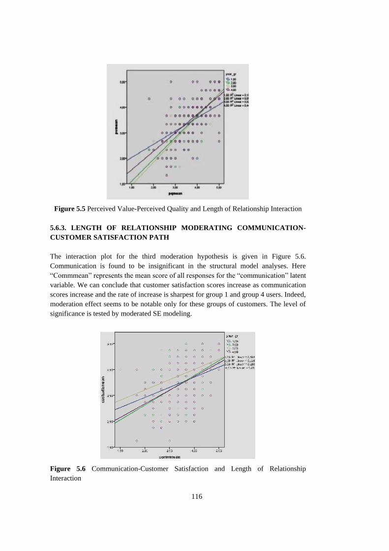
116

Figure 5.5 Perceived Value-Perceived Quality and Length of Relationship Interaction

5.6.3. LENGTH OF RELATIONSHIP MODERATING COMMUNICATION-

CUSTOMER SATISFACTION PATH

The interaction plot for the third moderation hypothesis is given in Figure 5.6.

Communication is found to be insignificant in the structural model analyses. Here

“Commmean” represents the mean score of all responses for the “communication” latent

variable. We can conclude that customer satisfaction scores increase as communication

scores increase and the rate of increase is sharpest for group 1 and group 4 users. Indeed,

moderation effect seems to be notable only for these groups of customers. The level of

significance is tested by moderated SE modeling.

Figure 5.6 Communication-Customer Satisfaction and Length of Relationship

Interaction

117

5.6.4. HOUSEHOLD’S INCOME LEVEL MODERATING SATISFACTION-

LOYALTY PATH

The interaction plot for the fourth moderation hypothesis is given in Figure 5.7.

Household’s Income Level is found to be insignificant in the extended SEM analyses.

Thus we have decided to explore its interaction effects. Household Income level is asked

as a six- category question. Then thoses responses are further re-coded to three groups

for ease of analysis as follows: gr_income=1 : Customers whose monthly income is below 1000 TL

gr_income=2 : Customers whose monthly income is between 1000 - 4500 TL

gr_income=3: Customers whose monthly income is higher than 4500 TL

We can conclude that loyalty scores increase as satisfaction scores increase and there is

no notable interaction between the three variables. The level of significance is tested by

moderated SE modeling.

Figure 5.7 Satisfaction-Loyalty – Household Income Level Interaction Plot

5.6.5. HOUSEHOLD’S INCOME LEVEL MODERATING PERCEIVED

QUALITY PERCEIVED VALUE PATH

The interaction plot for the fifth moderation hypothesis is given in Figure 5.8. We can

conclude that perceived value scores increase as perceived quality scores increase and

the interaction effect is mostly notable for Group 1 users. The level of significance is

tested by moderated SE modeling.

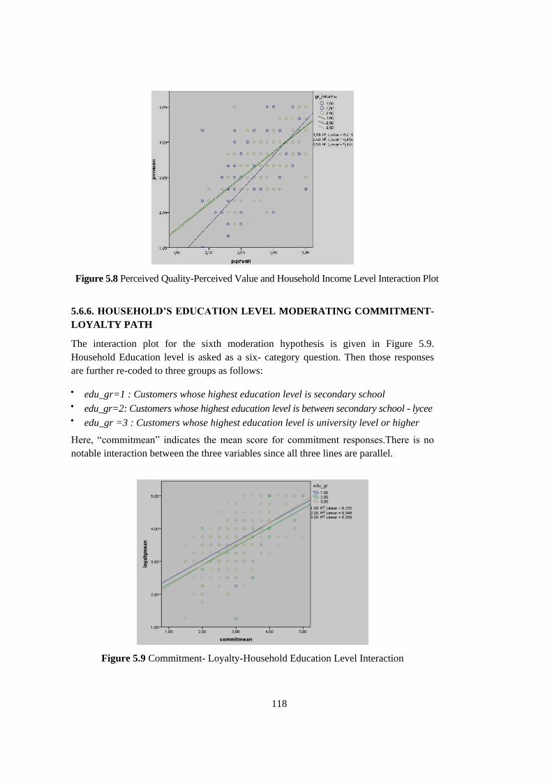
118

Figure 5.8 Perceived Quality-Perceived Value and Household Income Level Interaction Plot

5.6.6. HOUSEHOLD’S EDUCATION LEVEL MODERATING COMMITMENT-

LOYALTY PATH

The interaction plot for the sixth moderation hypothesis is given in Figure 5.9.

Household Education level is asked as a six- category question. Then those responses

are further re-coded to three groups as follows:

edu_gr=1 : Customers whose highest education level is secondary school

edu_gr=2: Customers whose highest education level is between secondary school - lycee

edu_gr =3 : Customers whose highest education level is university level or higher

Here, “commitmean” indicates the mean score for commitment responses.There is no

notable interaction between the three variables since all three lines are parallel.

Figure 5.9 Commitment- Loyalty-Household Education Level Interaction

119

5.6.7. HOUSEHOLD’S EDUCATION LEVEL MODERATING PERCEIVED

QUALITY-PERCEIVED VALUE PATH

The interaction plot for the sixth moderation hypothesis is given in Figure 5.10. We can

conclude that perceived value scores increase as perceived quality scores increase and

the interaction effect is mostly notable for Group 1 users. The level of significance is

tested by moderated SE modeling.

Figure 5.10 Perceived Quality-Perceived Value and Household Education Level

Interaction Plot

5.6.8. MODERATION EFFECTS TESTED BY SPSS PROCESS MACRO

We have used SPSS PROCESS tool (Hayes, 2012) to test moderation loop structures.

We use Model 4 template which is the basic moderation model in the software’s

templates. The results are as follows (N denotes insignificant effect):

Length of Relationship moderates the relation between customer satisfaction and

loyalty (N)

Length of Relationship moderates the relation between Perceived quality and

perceived value. (N)

Length of Relationship moderates the relation communication and customer

satisfaction. (N)

Household’s Income Level moderates relation between customer satisfaction and

loyalty. (N)

Household’s Income Level moderates relation between perceived quality and

perceived value.

Household’s Education Level moderates the relation between commitment and

loyalty. (N)

Household’s Education Level moderates the relation between perceived quality and

perceived value.

120

The above results give more precise results than interaction plots since they consider the

overall data within a regression framework.

5.6.9. MODERATION EFFECTS TESTED BY INTERACTION MODELS

Based on the prior moderation analyses, we have carried out moderated SEM analyses

with our data to test hypothesized interaction relations.

5.6.9.1. THE METHOD

Moderation effects are tested by using mean-centered products of the indicators of the

exogenous latent variables and covariate variables.

A generic interaction model is developed by Kenny and Judd (1984) as follows. Here the

endogenous variable η is caused by two exogenous variables, ξ1, ξ2, and one interaction

latent variable ξ3.

Figure 5.11 A Moderated SEM (Kenny and Judd, 1984)

Our suggested interaction model is given below. This model shows the interaction effect

of “length of relationship” (“year” in the diagram) on the “perceived quality - perceived

value” relationship. The interaction latent variable is shown by the “year x pv” circle

and its indicators (V42, V43 and V44) are obtained as the products of “year” indicator

with the three indicators of perceived quality. Thus three possible combinations are

formed by taking the products of mean-centered values for each measured variable.

121

Figure 5.12 Our Moderation Model for a Hypothesized Path

We have adapted the above model with the “unconstrained approach” as suggested by

Marsh and Hau (2006 cited by Hancock, 2012, personal communications in 2013). In

this approach, the products of observed variables are used to form the indicators of the

composite (product) latent variables. There are no other constraints imposed and

simulation results have shown that the method yields similar results as the constrained

approaches by other researchers and has performed better under non-normality

conditions as well. Our use of pseudo-latent variables has enabled us to use the

“unconstrained moderation approach” with covariates. Our sample data is non-normal

and that we prefer to use this method after review of application articles (Hancock,

2012, personal communications in 2013).

5.6.9.2. MODERATED STRUCTURAL MODELS

A moderated SEM is constructed for each hypothesis. The interaction effects are

imposed on covariate- extended structural models explained in section 5.4. Each

hypothesis is tested separately due to the increase in complexity. Each interaction adds

many degrees of freedom and also possible collinearity effects compared to adding a

single latent variable with many indicators. In each iteration, some fit indices worsened.

Goodness of Fit indices are reported to be biased when sample size is large relative to

degrees of freedom or biased upwards when sample size is small relative to degrees of

freedom (personal communications with E. Rigdon, 2013). Thus other fit indices are

checked to see models’ improvements. Since SEM allows a precise analysis of complex

relationships, the above hypotheses are all tested and further new ones are also added.

The working models and results are given below:

MODEL 1: BASE MODEL and A NEW INTERACTION HYPOTHESIS (length of

relationship moderates the relation between insensitivity and commitment)

122

MODELLING STEPS (BOLLEN, 1989):

1. Specification of the model: The model is specified with the latent variable

relationships and one additional moderation constraint. The interaction variable is

added as follows:

Commitment = insensitivity customer satisfaction length of relationship length x insensi.

The interaction variable is specified a variable with two new indicators. Those are

obtained as the products of mean-centered values of the indicators of insensitivity (2

indicators) and length of relationship (1 indicator) variables. This has resulted in two

possible combinations.

2. Implied Covariance Matrix: Is calculated based on the sample data measurements.

Software runs reveal the results.

3. Identification: The number of data points exceeds the number of parameters to be

estimated and thus the model is identified. If the model is not identified, then

estimation cannot be done and SEM software gives error messages.

4. Estimation: The loading values, R2 values, error variances and t-values are computed

and displayed successfully.

5. Testing and Diagnostics: The model fit values are tested after a preliminary set of

runs and modifications are made based on suggested item-error correlations and not

on suggested re-loadings.

6. Re-specification: In the first three runs, the model is re-specified with the addition of

item-error correlations until a set of satisfactory fit values are obtained.

ANALYSIS RESULTS:

The first iteration yielded poor fit and then by letting items freely correlate, the

necessary modifications are made. In the third run, a satisfactory fit is reached. The fit is

best possible (2 (372) = 1935.48, p = .000, RMSEA = .080, GFI = .84, AGFI = .81,

NNFI = .90, CFI = .51 and PGFI =0.72) and examination of differences show that the

model significantly improved.

The structural equations are given below (csatis indicates customer satisfaction, pv

indicates perceived value, year indicates length of relationship, educ indicates household

education level, cexpect indicates customer expectations, imgrepu indicates company

image/reputation, tcommit indicates commitment, pq indicates perceived quality,

yinsenco indicates the year-insensitivity- commitment moderation variable) :

csatis = 0.93×pv - 0.044×year + 0.077×educ, Errorvar.= 0.0041 , R² = 1.00

(0.052) (0.025) (0.021) (0.0029)

17.87 -1.79 3.58 1.42

cexpect = 1.00×imgrepu, Errorvar.= 0.0015 , R² = 1.00

123

(0.043) (0.0014)

23.29 1.09

tcommit = 0.34×csatis + 2.77×insensi - 0.027×year + 0.035×yinsenco, Errorvar.= 0.024

, R² = 1.00

(0.31) (0.32) (0.071) (0.087) (0.018)

1.09 8.59 -0.39 0.41 1.36

trust = 1.00×imgrepu, Errorvar.= 0.00 , R² = 1.00

(0.043) (0.0010)

23.08 0.061

loyalty = 0.31×tcommit + 0.025×year, Errorvar.= 0.00020, R² = 1.00

(0.013) (0.023) (0.0020)

23.32 1.08 0.10

insensi = 1.00×trust, Errorvar.= 0.0040 , R² = 1.00

(0.021) (0.0017)

48.45 2.33

pv = 0.94×pq + 0.035×year, Errorvar.= 0.0031 , R² = 1.00

(0.053) (0.021) (0.0018)

17.79 1.67 1.70

After examining the t-values, the significant relations are given below:

Customer satisfaction = 0.93×perceived value + 0.077× household educ. level, R² = 1.00

Customer expect. = 1.00× Company image / reputations, R² = 1.0

Commitment = 2.77×insensitivity to comp. off. - 0.027×year + 0.035×yinsenco, R² = 1.00

Trust = 1.00× Company Image / Rep., R² = 1.00

Loyalty = 0.31×commitment, R² = 1.00

Insensitivity to comp. off. = 1.00×trust, R² = 1.00

Perceived Value = 0.94×Perceived quality, R² = 1.00

124

The model’s t- values are given in Figure 5.13.

Figure 5.13 Moderation Model 1

125

MODEL 2: BASE MODEL and TWO NEW INTERACTION HYPOTHESES; household

income level moderates the relation between customer expectations and perceived value;

MODELLING STEPS (BOLLEN, 1989):

1. Specification of the model: The model is specified with the latent variable

relationships and two additional moderation constraints. The interaction variables are

added as follows:

Commitment = insensitivity customer satisfaction length of relationship length x insensi.

Perceived Value= Perceived Quality Length of Rel. Cust. Expec. income income × cust.

Expect

The interaction variables are specified as variables with new indicators. Those new

indicators are obtained as the products of mean-centered values of the indicators.

2. Implied Covariance Matrix: Is calculated based on the sample data measurements.

Software runs reveal the results.

3. Identification: The number of data points exceeds the number of parameters to be

estimated and thus the model is identified. If the model is not identified, then

estimation cannot be done and SEM software gives error messages.

4. Estimation: The loading values, R2 values, error variances and t-values are computed

and displayed successfully.

5. Testing and Diagnostics: The model fit values are tested after a preliminary set of

runs and modifications are made.

6. Re-specification: In the first three runs, the model is re-specified with the addition of

item-error correlations until a set of satisfactory fit values are obtained

ANALYSIS RESULTS:

The first iteration yielded poor fit and then by letting items freely correlate, the

necessary modifications are made. In the third run, a satisfactory fit is reached. The fit is

best possible (2 (372453) = 1989.498, p = .000, RMSEA = .073, GFI = .84, AGFI =

.81, NNFI = .50, CFI = .51 and PGFI =0.72). Further modifications led to identification

and comvergence problems.

After examining the t-values, the structural equations are given below. The insignificant

and significant values are reported simultaneously to shed light on future comparisons.

Customer satisf. = 0.29×perc. val. - 0.031×year, R² = 1.00

Cexpect = 1.00×company image/rep, R² = 1.00

Commitment = 1.28×customer satisf. + 1.85×insensitivity to comp off +

0.021×length of rel.+ 0.0032×length of rel x insens., R² = 1.00

Trust = 1.00×company image/rep, R² = 1.00

Loyalty = 0.32×commitment, R² = 1.00

126

Insensitivity to comp off = 1.00×trust, R² = 0.99

Perc. val. = 1.08×cexpect + 2.33×perc. qual. + 0.13×length of rel.+ 0.15×incexpperc.

val. + 0.019× Household income, R² = 1.00

The model’s t- values are given in Figure 5.14.

Figure 5.14 Moderation Model 2

127

5.6.10. DIRECT AND INDIRECT EFFECTS OF MARKER ITEMS

The above results can all be compiled to give concrete meanings of structural effects of

consumer perceptions. We can embed the structural equations into the measurement

equations to derive the prediction models. We can use the marker items of latent variables as

“representative response items”. Strategic results of the derived equations are interpreted in

Chapter 6.

For moderation effects, the measurement items are created as interaction variables and for

the rationale of moderation, these effects will then be calculated based on the partial

derivatives of product terms.

The response-based measurement equations and their interpretations are listed below:

I) CUSTOMER SATISFACTION- DIRECT EFFECTS

V9= 0.60×0.29× V15 / 0.75

V9 = 0.232× V15

INTERPRETATION:

One unit increase in perceived value response will result in 0.232 units increase in customer

satisfaction response.

CUSTOMER SATISFACTION – INDIRECT EFFECTS

V9= 0.60×0.29×2.33× V13/0.82 +0.60×0.29×0.13×length of rel.+0.60×0.29×0.15×V45

V9=0.49 V13+0.02 length of rel. + 0.02 V45

INTERPRETATIONS:

One unit increase in perceived quality response will result in 0.49 units increase in

customer satisfaction.

One month’s increase in AC device usage will result in 0.02 unit increase in customer

satisfaction response.

II) CUSTOMER EXPECTATION- DIRECT EFFECTS

V20 = 0.73×1×V38 / 0.82

V20= 0.89 V38

128

INTERPRETATION:

One unit increase in company image response will result in 0.89 unit increase in customer

expectations response.

III) COMMITMENT- DIRECT EFFECTS

V24 = 0.62×1.28 × V9/0.6 + 0.62×1.85×V37/0.68

V24= 1.32 V9 + 1.68 V37

INTERPRETATIONS:

One unit increase in customer satisfaction response will result in 1.32 units increase in

commitment response.

One unit increase in insensitivity response will result in 1.68 units increase in

commitment response.

IV) TRUST- DIRECT EFFECTS

V29 = 0.79× V38 /0.82

V29= 0.98 V38

INTERPRETATION:

1 unit increase in company image response will result in 0.96 unit increase in trust response.

V) LOYALTY- DIRECT AND INDIRECT EFFECTS I

V32= 0.75×0.32×1.28×V9 /0.60 +0.75×0.32×1.85×V37/0.68

V32= 0.51 V9 + 0.65V37

INTERPRETATIONS:

One unit increase in customer satisfaction response will result in 0.51 unit increase in

loyalty response.

One unit increase in insensitivity response will result in 0.65 unit increase in loyalty

response.

129

LOYALTY- DIRECT AND INDIRECT EFFECTS II

V32 = 0.75×0.32×1.28×0.29×V15 / 0.75 + 0.32×1.85× V29 /0.79

V32 = 0.51 V15 + 0.75 V29

INTERPRETATIONS:

One unit increase in perceived value response will result in 0.51 unit increase in loyalty

response.

One unit increase in trust response will result in 0.749 unit increase in loyalty response.

VI) PERCEIVED VALUE- DIRECT AND INDIRECT EFFECTS

V15= 0.75×2.33×V13/0.82+0.75×0.13×length of relationship +0.75×0.15 ×incexpperc.val

V15= 2.3 V13 + 0.09 lengt of relationship + 0.11 interaction

INTERPRETATION:

1 unit increase in perceived quality response will result in 2.13 units increase in perceived

value response.

1 month’s increase in AC device usage will result in 0.09 unit increase in perceived value

response.

VII) PERCEIVED VALUE – EFFECT OF INTERACTION (income affecting

expectations- perceived value relationship)

V15= … +0.75×0.15 V46 (V46 being the marker composite indicator of interaction

variable)

V15= … + 0.112 V46

INTERPRETATION:

1 unit increase in income and 1 unit increase in customer expectations response will affect

the perceived value by 0.112 units.

VII) INSENSITIVITY TO COMPETITORS- DIRECT EFFECTS

V37= 1 × V29/0.79

V37= 1.265 V29

INTERPRETATION:

One unit increase in trust response will result in 1.265 units increase in insensitivity

response.

130

131

CHAPTER 6

STRATEGIC IMPLICATIONS AND FUTURE RESEARCH DIRECTIONS

6.1. AIM OF THE STUDY

The aim of this study is to provide empirical results on consumer attitudes for durable

goods. Several factors affecting customer satisfaction and loyalty are analyzed.

Interaction effects of covariates are modeled using moderation approaches. We aim to

provide directions for customer relationship and customer satisfaction measurement

strategies for air-conditioner manufacturers and retailers. Strategy recommendations to

manufacturers are provided in the report.

6.2. SUMMARY OF OUR FINDINGS AND STRATEGY RECOMMENDATIONS

6.2.1. DEVELOPING SURVEYS TO MEASURE CONSUMER ATTITUDES

NUMBER OF PERCEPTION VARIABLES

Our findings indicate that nine groups of customer perception variables are adequate to

measure customer satisfaction and loyalty for AC products. These are:

Satisfaction

Loyalty

Commitment

Trust

Perceived Quality

Perceived Value

Customer Expectations

Insensitivity to Competitive Offerings

Company Image/Reputation

NUMBER OF QUESTIONS

To achieve the best results, each perception variable can be measured by at least two or

three questions.

132

6.2.2. CONSUMER RESPONSES ON LENGTH OF UTILIZATION OF AN AC

PRODUCT

Our findings indicate that:

Customer satisfaction is affected by length of use of an AC product. The effect

becomes significant after three years’ of utilization.

The highest degree of loyalty is observed for long-term users (users of a product of

more than 3 years).

Commitment is studied as a predecessor of loyalty in our research. The highest degree

of commitment is observed for medium term (2-3years) consumers. Loyal customers

do not always display commitment attitudes.

Customer Expectations are best reported for medium term users (1- 2 years).

Insensitivity to Competitive Offerings is not affected by product experience. Thus we

cannot say that loyal or committed customers are not responsive to new product

campaigns of competitors.

Trust is not affected by level of product experience. Thus more experienced users do

not necessarily display higher levels of trust in brand or product.

Quality perception is highest for medium term users (2-3 years).

Value perception increases with level of product experience.

Company Image (brand) perception is not affected by level of product experience.

STRATEGY RECOMMENDATIONS TO MANUFACTURERS:

Loyalty campaigns should be addressed to long-term consumers.

Medium- term users should be informed of new and similar products to

strengthen commitment to the brand.

Quality research should be disseminated to all consumers and primarily to

medium- term users.

6.2.3. CONSUMER RESPONSES BASED ON HOUSEHOLD INCOME LEVEL

The responses are classified as to the household’s income level as follows:

Low-income users: Users with less than 4500 TL monthly income

High-income users: Users with more than 4500 TL monthly income

Our findings indicate that:

Customer expectations attain their highest values for high-income users.

Customer satisfaction or customer loyalty are not affected by household’s income

level.

133

6.2.4. CONSUMER RESPONSES BASED ON SIMULTANEOUS EFFECTS OF

LENGTH OF UTILIZATION AND HOUSEHOLD INCOME LEVEL

Responses are classified and analyzed based on household income levels and length of

use simultaneously.

Our findings indicate that:

Long-term consumers with higher income levels show higher levels of commitment.

STRATEGY RECOMMENDATION TO MANUFACTURERS:

Long-term consumers with higher income levels should be informed of new and

similar products to strengthen commitment to the brand.

6.2.5. CONSUMER RESPONSES BASED ON LENGTH OF UTILIZATION AND

HOUSEHOLD EDUCATION LEVEL

Our findings indicate that:

Long-term consumers with higher education levels show higher levels of commitment.

STRATEGY RECOMMENDATION TO MANUFACTURERS:

Long-term consumers with higher education levels should be informed of new and

similar products to strengthen commitment to the brand.

6.3. CONSUMER PERCEPTIONS AND FUTURE RESEARCH DIRECTIONS

6.3.1. CONSUMERS’ SATISFACTION WITH A PRODUCT

Our findings indicate that:

Customer satisfaction is positively affected by:

Value Perception

Consumers’ education level

Customer satisfaction is negatively affected by:

Length of Use of a Product

134

INTERPRETATION

Longer use of an AC device results in decrease in customer satisfaction. This can be

due to wish to change the product, consumers’ observations and their unmet

expectations.

Better- educated consumers can perceive an AC product’s performance better and

thus have higher levels of satisfaction.

FUTURE RESEARCH DIRECTIONS

Effect of “Length of relationship” can be studied for other durable goods or expensive

services.

Effect of “Household Education Level” can be studied for other durable goods or

expensive services.

6.3.2. CONSUMERS’ LOYALTY TO A PRODUCT / BRAND

Our findings indicate that:

Customer loyalty is positively affected by:

Commitment

Length of Use of a Product

INTERPRETATION

Longer use of an AC device results in elevated loyalty.

More committed customers show higher levels of loyalty. Thus commitment is equally

important for residential AC users as business users of other products or services.

FUTURE RESEARCH DIRECTION

Commitment- loyalty relationship can be studied for other groups of durable goods

and different types of services.

6.3.3. CONSUMERS’ EXPECTATIONS FROM A PRODUCT/BRAND

Our findings indicate that:

Consumers’ expectations are positively affected by:

Company Image / Brand Reputation.

135

INTERPRETATION

Brand perception is the only factor affecting consumers’ expectations from a product.

FUTURE RESEARCH DIRECTION

Brand perception- expectations link can be studied for other groups of durable goods

and different types of services.

6.3.4. CONSUMERS’ TRUST IN A PRODUCT/BRAND

Our findings indicate that:

Consumers’ trust is positively affected by:

Company Image / Brand Reputation.

INTERPRETATION

Brand perception is the only factor affecting consumers’ trust in a brand / product.

FUTURE RESEARCH DIRECTION

Brand perception- trust can be studied for other groups of durable goods and different

types of services.

6.3.5. CONSUMERS’ INSENSITIVITY TO COMPETITIVE OFFERINGS

Our findings indicate that:

Consumers’ Insensitivity To Competitive Offerings is positively affected by:

Trust In a brand / product

INTERPRETATION

Brand / product trust is the only factor affecting Consumers’ Insensitivity To

Competitive Offerings.

FUTURE RESEARCH DIRECTION

Brand trust- switching attitudes can be studied for other groups of durable goods

and different types of services.

136

6.3.6. CONSUMERS’ VALUE PERCEPTION FOR AN AC PRODUCT

Our findings indicate that:

Consumers’ value perception is positively affected by:

Quality perception of a product

Consumers’ quality perception - value perception relation is strengthened by the

effect of “household income level” of a product.

INTERPRETATION

Quality perception is the only factor affecting Consumers’ value perception.

Quality perception has an indirect effect on consumer satisfaction.

Quality perceptions of consumers with higher income levels have stronger effects on

their value perceptions.

FUTURE RESEARCH DIRECTIONS

Brand trust- switching attitudes relationship can be studied for other groups of

durable goods and different types of services.

Quality perception- customer satisfaction relationship can be studied for other

groups of durable goods and different types of services.

Quality perception- value perception- household income level relationship can be

studied for can be studied for other groups of durable goods and different types of

services with larger samples.

6.3.7. CONSUMERS’ COMMITMENT TO A PRODUCT/BRAND

Our findings indicate that:

Consumers’ commitment is positively affected by:

Their insensitivity to competitive offerings.

Consumers’ commitment is strengthened by the effect of “length of use” of a

product.

Consumers’ commitment is positively affected by consumers’ satisfaction under the

effect of “length of relationship” variable.

Consumers’ commitment is more affected by their insensitivity to competitive

offerings under the effect of “length of relationship” variable.

INTERPRETATION

Switching attitudes of consumers affects their commitment to a brand /product.

Switching attitudes of consumers indirectly affect their loyalty to a brand/product.

137

Long- term users display more commitment with increasing levels of satisfaction.

Length of use of a product increases the effect of switching attitudes on commitment

attitudes.

FUTURE RESEARCH DIRECTIONS

Commitment- switching attitudes relationship can be studied for other groups of

durable goods and different types of services.

Loyalty- switching attitudes can be studied for other groups of durable goods and

different types of services.

Commitment- length of relationship path can be studied for other groups of durable

goods and different types of services.

Moderating effect of length of relationship on customer satisfaction-commitment can

be studied for durable goods, services with larger samples.

6.4. RESPONSE PREDICTION FOR MARKETING STRATEGIES

Based on the structural equations obtained in Chapter 5, we can derive the following

detailed prediction strategies for consumer responses in repeated survey applications:

1 Unit increase in perceived value response will result in 0.232 units increase in

customer satisfaction response.

1 Unit increase in perceived quality response will result in 0.49 units increase in

customer satisfaction.

1 month’s increase in AC device usage will result in 0.02 unit increase in customer

satisfaction response.

1 unit increase in company image response will result in 0.89 unit increase in

customer expectations response.

1 unit increase in customer satisfaction response will result in 1.32 units increase in

commitment response.

1 unit increase in insensitivity response will result in 1.68 units increase in

commitment response.

1 unit increase in company image response will result in 0.96 unit increase in trust

response.

1 unit increase in customer satisfaction response will result in 0.51 unit increase in

loyalty response.

1 unit increase in insensitivity response will result in 0.65 unit increase in loyalty

response.

1 unit increase in perceived value response will result in 0.51 unit increase in loyalty

response.

1 unit increase in trust response will result in 0.75 unit increase in loyalty response.

1 unit increase in perceived quality response will result in 2.13 units’ increase in

perceived value response.

138

1 month’s increase in AC device usage will result in 0.09 unit increase in perceived

value response.

1 unit increase in trust response will result in 1.265 units’ increase in insensitivity

response.

1 unit increase in income level and 1 unit increase in customer expectations response

will affect the perceived value response by 0.112 units.

6.5. ADDITIONAL FUTURE RESEARCH DIRECTIONS

MULTIGROUP SEM ANALYSES

We have studied “length of relationship” as a covariate in our research. This covariate

can also be added as a grouping variable in a SEM analysis for large samples. For smaller

samples, multi-group SE modeling is not possible. But for large samples, the covariate’s

effect can be studied for different groups of users. As we have given in Chapter 3, a

possible grouping strategy can be given as follows:

1. Customers in the first group are the “new” users of a good. They have been using the

product for at most one year.

2. Customers in the second group are the “relatively mature” users of a good. They have

been using the product for one to three years, three years being the generally accepted

warranty period for durable goods.

3. Customers in the third group are the “mature” users of a good. They have been using

the product for at least three years.

LONGITUDINAL SEM ANALYSES

There are distinct consumption phases for AC products or for durable products with

similar consumption characteristics. Thus, “length of use of a product” can be

incorporated into the problem or into a similar problem. Some or all of the latent

variables can be replicated over periods, which can be taken as “seasons” or “years”.

Thus a baseline SEM can be constructed and can further be extended to cover more than

one point in time. This is longitudinal modeling approach. Many measurement points

should exist for this type of a research.

139

REFERENCES

1. Aaker, David A., K. L. Keller (1990), "Consumer Evaluations of Brand Extensions,"

Journal of Marketing, 54 (January), pp. 27-41.

2. Aiken, Lewis R. (1985), "Three coefficients for analyzing the reliability and validity

of ratings." Educational and psychological measurement 45.1, pp.131-142.

3. Ainsworth, J.(2005), “PSY524 Lecture Notes Structural Equation Modeling”,

California State University, retrieved from http://www.csun.edu/~ata20315.

4. Akgözlü, T., Industry Expert in Alarko (2010-2013), Personal Communications.

5. Albaum, Gerald, (1997), "The Likert scale revisited", Journal of Market Research

Society, pp.331-348.

6. Alpar, R. (2010), Spor, Sağlık ve Eğitim Bilimlerinden Örneklerle Uygulamali

İstatistik Ve Geçerlik, Güvenirlik”, Detay Yayıncılık, Ankara.

7. Anderson E W, Fornell C., (2000), “Foundations of the American customer

satisfaction index”, Journal of Total Quality Measurement, 11(7), pp.869–882.

8. Anderson E. W., Sullivan M. W.(1993), “The Antecedents and Consequences of

Customer Satisfaction for Firms”, Marketing Science, (12), p.125–143.

9. Anderson, E.W., Fornell, C. and Lehmann, D.R. (1994), “Customer Satisfaction,

Market Share and Profitability: Findings From Sweden”, Journal of Marketing, Vol.

58, pp. 53-66.

10. Anderson, James C., and David W. Gerbing (1988), "Structural equation modeling in

practice: A review and recommended two-step approach", Psychological Bulletin

103.3, p. 411.

11. Andreassen, T.W., B. Lindestad, (1998), “Customer Loyalty and Complex Services”,

International Journal of Service Industry Management, Vol. 9, No.1, pp.7-23.

12. Antokanis, John (2011), SEMNET List Discussions.

13. Arıkan, S. (2010), Construct Validity and Factor Structure of Student Selection

Examination across Subgroups, Ph.D.Thesis in Mathematics Education METU,

retrieved from http://etd.lib.metu.edu.tr/upload/12611814/index.pdf.

14. Bagozzi, R.P., ed. (1994), Advanced Methods of Marketing Research, Blackwell

Publishers.

15. Ball, D., P.S. Coelho, A.Machas (2004), “The Role of Communication and Trust in

Explaining Customer Loyalty”, European Journal of Marketing, Vol.38, No.9/10, pp.

1272-1293.

16. Batmaz, İ., Professor in METU(2009-2013), Personal communications.

17. Bell, Simon J., Seigyoung Auh, and Karen Smalley (2005), "Customer relationship

dynamics: service quality and customer loyalty in the context of varying levels of

customer expertise and switching costs." Journal of the Academy of Marketing

Science 33.2, pp.169-183.

18. Bentler, R., (1980), “Multivariate Analysis with Latent Variables: Causal Modeling”,

Annual Review of Psychology, Vol. 31, pp. 419-456.

140

19. Bloemer J., K. Ruyter (1999), “Customer loyalty in high and low involvement service

settings: the moderating impact of positive emotions”, Journal of Marketing

Management, (15), pp. 315–330.

20. Bollen, K. (1989), Structural Equations with Latent Variables, New York, John

Wileyand Sons, Inc.

21. Bollen, K. and J. Brand (2008), “Fixed and Random Effects in Panel Data Using

Structural Equations Models”, California Center for Population Research On-Line

Working Paper Series.

22. Bollen, K.A., S. Bauldry, (2011), “Three Cs in measurement models: Causal

indicators, composite indicators, and covariates”, Psychological Methods, Vol 16(3),

pp. 265-284.

23. Bolton, R.N., K.N. Lemon and P. C. Verhoef (2008), “Expanding Business-to-

Business Customer Relationships: Modeling the Customer’s Upgrade Decision”,

Journal of Marketing, Vol. 72, pp.46–64.

24. Bontis, N, Booker, L. and A. Serenko. (2007), “The mediating effect of organizational

reputation on customer loyalty and service recommendation in the banking industry”,

Management Decision, 45, 9, pp. 1426-1445.

25. Bowen, John. T., Shiang-Lih Chen (2001), “The Relationship between Customer

Loyalty and Customer Satisfaction”, International Journal of Contemporary

Hospitality Management, pp. 213-217.

26. Brown, S.W. and Bond, E.U. III (1995), "The internal/external framework and service

quality: Toward theory in Services Marketing", Journal of Marketing Management,

February, pp. 25-39.

27. Brown, T. J., Barry, T. E., Dacin, P. A., and Gunst, R. F. (2005), "Spreading the word:

Investigating antecedents of consumers’ positive word-of-mouth intentions and

behaviors in a retailing context." Journal of the Academy of Marketing Science 33.2,

pp. 123-138.

28. Brucks, M., V.A. Zeithaml, G. Naylorarie (2000), “Price and Brand Name As

Indicators of Quality Dimensions for Consumer Durables”, Journal of the Academy of

Marketing Science, Volume 28, No. 3, pp. 359-374.

29. Bruner, G. C., Hensel, P. J. and James, K. E. (2009), Marketing Scales Handbook,

American Marketing Association.

30. Burkholder, G., L. Harlow (2009), “An Illustration of a Longitudinal Cross-Lagged

Design for Larger Structural Equation Models”, Structural Equatıon Modelıng, 10(3),

pp. 465–486.

31. Caruana, A., and Ewing, M. T. (2010),”How corporate reputation, quality, and value

influence online loyalty”, Journal of Business Research, 63, 9-10, pp. 1103-1110.

32. Caruana, A., Money, A. H., and Berthon, P. R. (2000), “Service quality and

satisfaction–the moderating role of value”, European Journal of Marketing, 34(11/12),

pp. 1338-1353.

33. Cass Ngo O'Cass, Aron, and Liem Viet Ngo (2011), "Achieving customer satisfaction

in services firms via branding capability and customer empowerment." Journal of

Services Marketing 25.7, pp.489-496.

141

34. Čater, T. and Čater, B. (2010), “Product and relationship quality influence on

customer commitment and loyalty in B2B manufacturing relationships”, Industrial

Marketing Management, 39(8), pp.1321-1333.

35. Chiao, Y. C., Chiu, Y. K., and Guan, J. L. (2008), "Does the length of a customer–

provider relationship really matter?" The Service Industries Journal, 28.5 (2008),

pp.649-667.

36. Chiou, J.S. (2004), “The antecedents of consumer’s loyalty towards Internet service

providers”, Information & Management, Vol. 41, No. 6, pp. 685-695

37. Christensen, H., A.F. Jorn, A.J. Mackinnon, A.E. Korten, P.A. Jacomb, A.S.

Handerson and B. Rodgers, (1998), “Age differences in depression and anxiety

symptoms: a structural equation modelling analysis of data from a general population

sample”, Psychological Medicine, 29, pp. 325-339.

38. Churchill, G.A. (1979), “A paradigm for developing better measures of marketing

constructs”, Journal of Marketing Research (pre-1986), February issue, pp.64-73.

39. Coelho, P. S., and Esteves, S. P. (2007), “The choice between a five-point and a ten-

point scale in the framework of customer satisfaction measurement”, International

Journal of Market Research, 49(3), pp.313-339.

40. Coltman, T., T.M. Devinney, D.F. Midgley and S. Venaik (2008), “Formative versus

reflective measurement models: Two applications of formative measurement”, Journal

of Business Research, 61(12), pp. 1250-1262.

41. Cortina, J. M., Chen, G., and Dunlap, W. P. (2001), “Testing interaction effects in

LISREL: Examination and illustration of available procedures”, Organizational

research methods, 4(4), pp. 324-360.

42. Coşkun, N., Dr., Bilkent University (2009-2013), Personal Communications.

43. Cox III, E. P. (1980), “The optimal number of response alternatives for a scale: A

review”, Journal of Marketing Research, pp. 407-422.

44. Cronin Jr, J. J., Brady, M. K., & Hult, G. T. M. (2000), “Assessing the effects of

quality, value, and customer satisfaction on consumer behavioral intentions in service

environments”, Journal of retailing, 76(2), 193-218.

45. Davidian, M. (2007), Applied Longitudinal Data Analysis Lecture Notes, North

Carolina State University, retrieved from www4.stat.ncsu.edu/~davidian.

46. Davis-Sramek, Beth, John T. Mentzer and Theodore P. Stank (2008), “Creating

Consumer Durable Retailer Customer Loyalty through Order Fulfillment Service

Operations,” Journal of Operations Management, Vol. 26, No. 6, pp. 781-797.

47. Day, G.S. (1969), ``A two-dimensional concept of brand loyalty'', Journal of

Advertising Research, Vol. 9 No. 3, pp. 29-35.

48. De Lange, A.,T. W. Taris, I. L. D. Houtman, Michiel A. J.(2003), “ “The Very Best of

the Millennium”: Longitudinal Research and the Demand-Control-(Support) Model”,

Journal of Occupational Health Psychology, Vol. 8, No. 4, pp. 282–305.

49. De Matos, Celso Aususto, Rossi, C.A.V., Veiga, R.T., and Voeira, V.A. (2009),

“Consumer reaction to service failure and recovery: the moderating role of attitude

toward complaining”, Journal of Service Marketing, 23(7), pp. 462-475.

50. Diamantopoulos A. (1999) “Viewpoint: Reflective versus Formative Indicators”,

International Marketing Review 1999; 16 (6): 444-457.

142

51. Diamantopoulos, A., P.Riefler, K.P.Roth (2008), “Advancing Formative Measurement

Models”, Journal of Business Research, 61, pp. 1203–1218.

52. Dick, A.S. and Basu, K. (1994), “Customer loyalty: toward an integrated conceptual

framework”, Journal of the Academy of Marketing Science, Vol. 22, pp. 99-113.

53. Diggle, P., P. J. Heagerty, S. L. Zeger (2002), Analysis of Longitudinal Data, Second

Ed., Oxford University Press.

54. Duman, T (2003), “Kruvaziyer (Gemi) Turları Satın Alan Tüketicilerin Geleceğe

Yönelik Davranişsal Eğilimlerini Etkileyen Faktörlerin Yapisal Eşitlik Modeli İle

İncelenmesi”, Balikesir Üniversitesi Sosyal Bilimler Dergisi, pp.160-177.

55. Eaton, W. (2006), “Statistics for Psychosocial Research Lecture Notes”, Johns

Hopkins Bloomberg School of Public Health, retrieved from

ocw.jhsph.edu/courses/statisticspsychosocialresearch/PDFs/Lecture3.pdf.

56. Ekici, A., Assistant Professor in Bilkent University (2012,2013), Personal

communications.

57. Erdem, R., S. Rahman, L.Avcı, B. Demrel, S. Köseoğlu, G. Fırat, T. Kesici, S.

Kırmızıgül, S. Uzel, C. Kubat(2008), “ Hasta Memnuniyetinin Hasta Bağlılığı Üzerine

Etkisi”, Erciyes Üniversitesi İİBF Dergisi, S.31, pp. 95-110.

58. Fan, X., Thompson, B., & Wang, L. (1999), “Effects of sample size, estimation

methods, and model specification on structural equation modeling fit indexes,

Structural Equation Modeling: A Multidisciplinary Journal, 6(1), 56-83.

59. Farrell, A.(1994), “Structural Equation Modeling with Longitudinal Data: Strategies

for Examining Group Differences and Reciprocal Relationships”, Journal of

Consulting and Clinical Psychology. Vol.62 (3), pp. 477-487.

60. Ferron, J.M., M.R. , Hess (2007), “Estimation in SEM: A Concrete Example” , journal

Of Educational And Behavioral Statistics, vol. 32 no. 1, pp. 110-120.

61. Flavian, C. and Guinaliu, M. (2006), “Consumer trust, perceived security and privacy

policy: three basic elements of loyalty to a web site”, Industrial Management and Data

Systems, Vol. 106 No. 5, pp. 601-620.

62. Fornell, Claes, Michael D. Johnson, Eugene W. Anderson, Jaesung Cha, and Barbara

Everitt Bryant (1996), "The American Customer Satisfaction Index: Nature, Purpose,

and Findings," Journal of Marketing, 60 (4), pp. 7-18.

63. Fullerton, G.(2011), “Creating advocates: The roles of satisfaction, trust and

commitment”, Journal of Retailing and Consumer Services, Volume 18, Issue 1, pp.

92–100.

64. Garbarino E., M. S. Johnson (1999), “The different roles of satisfaction, trust, and

commitment in customer relationships”, Journal of Marketing, 63, pp. 70–87.

65. Garrett-Meyer, Elizabeth (2006), “Statistics for Psychosocial Research Lecture

Notes”, Johns Hopkins Bloomberg School of Public Health, retrieved from

ocw.jhsph.edu/courses/statisticspsychosocialresearch/PDFs/Lecture9.pdf.

66. Garson, D. (2010), Quantitative Research in Public Administration Lecture Notes,

North Carolina State University, retrieved from http://faculty.chass.ncsu.edu/garson

/PA765/index.htm.

143

67. Garvin, D.A. (1987), "Competing on the eight dimensions of quality", Harvard

Business Review, retrieved from cc.sjtu.edu.cn/G2S/eWebEditor/uploadfile/2013042

7091849944.pdf

68. Graham, J. (2009), “Missing Data Analysis: Making It Work in the Real World”,

Annual Review of Psychology, 60, pp.549–576.

69. Green, S., S. Marilyn (2006),” Structural Equation Modeling for Conducting Tests of

Differences in Multiple Means”, Psychosomatic Medicine, 68, pp. 706-717.

70. Gürel, E, Assistant Professor in Bilkent University (2009-2013), Personal

Communications.

71. Hair, J. F., et al. (2010), Multivariate Data Analysis, 7th Pearson Prentice Hall, Upper

Saddle River.

72. Hallowell, R. (1996), “The relationships of customer satisfaction, customer loyalty,

and profitability: an empirical study”, International Journal of Service Industry

Management, pp. 27-42.

73. Hancock, Gregory (2012), “Interactions and Nonlinear Relations”, Lecture Notes,

University of Maryland, retrieved from www.education.umd.edu/EDMS.

74. Hannemann, R. (1999), Sociology 203 B Course Notes, retrieved from

faculty.ucr.edu/~hanneman/soc203b/lectures/identify.html.

75. Hardesty, D.M., W.O. Bearden (2004), “The use of expert judges in scale

development, Implications for improving face validity of measures of unobservable

constructs”, Journal of Business Research, vol. 57, Issue 2, pp. 98-107.

76. Hayduk, L. and Littvay, L. (2012), “Should researchers use single indicators, best

indicators, or multiple indicators in structural equation models?”, BMC Medical

Research Methodology, 12(1), pp.159.

77. Hayes, A. F. (2012), “PROCESS: A versatile computational tool for observed variable

mediation, moderation, and conditional process modeling [White paper]”, retrieved

from http://www.afhayes.com/ public/process2012.pdf

78. Hogan, S. J. Soutar, G. N. McColl-Kennedy, J. R. & Sweeney, J. C. (2011),

“Reconceptualizing professional service firm innovation capability: Scale

development”, Industrial Marketing Management, 40(8), pp.1264-1273.

79. Hooper, D., J. Coughlan, M. Mullen (2008), "Structural Equation Modelling:

Guidelines for Determining Model Fit", Articles : 2.

80. Hoyle, R. H. (1991), “Evaluating measurement models in clinical research:

Covariance structure analysis of latent variable models of self-conception”, Journal of

Consulting and Clinical Psychology, 59, pp. 67–76.

81. http://www.statmodel.com discussions.

82. Hunter, V.L. (1998), ``Measure customer loyalty for complete picture of ROI'',

Business Marketing, Vol. 83 No. 3, pp. 18.

83. Iacobucci, D. (2010), “Structural equations modeling: Fit indices, sample size, and

advanced topics”, Journal of Consumer Psychology, 20(1), pp. 90-98.

84. Jaccard, J. and Wan, C. K. (1995), “Measurement error in the analysis of interaction

effects between continuous predictors using multiple regression: Multiple indicator

and structural equation approaches”, Psychological Bulletin, 117(2), pp. 348-357.

144

85. Johnson M. D., Auh S. (1998), “Customer satisfaction, loyalty, and the trust

environment”, Advances in Consumer Research, 25, pp.15–20.

86. Jones T. O., Sasser E. W. (1995), “Why satisfied customers defect”, Harvard Business

Review, 73, pp.88–101.

87. Jöreskog, K. G., and Wang, F. (1996), “Nonlinear structural equation models: The

Kenny-Judd model with interaction effects”, Advanced Structural Equation Modeling:

Issues and Techniques, Lawrence Erlbaum Associates.

88. Kaplan, David (2000), Structural Equation Modeling, Foundations and Extensions,

Sage Publications.

89. Kavak, B. (2008), “Pazarlama ve Pazar Araştırmaları: Tasarım ve Analiz”, Detay

Yayıncılık, ANKARA.

90. Kavak, B. Professor in Hacettepe University (2012-2013), Personal communications.

91. Kenny, D. (2011), “Measuring model fit”, Lecture Notes, University of Maryland,

retrieved from http://davidakenny.net/cm/fit.htm.

92. Kenny, D. A., and Judd, C. M. (1984),”Estimating the nonlinear and interactive

effects of latent variables”, Psychological bulletin, 96(1), pp.201-210.

93. Kılınç, C. (2009), “Sağlık Sektöründe Faaliyette Bulunan Hastane İşletmelerinde

Müşteri İlişkileri Yönetimi Üzerine Bir Araştırma”, Review of Social, Economic and

Business Studies, Vol.9/10, s. 309-332.

94. Kline, R. B. (2011), “Principles and practice of structural equation modeling”,

Guilford Press.

95. Köksal, G, Professor in METU (2009-2013), Personal communications.

96. Kotler, P. (2000), Marketing Management, Prentice Hall, New Jersey.

97. Kotler, P. (2006), Marketing for Hospitality and Tourism, Pearson Education Inc.,

Upper Saddle River, New Jersey.

98. Kramer, G.H.(1983), “The Ecological Fallacy Revisited: Aggregate- versus

Individual-level Findings on Economics and Elections, and Sociotropic Voting”, The

American Political Science Review, Vol. 77, No. 1, pp. 92-111.

99. Kreynefeld, M. and R.Walke (2009), “Applied Event History Analysis”, Winter

2009/2010 Seminar, International Max Planck Research School for Demography,

retrieved from http://www.imprs-demogr.mpg.de/courses/08ws/301.htm.

100. Krishnan, A. R. (2011), "Determinants of Customer Loyalty Factors and its Impact in

Consumer Durable White Goods Market in Chennai City, Tamilnadu-A Study." IJM

2.1, pp.15-29.

101. Kuo, Y., Wu, C. and Deng, W. (2009), “The relationships among service quality,

perceived value, customer satisfaction and post-purchase intention in mobile value-

added services”, Computers in human behavior, 25, pp. 887-896.

102. Kwang, Kim Jae, I. Jeong , J. Park, Y. Park, C. Kim and Tae-Ho Kim (2007), “The

impact of network service performance on customer satisfaction and loyalty: high-

speed internet service case in Korea”, Expert Systems with Applications, 32(3),

pp.822-831.

103. La Barbera, P. and D. Mazursky (1983), “A longitudinal assessment of consumer

satisfaction/dissatisfaction: the dynamic aspect of the cognitive process”, Journal of

Marketing Research, Vol. 20, No. 4, pp. 393-404.

104. Lars G, Anne M., Kai K. (2000), “The relationship between customer satisfaction and

loyalty: cross-industry differences”, Total Quality Management, 11, pp.509–514.

145

105. Likert, R., (1932), “A technique for the measurement of attitudes”, Archives of

Psychology, Vol 22 140, 55. , quoted in Hair et.al. (2010).

106. Lin, H.H., Y.S.Wang (2006), “An examination of the determinants of customer loyalty

in mobile commerce contexts”, Information and Management, 43, pp. 271–282.

107. Lin, J.C, P. Hsieh (2011), “Assessing the Self-service Technology Encounters:

Development and Validation of SSTQUAL Scale”, Journal of Retailing 87, 2, pp.

194-206.

108. Little, R. J. A. (1998), “ A test of missing completely at random for multivariate data with

missing values”, Journal of the American Statistical Association,83, pp.1198 – 1202.

109. Little, T., N. A. Card, K. J. Preacher, E. McConnell (2009), “Modeling Longitudinal

Data from Research on Adolescence”, in Handbook of Adolescent Psychology, Eds:

R. M. Lerner, L. Steinberg, Third Edition, John Wiley and Sons.

110. Liu, Annie H., Mark P. Leach, and Kenneth L. Bernhardt (2005), "Examining

customer value perceptions of organizational buyers when sourcing from multiple

vendors", Journal of Business Research 58.5, pp.559-568.

111. Lozano, L, E.G.Cueto, J.Muniz (2008), “Effect of the Number of Response Categories

on the Reliability and Validity of Rating Scales”, Methodology, Vol. 4(2):73–79.

112. MacCallum, R. C., Browne, M. W., and Sugawara, H. M. (1996), “Power analysis and

determination of sample size for covariance structure modeling”, Psychological

methods, 1(2), pp.130.

113. Marsh, H. W., & Balla, J. (1994), “Goodness of fit in confirmatory factor analysis:

The effects of sample size and model parsimony”, Quality and Quantity, 28(2), pp.

185-217.

114. Marsh, H. W., Balla, J. R., & McDonald, R. P. (1988), “Goodness-of-fit indices in

confirmatory factor analysis”, Psychological Bulletin, 103, pp. 391-410.

115. Marsh, H. W., Wen, Z., & Hau, K. T. (2006), “Structural equation models of latent

interaction and quadratic effects”, Structural equation modeling: A second course,

225-265 cited by Hancock (2013).

116. Marsh, H. W., Wen, Z., and Hau, K. T. (2004), “Structural equation models of latent

interactions: evaluation of alternative estimation strategies and indicator construction”,

Psychological methods, 9(3), pp.275.

117. Matsueda, J. (2012), “Structural Equation Modeling” Lecture Notes, University of

Washington.

118. Mazzarol, T., J.C. Sweeny, G.N. Soutar (2008), “Exploring the Message

Characteristics of Word-of-Mouth: A Study in a Services Context”, Australian and

New Zealand Marketing Academy Conference 2008 Proceedings.

119. McArdle, J. J. (2009), “Latent Variable Modeling of Differences and Changes with

Longitudinal Data”, Annual Review of Psychology, 60, pp.577–605.

120. Mulaik, S. (2009), Linear Causal Modeling with Structural Equations, Chapman

Hall/CRC Publishers.

121. Muthen, B. (1983), “Latent Variable Structural Modeling with Categorical Data”,

Journal of Econometrics, 22, pp.43-65.

122. Muthen, B.(1984), “A General Structural Equation Model with Dichotomous, Ordered

Categorical and Continous Latent Variable Indicators”, Psychometrika, 49, pp.115-32.

146

123. Muthen, L.K. and B. O. Muthen (1998), “Mplus: The comprehensive Modeling

Program for Applied Research”, Muthen and Muthen, Los Angeles.

124. Netemeyer, Richard G., William O. Bearden, and Subhash Sharma, eds. (2003),

Scaling procedures: Issues and applications, SAGE.

125. Newsom, J. (2012), “USP 655-Advanced Data Analysis: Structural Equation

Modeling”, Course Notes, Portland State University, retrieved from

http://www.ioa.pdx.edu/newsom.

126. Nunnally, C., I.H.Bernstein (1994), Psychometric Theory, New York: McGraw- Hill,

referred to in Hardesty and Bearden (2004).

127. Oktay, Ş. Industry Expert in Alarko (2010-2013), Personal Communications.

128. Oliva, T. A., Oliver R., MacMillan, I. C. (1992), “A catastrophe model for developing

service satisfaction strategies”, Journal of Marketing, 56, pp.83–95.

129. Oliver, R. L. (1999), “Whence consumer loyalty?”, Journal of Marketing, 63, pp. 33–44.

130. Özer, G., S. Aydın(2004), “GSM Sektöründe Müşteri Sadakati, Memnuniyeti,

Değiştirme Maliyeti ve Güven Arasındaki İlişki”, İktisadi Ve İdari Bilimler Dergisi /

Journal Of Economics and Administrative Sciences, Cilt 18, Sayı 3-4.

131. Pakkan, A., Industry Expert in ECA (2010-2012), Personal Communications.

132. Parasuraman, A., B. Leonard and V.A. Zeithaml (1988), “SERVQUAL: A Multiple-

Item Scale For Measuring Consumer Perceptions of Service Quality”, Journal of

Retailing, 1988, 64, 1, pp. 12-40.

133. Paşamehmetoğlu, A., Assistant Professor in Özyeğin University (2009-2013),

Personal Communications.

134. Paxton, P. (2008), “Structural Equation Modeling Lecture Notes”, Ohio State University,

retrieved from http://www.powershow.com/view1/17d6f5-NjEyY/Structural_Equation_

135. Modeling_An_Overview_powerpoint_ppt_presentation.

136. Payne, A. and Frow, P. (2005), “A strategic framework for customer relationship

management”, Journal of Marketing, 167-176.

137. Pedersen, S.S., A.Yagensky, O.R.F.Smith, O.Yagenska, V. Shpak and J. Denollet

(2009), “Preliminary “Evidence for the Cross-Cultural Utility of the Type D

Personality Construct in the Ukraine”, International Journal of Behavioral Medicine,

16, pp.108–115.

138. Preston, C. C., & Colman, A. M. (2000), “Optimal number of response categories in

rating scales: reliability, validity, discriminating power, and respondent preferences”,

Acta Psychologica, 104, pp. 1-15.

139. Pritchard, M.P. and Howard, D.R. (1997), “The loyal traveler: examining a typology

of service patronage'', Journal of Travelers Research, Vol. 35 No. 4, pp. 2-11.

140. Pritchard, M.P., Howard, D.R. and Havitz, M.E. (1992), ``Loyalty measurement: a critical

examination and theoretical extension'', Leisure Sciences, Vol. 14, pp. 155-64.

141. Pynnonen, Seppo (2010), “Latent Variable Structural Equation Modeling”, Lecture

Notes, retrieved from http://lipas.uwasa.fi/~sjp/Teaching/sem/lectures/.

142. Ranaweera, C., J. Pradhu (2003), “The influence of satisfaction, trust and switching

barriers on customer retention in a continuous purchasing setting”, International

Journal of Service Industry Management, Vol. 14 No. 4, pp. 374-395.

143. Reichheld F F., (1996), The Loyalty Effect, Harvard Business School Press.

147

144. Reichheld F. F., Sasser E. W. (1990), “Zero defections: quality comes to services”,

Harvard Business Review, 68, pp. 105–111.

145. Rigdon, E., (1996), “The Form of SEMs”, retrieved from www2.gsu.edu.

146. Rovinelli, R. J., & Hambleton, R. K. (1977), “On the use of content specialists in the

assessment of criterion-referenced test item validity”, Dutch Journal for Educational

Research, 2, pp.49-60.

147. Roy, K.S., G. Butaney, B.Bhutaney (2009), “Examining The Effects of The Customer

Loyalty States On The Word of Mouth”, Pacific Asia Conference on Information

Systems 2009 Proceedings.

148. Russo, F., M.Mouchart, M. Ghins, Michel, G. Wunsch (2006), “Statistical modelling

and causality in the social sciences”, Discussion Paper 0601, Institut de Statistique,

Université Catholique de Louvain.

149. Sabiote, Estela Fernández, and Sergio Román (2009), "The Influence of Social Regard

on the Customer–Service Firm Relationship: The Moderating Role of Length of

Relationship." Journal of Business and Psychology 24.4, pp. 441-453.

150. SAS (2008), “Structural Equation Modeling and Path Analysis Using PROC TCALIS

in SAS 9.2”, retrieved from www2.sas.com/proceedings/forum2008/384-2008.pdf.

151. Scheer L.K., C.F. Miao, J. Garrett (2010), “Effects of supplier capabilities on

industrial customers’ loyalty: the role of dependence”, Journal of the Academy of

Marketing Science , Volume 38, Number 1, pp. 90-104.

152. Selnes, F. (1993), An Examination of the Effect of Product Performance on Brand

Reputation, Satisfaction and Loyalty", European Journal of Marketing, Vol. 27, issue

9, pp. 19 – 35.

153. Singh, Harkiranpal (2006), “The importance of customer satisfaction in relation to

customer loyalty and retention”, UCTI Working Paper WP-06-06.

154. Sivadas, E., J. L. Baker–Prewitt (2000), “An examination of the relationship between

service quality, customer satisfaction, and store loyalty”, International Journal of

Retail and Distribution Management, Vol. 28(2), pp. 73-82.

155. Sousa, V. and W. Rojjanasrirat (2011), “Translation, adaptation and validation of

instruments or scales for use in cross-cultural health care research: a clear and user-

friendly guideline”, Journal of Evaluation in Clinical Practice Volume 17, Issue 2, pp.

268–274.

156. Steinmetz, H., Davidov, E., and Schmidt, P. (2011), “Three approaches to estimate

latent interaction effects: Intention and perceived behavioral control in the theory of

planned behavior”, Methodological Innovations Online, 6(1), pp.95-110.

157. Suh, J., Yi, Y. (2006), "When brand attitudes affect the customer satisfaction-loyalty

relation: the moderating role of product involvement", Journal of Consumer

Psychology, Vol.16, pp.145-55.

158. Sümbüloğlu, K., and Sümbüloğlu, V. (2009), “Biyoistatistik”, Hatiboğlu, Ankara.

159. Te Peci, M. (1999), ``Increasing brand loyalty in the hospitality industry'',

International Journal of Contemporary Hospitality Management, Vol. 11 No. 5, pp.

223-229.

160. Tse, D.K., F. Nicosia, P.C. Wilton (1990), “Consumer Satisfaction as a Process”,

Psychology and Marketing, Vol. 7(3), pp. 178-194.

148

161. Tung, L. L. (2004), “Service quality and perceived value’s impact on satisfaction,

intention and usage of short message service (SMS)”, Information Systems, Frontiers,

6(4), 353-368.

162. Türk Müşteri Memnuniyeti Indeksi çalışmaları, KALDER, retreived from tmme.org.

163. TURKSTAT, Turkey Institue of Statistics, Research Reports (2007, 2008 2010, 2011,

2012), retrieved from statistics experts and from www.tuik.org.

164. Türkyılmaz, A. and C. Özkan (2007), “Development of a customer satisfaction index

model, an application to the Turkish mobile phone sector”, Industrial Management

and Data Systems, Vol. 107 No. 5, pp. 672-687.

165. Ülengin, F., O.Kabak, S.Önsel, B.Ülengin, E.Aktaş (2010), “A Problem-Structuring

Model for Analyzing Transportation–Environment Relationships”, European Journal

of Operational Research 200, pp.844-859.

166. Uysal, M, J.Williams, Y.Yoon (2005), “Ziyaretçi Memnuniyetini Ölçmede İfade Edici

(Expressive) Faktörlere Karşılık Destekleyici (Instrumental) Faktörler”, Turizm

Araştırmaları Dergisi, Cilt 16, Sayı 1, pp.93-97.

167. Walsh, G., Mitchell, V.-W., Jackson, P. R. and Beatty, S. E. (2009), “Examining the

Antecedents and Consequences of Corporate Reputation: A Customer Perspective”,

British Journal of Management, 20, pp.187–203.

168. Wang G., L. Jia (2007), “Market segmentation based on customer satisfaction-loyalty

links”, Frontiers of Business Research China, 1(2), pp. 211–221.

169. Wang, Chung-Yu, and Li-Wei Wu (2012), "Customer loyalty and the role of

relationship length" Managing Service Quality 22.1, pp.58-74.

170. Westland, J., C. (2010), “Lower bounds on sample size in structural equation

modeling”, Electronic Commerce Research and Applications, 9(6), pp.476-487.

171. Wolfinbarger, M. and M.C.Gilly (2003),”eTailQ: Dimensionalizing, Measuring, and

Predicting etail Quality’, Journal of Retailing 79(3), pp. 183–198.

172. Wong, A., Dean, A. and White, C.J. (1999), ``Customer behavioral intentions in the

hospitality industry'', Australian Journal of Hospitality Management, Vol. 6 (autumn),

pp.53-63.

173. Wright, S. (1921), “Correlation and Causation”, Journal of Agricultural Research,

Vol. XX, 7, pp. 557-585.

174. Wright, S. (1934), “The Method of Path Coefficients”, The Annals of Mathematical

Statistics, Vol. 5, No. 3, pp. 161-215.

175. Yağcı, M.İ., T. Duman (2006), “Hizmet Kalitesi - Müşteri Memnuniyeti İlişkisinin

Hastane Türlerine Göre Karşılaştırılması: Devlet, Özel ve Üniversite Hastaneleri

Uygulaması”, Doğuş Üniversitesi Dergisi, 7 (2), pp. 218-238.

176. Yang, Z., Peterson R. T. (2004), “Customer perceived value, satisfaction and loyalty:

the role of switching costs”, Psychology and Marketing, 21(10), pp. 799–822.

177. Yi, Y. (1990), “A Critical Review of Customer Satisfaction”, Review of Marketing,

4(1), pp.68-123.

178. Yieh, K., Y. Chiao and Y. Chiu (2007) “Understanding the Antecedents to Customer

Loyalty by Applying Structural Equation Modeling”, Total Quality Management and

Business Excellence, Volume 18, Issue 3.

149

179. Yılmaz, V., E. Çelik (2005), “Bankacılık Sektöründe Müsteri Memnuniyeti ve

Bankaya Bağlılık Arasındaki İlişkinin Yapısal Eşitlik Modelleriyle Araştırılması”,

VII. Ulusal Ekonometri ve İstatistik Sempozyumu Bildirileri.

180. Yılmaz, V., E. Çelik, B., Depren (2011), “Devlet ve Özel Sektör Bankalarındaki

Hizmet Kalitesinin Karşilaştirilmasi: Eskişehir Örneği”, Doğuş Üniversitesi Dergisi, 8

(2), pp. 234-248.

181. Yozgatlıgil, C., Assistant Professor in METU(2009-2013), Personal communications.

182. Yu, C.J., L.Wu, Y. Chiao, H. Tai (2005), “Perceived Quality, Customer Satisfaction,

and Customer Loyalty: the Case of Lexus in Taiwan”, Total Quality Management,

Vol. 16, No. 6, pp. 707–719.

183. Zaim, S., Turkyilmaz, A., Tarim, M., Ucar, B. and Akkas, O, (2010), “Measuring

customer satisfaction in Turk Telekom Company using structural equation modeling

technique”, Journal of Global Strategic Management, 7, pp. 89-99.

184. Zeithaml, V. A. (2000), “Service Quality, Profitability, and the Economic Worth of

Customers: What We Know and What We Need to Learn”, Journal of the Academy of

Marketing Science, 28, pp.67–85.

185. Zeithaml, V. A., L.L. Berry, A.Parasuraman (1988), “Communication and control

processes in the delivery of service quality”, The Journal of Marketing, Vol. 52, pp.

35-48.

186. Zeithaml, V. A., L.L. Berry, A.Parasuraman (1993), “The Nature and Determinants of

Customer Service”, Journal of the Academy of Marketing Science, Vol. 21, pp. 1-12.

150

151

APPENDIX A

THE QUESTIONNAIRE FORM

A.1. THE PAPER FORM

KLİMALAR İÇİN MÜŞTERİ MEMNUNİYETİ ANKETİ

SAYIN KATILIMCI,

Bu çalışma, ODTÜ Endüstri Mühendisliği Bölümü’nde, ODTÜ-BİLİMSEL ARAŞTIRMA

PROJELERİ FONU destekli olarak, doktora öğrencisi Ayşegül Altaban ve öğretim üyeleri

Prof. Dr. Gülser Köksal ve Yrd. Doç. Dr. Ceylan Yozgatlıgil tarafından yürütülmektedir.

Çalışmanın amacı, klima ürünleri için müşteri bağlılığını etkileyen faktörleri ve etkilerini

gösterecek bir modelin geliştirilmesi ve ileride bu ürünleri kullanan tüketicilere verilen

hizmet kalitesinin ve müşteri memnuniyetinin artırılmasını sağlamaktır. Bulgular, müşteri

davranış biçimlerini ve beklentilerini ortaya koyma maksatlı olup kesinlikle anketi yanıtlayan

kişi özelinde değerlendirme yapılmayacaktır. Bu nedenle isim, adres gibi kişisel bilgiler

sorulmamaktadır. Gelir düzeyi, klima kullanım süresi gibi bilgiler de yalnızca analizler için

kullanılacaktır. Bu sorulara verilecek cevaplar da çalışmamızın başarısı için çok önem

taşımaktadır. Toplanan veriler gizli tutulacak ve sadece bilimsel yayınlarda kullanılacaktır.

Çalışmamız, yaklaşık 15 dakika sürmektedir. Anket sorularını, deneyimlerinize ve

beklentilerinize dayanarak cevaplamanız beklenmektedir. Bu çalışmaya katıldığınız için

şimdiden teşekkür ederiz. Sorularınız ve geri bildirimleriniz için Ayşegül Altaban (Tel: 0312

290 5032; E-posta: aysegula@yahoo.com, altaban@bilkent.edu.tr) ile iletişim kurabilirsiniz.

152

Table A.1. The Questionnaire Form

153

Table A.1. The Questionnaire Form (Continued)

154

A.2. THE WEB FORM

We have prepared a web-based questionnaire form for online response collection. We

have used METUSURVEY web medium. Two response entry screens are given below:

Figure A.1. Web-based response entry screen 1 in METUSURVEY medium

Figure A.2. Web-based response entry screen 2 in METUSURVEY medium

155

A screen of completed responses is given in Figure A.3.

Figure A.3. Screen of Completed Responses in METUSURVEY medium

156

157

APPENDIX B

THE LIST OF LISREL (LINEAR STRUCTURAL

EQUATION MODELING) NOTATIONS

Newsom (2012) provided the full list of Greek letters used in naming variables in

structural equation models. These notations are also called LISREL (an acronym for

Linear Structural Relations) naming convention. The list is given in Table B.1.

Table B.1. LISREL SEM Naming Conventions (Newsom, 2012)

158

159

APPENDIX C

SPSS PROCESS OUTPUT FOR A MODERATION MODEL EXAMPLE

(Hayes, 2012)

The following path diagram displays moderation effect of household education level

on perceived quality- perceived value relationship. Each latent variable is reduced to a

measured variable by calculating their latent mean scores.

Figure C.1 Moderation Effect of Household Education on Perceived Quality–Perceived

Value Path

The following SPPS PROCESS (Hayes, 2012) output displays moderation effect for the

following model :

PROCESS Procedure for SPSS Release 2.041 ****************

Written by Andrew F. Hayes, Ph.D. http://www.afhayes.com

************************************************************************

Model = 1

Y = pvmean X = pqmean M = edu_regr Sample size : 291

160

Outcome: pvmean

Model Summary

R R-sq F df1 df2 p

,6946 ,4825 66,5508 3,0000 287,0000 ,0000

Model

coeff se t p LLCI ULCI

constant 3,5426 ,0343 103,2845 ,0000 3,4751 3,6101

edu_regr,0276,0722,3820 ,7028 -,1145 ,1697

pqmean ,7728 ,0582 13,2821 ,0000 ,6583 ,8873

int_1 -,2768 ,1217 -2,2748 ,0237 -,5164 -,0373

Interactions:

int_1 pqmean X edu_regr

************************************************************************

*

Conditional effect of X on Y at values of the moderator(s)

edu_regr Effect se t p LLCI ULCI

-,7560 ,9821 ,0996 9,8603 ,0000 ,7861 1,1781

,2440 ,7053 ,0699 10,0856 ,0000 ,5676 ,8429

Values for quantitative moderators are the mean and plus/minus one SD from mean.

Values for dichotomous moderators are the two values of the moderator.

****************ANALYSIS NOTES AND WARNINGS **********************

Level of confidence for all confidence intervals in output: 95,00

NOTE: The following variables are mean centered prior to analysis: pqmean edu_regr

161

APPENDIX D

LIST OF TECHNICAL TERMS

1. AC: Air-Conditioner Device

2. AGFI: Adjusted Goodness-of-Fit Index, it is a goodness-of-fit index.

3. AMOS: It is a SEM software package. It is used as a second major analysis tool in

our study. It works together with SPSS. It is a visual programming tool.

4. CFI: Comparative Fit Index, it is a goodness-of-fit index.

5. Confirmatory Factor Analysis (CFA): It is a SEM technique for confirming a theory

of potential relationships among indicator variables and latent variables. The main

question is how well the collected data fit the hypothesized item groupings. The items

are firstly grouped latent variables. The collected data is then used for measuring the

degree of fit between the hypothesized and the real groupings.

6. GFI: Goodness-of-Fit Index, it is a goodness-of-fit index.

7. Goodness-of–Fit Indices: These are SEM statistics of the compliance of the

hypothesized and actually fitted model based on the sample data.

8. Indicators (also referred to as measured variables / questions or items): These are the

data items pertaining to questions in the questionnaire. They are used to assess the

effects of latent variables on overall consumer perceptions.

9. Latent Variables (also called “latents”,”factors” or “constructs”): These are the

underlying variables of measured human perception. They are measured by indicator

variables.

10. LISREL: It is a software package that can be used for SEM. It is used as the major

analysis tool in our study. The name is an acronym for “Linear Structural Relations”.

In this study, both versions 8.51 and 8.8 are used.

11. Model Fit: The fit of a SEM model is the discrepancy between the actual data’s

covariance matrix and the hypothesized model’s calculated covariance matrix. A

good fitting model has the minimum possible difference in between the two values.

12. Modification Indices: These are SEM software’s suggestions on improving the

estimated model. They are based on the possible improvements in the model’s chi-

square fit index.

13. NFI: Normed Fit Index, it is a goodness-of-fit index.

14. NNFI: Non- Normed Fit Index, it is a goodness-of-fit index.

15. Reliability: Is commonly defined as the stability or repeatibility of a measurement

instrument.

16. RMR: Root mean square residual, it is a goodness-of-fit index.

162

17. RMSEA: Root Mean Square Error, it is a goodness-of-fit index.

18. Sample: It is the specific group of respondents in our study.

19. SE: Structural Equations

20. SPSS: It is a general purpose statistical software package. In this study, versions 15,

18 and 20 (PASW/SPSS) are used.

21. Structural Equation Modeling (SEM): It is the collection of statistical techniques to

examine multiple interdependencies of independent and dependent variables. It is the

major analysis tool in our study.

22. Test Instrument: It is the questionnaire applied.

163

CURRICULUM VITAE

PERSONAL INFORMATION

Surname, Name: Altaban, Ayşegül

Date of Birth: 6 July 1965

Phone: +90 506 595 68 76

E-mail: aysegula@yahoo.com, altaban@bilkent.edu.tr

EDUCATION

Degree Institution Year of Graduation

MS METU, Industrial Engineering 1990

BS METU, Industrial Engineering 1987

High School TED Ankara College 1982

WORK EXPERIENCE

Year

2000- Present

Place

Bilkent University, Ankara

Enrollment

Instructor 1999- 2000 UYTES Software Consultant

1997 - 1999 LIKOM Project Consultancy Systems Analyst

1996- 1997 METU Computer Engineering Part-time Instructor

1988- 1995 METU Industrial Engineering Research Assistant

PUBLICATIONS

1. Sepil, C. A. and Altaban, A. (1992), “A Polynomially Bounded Dual Simplex

Algorithm for Capacitated Minimum Cost Flow Problem”, in Combinatorial

Optimization, pp. 307-308, Springer, Berlin, Heidelberg.

2. F. Sezgin, A. Altaban, and A.S. İkinci (2009), Hidromek- Part I, Intellectual Capital

Report of Turkey and Case Studies, (edited by Barbara Baker), pp. 94-106., Siyasal

Kitabevi, Ankara.

3. F. Sezgin, A. Altaban, and A.S. İkinci (2009), Bimeks, Intellectual Capital Report of

Turkey and Case Studies, (Edited by Barbara Baker), pp. 209-210, Siyasal Kitabevi,

Ankara.