NASATechnical

Paper3203

1992

National Aeronautics and

Space Administration

Office of Management

Scientific and TechnicalInformation Program

Structural Deterministic

Safety Factors SelectionCriteria and Verification

V. Verderaime

George C. Marshall Space Flight Center

Marshall Space Flight Center, Alabama

https://ntrs.nasa.gov/search.jsp?R=19920010113 2018-06-16T22:08:53+00:00Z

Acknowledgments

The author is grateful to Dr. J. Blair for the support, encouragement, and guidance receivedduring this study, and especially for the opportunity to contribute to such a core technology

touching most flight hardware. The expert statistics support from M. Rheinfurth, loads commentsand data provided by W. Holland, and the meaningful critique on contents and presentation by R.

Ryan are appreciated.

TABLE OF CONTENTS

I. INTRODUCTION ............................................................................................................

II. SOURCES OF STRUCTURAL FAILURE .....................................................................

A. Failure Tree ...............................................................................................................B. Data Evaluation .........................................................................................................

C. Prediction Uncertainties .............................................................................................

D. Discontinuities ............................................................................................................

E. Limits of Analysis ......................................................................................................

HI. PROBABILISTIC SAFETY INDEX ..............................................................................

A. Basic Probabilistic Concept .......................................................................................

B. Designing With Reliability .......................................................................................

C. Safety Index Sensitivities ..........................................................................................

IV. DETERMINISTIC SAFETY FACTOR ........................................................................

A. Safety Factor Concept ................................................................................................

B. Correlation With Probabilistic Safety ........................................................................

C. Safety Sensitivities ...................................................................................................

D. Safety Factors Selection Criterion ...........................................................................

E. Applied Stress Split Safety Factor ...........................................................................

V. SAFETY VERIFICATION .............................................................................................

A. Test Article Requirements .......................................................................................

B. Safety Data Interpretations .......................................................................................

VI. HUMAN FACTOR .........................................................................................................

VII. SUMMARY .....................................................................................................................

REFERENCES ........................................................................................................................

APPENDIX ..............................................................................................................................

Page

1

2

4

14

16

17

17

17

20

20

22

22

25

2630

32

33

3435

36

36

39

41

,°°

111

LIST OF ILLUSTRATIONS

Figure

1.

2.

3.

4.

5.

6.

7.

8.

9.

10.

11.

12.

13.

14.

15.

16

Title Page

Failure concept ......................................................................................................... 2

Material dual failure modes ....................................................................................... 3

Structural failure source tree .................................................................................... 4

One-sided test critical value of D ........................................................................... 6

K-factors for normal distribution .............................................................................. 7

Specimen strength trends versus varying heat sink ................................................ 8

One-sided normal distribution with A-basis ............................................................ 9

Weld and parent properties under common stress ................................................... 10

Applied and resistive stress interference ............................................................... 18

Density function of random variable y ..................................................................... 18

Reliability versus safety index ................................................................................. 19

Deterministic concept features ................................................................................. 23

Safety factor characteristics of ferrous materials ................................................... 29

Safety factor characteristics of nonferrous materials .............................................. 30

Dual applied stress distribution concept ................................................................... 33

Structural test data interpretation ............................................................................ 35

iv

LIST OF TABLES

Table

1.

2.

3.

4.

5.

6.

Title Page

Ultimate stress (ksi) data on 2219-T87 aluminum TIG weld ................................. 7

Weld properties .......................................................................................................... 8

Coefficients of variation of structural metals ............................................................. 12

Example of reliability sensitivities ............................................................................. 21

Safety factors interchangeability ................................................................................ 24

Mean difference and safety index sensitivities to safety factors ............................. 27

V

TECHNICAL PAPER

STRUCTURAL DETERMINISTIC SAFETY FACTORS

SELECTION CRITERIA AND VERIFICATION

I. INTRODUCTION

As emphasis in the aerospace industry extends from optimum performance to high relia-

bility and low-cost life cycle, technologies for reducing structural failures are being assessed and

new ones proposed. Basic to these are the conventional deterministic safety factor and theemerging probabilistic safety index. Though probabilistic methods promise to provide more reli-

able structures at reduced weight, they are not expected to dominate general safety practices in

their present forms. In the interim, the conservative and arbitrary selection of the conventional

deterministic safety factor might be alleviated by rethinking its concept and capitalizing on itsinherent probabilistic properties.

Probabilistic safety methods are highly regimented, rooted in progressive statistical

techniques, and demanding of definitive data format and high fidelity engineering models. In their

evolving state, they have the potential for rendering unique and optimum predictions, but these

same demands do not make them particularly compatible with general designing-room dynamics.

However, recent approaches are proving to be superior in cumulative damage failure modes. It is

foreseeable that when methods and data banks become more adaptable to common design pro-

cesses, their potential for consistently reliable predictions will reduce verification test require-

ments which will compensate for the computational intensive techniques.

Current application of the deterministic method is loosely structured and is predicated on a

virtually zero failure rate. Safety factor selections are arbitrary and subjective, based on related

corporate experiences and the designer's personal judgment. Nevertheless, it basks in decades

of success, and its simplicity has made it adaptable to all structural designs and all levels of

designer competence. However, this simplicity may be its own weakness and ultimate fall.

Because factors may be arbitrarily and unaccountably specified, inconsistencies of quality, com-

pleteness of analyses, and unnecessary imbalances of safety measures slip into supposedly high

performance structures.

The purpose of this document is to present a more coherent guiding philosophy in design-

ing safe aerostructures. Leading any safety analysis discussion is the identification of common

sources and causes of failure, followed by an appreciation for statistical techniques and data

analysis supporting safety methods. A fundamental probabilistic method is presented as a basis

for understanding the failure concept. The deterministic method is shown to conform to a prob-abilistic concept consisting of three safety factors involving materials, loads, and stress. These

safety factors are combined into an index to support trades among the safety factors and to com-

pare safety of structural regions. Bases for formulating safety criteria are proposed, and safety

verification is discussed. Cumulative damage and instability phenomena operate on different

material properties, and though safety concepts are similar, they are not treated in this document.

II. SOURCES OF STRUCTURAL FAILURE

Failure occurs when the applied stress on a structure exceeds the resistive stress of the

structural material. In this very simple concept rests the problem of defining the material resis-

tive properties from measured data and of predicting applied stresses using measured and

assumed data. The uncertain nature of data is best characterized as a probabilistic density distri-

bution. Where the resistive and applied stress distributions intercept, failure occurs. This failureconcept is illustrated by figure 1.

Applied StressDistribution

"T=o

Stress

Resitive StressDistribution

Figure 1. Failure concept.

Failure of any kind is costly, especially when the structure survives development tests

and then fails during the operational phase. In the extreme, failures have paralyzed payload traf-

fic, rendered patched and inefficient hardware, placarded operations, tarnished reputations, andgenerally burdened analysts with paper controls of dubious deterrence. Fortunately, failure

investigations have clearly revealed that few failures are caused by ignorance and sneak

phenomena; most failures are caused by avoidable incomplete analyses and poor reason-

ing. Then only after avoidable causes of failure are identified, thoroughly understood, and com-

pletely analyzed can safety factors be wisely selected and applied.

This section establishes engineering methods to support responsible judgment and pro-mote more complete analyses for designing safer structures. It begins by defining failure, and

proceeds to conceptualize sources of structural failure through all phases of design, analysis,

manufacturing, verification, and operations to construct a failure source tree. Measured and

assumed data from failure sources are discussed, and statistical techniques are demonstrated for

evaluating data distributions and obtaining tolerance limits. Uncertainties of induced loads and

stress math models are discussed. Limits of analyses are noted as unavoidable sources of failurewhich are compensated through design safety factors.

A. Failure Tree

At the core of static stress failures of metallic structures is the material stress-strain

relationship that embodies both yield and ultimate failure modes (fig. 2). It is the easiest of

properties to obtain from a simple uniaxial tension test and, from it, all other required mechanical

properties may be derived, i The yield or ultimate stress distribution represents the resistive side

of figure 1, and other material properties used to calculate operational stresses are modeled on

the applied stress side.

2

mw.z 40

t/}20

Elastic

Strainr_-- Plastic Flow_ i.-_----

_" 0 /- New Elastic

;J Regionf _ Elastic I Permanent

Region _ Set0 I I I I I ,,, i I I

0.02 0.04

Strain, In/in

Figure 2. Material dual failure modes.

Ultimate

Strength

Structures are designed to operate under the worst predictable environments within the

elastic region of a material, typified by the straight line 0A. If the real operating applied stress

exceeds the elastic limit, point A, the material will deform inelastically to point B. In effect, the

applied stress exceeds the yield failure intercept of figure 1 and operates in the yield resistive

stress side. Upon relaxing the stress to zero, the structure is permanently deformed to point C,

resulting in dimensional and boundary load changes. Exceeding the elastic limit may constitute a

yield failure mode, if the excessive deformation produces an operational malfunction, such as

leakage, interference, binding, or critical misalignment on repeated cycles.

If the applied stress continues to increase and exceeds the ultimate strength of the

material, point D, the structure will fracture and fail in the second mode, the ultimate failure

mode, which may compromise an operation or destroy life and equipment. The resistive stress is

the uniaxial ultimate stress property. The applied stress is the multiaxial predicted stresses con-verted to uniaxial tension stress through the minimum distortion energy theory. 2

To identify the most probable cause of a premature structural test failure, Dr. George

McDonough devised a failure tree 3 to screen an assortment of possible failure sources from

material acceptance through design, operations, and final test. Since it was so effective in finding

the cause of a genuinely experienced failure, it would seem more rewarding to apply it up front, in

the design phase, to prevent failures.

Figure 3 is a modification of that tree, but each tree should be tailored to reflect the

corporate experience with its own unique class of products. A tree need not be exhaustive, butmust include a select list of sources to spark the inquiring process for the generic, the unusual,

and the recurring. Not all possible sources are of equal fatality. Sensitivity methods are very aptfor discriminating most crucial sources. Sensitivity analyses are also useful for optimizing design

modifications related to the failure source, or to identify and specify operational parameter limits

on submarginal structures.

I Failure Tree ]

t .l,

I !I ! I I

I

I I

Stress/ Tolerance Environment Materials

Strain Stock Natural ElasticAssembly Induced Plastic

Ductility JointsMismatch Boundaries Loads

Thermal Stiffness Static

Residual Constraint DynamicDegradation Stress Thermal

GeometryProcesses Mechanics

Scale Instruments

Boundaries Load Cells

Environments Controls

Data Dataconversion Recorder

Figure 3. Structural failure source tree.

B. Data Evaluation

Failures occur at the weakest source which realizes variations in that source from article

to article and from one operation to another. Distribution of these variables forms the data base

used to develop structural design parameters. Failure tree sources that generate data are in

materials, manufacture, environments, and test categories. Once a potential failure source is

identified, test data are collected and applied to analytical techniques that support judgment as to

the sufficiency of dam sample size, its distribution, its expected design tolerance limit, and thebases for them.

The conventional approach to alleviate empiricism in data evaluation is through statistical

methods. Statistics deals with data analysis and the application of data in decision analysis.

There is an abundance of literature 4 on the subject, and all who obtain, develop, and use data

should have a good working knowledge of the subject. 5 Consequently, only those features of

statistics supporting and underscoring judgment based on complete engineering analysis tech-niques are elaborated.

The best way to summarize a table of raw data of any distribution is to define its centroid

about which the data are scattered. This variable is the first moment of the independent variables

commonly known as the sample mean, or sample average, and is defined by

tI

Z xi

-2=i--1(1)

4

where xi is the ith specimen value, and n is the total number of specimens. The sample mean is

calculated from a limited sample size and is, therefore, an estimate of the population mean. A

measure of the dispersion of the data about the mean is the second moment, known as the

sample variance, and it is calculated from

n

[xi-x] 2$2= i=1

n-1 (2)

The square root of the sample variance of equation (2) is called the sample standard deviation"S," which is a measure of the actual variation in a set of data.

The coefficient of variation is the relative variations, or scatter, among sets and is defined

as the ratio of the standard deviation and the mean,

CV= S.x (3)

The coefficient of variation is an effective technique for supporting judgment through comparisonwith other known events. Coefficients of variation are known to be small for biological phenom-

ena, but are large for natural materials. Coefficients of variation are small for highly controlled

man-made materials, and are larger for brittle materials. A knowledge of typical coefficients of

recurring sources may provide an estimate of data distribution in preliminary design phases. That

same knowledge may serve as another source for judging acceptability of data. Its application

expands with experience and ingenuity.

Another technique used to evaluate raw data is the population probability density distri-

bution. Normal distributions are most widely used because the mean of "n" independent obser-

vations is believed to approach a normal distribution as "n" approaches infinity (central limit

theory). It is also a good representation of many natural physical variables or for small samples

with no dominating variance. The equation of the normal probability density is

(4)

where/1 and tr are the population mean and standard deviation, respectively. These are the true

values of a very large sample size. Normally distributed phenomena are sometimes disguised as

non-normal when data samples are selected from casually broadened and unscreened sources.

Most metallic mechanical properties are known to be normally distributed. Fatigue properties arenot.

An analytical advantage in using normal probability distributions is that many of their

characteristics are well established and tabulated. The area within a specified number of stan-

dard deviations of a probability density plot represents the proportion of the data population

captured. One standard deviation about the average of a normal distribution is calculated to cap-

ture 68.3 percent of the data. Two standard deviations include 95.5 percent of the data, and three

standards include 99.7 percent.

5

The mathematical test for the normality of data distribution is rather laborious, and a quick

basic program 6 is provided in the appendix. Figure 4 is a plot of the "D" critical values for a one-sided distribution. The distribution is not normal if the program test result exceeds the "D" criti-

cal value. Most engineering data distributions are one-sided, occurring in the lower or uppersides.

0.45

0.4O

0.35G)--= 0.3

0.25M

--_ 0.2O

0.15

0.10 10 20 30 40 50 60

Number of Specimen, n

One-sided test critical value of D.Figure 4.

Tolerance limit is a quality control specification of a product. Statistical tolerance limits

may be determined from a probability density plot for any given proportion of data. As an

example, 1.96 true standard deviations are required to capture 95 percent of data from a plot of

equation (4). However, true values of the mean and the standard deviation are not generally

known from small sample sizes, because they may not contain a given portion of the population

estimated by equations (1) and (2). In other words, the same test conducted on the same num-

ber of specimens by different experimenters will result in different means and standard deviations

because of the inherent randomness in the specimens and testing. The population must contain

results from all these experiments.

To insure, with a certain percentage of confidence, that the given portion is contained in

the population, a K-factor is determined to account for the sample size and proportion. Figure 5

provides the K-factor for random variables with 95-percent confidence levels and threeprobabilities (0.90, 0.95, and 0.99) in a one-sided normal distribution. Other confidence K-factors

may be computed from a program 6 provided in the appendix. Through the K-factor, a maximum or

minimum design value may be determined for a specified probability and confidence. That

allowable design value is the lower or upper tolerance limit defined by

F a =X,+Kx S. (5)

A common usage of equation (5) is the specification of material properties. Most of NASA and

Department of Defense (DOD) material properties are specified by "A" and "B" bases. The "A"basis allows that 99 percent of materials produced will exceed the specified value with

95-percent confidence, The "B" basis allows 90 percent with the same 95-percent confidence.

All of these statistical techniques are applicable in evaluating raw data and completeness

of analysis which may be best understood by example. While these techniques are equally

applicable in evaluating most data from sources listed in the failure tree, only the stress-strain

data will be completely evaluated.

6

5.5

5

4.5

44.w

(_ 3.5U.

3

2.5

2

1.5

i /j

"_,,,,,,,,,_

95% Confidence Level

0.99 Probability

i _- 0.95 Probability

J _- 0.90 Probability

0 10 20 30 40 50 60 70 80 90

Number of Samples, n

Figure 5. K factors for normal distribution.

1. Material Stress-Strain Data: From experience, the failure source of a butt-welded

structure is the weld joint as listed in figure 3. Basic properties to be developed are the design

maximum allowable yield and ultimate stresses and their respective strains shown in figure 2.Since there should be no difficulty or contention in calculating the ultimate stress from uniaxial

tension test data, it is a logical place to start. It should be acknowledged that weld property

development from raw data was selected because it offered the most bountiful opportunities for

practicing a succession of judgments founded on the above statistical techniques.

Multipass butt-weld properties vary significantly with design geometry and manufactur-

ing tooling which influence the weld heat intensity and distribution across the width. This unique-

ness requires that weld specimens be designed and processed as much like the operationalstructure as practical. Usually, wide plates of a parent material are butt-welded from which a

large number of specimens is cut to form a set. Material batches, dimensions, machining, tooling,

weld passes, and heat treatment are expected to vary within each set and even more among dif-

ferent sets. Variance tolerances may be reduced and controlled through manufacturing processcontrols within economic limits.

Table 1 lists the ultimate stresses of 36 butt-weld specimens in 3 sets. The analysis is

made more interesting because all the specimens were sliced from three independent seam

welds from an existing st_cture, each seam joining an aluminum shell section to a thick forging. 3

Specimens from each continuous seam denote a set, and all specimens are numbered in the order

in which they were sliced from the set. The forging thickness and configuration mass are noted todecrease with increasing specimen number.

Table 1. Ultimate stress (ksi) data on 2219-T87 aluminum TIG weld.

Set Spec. No. 1 2 3 4 5 6 7 8 9 10 11 12 13

1 Ult. Stress 45.5 46.6 48.5 49.7 49.6 48.9 49.5 49.4 49.4 50.0 49.8

2 Ult. Stress 41.2 49.1 49.3 49.4 49.3 50.1 49.9 49.3 50.5 51.6 48.5 50.1 51.1

3 Ult. Stress 46.7 45.2 45.0 48.0 49.1 48.2 49.5 49.7 49.4 49.5 50.1 50.0

The first datajudgment to bemadeis the accuracyof the ultimate stressesobtainedfromspecimens in table 1. Cross-sectionaldimensions are measured to 0.001 in, so that cross-sectionalarea errors increasewith decreasingarea,but they are less than 0.3 percent for thisspecimenshape. Uniaxial testing machinesare expected to produce about 0.4-percent errorcausedby load cell, calibration, and dial readout.The total inaccuracyof less than 1 percentiswithin the decimalpoint roundoff of tabulateddata.

The thicker end of the welded forging engulfedthe greatestweld heat, and weld heat isknown to affect the weld strength.Since the weld heat sink varies with specimennumber, it isnecessaryto separatethat portion of each set which may not represent the worst-caseweld-heatphenomena.The groupingof lower strengthsamplesin figure 6 clearly showsthat the firstfour specimensof each set are fitting candidatesof high-stress,low-strength designdata. Theselectionwasbasedon strengthproperty becauseit is the most accuratelymeasurablevariable,and,oncemade,the samesamplespecimensareusedto obtainotherweld properties.

50

-_ 48

Set//"--. #3

42_' _" Set #2T

4O1 2 3 4 5 6 7 8 9 10 11

Specimen Number,

Figure 6. Specimen strength trends versus varying heat sink.

Raw test data of all properties obtained from the selected specimens were similarly pro-

cessed through the above statistical techniques, and results are listed in table 2. Each condition

was judged for appropriateness and completeness before establishing design values.

Table 2. Weld properties.

Line

1

2

3

4

5

6

7

8

Items

Sample Size, nLowest Value

Mean

Standard Deviation, S

Coeff. of Variation, CV

Normalizing Test, DK-Factor One-Sided

A-Basis Allowable

Ultimate

1241.2

47

2.51

0.053

0.143

3.74

37.6

Stresses

Yield

1229.2

31.4

1.09

0.034

0.095

3.74

27.2

Elongation%

11

5

7.8

2.45

0.32

4

The first critical observation to be made from table 2 is the sample size on line 1, and this

is a good place to begin shedding arbitrariness in data collection. The sensitivity of sample sizeon the critical value of "D" is inferred by the steepness of curves in figure 4. The steep slopes at

8

any confidence level would suggestthat less than 30 specimenscannot adequately define anormal distribution without risk of over-predictingthe lower limit. Moving to figure 5, the risk isreducedby increasingthe K-factor. The available sample size of 12 requires a K-factor increaseof over 15 percent for an A-basis weld. That small sample could squander material performance

between 5 and 9 percent, which is something to think about when considering resources involved

in developing higher strength welds.

Proceeding along the ultimate stress column of table 2, the next line item flags the lowest

strength observed from the selected specimen. It is listed as a reminder that the calculated

design allowable must not exceed it.

The estimated mean value of line 3 is a significant distribution parameter used in toler-ance limit calculations. Taken with the low standard deviation of 2.5 ksi in line 4, it provides a

very useful perception that the weld will fail very near the mean value. Therefore, predictions

based on average property values are more applicable for tracking instrument data on test

articles than design allowables. It also implies that most welded structures will have a higher

probability of safety than specified by the tolerance limit of equation (5).

The low coefficient of variation, CV, of line 5 is a good index of quality control. A low

coefficient of variation affirms a tight tolerance control of the whole welding process. It also

implies a ductile fracture which makes it less sensitive to flaws and stress discontinuity regions.

Using figure 4, or the program in the appendix, the weld strength data passed the normal-

izing test, line 6, which allowed for the one-sided K-factor selection from figure 5. The A-basis

design allowable was calculated from equation (5), and results are listed in lines 7 and 8. Notethat the design allowable of 37.6 ksi is less than the lowest specimen value of line 2, as should

be expected.

Figure 7 shows the one-sided normal distribution of the weld ultimate stress data using

equation (4). Superimposed is the A-basis specification of 99-percent probability with 95-per-

cent confidence, having small and large sample sizes. 8 The 95-percent confidence distributionsare not to scale but are intended to illustrate the reduction of allowable design strengths using

figure 5 and defined by equation (5) when using smaller data sample sizes.

Large Sample

Small Sample \ *_

size----

To,eraoc:°/ Limits _

c,iII

/J

k I I

t_

iX, mean

StressI ! I I

46 48 50 "-

Risk

Figure 7. One-sided normal distribution with A-basis.

9

The precedingprocessgeneratedmanyanalyticalgatesfrom which to judge the evolutionof raw data to a specifiedtolerancelimit. This processis not all conventional,but it is suggestedas a meansof understandingand wringing the complete nature of the data. Completenessofanalysisis a necessarycondition to avoid marginaldesignsandpotential failures, and it may bedemonstratedby comparingthis resultwith the allowablebasedonan incompleteanalysis.

If specimenshadnot beenseparatedby figure 6, andall 36 samplesin table 1 were used,their distribution would havefallen 25 percentshortof passingthe normalizing test.But assum-ing further that the normalizing testhad beenignored,and a K-factor of 2.98 had been selected

from figure 5 for the 36 specimens, the resulting A-basis design allowable would have been 42.8

ksi which would have exceeded the lowest specimen value of 41.2 ksi. Comparing this design

allowable with that of table 2, line 8, results in a nonconservative error of about 4 percent; which

is one small avoidable error that deducts from the overall structural safety. Analysts with casual

appreciation for statistics flirt with incomplete results.

Defining the design maximum allowable elastic limit uses the same 12 selected speci-

mens and statistical techniques as for the maximum allowable ultimate stress just developed. It

further requires the weld strain property to be recorded simultaneously with the associatedstress in order to locate the inelastic initiation point A of figure 2. However, Vaughn 7 observed

through hardness tests and electrical strain gauge data measured along the width of the weld

specimen that, in fact, properties varied and could be correlated with heat affected zones (HAZ),

work hardening, filler interfaces, and other manufacturing related processes. Where should the

limit of the elastic properties be measured?

Since 33 of the 36 specimens failed at the interfaces, the interface is the weakest region

and should be the design characteristic source of the weld. However, the interface consists of

parent and weld filler of the same base material with different stress-strain responses beyond

the elastic limit. Figure 8 illustrates the bifurcation of strains experienced by the tandem materi-als when loaded beyond the weld elastic limit by a common uniaxial tension stress. Reconciling

mismatching strains at the interfaces causes local distortions and discontinuity stresses _ which

are as much as 10 percent higher than the externally applied uniaxial stress.

60

Common 50TensionStress, 0-;-40.

30O1

(D

20(.t)

10

Figure 8.

00

Parent

Material_l

I I LlmlI5 Ultimate I

le, E2 I1 I I I I 1 I I J

0.01 0.02 0.03 0.04

Strain

Weld and parent properties under common stress.

10

This discontinuity stress implies that the weld yields first at the interface with a local

stress greater than that measured by the testing machine, while the filler stress at midwidth is

as measured by the testing machine through the elastic range and beyond. Applying a gauge at

the interface would read mixed response of parent and filler materials. However, using the

slightly lower stress experienced at the filler midwidth may be compensated by the slightly

higher stress related to the standard 0.2-percent yield strain offset. Therefore, applying an elec-

trical strain gauge on the filler midwidth having a gauge length less than the filler width appears

to be the most appropriate method for obtaining the weld stress-strain data of the weakest weld

region.

Weld yield stresses for the 12 specimens were developed in that manner from 1/8-in

gauges centered on a 3/16-in weld width and using a 0.2-percent offset. Having established the

appropriate test data, the design allowable yield stress was developed following a similar pro-cess as for the ultimate stress. Results are listed in table 2. Young's modulus was obtained from

the 0.2-percent offset slope data which averaged at 11,400 ksi. Dispersions about the average

stress-strain related slopes were negligible. The average and allowable yield strains are calcu-

lated from the Young's modulus and related stress.

The final property required to characterize the weld stress-strain relationship is the elon-

gation. Unfortunately, weld elongations exceeded electrical strain gauges' capability, and gauges

failed before the weld fractured. The elongation data in table 2 were constructed by mating the

fractured surfaces of the specimen together and mechanically measuring the ultimate growth over

a prescribed gauge length. However, an unreasonably large coefficient of variation of over 30

percent was obtained, which makes the test method suspicious. It may be reasonable to assume

that the fractured surfaces cannot mesh tightly because microscopic separations at the interface

propagated at different rates, according to the nonuniform discontinuity stress intensities. The

only recourse left was to estimate the elongation by assuming the strain to be less than thelowest value obtained from the sample size and not to exceed the published parent material

value. 11 The consequence of this approximation should be acceptable because elongation is a

necessary but not a sensitive property for mechanics modeling.

Though the above example demonstrated the unique resourcefulness and judgment

required of analysts in contriving an uncharted approach, some rather general observations maybe summarized to achieve more complete analyses versus the liability of incomplete analyses.

(1) Data are only as accurate as are measuring instruments and calibration of measuring instru-

ments. (2) Normally distributed phenomena may sometimes be missed when using too broad a

data source (fig. 6). (3) Sample size of less than 30 specimens does not necessarily define astatistical distribution. (4) Tolerance limits must include the worst-case raw data variable.

Coefficients of variation for common structural materials are listed in table 3, which may

be useful in preliminary structural designs. Tabulated coefficients reflect ductility and quality

control. The data are approximate and should be replaced when the coefficients are developed for

the specific material and design conditions. A K-factor of 3 is suggested to be used with table 3

for an A-basis property, and a factor of 1.8 is suggested for a B-basis. Others may be inter-

polated from figure 5.

11

Table 3. Coefficientsof variationof structuralmetals.

Material

Aluminumpit, sheet,barsand casting

MagnesiumTitanium

sheet,barforging-400 °F

Steelcomm,

Cr-Mo-VNi-Cr-Mo

4340 Rm.

900 OF

Coefficient of Variation

Yield

0.03

0.08

0.05

0.05

0.02

0.09

0.020.03

0.03

0.04

Ultimate

0.03

0.06

0.06

0.06

0.02

0.04

0.02

0.03

0.03

0.03

Material

Stainless

310Rm

-400 °F

forging347 Rm

-300 OF

8OO

2,000430

I7-7 pH

Super AlloyA-286 bar

forging

Coefficient of Variation

Yield[ Ultimate

0.09

0.02

0.06

0.06

0.05

0.07

0.08

0.060.07

0.09

0.07

0.04

0.05

0.02

0.03

0.06

0.06

0.06

Given yield and ultimate mean stresses, lower tolerance limits "Fa" may be estimated.Given an A-basis, or a B-basis property Fa and equation (5), the mean may be estimated from

- F oX=

1-KxCV' (6)

and the standard deviation is estimated from equations (3) and (6),

s = £xCV. (7)

Application of other data generated from the failure tree source to statistical techniques

will not be repeated, but variations and their cause must always be understood to support judg-

ment. Requirements for data accuracy and completeness must be weighed against other parame-ter sensitivities and combined effects on stress.

2. Thermal Properties: Thermal material properties are included on the resistive side of

failure and may be developed similarly to the weld stress-strain properties. The accuracy of thespecimen temperature, its exposure, strain rate, creep, and other effects on applied stress must

be thoroughly examined. Thermal coefficient of expansion is an example of a material property to

be statistically determined and is used in combinations with geometric constraints and material

parameters to predict the applied thermal stress side of failure. Unconstrained thermal strains donot cause failure.

3. Scaling Properties: Scaling is always present from different causes and is always

significant when applied to properties on the resistive side of failure. Increasing weld thickness

increases the weld heat sink and decreases the strength. Castings and forgings may demon-strate the same characteristics and sensitivities as welds. Milled thin sheets are stronger than

thick sheets and plates of the same material and process because of the depth of work hardening

12

and capacity for heat treatment.The strengthmay vary more than 5 percent.Filament woundcase stiffness and strength decreasewith increasing size,1° depending on processcontrol ofcompactionandof epoxyprematurecuringduringwinding operations.

4. Degradation: Fatigue,fracturegrowth, aging,erosion,andcorrosionareall sourcesoffailure, requiring time-dependenttest data to be generatedand evaluatedand the mechanicstobe defined. These are cumulative damagefailure modes which operate on different materialcharacteristicsthan static stressand arenot coveredby this study.

5. Manufacturing Tolerances: Manufacturing incurs a boundless list of failure sourcesof which dimensional tolerance is common to most parts and assemblies. Actual dimensions

within a specified tolerance have a statistical distribution which may or may not need to be eval-

uated completely. The maximum guaranteed tolerances of milled sheet thicknesses range from 10

percent for thin sheets to less than 5 percent for thicker plates. One-third of the specified toler-

ance may be assumed as one standard deviation. The mean and assumed standard deviation may

be used to approximate the tolerance distribution. Sometimes the minimum guaranteed thickness

may be conservatively used as design allowable over small acreage to compensate for minor

blemishes incurred during manufacturing and handling.

Tolerances between rivets and holes are generally not critical since rivets are impacted

tightly into the hole, which helps to load them more uniformly under applied external loads.

Aerospace industries have compiled extensive design allowable tables based on statistical test

data for a variety of rivet and sheet sizes and for hole patterns. Rivet strength distributions and

design allowables derived from statistically treated data may be substituted into the resistive

side of the failure concept. Efficiency of bolts in shear is very sensitive to tolerance buildup frombolt-to-hole diameters, through-hole alignments, and in-line hole tolerance. Butt-weld mis-

matches vary along the weld seam and are very critical to pressure vessels.

6. Manufacturing Residual Stresses: Residual stresses produced in manufacturing

cannot be quantified but may be minimized through tooling and process controls. Dimensional

buildup and final assembly force-fits may produce preloads in operationally critically stressed

regions. Excessively impacted rivets impose residual stresses that may add to basic rivet holeconcentrated stresses. Weld heat distortions on long continuous seams may produce residual

stresses that exceed test specimen data. Typical residual stresses should be duplicated onstructural test articles for evaluation.

7. Processing: Manufacturing processes consist of altering a structural property through

a simple heat treatment, a machining operation, drawing, or a complex filament winding process.Processing effects may promote many of the failure sources already cited, or may be unique to a

particular product. Inplane stiffness of filament wound pressure vessels depends on the accep-

tance control of the filament strength and stiffness, the tow tension, the helical angle, and the

total winding time before curing. Significant effects on processing are identified through shop

observations and analyses.

8. Environments Data: Natural and induced environments produce loads that are domi-

nant sources of applied stress. A complete environmental data analysis would include the iden-

tification of all conceivable natural and induced sources. Only that data judged to be load-sensi-

tive should be statistically developed. Natural environments include temperature, density, winds,

and gravity. Aerodynamics, thermal, propulsion, acoustics, and vehicle control are inducedenvironments.

13

Somenaturalenvironmentdistributionsover thecalendaryearmay not be normal, but theworst designmonth mayexhibit a normaldistribution.Wind speed,shear,frequencies,andgustsbear dispersionswith time andaltitude. Thrustand thrust misalignmentexhibit a dispersionfromoneunit to anotherat commonaltitudes.Propellantloadingandresidualsvary from flight to flight.Similar dispersion casesmay be made for all natural and induced environmental parameters.Most environmentsare definedby their meanandtoleranceswhich may be usedto approximatea distribution asdescribedin manufacturingtolerance.

9. Test Data: Inaccurate verification test data may contribute to structural failure during

the operational phase. Common causes are when measured applied loads on the test article arehigher than actually applied or when measured strain responses are less than actual. Most of

these error sources are calibration types. Of particular interest are the calibration accuracies of

electronic displacement indicators, load cells, and pressures associated with active and reactive

load lines. The accuracy of systems used to calibrate them must also be accounted. Automatic

load control and data acquisition systems measurement accuracies must be checked and cross-

checked by different methods. Strain gauge tolerances are normally less than 5 percent but must

be checked for temperature compensation error. Strain data conversion to stress is another

source of error, especially beyond the yield point. Spurious data may be resolved with tenable

math model predictions.

C. Prediction Uncertainties

All aerostructures and components are designed for ground through flight environments.

By expressing the structural mass, stiffness, damping, and forces in terms of normal modal

properties, the static and dynamic loadings and induced stresses may be determined. The ulti-mate sources of failure emanate from uncertainties accumulated in the loads and the structural

response prediction models which make up the applied stress side of figure 1.

1. Loads Modeling: Single valued static loads are seldom of single parameter source

because of inherent variations in duplicating structural articles and predicting day-to-day opera-

tions. Even the design load of a simple pressure vessel must include pressure relief tolerances

and variations in environments and surges. Gravity-induced loads may be deterministic for one

article and one application but have a statistical distribution over paths from one copy and opera-tion to another.

Aerostructurai load sources of uncertainties occur in environments, aeroelastic models,

controls, and operational agenda. Environmental sources vary with flight regimes and have the

most potential for disparity between predictions and flight verifications. Consider the load varia-

tions along the vehicle throughout the flight time because of atmospheric changes with altitude

and thrust parameter changes with atmosphere. Mass changes with time because of propellent

consumption and mixture ratio dispersion. Design wind shear, gust, speed, and direction data areevaluated for the worst month, but launch month data are used for operations determination.

Aerodynamic load distributions primarily induce variations in center of pressure, forces, and

moments, while mass distribution defines variations in the center of gravity and moment of

inertia. The vehicle is controlled through a host of devices with innate variations which ultimately

induce variations in bending moments and shears.

The classical approach12 for determining structural system dynamic loads for each flight

regime is to couple dynamics models of each structural element and substructure to produce a

global dynamics model containing many associated modes and frequencies. Integrating the model

14

providesdiscreteload responsesat different structuralregionsfor eachdifferent combinationandvariation of structural andenvironmentalparameters.

A complete dynamics analysisIs should include enough load responsecasesto defineloads distribution at all critical structural regionswithin a specifiedprobability, as well as timeconsistent sets of balancedloads for the total structure. Reference14 is a standardguide todetermining internal structural loadings induced by transient disturbances.Reference 15 usespayload models in modal or matrix form to calculatecarrier-payloadcoupled accelerationsandforces to derive payload designloadsand stresses.

Regardlessof the approachused,machine time increaseswith increasesin number offinite elementsusedin the finite elementmethod(FEM) models,load inducing parameters,andtheir variations. There lies the challenge,to reducecomputationaltime while probing for worstdesign cases.Reducing responsecasesis risky without an analytical basis. One approachisreducing the number of parametersthrough a preliminary stresssensitivity analysisand statis-tically developing thosesignificant parametersfor a finally applied stressanalysis.Pareto'sdis-tribution points out thata majority of failures is causedby a minority of reasons.

2. Stress Modeling: Analytical elastic methods are known to model a select few classi-

cal structural elements exactly. Analytical techniques for predicting practical structural systems

behavior of combined elements are only as accurate as their modeled boundaries. However,

systematically modeling constraint, sketching load paths, and free body diagrams is not only

necessary to the process, but provides the designer with clear knowledge of its rudimentarybehavior.

On the other hand, computational methods can solve many practical problems approxi-

mately and are the preferred methods, especially for global structures and three-dimensionalsubstructures. FEM can and have been a source of failure. One source of FEM inaccuracies is

the lack of stress convergences caused by insufficient degrees of freedom. This is a programmer

fault in not checking for convergence and resolving it. A more serious fault is an inaccurate code.

One commercial code under-predicted the elastic stress by 33 percent because the plate element

used 3 had limited shear capability. Another FEM code 1 under-predicted strains because the

plastic brick element was too stiff. In both cases, the failure might have been avoided, if beam

and plate elements had been modeled in pure tension, bending, and combinations with the FEM

and then compared with an analytical method. New FEM commercial codes, as well as any new

analytical applications, must be tested for subtle limitations. Furthermore, it is generally recom-

mended that all FEM critical structural predictions be backed up with classical analyticalmethods.

Though a common elastic structural model is used to develop global loads and stresses,

they might be organized and performed as separate disciplines. In such cases, detailed loads and

accelerations are provided to stress analysts, who develop load paths and independent detailed

loads at critical stress zones from select loads data, Structural thicknesses, sizes, and designare modified, which changes the model mass and stiffness. Loads and stress analyses are reit-

erated with each modified thickness to converge on the allowed stress. An opportunity for a

complete analysis could be lost if the stress analysts' finally derived detailed loads were not

correlated with the load analysts' final elastic global load set.

3. Materials Modeling: Another common prediction error is to extend the elastic models

to structures loaded beyond the elastic limit. It may work on single tension elements, but it has

15

no meaningon redundantload pathstructures.Redundantload intensitiescontinue to vary alongthe samepaths but at a decreasingrate as plastic deformation rates increaseuntil one plasticpath fractures.Then the survivingpathsareabruptly loadedand further intensified to a secondaryfracture. The weakest path and load intensities to failure may be determinedonly through aninelastic analysis.

An elastic model with multiple superimposedloads haseven less meaning beyond theelastic limit when recognizingthat superpositionis not congruentwith nonlinearmaterialproper-ties. Strains increasenonlinearly with stressesbeyond the elastic limit. It hasbeen shown thatcombined bending and normal loading will producedominatebending strains with dominantnormal stresses.Multiaxial loading producessimilar surprises,which cannotbe interpretedfromtest strain data without an inelastic analysis.The requirementfor inelastic structural analysisbecomesmore compelling when considering that ultimate safety and reliability are basedonstressanalysesconductedover the entire nonlinearregion of the material stress-strainrelation-ship.

Briefly, a completely modeledstructure should include a verified FEM elastic globalmodel, an inelastic substructuralmodelof critical regions,and a classicalbackupanalysis. FEMmodelsmust becheckedfor convergenceof stress.Insufficient degreesof freedomresult in stiffmodels which render optimistic predictions. It must also be cautioned that the substructuralmodelmust be sufficiently largeto ensurethat theelasticboundariesdefinedby the global modelwill remainelastic asthe inelasticregion is loadedto fracture.Analysesshouldbecheckedby anindependentparty for assumptions.

D. Discontinuities

The most common regions of local fracture and its propagation are at stress irregularities

and concentrations induced by abrupt changes in geometry, loads, thermal strains, and metal-

lurgy. All four of these sources are readily identifiable and accommodated in structural design.

Most are currently amenable to comprehensive elastic analyses but not to ultimate stress anal-

ysis.

Discontinuity stresses have been traditionally reconciled through concentration factors

derived experimentally or from classical mechanics, and all have been based on linear behavior.

Elastic concentration factors may be reasonably applied to very brittle materials through fracture,

but preferred aerostructural materials are ductile. Boundary element methods (BEM) which cal-

culate discontinuity stresses, including three-dimensional structures, are commercially available.

This program, BEASY, will even calculate stresses as the geometry progressively varies with

increasing stress, but it will not allow progressive changes in material properties. One option isto use the classical solution of the elastic stress concentration and piece-wise change the

inelastic material property.

Benefits of high performance materials are often compromised at discontinuity end con-

nections. Weld fillets not only were noted to be weaker than the parent material, but the abrupt

metallurgical differences constitute discontinuity stresses. Riveted and bolted joints in shear arecommon examples of combined geometric and load discontinuities. A common bolt is the most

abruptly sculptured and difficult connector to analyze completely. It would be unnecessary to doso. In the first place, only aircraft type bolts _1 should be used on aerostructures; and secondly,

bolts should not be the weakest link unless specifically intended to control failure paths.

Increasing the size of bolts to one size more than calculated may compensate for many design

16

and installation uncertainties with minor weight penalties.Weld inclusions and porosities areexamplesof manufacturinggeometricdiscontinuities.Their shapesand orientation to the domi-nant stressfield influence intensity of stressconcentrations.Sharp surface scratchesand theirorientations are further examplesof geometric stress discontinuities that must be accounted.Pressurevesselsare pervadedwith typesand quantitiesof stressconcentrations.

E. Limits of Analysis

Incomplete analyses and poor reasoning were noted to be the major causes of failure that

could be avoided. Incomplete statistical analysis of data was shown to produce submarginal

design allowables. Not verifying FEM codes and ignoring convergence checks are moreexamples of incomplete analyses. Extending elastic methods through inelastic fracture is typical

of poor reasoning and is also avoidable through proper assumptions and analysis.

However, there is another potential source of failure which is common to many of theabove discussed causes and is not avoidable by analysis. That potential source stems from the

uncertainty of estimates. Limited measured data provides only an estimate of the mean andstandard deviation. Unmeasured wind effects of loads on specific structural configuration and load

effects on applied stress models are unavoidable estimates during design phases. There are

limits to the physics that a math model can replicate, and there are limits to the details that a

math model can incorporate. There are also limits to the fidelity of a development test. Theselimits are in a constant state of technological improvement but can never be avoided.

Measured and unmeasured uncertainties have been historically recognized and resolved

by making the structure stronger and safer than analyses indicate. Two approaches for making anaerostructure safer are the conventional deterministic safety factor and the (still evolving)

superior probabilistic safety index approach. In focusing on either method, it must be clearly

understood that safety indexes, or factors, are the icing that is applied only after all data, models,

and distribution parameters have been completely developed.

IH. PROBABILISTIC SAFETY INDEX

Some form of the probabilistic safety method is incorporated in all failure concepts. In its

purest form, it is based on detailed statistical data and format and provides a meaningfulassessment of a structure in terms of reliability. Because there are many similarities between

the deterministic and probabilistic methods, a basic probabilistic concept 16 and application follow

with the expectation that a better understanding of the deterministic concept may be obtained,and the best of the two methods may produce a versatile and unarbitrary deterministic safety

approach.

A. Basic Probabilistic Concept

The concept of failure was introduced by figure 1. When the applied stress significantlyexceeds the resistive stress, their distribution tails overlap, which suggests the probability that

a weak resistive material will encounter an excessive applied stress to cause failure. This is to

say that the probability of success is reliability and that the reliability is less than 100 percent.

Therefore, it is necessary to understand the reliability of this interference of the applied and

resistive distribution tails.

17

Figure 9 assumesa system of loads, geometry, and material parametersstatisticallycombinedwhich, for simplicity of presentation,happensto definethe normallydistributedappliedstress,fa. The distribution is synthesized by a normal probability density function defined by

equation (4). The material resistive stress, fR (yield or ultimate), is also assumed to be normally

distributed. The probability of interference is the probability of failure and is governed by the dif-ference of their means, /.tR-/.t a. Increasing the difference of the means decreases the tail inter-ference area.

Applied Stress

/ZA

Figure 9.

_ Resistive Stress

Distribution

InterferenceArea

/tR Stress

Applied and resistive stress interference.

Given that both probability density functions are independent, they may be combined to

form a third random variable density function in y =fR-fa. IffR and fa are normally distributed

random variables then y =fR-fa is also normally distributed and

where

r.. expl.ry.y 21O'y_ L-2-L_y J ' (8)

fly = _-IR--I'IA and Cry = .x/trR2+tra 2 . (9)

The y-variable distribution is plotted in figure 10.

18

Probability

°f Failure --_. t

0

/"_ /- System

! I I

-_y>O

'_y

Figure 10. Density function of random variable y.

The reliability of the third density function expressed in terms of y is

R = PQ'R >fa) = P(Y > O) =

(10)

where Py is the y-density function of equation (8), and letting

y-l.ly then try dz = dy .Z="-_y,

The lower limit of z is

0--_y _ _R--_A

ZL = try 4 tr2 + tr2A

As y approaches infinity, z approaches infinity, and the reliability of equation (10) is reduced to

Eexp( z(11)

The integration of equation (11) is programmed in the appendix. Given the reliability R, the

safety index "z" value is printed which may then be translated into statistical design parameters

through the safety index expression,

Z =--ZL =I_R-_A

_/tr2+ tra2 (12)

Equation (12) formulates the probability concept. The safety index is nothing less than a

common multiplier of the resistive and applied stress standard deviations. Increasing the safetyindex and the standard deviations increases the means difference, which decreases tail interfer-

ence area and the probability of failure. The reliability relationship with the safety index is plotted

in figure 11.

1 2 3 4

Safety Index, Z

0.9

0.99

0.999

4-9'stw

_, 5-9's"- 6-9's

7-9's

8-9'sn-

9-9's

10-9's

11-9's

/_R"PAZ=

_[a2 + a2

f,g-5 6 7

Figure 11. Reliability versus safety index.19

B. Designing With Reliability

The designing process for reliability must consider the yield and ultimate failure modes

and the dependence of one reliability on the other through their unique material properties.

Briefly, structural reliability, configuration, size, and interfaces are specified through a systems

requirements analysis. Loads are modeled from natural and induced environments, and significant

drivers at critical stress regions may be identified through rough-cut deterministic stress analy-

ses. Drivers and associated uncertainties are then developed into probabilistic distributions andapplied to probabilistic failure models. A sensitivity analysis follows to further reduce trivial

parameters, to increase understanding, and to select strategic drivers for improving definition.Indispensable to this process are the variety and depth of statistical methods, which is not

necessarily a calling for statisticians in the design room, but for experts in mechanics In'st with anintrinsic attention to probability and statistical methods.

Designing for reliability is virtually developing design variables to satisfy equations (11)and (12). Once the guaranteed reliability of the structure is specified, the safety index "z" is cal-

culated and fixed. The safety index of equation (12) must be satisfied by the four distribution

variables. Note that the means and standard deviations in equation (12) refer to a population

size data base. Measured and assumed data available during most of the design phase are often

estimates based on small sample sizes. Since the safety index equation offers no opportunity or

statistical technique to compensate for this data deficiency, resulting reliability predictions are

expected to be overly optimistic. Predictions become useless when sample sizes are small. Of

course, there is no lack of empirical techniques to resolve this natural shortcoming; nevertheless,a generally agreed-to correction standard is wanting.

C. Safety Index Sensitivities

Reliability predictions were noted to be solely dependent on the four distribution parame-ters in equation (12) whose true values are not obtainable. To assess the effects that inaccurate

variables may have on reliability predictions, a sensitivity expression for each distribution

parameter was obtained by differentiating the safety index with respect to the parameter ofinterest and dividing by the index. The decimal fraction change in safety index per change in theresistive and applied stress means and standard deviations are

Z fir ' z [FtR-/_a J /Za (13)

z LcrR2+cr2j ' z cr2+ a2 ' (14)

Relative sensitivities of parameters may be determined by substituting a common changeinto equations (13) and (14). Assuming a commonly quoted ultimate reliability of 0.9999, a corre-

sponding safety index z = 3.72 was obtained from figure 11 (or appendix program). A 10-percentchange was applied across all distribution parameters, and the resulting relative sensitivities are

listed in table 4. An increased failure rate of two orders of magnitude is noted for mean

parameters. Reliability is rather insensitive to material and applied stress standard deviations.

20

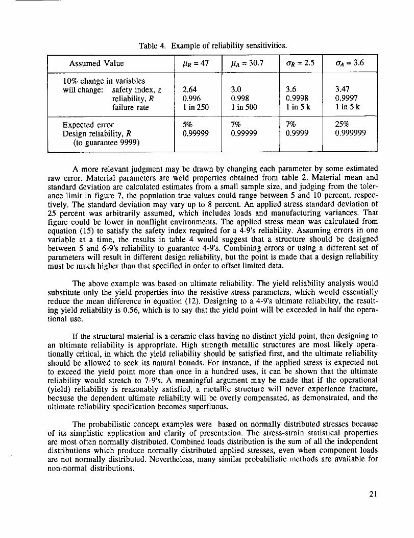
Table 4. Exampleof reliability sensitivities.

AssumedValue

10%changein variableswill change: safetyindex, z

reliability, Rfailure rate

Expected error

Design reliability, R

(to guarantee 9999)

_uR = 47

2.64

0.996

1 in 250

5%

0.99999

/.tA = 30.7

3.0

0.9981 in 500

7%

0.99999

trR = 2.5

3.6

0.9998

lin5k

7%

0.9999

trA= 3.6

3.47

0.9997

1 in5k

25%

0.999999

A more relevant judgment may be drawn by changing each parameter by some estimated

raw error. Material parameters are weld properties obtained from table 2. Material mean and

standard deviation are calculated estimates from a small sample size, and judging from the toler-

ance limit in figure 7, the population true values could range between 5 and 10 percent, respec-

tively. The standard deviation may vary up to 8 percent. An applied stress standard deviation of25 percent was arbitrarily assumed, which includes loads and manufacturing variances. That

figure could be lower in nonflight environments. The applied stress mean was calculated from

equation (15) to satisfy the safety index required for a 4-9's reliability. Assuming errors in one

variable at a time, the results in table 4 would suggest that a structure should be designed

between 5 and 6-9's reliability to guarantee 4-9's. Combining errors or using a different set of

parameters will result in different design reliability, but the point is made that a design reliability

must be much higher than that specified in order to offset limited data.

The above example was based on ultimate reliability. The yield reliability analysis would

substitute only the yield properties into the resistive stress parameters, which would essentiallyreduce the mean difference in equation (12). Designing to a 4-9's ultimate reliability, the result-

ing yield reliability is 0.56, which is to say that the yield point will be exceeded in half the opera-tional use.

If the structural material is a ceramic class having no distinct yield point, then designing to

an ultimate reliability is appropriate. High strength metallic structures are most likely opera-

tionally critical, in which the yield reliability should be satisfied first, and the ultimate reliability

should be allowed to seek its natural bounds. For instance, if the applied stress is expected not

to exceed the yield point more than once in a hundred uses, it can be shown that the ultimate

reliability would stretch to 7-9's. A meaningful argument may be made that if the operational

(yield) reliability is reasonably satisfied, a metallic structure will never experience fracture,

because the dependent ultimate reliability will be overly compensated, as demonstrated, and the

ultimate reliability specification becomes superfluous.

The probabilistic concept examples were based on normally distributed stresses because

of its simplistic application and clarity of presentation. The stress-strain statistical propertiesare most often normally distributed. Combined loads distribution is the sum of all the independent

distributions which produce normally distributed applied stresses, even when component loads

are not normally distributed. Nevertheless, many similar probabilistic methods are available fornon-normal distributions.

21

Some rather comprehensive and promising programs are evolving with stochasticmethodsthat are applicableto cumulativedamageproblems.Two currentprobabilistic programsbeing funded by NASA are the Jet PropulsionLaboratory (JPL) Probabilistic Failure Modelingand the Probabilistic StructuralAnalysis Method (PSAM). Both are particularly applicable fordetermining reliability of fatigue life, flaw propagation,and wear on propulsion systemcom-ponents.The former is a JPL project, and the latter is a team effort managedby SouthwestResearchInstitute.

IV. DETERMINISTIC SAFETY FACTOR

Aircraft of the early 30's were designed to a 6-g load factor which was known to include a

safety factor. The 17ST aluminum alloy commonly used had a 1.5 ratio of ultimate to yield

stresses. Since these aircraft performed satisfactorily without permanent deformation, the 1.5

stress ratio was arbitrarily adopted 17 as the universal safety factor by civil and military com-

munities. Commercial aircraft later imposed an additional multiplying factor of 1.15 on critical

joints and 1.33 on pressurized cabins to increase fatigue life.

Though this universally accepted safety factor has since been refined by aerospace

industries to incorporate statistically derived parameters, specified numerical safety factors are

often based on limited criteria and virtually no philosophically supporting analyses or considera-

tions of progress made in the aerostructural enterprise. This lack of an intellectual basis for the

safety factor is reflected in its unaccountable selections and legalistic compliance. Present prac-

tices are not in stride with the progress made and the immense resources spent on developing

thousands of degrees-of-freedom models to be used with safety factors, nor complex structural

tests crafted to verify them. Perhaps by revisiting the safety factor concept and by understanding

all its variables and limitations, a more systematic and coherent deterministic approach may beformulated.

A. Safety Factor Concept

Through improvements in modeling of materials and mechanics phenomena, the subjective

element of ignorance has been largely eliminated, but the variance of phenomena may be actively

reduced, though never eliminated. Therefore, the safety factor is a method to compensate forobjective variances. The conventional ultimate safety factor is a numerical value by which the

product of the safety factor, SF, and the applied stress, F A, induced by the maximum expected

load does not exceed the minimum ultimate strength, F R, of the structural material,

SFXFA = FR . (15)

It is called deterministic because each parameter is a singly determined value. The maximum and

minimum limits specified imply a statistical range of variations about their most probable value2

which are commonly expressed in a statistical format,

and

22

FA = ].tA+nACrA ,

FR = I.tR-nR err

= SF×(l.tA+naaa) ,

(16)

(17)

where /.t and _r are the mean and standard deviations referring to the applied and resistive

stresses by subscripts A and R, respectively. The number of standard deviations is noted by

multipliers nA and n R. Equations (16) and (17) represent the probable lower and upper tolerance

limits defined by equation (5) for the applied and resistive stress distributions, respectively.

Consequently, statistical data analyses and distribution variables rigorously developed for appli-

cation to the safety index of equation (12) are equally applicable to the safety factor of equations(16) and (17). Furthermore, progress made in data development and probabilistic safety methodsshould be diligently explored for application to the deterministic method.

What makes the deterministic method preferred in the drawing room is its versatile appli-

cation. Though resistive and applied stresses are statistically determined, only single valued

results need to be substituted into equation (15). Explicit values of distribution parameters

stipulated by the safety index are not necessarily required by equation (15). This convenience

allows the resistive stress to be represented by published 11 single values for an A- or B-basematerial.

Allowing the applied stress to be expressed as a single value is not only a convenience

but a frequent necessity during the design phase. If the statistical distribution is not available or

proves to be relatively insignificant, worst-on-worst applied stress cases are usually combined

and substituted into equation (15) as a single value. At the same time, it is recognized that this

versatility of accepting single value stresses may be a convenience for early design estimates,

but this may be abused by allowing incompletely developed data to creep permanently into finalsafety analyses.

The safety factor concept and properties incorporated into equations (15) through (17) are

illustrated in figure 12. The applied and resistive stress distributions are defined by probability

density functions. As in the probabilistic method, their overlapping tails suggest the probability of

failure. Since increasing the difference of the two means decreases their tail interference,/.tx-/.t A

expresses a measure of safety and becomes the focus of the structural deterministic

safety concept.

_ _ ----------J__e----- _ ----------_.

._ ..:.::::::!:

Resistive StressDistribution

Stress

Figure 12. Deterministic concept features.

The means difference is composed of three safety zones: the two tolerance limits defined

by equation (16) and the first of equations (17), and the mid-zone _. The contents of this mid

zone are fixed by the difference of equation (16) and the second of equations (17),

= SF×( l.tA+nACrA)--t.tA--na_ra

= (SF-1)X(/.tA +nAcr A) , (18)

23

and are noted to be dominatedby the conventionalsafety factor. Also note that by letting thesafetyfactor equalunity, the mid zoneis eliminated,makingF k = F a. But equating the maximum

expected applied stress with the minimum allowed ultimate resistive stress would admit the

applied stress to operate in the inelastic region of a polycrystalline material. To avoid facing a

permanently deformed structure, a minimum safety factor must be specified in this zone. Using

the yield failure as the upper limit of the limit design stress, F a = Fry, and recognizing that themaximum allowable stress is the ultimate stress, F R = Ftu, the design lower limit of the conven-

tional safety factor is established through equation (15) as

SFLL = Ftu

Fty (19)

Combining equations (15), (16), and (17) defines the difference of the two distribution

means, which is the deterministic total measure of safety,

laR-btA = l.tA (SF-1)+SF (nAfYa)+nRfYR • (20)

It turns out that each zone between the two stress distribution means contains a safety

factor to be independently specified by loads, materials, manufacturing, and stress disciplines.

These safety factors are as follows: n A is the standard deviation multiplier of the applied stress

which is specified for the desired probability that F a < Fly; n n is the standard deviation multi-

plier, or K-factor, of the resistive stress which is specified for the desired probability that F R =

<Ftu; SF is the conventional safety factor whose minimum is specified by equation (19). None of

these factors are arbitrary, and any one excessively specified may be shared with either of theother two factors.

Accordingly, the deterministic safety method is comprised of three distinct and inter-

changeable safety factors which may be jointly considered in formulating total safetyselection criteria.

The interaction of these safety factors is best assessed through two numerical examples

listed in table 5. Example No. 1 combined the universal safety factor of 1.5 with a B-basis

material and a two standard deviation applied stress. The net contribution of the conventional

safety factor to the difference of the means was 74 percent. Example No. 2 reduced the conven-tional safety factor to the equation (19) lower limit of 1.38 and increased the standard deviations

of the applied stress to three with an A-basis material. The conventional safety factor contribu-

tion decreased to 42 percent with only a 6-percent change in the difference of the mean stresses.

The coefficients of variations are abbreviated by the symbol "C" with subscripts referring to

respective distributions. These two examples clearly demonstrate the joint effects of the three

safety factors on total safety and their interchangeability.

Table 5. Safety factors interchangeability.

24

Example

NO. 1No. 2

!SF IJR

1.5 471.38 47

Assumed Variables

CR Ca nR

21.6 0.053 0.12 2.74

20.0 0.053 0.12 3.74

nA

2

3

Results

/zR -/ZA % SF

25.4 74

27.0 42

Results do not suggestwhich of the two combinationsof safety factors is preferred,butjudging from the percentchangeof safetyfactors,thereis indeeda preference.It would seemthatthe combination allowing the largest limit load stressis the more economicuser of the elasticmaterial.In comparingtheir limit load stressesderivedfrom equations(15) and (17),

11I_ nRCIOFA = _-_ (1- , (21)

example No. 2 has a slight edge, but results were too close to be conclusive. Equation (20) is the

deterministic total safety equation which, unlike the probabilistic method, satisfies the yield and

ultimate stress requirements simultaneously.

B. Correlation With Probabilistic Safety

Probabilistic and deterministic failure concepts are both governed by the amount of inter-

ference from their resistive and applied stress distributions, which are related to the difference of

their stress distribution means. Consider their approaches to defining their mean difference. Theprobabilistic method uses a specified yield or ultimate reliability value derived from a systems

analysis, from which a safety index is determined and the difference between the applied and

resistive stress means is calculated. The deterministic method determines three safety factors

independently based on their individual probability requirements and material properties. The

mean difference is then the outcome of the combined three safety factors.

Though the probabilistic and deterministic approaches to determining the stress distribu-

tion mean differences are not alike, they both control stress distribution interference which is

related to reliability. Then substituting the difference of the stress means derived in equation

(20) into the mean difference represented in equations (12), a deterministic safety index isrealized,

or

..

Z- 1 [].1 A (SF-1)+SF (nACYA)+nRCYR],

(22)

(nRCR)] •

_V/[#R CR]2' ''2 [(SF-1)+SF (naCa)+ 11R["_"-J "r_A (23)

Equation (23) not only defines the deterministic safety index, which establishes its

structural reliability through figure 11, but it further demonstrates the probabilistic nature of the

deterministic safety method.

Applying equation (23) to examples No. 1 and No. 2 in table 5, the calculated safety

indexes are 6.73 and 7.40, respectively. The corresponding reliabilities are 11-9's for example

No. 1 with the highest conventional safety factor and 13-9's for example No. 2 with the lower

safety factor. These are ultimate reliabilities in which the included conventional safety accommo-

dates the yield and ultimate requirements simultaneously, and partially explains the resulting

high 9's. Accommodating the yield requirement in the probabilistic method was also noted to

increase the ultimate reliability from 4-9's to 7-9's, but 13-9's demands examination.

25

ReducingexampleNo. 2 materialsfrom A- to B-basis and loads from 3 to 2-sigma, and

substituting into equations (20) and (23) yields a deterministic safety index of 6.24 correspond-

ing to a reliability of 10-9's. Since reducing the material and load probabilities further would be

unrealistic, the deterministic high 9's cannot be charged to its conservatism. Contrarily, the low

9's associated with the basic probabilistic method should be suspected for its compatibility withstatic stress safety.

It should be understood that reliabilities defined by equation (11) are an approximationbased on the mean and standard deviation and not on the total distribution. Reliabilities above 5

or 6-9's would seem to over extend the quality of data and the math concept. Also, a reliability of

4-9's translates into one failure in 10,000. Does specifying that reliability on a vehicle static

stress imply one failure in 10,000 missions, 10,000 vehicles, 10,000 critical stress zones, orwhat?

Nevertheless, the safety index of equation (23) provides a technique for comparing the

relative safety of one structural region to another, or a metallic structural safety with a ceramic

structure. It is useful in trade studies to assess interchange of safety factors. The fact that the

deterministic method produces high 9's clearly shows that the deterministic design produces

structures with almost a zero failure rate. Reliability appears not to be a consideration with staticloads using the deterministic method.

C. Safety Sensitivities

Safety factors selection criterion should only account for uncertainties which the designer

cannot determine in a rational manner. It should include materials performance probability andconfidence, anomalous operational loads, general manufacturing deviations, undeterminable

residual stresses, and minor handling damages. Important to the selection of safety factors which

incorporate these drivers is their effect on the total safety sensitivity. It is generally impracticalfor aerostructural guaranteed safety measures to compensate for errors in math and math model-ing.

The deterministic difference of the stress distribution means, equation (20), is a measureof total safety which includes the conventional safety factor, SF, and the standard deviation mul-

tipliers, n. Differentiating the means difference of equation (20) and dividing by it, its sensitivitiesto the three safety factors are:

_)(/ZR-/_A) SF laa (I+nACA) OSF

].lR-].lA ].lR--laa SF ' (24)

_(/-/R--/-/A) SF ].IAnAC A OnA

].IR--].IA _lR--].lA nA ' (25)

(/zR-/Za) _ laR nRCR _gnR

/-/R-/-/a /.tR-//a nR (26)

Another safety measure discovered in section IV-B was the determinist safety index

which included the same three safety factors. Differentiating the safety index of equation (23)and dividing by it for each safety factor, sensitivity expressions are:

26

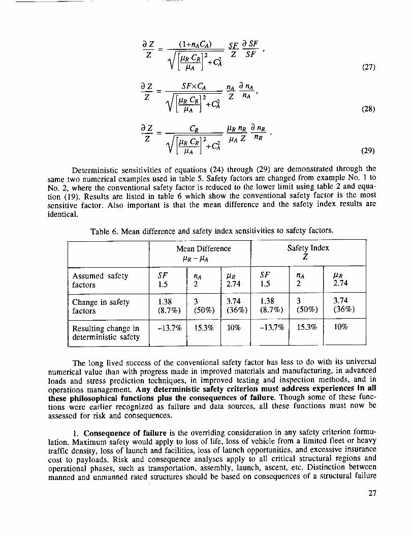
Z (I+nACA)

z _f [I_RCR] 2 _2

SF _) SF

Z SF

(27)

O___ZZ= S F x Ca n.n._&_ n A

z (28)

_)___ffZ_ CR PR n..______R_9n..____RR

Z "V'[[]'IRCR]2+C2 ]_AZ YIR[ 7-A] a (29)

Deterministic sensitivities of equations (24) through (29) are demonstrated through the

same two numerical examples used in table 5. Safety factors are changed from example No. 1 to

No. 2, where the conventional safety factor is reduced to the lower limit using table 2 and equa-

tion (19). Results are listed in table 6 which show the conventional safety factor is the most

sensitive factor. Also important is that the mean difference and the safety index results areidentical.

Table 6. Mean difference and safety index sensitivities to safety factors.

Assumed safetyfactors

Change in safetyfactors

Resulting change indeterministic safety

Mean Difference

I.tR - PA

SF

1.5

1.38

(8.7%)

-13.7%

nA

2

3

(50%)

15.3%

3.74

(36%)

10%

SF

1.5

1.38

(8.7%)

-13.7%

Safety IndexZ

nA

2

3

(50%)

15.3%

3.74

(36%)

10%

The long lived success of the conventional safety factor has less to do with its universal

numerical value than with progress made in improved materials and manufacturing, in advanced

loads and stress prediction techniques, in improved testing and inspection methods, and in

operations management. Any deterministic safety criterion must address experiences in all

these philosophical functions plus the consequences of failure. Though some of these func-tions were earlier recognized as failure and data sources, all these functions must now be

assessed for risk and consequences.

1. Consequence of failure is the overriding consideration in any safety criterion formu-

lation. Maximum safety would apply to loss of life, loss of vehicle from a limited fleet or heavy

traffic density, loss of launch and facilities, loss of launch opportunities, and excessive insurance

cost to payloads. Risk and consequence analyses apply to all critical structural regions and

operational phases, such as transportation, assembly, launch, ascent, etc. Distinction betweenmanned and unmanned rated structures should be based on consequences of a structural failure

27

in a crew environment.Consequencesmay rangefrom crewcomfort to safereturn. Cost of pro-jected payloads and launch vehicles is narrowing the consequencesbetween manned andunmannedstructures.Weight may beconsideredasa consequenceof cost.

2. Material improvements have had the most significant effects on safety. Experience

data based on material performance in related applications should have maximum influence on

safety. New materials and new applications pose the highest risk. Development of higher specific

strength materials reduces the performance sensitivity as well as the associated reduction in

strength to yield ratios. Improved quality controls establish reliable mean values and reduce data

scatter, which combine to improve the safety index of equation (23). Ductile materials in redun-dant structures sustain loads with increasing displacement better than brittle materials.

Increasing sample sizes improves the mean and variance data base and increases confidence.

3. Manufacturing variances in machining, processing, and reproducibility may be

improved to within specified economic allowance through advanced technology and quality control

enforcement. It is important to know the type and control of variances allowed for the particular

class of structure and the consequence of allowed variances. Also consider that tight controls

promised are not always deliverable.

4. Models of induced flight loads are the most unpredictable of all models. Worse yet,

they can be verified only through a limited sample of flight tests, which suggests their safety

leans heavily on consequence considerations. Deterministic loads may require minimum safetymeasures; however, high energy pressure vessels must also consider serious consequences.

Structural modeling inaccuracies are not considered in guaranteed safety factors if the structure is

test verified. Otherwise, modeling uncertainties may be covered by safety factors, but is not

accounted in the guaranteed factor. In general, prediction techniques are constantly changing andimproving, and it is necessary to verify their accuracies before incorporating safety measures.

5. Testing is indispensable to verify guaranteed safety factors on critical structures.

Improved testing techniques, instrumentation, and data recording methods have increased the

thoroughness of structural verification and test data reliability. Testing diminishes uncertainties,

exposes sneak phenomena, and serves as a feedback for fine tuning modeling accuracies, all of

which are rationale for assessing risk.

6. Inspection improved methods and techniques not only promote their application to

screen structures to increase reliably, but also allow significant reductions in safety measures.

Inspected manufactured welds allow lower safety factors than uninspected welded articles.

Scheduled inspection and maintenance reduce risk.

7. Operations management and mission rules have the capacity and authority to insure

that the guaranteed safety is never exceeded during operations. This is true for whatever the

design specified safety may be or to whatever it may degenerate. Management may choose to

methodically increase the operational experience base, but never quite operates in worst-on-

worst environments. A vehicle may be designed for all weather conditions, but it might be more

prudent to postpone a flight that is not window critical. Measuring prelaunch environments and

referring them to vehicle load indicators reduces structural risk.

Returning to the new role of the conventional safety factor, its lower limit was estab-

lished, and its sole purpose in the deterministic safety index was seen to satisfy the yield and

ultimate conditions simultaneously. The conventional universally adopted numerical value of 1.5

28

was also basedon the ratio of the ultimate to yield stresses,which wisely capitalized on the"wasteland" region of stressbeyond the elastic limit. Since operationally applied stressesarerestricted to the linear elastic region, the excessstrain energy between yield and ultimatestresseswas concededto anomalousevents without penalty to material performance for theoperational range.

The universal numerical factor wasbasedon a basicmaterialuseda half-centuryearlier.In light of currently improved propertiesof common metalsand developmentof new ones, itshouldbe fitting to comparehow well this universalfactor hasenduredover a few selectmetallicmaterialsused in contemporaryaerostructures.

Figures 13and 14graphicallycompareconventionalsafetyfactor characteristicsof ferrousand nonferrousmaterials. The first bar (darkestbar) in each group representsthe lower limitsafety factor defined by equation(19) andis estimatedfrom the left scale.Propertiesusedwerepublished11A-basis in tension and at room temperature. A general observation about the ratiosis that materials with highest heat treatment have the lowest ratio.

Dividing equation (19) by an arbitrary conventional safety factor and calculating the per-

cent change,

FSF=[S Ftu 1]x 100,V x Fry (30)

introduces a significant design consideration. The second, third, and fourth bars of each material

in figures 13 and 14 are based on equation (30) and represent the percent elastic stress per-formance denied the structure when applying arbitrary conventional safety factors of 1.5, 1.4, and

1.25, respectively. The percent loss of material performance is read from the right scale in the

figures.

\SFLL 1-F1.4

1.4 -"

_ 1.0

"_ 0.8

0.6

0.4

0.2

Low Alloy Intermed HiAllo'D6AC Cr-Mo-V 17-4 P

1.5 SF

1.25 SF

° "1/2 Hdeg 3/4 H Full Hd

D301 Stainless

26

24 mcff

20

16 8_

8 _o_0

4 _

Figure 13. Safety factor characteristics of ferrous materials.

It may be noted from equation (30) and charts that selecting a safety factor in excess ofthe lower limit defined by equation (19) could squander any economy in structures that might

have been gained from materials research and development. A safety factor of 1.5 on titaniumwastes a quarter of its elastic carrying capability. On the other hand, specifying a 1.4 safety fac-

tor on one-half hard stainless steel, having a 1.5 ultimate to yield stress ratio, would allow the

applied stress to operate into the inelastic region.

29

_-SFL rF1.4F.

_d 1.61.4 26 _

1.2 .... 24 u_1.o 20_0.8 16 o_£

._1

0.6 12 _.

E 0.40.2

A12124 AI 2219 AI 2219 I AI 7075 Ti-6A1 InconelAI 6061 -T87 ForgingJ -41 718

Figure 14. Safety factor characteristics of nonferrous materials.

Another example of judgment based on engineering analysis is to assess the structural

economy which may be equated to weight. Since conventional safety factors primarily affect

structural thicknesses, the weight change with change in safety factor may be expressed as

OW OSF

W SF (31)

where "m = 1" for plates under normal loading, and "m = 0.5" for plates in bending and buckling.Equation (31) should have no voting power over safety in selecting the numerical factor, but it

should be a serious upper limit consideration in trade studies. Proponents to delete structural

verification tests of common aerospace shell structures by increasing the lower limit safety factor

from 1.4 to 2.0 must face a 42 percent weight increase. This weight penalty is conveyed through

manufacturing, spares, handling, propulsion system, propellant, and payload and associatedcosts.

D. Safety Factors Selection Criterion

Having discovered that the deterministic safety method incorporates three safety factors,

their individual purposes, risks, consequences, sensitivities, and weight penalties must be

pooled into safety factors selection criteria. Though independently selected, safety factors in the

three safety zones interact and combine to provide one safety index which conceptually may bedeveloped into a criterion for each category of consequence. In the meantime, a selection criteria

base follows with the prospect that each safety factor will be concisely specified by respectivedisciplines.

1. Resistive Stress Zone: The material ultimate stress safety factor "nR" is identically

the K-factor of figure 5 which specifies the number of standard deviations of the resistive stress

distribution. It is selected on the basis of probability and confidence level required and, thus, is

specified as an A or B-basis material property. The A-basis is usually specified for primary

structures having high risk and severe consequences. It is specified for brittle and uncommon

materials, new applications, large coefficients of variations, limited process controls and inspec-

tions. The B-basis is specified for secondary and redundant structures where performance domi-nates and consequences will not stall, suspend or abort missions.

30

There is little experiencewith ceramicmaterialsasprimary structures.Carbon fibers andglassplatesare includedamongthesematerials.If their applicationsareweight andhazardcriti-cal, comprehensivetest programsin related environmentsmust be initiated using very large

sample sizes, satisfying probability and confidence requirements

2. Mid Zone: The mid zone safety factor is the conventional safety factor with the lower

limit defined by the ratio of ultimate to yield stresses. Its sole purpose is to ensure the applied

stress does not operate in the inelastic region of the structural material. The lower limit defines

the inelastic region of the material which is conceded to an extraordinary environment or missed

quality control with no penalty to the operational stress region. This is the factor that specifies

the upper tolerance limit of the applied stress. A factor less than the lower limit will cause the

operational load to deform the structure. A factor 1 percent in excess of the lower limit will reduce

structural performance an equal percent.

Ceramic materials that do not exhibit distinct inelastic regions reduce the lower limit con-

ventional safety factor to one, and provide no reserve for extraordinary events as in metallicmaterials. A factor greater than one may be desirable, but should be derived only from engineer-

ing analysis including remote operational environments, manufacturing process and inspection

controls, data sample size, and consequences. A more appropriate approach is to specify and

develop its property to a higher than A-basis. Arbitrarily assigned safety factors do not neces-

sarily diminish risks.

Increasing safety factors to compensate for modeling errors or deficiencies is not con-

sidered part of the guaranteed safety. If it is applied and the verification test proves it not to be

necessary, the excess spills into the applied stress zone which is passed on to the operational

margin.

Large safety factors specified for fittings, tubing, fasteners, etc, to survive installation,

manufacturing, and handling loads do not conform to deterministic safety methods. These safety

factors are uniquely specified by specialty industries or customized to user harsh ground opera-tions.

3. Applied Stress Zone: The safety factor in the applied stress zone is the standarddeviation multiplier "hA" of the applied stress distribution. It is a composite of multipliers applied

to dynamic and static load variances and to manufacturing deviations. If loads and manufacturing

means and tolerances are provided, distributions may be estimated from the means and from the

standard deviations assumed as one-third of the tolerances. Multipliers may be selected for each

load and manufacturing deviation component based on its significance and sensitivity to combined

applied stress and to its probability of occurrence, risk and consequences. Pressure load safety

factors are selected for the energy content and failure consequences.

Usually, safety factor selection criteria are formulated and applied by the loads community

who combine and report them as a single value 3-sigma or more limit load for an entire structure.

A more useful load description would include the mean and standard deviation such that adesigner may vary the number of standard deviations according to the consequence of failures at

different regions. The thoroughness required to reduce the number of standard deviations

depends on the performance gained.

Safety factor selection process for load, or induced stress, may sometimes involve a

formidable array of considerations with risk and consequences being foremost. Selection by the

31

numbers is not a recommended primary approach, but having selected a set of factors, a sim-

plistic decision analysis technique may provide a sobering backup. Using a matrix of three or

more criticality columns verses rows of significant consequence sources, the column population

should identify the dominant criticality. Each criticality column should be related to a specifiedstandard deviation multiplier. Consequence source weighing factors based on relative sensitivi-

ties on the applied stress may improve safety factor selections.

E. Applied Stress Split Safety Factor

An efficient stress design may be realized by separating the applied stress safety factorinto one induced by well defined loads (pressure, thrust, and inertia) and another applied to the

stress induced by less certain loads (aerodynamics, dynamics, and winds). The maximum

allowed applied stress is then the sum of the split induced stresses,

FA = FAI+FA2. (32)

The applied stress components are defined in statistical format and as rule of mixtures fractions,

FA1 = I.IAI( I +nA1CA1) = q FA , (33)

FA2 =//A2(1 +nA2CA2 ) = (l-q) FA , (34)

where subscripts 1 and 2 refer to the well defined set and less well defined set of stresses,respectively, and "q" is the well defined mixture fraction.

Distribution parameters in equations (33) and (34) are combined into equation (32)through the basic rules of statistics for combining uncorrelated variables. The mean of the overall

distribution is the algebraic sum of the means,

m

_'IA-" E ]'lAi '

i=l (35)

and the combined variance is the sum of the variances,

or

m

i=l

m

[#A,CA,]2i=x (36)

The combined applied stress concept defined by equations (32) through (36) is illustratedin figure (15).

Solving for the means from equations (33) and (34),

q FA (I-q) FA

PAl = (I+nAICA1) ' _A2 = (l+na2Ca2) '

32

Well Defined ---_ /z,tll (Applied Stresses_lh,/]_ ,ua l

;te:'sS:'L,/Less Certain I /'X" _ Combined 7

Applied Stresses Applied Stresses

_ FA2 F_ FR

Figure 15. Dual applied stress distribution concept.

Stress

and substituting into equation (35) gives the combined mean stress

q (l-q) ]l.ta = FA l+n_lCal + l+na2Ca2J " (37)

Solving for the product of the coefficient of variation and multiplier from equations (33) and

(34) gives

nalCal - q FA 1 na2CA2 = (l-q) FA -1 .PAl ' ]./a2 (38)

Treating the product squared as a variance and combining in equation (36) gives

(naCa) 2 = (na 1Ca1)2+ (nA2CA2) 2 (39)

Substituting equations (38) into (39) yields the desired combined product of the coefficient of

variation and multiplier,

naCa = Fa -1j2+[ (l-q) -1I. /za2 (40)

A similar approach may be used to combine different distributions, such as dynamic with

static loads or stresses induced by loads and manufacturing variances.

V. SAFETY VERIFICATION

Requirements for structural test articles and expectations from tests are not generally

understood. In light of the three safety factors discovered in the deterministic method of section

/V-B, test purpose and limits need to be clarified.

After all analyses have been checked for completeness and safety criterion has been

complied, there still remain four failure related prediction uncertainties that must be resolved:

accuracy of structural math model, quality control on processing and manufacturing, material

33

propertiesunder combinedload, and inducedload math models.The latter can be verified onlythrough early operational trials which are not scopedin this document.Nevertheless,its worstcasepredictedload is simulatedon a structuraltestarticle to verify the other threeuncertainties.Conventional test proceduresandgeneric resultsleadto a generalizeddiscussionon what mightbe requiredfrom a structuraltestandhow to verify deterministicsafetyprediction.

A. Test Article Requirements

A structural test article serves two major functions. It provides the user with an estimate

of the structure's safety level and failure mode, and it offers an opportunity to verify the structural

math model. A safety estimate may be achieved by simulating constraints through a test bed and

by simulating predicted worst case loading through load cells. The structure is loaded to failure,

and its safety is judged as to whether or not the failure loads exceeded predicted loads. It also

provides visual information as to the structure failure mode: fail operational, fail safe, or catas-trophic.

However, load cells alone cannot verify that the local failure was caused by the predicted

combined stress. It cannot explain the cause of failure at an unanticipated region, nor can it detect

a sneak phenomenon. Electrical strain gauges and stress coats provide that kind of data to be

used in post test analysis with the prediction model.

Strain and displacement gauges are indispensable for verifying and fine tuning the struc-

tural math model which is later used to verify the predicted operational loads. The corrected

model is particularly useful for predicting structural safety under other projected mission

environments. Another purpose for a strain gauge instrumented article is the feedback learning it

provides the modeler. Without that post test analysis, there is no creditable experience gained,which represents a meaningful loss.

A test plan must be preceded by a test prediction data base for tracking strain gauge data.

It was indicated earlier that metallic material failures most often occur near their average values.

Therefore, predictions should be extended to material average properties. It was also noted thatfailures occur in regions having abrupt local changes in geometry, metallurgy, and loads which

pose serious limitations to obtaining direct strain data. Planning must include special strain gage

applications and supporting analyses. The test structure responds to induced multiaxial combined

stresses, and failure is estimated by the minimum distortion energy theory. Biaxial strain at a

weld may be extrapolated by mounting gauges on adjacent parent surfaces as suggested by

figure 8. Transverse shears at dome-cylinder intersections, for instance, may be analyticallyderived from strain gauge data obtained along the discontinuity stress wave. Combined stresses

on shells induced by rivets and bolts in shear may be verified through strategic location of gauges

and assisted by a detailed discontinuity analysis such as might be obtained through boundaryelement methods.

Ultimately, the stress analysis is the primary authority on a structure's general safety.The structural test is required only to verify prediction models in part. The best that can be

expected from strain gauges is to verify one or two measured surface stress components at each

critical region with model predictions. Complementing electrical strain gauges with a brittle

stress coating would provide further detailed qualitative evidence on surface stress patterns forcomparison with math model predicted patterns.

34

B. Safety Data Interpretations

The most meaningful and critical phase of the deterministic safety verification test is

tracking the strain gauge data up to the structural yield point. The simulated load to the yield

point includes two safety factors--the standard deviation multipliers of applied stress and the

material yield stress K-factor. These are the only two that properly designed structures should

be expected to encounter operationally. Yield and ultimate stresses of materials with smallcoefficients of variation are expected to fail near their mean values. Therefore, gauges will track

linearly with the prediction analysis up to the article's yield point, which may be one or more

standard deviations higher than the design allowable. If the measured yield stress "FAM" on the

article exceeds the design allowable yield "FA", the difference is the operational margin, as illus-

trated in figure 16.

Applied Stress

nA_istribution _

7Predicted -_ FAYield I

Resistive StressDistribution, Ultimate _

_ Resistive Stress

_ Distributi0n, Yield ._ _l

Predicted J I I

Fracture .-_ / I I

_F_ IV

FR _

[ Fracture [

I I

1.0 [Predicted Loading Factors I 1.5

Figure 16. Structural test data interpretation.

The operational safety margin is defined by

MSoP = FAM-FAFA (41)

A simplistic conclusion to be drawn from one test is that this particular article has a veri-

fied operational margin defined by equation (41). A more important product of the test is the

comparison of load cell and strain gauge data with the structural math model. If the linear modelfaithfully tracks the test data to the yield point, then the number of applied stress standard

deviations may be estimated, and the operational margin is approximately determined. If the

model tracked the test data in rate, but not in intensity, the model may be in error by a constant.

If, on the other hand, the intensity is off in rate and intensity, the model must be examined for

global or local stiffness. Local fastener stiffness is a common cause.

Beyond the yield point to failure is the inelastic stress induced by combined, nonlinear

loads through successively deforming load paths. It exercises the cor/ventional safety factor andsome unknown number of standard deviation multipliers of the ultimate stress distribution. It

represents the resistive stress available to a one-time anomalous loads or missed manufacturing

35

deviation. It is defined as the ratio of the applied test load measured at failure with the load mea-

sured at yield. In fact, it is the same method used to determine the current safety factor, but of

less importance. Current structural testing techniques should not be expected to adequatelyverify all nonlinear predictions with all nonlinear data.

If fracture occurs in a discontinuity region, which is most likely, there are no current tech-

niques for adequately predicting inelastic stress with material properties changing simultane-

ously with geometry. To estimate the number of standard deviation multipliers experienced at

fracture, test data in discontinuity regions must be supported with an inelastic math model. With

this ultimate stress interpretation limitation in mind, the designer is ever more compelled toinsure the elastic stress verification is complete and competent, and to waive routine inelastic

testing. Test to fracture criteria should consider failure source criticality and benefit of inelastic

data verses cost of flight-like article. It is conceivable that structures with safety indexes

exceeding a specified value may be exempted from testing beyond the yield point.

VI. HUMAN FACTOR

Though structural failures are rare compared to failures in other disciplines, there are asmany structural failures today as decades ago. Recognizing progressive technological demands

and corresponding advances made, the most frequent cause of failure cited in failure investiga-

tions is incomplete analysis. It is as much a human factor as it is an administrative one. There

are many related lessons published by Drucker, Peters, Deming, etc. More relevant to mechanics

disciplines are the lessons extensively practiced and currently published by R. Ryan.18,19, 20

All such discourses should include the old truism that a design is no better than the

designer. Therefore, one starts with the best employees and even better supervisors--supervi-

sors with an infectious vision and technical credentials to inspire and perpetually advance their

staffs and technology. Switching to administrative roles must not be perceived as more presti-

gious and rewarding than improving products. World War II quartermasters wore the best boots

while the infantry got trench feet. Rewarding career opportunities should be developed forspecialists as specialists. 21

All design specialists must cultivate an instinct for spotting potential hardware problems

in manufacturing and operations. If hands-on experience is not an option, then on-site familiarity

with the hardware process is a minimum which may require priority trades for more plant travel.

There is no substitute for on-site experience. Good technologists must be nurtured. Before there

is a safe design, the concept has to grow and crackle in the mind of the designer.

VII. SUMMARY

The primary purpose of this study was to research the current arbitrary application of the

conventional safety factor and to approach the deterministic method from a probabilistic concept

leading to a more coherent philosophy and criteria for designing safer aerostructures.

It was soon realized that focus on any safety measure must be preceded by a fundamental

understanding of the source, cause, and consequences of failures and the validity and complete-

ness of data reduction, assumptions, and math models. These were discussed, and an example

36

using standardstatistical techniquesdemonstratedan incompleteanalysis as a cause of avoid-able failure. Likewise important, the statistical exercise was an educational lead into

understanding its application to probabilistic and deterministic safety methods.

A basic probabilistic safety method was used to learn the relationship of reliability and

tail interferences of the applied and the resistive stress distributions (fig. 9). It was noted that

the reliability concept produced a safety index which serves as a common multiplier of the appliedand the resistive stress distribution variances that defined the difference of the mean stresses of

the two stress distributions. Increasing the difference of the means stresses decreased tail inter-ferences which reduced the probability that a weak resistive material will encounter an excessive

applied stress.

The current deterministic concept is defined in terms of statistical tolerance limits of

applied and resistive stress distributions and a conventional safety factor. When these functions

were synthesized in figure 12, comparison with the probabilistic concept was clear. A significant

difference was that the probabilistic concept used a common safety factor, or safety index, for twozones, while the deterministic concept had three safety zones with as many different safety fac-

tors. They all served to specify the tail interferences.

It turned out that none of the deterministic safety factors are arbitrarily selected. They are

independently specified by loads, materials, manufacturing, and stress disciplines. The appliedstress safety factor is the standard deviation multiplier which specifies the desired probability

that the applied stress does not exceed the material yield point. The resistive stress safety fac-

tor is the standard deviation multiplier, or K-factor, that specifies the A- or B-basis material

property. The conventional safety factor's sole purpose is to insure that the applied stress does

not operate in the inelastic region of a metallic material, and it is defined as a ratio of ultimate to

yield stresses. Any safety factor excess may be shared with either of the other two factors.

A deterministic safety index was derived by equating the means difference of the deter-

ministic and probabilistic stress distributions. Applying the deterministic safety index to a

numerical example resulted in a deterministic reliability of over 10-9's. Reliabilities above 4-9's

should be suspected of over extending the quality of input data and reliability model. More impor-

tantly, the very large number of 9's demonstrated conclusively that the deterministic method pro-

duces nearly zero failure rates and that the method is reliability insensitive.

Nevertheless, the deterministic safety index is still a significant contribution. It con-

denses all three safety factors into a single index to support trades of safety factors. The deter-

ministic safety index may be used to calibrate or compare safety at different stressed regions or

different structures. It promises to be developed into a safety and verification criterion. It also

raises serious questions about the unequivocal three safety factors of the deterministic method

producing many more reliability 9's than the basic probabilistic method. It questions the philoso-

phy of specifying reliability levels to static stress problems. A 0.9999 reliability implies one

failure in 10,000 what?

Rationale for formulating deterministic safety criteria is presented, and deterministic ver-

ification test requirements, expectations, and data interpretation are discussed. It would seem

that a structural test article achieving the predicted yield stress plus two-thirds or more of the

material yield standard deviations should be considered a successfully verified structure. Tests

should not be routinely tested beyond that point, since the "unverified" resistive stress above the

37

yield point is a cushion to some"unpredictable"environmentalor structural phenomenawithoutpenalty to the structurallinear operationalperformance.

There were other discoveries.What wasperceived as an arbitrary method was demon-stratedto be totally investedin a statistical failure concept.What hasbeentreatedas an exclu-sive domain of the stresscommunity is a collaborationof loads,materials,stress,and manufac-turing disciplines.