STRUCTURAL AND MAGNETIC

CHARACTERIZATION OF NITROGEN ION

IMPLANTED STAINLESS STEEL AND CoCrMo

ALLOYS

A Thesis submitted to

the Graduate School of Engineering and Sciences of

İzmir Institute of Technology

in Partial Fulfilment of the Requirements for the Degree of

MASTER OF SCIENCE

in Physics

by

Mehmet FİDAN

January 2014

İZMİR

We approve the thesis of Mehmet FİDAN

Examining Committee Members:

______________________________

Prof. Dr. Orhan ÖZTÜRK

Department of Physics, Izmir Institute of Technology

______________________________

PD. Dr. Stephan MÄNDL

Plasma Physics, Leibniz-Institut für Oberflächenmodifizierung

______________________________

Assoc. Prof. Dr. Sami SÖZÜER

Department of Physics, Izmir Institute of Technology

______________________________

Prof. Dr. M. Ahmet ÖZTARHAN

Department of BioEngineering, Ege University

______________________________

Prof. Dr. Saim SELVİ

Department of Physics, Ege University

______________________________

Prof. Dr. Orhan ÖZTÜRK

Supervisor, Department of Physics,

Izmir Institute of Technology

______________________________

Prof. Dr. Nejat BULUT Head of the Department of Physics

______________________________

Prof. Dr. R. Tugrul SENGER Dean of the Graduate School of

Engineering and Sciences

03 January 2014

ACKNOWLEDGEMENTS

First of all, I would like to thank my advisor, Prof. Dr. Orhan Öztürk. His

encouragement and support made this thesis possible. I am very grateful for his

invaluable help, guidance, encouragement and his endless patience as well as his

understanding provided during this thesis. The work presented here is part of a joint

project between Department of Physics, Izmir Institute of Technology, Turkey and

Leibniz Institute of Surface Modification, Leibniz, Germany. I would like to thank Dr.

Stephan Mändle and his research group for carrying out the Plasma Immersion Ion

Implantatin (PIII) of stainless steel and CoCrMo alloys, providing nitrogen-depht and

hardness measurements. I am very thankful to TIPSAN (Izmir) for providing the

stainless steel and CoCrMo alloy materials. Special thanks go to thank the staff of

Material Research Center of Izmir Institute of Technology for their contribution. Also, I

would like to acknowledge my institution, Izmir Institute of Technology, for providing

me research facilities during my graduate study. I would like to thank Gökhan Özdemir

of MikronMak Kalıp (Manisa, Turkey) for cross-sectional sample preparation by

providing wire electrical discharge machine. My other big ‘’Thank you!’’ is to Prof. Dr.

Mustafa Güden for providing polishing system.

Finally, I can’t find better words to explain contribution of my family to my

education. Especially, I want to thank my mother for her understanding, support, and

love since elementary school.

iv

ABSTRACT

STRUCTURAL AND MAGNETIC CHARACTERIZATION OF

NITROGEN ION IMPLANTED STAINLESS STEEL AND CoCrMo

ALLOYS

Ion beam surface modification methods can be used to create hard and wear

resistant surface layers with enhanced corrosion resistance on austenitic stainless steels

(SS) and CoCr base alloys using nitrogen ions. This is mainly due to the formation of

high N content phase, γN, at relatively low substrate temperatures from about 350 to 450

ºC. This surface layer is known as an expanded austenite layer. Different N contents and

diffusion rates depending on grain orientations as well as anisotropic lattice expansion

and high residual stresses are some peculiar properties associated with the formation of

this phase. Another peculiar feature of the expanded austenite phase is related to its

magnetic character.

In this study, new data related to the magnetic nature of the expanded austenite

layers on austenitic stainless steel (304 SS) and CoCrMo alloy by nitrogen plasma

immersion ion implantation (PIII) are presented. Magnetic behaviour, nitrogen

distribution, implanted layer phases, surface topography, and surface hardness were

studied with a combination of experimental techniques involving magnetic force

microscopy, SIMS, XRD, SEM, AFM and nanoindentation method.

The experimental analyses indicate that the low temperature samples clearly

show the formation of the expanded austenite phase, while the decomposition of this

metastable phase into CrN precipitates occurs at higher temperatures. As a function of

the processing temperature, phase evolution stage for both alloys follows the same

trend: (1) initial stage of the expanded phase, γN, formation; (2) its full development,

and (3) its decomposition into CrN precipitates and the Cr-depleted matrix, fcc γ-

(Co,Mo) for CoCrMo and bcc α-(Fe,Ni) for 304 SS.

MFM imaging reveals distinct, stripe-like ferromagnetic domains for the fully

developed expanded austenite layers both on 304 SS and CoCrMo alloys. Weak domain

structures are observed for the CoCrMo samples treated at low and high processing

temperatures. The images also provide strong evidence for grain orientation dependence

of magnetic properties. The ferromagnetic state for the γN phase observed here is mainly

linked to large lattice expansions due to high N content.

v

ÖZET

AZOT İYON İMPLANTE EDİLMİŞ PASLANMAZ ÇELİK VE CoCrMo

ALAŞIMLARININ YAPISAL VE MANYETİK

KARAKTERİZASYONU

İyon demeti yüzey modifikasyon metotları, azot iyonları kullanarak ostenitik

paslanmaz çelikler ve CoCrMo baz alaşımlarının yüzeylerinde sert ve gelişmiş

korozyon direncine sahip sert yüzey tabakaları oluşturmak için kullanılabilir. Bu durum

başlıca 350 - 450 ºC gibi görece düşük altlık sıcaklıklarında yüksek N içeren γN fazı

oluşumundan ileri gelir. Bu tabaka genişlemiş ostenit tabakası olarak bilinir. Farklı N

içeriği ve difüzyon hızına bağlı olarak tane yönlenmeleri ile birlikte anizotropik kafes

genleşmesi ve yüksek artık gerilmeler bu fazın oluşumuna has özelliklerdir. Genişlemiş

ostenit fazına has bir diğer ilginç özellik de bu fazın manyetik karakteri ile ilgilidir.

Bu çalışmada, ostenitik paslanmaz çelik (304 SS) ve CoCrMo alaşımı üzerinde

azot plazma daldırma iyon implantasyonu ile oluşturulan genişlemiş ostenit

tabakalarının manyetik doğası ile ilgili yeni veriler sunulmuştur. Manyetik davranış,

azot dağılımı, implantasyon tabakası fazları, yüzey topografisi ve yüzey sertliği

manyetik kuvvet mikroskopisi, SIMS, XRD, SEM, AFM ve nanoindentasyon

metotlarını içeren deneysel teknikler bileşimiyle incelenmiştir.

Deneysel analizler, düşük sıcaklıktaki numunelerin açık bir şekilde genişlemiş

ostenit tabakası oluşumu gösterdiğine işaret ederken, yüksek sıcaklarda yarıkararlı bu

faz CrN çökeleklerine dönüşür. Faz gelişim aşamaları her iki alaşım için de işlem

sıcaklığının bir fonksiyonu olarak aynı trendi takip eder: (1) genişlemiş faz, γN,

oluşumunun başlangıç evresi; (2) tam gelişmesi ve (3) CrN çökeleklerine ve Cr fakir

matrikse bozunması (CoCrMo için fcc γ-(Co,Mo) ve 304 SS için bcc α-(Fe,Ni)).

MFM görüntülemesi, hem 304 SS hem de CoCrMo alaşım yüzeylerinde tam

oluşmuş genleşmiş ostenit tabakaları için belirgin, şerit şeklinde ferromanyetik

domainler ortaya çıkarmıştır. Düşük ve yüksek sıcaklıklarda işlem görmüş CoCrMo

numunelerinde zayıf domain yapıları gözlenmiştir. Görüntüler ayrıca manyetik

özelliklerin tane hizalanmasına olan bağımlılığı hakkında güçlü deliller sağlamaktadır.

γN fazında gözlenen ferromanyetik durum temel olarak yüksek N içeriği nedeniyle

oluşan aşırı kafes genişlemelerine bağlanmıştır.

vi

To my Family

vii

TABLE OF CONTENTS

LIST OF FIGURES ......................................................................................................... ix

LIST OF TABLES .......................................................................................................... xii

CHAPTER 1. INTRODUCTION ..................................................................................... 1

CHAPTER 2. MATERIALS AND EXPERIMENTAL METHODS ............................... 5

2.1. Austenitic Stainless Steel and CoCrMo Alloy ....................................... 5

2.2. Sample Preparation ................................................................................ 6

2.2.1. Polishing ......................................................................................... 7

2.2.2. Cross-Sectional Sample Preparation ............................................... 8

2.3. Plasma Immersion Ion Implantation (PIII) ............................................ 9

2.3.1. PIII Setup ...................................................................................... 10

2.4. Experimental Techniques ..................................................................... 11

2.4.1. X-Ray Diffraction (XRD) ............................................................. 12

2.4.1.1. Bragg-Brentano Method ..................................................... 13

2.4.1.2. Grazing Incidence X-Ray Method ...................................... 16

2.4.2. Atomic Force Microscopy (AFM) ................................................ 18

2.4.2.1. Roughness Measurements ................................................... 20

2.4.3. Magnetic Force Microscopy (MFM) ............................................ 20

2.4.4. Scanning Electron Microscopy (SEM) ......................................... 23

2.4.4.1. Energy Dispersive X-Ray (EDX) ....................................... 24

2.4.4.2. Cross-Sectional Scanning Electron Microscopy ................. 25

2.4.5. Secondary Ion Mass Spectroscopy (SIMS) .................................. 25

2.4.6. Surface Hardness Measurements .................................................. 26

CHAPTER 3. PHASE FORMATION ............................................................................ 27

3.1. Polished 304 SS and CoCrMo Substrate Alloys .................................. 27

3.2. Nitrogen Implanted 304 SS and CoCrMo Alloys ................................ 29

3.2.1. XRD Results of Nitrogen Implanted 304 SS ........................ 29

3.2.2. GIXRD Results of Nitrogen Implanted 304 SS ............................ 31

3.2.3. XRD Results of Nitrogen Implanted CoCrMo ..................... 33

viii

3.2.4. GIXRD Results of Nitrogen Implanted CoCrMo ......................... 34

3.3. Summary .............................................................................................. 36

CHAPTER 4. SURFACE TOPOGRAPHY ................................................................... 41

4.1. Substrate 304 SS and CoCrMo Alloy Surfaces ................................... 41

4.2. Nitrogen Implanted 304 SS and CoCrMo Samples ............................. 43

CHAPTER 5. MFM IMAGING ANALYSIS ................................................................ 53

5.1. Substrate 304 SS and CoCrMo Alloy Surfaces ................................... 53

5.2. Nitrogen Implanted 304 SS and CoCrMo Alloy Surfaces ................... 55

5.3. Expanded Phase (N) Magnetism ......................................................... 60

5.4. Physical Origin of Ferromagnetism in Expanded Phase ...................... 61

CHAPTER 6. COMPOSITION - DEPTH ANALYSIS ................................................. 63

6.1. Compositional Characterization ........................................................... 63

6.2. SIMS Nitrogen Concentration Depth Profiles ..................................... 66

CHAPTER 7. CROSS – SECTIONAL CHARACTERIZATION ................................. 69

CHAPTER 8. SURFACE HARDNESS ......................................................................... 74

8.1. Substrate and N Implanted 304 SS ...................................................... 74

8.2. Substrate and N Implanted CoCrMo .................................................... 76

CHAPTER 9. CONCLUSIONS ..................................................................................... 78

REFERENCES ............................................................................................................... 80

ix

LIST OF FIGURES

Figure Page

Figure 1.1. Hip implant prosthesis. ................................................................................... 1

Figure 2.1. A view of fcc γ-(Fe,Cr,Ni) and fcc γ-(Co,Cr,Mo) lattice ............................... 5

Figure 2.2. Polishing equipments ..................................................................................... 7

Figure 2.3. A cylindrical metal sample holder was used to polish bakalited cross-

sectional samples as well as disc-shaped materials ....................................... 8

Figure 2.4. A schematic diagram of PIII system ............................................................ 10

Figure 2.5. This figure illustrates Thin Film Philips X’Pert Pro MRD System which was

used for XRD experiments in this study, which was facilitated by Physics

Department in Izmir Institute of Technology .............................................. 12

Figure 2.6. Schematic diagram of XRD system in Bragg-Brentano geometry, which

belongs to thin film XRD system in Physics Department of IZTECH ........ 14

Figure 2.7. Basic geometry of Bragg-Brentano method ................................................. 15

Figure 2.8. Schematic diagram of XRD system during GIXRD measurements, which

belongs to Thin Film XRD system in Physics Department of IZTECH ...... 17

Figure 2.9. Basic geometry of GIXRD mode ................................................................. 17

Figure 2.10. A schematic of AFM tip and cantilever ..................................................... 18

Figure 2.11. Interactive forces versus distance ............................................................... 19

Figure 2.12. The first pass, for topography; the second pass, for the magnetic data ...... 21

Figure 2.13. Interaction between the magnetic tip and sample ...................................... 22

Figure 2.14. Image (left) is a topographical image of the surface of magnetic recording

tape in tapping mode. Image (right) is a MFM image of the same surface . 23

Figure 2.15. Electron beam interaction with material during SEM analysis .................. 24

Figure 2.16. The sputtering effect during SIMS ............................................................. 26

Figure 3.1. XRD patterns for the substrate 304 SS and CoCrMo alloys ........................ 28

Figure 3.2. GIXRD patterns of the substrate 304 SS at different grazing angles ........... 28

Figure 3.3. XRD data of nitrogen implanted 304 SS samples at different PIII treatment

temperatures ................................................................................................. 30

Figure 3.4. GIXRD results for N implanted 304 SS at different grazing angles from 0.5

to 10 degrees. Also, the top data in each graph belongs to XRD in θ/2θ

geometry ...................................................................................................... 32

x

Figure 3.5. XRD data for N implanted CoCrMo alloys at various PIII treatment

temperatures ................................................................................................. 33

Figure 3.6. GIXRD results for N implanted CoCrMo at different grazing angles from

0.5 to 10 degrees. Also, the top data in each graph belongs to XRD in θ/2θ

geometry ...................................................................................................... 35

Figure 3.7. Schematic drawing for the crystal structures of N implanted 304 SS at 350

°C (top) and N implanted CoCrMo at 400 °C (bottom) .............................. 36

Figure 3.8. Schematic development of phase formation of 304 SS (left) and CoCrMo

samples (right) with increasing PIII processing temperatures ..................... 37

Figure 4.1. AFM images of polished 304 SS (a) and CoCrMo (b) ................................. 41

Figure 4.2. SEM images of polished 304 SS (left) and CoCrMo (right) ........................ 42

Figure 4.3. AFM images 2-D (left) and 3-D (right) of nitrogen implanted 304 SS as a

function of PIII temperature ......................................................................... 44

Figure 4.4. SEM pictures of nitrogen implanted 304 SS at different processing

temperatures ................................................................................................. 46

Figure 4.5. AFM images 2-D (left) and 3-D (right) of nitrogen implanted CoCrMo as a

function of PIII temperature ......................................................................... 47

Figure 4.6. SEM pictures of nitrogen implanted CoCrMo at different processing

temperatures ................................................................................................. 49

Figure 4.7. RMS roughness values of the substrate samples and N implanted 304 SS and

CoCrMo samples as a function of nitrogen implantation temperature ........ 51

Figure 5.1. AFM (left) and MFM (right) images of the same regions for the polished

304 SS and CoCrMo alloy ........................................................................... 54

Figure 5.2. AFM (left) and MFM (right) images of the same regions for the N implanted

304 SS. The figure below displays the images from higher magnification for

same specimen ............................................................................................. 55

Figure 5.3. AFM (right) and MFM (right) images of the same regions for N implanted

CoCrMo at different processing temperatures ............................................. 58

Figure 6.1. The EDX measurements of the N implanted 304 SS at 350 °C (upper data)

and N implanted CoCrMo at 400 °C (lower data) ....................................... 64

Figure 6.2. SIMS nitrogen depth profiles for N implanted 304 SS samples .................. 66

Figure 6.3. SIMS nitrogen depth profiles for N implanted CoCrMo samples ................ 67

Figure 7.1. Cross-sectional SEM images of 300, 400 and 500 °C nitrogen implanted 304

SS ( refers to substrate, N refers to expanded phase) ................................ 70

xi

Figure 7.2. Cross-sectional SEM images of 300, 400 and 500 °C nitrogen implanted

CoCrMo samples (refers to substrate, N refers to expanded phase) ........ 71

Figure 7.3. Nitrogen layer thickness of N implanted samples obtained from both SEM

and SIMS results .......................................................................................... 73

Figure 8.1. Hardness of substrate and N implanted 304 SS as a fuction of indentation

depth (PIII processing temperatures from 300 to 550 °C) ........................... 75

Figure 8.2. Hardness of substrate and N implanted CoCrMo as a fuction of indentation

depth (PIII processing temperatures from 300 to 550 °C) ........................... 76

xii

LIST OF TABLES

Table Page

Table 2.1. Chemical composition in both wt.% and at.% of 304 SS and CoCrMo alloy

samples used in this study. In this table, only the main elements of the

samples are listed. The balance is either provided by Fe or Co, depending on

the alloy class. .................................................................................................. 6

Table 3.1. The 2θ centers of (111) and (200) peaks ....................................................... 39

Table 3.2. Lattice parameters, a, in Å for substrate and N implanted samples. <a>

presents average lattice constants, while Δa/a refers to the relative difference

in lattice parameters. Also, on the last column, average nitrogen contents are

given in at.%, which were obtained from EDX analysis. .............................. 39

Table 4.1. Average (Ra) and RMS roughness values of polished 304 SS and CoCrMo

alloy surfaces based on the AFM measurements. .......................................... 42

Table 4.2. Average (Ra) and root-mean-square (RMS) roughness values of polished and

N implanted 304 SS and CoCrMo surfaces based on the AFM measurements

....................................................................................................................... 51

Table 6.1. The main elemental compositions obtained by EDX for substrate 304 SS and

CoCrMo samples ........................................................................................... 63

Table 6.2. The EDX average elemental composition values of N implanted 304 SS and

CoCrMo samples as well as substrates. ......................................................... 65

Table 6.3. Thickness of nitrogen implanted layers obtained by SIMS results. .............. 68

Table 7.1. Nitrogen implanted layer thicknesses obtained from cross-sectional SEM

images. ........................................................................................................... 72

1

CHAPTER 1

INTRODUCTION

Austenitic stainless steels and CoCr alloys are widely used in medical

applications such as dental implants, bone plates, stents and prosthesis due to their high

corrosion resistance, wear resistance and biocompatibility. Figure 1.1 shows the

components of a hip prosthesis. CoCr alloys have greater wear resistance as compared

to stainless steel since CoCr alloys have the higher Cr content (∼ 30 at.%) than

austenitic stainless steels (∼ 18-20 at.%). In addition, their non-magnetic properties at

room temperature are necessary because of magnetic resonance imaging.

Figure 1.1. Hip implant prosthesis.

However, some problems are found with these materials in medical applications.

There is unavoidable corrosion and wear of them in body fluid, such as crevice

corrosion and fretting corrosion (Kamachimudali et al., 2003; Walczak et al., 1998).

These factors probably lead to an early fracture or failure of the implanted materials,

and corrosion of the implanted materials may result in release of harmful products into

the body. Another important problem is the negative effect of metal ions or fretting

debris, which can be released from the surface of the materials due to corrosion and

wear (Pulido and Parrish, 2003). When the materials are placed in body, toxic metal

2

ions such as Co, Cr and Ni may release into the body environments, which may give

rise to significant health concerns over time.

In order to improve surface properties of these materials, nitrogen ion beam

surface modification methods can be used to form protective layers on the surface of

these alloys by modifying the near surface layers of these materials (Buhagiar and

Dong, 2012; Zhang and Bell, 1985). Not only nitrogen is used in surface modification

but also carbon, boron and inert ions (Ar, He). Nitrogen has been extensively studied

with respect to others due to its abundance in nature and the results in improved

properties such as wear, corrosion resistances and also fatigue resistance.

Surface modification by inserting nitrogen ions with plasma and ion

implantation techniques offers improvements to the properties of metallic materials.

These techniques contain plasma nitriding, plasma immersion ion implantation (PIII)

and conventional beam line ion implantation. The main differences between these

techniques are the varying ion energy and the relative fraction of energetic ions,

electrons, thermal atoms and ions impinging on the surface (Roth, 2002).

In this study, the nitrogen implantation into stainless steel and CoCrMo alloys

will be carried out by plasma immersion ion implantation (PIII) method, where positive

ions are extracted from the plasma by applying negative high voltage pulses to the

substrate and simultaneously accelerated towards the whole surface. PIII is a very

appealing technique for industrial applications as it overcomes the line-of-sight

restrictions of conventional ion beam implantation and also for the possibility of

implanting complex, three-dimensional materials.

Different surface modification methods for nitrogen insertion into stainless steel

and CoCr base alloys have been described in the literature, including plasma nitriding

(Baranowska, 2004; Öztürk et al., 2011; Öztürk et al., 2009), plasma immersion ion

implantation (Lutz et al., 2011a; Manova et al., 2009) and conventional ion beam

implantation (Blawert et al., 2001; Wei et al., 1996). All these methods can be used to

create hard and wear resistant surface layers with enhanced corrosion resistance on

austenitic stainless steels (SS) and CoCr base alloys using nitrogen ions (Bazzoni et al.,

2013; Lutz et al., 2008a; Mandl and Rauschenbach, 2000; Ozturk and Williamson,

1995; Pichon et al., 2010; Williamson et al., 1994). This is mainly due to the formation

of a metastable, high N content phase, γN, at relatively low substrate temperatures from

about 350 to 450 ºC. This surface layer is known as an expanded austenite layer.

Different N contents and diffusion rates depending on grain orientation as well as

3

anisotropic lattice expansion and high residual stresses are some peculiar properties

associated with the formation of this phase (Ozturk and Williamson, 1995; Williamson

et al., 1994). Another peculiar feature of the expanded austenite phase is related to its

magnetic character: the expanded phase/layer is found to have ferromagnetic as well as

paramagnetic characteristics depending on its N contents (20-30 at.%) and associated

lattice expansions (as high as 10%) (Ozturk and Williamson, 1995).

The magnetic nature of the γN phase was first reported by Ichii et al. in 1986.

This study (K. Ichii, 1986), involving low temperature nitriding of 304 SS at 400 ºC,

found that the nitrided layer was composed of the γN phase (the term they used was S-

Phase) and was of ferromagnetic nature. A much later study (Ozturk and Williamson,

1995) involving low-energy, high-flux N implantation of 304 SS at 400 ºC revealed

more details about the magnetic nature of the γN phase. Through Mössbauer

spectroscopy and MOKE this investigation found the expanded phase to be

ferromagnetically soft in nature, and to be distributed in the highest concentration

region of the implanted layer. The γN phase transforms to the paramagnetic state deeper

into the layer as the N content and associated lattice expansion decreased. That study

(Ozturk and Williamson, 1995) suggested that the ferromagnetic γN phase is achieved

above a certain threshold of N content (above about 20 at.%). Two recent studies,

involving ion and gas-phase nitride 316 stainless steel (Basso et al., 2009; Wu et al.,

2011), however, find a lower threshold N content value, about 14 at.%, for the

ferromagnetic expanded phase. After the detailed study (Ozturk and Williamson, 1995),

a number of publications reported observations related to the magnetic character of the

γN phase formed on austenitic SSs (Fewell et al., 2000; Menéndez et al., 2008;

Menéndez et al., 2010; Öztürk et al., 2009). More recently, the ferromagnetic nature of

the γN phase in austenitic SS alloys was revealed through the observation of stripe-like

domains via magnetic force microscopy (MFM) imaging and through the observation of

hysteresis loops via magneto-optic Kerr effect (MOKE) (Menéndez et al., 2013; Öztürk

et al., 2009). In these studies, the origin of the magnetism in the γN phase is mainly

explained by large lattice expansions (due to high N contents), and should eventually be

related to the underlying origins of the magnetic effect in fcc-Fe and related alloys.

Some other researchers link the ferromagnetism of the γN phase to various defects

(stacking faults, twins, etc.) observed in the expanded phase layers (Blawert et al.,

2001).

4

While, according to literature of the last twenty years, there has been

considerable amount of research related to the expanded austenite phase in CoCr based

alloys (the expanded phase in CoCrMo alloy was first reported by Wei et al. in 2004

(Lanning and Wei, 2004)), there is only one study related to the magnetic nature of the

γN phase in this alloy system (Öztürk et al., 2011). This study involving low

temperature nitriding of CoCrMo alloy at 400 ºC provided strong evidence for the

ferromagnetic nature of the γN phase in this alloy through MFM observation of stripe

domain structures as well as the hysteresis loops obtained through MOKE analysis.

Although the expanded phase itself has now been studied in detail by various

research groups, its magnetic nature has been relegated to a minor role. Instead, the

focus rather has been on mechanical, tribological, corrosion, and biocompatibility of

expanded layers. However, there may be possible applications for magnetic γN layers on

non-magnetic substrates, underlying fcc γ phases of austenitic SS and CoCrMo alloys

have paramagnetic properties at room temperature. Two possible application areas that

may utilize the magnetism of the expanded phase may be magnetic recording (H. Sanda

et. al., 1990) and magnetic separation (very localized zone for trapping magnetic

particles) (Menéndez et al., 2008). On the other hand, the ferromagnetism of the

expanded phase is probably unwelcome for biomedical SSs and CoCr based alloys,

particularly from the view point of magnetic resonant imaging (i.e., MR compatibility).

In this research, new data related to the magnetic nature of the expanded

austenite layer/phase formed on CoCrMo and 304 SS alloys by nitrogen plasma

immersion ion implantation (PIII) is presented. The purpose of this study is to improve

our understanding of surface modification of 304 SS and CoCrMo alloy with nitrogen

plasma immersion ion implantation process. In addition to structural, topographical and

magnetic properties, nitrogen depht profiles and hardness features of the N implanted

layers at processing temperatures ranging from 300 to 550 °C for fixed one hour are

investigated. This will be accomplished by experimental characterization, using X-ray

diffraction in both /2 geometry and grazing incidence (GIXRD) mode, atomic force

microscopy (AFM), magnetic force microscopy (MFM), scanning electron microscopy

(SEM), secondary ion mass spectroscopy (SIMS), energy dispersive X-ray (EDX),

nanoindentation measurements with a Berkovic indenter.

5

CHAPTER 2

MATERIALS AND EXPERIMENTAL METHODS

2.1. Austenitic Stainless Steel and CoCrMo Alloy

Austenitic stainless steel and CoCrMo are alloys of composition Fe, Cr, Ni and

Co, Cr, Mo. Stainless steels can be divided into three different groups depending on

their crystal structure at room temperature. These are austenitic, ferritic, martensitic

stainless steel corresponding to face-centered cubic (fcc), body-centered cubic (bcc) and

body-centered tetragonal (bct) crystal lattice structure, respectively.

Austenitic stainless steel (304 SS) and cobalt-chromium-molybdenum

(CoCrMo) alloy (ISO 5832-12) are the investigated materials in this study. These

samples provided by TIPSAN are cut from cylindrical bars and used as substrates. The

specimens have disc-like geometry with a diameter of 16 mm and a thickness of 4 mm

for 304 SS; a diameter of 14 mm and a thickness of 4 mm for CoCrMo alloy. Both

materials used in this work have mainly face-centered cubic (fcc-) crystal structure and

are non-magnetic at room temperature. Figure 2.1 illustrates lattice structures of these

materials (these simulations were carried out using VESTA software program).

Figure 2.1. A view of fcc γ-(Fe,Cr,Ni) and fcc γ-(Co,Cr,Mo) lattice

6

According to literature (Öztürk et al., 2009; Öztürk et al., 2006), while the grain sizes of

304 SS are between 25 and 50 µm, the grain size of CoCrMo alloy changes from 5 to 15

µm.

The main chemical composition of the alloys used in this study is listed in Table

2.1 in weight percentage (wt.%) and atomic percentage (at.%).

Table 2.1. Chemical composition in both wt.% and at.% of 304 SS and CoCrMo alloy

samples used in this study. In this table, only the main elements of the

samples are listed. The balance is either provided by Fe or Co, depending on

the alloy class.

304 SS Cr Ni Mn Si C Fe

wt.% 18.30 8.30 1.42 0.43 0.045 Bal.

at.% 19.39 7.79 1.42 0.84 0.21 Bal.

CoCrMo Cr Mo Mn Si C Co

wt.% 27.92 5.86 0.59 0.72 0.048 Bal.

at.% 30.87 3.51 0.61 1.47 0.23 Bal.

In both alloys, chemical elements are randomly distributed on substitutional sites of the

lattice. To stabilize austenitic structure it is necessary to add about 8% nickel (Gavriljuk

and Berns, 1999). Chromium causes the formation of a very thin chromium-containing

oxide layer at the surface. This formation can help protect these alloys from corrosion.

In addition, the other elements like nickel, manganese, silicon, carbon etc. can be added

to give characteristic properties such as strength, toughness or hardenability to the alloy

(Khatak and Raj, 2002).

2.2. Sample Preparation

Sample preparation mainly involves polishing before nitrogen plasma

immersion ion implantation process. All the disc-shaped samples, obtained from

TIPSAN, were polished to mirror-like quality observed by AFM. Additionally, the

cross-sectional samples were prepared in order to observe the nitrogen implanted layer

thickness.

7

2.2.1. Polishing

Prior to nitrogen plasma immersion ion implantation process, all the specimens

were polished to mirror-like quality by using a polishing system (Buehler) at IYTE. The

polishing was performed in two steps: (i) polishing with SiC papers and (ii) polishing

with diamond suspension solutions,

i. All samples were polished with SiC grinding papers (with 320, 600, 800,

1200 grid sizes). In this case, approximately 5 N force was applied for 5

minutes. Then 2400 grinding paper was applied with the same force for 10

minutes. After each step, the samples were cleaned in distilled water.

ii. Polishing cloths and diamond suspension solutions (9 µm, 3 µm, 1 µm) were

used. For each step, a force of 5 N was applied. Firstly, 9 µm diamond

solution was used for 10 minutes. Secondly, 3 µm diamond solution was

used for 15 minutes and lastly, 1 µm diamond solution was used for 20

minutes. After each step, samples were cleaned with ethanol in ultrasonic

cleaner for 10 minutes, then cleaned in distilled water.

The main parts of the polishing equipments used in this study can be seen in Figure 2.2.

Figure 2.2. Polishing equipments

8

2.2.2. Cross-Sectional Sample Preparation

Cross-sectional sample preparation involves nitrogen implanted samples. The

idea is to measure N implanted layer thicknesses using imaging methods such as optical

microscopy, SEM and AFM. The following are the cross-sectional sample preparation

steps:

i. Firstly, nitrogen implanted samples (disc-shaped) were cut into pieces by

using wire electrical discharge machine (Mikron-Mak Kalıp, Organize

Sanayi, Manisa).

ii. Secondly, cut pieces were bakalited by Struers LaboPress-3 (4 minutes

heating at 150 °C and 4 minutes cooling).

iii. Lastly, bakalited cross-sectional samples were polished according to the

polishing procedures described above.

The polishing was one of the difficult steps of this study in terms of time.

Approximately, it was two hours for each sample. Afterwards, a cylindrical metal (with

a diameter of 7 cm, a height of 3 cm and a weight of 0.5 kg) was used to hold the

samples, as it can be seen from Figure 2.3. In this way, 3 or 5 samples depending on

sample size were attached with double-stick tape on the sample holder and polished

manually by hand. In this study, total polishing time was about 50 hours for 20 disc-

shape materials and 40 cross-sectioned samples.

Figure 2.3. A cylindrical metal sample holder was used to polish bakalited cross-

sectional samples as well as disc-shaped materials

9

2.3. Plasma Immersion Ion Implantation (PIII)

Surface modification by inserting nitrogen ions with plasma and ion

implantation techniques offers improvements to the properties of metallic materials.

These techniques include plasma nitriding, plasma immersion ion implantation (PIII)

and conventional beam line ion implantation. The main differences between these

techniques are the varying ion energy and the relative fraction of energetic ions,

electrons, thermal atoms and ions impinging on the surface (Roth, 2002).

Plasma immersion ion implantation (PIII) is a surface modification technique,

which positive ions are extracted from the plasma by applying negative high voltage

pulses to the substrate and simultaneously accelerated towards the whole surface.

Owing to the line-of-sight nature of conventional ion beam implantation, the cost of the

large ion source required for modifying large components with complicated areas is

prohibitive. Since PIII overcomes the line-of-sight restrictions of conventional ion beam

implantation, it is a versatile method for complex shaped surfaces. Thus, PIII is very

appealing for industrial applications, removes the line-of-sight and cost limitation of

conventional ion beam implantation.

Different surface modification methods by inserting nitrogen ions into stainless

steel and CoCr base alloys have been studied in the literature, including plasma

nitriding (Baranowska, 2004; Öztürk et al., 2011; Öztürk et al., 2009), plasma

immersion ion implantation (Lutz et al., 2011a; Manova et al., 2009) and conventional

ion beam implantation (Blawert et al., 2001; Wei et al., 1996). A study (Wei et al.,

1996) shows that the nitrogen concentration and depths of nitrogen-enriched layers

changed depending on the process, in which the processes applied on the samples are at

the same conditions. PIII method produces thick nitrogen-enriched layers (greater than

1 µm) at high concentrations (20-30 at.%) compared to plasma nitriding (layers less

than 1 µm thick with low N content). Here, the difference between them is the energy of

the ion beams. In PIII, the ions are highly energetic ranging between 1 keV and 100

keV, whereas the ion energies are in the range of 10-100 eV in plasma nitriding.

Sputtering is essential for nitriding/implantation of materials like stainless steel

and CoCr alloys. Sputtering removes the native oxide layer from the substrate at the

beginning of the process. In PIII, the surface is sputtered due to higher ion beam

energies compared to the plasma nitriding process. During the PIII process, pure N2

10

nitrogen gas is used. On the other hand, Ar and H2 are used before the plasma nitriding

to remove native oxide layer and sometimes N2+H2 mixtures are applied to keep the

surface layer oxide free.

2.3.1. PIII Setup

In this study, nitrogen was applied on the investigated materials by tecnique of

plasma immersion ion implantation (PIII). Schematic experimental setup of the PIII

system used in this work can be seen in Figure 2.4. The PIII experiments were carried

out using an electron cyclotron resonance (ECR) plasma source in an Ultra-High

Vacuum (UHV) chamber by Dr. Stephan Mändle’s research group in Leibniz Institute

of Surface Modification in Leipzig, Germany. The ECR plasma source operating with

frequency of 2.45 GHz at a power of 150 W generated plasma with an resulting

electron temperature and plasma density of 1.3 eV and 1.6 × 1010

cm-3

, respectively. At

a nitrogen gas flow of 150 sccm the resulting pressure during the experiments was 0.53

Pa. Negative high voltage of 10 kV with a pulse length of 15 s was applied to the

samples which were mounted on a sample holder.

Figure 2.4. A schematic diagram of PIII system

11

The nitrogen implantations were performed in the temperature range between 300 and

550 °C for fixed processing time of 1 hour. The temperature variation was achieved by

changing the pulse frequency from 0.25 kHz to 4.5 kHz. During the implantation,

external heating was switched off and the samples were heated only by the impinging

ions. The temperature was monitored using an IR pyrometer on the surface of sample

holder.

2.4. Experimental Techniques

Structural, compositional, topographical and magnetic characterization of

polished and nitrogen implanted samples were carried out by the following techniques:

θ/2θ (Bragg-Branteno) X-Ray Diffraction (XRD)

Grazing incidence X-Ray Diffraction (GIXRD)

Atomic Force Microscopy (AFM)

Magnetic Force Microscopy (MFM)

Scanning Electron Microscopy (SEM) and Energy Dispersive X-Ray (EDX)

Cross-Sectional Scanning Electron Microscopy (CS-SEM)

Secondary Ion Mass Spectroscopy (SIMS)

Phase analysis was investigated with X-ray diffraction in both θ/2θ geometry and

grazing incident (GIXRD) mode. Topography was studied by scanning electron

microscopy (SEM) and atomic force microscopy (AFM). Surface roughness was

measured by atomic force microscopy (AFM). Elemental compositions were estimated

with EDX. The N implanted layer thicknesses were measured by SEM on the polished

sample cross-sections. Nitrogen depth profiles were obtained from SIMS.

Additionally, hardness measurements on the sample surfaces were performed

with Dynamic Nanoindentation Experiment using a Berkovich tip.

12

2.4.1. X-Ray Diffraction (XRD)

X-ray diffraction can be used to identify some physical and chemical

information such as composition, crystal structure and layer thickness determination.

Basically, the information is obtained from the diffraction of x-rays by a crystalline

material, which is a process of scattering of the beam by the electrons associated with

the atoms in any crystal.

Figure 2.5 indicates basic components of XRD system in this study. The

following gives a brief explanation for these components.

Ceramic X-ray tube: the source of X-rays.

Incident beam slits: to control the axial width of the incident beam.

X-ray mirror: to maintain parallel incident beams on the sample surface.

Figure 2.5. This figure illustrates Thin Film Philips X’Pert Pro MRD System which was

used for XRD experiments in this study, which was facilitated by Physics

Department in Izmir Institute of Technology

13

Automatic beam attenuator: an absorber which is placed in the x-ray beam to

reduce its intensity by a specific factor. Automatic Beam Attenuator contains a

Ni foil that can be set to be switched in and out of the x-ray beam either at a

fixed angle or at a fixed intensity.

Goniometer: a platform that holds and moves the sample and detector.

Parallel plate collimator: consists of a set of parallel plates perpendicular to the

diffraction plane. The distance between the plates defines the acceptance angle

of the collimator. The collimator in the X-ray has equatorial acceptance of 0.27o.

Solar slit: in order to parallel the diffracted beams arriving to the detector.

Diffracted beam slits: to control the amount of the diffracted X-ray beam that is

accepted by the detector. This slit is mainly used for reflectivity measurements

to enhance the resolution at very low 2angles (less than 4o).

Proportional detector: counts the number of X-rays scattered by the sample.

In this study, two different geometries: (1) Bragg-Brentano (/2) and (2)

grazing incidence x-ray diffraction (GIXRD) mode were utilized on samples. During all

XRD measurements, X-ray tube voltage and current used were 45.0 kV and 40 mA,

respectively. XRD was performed using Cu-K radiation with the wavelength 1.5406 Å

from x-ray tube. The experimental data from XRD was collected with computer-

controlled system. The resultant XRD spectrum is in the form of the scattered X-ray

intensity (counts) versus 2 (degrees). The XRD data were evaluated to obtain accurate

peak positions and to find lattice parameter using the available software (X’Pert

HighScore and PeakFit v 4.11). Here, XRD were used to identify crystal structure,

expansion of cells, crystallite sizes.

2.4.1.1. Bragg-Brentano Method

This method is also called as /2 XRD method. The basic geometry of Bragg-

Brentano XRD was illustrated in Figure 2.6.

In this configuration (also, shown in Figure 2.7), both the sample and the

detector move step by step during the measurement. The X-ray tube is fixed in the

experiment while the sample and the detector are rotated through a goniometer. The

sample moves by the angle while the detector simultaneously moves by the angle 2.

14

During the experiment, since the incident and diffracted X-rays make the same angle to

the sample surface, structural information is obtained from only (hkl) planes parallel to

the surface, not the others. There is a disadvantage of this method that the effective

depth probed by the incident beam always changes during the scan due to the change in

the angle of the incident beam. Due to change in the incident beam angle, the effective

depth probed by the beam is increased depending on increasing incident beam angle.

This property may cause some misinterpretation if it is not taken notice on examining

for example, a material having layered-structure.

Figure 2.6. Schematic diagram of XRD system in Bragg-Brentano geometry, which

belongs to thin film XRD system in Physics Department of IZTECH

15

Figure 2.7. Basic geometry of Bragg-Brentano method

When there is constructive interference from X-rays scattered by the atomic

planes in a crystal, a diffraction peak is observed. A diffraction pattern is obtained by

measuring the intensity of scattered X-ray beam as a function of scattering angle. The

condition for constructive interference from planes with spacing d is given by Bragg’s

law. When the scattered x-ray beams satisfy the Bragg’s law in Equation 2.1, very

strong intensities known as Bragg peaks are indicated in the diffraction pattern. Also,

obtained accurate peak positions (2) from the XRD result are used in order to calculate

the lattice constant in equations below. The equation 2.2 is valid for cubic structures.

(2.1)

d =

(2.2)

In above equations,

d : distance between atomic planes (hkl)

: X-ray diffraction angles from different crystal planes

n : order of diffraction

λ : wavelength of Cu-K x-rays

h, k, l : miller indices

a : lattice constant of crystal

16

In our experiments, XRD measurements of nitrogen implanted samples as well

as substrate materials were carried out by using two x-ray diffraction systems: one is

powder diffractometer system (Philips X-Pert Pro system in Center for Materials

Research) and the other is Philips X'Pert Pro MRD System Thin Film X-Ray Diffraction

system (shown in Figure 2.5). In the first system, the XRD experiments were made with

a Bragg-Brentano (/2) geometry. The 2 range for each specimen was between 30 to

100 degrees, which gives a scan time of about 10 minutes for scan step size and time

per step used in this experiment (0.0334° and 19.685 s, respectively). The second

system was used to obtain higher quality of the XRD patterns compared to powder

diffractometer system. The XRD data was provided by scanning at long time of about 1

hour for each specimen. XRD in θ/2θ geometry were performed on nitrogen implanted

samples in the 2θ=35°-55° region. This scan range allows the observation of the region

of the (111) and (200) peaks, which are most revealing compared to the higher (hkl)

data range.

2.4.1.2. Grazing Incidence X-Ray Method

Grazing Incidence X-ray diffraction (GIXRD) was utilized to obtain further

information about near-surface crystal structures on our nitrogen implanted samples.

This method generally is used at small incident angles (e.g., 0.25°, 0.5° and 1°) on the

surface providing information from quite thin layers. GIXRD data was obtained using

the thin film x-ray diffraction system in Physics Department of IZTECH.

Figure 2.8 shows the basic geometry of the GIXRD system used in this work. In

this configuration (also, illustrated in Figure 2.9), the incident X-ray beam is fixed to a

predetermined value on the sample and only the detector rotates 2θ degrees. Being

different from the XRD in Bragg-Brentano geometry, GIXRD facilitates diffraction

from the planes which are not parallel to the sample surface.

17

Figure 2.8. Schematic diagram of XRD system during GIXRD measurements, which

belongs to Thin Film XRD system in Physics Department of IZTECH

Figure 2.9. Basic geometry of GIXRD mode

In this method, a study (Öztürk et al., 2006) in literature was estimated X-ray

penetration depth for nitrogen implanted CoCrMo alloy. There, when the incident

grazing angles are 0.5° and 1°, the penetration dephts of X-ray were found to be about

34 nm and 68 nm, respectively. Thus, only by changing the angle of incident X-ray

beam incoming on the sample, this method can provide the information layer by layer.

18

In this study, the angles () of the incident X-ray beam for examination of

polished 304 SS were fixed at 0.5°, 1°, 2°, 5°, 10°, respectively in order to obtain

further information on top surface (∼ 50-100 nm) of the sample. Afterwards, GIXRD

measurements of N implanted samples were carried out to identify phase formation with

respect the depht of N implanted layer at grazing angles of 0.5°, 1°, 2°, 3°, 4°, 5°, 10°.

The scanning range (2θ) was 35°-55°.

2.4.2. Atomic Force Microscopy (AFM)

Atomic force microscopy (AFM) was used to investigate surface roughness and

topography (i.e., grain size variations and surface defects) of the polished and nitrogen

implanted samples. As can be seen from Figure 2.10, AFM uses a sharp tip mounted on

a cantilever usually made from silicon or silicon nitride, with a very low spring constant

(∼ 0.1 – 1 N/m).

Figure 2.10. A schematic of AFM tip and cantilever

The AFM working principle is described as follows: during AFM

measurements, the probe is a tip on the end of a cantilever which bends in response to

the interactive force between the tip and the sample surface. The interactive force can be

attractive or repulsive force depending on distance between tip and sample. In the case

of interaction, this force is in ranging from nN to µN. As shown in Figure 2.11, first of

all, when the tip is far away from the sample surface, the cantilever feels no any force

from the sample surface. As the tip approaches the sample surface, the cantilever

deflects towards the sample due to attractive Van der Walls force (long range). As the

19

tip gets closer to the sample, this attraction increases and rapidly the tip touches on the

sample surface. At this time, since the repulsive coloumb forces (short range) become

dominant at very small separation (∼ 0.3 nm), instantly the tip into contact with surface

deflects up to sample. When the tip moves above the surface, the tip deflection will

reflect a change in topografy. Therefore, by measuring the cantilever deflections, the

surface topography can be obtained. In addition, this deflection occurs when dF/dz

exceeds the cantilever spring constant. According to the Hooke’s Law, deflection of the

cantilever can be written as;

(2.3)

Where the deflection of cantilever ΔZ is determined by the acting force F and spring

constant k.

Figure 2.11. Interactive forces versus distance

In this study, AFM measurements were performed in semi-contact (tapping)

mode to obtain surface morphology and roughness of the polished and nitrogen

implanted specimens by using AFM (Solver Pro 7 from NT-MDT, Russia, which was

situated Physics Department in Izmir Institute of Technology). In the tapping mode, the

cantilever is approached to the surface with low oscillation and the tip scans the surface

20

in semi contact. Namely, the tip is not mechanical contact with the surface during the

scan. During all the scans, antimony (n)-doped Si cantilever with elastic constant of 20-

80 N/m, a resonans frequency of 272-334 kHz (TESP from Veeco) was used. Surface

topography measurements on all the samples were performed at least three different

regions. Typical scan area was 30 µm x 30 µm.

2.4.2.1. Roughness Measurements

Surface roughness measurements were performed on both substrates and

nitrogen implanted samples by using AFM in tapping mode. During nitrogen PIII

process sample surfaces are subjected to sputtering which may be detrimental to the

surface quality. The aim of the measurements was to get the information about

sputtering rates and their effects on the samples of PIII at each processing temperature.

The roughness values were obtained from three different regions. And, average

roughness values were calculated for all samples. The average roughness (Ra) makes no

distinction between peaks and valley and gives the deviation in surface height. On the

other hand, root-mean-square (RMS) roughness makes standart deviation of all peaks in

a selected region. Therefore, it is expected that RMS roughness values is higher than

average roughness.

2.4.3. Magnetic Force Microscopy (MFM)

In this study, the magnetic structures of the sample surfaces were imaged with a

scanning probe microscopy (Veeco, Dimension 3100) in magnetic force mode (MFM).

In this mode, the probe is a tip coated with a ferromagnetic film (e.g., CoCr or FeNi)

gives an image showing the variation in the magnetic force between the magnetized

probe and magnetic stray field originating from the sample surface.

Magnetic force microscopy (MFM) is a powerful technique to image domain

structures of different magnetic materials. MFM is an extension of atomic force

microscopy. During the MFM measurements, topographical image and magnetic data

can be simultaneously measured using the two-pass technique, as illustrated in Figure

2.12. In the two-pass technique, the first pass in the semi-contact (tapping) mode of

operation is a standart AFM trace that maps out the surface topography along the

21

surface. Then, in the second pass (lift mode), the magnetic probe tip is lifted above the

surface of sample at a constant height in order to minimize the effect of the van der

Waals forces (ranging less than 20 nm). However, during the lift height (range 30-300

nm) the tip is more sensitive to far field magnetic force than short range van der Waals

force (Wozniak et al., 2005). In literature, a study (Neves and Andrade, 1999) is said

that magnetic interactions are between 5 and 300 nm in stainless steel. During the lift

scan, the probe is moved over the surface along the same line scanning the surface

topography. As a result of the interaction between magnetic coated tip and magnetic

sample, the infulence of magnetic forces is monitored by observing changes in resonans

frequency of the tip, the results are detected by laser/photo-detector.

Figure 2.12. The first pass, for topography; the second pass, for the magnetic data

Figure 2.13 shows the interaction between the magnetic tip and sample. During

the MFM measurements, the cantilever is deflected by the magnetic interaction force F

between the ferromagnetic tip and the stray field emanating from the sample surface.

22

F = (m.) Hs (2.4)

Where m is the magnetic moment of the tip and Hs is the magnetic stray field of

the sample. Since the magnetization of the tip is parallel to its axis, only the stray field

component perpendicular to the sample surface is detected. Thus, the for Fz acting in the

z-direction is

Fz = (m.) Hs ≈ mz

(2.5)

Figure 2.13. Interaction between the magnetic tip and sample

In our experiment, the magnetic structures of the sample surfaces were imaged

with a (Veeco, Dimension 3100) magnetic fore microscopy and a CoCr coated tip (the

MESP type supplied by Bruker company) with radius of 40 nm and resonant frequency

of 60-100 kHz was used. A lift hight of 60-300 nm was chosen for all MFM

measurements presented in this study. Before MFM analysis, magnetic tips were

remagnetised by strong stray fields above surfaces of bulk permanent magnet sample.

Additionally, MFM analysis of the magnetic recording tape was performed to ensure the

status of the magnetic tip prior to each measurement. As can be seen from Figure 2.14,

the result indicates an image, which contains information about both the topograph and

23

the magnetic properties of a surface. While the left image is the surface topography, the

right image is of magnetic stray field. The dark (light) stripes in the right image indicate

domains with a relatively upward (downward) magnetization component. These stripes

refer the individual bits recorded on the magnetic tape (Fe2O3).

Figure 2.14. Image (left) is a topographical image of the surface of magnetic recording

tape in tapping mode. Image (right) is a MFM image of the same surface

2.4.4. Scanning Electron Microscopy (SEM)

A technique to obtain elemental composition and to visualize surface structures

is scanning electron microscopy (SEM). As shown from Figure 2.15, when the primary

electron beams ranging from a few hundred eV up to 30 keV hit onto the sample

surface, electron signals are emitted. The signals most commonly used are the

secondary electrons (SE), the back-scattered electrons (BSE) and X-rays. These signals

are collected by different detectors in relation with emitted beams. When a primary

electron beam interacts with electrons of an atom in an inelastic collision, most of the

energy is transferred to the electrons of the sample. In case of that, the energy of

emitted electrons have less than about 50 eV and the emitted electrons in the surface

near regions with a few nm exit the surface. It is refered as secondary electrons (SE).

On the other hand, back-scattered electrons are obtained from the more deeper regions

(from a few nm to 100 nm) of the sample in consequence of elastically interactions

between primary electron beams and the nucleus of atom. It is known that backscattered

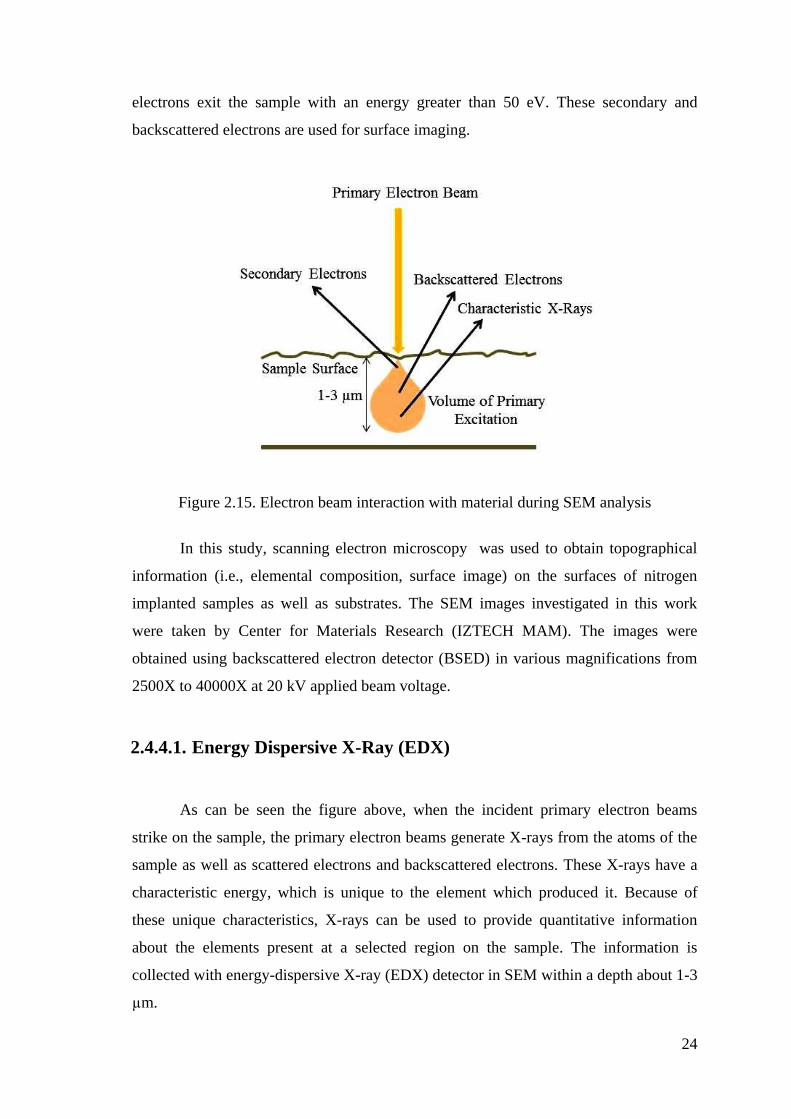
24

electrons exit the sample with an energy greater than 50 eV. These secondary and

backscattered electrons are used for surface imaging.

Figure 2.15. Electron beam interaction with material during SEM analysis

In this study, scanning electron microscopy was used to obtain topographical

information (i.e., elemental composition, surface image) on the surfaces of nitrogen

implanted samples as well as substrates. The SEM images investigated in this work

were taken by Center for Materials Research (IZTECH MAM). The images were

obtained using backscattered electron detector (BSED) in various magnifications from

2500X to 40000X at 20 kV applied beam voltage.

2.4.4.1. Energy Dispersive X-Ray (EDX)

As can be seen the figure above, when the incident primary electron beams

strike on the sample, the primary electron beams generate X-rays from the atoms of the

sample as well as scattered electrons and backscattered electrons. These X-rays have a

characteristic energy, which is unique to the element which produced it. Because of

these unique characteristics, X-rays can be used to provide quantitative information

about the elements present at a selected region on the sample. The information is

collected with energy-dispersive X-ray (EDX) detector in SEM within a depth about 1-3

µm.

25

The EDX was used to determine the elemental composition on the surfaces of

nitrogen implanted samples as well as substrates. The compositions on randomly

selected regions of specimens were taken with SEM in EDX mode. The EDX results

provided the composition ratio in units of both weight percent and atomic percent.

2.4.4.2. Cross-Sectional Scanning Electron Microscopy (CS-SEM)

In this study, cross-sectional SEM analysis was performed to measure

thichnesses of N implanted layers on the polished sample cross-sections. Before

analyzing by CS-SEM, all cross-sectional specimens were polished by polishing

procedure as mentioned earlier. During measurements, backscattered electron detector

(BSED) was used to obtain cross-sectional images. BSE images were taken at various

magnifications ranging from 10000X to 50000X by changing primary incident beam

voltages of 15 kV and 20 kV.

2.4.5. Secondary Ion Mass Spectroscopy (SIMS)

Secondary ion mass spectrometry (SIMS) is a technique that used to analyze the

elemental composition by sputtering the surface, with ppm sensitivities and lateral (x,y)

resolution between 50 nm and 2 µm (Brundle et al., 1992). As can be seen from Figure

2.16, primary ion beams (i.e., oxygen, argon) having energies between 1 and 20 keV is

focused on the surface. The energy is transferred to atoms in the surface through

collision and generates secondary particles by sputtering. As a result of that, a mixing

zone consisting of primary ions and displaced atoms from the sample occurs into

sample. The depth of the mixing zone depends on the energy, angle of incidence, mass

of the primary ions and sample. During the SIMS analysis, the primary ion beam

continuously sputters the sample and removes material from the surface. And, the

mixing zone is increased into the sample as a function of the sputtering time. The

sputtered ions (secondary ions) are extracted and accelerated towards the detector by an

electric field. By measuring their mass-to-charge ratio and their time of flight between

the sample and detector, it is possible to estimate the elemental composition of the

sample.

26

Figure 2.16. The sputtering effect during SIMS

In our work, SIMS measurements were performed using a 15 keV Ga+ beams

and a 2 keV O2+ beams for sputtering, respectively. The aim of the measurements was

to obtain the nitrogen depth distribution profiles of the nitrogen implanted samples.

2.4.6. Surface Hardness Measurements

The objective of the measurements was to investigate the hardness of nitrogen

implanted surfaces compared to substrate samples. The surface hardness values of the

samples were obtained as a function of the indentation depth.

The nanoindentation technique was developed in the mid-1970s to estimate

the hardness of small volumes of sample (Poon et al., 2008). During the measurements,

a special tip is pressed into the sample with increasing loads. The resulting hardness

value can be calculated using the contact area between tip and sample, the applied load

as well as the penetration depth.

The hardness measurements presented in this study were carried out using a

nanoindentation setup with a Berkovich tip, which has a three-sided pyramid geometry,

by Dr. Stephan Mändle’s research group in Leibniz Institute of Surface Modification in

Leipzig, Germany. The loads applied on the nitrogen implanted surfaces were 20 mN

and 50 mN, respectively. For each indentation, averaging over 10 independent

measurements technique was taken.

27

CHAPTER 3

PHASE FORMATION

In this chapter, phase analysis of nitrogen implanted samples as well as the

substrate alloys will be explained by X-ray diffraction in both θ/2θ geometry and

grazing incidence (GIXRD) mode.

3.1. Polished 304 SS and CoCrMo Substrate Alloys

Figure 3.1 presents the XRD patterns of the substrate alloys between the angles

30° and 100°. As can be seen from the substrate XRD patterns, both materials have

mainly fcc structure, which are labelled as (hkl) in Figure 3.1 and a large majority of

the fcc grains are in [111] direction.

The polished CoCrMo alloy structure consists of a mixture of predominant fcc

lattice structure [i.e., fcc -(Co,Cr,Mo)] and weak hcp crystal structure [hcp ԑ-

(Co,Cr,Mo)]. Literature indicates that the hcp ԑ phase is located, as thin bands, within

the fcc matrix. The polished 304 SS alloy has mainly fcc structure [i.e., fcc -

(Fe,Cr,Ni) phase]. The XRD data for the polished 304 SS also indicates a weak shoulder

peak just to the right of fcc (111) peak. This peak (labelled as ’) is attributed to strain-

induced martensite phase due to polishing. GIXRD analysis of this sample clearly

confirms this finding. Since ’ is to the right of the (111) peak, the GIXRD analysis

were performed in the range between the angles 35° and 55°. As can be clearly seen

from Figure 3.2, at the lowest grazing angle (°), martensite peak is much more

intense. The intensity of martensite peak decreases as a function of increasing grazing

incidence angle. As stated in the experimental method section, the penetration depth of

x-ray changes with incident angle on sample surface. At the grazing angle of 0,5° and

1°, penetration depth of x-rays (x ∼ sin/µ) is calculated as ∼41 nm, ∼82 nm,

respectively (linear mass absorption coefficient (µ) for 304 SS used in this study is 2116

cm-1

). According to the results, it can be said that martensite phase is formed on the top

surface layer (∼ 50 – 100 nm).

28

Figure 3.1. XRD patterns for the substrate 304 SS and CoCrMo alloys

Figure 3.2. GIXRD patterns of the substrate 304 SS at different grazing angles

29

3.2. Nitrogen Implanted 304 SS and CoCrMo Alloys

Here, XRD was carried out on 304 SS and CoCrMo samples that were nitrogen

implanted at temperatures ranging from 300 to 550 °C for a fixed processing time of

one hour. The XRD analyses of the nitrogen implanted samples were performed at 2θ

degrees between the angles 35° and 55°. This scan range allows the observation of the

region of the (111) and (200) peaks, which are most revealing compared to the higher

(hkl) data range.

To understand better the phase distribution with depth in the N implanted layers,

grazing incidence X-ray diffraction (GIXRD) of the N implanted samples was carried

out at the incident angles of =0.5, 1, 2, 3, 4, 5 and 10 degrees, respectively. GIXRD

analysis were also performed in the 2θ=35°-55° region. Note that the square-root of the

intensity is plotted to reveal more clearly the weaker peaks.

3.2.1. XRD Results of Nitrogen Implanted 304 SS

Figure 3.3 shows the XRD patterns of the nitrogen implanted 304 SS at various

processing temperatures. As can be seen from Figure 3.3, at lowest processing

temperature (300 °C), in addition to the substrate peaks, XRD data indicates clearly

the formation of the expanded austenite phase, labelled as N(hkl). This phase has the

same lattice structure with fcc substrate but in this phase, nitrogen atoms enter into

octahedral sites. At higher processing temperature (350 °C), as seen from the XRD data,

there is only expanded phase for this alloy and almost no substrate peaks. This indicates

that the expanded layer of this alloy is quite thick. In addition, the expanded phase

peaks corresponding to this sample are shifted to much lower angles. It means that there

is more lattice expansion and much higher nitrogen content in this sample compared to

N implanted sample at 300 °C. At the processing temperature of 400 °C, the data shows

clearly the formation of a new phase, labelled as CrN, in addition to expanded phase.

The data suggests that the expanded phase decomposes into formation of CrN. This

sample also has the expanded phase but its peaks are weaker and shifted to higher

angles compared to the samples prepared at 300 and 350 °C. At the treatment

temperature, 450 °C, the expanded phase peak intensities decreases, furthermore,

decomposition process continues not only the results into CrN but also bcc -phase [-

30

(Fe, Ni)]. At highest processing temperature (550 °C), the XRD pattern is mainly

composed of fcc CrN and bcc -(Fe, Ni) phase structures.

Figure 3.3. XRD data of nitrogen implanted 304 SS samples at different PIII treatment

temperatures

The findings here are consistent with previous studies (Collins et al., 1995; Lutz

et al., 2008a; Lutz et al., 2011b) in literature. These investigations were performed on

similar stainless steels using nitrogen PIII process.

31

3.2.2. GIXRD Results of Nitrogen Implanted 304 SS

The GIXRD results for N implanted 304 SS samples are shown as a function of

implantation temperature in Figure 3.4. In each graph of this figure, top data belongs to

the Bragg-Brentano (θ/2θ) XRD result, which was already discussed before. And the

rest are grazing incidence (GIXRD) data. The GIXRD data at the processing

temperature 300 °C show that at the lowest angle (0.5°) the N implanted layer has the

substrate peaks in addition to N peaks. The GIXRD results at higher incident angles

indicate more and more contribution coming from the substrate phase and also

increasing N phase. The GIXRD results for N implanted sample at 350 °C show that, at

all grazing angles, there are no substrate peaks. Even at highest grazing angle of 10°, the

substrate peaks does not observed, where the penetration depth of X-ray is about 4 m.

It suggests that the top layer in this sample only consists of N phase. This finding is

quite agreement with the results obtained from cross-sectional SEM and SIMS (these

results will be explained in later sections). The GIXRD data for 400 °C clearly indicates

that at the lowest grazing angle (0.5°) there are two phases: CrN and N. The intensity of

these peaks is small since the penetration depth and volume at 0.5° is less compared to

higher grazing angles. In addition, CrN and N phase intensities are increasing as a

function of grazing angle. It means that top layer is composed of CrN precipitates and

N. The GIXRD data at the processing temperature of 450 °C show that at the lowest

angles (0.5° - 1°), the top layer has only CrN and bcc -(Fe, Ni) phase. As one increases

further grazing incidence, it seems there is also contribution N phase. Further

decomposition of expanded phase is also evidenced by the grazing incidence data at 450

°C. The GIXRD results for N implanted sample at 500 °C clearly show that the top

surface layer is composed of CrN and bcc - (Fe, Ni). The data at 550 °C indicate that

at low grazing incidence angles it suggests top surface layer the phases of CrN, bcc -

(Fe, Ni) in addition to visible substrate peaks.

32

Figure 3.4. GIXRD results for N implanted 304 SS at different grazing angles from 0.5

to 10 degrees. Also, the top data in each graph belongs to XRD in θ/2θ

geometry

300 °C 350 °C

400 °C 450 °C

500 °C 550 °C

10°

5°

4°

3°

2°

1°

0.5°

33

3.2.3. XRD Results of Nitrogen Implanted CoCrMo

In Figure 3.5, the X-ray diffraction patterns of N implanted CoCrMo samples at

various processing temperatures are shown. The XRD data looks identical for

specimens processed at low temperatures (300, 350 °C). The broad peaks to the left of

the substrate ones correspond to formation of the expanded phase for this alloy system.

The N layers on CoCrMo samples at these processing temperatures are found to be

significantly thinner compared to the expanded N layers on 304 SS. At the treatment

temperature of 400 °C, the expanded layer formation is complete and a much thicker

layer is developed (no substrate peaks are visible, similar to 304 SS at 350 °C). At

processing temperatures 450 °C and above, the expanded phase is decomposing into

CrN precipitates. The precipitation of CrN depletes the expanded austenite of chromium

resulting in the formation of a mixture of fcc -CrN and the substrate phase [i.e., fcc -

Co(Mo)]. At the highest processing temperature of 550 °C, this fcc phase is quite

visible, albeit with a very low intensity and much broaden than the original substrate

peaks. The expanded layer peaks exist up to temperatures of 450 °C, suggesting that at

higher temperatures, the nitrogen containing layer is actually a mixture of CrN, and the

Cr-depleted fcc phase.

Figure 3.5. XRD data for N implanted CoCrMo alloys at various PIII treatment

temperatures

34

3.2.4. GIXRD Results of Nitrogen Implanted CoCrMo

Figure 3.6 shows the GIXRD results for N implanted CoCrMo alloy samples as

a function of implantation temperature. In this figure, the GIXRD data at the lower

processing temperature (300, 350 °C) indicate that N layer is observed at all grazing

angles (from 0.5 to 10°). However, there are no substrate peaks at = 0.5° for N

implanted specimen at 300 °C and at = 0.5°, 1° for N implanted specimen at 350 °C.

In addition, the GIXRD data at higher incident angles indicate that more contribution

from the substrate is observed. Then, the top layer (∼ 50 nm) in these samples only

consists of N phase. At the same time, the data suggests that the N implanted layer for

the sample treated 350 °C is thicker compared to the sample processed at 300 °C. The

GIXRD data for N implanted specimen at 400 °C shows that, at all grazing incident

angles, no substrate peaks are visible. And the data clearly indicates that up to grazing

incidence of 10 degrees the only phase in the layer is expanded phase, where N layer is

about 3-4 m. According to this result, the N layer thickness can be estimated with X-

ray penetration depth into this sample, which the thickness of N layer is determined

from cross-sectional SEM and SIMS results in later chapter. The GIXRD data for 450

°C clearly shows that at the lowest grazing angle of 0.5° both CrN precipitates and N

phase are visible. At this processing temperature, decomposition into CrN starts. The

GIXRD results look identical for samples processed at temperatures 500 °C and above.

For both samples, the GIXRD data clearly indicate that at low grazing incident angles

(from 0.5 to 3-4°) the peaks of N phase are not visible. It suggests that the top layer

only consists of CrN phase. As the grazing incident angles exceed up to 3-4°, it seems

that there are two phase: CrN and N phase. Additionally, the GIXRD data indicate most

intense peak of CrN in sample treated at the highest processing temperatures (500, 550

°C) compared to sample at 450 °C. This means further decomposition of expanded

phase into CrN. Then, at highest temperatures, there are only CrN precipitates in top

surface layer. Another interesting feature is that at highest processing temperatures, still

substrate peaks of the samples are visible. It suggests that N layers on CoCrMo alloys

are thinner compared to the expanded N layers on 304 SS. These results are quite

consistent with the results obtained from cross-sectional SEM and SIMS.

35

Figure 3.6. GIXRD results for N implanted CoCrMo at different grazing angles from

0.5 to 10 degrees. Also, the top data in each graph belongs to XRD in θ/2θ

geometry

300 °C 350 °C

400 °C 450 °C

500 °C 550 °C

10°

5°

4°

3°

2°

1°

0.5°

36

3.3. Summary

Figure 3.7 illustrates a schematic representation of fcc -(Fe,Cr,Ni) and -

(Co,Cr,Mo) phases resulted after the nitrogen plasma immersion ion implantation. As

shown in Figure 3.7, in these expanded phases, the nitrogen occupies octahedral sites in

the fcc -substrate lattice. These simulations were carried out using VESTA software

program. The fcc lattice of phase for N implanted 304 SS was simulated by taking

the nitrogen content 39 at.%, in which nitrogen concentration was estimated using EDX

analysis on N implanted specimen at 350 °C. For N implanted CoCrMo, nitrogen

content used in the schematic drawing was 34 at.%, which was determined by EDX

analysis on the surface of N implanted CoCrMo specimen at 400 °C.

Figure 3.7. Schematic drawing for the crystal structures of N implanted 304 SS at 350

°C (top) and N implanted CoCrMo at 400 °C (bottom)

A simple model of phase distribution in each alloy as a function of implantation

temperature is shown below. The model is based on the both XRD and GIXRD

data.

Fe Cr Ni N

Co Cr Mo N

37

Figure 3.8. Schematic development of phase formation of 304 SS (left) and CoCrMo

samples (right) with increasing PIII processing temperatures

(cont. on next page)

38

Figure 3.8. (cont.)

39

One interesting feature in Figure 3.3 and Figure 3.6 is that XRD peaks of N are

shifted to lower 2θ angles compared to the substrate peaks after nitrogen implantation

process. The main reason of these shifts is due to the expansion that nitrogen creates in

fcc lattice. Table 3.1 indicates 2θ peak centers of N implanted and substrate phases after

PIII process at treatment temperatures (300, 350 °C). As can be seen in Table 3.1, the

nitrogen implanted N(200) peaks are shifted more than N(111) peaks. It means larger

lattice expansions in [200] direction than in [111] direction. It is probably due to higher

N content in [200] direction compared to [111] direction.

Table 3.1. The 2θ centers of (111) and (200) peaks

PIII temperature (°C) (111)

N(111)

(200)

N(200)

304 SS

300 43.607 41.054 50.795 46.355

350 43.563 39.335 50.863 44.782

CoCrMo

300 43.737 39.953 50.949 45.815

350 43.762 40.025 50.971 45.764

Based on the XRD data of substrate and N implanted samples, 2θ values and

lattice constants were quantitatively calculated using a curve-fitting program. These

values are listed in Table 3.2.

Table 3.2. Lattice parameters, a, in Å for substrate and N implanted samples. <a>

presents average lattice constants, while Δa/a refers to the relative

difference in lattice parameters. Also, on the last column, average nitrogen

contents are given in at.%, which were obtained from EDX analysis.

304 SS

Implantation

temperature

(°C)

a(111)

(Å)

a(200)

(Å)

<a>

(Å)

<Δa>

<a>

(%)

Average

N. Content

(at.%)

Substrate 3.596 3.598 3.597 - -

300 3.808 3.917 3.863 7.5 35

350 3.967 4.048 4.008 11.4 39

400 3.812 3.814 3.814 6.2 36

40

CoCrMo

Implantation

temperature

(°C)

a(111)

(Å)

a(200)

(Å)

<a>

(Å)

< Δa>

<a>

(%)

Average

N. Content

(at.%)

Substrate 3.581 3.584 3.583 - -

300 3.908 3.961 3.935 9.8 36

350 3.902 3.965 3.934 9.8 38

400 3.858 4.007 3.933 9.9 34

450 3.837 - 3.837 7.0 36

500 3.685 3.700 3.693 3.1 33

550 3.667 3.685 3.676 2.5 31

Table 3.2 indicates the lattice constant values, a(111) and a(200) for both the

substrate and the nitrogen implanted samples. In addition, in this table, average nitrogen

concentrations can be found, which were obtained from EDX analysis.

41

CHAPTER 4

SURFACE TOPOGRAPHY

In this part, surface topography of substrate 304 SS and CoCrMo alloy samples

as well as nitrogen implanted materials is presented. The experiments were carried out

by using Atomic Force Microscopy (AFM) and Scanning Electron Microscopy (SEM).

The aim of the experiments is to investigate surface changes (i.e., roughness,

morphology) on samples as a result of nitrogen PIII process at different processing

temperatures. In addition to these, the roughness of the sample surfaces depending on

both average (Ra) and root-mean-square (RMS) were measured by AFM.

4.1. Substrate 304 SS and CoCrMo Alloy Surfaces

Before nitrogen PIII process, all 304 SS and CoCrMo samples were polished to

mirror-like quality (see materials and experimental section). After polishing, AFM and

SEM measurements were performed in order to investigate the surface topography of all

polished specimens.

Figure 4.1 shows AFM topographical images of polished 304 SS and CoCrMo

alloy with the scan area of 30 µm × 30 µm.

Figure 4.1. AFM images of polished 304 SS (a) and CoCrMo (b)

42

As can be seen from the images, the white particles on the surface of samples in both

pictures are believed to be due to polishing defect. They are likely to be diamond

particles from the polishing solution. In addition to that, the scratches on the surfaces

are seen in the figures.

The above images were analysed by AFM, and the average roughness (Ra) and

RMS (root-mean-square) roughness values for each polished sample were estimated

based on at least three different scan areas. Table 4.1 lists the roughness values obtained

from the analysis of the AFM images. As shown from Table 4.1, roughness value of

CoCrMo alloy is less than 304 SS.

Table 4.1. Average (Ra) and RMS roughness values of polished 304 SS and CoCrMo

alloy surfaces based on the AFM measurements.

Ra (nm) Rms (nm)

304 SS 2.45 4.94

CoCrMo 0.94 1.47

The SEM images of the polished 304 SS and CoCrMo alloy are shown in Figure

4.2. According to the SEM pictures, the scratches on both 304 SS and CoCrMo alloy

are clearly revealed.

Figure 4.2. SEM images of polished 304 SS (left) and CoCrMo (right)

43

4.2. Nitrogen Implanted 304 SS and CoCrMo Samples

After nitrogen PIII process, surface topographical features of N implanted 304

SS and CoCrMo samples were investigated by AFM and SEM. Figure 4.3 shows AFM

results of N implanted 304 SS samples at different processing temperatures, while

Figure 4.5 indicates AFM results of N implanted CoCrMo samples. In addition to these

AFM images, surface topographical features of N implanted 304 SS and CoCrMo

surfaces obtained via SEM are shown in Figure 4.4 and Figure 4.6, respectively.

As can be seen from the 2-D and 3-D AFM images of the N implanted 304 SS

surfaces with the scan areas of 30 µm × 30 µm in Figure 4.3, the grains are quite visible

at low processing temperatures (300, 350 °C), whereas they are not clear for 304 SS

samples processed at higher temperatures 400 °C and above. This may be due to more

sputtering effect during PIII experiment at higher processing temperatures. And also, it

may possibly be due to CrN precipitates into N implanted layer, as mentioned in both

XRD and GIXRD data. The 2-D and 3-D AFM images of N implanted CoCrMo

samples with the scan areas of 30 µm × 30 µm are illustrated in Figure 4.5. There, at all

PIII processing temperatures, the grain shape and sizes of N implanted CoCrMo

samples are quite visible.

The SEM images of the N implanted 304 SS samples at different processing

temperatures are given in Figure 4.4. As shown in the figure, the grains of N implanted

samples processed at lowest temperatures (300, 350 °C) are quite visible. However, as

the treatment temperature increases, this visibility becomes weak. Surface topographical

features of N implanted CoCrMo surfaces obtained via SEM are shown in Figure 4.6.

One can clearly see the grains which become quite visible as the processing temperature

increases compared to 304 SS.

Both AFM and SEM images correlate quite well for each sample category. In

addition, the images give information about grain size of the sample. As can be seen

from the all AFM and SEM images, the nitrogen implantation process does not change

grain sizes of investigated samples in this study.

44

Figure 4.3. AFM images 2-D (left) and 3-D (right) of nitrogen implanted 304 SS as a

function of PIII temperature

(cont. on next page)

10 µm

10 µm

10 µm

300 °C 2-D 3-D

350 °C 2-D 3-D

400 °C 2-D 3-D

45

Figure 4.3. (cont.)

10 µm

10 µm

10 µm

450 °C 2-D 3-D

500 °C 2-D 3-D

550 °C 2-D 3-D

46

Figure 4.4.SEM pictures of nitrogen implanted 304 SS at different processing

temperatures

300 °C 350 °C

500 °C 550 °C

400 °C 450 °C

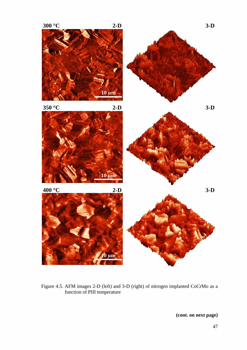
47

Figure 4.5. AFM images 2-D (left) and 3-D (right) of nitrogen implanted CoCrMo as a

function of PIII temperature

(cont. on next page)

10 µm

10 µm

10 µm

300 °C 2-D 3-D

350 °C 2-D 3-D

400 °C 2-D 3-D

48

Figure 4.5. (cont.)

10 µm

10 µm

10 µm

450 °C 2-D 3-D

500 °C 2-D 3-D

550 °C 2-D 3-D

49

Figure 4.6. SEM pictures of nitrogen implanted CoCrMo at different processing

temperatures

300 °C 350 °C

500 °C 550 °C

400 °C 450 °C

50

One feature obtained from both AFM and SEM images is that the N implanted

samples at all treatment temperatures do not have a homogenous grain structure on the

surface, grain size and shape change through the surface. It may be due to that the

different grains may have different roughness values depending on different grains have

different lattice expansions (implying different N contents). In addition, as can be

clearly seen from the SEM pictures, the grain size of N implanted 304 SS samples is

larger than N implanted CoCrMo samples. A study (Öztürk et al., 2006) in literature

shows that the grain sizes for CoCrMo samples change from 5 µm to 15 µm. Another

study (Öztürk et al., 2009) indicates that the grain size of austenitic stainless steel (SS)

changes range between 25 µm and 50µm.

As can be seen from the figures obtained from both AFM and SEM, there is a

clear evidence that the nitrogen implanted surfaces are rougher than the polished

substrate surfaces. During the nitrogen PIII process, AFM and SEM results show that

significantly a sputtering effect is revealed. And, also this sputtering is much more

intense as the processing temperature increases. As discussed in the experimental

section, in order to increase the processing temperature, pulse frequency is increased

and this results in higher nitrogen ion beam. The sputtering increase may be due to

higher nitrogen coming on the samples. The surface roughness increases as a function

of processing temperature. Although there is a significant sputtering, the images clearly

show that the grain size remains the same.

Table 4.2 lists the average and RMS roughness values of N implanted surfaces

as well as polished surfaces. Also, these RMS roughness values of the all samples are

shown in Figure 4.7. As can be seen from the table and figure, roughness values of N

implanted samples increase as a function of PIII processing temperature. While the

roughness of the 304 SS is approximately 31 nm, the average roughness of CoCrMo

surface is about 61 nm for the samples processed at 500 °C. Here, the higher increase in

roughness values is revealed for N implanted 304 SS at 350 °C, whereas it becomes for

N implanted CoCrMo at processing temperature of 400 °C. It may be due to that, as

mentioned in XRD results, N formation in both 304 SS and CoCrMo samples fully was

revealed these temperatures. And, larger lattice expansion rates for differently oriented

grains are revealed into samples processed at these temperatures.

51

Table 4.2. Average (Ra) and root-mean-square (RMS) roughness values of polished and

N implanted 304 SS and CoCrMo surfaces based on the AFM

measurements

304 SS CoCrMo

T (°C) Ra (nm) Rms (nm) Ra (nm) Rms (nm)

substrate 2.4 4.9 0.9 1.5

300 17.0 23.6 17.1 22.8

350 48.5 63.2 27.7 36.0

400 40.8 51.9 59.5 75.1

450 42.1 53.8 60.3 77.6

500

550

31.2

46.7

41.3

59.2

60.9

60.5

79.0

78.3

Figure 4.7. RMS roughness values of the substrate samples and N implanted 304 SS and

CoCrMo samples as a function of nitrogen implantation temperature

As shown the AFM images, some grains in a specimen appear to be higher than

others. White grains refer to have been higher compared to dark grains. It can be said

that the different grains may have different roughness values depending on that different

grains have different lattice expansions. According to the XRD results, the lattice

expansion of (200) oriented grains is higher than the lattice expansion of (111) oriented

52

grains. Therefore, the reason for unhomogenity of the surfaces may be due to different

nitrogen concentration of the grains as well as their different lattice expansions. Also,

the compressive stresses may contribute to the increased surface roughness of the N

implanted samples (Ozturk and Williamson, 1995).

One important feature obtained AFM and SEM images are that while the surface

changes on N implanted CoCrMo samples do not observed at all treatment temperature,

it reveals on N implanted 304 SS specimens at the processing temperature 400 °C and

above. As discussed in XRD results, for N implanted 304 SS, CrN decomposition starts

at the processing temperature 400 °C. And, CrN decomposition for N implanted

CoCrMo becomes at 450 °C. However, there is one important thing between them,

which is the intensity of CrN peaks into 304 SS is much more intense compared to

CoCrMo samples.

53

CHAPTER 5

MFM IMAGING ANALYSIS

Magnetic characterization of the polished and N implanted samples investigated

in this work was performed using magnetic force microscopy (MFM). The magnetic

structures of the sample surfaces were imaged with MFM as a result of variation in the

force between the magnetized probe and magnetic stray field originating from the

sample surface. The topographic and magnetic images of the samples were

simultaneously obtained from the same scanning regions with two-pass technique. As

mentioned before (Chapter 2, MFM), during two-pass technique in the MFM

measurements, both topography and magnetic image are obtained simultaneously; the

second pass is executed with displacement from the first pass level, which can be

changed from sample to sample. In our experiments, it was tried different tip-sample

distances (ranging from 60 nm to 300 nm) to obtain better images. It is well-known that

while the tip-surface distance increases, the magnetic signal weakens and shows a lower

magnetic contrast. A study (Dias and Andrade, 2000) about the tip-sample distance

shows that the short-range forces do not act for distances above 20-25 nm. Magnetic

interactions are related to long-range forces, which act typically between 10 and 500 nm

depending on the sample. Magnetic interaction are commonly found between 5 and 300

nm in similar stainless steels (Neves and Andrade, 1999). In our case, at distances

around 300 nm, the magnetic interaction could still be observed for N implanted

CoCrMo alloy surfaces.

5.1. Substrate 304 SS and CoCrMo Alloy Surfaces

Figure 5.1 shows the results of MFM measurement for the polished 304 SS and

CoCrMo alloy surfaces. As can be seen from Figure 5.1, there are only scratches and

dust particles in the AFM (topographic) images of the polished samples. In the MFM

(phase) images, the magnetic structure is not observed on the surface of the polished

CoCrMo alloy, while distinct magnetic patterns are easily identified in certain region of

the MFM image taken on the surface of the polished 304 SS sample.

54

Figure 5.1. AFM (left) and MFM (right) images of the same regions for the polished

304 SS and CoCrMo alloy

The magnetic patterns on 304 SS are magnetic domains of the strain-induced martensite

phase that is formed on the top surface (∼ 50 - 100 nm) due to the polishing process,

which is confirmed by both XRD and GIXRD results. Parts of the image with no

magnetic contrast probably belong to the untransformed paramagnetic austenite. On the

other hand, it seems the polishing process does not modify the magnetic structure of the

CoCrMo alloy since no magnetic contrast in the MFM image of the polished surface of

CoCrMo alloy. Several studies (Seetharaman and Krishnan, 1981; Tavares et al., 2002)

in literature show that austenitic stainless steels may become ferromagnetic when the

martensite phase is produced by effects such as cold work deformation, stress.

55

5.2. Nitrogen Implanted 304 SS and CoCrMo Alloy Surfaces

Figure 5.2 demonstrates AFM (topographic) and MFM (phase) images taken on

the surface of N implanted 304 SS at processing temperature of 350 °C.

Figure 5.2. AFM (left) and MFM (right) images of the same regions for the N implanted

304 SS. The figure below displays the images from higher magnification for

same specimen

Stripe-like domains are quite visible in parts of the image suggestive of ferromagnetism

for the N implanted layer. There is a correlation with the XRD results which only

indicate the expanded phase layer on this sample at this temperature. On the other hand,

as can be seen from the image, there is no magnetic contrast in some grains. This may

be due to the paramagnetic N or the magnetization lies in plane (stripe domains are

typical of mostly out-of-plane magnetization).

56

In this study, MFM imaging was not possible for N implanted 304 SS samples at

other processing temperatures. We believe that this may be probably due to technical

problems. In addition to this, as shown in AFM and SEM results, some defects on the

surfaces of 304 SS samples processed at temperatures higher than 350 °C were

observed, which was due to much more sputtering during PIII process. Because of this,

MFM imaging might not able to analysed for N implanted samples at higher processing

temperatures. In literature, a study (Basso et al., 2009) of magnetic and structural

features of an ion implanted 316 SS suggest that the variations of the magnetic domain

pattern can be associated with grain boundary, crystalline defects and local deformation.

Imaging by MFM for N implanted 304 SS at higher temperatures would be

important to distinguish the ferromagnetism of the expanded phase/layer from the layer

treated at 350 °C. The XRD data for the 304 SS sample treated at 550 °C shows CrN

precipitates and the Cr-depleted matrix of bcc -(Fe, Ni) as a consequence of the

expanded phase layer decomposition. It would be interesting to investigate the surface

of this sample using MFM since bcc phase is known to be ferromagnetic.

Figure 5.3 displays a sequence of AFM/MFM images showing the surface of N

implanted CoCrMo samples with increasing processing temperatures. MFM imaging

was carried out on all N implanted CoCrMo specimens except on the sample implanted

at 300 °C. As can be seen from Figure 5.3, the ferromagnetism for the N implanted

CoCrMo surfaces is quite visible through the observation of the striped domains,

especially for the samples treated at 400 and 450 °C. The dark (light) stripe domain

patterns observed in the MFM images are up (down) modulation of out-of-plane

magnetization component. As shown from the images above, the magnetic domains in

the MFM images exhibit different patterns from one grain to another. The domain

morphology (i.e., size and shape) and the periodicity of domains even changes within a

given grain.

Different domain patterns suggest different magnetic behaviour from grain-to-

grain. For the surfaces treated at 400 and 450 °C, this is probably attributed to different

amounts of lattice expansion (due to different N contents) in the different grains as

evidenced in the XRD results. According to the XRD data, the expanded phase is the

dominant crystal structure in these surfaces, and the (200) N peak is shifted more than

the (111) N peak. The domain size/shape variations observed on the different grains

may be due to the different intrinsic magnetic properties of the expanded phase in those

57

grains. Although not carried out in this study, published papers (Menéndez et al., 2010;

Wu et al., 2011) have already established correlations between the domain structure and

crystal orientation.

Although it is not seen as distinct and striped domains on the images of the

surfaces at 400 and 450 °C, the MFM images of the sample surfaces treated at 500 and

550 °C show domain patterns/structures. The domains are much more apparent for the

sample surface treated at 550 °C compared to that at 500 °C although their XRD

patterns are nearly identical. It is also clear from the MFM images that some grains

show no magnetic contrast. This may be due to either an in-plane magnetization

component or the expanded phase with less lattice expansion (lower N content). The

latter seems more plausible since the XRD data for these samples show the expanded

phase decomposing into CrN precipitates and the Cr-depleted matrix, fcc -Co(Mo)

58

Figure 5.3. AFM (right) and MFM (right) images of the same regions for N implanted

CoCrMo at different processing temperatures

(cont. on next page)

59

Figure 5.3. (cont.)

60

5.3. Expanded Phase (N) Magnetism

The most important finding in this study is related to the magnetic nature of the

expanded austenite layer on CoCrMo alloy. The γN phase/layer on CoCrMo is found to

be ferromagnetic. The ferromagnetism is revealed through the observation of the stripe-

like domains. The result is quite new and significant, since, to the authors’ knowledge,

this is the second study to date reporting ferromagnetism for the expanded phase in this

alloy system. The original study (Öztürk et al., 2011), plasma nitriding of medical grade

CoCrMo alloy with compositions similar to the one in this research, found that the

expanded phase/layer formed at 400 ºC on this alloy has ferromagnetic properties as

evidenced through the observation of stripe domains via MFM imaging and through

hysteresis curves via MOKE. In comparison, there are quite a few studies reporting

ferromagnetism for the γN phase/layer formed on austenitic stainless steels by various

ion beam as well as gas nitriding processes (Wu et al., 2011).

In this and many other investigations, the ferromagnetism of the γN layers in

austenitic SS and CoCrMo has been made clear through the stripe domain mapping by

MFM imaging analysis (Fewell et al., 2000; Wu et al., 2011). MFM imaging is also

carried out successfully on alloyed and unalloyed ferritic and/or dual phase stainless

steels (DSS) as an alternative technique compared to destructive techniques such as

chemical etching (Batista et al., 2013; Dias and Andrade, 2000).

A careful investigation of MFM images and comparison with the XRD data

suggest a good correlation between the magnetic structure development of the surfaces

of the N implanted CoCrMo samples and the development and decomposition of the

expanded phase/layers on them. For example, the MFM image of the surface of the

CoCrMo sample implanted at 350 ºC is composed of indistinct magnetic domains with

weak magnetic contrast, while the imaging of the sample surface implanted at 400 ºC

reveals distinct, stripe domains with strong magnetic contrast. The XRD results show

that at the treatment temperature of 400 ºC, the expanded layer formation is complete

with much thicker layer in comparison to the less developed γN layer on the sample

processed at 350 ºC. This correlation also holds true for the 304 SS specimen that was N

implanted at 350 ºC (MFM image containing stripe domains and XRD data indicating

fully developed γN layer). The MFM image of the surface of the CoCrMo sample

treated at 450 ºC also shows distinct stripe domain structures. The XRD results for this

61

sample suggest CrN precipitates within the expanded phase matrix. Apparently, the

decomposed phase with precipitates in the sub-micrometer range still retains a memory

of the original magnetic structure.

The MFM images in Figures 5.1, 2 and 3 show that domain morphology (size

and shape) changes from grain-to-grain and even within a grain. This is attributed to N

content and lattice expansion variations in these grains as evidenced from the XRD

data. Also, it is likely that the γN has different intrinsic magnetic properties in differently

oriented grains. In this study, the relationship between crystal orientation and the

domain structure (for example, through both MFM and EBSD) has not been carried out,

but few such studies do exist in literature, particularly for the expanded phase layer on

SS alloy (Menéndez et al., 2008; Menéndez et al., 2010; Wu et al., 2011). There is no

such study for the expanded phase layer on CoCrMo alloy. However, an alternative

explanation involves plastic mechanical deformation due to the high stress values

present in the expanded austenite layers. As dislocation lines are appearing at the

surface within grains, exhibiting a regular, parallel spacing, an association of the

domain boundaries within grains with these dislocation lines may be possible.

5.4. Physical Origin of Ferromagnetism in Expanded Phase

The ferromagnetic state for the γN phase/layers observed in this study is mainly

linked to large lattice expansions (~ 9%) due to high N contents (~ 35 at.%) (Öztürk et

al., 2011). As an interstitial impurity, nitrogen expands the host lattices of the stainless

steel and CoCrMo alloy. At a more fundamental level, the origin of ferromagnetism in

the γN phases comes from electronic structure of Fe (for stainless steel) or Co (for

CoCrMo alloy) and more precisely from 3d orbitals. Expanding the lattice reduces the

3d-3d overlap enhancing Fe or Co magnetic moments. A plausible explanation related

to the ferromagnetism observed in the expanded austenite layer in 316 SS was recently

given by Basso et al (Basso et al., 2009). The authors claimed that the most important

effect governing the ferromagnetism is the N-Cr interaction, which removes Cr 3d

electrons from the metal alloy valence band promoting ferromagnetism. An earlier

study (Blawert et al., 2001) suggested that both the lattice expansion and the defect

density might be important for the magnetic properties of the expanded phase. This

study indicated that fine changes in the atomic distances due to the stacking faults can

62

induce paramagnetic to ferromagnetic transformation (the expanded phase normally

contains a high density of dislocations, slip lines, deformation twins, and stacking

faults).

63

CHAPTER 6

COMPOSITION - DEPTH ANALYSIS

6.1. Compositional Characterization

Elemental compositions of the nitrogen implanted 304 SS and CoCrMo samples

as well as substrate specimens were obtained by EDX. The compositions of the

substrate samples determined by the EDX analysis are listed in Table 6.1, with respect

to both at.% and wt.%. The results correlate well with the elemental compositions in

Chapter 2 that were assessed by TIPSAN.

Table 6.1. The main elemental compositions obtained by EDX for substrate 304 SS and

CoCrMo samples

Fe Cr Ni

304 SS

wt.% 73.17 18.46 8.37

at.% 72.79 19.38 7.83

Co Cr Mo

CoCrMo

wt.% 66.77 27.97 5.26

at.% 65.62 30.49 3.89

The EDX data were collected from the surfaces of substrate and N implanted

samples. Consecutive EDX measurements were taken from three different areas. One

measurement for each sample is performed on area of the selected images, as shown

Figure 6.1.

Table 6.2 lists average elemental compositions of the nitrogen implanted 304 SS

and CoCrMo samples. As can be clearly seen from Table 6.2, the average nitrogen

concentration of the N implanted layers with respect to different implantation

temperatures changes between 25 at.% and 40 at.% for 304 SS; between 31 at.% and 38

at.% for CoCrMo. The data presented in Table 6.2 correlates well with the SIMS

nitrogen concentration depth results.

64

Figure 6.1. The EDX measurements of the N implanted 304 SS at 350 °C (upper data)

and N implanted CoCrMo at 400 °C (lower data)

65

During nitrogen implantation, the nitrogen places octahedral sites in our

substrate samples’ crystal structure by decreasing the atomic weight concentration of

the base atoms (Fe, Co, Cr, Ni) in the lattice. But, as can be noticed, for the samples

processed at high temperatures 450 °C and above, the decrease in the atomic weight

concentration of Cr is less compared to the concentration decrease of Fe and Ni in 304

SS; Co and Mo in CoCrMo sample. This may be attributed to the CrN formation in N

layer agreeing with the GIXRD results at processing temperatures of 450 °C and above.

Table 6.2. The EDX average elemental composition values of N implanted 304 SS and

CoCrMo samples as well as substrates.

wt.% at.%

304 SS Fe Cr Ni N Fe Cr Ni N

Substrate 73.17 18.46 8.37 - 72.79 19.38 7.83 -

300 °C 63.28 16.67 7.00 12.57 46.02 12.89 4.79 36.09

350 °C 62.58 16.49 6.57 14.34 43.76 12.27 4.32 39.62

400 °C 62.58 17.50 7.38 12.30 45.65 13.61 5.08 35.51

450 °C 65.66 17.58 7.15 9.42 51.11 14.55 5.24 28.97

500 °C 65.34 18.08 8.18 7.75 52.88 15.58 6.72 24.79

550 °C 63.97 18.02 10.32 7.63 52.00 15.58 7.90 24.50

wt.% at.%

CoCrMo Co Cr Mo N Co Cr Mo N

Substrate 66.77 27.97 5.26 - 65.62 30.49 3.89 -

300 °C 57.84 25.04 5.17 11.95 41.58 20.26 2.26 35.88

350 °C 57.15 24.95 5.08 12.80 40.31 19.79 2.18 37.71

400 °C 58.21 25.23 5.35 11.12 42.75 20.81 2.38 34.04

450 °C 56.84 25.66 5.51 11.97 41.10 20.75 2.41 35.93

500 °C 57.91 25.80 5.55 10.73 42.90 21.47 2.50 33.15

550 °C 58.98 25.77 5.36 9.87 44.50 21.88 2.47 31.13

66

6.2. SIMS Nitrogen Concentration Depth Profiles

Nitrogen concentration profiles of the N implanted 304 SS and CoCrMo samples

were obtained by SIMS as a function of depth. Figure 6.2 and Figure 6.3 indicate SIMS

results of N implanted 304 SS and CoCrMo samples at different processing

temperatures, respectively. As can be clearly seen from the figures, a comparison of the

nitrogen depth profiles for both alloys presents a similar nitrogen distribution. The

nitrogen concentration values are quite high at the surfaces of N implanted samples

(ranging from ∼20 to ∼30 at.% for 304 SS; from ∼30 to ∼40 at.% for CoCrMo

samples). At low processing temperatures (300, 350 °C), they decrease rapidly for both

samples, while at higher processing temperatures (400, 450 °C), they decrease slowly to

a level of ∼15 at.% for 304 SS; ∼20 at.% for CoCrMo and then decrease exponentially.

The diffusion depth value reaches about 12 µm in 304 SS at 450 °C, whereas the

diffusion depth in CoCrMo alloy is about 3.2 µm for the same treatment temperature. In

this study, SIMS analyses were not performed for the nitrogen implanted 304 SS

specimens at treatment temperatures of 500 and 550 °C due to time constraints.

Figure 6.2. SIMS nitrogen depth profiles for N implanted 304 SS samples

67

Figure 6.3. SIMS nitrogen depth profiles for N implanted CoCrMo samples

A study (Lutz et al., 2008b), investigating the nitrogen diffusion into CoCr

alloys by plasma immersion ion implantation and plasma nitriding experiments at

different treatment temperatures ranging from 250 °C to 600 °C, found out that the

surface concentration of nitrogen reaches values between 30 and 35 at.%, nearly

independent of the treatment temperature.

There are few studies (Lutz et al., 2008b; Lutz and Mändl, 2009) about the

nitrogen diffusion in CoCrMo in the nitriding experiments, intended to explain the

nitrogen diffusion. The nitrogen depth profiles in austenitic stainless steel (SS) and

CoCr alloy (see Figure 6.2 and Figure 6.3) indicate plateau-type shapes slowly

decreasing from surface, followed by a rather sharp leading edge. According to the

nitrogen concentration profiles in the figures, the sharp decrease starts around 15 at.%

for 304 SS; 20 at.% for CoCrMo alloy. The nitrogen profiles obtained for CoCr alloys

in literature (Lutz et al., 2008a; Lutz et al., 2008b; Lutz and Mändl, 2009) correlate well

with data related to the nitrogen diffusion in CoCrMo samples investigated in this study.

68

Another interesting feature in Figure 6.2 and 6.3 is the average nitrogen

penetration depths of the N implanted samples. The N implanted layer thickness values

obtained by SIMS nitrogen concentration depth profiles are given in Table 6.3.

Table 6.3. Thickness of nitrogen implanted layers obtained by SIMS results.

Temperatures

T (C)

Thickness for 304 SS

(µm)

Thickness for CoCrMo

(µm)

300 1 0.4

350 4 0.8

400 9 3

450 12 3.1

500 - 2.5

550 - 2.4

As mentioned in the experimental section, during the temperature increase in the PIII

implantation process, pulse frequency is increased in order to raise the processing

temperature. This leads to higher nitrogen penetration depths due to higher pulse

frequencies which also mean higher N contents.

In a study (Manova et al., 2007), the thickness of the nitrided layer (plasma

immersion ion implantation of 304 SS at 450 °C) are measured at 5 at.% of the nitrogen

concentration in concentration-depth profile. The thickness values in Table 6.3 are

estimated by taking 5 at.% (as a reference) nitrogen concentration of the leading edge of

the nitrogen concentration depth profiles. The thickness values obtained from SIMS are

quite consistent with the cross-sectional SEM results, which it will be mentioned in

Chapter 7 (cross-section sample characterization).

Different nitrogen penetration depths for 304 SS and CoCrMo samples may be

attributed to the different Cr contents. According to EDX results, the atomic

concentration of Cr is ∼20 at.% for 304 SS, whereas the atomic concentration of Cr is

∼30 at.% for CoCrMo alloy. The Cr element might have a significant role in the

nitrogen diffusion in 304 SS and CoCrMo samples during the nitrogen implantation.

And also CoCrMo has a smaller grain size resulting in lower penetration depths in

CoCrMo grains compared to 304 SS.

69

CHAPTER 7

CROSS – SECTIONAL CHARACTERIZATION

Cross-sectional characterization of the N implanted 304 SS and CoCrMo

specimens were performed by using SEM. The cross-sectional sample preparation is

described in the materials and experimental methods (Chapter 2). The aim of the cross-

sectional characterization is mainly to estimate the N implanted layer thicknesses as

well as to investigate the phases of the N implanted layers.

Cross-sectional SEM results for the N implanted 304 SS and CoCrMo

specimens at the processing temperatures of 300, 400 and 500 °C are shown in Figure

7.1 and Figure 7.2, respectively. Note that the cross-sectional SEM images were taken

under different magnifications for more detailed view of the implanted layer. However,

here, SEM images obtained from same magnification were presented to compare

thicknesses of N implanted layer on both alloys.

Figure 7.1 shows phase formations in the N implanted layers of 304 SS at all

processing temperatures. At the lowest processing temperature of 300 °C, as seen in

Figure 7.1, there is only formation of the N phase on top surface and this expanded

layer is quite thin. At higher processing temperature, 400 °C, the N implanted layer

expands, along with the formation of a new phase, labelled as CrN. The N phase and

CrN in this N implanted layer were observed layer by layer via XRD and GIXRD. At

the processing temperature of 500 °C, the N implanted layer is composed of N, CrN,

and also bcc -(Fe,Ni) phase. These findings correlate well with surface topography

results obtained both by SEM and AFM, where CrN precipitates in N implanted 304 SS

samples processed at temperatures of 400 and 500 °C were observed.

Figure 7.2 indicates the formation of the N phases in N implanted CoCrMo

samples at the processing temperatures of 300, 400 and 500 C. At the lowest processing

temperature of 300 °C, the thickness of the N phase is very low compared to the N

implanted 304 SS at the same processing temperature. The moderately low thickness of

the implanted layer was also determined according to the XRD and GIXRD results.

At the higher processing temperature of 400 °C, the cross sectional SEM image clearly

indicates a thicker N implanted layer. The thickness of layer of the N implanted sample

70

Figure 7.1. Cross-sectional SEM images of 300, 400 and 500 °C nitrogen implanted 304

SS ( refers to substrate, N refers to expanded phase)

300 °C

400 °C

CrN

500 °C

CrN + Fe, Ni)

71

Figure 7.2. Cross-sectional SEM images of 300, 400 and 500 °C nitrogen implanted

CoCrMo samples (refers to substrate, N refers to expanded phase)

300 °C

400 °C

500 °C

72

at the processing temperature of 500 °C was approximately the same with respect to the

specimen N implanted at 400 °C.

The average thicknesses of the N implanted layers obtained from cross-sectional

SEM analyses are listed in Table 7.1. The results presented in Table 7.1 are averages of

the measurements taken from at least three different regions. According to the table, the

thicknesses of the N implanted 304 SS samples are higher compared to N implanted

CoCrMo alloys. The thickness of N implanted 304 SS at the processing temperature of

550 °C is approximately 15 µm, whereas, the thickness of N implanted CoCrMo at the

same temperature is only about 2 µm. The results suggest that nitrogen diffusion in 304

SS is much higher compared to the CoCrMo alloys. This can be explained with the

higher Cr content of CoCrMo alloy compared to 304 SS. And also, it may possibly be

due to the smaller grain sizes of the CoCrMo alloy.

Table 7.1. Nitrogen implanted layer thicknesses obtained from cross-sectional SEM

images.

Temperature

(C)

Thickness in 304 SS

(µm)

Thickness in CoCrMo

(µm)

300 1.11 0.24

350 3.24 0.48

400 10.10 2.55

450 11.50 2.70

500 14.90 2.36

550 15.13 2.06

SIMS and cross-sectional SEM data given in Table 6.3 and Table 7.1

respectively are plotted in Figure 7.3. As can be clearly seen from Figure 7.3, the

thicknesses of the N implanted samples increase as a function of nitrogen PIII

temperature due to the aforementioned chromium (Cr) content and grain size effects.

And also, in the nitrogen PIII process, pulse frequency of ions is increased in order to

raise the processing temperature. This leads to higher nitrogen penetration depths due to

higher pulse frequencies.

73

Figure 7.3. Nitrogen layer thickness of N implanted samples obtained from both SEM

and SIMS results

According to cross-sectional SEM image of the N implanted 304 SS specimen at

the processing temperature of 400 °C, N implanted layer was composed of CrN and N

phases. The distribution of CrN and N phases in the N implanted layer was revealed in

the XRD and GIXRD results that were given in Chapter 3. Depending on the XRD,

GIXRD and cross-sectional SEM results, it can be said that the upper layer may be

probably the CrN precipitates and the lower is expanded N layer. The results correlate

well with a study (Chen et al., 2008) in literature.

In the cross-sectional SEM results, -(Fe,Cr,Ni) observation is quite similar

with our cross-sectional SEM results in the literature based on nitriding of austenitic

stainless steels (Öztürk et al., 2009) and -(Co,Cr,Mo) observations based on nitriding

of CoCrMo studies (Öztürk et al., 2006).

74

CHAPTER 8

SURFACE HARDNESS

This section covers surface hardness profiles of the substrate and the nitrogen

implanted samples. The measurements were carried out by dynamic nanoindentation

experiments using a Berkovich tip. Several indentations were made applying each of the

following loads: 20 and 50 mN for each nitrogen implanted specimen.

The aim of this analysis was to investigate the hardness properties of N

implanted surfaces compared to polished samples.

8.1. Substrate and N Implanted 304 SS

The hardness of the substrate and nitrogen implanted 304 SS samples are shown

in Figure 8.1. The experiments were conducted with the substrate by applying loads of

10, 50, 100, 200, 300 mN and with the N implanted surfaces by applying loads of 20, 50

mN, respectively.

As can be clearly seen from Figure 8.1, for the polished 304 SS, at the lowest

two applied loads (10-50 mN) higher hardness values were attained. This relatively high

hardness values can be attributed to the martensite phase formation on the top surface of

polished 304 SS. This martensite phase was also confirmed on the by the XRD and

GIXRD results. On the other hand, the hardness values of the substrate decrease

gradually larger indenter loads to smaller values. This can be explained by the fact that

at higher indentation loads the penetration depth of the indenter increases resulting in

more and more contribution from the substrate phase.

The hardness values for the N implanted 304 SS samples had a nearly 5 fold

increase compared to the substrate. The increase in hardness values is attributed to only

the expanded phase layer in N implanted sample at the processing temperature of 350 C.

At higher processing temperatures the hardness increase is due to the composite matrix

of CrN and expanded N phases. Also compressive stresses effective in the N implanted

layers might contribute to the hardness. However, the hardness of 304 SS sample

processed at 300 °C was seen to be lower with respect to the N implanted samples

75

processed at other temperatures. According to the XRD, GIXRD and cross-sectional

SEM results, the thickness of the N layer processed at 300 °C is much thinner than the

other N implanted samples. This results in more contribution from the substrate phase

lowering the hardness values.

Figure 8.1. Hardness of substrate and N implanted 304 SS as a fuction of indentation

depth (PIII processing temperatures from 300 to 550 °C)

One of the important points in the graph is the average indent depths of the

indenter used in the hardness measurements. As can be seen in Figure 8.1, at the

processing temperature 350 °C and above, the indentation depths change from ∼ 0.25

m (for 20 mN load) to ∼ 0.4 m (for 50 mN load). However, at lowest treatment

temperature (300 °C), the indentation depth changes from ∼ 0.35 m to ∼ 0.65 m

corresponding to applied loads 20 and 50 mN, respectively. As mentioned in the cross-

section SEM and SIMS results, the thickness of the N implanted layer, at the treatment

temperature (300 °C) is very thin compared to samples processed at other temperatures.

According to these results, it can be explained that the indenter penetrates more in the N

implanted layer at 300 °C compared to the sample at 350 °C.

76

8.2. Substrate and N Implanted CoCrMo

Figure 8.2 indicates the hardness values of the substrate and N implanted

CoCrMo specimens. The hardness value (∼ 5 GPa) of substrate CoCrMo sample is used

as a reference, which is obtained from the literature. As can be seen from Figure 8.2, the

hardness value is the substrate CoCrMo is about 5 GPa, wheras, at the lower processing

temperatures of 300 and 350 °C the hardness values of the N implanted samples

increase up to 6-7 GPa. The small hardness increase at low temperatures are due to the

much more thinner N layer compared to the N implanted CoCrMo samples processed at

higher temperatures. As mentioned in the XRD, GIXRD and cross-sectional SEM

results, N layers on CoCrMo samples at lower processing temperatures (300 and 350

°C) are found to be significantly thinner compared to samples processed at higher

temperatures. At the higher processing temperatures of 400 °C and above, the hardness

values of the N implanted CoCrMo samples range between 12 and 15 GPa. This

increase suggests the formation of only a thicker N layer at the processing temperature

of 400 °C. At higher processing temperatures (400, 500 and 550 °C), the increased

hardness values of N implanted CoCrMo alloy may be due to CrN precipitates as well

as the formation of N phase.

Figure 8.2. Hardness of substrate and N implanted CoCrMo as a fuction of indentation

depth (PIII processing temperatures from 300 to 550 °C)

77

However, at lower processing temperatures (300, 350 °C), the hardness values of

N implanted surfaces at 20 mN are quite close to the hardness value of the substrate

material. Additionally, it could be seen that at higher indenter load, 50 mN, it

approaches the hardness value of the substrate material. It is due to more contribution of

substrate phase, as evidenced both XRD and GIXRD at low treatment temperatures of

300 and 350 °C.

These hardness results are in good correlation with the results obtained cross-

sectional SEM, XRD and SIMS analysis. According to cross-sectional SEM results,

thickness values of N phase for CoCrMo samples were measured as thinner layer (∼

0.2 m at 300 °C, ∼ 0.5 m at 350 °C) compared to other temperatures. Also, these

results correlated quite well the nitrogen depth profiles obtained by SIMS. In addition,

the both XRD and GIXRD data suggest that the N implanted CoCrMo processed at low

temperatures have thinner layer in conjunction with the peaks of substrate phase.

78

CHAPTER 9

CONCLUSIONS

In this research, new data related to magnetic nature of the expanded austenite

layer/phase formed on austenitic stainless steel (304 SS) and CoCrMo alloys by

nitrogen plasma immersion ion implantation is investigated.

The ferromagnetism of the expanded phase layers is revealed through MFM

imaging analysis of stripe-like domain structures. Combined MFM imaging analysis

and XRD data suggest a correlation exists between the magnetic structure development

and the expanded phase development and decomposition stages.

While distinct stripe domains with strong magnetic contrast are observed for the

fully developed expanded phase layers on CoCrMo (also on 304 SS), indistinct domains

with weak magnetic contrast are found for the expanded phase layer at earlier stages of

its development (i.e. processing temperatures of 300, 350 ºC) and at the stage where the

expanded phase matrix is decomposing into CrN precipitates and the Cr-depleted

matrix, fcc γ-(Co,Mo) for CoCrMo alloy and CrN precipitates plus bcc α-(Fe, Ni).

The MFM data presented suggests that the expanded phase magnetic behavior is

changing with crystallographic orientation and this is consistent with lattice expansion

and N content variations as evidenced from the XRD.

Expanded phase, γN layers are produced in the range 1 to 15 micrometre for 304

SS and range 0.2 to 3 micrometre for CoCrMo, it changes due to different PIII

processing temperatures.

The larger lattice expansions in the (200) planes are found compared to the (111)

planes for the N implanted samples.

Comparing to polished 304 SS and CoCrMo specimens, the average roughness

of the N implanted surfaces at highest treatment temperature of 550 °C increased about

15 and 60 times, respectively.

According to the SIMS profiles, the average nitrogen concentration reaches

about ranging from ∼20 to ∼30 at.% for 304 SS; from ∼30 to ∼40 at.% for CoCrMo

samples based on PIII processing temperature. The nitrogen is found to diffuse deeper

in the 304 SS compared to CoCrMo alloys.

79

Significant hardness improvements are observed for the nitrogen implanted

materials. The hardness increase is attributed to the formation of the expanded austenite

layer at lower processing temperatures. With higher treatment temperatures, nanometer

size CrN precipitates distributed within the N matrix are contributing to the enhanced

hardness.

80

REFERENCES

Baranowska, J. 2004. Characteristic of the nitride layers on the stainless steel at low

temperature. Surface and coatings Technology. 180:145-149.

Basso, R., V. Pimentel, S. Weber, G. Marcos, T. Czerwiec, I. Baumvol, and C.

Figueroa. 2009. Magnetic and structural properties of ion nitrided stainless steel.

Journal of Applied Physics. 105:124914-124914-124915.

Batista, L., U. Rabe, and S. Hirsekorn. 2013. Magnetic micro-and nanostructures of

unalloyed steels: domain wall interactions with cementite precipitates observed

by mfm. NDT & E International.

Bazzoni, A., S. Mischler, and N. Espallargas. 2013. Tribocorrosion of Pulsed Plasma-

Nitrided CoCrMo Implant Alloy. Tribology Letters. 49:157-167.

Blawert, C., H. Kalvelage, B. Mordike, G. Collins, K. Short, Y. Jirásková, and O.

Schneeweiss. 2001. Nitrogen and carbon expanded austenite produced by PI<

sup> 3</sup>. Surface and Coatings Technology. 136:181-187.

Brundle, C.R., C.A. Evans Jr, and S. Wilson. 1992. Encyclopedia of materials

characterization: surfaces, interfaces, thin films. Gulf Professional Publishing.

Buhagiar, J., and H. Dong. 2012. Corrosion properties of S-phase layers formed on

medical grade austenitic stainless steel. Journal of Materials Science: Materials

in Medicine. 23:271-281.

Chen, J., X. Li, T. Bell, and H. Dong. 2008. Improving the wear properties of Stellite 21

alloy by plasma surface alloying with carbon and nitrogen. Wear. 264:157-165.

Collins, G., R. Hutchings, K. Short, J. Tendys, X. Li, and M. Samandi. 1995. Nitriding

of austenitic stainless steel by plasma immersion ion implantation. Surface and

Coatings Technology. 74:417-424.

Dias, A., and M.S. Andrade. 2000. Atomic force and magnetic force microscopies

applied to duplex stainless steels. Applied surface science. 161:109-114.

Fewell, M., D. Mitchell, J. Priest, K. Short, and G. Collins. 2000. The nature of

expanded austenite. Surface and coatings Technology. 131:300-306.

Gavriljuk, V.G., and H. Berns. 1999. High nitrogen steels: structure, properties,

manufacture, applications. Springer.

H. Sanda, M. Takai, S. Namda, A. Chayahara, M. Satou, Appl. Phys. A. 50 (1990) 573

81

Kamachimudali, U., T. Sridhar, and B. Raj. 2003. Corrosion of bio implants. In

Sadhana (Academy Proceedings in Engineering Sciences). Vol. 28. Indian

Academy of Sciences. 601-637.

K. Ichii, K. Fujimura, T. Takase, Technol. Reports Kansai Univ., Vol. 127, 1986 p. 134.

Khatak, H.S., and B. Raj. 2002. Corrosion of austenitic stainless steels: mechanism,

mitigation and monitoring. Woodhead publishing.

Lanning, B.R., and R. Wei. 2004. High intensity plasma ion nitriding of orthopedic

materials: Part II. Microstructural analysis. Surface and Coatings Technology.

186:314-319.

Lutz, J., C. Diaz, J. Garcia, C. Blawert, and S. Mändl. 2011a. Corrosion behaviour of

medical CoCr alloy after nitrogen plasma immersion ion implantation. Surface

and Coatings Technology. 205:3043-3049.

Lutz, J., J.W. Gerlach, and S. Mändl. 2008a. PIII nitriding of fcc‐alloys containing Ni

and Cr. physica status solidi (a). 205:980-984.

Lutz, J., A. Lehmann, and S. Mändl. 2008b. Nitrogen diffusion in medical CoCrNiW

alloys after plasma immersion ion implantation. Surface and Coatings

Technology. 202:3747-3753.

Lutz, J., and S. Mändl. 2009. Effect of ion energy and chemistry on layer growth

processes during nitriding of CoCr alloys. Nuclear Instruments and Methods in

Physics Research Section B: Beam Interactions with Materials and Atoms.

267:1522-1525.

Lutz, J., D. Manova, J.W. Gerlach, M. Stormer, and S. Mandl. 2011b. Interpretation of

Glancing Angle and Bragg–Brentano XRD Measurements for CoCr Alloy and

Austenitic Stainless Steel After PIII Nitriding. Plasma Science, IEEE

Transactions on. 39:3056-3060.

Mandl, S., and B. Rauschenbach. 2000. Anisotropic strain in nitrided austenitic stainless

steel. Journal of Applied Physics. 88:3323-3329.

Manova, D., T. Höche, S. Mändl, and H. Neumann. 2009. Development of CrN

precipitates during the initial stages of PIII nitriding of stainless steel thin films.

Nuclear Instruments and Methods in Physics Research Section B: Beam

Interactions with Materials and Atoms. 267:1536-1539.

Manova, D., S. Mändl, H. Neumann, and B. Rauschenbach. 2007. Influence of grain

size on nitrogen diffusivity in austenitic stainless steel. Surface and Coatings

Technology. 201:6686-6689.

Menéndez, E., A. Martinavicius, M. Liedke, G. Abrasonis, J. Fassbender, J.

Sommerlatte, K. Nielsch, S. Suriñach, M. Baró, and J. Nogués. 2008. Patterning

of magnetic structures on austenitic stainless steel by local ion beam nitriding.

Acta Materialia. 56:4570-4576.

82

Menéndez, E., J.-C. Stinville, C. Tromas, C. Templier, P. Villechaise, J.-P. Rivière, M.

Drouet, A. Martinaviçius, G. Abrasonis, and J. Fassbender. 2010. Out-of-plane

magnetic patterning on austenitic stainless steels using plasma nitriding. Applied

Physics Letters. 96:242509-242509-242503.

Menéndez, E., C. Templier, G. Abrasonis, P. Garcia-Ramirez, J. Santiso, A. Vantomme,

K. Temst, and J. Nogués. 2013. Magnetic properties of single crystalline

expanded austenite obtained by plasma nitriding of austenitic stainless steel

single crystals. ACS applied materials & interfaces.

Neves, B., and M. Andrade. 1999. Identification of two patterns in magnetic force

microscopy of shape memory alloys. Applied physics letters. 74:2090-2092.

Öztürk, O., S. Okur, L. Pichon, M.O. Liedke, and J.P. Riviere. 2011. Magnetic layer

formation on plasma nitrided CoCrMo alloy. Surface and Coatings Technology.

205:S280-S285.

Öztürk, O., S. Okur, and J. Riviere. 2009. Structural and magnetic characterization of

plasma ion nitrided layer on 316L stainless steel alloy. Nuclear Instruments and

Methods in Physics Research Section B: Beam Interactions with Materials and

Atoms. 267:1540-1545.

Öztürk, O., U.u. Türkan, and A.E. Erogˇlu. 2006. Metal ion release from nitrogen ion

implanted CoCrMo orthopedic implant material. Surface and Coatings

Technology. 200:5687-5697.

Ozturk, O., and D. Williamson. 1995. Phase and composition depth distribution

analyses of low energy, high flux N implanted stainless steel. Journal of applied

physics. 77:3839-3850.

Pichon, L., S. Okur, O. Öztürk, J. Rivière, and M. Drouet. 2010. CoCrMo alloy treated

by floating potential plasma assisted nitriding and plasma based ion

implantation: Influence of the hydrogen content and of the ion energy on the

nitrogen incorporation. Surface and Coatings Technology. 204:2913-2918.

Poon, B., D. Rittel, and G. Ravichandran. 2008. An analysis of nanoindentation in

linearly elastic solids. International Journal of Solids and Structures. 45:6018-

6033.

Pulido, M.D., and A.R. Parrish. 2003. Metal-induced apoptosis: mechanisms. Mutation

Research/Fundamental and Molecular Mechanisms of Mutagenesis. 533:227-

241.

Roth, J.R. 2002. Industrial Plasma Engineering: applications to nonthermal plasma

processing. Vol. 2. CRC Press.

Seetharaman, V., and R. Krishnan. 1981. Influence of the martensitic transformation on

the deformation behaviour of an AISI 316 stainless steel at low temperatures.

Journal of Materials Science. 16:523-530.

83

Tavares, S., M. Da Silva, J. Neto, S. Miraglia, and D. Fruchart. 2002. Ferromagnetic

properties of cold rolled AISI 304L steel. Journal of magnetism and magnetic

materials. 242:1391-1394.

Walczak, J., F. Shahgaldi, and F. Heatley. 1998. In vivo corrosion of 316L stainless-

steel hip implants: morphology and elemental compositions of corrosion

products. Biomaterials. 19:229-237.

Wei, R., J. Vajo, J. Matossian, P. Wilbur, J. Davis, D. Williamson, and G. Collins.

1996. A comparative study of beam ion implantation, plasma ion implantation

and nitriding of AISI 304 stainless steel. Surface and Coatings Technology.

83:235-242.

Williamson, D., O. Ozturk, R. Wei, and P. Wilbur. 1994. Metastable phase formation

and enhanced diffusion in fcc alloys under high dose, high flux nitrogen

implantation at high and low ion energies. Surface and Coatings Technology.

65:15-23.

Wozniak, M., A. Glowacka, and J. Kozubowski. 2005. Magnetic properties of austeno-

ferritic stainless steel after cathodic hydrogen charging. Journal of alloys and

compounds. 404:626-629.

Wu, D., H. Kahn, G. Michal, F. Ernst, and A. Heuer. 2011. Ferromagnetism in

interstitially hardened austenitic stainless steel induced by low-temperature gas-

phase nitriding. Scripta Materialia. 65:1089-1092.

Zhang, Z., and T. Bell. 1985. Structure and corrosion resistance of plasma nitrided

stainless steel. Surface Engineering. 1:131-136.