The Pennsylvania State University

The Graduate School

College of Engineering

STRUCTURAL AND HYDRODYNAMIC DESIGN OPTIMIZATION

ENHANCEMENTS WITH APPLICATION TO MARINE

HYDROKINETIC TURBINE BLADES

A Thesis in

Mechanical Engineering

by

Matthew G. Trudeau

© 2011 Matthew G. Trudeau

Submitted in Partial Fulfillment

of the Requirements

for the Degree of

Master of Science

December 2011

The thesis of Matthew G. Trudeau was reviewed and approved∗ by the following:

Savas Yavuzkurt

Professor of Mechanical Engineering

Thesis Advisor

Arnold A. Fontaine

Head of Fluid Dynamics Division: Penn State ARL, Professor of Bioengineering

Thesis Co-Advisor

Horacio Perez-Blanco

Professor of Mechanical Engineering

William C. Zierke

Division Scientist: Penn State ARL

Steven M. Willits

Fluid Machinery Department Head: Penn State ARL

David F. Dreese

Research Engineer: Penn State ARL

Karen A. Thole

Professor of Mechanical Engineering

Department Head of Mechanical and Nuclear Engineering

∗Signatures are on file in the Graduate School.

ii

Abstract

To increase the global power generated by marine sources, marine hydrokinetic turbinesmust be utilized. The design process of marine hydrokinetic technologies is still in itsinfancy. However, much of the development process has begun by utilizing the lessonslearned from wind turbine development. Blade designs were initiated from their windcounterparts; however, due to the greatly increased loading in the sub-sea environment,these blades designs proved unfeasible. Therefore, a robust structural design and analy-sis tool was needed to help drive the design optimization process.

This research focuses on structural and hydrodynamic design and analysis enhance-ments for HARP Opt, a NREL horizontal-axis turbine design and optimization code.Models calculating tip and local torsional deflection, automating a box spar design, andpredicting tip vortex cavitation were created. Where appropriate, the structural analysismodels were validated to within 10% error, with some within 5% error, using commer-cial finite element analysis software. The stress values of a finite-element analysis of acomposite beam was used to validate an analytic solution to within 10% error. Lastly,these design and analysis methods were applied to a sample two-bladed, 500 kW turbinedesign to understand their results.

iii

Table of Contents

List of Figures vii

List of Tables ix

List of Symbols x

Acknowledgments xiv

Chapter 1Introduction 11.1 Wind Turbine Designs . . . . . . . . . . . . . . . . . . . . . . . . . . . . 31.2 Marine Hydrokinetic Turbines . . . . . . . . . . . . . . . . . . . . . . . . 6

1.2.1 Barrage . . . . . . . . . . . . . . . . . . . . . . . . . . . . . . . . 61.2.2 In-stream: Tidal and Current . . . . . . . . . . . . . . . . . . . . 7

1.3 Tidal Flows . . . . . . . . . . . . . . . . . . . . . . . . . . . . . . . . . . 101.4 Resource Assessment . . . . . . . . . . . . . . . . . . . . . . . . . . . . . 111.5 Power Available . . . . . . . . . . . . . . . . . . . . . . . . . . . . . . . . 161.6 Annual Energy Production . . . . . . . . . . . . . . . . . . . . . . . . . 21

1.6.1 Capacity Factor . . . . . . . . . . . . . . . . . . . . . . . . . . . 221.7 Turbine Power Generation . . . . . . . . . . . . . . . . . . . . . . . . . . 22

1.7.1 Foil Selection . . . . . . . . . . . . . . . . . . . . . . . . . . . . . 251.8 Cavitation . . . . . . . . . . . . . . . . . . . . . . . . . . . . . . . . . . . 25

1.8.1 Surface . . . . . . . . . . . . . . . . . . . . . . . . . . . . . . . . 261.8.2 Tip Vortex . . . . . . . . . . . . . . . . . . . . . . . . . . . . . . 281.8.3 Cavitation Noise . . . . . . . . . . . . . . . . . . . . . . . . . . . 29

1.9 Environmental Impacts . . . . . . . . . . . . . . . . . . . . . . . . . . . 301.9.1 Installation and Decommissioning Effects . . . . . . . . . . . . . 301.9.2 Operation and Energy Extraction Effects . . . . . . . . . . . . . 31

1.10 Blade Loading . . . . . . . . . . . . . . . . . . . . . . . . . . . . . . . . 32

iv

1.11 Current Design Codes . . . . . . . . . . . . . . . . . . . . . . . . . . . . 351.11.1 HARP Opt Overview . . . . . . . . . . . . . . . . . . . . . . . . 36

1.11.1.1 Limitations . . . . . . . . . . . . . . . . . . . . . . . . . 371.12 Motivation . . . . . . . . . . . . . . . . . . . . . . . . . . . . . . . . . . 371.13 Scope . . . . . . . . . . . . . . . . . . . . . . . . . . . . . . . . . . . . . 38

Chapter 2Design Enhancements to HARP Opt 392.1 Enhancements Overview . . . . . . . . . . . . . . . . . . . . . . . . . . . 39

2.1.1 Coding Methodology . . . . . . . . . . . . . . . . . . . . . . . . . 392.2 Tip Deflection Model . . . . . . . . . . . . . . . . . . . . . . . . . . . . . 40

2.2.1 Case 1: Uniform Beam Bending . . . . . . . . . . . . . . . . . . . 422.2.2 Case 2: Twisted-Beam Deflection . . . . . . . . . . . . . . . . . . 432.2.3 Case 3: Tapered Beam Deflection . . . . . . . . . . . . . . . . . . 452.2.4 Case 4: Twisted and Tapered Beam Deflection . . . . . . . . . . 472.2.5 Case 5: Full Blade Tip Deflection . . . . . . . . . . . . . . . . . . 49

2.3 Torsional Deflection . . . . . . . . . . . . . . . . . . . . . . . . . . . . . 512.3.1 Torsional Deflection Validation . . . . . . . . . . . . . . . . . . . 53

2.4 Box Spar Design . . . . . . . . . . . . . . . . . . . . . . . . . . . . . . . 562.5 Stress Model Validation . . . . . . . . . . . . . . . . . . . . . . . . . . . 592.6 Tip Vortex Cavitation . . . . . . . . . . . . . . . . . . . . . . . . . . . . 622.7 Enhancements Summary . . . . . . . . . . . . . . . . . . . . . . . . . . . 63

Chapter 3Reference Marine Hydrokinetic Turbine Design 643.1 Resource Assessment . . . . . . . . . . . . . . . . . . . . . . . . . . . . . 64

3.1.1 Resource Selection . . . . . . . . . . . . . . . . . . . . . . . . . . 673.2 Foils Considered . . . . . . . . . . . . . . . . . . . . . . . . . . . . . . . 68

3.2.1 NREL . . . . . . . . . . . . . . . . . . . . . . . . . . . . . . . . . 693.2.2 FFA . . . . . . . . . . . . . . . . . . . . . . . . . . . . . . . . . . 693.2.3 Delft . . . . . . . . . . . . . . . . . . . . . . . . . . . . . . . . . . 703.2.4 Althaus . . . . . . . . . . . . . . . . . . . . . . . . . . . . . . . . 703.2.5 Foil Selection . . . . . . . . . . . . . . . . . . . . . . . . . . . . . 71

3.3 Drivetrain Configuration . . . . . . . . . . . . . . . . . . . . . . . . . . . 723.4 Initial Geometry . . . . . . . . . . . . . . . . . . . . . . . . . . . . . . . 733.5 Parametric Study . . . . . . . . . . . . . . . . . . . . . . . . . . . . . . . 743.6 Final Design . . . . . . . . . . . . . . . . . . . . . . . . . . . . . . . . . 763.7 Application of Design Code Enhancements . . . . . . . . . . . . . . . . . 78

3.7.1 Box Beam Design . . . . . . . . . . . . . . . . . . . . . . . . . . 783.7.2 Tip Deflection . . . . . . . . . . . . . . . . . . . . . . . . . . . . 803.7.3 Torsional Deflection . . . . . . . . . . . . . . . . . . . . . . . . . 803.7.4 Tip Vortex Cavitation Analysis . . . . . . . . . . . . . . . . . . . 80

3.8 Turbine Design Summary . . . . . . . . . . . . . . . . . . . . . . . . . . 82

v

Chapter 4Summary and Conclusion 834.1 Summary of Work . . . . . . . . . . . . . . . . . . . . . . . . . . . . . . 834.2 Future Work . . . . . . . . . . . . . . . . . . . . . . . . . . . . . . . . . 86

Appendix 87Tip Deflection Code . . . . . . . . . . . . . . . . . . . . . . . . . . . . . . . . 87Torsional Deflection Code . . . . . . . . . . . . . . . . . . . . . . . . . . . . . 96Box Beam Design Code . . . . . . . . . . . . . . . . . . . . . . . . . . . . . . 97Tip Vortex Cavitation Code . . . . . . . . . . . . . . . . . . . . . . . . . . . . 103

References 105

vi

List of Figures

1.1 2009 US Electricity Generation by Source. . . . . . . . . . . . . . . . . . 21.2 Example Wind Turbines. . . . . . . . . . . . . . . . . . . . . . . . . . . 51.3 Rance tidal barrage power plant. . . . . . . . . . . . . . . . . . . . . . . 71.4 SeaGen tidal current turbine. . . . . . . . . . . . . . . . . . . . . . . . . 91.5 The River Star current turbine. . . . . . . . . . . . . . . . . . . . . . . . 101.6 Tidal bulges on the Earth. . . . . . . . . . . . . . . . . . . . . . . . . . . 111.7 Wind Resource Weibull Distribution. . . . . . . . . . . . . . . . . . . . . 121.8 Marrowstone Island C5 Tidal Resource Probability Distribution . . . . . 131.9 Puget Sound tidal resource . . . . . . . . . . . . . . . . . . . . . . . . . 141.10 Sea level change in the Bay of Fundy . . . . . . . . . . . . . . . . . . . . 141.11 Bay of Fundy tidal resource. . . . . . . . . . . . . . . . . . . . . . . . . . 151.12 Location of SeaGen tidal turbine in the Strangford Lough. . . . . . . . . 151.13 Wind turbine stream tube. . . . . . . . . . . . . . . . . . . . . . . . . . 161.14 Pressure and velocity profile within the turbine stream tube. . . . . . . 171.15 Maximum Power Coefficient as a function of tip-speed ratio and number

of blades. . . . . . . . . . . . . . . . . . . . . . . . . . . . . . . . . . . . 201.16 Maximum Power Coefficient of a three-bladed turbine as a function of

tip-speed ratio and lift to drag ratio. . . . . . . . . . . . . . . . . . . . . 211.17 Velocities and forces acting on a blade element. . . . . . . . . . . . . . . 231.18 Surface cavitation on NACA 4412 foil. . . . . . . . . . . . . . . . . . . . 271.19 Tip vortex cavitation created by a propeller. . . . . . . . . . . . . . . . . 281.20 Estimated area of a open hydrokinetic turbine for a damaging strike. . . 321.21 Verdant Power blade failure. . . . . . . . . . . . . . . . . . . . . . . . . . 331.22 Large deflection of a cantilever beam. . . . . . . . . . . . . . . . . . . . 34

2.1 Cantilever beam with concentrated loading. . . . . . . . . . . . . . . . . 412.2 Case1 Beam Model Cross Section. . . . . . . . . . . . . . . . . . . . . . 422.3 Case 2 Twisted beam deflection results. . . . . . . . . . . . . . . . . . . 452.4 Case 3 Tapered beam deflection results. . . . . . . . . . . . . . . . . . . 472.5 Case 4 Twisted and tapered beam deflection results. . . . . . . . . . . . 492.6 Case 5: Full Blade tip deflection results. . . . . . . . . . . . . . . . . . . 512.7 Foil depicting pitching moment at quarter chord location. . . . . . . . . 522.8 Localized torsional deflections within rectangular beam. . . . . . . . . . 56

vii

2.9 Box beam section descriptions. . . . . . . . . . . . . . . . . . . . . . . . 572.10 Box beam model dimensions. . . . . . . . . . . . . . . . . . . . . . . . . 582.11 Stress model beam dimensions and loadings. . . . . . . . . . . . . . . . . 602.12 Composite beam stress analysis results. . . . . . . . . . . . . . . . . . . 61

3.1 Admiralty Inlet flow probability density. . . . . . . . . . . . . . . . . . . 653.2 Depth map of Admiralty Inlet . . . . . . . . . . . . . . . . . . . . . . . . 663.3 Cape Sharp location within the Minas Passage. . . . . . . . . . . . . . . 663.4 Flow probability density of the Cape Sharp tidal resource. . . . . . . . . 673.5 Depth profile of Cape Sharp. . . . . . . . . . . . . . . . . . . . . . . . . 673.6 NREL Family Foils. . . . . . . . . . . . . . . . . . . . . . . . . . . . . . 693.7 FFA Family Foils. . . . . . . . . . . . . . . . . . . . . . . . . . . . . . . 703.8 Delft Family Foils. . . . . . . . . . . . . . . . . . . . . . . . . . . . . . . 703.9 Althaus Family Foils. . . . . . . . . . . . . . . . . . . . . . . . . . . . . . 713.10 Cp versus x

C of S816 foil at α = 2.5 . . . . . . . . . . . . . . . . . . . . . 723.11 Graphs of turbine performance. . . . . . . . . . . . . . . . . . . . . . . . 773.12 Views of sample 500kW turbine design. . . . . . . . . . . . . . . . . . . 773.13 Plots of box beam design. . . . . . . . . . . . . . . . . . . . . . . . . . . 793.14 Original and deflected power curves. . . . . . . . . . . . . . . . . . . . . 813.15 Vortex cavitation-free depth corrected for blade tip depth. . . . . . . . . 81

viii

List of Tables

1.1 Specifications of existing wind turbines. . . . . . . . . . . . . . . . . . . 41.2 Specifications of existing marine hydrokinetic turbines. . . . . . . . . . . 81.3 Summary of Capacity Factors by Energy Source. . . . . . . . . . . . . . 22

2.1 Case 1 Uniform beam tip deflection results. . . . . . . . . . . . . . . . . 432.2 Case 2 Twist Distribution. . . . . . . . . . . . . . . . . . . . . . . . . . . 442.3 Case 2 Twisted beam tip deflection results and comparison with FEA. . 442.4 Case 3 Tapered tip deflection results and comparison with FEA. . . . . 462.5 Case 4 Twist and Scale Distributions. . . . . . . . . . . . . . . . . . . . 482.6 Case 4 Twisted and tapered tip deflection results and comparison with

FEA. . . . . . . . . . . . . . . . . . . . . . . . . . . . . . . . . . . . . . . 482.7 Comparison of blade tip deflections due to CFD pressure loads and BEMT

point loads. . . . . . . . . . . . . . . . . . . . . . . . . . . . . . . . . . . 502.8 Case 5 deflection results. . . . . . . . . . . . . . . . . . . . . . . . . . . . 512.9 Tip loaded shaft torsional deflection comparison. . . . . . . . . . . . . . 542.10 Shaft torsional deflection comparison with multiple lengthwise torques. . 552.11 Twisted rectangular beam torsional deflection comparison. . . . . . . . . 562.12 Composite beam stress model results . . . . . . . . . . . . . . . . . . . . 61

3.1 Comparison of foil properties . . . . . . . . . . . . . . . . . . . . . . . . 713.2 Optimization control point locations and bounds . . . . . . . . . . . . . 743.3 Table of turbine parametric design. . . . . . . . . . . . . . . . . . . . . . 743.4 Comparison of power results from parametric design. . . . . . . . . . . . 753.5 Comparison of load and chord results from parametric design. . . . . . . 763.6 Geometry distribution for sample 500kW turbine design. . . . . . . . . . 78

ix

List of Symbols

Ad Rotor disc area. [m2]

B Number of blades. [−]

Bi Box beam inner base dimension. [m]

Bo Box beam outer base dimension. [m]

BEMT Blade-Element Momentum Theory. [−]

C Blade chord. [m]

CD Airfoil drag coefficient. [−]

CF Capacity factor. [−]

CL Airfoil lift coefficient. [−]

CM Airfoil pitching moment coefficient. [−]

CP Rotor power coefficient. [−]

Cp Airfoil pressure coefficient. [−]

Cp,vortex Pressure coefficient of tip vortex. [−]

CFD Computational Fluid Dynamics. [−]

D Blade drag. [N ]

E Modulus of elasticity. [Pa]

EMF Electromotive Force. [−]

FEA Finite Element Analysis. [−]

G Modulus of Rigidity. [Pa]

x

Hi Box beam inner height dimension. [m]

Ho Box beam outer height dimension. [m]

I Second moment of inertia of the beam. [m4]

IB Second moment of inertia at the blade root. [m4]

Ilocal Second moment of inertia at the blade segment. [m4]

Iratio Moment of inertia ratio. [−]

IEA International Energy Agency. [−]

J Polar moment of inertia. [m4]

K Tip vortex cavitation scaling coefficient. [−]

L Blade lift. [N ]

M Bending moment. [N −m]

MHK Marine Hydrokinetic Turbine. [−]

MN Bending moment normal to the chord line. [N −m]

Mtor Airfoil torsional moment. [N −m]

Mw Reactive moment at the wall. [N −m]

NREL National Renewable Energy Lab. [−]

Patm Atmospheric pressure. [Pa]

Pd Pressure on the rotor disc. [Pa]

Pvap Vapor pressure of the liquid. [Pa]

Q Rotor torque. [N −m]

R Reaction force. [N ]

Re Reynolds number. [−]

RPM Revolutions per Minute. [−]

S Blade planform area. [m2]

SFstruct Structural safety factor. [−]

T Rotor thrust. [N ]

xi

U Flow velocity. [ms ]

Ud Disc flow velocity. [ms ]

Uw Wake flow velocity. [ms ]

U∞ Freestream flow velocity. [ms ]

Vrel Relative flow velocity. [ms ]

W Blade tip velocity. [ms ]

a Axial induction factor. [−]

b Spanwise thrust location. [m]

c Weibull scale paramter. [−]y

g Gravitational acceleration. [ms2

]

h Water depth. [m]

hvortexfree Tip vortex cavitation free tip depth. [m]

k Weibull shape paramter. [−]

l Blade length. [m]

r Rotor radius. [m]

t Box beam wall thickness. [m]

x Spanwise location of blade segment. [m]

y Distance to neutral axis. [m]

α Angle of attack. []

β Blade twist angle. []

εmax Maximum allowable strain. [−]

θ Beam angular deflection. [rad]

λ Tip speed ratio. [−]

ρ Fluid density. [ kgm3 ]

σ Bending stress [Pa]

σcavitation Cavitation number. [−]

xii

σi Tip vortex cavitation number. [−]

σy Material yield strength. [Pa]

φ Flow angle. []

φglobal Global torsional twist angle. [rad]

φlocal Local torsional twist angle. [rad]

θ Beam slope. [rad]

Ω Rotor angular velocity. [ rads ]

xiii

Acknowledgments

I would like to thank my research advisers Dr. Arnold Fontaine, Dr. William Zierke, Mr.Steven Willits, and Mr. David Dreese for providing an exceptional educational experi-ence; Dr. Susan Stewart for introducing me to Dr. Fontaine, thus facilitating this greatopportunity; and Ecomerit Technologies, specifically Mr. Alex Flemming, for fundingthis research project.

Additionally, I’d like to thank all of my classmates and colleagues, specifically RyanPhillips, Milton Aguirre, and Danny Sale, for making this research both enjoyable andentertaining.

Lastly, I would not be here without the never-ending support of my parents, Georgeand Debra, and my brother, Ben. Thank you one and all that have made my graduatestudies truly rewarding.

xiv

Chapter 1Introduction

With the global energy generation increasing at a constant rate, there is demand for

environmentally-friendly energy sources. The International Energy Agency, or IEA,

predicts that from 2008 to 2035, the world energy demand will increase by 36% at a

rate of about 1.2 percent per year [1]. Many developed nations, such as the European

Union and China, have signed pledges that twenty percent of their energy supply must

be generated by renewable energy sources by the year 2020 [2, 3]. The United States has

taken a different approach by delegating to the states the responsibility of determining

individual targets for the percentage of power produced by renewable energy. Currently,

23 states have established renewable portfolio standards that set targets for renewable

energy production; however, these targets are not uniform and their deadlines vary [4].

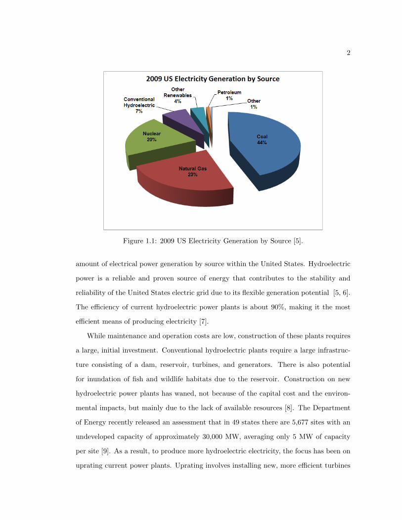
Shown in Figure 1.1, coal, gas, and nuclear dominate the United States energy supply,

comprising 87 percent of the national energy supply [5]. Thus, in order for individual

states to meet their targets, the installation of renewable energy technologies must in-

crease over the next decade. The current technologies that are mainly being used to

meet these target percentages include traditional hydropower, wind, and solar.

Traditional hydropower is a proven power source within the United States that, in the

early part of the 20th century, generated nearly half of the nation’s electricity. In 2009,

this figure has drastically dropped to only 7 percent, but it is still the fourth highest

2

Figure 1.1: 2009 US Electricity Generation by Source [5].

amount of electrical power generation by source within the United States. Hydroelectric

power is a reliable and proven source of energy that contributes to the stability and

reliability of the United States electric grid due to its flexible generation potential [5, 6].

The efficiency of current hydroelectric power plants is about 90%, making it the most

efficient means of producing electricity [7].

While maintenance and operation costs are low, construction of these plants requires

a large, initial investment. Conventional hydroelectric plants require a large infrastruc-

ture consisting of a dam, reservoir, turbines, and generators. There is also potential

for inundation of fish and wildlife habitats due to the reservoir. Construction on new

hydroelectric power plants has waned, not because of the capital cost and the environ-

mental impacts, but mainly due to the lack of available resources [8]. The Department

of Energy recently released an assessment that in 49 states there are 5,677 sites with an

undeveloped capacity of approximately 30,000 MW, averaging only 5 MW of capacity

per site [9]. As a result, to produce more hydroelectric electricity, the focus has been on

uprating current power plants. Uprating involves installing new, more efficient turbines

3

and generators to produce more power from the same resource. Since 1978, more than

1,600 MW of power capacity has been added to the United States electrical grid.

Thus, in order for the United States to increase the amount of electricity generated

by water, new technology is needed to harness the power of the waves, rivers, tides,

and ocean currents. Marine hydrokinetic devices, or MHK, are the answer. Marine hy-

drokinetic devices generate electricity by capturing the kinetic energy of a moving water

source and converting this energy into electrical energy. These turbines are categorized

into two different devices: wave and current. Wave devices typically operate either by

using the oscillations of a wave to drive a hydraulic fluid through a generator or by

trapping air and forcing it through a wind turbine. Tidal and current devices operate

similarly to wind turbines, but use water as the working fluid. Using tidal flow or cur-

rents as a power source is very desirable as they are predictable and have a high energy

density. To understand where to initiate designs of horizontal-axis marine hydrokinetic

turbines, it is important to study their predecessors.

1.1 Wind Turbine Designs

Wind turbines have proven themselves as a viable source of renewable energy; in 2009,

they generated 74 million megawatt-hours, or nearly 2% of the electricity within the

United States [5]. Through accurate siting studies and advanced wind forecasting com-

bined with increased turbine capacities, the annual energy generated from wind turbines

is increasing yearly.

Displayed in Table 1.1 are four sample turbines: two small-scale and two large-scale,

as defined by their power rating. Small-scale turbines, such as the Southwest Windpower

Skystream 3.7 shown in Figure 1.2a, are typically used for off-grid applications or to

contribute to supplemental power for homes and businesses. For simplicity, most small-

scale turbines utilize a direct-drive, permanent-magnet generator. To control their power

output, small turbines utilize a simple approach through either passive stall or passive

4

Table 1.1: Specifications of existing wind turbines.

Small-Scale Turbines Large-Scale Turbines

Skystream 3.7 Bergey Excel GE 1.5sl Gamesa G87Number of Blades 3 3 3 3

Rotor Diameter (m) 3.72 7 77 87Hub to Tip Ratio - - 0.026 0.023

RPM 300 350 18.5 19Tip-Speed Ratio 4.5 10.7 6.21 5.77

Rated Power (kW) 2.4 10 1500 2000Power Control Passive Stall Passive Furling Variable Pitch Variable Pitch

furling. These turbines operate at much higher revolutions per minute, or RPM; however,

due to their small diameters, as compared to large-scale turbines, their tip-speed ratios

are still rather low. As defined in Equation 1.1, the rotor tip-speed ratio, λ, is the ratio

of the tip velocity divided by the inflow velocity:

λ =Ωr

U∞. (1.1)

While small-scale and large-scale wind turbines are similar in theory, they differ

in application. Large-scale turbines, such as the GE 1.5MW wind turbine shown in

Figure 1.2b, are used in the utility sector to produce power for the national electric grid.

These turbines contain a gearbox to increase the revolutions per minute of the drive

shaft before being transferred to the rotor of an asynchronous generator. A gearbox is

used to maintain an appropriate shaft speed on both the rotor side and the generator

side of the drivetrain. To control their power output, nearly all large-scale wind turbines

utilize an active pitch control system. While the exact aspect ratio is proprietary to each

company, wind turbines typically have long, thin blades to minimize blockage effects and

increase their overall efficiency.

Wind turbines have a major advantage of being able to extract renewable energy

from the kinetic flow of wind; however, they are not without their disadvantages. Since

power extracted is related to the wind speed cubed, small variables in wind speed greatly

5

(a) Skystream 3.7 Wind Turbine (b) GE 1.5 MW Wind Turbine

Figure 1.2: Example Wind Turbines [10, 11].

impact the power production of a turbine. At a wind farm, there is a wide range of wind

speeds. Thus, turbines must be designed to operate in all of these conditions. This can

impact the overall efficiency of the turbine and reduce the power factor of the turbine.

Additionally, the aerodynamic noise of the turbine blades causes negative environmental

effects. As stated by Burton, ”the aerodynamic noise generated by a wind turbine

is approximately proportional to the fifth power of the tip speed” [12]. This causes

designs to optimize to lower rotational speeds when the wind speed is low to limit noise

pollution. Lastly, groups have protested the construction of wind turbines since they

alter the natural landscape of an area. Perhaps one of the more prominent groups, the

Alliance to Protect Nantucket Sound, has been directly protesting the construction of

the offshore Cape Wind project located within the Nantucket Sound. While not opposed

to wind energy, they are opposed to the construction of this wind farm for numerous

reasons. One of their primary concerns is the degradation of the view from various

locations surrounding the proposed wind farm [13].

Marine hydrokinetic turbines are a viable option to limit these concerns. The current

resources are more consistent and predictable, hence facilitating resource-driven designs

to optimize the power extraction. Also, since MHK turbines operate in a submerged

environment, noise pollution’s effect on nearby residents is of less concern. For completely

6

submerged applications, they post no threat to the seascape of an area. For designs that

utilize a surface piercing structure, this structure will be a fraction of the height of

their offshore wind counterparts. Discussed in more depth later, noise generated from

cavitation can lead to noise pollution in the underwater environment. However, they are

not without their own unique set of problems that are discussed in the next sections.

1.2 Marine Hydrokinetic Turbines

While there are multiple different types of marine hydrokinetic turbines, this thesis will

only focus on unducted horizontal-axis turbines. While they are comprised of multiple

ducted turbines, barrage systems are discussed because they are comprised of tidal-driven

horizontal-axis turbines.

1.2.1 Barrage

Tidal barrage systems operate much like conventional hydropower; they require a head

differential to create hydrostatic pressure to drive water through a set of turbines. As

such, they require a dam to be built across a bay or estuary that experiences a large tidal

range. Additionally, since the existing bay becomes the reservoir to contain the water,

the inundation of wildlife habitats is greatly reduced as compared with conventional

hydropower plants. This technology is useful in tidal locations where there is a large

height difference between high and low tide. As the tide flows in and the water level

rises, sluice gates are opened in the barrage to allow the water to flow into a basin. Once

the high tide mark is reached, the sluice gates are closed, and the water is forced through

a set of turbines as it drains [14]. The power available in a tidal barrage is a function

of basin area, water density, gravity, and head in the form

P =1

2ρAgh2 . (1.2)

7

Figure 1.3: Rance tidal barrage power plant [15].

One such barrage is the Rance Tidal Power Station in France, shown in Figure 1.3 [15].

This is the largest operating tidal barrage plant in the world with a generating capacity

of 240 MW [14]. Since power is related to the square of height, this power plant operates

their turbines in reverse as pumps during certain tides to create a larger head differential.

This results in the plant’s ability to extract more power for a long time period.

1.2.2 In-stream: Tidal and Current

The design of horizontal-axis marine hydrokinetic turbines have initiated from the lessons

learned from similar wind turbines. Initial designs and design concepts tried to maintain

tip-speed ratios of six to seven. However, designs have begun to converge to lower tip-

speed ratios to limit surface cavitation, which is discussed later. Initial MHK blade

designs also used high aspect ratio, or long and thin, blades that proved unfeasible for

MHK operation due to the increased loading underwater.

In-stream horizontal-axis turbines operate using the current produced by the near

steady flow of water in rivers or the oscillating motion of tidal flows. At first, they

appear to be simply wind turbines that have been placed underwater. However, this

is not the case. Marine hydrokinetic turbines have their own unique set of challenges

that differ greatly from wind turbines as a direct result of their operating environment.

Due to greatly increased maintenance costs, these turbines must be designed in a robust,

8

yet simple manner to reduce the frequency of scheduled maintenance. Bearings, seals,

generators, and structures must be designed and engineered for operation in the harsh

marine environment. Coatings are typically applied to blades and structures to prevent

performance drops due to biofouling that can change the operational characteristics of

the turbine.

Table 1.2: Specifications of existing marine hydrokinetic turbines.

Small Scale Turbines Large Scale Turbines

Verdant River Star SeaGen DeepGenNumber of Blades 3 4 2 3

Rotor Diameter (m) 5 6.1 16 18Hub-to-Tip Ratio 0.151 0.101 0.113 0.138

Aspect Ratio 10.4 10.8 6 10.7RPM 32 12 14.3 -TSR 4.19 - 5 -

Rated Power (kW) 56 50 600 1000Mooring Pile Mounted Floating Tethered Pile Mounted Anchored to Seabed

Power Control Passive Stall Passive Stall Variable Pitch Variable Pitch

Unlike wind turbines, as evidenced by the data in Table 1.2, the designs for marine

current turbines have not yet converged to an optimal design. This can be attributed

primarily to the infancy of the technology and the uncertainty of actual performance.

As a result, there are many distinct areas that need to be studied to improve the design

of marine hydrokinetic turbines.

To capture as much energy as possible and minimize undesired forces on the blades,

both current and tidal turbines typically have the ability to either yaw the entire turbine

into the flow or pitch the blades as the flow direction changes with the ebb and flow of the

tides. Additionally, the hub-to-tip ratio, which is the ratio of hub diameter compared

to the rotor diameter, is much larger. This is a result of the need to withstand the

increased loads on the blades as a direct result of water density relative to air. Due to the

proprietary nature of resource assessments for these turbines, only a partial comparison

of the tip-speed ratios among these sample turbines can be completed.

9

Furthermore, there are numerous options for mounting and securing these turbines.

The Verdant and SeaGen turbines both utilize a pile-mounted design [16]. The pile-

mounted SeaGen Tidal Turbine, which is currently in operation in the Strangford Loguh

in Northern Ireland, can be seen in Figure 1.4. This turbine uses a variable pitch variable

speed design to extract 1.2 MW of power at a rated flow speed of 2.4 m/s [16]. It features

two counter-rotating turbines to balance the rotational inertia on it’s mooring.

Figure 1.4: SeaGen tidal current turbine [16].

Another approach is with a turbine that is suspended from a floating platform. An

example of this approach can be seen in the conceptual design of the River Star turbine

by Bourne Energy shown in Figure 1.5 [17]. Both the Verdant and River Star turbines

utilize a passive yaw approach to align itself with the flow. Since the direction of the

tidal flow at the SeaGen turbine are consistent and fully reversible, this turbine includes

the ability to pitch its blades 180 degrees to maximize its energy capture.

10

Figure 1.5: The River Star current turbine [17].

1.3 Tidal Flows

In order understand how power is extracted from the tides, an explanation of the tides

themselves is necessary. The tides experienced on Earth are a direct result of the grav-

itational effects of the Sun and moon. Newton’s Law of Universal Gravitation states

that the attractive force is “directly proportional to the product of the two masses and

inversely proportional to the square of the distance between their centers [18].” Thus,

even though the Sun is much larger than the moon, it has less of an effect on the tides

because it is much further away.

On the Earth, there are always two tidal bulges. One is a direct result of the moon’s

gravitational effect on the Earth, which is the largest on the side that faces the moon.

As a result, the water on this side of the Earth is attracted to the moon and a bulge is

formed. The second bulge is located on the side of the Earth farthest from the moon.

On this side, the moon’s gravitational effect is at a minimum and the inertial effects,

which are caused by the Earth revolving around the sun dominate. These bulges can be

seen in Figure 1.6.

The frequency of tides is dictated by the length of the lunar day. The lunar day is

the time it takes for a specific point on the Earth underneath the moon to rotate to the

11

Figure 1.6: Tidal bulges on the Earth [19].

exact same location. On Earth, the lunar day is 24.83 hours. Due to the two bulges, each

location on the earth experiences two high and two low tides per day. Also, during each

lunar month, two sets of spring tides and two sets of neap tides occur. Spring tides are a

result of the additive effect of the Sun’s gravitational pull, and this creates significantly

larger tidal ranges. Neap tides occur when the moon and sun are at right angles to each

other resulting in moderate tides [19]. This consistent, predictable flow yields a large

energy capture potential that has led to the development of tidal hydrokinetic turbines.

1.4 Resource Assessment

To determine if a marine hydrokinetic turbine is appropriate at a site, a study of the

resource must be performed. This is done by gathering current data at a location and

creating plots of the flow probability. Typically, Weibull distributions are used because

they have been proven as a valuable tool for wind turbine designers. The Weibull proba-

bility density function is shown below in Equation 1.3, and it equates the flow probability

at each flow speed [20]:

p(U) =

(k

c

)(U

c

)k−1exp

[−(U

c

)k]. (1.3)

These distributions utilize two parameters: a scale parameter c and a shape parame-

ter k. The scale parameter is the site characteristic speed, and it is related to the average

12

flow speed. The shape parameter is related to the standard deviation of flow speeds at

the site; the lower the value of k, the greater variability about the mean [12].

Additionally, the resource assessment involves binning of flow speeds, where a range of

flow speeds are lumped into a bin to estimate the number of yearly hours of operation at

that flow speed. This yearly operation data is valuable for the annual energy production

economic assessment discussed in the next section.

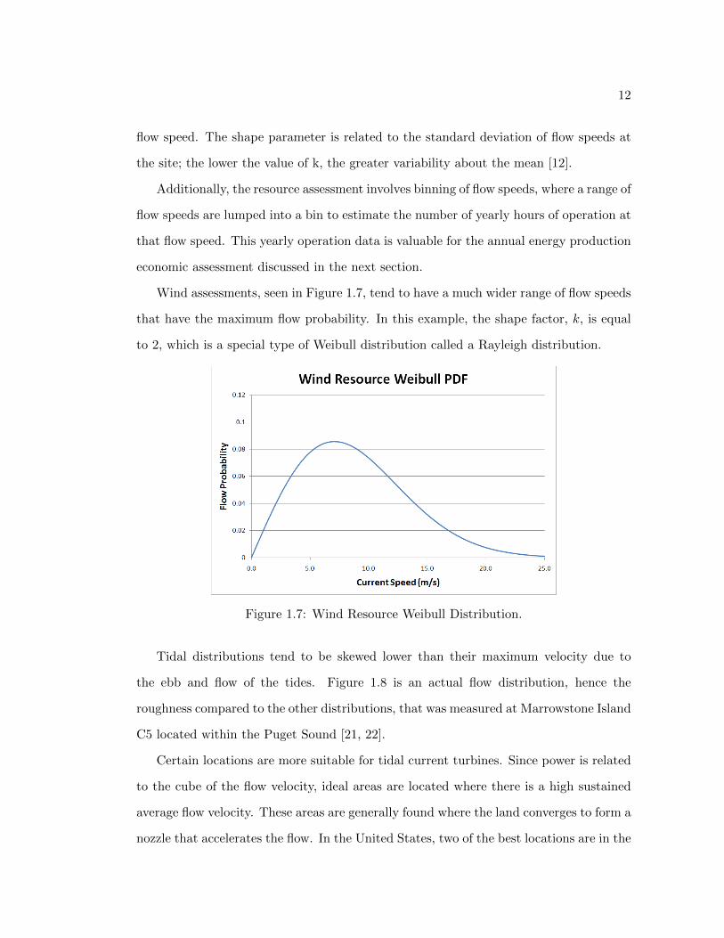
Wind assessments, seen in Figure 1.7, tend to have a much wider range of flow speeds

that have the maximum flow probability. In this example, the shape factor, k, is equal

to 2, which is a special type of Weibull distribution called a Rayleigh distribution.

Figure 1.7: Wind Resource Weibull Distribution.

Tidal distributions tend to be skewed lower than their maximum velocity due to

the ebb and flow of the tides. Figure 1.8 is an actual flow distribution, hence the

roughness compared to the other distributions, that was measured at Marrowstone Island

C5 located within the Puget Sound [21, 22].

Certain locations are more suitable for tidal current turbines. Since power is related

to the cube of the flow velocity, ideal areas are located where there is a high sustained

average flow velocity. These areas are generally found where the land converges to form a

nozzle that accelerates the flow. In the United States, two of the best locations are in the

13

Figure 1.8: Tidal Resource Probability Distribution [21, 22].

Puget Sound and the Bay of Fundy. The Admiralty Inlet and Tacoma Narrows areas

within the Puget Sound offer the best potential at this location for power generation

with a mean power density of 0.8 kW/m2 and 1.1 kW/m2 and a mean power potential

of 230MW and 65 MW, respectively [23]. The location of Admiralty Inlet can be seen

in Figure 1.9 [24].

The Bay of Fundy has the largest tides in the world; the range of sea level height

change can be more than 16 meters. As a result, a significant amount of water flows in

and out of this passage daily, thus creating an immense energy potential [25]. Figure 1.10

shows the magnitude of the sea level change by showing a boat that would normally float

sitting on the bottom due to the low tide [26]. Resource estimates of the Minas Passage,

shown in Figure 1.11, located within the Bay of Fundy have predicted a mean power

density of 6.036 kW/m2 and a mean potential power of 1.9 GW [27, 28]. For select US

resources, the National Oceanic and Atmospheric Administration provide detailed tidal

and current predictions at no cost to the consumer [29].

In Europe, there are many excellent locations for hydrokinetic energy extraction.

The SeaGen turbine is located in the Strangford Lough that is an inlet from the Irish

Sea [16]. As seen in Figure 1.12, this location forms a natural nozzle that increases

14

Figure 1.9: Puget Sound tidal resource [24].

Figure 1.10: Sea level change in the Bay of Fundy [26].

the current velocity. Another potential site is in the Sound of Islay in Scotland where

Scottish Power Renewables recently got approval to install ten turbines. Not only is the

current resource excellent in this area, but the required grid capacity is also available at

this location [30].

15

Figure 1.11: Bay of Fundy tidal resource [28].

Figure 1.12: Location of SeaGen tidal turbine in the Strangford Lough [16].

16

1.5 Power Available

River and tidal currents offer an immense energy capture potential with horizontal axis

marine hydrokinetic turbines. The available power within a flow, or the kinetic energy

per unit time, is given by

Poweravail =1

2ρAU3

∞ . (1.4)

However, the actual power extracted by a turbine is less than the available power. To

start, the determination of the power extracted in a rotor disc area is derived from the

Actuator Disc Model. As shown in Figure 1.13, the Actuator Disc approach models the

flow as a stream tube that expands as it passes through the rotor plane [12]. It assumes

that the flow is only in one direction, the fluid is inviscid and irrotational, the rotor itself

does not rotate, and the flow is steady through the rotor plane. To determine a turbine’s

power output, a momentum balance must be performed.

Figure 1.13: Wind turbine stream tube [12].

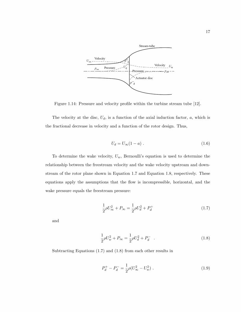
Figure 1.14 shows the fluid through the rotor disc area undergoes a decrease in

velocity, which results in a force due to a change of momentum of the flow that is equal

to [12]

Force = (P+d − P

−d )Ad = (U∞ − Uw)ρAdUd . (1.5)

17

Figure 1.14: Pressure and velocity profile within the turbine stream tube [12].

The velocity at the disc, Ud, is a function of the axial induction factor, a, which is

the fractional decrease in velocity and a function of the rotor design. Thus,

Ud = U∞(1− a) . (1.6)

To determine the wake velocity, Uw, Bernoulli’s equation is used to determine the

relationship between the freestream velocity and the wake velocity upstream and down-

stream of the rotor plane shown in Equation 1.7 and Equation 1.8, respectively. These

equations apply the assumptions that the flow is incompressible, horizontal, and the

wake pressure equals the freestream pressure:

1

2ρU2∞ + P∞ =

1

2ρU2

d + P+d (1.7)

and

1

2ρU2

w + P∞ =1

2ρU2

d + P−d . (1.8)

Subtracting Equations (1.7) and (1.8) from each other results in

P+d − P

−d =

1

2ρ(U2

∞ − U2w) . (1.9)

18

Substituting Equations (1.6) and (1.9) into Equation 1.5 results in

1

2ρ(U2

∞ − U2w)Ad = (U∞ − Uw)ρAdU∞(1− a) . (1.10)

Solving for Uw, the wake velocity is

Uw = (1− 2a)U∞ . (1.11)

By comparing Equations (1.6) and (1.11) with each other, it can be concluded that

half of the total decrease in flow velocity occurs before the rotor disc and half occurs

after the rotor disc [12]. To determine the force on the turbine, Equations (1.5), (1.6)

and (1.11) are combined to form

Force = (P+d − P

−d )Ad = 2ρAdU

2∞a(1− a) . (1.12)

The power extracted by the actuator disc is “the rate of work done by the force”,

which is equal to the force multiplied by the disc velocity where [12]

Power = ForceUd = 2ρAdU3∞a(1− a)2 . (1.13)

The power that the turbine can extract from its working fluid is limited by an effi-

ciency factor, and this is designated by the power coefficient, CP . The power coefficient

can be described as the actual power extracted by the turbine divided by the total power

available, Equation 1.4, and thus

CP =PoweractualPoweravail

=Poweractual

12ρAdU

3∞

. (1.14)

By combining Equation 1.13 with Equation 1.14 for the Actuator Disc, the expression

for CP can be reduced to the form

CP = 4a(1− a)2 . (1.15)

19

To find the maximum power coefficient, the optimal value for a must be determined

by finding the roots of the derivative of Equation 1.15, where

dCPda

= 4(1− a)(1− 3a) = 0 . (1.16)

This results in a value of a = 13 , and thus

CPmax =16

27= 0.593 . (1.17)

The Betz limit, as displayed in Equation 1.17, is the maximum possible power co-

efficient of any horizontal-axis turbine [12]. The Betz limit is validated through the

application of conservation of mass to the stream tube. As shown in Equation 1.18,

as the velocity of the flow decreases, the cross sectional area of the stream tube must

increase:

ρA∞U∞ = ρAdUd = ρAwUw . (1.18)

Ergo, the Betz limit is due to the fact that the stream tube must expand before it

reaches the actuator disc; as a result, the cross section of the stream tube where the fluid

is at the freestream velocity is smaller than the area of the disc [12]. To date, no wind

or marine hydrokinetic turbine has been able to exceed this limit. This expansion of the

stream tube and decrease in velocity as the fluid moves towards the rotor plane can be

seen previously in Figure 1.14.

In practice, the maximum value of the power coefficient varies as a function of the

number of blades and the tip-speed ratio of the turbine. Wilson developed a relationship,

shown in Equation 1.19, between the maximum achievable power coefficient for turbines

with an optimum blade shape, but with a specific number of blades and drag [31].

CPmax =16

27λ(λ+

1.32 + (λ−820 )2

B23

)−1 − 0.57λ2

ClCd

(λ+ 12B )

(1.19)

20

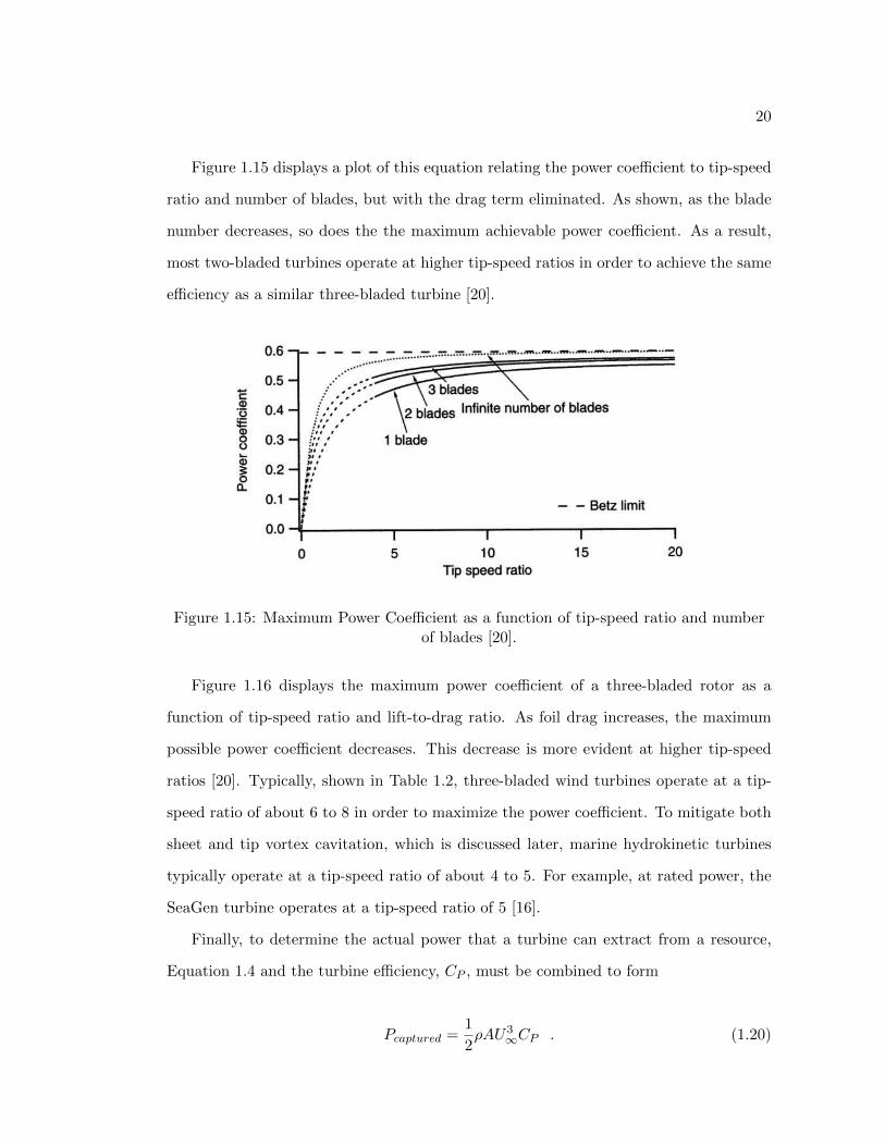
Figure 1.15 displays a plot of this equation relating the power coefficient to tip-speed

ratio and number of blades, but with the drag term eliminated. As shown, as the blade

number decreases, so does the the maximum achievable power coefficient. As a result,

most two-bladed turbines operate at higher tip-speed ratios in order to achieve the same

efficiency as a similar three-bladed turbine [20].

Figure 1.15: Maximum Power Coefficient as a function of tip-speed ratio and numberof blades [20].

Figure 1.16 displays the maximum power coefficient of a three-bladed rotor as a

function of tip-speed ratio and lift-to-drag ratio. As foil drag increases, the maximum

possible power coefficient decreases. This decrease is more evident at higher tip-speed

ratios [20]. Typically, shown in Table 1.2, three-bladed wind turbines operate at a tip-

speed ratio of about 6 to 8 in order to maximize the power coefficient. To mitigate both

sheet and tip vortex cavitation, which is discussed later, marine hydrokinetic turbines

typically operate at a tip-speed ratio of about 4 to 5. For example, at rated power, the

SeaGen turbine operates at a tip-speed ratio of 5 [16].

Finally, to determine the actual power that a turbine can extract from a resource,

Equation 1.4 and the turbine efficiency, CP , must be combined to form

Pcaptured =1

2ρAU3

∞CP . (1.20)

21

Figure 1.16: Maximum Power Coefficient of a three-bladed turbine as a function oftip-speed ratio and lift to drag ratio [20].

1.6 Annual Energy Production

The calculation of annual energy production, AEP, is performed through an integration

of the turbine power curve and the resource assessment. AEP calculations are performed

as part of the economic assessment to determine the profit potential of an undeveloped

site. As explained by Burton [12], this calculation combines the binned flow speed

distribution with the power curve such that

Energy =

i=n∑i=1

H(Ui)P (Ui) . (1.21)

This equation states that the total energy produced is a sum of the total number

of hours in each wind bin, H(Ui), multiplied by the power output, P (Ui) at that wind

speed, and then summed over all the wind bins. This annual energy production of the

turbine can then be used to estimate yearly profits from power generation, and it can be

used in economic modeling of the turbine design and siting.

22

1.6.1 Capacity Factor

The capacity factor, CF , of a turbine is very important in turbine design and site selec-

tion. It is a ratio of actual output of the turbine divided by the power it would have

produced if it were operating at its full capacity during that time period with consider-

ation of the resource at the site [32]. Table 1.3 lists the 2009 capacity factors for various

energy sources [33]. It is important to note that those with the highest capacity factors,

coal and nuclear, are typically operated at full capacity to provide base load power to the

grid. Conversely, conventional hydropower is easily dispatchable at the request of power

grid operators when demand increases, resulting in a lower capacity factor. Lastly, it is

anticipated, based on the typical current probability, that the capacity factor for marine

hydrokinetic turbines will be higher than wind based on their specific design for a more

consistent resource.

Table 1.3: Summary of Capacity Factors by Energy Source [33].

Energy Source 2009 Capacity Factor

Nuclear 89Geothermal 85

Coal 85MSW Landfill Gas 83

IGCC 80Biomass 75

CCGT 70Hydropower 43

Wind - Offshore 42Wind - Onshore 39

Solar Thermal 31Solar PV 22

Combined Turbine 10

1.7 Turbine Power Generation

For a turbine to produce power, the linear motion of the flow is converted to a rotational

motion to drive a generator. This is performed by using lifting surfaces to create a lift

23

force on the blade. Determination of this lift force is calculated using Newton’s first and

third laws through the application of momentum conservation. The first law states that

there must be a conservation of momentum within the flow. This means that as the

airfoil bends the fluid flow, there is a force acting upon the fluid. The third law states

that for every force there is an equal and opposite reaction force. A force is defined

as the rate of change of momentum. To maintain conservation of momentum, as the

airfoil creates a downward force on the fluid, the fluid exerts an equal and opposite force

upward in the form of lift [34].

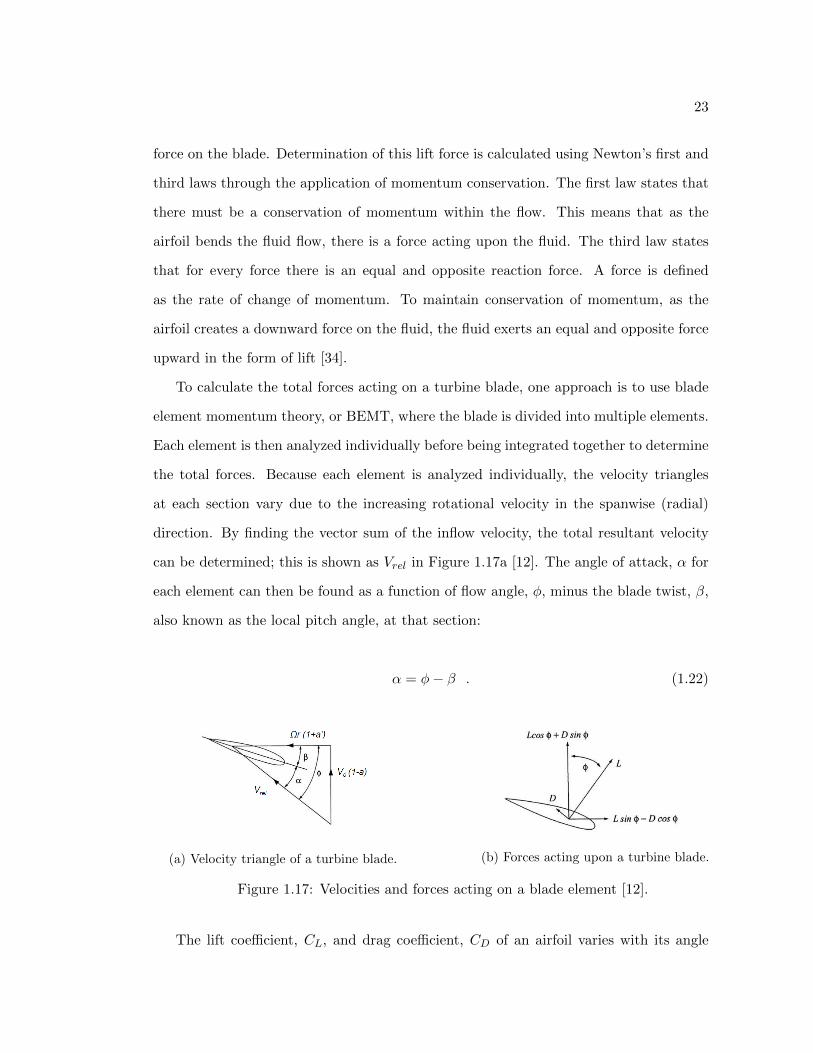
To calculate the total forces acting on a turbine blade, one approach is to use blade

element momentum theory, or BEMT, where the blade is divided into multiple elements.

Each element is then analyzed individually before being integrated together to determine

the total forces. Because each element is analyzed individually, the velocity triangles

at each section vary due to the increasing rotational velocity in the spanwise (radial)

direction. By finding the vector sum of the inflow velocity, the total resultant velocity

can be determined; this is shown as Vrel in Figure 1.17a [12]. The angle of attack, α for

each element can then be found as a function of flow angle, φ, minus the blade twist, β,

also known as the local pitch angle, at that section:

α = φ− β . (1.22)

(a) Velocity triangle of a turbine blade. (b) Forces acting upon a turbine blade.

Figure 1.17: Velocities and forces acting on a blade element [12].

The lift coefficient, CL, and drag coefficient, CD of an airfoil varies with its angle

24

of attack. The lift and drag forces on each element of length dr are functions of the

dynamic pressure multiplied by the local chord length, C, and lift and drag coefficients,

respectively, in the form [12]

dL =1

2ρV 2

relCLCdr (1.23)

and

dD =1

2ρV 2

relCDCdr . (1.24)

Next, to calculate the thrust, dT , and torque, dQ, produced at each section, a coor-

dinate transformation is performed on the lift and drag forces, shown in Figure 1.17b,

where

dT = dLcosφ+ dDsinφ (1.25)

and

dQ = (dLcosφ− dDsinφ)dr . (1.26)

It is important to note that the lift and drag forces always act normal and parallel

to the chord line, respectively, and the thrust and torque always act normal and parallel

to the rotor plane, respectively.

Finally, the total power is found by multiplying the total torque produced by each

of the turbine blades by the angular velocity, Ω, such that

Power = QΩ . (1.27)

25

1.7.1 Foil Selection

Because the lift and drag coefficients play such an integral role in the turbine perfor-

mance, proper foil selection is important. In making that determination, three values

are typically studied: the maximum lift coefficient, CLmax , the lift-to-drag ratio, CLCD

,

and the minimum pressure coefficient, CPmin . A high CLmax is desired to maximize

the lift produced by the blade. As shown previously, the more lift that is produced,

the more torque that can be generated resulting in increased power. As evidenced in

Figure 1.16, the higher the CLCD

the greater the power coefficient at various tip-speed ra-

tios [20]. Lastly, unlike airfoils used for wind turbine airfoils, the value of the minimum

pressure coefficient, or CPmin , is critical to mitigate surface cavitation, discussed in the

next section.

It is important to find foils that contain these desirable properties to design optimal

hydrokinetic turbine blades. Many wind turbines utilize multiple airfoils within one

blade design to optimize their varying properties at the different operating regions of

the blade. A trade-off analysis must also be performed for structural considerations

and manufacturing constraints. This typically results in larger root sections, in both

thickness and chord length, to reduce bending stresses. Also, due to both manufacturing

limitations and load conditions, modifications are often made to sharp trailing edges.

1.8 Cavitation

One of the major concerns of marine hydrokinetic turbine blade design that can directly

impact the power generated is cavitation. Cavitation occurs when the local pressure is

lower than the vapor pressure of the liquid, resulting in small bubbles or vapor clouds [35].

The vapor pressure is defined as the pressure that the liquid vaporizes, and it is a function

of the liquid type and temperature [36].

Cavitation noise and damage are caused by the collapse of these small bubbles. Once

the bubble has moved further downstream to a region with a local pressure higher than

26

the vapor pressure, the bubble collapses. This collapse results in a high localized pressure

caused by the immediate filling of the cavity by the surrounding fluid [37].

There are two types of cavitation, surface and vortex. Surface cavitation is of primary

concern as that it can directly impact the operational performance of the turbine blade.

This form of cavitation can result in a loss of lift paired with an increase in drag, thus

reducing the lift-to-drag ratio. As discussed previously, power is produced by using

airfoils to produce lift. Without adequate lift, power production is directly affected.

Vortex cavitation does not impact the blade’s performance. However, both have the

potential to cause unwanted noise and to impact the lifetime of downstream structures

if the bubbles collapse on the surface of these structures [38].

1.8.1 Surface

To determine if surface cavitation will occur, a comparison between the minimum pres-

sure coefficient, Cpmin , of the airfoil and the cavitation number must be performed. The

pressure coefficient is defined as the difference in local pressure and free stream pressure

divided by the dynamic pressure in the form [39]

Cp =PL − P∞

12ρU

2∞

. (1.28)

For surface cavitation, the cavitation number is defined as

σcavitation =P∞ − Pvap

12ρU

2∞

. (1.29)

where

P∞ = Patm + ρgh (1.30)

For cavitation free operation

27

σcavitation > −Cpmin . (1.31)

An image of surface cavitation can be seen in Figure 1.18. Over time, surface cav-

itation can result in surface pitting due to bubble collapse on the surface, which will

negatively impact the turbine’s operation [38]. This pitting is caused by the local pres-

sure developed during the bubble collapse, which can impart high stress levels that

exceed the resistance of the blade material [36]. This pitting yields an increase in surface

roughness that influences the turbulence within the boundary layer around the airfoil.

As stated by Arndt, “the major influence of the roughness is an increased turbulence

intensity” [38]. This impacts the operational characteristics by changing the properties

of the airfoil, and, subsequently, the lift-to-drag ratio of the airfoil. This loss of lift is a

result of an induced stall of the airfoil caused by the effects of surface cavitation.

Figure 1.18: Surface cavitation on NACA 4412 foil [40].

Surface roughness, which can be a result of biofouling of the blades, directly af-

fects cavitation inception. As discussed by Tada, surface roughness can be categorized

into either isolated or distributed. Isolated irregularities are more harmful because they

28

cause ”high local velocities, low pressures, and turbulence in the neighborhood of the

projection” [41]. Similarly, distributed roughness impacts velocity, pressure, and turbu-

lence, but throughout the boundary layer. He concludes that isolated roughness is more

of a concern for surface cavitation inception due to the more severe localized pressure

reduction [41].

Conventional hydropower has dealt with the effects of cavitation erosion, mostly with

varying levels of success [42]. For marine hydrokinetic devices, surface cavitation can be

mitigated by increasing the depth, thus increasing the cavitation number, and by proper

airfoil selection. However, depending on the resource, could result in a lower current

velocity and impact power production of the turbine.

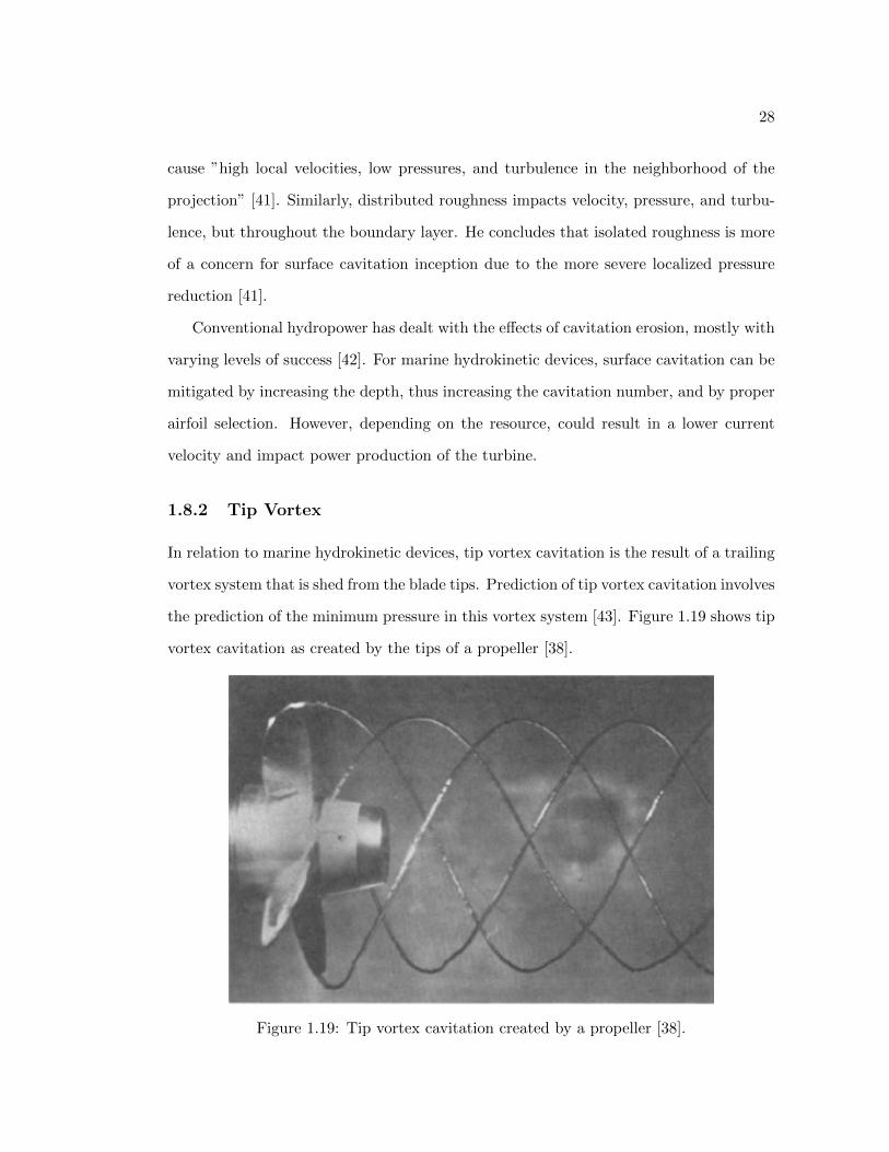
1.8.2 Tip Vortex

In relation to marine hydrokinetic devices, tip vortex cavitation is the result of a trailing

vortex system that is shed from the blade tips. Prediction of tip vortex cavitation involves

the prediction of the minimum pressure in this vortex system [43]. Figure 1.19 shows tip

vortex cavitation as created by the tips of a propeller [38].

Figure 1.19: Tip vortex cavitation created by a propeller [38].

29

To determine the cavitation number, tip vortex inception prediction has been reduced

to the form

σi = KC2LRe

m . (1.32)

As discussed by Arndt, the value of m is accepted to be 0.4. The value of K varies

due to a secondary effect caused by variations in vortex roll-up for various blades. As a

result of experimental validation, K varies from 0.035 to 0.073 for airfoils with an elliptic

planform, depending on the airfoil shape. Differences with K can be attributed to the

methods to correct for water quality, blockage effects, and lift correction values [44].

Additionally, Equation 1.31 holds true to predict tip vortex cavitation free operation

with a slight modification by replacing CPmin of the airfoil with the minimum pressure

coefficient of the vortex, Cp,vortex in the form [45]

σi > −Cp,vortex . (1.33)

The damage of downstream structures caused by tip vortex cavitation has been stud-

ied extensively with regards to ship rudders. Damage to the rudder is frequently caused

by cavitation produced by the propeller and then transported downstream to the rudder

where the bubbles collapse and cause erosion of the surface [46]. The same mechanism for

cavitation damage holds true for marine hydrokinetic turbines causing damage to down-

stream structures through the collapse of bubbles created by cavitation of the turbine

blades.

1.8.3 Cavitation Noise

The noise caused by the collapse of the cavitation bubbles is also of concern, primarily

for environmental reasons. The noise is a direct result of the pressure change caused by

collapse of cavitation bubbles. In conventional hydropower, cavitation has been studied

extensively. Detection of cavitation is monitored by detecting an increase in noise within

30

the medium to high frequency ranges, 15-100 kHz [47]

In a report by Wang et al., a test on a horizontal axis turbine model was performed in

the emersion cavitation tunnel at Tyne University. They concluded that the noise levels

in the frequency range of 5-30 kHz increase with the intensities of the tip and unstable

cloud cavitations [48]. Currently, there are no standards that limit the noise a marine

hydrokinetic turbine can produce, but the impacts of cavitation must be understood to

mitigate future concerns.

1.9 Environmental Impacts

Numerous environmental concerns must be taken into account when installing and op-

erating marine hydrokinetic devices. However, most of these assessments are based on

estimated impacts rather that measured impacts [49]. From cradle to grave, marine hy-

drokinetic devices have the potential to impact their environment, both positively and

negatively.

1.9.1 Installation and Decommissioning Effects

Installation of marine hydrokinetic devices pose plausible environmental impacts. Sedi-

ment removal and propagation can result in a loss of habitat for local marine organisms.

Water turbidity, due to suspended sediments and possibly contaminants, can effect the

local water quality of the site. The equipment needed for turbine installation and removal

also can impact local organisms or impact migratory routes of marine organisms [50].

Noise levels during the installation of moorings and anchoring devices, as estimated by

the Minerals Management Service, will likely exceed threshold values that are set to pro-

tect fish and marine mammals [51]. Additionally, noise generated from ships and their

equipment during installation and decommissioning is also a concern [49].

Similar to installation, decommissioning effects pose similar risks to the environment.

Noise and water quality can be impacted by the equipment used to remove the turbines.

31

However, one potential positive impact within tropical areas is to simply abandon de-

commissioned devices to let them be converted into artificial reefs [49]. But, this also

prevents future re-use of the site.

1.9.2 Operation and Energy Extraction Effects

Operational effects, both static and dynamic, have the potential to drastically impact the

marine environment. Pressure changes caused by the rotational effects of the blade can

result in harm to marine life. Additionally, as learned from the wind turbine industry,

blade strikes with animals pose a serious environmental risk [49]. However, as shown

previously in Table 1.2, marine turbines operate at drastically slower rotor speeds as

compared to their wind counterparts. Additionally, most studies on impacts to marine

life have been performed on sites that use conventional hydroelectric plants. These

plants operate at 600-700 RPM, and marine animals have little opportunity to avoid

these turbines [52]. As a result, experts have estimated that marine animals have a low

chance of blade strike with open tidal turbines due to an increased ability to avoid the

turbine rotor [53]. Figure 1.20 explains that for horizontal axis turbines, the critical strike

zone is the area where the blades have a high linear velocity combined with no means for

the marine animal to escape [54]. This prediction was confirmed in a study completed

by Hydro Green Energy that stated that only one fish out of 402 showed evidence of

direct physical harm. Even further, this incident was attributed to the balloon tag that

caused the fish to rise to the surface and encounter the turbine in a manner that would

not have occurred naturally [55].

The impact of energy removal from the current flow will reduce local flow velocities;

however, the far-field impact will be much reduced [49]. A study completed in the 1970s

on the Florida Gulf Current concluded that an array of turbines producing 1000 MW of

power would extract roughly 4%, or 25 GW, of the total kinetic energy in the current

over the course of a year. Similarly, if 4 GW of power was extracted from the tidal flow

in the Bay of Fundy, out of a total energy supply of 7 GW, there would be a change in

32

Figure 1.20: Estimated area of a open hydrokinetic turbine for a damaging strike [54].

the tide of less than 10% [51].

Significant reduction in flow velocities in bays and estuaries risks a depreciation of

overall water quality. The main concerns center around sediment transportation, erosion,

and deposition effects as well as dissolved gas content. Changes to flow circulation

can create an increase in these concerns in potential resources. Impacts to sediment

transportation, either an increase or decrease, can alter the bottom profile and local

plant and animal habitats [49].

1.10 Blade Loading

As previously stated, in order to produce rotational power, torque is needed. This torque

is produced along the turbine blade. If not properly designed, the blade can experience

failure through either material cracking or striking the downstream structures.

When Verdant Power installed their first tidal turbine in the East River in New York

City, the anticipated maximum blade loading was not fully understood. As a result,

when the turbine was installed in 2006, the turbine experienced faster than anticipated

currents, and it experienced a blade failure [57]. As shown in Figure 1.21a, a coarse stress

analysis using tetrahedral elements was performed on the original design and predicted

33

(a) Blade Failure (b) FEA Model

Figure 1.21: Verdant Power blade failure [56].

the maximum stress in the location where actual failure occurred [56].

One of the major benefits of turbine blades is that they can be modeled as cantilever

beams. However, basic beam bending methodologies, such as Bernoulli beam theory

and the potential energy method, are too simplified in their commonly published forms.

Modern blades are complex structures of varying twist, chord, and thickness, and many

studies have been performed in the past on similar devices.

Kemper studied tapered beams under large, non-linear deflections [58]. However,

turbine blade deflections are quantified as small deflections, thus linear approximation

of the Bernoulli-Euler equation is appropriate. The Runge-Kutta and predictor correc-

tor methods he outlines to solve the differential equations that solve for deflection are

unnecessary for this analysis.

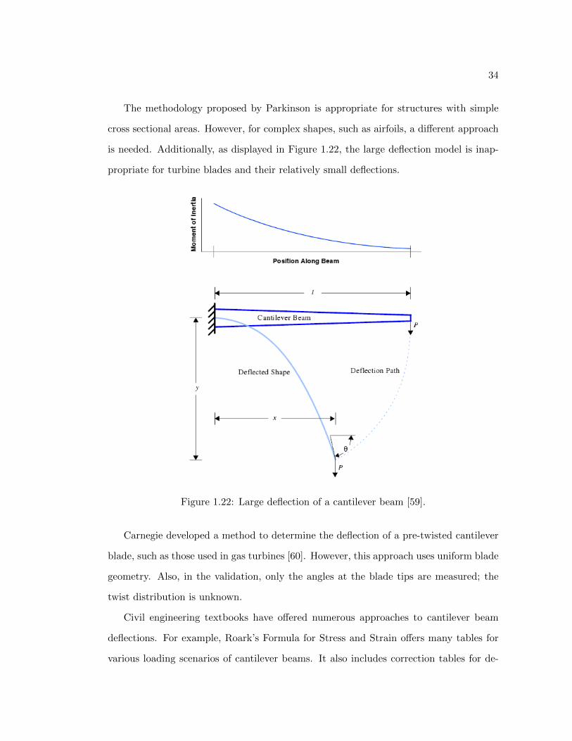
Parkinson went one step further and studied large beam deflections, but without a

lengthy nonlinear analysis. He developed the ellipsoid equation as a function of the ratio

of moment of inertias at the base and tip and found that large, non-linear deflection of

a tip loaded cantilever beam can be found using Equation 1.34 [59]:

y = (0.030432lnIratio + 0.91897)l

√1− x2

l2. (1.34)

34

The methodology proposed by Parkinson is appropriate for structures with simple

cross sectional areas. However, for complex shapes, such as airfoils, a different approach

is needed. Additionally, as displayed in Figure 1.22, the large deflection model is inap-

propriate for turbine blades and their relatively small deflections.

Figure 1.22: Large deflection of a cantilever beam [59].

Carnegie developed a method to determine the deflection of a pre-twisted cantilever

blade, such as those used in gas turbines [60]. However, this approach uses uniform blade

geometry. Also, in the validation, only the angles at the blade tips are measured; the

twist distribution is unknown.

Civil engineering textbooks have offered numerous approaches to cantilever beam

deflections. For example, Roark’s Formula for Stress and Strain offers many tables for

various loading scenarios of cantilever beams. It also includes correction tables for de-

35

flections, angles, and forces for tapered beams with varying distributions [61]. However,

a limitation of this book and other books lie in the fact that in civil engineering, twisted

beams are rarely, if ever, used.

1.11 Current Design Codes

Current blade design methods involve using a blade-element momentum code, such as

WT Perf, to analyze the performance of an initial design. These methods require the

designer to input all of the blade properties, including the chord, twist, and airfoil

distributions [62]. To change and optimize the design, the user must change the input

files and re-run the code, which can be very user and time intensive. Additionally,

the National Renewable Energy Lab (NREL) has many simulation codes to understand

aerodynamics and system dynamics of horizontal-axis wind turbines. However, these

codes require the user to create a separate and unique input file for each turbine design.

Once an acceptable design has been reached, the design can then be run through a

computational fluid dynamics (CFD) solver to produce more accurate performance and

loading data. Typically, CFD is a time and computationally intensive process that is

usually reserved for only a final stage validation. It can take many days to weeks to

generate a computation grid and to run the solver. Thus, it is not practical to use CFD

as an everyday tool. Similar to CFD, a finite-element analysis is performed to determine

the structural behavior of the blade. To develop accurate results, this process is time

intensive and is usually reserved for final stage verification.

NREL has recently released a new design code called HARP Opt [21]. This code

attempts to automate the blade design process by utilizing an optimization routine to

design and analyze thousands of designs to converge to a superior design.

36

1.11.1 HARP Opt Overview

Developed by the National Renewable Energy Laboratory, HARP Opt is a rotor opti-

mization code that utilizes a genetic algorithm to create a population of possible designs

and then converge to the global optimal design [21]. Genetic algorithms operate by cod-

ing the design parameters into genes. Within a population, there are many individuals

where each individual is a unique turbine design. These individuals are then assigned fit-

ness values based on how well they achieve the desired outputs of power production and

annual energy production. The designs are then subjected to natural selection, where

only the best designs, or parents, are allowed to pass through to the next population.

These parents then undergo mating and random mutations in order to populate the next

iteration [63].

To initiate the design process, HARP Opt requires the user to input initial conditions

to which an initial population can be derived. These inputs are comprised of the over-

all turbine geometry, flow and operating conditions, material properties, and dynamic

models. Additionally, upper and lower bounds on the chord length, twist distribution,

and percent thickness are required at five locations along the blade span. Once these

inputs are completed, the initial population is created, and the genetic algorithm is able

to start its optimization. For each discrete individual, a WT Perf input file is auto-

matically created and analyzed. The outputs from this analysis are analyzed, and a

fitness value is created based on the blades performance. Depending on the user defined

algorithm parameters, the code then permits a predetermined number of individuals to

reproduce and mutate to create the subsequent population. This optimization continues

until either the maximum number of iterations is reached or until the difference in the

fitness value is within the predefined tolerance level [64].

Presently, HARP Opt is still in its infancy and is continually being developed. There

are many limitations in the current release of this design code, and this thesis focuses on

improving the optimization to improve the final results.

37

1.11.1.1 Limitations

In the current release of HARP Opt, there are many caveats to its operation. Most

noticeably, the runtime of the code is quite long. This is due to many discrete steps and

is directly influenced by the population size per generation and the number of blade seg-

ments per turbine. Additionally, the sheet cavitation prediction model does not inform

the designer where on the blade cavitation occurs. Instead, the code simply removes that

individual from the population and marks it as an infeasible design. This is undesirable

because perhaps a small change in the blade twist can mitigate the cavitation concerns

and yield an optimal solution.

In its presently released state, the structural design capabilities are rudimentary.

Even though the design code is marketed as a design tool for wind and marine hydroki-

netic blades, the blade cross section is limited to shelled areas with varying thicknesses.

While this may be appropriate for some wind turbines, marine hydrokinetic blades ex-

perience a loading orders of magnitude greater than wind blades due to the density

difference of the working fluid. Thus, a more robust structural design must take place

involving a beam spar that is more commonly used to carry the loads along the blade.

Operating effects on the blade shape are also ignored. During operation, the loadings on

the blade impact the blade pitch– and, subsequently, the lift and drag produced at that

section. In the present version of HARP Opt, these effects are ignored. The next chapter

focuses on overcoming these limitations and improving the structural design capabilities

of HARP Opt.

1.12 Motivation

To develop a robust wind or marine hydrokinetic turbine design software package, un-

derstanding the proper structural behavior is vital to achieve optimal results. It is also

important to understand how this structural behavior impacts the aerodynamic or hy-

drodynamic efficiency of the rotor itself. When these two aspects, the structural design

38

and aerodynamic or hydrodynamic design, are coupled together, the design software

is able to optimize to the superior design by taking into account the cause and effect

relationship between them.

1.13 Scope

This thesis focuses on improving the structural design capabilities of the NREL developed

design code, HARP Opt. These enhancements include more accurate stress models,

a maximum tip deflection constraint, a torsional deflection analysis, and a box spar

design routine. These additions will then be used to improve the hydrodynamic design

of the turbine. By expanding and refining its capabilities, this optimization routine

has the potential to yield superior initial designs. The latter part of the thesis involves

application of this design code to design an in-stream tidal turbine. Only open horizontal-

axis turbines will be studied as, in its current form, the design code is limited to this

type.

Chapter 2Design Enhancements to HARP Opt

2.1 Enhancements Overview

The enhancements that will be presented focus primarily on the structural improvements

to the design code and, when appropriate, their impact to the aerodynamic or hydrody-

namic performance of the turbine blade. Methods to determine deflections, both tip and

torsional, were developed and validated using FEA tools. A box beam design code was

written to develop a beam that is capable of withstanding the bending moments in both

wind and marine hydrokinetic blades. A new stress prediction model for a composite

box beam, written by Danny Sale, was validated using FEA tools to ensure its accuracy.

2.1.1 Coding Methodology

When developing these new tools to integrate into HARP Opt, certain criteria must be

taken into account. The primary factor is efficiency. In the current release of HARP Opt,

runtime for the optimization routine takes a significant amount of time, typically over

six hours per run. Consequently, interpolation methods to refine the blade geometry

and loading were avoided. Loops were used as minimally as possible, and subroutines

were utilized where appropriate to minimize memory usage and the number of active

variables. For deflections, the ideal values for the results must be within 10% error when

40

compared to FEA solutions, ideally within 5% error.

Additionally, since this is an optimization code, there are many opportunities for

the routine to diverge or converge to sub-optimal solutions. Therefore, the codes were

vetted in multiple conditions to ensure that they were producing accurate results and

functioning as desired.

2.2 Tip Deflection Model

The first model that was designed and implemented in HARP Opt was a tip deflection

model. According to Danny Sale, this model was one of the primary requests for inclusion

into the structural optimization routine [65]. Since most modern wind turbines, and

some current marine hydrokinetic turbines, have their blades located upstream in order

to minimize tower interactions, blade flexural behavior must be understood to prevent

catastrophic failure of the blade due to a tower strike.

Since small deflections, relative to the total blade length, are expected, Bernoulli-

Euler Beam Theory is applicable. From the blade element data that is output by

WT Perf, the thrust loads are used because these loads are normal to the rotor plane.

Wind and MHK turbine blades can be modeled as cantilever beams with concentrated

loads at each blade segment. This loading can be seen below in Figure 2.1.

The bending deflection of a beam is calculated using double integration of the beam

equation

M

EI=

d2δ

dx2(2.1)

where T is the rotor thrust force, R is the reactive force at the wall, and Mw is the

reactive moment at the wall. This results in

∑M = −Mw +Rx− T 〈x− b〉1 . (2.2)

41

Figure 2.1: Cantilever beam with concentrated loading.

The term 〈x− b〉1 is a singularity function that takes the form

〈x− b〉1 =

0 if x < b

(x− b)1 if x ≥ b(2.3)

The first integral of this equation results in the beam slope, θ, in the form

θ =dδ

dx=

1

EI(−Mwx+

R

2x2 − T

2〈x− b〉2) . (2.4)

The second integral of Equation 2.1 results in the beam deflection, δ, where

δ =1

EI(−Mw

2x2 +

R

6x3 − T

6〈x− b〉3) . (2.5)

Since the location of concern is the tip, x = l, the singularity function 〈x− b〉3 reduces

to (x− b)3 as shown in Equation 2.3, and Equation 2.5 reduces to

δtip =Tb2

6EI(b− 3l) (2.6)

Since the loading on a blade, as calculated by BEMT, consists of multiple discrete

42

loads applied at each radial location, the method of superposition is used to integrate

the tip deflection caused by each individual thrust force.

This tip deflection model was developed and validated using a five-step approach. The

first case was the simplest approach and each subsequent case added more complexity.

The final case was a comparison against an actual turbine blade design. The final Matlab

codes that were used can be found in Appendix A.

2.2.1 Case 1: Uniform Beam Bending

To ensure that the code was written properly and outputting the correct results, a

cantilever beam bending analysis was performed using superposition and Equation 2.6.

For this analysis, a rectangular beam with a length of ten meters and a uniform cross-

section of two meters by one meter was used. A drawing of the model’s cross section

and location of applied load can be seen in Figure 2.2. This beam had 10 loads of 200N

each applied at one meter increments.

Figure 2.2: Case1 Beam Model Cross Section.

43

Case 1 Validation

A validation of this analytical solution was performed using the commercial FEA software

Abaqus. This model was meshed using brick elements and contained the same loading as

the Matlab model. The tip deflection results matched nearly perfectly with the analytical

solution and can be seen below in Table 2.1.

Table 2.1: Case 1 Uniform beam tip deflection results.

Tip Deflection Validation

Matlab (m) FEA (m) Percent ErrorCase 1 2.355E-05 2.360E-05 0.21

As shown by the minimal percent error, this validates that the methodology and code

used to calculate deflection is correct.

2.2.2 Case 2: Twisted-Beam Deflection

The next case was to analyze a twisted beam using the same approach as defined earlier.

However, since the beam is twisted relative to the global axes, an expression for the

local moment of inertia is needed to take into account the blade twist. As taken from

Carnegie, the new expression for the moment of inertia, I in Equation 2.6, takes the

form [60]

I =Iyy

IxxIyy − I2xy. (2.7)

These moment of interia terms are calculated after a coordinate transformation is

performed using the twist angle at each discrete section. Substituting this expression for

I in Equation 2.6 results in a new tip deflection equation of

δtip =Tb2

6E(

IyyIxxIyy − I2xy

)(b− 3l) . (2.8)

This twisted beam model uses the same cross section as Case 1, seen in Figure 2.2,

44

but with a total length of 16 meters. Also, the applied loads were 75 kN at each 2 meter

increment. Lastly, this model used the twist distribution shown below in Table 2.2.

Table 2.2: Case 2 Twist Distribution.

x/l x (m) Twist (degrees)

0.125 2 140.25 4 10.50.375 6 7.50.5 8 5

0.625 10 30.75 12 1.50.875 14 0.5

1 16 0

Case 2 Validation

This method was validated against an model created within ANSYS, another commercial

FEA software package, with the same geometry and loading as discussed previously. This

model was meshed with 2304 brick elements. The deflection results can be seen below in

Figure 2.3 with the units of meters, and the results and comparison can be seen below

in Table 2.3.

Table 2.3: Case 2 Twisted beam tip deflection results and comparison with FEA.

Tip Deflection Validation

Matlab (m) FEA (m) Percent ErrorCase 2 0.269 0.258 4.26

As evidenced by the minimal difference and the percent error of less than five, this

method for calculating the tip deflection of a twisted beam has been confirmed. The

discrepancy can be attributed to localized deflections where the point loads are being

applied.

45

Figure 2.3: Case 2 Twisted beam deflection results.

2.2.3 Case 3: Tapered Beam Deflection

This case examined an untwisted beam with a linearly proportional taper distribution.

As stated by Young in Roark’s Formulas for Stress and Strain, “the formulas given for

statically indeterminate beams and for deflections and slope are inapplicable to beams of

nonuniform section.” Subsequently, the standard equations for beam theory do not apply

for beams with tapered sections [61]. Young provides tables of coefficients by which the

reaction forces, moments, or deformations must be multiplied to obtain accurate defor-

mations for tapered beams, based on their loadings. These coefficients are dependant on

both the moment of inertia ratio defined in Equation 2.9 and the manner of variation

between the two end values of moment of inertia. IB is the root value of the second

moment of inertia, and Ilocal is the local second moment of inertia at the segment being

analyzed:

Iratio =IBIlocal

. (2.9)

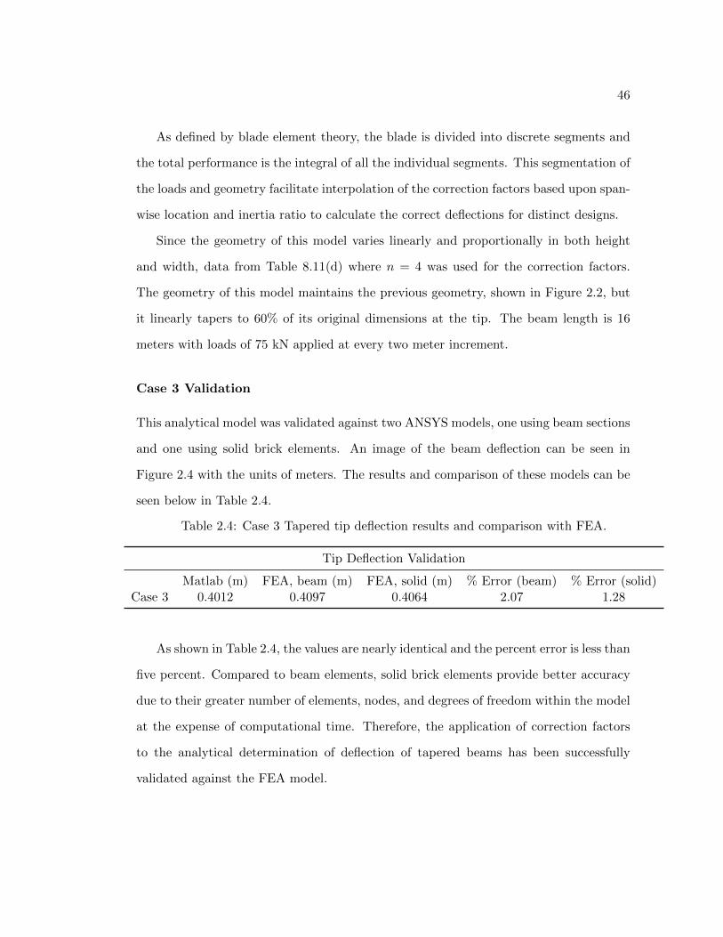
46

As defined by blade element theory, the blade is divided into discrete segments and

the total performance is the integral of all the individual segments. This segmentation of

the loads and geometry facilitate interpolation of the correction factors based upon span-

wise location and inertia ratio to calculate the correct deflections for distinct designs.

Since the geometry of this model varies linearly and proportionally in both height

and width, data from Table 8.11(d) where n = 4 was used for the correction factors.

The geometry of this model maintains the previous geometry, shown in Figure 2.2, but

it linearly tapers to 60% of its original dimensions at the tip. The beam length is 16

meters with loads of 75 kN applied at every two meter increment.

Case 3 Validation

This analytical model was validated against two ANSYS models, one using beam sections

and one using solid brick elements. An image of the beam deflection can be seen in

Figure 2.4 with the units of meters. The results and comparison of these models can be

seen below in Table 2.4.

Table 2.4: Case 3 Tapered tip deflection results and comparison with FEA.

Tip Deflection Validation

Matlab (m) FEA, beam (m) FEA, solid (m) % Error (beam) % Error (solid)Case 3 0.4012 0.4097 0.4064 2.07 1.28

As shown in Table 2.4, the values are nearly identical and the percent error is less than

five percent. Compared to beam elements, solid brick elements provide better accuracy

due to their greater number of elements, nodes, and degrees of freedom within the model

at the expense of computational time. Therefore, the application of correction factors

to the analytical determination of deflection of tapered beams has been successfully

validated against the FEA model.

47

Figure 2.4: Case 3 Tapered beam deflection results.

2.2.4 Case 4: Twisted and Tapered Beam Deflection

Case 4 is a combination of the previous two cases to ensure the proper results from a

combined case analysis before moving to a full blade analysis. For this case, the scale

distributions for the x-coordinates were not identical to the y-coordinates, and were

chosen to match the chord and percent thickness scaling of a previously designed sample

turbine blade. The twist and scaling distributions can be seen below in Table 2.5.

Continuing from Case 3, the deflection correction factors for n = 4 were used. How-

ever, due to the combination of twist and taper, the moment of inertia ratios, Iratio, from

both principal axes were averaged together to calculate a correct ratio before initiating

the calculations to determine the correction factors.

The root cross-sectional area is identical to the prior cases, seen in Figure 2.2, and

the forces were maintained at 75 kN loaded at every two meters.

48

Table 2.5: Case 4 Twist and Scale Distributions.

Case 4 Twist and Scale Distributions

x/l x (m) Twist (degrees) X-Scale Y-Scale0.125 2 14.00 0.95 0.990.25 4 10.50 0.88 0.980.375 6 7.50 0.79 0.950.5 8 5.00 0.73 0.93

0.625 10 3.00 0.70 0.910.75 12 1.50 0.63 0.850.875 14 0.50 0.59 0.76

1 16 0.00 0.54 0.69

Case 4 Validation

Again, since both the width and the height of the section varies with the spanwise

location, the table for n = 4 was used from Young’s textbook. A solid model was created

in SolidWorks, a commercial computer-aided design, CAD, software, and then exported

as an IGES file to ANSYS. This FEA model was developed with 20,160 elements with

the same geometry and loadings as discussed previously. Figure 2.5 displays the beam

deflection for Case 4 with units of meters.

Since the percent error is 6.31% and is within the 10% limit, seen below in Table 2.6,

the combination of the twisted and tapered methods has been validated. While this

percent error is higher than previous validation cases, it can be attributed to the rather

coarse segmentation and loading of the beam. It is projected and confirmed in the

next section that further resolution of the beam’s loads and geometry will provide more

accurate results. This model is comprised of eight segments, the model in Case 5 contains

30 segments.

Table 2.6: Case 4 Twisted and tapered tip deflection results and comparison with FEA.

Tip Deflection Validation

Matlab (m) FEA (m) Percent ErrorCase 4 0.3001 0.3203 6.31

49

Figure 2.5: Case 4 Twisted and tapered beam deflection results.

2.2.5 Case 5: Full Blade Tip Deflection

The next logical step after validating the twisted and tapered method as correct, an

actual turbine blade can finally be examined. One of the limitations of HARP Opt, as

discussed previously, is that it does not output root geometry. Thus, in order to cal-

culate accurate values for the inertia ratio, a routine was developed to extrapolate the

root geometry from the provided geometry. To achieve this, a cubic spline extrapolation

method was created in Matlab to add the root values of chord, twist, and percent thick-

ness. While it is generally unwise to use extrapolation methods due to uncertainty of

the results, the entire blade geometry is used to provide the basis for extrapolation and

the distance from the first section to the root is very small.

50

Case 5 Validation

This final case was validated against a full-scale solid blade that was meshed and analyzed

by David Dreese at ARL Penn State. This blade was designed using the optimization

code HARP Opt; the blade geometry and loading were taken from the output file and

blade-element data file. The thrust forces were applied at the mid-chord point at each

of the thirty sections along the span of blade. Since this blade was developed as part of

a company-sponsored project, a full CFD analysis was performed on this design. The

pressure loads from the CFD results were compared against using the point loads from

the blade-element momentum theory results. A comparison of the two results can be

seen below in Table 2.7. Due to the minimum percent error between the two studies, it

has been confirmed that using section thrust forces applied at the mid-chord points is

an accurate method to determine tip deflection in a full turbine blade.

Table 2.7: Comparison of blade tip deflections due to CFD pressure loads and BEMT point loads.

CFD Pressure Load (m) BEMT Point Loads (m) Percent Error

Blade Deflection 0.383 0.397 3.66

Again, for this case, the table for n = 4 from Table 8.11(d) in Roark’s Formula for

Stress and Strain was used. This blade design is proprietary, so the geometry of the

blade structure and foils used will not be provided; however, an image of the deflection

can be seen in Figure 2.6. This blade is approximately 20 meters in length, and the

deflections are shown at five times their displacement to show their behavior.

This full MHK turbine model contained a mesh of 31,000 elements with a combined

109,000 degrees of freedom. It used quasi-isotropic material properties that were reduced

to account for the environmental impacts on the material properties. This resulted in

approximately a ten percent decrease in the modulus of elasticity.

The results of this validation can be seen in Table 2.8. The percent error between

the predicted and calculated values is minimal. Continuing from the previous section’s

conclusion, this minimal error can be attested to the high resolution of the loads and

51

Figure 2.6: Case 5: Full Blade tip deflection results.

Table 2.8: Case 5 deflection results.

Tip Deflection Validation

Matlab (m) FEA (m) Percent ErrorCase 5 0.4025 0.397 1.39

geometry along the blade. Between Case #4 and Case #5, there is an increase from 8 to

30 segments, approximately a four times increase in the resolution of the blade geometry

and loads. The Matlab code used for this analysis has been included in Appendix A.

2.3 Torsional Deflection

A torsional deflection model was developed to study the impact of the sectional pitching

moment on the overall blade twist distribution. The pitching moment of a foil is a prop-

erty of the individual section, and this moment acts at the aerodynamic or hydrodynamic

center. The aerodynamic or hydrodynamic center is defined as the point at which the

52

Figure 2.7: Foil depicting pitching moment at quarter chord location [66].

pitching moment coefficient, CM , does not vary with angle of attack. For most foils,

the aerodynamic or hydrodynamic center is approximated to be located at the quarter

chord point, as seen in Figure 2.7, resulting in small variations in the moment coefficient

with angle of attack [66]. The pitching moment for a symmetric foil is zero. For modern

cambered foils, the pitching moment acts in the negative direction. This moment acts

to further twist the blade section and decrease the angle of attack.

To determine the pitching moment, the foil moment coefficient is needed. The pitch-

ing moment, Mtor, is a function of the dynamic pressure, planform area S, chord, and

the foil pitching moment coefficient moment in the form

Mtor =1

2ρV 2

relCMSC , (2.10)

where

Vrel =√

(Ωx)2 + V 2∞ . (2.11)

Since the pitching moment varies primarily as a function of the local velocity at

the section, the torsional behavior at each operational flow speed must be analyzed.

Additionally, the contribution of the outboard moments influence all the inner sectional

moments. Thus, a summation, shown in Equation 2.12, must be performed to take into

53

account the total torsional moment felt at each section:

Mlocal = Mtor +∑

Mtor,outboard . (2.12)

Once this summation has been completed, the spanwise local moment values are used

in the torsional deflection equation, where G is the modulus of rigidity, and J is the polar

moment of inertia, in the form

φind =Mlocal x

GJ. (2.13)

Equation 2.13 finds the local torsional deflection at each section. To determine the

global response, a summation of the local torsional deflections must be performed such

that

φlocal = φind +∑

φind,inboard . (2.14)

2.3.1 Torsional Deflection Validation

The torsional deflection validation was completed using two different models. One was

a cylindrical shaft that was analyzed using two different load cases. The second model

used a twisted rectangular beam with only one load case.

Cylindrical Shaft

The first step of the torsional deflection validation was completed using a solid cylindrical

shaft. This model was analyzed in two steps: loading at the tip, and then loading at

incremental sections along its length. This model was used since it is the simplest and

most used example for torsional deflection.

Both models contain the same geometry. The diameter is one meter with a total

length of ten meters. For both models, the torque was divided into 24 equal loads that

were applied at the perimeter nodes in the tangential direction. The results for the first

54

model can be seen in Table 2.9.

Table 2.9: Tip loaded shaft torsional deflection comparison.

Tip Loaded

x (m) Abaqus (deg) Matlab Code (deg) Percent Error0.5 0.138 0.138 2.261 0.275 0.269 2.25

1.5 0.413 0.407 2.252 0.550 0.539 2.25

2.5 0.693 0.676 2.253 0.831 0.808 2.25

3.5 0.968 0.945 2.244 1.106 1.077 2.24

4.5 1.243 1.215 2.245 1.381 1.352 2.24

5.5 1.518 1.484 2.246 1.656 1.621 2.24

6.5 1.793 1.753 2.237 1.931 1.891 2.23

7.5 2.074 2.023 2.278 2.240 2.160 3.48

Due to the consistency of the percent error along the length of the shaft, this method

is validated as correct. The variation at the tip is a result of how the loads are applied.

Since the torque is applied as discrete point loads on the nodes located on the perimeter

of the tip rather than a uniform moment over the entire cross section, there is an increase

in localized deflections at the nodes where the loads are applied. These local deflections

impact the global deflections at each location along the shaft, and thus cause a consistent

percent error along the length.

Once this simple model was analyzed and its discrepancies understood, a more com-

plex model was analyzed using multiple loads along the length of the shaft. For the

second model, the same loads were maintained, but they were also applied at each one

meter increment along the shaft.

The results of this analysis can be seen in Table 2.10. The percent error at the root

is more prominent due to the summation of forces along the beam length creating more

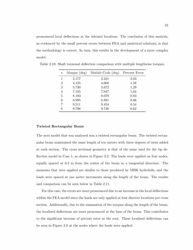
55

pronounced local deflections at the inboard locations. The conclusion of this analysis,

as evidenced by the small percent errors between FEA and analytical solutions, is that

the methodology is correct. In turn, this results in the development of a more complex

model.

Table 2.10: Shaft torsional deflection comparison with multiple lengthwise torques.

x Abaqus (deg) Matlab Code (deg) Percent Error

1 2.177 2.221 2.032 4.125 4.068 1.583 5.730 5.672 1.294 7.105 7.047 1.045 8.193 8.079 0.836 8.995 8.881 0.667 9.511 9.454 0.548 9.798 9.740 0.62

Twisted Rectangular Beam

The next model that was analyzed was a twisted rectangular beam. The twisted rectan-

gular beam maintained the same length of ten meters with three degrees of twist added

at each section. The cross sectional geometry is that of the same used for the tip de-

flection model in Case 1, as shown in Figure 2.2. The loads were applied on four nodes,

equally spaced at 0.5 m from the center of the beam in a tangential direction. The

moments that were applied are similar to those produced by MHK hydrofoils, and the

loads were spaced at one meter increments along the length of the beam. The results

and comparison can be seen below in Table 2.11.

For this case, the errors are more pronounced due to an increase in the local deflections

within the FEA model since the loads are only applied at four discrete locations per cross

section. Additionally, due to the summation of the torques along the length of the beam,

the localized deflections are more pronounced at the base of the beam. This contributes

to the significant increase of percent error at the root. These localized deflections can

be seen in Figure 2.8 at the nodes where the loads were applied.

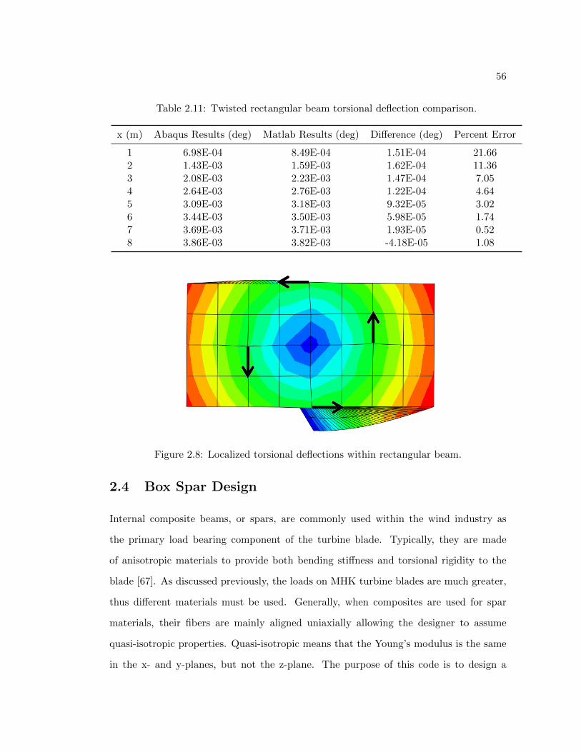
56

Table 2.11: Twisted rectangular beam torsional deflection comparison.

x (m) Abaqus Results (deg) Matlab Results (deg) Difference (deg) Percent Error

1 6.98E-04 8.49E-04 1.51E-04 21.662 1.43E-03 1.59E-03 1.62E-04 11.363 2.08E-03 2.23E-03 1.47E-04 7.054 2.64E-03 2.76E-03 1.22E-04 4.645 3.09E-03 3.18E-03 9.32E-05 3.026 3.44E-03 3.50E-03 5.98E-05 1.747 3.69E-03 3.71E-03 1.93E-05 0.528 3.86E-03 3.82E-03 -4.18E-05 1.08

Figure 2.8: Localized torsional deflections within rectangular beam.

2.4 Box Spar Design

Internal composite beams, or spars, are commonly used within the wind industry as

the primary load bearing component of the turbine blade. Typically, they are made

of anisotropic materials to provide both bending stiffness and torsional rigidity to the

blade [67]. As discussed previously, the loads on MHK turbine blades are much greater,

thus different materials must be used. Generally, when composites are used for spar

materials, their fibers are mainly aligned uniaxially allowing the designer to assume

quasi-isotropic properties. Quasi-isotropic means that the Young’s modulus is the same

in the x- and y-planes, but not the z-plane. The purpose of this code is to design a

57

quasi-isotropic or isotropic box beam within the blade that is capable of supporting the

peak bending moments that the turbine blade experiences. In this section, the term

shear web refers to the vertical sections of the box beam, and the term spar cap refers

to the upper and lower sections as shown in Figure 2.9.

Figure 2.9: Box beam section descriptions.

For this design, the main limiting factor is either the yield strength of the material,

σy, or the maximum allowable strain, εmax, where

σy = EεmaxSFstruct . (2.15)

Once the blade geometry, material properties, and flow properties are input, the code

initiates by defining the starting shear web locations of 20% and 50% chord. The code

then determines the upper and lower points on the foil at both chord locations within a

preset tolerance level. Next, the minimum height is chosen from each of the two shear

webs for the box beam height, such that the box beam fits within the foil shape. The

height is further reduced by taking into account the skin thickness of the turbine blade

at that spanwise location.

Sizing of the box beam wall thickness is completed by determining the moment of

inertia needed to resist the applied bending moments, while not exceeding the yield

58

strength of the material. The bending moment used for this case is the moment that is

normal, MN , to the chord. This is done in a two-step process by first determining the

required moment of inertia and then determining the necessary wall thickness to match

this value. To determine the required moment of inertia value, Ilocal, the equation for

bending stress is used where

σy =MNy

Ilocal. (2.16)

Rearranging this equation results in

Ilocal =MNy

σy. (2.17)

Figure 2.10: Box beam model dimensions.

For a box beam, as displayed in Figure 2.10, the second moment of inertia equation

takes the form

Ilocal =BoH

3o

12− BiH

3i

12, (2.18)

where

59

Bi = Bo − 2t (2.19)

and

Hi = Ho − 2t . (2.20)

Rearranging the equations and solving for the wall thickness, t, is unnecessary in this

case. Instead, a function iteration method is quickly used to determine the correct wall

thickness. This approach is possible because the desired value of Ilocal is known and a

comparison to this value can quickly be made. This approach defines t = 0, and then

iterates by increasing the wall thickness by 0.1 mm during each step. A comparison of

the desired moment of inertia ratio to the calculated value is made, and the method

is complete when these values are equal. The routine breaks and iterates to the next

sections if the wall thickness is greater than half the width of either the base or the

height.

The final piece of this code is to minimize the volume, and subsequently cost, of

the box beam by comparing different shear web locations. As the web location moves

towards the leading or trailing edges, the dimensions of the box beam change in order to

resist the bending moments. Once the code determines the minimum weight, the final

box beam dimensions and shear web locations are provided in the final output structure.

2.5 Stress Model Validation

A more complex model of the blade structure is currently being developed and validated

for use in a future release of HARP Opt. This model allows for more accurate structural

design and optimization by using three materials for the spar caps, shear webs, and blade

skin to form a composite blade structure.

The process for solving for the stresses involves using weighted values for the material

60

properties based on their individual impact to the total material behavior. This method

is described in Bauchau’s book ”Structural Analysis with Applications to Aerospace

Structures.” [68]. It involves using weighted sums of the sectional properties such as

area, centroid location, and moments of inertia, in order to create modulus weighted

properties. These weighted properties, as indicated by the terms with the ∗, are then

used in Equation 2.21 to calculate the stress at that point:

σ =E

Eref

[F

A∗− MyI

∗x +MxIxy

∗

I∗xI∗y − I∗2xy

x+MxI

∗y +MyIxy

∗

I∗xI∗y − I∗2xy

y

]. (2.21)

This model validation is part of an ongoing effort with Danny Sale to validate this

stress model before the next release of HARP Opt. Mr. Sale has developed the routines

and subroutines to calculate the stress, and the object of this work was to develop a

similar finite element model to validate the stress values.

Figure 2.11: Stress model beam dimensions and loadings.

The ANSYS model was developed using two different materials for the shear webs

and spar caps. The spar caps were composed of a material with Ecap = 41.8 GPa, and

the shear webs were a more flexible material with Eweb = 13.3 GPa. In order to minimize

localized deflections, a uniform pressure of 100, 000 Pa was applied to the surfaces. The

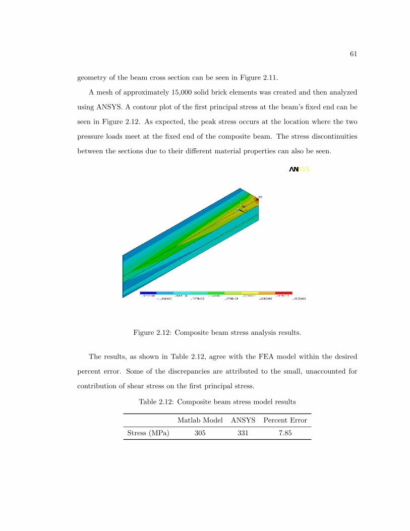
61

geometry of the beam cross section can be seen in Figure 2.11.

A mesh of approximately 15,000 solid brick elements was created and then analyzed

using ANSYS. A contour plot of the first principal stress at the beam’s fixed end can be

seen in Figure 2.12. As expected, the peak stress occurs at the location where the two

pressure loads meet at the fixed end of the composite beam. The stress discontinuities

between the sections due to their different material properties can also be seen.

Figure 2.12: Composite beam stress analysis results.

The results, as shown in Table 2.12, agree with the FEA model within the desired

percent error. Some of the discrepancies are attributed to the small, unaccounted for

contribution of shear stress on the first principal stress.

Table 2.12: Composite beam stress model results

Matlab Model ANSYS Percent Error

Stress (MPa) 305 331 7.85

62

2.6 Tip Vortex Cavitation

The final enhancement model that was created for inclusion into HARP Opt was a tip

vortex cavitation prediction model. Development of this model was requested by Danny

Sale as part of an interview about desired additions to the optimization code [65]. While

this type of cavitation does not directly impact the blade performance, understanding

its inception is important because of the potential impact to downstream structures and

operational noise. As such, the outputs for this routine do not affect the optimization

process. As discussed previously in Chapter 1, the tip vortex cavitation number is defined

as

σi = KC2LRe

m . (2.22)

For tip vortex cavitation to occur, σi > −Cp,vortex. For this routine, to find the CL,

the average of the outer 20% of the blade span was used. The tip Reynolds number was

used for the Re term. Also, since this is a generic equation that must predict results for

a wide array of foils and designs, the coefficient K was set to equal 0.54, which is the

average of experimentally derived values of this coefficient [44]. As discussed in Chapter

1, the value for m is commonly accepted to be 0.4 [44]. This subroutine provides the

tip vortex cavitation free depth, where W is equal to the blade tip velocity, for each

operational flow speed of the turbine as defined by:

hvortexfree =σi

12ρW

2 − Patm + Pvap

ρg. (2.23)

63

2.7 Enhancements Summary

These structural and cavitation enhancements to HARP Opt were written to improve

the usefulness of the results. The tip deflection model ensures that the blade tip will

not impact downstream structures, such as a tower, during normal operation. Also, the

torsional deflection model allows the design to consider the effects of angular deflection

based upon the operating conditions. It is important to note, that the tip deflection does

not affect the power output of the turbine, as it does not change the twist angle of the

blade. Conversely, the torsional deflection of the blade does have the potential to reduce

the turbine power output since it directly impacts the twist angle, and thus angle of

attack, of the blade sections. The box beam design code completes a coarse spar design

that can be further improved using post-processing tools. The last of the structural

design enhancements validated a new composite box beam design code written by Danny

Sale. As initially desired, each of these structural improvements were validated to within

10 percent error, with some within 5 percent. The last model is a coarse assessment of

tip vortex cavitation to better understand the tip vortex cavitation-free depth of the

turbine blade.

The next chapter focuses on application of these design tools on a reference marine

hydrokinetic turbine design. After a turbine design has been performed, these tools will

be used to ensure proper operational behavior.

Chapter 3Reference Marine Hydrokinetic

Turbine Design

To initiate a turbine blade design, many design parameters must be determined and

defined. The resource, turbine geometry, blade material, foil shapes, and drivetrain

configuration must all be considered and defined before the blade design can be initiated.

Once these properties are set, a parametric study can be performed to compare various

designs with differing number of blades and power configurations. Lastly, the structural

design enhancements are applied to the final design to study their effects.

3.1 Resource Assessment

Since the overall goal of energy capture is for economic gain, the logical place to begin

when initiating the design of a marine hydrokinetic turbine is to decide the site location.

This is critical because the site must be able to produce the desired turbine power output

to make the design cost effective. In this design, the desired turbine power output is

in the range of 500-1000 kW, thus the location must be capable of generating sufficient

power. Additionally, the depths of the location must be suitable as to not impact marine

traffic while facilitating energy capture. In an actual deployment of marine hydrokinetic

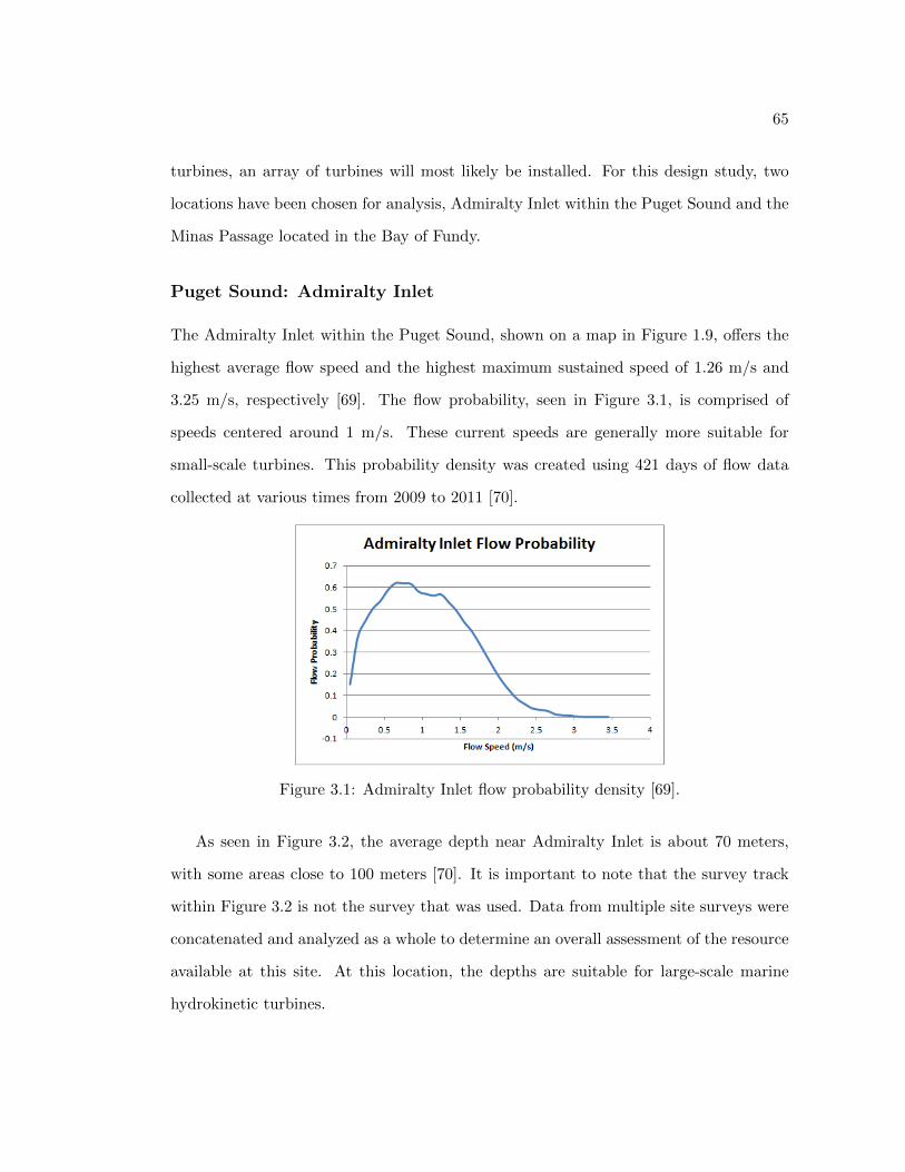
65

turbines, an array of turbines will most likely be installed. For this design study, two

locations have been chosen for analysis, Admiralty Inlet within the Puget Sound and the

Minas Passage located in the Bay of Fundy.

Puget Sound: Admiralty Inlet

The Admiralty Inlet within the Puget Sound, shown on a map in Figure 1.9, offers the

highest average flow speed and the highest maximum sustained speed of 1.26 m/s and

3.25 m/s, respectively [69]. The flow probability, seen in Figure 3.1, is comprised of

speeds centered around 1 m/s. These current speeds are generally more suitable for

small-scale turbines. This probability density was created using 421 days of flow data

collected at various times from 2009 to 2011 [70].

Figure 3.1: Admiralty Inlet flow probability density [69].

As seen in Figure 3.2, the average depth near Admiralty Inlet is about 70 meters,

with some areas close to 100 meters [70]. It is important to note that the survey track

within Figure 3.2 is not the survey that was used. Data from multiple site surveys were

concatenated and analyzed as a whole to determine an overall assessment of the resource

available at this site. At this location, the depths are suitable for large-scale marine

hydrokinetic turbines.

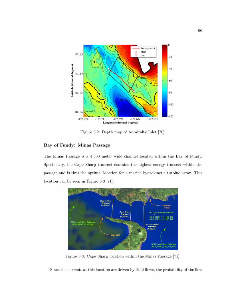
66

Figure 3.2: Depth map of Admiralty Inlet [70].

Bay of Fundy: Minas Passage

The Minas Passage is a 4,500 meter wide channel located within the Bay of Fundy.

Specifically, the Cape Sharp transect contains the highest energy transect within the

passage and is thus the optimal location for a marine hydrokinetic turbine array. This

location can be seen in Figure 3.3 [71].

Figure 3.3: Cape Sharp location within the Minas Passage [71].

Since the currents at this location are driven by tidal flows, the probability of the flow

67

is skewed to below 2.0 m/s. The current probability density can be seen in Figure 3.4 [71].

From this density function, the time-averaged flow speed for this site is 1.68 m/s.

Figure 3.4: Flow probability density of the Cape Sharp tidal resource [71].

Additionally, the depths at this area, as shown in Figure 3.5, are very capable of

supporting large-scale marine hydrokinetic turbines [71]. There is also sufficient depth

to allow for navigational clearance of ships.

Figure 3.5: Depth profile of Cape Sharp [71].

3.1.1 Resource Selection

After careful analysis of the current speeds, Admiralty Inlet within the Puget Sound in

Washington was chosen to be the desired resource for this marine hydrokinetic reference

design. This area features a tight range of average current speeds. The Minas Passage

features as reasonable average current speed of 1.68 m/s, but experiences currents up to

68

4.9 m/s. These high flow speeds pose a significant design challenge to control the power

generation at these high flow speeds, to control surface cavitation, and to maintain

structural integrity of the blade. As a result, Admiralty Inlet is more desirable due to

its tight distribution of flow speeds that are less than 2.0 m/s.

3.2 Foils Considered

For this design study, four families of foils were studied: NREL, FFA, Delft, and Althaus.

Foils from all of these families have been used with wind turbine blade designs. Three

foils from each family, corresponding to the root, mid, and tip sections of the turbine

blade, were examined. When analyzing and comparing the foils against each other, the

Reynolds number plays an important role in foil properties. The Reynolds number will

vary due to the change in local velocity along the blade span and the change in chord

lengths along the blade span. Based on anticipated turbine sizing, the Reynolds number

will likely vary between 1 and 10 million, but the average will remain around 5 million.

However, in order to facilitate foil selection, a constant Reynolds number of 5 million

was used to allow for comparison of foils across many families.

To calculate the foil properties, XFOIL, a panel method boundary layer solver, was

used to determine the foil properties at varying angles of attack [72]. This analysis

was performed with an Ncrit equal to 5 due to the turbulent inflow conditions found in

marine environments. This Ncrit value corresponds to the n term within the en method

for prediction of transition within laminar boundary layers. XFOIL utilizes a simplified

envelope version of the en method that produces minimal error as compared to the full

en method. Higher Ncrit values correspond to low levels of ambient disturbance, whereas

low values correspond to high levels of ambient disturbance [73].

69

3.2.1 NREL

The NREL foils that are being examined are the S818, S816, and S817 for the root,

mid, and tip foils, respectively, as shown in Figure 3.6. These foils are a family of thick

laminar-flow foils that were designed for 30 to 40 meter horizontal-axis wind turbines.

Their design objectives were restrained maximum lift, insensitive to roughness, and

low profile drag [74]. The NREL foils are also relatively thick foils along the entire

chord length of the section. This is desirable for structural integrity of the blade during

operation. These foils feature a very high lift-to-drag ratio at rather low angles of attack.

(a) S818 Root Foil. (b) S816 Mid Foil. (c) S817 Tip Foil.

Figure 3.6: NREL Family Foils [74].

3.2.2 FFA

The FFA foils were developed by the Aeronautical Research Institute of Sweden. Shown

in Figure 3.7, the three FFA foils are that were considered were the FFA W3-301, FFAW

3-241, and FFA W3-211 for the root, mid, and tip sections, respectively. The W3-

301 is one of the most common root shapes for wind turbines [75]. Both the W3-241

and W3-301 foils have been used on inboard sections of various Danish wind turbine

blades [76]. The W3-211 is a thinner section that is typically used for tip sections. All

foils feature a smooth stall transition with a nearly identical CL,max. However, their

maximum lift-to-drag ratio peaks at rather high angles of attack as compared to the

other foils. Consequently, their pressure coefficients are the lowest among the foils that

were studied.

70

(a) W3-301 Root Foil. (b) W3-241 Mid Foil. (c) W3-211 Tip Foil.

Figure 3.7: FFA Family Foils [64].

3.2.3 Delft

The Delft University foils are currently in use by manufacturers in over ten wind turbine

blades with diameters from 29 to over 100 meters [77]. The Delft 97-W-300 foil is a

thick root foil with a high CL,max that was designed primarily for structural reasons.

The DU91-W2-250 and DU93-W-210 foils are mid and tip foils, respectively, and were

designed with CL,max of about 1.5, a smooth stall, and insensitivity to leading edge

roughness [76]. The tip foil, DU93-W-210, was also designed to minimize aerodynamic

noise [78]. These foils can be seen in Figure 3.8.

(a) DU97-W-300 Root Foil. (b) DU91-W2-250 Mid Foil. (c) DU93-W-210 Tip Foil.

Figure 3.8: Delft Family Foils [64].

3.2.4 Althaus

The Althaus foils, shown in Figure 3.9, were designed by D. Althaus from the Institute

for Aerodynamics and Gasdynamics of the University of Stuttgart, Germany [79]. These

foils feature high CL,max and CLCDmax

values with fairly low pressure coefficients. They

all feature a benign stall region with nearly uniform CL values post-stall.

71

(a) AH93-W-300 Root Foil. (b) AH93-W-257 Mid Foil. (c) AH93-W-215 Tip Foil.

Figure 3.9: Althaus Family Foils [80].

3.2.5 Foil Selection

Table 3.1: Comparison of foil properties

Family Foil % Thickness CL,maxCLCDmax

α at CLCDmax

Cp,min atCLCDmax

NREL S818 24 1.7 140 5 -1.75NREL S816 21 1.5 132 3.5 -1.15NREL S817 16 1.45 162 2.5 -0.96FFA W3-301 30 1.7 125 9.5 -4.6FFA W3-241 24 1.66 132 7.5 -2.22FFA W3-211 21 1.69 147 6 -1.78

Althaus AH93-W-300 30 1.75 105 7 -2.66Althaus AH93-W-257 25 1.65 140 5.5 -1.73Althaus AH93-W-215 21 1.52 128 6.5 -1.7

Delft DU97-W-300 30 1.76 124 7.5 -2.28Delft DU91-W2-250 25 1.74 141 4.5 -1.58Delft DU93-W-210 21 1.83 148 3.5 -1.36

A full comparison of the foil properties are listed in Table 3.1. After careful consid-

eration, the final foils that were chosen were the DU91-W2-250, NREL S816, and NREL

S817 for numerous reasons. As discussed previously in Chapter 1, the root foil’s primary

function is for structural stability with a high CL,max. The DU91-W2-250 meets these

requirements; however, it does have a rather high pressure coefficient as compared to the

NREL foils.

The mid-span foil was selected to be the NREL S816. This foil has a high CLCDmax

value combined with low pressure coefficient value to mitigate surface cavitation. Unlike

most foils where there is a spike in the pressure coefficient near the leading edge, the

72

NREL S816 features a very low minimum pressure coefficient that peaks at the mid-

chord location. A graph of the pressure coefficient versus chord location can be seen in

Figure 3.10.

The tip foil was chosen to be the NREL S817 foil. This foil features many desirable

properties for a tip foil. The S817 foil has the highest CLCDmax

of all the foils that were

examined, and it is able to achieve this because it is the thinnest foil that was studied.

This foil also features an exceptionally low pressure coefficient at its maximum lift-to-

drag ratio, seen in Figure 3.10, that does not reach its maximum until approximately

the mid-chord location.

Figure 3.10: Cp versus xC of S816 foil at α = 2.5

3.3 Drivetrain Configuration

Due to the increase in maintenance costs for marine hydrokinetic turbines and potential

environmental impacts, the drivetrain configuration must be selected wisely to allow for

prolonged, uninterrupted operation. This turbine will utilize a fixed-pitch blade system

to eliminate the need for pitch motors. Power generation will be controlled through

torque limiting within the generator through back EMF, electromotive force, control

73

and with passive stall of the blades. Additionally, it will operate in a variable speed

operation, thus allowing the design to optimize to the maximum power coefficient for

each flow speed. It is anticipated that the RPM of the turbine will optimize to between

5-8 RPM, which is quite low as compared to wind turbines in Table 1.1. As a result,

a gearbox will need to be used to step up the rotational velocity that a variable-speed,

asynchronous generator needs to operate.

Also, since tidal areas experience the reversal of flow direction twice a day, the turbine

needs to orient itself to capture energy in both directions. This can be accomplished

either by yawing the entire turbine 180 degrees, or by pitching each blade 180 degrees.

For simplicity, this design will utilize a passive yaw system to align the turbine in the

flow direction.

3.4 Initial Geometry

Table 3.2 provides the optimization control point locations and bounds at each spanwise

location selected to facilitate the design optimization process within HARP Opt. The

optimization bounds for the chord and twist were selected to be large, but the foil

locations were much more constrained. They were defined to be the Delft DU91-W2-

250 at the root, the NREL S816 at 70 to 80% span, and the NREL S817 at the tip.

Fluid properties for sea water at 10C were used as inputs into HARP Opt. For the

structural optimization process, an E-glass/epoxy composite with a Young’s modulus of

20 GPa was used with a maximum strain of 2500 micro-strain. The flow probability

density function at Admiralty Inlet was used to drive the AEP optimization. Once all

these parameters were defined, a parametric design was performed to analyze turbines

of different configurations and rated power.

74

Table 3.2: Optimization control point locations and bounds

x/r Twist LB (deg) Twist UB (deg) Chord LB (m) Chord UB (m)

0.17 0 40 3 50.24 0 40 2.5 4.50.41 0 40 2 40.68 -10 40 1.5 3.51.00 -10 40 1 3

3.5 Parametric Study

A parametric study, as outlined in Table 3.3, was developed to examine various blade

designs based on desired power output, blade number, hub diameter, and rotor diameter.

A total of six cases were examined and compared against each other. Three different

cases of rated power each with two and three bladed configurations were examined. The

hub diameters were determined based on the required circumference needed to attach the

desired number of blades with the maximum root chord of 5 meters. The rotor diameters

were selected using the power equation, Equation 1.20, with an assumed power coefficient

of 0.45 and a rated flow speed of 1.5 m/s.

Table 3.3: Table of turbine parametric design.

Case # # Blades Rated Power (kW) Rotor Diameter (m) Hub Diameter (m)

1 2 1000 28.5 3.52 3 1000 28.5 53 2 750 24.5 3.54 3 750 24.5 55 2 500 20 3.56 3 500 20 5

A surface cavitation assessment was performed for estimated rotor speeds, rotor

diameters, and chord values at the root, mid, and tip sections. Substituting in the tip

speed, W , for Uinfty in Equation 1.29, the cavitation numbers at the root, mid, and tip

locations and all flow speeds were determined. With The lowest cavitation number was

determined to be 6, which occurs at the blade tip at an inflow speed of 1.4 m/s. The

75

Cpmin value of the tip foil at this condition is -0.826. As a result of the assessment, as

indicated by Equation 1.31, this turbine will not experience surface cavitation at any

flow speed since the cavitation numbers are much higher than the −Cpmin values.

A summary of the results of the parametric design can be seen in Tables 3.4 and 3.5.

All of the turbine designs behaved as desired; all reached their rated power at the desired

flow speed of 1.5 m/s. Also, all the designs had nearly identical power coefficients and

capacity factors of 0.47 to 0.48 and 43% to 44%, respectively. The two-bladed designs also

optimized to designs that had rotor torques of approximately 80% of their three-bladed

counterparts. The two bladed designs therefore optimized to higher rotational speeds to

achieve the same power output with higher tip speed ratios. The thrust forces varied

slightly, but they were within approximately 10% of each other. For all the turbines,

root chords and tip chords were all large. But, as a product of the optimization process,

there was a variance within the taper ratio, which is the ratio of the hub-to-tip chords.

For the 1000 kW and 750 kW design cases, the taper ratio was approximately 0.5 for

two-bladed designs, and 0.3-0.4 for three-bladed designs. However, for the 2-bladed 500

kW design case, the taper ratio is almost half of the other 2-bladed designs. This can be

attributed to the increased rotor RPM and reduced rotor torque and loads the blades

experience, which allows the blades to structural optimize to slimmer profiles.

Table 3.4: Comparison of power results from parametric design.

Case # CP @ Prated AEP (kW-hr/yr) CF (%) RPM @ Prated TSR @ Prated

1 0.473 3775573 43.1 4.58 6.392 0.474 3841202 43.8 3.76 5.253 0.474 2857624 43.5 4.67 5.714 0.487 2898298 44.1 4.43 5.415 0.476 1936902 44.2 6.18 6.266 0.480 1944847 44.4 5.12 5.18

76

Table 3.5: Comparison of load and chord results from parametric design.

Case # Thrust (kN) Torque (kN-m) Root Chord (m) Tip Chord (m) Taper Ratio

1 1167 2088 4.386 2.279 0.5202 1068 2547 4.539 1.225 0.2703 717 1536 3.605 1.942 0.5394 809 1928 3.900 1.508 0.3875 535 913.1 4.373 1.243 0.2846 536 1196 3.989 1.266 0.317

3.6 Final Design

The selected design is the two bladed 500 kW turbine, shown as Case #5 in Tables 3.3

to 3.5. As seen in Figure 3.11a, this turbine reaches rated power at the desired flow

speed of 1.5 m/s. However, this is a forced power control by decreasing the RPM

after rated power has been reached. The torque produced by the turbine still increases,

but the rotor speed is reduced to maintain nearly constant power. This turbine was

selected because it has the second highest capacity factor, the highest rotor rpm at rated

speed, the second highest tip speed ratio, the lowest rotor torque, and the lowest rotor

thrust. The difference between the two- and three-bladed designs were minimal in power

production, but the cost of a third blade adds 50% to the total cost of materials for the

blades. The high tip speed ratio, as shown previously in Figures 1.15 and 1.16, results in a

minimum drop in the power coefficient when operating with only two blades as compared

to its three-bladed counterpart. The lower torque and thrust values are also desirable to

develop a robust gearbox and drive train. This turbine has an estimated annual energy

production of approximately 1.9 million kW-hr/year with a capacity factor of 44.2 that

is superior to both onshore and offshore wind as shown previously in Table 1.3.

Additionally, at the rated flow speed, the lift coefficient is high at the root, 1.23, and

then tapers, almost linearly, to 0.50 at the tip. The blade maintains a nearly uniform

CLCD

of 100 for the entire blade span, increasing slightly at the blade tip. Also, as shown

through the torque and thrust graph in Figure 3.11b, the blade loadings peak at about

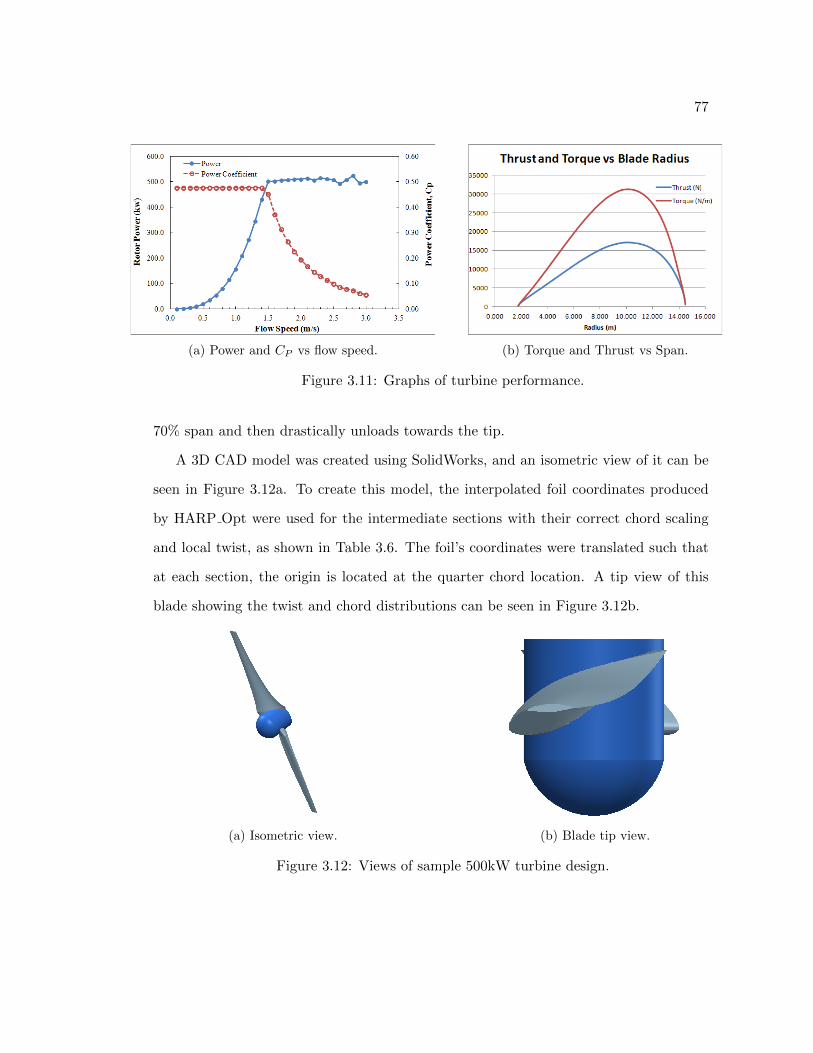
77

(a) Power and CP vs flow speed. (b) Torque and Thrust vs Span.

Figure 3.11: Graphs of turbine performance.

70% span and then drastically unloads towards the tip.

A 3D CAD model was created using SolidWorks, and an isometric view of it can be

seen in Figure 3.12a. To create this model, the interpolated foil coordinates produced

by HARP Opt were used for the intermediate sections with their correct chord scaling

and local twist, as shown in Table 3.6. The foil’s coordinates were translated such that

at each section, the origin is located at the quarter chord location. A tip view of this

blade showing the twist and chord distributions can be seen in Figure 3.12b.

(a) Isometric view. (b) Blade tip view.

Figure 3.12: Views of sample 500kW turbine design.

78

Table 3.6: Geometry distribution for sample 500kW turbine design.

x/r Radius (m) Pre-Twist (deg) Chord (m) % Thick

0.122 1.767 26.43 4.373 24.40.127 1.837 25.91 4.298 24.30.136 1.976 24.93 4.166 24.30.150 2.182 23.60 4.001 24.20.169 2.453 22.05 3.822 24.10.192 2.786 20.36 3.639 24.00.219 3.177 18.61 3.458 23.90.250 3.623 16.84 3.279 23.70.284 4.119 15.14 3.108 23.50.321 4.658 13.51 2.941 23.30.361 5.235 12.02 2.783 23.10.403 5.844 10.65 2.630 22.90.447 6.477 9.43 2.485 22.70.492 7.129 8.36 2.348 22.40.537 7.792 7.43 2.217 22.20.583 8.458 6.64 2.094 22.00.629 9.121 5.97 1.979 21.70.674 9.773 5.41 1.872 21.50.718 10.406 4.94 1.773 21.20.760 11.015 4.54 1.683 21.00.799 11.592 4.20 1.601 20.30.837 12.131 3.91 1.528 19.50.871 12.627 3.66 1.463 18.80.902 13.073 3.44 1.407 18.10.929 13.464 3.26 1.360 17.50.952 13.797 3.10 1.320 17.00.970 14.068 2.96 1.289 16.60.984 14.274 2.86 1.266 16.30.994 14.413 2.79 1.251 16.10.999 14.483 2.76 1.243 16.0

3.7 Application of Design Code Enhancements

3.7.1 Box Beam Design

The automated box beam spar design can be seen in Figure 3.13a with a sample cross

section shown in Figure 3.13b. Due to the large loads seen by this blade, the box spar

material is different than that chosen for the blade design optimization. For this design,

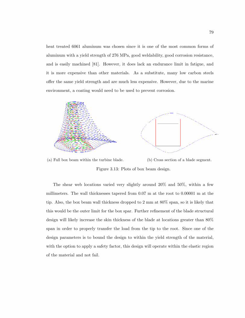
79

heat treated 6061 aluminum was chosen since it is one of the most common forms of

aluminum with a yield strength of 276 MPa, good weldability, good corrosion resistance,

and is easily machined [81]. However, it does lack an endurance limit in fatigue, and

it is more expensive than other materials. As a substitute, many low carbon steels

offer the same yield strength and are much less expensive. However, due to the marine

environment, a coating would need to be used to prevent corrosion.

(a) Full box beam within the turbine blade. (b) Cross section of a blade segment.

Figure 3.13: Plots of box beam design.

The shear web locations varied very slightly around 20% and 50%, within a few

millimeters. The wall thicknesses tapered from 0.07 m at the root to 0.00001 m at the

tip. Also, the box beam wall thickness dropped to 2 mm at 80% span, so it is likely that

this would be the outer limit for the box spar. Further refinement of the blade structural

design will likely increase the skin thickness of the blade at locations greater than 80%

span in order to properly transfer the load from the tip to the root. Since one of the

design parameters is to bound the design to within the yield strength of the material,

with the option to apply a safety factor, this design will operate within the elastic region

of the material and not fail.

80

3.7.2 Tip Deflection

Once the design process was complete, the tip deflection of the box beam model designed

previously was calculated using the methods described in Chapter 2. The loads used were

the thrust loads from the maximum case– which, in this design, is the rated flow speed.

There was no safety factor applied to the loads to determine the unbiased deflection.

The tip deflection for this design with the previously designed box beam is 0.278 m.

This value is reasonable and represents 1.9% of the total blade length. The deflections of

this blade is low due to the large width of the blade sections. This facilitates the design

of a box beam with a large moment of inertia, creating a stiff blade. Since this deflection

is very small, this turbine can be used in an upstream orientation without the potential

for tower strikes.

3.7.3 Torsional Deflection

A torsional deflection analysis, as discussed in Chapter 2, was performed on this box

beam design, and the results are very desirable. At each flow speed, there are minimal

angular deflections that affect the angle of attack at each section. As seen in Figure 3.14,

there is essentially no change in the power curve up to the rated flow speed. After the

turbine stalls, the power curve seems to diverge away from the original, undeflected

design. However, the foil pitching moment coefficients from XFOIL are not accurate for

post-stall conditions. Thus, a quantitative comparison of turbine power after stall cannot

be accurately performed for any turbine. This analysis validates the hydrodynamic

design of the turbine by ensuring that before stall the turbine power will not be negatively

affected by torsional deflections of the blade segments.

3.7.4 Tip Vortex Cavitation Analysis

As expected, tip vortex cavitation is a concern at nearly every flow speed. Shown in

Figure 3.15, at values where the curve is positive, tip vortex cavitation will occur. For all

flow speeds greater than 0.5 m/s, tip vortex cavitation will occur. This does not impact

81

Figure 3.14: Original and deflected power curves.

Figure 3.15: Vortex cavitation-free depth corrected for blade tip depth.

the hydrodynamic performance of the blade, but it can affect downstream structures and

impact the noise produced by the turbine.

82

3.8 Turbine Design Summary

To summarize this chapter, a full turbine blade was designed using HARP Opt. The

process began with a resource assessment and comparison of both the Admiralty Inlet

within the Puget Sound and Minas Passage within the Bay of Fundy. Once a resource

was selected, a study of foils was completed. Three foils were selected, one each for

the root, mid, and tip sections. Next, a parametric design study was performed to

compare six sample turbines of various size, configuration, and power output. The design

that was selected for the final design was a two-bladed, 500 kW, 29-meter diameter

turbine. Annually, each turbine will produce 1.9 million kW-hr per year, yielding a

turbine capacity factor of 44.2. Lastly, the analysis and design codes were applied to

this beam to determine the tip deflection, torsional deflection, and design a box beam

spar.

Chapter 4Summary and Conclusion

4.1 Summary of Work

In order for individual states within the United States to meet their renewable energy

goals, new sources of energy must be used for production. Within the marine environ-

ment, further development of conventional hydropower is limited due to the high capital

cost associated with construction and the limited resources that are still available. For

states that have tidal or current resources, marine hydrokinetic devices are the solution

to extract a cost-effective form of energy from that resource.

Previous marine hydrokinetic designs have utilized many of the lessons learned from

the wind turbine industry. In fact, many initiated their design process by essentially

trying to emulate the designs of wind turbine blades. However, as many companies

discovered, the sub-sea environment poses numerous challenges to structural design.

Primarily, due to the density difference between air and water, the loads that the turbine

blades experience are nearly three orders of magnitude higher. Thus, blades must be

carefully designed to be able to operate under these loading conditions. Additionally,

since maintenance operations on many MHK turbines is so costly, the drive and control

systems must be designed for simplicity and long-term life.

In order to facilitate the structural and hydrodynamic designs of these turbines, de-

84

sign and analysis tools were developed to be incorporated within HARP Opt, a NREL

horizontal-axis turbine design and optimization code. Where applicable, all the models

were validated to be within 10% error, preferably 5% error. Tip and torsional deflec-

tion models were created and validated using the commercial FEA solvers, ANSYS and

Abaqus. Tip deflection is vital to prevent interaction with downstream structures. When

the blade has enough resolution of loads and geometry along its span, this model was

validated to be within 2% error.

The torsional deflection of the blade during operation affects the local twist angles of

the blade. This in turn affects the angle of attack at that section and the lift and drag

forces produced. It is important, specifically when designing fixed-pitch blades, that the

power generated does not change due to operating characteristics of the blades. This

model was validated using shaft and beam FEA models. There were some discrepancies

between the analytic and FEA solutions; however, these errors were attributed to how

the loads were applied on the models themselves. These models were examined and

validated using solid beam structures. However, since these deflection models are driven

by the moment of inertias at each section, they can be applied to blades that utilize a

box beam or other spar structure.

As part of the final design process for HARP Opt an iterative box beam design code

was created to design a box beam that is within the yield strength or strain of the desired

material. The outer limit of the box beam’s dimensions are the shape of the foil. This

code works to minimize the weight, and thus cost, of the beam by iterating the shear

web locations to the optimal locations. Currently in development by Danny Sale at the

University of Washington is a composite box beam stress model. Analysis and validation

of his analytical approach was conducted using a composite box beam structure within

ANSYS. In its current form, this code was validated to within 10% error. However, this

model is being revised with the goal of being within a 5% error for the final version.

Lastly, a reference turbine design was developed to apply these models. The resource

selected was located at Admiralty Inlet within the Puget Sound in the state of Washing-

85

ton. Careful analysis and selection of foils were performed to achieve desirable operation

while mitigating cavitation on the blade surface. The foils that were selected were the

DU91-W2-250, NREL S816, and the NREL S817 for the root, mid, and tip foils, respec-

tively. A parametric design study was performed to compare the designs of turbines of

various configurations of both rated power and number of blades. The optimal design, a

two-bladed 20-meter diameter turbine that produces 500kW, was selected based on its

operating characteristics, tip-speed ratio, efficiency, and annual energy production val-

ues. A surface cavitation assessment was performed, assuming a smooth surface without

any roughness, to ensure that this form of cavitation will not occur and degrade rotor

performance.

For this design, the analysis and design methods, which were developed previously,

were applied to this model. A box beam design, comprised of 6061 heat treated aluminum

was designed for this blade shape. The shear web locations for this box beam were located

at approximately the 20% and 50% chord locations, with a wall thickness of 0.07 m at

the root tapering to 0 m at the tip. With further analysis, the blade skin could be

designed to eliminate the need for a spar at 80% span where the thickness drops to two

mm. This box beam was then analyzed for tip deflection and torsional deflection. The

tip deflection for this design is calculated to be 0.297 meters at the maximum thrust

condition, and the torsional deflection reduces the power by less than a kilowatt at flow

speeds prior to rated power. For this design, it was determined that tip vortex cavitation

will be a concern for all flow speeds greater than 0.5 m/s; however, this type of cavitation

does not affect blade performance.

These methods and understanding of their impact are very important to marine hy-

drokinetic turbine blade design. As compared to their wind counterparts, these turbines

experience much greater loads. As such, structural design and analysis of the blades is

imperative to proper operation of these blades.

86

4.2 Future Work

The design code HARP Opt is still in its infancy. Thus, as the code becomes more and

more complex and encompassing, there are many areas where it can improve. The first

step would be to improve the stress model to better match the FEA predictions. In

the past, a scientist at the National Renewable Energy Lab produced a composite spar

and blade design code called Gunjit. If possible, incorporation of that design code in the

optimization routine could prove valuable. Vibrations within the various turbine systems

can cause undesired effects within other parts, most notably the blades. Calculations

of the natural frequency and harmonics of the blades would prove beneficial to prevent

induced vibrations at those frequencies into the blades.

Appendix

Tip Deflection Code

function [Output] = Tip Deflection(RElm,TWIST,CHORD,PERCENT THICKNESS,AoA,AFang,...

LocVel,Cl,Cd,Thrust,I1,I2,Ixx,Iyy,Ixy)

global HubRad RotorRad NumCases rho NumSeg Einput MaxTipDefl MaxTipDefl;

for i=1:length(I1)

Iratio1(i,1) = I1(1)/I1(i);

end

for i=1:length(I2)

Iratio2(i,1) = I2(1)/I2(i);

end

%Average the two Iratios together

Iratio = (Iratio1 + Iratio2)./2;

Iratio= Iratio(2:end);

Ixx= Ixx(2:end);

Iyy= Iyy(2:end);

Ixy=Ixy(2:end);

Force = Thrust;

L=RotorRad−HubRad;rR= (RElm−HubRad)/L;

88

%% This entire loops interpolates from the Roark's book the correction

% values for deflection of tapered beams. Page 255 This uses n = 4 in Table 8.11(d)

%Roark's table for when n = 4

for i = 1: length(Iratio)

if Iratio(i)>=0.25 && Iratio(i)<=0.5

if rR(i)>0 && rR(i) <0.25

x1 = 0;

x2 = 0.25;

y1= 3.864;

y2 = 3.532;

y11 = 1.976;

y22 =1.886;

x= rR(i);

interpl Iratio1(i) = y1 + (y2−y1)/(x2−x1) * (x−x1);interpl Iratio2(i) = y11 + (y22−y11)/(x2−x1) * (x−x1);

elseif rR(i) >0.25 && rR(i) <0.5

x1 = 0.25;

x2 = 0.5;

y1 = 3.532;

y2 =3.2;

y11= 1.886;

y22 = 1.796;

x= rR(i);

interpl Iratio1(i) = y1 + (y2−y1)/(x2−x1) * (x−x1);interpl Iratio2(i) = y11 + (y22−y11)/(x2−x1) * (x−x1);

elseif rR(i) >0.5 && rR(i) <0.75

x1 = 0.5;

x2 = 0.75;

y1 = 3.2;

y2 =2.971;

y11= 1.796;

y22 = 1.727;

x= rR(i);

interpl Iratio1(i) = y1 + (y2−y1)/(x2−x1) * (x−x1);interpl Iratio2(i) = y11 + (y22−y11)/(x2−x1) * (x−x1);

elseif rR(i) >0.75 && rR(i) <1

x1 = 0.75;

89

x2 = 1;

y1 = 2.971;

y2 =2.828;

y11= 1.727;

y22 = 1.682;

x= rR(i);

interpl Iratio1(i) = y1 + (y2−y1)/(x2−x1) * (x−x1);interpl Iratio2(i) = y11 + (y22−y11)/(x2−x1) * (x−x1);

elseif rR(i) == 0.25

interpl Iratio1(i) = 3.532;

interpl Iratio2(i) = 1.886;

elseif rR(i) == 0.5

interpl Iratio1(i) = 3.2;

interpl Iratio2(i) = 1.796;

elseif rR(i) == 0.75

interpl Iratio1(i) = 2.971;

interpl Iratio2(i) = 1.727;

elseif rR(i) == 1

interpl Iratio1(i) = 2.828;

interpl Iratio2(i) = 1.682;

end

x1 = 0.25;

x2 = 0.5;

y1 = interpl Iratio1(i);

y2 = interpl Iratio2(i);

x = Iratio(i);

interpl y correction(i) = y1 + (y2−y1)/(x2−x1) * (x−x1);

elseif Iratio(i)>0.5 && Iratio(i)<=2

if rR(i)>0 && rR(i) <0.25

x1 = 0;

x2 = 0.25;

y1= 1.976;

y2 = 1.886;

y11 = 0.514;

y22 =0.527;

90

x= rR(i);

interpl Iratio1(i) = y1 + (y2−y1)/(x2−x1) * (x−x1);interpl Iratio2(i) = y11 + (y22−y11)/(x2−x1) * (x−x1);

elseif rR(i) >0.25 && rR(i) <0.5

x1 = 0.25;

x2 = 0.5;

y1= 1.886;

y2 = 1.796;

y11 = 0.527;

y22 =0.553;

x= rR(i);

interpl Iratio1(i) = y1 + (y2−y1)/(x2−x1) * (x−x1);interpl Iratio2(i) = y11 + (y22−y11)/(x2−x1) * (x−x1);

elseif rR(i) >0.5 && rR(i) <0.75

x1 = 0.5;

x2 = 0.75;

y1 = 1.796;

y2 =1.727;

y11= 0.553;

y22 = 0.576;

x= rR(i);

interpl Iratio1(i) = y1 + (y2−y1)/(x2−x1) * (x−x1);interpl Iratio2(i) = y11 + (y22−y11)/(x2−x1) * (x−x1);

elseif rR(i) >0.75 && rR(i) <1

x1 = 0.75;

x2 = 1;

y1 = 1.727;

y2 =1.682;

y11= 0.576;

y22 = 0.595;

x= rR(i);

interpl Iratio1(i) = y1 + (y2−y1)/(x2−x1) * (x−x1);interpl Iratio2(i) = y11 + (y22−y11)/(x2−x1) * (x−x1);

elseif rR(i) == 0.25

interpl Iratio1(i) = 1.886;

interpl Iratio2(i) = 0.527;

91

elseif rR(i) == 0.5

interpl Iratio1(i) = 1.796;

interpl Iratio2(i) = 0.553;

elseif rR(i) == 0.75

interpl Iratio1(i) = 1.727;

interpl Iratio2(i) = 0.576;

elseif rR(i) == 1

interpl Iratio1(i) = 1.682;

interpl Iratio2(i) = 0.595;

end

x1 = 0.5;

x2 = 2;

y1 = interpl Iratio1(i);

y2 = interpl Iratio2(i);

x = Iratio(i);

interpl y correction(i) = y1 + (y2−y1)/(x2−x1) * (x−x1);

elseif Iratio(i)>2 && Iratio(i)<=4

if rR(i)>0 && rR(i) <0.25

x1 = 0;

x2 = 0.25;

y1= 0.514;

y2 = 0.527;

y11 = 0.249;

y22 =0.276;

x= rR(i);

interpl Iratio1(i) = y1 + (y2−y1)/(x2−x1) * (x−x1);interpl Iratio2(i) = y11 + (y22−y11)/(x2−x1) * (x−x1);

elseif rR(i) >0.25 && rR(i) <0.5

x1 = 0.25;

x2 = 0.5;

y1= 0.527;

y2 = 0.553;

y11 = 0.276;

y22 =0.303;

92

x= rR(i);

interpl Iratio1(i) = y1 + (y2−y1)/(x2−x1) * (x−x1);interpl Iratio2(i) = y11 + (y22−y11)/(x2−x1) * (x−x1);

elseif rR(i) >0.5 && rR(i) <0.75

x1 = 0.5;

x2 = 0.75;

y1 = 0.553;

y2 =0.576;

y11= 0.303;

y22 = 0.330;

x= rR(i);

interpl Iratio1(i) = y1 + (y2−y1)/(x2−x1) * (x−x1);interpl Iratio2(i) = y11 + (y22−y11)/(x2−x1) * (x−x1);

elseif rR(i) >0.75 && rR(i) <1

x1 = 0.75;

x2 = 1;

y1 = 0.576;

y2 =0.595;

y11= 0.330;

y22 = 0.354;

x= rR(i);

interpl Iratio1(i) = y1 + (y2−y1)/(x2−x1) * (x−x1);interpl Iratio2(i) = y11 + (y22−y11)/(x2−x1) * (x−x1);

elseif rR(i) == 0.25

interpl Iratio1(i) = 0.527;

interpl Iratio2(i) = 0.276;

elseif rR(i) == 0.5

interpl Iratio1(i) = 0.553;

interpl Iratio2(i) = 0.303;

elseif rR(i) == 0.75

interpl Iratio1(i) = 0.576;

interpl Iratio2(i) = 0.330;

elseif rR(i) == 1

interpl Iratio1(i) = 0.595;

interpl Iratio2(i) = 0.354;

93

end

x1 = 2;

x2 = 4;

y1 = interpl Iratio1(i);

y2 = interpl Iratio2(i);

x = Iratio(i);

interpl y correction(i) = y1 + (y2−y1)/(x2−x1) * (x−x1);

elseif Iratio(i)>=4 && Iratio(i)<=8

if rR(i)>0 && rR(i) <0.25

x1 = 0;

x2 = 0.25;

y1= 0.249;

y2 = 0.276;

y11 = 0.121;

y22 =0.143;

x= rR(i);

interpl Iratio1(i) = y1 + (y2−y1)/(x2−x1) * (x−x1);interpl Iratio2(i) = y11 + (y22−y11)/(x2−x1) * (x−x1);

elseif rR(i) >0.25 && rR(i) <0.5

x1 = 0.25;

x2 = 0.5;

y1= 0.276;

y2 = 0.303;

y11 = 0.143;

y22 =0.165;

x= rR(i);

interpl Iratio1(i) = y1 + (y2−y1)/(x2−x1) * (x−x1);interpl Iratio2(i) = y11 + (y22−y11)/(x2−x1) * (x−x1);

elseif rR(i) >0.5 && rR(i) <0.75

x1 = 0.5;

x2 = 0.75;

y1 = 0.303;

y2 =0.330;

y11= 0.165;

94

y22 = 0.188;

x= rR(i);

interpl Iratio1(i) = y1 + (y2−y1)/(x2−x1) * (x−x1);interpl Iratio2(i) = y11 + (y22−y11)/(x2−x1) * (x−x1);

elseif rR(i) >0.75 && rR(i) <1

x1 = 0.75;

x2 = 1;

y1 = 0.330;

y2 =0.354;

y11= 0.188;

y22 = 0.210;

x= rR(i);

interpl Iratio1(i) = y1 + (y2−y1)/(x2−x1) * (x−x1);interpl Iratio2(i) = y11 + (y22−y11)/(x2−x1) * (x−x1);

elseif rR(i) == 0.25

interpl Iratio1(i) = 0.276;

interpl Iratio2(i) = 0.143;

elseif rR(i) == 0.5

interpl Iratio1(i) = 0.303;

interpl Iratio2(i) = 0.165;

elseif rR(i) == 0.75

interpl Iratio1(i) = 0.330;

interpl Iratio2(i) = 0.188;

elseif rR(i) == 1

interpl Iratio1(i) = 0.354;

interpl Iratio2(i) = 0.210;

end

x1 = 4;

x2 = 8;

y1 = interpl Iratio1(i);

y2 = interpl Iratio2(i);

x = Iratio(i);

interpl y correction(i) = y1 + (y2−y1)/(x2−x1) * (x−x1);

95

elseif Iratio(i)>8

if rR(i)>0 && rR(i) <=0.25

interpl Iratio1(i) = 0.9877*(Iratio(i)ˆ−0.997);interpl Iratio2(i) = 0.9893*(Iratio(i)ˆ−0.925);

y1=interpl Iratio1(i);

y2=interpl Iratio2(i);

x1=.75;

x2=1;

x=rR(i);

elseif rR(i) >0.25 && rR(i) <=0.5

interpl Iratio1(i) = 0.9893*(Iratio(i)ˆ−0.925);interpl Iratio2(i) = 0.9878*(Iratio(i)ˆ−0.855);

y1=interpl Iratio1(i);

y2=interpl Iratio2(i);

x1=.75;

x2=1;

x=rR(i);

elseif rR(i) >0.5 && rR(i) <=0.75

interpl Iratio1(i) = 0.9878*(Iratio(i)ˆ−0.855);interpl Iratio2(i) = 0.9918*(Iratio(i)ˆ−0.796);y1=interpl Iratio1(i);

y2=interpl Iratio2(i);

x1=.75;

x2=1;

x=rR(i);

interpl y correction(i) = y1 + (y2−y1)/(x2−x1) * (x−x1);

elseif rR(i) >0.75 && rR(i) <=1

interpl Iratio1(i) = 0.9918*(Iratio(i)ˆ−0.796);interpl Iratio2(i) = 1.0002*(Iratio(i)ˆ−0.75);y1=interpl Iratio1(i);

y2=interpl Iratio2(i);

x1=.75;

x2=1;

x=rR(i);

96

interpl y correction(i) = y1 + (y2−y1)/(x2−x1) * (x−x1);

end

end

end

v2= −((Force.*Ivv)./((Einput*10ˆ9)*(Ixx.*Iyy − Ixy.ˆ2))).*...

((L.*(RElm.ˆ2)./2) − (RElm.ˆ3)./6);

TipDeflection=sum(v2.*interpl y correction'); %n = 4

if TipDeflection>MaxTipDefl

Deflection Error = 1;

else

Deflection Error = 0;

end

Output.DeflectionError = Deflection Error;

Output.TipDeflection = TipDeflection;

end

Torsional Deflection Code

function [ TwistUpdated ] = Torsion(CHORD, TWIST, LocSpan, LocVels, Cms, J)

global NumSeg NumCases rho Einput nu

G = Einput/(2*(1+nu));

%Cuts the LocVel vector into a matrix

for i=1:NumCases

LocVels(:,i)= LocVel((i−1)*NumSeg+1:i*NumSeg);end

c = CHORD;

S = LocSpan.*CHORD; %planform area

M=zeros(NumSeg, NumCases);

%Calculates the pitching moment

for i = 1:NumCases

M(:,i) = 0.5.*rho.*(LocVels(:,i).ˆ2).*S.*c.*Cms(:,i); % N−mend

97

%Performs the summation of moments at the inboard locations

for n=1:NumCases

for i = 1:length(S)

Mtest(i,n) = sum(M(i:end,n));

end

end

%Calculates the sectional deflections at each spanwise location

for j =1:NumCases

for i = 1:length(S)

thetatest(i,j) = (Mtest(i,j).*LocSpan(i).ˆ2)./(J(i)*G*(10ˆ9));

end

end

%Sums the individual contributions together

for j = 1:NumCases

for i = 1:length(S)

theta(i,j) = sum(thetatest(1:i,j));

end

end

theta = theta.*(180/pi);

%Updates the twist distribution for each case

for z= 1:NumCases

TwistUpdated(:,z) = TWIST + theta(:,z);

end

Box Beam Design Code

function [Beam] = BoxBeamDesign(E input, max strain, CHORD,t skin, Loc span, sigma y,...

Scaled AF Coordinates, SF Struct, M,RElm)

%%

E input = E input *10ˆ9;

scaled x = Scaled AF Coordinates(:,1);

scaled y = Scaled AF Coordinates(:,2);

%%

if sigma y ˜= 0

sigma y = sigma y;

else

sigma y = max strain * E input;

98

end

%%

[m n ] =size(scaled y);

SpanLoc1 = 0.2;

SpanLoc2 = 0.5;

a = SpanLoc1*CHORD;

b = SpanLoc2*CHORD;

tol = 0.5;

k = find(scaled x >(a−tol) & scaled x<(a+tol));

l = find(scaled x >(b−tol) & scaled x<(b+tol));

for n=1:length(k)

if k(n)<(m/2)

k1(n,1) = k(n);

elseif k(n)>=(m/2)

k2(n,1) = k(n);

end

end

for n=1:length(l)

if l(n)<(m/2)

l1(n,1) = l(n);

elseif l(n)>=(m/2)

l2(n,1) = l(n);

end

end

k2 = nonzeros(k2);

l2 = nonzeros(l2);

xtest k1 = scaled x(k1);

xtest k2 = scaled x(k2);

ytest k1 = scaled y(k1);

ytest k2 = scaled y(k2);

section1(1,:) = interp1(xtest k1,ytest k1,a);

section1(2,:) = interp1(xtest k2,ytest k2,a);

xtest l1 = scaled x(l1);

xtest l2 = scaled x(l2);

ytest l1 = scaled y(l1);

ytest l2 = scaled y(l2);

99

section2(1,:) = interp1(xtest l1,ytest l1,b);

section2(2,:) = interp1(xtest l2,ytest l2,b);

[h i] = min([sum(abs(section1));sum(abs(section2))]);

h(1) = h−2*t skin; %adjusted for skin thickness

sigma y = sigma y/SF Struct;

b(1) = abs((SpanLoc1 − SpanLoc2))*CHORD; %box beam width

c(1) = h/2;

Ix(1) = (M*c)/sigma y;

%%

t = 0;

bi = b−2*t;hi = h−2*t;

Ireal = (1/12)*(b*hˆ3 − bi*hiˆ3);

%% Works and has been verified with excel

while Ireal < Ix %&& Ireal < Ix +0.0001

t=t+0.0001;

bi = b−2*t;hi = h−2*t;Ireal = (1/12)*(b*hˆ3 − bi*hiˆ3);

if t>=h/2 | | t >=b/2

sec volume = inf; %assigns an inf value for the volume to negate this design

break

end

end

Ireal;

t(1)=t;

%%

if t >= b/2 | | t >= h/2

sec volume = inf;

else

sec volume = ((b*h) − (b−(2*t))*(h−(2*t))) * Loc span;

end

sec volume comparison(1,1)=sec volume;

100

%% comparison of spar volume based on varying web locations

for j = 2:30

clear xtest k1 xtest k2 xtest l1 xtest l2 ytest k1 ytest k2 ytest l1 ytest l2 ...

k l k1 k2 l1 l2 section1 section2

% while sec volume comparison(j,1)<sec volume comparison(j−1,1)SpanLoc1(j,:) = SpanLoc1(j−1,:) − (0.01);

SpanLoc2(j,:) = SpanLoc2(j−1,:) + (0.01);

if SpanLoc2(j) >= 0.7 %sets a limit to the furthest rearward shear web of r/R = 0.7

SpanLoc2(j) = 0.7;

end

if SpanLoc1(j) <= 0.1 %sets a limit to the furthest rearward shear web of r/R = 0.7

SpanLoc1(j) = 0.1;

end

if SpanLoc1 == 0.1 & SpanLoc2 == 0.7

break

end

a(j,:) = SpanLoc1(j)*CHORD;

b(j,:) = SpanLoc2(j)*CHORD;

k = find(scaled x >(a(j)−tol) & scaled x<(a(j)+tol));

l = find(scaled x >(b(j)−tol) & scaled x<(b(j)+tol));

for n=1:length(k)

if k(n)<(m/2)

k1(n,1) = k(n);

elseif k(n)>=(m/2)

k2(n,1) = k(n);

end

end

for n=1:length(l)

if l(n)<(m/2)

l1(n,1) = l(n);

elseif l(n)>=(m/2)

l2(n,1) = l(n);

end

end

k2 = nonzeros(k2);

l2 = nonzeros(l2);

xtest k1 = scaled x(k1);

xtest k2 = scaled x(k2);

101

ytest k1 = scaled y(k1);

ytest k2 = scaled y(k2);

section1(1,:) = interp1(xtest k1,ytest k1,a(j));

section1(2,:) = interp1(xtest k2,ytest k2,a(j));

xtest l1 = scaled x(l1);

xtest l2 = scaled x(l2);

ytest l1 = scaled y(l1);

ytest l2 = scaled y(l2);

section2(1,:) = interp1(xtest l1,ytest l1,b(j));

section2(2,:) = interp1(xtest l2,ytest l2,b(j));

sec1=sum(abs(section1));

sec2=sum(abs(section2));

[h(j,:) ˜] = min([sum(abs(section1));sum(abs(section2))]);

h(j,:) = h(j)−2*t skin ;%adjusted for skin thickness

%Lift Bending moment (N−m)b(j,:) = abs(SpanLoc1(j,:) − SpanLoc2(j,:))*CHORD; %box beam width

c(j,:) = h(j,:)/2;

Ix(j,:) = (M.*c(j))./sigma y;

t(j,:) = 0;

bi = b(j)−2*t(j);hi = h(j)−2*t(j);

Ireal = (1/12)*(b(j)*h(j)ˆ3 − bi*hiˆ3);

b1=b(j);

h1 = h(j);

%% Works and has been verified with excel

while Ireal < Ix(j)

t=t+0.00001;

bi = b1−2*t(j);hi = h1−2*t(j);Ireal = (1/12)*(b1*h1ˆ3 − bi*hiˆ3);

if t(j)>=h(j)/2 | | t(j) >=b(j)/2

sec volume comparison(j,1) = inf; %assigns an inf value for the

%volume to negate this design

break

102

end

end

Ix(j);

Ireal;

t(j);

if t(j) >= b(j)/2 | | t(j) >= h(j)/2

sec volume comparison(j,1)= inf;

else

sec volume comparison(j,1) = ((b(j)*h(j)) − ...

(b(j)−2*t(j))*(h(j)−2*t(j)))*Loc span;

end

if sec volume comparison(j,1)<=sec volume comparison(j−1,1)else

break

end

end

SpanLoc1 =SpanLoc1(end);

SpanLoc2 =SpanLoc2(end);

sec volume comparison = sec volume comparison(end);

t=t(end);

h=h(end);

b=b(end);

Ix=Ix(end);

%

box x = CHORD*[SpanLoc1;SpanLoc1;SpanLoc2;SpanLoc2;SpanLoc1];

if i == 1

box y = [section1(1)−t skin ;section1(2)+t skin;section1(2)+t skin;...

section1(1)−t skin;section1(1)−t skin;];

else

box y = [section2(1)−t skin ;section2(2)+t skin;section2(2)+t skin;...

section2(1)−t skin;section2(1)−t skin;];

end

box x1 = box x−(t*[−1;−1;1;1;−1]);box y2 = box y−(t*[1;−1;−1;1;1]); %[TopR, BotR, BotL, TopL, TopR]

%% outputs

Beam.t=t;

Beam.b = b;

103

Beam.h = h;

Beam.Ix = Ix;

Beam.SpanLoc1 = SpanLoc1;

Beam.SpanLoc2 = SpanLoc2;

Beam.sec volume comparison= sec volume comparison;

%%

z = RElm.*ones(m,1);

z1 = RElm.*ones(5,1);

hold on

plot3(scaled x−0.25*CHORD,scaled y,z,'b−')plot3(box x−0.25*CHORD, box y,z1, 'r−')plot3(box x1−0.25*CHORD, box y2,z1, 'g−')

Tip Vortex Cavitation Code

function [ VortexFreeDepth ] = VortexCav(CHORD, Cl, LocVel)

global NumCases NumSeg LocVel rho Patm Pv KinVisc

LocVel i = zeros(NumSeg,NumCases);

for j = 1:NumCases

LocVel i(:,j) = LocVel((NumSeg*j)−(NumSeg−1):1: NumSeg*j);

Cl i(:,j) = Cl((NumSeg*j)−(NumSeg−1):1: NumSeg*j);

end

LocVel2 = [LocVel i(end,:)]';

K = .54;

m = 0.4;

eightypercentspan= floor(NumSeg*0.8);

for i = 1:NumCases

Re(i,:) = (LocVel2(i,:).*CHORD(end))./KinVisc;

Cl2(i,:) = mean(Cl i(eightypercentspan:end,i));

end

sigma i = K.*(Cl2.ˆ2).*(Re.ˆm);

% rho = 998;

% Patm = 101325;

104

% Pv = 2500;

g = 9.80665;

VortexFreeDepth = ((sigma i.*0.5.*rho.*(LocVel2.ˆ2)) − Patm + Pv)./(rho.*g);

References

[1] Agency, I. E., “World Energy Outlook 2010 Factsheet,” Tech. rep., DOE, 2010.

[2] EREC, Renewable Energy Technology Roadmap 20% by 2020 .

[3] China Daily Newspaper, China eyes 20% renewable energy by 2020 , June 2009.

[4] Robe, B. G., “Race to the Top: The Expanding Role of US State Renewable Port-folio Standards,” Pew Center on Global Climate Change, June 2006.

[5] Administration, U. E. I., “Summary Statistics for the United States, 1998 through2009.” Tech. rep., DOE, 2010.

[6] Binocional, I., Advantages of Hydroelectric Power Production and Usage, 2002.

[7] US Department of the Interior Buereau of Reclamation, P. R. O., “HydroelectricPower,” Reclamation: Managing Water in the West , 2005.

[8] USGS, Hydroelectric power water use, 2011.

[9] EERE, Hydropower Resource Potential , 2010.

[10] “1.5 - 77 Wind Turbine,” 2011.

[11] “Skystream 3.7,” 2011.

[12] Burton, T., Sharpe, D., Jenkins, N., and Bossanyi, E., Wind Energy Handbook ,Wiley, 2001.

[13] “Cape Wind Threats: View,” 2011.

[14] O’Rourke, F., Boyle, F., and Reynolds, A., “Tidal Energy Update 2009,” AppliedEnergy , 2009.

[15] Tulloch, J., The Best Ways to Use Hydro Power , Allianz.

[16] Montague, R., SeaGen Fact Sheet , Marine Current Turbines, November 2008.

[17] Energy, B., “River Star,” 2011.

106

[18] Mattson, B., “More on Newton’s Law of Universal Gravitation,” NASA: Imaginethe Universe! , 2006.

[19] NOAA, “Tides and Water Levels,” Ocean Service Education, 2009.

[20] Manwell, J., McGowan, J., and Rogers, A., Wind Energy Explained: Theory, De-sign, and Application, Wiley, 2002.

[21] Sale, D., Jonkman, J., and Musial, W., “Hydrodynamic Optimization Method andDesign Code for Stall-Regulated Hydrokinetic Turbine Rotors,” Tech. rep., NREL,June 2009.

[22] Gooch, S., Thomson, J., Polagye, B., and Meggitt, D., “Site Characterization forTidal Power,” Oceans 2009 , 2009.

[23] Polagye, B., Kawase, M., and Malte, P., “In-stream tidal energy potential of PugetSound, Washington,” IMechE , Vol. 223, 2009.

[24] “Puget Sound Fish Consumption Advisory: Marine Area 9,” June 2011.

[25] MacMillan, J. and Lickley, M., “The Potential of Tidal Power from the Bay ofFundy,” SIAM Undergraduate Research Online, Vol. 1, 2008.

[26] “Day 8 - New Brunswick, Bay of Fundy,” April 2011, Canada Maritimes 2011 Blog.

[27] Karsten, R. H., McMillan, J. M., Lickley, M. J., and Haynes, R. D., “Assessment oftidal current energy in the Minas Passage, Bay of Fundy,” Proc. IMechE , Vol. 222,2008.

[28] “Bay of Fundy Tidal Potential,” 2011.

[29] Center for Operational Oceanographic Products and Services, Tides and Currents.

[30] BBC News, Islay to get major tidal power scheme, 2011.

[31] Wilson, R. E., Lissaman, P. B., and Walker, S. N., “Aerodynamic Performance ofWind Turbines,” Oregon State University , 1976.

[32] USNRC, NRC Glossary - Capacity Factor , 2011.

[33] NREL, “Utility-Scale Energy Technology Capacity Factors,” Tech. rep., NREL, July2010.

[34] Anderson, D. and Eberhardt, S., “How Airplanes Fly: A Physical Description ofLift,” Sport Aviation, February 1999.

[35] Holl, J., “Introduction to Cavitation,” Pennsylvania State University , November1979.

[36] Franc, J.-P. and Michel, J.-M., Fundamentals of Cavitation, Kluwer Academic Pub-lishers, 2004.

107

[37] Brujan, E., Ikeda, T., and Matsumoto, Y., “On the pressure of cavitation bubbles,”Experimental Thermal And Fluid Scienec, Vol. 32, 2008.

[38] Arndt, R. E., “Cavitation in Fluid Machinery and Hydraulic Structures,” AnnualReviw of Fluid Mechanics, 1981.

[39] Batten, W., Bahaj, A., Molland, A., and Chaplin, J., “Hydrodynamics of marinecurrent turbines,” Renewable Energy , Vol. 31, 2006, pp. 249–256.

[40] Phillips, R., “Cavitation assessment of NACA 4412 foil.” .

[41] Tada, M., Effect of Pressure Gradient on Cavitation Inception from an IsolatedSurface Roughness, Master’s thesis, The Pennsylvania State University, 1982.

[42] Gordon, J., “Hydroturbine Cavitation Erosion,” Journal Of Energy Engineering ,Vol. 118, 1992.

[43] McCormick, B., “On Cavitation Produced by a Vortex Trailing from a Lifting Sur-face,” Journal of Basic Engineering , Vol. 84, 1962, pp. 369–79.

[44] Arndt, R. E., “Cavitation in Vortical Flows,” Annual Reviw of Fluid Mechanics,Vol. 34, 2002, pp. 143–175.

[45] Pichon, T., Pauchet, A., Astolfi, A., Fruman, D. H., and Billard, J.-Y., “Effect ofTripping Laminar-to-Turbulent Boundary Layer Transition on Tip Vortex Cavita-tion,” Journal of Ship Research, Vol. 41, 1997, pp. 1–9.

[46] Grekuk, M. and Lindell, P., “Cavitation Erosion Damage,” The Swedish Club Letter ,Vol. 1, 2007.

[47] Kumar, P. and Saini, R., “Stufy of cavitation in hydro turbines - A review,” Re-newable and Sustainable Energy Reviews, 2009.

[48] Wang, D., Atlar, M., and Sampson, R., “An experimental investigation on cavita-tion, noise, and slipstream characteristics of ocean stream turbines,” Proc. IMechE ,Vol. 221, 2006.

[49] Polagye, B., Copping, A., Kirkendall, K., Boehlert, G., Walker, S., Wainstein, M.,and Cleve, B. V., Environmental Effects of Tidal Energy Development: A ScientificWorkshop, 2010.

[50] Gill, A., “Offshore renewable energy: ecological implications of generating electricityin the coastal zone,” Journal of Applied Ecology , Vol. 42, 2005, pp. 605–615.

[51] MMS, “Programmatic Environmental Impact Statement for Alternative Energy De-velopment and Production and Alternate Use of Facilities on the Outer ContinentalShelf,” Final Environmental Impact Statement , Vol. 2, 2007.

[52] Power, V., Recent News, Verdant Power, 2009.

108

[53] DOE, “Report to Congress on the Potential Environmental Effects of Marine andHydrokinetic Energy Technologies,” Wind and Hydropower Technologies Program,2009.

[54] Coutant, C. and Cada, G., “What’s the future of instream hydro?” Hydro Review ,Vol. XXIV, 2005, pp. 42–49.

[55] Stover, M. R., “Fish Survival Study on Hydrokinetic Power Turbine Shows Deviceis Ultra Fish Friendly,” Hydro Green Energy , January 2010.

[56] Power, V., Overview Marine Renewable Energy Technologies, April 2008.

[57] Mackenzie, D., “Power from the Oceans,” Society for Industrial and Applied Math-ematics, August 2009.

[58] Kemper, J. D., “Large Deflections of Tapered Cantilever Beams,” InternationalJournal of Mechanical Sciences, Vol. 10, 1968, pp. 469–478.

[59] Parkinson, M. B., Roach, G. M., and Howell, L. L., “Predicting the Large-DeflectionPath of Tapered Cantilever Beams,” Proceedings of ASME International MechanicalEngineering Congress and Exposition, 2000.

[60] Carnegie, W., “Static Bending of Pre-Twisted Cantilever Blading,” I.Mech.E.,Vol. 171, 1957.

[61] Young, W. and Budynas, R., Roark’s Formulas for Stress and Strain, McGraw-Hill,7th ed., 2001.

[62] Buhl, M. L., “WT Perf User’s Guide,” Tech. rep., National Wind Technology Center- NREL, 2004.

[63] Haupt, R., “Comparison Between Genetic and Gradient Based Optimization Al-gorithms for Solve Electromagnetics Problems,” IEEE Transaction on Magnetics,Vol. 31, 1995.

[64] Sale, D., HARP Opt Users Guide, NREL, 2010.

[65] Sale, D., “Interview about future additions to HARP Opt,” .

[66] Schmitz, S., “Lecture 5: Blade Element Momentum Theory,” .

[67] Holmes, J. W., Sorensen, B. F., and Brondsted, P., “Reliability of Wind TurbineBlades: An Overview of Materials Testing,” Wind Power Shanghai , 2007.

[68] Bauchau, O. and Craig, J., Structural Analysis with Applications to Aerospace Struc-tures, Springer, 2009.

[69] Gooch, S., Siting Methodologies for Tidal In-Stream Energy Conversion (TISEC)Systems, Master’s thesis, University of Washington, 2009.

[70] Thomson, J., Polagye, B., Bassett, C., Thyng, K., Palodichuk, M., Niblick, A., andTalbert, J., “Site Data: Admiralty Inlet,” 2011.

109

[71] Previsic, M., Polagye, B., and Bedard, R., “System Level Design, Performance,Cost, and Economic Assessment - Minas Passage Nova Scotia Tidal In-Stream PowerPlant,” EPRI , 2006.

[72] Drela, M., “XFOIL: AN Analysis and Design System for Low Reynolds NumberAirfoils,” Conference on Low Reynolds Number Airfoil Aerodynamics, 1989.

[73] Drela, M. and Youngren, H., “XFOIL 6.9 User Primer,” 2001.

[74] Somers, D., “The S816,S817, and S818 Airfoils,” NREL Subcontract Report , 2004.

[75] Inc, T. C., “Innovative Design Approaches for Large Wind Turbine Blades,” SandiaNational Lab, 2003.

[76] Bertagnolio, F., Sorensen, N., Johansen, J., and Fuglsang, P., “Wind Turbine AirfoilCatalogue,” Riso National Laboratory , 2001.

[77] Timmer, W. and van Rooij, R., “Summary of the Delft University Wind TurbineDedicated Airfoils,” Delft University Wind Energy Research Institute,, 2003.

[78] van Rooij, R. and Timmer, W., “The DUWIND Airfoils,” Dutch Wind Workshops,October 2008.

[79] van Rooij, R. and Timmer, W., “Roughness Sensitiviy Considerations for ThickRotor Blade Airfoils,” AIAA, 2003.

[80] “UIUC Airfoil Data Site,” 2011.

[81] Norton, R. L., Machine Design An Integrated Approach, Pearson Prentice Hall,2006.