structural analysis iii the moment area method – mohr’s ...s theorems 0809.pdf · structural...
TRANSCRIPT

Structural Analysis III
Structural Analysis III The Moment Area Method –
Mohr’s Theorems
2008/9
Dr. Colin Caprani, Chartered Engineer
Dr. C. Caprani 1

Structural Analysis III
Contents 1. Introduction ......................................................................................................... 3
1.1 Purpose ............................................................................................................ 3
2. Theory................................................................................................................... 5
2.1 Basis................................................................................................................. 5
2.2 Mohr’s First Theorem (Mohr I)....................................................................... 7
2.3 Mohr’s Second Theorem (Mohr II) ............................................................... 10
2.4 Area Properties .............................................................................................. 13
3. Application to Determinate Structures ........................................................... 14
3.1 Basic Examples.............................................................................................. 14
3.2 Finding Deflections ....................................................................................... 17
3.3 Problems ........................................................................................................ 24
4. Application to Indeterminate Structures ........................................................ 25
4.1 Basis of Approach ......................................................................................... 25
4.2 Example 6: Propped Cantilever..................................................................... 26
4.3 Example 7: 2-Span Beam .............................................................................. 33
4.4 Example 8: Simple Frame ............................................................................. 39
4.5 Example 9: Complex Frame.......................................................................... 45
4.6 Problems ........................................................................................................ 54
Dr. C. Caprani 2

Structural Analysis III
1. Introduction
1.1 Purpose
The moment-area method, developed by Otto Mohr in 1868, is a powerful tool for
finding the deflections of structures primarily subjected to bending. Its ease of finding
deflections of determinate structures makes it ideal for solving indeterminate
structures, using compatibility of displacement.
Otto C. Mohr (1835-1918)
Mohr’s Theorems also provide a relatively easy way to derive many of the classical
methods of structural analysis. For example, we will use Mohr’s Theorems later to
derive the equations used in Moment Distribution. The derivation of Clayperon’s
Three Moment Theorem also follows readily from application of Mohr’s Theorems.
Dr. C. Caprani 3

Structural Analysis III
Blank on purpose.
Dr. C. Caprani 4

Structural Analysis III
2. Theory
2.1 Basis
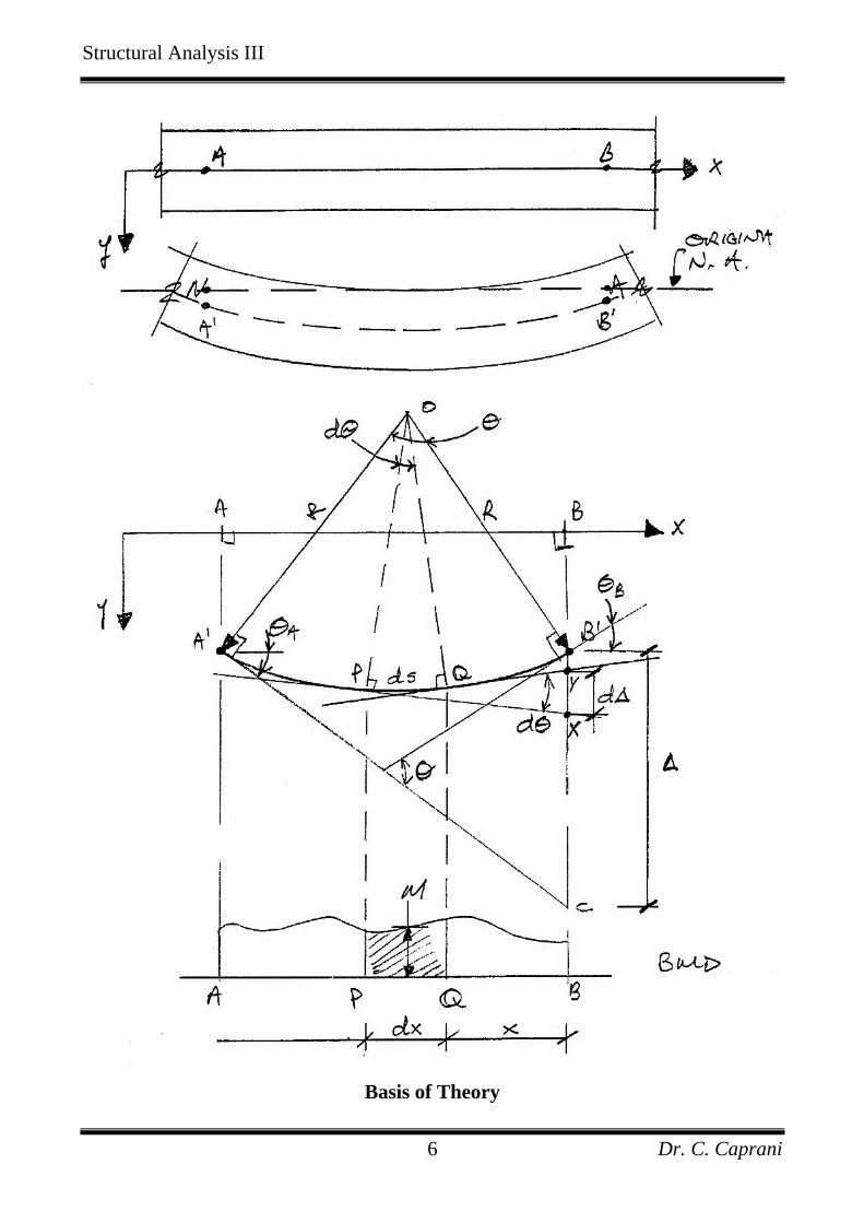
We consider a length of beam AB in its undeformed and deformed state, as shown on
the next page. Studying this diagram carefully, we note:
1. AB is the original unloaded length of the beam and A’B’ is the deflected
position of AB when loaded.
2. The angle subtended at the centre of the arc A’OB’ is θ and is the change in
curvature from A’ to B’.
3. PQ is a very short length of the beam, measured as ds along the curve and dx
along the x-axis.
4. dθ is the angle subtended at the centre of the arc . ds
5. dθ is the change in curvature from P to Q.
6. M is the average bending moment over the portion between P and Q. dx
7. The distance is known as the vertical intercept and is the distance from B’ to
the produced tangent to the curve at A’ which crosses under B’ at C. It is
measured perpendicular to the undeformed neutral axis (i.e. the x-axis) and so
is ‘vertical’.
∆
Dr. C. Caprani 5
Structural Analysis III
Basis of Theory
Dr. C. Caprani 6

Structural Analysis III
2.2 Mohr’s First Theorem (Mohr I)
Development
Noting that the angles are always measured in radians, we have:
ds R d
dsRd
θ
θ
= ⋅
∴ =
From the Euler-Bernoulli Theory of Bending, we know:
1 MR EI=
Hence:
Md dsEI
θ = ⋅
But for small deflections, the chord and arc length are similar, i.e. , giving: ds dx≈
Md dxEI
θ = ⋅
The total change in rotation between A and B is thus:
B B
A A
Md dxEI
θ =∫ ∫
Dr. C. Caprani 7

Structural Analysis III
The term M EI is the curvature and the diagram of this term as it changes along a
beam is the curvature diagram (or more simply the M EI diagram). Thus we have:
B
BA B AA
Md dxEI
θ θ θ= − = ∫
This is interpreted as:
[ ]Change in slope Area of diagramAB
AB
MEI
⎡ ⎤= ⎢ ⎥⎣ ⎦
This is Mohr’s First Theorem (Mohr I):
The change in slope over any length of a member subjected to bending is equal
to the area of the curvature diagram over that length.
Usually the beam is prismatic and so E and I do not change over the length AB,
whereas the bending moment M will change. Thus:
1 B
ABA
M dxEI
θ = ∫
[ ] [ ]Area of diagramChange in slope AB
AB
MEI
=
Dr. C. Caprani 8

Structural Analysis III
Example 1
For the cantilever beam shown, we can find the rotation at B easily:
Thus, from Mohr I, we have:
[ ]Change in slope Area of diagram
12
ABAB
B A
MEI
PLLEI
θ θ
⎡ ⎤= ⎢ ⎥⎣ ⎦
− = ⋅ ⋅
Since the rotation at A is zero (it is a fixed support), i.e. 0Aθ = , we have:
2
2BPLEI
θ =
Dr. C. Caprani 9

Structural Analysis III
2.3 Mohr’s Second Theorem (Mohr II)
Development
From the main diagram, we can see that:
d x dθ∆ = ⋅
But, as we know from previous,
Md dxEI
θ = ⋅
Thus:
Md x dxEI
∆ = ⋅ ⋅
And so for the portion AB, we have:
First moment of diagram about
B B
A A
B
BAA
Md x dxEI
M dx xEI
M BEI
∆ = ⋅ ⋅
⎡ ⎤∆ = ⋅⎢ ⎥
⎣ ⎦
=
∫ ∫
∫
This is easily interpreted as:
Dr. C. Caprani 10
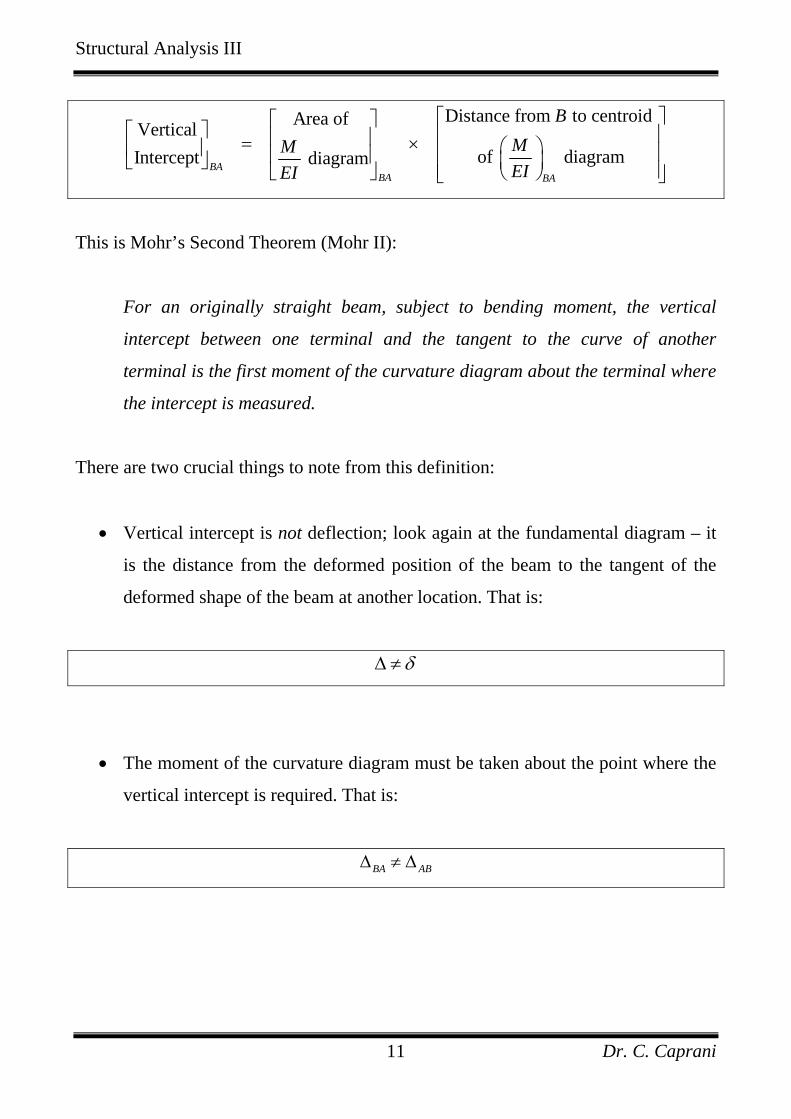
Structural Analysis III
Distance from to centroid Area of Vertical
of diagramIntercept diagramBABA BA
BMMEIEI
⎡ ⎤⎡ ⎤⎡ ⎤ ⎢ ⎥⎢ ⎥= × ⎛ ⎞⎢ ⎥ ⎢ ⎥⎢ ⎥ ⎜ ⎟⎣ ⎦ ⎢ ⎥⎣ ⎦ ⎝ ⎠⎣ ⎦
This is Mohr’s Second Theorem (Mohr II):
For an originally straight beam, subject to bending moment, the vertical
intercept between one terminal and the tangent to the curve of another
terminal is the first moment of the curvature diagram about the terminal where
the intercept is measured.
There are two crucial things to note from this definition:
• Vertical intercept is not deflection; look again at the fundamental diagram – it
is the distance from the deformed position of the beam to the tangent of the
deformed shape of the beam at another location. That is:
δ∆ ≠
• The moment of the curvature diagram must be taken about the point where the
vertical intercept is required. That is:
BA AB∆ ≠ ∆
Dr. C. Caprani 11

Structural Analysis III
Example 2
For the cantilever beam, we can find the defection at B since the produced tangent at
A is horizontal, i.e. 0Aθ = . Thus it can be used to measure deflections from:
Thus, from Mohr II, we have:
1 22 3BA
PL LLEI
⎡ ⎤ ⎡ ⎤∆ = ⋅ ⋅⎢ ⎥ ⎢ ⎥⎣ ⎦ ⎣ ⎦
And so the deflection at B is:
3
3BPLEI
δ =
Dr. C. Caprani 12

Structural Analysis III
2.4 Area Properties
These are well known for triangular and rectangular areas. For parabolic areas we
have:
Shape Area Centroid
23
A xy= 12
x x=
23
A xy= 58
x x=
13
A xy= 34
x x=
Dr. C. Caprani 13

Structural Analysis III
3. Application to Determinate Structures
3.1 Basic Examples
Example 3
For the following beam, find Bδ , Cδ , Bθ and Cθ given the section dimensions shown
and 210 kN/mmE = .
To be done in class.
Dr. C. Caprani 14
Structural Analysis III
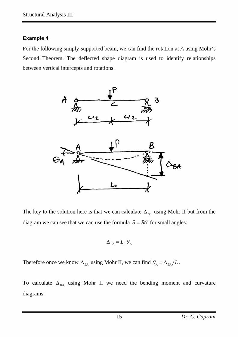
Example 4
For the following simply-supported beam, we can find the rotation at A using Mohr’s
Second Theorem. The deflected shape diagram is used to identify relationships
between vertical intercepts and rotations:
The key to the solution here is that we can calculate BA∆ using Mohr II but from the
diagram we can see that we can use the formula S Rθ= for small angles:
BA AL θ∆ = ⋅
Therefore once we know BA∆ using Mohr II, we can find A BA Lθ = ∆ .
To calculate BA∆ using Mohr II we need the bending moment and curvature
diagrams:
Dr. C. Caprani 15

Structural Analysis III
Thus, from Mohr II, we have:
3
12 4 2
16
BAPL LLEI
PLEI
⎡ ⎤ ⎡ ⎤∆ = ⋅ ⋅⎢ ⎥ ⎢ ⎥⎣ ⎦ ⎣ ⎦
=
But, BA L Aθ∆ = ⋅ and so we have:
2
16
BAA L
PLEI
θ ∆=
=
Dr. C. Caprani 16

Structural Analysis III
3.2 Finding Deflections
General Procedure
To find the deflection at any location x from a support use the following relationships
between rotations and vertical intercepts:
Thus we:
1. Find the rotation at the support using Mohr II as before;
2. For the location x, and from the diagram we have:
x B xx Bδ θ= ⋅ − ∆
Dr. C. Caprani 17

Structural Analysis III
Maximum Deflection
To find the maximum deflection we first need to find the location at which this
occurs. We know from beam theory that:
ddxθδ =
Hence, from basic calculus, the maximum deflection occurs at a rotation, 0θ = :
To find where the rotation is zero:
1. Calculate a rotation at some point, say support A, using Mohr II say;
2. Using Mohr I, determine at what distance from the point of known rotation (A)
the change in rotation (Mohr I), Axdθ equals the known rotation ( Aθ ).
3. This is the point of maximum deflection since:
0A Ax A Adθ θ θ θ− = − =
Dr. C. Caprani 18

Structural Analysis III
Example 5
For the following beam of constant EI:
(a) Determine Aθ , Bθ and Cδ ;
(b) What is the maximum deflection and where is it located?
Give your answers in terms of EI.
The first step is to determine the BMD and draw the deflected shape diagram with
rotations and tangents indicated:
Dr. C. Caprani 19

Structural Analysis III
Rotations at A and B
To calculate the rotations, we need to calculate the vertical intercepts and use the fact
that the intercept is length times rotation. Thus, for the rotation at B:
2 1 4 12 2 2 43 2 3 2
4 203 3
88
AB
AB
EI M
M
MM
M
EI
⎛ ⎞⎛ ⎞ ⎛ ⎞⎛ ⎞∆ = ⋅ ⋅ ⋅ + + ⋅ ⋅⎜ ⎟⎜ ⎟ ⎜ ⎟⎜ ⎟⎝ ⎠⎝ ⎠ ⎝ ⎠⎝ ⎠
⎛ ⎞= +⎜ ⎟⎝ ⎠
=
∴∆ =
But, we also know that 6AB Bθ∆ = . Hence:
86
4 1.333
B
B
MEI
M MEI E
θ
θ
=
I∴ = =
Similarly for the rotation at A:
2 1 1 14 4 4 2 23 2 3 2
16 143 3
1010
BA
BA
EI M
M
MM
M
EI
⎛ ⎞⎛ ⎞ ⎛ ⎞⎛ ⎞∆ = ⋅ ⋅ ⋅ + + ⋅ ⋅ ⋅⎜ ⎟⎜ ⎟ ⎜ ⎟⎜ ⎟⎝ ⎠⎝ ⎠ ⎝ ⎠⎝ ⎠
⎛ ⎞= +⎜ ⎟⎝ ⎠
=
∴∆ =
But, we also know that 6BA Aθ∆ = and so:
Dr. C. Caprani 20

Structural Analysis III
106 A
MEI
θ =
5 1.673A
M MEI E
θI
∴ = =
Deflection at C
To find the deflection at C, we use the vertical intercept CB∆ and Bθ :
From the figure, we see:
4C B CBδ θ= − ∆
And so from the BMD and rotation at B:
( ) 1 44 1.33 4
2 3
2.665
C
C
EI M M
MEI
δ
δ
⎛ ⎞⎛= − ⋅ ⋅⎜ ⎟⎜⎝ ⎠⎝
⎞⎟⎠
∴ =
Dr. C. Caprani 21

Structural Analysis III
Maximum Deflection
The first step in finding the maximum deflection is to locate it. We know tow things:
1. Maximum deflection occurs where there is zero rotation;
2. Maximum deflection is always close to the centre of the span.
Based on these facts, we work with Mohr I to find the point of zero rotation, which
will be located between B and C, as follows:
Change in rotation 0B Bθ θ= − =
But since we know that the change in rotation is also the area of the M EI diagram
we need to find the point x where the area of the M EI diagram is equal to Bθ :
Thus:
( )
2
104 2
8
B
B
xEI M
xEI M
θ
θ
⎛ ⎞ x− = ⋅ ⋅ ⋅⎜ ⎟⎝ ⎠
=
But we know that 1.33B
MEI
θ = , hence:
Dr. C. Caprani 22

Structural Analysis III
2
2
1.338
10.663.265 m from or 2.735 m from
M xEI MEI
xx B A
⎛ ⎞ =⎜ ⎟⎝ ⎠
==
So we can see that the maximum deflection is 265 mm shifted from the centre of the
beam towards the load. Once we know where the maximum deflection is, we can
calculate is based on the following diagram:
Thus:
max B xx Bδ θ= − ∆
( )
( )
2
max
max
1.338 3
4.342 1.450
2.892
x xEI x M M
MMEI
δ
δ
⎛ ⎞⎛ ⎞= − ⎜ ⎟⎜ ⎟⎝ ⎠⎝ ⎠= −
=
And since 53.4 kNmM = , max
154.4EI
δ = .
Dr. C. Caprani 23

Structural Analysis III
3.3 Problems
1. For the beam of Example 3, using only Mohr’s First Theorem, show that the
rotation at support B is equal in magnitude but not direction to that at A.
2. For the following beam, of dimensions 150 mmb = and and 225 mmd =210 kN/mmE = , show that and 47 10 radsBθ
−= × 9.36 mmBδ = .
3. For a cantilever AB of length L and stiffness EI, subjected to a UDL, show that:
3 4
;6 8B BwL wLEI E
θ δ= =I
4. For a simply-supported beam AB with a point load at mid span (C), show that:
3
48CPL
EIδ =
5. For a simply-supported beam AB of length L and stiffness EI, subjected to a UDL,
show that:
3 3 5; ;
24 24 384A B CwL wL wL4
EI EIθ θ δ= = − =
EI
Dr. C. Caprani 24

Structural Analysis III
4. Application to Indeterminate Structures
4.1 Basis of Approach
Using the principle of superposition we will separate indeterminate structures into a
primary and reactant structures.
For these structures we will calculate the deflections at a point for which the
deflection is known in the original structure.
We will then use compatibility of displacement to equate the two calculated
deflections to the known deflection in the original structure.
Doing so will yield the value of the redundant reaction chosen for the reactant
structure.
Once this is known all other load effects (bending, shear, deflections, rotations) can
be calculated.
See the handout on Compatibility of Displacement and the Principle of Superposition
for more on this approach.
Dr. C. Caprani 25

Structural Analysis III
4.2 Example 6: Propped Cantilever
For the following prismatic beam, find the maximum deflection in span AB and the
deflection at C in terms of EI.
Find the reaction at B
Since this is an indeterminate structure, we first need to solve for one of the unknown
reactions. Choosing BV as our redundant reaction, using the principle of
superposition, we can split the structure up as shown:
(a) = (b) + (c)
In which R is the value of the chosen redundant.
Dr. C. Caprani 26

Structural Analysis III
In the final structure (a) we know that the deflection at B, Bδ , must be zero as it is a
roller support. So from the BMD that results from the superposition of structures (b)
and (c) we can calculate Bδ in terms of R and solve since 0Bδ = .
We have from Mohr II:
( )
( ) ( )
1 2 1 22 200 2 2 4 4 42 3 2 3
2000 643 3
1 2000 643
BAb c
EI R
R
R
⎡ ⎤ ⎡ ⎤⎛ ⎞⎛ ⎞ ⎛ ⎞⎛∆ = ⋅ ⋅ + ⋅ + − ⋅ ⋅ ⋅⎜ ⎟⎜ ⎟ ⎜ ⎟⎜⎞⎟⎢ ⎥ ⎢ ⎥⎝ ⎠⎝ ⎠ ⎝ ⎠⎝ ⎠⎣ ⎦ ⎣ ⎦
= −
= −
But since 0Aθ = , B BAδ = ∆ and so we have:
( )
01 2000 64 03
64 200031.25 kN
BAEI
R
RR
∆ =
− =
== +
Dr. C. Caprani 27

Structural Analysis III
The positive sign for R means that the direction we originally assumed for it
(upwards) was correct.
At this point the final BMD can be drawn but since its shape would be more complex
we continue to operate using the structure (b) and (c) BMDs.
Find the location of the maximum deflection
This is the next step in determining the maximum deflection in span AB. Using the
knowledge that the tangent at A is horizontal, i.e. 0Aθ = , we look for the distance x
from A that satisfies:
0Ax A xdθ θ θ= − =
By inspection on the deflected shape, it is apparent that the maximum deflection
occurs to the right of the point load. Hence we have the following:
Dr. C. Caprani 28

Structural Analysis III
So using Mohr I we calculate the change in rotation by finding the area of the
curvature diagram between A and x. The diagram is split for ease:
The Area 1 is trivial:
11 200 20022
AEI EI
= ⋅ ⋅ =
For Area 2, we need the height first which is:
24 4 4 125 125 125 125
4 4x Rh x
EI EI EI E− ⋅ −
= ⋅ = = −I
And so the area itself is:
2125 125A x xEI EI
⎡ ⎤= ⋅ −⎢ ⎥⎣ ⎦
For Area 3 the height is:
3125 125 125 125h x xEI EI EI EI
⎡ ⎤= − − =⎢ ⎥⎣ ⎦
Dr. C. Caprani 29

Structural Analysis III
And so the area is:
21 1252
A x xEI
= ⋅ ⋅
Being careful of the signs for the curvatures, the total area is:
1 2 3
2
2
125 125200 1254 8
125 125 125 2008 4
AxEId A A A
x x x
x x
θ = − + +
⎛ ⎞= − + − +⎜ ⎟⎝ ⎠
⎛ ⎞= − + −⎜ ⎟⎝ ⎠
Setting this equal to zero to find the location of the maximum deflection, we have:
2
2
125 125 200 08
5 40 64
x x
0x x
− + − =
− + =
Thus, 5.89 mx = or 2.21 mx = . Since we are dealing with the portion AB,
2.21 mx = .
Find the maximum deflection
Since the tangent at both A and x are horizontal, i.e. 0Aθ = and 0xθ = , the deflection
is given by:
max xAδ = ∆
Using Mohr II and Areas 1, 2 and 3 as previous, we have:
Dr. C. Caprani 30

Structural Analysis III
Area
1
1 1200 1.543
308.67
A xEI
EI
= − ⋅
= −
Area
2
24 2.21 4 55.94
4Rh
EI EI−
= ⋅ =
2 255.94 2.212.21
2136.61
A xEI
EI
= ⋅ ⋅
=
Area
3
3125 69.062.21hEI EI
= ⋅ =
3 31 69.062.21 1.4732
112.43
A xEI
EI
⎡ ⎤= ⋅ ⋅ ⋅⎢ ⎥⎣ ⎦
=
Thus:
max
max
308.67 136.61 112.4359.63
xBEI EI
EI
δ
δ
∆ = = − + +−
⇒ =
The negative sign indicates that the negative bending moment diagram dominates, i.e.
the hogging of the cantilever is pushing the deflection downwards.
Dr. C. Caprani 31
Structural Analysis III
Find the deflection at C
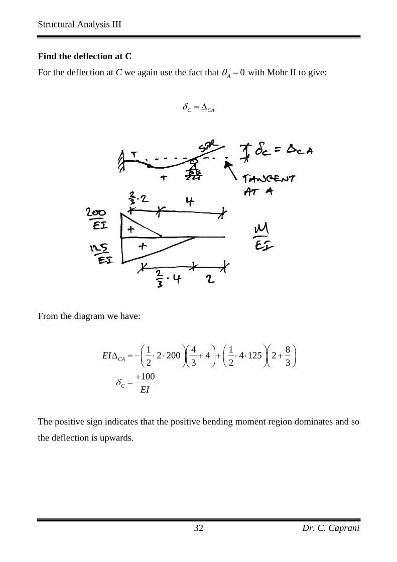
For the deflection at C we again use the fact that 0Aθ = with Mohr II to give:
C CAδ = ∆
From the diagram we have:
1 4 12 200 4 4 125 22 3 2
100
CA
C
EI 83
EIδ
⎛ ⎞⎛ ⎞ ⎛ ⎞⎛∆ = − ⋅ ⋅ + + ⋅ ⋅ +⎜ ⎟⎜ ⎟ ⎜ ⎟⎜⎝ ⎠⎝ ⎠ ⎝ ⎠⎝
+=
⎞⎟⎠
The positive sign indicates that the positive bending moment region dominates and so
the deflection is upwards.
Dr. C. Caprani 32

Structural Analysis III
4.3 Example 7: 2-Span Beam
For the following beam of constant EI, using Mohr’s theorems:
(a) Draw the bending moment diagram;
(b) Determine, Dδ and Eδ ;
Give your answers in terms of EI.
In the last example we knew the rotation at A and this made finding the deflection at
the redundant support relatively easy. Once again we will choose a redundant
support, in this case the support at B.
In the present example, we do not know the rotation at A – it must be calculated – and
so finding the deflection at B is more involved. We can certainly use compatibility of
displacement at B, but in doing so we will have to calculate the vertical intercept
from B to A, , twice. Therefore, to save effort, we use BA∆ BA∆ as the measure which
we apply compatibility of displacement to. We will calculate BA∆ through calculation
of Aθ (and using the small angle approximation) and through direct calculation from
the bending moment diagram. We will then have an equation in R which can be
solved.
Dr. C. Caprani 33

Structural Analysis III
Rotation at A
Breaking the structure up into primary and redundant structures:
So we can see that the final rotation at A is:
P RA A Aθ θ θ= +
To find the rotation at A in the primary structure, consider the following:
By Mohr II we have:
Dr. C. Caprani 34

Structural Analysis III
( )( )240 9 6 12960CAEI∆ = ⋅ =
But we know, from the small angle approximation, 12CA Aθ∆ = , hence:
12960 108012 12
1080
P CAA
PA
EI
EI
θ
θ
∆= = =
∴ =
To find the rotation at A for the reactant structure, we have:
( )1 12 3 6 1082CAEI R⎛ ⎞∆ = ⋅ ⋅ =⎜ ⎟
⎝ ⎠R
12CA Aθ∆ =
108 912 129
R CAA
RA
REI R
REI
θ
θ
∆= = =
∴ = −
Dr. C. Caprani 35

Structural Analysis III
Notice that we assign a negative sign to the reactant rotation at A since it is in the
opposite sense to the primary rotation (which we expect to dominate).
Thus, we have:
1080 9
P RA A A
REI EI
θ θ θ= +
= −
Vertical Intercept from B to A
The second part of the calculation is to find BA∆ directly from calculation of the
curvature diagram:
Thus we have:
( )1 1 3 16 3 6 240 3 3 240 32 3 2 2BAEI R⎛ ⎞⎛ ⎞ ⎛ ⎞ ⎛ ⎞⎛∆ = − ⋅ ⋅ ⋅ + ⋅ + ⋅ ⋅ +⎜ ⎟⎜ ⎟ ⎜ ⎟ ⎜ ⎟⎜
⎝ ⎠⎝ ⎠ ⎝ ⎠ ⎝ ⎠⎝33⎞⎟⎠
Dr. C. Caprani 36

Structural Analysis III
18 1080 1440
2520 18BA
BA
EI RR
EI
∆ = − + +−
∴∆ =
Solution for R
Now we recognize that 6BA Aθ∆ = by compatibility of displacement, and so:
( )
2520 18 1080 96
2520 18 6 1080 936 3960
110 kN
R REI EI EI
R RRR
− ⎛ ⎞= −⎜ ⎟⎝ ⎠
− = −
==
Solution to Part (a)
With this we can immediately solve for the final bending moment diagram by
superposition of the primary and reactant BMDs:
Dr. C. Caprani 37

Structural Analysis III
Solution to Part (b)
We are asked to calculate the deflection at D and E. However, since the beam is
symmetrical D Eδ δ= and so we need only calculate one of them – say Dδ . Using the
(now standard) diagram for the calculation of deflection:
( )9 1101080 90A EI EI E
θ = − =I
1 33 75 112.53 3DAEI ⎛ ⎞⎛ ⎞∆ = ⋅ ⋅ =⎜ ⎟⎜ ⎟
⎝ ⎠⎝ ⎠
But 3D A DAδ θ= − ∆ , thus:
( )3 90 112.5157.5
157.5
D
D E
EI
EI
δ
δ δ
= −
=
= =
Dr. C. Caprani 38

Structural Analysis III
4.4 Example 8: Simple Frame
For the following frame of constant 240 MNmEI = , using Mohr’s theorems:
(a) Draw the bending moment and shear force diagram;
(b) Determine the horizontal deflection at E.
Part (a)
Solve for a Redundant
As with the beams, we split the structure into primary and reactant structures:
Dr. C. Caprani 39

Structural Analysis III
We also need to draw the deflected shape diagram of the original structure to identify
displacements that we can use:
To solve for R we could use any known displacement. In this case we will use the
vertical intercept as shown, because: DB∆
• We can determine for the original structure in terms of R using Mohr’s
Second Theorem;
DB∆
• We see that 6DB Bθ∆ = and so using Mohr’s First Theorem for the original
structure we will find Bθ , again in terms of R;
• We equate the two methods of calculating DB∆ (both are in terms of R) and
solve for R.
Dr. C. Caprani 40
Structural Analysis III
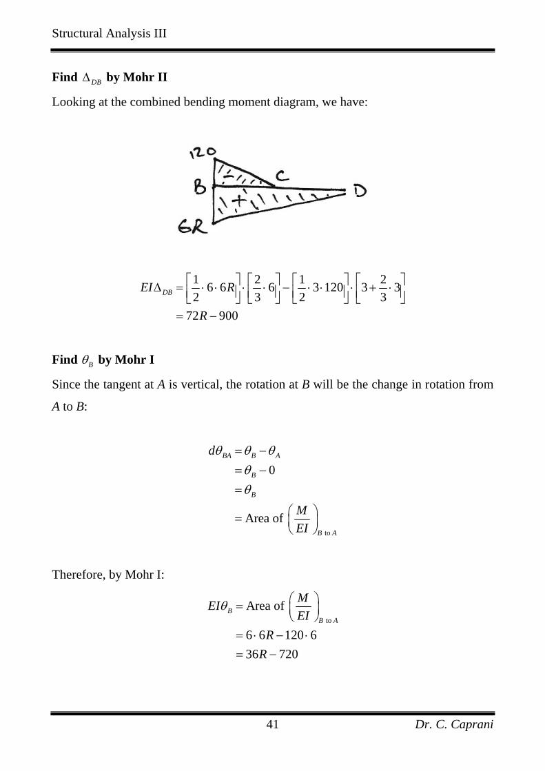
Find by Mohr II DB∆
Looking at the combined bending moment diagram, we have:
1 2 16 6 6 3 120 3 32 3 2
72 900
DBEI R
R
⎡ ⎤ ⎡ ⎤ ⎡ ⎤ ⎡∆ = ⋅ ⋅ ⋅ ⋅ − ⋅ ⋅ ⋅ + ⋅⎢ ⎥ ⎢ ⎥ ⎢ ⎥ ⎢⎣ ⎦ ⎣ ⎦ ⎣ ⎦ ⎣= −
23
⎤⎥⎦
Find Bθ by Mohr I
Since the tangent at A is vertical, the rotation at B will be the change in rotation from
A to B:
to
0
Area of
BA B A
B
B
B A
d
MEI
θ θ θθθ
= −= −=
⎛ ⎞= ⎜ ⎟⎝ ⎠
Therefore, by Mohr I:
to
Area of
6 6 120 636 720
BB A
MEIEI
RR
θ ⎛ ⎞= ⎜ ⎟⎝ ⎠
= ⋅ − ⋅= −
Dr. C. Caprani 41

Structural Analysis III
Equate and Solve for R
As identified previously:
[ ]6
72 900 6 36 72018.13 kN
DB B
R RR
θ∆ =
− = −
=
Diagrams
Knowing R we can then solve for the reactions, bending moment and shear force
diagrams. The results are:
Dr. C. Caprani 42

Structural Analysis III
Part (b)
The movement at E is comprised of Dxδ and 6 Dθ as shown in the deflection diagram.
These are found as:
• Since the length of member BD doesn’t change, Dx Bxδ δ= . Further, by Mohr II,
Bx BAδ = ∆ ;
• By Mohr I, D B d BDθ θ θ= − , that is, the rotation at D is the rotation at B minus
the change in rotation from B to D:
So we have:
[ ][ ] [ ][ ]6 6 3 120 6 3202.5
BAEI R∆ = ⋅ − ⋅
= −
1 16 6 120 32 2
146.25
BDEId Rθ ⎡ ⎤ ⎡ ⎤= ⋅ ⋅ − ⋅ ⋅⎢ ⎥ ⎢ ⎥⎣ ⎦ ⎣ ⎦=
Notice that we still use the primary and reactant diagrams even though we know R.
We do this because the shapes and distances are simpler to deal with.
From before we know:
Dr. C. Caprani 43

Structural Analysis III
36 720 67.5BEI Rθ = − =
Thus, we have:
67.5 146.2578.75
D B BEI EI d Dθ θ θ= −= −= −
The minus indicates that it is a rotation in opposite direction to that of Bθ which is
clear from the previous diagram. Since we have taken account of the sense of the
rotation, we are only interested in its absolute value. A similar argument applies to
the minus sign for the deflection at B. Therefore:
6202.5 78.756
675
Ex Bx D
EI EI
EI
δ δ θ= +
= + ⋅
=
Using 240 MNmEI = gives 16.9 mmExδ = .
Dr. C. Caprani 44

Structural Analysis III
4.5 Example 9: Complex Frame
For the following frame of constant 240 MNmEI = , using Mohr’s theorems:
(a) Determine the reactions and draw the bending moment diagram;
(b) Determine the horizontal deflection at D.
In this frame we have the following added complexities:
• There is a UDL and a point load which leads to a mix of parabolic, triangular
and rectangular BMDs;
• There is a different EI value for different parts of the frame – we must take this
into account when performing calculations and not just consider the M diagram
but the M EI diagram as per Mohr’s Theorems.
Dr. C. Caprani 45

Structural Analysis III
Solve for a Redundant
As is usual, we split the frame up:
Next we draw the deflected shape diagram of the original structure to identify
displacements that we can use:
Dr. C. Caprani 46

Structural Analysis III
To solve for R we will use the vertical intercept DC∆ as shown, because:
• We can determine DC∆ for the original structure in terms of R using Mohr II;
• We see that 6DC Cθ∆ = and so using Mohr I for the original structure we will
find Bθ , again in terms of R;
• As usual, we equate the two methods of calculating DC∆ (both are in terms of
R) and solve for R.
Dr. C. Caprani 47

Structural Analysis III
The Rotation at C
To find the rotation at C, we must base our thoughts on the fact that we are only able
to calculate the change in rotation from one point to another using Mohr I. Thus we
identify that we know the rotation at A is zero – since it is a fixed support – and we
can find the change in rotation from A to C, using Mohr I. Therefore:
to
0A C C A
C
C
dθ θ θθθ
= −= −=
At this point we must recognize that since the frame is swaying to the right, the
bending moment on the outside ‘dominates’ (as we saw for the maximum deflection
calculation in Example 6). The change in rotation is the difference of the absolute
values of the two diagrams, hence we have, from the figure, and from Mohr I:
( ) ( ) to
1360 8 240 4 6 82
3360 483360 48
A C
C
C
EId R
EI RR
EI
θ
θ
θ
⎛ ⎞= ⋅ + ⋅ ⋅ − ⋅⎜ ⎟⎝ ⎠
= −
−∴ =
Dr. C. Caprani 48

Structural Analysis III
The Vertical Intercept DC
Using Mohr II and from the figure we have:
1 2 1 31.5 6 6 6 6 360 62 3 3 4
1.5 72 324048 2160
DC
DC
DC
EI R
EI RR
EI
⎡ ⎤ ⎡⎛ ⎞⎛ ⎞ ⎛ ⎞⎛ ⎞⎤∆ = ⋅ ⋅ ⋅ − ⋅ ⋅ ⋅⎜ ⎟⎜ ⎟ ⎜ ⎟⎜ ⎟⎢ ⎥ ⎢⎝ ⎠⎝ ⎠ ⎝ ⎠⎝ ⎠⎣ ⎦ ⎣∆ = −
−∴∆ =
⎥⎦
Note that to have neglected the different EI value for member CD would change the
result significantly.
Solve for R
By compatibility of displacement we have 6DC Cθ∆ = and so:
( )48 2160 6 3360 48
336 2232066.43 kN
R RRR
− = −
==
With R now known we can calculate the horizontal deflection at D.
Dr. C. Caprani 49

Structural Analysis III
Part (b) - Horizontal Deflection at D
From the deflected shape diagram of the final frame and by neglecting axial
deformation of member CD, we see that the horizontal displacement at D must be the
same as that at C. Note that it is easier at this stage to work with the simpler shape of
the separate primary and reactant BMDs. Using Mohr II we can find Cxδ as shown:
( )( ) ( )( ) 1 26 8 4 360 8 4 4 240 4 42 3
192 14720
BAEI R
R
⎡ ⎤⎛ ⎞⎛∆ = ⋅ − ⋅ + ⋅ ⋅ + ⋅⎡ ⎤ ⎜ ⎟⎜⎞⎟⎢ ⎥⎣ ⎦ ⎝ ⎠⎝ ⎠⎣ ⎦
= −
Now substituting and 66.4 kNR = Dx Cx BAδ δ= = ∆ :
1971.2 49.3 mmDx EIδ −
= = →
Note that the negative sign indicates that the bending on the outside of the frame
dominates, pushing the frame to the right as we expected.
Dr. C. Caprani 50

Structural Analysis III
Part (a) – Reactions and Bending Moment Diagram
Reactions
Taking the whole frame, and showing the calculated value for R, we have:
( )
2
0 20 6 66.4 0 53.6 kN
0 60 0 60 kN
6M about 0 66.4 6 20 60 4 0 201.6 kNm2
y A A
x A A
A A
F V V
F H H
A M M
= ∴ ⋅ − − = ∴ =
= ∴ − = ∴ =
= ∴ + ⋅ − ⋅ − ⋅ = ∴ = +
∑
∑
∑
↑
←
Note that it is easier to use the superposition of the primary and reactant BMDs to
find the moment at A:
( )6 66.4 600 201.6 kNmAM = − = −
The negative sign indicate the moment on the outside of the frame dominates and so
tension is on the left.
Dr. C. Caprani 51

Structural Analysis III
Bending Moment Diagram
We find the moments at salient points:
2
M about 0
620 66.4 6 02
38.4 kNm
C
C
C
M
M
=
∴ + ⋅ − ⋅ =
∴ = +
∑
And so tension is on the bottom at C.
The moment at B is most easily found from superposition of the BMDs as before:
( )6 66.4 360 38.4 kNmBM = − =
And so tension is on the inside of the frame at B. Lastly we must find the value of
maximum moment in span CD. The position of zero shear is found as:
53.6 2.68 m20
x = =
And so the distance from D is:
6 2.68 3.32 m− =
The maximum moment is thus found from a free body diagram as follows:
Dr. C. Caprani 52

Structural Analysis III
2
max
M about 0
3.3220 66.4 3.32 02
110.2 kNmC
X
M
M
=
∴ + ⋅ − ⋅ =
∴ = +
∑
And so tension is on the bottom as
expected.
Summary of Solution
In summary the final solution for this frame is:
Dr. C. Caprani 53

Structural Analysis III
4.6 Problems
1. For the following prismatic beam, find the bending moment diagram and the
rotation at E in terms of EI.
2. For the following prismatic beam, find the bending moment diagram and the
rotation at C in terms of EI. (Autumn 2007)
3. For the following prismatic frame, find the bending moment and shear force
diagrams and the horizontal deflection at E in terms of EI.
Dr. C. Caprani 54

Structural Analysis III
4. For the following prismatic frame, find the bending moment diagram and the
horizontal deflection at D in terms of EI. (Summer 2006)
5. For the following prismatic frame, find the bending moment diagram and the
horizontal defection at C in terms of EI. (Summer 2007)
Dr. C. Caprani 55

Structural Analysis III
6. Draw the bending moment diagram and find the maximum deflection for the
following beam. Take . (Semester 1 2007/8) 320 10 kNmEI = × 2
A
HINGE
40 kN
2 m 2 m2 m4 m
B C D E
7. Draw the bending moment diagram and determine the horizontal deflection at D
for the following frame. Take 34 10 kNm2EI = × . (Summer 1998)
Dr. C. Caprani 56