strong sure screening of ultra-high dimensional cate ... · strong sure screening of ultra-high...

arX

iv:1

801.

0353

9v2

[st

at.M

E]

30

Jan

2018

Strong Sure Screening of Ultra-high Dimensional Cate-

gorical Data

Randall Reese1, Xiaotian Dai1, & Guifang Fu1

1Department of Mathematics and Statistics, Utah State University

Feature screening for ultra high dimensional feature spaces plays a critical role in the anal-

ysis of data sets whose predictors exponentially exceed the number of observations. Such

data sets are becoming increasingly prevalent in areas such as bioinformatics, medical imag-

ing, and social network analysis. Frequently, these data sets have both categorical response

and categorical covariates, yet extant feature screening literature rarely considers such data

types. We propose a new screening procedure rooted in the Cochran-Armitage trend test.

Our method is specifically applicable for data where both the response and predictors are

categorical. Under a set of reasonable conditions, we demonstrate that our screening proce-

dure has the strong sure screening property, which extends the seminal results of Fan and

Lv. A series of four simulations are used to investigate the performance of our method rela-

tive to three other screening methods. We also apply a two-stage iterative approach to a real

data example by first employing our proposed method, and then further screening a subset

of selected covariates using lasso, adaptive-lasso and elastic net regularization.

1

http://arxiv.org/abs/1801.03539v2

1 Introduction

With the ever increasing prevalence of high and ultra-high dimensional data in fields such as bioin-

formatics, medical imaging and tomography, finance, and sensor systems, there has arisen an ac-

companying need for methods of analyzing said data. Developing methods for the analysis of such

data requires methods that are not only statistically sound and accurate, but that moreover are com-

putationally tractable. 11 provides us with a holistic overview of challenges in high dimensional

data analysis. 16 and 15 expand upon the statistical challenges of high dimensional data analysis.

One fundamental pursuit that has received considerable attention in recent literature is vari-

able selection or feature screening. Based on the concept of sparsity, feature screening aims to

select a relatively small set of important variables from an overall large feature space. For lexical

consistency, given n samples for each of p variables, we will use the term “high dimensional" to

mean p = O(nξ) for some ξ > 0, and the term “ultra-high dimensional" to mean log(p) = O(nξ)

for some ξ > 0.

A fundamental challenge of variable selection in high and ultra-high dimensional feature

spaces comes from the existence of an immense amount of noise features. This preponderance

of noise can lead to an accumulation of aggregate error rates for certain selection methods. For

example, as discussed in 13, when using a discriminant analysis rule such as LDA or QDA, the pop-

ulation mean vectors are estimated from the observed sample. In cases where the dimensionality

is high, although individual components of the population mean vectors can be estimated with suf-

ficient accuracy, the aggregated estimation error can be very large. This will obviously adversely

2

affect the misclassification rate.

Cases such as the one discussed above introduce us to the motivation behind dimension

reduction techniques like feature screening. A multiplicity of methods for variable selection in

high dimensional feature spaces have been proposed. Methods such as ridge regression [20] and

LASSO [38] were early methods that employed penalized least squares. Similar penalized pseudo-

likelihood methods such as the smoothly clipped absolute deviation (SCAD) method [2] the least

angle regression (LARS) algorithm [12] and the Dantzig selector [6] soon thereafter followed.

However, as 18 point out, the computation inherent in these aforementioned methods impedes

our ability to directly apply them to ultra-high dimensional feature spaces. The simultaneous

challenges of computational expediency, statistical accuracy, and algorithmic stability often make

such approaches intractable.

In their pioneering paper, 17 lay the ground work for sure independent screening (SIS) feature

screening in ultra-high dimensional feature spaces and established the conceptual underpinnings

of much of the literature that would thereafter follow. This new era of research sought to overcome

the computational limitations of the previous approaches and develop a repertoire of methods vi-

able for the rapidly growing (both in size and totality) ultra-high dimensional data sets requiring

analysis.

Most early approaches stemming from 17 were constructed under assumptions on various

forms of linear models between the response and the covariates. In that original paper itself,

3

Fan and Lv assumed a strict linear model with all covariates and the response being normally dis-

tributed. 18 assume a generalized linear model, as does the maximum marginal likelihood estimator

(MMLE) method of 19. 40 further explored feature selection in the context of the generalized linear

model. Recent publications have proposed feature screening methods that are non-parametric or

model-free, where the assumptions on the underlying model between predictor and response are

relaxed or even removed. [See e.g. 14; 42; 27 ; 4; 9]. We will further address the distance correlation

based method of 27 later in this paper.

Even though these aforementioned methods relax or remove assumptions on the relationship

between covariate and response, most SIS-based procedures still tacitly assume that the predictor

variables are continuous. Notably, this implicit assumption of continuity of the predictors can be

limiting, since ultrahigh dimensional data with discrete predictors and discrete responses are rather

ubiquitous in practice. (For example, the fields of bioinformatics and text mining commonly have

need to analyze such data. Gene expression counts in GWAS data is a common example of the

first; classifying Chinese text documents by keyword as in 22 and 24 are examples of the latter).

This work will specifically focus on the screening of ultrahigh dimensional categorical data.

Although there are a number of extant methods for binary (and in some cases multi-class)

classification of high dimensional data, including random forests [5; 28], k-nearest neighbors [23],

and support vector machines [39; 25], these methods become increasingly unstable as the feature

space becomes ultrahigh dimensional.

Recognizing the relative dearth of methods for analyzing ultrahigh dimensional categorical

4

data, 24 presented a method, based on Pearson’s Chi-squared Test, for screening categorical data.

Hereafter their method will be referred to as HLW-SIS (Huang-Li-Wang-SIS). This deviates from

the original name of PC-SIS proposed by Huang et al., however our newly proposed name avoids

the similarity with the distance-correlation (DC-SIS) method of 27.

We propose a new method of screening for data which has both categorical predictor and

categorical response values. Our method has the sure screening property of 17. Furthermore,

under a set of reasonable conditions, we prove that our method correctly identifies the true model

consistently, like unto the strong screening property seen in 24. Via simulation, we compare our

method to three other methods which admit both categorical predictors and categorical response:

MMLE [19]; DC-SIS [27]; and HLW-SIS [24]. We demonstrate that our proposed method has

comparable or superior (in some cases, vastly so) screening accuracy for a robust variety of data

sets, and moreover requires significantly shorter computation time.

The rest of this article is organized as follows. In Section 2 we describe the premise of the

pursuit in question and propose a new screening procedure. In Section 3 we discuss the theoret-

ical properties of our screening method. Section 4 contains the details of four simulations using

artificially simulated data, as well as the particulars of our method on a real data set from bioin-

formatics. The results for these simulations and the real data analysis are found in Section 5. The

final section (Section 6) is devoted to the proofs of the theoretical results of Section 3.

5

2 Preliminaries

In 24, they considered the question of classifying Internet advertisements based on the presence or

absence of given keywords. They treated each covariate, Xj , as binary (although their method al-

lowed for more levels) and the response Y as having K-many levels, labeled as k = 1, 2, 3, . . . , K.

Here we treat each covariate Xj as having Kj-many levels, and assume the response is binary. (So

opposite of Huang et al. in a sense). The methods we outline below can be easily extended to a

categorical response with greater than two levels, however we will herein only consider binary Y .

This will allow for some simplification of our notation and proofs. Furthermore, the levels of each

covariate can (where appropriate) be taken as being ordinal, so that there is an assumed ordering

of the levels:

Level 1 ≺ Level 2 ≺ Level 3 ≺ · · · ≺ Level Kj .

When desired and meaningful, this available premise of level ordinality permits for conclusions

pertaining to an exhibited linear trend between the covariates and the response, much like unto the

trend test of Cochran [8] and Armitage [3]. Notably, this enables researchers to form a stronger sub-

stantive conclusion about the relationship between the features selected by our proposed method

(see Section 3) and the response than was previously available via use of HLW-SIS. In such a case,

instead of looking for a general association between the covariates and the response, we can ex-

amine and order covariates based on the evidence of a linear trend between said covariate and the

response. This possibility to examine trend between the response and covariates is, however, only

one example of a robust number of settings that our below proposed method is capable of handling.

6

Note that we allow for the levels for some or all of the Xj’s to be different from the levels of

other covariates. Furthermore, we assign a numeric score v(j)k to each level k of Xj . Again, when

desired and appropriate, the ordering of the v(j)k scores should conform to the ordering of the levels

as shown above. For a sequence of n samples of Xj , we will denote the (estimated) average level

score by Xj . Since the response Y is considered binary, we will encode its levels using 0 and 1.

Then, again for a series of n samples, we will let Y = 1n

∑Yi denote the average response value.

When we need to refer to a general subset of the covariates Xj , we will use Xi(S), where

S ⊆ {1, 2, 3, . . . , p}

is the set of indices for the covariates we wish to discuss. As a matter of simplicity, we will let S re-

fer to the model consisting of the covariates whose indicies are in S. Define SF = {1, 2, 3, . . . , p}

as the full model, which contains all covariates. Let D(Yi | Xi(S)

)indicate the conditional distri-

bution of Yi given Xi(S). We will consider a model S to be sufficient if

D(Yi | Xi(SF )

)= D

(Yi | Xi(S)

)

The full model SF is trivially sufficient. We are ultimately only interested in finding the smallest

(cardinality-wise) sufficient model. We will call the smallest sufficient model the true model. Our

aim in feature screening is to determine an estimated model which contains the true model and is

moreover the smallest such model to contain the true features. The next section will outline the

specifics of our proposed screening approach for estimating the true model. As a matter of further

notation, we will denote the true model by ST and the estimated model by S .

7

3 Using a Cochran-Armitage-like Test Statistic

The general form for the linear correlation between Xj and Y is given by

j =cov(Xj, Y )

σjσY

,

where cov(Xj, Y ) is the covariance of Xj versus Y , σj is the standard deviation of Xj , and σY is

the standard deviation of Y .

This brings us to the use of a screening statistic for the purpose of ordering our covariates

relative to their estimated correlation with the response.

We will be extending a test statistic outlined by Alan 1, which is directly based on approxi-

mating the correlation between Xj and Y when both are categorical. For each j from 1 to p, define

the following:

ˆj =

∣∣∣∣∣∣∣

∑1≤k≤Kj

0≤m≤1

(v(j)k − v(j))(m− Y )p

(j)km

∣∣∣∣∣∣∣√√√√(

Kj∑k=1

(v(j)k − v(j))2p

(j)k

)(1∑

m=0

(m− Y )2pm

) ,

where p(j)km, p(j)k , and pm represent the sample estimates (by the relevant sample proportion) of the

following probabilities:

p(j)km = P(Xj = k, Y = m), p

(j)k = P(Xj = k), pm = P(Y = m).

(As can already be seen, the notation for this can become exceedingly messy). Note that

ˆj has been constructed to be non-negative. A simpler version of ˆj (given without the indexing

8

by j) is presented in 1 as a generalization of the Cochran-Armitage test for trend. As discussed

previously, in the proper setting, our method can be specifically interpreted as screening for the

covariates which exhibit the strongest linear trend in relation to the response. It should be noted

here that this newly proposed method establishes a generalization of the Pearson correlation based

method of 17. While they assume that all predictors and the response are spherically distributed

random variables, we assume no specific distribution for the covariates or the response. While

our main focus herein is on categorical data, Simulation 4 in Section 4 suggests that the Pearson

correlation can be effectively used on continuous data in broader settings than originally allowed

by 17.

Using the ˆj , we form the estimated model S by selecting a cutoff c > 0. Define S as

follows:

S = {j : 1 ≤ j ≤ p, ˆj > c}.

Let the numerator of ˆj be designated by τj . Note that the denominator of ˆj consists of (biased)

sample estimators for the standard deviations of Xj and Y . (However, the bias of these estimators

disappears asymptotically). Both of these estimators are consistent estimators of their respective

standard deviations. Consistency is easy to prove using Chebychev’s inequality and routine alge-

bra. For completeness, this will be shown shortly herein.

Theoretical properties We now define two conditions:

(C1) Bounds on the standard deviations. Assume that there exists a positive constant σmin such

9

that for all j,

σj > σmin and σY > σmin

This excludes features that are constant and hence have a standard deviation of 0. It should

further be noted that a sufficient upper bound on σj and σY can also be obtained, by use of

Popoviciu’s inequality on variances [see 34]:

Let σmax = max

{1

2,

√1

4

(v(j)Kj

− v(j)1

)},

where the first term in the maximum selection is a bound on the standard deviation of Y and

the second term is given by Popoviciu’s inequality on variances. This σmax acts as an upper

bound for both σj and σY simultaneously.

(C2) Marginal Covariances. Assume that j = 0 for any j 6∈ ST . Define

ω(j)km =

∣∣∣(v(j)k − E(Xj))(m− E(Y ))p(j)km

∣∣∣ .

Assume there exists a positive constant ωmin such that

minj∈ST

max

1≤k≤Kj

0≤m≤1

{ω(j)km

} > ωmin > 0

This places a lower bound on the smallest (indexing by j) of the maximum values of the

ω(j)km. Note that (C2) requires that for every true feature (i.e. j ∈ ST ), there exists at least one

level of the response Y and one level of the feature Xj that are marginally correlated (i.e.

ω(j)km > ωmin). This is of course a natural assumption to make for the true features and should

be quite easy to satisfy in a wide variety of reasonable situations.

This brings us to the following theorems:

10

3.0.1 Theorem 1

(Strong Screening Consistency). Given conditions (C1) and (C2), there exists a positive constant

c > 0 such that

P(S = ST ) −→ 1 as n −→ ∞.

3.0.2 Theorem 2

(Weak Screening Consistency). Given that conditions (C1) still holds, while removing from (C2)

only the assumption of j = 0 for all j /∈ ST , there exists a positive constant c > 0 such that

P(S ⊇ ST ) −→ 1 as n −→ ∞.

(But P(S ⊆ ST ) may not converge to 1 as n approaches infinity).

The proofs of these two theorems are presented in Section 6.

Corollaries We can draw several corollaries from the proofs of Theorems 1 and 2 (see Section

6). These results are not themselves about sure screening, but they are nevertheless important

observations on the underlying mechanics of our method.

11

3.0.3 Corollary 1

In Step 1 of the proofs of Theorems 1 and 2, it will be shown that there exists a value min such

that for any j ∈ ST , we have j > min.

3.0.4 Corollary 2

From the end of Step 2 in the proofs of Theorems 1 and 2, we will conclude that ˆj converges

uniformly in probability to j . In other words,

P

(max1≤j≤p

| ˆj − j | > ε

)→ 0 as n → ∞

for any ε > 0.

Comments on Choosing a Sufficient Cutoff Although we will show (in the proof of Theorem 1)

that a constant c exists such that

S = {j : 1 ≤ j ≤ p, ˆj > c}

converges with probability 1 to ST , we have yet to discuss a method for actually determining such

cutoff. An equivalent problem is that of determining a positive integer d0 such that if we let

S = {j : 1 ≤ j ≤ p and ˆj is one of the d0 largest ˆ}

24 present a possible approach for determining an estimate for such a d0 using the ratio of adjacent

(when ordered from greatest to least) screening statistics. They argue that if we order the screening

12

statistics from largest to smallest

ˆ(1) ≥ ˆ(2) ≥ · · · ≥ ˆ(p)

(where ˆ(k) is the kth largest screening statistic), then we can estimate d0 by

d = argmax1≤j≤p

{ˆ(j)ˆ(j+1)

}.

This estimation comes from the fact that if j = d0, then ˆ(j) > min > 0 (see Corollary

1 at 3.0.3), but ˆ(j+1)p−→ 0. From a theoretical perspective, this will in turn imply that we have

ˆ(j)/ ˆ(j+1)p−→ ∞. However, implementing this method in practice can be challenging, since care

must be taken to not select covariates associated with minuscule ˆ, yet which at the same time have

a relatively large ratio between it and the next smallest ˆ. For example, if we have three covariates

X1, X2, and X3 to select from and their respective screening statistics are

ˆ1 = 0.8, ˆ2 = 0.00008, ˆ3 = 8× 10−10,

we can see explicitly that X2 and X3 likely have almost no causative effect on the response. Yet, if

we apply the above suggested method for estimating d0, both features X1 and X2 will be selected

as relevant. While here only one covariate beyond what we would intuitively expect to be the true

model was selected, in the presence of thousands (or even millions) of possible predictors, such

overestimation of d0 can prove non-trivial. (Picture for example 25 covariates with ˆj = 0.8, 2500

covariates with ˆj = 0.00008 and one covariate with ˆj = 8× 10−10).

One heuristic fix that we attempted was dropping all screening statistics below various cutoff

levels (e.g. 10−5, 10−6, etc.). Importantly, however, note that this brings us back philosophically to

13

the same question of selecting a sufficient cutoff for which features to retain. Few papers currently

exist on the topic of deterministically approximating the true model size (the ideal d0). 26 present

one possible approach in the setting of DC-SIS. Overall, we suggest that readers proceed with

caution when trying to adaptively determine a cutoff for our proposed method.

4 Simulations and Empirical Data Analysis

We performed four simulations on artificially generated data to validate our theoretical results

empirically. Each of these simulations, as well as the associated results, are summarized below.

(See Section 5 for the results). We also performed an analysis on an empirical data set from the

NCBI databases examining polycystic ovary syndrome (PCOS).

Simulation 1 In this simulation, we will be observing 200 samples (n = 200) of 5000 covaraiates

(p = 5000). Of these p-many covariates, only 10 of them (X1, X2, X3, . . . , X10) will be con-

structed to have meaningful contribution to the outcome Y . These covariates will be referred to

as the causative predictors. Our goal is to examine the minimum model size for which all of the

causative covariates will be included. We will run 500 replications and record the minimum model

size required for each replication. The test data is the same for all four methods examined herein

(our method, MMLE, DC-SIS, and HLW-SIS).

The Yi are generated by a Bernoulli process withP(Y = 1) = py, where py ∼ unif(0.05, 0.95)

is chosen anew for each replicate of the simulation.

14

The covariates Xj will take on values of 0, 1, or 2 (representative of three ordinal levels, with

0 ≺ 1 ≺ 2). For 1 ≤ j ≤ 10, let

P(Xij = k | Yi = m) = θmk

be determined by the binomial distribution of the number of successes over two independent

Bernoulli trials each with probability πmj as given below in Table 1.

To wit, since πmj represents the probability of “success" in the Bernoulli trials used to deter-

mine the value of Xij when Yi = m, then

θmk =

(2

k

)πkmj(1− πmj)

2−k.

For j > 10, let Xj ∼ binomial(2, pj), where pj ∼ Unif(0.05, 0.95) is chosen for each j. Thus

the sampling of these covariates is done without respect to the value of Yi. As with the generation

of the Y s, pj is chosen anew for each replication of the simulation.

This use of the binomial distribution to determine the value of each Xij is of importance to

genetic applications in that it in many ways models the pairing of dominant and recessive alleles,

with varying degrees of probability of a dominant allele being present.

This can be elucidated as follows: Let D be a Bernoulli random variable with probability of

“success" (D = 1) being π. We then can assign dominant or recessive alleles to the support of D:

0 −→ a 1 −→ A

15

In this way, if we examine two identical but independent trials of D, we can form genotypes

aa, aA = Aa, and AA. Based on the probability π, we can determine the probability of each

genotype occurring. The former probability (π) is equivalent to πmj above. The latter probability

is equivalent to θmk. Hence the levels of Xj can be taken as representing possible genotypes.

The recorded outcomes of our simulations are two-fold: We first report the mean minimum

model size over the 500 replications of the simulation. This refers to the average number of co-

variates that needed to be selected to contain the true causative predictors. We also record the

proportion (out of 500 replications) of screening acquisition of each causative covariate individ-

ually for model sizes 10, 15, and 20. This can be taken as the power with which we correctly

select each covariate in ST when S consists of the covariates associated with the 10 highest, the

15 highest, and the 20 highest screening scores. These aforementioned results for Simulation 1 are

summarized in Section 5.

Simulation 2 Simulation 2 is formulated to establish the superior ability of the trend test method to

screen and select covariates which are linearly correlated with the response. This simulation bears

a resemblance to Example 3 of 24 in that it involves discretizing a normally distributed continuous

variable in order to view it in a categorical setting. As with Simulation 1, we examine 200 samples

of 5000 total covariates; moreover we again take the first 10 covariates as the causative features

that we wish to select. This simulation is replicated 500 times. The test data is the same for all

four methods examined herein.

The 200 samples of the response, Y , are created first. This is accomplished by the same

16

methods of Simulation 1: the Yi are generated by a Bernoulli process with P(Y = 1) = py, where

py ∼ unif(0.05, 0.95) is chosen anew for each replicate of the simulation. After generating the 200

samplings of Y , we generate the corresponding 200 samplings of each of the 5000 covariates. The

non-causative covariates are created using an approach identical to that of Simulation 1. Again,

this is done with no regard to the value of the associated Yi.

The causative covariates (viz. X1 through X10) are generated as follows: Given Yi, we take

a random sample from the normal distribution with mean equal to Yi (either 0 or 1) and standard

deviation equal to 1. Call the value obtained from this sampling Zij . We then create Xij based on

the cutoffs (κLj, κUj) listed in Table 2 and the following criterion:

Xij =

0 if Zij < κLj

1 if κLj ≤ Zij ≤ κUj

2 if κUj < Zij

This process creates causative covariates which are pairwise linearly correlated with the re-

sponse. Since each of the four methods are highly accurate (≥ 99%) in correctly identify the

causative feature when their correlation with Y is moderately high (e.g. Pearson correlation coeffi-

cient r ≥ 0.7), we have selected cutoff pairs that lead to a Pearson correlation coefficient between

0.25 and 0.65 for Y pairwise with each of the first ten covariates. (This is a heuristic, not absolute,

range). It should be noted that while all causative predictors are constructed to have positive linear

correlation with Y , covariates with negative correlation yield identical results. This is due to the

fact that we only care about the magnitude of ˆj .

17

Simulation 3 This simulation is meant to resemble data based on a form of logistic regression,

which is a strength of MMLE. Nevertheless, we will see that our method performs admirably in

this setting and produces results abreast with that of MMLE. As an aside, it is necessary to note

that, since MMLE requires solving an optimization problem to produce its results, our method will

be significantly faster to run.

The simulation data for Simulation 3 is created as follows. First generate n = 200 samplings

of each Xj (1 ≤ j ≤ p, with p = 5000) by uniformly sampling the set {0, 1, 2} with equal

probability. Then calculate

L =5∑

j=1

[I(Xj = 0)× θXj=0 + I(Xj = 1)× θXj=1 + I(Xj = 2)× θXj=2],

where each θXj=k is given in Table 3. Note that here we are only taking the first five covariates

(X1 through X5) as causative.

Now generate each Yi as a Bernoulli process with

P (Y = 1) = 11+exp(−L)

.

We perform 500 replication of this simulation, with each of the four methods being examined

under the same data sets. The results of Simulation 3 are given in Section 5.

18

Table 1: Values of πmj

πm1 πm2 πm3 πm4 πm5 πm6 πm7 πm8 πm9 πm,10

Y = 0 0.3 0.4 0.6 0.7 0.2 0.4 0.3 0.8 0.4 0.2

Y = 1 0.6 0.1 0.1 0.4 0.8 0.7 0.9 0.2 0.7 0.6

Table 2: Cutoff Values

X1 X2 X3 X4 X5 X6 X7 X8 X9 X10

κLj 0 0 0.2 0 -0.213 0.25 0 0.1 -0.2 0.213

κUj 0.75 1 0.8 0.9 1.213 1 1 1 1.2 0.787

Table 3: Coefficients for L

θX1θX2

θX3θX4

θX5

Xk = 0 0 -5 2 -6 1

Xk = 1 3 -3 4 -4 3

Xk = 2 5 -1 6 -2 5

19

Simulation 4 Although our method is not originally designed or emphasized for use on continuous

data, this simulation presents a comparison or our method versus DC-SIS when the covariates

are normally distributed. The motivation for this simulation is the statement by 27 that when the

covariates are normally distributed, DC-SIS is “equivalent (although not equal, see Theorem 7 of

37) to the method of 17. However, 37 and 36 further elucidate the fact that the response must also

be normally distributed for DC-SIS to be equivalent to Pearson correlation. Our aim here is to

see how DC-SIS performs when the covaraites are normally distributed, yet the response is not

necessarily normally distributed.

The data for this simulation is generated as follows. We will observe 200 samplings (n =

200) of 1000 covariates (p = 1000). Let Xi be a vector of length 1000, where Xi ∼ MVN(0,Σ) is

sampled for i from 1 to 200. Here the covariance matrix Σ = [σj1j2] is given by σj1j2 = 0.2|j1−j2|.

Now we generate the response Y using only the first 10 predictors. Specifically, we let Yi = Xiβ,

where β is a vector of length 10 defined in Table 4. Note that, because the first ten Xjs are not

independent, this construction of Y does not guarantee that Y itself is normally distributed.

We perform 500 replication of this simulation, with both methods (ours and DC-SIS) being

examined under the same data sets. The results of Simulation 4 are given in Section 5.

Comments on Simulation Results In Simulations 1, and 2, our method results in the smallest

average model size required to contain the true model. Since these simulations were designed to

specifically take advantage of the relation of our method to a test for linear trend, these results

should not be surprising. The results for MMLE in these first two simulations are less than inspir-

20

ing. The overall results of these first two simulations suggests that our method is more robust in

the presence of data with an unbalanced amount of positive (Y = 1) responses.

In Simulation 3, we once again obtain a smaller required mean model size than DC-SIS

and HLW-SIS. In the case of HLW-SIS, our method obtains noticeably smaller required minimum

model sizes. These results in comparison to the mean model sizes for HLW-SIS are appealing

since HLW-SIS was presented as a worthy method for screening ultra-high dimensional feature

spaces. A specific comment on the results of Simulation 3 for MMLE-SIS is in order. As was

previously discussed, a strength of MMLE-SIS is screening data in a logistic regression setting.

Indeed, MMLE recoups its earlier collapses and matches (by about four hundredths of an average

minimum model size) our method nearly perfectly. However, as has been previously noted, since

MMLE requires solving an optimization problem to produce its screening statistics, our newly

proposed method is significantly faster in computational run time. Thus, when run time is an issue,

we suggest the use of our method over MMLE even in a logistic regression setting.

For Simulation 4, we obtain the largest gap (of the four simulations considered) in mean

minimum model size between our method and DC-SIS. This suggests that, under the conditions

prescribed by Simulation 4, the generalization of Pearson correlation to continuous, but not neces-

sarily normally distributed, data may prove superior to extant methods such as DC-SIS.

Real Data Analysis We apply a two stage iterative process to a clinical data set examining poly-

cystic ovary syndrome (PCOS). Following a strict approval process, this PCOS data was down-

loaded from the database of genotypes and phenotypes (dbGaP) of the National Center for Biotech-

21

nology Information (NCBI) at the NIH (dbGaP Study Accession: phs000368.v1.p1). This data

consists of 4099 observation (1043 cases, 3056 controls) of each of 731,442 SNPs. The response is

PCOS affection status and the predictors are the encoded SNP geneotype values. Our real data anal-

ysis is modeled after that of 41 and 29. Specifically, using the iterative screening approach outlined

in 41 for their DC-ISIS procedure, we first iterate over the values p1 = 5, 6, . . . , [n/ log(n)] = 493

to determine a value for p1. The optimal value for p1 is that which minimizes the MSPE for logistic

regression over the remaining p2 = [n/ log(n)]− p1 predictors in question over 200 random repli-

cations each time using 75% of the data for training and 25% for testing. We found that p1 = 191

and p2 = [n/ log(n)]− p1 = 302 as initial values minimized the MSPE in our case.

After screening the real data set using the iterative application of our proposed method,

we obtain a relatively small set of SNPs with positive screening scores scores (450 such SNPs).

Following the process of 29, we select a submodel with size d = [n4/5/ log(n4/5

)] = 117, where

the SNPs corresponding to the d largest iterative screening scores are chosen.

Using 10-fold cross validation in the R package glmnet, we then post screen our selected

d many SNPs via a variety of penalized regression methods to further reduce the final model size.

We use three such techniques: lasso [38], adaptive-lasso [43], and elastic net (with α = 0.09; see

below for the use of α) [44]. Each of these three methods employs penalized logistic regression of

the negative binomial log-likelihood, which is as follows:

minβ∈Rp

{−

[1

N

N∑

i=1

yi(xTi β)− log(1 + ex

Ti β)

]+ λ

[(1− α)

2‖β‖22 + α‖β‖1

]}.

22

https://www.ncbi.nlm.nih.gov/projects/gap/cgi-bin/study.cgi?study_id=phs000368.v1.p1

The aggressiveness of the penalty is controlled by a parameter λ. The parameter λ is chosen

using a cross-validated coordinate descent approach, where the objective is minimizing the pre-

dicted misclassification rate. This process is handled internally in the glmnet package in R [21].

When α = 1 above, we have the lasso penalty function. To perform adaptive lasso, we first fit

weights for each component of β using ridge regression (α = 0). These weights are then enforced

in glmnet by use of the penalty.factor option while preforming lasso. Our elastic net

model is tuned in a manner similar to the original 44 paper. We first pick a grid of values for α. For

simplicity we used αk ={

k100

}for k = 1, 2, 3, . . . 99. (When α = 1, this is lasso, which is exam-

ined separately above). Then, for each αk, we fit a model for our d many parameters using elastic

net. As with lasso and adaptive lasso, the other tuning parameter, λ, is selected by tenfold CV. The

chosen λ is the one giving the smallest 10-fold cross validated misclassification error. Here, our

tuning procedures found α = 0.09 to be the α for which misclassification error was minimized.

The empirical results of our final model selection process are summarized in Table 5:

As a measure for goodness-of-fit, we include the McFadden’s pseudo-R2 value in the table

[see 32]. For further justification for the use of McFadden’s pseudo-R2 see 33. It should be noted

that McFadden’s pseudo-R2 does not have an intuitive interpretation like unto Pearson’s traditional

R2. In 30, McFadden suggests that a model having a pseudo-R2 even in the range of 0.2 to 0.4 can

be taken as having excellent fit [see also 10]. From this, we conclude that our four fitted models

above all have sufficient fit. Based on the relative parsimony of the adaptive lasso model, as well

as its comparatively similar pseudo-R2 and misclassification rate to the other methods, we suggest

23

the use of the model found by adpative lasso as the final model. This suggestion is supported by

comparing the Akaike’s Information Criterion (AIC) of each model, the minimal AIC being that

associated with the adaptive lasso model.

24

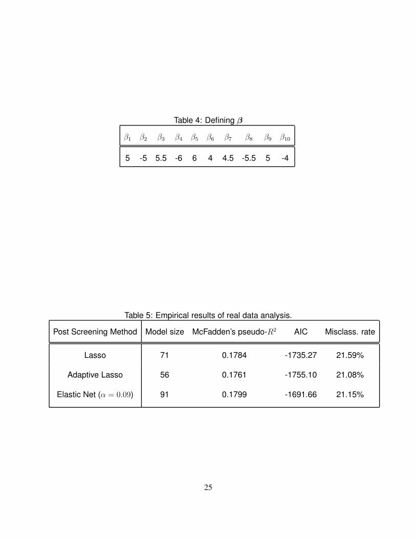
Table 4: Defining β

β1 β2 β3 β4 β5 β6 β7 β8 β9 β10

5 -5 5.5 -6 6 4 4.5 -5.5 5 -4

Table 5: Empirical results of real data analysis.

Post Screening Method Model size McFadden’s pseudo-R2 AIC Misclass. rate

Lasso 71 0.1784 -1735.27 21.59%

Adaptive Lasso 56 0.1761 -1755.10 21.08%

Elastic Net (α = 0.09) 91 0.1799 -1691.66 21.15%

25

5 Results of Simulations

Here we present the results of our four simulations. In each table of results, our newly proposed

method is referred to by the working title of CAT-SIS (Categorical-SIS).

Simulation 1 Results The results of Simulation 1 are summarized in Tables 6 through 10:




26

Table 6: Mean Minimum Model Sizes (n = 200, p = 5000)

CAT-SIS MMLE DC-SIS HLW-SIS

Mean Minimum Model Size 54.674 150.340 64.990 93.018

Table 7: Proportion of Replications Where Xj is in the Top d Causative Covariates

CAT-SIS

X1 X2 X3 X4 X5 X6 X7 X8 X9 X10

d = 10 0.864 0.980 0.988 0.832 1.000 0.998 0.844 0.974 0.836 0.858

d = 15 0.916 0.988 0.994 0.922 1.000 0.998 0.912 0.982 0.904 0.908

d = 20 0.920 0.988 0.994 0.930 1.000 0.998 0.926 0.990 0.930 0.930


MMLE

X1 X2 X3 X4 X5 X6 X7 X8 X9 X10

d = 10 0.210 0.680 0.690 0.250 0.786 0.816 0.194 0.646 0.182 0.218

d = 15 0.384 0.746 0.756 0.404 0.822 0.844 0.354 0.742 0.320 0.400

d = 20 0.508 0.796 0.800 0.490 0.854 0.864 0.452 0.796 0.440 0.490

27


DC-SIS

X1 X2 X3 X4 X5 X6 X7 X8 X9 X10

d = 10 0.850 0.978 0.982 0.818 0.998 0.998 0.804 0.968 0.824 0.834

d = 15 0.900 0.984 0.990 0.898 0.998 0.998 0.894 0.984 0.888 0.894

d = 20 0.916 0.988 0.992 0.920 0.998 0.998 0.922 0.986 0.908 0.914


HLW-SIS

X1 X2 X3 X4 X5 X6 X7 X8 X9 X10

d = 10 0.808 0.956 0.962 0.800 0.992 0.996 0.778 0.954 0.760 0.802

d = 15 0.862 0.974 0.980 0.864 0.994 0.998 0.860 0.966 0.854 0.862

d = 20 0.890 0.980 0.986 0.886 0.994 0.998 0.872 0.972 0.886 0.882


CAT-SIS MMLE DC-SIS HLW-SIS


28


CAT-SIS

X1 X2 X3 X4 X5 X6 X7 X8 X9 X10

d = 10 0.828 0.822 0.816 0.866 0.884 0.820 0.892 0.850 0.796 0.862

d = 15 0.876 0.876 0.882 0.904 0.924 0.874 0.920 0.906 0.878 0.900

d = 20 0.888 0.892 0.898 0.918 0.940 0.902 0.936 0.920 0.898 0.920


MMLE

X1 X2 X3 X4 X5 X6 X7 X8 X9 X10

d = 10 0.028 0.026 0.038 0.038 0.424 0.016 0.302 0.054 0.014 0.124

d = 15 0.072 0.060 0.066 0.078 0.554 0.054 0.388 0.098 0.032 0.204

d = 20 0.110 0.098 0.106 0.152 0.612 0.086 0.468 0.166 0.064 0.270


DC-SIS

X1 X2 X3 X4 X5 X6 X7 X8 X9 X10

d = 10 0.832 0.832 0.830 0.868 0.860 0.824 0.880 0.860 0.818 0.868

d = 15 0.876 0.884 0.886 0.904 0.886 0.880 0.880 0.910 0.878 0.906

d = 20 0.898 0.900 0.908 0.918 0.918 0.904 0.930 0.918 0.896 0.930

29


HLW-SIS

X1 X2 X3 X4 X5 X6 X7 X8 X9 X10

d = 10 0.754 0.766 0.744 0.774 0.846 0.752 0.844 0.776 0.738 0.808

d = 15 0.820 0.806 0.816 0.842 0.876 0.806 0.876 0.830 0.820 0.858

d = 20 0.844 0.830 0.850 0.862 0.880 0.824 0.888 0.862 0.838 0.876


CAT-SIS DC-SIS MMLE HLW-SIS



CAT-SIS

X1 X2 X3 X4 X5

d = 10 1.000 0.834 0.804 0.810 0.816

d = 15 1.000 0.860 0.858 0.842 0.862

d = 20 1.000 0.878 0.886 0.874 0.894

30


MMLE

X1 X2 X3 X4 X5

d = 10 1.000 0.822 0.798 0.808 0.824

d = 15 1.000 0.856 0.868 0.842 0.870

d = 20 1.000 0.882 0.892 0.872 0.890


DC-SIS

X1 X2 X3 X4 X5

d = 10 1.000 0.832 0.808 0.806 0.814

d = 15 1.000 0.860 0.850 0.838 0.866

d = 20 1.000 0.880 0.880 0.864 0.890


HLW-SIS

X1 X2 X3 X4 X5

d = 10 1.000 0.742 0.708 0.710 0.740

d = 15 1.000 0.794 0.758 0.778 0.790

d = 20 1.000 0.832 0.806 0.800 0.828

31


CAT-SIS DC-SIS

Mean Minimum Model Size 95.610 142.084


CAT-SIS

X1 X2 X3 X4 X5 X6 X7 X8 X9 X10

d = 10 0.874 0.498 0.804 0.746 0.998 1.000 0.928 0.702 0.580 0.534

d = 15 0.934 0.622 0.874 0.840 1.000 1.000 0.964 0.806 0.710 0.660

d = 20 0.954 0.678 0.910 0.894 1.000 1.000 0.978 0.868 0.762 0.728


DC-SIS

X1 X2 X3 X4 X5 X6 X7 X8 X9 X10

d = 10 0.832 0.444 0.762 0.678 0.992 1.000 0.914 0.648 0.534 0.468

d = 15 0.900 0.550 0.838 0.768 0.998 1.000 0.950 0.742 0.640 0.564

d = 20 0.926 0.620 0.874 0.828 1.000 1.000 0.964 0.796 0.712 0.650

32

6 Proofs of Theoretical Results

Here we present in full the proofs for Theorems 1 and 2 given at 3.0.1 and 3.0.2. Before proceeding

into the proofs, we will establish a pair of lemmas which employ the Mann-Wald Theorem [see

31].

Prefacing Lemmas These lemmas will lead into our proof of our main theorems on (strong) sure

screening.

6.0.1 A lemma

[See 35, Theorem of Section 1.7].

Let σj and σY be the estimators of σj and σY used in the definition of ˆj . Assume that σj ,

σY , and τj are all (individually speaking) consistent estimators of the respective values they are

estimating (viz. σj , σY , and cov(Xj, Y )). Then we have that in fact

ˆj =τj

σj σY

is a consistent estimator of j .

Proof. We will employ the Mann-Wald theorem (also known as the Continuous Mapping Theo-

rem) twice. This theorem asserts that Borel functions that are almost everywhere continuous on

Rk (or a Borel subset of such) preserve convergence in probability. This implies that if α is a con-

33

sistent estimator of A and ζ is a consistent estimator of Z, then for any Borel function f satisfying

the aforementioned conditions,

f(α, ζ)p−→ f(A,Z)

and thus f(α, ζ) is a consistent estimator of f(A,Z).

Define the function

f(a, b) =1

ab

on Rk>0 = (0,∞)k (All positive real-valued k-vectors). This function is continuous on its entire

domain. (Note that, in line with condition (C1), we can assume (WLOG) that σj and σY are both

positive). Hence f is a well defined and continuous function for operands a = σj and b = σY .

This implies by the Mann-Wald theorem that in fact 1σj σY

is a consistent estimator for 1σjσY

.

It is taken as a given that standard binary multiplication is a Borel function on Rk (since

multiplication is in fact continuous on all of Rk). We implicitly use this fact above to assume that

(σj σY )p−→ (σjσY ).

Furthermore, this assumption on standard multiplication implies, again by the Mann-Wald theo-

rem, that in fact

ˆj = τj1

σj σY=

τjσj σY

is a consistent estimator of j . (Note that this result is contingent upon knowing that τj is a

consistent estimator of cov(Xj, Y ). This is to be shown below). The desired result has been

achieved.

34

6.0.2 Lemma on Consistency of an Estimator of Standard Deviation

It is a classical result (reproduced in its entirety below) that for any realizations W1, W2, . . . , Wn

of a bounded random variable W ,

S2 =1

n

n∑

i=1

(Wi − W )2

is a consistent estimator of Var(W ), where W = 1n

∑Wi. As a simple corollary to this, we can

once again use the Mann-Wald Theorem to get that S is a consistent estimator of the standard

deviation of W .

Proof. Write the variance of W as σ2. It is a rudimentary result that

E(S2) =(n− 1)

nσ2 < σ2.

This means that S2 is in fact a biased estimator of σ2. Let σ2 denote the traditional (and unbiased)

estimator of σ2:

σ2 =1

n− 1

n∑

i=1

(Wi − W )2

It is clear that S2 = n−1nσ2. It follows that

Var(S2) = Var

(n− 1

nσ2

)=

(n− 1

n

)2

Var(σ2).

Furthermore, it can be established [see e.g. 7] that

Var(σ2) =1

n

(µ4 −

n− 3

n− 1µ22

),

35

where µℓ =1n

∑(Wi−EW )ℓ (with ℓ = 2 or ℓ = 4). Since W is taken as being bounded, we know

that |µℓ| < ∞.

Employing Chebychev’s inequality for any ε > 0, we get the following:

(P(|S2 − σ2| ≥ ε)

)∼ P(|σ2 − σ2| ≥ ε) ≤

Var(σ2)

ε2.

Ergo, if we can show that the variance of σ2 approaches 0 as n goes to ∞, it will follow

that S2 converges to σ2 in probability (and hence is a consistent estimator of σ2). However, we

established above that

Var(σ2) =1

n

(µ4 −

n− 3

n− 1µ22

),

which clearly approaches 0 as n goes to infinity. This confirms that in fact S2 is a consistent esti-

mator of σ2. Note in conclusion that this implies by the Mann-Wald theorem that S is a consistent

estimator of σ.

The lemma at 6.0.2 establishes that indeed σj and σY are consistent estimators of the respec-

tive standard deviations of Xj and Y .

We now proceed into the proofs of our main theorems on sure screening.

Proofs of Theorems 1 and 2 The proof of these two theorems is accomplished in three steps:

1. We show that a positive lower bound min exists for all j with j ∈ ST . That is, we show the

36

following:

There exists min > 0 such that j > min for all j ∈ ST .

2. We then show that ˆj is a uniformly consistent estimator of j for each 1 ≤ j ≤ p. This will

actually consist of showing that τj is a consistent estimator of cov(Xj, Y ), since the terms

in the denominator of ˆj are already well established consistent estimators of the standard

deviations of Xj and Y . (Refer to the lemma at 6.0.2).

3. We finally show that there exists said constant c > 0 such that

P(S = ST ) −→ 1 as n −→ ∞

(with weak consistency being shown as a natural subcase).

6.0.3 Step 1

We know that

ω(j)km =

∣∣∣(v(j)k − E(Xj))(m− E(Y ))p(j)km

∣∣∣

Hence, for j ∈ ST ,

j =

∑1≤k≤Kj

0≤m≤1

ω(j)km

σjσY≥

1

σ2max

∑

1≤k≤Kj

0≤m≤1

ω(j)km by (C1),

≥1

σ2max

max1≤k≤Kj

0≤m≤1

ω(j)km

37

≥ωmin

σ2max

by (C2),

> 0.

Define min =ωmin

2σ2max

. Then j > min > 0 for all j ∈ ST . This establishes a positive lower bound

on j for all j ∈ ST , completing Step 1. Corollary 1 at 3.0.3 is also established by this step.

6.0.4 Step 2

We now need to discuss two equal forms of the numerator τj of ˆj . It has been established that we

desire to use τj as an estimator of cov(Xj , Y ). We show that in fact τj is equal to the following

estimator for cov(Xj , Y ) :

1

n

n∑

i=1

(Xij − Xj)(Yi − Y ) ≈ cov(Xj , Y ), (1)

where Xj =1n

∑Xij and Y = 1

n

∑Yi as before.

Specific to our case currently, we know that Yi ∈ {0, 1}. Assume WLOG that Xij ∈

{v(j)1 , v

(j)2 , . . . , v

(j)Kj}. Then Xj = v(j). Let nkm denote the number of observations satisfying

Xij = k and Yi = m. It follows that p(j)km = nkm

n. We can rewrite (1) as follows:

(1) =1

n

∑

1≤i≤nYi=1

(Xij − Xj)(1− Y )−1

n

∑

1≤i≤nYi=0

(Xij − Xj)(Y )

38

=1

n

((v

(j)1 − v(j))(1− Y )n11 + · · ·+ (v

(j)Kj

− v(j))(1− Y )nKj1

)

−1

n

((v

(j)1 − v(j))(Y )n10 + · · ·+ (v

(j)Kj

− v(j))(Y )nKj0

)

=1

n

∑

1≤k≤Kj

0≤m≤1

(v(j)k − v(j))(m− Y )nkm

=∑

1≤k≤Kj

0≤m≤1

(v(j)k − v(j))(m− Y )p

(j)km

= τj .

So indeed (1) is equal to our previously given formula for τj . As convenient, we will use the form

(1) when discussing τj .

We now apply the weak law of large numbers to show that ˆj is a (uniformly) consistent

estimator of j . This will consist of showing that τj is a consistent estimator of cov(Xj , Y ), since

the denominator of ˆj is comprised of the routine (and, importantly here, consistent) estimators of

σj and σY . Since it can be show via a standard argument using the Mann-Wald Theorem that the

quotient of consistent estimators is itself a consistent estimator, our aforementioned work with τj

will suffice.

By expanding the product of binomials in (1), we get

τj =1

n

∑XijYi −

1

n

∑XjYi −

1

n

∑XijY +

1

n

∑XjY

︸︷︷︸→E(Xj)E(Y )

.

39

By several applications (summand wise) of the weak law of large numbers to this above

expression, we know:

1

n

∑XijYi

p−→ E(XjY )

1

n

∑XjYi

p−→ E(Xj)E(Y )

1

n

∑XijY

p−→ E(Xj)E(Y ),

with all convergence being in probability.

Hence we have

τj =1

n

∑XijYi −

1

n

∑XjYi −

1

n

∑XijY +

1

n

∑XjY

p−→ E(XjY )− 2E(Xj)E(Y ) + E(Xj)E(Y )

= E(XjY )− E(Xj)E(Y )

= cov(Xj , Y ).

So indeed τj is a consistent estimator of cov(Xj, Y ). This in turn shows, by the lemma at

6.0.1, that ˆj is consistent as an estimator of j .

It is a simple step to show that such consistency is uniform. This is done as follows: Since

ˆj is consistent as an estimator of j , we know that for any 1 ≤ j ≤ p and any ε > 0,

P(| ˆj − j | > ε) → 0 as n → ∞.

40

Let J = argmax1≤j≤p | ˆj − j |. Then, since J ∈ {1, 2, . . . , p} itself, we indeed know that

P(| ˆJ − J | > ε) → 0 as n → ∞

for any ε > 0. In other words, we have that

P

(max1≤j≤p

| ˆj − j | > ε

)→ 0 as n → ∞

for any ε > 0. This shows that ˆj is a uniformly consistent estimator of j , completing Step 2. We

also have established the claims of Corollary 2 found at 3.0.4.

6.0.5 Step 3

(This follows 24 closely).

In Step 1 we defined

min =ωmin

2σ2max

.

Let c = (2/3)min. Suppose by way of contradiction that this c is insufficient to be able to claim

S ⊇ ST . This would mean that there exists some j∗ ∈ ST , yet j∗ /∈ S . It then follows that we must

have

ˆj∗ ≤ (2/3)min

while at the same time having (as shown in Step 1)

j∗ > min.

41

From this we can conclude that | ˆj∗ − j∗| > (1/3)min, which implies that max1≤j≤p | ˆj −

j | > (1/3)min as well.

However, we know by the uniform consistency of ˆj that by letting ε = 1/3min, we have

P(S 6⊇ ST ) ≤ P

(max1≤j≤p

| ˆj − j | > (1/3)min

)→ 0 as n → ∞.

This is a contradiction to the assumption of non containment above. So indeed, we have that

P(S ⊇ ST ) → 1 as n → ∞.

This proves Theorem 2, and is the forward direction for proving Theorem 1.

To prove the reverse direction for Theorem 1, suppose (again by way of contradiction) that

S 6⊆ ST . Then there is some j∗ ∈ S , yet j∗ /∈ ST . This means that

ˆj∗ ≥ (2/3)min,

while at the same time (by (C2)) having

j∗ = 0.

It now follows that

| ˆj∗ − j∗| > (2/3)min.

Set ε = (2/3)min. By uniform consistency we have

P(ST 6⊇ S) ≤ P

(max1≤j≤p

| ˆj − j | > (2/3)min

)→ 0 as n → ∞.

42

From this we know that

P(ST ⊇ S) → 1 as n → ∞.

In all, we can conclude that for c = (2/3)min, we have P(ST = S) → 1 as n → ∞,

completing the proof.

1. Alan Agresti. An Introduction to Categorical Data Analysis. Wiley, Hoboken, NJ, 2 edition,

2007.

2. A. Antoniadis and J. Fan. Regularization of wavelets approximations. Journal of the American

Statistical Association, 96:939–967, 2001.

3. P. Armitage. Tests for linear trends in proportions and frequencies. Biometrics, 11(3):375–386,

1955.

4. Krishnakumar Balasubramanian, Bharath K. Sriperumbudur, and Guy Lebanon. Ultrahigh

dimensional feature screening via rkhs embeddings. In Proceedings of the 16th International

Conference on Artificial Intelligence and Statistics (AISTATS), volume 31, pages 126–134,

Scottsdale, AZ, USA., 2013.

5. Leo Breiman. Random forests. Machine learning, 45(1):5–32, 2001.

6. E. Candes and T Tao. The dantzig selector: statistical estimation when p is much larger than

n (with discussion). The Annals of Statistics, 35(6):2313–2404, 2007.

43

7. E.C. Cho and M.J. Cho. Variance of sample variance. In JSM Proceedings: Survey Research

Methods Section, pages 1291–1293, Alexandria, VA, 2008. American Statistical Association.

8. William G. Cochran. Some methods for strengthening the common ÏG<sup>2</sup> tests.

Biometrics, 10(4):417–451, 1954.

9. Hengjian Cui, Runze Li, and Wei Zhong. Model-free feature screening for ultrahigh dimen-

sional discriminant analysis. Journal of the American Statistical Association, 110(510):630–

641, 2015.

10. T. Domencich and D. McFadden. Urban travel demand: A behavioral analysis. In D.W. Jor-

genson and J Waelbroeck, editors, Contributions to Economic Analysis. North-Holland Pub-

lishing Co, Amsterdam, 1975.

11. D.L. Donoho. High-dimensional data: The curse and blessings of dimensionality, 2000. Los

Angeles: Amer Math Soc Conference Math Challenges of 21st Century.

12. Bradley Efron, Trevor Hastie, Iain Johnstone, and Robert Tibshirani. Least angle regression.

The Annals of Statistics, 32(2):407–499, 04 2004.

13. J. Fan and Y. Fan. High-dimensional classification using features annealed independence rules.

The Annals of Statistics, 36(6):2605–2637, 2008.

14. J. Fan, Y. Feng, and R. Song. Nonparametric independence screening in sparse ultra-high

dimensional additive models. Journal of American Statistical Association, 106(494):544–557,

2011.

44

15. J. Fan, F. Han, and H. Liu. Challenges of big data analysis. National Science Review, (1):293–

314, 2014.

16. J. Fan and R Li. Statistical challenges with high dimensionality: feature selection in knowl-

edge discovery. In M. Sanz-Sole, J. Soria, J.L. Varona, and J. Verdera, editors, Proceedings

of the International Congress of Mathematicians, volume III, pages 595–622, Zurich, 2006.

European Mathematical Society.

17. J. Fan and J. Lv. Sure independence screening for ultrahigh dimensional feature space. Journal

of the Royal Statistical Society, Series B, 70(5):849–911, 2008.

18. J. Fan, R. Samworth, and Y. Wu. Ultrahigh dimensional variable selection: beyond the linear

model. Journal of Machine Learning Research, 10(3):1829–1853, 2009.

19. J. Fan and R. Song. Sure independence screening in generalized linear models with np-

dimensionality. Annals of Statistics, 38(6):3567–3604, 2010.

20. I. E. Frank and J. H. Friedman. A statistical view of some chemometrics regression tools (with

discussion). Technometrics, 35:109–148, 1993.

21. Jerome Friedman, Trevor Hastie, and Robert Tibshirani. Regularization paths for generalized

linear models via coordinate descent. Journal of Statistical Software, 33(1):1–22, 2010.

22. Guoyu Guan, Jianhua Guo, and Hansheng Wang. Varying naïve bayes models with applica-

tions to classification of chinese text documents. Journal of Business and Economic Statistics,

32(3):445–456, 2014.

45

23. Trevor Hastie, Robert Tibshirani, and Jerome Friedman. The Elements of Statistical Learning.

Springer, New York, 2 edition, 2009.

24. Danyang Huang, Runze Li, and Hansheng Wang. Feature screening for ultrahigh dimensional

categorical data with applications. Journal of Business and Economic Statistics, 32(2):237–

244, 2014.

25. Hyunsoo Kim, Peg Howland, and Haesun Park. Dimension reduction in text classification

with support vector machines. Journal of Machine Learning Research, 6(Jan):37–53, 2005.

26. Jing Kong, Sijian Wang, and Grace Wahba. Using distance covariance for improved variable

selection with application to learning genetic risk models. Statistics in Medicine, 34(10):1708–

1720, 2015.

27. R Li, W Zhong, and L Zhu. Feature screening via distance correlation learning. Journal of the

American Statistical Association, 107(499):1129–1139, 2012.

28. Andy Liaw and Matthew Wiener. Classification and regression by randomforest. R News,

2(3):18–22, 2002.

29. J Liu, R Li, and R Wu. Feature selection for varying coeffcient models with ultrahigh dimen-

sional covariates. Journal of the American Statistical Association, 109(505):266–274, 2014.

30. J.J. Louviere, D.A. Hensher, and J.D. Swait. Stated Choice Methods: Analysis and Applica-

tions. Cambridge University Press, 2000.

46

31. H. B. Mann and A. Wald. On stochastic limit and order relationships. The Annals of Mathe-

matical Statistics, 14(3):217–226, 1943.

32. D. McFadden. Conditional logit analysis of qualitative choice behavior. In P. Zarembka, editor,

Frontiers in Econometrics, chapter 4, pages 105–142. Academic Press, New York, 1974.

33. Scott Menard. Coeffcients of determination for multiple logistic regression analysis. The

American Statistician, 504(1):17–24, 2000.

34. T Popoviciu. Sur les Ãl’quations algÃl’briques ayant toutes leurs racines rÃl’elles. Mathemat-

ica (Cluj), 9:129–145, 1935.

35. R. J. Serfling. Approximation Theorems of Mathematical Statistics. Wiley, New York, 1980.

36. GÃabor J. Székely and Maria L. Rizzo. Brownian distance covariance. Ann. Appl. Stat.,

3(4):1236–1265, 12 2009.

37. GÃabor J. Székely, Maria L. Rizzo, and Nail K. Bakirov. Measuring and testing dependence

by correlation of distances. Ann. Statist., 35(6):2769–2794, 12 2007.

38. R. Tibshirani. Regression shrinkage and selection via lasso. Journal of the Royal Statistical

Society: Series B, 58:267–288, 1996.

39. Simon Tong and Daphne Koller. Support vector machine active learning with applications to

text classification. Journal of machine learning research, 2(Nov):45–66, 2001.

40. Chen Xu and Jiahua Chen. The sparse mle for ultrahigh-dimensional feature screening. Jour-

nal of the American Statistical Association, 109(507):1257–1269, 2014.

47

41. W Zhong and L Zhu. An iterative approach to distance correlation-based sure independent

screening. Journal of Statistical Computation and Simulation, pages 1–15, 2014.

42. Li-Ping Zhu, Lexin Li, Runze Li, and Li-Xing Zhu. Model-free feature screening for ultra-

high dimensional data. Journal of the American Statistical Association, 106(496):1464–1475,

2011.

43. Hui Zou. The adaptive lasso and its oracle properties. Journal of the American Statistical

Association, 101(476):1418–1429, 2006.

44. Hui Zou and Trevor Hastie. Regularization and variable selection via the elastic net. Journal

of the Royal Statistical Society, Series B, 67(2):301–320, 2005.

48

strong sure screening of ultra-high dimensional cate ... · strong sure screening of ultra-high...

Documents