STRINGdb Package Vignette

Andrea Franceschini

15 March 2015

1 INTRODUCTION

STRING (http://www.string-db.org) is a database of known and predicted protein-protein interac-tions. The interactions include direct (physical) and indirect (functional) associations. The databasecontains information from numerous sources, including experimental repositories, computational pre-diction methods and public text collections. Each interaction is associated with a combined confidencescore that integrates the various evidences. We currently cover 5’214’234 proteins from 1133 organisms.

As you will learn in this guide, the STRING database can be usefull to add meaning to list of genes(e.g. the best hits coming out from a screen or the most differentially expressed genes coming out froma Microarray/RNAseq experiment.)

We provide the STRINGdb R package in order to facilitate our users in accessing the STRINGdatabase from R. In this guide we explain, with examples, most of the package’s features and function-alities.

In the STRINGdb R package we use the new ReferenceClasses of R (search for ”ReferenceClasses”in the R documentation.). Besides we make use of the iGraph package (http://igraph.sourceforge.net)as a data structure to represent our protein-protein interaction network.

To begin, you should first know the NCBI taxonomy identifiers of the organism on which you haveperformed the experiment (e.g. 9606 for Human, 10090 for mouse). If you don’t know that, you cansearch the NCBI Taxonomy (http://www.ncbi.nlm.nih.gov/taxonomy) or start looking at our speciestable (that you can also use to verify that your organism is represented in the STRING database).Hence, if your species is not Human (i.e. our default species), you can use this function to retrieve/searchour species table:

> get_STRING_species(version="10", species_name=NULL)

> library(STRINGdb)

> string_db <- STRINGdb$new( version="10", species=9606,

+ score_threshold=0, input_directory="" )

As it has been shown in the above commands, you start instantiating the STRINGdb reference class.In the constructor of the class you can also define the STRING version to be used and a threshold forthe combined scores of the interactions, such that any interaction below that threshold is not loaded inthe object (by default the score threshold is set to 400 ! ).

1

Besides, if you specify a local directory to the parameter input-directory, all the database files will bedownloaded into this directory and the package can then be used off-line. Otherwise, the database fileswill be saved and cached in a temporary directory that will be cleaned automatically when the R sessionis closed.

For a better understanding of the package two other commands can be useful:

> STRINGdb$methods() # To list all the methods available.

[1] "add_diff_exp_color" "add_proteins_description"

[3] "benchmark_ppi" "benchmark_ppi_pathway_view"

[5] "callSuper" "copy"

[7] "enrichment_heatmap" "export"

[9] "field" "getClass"

[11] "getRefClass" "get_aliases"

[13] "get_annotations" "get_annotations_desc"

[15] "get_bioc_graph" "get_clusters"

[17] "get_enrichment" "get_graph"

[19] "get_homologs" "get_homologs_besthits"

[21] "get_homology_graph" "get_interactions"

[23] "get_link" "get_neighbors"

[25] "get_pathways_benchmarking_blackList" "get_png"

[27] "get_ppi_enrichment" "get_ppi_enrichment_full"

[29] "get_proteins" "get_pubmed"

[31] "get_pubmed_interaction" "get_subnetwork"

[33] "get_summary" "get_term_proteins"

[35] "import" "initFields"

[37] "initialize" "load"

[39] "load_all" "map"

[41] "mp" "plot_network"

[43] "plot_ppi_enrichment" "post_payload"

[45] "remove_homologous_interactions" "set_background"

[47] "show" "show#envRefClass"

[49] "trace" "untrace"

[51] "usingMethods"

> STRINGdb$help("get_graph") # To visualize their documentation.

Call:

$get_graph()

Description:

Return an igraph object with the entire STRING network.

We invite the user to use the functions of the iGraph package to conveniently

search/analyze the network.

References:

Csardi G, Nepusz T: The igraph software package for complex network research,

2

InterJournal, Complex Systems 1695. 2006.

http://igraph.sf.net

See Also:

In order to simplify the most common tasks, we do also provide convenient functions

that wrap some iGraph functions.

get_interactions(string_ids) # returns the interactions in between the input proteins

get_neighbors(string_ids) # Get the neighborhoods of a protein (or of a vector of proteins).

get_subnetwork(string_ids) # returns a subgraph from the given input proteins

Author(s):

Andrea Franceschini

For all the methods that we are going to explain below, you can always use the help function inorder to get additional information/parameters with respect to those explained in this guide.

As an example, we use the analyzed data of a microarray study taken from GEO (Gene ExpressionOmnibus, GSE9008). This study investigates the activity of Resveratrol, a natural phytoestrogen foundin red wine and a variety of plants, in A549 lung cancer cells. Microarray gene expression profiling after48 hours exposure to Revestarol has been performed and compared to a control composed by A549lung cancer cells threated only with ethanol. This data is already analyzed for differential expressionusing the limma package: the genes are sorted by fdr corrected pvalues and the log fold change of thedifferential expression is also reported in the table.

> data(diff_exp_example1)

> head(diff_exp_example1)

pvalue logFC gene

1 0.0001018 3.333461 VSTM2L

2 0.0001392 3.822383 TBC1D2

3 0.0001720 3.306056 LENG9

4 0.0001739 3.024605 TMEM27

5 0.0001990 3.854414 LOC100506014

6 0.0002393 3.082052 TSPAN1

As a first step, we map the gene names to the STRING database identifiers using the ”map” method.In this particular example, we map from gene HUGO names, but our mapping function supports severalother common identifiers (e.g. Entrez GeneID, ENSEMBL proteins, RefSeq transcripts ... etc.).

The map function adds an additional column with STRING identifiers to the dataframe that is passedas first parameter.

> example1_mapped <- string_db$map( diff_exp_example1, "gene", removeUnmappedRows = TRUE )

Warning: we couldn't map to STRING 14% of your identifiers

3

As you may have noticed, the previous command prints a warning showing the number of genesthat we failed to map. In this particular example, we cannot map all the probes of the microarray thatrefer to position of the chromosome that are not assigned to a real gene (i.e. all the LOC genes). If weremove all these LOC genes before the mapping we obtain a much lower percentage of unmapped genes(i.e. < 6 %).If you set to FALSE the ”removeUnmappedRows” parameter, than the rows which corresponds tounmapped genes are left and you can manually inspect them.Finally, we extract the best 200 genes and we produce an image of the STRING network for those. Theimage shows clearly the genes and how they are possibly functionally related. On the top of the plot, weinsert a pvalue that represents the probability that you can expect such an equal or greater number ofinteractions by chance. Besides, on the bottom, there is a short-url that points to the relative page onour web-interface. You can copy and paste that url on your favorite browser and/or send it via e-mailto your colleagues or insert it in publications.

> hits <- example1_mapped$STRING_id[1:200]

> string_db$plot_network( hits )

4

proteins: 200interactions: 353

expected interactions: 266 (p−value: 2.60548724706489e−07)

http://string−db.org/10/p/53659871

5

2 PAYLOAD MECHANISM

This R library provides the ability to interact with the STRING payload mechanism. The payloadappears as an additional colored ”halo” that starts from the boder of the bubbles.

For example, this allows to color in green the genes that are down-regulated and in red the genesthat are up-regulated. For this mechanism to work, we provide a function that posts the informationon our web server.

> # filter by p-value and add a color column

> # (i.e. green down-regulated gened and red for up-regulated genes)

> example1_mapped_pval05 <- string_db$add_diff_exp_color( subset(example1_mapped, pvalue<0.05),

+ logFcColStr="logFC" )

> # post payload information to the STRING server

> payload_id <- string_db$post_payload( example1_mapped_pval05$STRING_id,

+ colors=example1_mapped_pval05$color )

> # display a STRING network png with the "halo"

> string_db$plot_network( hits, payload_id=payload_id )

6

proteins: 200interactions: 353

expected interactions: 266 (p−value: 2.60548724706489e−07)

http://string−db.org/10/p/28529872

7

3 ENRICHMENT

We provide a method to compute (and visualize) the enrichment in protein-protein interactions along asorted list of proteins. In the context of genome-wide screens (e.g. RNAi or proteomics), it can be usefulto visualize the distribution of the enrichment in the resulting sorted list of genes. If the experimentwas successful, and the top hits have protein-protein interactions, you should see more enrichment atthe beginning of the list than at the end. Besides, you can also use the enrichment graph to help youto define a threshold on the number of proteins to consider (for example, if you see a strong enrichmentup to position 600 on your list, this means that the signal is probably sparsed to cover the best 600genes).

> # plot the enrichment for the best 1000 genes

> string_db$plot_ppi_enrichment( example1_mapped$STRING_id[1:1000], quiet=TRUE )

● ●●

●

●

●

●

●●

●●

● ●

● ● ● ●

●

●

●

● ●

●

●

●

●

●

●

●

●

●

●

●

●

●● ●

●

●

●

● ●

●

●

●

●

●

●

●●

0 200 400 600 800 1000

−10

−8

−6

−4

−2

0

PPI Enrichment

8

We also provide a method to compute the enrichment in Gene Ontology, KEGG pathway andInterpro domains, similar to the ”enrichment” widget in our web-interface. The enrichment is computedusing an hypergeometric test. The multiple testing correction method can be changed (setting themethodMT parameter) and it is also possible to specify whether to use the ”Inferred from ElettronicAnnotations” or only the manually curated annotations.

> enrichmentGO <- string_db$get_enrichment( hits, category = "Process", methodMT = "fdr", iea = TRUE )

> enrichmentKEGG <- string_db$get_enrichment( hits, category = "KEGG", methodMT = "fdr", iea = TRUE )

> head(enrichmentGO, n=7)

term_id proteins hits pvalue pvalue_fdr

1 GO:0010466 197 10 3.552195e-06 0.003477795

2 GO:0043207 596 17 4.532314e-06 0.003477795

3 GO:0051707 596 17 4.532314e-06 0.003477795

4 GO:0009607 624 17 8.283470e-06 0.004767137

5 GO:0002252 399 13 1.602950e-05 0.006175628

6 GO:0010951 188 9 1.765641e-05 0.006175628

7 GO:0033993 670 17 2.069460e-05 0.006175628

term_description

1 negative regulation of peptidase activity

2 response to external biotic stimulus

3 response to other organism

4 response to biotic stimulus

5 immune effector process

6 negative regulation of endopeptidase activity

7 response to lipid

> head(enrichmentKEGG, n=7)

term_id proteins hits pvalue pvalue_fdr

1 04115 66 6 9.969204e-08 1.475442e-05

2 04610 68 5 3.577966e-06 2.647695e-04

3 05168 174 5 3.254067e-04 1.605340e-02

4 01100 1161 12 5.277721e-04 1.952757e-02

5 04380 123 4 8.399948e-04 2.486385e-02

6 00590 61 3 1.197959e-03 2.638087e-02

7 05161 139 4 1.322517e-03 2.638087e-02

term_description

1 p53 signaling pathway

2 Complement and coagulation cascades

3 Herpes simplex infection

4 Metabolic pathways

5 Osteoclast differentiation

6 Arachidonic acid metabolism

7 Hepatitis B

If you have performed your experiment on a predefined set of proteins, it is important to run theenrichment statistics using that set as a background (otherwise you would get a wrong p-value !). Hence,before to launch the methods explained above, you should set the background:

9

> backgroundV <- example1_mapped$STRING_id[1:2000] # as an example, we use the first 2000 genes

> string_db$set_background(backgroundV)

You can also set the background when you instantiate the STRINGdb object:

> string_db <- STRINGdb$new( score_threshold=0, backgroundV = backgroundV )

If you want to compare the enrichment of two or more lists of genes (e.g. the results of two experiments),you can use our HEATMAP visualization option:

> eh <- string_db$enrichment_heatmap( list( hits[1:100], hits[101:200]),

+ list("list1","list2"), title="My Lists" )

list1

list2

leukocyte mediated immunity

zymogen activation

negative regulation of catalytic activity

intrinsic apoptotic signaling pathway in response to DNA damage by p53 class mediator

establishment of planar polarity involved in neural tube closure

negative regulation of hydrolase activity

negative regulation of endopeptidase activity

positive regulation of protein activation cascade

positive regulation of complement activation

positive regulation of activation of membrane attack complex

response to biotic stimulus

regulation of endopeptidase activity

intrinsic apoptotic signaling pathway in response to DNA damage

response to other organism

response to external biotic stimulus

regulation of proteolysis

immune effector process

defense response

negative regulation of peptidase activity

regulation of peptidase activity

regulation of protein processing

4.8 5 5.2Value

Color Key

10

4 CLUSTERING

The iGraph package provides several clustering/community algorithms: ”fastgreedy”, ”walktrap”, ”sp-inglass”, ”edge.betweenness”. We encapsulate this in an easy-to-use function that returns the clustersin a list.

> # get clusters

> clustersList <- string_db$get_clusters(example1_mapped$STRING_id[1:600])

> # plot first 4 clusters

> par(mfrow=c(2,2))

> for(i in seq(1:4)){

+ string_db$plot_network(clustersList[[i]])

+ }

11

proteins: 61interactions: 91

expected interactions: 7 (p−value: 0)

http://string−db.org/10/p/10359875

proteins: 120interactions: 881

expected interactions: 457 (p−value: 0)

http://string−db.org/10/p/79229876

proteins: 109interactions: 356

expected interactions: 82 (p−value: 0)

http://string−db.org/10/p/94439878

proteins: 166interactions: 1250

expected interactions: 407 (p−value: 0)

http://string−db.org/10/p/15249881

12

5 ADDITIONAL PROTEIN INFORMATION

You can get a table that contains all the proteins that are present in our database. The protein tablealso include the name, the size and a short description of the proteins.

> string_proteins <- string_db$get_proteins()

In the following section we will show how to query STRING with R on some specific proteins. Inthe examples, we will use the famous tumor proteins TP53 and ATM .

First we need to get the STRING identifier of those proteins, using our mp method:

> tp53 = string_db$mp( "tp53" )

> atm = string_db$mp( "atm" )

The mp method (i.e. map proteins) is an alternative to our map method, to be used when you needto map only one or few proteins.It takes in input a vector of protein aliases and returns a vector with the STRING identifiers of thoseproteins.

Using the following method, you can see the proteins that interact with one or more of your proteins:

> string_db$get_neighbors( c(tp53, atm) )

It is also possible to retrieve the interactions that connect certain input proteins between each other.Using the ”get interactions” method we can clearly see that TP53 and ATM interact with each otherwith a good evidence/score.

> string_db$get_interactions( c(tp53, atm) )

from to neighborhood

1 9606.ENSP00000269305 9606.ENSP00000278616 258

neighborhood_transferred fusion cooccurence homology coexpression

1 165 2 527 891 160

coexpression_transferred experiments experiments_transferred database

1 78 999 960 900

database_transferred textmining textmining_transferred combined_score

1 312 973 80 999

Using the get pubmed interactions method we can retrieve the pubmed identifiers of the articlesthat contain the name of both the proteins (if any). Such articles could support to the interaction.

> string_db$get_pubmed_interaction( tp53, atm )

13

STRING also provides a way to get homologous proteins: in our database we store an ALL-AGAINST-ALL blast alignment of all our 5 million proteins. The method ”get homologs besthits”can be used to get the best hits of your proteins in all the >1000 STRING species (with the ”symbets”parameter you can limit the search to the reciprocal best hits. This increase the confidence to getorthologs and not paralogous proteins)

> # get the reciprocal best hits of the following protein in all the STRING species

> string_db$get_homologs_besthits(tp53, symbets = TRUE)

In addition, you can get all the homologous in a given species (i.e. all the blast hits):

> # get the homologs of the following two proteins in the mouse (i.e. species_id=10090)

> string_db$get_homologs(c(tp53, atm), target_species_id=10090, bitscore_threshold=60 )

6 BENCHMARKING PROTEIN-PROTEIN INTERACTIONS

When a new methodology/algorithm to infer protein-protein interactions is developed, the outcomeshould be carefully benchmarked against a gold standard. Hence, we suggest to benchmark agains theKEGG pathway database (or other high quality pathway databases), and we provide suitable functionsto perform this task.

First of all, you need to provide as input a sorted interaction data frame (with the columns ”pro-teinA”, ”proteinB”, ”score”).

> data(interactions_example)

> interactions_benchmark = string_db$benchmark_ppi(interactions_example, pathwayType = "KEGG",

+ max_homology_bitscore = 60, precision_window = 400, exclude_pathways = "blacklist")

Discarded 55844 interactions ( 79.77714 % ) between homologous proteins

NOTE: 717 interactions ( 5.1 % ) have been mapped to KEGG

The function benchmark ppi will return a data frame containing the sorted list of protein interactionsmapped to the benchmark, and the precision computed in a sliding window of 400 interactions (thatautomatically expands/shrink at the beginning/end of the sorted interactions list). The precision isdefined as the number of TP interactions (where the pair of proteins are both present together in atleast one pathway) vs the total number of interactions in the window. When benchmarking PPI it isoften important to remove the interactions composed by a pair of homologous protein. You can set aparameter in the function to automatically perform this task (max homology bitscore). The user mayalso want to remove several uninformative pathway from the gold standard (i.e. pathways that are toobig or too generic ). The STRING team manually curates a black list of KEGG pathways that in ouropinion should be removed in order to provide a reliable gold standard. With the ”exclude pathways”parameter it is possible to automatically remove those pathways from the analysis (setting the parameterto ”blacklist”) or to specify a vector contaning the term identifiers of the pathways that the user wantsto remove.

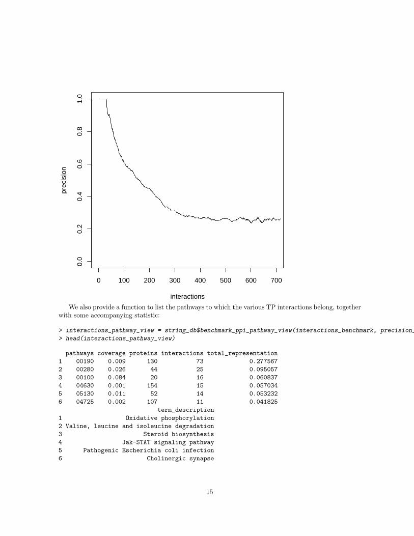
It is finally very easy to plot the precision vs the number of sorted interactions:

> plot(interactions_benchmark$precision, ylim=c(0,1), type="l", xlim=c(0,700),

+ xlab="interactions", ylab="precision")

14

0 100 200 300 400 500 600 700

0.0

0.2

0.4

0.6

0.8

1.0

interactions

prec

isio

n

We also provide a function to list the pathways to which the various TP interactions belong, togetherwith some accompanying statistic:

> interactions_pathway_view = string_db$benchmark_ppi_pathway_view(interactions_benchmark, precision_threshold=0.2, pathwayType = "KEGG")

> head(interactions_pathway_view)

pathways coverage proteins interactions total_representation

1 00190 0.009 130 73 0.277567

2 00280 0.026 44 25 0.095057

3 00100 0.084 20 16 0.060837

4 04630 0.001 154 15 0.057034

5 05130 0.011 52 14 0.053232

6 04725 0.002 107 11 0.041825

term_description

1 Oxidative phosphorylation

2 Valine, leucine and isoleucine degradation

3 Steroid biosynthesis

4 Jak-STAT signaling pathway

5 Pathogenic Escherichia coli infection

6 Cholinergic synapse

15

For each pathway for which a TP interaction is found in the sorted interaction list, we report its”total representation” (i.e. which percentages of interactions belong to that pathway), the ”coverage”(i.e. number of interactions of the input list in the pathway / total number of possible interactions inthe pathway) and the size of the pathway in number of proteins.

7 CITATION

Please cite:

Franceschini, A et al. (2013). STRING v9.1: protein-protein interaction networks, with increasedcoverage and integration. In:’Nucleic Acids Res. 2013 Jan;41(Database issue):D808-15. doi: 10.1093/nar/gks1094.Epub 2012 Nov 29

16